A05420112

IOSR Journal of Engineering (IOSRJEN) www.iosrjen.org

ISSN (e): 2250-3021, ISSN (p): 2278-8719

Vol. 05, Issue 04 (April. 2015), ||V2|| PP 01-12

International organization of Scientific Research 1 | P a g e

BMAP/BMSP/1 Queue with Randomly Varying Environment

Sandhya.R1, Sundar.V

2, Rama.G

3, Ramshankar.R

4, Ramanarayanan.R

5

1Independent Researcher MSPM, School of Business, George Washington University, Washington .D.C, USA

2Senior Testing Engineer, ANSYS Inc., 2600, Drive, Canonsburg, PA 15317,USA

3Independent Researcher B. Tech, Vellore Institute of Technology, Vellore, India

4Independent Researcher MS9EC0, University of Massachusetts, Amherst, MA, USA

5Professor of Mathematics, (Retired), Vel Tech University, Chennai, INDIA.

Abstract: This paper studies two stochastic batch Markovian arrival and batch Markovian service single server

queue BMAP/BMSP/1 queue Models (A) and (B) with randomly varying k* distinct environments. The arrival

process of the queue has matrix representation {Dmi : 0 ≤ m ≤ M} of order ki describing the BMAP and the

service process has matrix representation {Sni : 0 ≤ n ≤ N} of order k′i describing the BMSP respectively in the

environment i for 1 ≤ i ≤ k*. Whenever the environment changes from i to j the arrival BMAP and service

BMSP change from the i version to the j version with the exception of the first remaining arrival time and first

remaining service time in the new environment start as per stationary probability vector of j version of the

BMAP and of j version of the BMSP respectively for 1 ≤ i, j ≤ k*. The queue system has infinite storing

capacity and the state space is identified as five dimensional one to apply Neuts’ matrix methods. In the

environment i, the sizes of the arrivals and services are governed by the matrices Dmi and Sn

i , with respect to

environment. The service process is stopped when the queue becomes empty and is started with initial

probability vector of corresponding environment BMSP when the arrival occurs. Matrix partitioning method is

used to study the models. In Model (A) the maximum of the arrival sizes is greater than the maximum of the

service sizes and the infinitesimal generator is partitioned mostly as blocks of the sum of the products of BMAP

arrival and BMSP service phases in the various environments times the maximum of the arrival sizes for

analysis. In Model (B) the maximum of the arrival sizes is less than the maximum of the service sizes. The

generator is partitioned mostly using blocks of the same sum-product of batch Markovian phases times the

maximum of the service sizes. Block circulant matrix structure is noticed in the basic system generators. The

stationary queue length probabilities, its expected values, its variances and probabilities of empty levels are

derived for the two models using matrix methods. Numerical examples are presented for illustration.

Keywords: Batch Arrivals, Batch Services, Block Circulant Matrix, Neuts Matrix Methods, Phase Type

Distribution.

I. INTRODUCTION In this paper two batch arrival and batch service BMAP/BMSP/1 queues with random environment

have been studied using matrix geometric methods. Numerical studies on matrix methods are presented by Bini,

Latouche and Meini [1]. Multi server model has been of interest in Chakravarthy and Neuts [2]. Birth and death

model has been analyzed by Gaver, Jacobs and Latouche [3]. Analytic methods are focused in Latouche and

Ramaswami [4] and for matrix geometric methods one may refer Neuts [5]. For M/M/1 bulk queues with

random environment models one may refer Rama Ganesan, Ramshankar and Ramanarayanan [6] and M/M/C

bulk queues with random environment models are of interest in Sandhya, Sundar, Rama, Ramshankar and

Ramanarayanan [7]. PH/PH/1 bulk queues without variation of environments have been treated by Ramshankar,

Rama Ganesan and Ramanarayanan [8] and with variations of environment have been analyzed by

Ramshankar,Rama, Sandhya, Sundar and Ramanarayanan [9]. BMAP/M/C queue with bulk service and random

environment has been studied by Rama, Ramshankar, Sandhya, Sundar and Ramanarayanan [10]. The models

considered here are general compared to existing models. Batch Markovian service process (BMSP) considered

in this paper is similar to batch Markovian arrival process (BMAP) and BMAP has been studied by

Lucantony[11] and has been analyzed further by Cordeiro and Kharoufch [12] . When the queue becomes empty

the service process is stopped and it is started with starting probability vector when the arrivals occur in the

empty queue. Usually bulk arrival models have M/G/1 upper-Heisenberg block matrix structure. The

decomposition of a Toeplitz sub matrix of the infinitesimal generator is required to find the stationary

probability vector and matrix geometric structures are rarely noted. In such analysis the recurrence relation

method to find the stationary probabilities is stopped at a certain level in most general cases using a terminating

method very well explained by Qi-Ming He [13] and this stopping limitation of terminating method converts an

infinite arrival system to a finite arrival one. In special cases generating function has been identified by Rama



and Ramanarayanan [14]. However the method of partitioning of the infinitesimal generator along with

environment, BMAP phases and BMSP phases used in this paper is presenting matrix geometric solution for

finite sized batch arrivals and batch services models. The M/PH/1 and PH/M/C queues with random

environments have been studied by Usha [15] and [16] without bulk arrivals and bulk services. It has been

noticed by Usha [15, 16] that when the environment changes the remaining arrival and service times are to be

completed in the new environment. The residual arrival time and the residual service time distributions in the

new environment are to be considered in the new environment at an arbitrary epoch since the spent arrival time

and the spent service time have been in the previous environment with distinct sizes of PH phase. Further new

arrival time and new service time from the start using initial PH distributions of the new environment cannot be

considered since the arrival and the service have been partly completed in the previous environment indicating

the stationary versions of the arrival and service distributions in the new environments are to be used for the

completions of the residual arrival and service times in the new environment and on completion of the same the

next arrival and service onwards they have initial versions of the PH distributions of the new environment. The

stationary version of the distribution for residual time has been well explained in Qi-Ming He [13] where it is

named as equilibrium PH distribution. Randomly varying environment BMAP/BMSP/1 queue models have not

been treated so far at any depth.

Two models (A) and (B) on BMAP/BMSP/1 bulk queue systems with infinite storage space for

customers are studied here using the block partitioning method. Model (A) presents the case when M, the

maximum of the arrival sizes of BMAP is bigger than N, the maximum of the service sizes of BMSP. In Model

(B), its dual case N is bigger than M, is treated. In general in Queue models, the state space of the system has the

first co-ordinate indicating the number of customers in the system but here the customers in the system are

grouped and considered as members of blocks of sizes of the maximum for finding the rate matrix. Using the

maximum of the batch arrival sizes and of the batch service sizes and grouping the customers as members of

blocks in addition to coordinates of the arrival and service phases for partitioning the infinitesimal generator is a

new approach in this area. The matrices appearing as the basic system generators in these two models due to

block partitioned structure are seen as block circulant matrices. The paper is organized in the following manner.

In sections II and III the stationary probability of the number of customers waiting for service, the expectation

and the variance and the probability of empty queue are derived for these Models (A) and (B). In section IV

numerical cases are presented to illustrate them.

II. MODEL (A): MAXIMUM ARRIVAL SIZE M > MAXIMUM SERVICE SIZE N 2.1Assumptions (i)There are k* environments. The environment changes as per changes in a continuous time Markov chain with

infinitesimal generator 𝑄1 of order k* with stationary probability vector π’.

(ii)In the environment i for 1 ≤ i ≤ k*, the batch arrivals occur in accordance with Batch Markovian Arrival

Process with matrix representation for the rates of batch sizes m given by the finite sequence {𝐷𝑚𝑖 , 0 ≤ m ≤ 𝑀𝑖}

with phase order 𝑘𝑖 where 𝐷0𝑖 has negative diagonal elements and its other elements are non-negative; 𝐷𝑚

𝑖 has

non-negative elements for 1 ≤ m ≤ 𝑀𝑖 where 𝑀𝑖 is the maximum batch arrival size in the environment i. Let 𝐷𝑖

= 𝐷𝑚𝑖𝑀𝑖

𝑚=0 and 𝜑𝑖 be the stationary probability vector of the generator matrix 𝐷𝑖 with 𝜑𝑖𝐷𝑖 = 0 and 𝜑𝑖e = 1.

(iii) In the environment i for 1 ≤ i ≤ k*, when the queue length L is more than or equal to the maximum batch

service size 𝑁𝑖 , (L ≥ 𝑁𝑖) of the environment, the batch services occur in accordance with Batch Markovian

Service Process with matrix representation for the rates of batch sizes n given by the finite sequence {𝑆𝑛𝑖 , 0 ≤ n ≤

𝑁𝑖} with phase order 𝑘′𝑖 where 𝑆0𝑖 has negative diagonal elements and its other elements are non-negative; 𝑆𝑛

𝑖

has non-negative elements for 1 ≤ n ≤ 𝑁𝑖 . Let 𝑆𝑖 = 𝑆𝑛𝑖𝑁𝑖

𝑛=0 and 𝛷𝑖 be the stationary probability vector of the

generator matrix 𝑆𝑖 with 𝛷𝑖𝑆𝑖 = 0 and 𝛷𝑖e = 1.

(iv)When n customers n < 𝑁𝑖 are waiting for service, then n’ customers are served with rate 𝑆𝑛𝑖 for 1 ≤ n’ ≤ n-1

and n customers are served with rate 𝑆𝑛𝑖𝑁𝑖

𝑗=𝑛 = 𝑆𝑖 ,𝑛′ which is a matrix of order 𝑘′𝑖 .

(v)The BMSP service process is stopped when the queue becomes empty and is started in the environment i for

1 ≤ i ≤ k*with initial probability vector 𝛽𝑖of the i version BMSP when the arrival occurs.

(v) When the environment changes from i to j for 1 ≤ i, j ≤ k*, the arrival process and service process in the new

environment j start as per stationary (equilibrium) probability vectors 𝜑𝑗 of 𝐷𝑗 and 𝜙𝑗 of 𝑆𝑗 respectively of the j



versions of arrival process BMAP, namely, { 𝐷𝑚𝑗

, 0 ≤ m ≤ 𝑀𝑗 } and of the j version of the service process,

namely, BMSP {𝑆𝑛𝑖 , 0 ≤ n ≤ 𝑁𝑖} in the new environment.

(vii) The maximum batch arrival size of all BMAPs’, M= ma𝑥1≤𝑖≤𝑘∗𝑀𝑖 is greater than the maximum batch

service size N= ma𝑥1≤𝑖≤𝑘∗𝑁𝑖 .

2.2.Analysis

The state of the system of the continuous time Markov chain X (t) under consideration is presented as follows.

X(t) = {(0, i, j) : for 1 ≤ i ≤ k* and 1 ≤ j ≤ 𝑘𝑖)} U {(0, k, i, j, j’) ; for 1 ≤ k ≤ M-1; 1 ≤ i ≤ k*; 1 ≤ j ≤ 𝑘𝑖 ; 1 ≤ j ≤

𝑘′𝑖} U {(n, k, i, j, j’): for 0 ≤ k ≤ M-1; 1 ≤ i ≤ k*; 1 ≤ j ≤ 𝑘𝑖 ; 1 ≤ j ≤ 𝑘′𝑖 and n ≥ 1}. (1)

The chain is in the state (0, i, j) when the number of customers in the queue is 0, the environment state is i for 1

≤ i ≤ k* and the arrival BMAP phase is j for 1 ≤ j ≤ 𝑘𝑖 . The chain is in the state (0, k, i, j, j’) when the number of

customers is k for 1 ≤ k ≤ M-1, the environment state is i for 1 ≤ i ≤ k*, the arrival BMAP phase is j for 1 ≤ j

≤ 𝑘𝑖 and the service BMSP phase is j’ for 1 ≤ j’ ≤ 𝑘′𝑖 . The chain is in the state (n, k, i, j, j’) when the number of

customers in the queue is n M + k, for 0 ≤ k ≤ M-1 and 1 ≤ n < ∞, the environment state is i for 1 ≤ i ≤ k*, the

arrival BMAP phase is j for 1 ≤ j ≤ 𝑘𝑖 and the service BMSP phase is j’ for 1 ≤ j’ ≤ 𝑘′𝑖 . When the number of

customers waiting in the system is r, then r is identified with (n, k) where r on division by M gives n as the

quotient and k as the remainder. The chain X (t) describing model has the infinitesimal generator 𝑄𝐴 of infinite

order which can be presented in block partitioned form given below.

𝑄𝐴=

𝐵1 𝐵0 0 0 . . . ⋯𝐵2 𝐴1 𝐴0 0 . . . ⋯0 𝐴2 𝐴1 𝐴0 0 . . ⋯0 0 𝐴2 𝐴1 𝐴0 0 . ⋯0 0 0 𝐴2 𝐴1 𝐴0 0 ⋯⋮ ⋮ ⋮ ⋮ ⋱ ⋱ ⋱ ⋱

(2)

In (2) the states of the matrices are listed lexicographically as 0, 1, 2, 3, …. For partition purpose the zero states

in the first two sets given in (1) are combined. The vector 0 is of type 1 x [ 𝑘𝑖𝑘∗𝑖=1 + (𝑀 − 1) 𝑘𝑖

𝑘∗𝑖=1 𝑘′𝑖 ] and

0=((0,1,1),(0,1,2),(0,1,3)…(0,1, 𝑘1),(0,2,1),(0,2,2),(0,2,3)…(0,2, 𝑘2),……(0,k*,1),(0,k*,2),(0,k*,3)…(0,k*,𝑘𝑘∗),

(0,1,1,1,1),(0,1,1,1,2)…(0,1,1,1, 𝑘′1),(0,1,1,2,1),(0,1,1,2,2)…(0,1,1,2,𝑘′1),(0,1,1,3,1)...(0,1,1,3,𝑘′1)…(0,1,1,𝑘1,1)

…(0,1,1,𝑘1, 𝑘′1),(0,1,2,1,1),(0,1,2,1,2)…(0,1,2,1, 𝑘′2),(0,1,2,2,1),(0,1,2,2,2)…(0,1,2,2,𝑘′2),(0,1,2,3,1)...(0,1,2,3,

𝑘′2)…(0,1,2,𝑘2,1)…(0,1,2,𝑘2, 𝑘′2),(0,1,3,1,1)…(0,1,3,𝑘3, 𝑘′3)…(0,1,k*,1,1),…,(0,1,k*,𝑘𝑘∗, 𝑘′𝑘∗),(0,2,1,1,1),(0,2

,1,1,2)…(0,2,k*,𝑘𝑘∗,𝑘′𝑘∗),(0,3,1,1,1)…(0,3,k*,𝑘𝑘∗𝑘𝑘∗),(0,4,1,1,1)…(0,4,k*,𝑘𝑘∗𝑘′𝑘∗)…(0,M-1,1,1,1)…

(0,M-1,k*,𝑘𝑘∗, 𝑘′𝑘∗)). . (3)

The vector 𝑛 is of type 1x[𝑀 𝑘𝑖𝑘∗𝑖=1 𝑘′𝑖] and is given in a similar manner as follows

𝑛=(n,0,1,1,1),(n,0,1,1,2)…(n,0,1,1, 𝑘′1),(n,0,1,2,1)…(n,0,1,2,𝑘′1)…(n,0,k*,1,1)…(n,0,k*,𝑘𝑘∗, 𝑘′𝑘∗),(n,1,1,1,1)…

(n,1,k*,𝑘𝑘∗,𝑘′𝑘∗),(n,2,1,1,1)...(n,2,k*,𝑘𝑘∗,𝑘′𝑘∗)…(n,M-1,1,1,1),(n,M-1,1,1,2)…(n,M-1,k*,𝑘𝑘∗, 𝑘′𝑘∗)). (4)

The matrices𝐵1𝑎𝑛𝑑 𝐴1 have negative diagonal elements, they are of orders [ 𝑘𝑖𝑘∗𝑖=1 + (𝑀 − 1) 𝑘𝑖

𝑘∗𝑖=1 𝑘′𝑖] and

[𝑀 𝑘𝑖𝑘∗𝑖=1 𝑘′𝑖] respectively and their off diagonal are non-negative.

The matrices 𝐴0 𝑎𝑛𝑑𝐴2 have nonnegative elements and are of order [ 𝑀 𝑘𝑖𝑘∗𝑖=1 𝑘′𝑖 ] . The matrices 𝐵0 𝑎𝑛𝑑 𝐵2

have non-negative elements and are of types [ 𝑘𝑖𝑘∗𝑖=1 + (𝑀 − 1) 𝑘𝑖

𝑘∗𝑖=1 𝑘′𝑖] x [ 𝑀 𝑘𝑖

𝑘∗𝑖=1 𝑘′𝑖 ] and

[ 𝑀 𝑘𝑖𝑘∗𝑖=1 𝑘′𝑖 ] x [ 𝑘𝑖

𝑘∗𝑖=1 + (𝑀 − 1) 𝑘𝑖

𝑘∗𝑖=1 𝑘′𝑖]. Component matrices of 𝐴𝑖 𝑎𝑛𝑑 𝐵𝑖for i=0, 1, 2 are defined

below. Let ⊕ 𝑎𝑛𝑑 ⨂ denote the Kronecker sum and Kronecker product.

Let 𝒬𝑖′=𝐷0

𝑖 ⊕ 𝑆0𝑖 + (𝑄1)𝑖 ,𝑖𝐼𝑘𝑖𝑘′𝑖

= (𝐷0𝑖⨂𝐼𝑘′𝑖 ) + ( 𝐼𝑘𝑖

⨂𝑆0𝑖) + (𝑄1)𝑖 ,𝑖𝐼𝑘𝑖𝑘′𝑖

for 1 ≤ i ≤ k* (5)

where I indicates the identity matrices of orders given in the suffixes, 𝒬𝑖′ is of order 𝑘𝑖𝑘′𝑖 and the last term is a

diagonal matrix of order 𝑘𝑖𝑘′𝑖 . Considering the stationary probability starting vectors of BMAP and of BMSP

for the change of environment the following matrix Ω of order 𝑘𝑖𝑘∗𝑖=1 𝑘′𝑖is defined which is concerned with

change of environment during arrival and service time.

Ω=

𝚀′1 𝛺1,2 𝛺1,3 ⋯ 𝛺1,𝑘∗

𝛺2,1 𝚀′2 𝛺2,3 ⋯ 𝛺2,𝑘∗

𝛺3,1 𝛺3,2 𝚀′3 ⋯ 𝛺3,𝑘∗

⋮ ⋮ ⋮ ⋱ ⋮𝛺𝑘∗,1 𝛺𝑘∗,2 𝛺𝑘∗,3 ⋯ 𝚀′𝑘∗

(6)

where 𝛺𝑖 ,𝑗 is a rectangular matrix of type 𝑘𝑖𝑘′𝑖 x 𝑘𝑗𝑘′𝑗 and all its rows are equal to (𝑄1)𝑖 ,𝑗 (𝜑𝑗 ⨂ 𝜙𝑗 ) for i ≠ j ,

1 ≤ i, j ≤ k*.The matrix of arrival rates of n customers corresponding to the arrival in BMAP in the environment

i is 𝐷𝑛𝑖 which is a matrix of order 𝑘𝑖with non-negative elements for 1 ≤ n ≤ 𝑀𝑖 and 𝐷𝑛

𝑖 = 0 matrix for n > 𝑀𝑖 for

1 ≤ i ≤ k*. (7)



The matrix of service rates of n customers corresponding to the service in BMSP in the environment i is 𝑆𝑛𝑖

which is of order 𝑘′𝑖with non-negative elements for 1 ≤ n ≤ 𝑁𝑖 and 𝑆𝑛𝑖 = 0 matrix for n > 𝑁𝑖 for 1 ≤ i ≤ k*. (8)

Let 𝛬𝑛 =

𝐷𝑛

1 ⊗ 𝐼𝑘′1 0 0 ⋯ 0

0 𝐷𝑛2 ⊗ 𝐼𝑘′2 0 ⋯ 0

0 0 𝐷𝑛3 ⊗ 𝐼𝑘′3 ⋯ 0

⋮ ⋮ ⋮ ⋱ ⋮0 0 0 ⋯ 𝐷𝑛

𝑘∗ ⊗ 𝐼𝑘′𝑘∗

for 1 ≤ n ≤ M (9)

In (9) 𝛬𝑛 is a square matrix of order 𝑘𝑖𝑘∗𝑖=1 𝑘′𝑖; 𝐷𝑛

𝑗⊗ 𝐼𝑘′𝑗 is a square matrix of order 𝑘𝑗𝑘′𝑗 for 1 ≤ j ≤ k* and 𝐷𝑛

𝑗

=0 matrix for n > 𝑀𝑗 .The (i, j) component 0 appearing in (9) is a block zero matrix of type 𝑘𝑖𝑘′𝑖 x 𝑘𝑗𝑘′𝑗 .

Let 𝑈𝑛 =

𝐼𝑘1

⊗ 𝑆𝑛1 0 0 ⋯ 0

0 𝐼𝑘2⊗ 𝑆𝑛

2 0 ⋯ 0

0 0 𝐼𝑘3⊗ 𝑆𝑛

3 ⋯ 0

⋮ ⋮ ⋮ ⋱ ⋮0 0 0 ⋯ 𝐼𝑘𝑘∗

⊗ 𝑆𝑛𝑘∗

for 1 ≤ n ≤ N (10)

In (10) 𝑈𝑛 is a square matrix of order 𝑘𝑖𝑘∗𝑖=1 𝑘′𝑖; 𝐼𝑘𝑗

⊗ 𝑆𝑛𝑗 is a square matrix of order 𝑘𝑗𝑘′𝑗 for 1 ≤ j ≤ k* and 0

appearing as (i, j) component of (10) is a block zero rectangular matrix of type 𝑘𝑖𝑘′𝑖 x 𝑘𝑗𝑘′𝑗 .The matrix 𝐴𝑖 for i

= 0,1,2 are as follows.

𝐴0 =

𝛬𝑀 0 ⋯ 0 0 0𝛬𝑀−1 𝛬𝑀 ⋯ 0 0 0𝛬𝑀−2 𝛬𝑀−1 ⋯ 0 0 0𝛬𝑀−3 𝛬𝑀−2 ⋱ 0 0 0

⋮ ⋮ ⋱ ⋱ ⋮ ⋮𝛬3 𝛬4 ⋯ 𝛬𝑀 0 0𝛬2 𝛬3 ⋯ 𝛬𝑀−1 𝛬𝑀 0𝛬1 𝛬2 ⋯ 𝛬𝑀−2 𝛬𝑀−1 𝛬𝑀

(11)

𝐴2 =

0 ⋯ 0 𝑈𝑁 𝑈𝑁−1 ⋯ 𝑈2 𝑈1

0 ⋯ 0 0 𝑈𝑁 ⋯ 𝑈3 𝑈2

⋮ ⋮ ⋮ ⋮ ⋮ ⋱ ⋮ ⋮0 ⋯ 0 0 0 ⋯ 𝑈𝑁 𝑈𝑁−1

0 ⋯ 0 0 0 ⋯ 0 𝑈𝑁

0 ⋯ 0 0 0 ⋯ 0 0⋮ ⋮ ⋮ ⋮ ⋮ ⋮ ⋮ ⋮0 ⋯ 0 0 0 ⋯ 0 0

(12)

𝐴1 =

𝛺 𝛬1 𝛬2 ⋯ 𝛬𝑀−𝑁−2 𝛬𝑀−𝑁−1 𝛬𝑀−𝑁 ⋯ 𝛬𝑀−2 𝛬𝑀−1

𝑈1 𝛺 𝛬1 ⋯ 𝛬𝑀−𝑁−3 𝛬𝑀−𝑁−2 𝛬𝑀−𝑁−1 ⋯ 𝛬𝑀−3 𝛬𝑀−2

𝑈2 𝑈1 𝛺 ⋯ 𝛬𝑀−𝑁−4 𝛬𝑀−𝑁−3 𝛬𝑀−𝑁−2 ⋯ 𝛬𝑀−4 𝛬𝑀−3

⋮ ⋮ ⋮ ⋱ ⋮ ⋮ ⋮ ⋱ ⋮ ⋮𝑈𝑁 𝑈𝑁−1 𝑈𝑁−2 ⋯ 𝛺 𝛬1 𝛬2 ⋯ 𝛬𝑀−𝑁−2 𝛬𝑀−𝑁−1

0 𝑈𝑁 𝑈𝑁−1 ⋯ 𝑈1 𝛺 𝛬1 ⋯ 𝛬𝑀−𝑁−3 𝛬𝑀−𝑁−2

0 0 𝑈𝑁 ⋯ 𝑈2 𝑈1 𝛺 ⋯ 𝛬𝑀−𝑁−4 𝛬𝑀−𝑁−3

⋮ ⋮ ⋮ ⋱ ⋮ ⋮ ⋮ ⋱ ⋮ ⋮0 0 0 ⋯ 𝑈𝑁 𝑈𝑁−1 𝑈𝑁−2 ⋯ 𝛺 𝛬1

0 0 0 ⋯ 0 𝑈𝑁 𝑈𝑁−1 ⋯ 𝑈1 𝛺

(13)

For defining the matrices 𝐵𝑖 for i = 0,1,2 the following component matrices are required

𝛬′𝑛 =

𝐷𝑛

1 ⊗ 𝛽1 0 0 ⋯ 0

0 𝐷𝑛2 ⊗ 𝛽2 0 ⋯ 0

0 0 𝐷𝑛3 ⊗ 𝛽3 ⋯ 0

⋮ ⋮ ⋮ ⋱ ⋮0 0 0 ⋯ 𝐷𝑛

𝑘∗ ⊗ 𝛽𝑘∗

for 1 ≤ n ≤ M (14)

𝛬′𝑛 is a rectangular matrix of type ( 𝑘𝑖)x (𝑘𝑖𝑘′𝑖)k∗i=1 𝑘∗

𝑖=1 for 1 ≤ n ≤ M ; 𝐷𝑛𝑖 ⊗ 𝛽𝑖 is a rectangular matrix of

order 𝑘𝑖𝑥𝑘𝑖𝑘′𝑖 and 0 appearing as (i, j) component of (14) is a block zero rectangular matrix of type 𝑘𝑖 x 𝑘𝑗𝑘′𝑗 for

1 ≤ i, j ≤ k*. Let 𝑉′𝑖 ,𝑛 = 𝐼𝑘𝑖⊗ 𝑆𝑖 ,𝑛+1

′ e for 1 ≤ n ≤ N -1 is a matrix of type 𝑘𝑖𝑘′𝑖 x 𝑘𝑖 for 1 ≤ i ≤ k* where 𝑆𝑖 ,𝑛′ =

𝑆𝑗𝑖𝑁

𝑗=𝑛 for 1 ≤ j ≤ N and let

𝑉𝑛 =

𝑉′1,𝑛 0 0 ⋯ 0

0 𝑉′2,𝑛 0 ⋯ 0

⋮ ⋮ ⋮ ⋱ ⋮0 0 0 ⋯ 𝑉′𝑘∗,𝑛

for 1 ≤ n ≤ N-1. (15)

This is a rectangular matrix of type ( 𝑘𝑖𝑘′𝑖𝑖=𝑘∗𝑖=1 ) 𝑥 𝑘𝑖

𝑘∗𝑖=1 and 0 appearing in the (i, j) component is a

rectangular 0 matrix of type 𝑘𝑖𝑘′𝑖 x 𝑘𝑗 for 1 ≤ i, j ≤ k*.



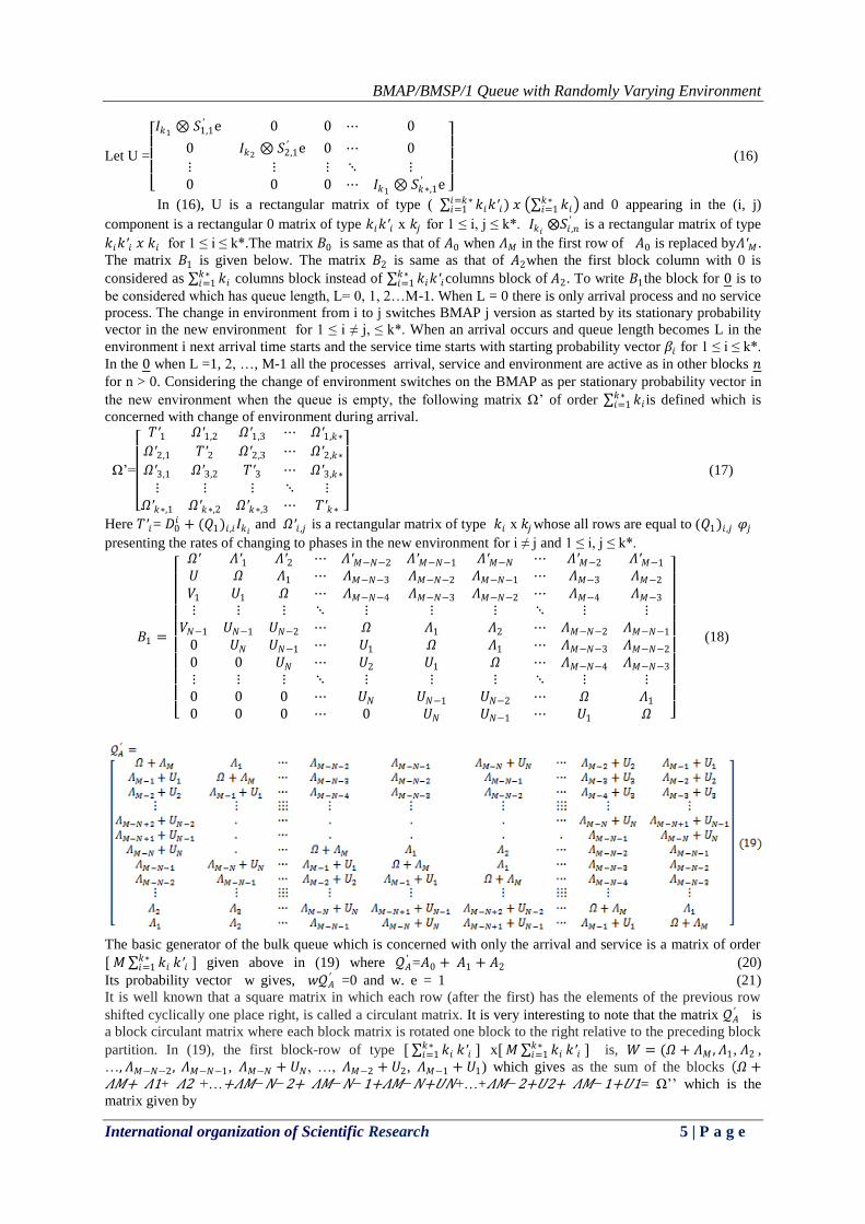
Let U =

𝐼𝑘1

⊗ 𝑆1,1′ e 0 0 ⋯ 0

0 𝐼𝑘2⊗ 𝑆2,1

′ e 0 ⋯ 0

⋮ ⋮ ⋮ ⋱ ⋮0 0 0 ⋯ 𝐼𝑘1

⊗ 𝑆𝑘∗,1′ e

(16)

In (16), U is a rectangular matrix of type ( 𝑘𝑖𝑘′𝑖𝑖=𝑘∗𝑖=1 ) 𝑥 𝑘𝑖

𝑘∗𝑖=1 and 0 appearing in the (i, j)

component is a rectangular 0 matrix of type 𝑘𝑖𝑘′𝑖 x 𝑘𝑗 for 1 ≤ i, j ≤ k*. 𝐼𝑘𝑖 ⨂𝑆𝑖 ,𝑛

′ is a rectangular matrix of type

𝑘𝑖𝑘′𝑖 𝑥 𝑘𝑖 for 1 ≤ i ≤ k*.The matrix 𝐵0 is same as that of 𝐴0 when 𝛬𝑀 in the first row of 𝐴0 is replaced by𝛬′𝑀 .

The matrix 𝐵1 is given below. The matrix 𝐵2 is same as that of 𝐴2when the first block column with 0 is

considered as 𝑘𝑖𝑘∗𝑖=1 columns block instead of 𝑘𝑖𝑘′𝑖

𝑘∗𝑖=1 columns block of 𝐴2. To write 𝐵1the block for 0 is to

be considered which has queue length, L= 0, 1, 2…M-1. When L = 0 there is only arrival process and no service

process. The change in environment from i to j switches BMAP j version as started by its stationary probability

vector in the new environment for 1 ≤ i ≠ j, ≤ k*. When an arrival occurs and queue length becomes L in the

environment i next arrival time starts and the service time starts with starting probability vector 𝛽𝑖 for 1 ≤ i ≤ k*.

In the 0 when L =1, 2, …, M-1 all the processes arrival, service and environment are active as in other blocks 𝑛

for n > 0. Considering the change of environment switches on the BMAP as per stationary probability vector in

the new environment when the queue is empty, the following matrix Ω’ of order 𝑘𝑖𝑘∗𝑖=1 is defined which is

concerned with change of environment during arrival.

Ω’=

𝑇′1 𝛺′1,2 𝛺′1,3 ⋯ 𝛺′1,𝑘∗

𝛺′2,1 𝑇′2 𝛺′2,3 ⋯ 𝛺′2,𝑘∗

𝛺′3,1 𝛺′3,2 𝑇′3 ⋯ 𝛺′3,𝑘∗

⋮ ⋮ ⋮ ⋱ ⋮𝛺′𝑘∗,1 𝛺′𝑘∗,2 𝛺′𝑘∗,3 ⋯ 𝑇′𝑘∗

(17)

Here 𝑇′𝑖= 𝐷0𝑖 + (𝑄1)𝑖 ,𝑖𝐼𝑘𝑖

and 𝛺′𝑖 ,𝑗 is a rectangular matrix of type 𝑘𝑖 x 𝑘𝑗 whose all rows are equal to (𝑄1)𝑖 ,𝑗 𝜑𝑗

presenting the rates of changing to phases in the new environment for i ≠ j and 1 ≤ i, j ≤ k*.

𝐵1 =

𝛺′ 𝛬′1 𝛬′2 ⋯ 𝛬′𝑀−𝑁−2 𝛬′𝑀−𝑁−1 𝛬′𝑀−𝑁 ⋯ 𝛬′𝑀−2 𝛬′𝑀−1

𝑈 𝛺 𝛬1 ⋯ 𝛬𝑀−𝑁−3 𝛬𝑀−𝑁−2 𝛬𝑀−𝑁−1 ⋯ 𝛬𝑀−3 𝛬𝑀−2

𝑉1 𝑈1 𝛺 ⋯ 𝛬𝑀−𝑁−4 𝛬𝑀−𝑁−3 𝛬𝑀−𝑁−2 ⋯ 𝛬𝑀−4 𝛬𝑀−3

⋮ ⋮ ⋮ ⋱ ⋮ ⋮ ⋮ ⋱ ⋮ ⋮𝑉𝑁−1 𝑈𝑁−1 𝑈𝑁−2 ⋯ 𝛺 𝛬1 𝛬2 ⋯ 𝛬𝑀−𝑁−2 𝛬𝑀−𝑁−1

0 𝑈𝑁 𝑈𝑁−1 ⋯ 𝑈1 𝛺 𝛬1 ⋯ 𝛬𝑀−𝑁−3 𝛬𝑀−𝑁−2

0 0 𝑈𝑁 ⋯ 𝑈2 𝑈1 𝛺 ⋯ 𝛬𝑀−𝑁−4 𝛬𝑀−𝑁−3

⋮ ⋮ ⋮ ⋱ ⋮ ⋮ ⋮ ⋱ ⋮ ⋮0 0 0 ⋯ 𝑈𝑁 𝑈𝑁−1 𝑈𝑁−2 ⋯ 𝛺 𝛬1

0 0 0 ⋯ 0 𝑈𝑁 𝑈𝑁−1 ⋯ 𝑈1 𝛺

(18)

The basic generator of the bulk queue which is concerned with only the arrival and service is a matrix of order

[ 𝑀 𝑘𝑖𝑘∗𝑖=1 𝑘′𝑖 ] given above in (19) where 𝒬𝐴

′ =𝐴0 + 𝐴1 + 𝐴2 (20)

Its probability vector w gives, 𝑤𝒬𝐴′ =0 and w. e = 1 (21)

It is well known that a square matrix in which each row (after the first) has the elements of the previous row

shifted cyclically one place right, is called a circulant matrix. It is very interesting to note that the matrix 𝒬𝐴′ is

a block circulant matrix where each block matrix is rotated one block to the right relative to the preceding block

partition. In (19), the first block-row of type [ 𝑘𝑖𝑘∗𝑖=1 𝑘′𝑖 ] x[ 𝑀 𝑘𝑖

𝑘∗𝑖=1 𝑘′𝑖 ] is, 𝑊 = (𝛺 + 𝛬𝑀 , 𝛬1, 𝛬2 ,

…, 𝛬𝑀−𝑁−2, 𝛬𝑀−𝑁−1, 𝛬𝑀−𝑁 + 𝑈𝑁, …, 𝛬𝑀−2 + 𝑈2, 𝛬𝑀−1 + 𝑈1) which gives as the sum of the blocks 𝛺 +𝛬𝑀+ 𝛬1+ 𝛬2 +…+𝛬𝑀−𝑁−2+ 𝛬𝑀−𝑁−1+𝛬𝑀−𝑁+𝑈𝑁+…+𝛬𝑀−2+𝑈2+ 𝛬𝑀−1+𝑈1= Ω’’ which is the

matrix given by



Ω’’=

𝚀′′1 𝛺1,2 𝛺1,3 ⋯ 𝛺1,𝑘∗

𝛺2,1 𝚀′′2 𝛺2,3 ⋯ 𝛺2,𝑘∗

𝛺3,1 𝛺3,2 𝚀′′3 ⋯ 𝛺3,𝑘∗

⋮ ⋮ ⋮ ⋱ ⋮𝛺𝑘∗,1 𝛺𝑘∗,2 𝛺𝑘∗,3 ⋯ 𝚀′′𝑘∗

(22)

where using (5) and (6), 𝑄’’𝑖 = (𝐷𝑖⨂𝐼𝑘′𝑖 ) + ( 𝐼𝑘𝑖⨂Si) + (𝑄1)𝑖 ,𝑖𝐼𝑘𝑖𝑘′𝑖

for 1 ≤ i ≤ k*. The stationary probability

vector of the basic generator given in (19) is required to get the stability condition. Consider the vector w = (

𝜋′1𝜑1 ⊗ 𝜙1, 𝜋′2𝜑2 ⊗ 𝜙2,…, 𝜋′𝑘∗𝜑𝑘∗ ⊗ 𝜙𝑘∗) where π’ = (𝜋′1 , 𝜋′2 , … , 𝜋′𝑘∗) is the stationary probability vector

of the environment, 𝜑𝑖 𝑎𝑛𝑑 𝜙𝑖 are the stationary probability vectors of the i version BMAP and i version BMSP

𝐷𝑖 and 𝑆𝑖respectively. It may be noted 𝜋′𝑖(𝜑𝑖 ⊗ 𝜙𝑖)[(𝐷𝑖⨂𝐼𝑘 ′𝑖) + ( 𝐼𝑘𝑖

⨂𝑆𝑖)] =0. This gives 𝜋′𝑖(𝜑𝑖 ⊗ 𝜙𝑖)𝑄’’𝑖 =

𝜋′𝑖(𝑄1)𝑖 ,𝑖 (𝜑𝑖 ⊗ 𝜙𝑖) 𝐼 = 𝜋′𝑖(𝑄1)𝑖 ,𝑖 (𝜑𝑖 ⊗ 𝜙𝑖) for 1 ≤ i ≤ k*. Now the first column of the matrix multiplication

of wΩ’’ is 𝜋′1(𝑄1)1,1𝜑1,1𝜙1,1 + 𝜋′2 (𝑄1)2,1𝜑11𝜙11[(𝜑2 ⊗ 𝜙2)𝑒] +.....+ 𝜋′𝑘∗ (𝑄1)𝑘∗,1𝜑11𝜙11[(𝜑𝑘∗ ⊗ 𝜙𝑘∗)]𝑒 = 0

since (𝜑𝑖 ⊗ 𝜙𝑖)𝑒 = 1 and π′𝑄1=0. In a similar manner it can be seen that the first column block of wΩ’’ is

𝜋′1(𝑄1)1,1𝜑1 ⊗ 𝜙1 + 𝜋′2 (𝑄1)2,1𝜑1 ⊗ 𝜙1[(𝜑2 ⊗ 𝜙2)𝑒] +.....+ 𝜋′𝑘∗ (𝑄1)𝑘∗,1𝜑1 ⊗ 𝜙1[(𝜑𝑘∗ ⊗ 𝜙𝑘∗)]𝑒 = 0 and i-

th column block is 𝜋′1(𝑄1)1,𝑖𝜑𝑖 ⊗ 𝜙𝑖[(𝜑1 ⊗ 𝜙1)𝑒] + 𝜋′2 (𝑄1)2,𝑖𝜑𝑖 ⊗ 𝜙𝑖[(𝜑2 ⊗ 𝜙2)𝑒] +.....+ 𝜋′𝑖 (𝑄1)𝑖 ,𝑖𝜑𝑖 ⊗

𝜙𝑖+ …+ 𝜋′𝑘∗ (𝑄1)𝑘∗,𝑖𝜑𝑖 ⊗ 𝜙𝑖[(𝜑𝑘∗ ⊗ 𝜙𝑘∗)]𝑒= 0. This shows that 𝑤 𝛺 + 𝛬𝑀 + 𝑤𝛬1+ 𝑤𝛬2 +…+𝑤𝛬𝑀−𝑁−2 + 𝑤𝛬𝑀−𝑁−1 + 𝑤𝛬𝑀−𝑁 + 𝑤𝑈𝑁+…+𝑤𝛬𝑀−2 + 𝑤𝑈2 + 𝑤𝛬𝑀−1 + 𝑤𝑈1= w Ω’’=0. So (w, w,…,w) .W= 0 = (w, w,

….w) W’ where W’ is the transpose W. This shows (w,w...w) is the left eigen vector of 𝒬𝐴′ and the

corresponding probability vector is w’ = 𝑤

𝑀,𝑤

𝑀,𝑤

𝑀, … . . ,

𝑤

𝑀 where w is given by

w = ( 𝜋′1(𝜑1 ⊗ 𝜙1), 𝜋′2(𝜑2 ⊗ 𝜙2),……, 𝜋′𝑘∗(𝜑𝑘∗ ⊗ 𝜙𝑘∗) ) (23)

Let 𝜑𝑖 = (𝜑𝑖 ,𝑗 ) and 𝜙𝑖 = (𝜙𝑖 ,𝑗 ) be the stationary probability components of the arrival and service processes.

Neuts [5], gives the stability condition as, w′ 𝐴0 𝑒 < 𝑤′ 𝐴2 𝑒 where w is given by (23). Taking the sum

cross diagonally in the 𝐴0 𝑎𝑛𝑑 𝐴2 matrices, it can be seen using (9) that

w’ 𝐴0 𝑒=1

𝑀 𝑤 𝑛𝛬𝑛

𝑀𝑛=1 𝑒 =

1

𝑀 𝑛𝑘∗

𝑖=1 𝜋′𝑖(𝜑𝑖 ⊗ 𝜙𝑖)(𝐷𝑛𝑖 ⊗ 𝐼𝑘 ′

𝑖)𝑒 𝑀

𝑛=1 = 1

𝑀 𝑛𝑘∗

𝑖=1 𝜋′𝑖(𝜑𝑖𝐷𝑛𝑖 𝑒 ⊗𝑀

𝑛=1

𝜙𝑖𝑒) =1

𝑀 𝜋′𝑖 𝜑𝑖( 𝑛𝑀

𝑛=1 𝐷𝑛𝑖 )𝑒 𝑘∗

𝑖=1 < 𝑤 ′𝐴2 𝑒 = 1

𝑀 𝑤 𝑛𝑈𝑛

𝑁𝑛=1 𝑒 =

1

𝑀 𝑛𝑘∗

𝑖=1 𝜋′𝑖(𝜑𝑖 ⊗ 𝜙𝑖)(𝐼𝑘𝑖 ⊗𝑁

𝑛=1

𝑆𝑛𝑖 )𝑒 =

1

𝑀 𝑛𝑘∗

𝑖=1 𝜋′𝑖(𝜑𝑖𝑒 ⊗ 𝜙𝑖𝑆𝑛𝑖 𝑒) 𝑁

𝑛=1 = 1

𝑀 𝜋′𝑖𝜙𝑖( 𝑛𝑁

𝑛=1 𝑆𝑛𝑖 )𝑒 𝑘∗

𝑖=1 . This gives the stability condition

as 𝜋′𝑖 𝜑𝑖( 𝑛𝑀𝑛=1 𝐷𝑛

𝑖 )𝑒𝑘∗𝑖=1 < 𝜋′𝑖

𝑘∗𝑖=1 𝜙𝑖 𝑛𝑁

𝑛=1 𝑆𝑛𝑖 𝑒 (24)

The sum 𝜑𝑖 ( 𝑛𝑀𝑛=1 𝐷𝑛

𝑖 )𝑒 and 𝜙𝑖 𝑛𝑁𝑛=1 𝑆𝑛

𝑖 𝑒 are known as the fundamental rates or the stationary rates of

arrival / service of the BMAP/ BMSP processes corresponding to the environment i for 1 ≤ i ≤ k*. This result

(24) is the stability condition for the random environment BMAP/BMSP/1 queue with random environment

where maximum arrival size is greater than the maximum service size. When (24) is satisfied, the stationary

distribution of the queue length exists Neuts [5]. Let π(0, i, j) : for 1 ≤ i ≤ k* 1 ≤ j ≤ 𝑘𝑖); π(0, k, i, j, j’) ; for 1 ≤

k ≤ M-1; 1 ≤ i ≤ k*; 1 ≤ j ≤ 𝑘𝑖 ; 1 ≤ j ≤ 𝑘′𝑖 and π(n, k, i, j, j’): for 0 ≤ k ≤ M-1; 1 ≤ i ≤ k*; 1 ≤ j ≤ 𝑘𝑖 ; 1 ≤ j ≤ 𝑘′𝑖 and n ≥ 1 be the stationary probability vectors of Markov chain X(t) states in (1) for this model.

Let 𝜋0=(π(0,1,1),π(0,1,2)…π(0,1,𝑘1),π(0,2,1),π(0,2,2)…π(0,2,𝑘2)…π(0,k*,1),π(0,k*,2)…π(0,k*,𝑘𝑘∗),

π(0,1,1,1,1),π(0,1,1,1,2)…π(0,1,1,𝑘1, 𝑘′1),π(0,1,2,1,1),π(0,1,2,1,2)…π(0,1,2,𝑘2, 𝑘′2),π(0,1,3,1,1),π(0,1,3,1,2)…

π(0,1,3,𝑘2 , 𝑘′2)…π(0,1,k*,1,1),π(0,1,k*,1,2)…π(0,1,k*,𝑘𝑘∗, 𝑘′𝑘∗),π(0,2,1,1,1)…π(0,2,k*,𝑘𝑘∗ , 𝑘′𝑘∗)…

π(0,M-1,1,1,1),π(0,M-1,1,1,2)…π(0,M-1,k*,𝑘𝑘∗ , 𝑘′𝑘∗)) be a vector of type 1x[ 𝑘𝑖𝑘∗𝑖=1 + (𝑀 − 1) 𝑘𝑖

𝑘∗𝑖=1 𝑘′𝑖].

Let 𝜋𝑛=(π(n,0,1,1,1),π(n,0,1,1,2)…π(n,0,1,𝑘1, 𝑘′1),π(n,0,2,1,1),π(n,0,2,1,2)…π(n,0,2,𝑘2, 𝑘′2),π(n,0,3,1,1),

π(n,0,3,1,2)…π(n,0,3,𝑘3 , 𝑘′3)…π(n,0,k*,1,1),π(n,0,k*,1,2)…π(n,0,k*,𝑘𝑘∗, 𝑘′𝑘∗),π(n,1,1,1,1),π(n,1,1,1,2)…

π(n,1,1,𝑘1 , 𝑘′1),π(n,1,2,1,1),π(n,1,2,1,2)…π(n,1,2,𝑘2, 𝑘′2),π(n,1,3,1,1),π(n,1,3,1,2)…π(n,1,3,𝑘3, 𝑘′3)…π(n,1,k*,1

,1),π(n,1,k*,1,2)…π(n,1,k*,𝑘𝑘∗, 𝑘′𝑘∗),π(n,2,1,1,1)…π(n,2,k*,𝑘𝑘∗ , 𝑘′𝑘∗),π(n,3,1,1,1)…π(n,3,k*,𝑘𝑘∗, 𝑘′𝑘∗)…

π(n,M-1,1,1,1),π(n,M-1,1,1,2)…π(n,M-1,k*,𝑘𝑘∗ , 𝑘′𝑘∗)) be a vector of type 1x[𝑀 𝑘𝑖𝑘∗𝑖=1 𝑘′𝑖]. The stationary

probability vector 𝜋 = (𝜋0 , 𝜋1 , 𝜋3, … ) satisfies the equations 𝜋𝑄𝐴=0 and πe=1. (25)

From (25), it can be seen 𝜋0𝐵1 + 𝜋1𝐵2=0. (26)

𝜋0𝐵0+𝜋1𝐴1+𝜋2𝐴2 = 0 (27)

𝜋𝑛−1𝐴0+𝜋𝑛𝐴1+𝜋𝑛+1𝐴2 = 0, for n ≥ 2. (28)

Introducing the rate matrix R as the minimal non-negative solution of the non-linear matrix equation

𝐴0+R𝐴1+𝑅2𝐴2=0, (29)

it can be proved (Neuts [5]) that 𝜋𝑛 satisfies the following. 𝜋𝑛 = 𝜋1 𝑅𝑛−1 for n ≥ 2. (30)

Using (26), 𝜋0 satisfies 𝜋0 = 𝜋1𝐵2(−𝐵1)−1 (31)

So using (27) and (31) and (30) the vector 𝜋1 can be calculated up to multiplicative constant since 𝜋1 satisfies

the equation 𝜋1 [𝐵2 −𝐵1 −1𝐵0 + 𝐴1 + 𝑅𝐴2] =0. (32)

Using (31) and (30) it can be seen that 𝜋1[𝐵2(−𝐵1)−1e+(I-R)−1𝑒] = 1. (33)



Replacing the first column of the matrix multiplier of 𝜋1 in equation (32), by the column vector multiplier of

𝜋1 in (33), a matrix which is invertible may be obtained. The first row of the inverse of that same matrix is 𝜋1

and this gives along with (31) and (30) all the stationary probabilities of the system. The matrix R is iterated

starting with 𝑅 0 = 0; and finding 𝑅 𝑛 + 1 = −𝐴0𝐴1−1–𝑅2(𝑛)𝐴2𝐴1

−1, for n ≥ 0. The iteration may be

terminated to get a solution of R at a norm level where 𝑅 𝑛 + 1 − 𝑅(𝑛 ) < ε.

2.3. Performance Measures of the System (i) The probability of the queue length S = r > 0, P(S=r) can be seen as follows. For 1 ≤ r ≤ M-1, P(S =r) =

𝜋(0, 𝑟, 𝑖, 𝑗1, 𝑗2𝑘′1𝑗2=1

𝑘𝑖𝑗1=1

𝑘∗𝑖=1 ). For r ≥ M, let n and k be non negative integers such that r = n M + k. Then

P(S=r) = 𝜋(𝑛, 𝑘, 𝑖, 𝑗1, 𝑗2𝑘′𝑖𝑗2=1

𝑘𝑖𝑗1=1

𝑘∗𝑖=1 ) , where r = n M + k, n ≥ 1 and k ≥ 0. (34)

(ii) The probability that the queue length is zero is P(S =0) = 𝜋 0, 𝑖, 𝑗 . 𝑘𝑖𝑗 =1

𝑘∗𝑖=1 (35)

(iii) The expected queue level E(S), can be calculated. Using (35) and (34), it may be seen that

E(S)= 𝑟∞0 𝑃(𝑆 = 𝑟)= 0𝜋 0, 𝑖, 𝑗

𝑘𝑖𝑗 =1

𝑘∗𝑖=1 + 𝑘𝜋(0, 𝑘, 𝑖, 𝑗1, 𝑗2

𝑘′𝑖𝑗2=1

𝑘𝑖𝑗1=1

𝑘∗𝑖=1 ) 𝑀−1

𝑘=1

+ 𝜋(𝑛, 𝑘, 𝑖, 𝑗1, 𝑗2𝑘′𝑖𝑗2=1

𝑘𝑖𝑗1=1

𝑘∗𝑖=1 )(𝑛𝑀 + 𝑘)𝑀−1

𝑘=0∞𝑛=1

= 𝑘𝜋(0, 𝑘, 𝑖, 𝑗1, 𝑗2𝑘′𝑖𝑗2=1

𝑘1𝑗1=1

𝑘∗𝑖=1 ) + 𝑀−1

𝑘=1 𝜋𝑛∞𝑛=1 .(Mn…Mn,Mn+1,…Mn+1,Mn+2,…Mn+2,…Mn+M-1,…

Mn+M-1)= 𝑘 𝜋(0, 𝑘 , 𝑖 , 𝑗 1, 𝑗 2𝑘′𝑖𝑗2=1

𝑘𝑖𝑗1=1

𝑘∗𝑖=1 ) + 𝑀−1

𝑘=1 M 𝑛𝜋𝑛∞𝑛=1 𝑒+𝜋1( 𝐼 − 𝑅)−1𝜉.

Here ξ= 0, … 0,1, … ,1,2, … ,2, … , 𝑀 − 1, … , 𝑀 − 1 ′ is of type [( 𝑘𝑖𝑘′𝑖)𝑘∗𝑖=1 M]x1 column vector

in which consecutively ( 𝑘𝑖𝑘′𝑖)𝑘∗𝑖=1 times 0,1,2,3..,M-1 appear. Let it be called ξ’ when 0 appears

( 𝑘 𝑖 )𝑘∗𝑖=1 times and others in that order appear ( 𝑘𝑖𝑘′𝑖)

𝑘∗𝑖=1 times. Then

E(S)= 𝜋0ξ’+ 𝜋1( 𝐼 − 𝑅)−1𝜉 + 𝑀𝜋1(𝐼 − 𝑅 )−2𝑒 (36)

(iv)Variance of S can be derived. Let η be column vector η=[0, . . ,0, 12, … 12 22, . . , 22, … 𝑀 − 1)2, … , (𝑀 − 1)2 ′ of type [( 𝑘𝑖𝑘′𝑖)

𝑘∗𝑖=1 M]x1in which consecutively ( 𝑘𝑖𝑘′𝑖)

𝑘∗𝑖=1 times squares of 0,1,2,3.., M-1 appear. Let it be

called η’ when 0 appears ( 𝑘𝑖)𝑘∗𝑖=1 times and others in the same manner as in η appear ( 𝑘𝑖𝑘′𝑖)

𝑘∗𝑖=1 times. Then

E(𝑆2)= 𝑟2∞0 𝑃(𝑆 = 𝑟)= 0𝜋 0, 𝑖, 𝑗

𝑘𝑖𝑗=1

𝑘∗𝑖=1 + 𝜋(0, 𝑘, 𝑖, 𝑗1, 𝑗2

𝑘′𝑖𝑗2=1

𝑘𝑖𝑗1=1

𝑘∗𝑖=1 )𝑘2 𝑀−1

𝑘=1

+ 𝜋(𝑛, 𝑘, 𝑖, 𝑗1, 𝑗2𝑘′𝑖𝑗2=1

𝑘𝑖𝑗1=1

𝑘∗𝑖=1 )(𝑛𝑀 + 𝑘)2𝑀−1

𝑘=0∞𝑛=1 =𝜋0η’ + 𝑀2 𝑛 𝑛 − 1 𝜋𝑛

∞𝑛=1 𝑒 + 𝑛𝜋𝑛

∞𝑛=1 𝑒 +

𝜋𝑛𝜂∞𝑛=1 + 2M 𝑛 𝜋𝑛

∞𝑛=1 𝜉.

So, E(𝑆2)= 𝜋0η’ + 𝑀2[𝜋1(𝐼 − 𝑅)−32𝑅 𝑒 + 𝜋1(𝐼 − 𝑅)−2𝑒] + 𝜋1(𝐼 − 𝑅)−1𝜂 + 2𝑀𝜋1(𝐼 − 𝑅)−2𝜉 (37)

VAR(S)=E(𝑆2) − [𝐸(𝑆)]2may be written from (36) and(37).

III. MODEL (B): MAXIMUM ARRIVAL SIZE M < MAXIMUM SERVICE SIZE N

The dual case of Model (A), namely the case, M < N is treated here. (When M =N both models are applicable

and one can use any one of them.) The assumption (vii) of Model (A) is changed and all its other assumptions

are retained.

3.1.Assumption

(vii) The maximum arrival size M= ma𝑥1≤𝑖≤𝑘∗𝑀𝑖 is less than the maximum service size

N=ma𝑥1≤𝑖≤𝑘∗𝑁𝑖 .

3.2.Analysis Since this model is dual, the analysis is similar to that of Model (A). The differences are noted below. The state

space of the chain is as follows presented in a similar way.

The state of the system of the continuous time Markov chain X (t) under consideration is presented as follows.

X(t) = {(0, i, j) : for 1 ≤ i ≤ k* 1 ≤ j ≤ 𝑘𝑖)} U {(0, k, i, j, j’) ; for 1 ≤ k ≤ N-1; 1 ≤ i ≤ k*; 1 ≤ j ≤ 𝑘𝑖 ; 1 ≤ j ≤ 𝑘′𝑖} U {(n, k, i, j, j’): for 0 ≤ k ≤ N-1; 1 ≤ i ≤ k*; 1 ≤ j ≤ 𝑘𝑖 ; 1 ≤ j ≤ 𝑘′𝑖 and n ≥ 1}. (38)

The chain is in the state (0, i, j) when the number of customers in the queue is 0, the environment state is i for

1 ≤ i ≤ k*and the arrival phase is j for 1 ≤ j ≤ 𝑘𝑖 . The chain is in the state (0, k, i, j, j’) when the number of

customers is k for 1 ≤ k ≤ N-1, the environment state is i for 1 ≤ i ≤ k*, the arrival phase is j for 1 ≤ j ≤ 𝑘𝑖 and

the service phase is j’ for 1 ≤ j’ ≤ 𝑘′𝑖 . The chain is in the state (n, k, i, j, j’) when the number of customers in the

queue is n N + k, for 0 ≤ k ≤ N-1 and 1 ≤ n < ∞, the environment state is i for 1 ≤ i ≤ k*, the arrival phase is j for

1 ≤ j ≤ 𝑘𝑖 and the service phase is j’ for 1 ≤ j’ ≤ 𝑘′𝑖 . When the number of customers waiting in the system is r,

then r is identified with (n, k) where r on division by N gives n as the quotient and k as the remainder. The

infinitesimal generator 𝑄𝐵 of the model has the same block partitioned structure given in (4) for Model (A) but

the inner matrices are of different orders.



𝑄𝐵 =

𝐵′

1 𝐵′0 0 0 . . . ⋯

𝐵′2 𝐴′

1 𝐴′0 0 . . . ⋯

0 𝐴′2 𝐴′

1 𝐴′0 0 . . ⋯

0 0 𝐴′2 𝐴′

1 𝐴′0 0 . ⋯

0 0 0 𝐴′2 𝐴′

1 𝐴′0 0 ⋯

⋮ ⋮ ⋮ ⋮ ⋱ ⋱ ⋱ ⋱

(39)

In (39) the states of the matrices are listed lexicographically as 0, 1, 2, 3, …. For partition purpose the zero states

in the first two sets of equation (38) are combined. The vector 0 is of type

1x[ 𝑘𝑖𝑘∗𝑖=1 + (𝑁 − 1) 𝑘𝑖

𝑘∗𝑖=1 𝑘′𝑖]with

0=((0,1,1),(0,1,2),(0,1,3)…(0,1, 𝑘1),(0,2,1),(0,2,2),(0,2,3)…(0,2, 𝑘2)…(0,k*,1),(0,k*,2),(0,k*,3)…(0,k*,𝑘𝑘∗),

(0,1,1,1,1),(0,1,1,1,2)…(0,1,1,1, 𝑘′1),(0,1,1,2,1),(0,1,1,2,2)...(0,1,1,2,𝑘′1),(0,1,1,3,1)...(0,1,1,3,𝑘′1)…(0,1,1,𝑘1,1)

…(0,1,1,𝑘1, 𝑘′1),(0,1,2,1,1),(0,1,2,1,2)…(0,1,2,1, 𝑘′2),(0,1,2,2,1),(0,1,2,2,2)….(0,1,2,2,𝑘′2),(0,1,2,3,1)....(0,1,2,3,

𝑘′2)…(0,1,2,𝑘2,1)…(0,1,2,𝑘2, 𝑘′2),(0,1,3,1,1)…(0,1,3,𝑘3, 𝑘′3)…(0,1,k*,1,1),…,(0,1,k*,𝑘𝑘∗, 𝑘′𝑘∗),(0,2,1,1,1),(0,2,

1,1,2)…(0,2,k*,𝑘𝑘∗,𝑘′𝑘∗),(0,3,1,1,1)…(0,3,k*,𝑘𝑘∗𝑘𝑘∗),(0,4,1,1,1)…(0,4,k*,𝑘𝑘∗𝑘′𝑘∗)…(0,N-1,1,1,1)…

(0,N-1,k*,𝑘𝑘∗, 𝑘′𝑘∗)) and the vector 𝑛 is of type 1x[𝑁 𝑘𝑖𝑘∗𝑖=1 𝑘′𝑖] and is given in a similar manner as follows

𝑛=(n,0,1,1,1),(n,0,1,1,2)...(n,0,1,1, 𝑘′1),(n,0,1,2,1)…(n,0,1,2,𝑘′1)…(n,0,k*,1,1)…(n,0,k*,𝑘𝑘∗, 𝑘′𝑘∗),(n,1,1,1,1)…

(n,1,k*,𝑘𝑘∗,𝑘′𝑘∗),(n,2,1,1,1)...(n,2,k*,𝑘𝑘∗,𝑘′𝑘∗)…(n,N-1,1,1,1),(n,N-1,1,1,2)…(n,N-1,k*,𝑘𝑘∗, 𝑘′𝑘∗)).

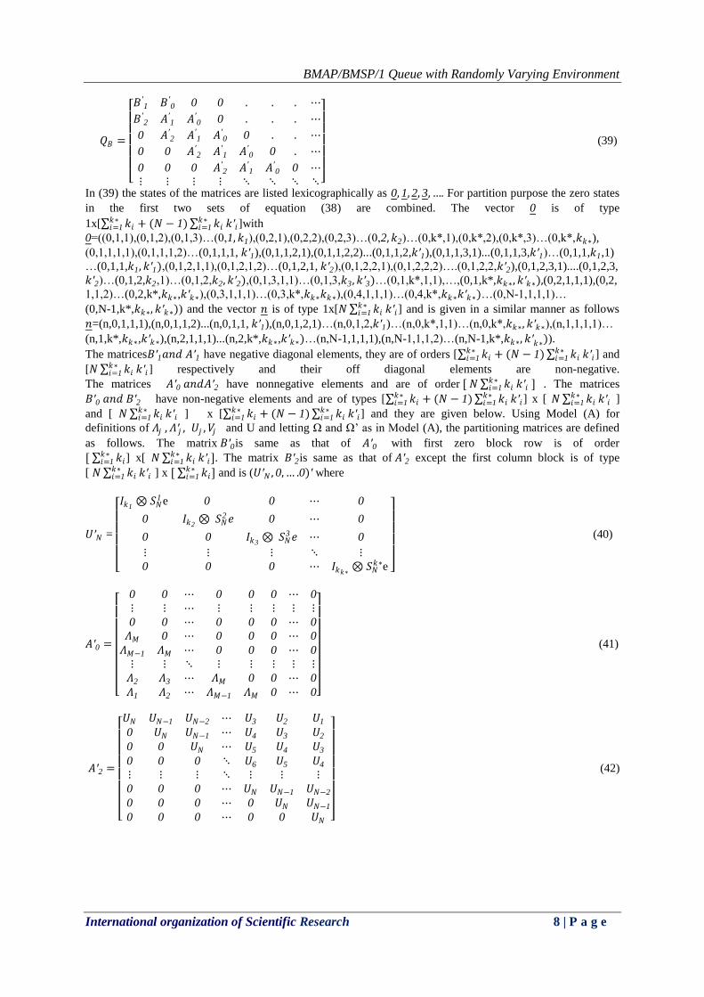
The matrices𝐵′1𝑎𝑛𝑑 𝐴′1 have negative diagonal elements, they are of orders [ 𝑘𝑖𝑘∗𝑖=1 + (𝑁 − 1) 𝑘𝑖

𝑘∗𝑖=1 𝑘′𝑖] and

[𝑁 𝑘𝑖𝑘∗𝑖=1 𝑘′𝑖 ] respectively and their off diagonal elements are non-negative.

The matrices 𝐴′0 𝑎𝑛𝑑𝐴′2 have nonnegative elements and are of order [ 𝑁 𝑘𝑖𝑘∗𝑖=1 𝑘′𝑖 ] . The matrices

𝐵′0 𝑎𝑛𝑑 𝐵′2 have non-negative elements and are of types [ 𝑘𝑖𝑘∗𝑖=1 + (𝑁 − 1) 𝑘𝑖

𝑘∗𝑖=1 𝑘′𝑖] x [ 𝑁 𝑘𝑖

𝑘∗𝑖=1 𝑘′𝑖 ]

and [ 𝑁 𝑘𝑖𝑘∗𝑖=1 𝑘′𝑖 ] x [ 𝑘𝑖

𝑘∗𝑖=1 + (𝑁 − 1) 𝑘𝑖

𝑘∗𝑖=1 𝑘′𝑖] and they are given below. Using Model (A) for

definitions of 𝛬𝑗 , 𝛬′𝑗 , 𝑈𝑗 , 𝑉𝑗 and U and letting Ω and Ω’ as in Model (A), the partitioning matrices are defined

as follows. The matrix 𝐵′0is same as that of 𝐴′0 with first zero block row is of order

[ 𝑘𝑖𝑘∗𝑖=1 ] x[ 𝑁 𝑘𝑖

𝑘∗𝑖=1 𝑘′𝑖]. The matrix 𝐵′2is same as that of 𝐴′2 except the first column block is of type

[ 𝑁 𝑘𝑖𝑘∗𝑖=1 𝑘′𝑖 ] x [ 𝑘𝑖

𝑘∗𝑖=1 ] and is (𝑈′𝑁 , 0, … .0)′ where

𝑈′𝑁 =

𝐼𝑘1

⊗ 𝑆𝑁1 e 0 0 ⋯ 0

0 𝐼𝑘2⊗ 𝑆𝑁

2 𝑒 0 ⋯ 0

0 0 𝐼𝑘3⊗ 𝑆𝑁

3 𝑒 ⋯ 0

⋮ ⋮ ⋮ ⋱ ⋮0 0 0 ⋯ 𝐼𝑘𝑘∗

⊗ 𝑆𝑁𝑘∗e

(40)

𝐴′0 =

0 0 ⋯ 0 0 0 ⋯ 0

⋮ ⋮ ⋯ ⋮ ⋮ ⋮ ⋮ ⋮0 0 ⋯ 0 0 0 ⋯ 0

𝛬𝑀 0 ⋯ 0 0 0 ⋯ 0

𝛬𝑀−1 𝛬𝑀 ⋯ 0 0 0 ⋯ 0

⋮ ⋮ ⋱ ⋮ ⋮ ⋮ ⋮ ⋮𝛬2 𝛬3 ⋯ 𝛬𝑀 0 0 ⋯ 0

𝛬1 𝛬2 ⋯ 𝛬𝑀−1 𝛬𝑀 0 ⋯ 0

(41)

𝐴′2 =

𝑈𝑁 𝑈𝑁−1 𝑈𝑁−2 ⋯ 𝑈3 𝑈2 𝑈1

0 𝑈𝑁 𝑈𝑁−1 ⋯ 𝑈4 𝑈3 𝑈2

0 0 𝑈𝑁 ⋯ 𝑈5 𝑈4 𝑈3

0 0 0 ⋱ 𝑈6 𝑈5 𝑈4

⋮ ⋮ ⋮ ⋱ ⋮ ⋮ ⋮0 0 0 ⋯ 𝑈𝑁 𝑈𝑁−1 𝑈𝑁−2

0 0 0 ⋯ 0 𝑈𝑁 𝑈𝑁−1

0 0 0 ⋯ 0 0 𝑈𝑁

(42)



𝐴′1 =

Ω 𝛬1 𝛬2 ⋯ 𝛬𝑀 0 0 ⋯ 0 0

𝑈1 Ω 𝛬1 ⋯ 𝛬𝑀−1 𝛬𝑀 0 ⋯ 0 0

𝑈2 𝑈1 Ω ⋯ 𝛬𝑀−2 𝛬𝑀−1 𝛬𝑀 ⋯ 0 0

⋮ ⋮ ⋮ ⋱ ⋮ ⋮ ⋮ ⋱ ⋮ ⋮𝑈𝑁−𝑀−1 𝑈𝑁−𝑀−2 𝑈𝑁−𝑀−3 ⋯ Ω 𝛬1 𝛬2 ⋯ 𝛬𝑀−1 𝛬𝑀

𝑈𝑁−𝑀 𝑈𝑁−𝑀−1 𝑈𝑁−𝑀−2 ⋯ 𝑈1 Ω 𝛬1 ⋯ 𝛬𝑀−2 𝛬𝑀−1

𝑈𝑁−𝑀+1 𝑈𝑁−𝑀 𝑈𝑁−𝑀−1 ⋯ 𝑈2 𝑈1 Ω ⋯ 𝛬𝑀−3 𝛬𝑀−2

⋮ ⋮ ⋮ ⋱ ⋮ ⋮ ⋮ ⋱ ⋮ ⋮𝑈𝑁−2 𝑈𝑁−3 𝑈𝑁−4 ⋯ 𝑈𝑁−𝑀−2 𝑈𝑁−𝑀−3 𝑈𝑁−𝑀−2 ⋯ Ω 𝛬1

𝑈𝑁−1 𝑈𝑁−2 𝑈𝑁−3 ⋯ 𝑈𝑁−𝑀−1 𝑈𝑁−𝑀−2 𝑈𝑁−𝑀−1 ⋯ 𝑈1 Ω

(43)

𝐵′1 =

𝛺′ 𝛬′1 𝛬′2 ⋯ 𝛬′𝑀 0 0 ⋯ 0 0

𝑈 Ω 𝛬1 ⋯ 𝛬𝑀−1 𝛬𝑀 0 ⋯ 0 0

𝑉1 𝑈1 Ω ⋯ 𝛬𝑀−2 𝛬𝑀−1 𝛬𝑀 ⋯ 0 0

⋮ ⋮ ⋮ ⋱ ⋮ ⋮ ⋮ ⋱ ⋮ ⋮𝑉𝑁−𝑀−2 𝑈𝑁−𝑀−2 𝑈𝑁−𝑀−3 ⋯ Ω 𝛬1 𝛬2 ⋯ 𝛬𝑀−1 𝛬𝑀

𝑉𝑁−𝑀−1 𝑈𝑁−𝑀−1 𝑈𝑁−𝑀−2 ⋯ 𝑈1 Ω 𝛬1 ⋯ 𝛬𝑀−2 𝛬𝑀−1

𝑉𝑁−𝑀 𝑈𝑁−𝑀 𝑈𝑁−𝑀−1 ⋯ 𝑈2 𝑈1 Ω ⋯ 𝛬𝑀−3 𝛬𝑀−2

⋮ ⋮ ⋮ ⋱ ⋮ ⋮ ⋮ ⋱ ⋮ ⋮𝑉𝑁−3 𝑈𝑁−3 𝑈𝑁−4 ⋯ 𝑈𝑁−𝑀−2 𝑈𝑁−𝑀−3 𝑈𝑁−𝑀−2 ⋯ Ω 𝛬1

𝑉𝑁−2 𝑈𝑁−2 𝑈𝑁−3 ⋯ 𝑈𝑁−𝑀−1 𝑈𝑁−𝑀−2 𝑈𝑁−𝑀−1 ⋯ 𝑈1 Ω

(44)

𝒬𝐵′′ =

𝛺 + 𝑈𝑁 𝛬1 + 𝑈𝑁−1 ⋯ 𝛬𝑀−1 + 𝑈𝑁−𝑀+1 𝛬𝑀 + 𝑈𝑁−𝑀 𝑈𝑁−𝑀−1 ⋯ 𝑈2 𝑈1

𝑈1 𝛺 + 𝑈𝑁 ⋯ 𝛬𝑀−2 + 𝑈𝑁−𝑀+2` 𝛬𝑀−1 + 𝑈𝑁−𝑀+1 𝛬𝑀 + 𝑈𝑁−𝑀 ⋯ 𝑈3 𝑈2

⋮ ⋮ ⋮⋮⋮ ⋮ ⋮ ⋮ ⋮⋮⋮ ⋮ ⋮𝑈𝑁−𝑀−2 𝑈𝑁−𝑀−3 ⋯ 𝛺 + 𝑈𝑁 𝛬1 + 𝑈𝑁−1 𝛬2 + 𝑈𝑁−2 ⋯ 𝛬𝑀 + 𝑈𝑁−𝑀 𝑈𝑁−𝑀−1

𝑈𝑁−𝑀−1 𝑈𝑁−𝑀−2 ⋯ 𝑈1 𝛺 + 𝑈𝑁 𝛬1 + 𝑈𝑁−1 ⋯ 𝛬𝑀−1 + 𝑈𝑁−𝑀+1 𝛬𝑀 + 𝑈𝑁−𝑀

𝛬𝑀 + 𝑈𝑁−𝑀 𝑈𝑁−𝑀−1 ⋯ 𝑈2 𝑈1 𝛺 + 𝑈𝑁 ⋯ 𝛬𝑀−2 + 𝑈𝑁−𝑀+2 𝛬𝑀−1 + 𝑈𝑁−𝑀+1

⋮ ⋮ ⋮⋮⋮ ⋮ ⋮ ⋮ ⋮⋮⋮ ⋮ ⋮𝛬2 + 𝑈𝑁−2 𝛬3 + 𝑈𝑁−3 ⋯ 𝑈𝑁−𝑀−1 𝑈𝑁−𝑀−2 𝑈𝑁−𝑀−3 ⋯ 𝛺 + 𝑈𝑁 𝛬1 + 𝑈𝑁−1

𝛬1 + 𝑈𝑁−1 𝛬2 + 𝑈𝑁−2 ⋯ 𝛬𝑀 + 𝑈𝑁−𝑀 𝑈𝑁−𝑀−1 𝑈𝑁−𝑀−2 ⋯ 𝑈1 𝛺 + 𝑈𝑁

(45)

The basic generator which is concerned with only the arrival and service is 𝑄𝐵′′ = 𝐴′0 + 𝐴′1 + 𝐴′2. This is also

block circulant. Using similar arguments given for Model (A) it can be seen that its probability vector is w’ =

𝑤

𝑁,𝑤

𝑁,𝑤

𝑁, … . . ,

𝑤

𝑁 where w is given by (23) and the stability condition remains the same. Following the

arguments given for Model (A), one can find the stationary probability vector for Model (B) also in matrix

geometric form. All performance measures including expectation of customers waiting for service and its

variance for Model (B) have the form as in Model (A) except M is replaced by N.

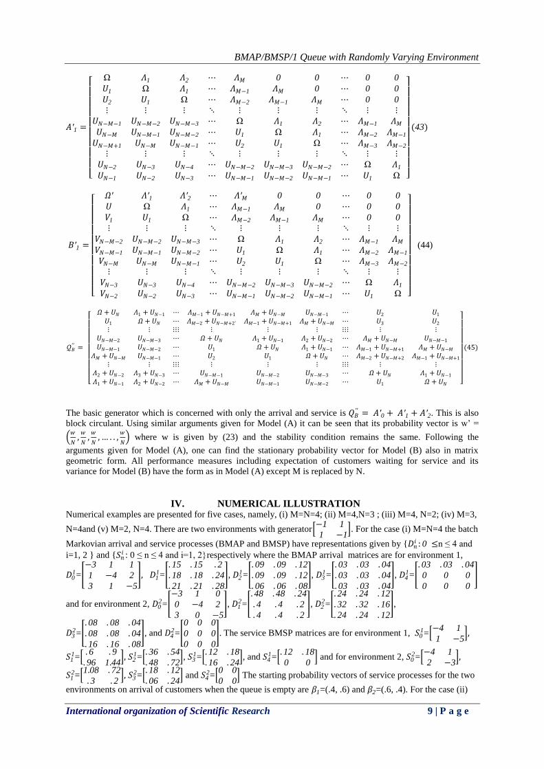
IV. NUMERICAL ILLUSTRATION Numerical examples are presented for five cases, namely, (i) M=N=4; (ii) M=4,N=3 ; (iii) M=4, N=2; (iv) M=3,

N=4and (v) M=2, N=4. There are two environments with generator −1 1

1 −1 . For the case (i) M=N=4 the batch

Markovian arrival and service processes (BMAP and BMSP) have representations given by {𝐷𝑛𝑖 : 0 ≤n ≤ 4 and

i=1, 2 } and {𝑆𝑛𝑖 : 0 ≤ n ≤ 4 and i=1, 2}respectively where the BMAP arrival matrices are for environment 1,

𝐷01=

−3 1 1

1 −4 2

3 1 −5

, 𝐷11=

. 15 . 15 . 2

. 18 . 18 . 24

. 21 . 21 . 28

, 𝐷21=

. 09 . 09 . 12

. 09 . 09 . 12

. 06 . 06 . 08

, 𝐷31=

. 03 . 03 . 04

. 03 . 03 . 04

. 03 . 03 . 04

, 𝐷41=

. 03 . 03 . 04

0 0 0

0 0 0

and for environment 2, 𝐷02=

−3 1 0

0 −4 2

3 0 −5

, 𝐷12=

. 48 . 48 . 24

. 4 . 4 . 2

. 4 . 4 . 2

, 𝐷22=

. 24 . 24 . 12

. 32 . 32 . 16

. 24 . 24 . 12

,

𝐷32=

. 08 . 08 . 04

. 08 . 08 . 04

. 16 . 16 . 08

, and 𝐷42=

0 0 0

0 0 0

0 0 0

. The service BMSP matrices are for environment 1, 𝑆01=

−4 1

1 −5 ,

𝑆11=

. 6 . 9

. 96 1.44 , 𝑆2

1= . 36 . 54

. 48 . 72 , 𝑆3

1= . 12 . 18

. 16 . 24 , and 𝑆4

1= . 12 . 18

0 0 and for environment 2, 𝑆0

2= −4 1

2 −3 ,

𝑆12=

1.08 . 72

. 3 . 2 , 𝑆3

2= . 18 . 12

. 06 . 24 and 𝑆4

2= 0 0

0 0 The starting probability vectors of service processes for the two

environments on arrival of customers when the queue is empty are 𝛽1=(.4, .6) and 𝛽2=(.6, .4). For the case (ii)



M=4, N=3 the above batch arrival and batch service rates (matrices) of case (i) are assumed except two service

rates matrices which are replaced as 𝑆31=

. 24 . 36

. 16 . 24 , and 𝑆4

1= 0 0

0 0 . For the case (iii) M=4, N=2 the above

batch arrival and batch service rates (matrices) of case (i) are assumed except the six service rates matrices

which are assumed as 𝑆21=

. 6 . 9

. 64 . 96 , 𝑆2

2= . 72 . 48

. 3 . 2 , 𝑆3

1=𝑆41=0 matrices and 𝑆3

2=𝑆42=0 matrices. For the case

(iv) M=3, N=4 the above batch arrival and batch service rates matrices of case (i) are assumed except two

arrival rates matrices which are replaced as 𝐷31=

. 06 . 06 . 08

. 03 . 03 . 04

. 03 . 03 . 04

and 𝐷41=

0 0 0

0 0 0

0 0 0

. For the case (v) M=2, N=4

the above batch arrival and batch service rates (matrices) of case (i) are assumed except the six arrival rates

matrices which are assumed as 𝐷21=

. 15 . 15 . 2

. 12 . 12 . 16

. 09 . 09 . 12

, 𝐷22=

. 32 . 32 . 16

. 4 . 4 . 2

. 4 . 4 . 2

, 𝐷31=𝐷4

1=0 matrices and 𝐷32=𝐷4

2=0

matrices. The partitioned matrices are of order 48, the rate matrix R is of order 48 and fifteen iterations are

performed to evaluate R matrix. The results obtained for various performance measures are tabulated in table 1.

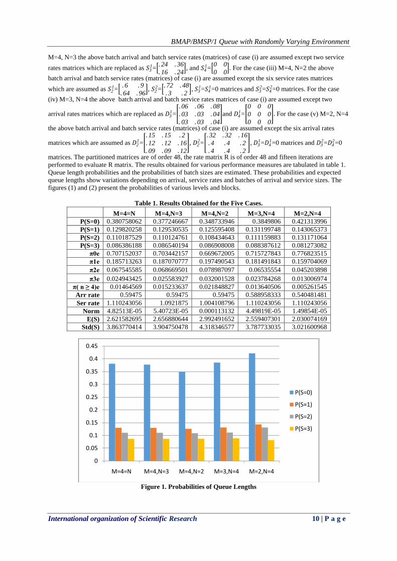
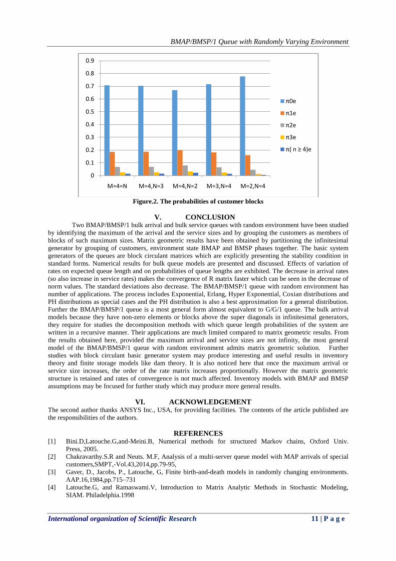
Queue length probabilities and the probabilities of batch sizes are estimated. These probabilities and expected

queue lengths show variations depending on arrival, service rates and batches of arrival and service sizes. The

figures (1) and (2) present the probabilities of various levels and blocks.

Table 1. Results Obtained for the Five Cases.

M=4=N M=4,N=3 M=4,N=2 M=3,N=4 M=2,N=4

P(S=0) 0.380758062 0.377246667 0.348733946 0.3849806 0.421313996

P(S=1) 0.129820258 0.129530535 0.125595408 0.131199748 0.143065373

P(S=2) 0.110187529 0.110124761 0.108434643 0.111159883 0.131171064

P(S=3) 0.086386188 0.086540194 0.086908008 0.088387612 0.081273082

π0e 0.707152037 0.703442157 0.669672005 0.715727843 0.776823515

π1e 0.185713263 0.187070777 0.197490543 0.181491843 0.159704069

π2e 0.067545585 0.068669501 0.078987097 0.06535554 0.045203898

π3e 0.024943425 0.025583927 0.032001528 0.023784268 0.013006974

π( n ≥ 4)e 0.01464569 0.015233637 0.021848827 0.013640506 0.005261545

Arr rate 0.59475 0.59475 0.59475 0.588958333 0.540481481

Ser rate 1.110243056 1.0921875 1.004108796 1.110243056 1.110243056

Norm 4.82513E-05 5.40723E-05 0.000113132 4.49819E-05 1.49854E-05

E(S) 2.621582695 2.656880644 2.992491652 2.559407301 2.030074169

Std(S) 3.863770414 3.904750478 4.318346577 3.787733035 3.021600968

Figure 1. Probabilities of Queue Lengths

0

0.05

0.1

0.15

0.2

0.25

0.3

0.35

0.4

0.45

M=4=N M=4,N=3 M=4,N=2 M=3,N=4 M=2,N=4

P(S=0)

P(S=1)

P(S=2)

P(S=3)



Figure.2. The probabilities of customer blocks

V. CONCLUSION Two BMAP/BMSP/1 bulk arrival and bulk service queues with random environment have been studied

by identifying the maximum of the arrival and the service sizes and by grouping the customers as members of

blocks of such maximum sizes. Matrix geometric results have been obtained by partitioning the infinitesimal

generator by grouping of customers, environment state BMAP and BMSP phases together. The basic system

generators of the queues are block circulant matrices which are explicitly presenting the stability condition in

standard forms. Numerical results for bulk queue models are presented and discussed. Effects of variation of

rates on expected queue length and on probabilities of queue lengths are exhibited. The decrease in arrival rates

(so also increase in service rates) makes the convergence of R matrix faster which can be seen in the decrease of

norm values. The standard deviations also decrease. The BMAP/BMSP/1 queue with random environment has

number of applications. The process includes Exponential, Erlang, Hyper Exponential, Coxian distributions and

PH distributions as special cases and the PH distribution is also a best approximation for a general distribution.

Further the BMAP/BMSP/1 queue is a most general form almost equivalent to G/G/1 queue. The bulk arrival

models because they have non-zero elements or blocks above the super diagonals in infinitesimal generators,

they require for studies the decomposition methods with which queue length probabilities of the system are

written in a recursive manner. Their applications are much limited compared to matrix geometric results. From

the results obtained here, provided the maximum arrival and service sizes are not infinity, the most general

model of the BMAP/BMSP/1 queue with random environment admits matrix geometric solution. Further

studies with block circulant basic generator system may produce interesting and useful results in inventory

theory and finite storage models like dam theory. It is also noticed here that once the maximum arrival or

service size increases, the order of the rate matrix increases proportionally. However the matrix geometric

structure is retained and rates of convergence is not much affected. Inventory models with BMAP and BMSP

assumptions may be focused for further study which may produce more general results.

VI. ACKNOWLEDGEMENT The second author thanks ANSYS Inc., USA, for providing facilities. The contents of the article published are

the responsibilities of the authors.

REFERENCES [1] Bini.D,Latouche.G,and-Meini.B, Numerical methods for structured Markov chains, Oxford Univ.

Press, 2005.

[2] Chakravarthy.S.R and Neuts. M.F, Analysis of a multi-server queue model with MAP arrivals of special

customers,SMPT,-Vol.43,2014,pp.79-95,

[3] Gaver, D., Jacobs, P., Latouche, G, Finite birth-and-death models in randomly changing environments.

AAP.16,1984,pp.715–731

[4] Latouche.G, and Ramaswami.V, Introduction to Matrix Analytic Methods in Stochastic Modeling,

SIAM. Philadelphia.1998

0

0.1

0.2

0.3

0.4

0.5

0.6

0.7

0.8

0.9

M=4=N M=4,N=3 M=4,N=2 M=3,N=4 M=2,N=4

π0e

π1e

π2e

π3e

π( n ≥ 4)e



[5] Neuts.M.F,Matrix-Geometric Solutions in Stochastic Models: An algorithmic Approach, The Johns

Hopkins Press, Baltimore,1981.

[6] Rama Ganesan, Ramshankar.R, and Ramanarayanan.R, M/M/1 Bulk Arrival and Bulk Service Queue

with Randomly Varying Environment,IOSR-JM,Vol.10,Issue6,Ver.III,2014,pp58-66.

[7] Sandhya.R, Sundar.V, Rama.G, Ramshankar.R and Ramanarayanan.R, M/M//C Bulk Arrival And Bulk

Service Queue With Randomly Varying Environment,IOSR-JEN,Vol.05,Issue02,||V1||,2015,pp.13-26.

[8] Ramshankar.R, Rama Ganesan, and Ramanarayanan.R PH/PH/1 Bulk Arrival and Bulk Service Queue,

IJCA,Vol.109,No.3,2015,pp.27-33.

[9] Ramshankar.R, Rama.G, Sandhya.R, Sundar.V and Ramanarayanan.R,(2015),PH/PH/1 Bulk Arrival and

Bulk Service Queue with Randomly Varying-Environment,-IOSRJEN,Vol.05.Issue02-||V4||.pp.01-12.

[10] Rama.G, Ramshankar.R, Sandhya.R, Sundar.V and Ramanarayanan.R, (2015),BMAP/M/C Bulk Service

Queue with Randomly Varying Environment, IOSRJEN, Vol.05, Issue 03,||V1||,pp.33-47.

[11] Lucantoni.D.M, (1993), Models and Techniques for Performance Evaluation of Computer and

Communication Systems,L. Donatiello and R. Nelson-Editors-Springer-verlag,,-pp330-358.

[12] Cordeiro and Kharoufch, J.P, Batch Markovian Arrival Processes (BMAP),www.dtic.mil/get-tr-

doc/pdf/AD=ADA536697&origin=publication-Detail.

[13] Qi-Ming-He,Fundamentals-of-Matrix-Analytic-Methods,Springer,2014.

[14] Rama Ganesan, and Ramanarayanan R, 2014, Stochastic Analysis of Project Issues and Fixing its Cause

by Project Team and Funding System Using-Matrix-Analytic-Method,IJCA,VOL.107,No.7,2014,pp.22-

28.

[15] Usha.K, Contribution to The Study of Stochastic Models in Reliability and Queues, Ph.D Thesis, 1981,

Annamlai University,India.

[16] Usha.K, The PH/M/C Queue with Varying Environment,Zastosowania Matematyki Applications

Mathematicae,XVIII,2 1984, pp.169-175.