D04452233

IOSR Journal of Engineering (IOSRJEN) www.iosrjen.org

ISSN (e): 2250-3021, ISSN (p): 2278-8719

Vol. 04, Issue 04 (April. 2014), ||V5|| PP 22-33

International organization of Scientific Research 22 | P a g e

Dynamic Modeling of Vehicles and Damper

Arshad Mehmood1, Ahmad Ali Khan

2, Ayaz Mehmood

3

1(Mechanical Engineering, Zakir Husain College of Engineering & Technology/AMU/INDIA) 2(Mechanical Engineering, Zakir Husain College of Engineering & Technology/AMU/INDIA)

3(Mechanical Engineering, Mewat Engineering College/MDU/INDIA)

Abstract: - The effect that the choice of suspension dampers has on a car‟s performance is an often misunderstood area. The increasing competitiveness of car category and the reduced opportunities for testing

mean that the team that can optimise their damper setup the quickest is likely to have a large advantage across

the entire usage. In the past the selection of dampers was done empirically. The increasing availability of

computational power means that numerical simulation is now a viable method of optimising a vehicle before it arrives at the track. This paper outlines the development of the equations of motion for some simple vehicle

models. It then demonstrates how these equations can be solved to estimate the road holding performance of a

race car.

Although results for one particular vehicle have been studied, the focus throughout is to demonstrate numerical

and computational techniques that can be used to optimise car‟s dampers. A degree of generality has been

maintained while analysing these techniques so that they can be applied to a variety of different categories of car

models.

I. INTRODUCTION To maximise road holding, a car‟s suspension must allow its tyres to follow the road profile. This is

often achieved by using what is known as „soft‟ suspension, or using shock absorbers that employ a low damping coefficient. Another consideration in maximising the road holding of a vehicle is to minimise the body

roll of the chassis. Typically, this can be achieved by employing „hard‟ suspension with higher damping

coefficients. Both of these techniques are aimed at reducing the load fluctuations Most modern race cars employ

dampers with non linear characteristics, which are often specified on a graph of force versus velocity, known as

the damper curve. These are non-linear, in that they usually employ two different damping coefficients, one in

the low velocity region of the curve, and another in the high speed region. Typically, these will have a higher

damping coefficient at low velocities where body roll tends to occur, and a lower damping coefficient at higher

velocity, where road disturbances tend to occur [1]. The damping coefficient is also often higher in rebound,

which occurs as the damper is extending. between the tyre and the road. These adjustments can be made

independently for each of the four dampers on the vehicle. This paper aims to select the most appropriate values

for each of these four adjustable parameters. It also aims to outline a method of estimating the optimal damper

characteristics, which can be used by car before they even arrive at the track, and also to account for the changes in the vehicle‟s setup due to changing track conditions [2]. This will therefore give these teams a big advantage

for the entire motion.

The primary role of a damper on a vehicle is to oppose the undesirable motions of the suspended vehicle body

and to control the oscillation of the sprung masses. As one of the most fundamental contributors to a vehicle‟s

handling, dampers have been studied at great length. This began with the introduction of internal combustion

engine driven vehicles in the late nineteenth century [3], when the increased speed available due to these

engines made an undamped vehicle inherently unsafe. Since this time, dampers have undergone a number of

significant transformations.

In modern vehicles, there are two major classifications of dampers, passive and active dampers. Passive

damping systems function with fixed operating characteristics, such as damping coefficient. Although these

characteristics may be nonlinear and can sometimes be adjusted by the operator, they will not change in real-time to adjust to the road conditions or the behaviour of a vehicle. This is in contrast to an active suspension

system, where an adaptive control system is used to ensure that the optimum damping force is produced in real

time.

A historical review of the development of active and semiactive suspension systems is presented by Karnopp

[4]. Passive damping systems are still the more common system, used on most family vehicles and even a large

majority of cars.

As explained by Nowlan [5], some assumptions may be made. These are:

• The damping of the tyre is negligible

• The spring rate of the tyre is much higher than the spring rate of the suspension elements

• The sprung mass of the vehicle body is much higher than the unsprung mass of the wheel and axle.



II. MODELLING OF QUARTER CAR MODEL Although for most practical purposes, the single degree of freedom vehicle representation is too

simplistic to be completely meaningful, its results, and the method of derivation of these results are a necessary

building block when studying more complicated systems [6]. The next simplest model to study is the two degree of freedom system given in Figure 1. This is also known as the quarter car model, as it may be thought of a

representing the dynamics of a quarter of the car (for example, the front left quarter). The advantage of the Two-

Degree of freedom quarter car model is that while still a relatively simple system to analyse, it allows a good

approximation of the motion of both the chassis and the wheels of a vehicle.

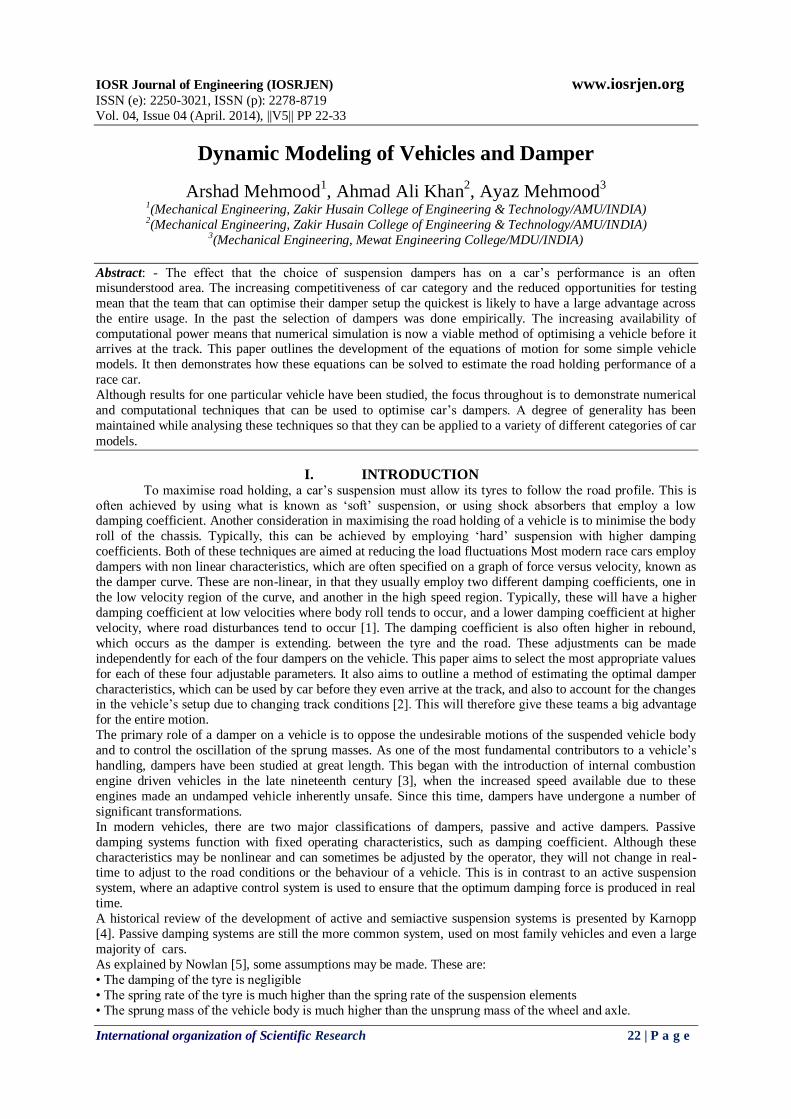
Figure 1 Free body diagram for a Two-Degree of freedom quarter car model

2.1. Governing Equation of Motion

Using Newton‟s second law of motion, the equations of motion for the system shown in Figure 3.1, becomes:

)()()()( sussusurturtuu xxcxxkxxcxxkxm

)()( sussusss xxcxxkxM

Assuming harmonic motion of base and the masses

surieXtx tj

ii ,, ; )(

where Xi is the amplitude of harmonic motion

0

)()(2

2rtt

s

u

sssss

ssststuxcjk

x

x

jckMjck

jckccjkkm

The frequency response function (FRF) of the sprung mass of the quarter car model may be defined as the ratio

of magnitude of sprung mass to the road profile, as given by;

r

ss

x

xH )(

And the frequency response function of the unsprung mass of the quarter car model may be defined as the ratio

of magnitude of unsprung mass to the road profile, as given by;

r

us

x

xH )(

0

)()(

rtt

s

u xcjk

x

xA

each side of the equation are multiplied by the inverse of A, we get

0

)(11 rtt

s

u xcjkA

x

xAA



0

)(

)(det

1 2

2

rtt

st

stu

ss

sssss

s

u

xcjk

cc

jkkmjck

jckjckM

A

x

x

equation (5.11) becomes

))((

)(

det

12

ttss

ttsss

s

u

cjkjck

cjkjckM

Ax

x

where:

222 )(det jckjckMccjkkmA sssssststu there by resulting in

the frequency response functions of the two degrees of freedom given by equation

2

2 2

( )

( )( )

( ( ))

( ) ( )

s s

t ts

u t s t s

s s s s s

k c j

k j cH

m k k j c c

M k c j k c j

…. 1

2

2

2 2

( )

( )( )

( ( ))

( ) ( )

s s s

t tu

u t s t s

s s s s s

M k c j

k j cH

m k k j c c

M k c j k c j

2

0 5 10 150.2

0.4

0.6

0.8

1

1.2

1.4

1.6

Frequency of Base Excitation (Hz)

Tra

nsm

issib

ility

Ratio of amplitude of unsprung mass to amplitude of road profile

Damping Ratio = 0.62




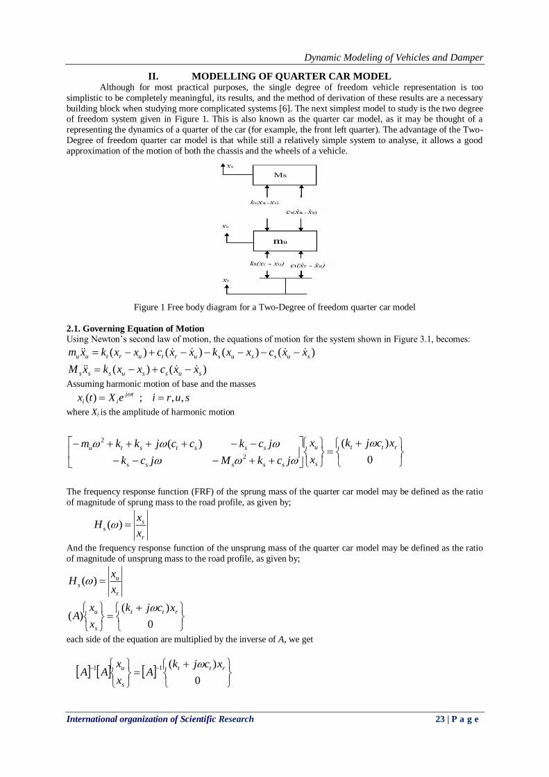
Figure 2 Frequency response function of the unsprung mass of the quarter car model

The frequency response functions show the ratio of magnitude of output displacement versus the

input displacement. In this case the output displacement can be of any degrees of freedom of the system being

studied. The input to the system is the amplitude of road profile fluctuations. Figure 2 shows the frequency

response function of the unsprung mass for the two-degree of freedom quarter car model. Several different

damping ratios have been plotted on the same axes to illustrate how the behaviour of the car may change due to

different damping ratios. It is clearly visible in this graph that even a small change in damping ratio, from 0.46

to 1.09, can have a very drastic effect on the motion of the unsprung mass [7]. In the frequency range between 0 and approximately 3 Hz, the different damping ratios have very little effect. In the region approximately

between 2 to 6 Hz, the lower damping ratio (of 0.62) will result in lower amplitude of displacement of the

unsprung mass. In contrast, in the region beyond 6 Hz, the higher damping ratio of 1.09 will result in less



displacement of the unsprung mass. It can also be observed from this with the higher damping ratios there is a

single local maximum for the FRF curve. Lowering the damping ratio may add a second local maximum at

approximately 7 Hz, and the height of this increases as the amount of damping in the system decreases.

0 5 10 150

0.5

1

1.5


Transm

issib

ility

Ratio of amplitude of sprung mass to amplitude of road profile





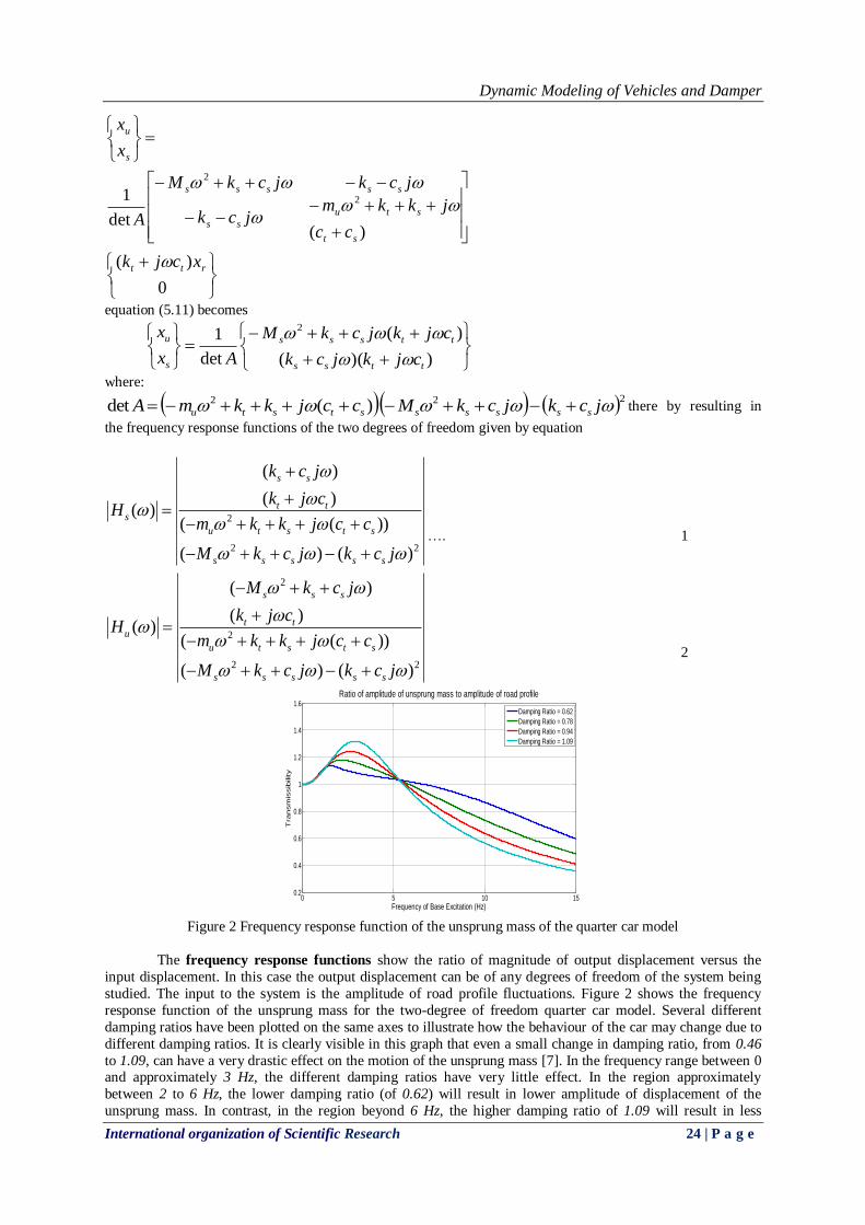
Figure 3 Frequency response function of the sprung mass of the quarter car model

The frequency response function of the sprung mass of the quarter car model is shown in Figure 3. It

can be seen that there is a single peak in the FRF for all of the damping ratios examined. This peak occurs at

approximately at the same frequency that is 2Hz regardless of the amount of damping applied. One important

factor to note is that the lower the damping ratio, the higher the peak amplitude of the FRF. That is, that if the

vehicle is subjected to random broadband input, most of the motion of the sprung mass will occur at a low

frequency, and in order to control the movement of the sprung mass, a higher damping ratio is required.

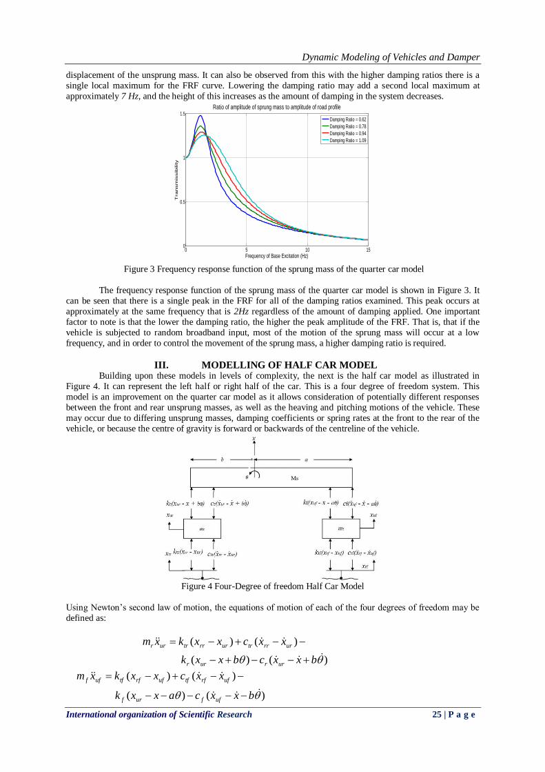
III. MODELLING OF HALF CAR MODEL Building upon these models in levels of complexity, the next is the half car model as illustrated in

Figure 4. It can represent the left half or right half of the car. This is a four degree of freedom system. This

model is an improvement on the quarter car model as it allows consideration of potentially different responses

between the front and rear unsprung masses, as well as the heaving and pitching motions of the vehicle. These

may occur due to differing unsprung masses, damping coefficients or spring rates at the front to the rear of the

vehicle, or because the centre of gravity is forward or backwards of the centreline of the vehicle.

Figure 4 Four-Degree of freedom Half Car Model

Using Newton‟s second law of motion, the equations of motion of each of the four degrees of freedom may be

defined as:

)()(

)()(

bxxcbxxk

xxcxxkxm

urrurr

urrrtrurrrtrurr

)()(

)()(

bxxcaxxk

xxcxxkxm

uffurf

ufrftfufrftfuff



)()(

)()(

bxxcaxxk

bxxcbxxkxM

fuffuf

urrurrs

)()(

)()(

bxxacaxxak

bxxbcbxxbkJ

fuffuf

urrurr

Equations may be separated into their output and input components

r ur tr ur tr ur r ur r r

r ur r r tr rr tr rr

m x k x c x k x k x k b

c x c x c b k x c x

f uf tf uf tf uf f uf f f

f uf f f tf rf tf rf

m x k x c x k x k x k a

c x c x c a k x c x

0

s r ur r r r ur r r

f uf f f f uf f f

M x k x k x k b c x c x c b

k x k x k a c x c x c a

2 2

2 2 0

r ur r r r ur r r f uf

f f f uf f f

J k bx k bx k b c bx c bx c b k ax

k ax k a c ax c ax c a

Assuming that the input displacements, and hence the motion of each of the degrees of freedom is harmonic; tj

ii eXtx )(

where, 2

11 ( )r tr r tr ra m k k j c c

2

22 ( )f tf f tf fa m k k j c c

(5.28)

2

33 ( )s r f r fa M k k j c c

2 2 2 2 2

44 ( )r f r fa J k b k a j c b c a

= 0

31 13 r ra a k j c

41 14 r ra a k b j c b

23 32 f fa a k j c

24 42 f fa a k a j c a

34 43 ( )r f f ra a k b k a j c a c b

The motions xrr and xrf refer to the irregularity of the road profile, because both wheels are driving over the same

piece of road, it is assumed that xrf is equal to xrr.

trtr cjkf 1

tftf cjkf 2

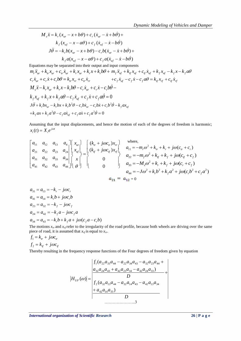
Thereby resulting in the frequency response functions of the Four degrees of freedom given by equation

D

aaa

aaaaaaaaaf

D

aaaaaaaaa

aaaaaaaaaf

HUF

)

(

)

(

)(

331442

3413424314324413322

332442342342432432

4423324334224433221

…………………..3

11 12 13 4

21 22 23 24

31 32 33 34

41 42 43 44

( )

( )

0

0

ur tr tr rr

uf tf tf rf

a a a a x k j c x

x k j c xa a a a

a a a a x

a a a a



D

aaa

aaaaaaaaaf

D

aaa

aaaaaaaaa

aaaaaaaaaf

HUR

)

(

)

(

)(

332441

3423414324314423311

331441

341341431431441331

4413314334114433112

…………..4

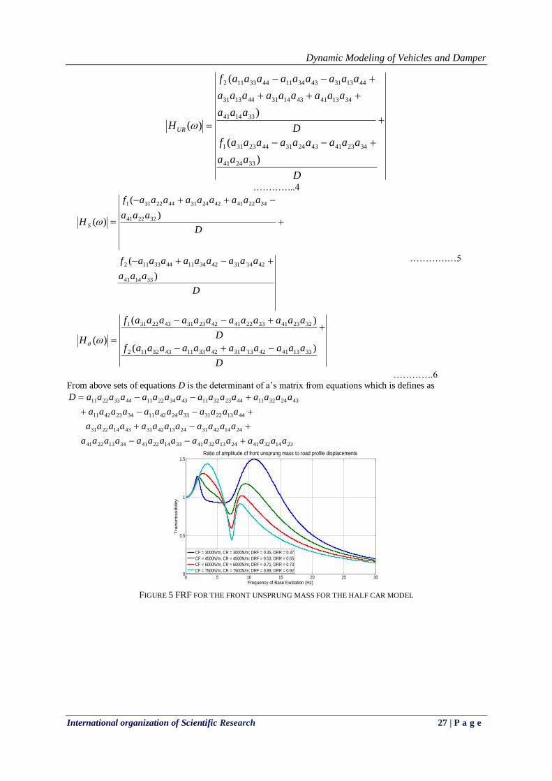
D

aaa

aaaaaaaaaf

D

aaa

aaaaaaaaaf

H S

)

(

)

(

)(

331441

4214`314234114433112

322241

3422414224314422311

……………5

D

aaaaaaaaaaaaf

D

aaaaaaaaaaaaf

H)(

)(

)(3313414213`314233114332112

3223413322414223314322311

………….6

From above sets of equations D is the determinant of a‟s matrix from equations which is defines as

23143241241332413314224134132241

241442312413423143142231

441322313324421134234211

43243211442332114334221144332211

aaaaaaaaaaaaaaaa

aaaaaaaaaaaa

aaaaaaaaaaaa

aaaaaaaaaaaaaaaaD

0 5 10 15 20 25 300

0.5

1

1.5


Tra

nsm

issib

ility

Ratio of amplitude of front unsprung mass to road profile displacements

CF = 3000N/m, CR = 3000N/m; DRF = 0.35, DRR = 0.37

CF = 4500N/m, CR = 4500N/m; DRF = 0.53, DRR = 0.55

CF = 6000N/m, CR = 6000N/m; DRF = 0.71, DRR = 0.73

CF = 7500N/m, CR = 7500N/m; DRF = 0.89, DRR = 0.92

FIGURE 5 FRF FOR THE FRONT UNSPRUNG MASS FOR THE HALF CAR MODEL



0 5 10 15 20 25 300

0.2

0.4

0.6

0.8

1

1.2

1.4

1.6

1.8


Transm

issib

ility

Ratio of amplitude of rear unsprung mass to road profile displacements

CF = 3000N/m, CR = 3000N/m; DRF = 0.35, DRR = 0.37

CF = 4500N/m, CR = 4500N/m; DRF = 0.53, DRR = 0.55

CF = 6000N/m, CR = 6000N/m; DRF = 0.71, DRR = 0.73

CF = 7500N/m, CR = 7500N/m; DRF = 0.89, DRR = 0.92

Figure 6 FRF for the front unsprung mass for the half car model

0 5 10 15 20 25 300

0.5

1

1.5

2

2.5

3


Tra

nsm

issib

ility

Ratio of amplitude of heave to road profile displacements

CF = 3000N/m, CR = 3000N/m; DRF = 0.35, DRR = 0.37

CF = 4500N/m, CR = 4500N/m; DRF = 0.53, DRR = 0.55

CF = 6000N/m, CR = 6000N/m; DRF = 0.71, DRR = 0.73

CF = 7500N/m, CR = 7500N/m; DRF = 0.89, DRR = 0.92


0 5 10 15 20 25 300

0.1

0.2

0.3

0.4

0.5

0.6

0.7


Transm

issib

ility

Ratio of amplitude of pitch profile to road profile displacements

CF = 3000N/m, CR = 3000N/m; DRF = 0.35, DRR = 0.37

CF = 4500N/m, CR = 4500N/m; DRF = 0.53, DRR = 0.55

CF = 6000N/m, CR = 6000N/m; DRF = 0.71, DRR = 0.73

CF = 7500N/m, CR = 7500N/m; DRF = 0.89, DRR = 0.92


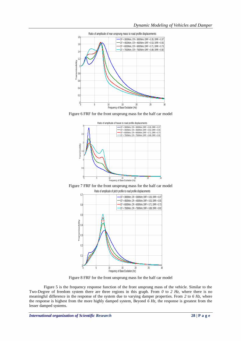
Figure 5 is the frequency response function of the front unsprung mass of the vehicle. Similar to the

Two-Degree of freedom system there are three regions in this graph. From 0 to 2 Hz, where there is no

meaningful difference in the response of the system due to varying damper properties. From 2 to 6 Hz, where

the response is highest from the more highly damped system, Beyond 6 Hz, the response is greatest from the

lesser damped systems.



The response of the rear unsprung mass also follows similar pattern, as shown in Figure 6. It should be

noted that the only difference in the model between the front and rear of the vehicle is the mass distribution that

is the unsprung mass of the rear wheels is higher and the unsprung mass at the front wheel is lower compared to

the front of the car. This affects not only the magnitude of the displacements of the unsprung masses, but also

the damped natural frequencies, where these peaks occur.

Figure 7 and Figure 8 shows the frequency response functions for the heave and pitch modes of the sprung mass of the system respectively. The heave mode is the vertical displacement of the sprung mass, while

the pitch mode refers to its angular displacement. The heave mode of the sprung mass of the Four-Degree of

freedom system is very similar in meaning to the sprung mass of the Two-Degree of freedom quarter car model

shown in Figure 1, and the frequency response functions confirm the same. In both cases, the peaks occur at

approximately the same frequency. Also in both cases, the lower damping coefficients result in higher peak

transmissibility, and the effect of this can be profound. Although it may be observed from Figure 4 that

increasing the damping coefficients of the system will reduce the value of the peak heave response, it is evident

from Figure 5.6 that the opposite is true when it comes to the pitching motion of the sprung mass.That is,

increasing the damping coefficients of the system will increase the peak pitching response of the vehicle.

Obviously, it is necessary to reach a compromise between these conflicting parameters.

IV. TYRE LOAD FLUCTUATIONS The performance of a car tyre is inversely proportional to the variation of its contact force with the road. There

have been many attempts at quantifying the effect of tyre load fluctuations. The evaluation criterion for the

quarter car load fluctuation rate Ru as being,

gmM

kR

us

tu

)(

This equation allows a quantitative analysis of the effect of varying the vehicle parameters. By minimising the value of Rs (or in the more general case R), the vehicle that has the lowest tyre load fluctuations

can be considered. This will result in higher average traction available to the tyres. Obtaining the values of xr and

xu in this equation depends on not only the FRF of the system, but also requires some information about the

shape of the road profile. This is usually given in the form of a power spectral density of the size of the road

profile irregularities.

4.1 Power spectral density

In order to make quantitative comparisons between different vehicle setups, it is necessary to have a

realistic profile of the road surface characteristics [8]. This is most conveniently done by plotting the magnitude

of displacement of the road profile in the frequency domain. This is known as the power spectral density (PSD)

of the road surface. There have been many different attempts for creating a general PSD model for road profiles, and these have been studied at length.

The comparison is to be made of the performance of the same vehicle with several different dampers

over a generic stretch of road. Therefore, any realistic approximation of the PSD of the road profile will provide

sufficient results to make a comparison between these different damper set-ups. Care must be taken in the

interpretation of these results however, as cars are required to compete on roads with varying roughness and

bump characteristics. The most appropriate damper for one PSD road profile is not necessarily the best for

another road.

Another complicating factor is that most approximations of road profile are given in terms of spatial

frequency of the road profile disturbances. Spatial frequency is the inverse of the wavelength. It may be thought

of as the number of cycles or road profile fluctuations per distance travelled. The number of fluctuations per

second is therefore dependent upon the velocity of the vehicle across this road profile. In order to convert spatial

frequency into radian frequency, it is necessary to multiply the special frequency by 2πv, where v is the velocity of the vehicle. The velocity of car is not constant and can vary anywhere up to 70kilometres per hour. The PSD

used by Tamboli et al will be used, as it simplifies the problem somewhat by assuming a constant velocity. This

PSD is defined as:

)()( bfaefG

where,

a: describes the general roughness of the road.

b: describes the wavelength distribution.

f: refers to frequency (Hz)



Tamboli et al [9] suggests the coefficients for PSD obtained in Table 1. These values are dependent upon both

the quality of the road, and also the speed of the vehicle travelling on it. However the highway driving is likely

to be the better approximation of the two, and will therefore be used for comparing the different dampers.

Table 1 Coefficients of the PSD used by Tamboli

Road type a (m2/Hz) b

Highway 4.85 × 10-4 0.19

City 23.0244 × 10-4 0.213

The mean square displacement of the road irregularities may be found from the PSD:

0

2

)( dffGx …………7

Equation (7) may be discretised to find the root mean square displacements in a given frequency band:

2

2

, )(

hf

hf

fr

n

n

ndffGx …………8

where,

fn = the centre frequency of the frequency band.

ℎ = the width of the frequency band.

Equation (8) may be used to represent the amplitude of displacement, or irregularity of the road profile

within each given frequency band [10]. The mean value of the actual response of the vehicle must relate the

amplitude of the road profile fluctuations to the frequency response of the vehicle in that same frequency band.

The mean value of the FRF in each frequency band is given by.

2

2

)(1

hf

hf

f

n

n

ndfH

hH

where ω =2πf

The amplitude of displacement of the unsprung mass can now be calculated for each frequency band using following relation,

nnn ffrfu Hxx ,, ………9

Equations (7) and (8) can now be substituted into equation (9) and be rewritten as it is in equation (10). All of

the information required to obtain the load fluctuation rate Ru of the vehicle is

……10

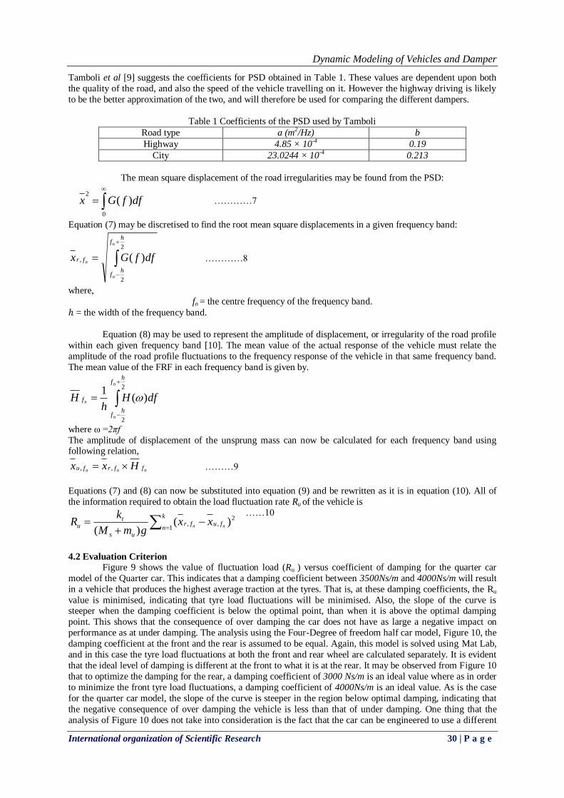
4.2 Evaluation Criterion Figure 9 shows the value of fluctuation load (Ru ) versus coefficient of damping for the quarter car

model of the Quarter car. This indicates that a damping coefficient between 3500Ns/m and 4000Ns/m will result

in a vehicle that produces the highest average traction at the tyres. That is, at these damping coefficients, the Ru

value is minimised, indicating that tyre load fluctuations will be minimised. Also, the slope of the curve is steeper when the damping coefficient is below the optimal point, than when it is above the optimal damping

point. This shows that the consequence of over damping the car does not have as large a negative impact on

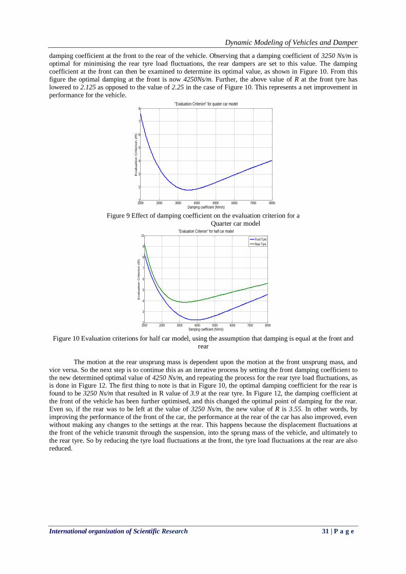
performance as at under damping. The analysis using the Four-Degree of freedom half car model, Figure 10, the

damping coefficient at the front and the rear is assumed to be equal. Again, this model is solved using Mat Lab,

and in this case the tyre load fluctuations at both the front and rear wheel are calculated separately. It is evident

that the ideal level of damping is different at the front to what it is at the rear. It may be observed from Figure 10

that to optimize the damping for the rear, a damping coefficient of 3000 Ns/m is an ideal value where as in order

to minimize the front tyre load fluctuations, a damping coefficient of 4000Ns/m is an ideal value. As is the case

for the quarter car model, the slope of the curve is steeper in the region below optimal damping, indicating that

the negative consequence of over damping the vehicle is less than that of under damping. One thing that the

analysis of Figure 10 does not take into consideration is the fact that the car can be engineered to use a different

2,

1, )(

)(nn fu

k

nfr

us

tu xx

gmM

kR



damping coefficient at the front to the rear of the vehicle. Observing that a damping coefficient of 3250 Ns/m is

optimal for minimising the rear tyre load fluctuations, the rear dampers are set to this value. The damping

coefficient at the front can then be examined to determine its optimal value, as shown in Figure 10. From this

figure the optimal damping at the front is now 4250Ns/m. Further, the above value of R at the front tyre has

lowered to 2.125 as opposed to the value of 2.25 in the case of Figure 10. This represents a net improvement in

performance for the vehicle.

1000 2000 3000 4000 5000 6000 7000 80001

2

3

4

5

6

7

8

Damping coefficient (N/m/s)

Evalu

ation C

rite

rion (

R)

"Evaluation Criterion" for quater car model

Figure 9 Effect of damping coefficient on the evaluation criterion for a

Quarter car model

1000 2000 3000 4000 5000 6000 7000 80002

3

4

5

6

7

8

9

10


Evalu

ation C

rite

rion (

R)

"Evaluation Criterion" for half car model

Front Tyre

Rear Tyre

Figure 10 Evaluation criterions for half car model, using the assumption that damping is equal at the front and

rear

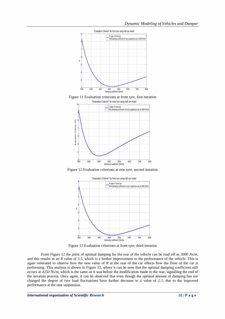
The motion at the rear unsprung mass is dependent upon the motion at the front unsprung mass, and

vice versa. So the next step is to continue this as an iterative process by setting the front damping coefficient to

the new determined optimal value of 4250 Ns/m, and repeating the process for the rear tyre load fluctuations, as is done in Figure 12. The first thing to note is that in Figure 10, the optimal damping coefficient for the rear is

found to be 3250 Ns/m that resulted in R value of 3.9 at the rear tyre. In Figure 12, the damping coefficient at

the front of the vehicle has been further optimised, and this changed the optimal point of damping for the rear.

Even so, if the rear was to be left at the value of 3250 Ns/m, the new value of R is 3.55. In other words, by

improving the performance of the front of the car, the performance at the rear of the car has also improved, even

without making any changes to the settings at the rear. This happens because the displacement fluctuations at

the front of the vehicle transmit through the suspension, into the sprung mass of the vehicle, and ultimately to

the rear tyre. So by reducing the tyre load fluctuations at the front, the tyre load fluctuations at the rear are also

reduced.



1000 2000 3000 4000 5000 6000 7000 80002

3

4

5

6

7

8

9


R

"Evaluation Criterion" for front tyre using half car model

R value of front tyre With damping coefficient of rear suspension set at 3250 N/m/s

Figure 11 Evaluation criterions at front tyre, first iteration

1000 2000 3000 4000 5000 6000 7000 80003

4

5

6

7

8

9

10


Evalu

ation C

riterio

n (

R)

"Evaluation Criterion" for reae tyre using half car model

R value of rear tyre With damping coefficient of front suspension set at 4250 N/m/s

Figure 12 Evaluation criterions at rear tyre, second iteration

1000 2000 3000 4000 5000 6000 7000 80002

3

4

5

6

7

8

9


R

"Evaluation Criterion" for front tyre using half car model

R value of front tyre With damping coefficient of rear suspension set at 3000 N/m/s

Figure 13 Evaluation criterions at front tyre, third iteration

From Figure 12 the point of optimal damping for the rear of the vehicle can be read off as 3000 Ns/m,

and this results in an R value of 3.5, which is a further improvement to the performance of the vehicle. This is

again reiterated to observe how the new value of R at the rear of the car effects how the front of the car is

performing. This analysis is shown in Figure 13, where it can be seen that the optimal damping coefficient still

occurs at 4250 Ns/m, which is the same as it was before the modification made to the rear, signalling the end of

the iteration process. Once again, it can be observed that even though the optimal amount of damping has not

changed the degree of tyre load fluctuations have further decrease to a value of 2.1, due to the improved

performance at the rear suspension.



REFRENCES [1] Zhang, Z., Yu, J., "Design Process of a Double Wish-Bone Suspension"Proceedings of the 2008 SAE

Interntional Powertrains, Fuels and Lubricants

[2] 2008, Supercars, "Supercar Operations Manual", The Official Website of Supercars Australia. [Online] [Cited: 10th October 2008] http://www.v8supercars.com.au/content/tech/v8_

supercar_operations_manual/.

[3] Dixon, J.C., The Shock Absorber Handbook, John Wiley and Sons, West Sussex 2007.

[4] Karnopp, D., "Active and Semi-Active Vibration Isolation", Journal of Mechanical Design, 117, 177-

185 (1995)

[5] Nowlan, D., "Finding the Sweet Spot", International Journal of Motorsport Engineering, 18(2), 52-58

(2008).

[6] Elmadany, M. M., and Abduljabbar, Z. S.,1999, “Linear Quadratic Gaussian Control of a Half-Car

Suspension”. Vehicle System Dynamics Vol. 32, Issue 6, pp. 479-497.

[7] Giua, A., Seatzu, C., and Usai, G., 2000, “A Mixed Suspension System for a Half-Car Vehicle Model”,

Dynamics and Control 10, 375 -397. [8] Andrén, P., 2006, "Power Spectral Density Approximation of Longitudinal Road Profile", International

Journal of Vehicle Design 40, 2-14.

[9] Tamboli, J. A, and Joshi, S.G.,January 1999, “Optimum Design of a Passive Suspension System of a

Vehicle Subjected to Actual Random Road Excitations”, Journal of Sound and Vibration, Volume 219,

Number 2, pp. 193-205(13).

[10] Takahashi, T., 2003, “Modelling, analysis and control methods for improving vehicle dynamic

behaviour” (Overview), R&D Review of Toyota CRDL 38, pp. 1–9.

http://www.v8supercars.com.au/content/tech/v8_%20supercar_operations_manual/

