Incorporating some sustainability issues in lot-sizing models

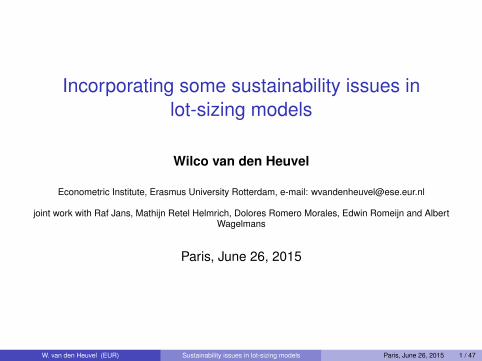
Incorporating some sustainability issues inlot-sizing models

Wilco van den Heuvel

Econometric Institute, Erasmus University Rotterdam, e-mail: [email protected]

joint work with Raf Jans, Mathijn Retel Helmrich, Dolores Romero Morales, Edwin Romeijn and AlbertWagelmans

Paris, June 26, 2015

W. van den Heuvel (EUR) Sustainability issues in lot-sizing models Paris, June 26, 2015 1 / 47

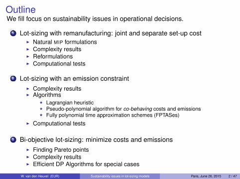
OutlineWe fill focus on sustainability issues in operational decisions.

1 Lot-sizing with remanufacturing: joint and separate set-up costI Natural MIP formulationsI Complexity resultsI ReformulationsI Computational tests

2 Lot-sizing with an emission constraintI Complexity resultsI Algorithms

F Lagrangian heuristicF Pseudo-polynomial algorithm for co-behaving costs and emissionsF Fully polynomial time approximation schemes (FPTASes)

I Computational tests

3 Bi-objective lot-sizing: minimize costs and emissionsI Finding Pareto pointsI Complexity resultsI Efficient DP Algorithms for special cases


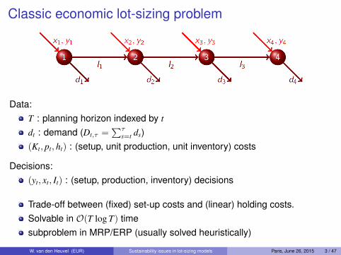
Classic economic lot-sizing problem

Data:T : planning horizon indexed by t

dt : demand (Dt,τ =∑τ

s=t ds)(Kt, pt, ht) : (setup, unit production, unit inventory) costs

Decisions:(yt, xt, It) : (setup, production, inventory) decisions

Trade-off between (fixed) set-up costs and (linear) holding costs.Solvable in O(T log T) timesubproblem in MRP/ERP (usually solved heuristically)


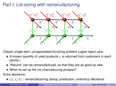
Part I: Lot-sizing with remanufacturing

Classic single-item, uncapacitated lot-sizing problem (upper layer) plus:A known quantity of used products rt is returned from customers in eachperiod t.‘Returns’ can be remanufactured, so that they are as good as new.When to set up the (re-)manufacuring process?

Extra decisions:(yr

t , xrt , I

rt ) : remanufacturing (setup, production, inventory) decisions


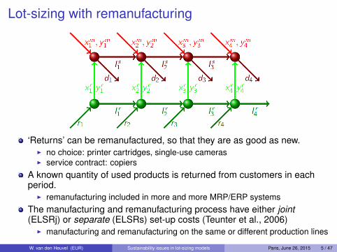
Lot-sizing with remanufacturing

‘Returns’ can be remanufactured, so that they are as good as new.I no choice: printer cartridges, single-use camerasI service contract: copiers

A known quantity of used products is returned from customers in eachperiod.

I remanufacturing included in more and more MRP/ERP systemsThe manufacturing and remanufacturing process have either joint(ELSRj) or separate (ELSRs) set-up costs (Teunter et al., 2006)

I manufacturing and remanufacturing on the same or different production lines


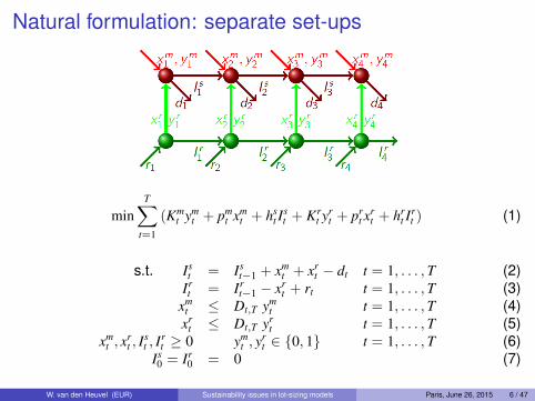
Natural formulation: separate set-ups

minT∑

t=1

(Kmt ym

t + pmt xm

t + hst I

st + Kr

t yrt + pr

t xrt + hr

t Irt ) (1)

s.t. Ist = Is

t−1 + xmt + xr

t − dt t = 1, . . . ,T (2)Irt = Ir

t−1 − xrt + rt t = 1, . . . ,T (3)

xmt ≤ Dt,T ym

t t = 1, . . . ,T (4)xr

t ≤ Dt,T yrt t = 1, . . . ,T (5)

xmt , x

rt , I

st , I

rt ≥ 0 ym

t , yrt ∈ {0, 1} t = 1, . . . ,T (6)

Is0 = Ir

0 = 0 (7)


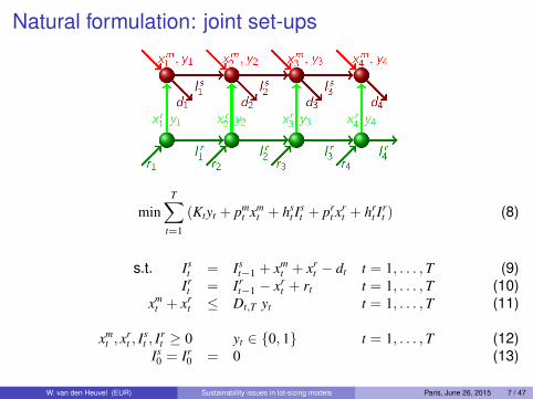
Natural formulation: joint set-ups

minT∑

t=1

(Ktyt + pmt xm

t + hst I

st + pr

t xrt + hr

t Irt ) (8)

s.t. Ist = Is

t−1 + xmt + xr

t − dt t = 1, . . . ,T (9)Irt = Ir

t−1 − xrt + rt t = 1, . . . ,T (10)

xmt + xr

t ≤ Dt,T yt t = 1, . . . ,T (11)

xmt , x

rt , I

st , I

rt ≥ 0 yt ∈ {0, 1} t = 1, . . . ,T (12)

Is0 = Ir

0 = 0 (13)


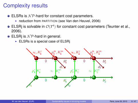
Complexity results

ELSRs is NP-hard for constant cost parameters.I reduction from PARTITION (see Van den Heuvel, 2006)

ELSRj is solvable in O(T4) for constant cost parameters (Teunter et al.,2006).ELSRj is NP-hard in general.

I ELSRs is a special case of ELSRj


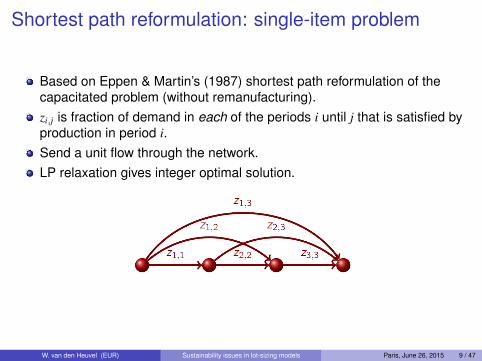
Shortest path reformulation: single-item problem

Based on Eppen & Martin’s (1987) shortest path reformulation of thecapacitated problem (without remanufacturing).zi,j is fraction of demand in each of the periods i until j that is satisfied byproduction in period i.Send a unit flow through the network.LP relaxation gives integer optimal solution.


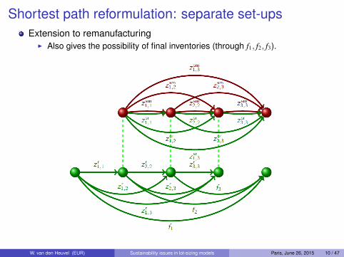
Shortest path reformulation: separate set-upsExtension to remanufacturing

I Also gives the possibility of final inventories (through f1, f2, f3).


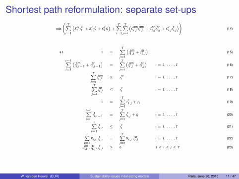
Shortest path reformulation: separate set-ups

min

T∑t=1

(Km

t ymt + Kr

t yrt + Cf

t ft)

+

T∑i=1

T∑j=i

(Csm

i,j zsmi,j + Csr

i,jzsri,j + Cr

i,jzri,j

) (14)

s.t. 1 =

T∑j=1

(zsm1,j + zsr

1,j

)(15)

t−1∑i=1

(zsmi,t−1 + zsr

i,t−1)

=T∑

j=t

(zsmt,j + zsr

t,j

)t = 2, . . . , T (16)

T∑j=t

zsmt,j ≤ ym

t t = 1, . . . , T (17)

T∑j=t

zsrt,j ≤ yr

t t = 1, . . . , T (18)

1 =T∑

j=1zr1,j + f1 (19)

t−1∑i=1

zri,t−1 =T∑

j=tzrt,j + ft t = 2, . . . , T (20)

t∑i=1

zri,t ≤ yrt t = 1, . . . , T (21)

t∑i=1

Ri,t zri,t =T∑

j=tDt,j zsr

t,j t = 1, . . . , T (22)

zsmi,j , zsr

i,j, zri,j ≥ 0 1 ≤ i ≤ j ≤ T (23)


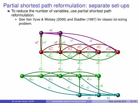
Partial shortest path reformulation: separate set-upsTo reduce the number of variables, use partial shortest pathreformulation.

I See Van Vyve & Wolsey (2006) and Stadtler (1997) for classic lot-sizingproblem.


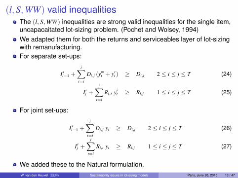
(l, S,WW) valid inequalitiesThe (l, S,WW) inequalities are strong valid inequalities for the single item,uncapacaitated lot-sizing problem. (Pochet and Wolsey, 1994)We adapted them for both the returns and serviceables layer of lot-sizingwith remanufacturing.For separate set-ups:

Isi−1 +

j∑t=i

Dt,j (ymt + yr

t ) ≥ Di,j 2 ≤ i ≤ j ≤ T (24)

Irj +

j∑t=i

Ri,t yrt ≥ Ri,j 1 ≤ i ≤ j ≤ T (25)

For joint set-ups:

Isi−1 +

j∑t=i

Dt,j yt ≥ Di,j 2 ≤ i ≤ j ≤ T (26)

Irj +

j∑t=i

Ri,t yt ≥ Ri,j 1 ≤ i ≤ j ≤ T (27)

We added these to the Natural formulation.W. van den Heuvel (EUR) Sustainability issues in lot-sizing models Paris, June 26, 2015 13 / 47

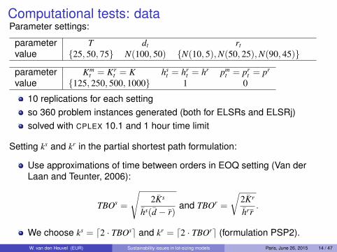
Computational tests: dataParameter settings:

parameter T dt rt

value {25, 50, 75} N(100, 50) {N(10, 5),N(50, 25),N(90, 45)}

parameter Kmt = Kr

t = K hst = hr

t = hr pmt = pr

t = pr

value {125, 250, 500, 1000} 1 0

10 replications for each settingso 360 problem instances generated (both for ELSRs and ELSRj)solved with CPLEX 10.1 and 1 hour time limit

Setting ks and kr in the partial shortest path formulation:

Use approximations of time between orders in EOQ setting (Van derLaan and Teunter, 2006):

TBOs =

√2Ks

hs(d − r)and TBOr =

√2Kr

hr r.

We choose ks = d2 · TBOse and kr = d2 · TBOre (formulation PSP2).W. van den Heuvel (EUR) Sustainability issues in lot-sizing models Paris, June 26, 2015 14 / 47

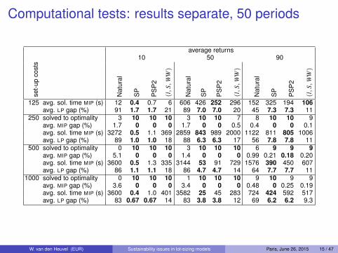
Computational tests: results separate, 50 periods

average returns10 50 90

set-u

pco

sts

Nat

ural

SP

PS

P2

(l,

S,W

W)

Nat

ural

SP

PS

P2

(l,

S,W

W)

Nat

ural

SP

PS

P2

(l,

S,W

W)

125 avg. sol. time MIP (s) 12 0.4 0.7 6 606 426 252 296 152 325 194 106avg. LP gap (%) 91 1.7 1.7 21 89 7.0 7.0 20 45 7.3 7.3 11

250 solved to optimality 3 10 10 10 3 10 10 7 8 10 10 9avg. MIP gap (%) 1.7 0 0 0 1.7 0 0 0.5 0.4 0 0 0.1avg. sol. time MIP (s) 3272 0.5 1.1 369 2859 843 989 2000 1122 811 805 1006avg. LP gap (%) 89 1.0 1.0 18 88 6.3 6.3 17 56 7.8 7.8 11

500 solved to optimality 0 10 10 10 3 10 10 10 6 9 9 9avg. MIP gap (%) 5.1 0 0 0 1.4 0 0 0 0.99 0.21 0.18 0.20avg. sol. time MIP (s) 3600 0.5 1.3 335 3144 53 91 729 1576 390 450 607avg. LP gap (%) 86 1.1 1.1 18 86 4.7 4.7 14 64 7.7 7.7 11

1000 solved to optimality 0 10 10 10 1 10 10 10 9 10 9 9avg. MIP gap (%) 3.6 0 0 0 3.4 0 0 0 0.48 0 0.25 0.19avg. sol. time MIP (s) 3600 0.4 1.0 401 3582 25 45 283 724 424 592 517avg. LP gap (%) 83 0.67 0.67 14 83 3.8 3.8 12 69 6.2 6.2 9.3


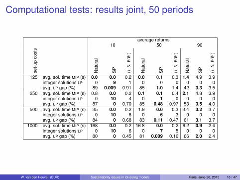
Computational tests: results joint, 50 periods

average returns10 50 90

set-u

pco

sts

Nat

ural

SP

(l,

S,W

W)

Nat

ural

SP

(l,

S,W

W)

Nat

ural

SP

(l,

S,W

W)

125 avg. sol. time MIP (s) 0.0 0.0 0.2 0.0 0.1 0.3 1.4 4.9 3.9integer solutions LP 0 9 1 0 0 0 0 0 0avg. LP gap (%) 89 0.009 0.91 85 1.0 1.4 42 3.3 3.5

250 avg. sol. time MIP (s) 0.8 0.0 0.2 0.1 0.1 0.4 2.1 4.8 3.9integer solutions LP 0 10 4 0 1 0 0 0 0avg. LP gap (%) 87 0 0.70 85 0.48 0.97 53 3.5 4.0

500 avg. sol. time MIP (s) 35 0.0 0.2 1.9 0.0 0.3 3.4 3.2 3.7integer solutions LP 0 10 6 0 6 3 0 0 0avg. LP gap (%) 84 0 0.68 83 0.11 0.47 61 3.1 3.7

1000 avg. sol. time MIP (s) 168 0.0 0.2 16.8 0.0 0.2 6.2 0.9 2.4integer solutions LP 0 10 6 0 7 5 0 0 0avg. LP gap (%) 80 0 0.45 81 0.009 0.16 66 2.0 2.4


Part II: Lot-sizing with an emission constraint

Quantitative models for carbon footprint in SCM:

Emissions and the design of the supply chaine.g. (Cachon, 2011)Emissions and the choice of transportation modee.g. (Hoen et al., 2014)Emissions and the level of data aggregatione.g. (Velázquez-Martínez et al., 2014)Emissions and the management of inventorye.g. (Hua et al., 2011)Emissions and operational decisionse.g. (Benjaafar et al., 2013)


Lot-sizing with an emission constraint

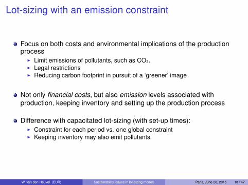
Focus on both costs and environmental implications of the productionprocess

I Limit emissions of pollutants, such as CO2.I Legal restrictionsI Reducing carbon footprint in pursuit of a ‘greener’ image

Not only financial costs, but also emission levels associated withproduction, keeping inventory and setting up the production process

Difference with capacitated lot-sizing (with set-up times):I Constraint for each period vs. one global constraintI Keeping inventory may also emit pollutants.


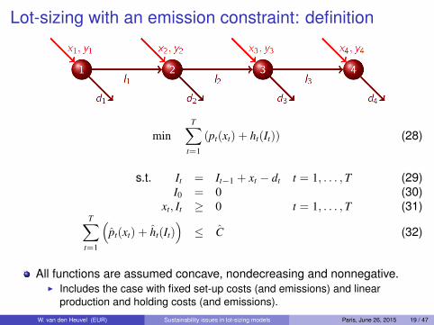
Lot-sizing with an emission constraint: definition

minT∑

t=1

(pt(xt) + ht(It)) (28)

s.t. It = It−1 + xt − dt t = 1, . . . ,T (29)I0 = 0 (30)

xt, It ≥ 0 t = 1, . . . ,T (31)T∑

t=1

(pt(xt) + ht(It)

)≤ C (32)

All functions are assumed concave, nondecreasing and nonnegative.I Includes the case with fixed set-up costs (and emissions) and linear

production and holding costs (and emissions).W. van den Heuvel (EUR) Sustainability issues in lot-sizing models Paris, June 26, 2015 19 / 47

Some related literature

Benjaafar et al. (2013):I Four emission policies: (i) taxes, (ii) caps, (iii) cap-and-trade mechanisms

and (iv) offsetsI It illustrates the impact of lot-sizing decisions on emissions

Absi et al. (2013):I Unit emission cap of the combination of production modesI Four models: (i) periodic, (ii) cumulative, (iii) global and (iv) rollingI Periodic polynomial, the rest NP-complete


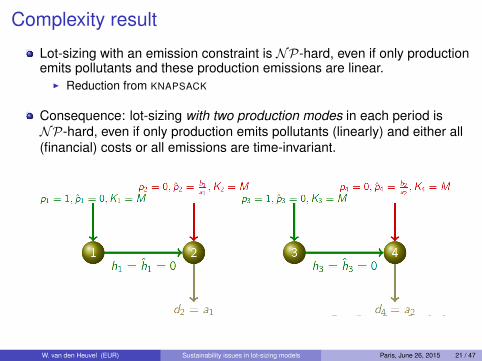
Complexity result

Lot-sizing with an emission constraint is NP-hard, even if only productionemits pollutants and these production emissions are linear.

I Reduction from KNAPSACK

Consequence: lot-sizing with two production modes in each period isNP-hard, even if only production emits pollutants (linearly) and either all(financial) costs or all emissions are time-invariant.


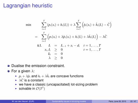
Lagrangian heuristic

minT∑

t=1

(pt(xt) + ht(It)) + λT∑

t=1

(pt(xt) + ht(It)− C

)=

T∑t=1

(pt(xt) + λpt(xt) + ht(It) + λht(It)

)− λC

s.t. It = It−1 + xt − dt t = 1, . . . , Txt, It ≥ 0 t = 1, . . . , T

I0 = 0λ ≥ 0

Dualise the emission constraint.For a given λ:

I pt + λpt and ht + λht are concave functionsI λC is a constantI we have a classic (uncapacitated) lot-sizing problemI solvable in O(T2)


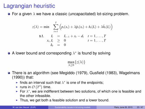
Lagrangian heuristicFor a given λ we have a classic (uncapacitated) lot-sizing problem.

z(λ) = minT∑

t=1

(pt(xt) + λpt(xt) + ht(It) + λht(It)

)s.t. It = It−1 + xt − dt t = 1, . . . , T

xt, It ≥ 0 t = 1, . . . , TI0 = 0

A lower bound and corresponding λ∗ is found by solving

maxλ≥0{z(λ)}

There is an algorithm (see Megiddo (1979), Gusfield (1983), Wagelmans(1990)) that:

I finds an interval such that λ∗ is one of the endpoints;I runs in O

(T4) time.

I For λ∗, we are indifferent between two solutions, of which one is feasible andthe other infeasible.

I Thus, we get both a feasible solution and a lower bound.


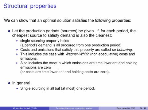
Structural properties

We can show that an optimal solution satisfies the following properties:

Let the production periods (sources) be given. If, for each period, thecheapest source to satisfy demand is also the cleanest:

I single sourcing property holds(a period’s demand is all procured from one production period)

I Costs and emissions that satisfy this property are called co-behaving.I This includes the case with Wagner-Whitin (non-speculative) costs and

emissions.I Also includes the case in which emissions are time-invariant and holding

emissions are zero(or costs are time-invariant and holding costs are zero).

In general:I Single sourcing in all but (at most) one period.


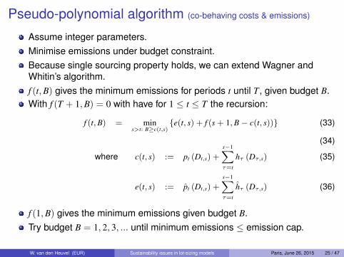
Pseudo-polynomial algorithm (co-behaving costs & emissions)

Assume integer parameters.Minimise emissions under budget constraint.Because single sourcing property holds, we can extend Wagner andWhitin’s algorithm.f (t,B) gives the minimum emissions for periods t until T, given budget B.With f (T + 1,B) = 0 with have for 1 ≤ t ≤ T the recursion:

f (t,B) = mins>t: B≥c(t,s)

{e(t, s) + f (s + 1,B− c(t, s))} (33)

(34)

where c(t, s) := pt (Dt,s) +

s−1∑τ=t

hτ (Dτ,s) (35)

e(t, s) := pt (Dt,s) +

s−1∑τ=t

hτ (Dτ,s) (36)

f (1,B) gives the minimum emissions given budget B.Try budget B = 1, 2, 3, ... until minimum emissions ≤ emission cap.


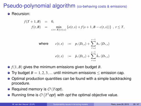
Pseudo-polynomial algorithm (co-behaving costs & emissions)

Recursion:

f (T + 1,B) = 0,


{e(t, s) + f (s + 1,B− c(t, s))} , t ≤ T,

where c(t, s) := pt (Dt,s) +

s−1∑τ=t

hτ (Dτ,s)

e(t, s) := pt (Dt,s) +

s−1∑τ=t

hτ (Dτ,s)

f (1,B) gives the minimum emissions given budget B.Try budget B = 1, 2, 3, ... until minimum emissions ≤ emission cap.Optimal production quantities can be found with a simple backtrackingprocedure.Required memory is O (Topt).Running time is O

(T2opt

)with opt the optimal objective value.


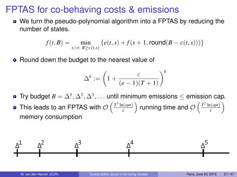
FPTAS for co-behaving costs & emissionsWe turn the pseudo-polynomial algorithm into a FPTAS by reducing thenumber of states.


{e(t, s) + f (s + 1, round(B− c(t, s)))}

Round down the budget to the nearest value of

∆k :=

(1 +

ε

(e− 1)(T + 1)

)k

Try budget B = ∆1,∆2,∆3, . . . until minimum emissions ≤ emission cap.

This leads to an FPTAS with O(

T3 ln(opt)ε

)running time and O

(T2 ln(opt)

ε

)memory consumption


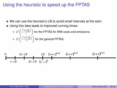
Using the heuristic to speed up the FPTAS

We can use the heuristic’s LB to avoid small intervals at the start.Using this idea leads to improved running times:

I O(

T3 ln( optLB )

ε

)for the FPTAS for WW costs and emissions;

I O(

T4 ln2( optLB )

ε2

)for the general FPTAS.


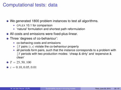
Computational tests: data

We generated 1800 problem instances to test all algorithms.I CPLEX 10.1 for comparisonI ‘natural’ formulation and shortest path reformulation

All costs and emissions were fixed-plus-linear.Three ‘degrees of co-behaviour’:

I co-behaving costs and emissionsI 1

2 T pairs (t, s) violate the co-behaviour propertyI all periods form pairs, such that the instance corresponds to a problem with

12 T periods with two production modes: ‘cheap & dirty’ and ‘expensive &clean’

T = 25, 50, 100ε = 0.10, 0.05, 0.01


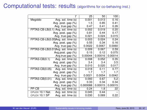
Computational tests: results (algorithms for co-behaving inst.)

T 25 50 100Megiddo Avg. sol. time (s) 0.001 0.013 0.16

Avg. post. gap (%) 1.5 0.85 0.41Avg. true gap (%) 0.47 0.41 0.26

FPTAS-CB-LB(0.1) Avg. sol. time (s) 0.002 0.019 0.20Avg. post. gap (%) 0.81 0.44 0.17Avg. true gap (%) 0.021 0.024 0.015

FPTAS-CB-LB(0.05)Avg. sol. time (s) 0.003 0.024 0.24Avg. post. gap (%) 0.55 0.34 0.16Avg. true gap (%) 0.0022 0.0067 0.0060

FPTAS-CB-LB(0.01)Avg. sol. time (s) 0.009 0.067 0.59Avg.post. gap (%) 0.15 0.12 0.075Avg.true gap (%) 0.00044 0.00016 0.00014

FPTAS-CB(0.1) Avg. sol. time (s) 0.008 0.052 0.35Avg. post. gap (%) 3.4 3.4 3.5Avg. true gap (%) 0.010 0.020 0.017



PP-CB Avg. sol. time (s) 0.24 1.8 22CPLEX 10.1 Nat. Avg. sol. time (s) 0.045 0.44 –CPLEX 10.1 SP Avg. sol. time (s) 0.030 0.069 0.22


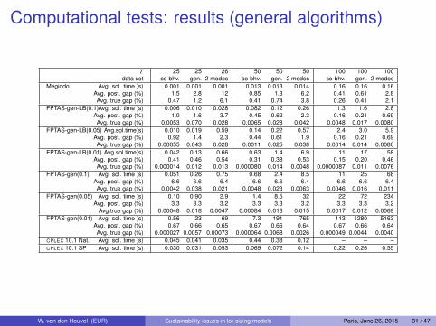
Computational tests: results (general algorithms)

T 25 25 26 50 50 50 100 100 100data set co-bhv. gen. 2 modes co-bhv. gen. 2 modes co-bhv. gen. 2 modes

Megiddo Avg. sol. time (s) 0.001 0.001 0.001 0.013 0.013 0.014 0.16 0.16 0.16Avg. post. gap (%) 1.5 2.8 12 0.85 1.3 6.2 0.41 0.61 2.8Avg. true gap (%) 0.47 1.2 6.1 0.41 0.74 3.8 0.26 0.41 2.1

FPTAS-gen-LB(0.1)Avg. sol. time (s) 0.006 0.010 0.028 0.082 0.12 0.26 1.3 1.6 2.8Avg. post. gap (%) 1.0 1.6 3.7 0.45 0.62 2.3 0.16 0.21 0.69Avg. true gap (%) 0.0053 0.070 0.028 0.0065 0.028 0.042 0.0048 0.017 0.0080

FPTAS-gen-LB(0.05) Avg.sol.time(s) 0.010 0.019 0.59 0.14 0.22 0.57 2.4 3.0 5.9Avg. post. gap (%) 0.92 1.4 2.3 0.44 0.61 1.9 0.16 0.21 0.69Avg. true gap (%) 0.00055 0.043 0.028 0.0011 0.025 0.038 0.0014 0.014 0.0080

FPTAS-gen-LB(0.01) Avg.sol.time(s) 0.042 0.13 0.66 0.63 1.4 6.9 11 17 58Avg. post. gap (%) 0.41 0.46 0.54 0.31 0.38 0.53 0.15 0.20 0.46Avg. true gap (%) 0.000014 0.012 0.013 0.000080 0.014 0.0048 0.0000087 0.011 0.0076

FPTAS-gen(0.1) Avg. sol. time (s) 0.051 0.26 0.75 0.68 2.4 8.5 11 25 68Avg. post. gap (%) 6.6 6.6 6.4 6.6 6.6 6.4 6.6 6.6 6.4Avg. true gap (%) 0.0042 0.038 0.021 0.0048 0.023 0.0063 0.0046 0.016 0.011

FPTAS-gen(0.05) Avg. sol. time (s) 0.10 0.90 2.9 1.4 8.5 32 22 72 234Avg. post. gap (%) 3.3 3.3 3.2 3.3 3.3 3.2 3.3 3.3 3.2

Avg.true gap (%) 0.00048 0.018 0.0047 0.00084 0.018 0.015 0.0017 0.012 0.0069FPTAS-gen(0.01) Avg. sol. time (s) 0.56 23 69 7.3 191 765 113 1280 5163

Avg. post. gap (%) 0.67 0.66 0.65 0.67 0.66 0.64 0.67 0.66 0.64Avg. true gap (%) 0.000027 0.0057 0.00073 0.000064 0.0068 0.0026 0.000049 0.0044 0.0040

CPLEX 10.1 Nat. Avg. sol. time (s) 0.045 0.041 0.035 0.44 0.38 0.12 – – –CPLEX 10.1 SP Avg. sol. time (s) 0.030 0.031 0.053 0.069 0.072 0.14 0.22 0.26 0.55


Part III: Bi-Objective Lot-Sizing Problems

Data:T : planning horizon indexed by t

dt : demand (dt,τ =∑τ

s=t ds)(ft, ct, ht) : (setup, unit production, unit inventory) costs(ft, ct, ht) : (setup, unit production, unit inventory) emissions` : length of the emission block

Decisions:(yt, xt, It) : (setup, production, inventory) decisions


Different levels of aggregation for emissions

Partitioning the planning horizon:

We partition the planning horizon into blocks of length `We minimize the max emission over the blocks (T/` blocks in total)Different levels of aggregation depending on `

Special cases:

Whole-horizon emissions (` = T)Period emissions (` = 1)


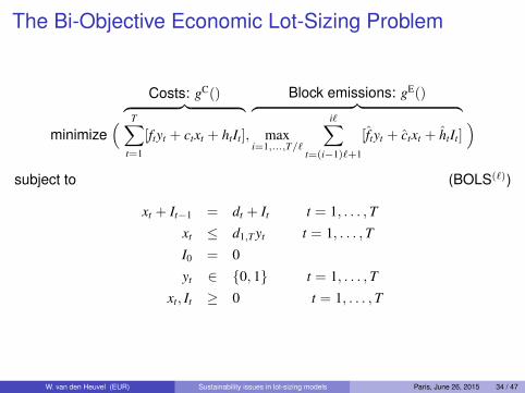
The Bi-Objective Economic Lot-Sizing Problem

minimize( Costs: gC()︷︸︸︷

T∑t=1

[ftyt + ctxt + htIt],

Block emissions: gE()︷︸︸︷max

i=1,...,T/`

i∑t=(i−1)`+1

[ftyt + ctxt + htIt])

subject to (BOLS(`))

xt + It−1 = dt + It t = 1, . . . ,Txt ≤ d1,Tyt t = 1, . . . ,TI0 = 0yt ∈ {0, 1} t = 1, . . . ,T

xt, It ≥ 0 t = 1, . . . ,T


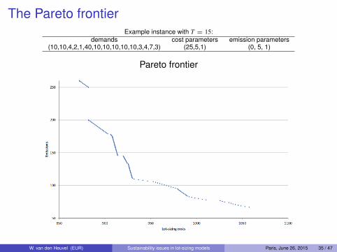
The Pareto frontierExample instance with T = 15:

demands cost parameters emission parameters(10,10,4,2,1,40,10,10,10,10,10,3,4,7,3) (25,5,1) (0, 5, 1)

Pareto frontier


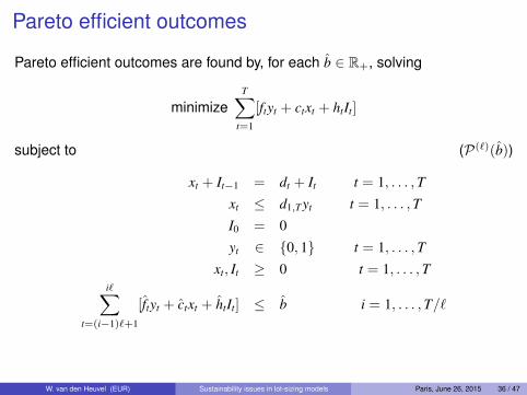
Pareto efficient outcomes

Pareto efficient outcomes are found by, for each b ∈ R+, solving

minimizeT∑

t=1

[ftyt + ctxt + htIt]

subject to (P(`)(b))


xt, It ≥ 0 t = 1, . . . ,Ti∑

t=(i−1)`+1

[ftyt + ctxt + htIt] ≤ b i = 1, . . . ,T/`


ε-dominating sets

Difficulty of multi-objective problems:Describing the Pareto frontier is challenging in Multi-ObjectiveCombinatorial Optimization Ulungu and Teghem (1994); Ehrgott andGandibleux (2000, 2004)Focus on ε-dominating set in the outcome space, see e.g. Blanquero andCarrizosa (2002)

Definition: Z∗ is an ε-dominating set for

minz∈Z

(gC(z), gE(z))

if, for each z ∈ Z, there exists a z∗ ∈ Z∗ such that

gC(z∗) ≤ gC(z) + ε andgE(z∗) ≤ gE(z) + ε


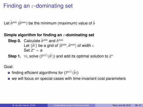
Finding an ε-dominating set

Let bmin (bmax) be the minimum (maximum) value of b

Simple algorithm for finding an ε-dominating setStep 0. Calculate bmin and bmax

Let {bi} be a grid of [bmin, bmax] of width εSet Z∗ = ø

Step 1. ∀i, solve (P(`)(bi)) and add its optimal solution to Z∗

Goal:finding efficient algorithms for (P(`)(b))we will focus on special cases with time-invariant cost parameters


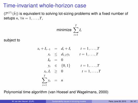
Time-invariant whole-horizon case(P(T)(b)) is equivalent to solving lot-sizing problems with a fixed number ofsetups n, ∀n = 1, . . . ,T,

minimizeT∑

t=1

It

subject to


xt, It ≥ 0 t = 1, . . . ,TT∑

t=1

yt = n

Polynomial time algorithm (van Hoesel and Wagelmans, 2000)


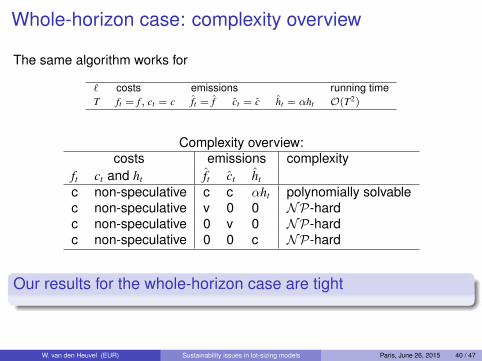
Whole-horizon case: complexity overview

The same algorithm works for

` costs emissions running timeT ft = f , ct = c ft = f ct = c ht = αht O(T2)

Complexity overview:costs emissions complexity

ft ct and ht ft ct ht

c non-speculative c c αht polynomially solvablec non-speculative v 0 0 NP-hardc non-speculative 0 v 0 NP-hardc non-speculative 0 0 c NP-hard

Our results for the whole-horizon case are tight


Time-invariant period caseMain approach:

decomposition the problem in subplans [u, v]

compute the cost of a subplan efficiently

Definitions:A block/period is called tight if its emission constraint is bindingA block/period is called extreme if either tight or no production

Properties:The only possible non-tight production period is u

Consider t (u < t ≤ v) with inventory It such that:I xt := (b− f − hIt)/c > 0,I It−1 := It − xt + dt > 0.

Then t is a tight production period with production quantity xt, andincoming inventory equal to It−1.

Main resultThe optimal cost of all subplans can be calculated in O(T2) time by abackward DP algorithm.


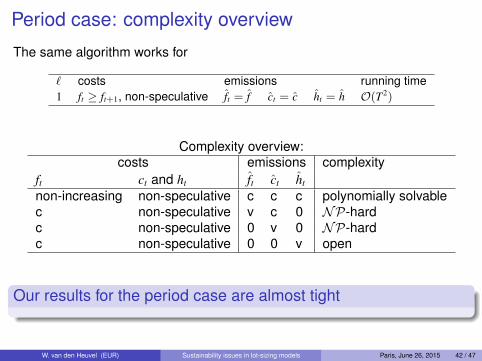
Period case: complexity overview

The same algorithm works for

` costs emissions running time1 ft ≥ ft+1, non-speculative ft = f ct = c ht = h O(T2)

Complexity overview:costs emissions complexity


non-increasing non-speculative c c c polynomially solvablec non-speculative v c 0 NP-hardc non-speculative 0 v 0 NP-hardc non-speculative 0 0 v open

Our results for the period case are almost tight


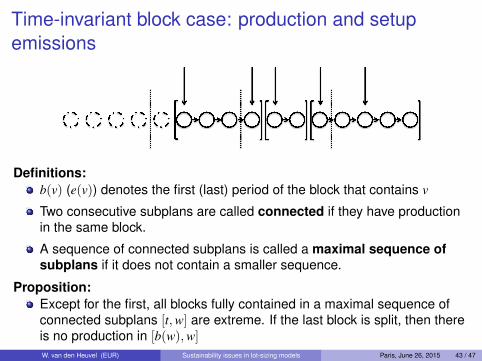
Time-invariant block case: production and setupemissions

Definitions:b(v) (e(v)) denotes the first (last) period of the block that contains v

Two consecutive subplans are called connected if they have productionin the same block.

A sequence of connected subplans is called a maximal sequence ofsubplans if it does not contain a smaller sequence.

Proposition:Except for the first, all blocks fully contained in a maximal sequence ofconnected subplans [t,w] are extreme. If the last block is split, then thereis no production in [b(w),w]


Block case: production and setup emissions

General solution approach:Decompose solution into maximal sequences of connected subplansDecompose maximal sequences in subplansCompute the cost of a subplan efficiently

Main result:We can derive a DP algorithm to compute the subplan costs using:

I (u, v; w), a subplan [u, v] contained in a maximal sequence ending in period wI keeping track of the number of production blocks and setups.

The optimal cost of all subplans can be calculated in O(T7/`) time by abackward DP algorithm.


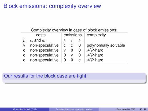
Block emissions: complexity overview

Complexity overview in case of block emissions:costs emissions complexity


v non-speculative c c 0 polynomially solvablec non-speculative v 0 0 NP-hardc non-speculative 0 v 0 NP-hardc non-speculative 0 0 c NP-hard

Our results for the block case are tight


Conclusions & further research1 Lot-sizing with remanufacturing:

I ELSRs and ELSRj are both NP-hard.I Computational tests indicate that reformulations SP and PSP perform well

I Extend shortest path formulations with capacitiesI Use solution of LP relaxation in a rounding heuristicI How to incorporate stochastic returns?

2 Lot-sizing with emission constraint:I is NP-hardI A Lagrangean heuristic gives a LB as well as a feasible solution in O

(T4).

I There is an FPTAS which works faster in case of co-behaviour property.

I applying the same technique to create FPTASes for other problems

3 Bi-objective lot-sizing:I Special classes of problem instances are polynomially solvableI We have shown the tightness of our polynomiality resultsI Results can be used to find an ε-dominating set

I Close the complexity gapI Overlapping blocks caseI Algorithms for the NP-complete cases


References

N. Absi, S. Dauzère-Pérès, S. Kedad-Sidhoum, B. Penz, and C. Rapine. Lot-sizing with carbon emission constraints. European Journal of OperationalResearch, 227(1):55–61, 2013.

S. Benjaafar, Y. Li, and M. Daskin. Carbon footprint and the management of supply chains: Insights from simple models. IEEE Transactions on AutomationScience and Engineering, 10(1):99–116, 2013.

R. Blanquero and E. Carrizosa. A D.C. biobjective location model. Journal of Global Optimization, 23:139–154, 2002.

G.P. Cachon. Supply chain design and the cost of greenhouse gas emissions. Technical report, The Wharton School, University of Pennsylvania, 2011.

M. Ehrgott and X. Gandibleux. A survey and annotated bibliography of multiobjective combinatorial optimization. OR Spektrum, 22:425–460, 2000.

M. Ehrgott and X. Gandibleux. Approximative solution methods for multiobjective combinatorial optimization. TOP, 12(1):1–89, 2004.

K.M.R. Hoen, T. Tan, J.C. Fransoo, and G.J. van Houtum. Effect of carbon emission regulations on transport mode selection under stochastic demand.Flexible Services and Manufacturing Journal, 26(1–2):170–195, 2014.

G. Hua, T.C.E. Cheng, and S. Wang. Managing carbon footprints in inventory management. International Journal of Production Economics, 132:178–185,2011.

E.L. Ulungu and J. Teghem. Multi-objective combinatorial optimization problems: a survey. Journal of Multi-Criteria Decision Analysis, 3:83–104, 1994.

C.P.M. van Hoesel and A.P.M. Wagelmans. Parametric analysis of setup cost in the economic lot-sizing model without speculative motives. InternationalJournal of Production Economics, 66:13–22, 2000.

J.C. Velázquez-Martínez, J.C. Fransoo, E.E. Blanco, and J. Mora-Vargas. The impact of carbon footprinting aggregation on realizing emission reductiontargets. Flexible Services and Manufacturing Journal, 26(1–2):196–220, 2014.


Documents

Incorporating some sustainability issues in lot-sizing models