SUPPLY CHAIN FLOW PLANNING METHODS:

A REVIEW OF THE LOT-SIZING LITERATURE

NAFEE RIZK

and

ALAIN MARTEL

January 2001

Working Paper DT-2001-AM-1

Centre de recherche sur les technologies de l’organisation réseau (CENTOR)

Université Laval, QC, Canada, G1K 7P4

2

Summary

The objective of this paper is to present, in a unified body, the most important research

results dealing with material flow planning in a supply chain, and in particular with

deterministic lot-sizing methods. After identifying the most relevant characteristics of

material flow planning problems, we present clears and simple formulations of the

different lot-sizing problems treated in the literature and we discuss their solution

methods. Special attention is given to the multi-facility material flow coordination

problems and a new formulation of the general problem is proposed.

Résumé

L’objectif de ce document est de présenter, d’une manière unifiée, les plus importants

travaux de recherche qui portent sur les problèmes de pilotage des flux de matières dans

les réseaux logistiques et, en particulier, les méthodes de lotissement déterministes. Après

avoir identifié les caractéristiques fondamentales de ces problèmes, nous présentons des

formulations des principaux cas traités dans la littérature et nous discutions les méthodes

de solutions disponibles. Un intérêt spécial est porté aux problèmes de lotissement dans

les réseaux logistiques qui incluent plusieurs installations et une nouvelle formulation du

problème général est proposée.

3

Table of contents

SUMMARY.....................................................................................................................................2

RÉSUMÉ.........................................................................................................................................2

TABLE OF CONTENTS...............................................................................................................3

I. INTRODUCTION ......................................................................................................................5

II. SINGLE FACILITY PROBLEMS..........................................................................................8

1. SINGLE LEVEL PROBLEMS (SLP)..........................................................................................8

1.1. Uncapacitated Single Item Problems .................................................................................9

1.1.1. Static Demand ...................................................................................................................................................10 1.1.2. Dynamic Demand ..............................................................................................................................................11

1.2. Capacitated Single Item Problems ...................................................................................12

1.2.1. Static Demand ...................................................................................................................................................12 1.2.2. Dynamic Demand ..............................................................................................................................................12

1.2.2.1. The Capacitated Lot-sizing Problem (CLSP)................................................................................................12 1.2.2.2. The Continuous Setup Lot-sizing Problem (CSLP) ......................................................................................13 1.2.2.3. The Discrete Lot-Sizing and Scheduling Problem (DLSP) ..........................................................................14

1.3. Uncapacitated Multi-item Problems.................................................................................14

1.3.1. Static Demand ...................................................................................................................................................15 1.3.2 Dynamic Demand ..............................................................................................................................................16

1.4. Capacitated Multi-item Problems ....................................................................................17

1.4.1. Static Demand ...................................................................................................................................................17 1.4.1.1 ELSP analytical approaches ..........................................................................................................................18 1.4.1.2. ELSP heuristic approaches............................................................................................................................19

1.4.2 Dynamic demand...............................................................................................................................................19 1.4.2.1 The Capacitated Lot-Sizing Problem (CLSP) ...............................................................................................19 1.4.2.2 The Continuous Setup Lot-Sizing Problem (CSLP) .....................................................................................21 1.4.2.3. The Discrete Lot-Sizing and Scheduling Problem (DLSP) ..........................................................................22

2. MULTI-LEVEL PROBLEMS ..................................................................................................22

2.1. Uncapacitated single item problems ................................................................................26

2.1.1. Static demand ....................................................................................................................................................26 2.1.2. Dynamic demand...............................................................................................................................................26

4

2.2. Capacitated single item problems ....................................................................................28

2.2.1. Static demand ....................................................................................................................................................29 2.2.2. Dynamic demand...............................................................................................................................................29

2.3. Uncapacitated multi-item problems .................................................................................30

2.3.1. Static demand ....................................................................................................................................................30 2.3.2 Dynamic demand...............................................................................................................................................31

2.4. Capacitated multi-item problems .....................................................................................31

2.4.1. Static demand ....................................................................................................................................................31 2.4.2. Dynamic demand...............................................................................................................................................32

III. MULTI-FACILITY PROBLEMS .......................................................................................33

1. UNCAPACITATED SINGLE ITEM PROBLEMS ..........................................................................34

1.1. Static demand ...................................................................................................................34

1.2. Dynamic demand ..............................................................................................................37

2. CAPACITATED SINGLE ITEM PROBLEMS ..............................................................................37

3. UNCAPACITATED MULTI-ITEM PROBLEMS...........................................................................38

3.1. Static demand ...................................................................................................................38

3.1.1. One-origin One-destination Network........................................................................................................................38 3.1.2. One-origin Multi-destination Network......................................................................................................................39 3.1.3. Multi-origin Multi-destination Network ...................................................................................................................39

3.2. Dynamic demand ..............................................................................................................41

4. CAPACITATED MULTI-ITEM PROBLEMS ...............................................................................41

IV. A GENERAL SUPPLY CHAIN PLANNING MODEL.....................................................43

V. CONCLUSION........................................................................................................................46

REFERENCES .............................................................................................................................48

5

I. Introduction

Strong foreign competition in an increasingly global marketplace has forced firms to turn

their attention towards streamlining operations in order to generate savings from a

slimmer and more reactive Supply Chain. A.T. Kearney, a management consulting firm

(Sengupta and Turnbull [1996]) estimated that supply chain costs represent more than

80% of the cost structure in a typical manufacturing company. For retailers the supply

chain costs represent between 70% and 80% of their total costs. From these numbers we

can deduce that even a slight improvement in the process of managing the supply chain

can be translated into millions of dollars on the bottom line. Before going further, let’s

define the “Supply Chain”.

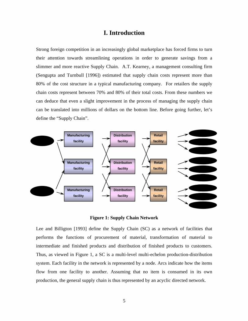
Figure 1: Supply Chain Network

Lee and Billigton [1993] define the Supply Chain (SC) as a network of facilities that

performs the functions of procurement of material, transformation of material to

intermediate and finished products and distribution of finished products to customers.

Thus, as viewed in Figure 1, a SC is a multi-level multi-echelon production-distribution

system. Each facility in the network is represented by a node. Arcs indicate how the items

flow from one facility to another. Assuming that no item is consumed in its own

production, the general supply chain is thus represented by an acyclic directed network.

Distribution

facility

Distribution

facility

Distribution

facility

Supplier

Supplier

Manufacturing

facility

Manufacturing

facility

Manufacturing

facility

Retail

facility

Retail

facility

Retail

facility

Customer

Customer

Customer

Customer

Customer

Customer

Customer

Customer

Customer

6

Once strategic planning has specified the shape and structure of the supply chain, as well

as its production, transportation and storage capacity, the question to answer is how to

plan and control the flow of materials in the network, or how to mange the supply chain?

Supply chain management (SCM), as defined by Sengupta and Turnbull [1996], is the

process of effectively managing the flow of materials and finished goods from vendors to

customers using manufacturing facilities and warehouses as potential intermediate stops.

This problem is one of the most important challenges, especially in a competitive

environment that every enterprise seeks to resolve successfully.

The performance of a SC, as observed by Cohen and Lee [1988], can be measured with

respect to: (1) the cost of the products delivered to markets, (2) the level of service

provided to customers and (3) the responsiveness and flexibility of the

production/distribution system. Managing the supply chain effectively can improve

customer service levels dramatically, reduce excess inventory in the system, and cut

excess costs from the logistic network.

The scientific literature on SCM problems is directly linked to the solution of lot-sizing

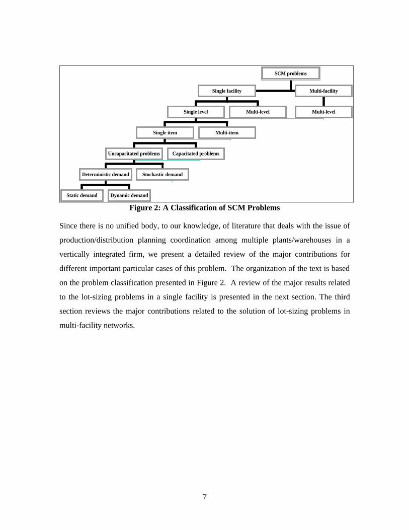
problems in production-distribution networks, and it can be classified into categories

based on the number of locations considered, the number of stages (or echelons) in the

system, the number of items considered, the presence or absence of capacity constraints,

and the characteristics of demand (see Figure 2). Note that the models found in the

literature for each class of problems identified above, may also include different cost

structures and allow for backorders or not.

Since one can deal with the stochastic nature of real manufacturing-distribution networks

through the use of safety buffers, rolling planning horizons and planning time fences

(Graves [1988], Martel et al. [1995], Martel [1995]….); and since most decision systems

are implemented in practice as if the supply chain environment was deterministic over a

specified finite horizon, we restrict our review in this text to deterministic models. Note,

however, that stochastic supply chain models have also attracted the attention of

researchers (see for example, Federgruen [1993] and Axsäter [1993]).

7

Static demand Dynamic demand

Deterministic demand Stochastic demand

Uncapacitated problems Capacitated problems

Single item Multi-item

Single level Multi-level

Single facility

Multi-level

Multi-facility

SCM problems

Figure 2: A Classification of SCM Problems

Since there is no unified body, to our knowledge, of literature that deals with the issue of

production/distribution planning coordination among multiple plants/warehouses in a

vertically integrated firm, we present a detailed review of the major contributions for

different important particular cases of this problem. The organization of the text is based

on the problem classification presented in Figure 2. A review of the major results related

to the lot-sizing problems in a single facility is presented in the next section. The third

section reviews the major contributions related to the solution of lot-sizing problems in

multi-facility networks.

II. Single Facility Problems

Single facility systems are the most studied in the literature. Even if some researchers’

claim that they deal with multi-facility situations, most of them don’t consider

transportation costs and thus the system they consider is often a multi-machine or multi-

stage single facility system. Due to the predominant assumption that the general multi-

facilities problem can be solved by optimizing the costs of each facility independently,

and due to the difficulties of solving such big size problems in real time, the

interdependency between the different facilities in the system are often not considered. In

this section, we review the most important contributions to the solution of single facility

problems in both single stage and multi-stage situations.

1. Single Level Problems (SLP)

Single stage (echelon) systems are common in procurement and distribution contexts.

Even if single stage systems don’t describe truly the real situation of the majority of

production systems, they have attracted the attention of a large proportion of researchers.

This can be explained by the fact that single stage methods may be generalized to deal

effectively with multi-stage situations, they may be used as routines for multi-stage

methods, and they may also give good insights and ideas to deal effectively with more

complex problems.

In single-stage production lot-sizing problems, the manufacturing process is characterized

by a single level product structure in which products are directly produced from raw

materials without intermediate stocking points or subassemblies. Product demands are

derived from customer orders and/or market forecasts. In a procurement/distribution

context, single-echelon lot-sizing problems generally consider only the procurement and

the inventory costs of a single stocking point and do not take transportation costs into

account.

Before going further in our SLP review, we present a generic formulation of the problem.

Using the notation in Figure 3 the SLP can be formulated as follows:

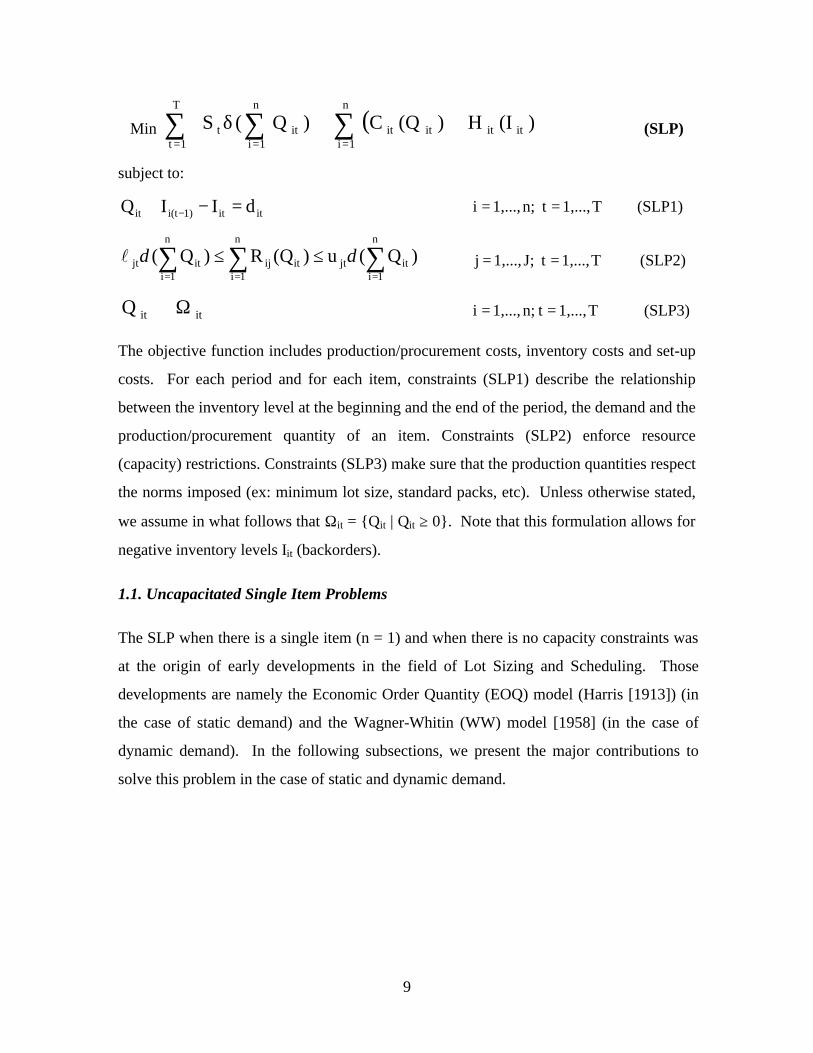
9

Min ( )∑ ∑∑= ==

++δ

T

1t

n

1iitititit

n

1iitt )(IH)(QC)Q(S (SLP)

subject to:

itit1)i(tit dIIQ =−+ − T1,..., tn;1,...,i == (SLP1)

)Q(u)(QR)Q(n

1iitjt

n

1iitij

n

1iitjt ∑∑∑

===

≤≤ δδl T1,..., tJ;1,...,j == (SLP2)

ititQ Ω∈ T1,..., tn;1,...,i == (SLP3)

The objective function includes production/procurement costs, inventory costs and set-up

costs. For each period and for each item, constraints (SLP1) describe the relationship

between the inventory level at the beginning and the end of the period, the demand and the

production/procurement quantity of an item. Constraints (SLP2) enforce resource

(capacity) restrictions. Constraints (SLP3) make sure that the production quantities respect

the norms imposed (ex: minimum lot size, standard packs, etc). Unless otherwise stated,

we assume in what follows that Ωit = Qit | Qit ≥ 0. Note that this formulation allows for

negative inventory levels Iit (backorders).

1.1. Uncapacitated Single Item Problems

The SLP when there is a single item (n = 1) and when there is no capacity constraints was

at the origin of early developments in the field of Lot Sizing and Scheduling. Those

developments are namely the Economic Order Quantity (EOQ) model (Harris [1913]) (in

the case of static demand) and the Wagner-Whitin (WW) model [1958] (in the case of

dynamic demand). In the following subsections, we present the major contributions to

solve this problem in the case of static and dynamic demand.

10

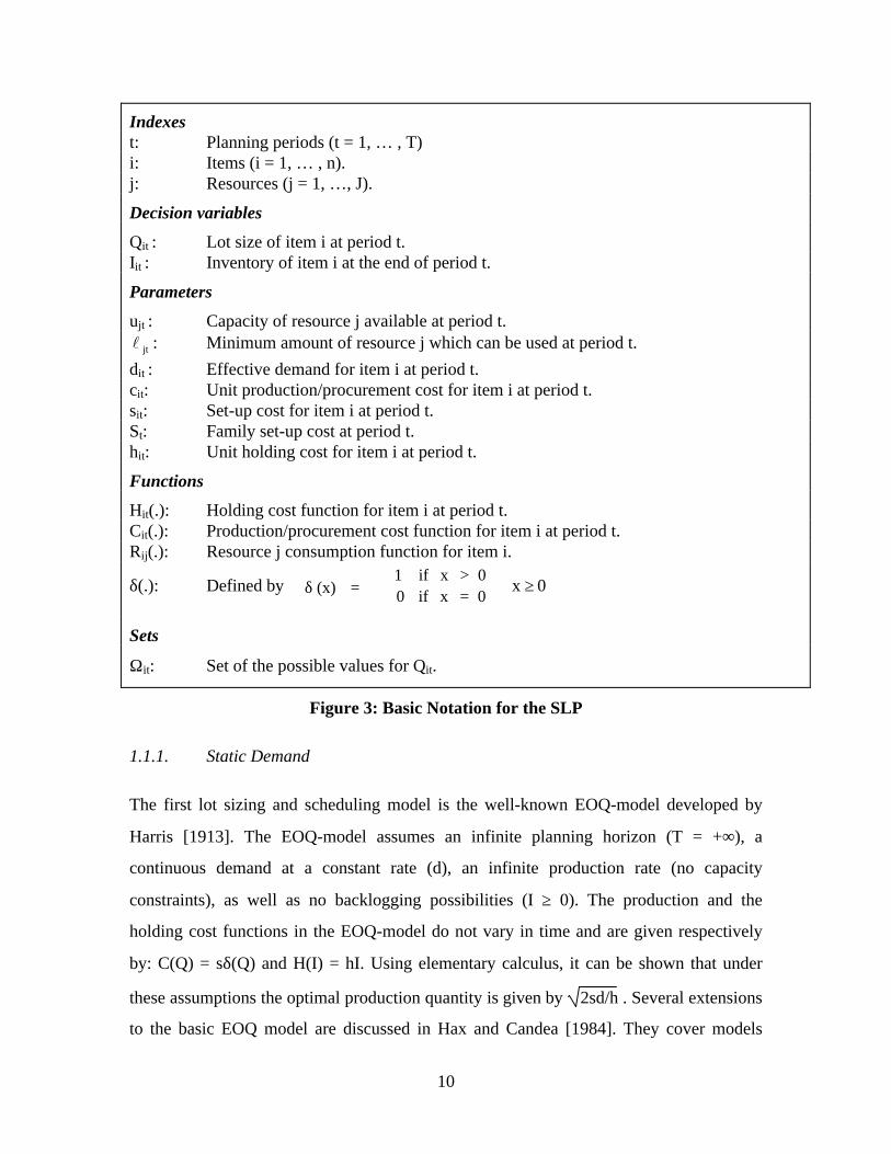
Indexes t: Planning periods (t = 1, … , T) i: Items (i = 1, … , n). j: Resources (j = 1, …, J).

Decision variables

Qit : Lot size of item i at period t. Iit : Inventory of item i at the end of period t.

Parameters

ujt : Capacity of resource j available at period t. jtl : Minimum amount of resource j which can be used at period t.

dit : Effective demand for item i at period t. cit: Unit production/procurement cost for item i at period t. sit: Set-up cost for item i at period t. St: Family set-up cost at period t. hit: Unit holding cost for item i at period t.

Functions

Hit(.): Holding cost function for item i at period t. Cit(.): Production/procurement cost function for item i at period t. Rij(.): Resource j consumption function for item i.

δ(.): Defined by

>

==δ0 x if10 x if 0(x) 0 x ≥∀

Sets

Ωit: Set of the possible values for Qit.

Figure 3: Basic Notation for the SLP

1.1.1. Static Demand

The first lot sizing and scheduling model is the well-known EOQ-model developed by

Harris [1913]. The EOQ-model assumes an infinite planning horizon (T = +∞), a

continuous demand at a constant rate (d), an infinite production rate (no capacity

constraints), as well as no backlogging possibilities (I ≥ 0). The production and the

holding cost functions in the EOQ-model do not vary in time and are given respectively

by: C(Q) = sδ(Q) and H(I) = hI. Using elementary calculus, it can be shown that under

these assumptions the optimal production quantity is given by 2sd/h . Several extensions

to the basic EOQ model are discussed in Hax and Candea [1984]. They cover models

11

which allow for backlogging, lost sales and quantity discounts. Tersine and Price [1981]

discuss the temporary price discounts case. Solutions to finite horizon cases where costs

are time-dependent are presented by Lev and Weiss [1990] and Gascon [1995]. Several

other variants of this basic problem are also found in the literature.

1.1.2. Dynamic Demand

Wagner and Whitin [1958] proposed a dynamic programming algorithm to solve the

problem when demand is time varying, there is no backlogging possibilities, no capacity

constraints, and when the production/procurement and the holding cost functions are

given respectively by Ct(Qt) = stδ(Qt) and Ht(It) = htIt. The WW-model has an O(T2)

running time. In subsequent work, researchers focused on generalizing the WW-procedure

to solve more complicated versions of the original problem. Veinott [1963] showed that

even if production and inventory costs are general concave functions, the problem is still

solvable by an O(T2) dynamic programming algorithm. Zangwill [1966, 1969], Gupta and

Brennan [1992] (among others) generalized the WW-procedure to solve the problem

when backlogging is allowed. Martel and Gascon [1998] proposed an algorithm to solve

the problem when inventory holding cost is a percentage of the product cost. Extensive

research has been done in the case of a perishable, deteriorating or obsolete product. The

main references in this case are Veinott [1960], Van Zyl [1964], Ghare and Schrader

[1963], Shah [1977], Cohen [1977], Tadikamalla [1978], Nahmias and Wang [1979],

Freidman and Hoch [1978] and Jain and Silver [1994]. Since the WW-algorithm is

widely used as a routine in solving more complicated problems, recent work on this

problem focused on bringing down its theoretical running time by exploiting the special

(cost) properties of the problem and by an appropriate choice of data structure (see

Federgruen and Tzur [1991], Wagelmans et al. [1992] and Aggarwal and Park [1993]).

Also, a large number of heuristics have been proposed to solve the WW-model and its

variants. The major contributions are De Matteis and Mendoze [1968] (The Part Period

Balancing heuristic), Gorham [1968] (The Least Unit Cost Heuristic), Berry [1972] (The

EOQ Based Period Order Quantity heuristic), Silver and Meal [1973], Groff [1979],

Zoller and Robrade [1988], Gupta and Brennan [1992], and Jain and Silver [1994].

12

1.2. Capacitated Single Item Problems

The aim of this class of problems is to determine the optimal or near optimal

production plan of a single product while known demands are satisfied and capacity

restrictions are respected.

1.2.1. Static Demand

The basic EOQ model in the case of a finite production rate is discussed in Hax and

Candea [1984], among others.

1.2.2. Dynamic Demand

In the case of dynamic demand the well-known lot-sizing models that deal explicitly with

capacity restrictions are the Capacitated Lot-Sizing Problem (CLSP), the Continuous

Setup Lot-sizing Problem (CSLP) and the Discrete Lot-sizing and Scheduling Problem

(DLSP). In general, these problems ignore setup times. The definition, the complexity

and the solution procedures of the single item version of each of the above mentioned

problems is discussed in what follows.

1.2.2.1. The Capacitated Lot-sizing Problem (CLSP)

The CLSP aims to determine a production/procurement plan that minimizes

production/procurement and inventory holding costs while known demand are satisfied

without backlogging (Iit ≥ 0) and capacity restrictions are respected. In the single level

CLSP, only one resource is considered (J=1) and no lower bound on resource usage is

imposed ( jtl = 0 ∀ j, t). The single item CLSP is shown to be NP-Hard for arbitrary cost

functions or time varying capacity by Florian et al. [1980] and by Bitran and Yanasse

[1982]. Even if it is NP-Hard, the basic problem with production cost, holding cost and

resource consumption functions given respectively by Ct(Qt) = stδ(Qt) + ctQt, Ht(It) = htIt,

and Rt(Qt) = Qt, can be solved by a successful dynamic programming approach proposed

by Chen et al. [1994]. Many authors proposed polynomial algorithms to solve the constant

capacity version of the problem. Florian and Klein [1971] presented an O(T4) dynamic

13

programming algorithm based on the shortest path method to solve the constant capacity

case with concave costs. Their algorithm can deal with the backlogging situation.

Jagannathan and Rao [1973] extended Florian and Klein’s results to a more general

production cost function which is neither concave nor convex. Van Hoesel and

Wagelmans [1996] proposed a more efficient O(T3) dynamic programming algorithm to

solve the constant capacity, concave production costs and linear holding costs case. Hill

[1997] reduced the constant capacity problem where the production/procurement and the

inventory cost are time-invariant and are given respectively by C(Qt) = sδ(Qt) and H(It) =

hIt to a typical WW model that can be solved efficiently. The case with time-dependent

capacity was also treated in the literature. An O(2T) dynamic programming algorithm,

proposed by Baker et al. [1978], solve this problem when costs are constant and when the

capacity varies from period to period. Florian et al. [1980] extended Florian and Klein’s

[1971] dynamic programming algorithm to the problem with arbitrary capacities.

However, the required computation time becomes substantially larger. Kirca [1990]

offered improvements to their algorithm. Lambert and Luss [1982] studied the problem in

which the capacity limits are integer multiples of a common divisor and devised an

efficient algorithm. In the case of a general cost function, Pochet [1988] proposed a

procedure based on polyhedral techniques in combination with a branch and bound

procedure. Chen et al. [1992.b] proposed a dynamic algorithm for the case of a piecewise

linear cost function with no assumption of convexity or concavity, where arbitrary

capacity restrictions on inventory and backlogging are allowed. Other contributions for

restricted versions of the problem are found in Bitran and Matsuo [1986], Chen et

al.[1992.a], Chung and Lin [1988] and Chung et al. [1994].

1.2.2.2. The Continuous Setup Lot-sizing Problem (CSLP)

The CSLP is closely related to CLSP. However, two important differences exist. First,

CSLP allows for at most one product to be produced per period (“small” time bucket

model), while in CLSP no limitations exist with respect to the maximum number of

products to be produced per period (“Large” time bucket model). Second, CSLP assumes

14

that if a product is produced in two successive periods, then there is no need to setup the

machine for the second period batch.

The single item CSLP is showed to be NP-Hard by Florian et al [1980]. An exact

algorithm for this problem is discussed by Karmarkar et al. [1987].

1.2.2.3. The Discrete Lot-Sizing and Scheduling Problem (DLSP)

The DLSP has a large similarity with the CSLP in that it also assumes at most one item to

be produced per period (“small” time bucket model), as well as batch setup costs.

However, in DLSP the quantity produced in each period is assumed to be zero or equal to

the full production capacity. Models of this type are called “all or nothing” models in the

literature.

The DLSP has attracted the attention of several researchers mainly because of its

importance when developing decomposition algorithms for multi-item problems. Van

Wassenhove and Vanderhenst [1983] discuss a hierarchical production planning problem

in which the single item DLSP with general cost structures and zero setup times appeared

as a subproblem. To solve this problem they use a straightforward dynamic programming

algorithm. Other contributions related to this problem are Magnanti and Vachani [1990],

Lasdon and Terjung [1971], Cattrysse et al. [1993] and Solomon [1991] among others.

1.3. Uncapacitated Multi-item Problems

The main concern of this class of problems is to determine production/procurement lots

for multiple products over a finite (in the case of dynamic demand) or infinite (in the case

of static demand) planning horizon so as to minimize the total cost, while known demand

is satisfied. The total relevant cost generally consists of setup costs, inventory holding

costs, production/procurement costs and backlogging costs. Note, however, that when

there is no joint setup cost, there is no interdependency between products because there

are neither capacity constraints nor parent-component relationships. Therefore, decisions

can be made for each product separately.

15

1.3.1. Static Demand

When no capacity restrictions are imposed, the multi-item problem is relevant when joint

setup/order costs exist. In the constant demand case, this is known as the Economic Order

Quantity with Joint Replenishment (EOQJR) problem. This problem has the same

assumptions as those of the classical Economic Order Quantity (EOQ), except for the

major setup/order cost. The objective is to determine the joint frequency of

production/order cycles and the frequency of producing/procuring individual items so as

to minimize the total cost per unit of time. The EOQJR problem occurs, for example,

when several items are purchased from the same supplier. In this case, the fixed order cost

can be shared by replenishing two or more items jointly. EOQJR may also be attractive if

a group of items uses the same vehicle or the same machine. Van Eijs et al. [1992]

distinguished between two types of strategies used by the algorithms proposed to solve

this problem: the “indirect grouping strategy” and the “direct grouping strategy”. Both

strategies assume a constant replenishment cycle (the time between two subsequent

replenishments of an individual item). The items that have the same replenishment

frequency form a “group” (set of items that are jointly replenished).

The algorithms that use the “indirect grouping strategy” assume a constant family

replenishment cycle (basic cycle). The replenishment cycle of each item is an integer

multiple of this basic cycle time. The problem is then to determine the basic cycle time

and the replenishment frequencies of all items simultaneously. A group is (indirectly)

formed by those items that have the same replenishment frequency. An optimal

enumeration procedure to solve this problem is found in Goyal [1974 (a)] and Van Eijs

[1993]. Unfortunately, the running time of those procedures grows exponentially with the

number of items. Recently, Wildeman et al. [1997] proposed an efficient optimal solution

method based on global optimization theory (Lipschitz optimization). The running time of

this procedure grows linearly in the number of items. On the other hand, heuristic

methods for the problem are discussed by Brown [1971], Shu [1971], Goyal [1973, 1974

(b)], Silver [1976], Kaspi and Rosenblatt [1983, 1985, 1991], Goyal and Deshmukh

[1993] and Hariga [1994].

16

The replenishment cycles of individual items in “the direct grouping strategy” are not

imposed to be an integer multiple of a basic cycle. The problem is to form (directly) a

predetermined number of groups that minimizes the total cost. Heuristics that use this

strategy can be found in Page and Paul [1976], Chakravarty [1981] and Bastian [1986].

Based on a simulation study, Van Eijs et al. [1992] showed that the “indirect grouping

strategy” slightly outperforms the “direct grouping strategy” and that it requires less

computer time.

1.3.2 Dynamic Demand

In the dynamic demand case the problem is known as the multi-item dynamic lot-sizing

problem with joint set-up costs (LPJS). If we eliminate the resource constraints (SLP2)

from the SLP model (page 9), the LPJS formulation is obtained. The basic LPJS does not

allow for backorders (Iit ≥ 0). In addition, the production/procurement and the inventory

costs functions in the basic LPSJ are given respectively by Cit(Qit) = sitδ(Qit) + citQit,

Hit(Iit) = hitIit. This problem generally involves two types of fixed ordering costs: major

(St) and minor (sit) set-up costs. In any period a major fixed cost is charged when at least

one item is ordered. It has been shown that the LPJS is NP-hard (Afentakis and Gavish

[1986]). Accordingly, most of the research on this problem has concentrated its efforts on

the exploitation of its special structure to develop optimal or heuristic procedures.

Zangwill [1966] showed that there exists an optimal policy in which the schedule of each

item is of Wagner and Whitin type. All the existing approaches for the LPJS in the

literature make use of this property to generate solutions for the problem. The algorithms

suggested by Zangwill [1966], Kao [1979], Veinott [1969] and Silver [1979] are based on

different dynamic programming formulations of the problem. However, all theses

procedures fail to solve problems with practical dimensions due to high memory and

extensive computational effort requirements. Branch and Bound procedures are proposed

by Erenguc [1988], Afentakis and Gavish [1986], Kirca [1995], Robinson and Gao

[1996]. The lower bounds in Erenguc [1988] are computed by ignoring the major set-up

costs and solving independent uncapacitated single item lot-sizing problems. In Afentakis

and Gavish [1986], lower bounds are obtained by applying the Lagrangean relaxation

17

method. By solving the linear relaxation dual of a new problem formulation, Kirca [1995]

proposed an efficient way to obtain tight lower bounds. The same idea was exploited also

by Robinson and Gao [1996] to obtain the lower bounds, but instead of solving the linear

relaxation to optimality, the authors use a heuristic dual ascent method to solve the

“condensed dual” of the relaxed problem. Different kind of heuristic methods were also

proposed to solve the LPJS. See Atkins and Iyogun [1988], Chung and Mercan [1992],

Federgrum and Tzur [1994], Joneja [1990] (who proposed a bounded worst case heuristic)

among others. Some optimality conditions were proposed by Haseborg [1982].

1.4. Capacitated Multi-item Problems

Problems belonging to this class are concerned with determining

production/procurement lots for multiple products over a finite or infinite planning

horizon so as to minimize total costs, while known demands are satisfied and capacity

restrictions are respected. The total relevant cost generally consists of setup costs,

inventory holding costs, production/procurement costs, and backlogging costs. The

limited availability of production resources introduces some interdependency between

products, which leads to complex coordination problems where decisions can no longer be

made for each product separately.

1.4.1. Static Demand

When demand is constant, researchers have been interested in determining cyclical

production schedules for multiple products over an infinite planning horizon to minimize

the sum of setup and inventory holding costs, while demand must be fulfilled without

backlogging. Setup and inventory costs are assumed to be constant over time and are

given respectively by Ci(Qi) = siδ(Qi) and Hi(Ii) = hiIi. This problem is known in the

literature as ELSP (Economic Lot Sizing Problem). If each product i is treated

independently and is produced (at a production rate ri) in cycles of length Ti (the time

between two successive production runs for the same product i), the cost per unit time is

give by:

18

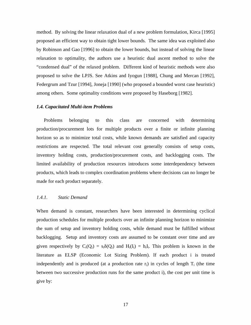
2

)Trd

(1dh

Ts

ci

i

iii

i

ii

−+=

ELSP can then be formulated mathematically by the following constrained objective

function:

ELSP: ∑=Γ∈=

−+

n

1i

ii

iii

i

i

n)1,...,i,(T 2

)Trd

(1dh

Ts

mini

A solution (Ti, i = 1,…, n) is feasible only if in the corresponding production schedules no

two items are produced at the same time. Γ is the set of all feasible solutions.

Nevertheless ELSP has been proved to be NP hard (Hsu [1983]). In his review on ELSP,

Elmaghraby [1978] differentiates between two types of solution procedures: (i) analytical

approaches that find an optimal solution to a restricted version of the problem, and (ii)

heuristic procedures that search for acceptable solutions to the original problem.

1.4.1.1 ELSP analytical approaches

Analytical approaches to solve ELSP restrict Γ to a particular set before solving the

problem. The well known analytical approaches are the common cycle approach due to

Hanssmann [1962] which restrict Γ to (Ti, i = 1,…, n)|Ti = T where T is the length of

the common cycle and the basic period approach due to Bomberger [1966] which restrict

Γ to (Ti, i = 1,…, n)|Ti = NiT where Ni is an integer multiplier of the basic period length

T. Once a feasible basic period length T has been determined (by some search method),

the corresponding multipliers Nj can be determined easily by a dynamic programming

algorithm. Extensions and improvements of the basic period approach can be found in

Elmaghraby [1978], Axsäter [1983], Hendriks and Wessels [1978] and Boctor [1985].

19

1.4.1.2. ELSP heuristic approaches

Most proposed heuristics to solve ELSP require that cycle times be integer multiple of a

basic period. This condition was shown to be a necessary feasibility condition by Boctor

[1982]. Salomon [1991] in his description of “basic period” heuristics showed that they

include three (3) main components: (i) a procedure to compute the parameters Ni and T,

and (ii) a procedure to detect whether a given choice of parameters is infeasible, and (iii) a

rule to modify the multipliers in case of unfeasibility. Since (ii) is NP-Hard (see Hsu

[1983]), the procedures that deal with the feasibility problem are frequently of a heuristic

nature. “Basic period” heuristics were proposed by Madigan [1968], Stankard and Gupta

[1969], Doll and Whybark [1973], Goyal [1973], Saipe [1977], Haessler [1979], Park and

Yun [1984] and Boctor [1985, 1987].

Some interesting variants of the ELSP problem were also studied. Fujita [1978] and

Dobson [1987] worked on the non-zero setup times sequence dependent problem.

Carreno [1990] studied the parallel machine ELSP where m identical machines are

available to process the set of products. The family setup costs, and discounts cases were

studied by Silver and Peterson [1985].

1.4.2 Dynamic demand

In the case of dynamic demands the well-known lot-sizing models that deal explicitly with

capacity restrictions are the Capacitated Lot-Sizing Problem (CLSP), the Continuos Setup

Lot-sizing Problem (CSLP) and the Discrete Lot-sizing and Scheduling Problem (DLSP).

In general, these problems ignore setup times. The definition of these problems is given

in section 1.2.2. The complexity and the solution procedures of the multi-item version of

each of the above mentioned problems are discussed in what follows.

1.4.2.1 The Capacitated Lot-Sizing Problem (CLSP)

Since the multi-item CLSP is NP-Hard (see Chen and Thizy [1987]), little work has been

done to solve the problem optimally. Exact solution procedures have been proposed by a

number of authors. When set-up times are considered, Gelders et al. [1986] and Diaby et

20

al. [1992a] propose a Lagrangean relaxation based Branch and Bound procedure. Barany

et al. [1984] and Leung et al. [1989] use cut-generation techniques within a Branch and

Bound procedure to reach an optimal solution. Eppen and Martin [1987] and Pochet and

Wolsey [1991] propose a stronger formulation of the problem (a formulation with tighter

lower bounds from its linear relaxation problem).

On the other hand, heuristic methods for CLSP were proposed by many authors. Maes

and Van Wassenhouve [1988] classifies these methods in two (2) categories: single

resource heuristics and mathematical programming based heuristics.

The single resource heuristics are of greedy type and can also be divided into two subsets

(as suggested by Salomon): the “period by period” heuristics and the “improvement

heuristics”. The production/procurement plan in the “period by period” heuristics are

determined by finding a plan for period 1 and proceeding up to period T while ensuring

feasibility during the whole process. Such heuristics have been suggested by Eisenhut

[1975], Lambrecht and Vanderveken [1979], Dixon and Silver [1981] and Maes and Van

Wassenhove [1986].

The “improvement heuristics” start with a solution for the complete horizon. This solution

may be infeasible. From this starting solution, feasible production schedules are

generated by simple shifting routines. Such heuristics were suggested by Dogramaci et al.

[1981], Karani and Roll [1982] and Van Nunen and Wessels [1978].

Salomon [1991] divides the mathematical programming heuristics into three categories:

relaxation heuristics, linear programming heuristics and column generation heuristics.

Relaxation heuristics are based on relaxing the “difficult” constraints of the problem.

This relaxation leads to an easier problem that can be solved efficiently. A perturbation

method, in combination with a search procedure, is then used to reach a “good” solution.

Lagrangean relaxation heuristics are proposed by Thizy and Van Wassenhove [1985],

Millar and Yang [1993] (relaxation of the capacity constraints), Chen and Thizy [1987]

(relaxation of demand constraints), among others. Column generation heuristics are based

on set-covering or set-partitioning approaches and can be found in Chen and Thizy [1987]

21

and Cattrysse et al. [1990]. The last, but not the least, are the linear programming

heuristics based on alternative formulations of the problem that have tight linear

relaxation solutions or better structures. Those solutions are then perturbed (if they are not

feasible for the original problem) in different ways to find feasible plans. Linear

programming heuristics can be found in Maes et al. [1989] and Gilbert and Madan [1991].

A different approach based on an item-by-item strategy, which cannot be included in any

of the heuristic categories described above, was proposed by Kirca and Kökten [1994].

Every iteration, a set of items is scheduled over the planning horizon and the procedure

terminates when all items are scheduled. The behavior of some heuristics is examined in

Maes [1987]. In general, single resource heuristics are faster in terms of computational

times than mathematical programming procedures and they are more transparent (easier to

understand). Mathematical programming procedures, on the other hand, tend to yield

solutions of better quality and to be more general.

When setup times are considered, the problem of finding a feasible solution has been

proved to be NP-Hard (Maes et al. [1993]). To deal with this additional complexity,

heuristics that consider setup times allow over-time work options at some costs. Most of

the heuristics available are of the relaxation type and can be found in Billington et al.

[1986], Lozano [1989], Trigeiro et al. [1989], Diaby et al. [1992b], Kirka [1990] (ignores

setup costs) and Mercan and Ereguc [1993] (ignore setup costs and consider a family set-

up time). Backlogging possibilities are allowed by Pochet and Wolsey [1989] and by

Millar and Yang [1993, 1994]. Dixon and Poh [1990] consider a related problem where

capacity constraints are not on production but on storage. Inventories may be constrained

due to limited space or financial resources. Dixon and Poh [1990] proposed a relaxation

heuristic to solve this problem.

1.4.2.2 The Continuous Setup Lot-Sizing Problem (CSLP)

The multi-item CSLP has been studied by Karmarkar and Scharge [1985] who presented a

Branch and Bound procedure to solve it. A Lagrangean relaxation of the capacity

constraints lead to easier subproblems that are solved efficiently within a sub-gradient

22

optimization technique to reach tight lower bounds. An extension to the generic CSLP

that considers parallel machines was studied by De Matta and Guignard [1989] who

proposed a heuristic method based upon a Lagrangean relaxation combined with a greedy

algorithm.

1.4.2.3. The Discrete Lot-Sizing and Scheduling Problem (DLSP)

The multi-item DLSP has been treated by Solomon [1991]. Besides studying the

complexity of some extensions of the generic multi-item DLSP, Solomon [1991]

proposed dynamic programming approaches and heuristics to solve the generic DLSP. He

also proposed two column generation based heuristics for the DLSP with nonzero setup

times. Fleischmann [1990] contributed to solve the problem by a Branch and Bound

algorithm. Lagrangean relaxation and dynamic programming approaches are used to

obtain the lower bounds while the upper bounds are obtained by successive approximation

techniques.

2. Multi-Level Problems

The Multi-Level Lot-sizing Problem (MLLP) considers products that are manufactured or

procured through several levels possibly involving several production/stocking points.

The objective in these problems is to determine a multi-stage production/procurement

schedule which minimizes the total cost while known demand is fulfilled. Relevant costs

consist generally of inventory and production/procurement costs.

There are two types of demand in the MLLP: independent demand and dependent

demand. Independent demand is triggered from outside the firm. Dependant demand is

triggered by the production/supply required to fulfil the independent demand. Dependant

demands create interdependencies between the different items considered in the system

and hence between their planning decisions which make the MLLP a lot more difficult to

solve than the SLP.

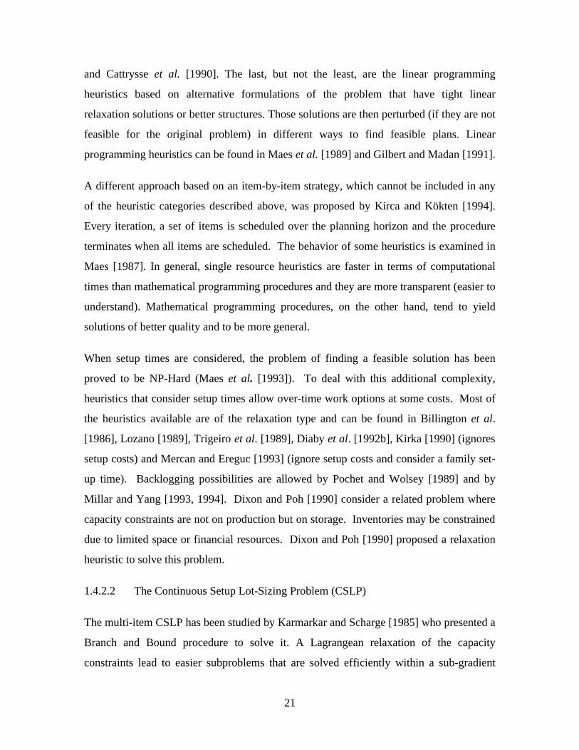
The structure of a multi-level production system can be represented by a directed acyclic

graph, as shown in Figure 4, where nodes represent items and/or stocking points and

23

where arcs describe the relationship between the different nodes. Although a single graph

can be used to represent production and distribution activities, it should be noted that the

nodes-arc structure does not have the same interpretation in both cases. In a production

context, nodes typically represent components which are part of some finished product

(also a node) and the arcs describe the bill of materials with the associated positive

gozinto factors aik (the amount of item i required to produce one unit of item k) and lead-

times iτ . In a distribution structure, the nodes correspond to the stocking points where the

finished products are held and the arcs represent the possible flows between these

locations with their associated lead-times. In a distribution context, all gozinto factors are

equal to one. In what follows, the set of all the nodes in the network is denoted by N,

while the set of immediate successors of an item/stocking point i is represented by Fi, the

number of constrained resources considered in the systems by J and the set of items that

use resource j by Mj.

53

21

4

76

Figure 4: General product structure

Four types of system structures are studied in the literature:

• The serial system structure: each item has at most one successor and one predecessor

(only one end-item can be considered).

24

2

1

3

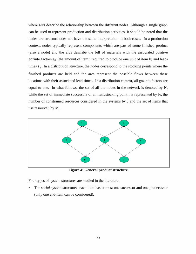
• The assembly product structure: each item has at most one successor (only one end-

item can be considered).

2

1

4 5

3

• The arborescent system structure: each item/location has at most one predecessor

21

4

3

• The general assembly structure: the number of successors and predecessors are not

restricted (Figure 4).

Adapting the notation introduced in Figure 3 to this multi-level context, the MLLP can be

formulated mathematically as a mixed integer program:

25

Min ∑ ∑∑∈ =

τ

=

+

Ni

T

1titit

-T

1titit )(IH)(QC

i

(MLLP)

subject to:

itFk

ktikit1)i(t)-i(t dQaIIQi

i=−−+ ∑

∈−τ T1,..., tN;i +=∈ iτ (MLLP1)

itFk

ktikit1)i(t dQaIIi

=−− ∑∈

− iτ1,..., tN;i =∈ (MLLP2)

u)(QR jtMi

itijj

≤∑∈

T1,..., tJ; ..., 1,j == (MLLP3)

0Q it ≥ T1,..., tN;i =∈ (MLLP4)

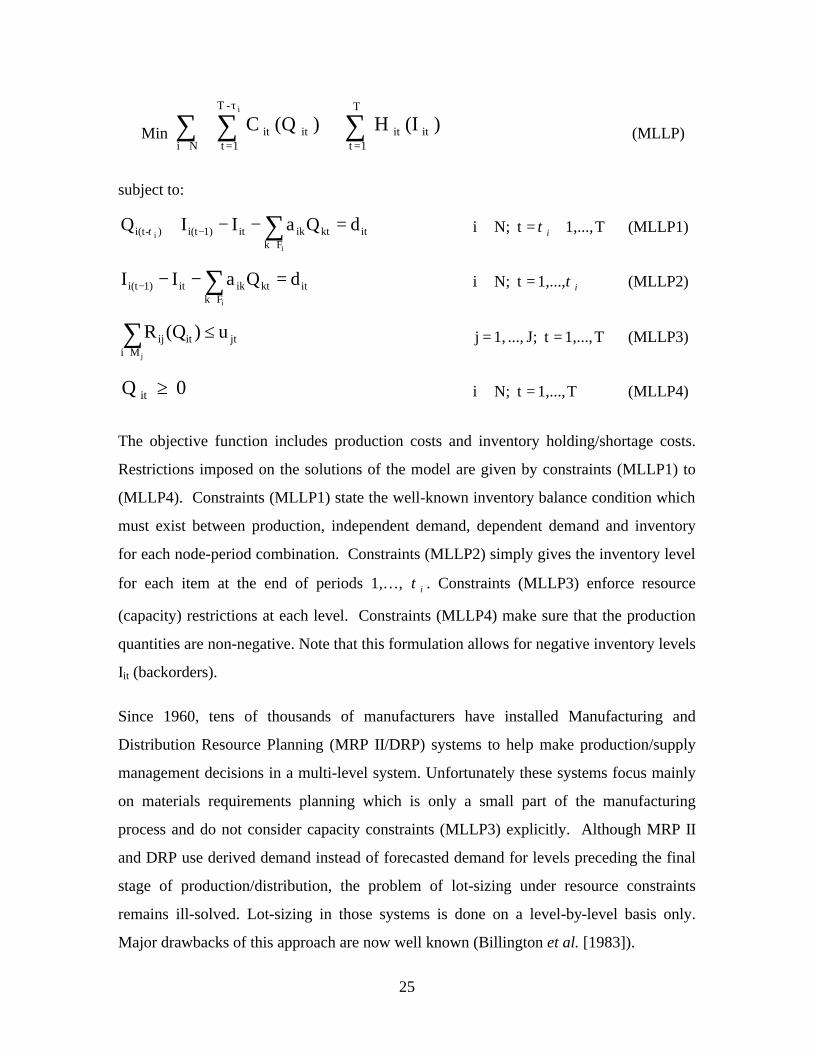
The objective function includes production costs and inventory holding/shortage costs.

Restrictions imposed on the solutions of the model are given by constraints (MLLP1) to

(MLLP4). Constraints (MLLP1) state the well-known inventory balance condition which

must exist between production, independent demand, dependent demand and inventory

for each node-period combination. Constraints (MLLP2) simply gives the inventory level

for each item at the end of periods 1,…, iτ . Constraints (MLLP3) enforce resource

(capacity) restrictions at each level. Constraints (MLLP4) make sure that the production

quantities are non-negative. Note that this formulation allows for negative inventory levels

Iit (backorders).

Since 1960, tens of thousands of manufacturers have installed Manufacturing and

Distribution Resource Planning (MRP II/DRP) systems to help make production/supply

management decisions in a multi-level system. Unfortunately these systems focus mainly

on materials requirements planning which is only a small part of the manufacturing

process and do not consider capacity constraints (MLLP3) explicitly. Although MRP II

and DRP use derived demand instead of forecasted demand for levels preceding the final

stage of production/distribution, the problem of lot-sizing under resource constraints

remains ill-solved. Lot-sizing in those systems is done on a level-by-level basis only.

Major drawbacks of this approach are now well known (Billington et al. [1983]).

26

A review of some of the most important papers published on the different special cases of

the MLLP, depending on demand characteristic (static or dynamic), on capacity

constraints (capacitated or uncapacitated) and on the number of end-items considered

(single or multiple) is presented in what follows.

2.1. Uncapacitated single item problems

In this section we consider MLLP when capacity restriction on resources are not present

and when only one final product is considered. It is usually unrealistic to assume that

resources are unrestricted and available in abundance. However, many approaches to

capacitated multi-level lot sizing and scheduling problems begin by finding lot sizes

without considering capacity constraints. The solution is then modified to eliminate

unfeasibilities. A review of both the static demand and the dynamic demand versions of

the uncapacitated MLLP is provided in the following.

2.1.1. Static demand

Power-of-two policies were proposed to solve single end-item uncapacitated MLLP when

demand is static and an infinite planning horizon is considered. Under a power-of-two

policy, all items are replenished at constant intervals and only when their inventory drops

to zero; moreover the replenishment intervals are all power-of-two multiples of a common

base planning period (lot sizes are allowed to vary from one level to another). With

power-of-two policies it is possible to derive solutions that are very close to optimum

(Roundy [1986]). Such methods can be found in Maxwell and Muckstadt [1985] for

general product structures, in Atkins and Sun [1995] for serial systems (backlogging is

allowed at the final level) and in Sun and Atkins [1997] (backlogging is allowed at the

final level) for assembly systems.

2.1.2. Dynamic demand

The dynamic version of the uncapacitated MLLP is shown to be NP-hard for general

product structures (Arkin et al. [1989]). The production/procurement and inventory

holding costs in the basic version of the problem are time independent and are given

respectively by Ci(Qit) = siδ(Qit) and Hi(Iit) = hiIit. Backlogging is not allowed and

27

independent demands occur for the final product only. The problem is also difficult to

handle from a computational point of view in the sense that straight forward relaxation of

the integrality constraints on setup variables lead to poor quality of lower bounds

(Salomon [1991]). Research on this problem was initiated by Zangwill [1966], Veinott

[1969] and Love [1972]. Most of the work published deals with serial and assembly

systems because of their interesting structure (notice that only one final product can be

considered in the serial and the assembly systems). Those contributions are based on the

“nested” property discovered by Veinott [1969]: if independent demands occur for end

items only, and if production/procurement costs are constant over time, then there exist an

optimal solution to the uncapcitated MLLP for which δ(Qit) = 0 whenever ∑ ∈δ

iFj jt )(Q = 0

(production/procurement cannot occur at one operation unless it also occurs at all of its

immediate successor operations).

When there is no independent demand for components, the serial system is known to be

polynomially solvable by an O(NT4) dynamic programming algorithm (Love [1972]). In

practice the algorithm is of little use, because it requires a large amount of memory and

because the running time grows rapidly with the problem size. The complexity of the

assembly system is still open (Chopra et al. [1997]). Under some assumptions the

assembly system problem is polynomially solvable (see Arkin et al. [1989]).

Exact procedures to solve dynamic uncapacitated MLLP when only one final product is

considered use either dynamic programming, relaxation or reformulation approaches. The

computational effort of the dynamic programming methods increases exponentially with

the problem size, therefore these methods are inefficient for large problems. Dynamic

programming algorithms can be found in Crowston and Wagner [1973] and Zangwill

[1966] for assembly systems. On the other hand, relaxation based procedures generally

use the Lagrangian relaxation technique to obtain an easier problem that can be solved

efficiently. Generally the coupling constraints (MLLP1) are relaxed which leads to easily

solvable shortest path problems. The solution of the relaxed problem is used as a lower

bound in a specialized B&B procedure. Upper bounds are generally obtained by simple

heuristics. Relaxation procedures can be found in Afentakis et al. [1984] and Rosling

[1985] for assembly systems and in Afentakis and Gavish [1986] for general product

28

structures. Reformulation approaches propose more efficient formulations of the problem,

often by using the echelon stock concept. The resulting models can be solved by

specialized cutting plan algorithms exploiting standard optimization software.

Reformulated models are found in Mcknew et al. [1991] and in Clark and Armentano

[1993] (production costs are time-dependent) for assembly systems (independent demand

for components are allowed). Steinberg and Napier [1980], Pochet and Wolsey [1991]

and Clark and Armentano [1993] proposed reformulations for general systems.

Since the computation time and memory required by exact procedures make them useless

for “real-world” cases, several heuristics have been proposed for the problem with general

and assembly product structures. The heuristics proposed in the literature may be divided

into level-by-level, period-by-period and local search methods. The level-by-level

algorithms are based on a decomposition of the problem into single-level subproblems in

combination with cost adaptation procedures that account for interactions between

adjacent levels. Level-by-level heuristics are found in Blackburn and Millen [1982],

McLaren [1976], Graves [1981] and in Coleman and McKnew, [1991] for assembly

systems. In period-by-period heuristics, the solution of the t-time period problem is used

to find the solution of the (t+1)-time period problem. This is repeated till a solution for

the T-time period problem is obtained. This strategy gives to those algorithms the

advantage of controlling the nervousness of the generated policy (Joneja [1991]). Such

heuristics can be found in Afentakis [1987] for assembly systems. Local search techniques

were proposed in Salomon [1991] who used simulated annealing and tabu search to solve

the problem.

2.2. Capacitated single item problems

When capacity restrictions are taken into consideration, the main concern of the MLLP is

to find a production/procurement schedule that minimizes the total cost when demand are

fulfilled and capacity restrictions are respected. Capacity restrictions are generally

considered at one level of the product structure defined as the “bottleneck”. In what

follows, we discuss the single item capacitated MLLP in both the static demand and the

29

dynamic demand cases. The resource consumption function for item i at resource j is

generally assumed to be linear.

2.2.1. Static demand

Several approaches have been proposed to solve a relaxed version (items reorder intervals

are restricted to be integer multipliers of a basic cycle) of the single product capacitated

MLLP when demand is static over an infinite horizon, and when production/procurement

and inventory holdings costs are constant and given respectively by Ci(Qit) = siδ(Qit) and

Hi(Ii) = hiIit. Those approaches may be divided into two classes. The first class consists of

approaches which allow different lot sizes (reorder intervals) for the different

production/procurement levels (Jensen and Khan [1972], Crowston et al. [1973], Schwarz

and Scharge [1975], Williams [1982], Blackburn and Millen [1984], Moily [1986],

Jackson et al. [1988], Karimi [1989], Atkins et al. [1992]). On the other hand,

Szendrovits [1975, 1976] and Goyal [1976], among others assume the same lot size for all

the stages.

2.2.2. Dynamic demand

When demand is time-dependent, an exact procedure to solve the single end-item MLLP

when capacity constraints are considered, and when production/procurement and

inventory holding costs are given respectively by Cit (Qit) = sitδ(Qit) and Hit (Iit) = hitIit, can

be found in Billington et al. [1986]. The paper proposes a B&B algorithm using

Lagrangean relaxation to generate lower bounds, while upper bounds are obtained using

simple smoothing heuristics. Lozano et al. [1989] proposed a primal-dual solution

procedure (includes set-up times).

Heuristic algorithms have attracted more attention than exact procedures. The heuristics

proposed may be divided into three categories: level-by-level, relaxation and cost

adjustment methods. Level-by-level heuristics can be found in Gabbay [1979] when there

are multiple constrained resources and in Zahorik et al. [1984] when there is a single

capacitated resource for serial systems with linear production/procurement costs.

Relaxation heuristics are based on the LP-relaxation of the so-called “facility location”

30

formulation of the MLLP. Such algorithms are proposed by Maes et al. [1991] (include

set-up times), for serial systems, and by Salomon [1991], for assembly systems, who used

the LP relaxation to generate solutions for the problem. Cost adjustment heuristics aim to

adapt some single level heuristics (like the Dixon-Silver procedure) to handle capacitated

multi-level systems. Cost adjustment heuristics can be found in Billington et al. [1989], in

Maes and Van Wassenhove [1991] and in Harrison and Lewis [1996] (minimize inventory

and backorders costs) for serial production environment systems with multiple

constrained resources.

2.3. Uncapacitated multi-item problems

In this section we discuss the uncapacitated MLLP when multiple end-items are

considered in both the static demand and the dynamic demand cases. This problem occurs

generally when general product structures are considered. The production/procurement

and inventory holding costs in the basic version of the problem are given respectively by

Ci(Qit) = siδ(Qit) and Hi(Iit) = hiIit. A literature review of the problem is presented in what

follows.

2.3.1. Static demand

In the static demand case, approaches for solving the uncapacitated multiple end-items

MLLP may be divided into two classes. Approaches of the first class allow different

reorder intervals (lot sizes) for different levels and are generally based on the power-of-

two policy (reoreder intervals are restricted to be a power-of-two multiplier of a basic

cycle). Such methods can be found in Maxwell and Muckstadt [1985], Roundy [1986]

and in Federguen and Zheng [1995] for general product structures where external

demands may occur at any of the network’s nodes and orders are delivered

instantaneously. Power-of-two methods are showed to be within 2% of a lower bound for

the minimum cost even in the case where external demands are allowed for components

and where joint set-up cost is a general monotone submodular function (Roundy [1986]

and Federguen et al. [1992]). Approaches of the second class assume a common reorder

31

interval (lot-size) for all products (Hsu and El-Najdawi [1990]), El-Najdawi and

Kleindorfer (1993)).

2.3.2 Dynamic demand

In the dynamic demand case, we can classify the literature of the uncapcitated MLLP into

two classes. Approaches that solve a restrictive version of the problem optimally and

approaches that propose heuristics procedures to solve the original problem. Approaches

for restrictive versions of the problem can further be divided into two categories: those

that allow different lot sizes for different levels (Afentakis and Gavish [1986]) and those

that impose the same lot-size for the different levels (Karmarkar et al. [1985]).

Few heuristics have been proposed to solve the multiple end-items case. Local search and

relaxation heuristics can be found respectively in Kuik and Salomon [1990] and in

Salomon [1991] for general product structures (independent demand may occur for all

items).

2.4. Capacitated multi-item problems

The capacitated MLLP occurs when production/procurement schedules have to be

determined for multi-level production-inventory systems in the presence of capacity

constraints on resources. In the basic version of the MLLP production/procurement and

inventory holding costs are given respectively by Ci(Qit)= siδ(Qit) and Hi(Iit)= hiIit, only

one bottleneck exists at a given level in the product structure and backlogging is not

allowed. A review of the literature for the static demand and the dynamic demand

versions of this problem are discussed in the following.

2.4.1. Static demand

Research to solve the MLLP when capacity restrictions and multiple end-products are

considered is not very abundant. One of the few contributions to solve this problem, when

demand is static, is Federgruen and Zheng [1993] who generalized the methods proposed

by Maxwell and Muckstadt [1985] and Roundy [1986] by proposing an optimal power-of-

32

two policy for general systems when there is upper and lower bounds on capacity and

bounds on the frequency with which individual items need to be replenished at each level,

and where external demands may occur for components. Hill et al. [1997] proposed

greedy heuristics and an optimal algorithm to solve the problem in the case of a general

system with non-instantaneous lead times and multiple capacity constraints (a capacity

constraint at each level).

2.4.2. Dynamic demand

The MLLP when capacity restrictions and multiple final products are considered is very

hard to solve optimally. When multiple constrained resources are considered, Maes et al.

[1991] proved that simply finding a feasible solution to the multiple end-items case is NP-

Complete. This explains the absence, to our knowledge, of exact procedures to solve this

problem. Some attempts to find a tighter formulation of the problem were made by

Stadtler [1996] (includes setup and overtime). On the other hand, heuristic approaches

have attracted some attention from researchers. The heuristic approaches available can be

divided into relaxation, cost adjustment and local search procedures. Relaxation

heuristics are based on the Lagrangean relaxation techniques. They are found in Billington

et al. [1983] for the single capacity-constrained resource case and in Tempelmeir and

Derstroff [1996] for general product structures and multiple capacity constraints. Cost

adjustment heuristics aim to adapt a single-level procedure (Dixon-Silver [1981]) to solve

the multi-level problem. Such heuristics are found in Tempelmeir and Helber [1994],

Helber [1995] and Katok et al. [1998] who generalized the Harrison and Lewis [1996]

work (single item) to the multi-item case. Local search methods to solve the problem

have been proposed by Salomon et al. [1993] who used simulated annealing and taboo

search techniques.

III. Multi-facility Problems

Multi-facility systems are complex procurement-production-distribution networks

covering a large part of the supply chain. Each plant in the network represents a

multistage system in which the flow of products may be serial, parallel, assembly or

general (Billington et al. [1983]). Lot sizing problems, in this case, are complicated by

the interdependence of different plants.

To reduce the size of the problem, Billington et al. [1983] suggest that in most production

systems there are only a few ‘constrained facilities’ i.e. bottleneck work-centers where

capacity is likely to be a binding constraint so as to cause scheduling difficulties. Thus,

the authors state that lot-sizing is only critical for the constrained work-centers and other

work-centers can often be scheduled on a lot for lot basis. According to this point of view

Karmarkar et al. [1992] reduce a complex manufacturing system into its most critical

‘constrained facilities’ by representing it by what they call an “approximate composite

model”. This representation must be able to capture the salient features of the original

system. Once this is achieved, the very difficult problem described above can be

formulated as a multi-stage lot-sizing problem where each stage is a site. Such

formulations differ from models for multi-stage lot-sizing in a single site since they must

capture the effect of transportation costs between the different sites. Clearly this is a very

difficult problem to solve optimally. However, good heuristics would help quantify the

benefits of coordination as compared to the current practice of optimizing the material

flows plant by plant, which ignores the supply chain sites interdependencies (Bhatnagar et

al. [1993]).

Since the problem is very difficult to solve optimally, only restricted versions of it were

considered by some researchers that attempted to at least evaluate the benefits of

coordination. The constant demand case attracted the attention of most of those

researchers. In particular, three network structures were considered: (1) one origin with

multiple destinations network, (2) multiple origins with one consolidation point and

multiple destinations network, and (3) multiple origins with multiple consolidation points

and multiple destinations network. Since most of the particular cases considered in the

34

literature are treated from a distribution point of view, production capacity constraints are

usually not considered. In the case of dynamic demand, to our knowledge, no work has

been done to solve the coordination problem except the simulation study of Chandra and

Fisher [1994]. In what follows, we present the different multi-facility lot-sizing

coordination problems that were discussed in the literature.

1. Uncapacitated single item problems

In this section we discuss the lot sizing coordination problem when there is no production

capacity constraint and when only a single product is considered in the system.

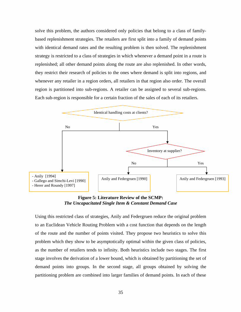
1.1. Static demand

In the case of a single item and static demand, the only structure that was considered is the

one origin and multiple destinations network. Figure 5 summarizes the different

contributions. The one origin multi-destination networks were studied by several authors

who aimed to coordinate production, distribution and transportation decisions. The

products are delivered from the origin by vehicles that combine deliveries to several

retailers into efficient vehicle routes. The objective is to determine replenishment policies

that specify the delivery quantities and the vehicle routes so as to minimize long-run

average production, distribution and transportation costs. Such schedules should specify a

list of routes, the frequency of deliveries on the routes, as well as the lot size for each of

the retailers on the route. Optimal strategies are difficult to find and often very complex

since the problem is related to the classic Vehicles Routing Problem, which is notoriously

NP-Hard (Anily [1986]). Thus, studies on this problem restrict their search to a class of

easily solvable and effective strategies.

Anily and Federgruen [1990] studied the distribution problem of a single product from

one warehouse to geographically dispersed retailers by a fleet of capacitated vehicles. The

warehouse acts as a break-bulk center and does not keep any inventory. Deterministic

constant demand of the products occurs at the retailers. Trucks have a limited capacity,

the holding costs at all the retailers are identical, and the transportation costs consist of a

cost per mile and a fixed cost of hiring a truck. All demands must be met on time. To

35

solve this problem, the authors considered only policies that belong to a class of family-

based replenishment strategies. The retailers are first split into a family of demand points

with identical demand rates and the resulting problem is then solved. The replenishment

strategy is restricted to a class of strategies in which whenever a demand point in a route is

replenished; all other demand points along the route are also replenished. In other words,

they restrict their research of policies to the ones where demand is split into regions, and

whenever any retailer in a region orders, all retailers in that region also order. The overall

region is partitioned into sub-regions. A retailer can be assigned to several sub-regions.

Each sub-region is responsible for a certain fraction of the sales of each of its retailers.

Figure 5: Literature Review of the SCMP:

The Uncapacitated Single Item & Constant Demand Case

Using this restricted class of strategies, Anily and Federgruen reduce the original problem

to an Euclidean Vehicle Routing Problem with a cost function that depends on the length

of the route and the number of points visited. They propose two heuristics to solve this

problem which they show to be asymptotically optimal within the given class of policies,

as the number of retailers tends to infinity. Both heuristics include two stages. The first

stage involves the derivation of a lower bound, which is obtained by partitioning the set of

demand points into groups. In the second stage, all groups obtained by solving the

partitioning problem are combined into larger families of demand points. In each of these

No

No Yes

Yes

Anily and Federgruen [1993]

Identical handling costs at clients?

Inventory at supplier?

Anily and Federgruen [1990] - Anily [1994] - Gallego and Simchi-Levi [1990] - Herer and Roundy [1997]

36

families, efficient vehicle routes are developed using regional partitioning heuristics. The

two heuristics differ in the way the partitioning problem is solved in the first stage. While

the first heuristic uses the average distance from the warehouse to the demand points in a

group as the lower bound for the Traveling Salesman Problem solution for these demand

points, the second heuristic uses twice the maximum distance from the warehouse to a

demand point in the group as the lower bound. For any group of demand points that are

replenished together, an EOQ type formula is derived for the replenishment cost. In their

model, Anily and Federgruen also impose a constraint on the number of demand points

that can be replenished together. They show that both heuristics are asymptotically

convergent. However, asymptotic convergence of the heuristic is guaranteed only when

bounds are imposed on the total demand (number of demand points) that a particular route

can serve.

Anily and Federgruen [1993] extended this work to the case where inventory is kept at the

warehouse as well as at the retailers. Anily [1994] generalized the results to the case

where retailers may have different holding costs and where the warehouse is allowed to

keep inventory. Gallego and Simchi-Levi [1990] treated a similar problem where retailers

are allowed to have different holding costs and a different fixed ordering/transportation

cost. The authors obtain a simple lower bound on the average total cost. Moreover they

show that if the EOQ of each of the retailers is at least 71% of truck’s capacity, then a

simple heuristic using only “direct shipments” (i.e. each route consists of single retailer)

comes within 6% of the lower bound. Herer and Roundy [1997] analyzed the same

problem as Gallego and Levi but with an uncapacitated truck. Herer and Roundy [1997]

used a different approach to solve the problem. The cost function in their model includes

fixed ordering costs and linear inventory costs. The fixed ordering costs are assumed to be

the sum of two cost functions. The first cost function is a given monotone non-negative

submodular function of the set of retailers placing orders at a given point in time. The

second part of the order cost function (i.e. transportation cost) is a per-mile charge times

the length of the traveling salesman tour through the central warehouse and the retailers

that are visited. Inventory costs depend only on the stock at hand, as in the standard EOQ

model. At each point in time when one or more of the retailers place an order, the authors

37

assume that the delivery vehicle follows a traveling salesman tour through the warehouse

and the retailers that are currently placing orders. Under these assumptions, the authors

solve the problem by calculating power-of-two reorder intervals. The main contribution

of Herer and Roundy [1997] is the generalization of Roundy’s [1986] work. They showed

that the cost of the best power-of-two policy is within 2 α percent of the cost of an

optimal policy where the order cost function is α -submodular.

1.2. Dynamic demand

In the case of a single product and a dynamic demand, Diaby and Martel [1993] proposed

a modified Lagrangian relaxation algorithm to solve an arborescent multi-echelon

distribution system. The costs in the multi-echelon system are linear inventory holding

costs and general piece wise linear transportation costs. Using the lagrangian relaxation,

the authors decomposed the problem to two easily solvable sub-problems. The lower

obtained by solving these sub-problems is used in a Branch and Bound algorithm to find

an optimal solution.

Though the paper restricts itself to a specific network structure, and doesn’t consider

production, it is one of the firsts to consider more general network structures with general

piece-wise linear functions.

2. Capacitated single item problems

When the problem is capacitated, the shape of its feasible region is more complex. Thus,

it is more difficult to identify the characteristics of an optimal solution and find a short

cut to reach that ultimate solution as was done by Wagner and Whitin [1958]. When

computer speed and memory was very limited, it was not possible to deal with the

complexity obtained when considering the different facilities interactions at the same

time. Even for the case of a single product and static demand, the capacitated multi-

facility problem remained untackled by the research community. When demand is time

dependent, the problem is more complex. The research community has not yet examined

the flows planning problem in a single item capacitated multi-facility network.

38

3. Uncapacitated multi-item problems

In this section, we present the multi-product version of the lot-sizing coordination

problem for the case where production/distribution capacity is not considered.

3.1. Static demand

For systems where static demand for multiple products is assumed and where resource

capacities in the facilities are not restricted, three categories of supply chain networks

were considered by the research community. The one-origin one-transit one-destination

network, the one-origin multi-destination network and the multi-origin multi-destination

network with one or several transshipment points. A literature review of the flow

coordination problem in these networks when demand is static and multiple products are

considered is presented in what follows.

3.1.1. One-origin One-destination Network

Speranza and Ukovich [1994] dealt with the problem of determining the frequencies at

which several products must be shipped on a common link to minimize the sum of

transportation and inventory costs. Several products must be shipped on the same link

using finite capacity vehicles that may leave only at some given discrete times. The

products are produced with known production rates and are required at a different location

(i.e. warehouse, customer) with a consumption rate equal to their production rate. The

inventory cost is linear and is the same in the plant, in the break-bulk (transshipment

point) and in the warehouse. The transportation cost is proportional to the number of

vehicles used for each shipment (constant per truck per trip). Different types of vehicles

can be considered with different capacities and costs. The problem to solve is when to

ship each product and in what quantities in a way that minimizes the sum of transportation

and inventory costs. In addressing this issue, integer and mixed integer linear

programming formulation models of different particular cases of the problem are

proposed.

39

3.1.2. One-origin Multi-destination Network

For the one-origin multi-destination case, Viswanathan and Mathur [1997] studied a

multi-product generalization of the distribution system considered by Anily and

Federgruen [1990]. The authors developed a heuristic that generates a stationary nested

joint replenishment policy. A policy is defined to be stationary if the replenishment of

each item is made at equally spaced points in time, i.e. with constant replenishment

intervals. A policy is said to be nested if whenever the replenishment interval of a given

item is larger than that of another item, the former is an integer multiple of the second. A

product at a specific retailer is referred to as an item, and the same product at different

retailers is considered as different items. Inventories are kept at the retailers, but not at the

warehouse, which acts as a break-bulk center. The problem is formulated as a joint

replenishment problem (JRP) and a simple heuristic is proposed. Since the vehicles are

capacitated, the heuristic groups items in clusters where power-of-two reorder policies are

followed. However, if all the items in a cluster are replenished at the same frequency,

then the common replenishment interval may be a general integer, rather than a power-of-

two multiple of a basic planning period.

3.1.3. Multi-origin Multi-destination Network

The coordination problem when there are multiple origins, multiple destinations and one

or several consolidation points, is to determine the pattern of direct (i.e. directly from the

origin to the destinations) and indirect (i.e. via a consolidation point) shipments that

minimizes the long run average cost. Figure 6 summarizes the major contributions to this

case. Blumenfeld et al. [1985] aim to determine optimal shipping strategies between

origins and destinations by analyzing the trade-offs that exist between transportation,

inventory and production set-up costs for networks with one consolidation terminal. They

assume that the inventory cost is linear, and that it is the same for the whole system (i.e.in

the origins/destinations and in transit). Transportation cost is a fixed function. Inbound

and outbound shipments at the consolidation terminal are independent and the mix of

parts in each shipment is in proportion to the demands. For an origin-destination, only

two options are considered: shipping all parts directly or shipping all parts via the

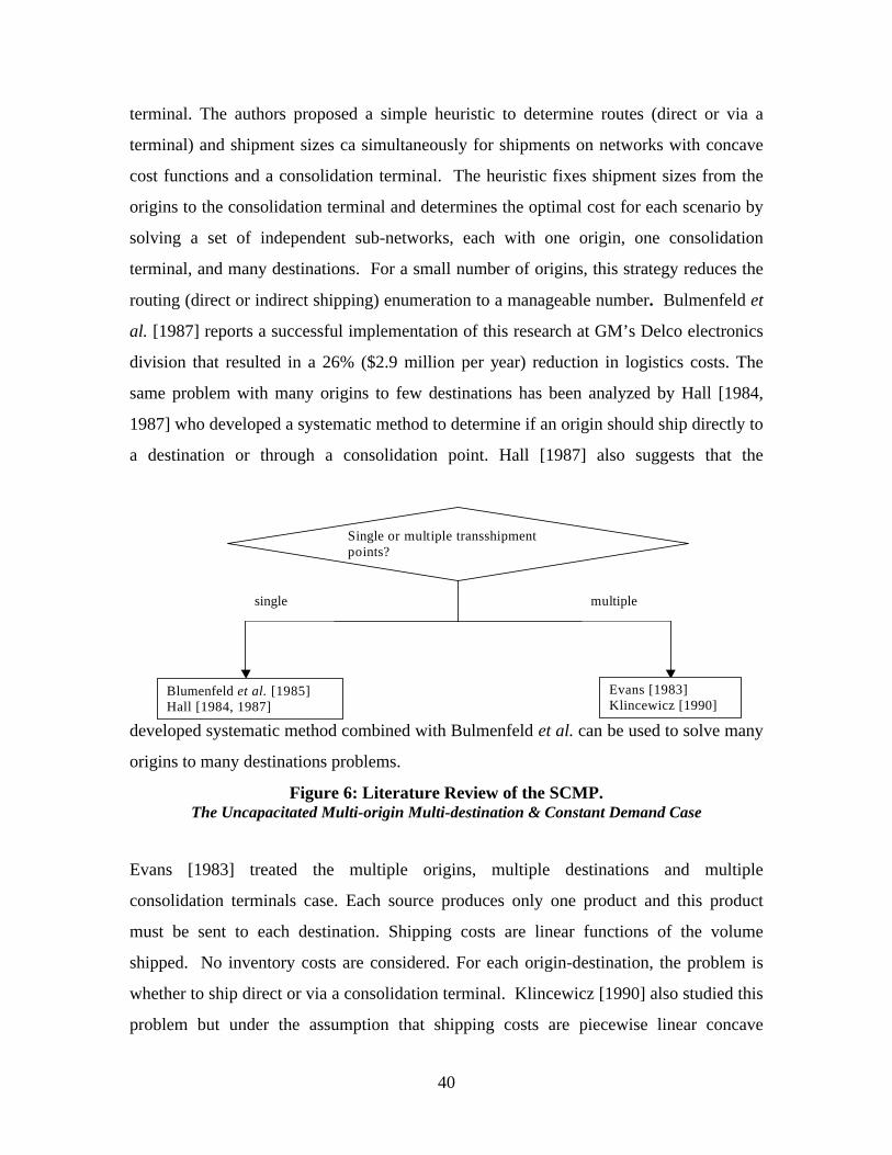
40

terminal. The authors proposed a simple heuristic to determine routes (direct or via a

terminal) and shipment sizes ca simultaneously for shipments on networks with concave

cost functions and a consolidation terminal. The heuristic fixes shipment sizes from the

origins to the consolidation terminal and determines the optimal cost for each scenario by

solving a set of independent sub-networks, each with one origin, one consolidation

terminal, and many destinations. For a small number of origins, this strategy reduces the

routing (direct or indirect shipping) enumeration to a manageable number. Bulmenfeld et

al. [1987] reports a successful implementation of this research at GM’s Delco electronics

division that resulted in a 26% ($2.9 million per year) reduction in logistics costs. The

same problem with many origins to few destinations has been analyzed by Hall [1984,

1987] who developed a systematic method to determine if an origin should ship directly to

a destination or through a consolidation point. Hall [1987] also suggests that the

developed systematic method combined with Bulmenfeld et al. can be used to solve many

origins to many destinations problems.

Figure 6: Literature Review of the SCMP. The Uncapacitated Multi-origin Multi-destination & Constant Demand Case

Evans [1983] treated the multiple origins, multiple destinations and multiple

consolidation terminals case. Each source produces only one product and this product

must be sent to each destination. Shipping costs are linear functions of the volume

shipped. No inventory costs are considered. For each origin-destination, the problem is

whether to ship direct or via a consolidation terminal. Klincewicz [1990] also studied this

problem but under the assumption that shipping costs are piecewise linear concave

Single or multiple transshipment points?

multiple single

Blumenfeld et al. [1985] Hall [1984, 1987]

Evans [1983] Klincewicz [1990]

41

functions of the volume shipped. Klincewicz [1990] solved this problem optimally for

two special cases. In the first case, the sources-to-terminal shipping costs are linear

functions of the volume; in the second case, the terminal-to-destinations shipping costs

are linear functions of the volume. In both cases, the problem may be reduced to a set of

concave cost facility location problems. For more general cases, the author proposed

several heuristics based on solving sequences of the special case with linear costs.

3.2. Dynamic demand

When demand is dynamic and multiple products are considered, the problem gets more

complicated. The lot-sizing process must now take products interaction into account. To

the best of our knowledge, no work has dealt with this problem.

4. Capacitated multi-item problems

The multi-facility problem with capacity constraints, multi-product, and dynamic demand

didn’t attract much interest from the research community. This is mainly due to its

complexity. However, some work has been done to further explain the benefits of

coordinating production, distribution, and routing decisions. Chandra and Fisher [1994]

designed a computational study to investigate the value of coordinating production,

distribution, and routing. Their study involves a plant that produces a number of products

over time and at the same time can hold inventory. The demand for each product at each

retail outlet is known for each period of the planning horizon (dynamic demand) and must

be satisfied without any backlogging. Only one production resource is considered at the

facility and all vehicles have the same capacity; transportation costs is the sum of a fixed

vehicle cost per route in each period t and a cost of direct travel from location to location

(fixed).

The problem is to schedule production and distribution so as to minimize production set-

up, transportation and inventory costs. Production lead times are considered explicitly.

They assume that the operations of the plant can be modeled as a capacitated lot sizing

problem and that the operation of the fleet of vehicles can be modeled as a standard multi-

period local delivery routing problem.

42

The authors’ computational study compares two different ways of managing this system.

The first approach solves production scheduling and vehicle routing problems separately

while the other one coordinates them within a single model. In the decoupled strategy, the

authors first determine a production schedule that minimizes the cost of setups and

inventory subject to meeting total demand per period. This is solved by a cutting plane

algorithm based on Pochet and Wolsey [1991]. They then schedule vehicle deliveries of

products to customers, by the application of some heuristics followed by a local

improvement procedure that attempts to determine whether changing the timing of

customer delivery can reduce costs subject to inventory availability according to the

production schedule. For the coupled production and distribution strategy, a local

improvement heuristic that starts from the decoupled solution and search for cost-reducing

changes is used. The production/distribution schedule with the lowest total cost is taken

to be the new schedule. The process is repeated until no improving changes can be found.

The reduction in total operating costs ranged from 3% to 20%.

The authors indicate that the benefits of coordination increase as the length of the

planning horizon, the number of products and retailers outlet, and vehicle capacity

increases. It is also found beneficial to coordinate these functional activities when

production capacity at the plant (the origin) is less binding, and distribution costs are

higher relatively to the production costs.

Recently, in a Ph.D. thesis at Drexel University, Mallaya [1999] combined supply chain

decisions regarding production plans, delivery quantities and vehicle routing in one

integer-programming model. The objective is to minimize a total cost that includes

production setup costs, linear inventory costs, and linear transportation costs over a finite

planning horizon. Dynamic demand of multiple products needs to be satisfied for each

period of time. In addition, production, inventory and transportation capacities are

considered explicitly in the model. The author proposes a modified Lagrangian approach

to solve the large-size integer-programming problem obtained. Although the author has

spent effort explaining the Lagrangian relaxation approach proposed, no computational

study is included to show the practicability of the approach.

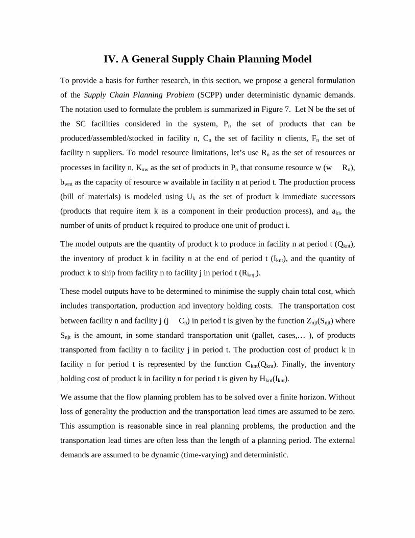
IV. A General Supply Chain Planning Model

To provide a basis for further research, in this section, we propose a general formulation

of the Supply Chain Planning Problem (SCPP) under deterministic dynamic demands.

The notation used to formulate the problem is summarized in Figure 7. Let N be the set of

the SC facilities considered in the system, Pn the set of products that can be

produced/assembled/stocked in facility n, Cn the set of facility n clients, Fn the set of

facility n suppliers. To model resource limitations, let’s use Rn as the set of resources or

processes in facility n, Knw as the set of products in Pn that consume resource w (w ∈ Rn),

bwnt as the capacity of resource w available in facility n at period t. The production process

(bill of materials) is modeled using Uk as the set of product k immediate successors

(products that require item k as a component in their production process), and aki, the

number of units of product k required to produce one unit of product i.

The model outputs are the quantity of product k to produce in facility n at period t (Qknt),

the inventory of product k in facility n at the end of period t (Iknt), and the quantity of

product k to ship from facility n to facility j in period t (Rknjt).

These model outputs have to be determined to minimise the supply chain total cost, which

includes transportation, production and inventory holding costs. The transportation cost

between facility n and facility j (j ∈ Cn) in period t is given by the function Znjt(Snjt) where

Snjt is the amount, in some standard transportation unit (pallet, cases,… ), of products

transported from facility n to facility j in period t. The production cost of product k in

facility n for period t is represented by the function Cknt(Qknt). Finally, the inventory

holding cost of product k in facility n for period t is given by Hknt(Iknt).

We assume that the flow planning problem has to be solved over a finite horizon. Without

loss of generality the production and the transportation lead times are assumed to be zero.

This assumption is reasonable since in real planning problems, the production and the

transportation lead times are often less than the length of a planning period. The external

demands are assumed to be dynamic (time-varying) and deterministic.

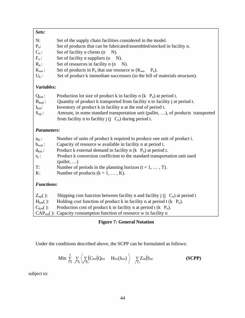
44

Sets:

N: Set of the supply chain facilities considered in the model. Pn: Set of products that can be fabricated/assembled/stocked in facility n. Cn : Set of facility n clients (n ∈ N). Fn : Set of facility n suppliers (n ∈ N). Rn : Set of resources in facility n (n ∈ N). Knw : Set of products in Pn that use resource w (Kwn ⊂ Pn). Uk : Set of product k immediate successors (in the bill of materials structure). Variables:

Qknt : Production lot size of product k in facility n (k∈Pn) at period t. Rknjt : Quantity of product k transported from facility n to facility j at period t. Iknt: Inventory of product k in facility n at the end of period t. Snjt : Amount, in some standard transportation unit (pallet, …), of products transported

from facility n to facility j (j∈Cn) during period t. Parameters:

aki : Number of units of product k required to produce one unit of product i. bwnt : Capacity of resource w available in facility n at period t. dknt : Product k external demand in facility n (k∈Pn) at period t. rk : Product k conversion coefficient to the standard transportation unit used

(pallet, …) T: Number of periods in the planning horizon (t = 1, … , T). K: Number of products (k = 1, … , K). Functions:

Znjt( ): Shipping cost function between facility n and facility j (j∈Cn) at period t Hknt( ): Holding cost function of product k in facility n at period t (k∈Pn). Cknt( ): Production cost of product k in facility n at period t (k∈Pn). CAPwn( ): Capacity consumption function of resource w in facility n

Figure 7: General Notation

Under the conditions described above, the SCPP can be formulated as follows:

Min ( )( ) ( )∑

∑ ∑+∑ +

= ∈ ∈∈

T

1t Nn Cjnjtnjt

Pkkntkntkntknt

nn

SZ)I(HQC (SCPP)

subject to:

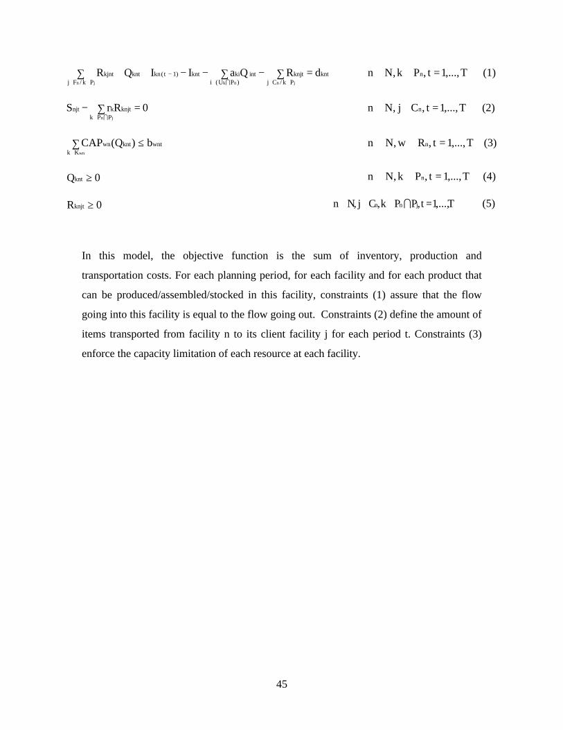
45

kntPk/Cj

knjtPk/Fj )PU(i

intkiknt)1t(knkntkjnt dRQaIIQRjnjn nk

=∑−∑ ∑−−++∈∈∈∈ ∈

−∩

T,...,1t,Pk,Nn n =∈∈∀ (1)

∑ =−∈ jn PPk

knjtknjt 0RrS∩

T,...,1t,Cj,Nn n =∈∈∀ (2)

∑ ≤∈ wnKk

wntkntwn b)Q(CAP T,...,1t,Rw,Nn n =∈∈∀ (3)

0Qknt ≥ T,...,1t,Pk,Nn n =∈∈∀ (4)

0Rknjt ≥ T,...,1t,PPk,Cj,Nn jnn =∈∈∈∀ ∩ (5)

In this model, the objective function is the sum of inventory, production and

transportation costs. For each planning period, for each facility and for each product that

can be produced/assembled/stocked in this facility, constraints (1) assure that the flow

going into this facility is equal to the flow going out. Constraints (2) define the amount of

items transported from facility n to its client facility j for each period t. Constraints (3)

enforce the capacity limitation of each resource at each facility.

46

V. Conclusion

The objective of this paper was to present a unified framework for the research literature

on deterministic flow planning problems. A description and categorization of the most

relevant literature was also presented. Special consideration was given to the multi-facility

flow coordination problem. Important issues for this problem were identified and a novel

formulation for the general problem under dynamic demand was proposed.

It is obvious from the multi-facility section of the paper that several important flow

coordination issues are not studied in the research literature. First, most studies assume

static (deterministic) demand. Little work has been done on the multi-facility problem

when demand is time-dependent, which is the case generally encountered in real life.

Second, the treatment of the production process, if considered, is a gross simplification of

the actual situation. The few models dealing with multi-facility coordination consider,

only single stage manufacturing systems. However, when the product being manufactured

is complex, for example in the case of computers, telecommunication equipment, etc.,

production is often divided between a number of “focused factories”, which cannot be

represented by a single production stage. Third, important savings coming from

economies of scale are not considered in these models. Larger production/purchasing

and/or shipping quantities can lead to major discounts as it has been shown in many

realistic situations. Fourth, only very simple network structures were considered by these

studies, which limit their application.

These shortcomings of the lot-sizing literature are explained mainly by the fact that, in the

past, sales data and information on inventory status at the downstream nodes of the supply

chain were not available for the upstream members, which made it unrealistic for

researchers to include the different actors of the supply chain in their models. Nowadays,

improvements in information and communication technology (e.g. bar coding/scanning,

EDI, Internet) provide many opportunities to increase the efficiency of the total supply

chain. Taking a systems view of the supply chain and integrating its several partners and

actors in the decision making process can lead to a sustainable competitive advantage. In

order to capture the potential of modern information technologies to make better decisions

47

on an enterprise-wide basis and develop win-win strategies, a set of planning and decision

support tools with models that are able to capture the complexity of real production

processes, the saving from economies of scale (specially the ones related to the

transportation costs) and the dynamic nature of demand, is required. Since these models

are NP-hard, the search for tight lower bounds and efficient heuristics is the route to take

from both a practical and a theoretical point view. A generalization of the methods

available to solve single facility lot-sizing problems to procedures capable of tackling

multi-facility problems may yield high payoffs.

48

REFERENCES

1) AGGARWAL, A. and J.K. PARK, “Improved Algorithms for Economic Lot Size

Probelms”, O.R., 41 (1993), 549-571.

2) AFENTAKIS P, B. GAVISH and U. KARMARKAR, “Computationally Efficient Optimal

Solutions to the Lotsizing Problem in Multistage Assembly Systems”, Management

Science, 30 (1984), 222-239.

3) AFENTAKIS, P. and B. GAVISH, “Optimal Lot-Sizing Algorithms for Complex Product

Structures”, O.R., 34 (1986), 237-249.

4) AFENTAKIS, P., “A Parallel Heuristic Algorithm for Lot-Sizing in Muli-Stage

Production Systems. IIE Transactions, (1987), 34-42.

5) ANILY, S., “Integrating Inventory Control and Transportation Planning”, Ph.D

dissertation, Columbia University, New York, (1986).

6) ANILY, S. and A. FEDERGRUEN, “One Warehouse Multiple Retailers Systems with

Vehicle Routing Costs”, Management Science, 36 (1990), 92-114.

7) ANILY, S. and A. FEDERGRUEN, “Two-Echelon Distribution Systems with Vehicle

Routing Costs and Central Inventories”, Operations Research, 41 (1993), 37-47.

8) ANILY, S., “The General Multi-retailer EOQ Problem with Vehicle Routing Costs”,

E.J.O.R., 79 (1994), 451-473.

9) ARKIN, E., D. JONEJA and R. ROUNDY, “Computational Complexity of Uncapacitated

Multi-echelon Production Planning Problems”, Operations Research Letters, 8 (1989),

61-66.

10) ATKINS, D.R. and P.O. IYOGUN, “A Heuristic with Lower Bound Performance

Guarantee for the Multi-Product Dynamic Lot-Sizing Problem”, IIE Transactions,

December (1988), 369-373.

11) ATKINS, D., M. QUEYRANNE and D. SUN, “Lot Sizing Policies for Finite Production

Rate Assembly Systems”, Operations Research, 40 (1992), 126-140.

49

12) ATKINS, D.and D. SUN, “98%-Effective Lot Sizing for Series Inventory Systems with

Backlogging”, Operations Research, 43 (1995), 335-345.

13) AXSÄTER, A., “An Extension of The Extended Basic Period Approach for Economic

Lot Scheduling Problems”, Technical Report, Department of Production Economics,

Link∅ping Institute of Technology, Sweden, 1983.

14) AXSÄTER, A., “Continuous Review Policies for Multi-Level Inventory Systems with

Stochastic Demand”, in Graves et al. Eds., Handbooks in OR & MS, 4 (1993), 175-

197.

15) BAKER K.R., P. DIXON, M.J. MAGAZINE and E.A. SILVER, “An Algorithm for the

Dynamic Lotsize Problem with Time-varying Production Capacity Constraints”,

Management Science, 24 (1978), 1710-1720.

16) BARANY, I., T.J. VAN ROY, and L.A. WOLSEY, “Strong Formulations for Multi-items

Capacitated Lotsizing”, Management Science, 30 (1984), 1255-1261.

17) BASTIAN, M., “Joint Replenishment in Multi-item inventory Systems”, Journal of the

Operational Research Society, 37 (1986), 1113-1120.

18) BERRY W.L., “Lot sizing Procedures for Requirements Planning Systems: a

Framework for Analysis”, Production and Inventory Management, 13 (1972), 19-34.

19) BHATNAGAR, R., P. CHANDRA and S.K. GOYAL, “Models for Multi-plant

Coordination”, European Journal of Operational Research, 67 (1993), 141-160.

20) BILLINGTON, P.J., J.O. MC CLAIN, and L.J. THOMAS, “Mathematical Programming

approaches to Capacity Constrained MRP Systems: Review, Formulation and Problem

Reduction”, Management Science, 29 (1983), 1126-1141.

21) BILLINGTON, P.J., J.O. MC CLAIN, and L.J. THOMAS, “Heuristics for Multilevel Lot-

sizing with a Bottleneck”, Management Science, 32 (1986), 989-1006.

22) BILLINGTON, P.J., J. BLACKBURN, J. MAES, R. MILLEN and L.N. VAN WASSENHOVE,

“Multi-Product Scheduling in Capacitated Multi-Stage Serial Systems”, Technical

50

Report 8908/A, Econometric Institute, Erasmus Universiteit Rotterdam, The

Netherlands, 1989.

23) BITRAN, G. and H.H. YANASSE, “Computational Complexity of the Capacitated Lot

Size Problem”, Management Science, 28 (1982), 1174-1185.

24) BITRAN G. and H. MATSUO, “Approximation Formulations for the Single-Product

Capacitated Lot Size Problem”, O.R., 34 (1986), 63-74.

25) BLACKBURN J.D. and R.A MILLEN, “Improved Heuristics for Multi-Stage

Requirements Planning Systems”, Management Science, 28 (1982), 44-56.

26) BLACKBURN, J.D. and R.A MILLEN, “Simultaneous Lot-sizing and Capacity Planning

in Multi-stage Assembly Processes”, E.J.O.R., 16 (1984), 84-93.

27) BLUMENFELD, D.E, BURNS, L.D., J.D. DILTZ and C.F. DAGANZO, “Analyzing Tradeoffs

between Transportation, Inventory and Production Costs on Freight Networks,

Transportation Research, 19B (1985), 361-380.

28) BLUMENFELD, D.E, BURNS, L.D., C.F. DAGANZO, M.C. FRICK and R.W. HALL,

“Reducing Logistics Costs at General Motors”, Interfaces, 17 (1987), 26-47.

29) BOCTOR, F.F., “Single Machine Lot Scheduling: A Comparison of Some Solution

Procedures”, R. A. I. R. O., 19 (1985), 389-402.

30) BOCTOR, F.F. (1987), “The G-group Heuristic for Single Machine Lot Scheduling”,

International Journal of Production Research, 25 (1987), 363-379.

31) BOMBERGER, E., “A Dynamic Programming Approach to a Lot Size Scheduling

Problem”, Management science, 12 (1966), 778-784.

32) BROWN, R.J., “Decision Rules for Inventory Management”, Holt, Reinhart and

Winston, New York, (1967), 50-55.

33) CARRENO, J.J., “Economic Lot Scheduling for Multiple Products on Parallel Identical

Processors”, Management science, 36 (1990), 348-358.

51

34) CATTRYSSE, D., M. SALOMON, R. KUIK, and L.N. VAN WASSENHOVE, “A Dual Ascent

and Column Generation Heuristic for the Discrete Lotsizing and Scheduling Problem

with Setup Times”, Management Science, 39 (1993), 477-486.

35) CHANDRA, P. and M.L. FISHER, “Coordination of production and distribution

planning”, Journal of the Operational Research Society, 72 (1994), 503-517.

36) CHAKRAVARTY, A.K., “Multi-item Inventory Aggregation into Groups”, Journal of the

Operational Research Society, 32 (1981), 19-26.

37) CHEN, W.H. and J.M. THIZY, “Analysis of Relaxation for the Multi-item Capacitated

Lotsizing Problem”, Technical Report 86-103, School of Management & Department

of Industrial Engineering, State University at Buffalo, N.Y., (1987).

38) CHEN, H., D.W. HEARN, and C. LEE, “A New Dynamic Programming Algorithm for

the Single Item Capacitated Dynamic Lot Size Model”, Research Report 92-7 (1992.a),

Department of Industrial and Systems Engineering University of Florida.

39) CHEN, H., D.W. HEARN, and C. LEE, “A Dynamic Programming Algorithm for

Dynamic Lot Size Models with Piecewise Linear Costs”, Research Report 92-27

(1992.b), Department of Industrial and Systems Engineering University of Florida.

40) CHEN, H., D.W. HEARN, and C. LEE, “A New Dynamic Programming Algorithm for

the Single Item Capacitated Dynamic Lot Size Model”, J. of Global Optimization, 4

(1994), 285-300.

41) Chopra, S., M.R. Rao an C.Y. Tsai, “Computational Study of the Multiechelon

Production Planning Problem”, Naval Research Logistics, 44 (1997), 1-19.

42) CHUNG, C. and C.M. LIN, “An O(T) Algorithm for the NI/G/NI/ND Capacitated Lot

Size Problem”, Management Science, 21 (1988), 420-426.

43) CHUNG, C. and M.H. MERCAN, “A Heuristic Procedure for a Multi-product Dynamic

Lot-Sizing Problem With Coordinated Replenishments”, Working Paper Series (),

March 4 (1992),

44) CHUNG, C., J. FLYNN and C.M. LIN, “An Effective Algorithm for the Capacitated

Single Item Lot Size Problem”, E.J.O.R,, 75 (1994), 427-440.

52

45) COHEN, M., “Joint Pricing and Ordering Policy for Exponentially Decaying Inventory

with Known Demand”, Naval Research Quarterly, 24 (1977), 257-268.

46) COHEN, M. and H. LEE, “Strategic Analysis of Integrated Production – Distribution

Systems: Models and Methods”, O.R., 36 (1988), 216-228.

47) COLEMAN, B.J. and M.A. MCKNEW, “An Improved Heuristic for Multilevel Lot Sizing

Material Requirements Planning”, Decision Sciences, 22 (1991), 136-156.

48) CROWSTON, W. B., M. WAGNER and J.F WILLIAMS, “Economic Lot Size

Determination in Multi-Stage Assembly Systems”, Management Science, 19 (1973),

517-527.

49) CLARK, A.R. and V.A. ARMENTANO, “Echelon Stock Formulation for Multi-stage Lot-

sizing with Component Lead Times”, Int. J. Systems Sci., 24 (1993), 1759-1775.

50) CROWSTON, W. B., M. WAGNER, “Dynamic Lot Size Models for Muti-stage Assembly

Systems”, Management Science, 20 (1973), 14-21.

51) DE MATTA, R. and M. GUIGNARD, “Production Scheduling with Sequence-Independent

Changeover Cost”, Technical Report, Wharton School, University of Pennsylvania,

(1989).

52) DE MATTEIS J.J. and A.G. MENDOZE, “An economic lot sizing technique”, IBM System

Journal, 7 (1968), 30-46.

53) DIABY, M., H.C. BAHL, M.H. KARWAN, and S. ZIONTS, “Capacitated Lot-sizing and

Scheduling by Lagrangean Relaxation”, E.J.O.R., 59 (1992a), 444-458.

54) DIABY, M., H.C. BAHL, M.H. KARWAN, and S. ZIONTS, “A Lagrangean Relaxation

Approach for Very-Large-Capacitated-Scale Capacitated Lot-Sizing”, Management

Science, 38 (1992b), 1329-1340.

53

55) DIABY, M. and MARTEL, A., “Dynamic Lot Sizing for Multi-Echelon Distribution

Systems with Purchasing and Transportation Price Discounts” Operations Research,

41 (1993), 48-59

56) DIXON, P.S. and E.A. SILVER, “A Heuristic Solution Procedure for the Multi-item,

Single Level, Limited Capacity, Lotsizing Problem”, Journal of Operations

Management, 2 (1981), 23-39.

57) DIXON, P.S. and C.L. POH, “Heuristic Procedures for Multi-item Inventory Planning

with Limited Storage”, IIE Transactions, 22 (1990), 112-123.

58) DOBSON, G., “The Economic Lot-Scheduling Problem: Achieving Feasibility Using

Time-Varying Lot Sizes”, Operations Research, 15 (1987), 764-771.

59) DOLL, C.L. and D.C. WHYBARK, “An iterative Procedure for the Single-Machine

Multi-Product Lot Scheduling Problem”, Management Science, 20 (1973), 50-55.

60) EISENHUT, P.S., “A Dynamic Lotsizing Algorithm with Capacity Constraints”, AIIE

Transactions, 7 (1975), 170-176.

61) ELMAGHRABY, S., “The Economic Lot Scheduling Problem (ELSP): Review and

Extensions”, Management Science, 24 (1978), 587-598.

62) El-NAJDAWI, M.K. and P.R. KLEINDORFER, “Common Cycle Lot-size Scheduling for

Multi-product, Multi-stage Production”, Management Science, 39 (1993), 872-885.

63) EPPEN, G.D. and R.K. MARTIN, “Solving Multi-item Capacitated Lot-sizing Problems

Using Variable Redefinition”, Operations Research, 35 (1987), 268-277.

64) ERENGUC, S.S., “Multiproduct Dynamic Lot-Sizing Model with Coordinated

Replenishments”, Naval Research Logistics, 35 (1988), 1-22.

54

65) EVANS, J.R., “A Network Decomposition Aggregation Procedure for a Class of

Multicommodity Transportation Problems”, Networks, 13 (1983), 197-205.

66) FEDERGRUEN, A., M. QUEYRANNE and Y.S. ZHENG, “Simple Power-Of-Two Policies

are Close to Optimal In a General Class of Production/Distribution Networks with

General Joint Setup Costs”, Mathematics of Operations Research, 17 (1992), 951-963.

67) FEDERGRUEN, A., “Centralized Planning Models for Multi-Echelons Inventory Systems

under Uncertainty”, in Graves et al. Eds., Handbooks in OR & MS, 4 (1993), 133-173.

68) FEDERGRUEN, A. and Y.S. ZHENG “Optimal Power-of-Two Replenishment Strategies

in Capacitated General Production/Distribution Networks”, Management Science, 39

(1993), 710-727.

69) FEDERGRUEN, A. and M. TZUR, “The joint Replenishment Problem with Time-Varying

Costs and Demands: Efficient, Asymptotic and ε-Optimal Solutions”, O.R., November-

December (1994), 1067-1086.

70) FEDERGRUEN, A. and Y.S. ZHENG “Efficient Algorithms for Finding Optimal Power-

of-two Policies for Production/Distribution Systems with General Joint Setup Costs”,

Operations Research, 43 (1995), 458-470.

71) FLEISCHMANN, B., “The Discrete Lot-Sizing and Scheduling Problem”, E.J.O.R., 44

(1990), 337-348.

72) FLORIAN, M. and M. KLEIN, “Deterministic Production Planning with Concave Costs

and Capacity Constraints”, Management science, 18 (1971), 12-20

73) FLORIAN, M., J.K. LENSTRA, and A.H.G. RINNOOY KAN, “Deterministic Production

Planning: Algorithms and Complexity”, Management science, 26 (1980), 12-20.

55

74) FRIEDMAN, Y. and Y. Hoch, “A Dynamical Lot-size Model with Inventory

Deterioration”, INFOR, 16 (1978), 183-188.

75) FUJITA, S., “The Application of Marginal Analysis to the Economic Lot Scheduling

Problem”, AIIE Transactions, 10 (1978), 354-361.

76) GABBAY, H., “Multi-Stage Production Planning”, Management Science, 25 (1979),

1138-1148.

77) GALLEGO, G. and D. SIMCHI-LEVI, “On the Effectiveness of Direct Shipping Strategy

for the one Warehouse Multi-retailer R-systems”, Management Science, 36 (1990),

240-243.

78) GASCON, A., “On the finite horizon EOQ model with cost changes”, Operations

Research., 43 (1995), 716-717.

79) GELDERS, L.F., MAES, J., and VAN WASSENHOVE, L.N., “A Branch and Bound

Algorithm for the Multi-item Single Level Capacitated Dynamic Lotsizing Problem”,

in S. Axsaster et al. (eds.), ¨Multi-stage Production Planning and Inventory Control¨,

Lectures Notes in Economics and Mathematical Systems 266, Springer-Verlag, Berlin,

1986, 92-108.

80) GHARE, P., and G. SCHRADER, “A Model for Exponentially Decaying Inventories”,

Journal of Industrial Engineering, 14 (1963), 238-243.

81) GILBERT, K.C., and M.S. MADAN, “A Heuristic for a Class of Production Planning and

Scheduling Problems”, IIE Transactions, 23 (1991), 282-289.

82) GORHAM T., “Dynamic order quantities”, Production and Inventory Management, 20

(1968), 75-81.

83) GOYAL, S.K., “Scheduling a Multi-product Single-machine System”, Operational

Research Quarterly, 24 (1973 (a)), 261-266.

56

84) GOYAL, S.K., “Determination of Economic Packaging Frequency of Items Jointly

Replenished”, ”, Management Science, 20 (1973 (b)), 232-235.

85) GOYAL, S.K., “Determination of Optimum Packaging Frequency of Jointly

Replenished Items”, Management Science, 21 (1974 (a)), 436-443.

86) GOYAL, S.K., “Optimum Ordering Policy for a Multi-item Single Supplier System”, ”,

Operational Research Quarterly, 25 (1974 (b)), 293-298.

87) GOYAL, S.K., “Note on Manufacturing Cycle Time Determination for A Multi-Stage

Economic Production Quantity Model”, Management Science, 23 (1976), 332-333

88) GOYAL, S.K. and S.G. DESHMUKH, “A Note on the Economic Ordering Quantity of

Jointly Replenished Items”, International Journal of Production Research, 31 (1993),

2959-2962.

89) GRAVES, S.C., “Multi-stage Lot-sizing: An Iterative Procedure”, in L.B. Schwartz

(Ed.), Multi-Level Production/ Inventory Control Systems: Theory and Practice, North

Holland, New York, (1981).

90) GRAVES, S.C., “Safety Stocks in Manufacturing Systems”, Journal of Manufacturing

Operations Management, 1 (1988), 67-101.

91) GROFF, K.G., “A Lot sizing rule for time-phases component demand”, Production and

Inventory Management, 20 (1979), 47-53.

92) GUPTA, S.M. and L. BRENNAN, “Heuristic and Optimal Approaches to Lot-sizing

Incorporating Backorders: An Empirical Evaluation”, INT. J. PROD. RES., 30 (1992),

2813-2824.

93) HALL, R.W., “Principles for Routing Freight Through Transportation Terminals”,

Report GMR-5579, General Motors Research Laboratories, Warren, Mich.

57

94) HALL, R.W., “Direct Versus Terminal Freight Routing on a Network with Concave

Costs”, Transportation Research, B21 (1987), 287-298.

95) HANSMANN, F., “Operation Research in Production and Inventory”, John Wiley &

Sons, New York, (1962).

96) HARIGA, M., “Two New Heuristic Procedures for the Joint Replenishment Problem”,

Journal of Operation Research Society, 45 (1994), 463-471.

97) HARISSON, T.P. and H.S. LEWIS, “Lot Sizing in Serial Assembly Systems with Multiple

Constrained Resources”, Management Science, 42 (1996), 19-36.

98) HASEBORG, F., “On the Optimality of Joint Ordering Policies in a Multi-product

Dynamic Lot Size Model with Individual and Joint Set-up Costs”, E.J.O.R., 9 (1982),

47-55.

99) HAX A. C. and D. CANDEA, “Production and Inventory Management”, Printice-Hall,

Inc, Englewood Cliffs, New Jersey, (1984).

100) HELBER, S., “Lot Sizing in Capacitated Production and Control Systems”, Operations

Research Spektrum, 17 (1995), 5-18.

101) HENDRIKS, T.H.B. and J. WESSELS, “Repetitive Schemes for the Single Machine,

Multiproduct Lot-size Problem”, In Proceedings of Operations Research Verfahren

XXVI (1978), 571-581.

102) HERER, Y. and R. ROUNDY, “Heuristics for a One-Warehouse Multiretailer Distribution

Problem with Performance Bounds”, Operations Research, 45 (1997), 102-115.

103) HILL, R.M., “Note: Dynamic Lot Sizing for a Finite Rate Input Process”, Naval

Research Logistics, 44 (1997), 221-228.

104) HILL, A.V., A.S. RATURI and C.C. SUM, “Capacity-Constrained Reorder Intervals for

Materials Requirement Planning Systems”, IIE Transactions, 29 (1997), 951-963.

105) HSU, W., “On the General Feasibility test of Scheduling Lot Sizes for Several Products

on One Machine”, Management Science, 29 (1983), 93-105.

58

106) HSU, J.I.S. and M. El-NAJDAWI, “Common Cycle Scheduling in a Multistage

Production Process”, Engineering Costs and Production Economics, 20 (1990), 73-80.

107) IYOGUN, P. and D. ATKINS, “A Lower Bound and an Efficient Heuristic for Multistage

Multiproduct Distribution Systems”, Management Science, 39 (1993), 204-217.

108) JACKSON, P.L., W.L. MAXWELL and J.A. MUCKSTADT, “Determining Optimal Reorder

Intervals in Capacitated Production-Distribution Systems”, Management Science, 34

(1988), 938-958.

109) JAGANNATHAN, R. and M.R. RAO, “A Class of Deterministic Planning Problems”,

Management science, 19 (1973), 1295-1300.

110) JAIN, K. and E.A. SILVER, “Lot Sizing for a Product Subject to Obsolescence or

Perishability”, E.J.O.R., 75 (1994), 287-295.

111) JENSEN P. A. and KHAN H. A., “Scheduling in a Multistage Production System with

Set-up and Inventory Costs”, AIIE Transactions, 4 (1972), 126-133.

112) JONEJA, D., “The Joint Replenishment Problem: New Heuristics and Case Performance

Bounds”, O.R., 38 (1990), 711-723.

113) JONEJA, D., “Multi-echelon Assembly Systems with Nonstationary Demands:

Heuristics and Worst Case Performance Bounds”, Operations Research, 39 (1991),

512-517.

114) KAO, E.P.C., “A Multi-product Dynamic Lot-Sizing Model with Individual and Joint

Set-Up Costs”, O.R., 27 (1979), 279-284.

115) KARIMI, I.A. (1989), “Optimal Cycle Times in a Two-Stage Serial System with Set-up

and Inventory Costs”, IIE Transactions, 21 (1989), 324-332.

116) KARMARKAR, U.S. and L. SCHRAGE, “The Deterministic Dynamic Product Cycling

Problem”, Operation Research, 33 (1985), 326-345.

117) KARMARKAR, U.S., S. KEKRE, and S. KEKRE, "Lotsizing in Multi-Item Multi-Machine

Job Shops", IIE Transactions, 17 (1985), 290-298.

59

118) KARMARKAR, U.S., S. KEKRE, and S. KEKRE, “The Deterministic Lot Sizing Problem

with Startup and Reservation Costs”, O.R., 35 (1987), 389-398.

119) KARMARKAR, U.S., S. KEKRE, and S. KEKRE, “Multi-item batching heuristics for

minimization of queuing delays”, European Journal of Operational Research, 58

(1992), 99-111.

120) KARNI, R. and Y. ROLLI, “A Heuristic Algorithm for the Multi-item Lotsizing Problem

with Capacity Constraints”, AIIE Transactions, 14 (1982), 249-256.

121) KASPI, M, and M.J. ROSENBLATT, “An improvement of Silver’s Algorithm for the Joint

Replenishment Problem”, IIE Transactions, 17 (1983), 264-267.

122) KASPI, M, and M.J. ROSENBLATT, “The Effectiveness of Heuristic Algorithms for

Multi-item Inventory Systems with Joint Replenishment Costs”, International Journal

of Production Research, 23 (1985), 109-116.

123) KASPI, M, and M.J. ROSENBLATT, “On the Economic Ordering Quantity for Jointly

Replenished Items”, International Journal of production Research, 29 (1991), 107-

114.

124) KIRCA, Ö., “A Heuristic Procedure for the Dynamic Lot-Size Problem with Set-up

Time”, Technical Report, Middle East Technical University, Ankara, Turkey, (1990).

125) KIRCA, Ö., “An Efficient Algorithm for the Capacitated Single Item Dynamic Lot Size

Problem”, E.J.O.R., 45 (1990), 15-24.

126) KIRCA, Ö. and M. KÖKTEN, “A New Heuristic Approach for the Multi-Item Dynamic

Lot Sizing Problem”, E.J.O.R., 75 (1994), 332-341.

127) KIRCA, Ö., “A Primal-Dual Algorithm for the Dynamic Lotsizing Problem with Joint

Set-Up Costs”, Naval Research Logistics, 42 (1995), 791-806.

128) KLINCEWICZ, J.G, “Solving A Freight Transport Problem Using Facility Location

Techniques”, Operations Research, 38 (1990), 99-109.

129) KUIK R. and M. SALOMON, “Multilevel Lotsizing Problem: Evaluation of a Simulated-

Annealing Heuristic”, European Journal of Operational research, 45 (1990), 25-37.

60

130) LAMBERT, A. and H. LUSS, “Production Planning with Time-Dependent Capacity

Bounds”, E.J.O.R., 9 (1982), 275-280.

131) LAMBRECHT, M. and H. VANDERVEKEN, “Heuristic Procedures for the Single

Operation Multi Item Loading Problem”, AIIE Transactions, 11 (1979), 319-326.

132) LASDON L.S. and R.C. TERJUNG, “An efficient algorithm for multi-item scheduling”,

O.R., 19 (1971), 946-969

133) LEE, H. and C. BILLIGTON, “Material Management in Decentralized Supply Chain”,

O.R., 41 (1993), 837-845.

134) LEE, H., PADMANABAHAN V. and WHANG S., “Information Distortion in a Supply

Chain: The Bullwhip Effect”, Management Science, 43 (1997), 546-558.

135) LEV, B. and H.J. WEISS, “Inventory models with cost changes”, O.R., 38 (1990), 53-63.

136) LEUNG, J.M.Y., T.L. MAGNANTI, and R. VACHANI, “Facets and Algorithms for the

Capacitated Lotsizing”, Mathematical Programming, 45 (1989), 331-359.

137) LOVE, S., “A Facilities in Series Model with Nested Schedules”, Management Science,

18 (1972), 327-338.

138) LOZANO, S., “Multilevel Lot-sizing with a Bottleneck Work Center”, Master’s thesis,

Katholieke Universiteit Leuven, Belguim, (1989).

139) MADIGAN, J.C., “Scheduling a Multi-product Single-machine System for an infinite

Planning Period”, Management Science, 14 (1968), 713-719.

140) MAES, J., and L.N. Van WASSENHOVE, “A simple Heuristic for the Multi-Item Single

Level Capacitated Lot Sizing Problem”, Letters of the Operational Research Society, 4

(1986), 265-274.

141) MAES, J., “Capacitated Lotsizing Techniques in Manufacturing Resource Planning”,

Ph.D. thesis, Katholieke Universiteit Leuven, Belguim, (1987).

142) MAES, J., and L.N. Van WASSENHOVE, “Multi-item Single-level Capacitated Dynamic

Lot-sizing Heuristics: a General Review”, Journal of the Operation Research Society,

39 (1988), 991-1004.

61

143) MAES, J., and L.N. Van WASSENHOVE, “Capacitated Dynamic Lotsizing Heuristic for

Serial Systems”, International Journal of Production Research, 29 (1991), 1235-1249.

144) MAES, J., J.O. McClain and L.N. Van WASSENHOVE, “Multilevel Capacitated Lotsizing

Complexity and LP-Based Heuristics”, E.J.O.R., 53 (1991), 131-148.

145) MAGNANTI, T.L., and R. VACHANI, “A Strong Cutting-Plane Algorithm for Production

Scheduling with Changeover Costs”, O.R., 38 (1990), 456-473.

146) Mallya, S.N., “Demand Driven Production and Distribution: Seamless Integration of

Downstream Supply Chain Decisions Using Electronic Data Interchange”, Ph.D

dissertation, Drexel University, (1999)

147) MARTEL, A., “Planning Policies for Multi-Echelons Supply Systems with Probabilistic

Time-Varying Demands”, Publication de Recherche du GREGOR (Groupe de

Recherche en Gestion des Organisations), Institut d’Administration des Entreprises de

Paris-Université Paris 1- Panthéon-Sorbonee. 1995.08.

148) MARTEL, A., M. DIABY, F. BOCTOR, “Multiple Items Procurement Under Stochastic

Nonstationary Demands”, E.J.O.R., 87 (1995), 74-92.

149) MARTEL, A. and A. GASCON, “Dynamic lot-sizing with price changes and price-

dependent holding costs”, to appear in E.J.O.R. (1998).

150) MAXWELL, W.L. and J.A. MUCKSTADT, “Establishing Consistent and Realistic Reorder

Intervals in Production-Distribution Systems”, Operations Research, 33 (1985), 1316-

1341.

151) McLaren, B.J., “Multi-level Lot Sizing Procedures in a Material Requirements

Planning Environnemnt”, Discussion Paper 64, Division of research/School of

Business, Indiana University, (1976).

152) MCKNEW, M.A., C. SAYDAM and B.J. COLEMAN, “An Efficient Zero-One Formulation

of the Multilevel Lot-Sizing Problem”, Decision Sciences, 22 (1991), 280-294.

153) MERCAN, H.M. and S.S. ERENGUC, “A Mult-family Dynamic Lot Sizing Problem with

Coordinated Replenishments: A Heuristic Procedure”, Int. J. Prod. Res., 31 (1993),

173-189.

62

154) MILLAR, H.H. and M. YANG, “An Application of Lagrangean Decomposition to the

Capacitated Multi-item Lot Sizing Problem”, Computers Ops Res., 20 (1993), 409-420.

155) MILLAR, H.H. and M. YANG, “Lagrangean Heuristics for the Capacitated Multi-item

Lot-Sizing Problem with Backordering”, International Journal of Production

Economics, 34 (1994), 1-15.

156) MOILY, J.P., “Optimal and Heuristic Procedures for Component Lot-Splitting in Multi-

Stage Manufacturing Systems”, Management Science, 32 (1986), 113-125.

157) NAHMIAS, S., and S. WANG, “A Heuristic Lot-size Reorder Point Model For Decaying

Inventories”, Management science, 25 (1979), 90-97.

158) PAGE, E., and R.J. PAUL, “Multi-product Inventory Situations with One Restriction”,

Operational Research Quarterly, 27 (1976), 815-834.

159) PARK, K.S. and D.K. YAN, “A Stepwise Partial Enumeration Algorithm for the

Economic Lot Scheduling Problem”, IIE Transactions, 16 (1984), 363-370.

160) POCHET, Y., “Valid Inequalities and Separation for Capacitated Economic Lot Sizing”,

Operations Research Letters, 7 (1988), 109-116.

161) POCHET, Y. and L.A. WOLSEY, “Solving the Multi-item Lot-sizing Problems Using

Strong Cutting Planes”, Management Science, 37 (1991), 53-67.

162) ROBINSON, E.P. and L. GAO, “A Dual Ascent Procedure for Multiprodut Dynamic

Demand Coordinated Replenishment with Backlogging”, Management science, 42

(1996), 1556-1564.

163) ROSLING, K., “Optimal Lot-Sizing for Dynamic Assembly Systems”, Technical Report

152, Link∅ping Institute of Technology, Sweden, 1985.

164) ROUNDY, R., “A 98%-effective Lot-sizing Rule for a Multi-product, Multi-stage

Production/inventory System”, Mathematics of Operations Research, 11 (1986), 699-

727.

63

165) SALOMON, M. (eds.), “Multi-stage Production Planning and Inventory Control”,

Lectures Notes in Economics and Mathematical Systems 355, Springer-Verlag, Berlin,

1991, 92-108.

166) SCHWARZ, L.B. and L. SCHRAGE, “Optimal and System Myopic Policies for Multi-

Echelon Production/Inventory Assembly Systems”, Management Science, 21 (1975),

1285-1294.

167) SENGUPTA, S. and J. TURNBULL, “Seamless Optimization”, IIE Sol., October (1996),

369-373.

168) SHAH, Y., “An Order Level Lot-size Inventory Model for Deteriorating Items”, AIIE

Transactions., 9 (1977), 190-197.

169) SHU, F., “Economic Ordering Frequency for two items Jointly Replenished”,

Management Science, 17 (1971), 406-410.

170) SILVER E.A. and H.C. MEAL, “A heuristic for selecting lot size quantities for the case

of a deterministic time-varying demand rate and discrete opportunities for

replenishment”, Production and Inventory Management, 14 (1973), 64-74.

171) SILVER E.A., “A Simple Method of determining Order Quantities in Joint

Replenishments Under Deterministic Demand”, Management science, 22 (1976),

1351-1361.

172) SILVER E.A., “Coordinated Replenishment of Items Under Time-Varying Demand: A

Dynamic Programming Formulation”, Naval Research Logistics Quarterly, 26 (1979),

141-151.

173) SILVER E.A. and PETERSON, “Decision sysytems for Inventory Management and

Production Planning”, Jhon Wiley & Sons, New York, (1985).

174) SPERANZA, M.G. and W. UKOVICH, “Minimizing Transportation and Inventory Costs

for Several Products on a Single Link”, Operations Research, 42 (1994), 879-894.

175) SUN, D. and D. ATKINS, “98%-Effective Lot-sizing for Assembly Inventory Systems

with Backlogging”, Operations Research, 45 (1997), 940-951.

64

176) STANGARD, M.F. AND S.K. GUPTA, “A Note on Bomberger’s Approach to Lot Size

Scheduling: Heuristic Proposed”, Management science, 15 (1969), 449-452.

177) STADTLER, H., “Mixed Integer Programming Model Formulations for Dynamic Multi-

item Multi-level Capacitated Lotsizing”, E.J.O.R., 94 (1996), 561-581.

178) STEINBERG, E. and H.A. NAPIER, “Optimal Multi-level Lot Sizing for Requirements

Planning Systems”, Management Science, 26 (1980), 1258-1271.

179) SZENDROVITS, A.Z., “Manufacturing Cycle Time Determination for A Multi-Stage

Economic Production Quantity Model”, Management Science, 22 (1975), 298-307

180) SZENDROVITS, A.Z., “On the Optimality of Sub-Batch Sizes for A Multi-Stage EPQ

Model-A Rejoinder”, Management Science, 23 (1976), 334-338.

181) TADIKAMALLA, P.R., “An EOQ Model for Items with Gamma Distributed

Deterioration”, AIIE Transactions, 10 (1978), 100-103.

182) TEMPELMEIER, H. and S. HELBER, “A Heuristic for Dynamic Multi-item Multi-level

Capacitated Lotsizing for General Product Structures”, E.J.O.R., 75 (1994), 296-311.

183) TEMPELMEIER, H. and M. DERSTROFF, “A Lagrangean-based Heuristic for Dynamic

Multilevel Multiitem Constrained Lotsizing with Setup Times”, Management Science,

42 (1996), 738-758.

184) TERSINE R.J. and R.L. PRICE, “Temporary Price Discounts and EOQ”, Journal of

Purchasing and Materials Management, 2nd Quarter (1981), 23-27.

185) THIZY, J.M. and L.N. VAN WASSENHOVE, “Lagrangean Relaxation for the Multi-Item

Capacitated Lotsizing Problem: a Heuristic Implementation”, IIE Transactions, 17

(1985), 308-313.

186) TRIGEIRO, W.W., L.J. THOMAS, and J.O. Mc Clain, “Capacitated Lot Sizing with Setup

Times”, Management science, 35 (1989), 353-366.

187) VAN EIJS, M.J.G., R.M.J. HEUTS and J.P.C. KLEIJNEN, “Analysis and Comparison of

two Strategies for Multi-item Inventory Systems with Joint Replenishment Costs”,

E.J.O.R., 59 (1992), 405-412.

65

188) VAN EIJS, M.J.G., “A Note on the Joint Replenishment Problem under Constant

Demand”, Journal of the Operational Research Society, 44 (1993), 185-191.

189) VAN HOESEL, C.P.M. and A.P.M. WAGELMANS, “An O(T3) Algorithm for the

Economic Lot-sizing Problem with Constant Capacities”, Management science, 42

(1996), 142-150.

190) VAN NUNEN, J.A.E.E. and J. WESSELS, “Multi Item Lot Size Determination and

Scheduling under Capacity Constraints”, E.J.O.R., 2 (1978), 36-41.

191) VAN ZYL, G.J.J., “Inventory Control for Perishable Commodities”, Unpublished Ph.D.

Dissertation, University of North Carolina.

192) VAN WASSENHOVE, L.N. and P. Vanderhenst, “Planning Production in a Bottleneck

Department”, E.J.O.R., 12 (1983), 127-137.

193) VEINOTT, A. F., “Optimal Ordering, Issuing and Disposal of Inventory with Known

Demand”, Unpublished Ph.D. Dissertation, Columbia University, (1960).

194) VEINOTT, A.F., Uunpublished class notes for the Program in Operations Research at

Stanford University, (1963).

195) VEINOTT, A.F., “Minimum Concave Cost Solution of Leontieff Substitution Models of

Multi-Facility Inventory Systems”, O.R., 17 (1969), 267-291.

196) VISWANATHAN, S. and K. MATHUR, “Integrating Routing and Inventory Decisions in

One-Warehouse Multiretailer Multiproduct Distribution Systems”, Management

Science, 43 (1997), 294-312.

197) WAGELMANS, A.P.M., S.V. HOSSEL AND A. KOLEN, “Economic Lot-sizing: An O(n

logn) Algorithm that Runs in Linear Time in the Wagner-Whitin Case”, O.R., 40

(1992), (145-156).

198) WAGNER, H. AND T.M. WHITIN, “Dynamic Version of the Economic Lot Size Model”,

Man. Sci., 5 (1958), 89-96

199) WILDEMAN, R.E., J.B.G. FRENK, R. DEKKER, “An efficient Optimal Solution Method

for the Joint Replenishment Problem”, E.J.O.R., 99 (1997), 433-444.

66

200) WILLIAMS, J.F., “Heuristic Techniques for Simultaneous Scheduling of Production and

Distribution in Multi-Echelon Structures: Theory and Empirical Comparisons”,

Management Science, 27 (1981), 336-352.

201) WILLIAMS, J.F., “On the Optimality of Integer Lot Size Ratios in Economic Lot Size

Determination in Multi-Stage Assembly Systems”, Management Science, 28 (1982),

1341-1349.

202) ZAHORIK, A., L.J. THOMAS and W.W. TRIGERIO, “Network Programming Models for

Production Scheduling in Multi-Stage, Multi-Item Capacitated Systems”, Management

Science, 30 (1984), 308-325.

203) ZANGWILL, W.I., “A Deterministic Multiproduct, Multifacility Production and

Inventory Model”, Ops. Res., 14 (1966), 486-507.

204) ZANGWILL, W.I., “A Backlogging Model and a Multi-Echelon Model of a Dynamic

Economic Lot Size Production System”, Man. Sci., 15 (1969), 506-527.

205) ZOLLER, K. and A. ROBRADE, “Efficient Heuristics for Dynamic Lot Sizing”, INT. J.

PROD. RES., 26 (1988), 249-265.