Lot Sizing at AkzoNobel Polymer Chemicals

Improving the Quantity and Timing of Production Orders

Public

D.J.F. van den Hoogen, Bsc. Industrial Engineering & Management University of Twente (UT) Enschede, 2010

Lot Sizing at AkzoNobel Polymer Chemicals

Improving the Quantity and Timing of Production Orders

Public

D.J.F. van den Hoogen, Bsc. Industrial Engineering & Management University of Twente (UT) Enschede, 2010 Organization: AkzoNobel Polymer Chemicals Stationsstraat 77 Postbus 247 3800 AE Amersfoort Committee: Ir. L.H.F. Hanssen (AkzoNobel) Dr. Ir. J.M.J. Schutten (UT) Dr. Ir. L.L.M. van der Wegen (UT)

1

Preface During the last year, I executed my Master’s assignment at AkzoNobel Polymer Chemicals (ANPC). This report contains the results I obtained during my research. Still, I excluded the information concerning the organization structure, strategy, and most data, since this information is confidential. My research focuses on improving the lot sizing at ANPC; improving the quantity and timing of production orders. The intention is that the results support ANPC in defining the production planning and reducing the lot sizing costs. In addition, by completing this assignment, I complete the Master’s program in Industrial Engineering and Management at the University of Twente. I experienced graduating as a very instructive period. ANPC gave me the opportunity to study an interesting subject and Laurent Hanssen, my supervisor at ANPC, offered me all the support I needed. In addition, Laurent made it possible for me to visit and study different production sites in the Netherlands as well as abroad. I really appreciate that he gave me these opportunities and was never too busy to support me during my research. Also, several employees at ANPC provided me with knowledge and data concerning the production planning and scheduling, inventory management, and other relevant information. For these reasons, I thank these employees, and especially Laurent Hanssen. Furthermore, I want to thank the other people with which I daily enjoyed lunch or a cup of coffee. Next to ANPC, I thank my advisors of the University of Twente, Marco Schutten and Leo van der Wegen, for their support during the execution of my assignment. I experienced their assistance in writing this report as very valuable. Finally, I want to thank my family and friends for their support and interest in this research and during my complete study.

2

Summary Introduction At AkzoNobel Polymer Chemicals (ANPC), production takes place at several production sites across the world. Each production site contains multiple Production Units (PUs) that are only suitable for producing a fraction of the complete product portfolio of ANPC. The production process implies changeover and inventory costs, which we define as the lot sizing costs. Currently, ANPC has insufficient insight in the relation between the decision for the lot sizes and the resulting costs:

1. There is no unambiguous rule regarding how to determine the changeover costs. 2. The validity of the methods that support ANPC in deciding on the lot sizes is unknown. In

this report we define these methods as the current lot sizing policy. In addition, internal research shows that ANPC scores low on inventory costs with respect to the competition. Moreover, AkzoNobel’s Board of Management announced that ANPC should focus on cost reduction, due to the impact of the credit crunch. For this reason, we study the relation between the decision for the lot sizes and the resulting changeover and inventory costs: We study how we can support ANPC in improving the lot sizes and reducing the lot sizing costs. We reflect this need in the goal of our research: To support AkzoNobel Polymer Chemicals in improving the quantity and timing of production orders, in order to reduce the lot sizing costs. Current situation Every week, the Planning Department (PD) of ANPC determines the Production Plan (PP). This PP indicates the quantity and timing of production runs of product families and is determined based on the current lot sizing policy. ANPC classifies a Stock Keeping Unit (SKU) as one product of the total product portfolio and classifies a product family as multiple SKUs with similar chemical characteristics. When deciding on the PP, the PD tries to ensure that the due dates of customers are respected. At the same time, the sum of the production time and the changeover time is limited by the available production capacity of the PU: A changeover between two product families requires a changeover in the PU. Moreover, the inventory levels cannot exceed the available inventory storage capacity for some SKUs, while it is possible to rent or buy additional storage capacity for other SKUs. Consequently, the problem that ANPC faces when deciding on the lot sizes is defined as the Capacitated Lot Sizing Problem (CLSP) with changeover times. Due to the restrictions and the magnitude of the number of product families that ANPC produces in a PU, developing the PP can be quite a puzzle. The PD uses the PP to develop the Weekly Schedule (WS), on SKU level. Heuristic In order to attain our research goal we develop a heuristic that is based on the Simulated Annealing (SA) algorithm, an iterative improvement algorithm. This heuristic calculates a PP for a PU in which the lot sizing costs are minimized, while the capacity restrictions and due dates are respected. We consider the planning on product family level and assume that all data is time-varying, but known with certainty. In accordance with the requirements from ANPC, our heuristic is easy to understand and execute in practice by employees of ANPC. Results We design six different heuristics that are all based on the SA algorithm and calculate the results for twelve different problem instances. In addition, we design two mathematical models that describe the CLSP with changeover times at ANPC and calculate the PP for every problem instance by using optimization software for solving the mathematical models. Next, we compare this output with the output of the heuristics: We compare the lot sizing costs. Unfortunately, the optimization software does not attain the optimal solution for most problem instances. Yet, for two problem instances, which contain five product families, the optimization software does attain the optimal solution. The heuristics approach the optimal solution to respectively 3% and 6%.

3

One heuristic outperforms the other five heuristics. This heuristic, which we define as KK-NS1, first develops a starting solution based on the algorithm of Silver and Meal (1973) and Kirca and Kökten (1992). Next, the heuristic searches for improvements via the SA algorithm by iteratively rearranging two succeeding runs for a product family. The results show that the performance of the heuristic decreases when the number of product families, which need to be included in the PP, increases. In addition, the performance decreases when the demand level increases. Next to assessing the performance of the heuristic by using the output of the optimization software, we analyze whether the heuristic could be used to improve the lot sizing at ANPC: We use the actual data of four PUs and calculate the PP by using KK-NS1. The heuristic attains a valid PP for two problem instances. Following, we compare the lot sizing costs for these valid PPs with the current lot sizing costs: We conclude that the lot sizing costs in both PUs could be decreased with respectively 45% and 15%. For the other two PUs, the heuristic did not attain a valid planning. Yet, we present several possibilities for realizing a valid planning by adapting the demand data. After adapting the demand data, we indicate that the current policy could be improved by 30% and 45% respectively. Still, in practice, adapting the demand could lead to additional costs: We cannot quantify the improvements for these two PUs. Conclusions The results show that our heuristic could be used in decreasing the total lot sizing costs at ANPC. Since the results show a possible cost reduction for two PUs, we recommend that the heuristic is implemented in other PUs as well. There are 31 other PUs around the globe in which the heuristic can be applied. As such, we anticipate that the contribution that the heuristic can deliver, with respect to decreasing the lot sizing cost, is promising. In order to support the implementation of the heuristic, we develop a manual and provide functional training for the end-users.

4

List of abbreviations ANPC AkzoNobel Polymer Chemicals.

BFS Best Found Solution.

CLSP Capacitated Lot Sizing Problem.

CP Cooling Parameter.

CS Cycle Stock.

EOQ Economic Order Quantity.

FCE ForeCast Error.

GBS Global Business Services.

IPC Inventory Penalty Costs.

LB Lower Bound.

LSC Lost Sizing Calculation.

MILP Mixed Integer Linear Problem.

MPOS Minimum Production Order Size.

MTO Make-To-Order.

MTS Make-To-Stock.

NS Neighbourhood Solution.

OR Operations Research.

OS Optimal Solution.

OWC Operating Working Capital.

PC Personal Computer.

PD Planning department.

PI Performance Indicator.

PLT Planned Lead Time.

PP Production Plan.

PU Production unit.

SA Simulated Annealing.

SBU Strategic Business Unit.

SKU Stock Keeping Unit.

SS Safety Stock.

ST Stock Target.

WS Weekly Schedule.

W-W Wagner-Whitin.

5

Contents Preface.............................................................................................................................................2 Summary..........................................................................................................................................3 List of Abbreviations.........................................................................................................................4 Contents...........................................................................................................................................6 Chapter 1 Introduction ............................................................................................................6

1.1 The production process ..............................................................................................6 1.2 Producing to stock ......................................................................................................7 1.3 Goal & research questions..........................................................................................9

Chapter 2 Current situation ...................................................................................................10 2.1 Production planning and scheduling..........................................................................10 2.2 Inventory management .............................................................................................11

2.2.1 Safety Stock .........................................................................................................11 2.2.2 Stock Target.........................................................................................................12

2.3 Quantifying the lot sizing costs..................................................................................13 2.3.1 Changeover costs ................................................................................................13 2.3.2 Inventory costs .....................................................................................................14

2.4 Current policy and current performance ....................................................................15 2.5 Requirements ...........................................................................................................15

Chapter 3 Literature review...................................................................................................17 3.1 The Economic Order Quantity problem .....................................................................17 3.2 The Wagner-Whitin problem .....................................................................................17 3.3 The Capacitated Lot Sizing Problem .........................................................................18 3.4 Capacitated Lot Sizing with Changeover Times ........................................................20

3.4.1 Complexity of the problem ....................................................................................20 3.4.2 Solution methods..................................................................................................20

3.5 Conclusions literature review ....................................................................................23 Chapter 4 Solution design.....................................................................................................25

4.1 Developing two mathematical lot sizing models.........................................................25 4.1.1 Model 1: Discrete operating production units.........................................................25 4.1.2 Model 2: Continuous operating production units....................................................28 4.1.3 Extensions for both Model 1 and Model 2 .............................................................31

4.2 Developing a lot sizing heuristic ................................................................................34 4.2.1 Period-by-period heuristic .....................................................................................34 4.2.2 Simulated annealing .............................................................................................37

Chapter 5 Results & Implications ..........................................................................................40 5.1 Framework ...............................................................................................................40

5.1.1 Problem instances ................................................................................................40 5.1.2 Optimization software ...........................................................................................40 5.1.3 Heuristics .............................................................................................................41 5.1.4 Assessing the results............................................................................................43

5.2 Solving the MILPs.....................................................................................................43 5.2.1 Ability to attain a feasible solution .........................................................................45 5.2.2 Ability to attain the optimal solution .......................................................................46

5.3 Results of the heuristics............................................................................................47 5.4 Assessing the current situation .................................................................................48 5.5 Implications ..............................................................................................................49

Chapter 6 Conclusions & Recommendations ........................................................................54 6.1 Conclusions..............................................................................................................54 6.2 Recommendations....................................................................................................55 6.3 Future research ........................................................................................................55

References................................................................................................................................57 Appendices ...............................................................................................................................60

6

Chapter 1 Introduction The PD within ANPC is responsible for determining the quantity and timing of production orders, which we define as the lot sizing, or determining the lot sizes. At ANPC, the lot sizing results in changeover costs and inventory costs. Currently, there is insufficient insight in the relation between the lot sizing and the resulting (lot sizing) costs. In this chapter we introduce this problem more extensively. First, we present an outline of the production process in Section 1.1, followed by the necessity of producing to stock in Section 1.2. Based on the issues we reveal in Section 1.1 and Section 1.2, we present the goal of our research, the research questions that we should answer to attain our research goal, and the outline of our thesis in Section 1.3.

1.1 The production process At ANPC, production takes place at several production sites across the world. All production sites adhere to strict safety issues, since products can (spontaneously) flame or explode. Each production site contains multiple Production Units (PUs). For example, Deventer locates a production site that contains nine PUs. Some PUs are similar, but most PUs have a unique configuration. As a result, each PU is only suitable for producing a fraction of the complete product range of ANPC. In the remainder of this report we use the term Stock Keeping Unit (SKU) to define a product. ANPC divides SKUs in product groups, called product families. Product families consist of SKUs having similar (chemical) characteristics. The number of product families that ANP produces in a PU varies between approximately one and twenty. The number of SKUs per product family varies between approximately one and thirty. The differences between SKUs within one product family mainly relate to packaging and diluting conditions. For instance, some customers order peroxide in boxes of 25 kg. diluted for 50%, while other customers require the same peroxide in boxes that contain 5 kg., diluted for 40%. ANPC produces SKUs via a two stage production process:

1. A chemical reaction between raw materials inside a reactor that leads to the formation of an end product (family).

2. Diluting and packing the product family, in order to create distinct SKUs. A lot of combinations of packaging material and dilution types are possible.

Although most PUs have a unique configuration, all PUs produce the SKUs according to the two stage production process. The first stage in the production process is the bottleneck. For this reason, ANPC wants to use the capacity of the reactor as efficiently as possible. As mentioned, the PD is responsible for determining the lot sizes; the PD is responsible for utilizing the reactor. The PD schedules two aspects that require the capacity of a reactor: (1) producing a product family, and (2) performing a changeover in the PU, in order to produce another product family. When scheduling a product family for production, the PD needs to take into account that the production process is a batch process: Following the chemical reaction, the process is restarted by draining the product family from the reactor and starting a new batch by adding the raw materials and starting a new reaction. We consider the batch sizes and batch times to be fixed, since:

1. For the chemical reaction to take place and the process to function as defined, a predetermined amount of product needs to be in place.

2. One batch requires a fixed amount of time in order for the reaction to occur. 3. ANPC needs to recalculate the chemical reaction when we want to change batch sizes.

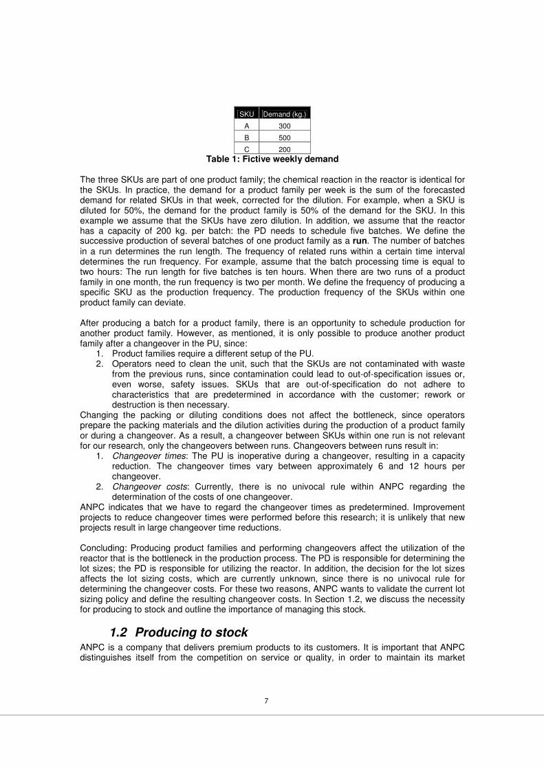
We discuss the necessity for performing a changeover subsequently, but first we present several definitions that ANPC uses via an example: Table 1 presents the fictive weekly demand for three SKUs.

7

SKU Demand (kg.)

A 300

B 500

C 200 Table 1: Fictive weekly demand

The three SKUs are part of one product family; the chemical reaction in the reactor is identical for the SKUs. In practice, the demand for a product family per week is the sum of the forecasted demand for related SKUs in that week, corrected for the dilution. For example, when a SKU is diluted for 50%, the demand for the product family is 50% of the demand for the SKU. In this example we assume that the SKUs have zero dilution. In addition, we assume that the reactor has a capacity of 200 kg. per batch: the PD needs to schedule five batches. We define the successive production of several batches of one product family as a run. The number of batches in a run determines the run length. The frequency of related runs within a certain time interval determines the run frequency. For example, assume that the batch processing time is equal to two hours: The run length for five batches is ten hours. When there are two runs of a product family in one month, the run frequency is two per month. We define the frequency of producing a specific SKU as the production frequency. The production frequency of the SKUs within one product family can deviate. After producing a batch for a product family, there is an opportunity to schedule production for another product family. However, as mentioned, it is only possible to produce another product family after a changeover in the PU, since:

1. Product families require a different setup of the PU. 2. Operators need to clean the unit, such that the SKUs are not contaminated with waste

from the previous runs, since contamination could lead to out-of-specification issues or, even worse, safety issues. SKUs that are out-of-specification do not adhere to characteristics that are predetermined in accordance with the customer; rework or destruction is then necessary.

Changing the packing or diluting conditions does not affect the bottleneck, since operators prepare the packing materials and the dilution activities during the production of a product family or during a changeover. As a result, a changeover between SKUs within one run is not relevant for our research, only the changeovers between runs. Changeovers between runs result in:

1. Changeover times: The PU is inoperative during a changeover, resulting in a capacity reduction. The changeover times vary between approximately 6 and 12 hours per changeover.

2. Changeover costs: Currently, there is no univocal rule within ANPC regarding the determination of the costs of one changeover.

ANPC indicates that we have to regard the changeover times as predetermined. Improvement projects to reduce changeover times were performed before this research; it is unlikely that new projects result in large changeover time reductions. Concluding: Producing product families and performing changeovers affect the utilization of the reactor that is the bottleneck in the production process. The PD is responsible for determining the lot sizes; the PD is responsible for utilizing the reactor. In addition, the decision for the lot sizes affects the lot sizing costs, which are currently unknown, since there is no univocal rule for determining the changeover costs. For these two reasons, ANPC wants to validate the current lot sizing policy and define the resulting changeover costs. In Section 1.2, we discuss the necessity for producing to stock and outline the importance of managing this stock.

1.2 Producing to stock ANPC is a company that delivers premium products to its customers. It is important that ANPC distinguishes itself from the competition on service or quality, in order to maintain its market

8

share. One aspect of delivering premium service to customers is promising a short lead time, and keeping that promise. However, as we explained in the previous section, the production process of ANPC is not flexible, since it is necessary to perform a changeover before producing another product family. As a result, ANPC produces most SKUs to stock, instead of producing SKUs to order, such that ANPC can offer the customers a short lead time, while managing the number of changeovers. MTS implies that capital is caught up in stock, or inventories. This capital cannot be used for other projects, resulting in inventory costs. ANPC uses the term Operating Working Capital (OWC) to define capital that is caught up in short term assets, such as inventories, and values this capital the capital costs. According to Silver et al. (1998), there are six types of inventory:

1. Cycle stock (CS). CS is the result of not matching the quantity and timing of production with the quantity and timing of the demand; producing more than what is actually needed. Since ANPC mainly produces its SKUs to stock, CS is an important part of the total OWC costs: MTS implies higher CS levels in comparison with Make To Order (MTO). Yet, MTS implies a lower number of changeovers. This relation between the number of changeovers and the CS level was first researched by Harris (1913): By decreasing the number of changeovers, the amount of CS increases. Currently, there is insufficient insight in the total changeover and CS holding costs that result from the lot sizing.

2. Anticipatory stock: MTS in order to prepare for seasonal demand. 3. Safety stock (SS). The PD uses forecasts of customer demand to determine the lot sizes.

Still, there is always a deviation between the forecasts and the actual customer orders, defined as the Forecast Error (FCE). SS is an inventory buffer that prevents out-of-stock issues by capturing the FCE. In addition, the SS at ANPC also functions as a buffer for problems in production. Moreover, ANPC uses the SS for strategic reasons for some SKUs. Furthermore, the SS level can be part of a contractual agreement between ANPC and the customers. Finally, for new products or products with irregular demand, there might not be enough data, for example to determine the FCE; in this situation tacit knowledge determines the SS levels to a large extent.

4. Congestion stock. Inventory in the production process, for example when an intermediate product needs to wait for a reactor to become idle.

5. Pipeline stock. Goods in transit. 6. Decoupling stock: When inventory is decentralized (allocated) into different locations,

these locations use this inventory autonomously. This implies that the total inventory throughout the supply chain is higher, because there is less risk pooling1.

There are no prevalent issues regarding seasonal demand, production management, transport management, or allocation management. Yet, we indicated that there is insufficient insight in the total changeover and CS holding costs that result from the lot sizing, while the CS is an important part of the total OWC costs. In the remaining of this report, we refer to CS as the inventory, or the inventory level. We conclude from Section 1.1 and this section that, at ANPC, lot sizing means finding a balance between changeover and inventory costs. However, there is a third cost factor: costs that relate to out-of-stock issues: When ANPC cannot deliver the customers’ order according the due date, customers could cancel the order. It could be possible to change (delay) the order in accordance with the customer, resulting in a backorder, but when customers do not accept backorders, the order becomes a lost sale. Also, backorders have a negative influence on the company image as a trustworthy supplier, while ANPC values this image, as indicated in the beginning of this section. For this reason, we exclude the possibility of out-of-stock issues or backorders from our research; all orders need to be delivered before their due date.

1 Risk pooling: When inventory is stored in a centralized location, the risk of being out-of-stock is lower. This is due to the fact that the deviations between forecasts and actual sales balance on central level: Some customers order more than forecasted, others order less.

9

1.3 Goal & research questions From Sections 1.1 and 1.2, we conclude that ANPC has insufficient insight in the relation between the lot sizing decision and the total changeover and inventory costs. For this reason, ANPC wants to verify whether the lot sizing can be improved. We reflect this need in the goal of our research: To support AkzoNobel Polymer Chemicals in improving the quantity and timing of production orders, in order to reduce the lot sizing costs.

To attain the goal of our research, we need to answer several research questions:

1. What is the current situation regarding the lot sizing? a. How does AkzoNobel Polymer Chemicals determine the lot sizes? b. How can we quantify the changeover and inventory costs? c. What is the current performance regarding the number of changeovers and the

inventory levels? 2. What literature can we use for improving the lot sizing and reducing the total changeover

and inventory costs? 3. How could AkzoNobel Polymer Chemicals improve the lot sizing? 4. What are the implications of applying the improvements in practice?

Before we discuss the outline of this report, we first review the deliverables of our research:

1. Considering the quantity and timing of production runs on product family level; we do not consider the ordering of SKUs within a run. The reason is that the schedule on SKU level does not affect the changeover costs. In addition, the impact on the inventory costs is low, since producing a SKU first, instead of last, in a run only affects the inventory level during the runtime.

2. Improving the quantity and timing of production orders for product families per PU, such that ANPC can use the results for each PU independently.

3. Determining the weekly production plan over a certain time horizon, such that due dates are met, changeover costs and inventory holding costs are minimized, while complying with the maximum production and inventory storage capacity.

In Section 2.5, we discuss how these deliverables result in the requirement for our research: We determine the requirements based on the current situation. We answer the research questions above in the next four chapters of our thesis:

1. Chapter 2: We first describe how ANPC determines the quantity and timing of production orders. Next, we outline the methods that support ANPC in managing the inventories. In addition, we quantify the changeover and inventory costs and present the current performance regarding the number of changeovers and inventory levels. We finalize this chapter by discussing the requirements of our research, and indicating what literature would be relevant to attain those deliverables.

2. Chapter 3: We discuss the literature that is relevant for our research, in accordance with the conclusions from Chapter 2. We conclude Chapter 3 by presenting what literature we could use to support ANPC in determining the lot sizes.

3. Chapter 4: In Chapter 4, we design our solutions in compliance with our conclusions from Chapter 3; we apply the relevant lot sizing literature to the problem that ANPC faces.

4. Chapter 5: Chapter 5 outlines the results of our research. We compare the current performance with the advised situation and analyze the differences: We discuss the implications of applying the improvements in practice.

In Chapter 6 we conclude our research and present whether we attain our research goal and outline our recommendations and possibilities for future research.

10

Chapter 2 Current situation In this chapter, we present the current situation regarding the lot sizing at ANPC. First, we elaborate upon the current methods regarding the lot sizing in Section 2.1 and Section 2.2: In Section 2.1 we discuss into detail how the PD generates a production plan and a production schedule. Next, we describe how ANPC manages their inventories in Section 2.2. Subsequently, in Section 2.3, we discuss the quantification of the changeover and inventory costs. Next, we present the current inventory levels and the number of changeovers in Section 2.4, such that we can compare the current performance with the proposed performance in Chapter 5. In Section 2.5, we conclude Chapter 2 and present the requirements of our research. As such, we point out what literature is relevant for our research.

2.1 Production planning and scheduling The PD uses SAP, an Enterprise Resource Planning system, to support the determination of the production plan and the production schedule. When forecasts indicate that inventory is running out for a SKU, SAP issues one or more production orders for this SKU. These production orders have two main characteristics:

1. Production quantity. All SKUs have a Minimum Production Order Size (MPOS); the production order that SAP generates is at least equal to the MPOS. ANPC installed the MPOSs in order to prevent that SAP generates a lot of small production orders when the inventory is low.

2. Starting date of the production order. SAP subtracts the production time, which depends on the size of the production order, from the moment that the SKU is due for delivery to the customer. For example, when forecasts indicate that the inventory for a SKU runs out on 25-03-2009, and it takes one day to produce this SKU, SAP schedules this SKU for production on 24-03-2009 the latest.

It is the task of the PD to combine the production orders for the SKUs, which SAP generates, in production runs for product families. The PD performs this task by:

1. Defining the PP over a rolling horizon of four to six weeks, on product family level. When determining the PP, the PD makes use of what ANPC defines as the Planned Lead Time (PLT). The PLT represents the time in days between the start of two production runs in which a SKU should be produced. The function of the PLT is to manage the changeover and the inventory costs, which we define as the lot sizing costs in the remainder of this report. As such, the PD tries to determine a planning that respects the due dates and the PLT values for every SKU. Nevertheless, the PP should comply with the available production capacity. In addition, the resulting inventory levels cannot increase above the available inventory storage capacity. As such, determining the planning can be quite a puzzle.

2. When defining the PP, the PD could face several issues, such as delivery issues for raw materials. Consequently, the PD is allowed to deviate from the PLT values to solve possible issues. In addition, capacity issues could be solved in accordance with the Production, Sales, Logistics, or Controlling departments, which we define as the involved departments: Possibilities are to produce certain product families in other PUs, adapt the forecasted demand in accordance with the customers, or buy products from the competition.

3. Defining a Weekly Schedule (WS): Assigning the production orders for the SKUs to the planned production runs; approving the planned orders.

There are several disadvantages of the current method that could negatively affect the lot sizing costs:

1. Currently, ANPC has insufficient insight in the impact of the values for the PLT on the total lot sizing costs. In addition, it is unknown whether the PD can attain a planning that respects the due dates, complies with the available production capacity and the available

11

inventory storage capacity by applying the PLT values. Two years ago, the PLT values were researched, but this research was never finalized.

2. Working with a fixed PLT for all SKUs, while demand is time-varying. To clarify: When the total demand in the PU is low, it could save costs to increase the number of changeovers and produce certain product families more often in shorter runs, since the reactor is idle anyway. On the other hand, when demand is high, it could save costs to decrease the number of changeovers and increase the run length.

Concluding, the PD determines the PP and the WS based on the (fixed) values for the PLTs. The planning and the schedule should comply with the available production capacity and the inventory levels cannot increase above the available inventory storage capacity. In addition, the PD is responsible for the availability of raw materials. However, there is insufficient insight in the impact of (changing) the values for the PLTs on the total lot sizing costs. In addition, it is unknown whether the PD can attain a planning that respects the mentioned constraints, by applying the PLT values. For these reasons, the PD is allowed to deviate from these values. Concluding: ANPC is in need of an analysis of the current PLT values.

2.2 Inventory management We first discuss the SS in Section 2.2.1. Next, we present the use of Stock Targets (STs) for managing the inventory levels and for supporting the determination of the quantity and timing of production orders in Section 2.2.2.

2.2.1 Safety Stock

As indicated in Section 1.2, there is no univocal rule with which the GBS department determines the SS for a SKU. However, the GBS department uses the following formula to calculate a reference value:

With: - MAD: Mean Average Deviation, the average of the absolute difference between the

shipment history and the monthly forecast over a specific time period. The MAD is a measure for the accuracy of the sales forecasts;

- c: A constant functioning as an adjustment of MAD. According to Silver et al. (1998) this constant should equal 1.25 to correctly represent the standard deviation of the ForeCast Error (FCE). This corresponds with the value ANPC applies currently. For more information we refer to Silver et al. (1998);

- k: Safety factor, a measure that represents the chance of delivering a customer from inventory. ANPC applies an identical value for k for every SKU.

We have two remarks concerning how the GBS department uses this formula:

1. We wonder whether applying an identical value for k for all SKUs is correct, since probably some SKUs are more important than other SKUs with respect to, for example, the profit margin or the importance of the customer.

2. As indicated in Section 1.2, ANPC uses the SS for capturing the variation in production, and strategic purposes as well. In addition, there could be a lack of data for calculating the MAD for new SKUs, or SKUs that do not have a regular demand pattern. For these reason, the formula output can be incorrect.

The discrepancy between the output of the formula and reality is reflected in the current way of working: ANPC mainly defines the SSs based on qualitative criteria. For this reason, we do not include the determination of the SS in our research: We focus on the (cycle) inventory costs and the changeover costs. When the results of our research imply that the lot sizing could be improved, ANPC should verify the impact on the changes with respect to the SS.

31***

PLTMADkc

12

Concluding, we assume that all data is time-varying, but known with certainty. In the case of ANPC, uncertainty could arise during production, as well as in the demand pattern. Regarding uncertainty in production, we apply the average availability2 and yield3 data for correcting available production time and batch output, corresponding to the current procedures in the PD. On operational level, there are deviations from these averages, along with the deviations with respect to the forecast accuracy; it is the purpose of the SS to capture these deviations. When necessary, the scheduled production is adapted in order to restore the SS to the intended level. We assume that the SS levels are correct with respect to capturing the deviations and that these deviations cancel out on an aggregate level. As a result, the required production output is identical on an aggregate level, whether or not we take the SS into account in our solution.

2.2.2 Stock Target

Next to the SS, the GBS department determines STs, in order to manage the (cycle) inventory level for every SKU. Every six months, the GBS department calculates the STs based on the results of the last months and the demand forecasts for the coming six months. In comparison to the determination of the SS, there is no univocal rule to determine the STs: Employees from the GBS department determine the new targets based on tacit knowledge. Yet, again, the GBS department uses a reference value: ST = SS + ½ * MPOS. At the end of every month, the GBS department compares the inventory level for every SKU with their ST. When there are large differences, the department analyzes these differences and undertakes action, when necessary. The management of the inventory levels via the use of STs results in some problems:

1. The GBS department evaluates the average inventory levels on a monthly basis, but it is difficult for the PD to plan and schedule production runs such that the inventory levels meet an average target. Due to this reason, the PD does not use the ST when determining the quantity and timing of production orders.

2. There is no insight in the relation between the ST and the total lot sizing costs. As such, the GBS department could decide to decrease the ST, while it would be better to decrease the number of changeovers and increase the ST.

Until now, we only discussed the inventory management for finished goods. The reason is that ANPC experiences no issues regarding the inventory management for the raw materials: It only rarely occurs that the necessary raw materials for producing a planned/scheduled run are lacking. In addition, when the situation occurs in which there are no raw materials, this situation can be solved by issuing rush orders, or modifying the plan/schedule. Also, the SS of finished goods could be used to fulfill the demand. Furthermore, the costs that are involved in ordering and storing the raw materials are lower compared to the changeovers costs and storage costs for the finished goods. Also, the raw materials are mostly stored under ambient conditions in large storage tanks, while the storage of finished goods is more complex, which we indicate in Section 2.3.2. As a result, we assume in our research that the necessary raw materials are available and focus on optimizing the lot sizing costs. On the basis of this research, further research could focus on the possibilities for reducing the costs that occur when managing the inventories of the raw materials. We elaborate on this issue in Section 6.2. In conclusion, the GBS department uses STs to verify the inventory levels. However, the changeover costs are also part of the lot sizing costs; there is no insight in the impact of (changing) the values for the STs on the total lot sizing costs. In addition, the PD does not use the STs when determining the PP and the WS, but uses the PLTs instead, as we showed in Section

2 Availability: A PU faces scheduled (such as maintenance) and unscheduled (among others, breakdowns and operator accidents) downtime. We correct the total number of available hours for the average scheduled and unscheduled downtime. 3 Yield: There always is loss of materials due to cleaning, waste, or other reasons. We correct the theoretical batch output for the average yield.

13

2.1. Since the PLTs and the STs are determined independently and do not reflect the lot sizing costs individually, we expect that the lot sizing at ANPC can be improved. In order to locate these improvement opportunities, we quantify the changeover and inventory costs in Section 2.3.

2.3 Quantifying the lot sizing costs As indicated in Section 1.1, there is no univocal rule for quantifying the changeover costs currently. In addition, we showed in Section 1.2 that ANPC values the inventories against the accompanying capital costs only. However, we question this approach of valuing the inventories, since inventories could also, for example, imply storage or material handling costs. For these reasons, we discussed the quantification of the changeover and inventory costs with employees from the controlling, production, and planning departments: We identified all activities that have an effect on the changeover and inventory costs. Next, we discuss our results.

2.3.1 Changeover costs

Performing a changeover implies: 1. Operator costs: In all production sites under consideration, a flexible number of operators

is available for operating the PUs. Operators perform, among others, changeovers, maintenance, and the monitoring of the different PUs. When there is a changeover in a PU, the production department allocates a number of operators to that PU for cleaning the PU and changing the setup. Since ANPC has a flexible operator workforce, every changeover implies operator costs. We define operator costs as (1) number of operators necessary to perform a changeover * (2) labor costs per operator hour * (3) changeover time.

2. Use of cleaning materials: After a production run of a certain product family, the reactor needs to be cleaned before starting the production of another product family. In addition, for some product families, the operators need to prepare the reactor with certain materials, in order to enable the chemical reaction. We calculate the cleaning costs by multiplying the amount of cleaning materials with the price for the cleaning material.

3. Loss of raw materials: There is always an amount of remaining product in the reactor when operators clean the PU after a production run. For this reason, performing a changeover in order to produce a certain product family implies the loss of raw materials for this product family. This amount depends on the characteristics of the reactor, and is the same for every product family.

When considering a changeover from product family i to product family j, product family j solely determines the cleaning costs: Based on product family j, the reactors require certain preparation for the production process to function properly. In addition, performing a changeover for product family j, implies that there is a loss of raw materials for this product family, when ending the run. In accordance with Trigeiro et al. (1989), we classify the cleaning costs and costs due to the loss of raw materials as sequence independent. The remaining costs aspect, the operator costs, consists of three factors. For the first two factors, (1) number of operators necessary to perform a changeover and (2) labor costs per operator hour, the value is constant per PU; these factors are sequence independent as well. However, when considering the third factor, the changeover time from product family i to product family j, there are exceptions in which the changeover time depends both on product family i as well as product family j, instead of being sequence independent. There are, for example, some product families for which the chemical characteristics or the setup of the PU are quite similar; cleaning or reconfiguring the setup of the PU requires less time, compared to a changeover to another product family. Nevertheless, the PD uses sequence independent changeover times when determining the PP: The PD corrects the available production time for a fixed changeover time per product family. Only when defining the WS, they do take the exceptions regarding the changeover times into account. Before we outline the quantification of the inventory costs, we elaborate upon the implementation of startups and shutdowns in PUs: The product family that is produced first in a week encounters only a startup in that week, and no complete changeover, since a part of the activities already

14

took place during the shutdown in the previous week. Nevertheless, the production department indicates that similar activities need to be performed during a startup and a shutdown, compared to a changeover. As a result, producing a certain product family implies that the total costs increase with the changeover costs; it is not necessary to determine startup or shutdown costs independently.

2.3.2 Inventory costs

The inventory costs are sometimes referred to as opportunity costs, since it is not possible to use the capital that is caught up in inventories in some other financial productive way. Coyle et al. (2003) indicate that the capital costs most often embody the largest component of total inventory costs. However, the costs that relate to administration and handling, storage (buildings and land), obsolescence (shelf-life of SKUs), or insurance for theft and damage also determine the inventory costs. ANPC uses the following reasoning for not taking these additional costs into account:

1. Administration and handling: ANPC divides the administration and handling in three basic steps: (1) administrate production output, (2) transfer output to storage and administrate the storage, and (3) transfer SKUs to transport and administrate the sale. The most important factor that determines administration and handling costs is the sales level. After all, when there are no sales, it is not necessary to produce, administrate, or handle SKUs, while the necessary administration and handling tasks increase when the sales increase. On the other hand, the administration does not increase when the inventory level increases, since there is no additional administration. We could argument that the handling increases, but ANPC indicates that this additional handling is negligible. However, there is no data available that can support this argumentation.

2. Storage: ANPC divides the storage buildings at the production sites in three categories. The first category of buildings stores SKUs between -10 and -20 ºC, the second between -10 and 10 ºC, and the third encompasses ambient storage. Only when an entire storage building can be made redundant for a long time period, ANPC would consider the possibility of renting the free space to third parties. However, the strict safety rules across the sites do not support renting redundant storage space to third parties. For this reason, decreasing the inventory levels does not imply that the inventory costs decrease as well: The storage costs are fixed, independently of the inventory level. Still, when the inventory level increases above the storage capacity limit, ANPC could consider renting additional storage capacity.

3. Obsolescence: In general, SKUs do not expire in less than one year. In addition, ANPC can choose to reprocess slow movers4. This has a small impact on production costs. Only when reprocessing is not possible and slow movers need to be destroyed, ANPC faces obsolescence costs. However, there is no information of these costs at the production sites that we consider in our research, since destroying slow movers rarely occurs. As a result, ANPC does not take the costs for obsolescence into account when determining the inventory costs.

4. Insurance: Insurance costs for theft and damage mainly relate to capital intensive goods, such as buildings or machines.

Another discussion regarding the determination of the inventory costs comprises the question of how to define the inventory value. Coyle et al. (2003) point out that relevant research indicates that the capital costs should only be applied to the out-of-pocket investment in inventory: The direct variable expense of having inventory in storage. In other words, raising or lowering the inventory levels financially affects the variable costs of inventory value; not the fixed costs. ANPC currently values the capital costs against the cost price of a SKU; the fixed and variable costs. This implies that the method of defining the inventory value might overrate the inventory costs. Variable costs comprise the costs of the raw materials. To conclude this section: 4 Slow movers: SKUs that remain in storage for more than half a year.

15

1. By defining the inventory costs with solely the capital costs, ANPC might underrate the inventory costs. However, according to Coyle et al. (2003), the capital costs most often embody the largest component of total inventory costs. This statement applies to ANPC, since the relation between the inventory level and the storage, obsolescence, and insurance costs is low: Only handling costs might have to be allocated (partly) based on the inventory level. As a result, we state that the magnitude of the error is low.

2. By defining the inventory value with the fixed and variable costs, ANPC is overrating the inventory costs.

Summarizing, ANPC overrates the inventory value, but (partly) offsets this by only pricing the inventory value for the capital costs; neglecting administration and handling costs. Consequently, we judge this approach as quite accurate; we will not research the relation between the administration and handling costs and the inventory level into more detail, but determine the inventory costs in accordance with ANPC. Yet, before presenting the current policy and performance in the next section, we mention that when the inventory level increases above the storage capacity limit, ANPC could have the opportunity to rent additional storage capacity: At some sites, ANPC cannot store certain SKUs at third parties, due to safety restrictions. We indicate how we deal with these additional costs in Section 4.1.3.

2.4 Current policy and current performance In our research we consider the lot sizing in four distinct PUs. We refer to these PUs as:

1. PU1. 2. PU2. 3. PU3. 4. PU4.

The PUs differ on, among others, the number of product families that are produced, location, and production capacity. Another difference is that PU1 and PU2 only operate for five days a week; there is a shutdown on Friday and a startup at the beginning of the next week. We define these PUs as discrete units. On the contrary, the remaining two PUs operate seven days a week; there is no necessity for startups or shutdowns in the weekend. We define these PUs as continuous units. We present more information regarding these four PUs in Chapter 5. We do not present the lot sizing data in this report, since this data is confidential. Still, we introduce some definitions:

1. Current performance: The number of changeovers and the average inventory levels per product family during 2008.

2. Current policy: We showed in Section 2.1 that the PD determines the planning and the schedule based on the PLTs. In addition, we showed in Section 2.2 that the GBS department manages the inventories by using the STs. For this reason, the current policy consists of the PLTs and the STs. Regarding the current policy, we use the data applicable to the last 26 weeks of 2009.

2.5 Requirements From Section 2.1 and 2.2, it became apparent that the current lot sizing policy consists of determining the planning by using the PLTs and verifying the inventory costs by using the STs. However, ANPC does not know whether the PLTs reflect the determination of a planning with minimal lot sizing costs. In addition, the verification based on the STs is not complete, since the changeover costs are also part of the lot sizing costs. For these reasons, we will develop a tool that calculates a planning, which we define as the advised planning, that minimizes the total changeover and inventory costs, while meeting the forecasted demand and complying with the maximum production and inventory storage capacity. The PD could use this planning in defining the PP. In addition, the GBS department could use the results in order to validate the current values for the PLTs and the STs, such that they could define valid targets. This tool should comply with the following requirements:

16

1. Being understandable and easy to use for the employees of ANPC. A direct result is that the tool is programmable in Microsoft Excel. The reason is that ANPC has a license to use Microsoft Excel. In addition, the employee who will perform the follow-up on our research has experience with programming in Microsoft Excel.

2. ANPC aims for a tool that presents its output in less than 900 seconds, in order to increase the practicability of the tool.

3. Determining the planning over a time horizon of six months, since this horizon complies with the GBS review period: Every six months, the values for the STs are reviewed by the GBS department. We will verify the results of the tool for a time horizon of six months, and indicate whether the tool gives satisfying results.

4. Dividing the time horizon in weekly buckets, since the PD determines the planning on a week-by-week basis.

In Chapter 3, we consider how we can attain our requirements by discussing the relevant literature.

17

Chapter 3 Literature review In this chapter we present the lot sizing problems and solutions that are defined in the lot sizing literature and that relate to the problem that we face at ANPC. Kuik and Salomon (1994) and Jans and Degraeve (2005) give extensive reviews of a large part of the lot sizing literature; we refer the interested reader to their work.

3.1 The Economic Order Quantity problem One of the first lot sizing problems defined in the lot sizing literature is the Economic Order Quantity (EOQ) problem. The problem consists of finding the order quantity that minimizes the ordering and inventory holding costs under the following assumptions:

1. Single item (SKU or product family) environment; 2. Unlimited capacity, for example unlimited production capacity or inventory storage

capacity; 3. Constant parameters, such as demand, ordering costs, and inventory costs; 4. Zero lead time; 5. No allowance of shortages.

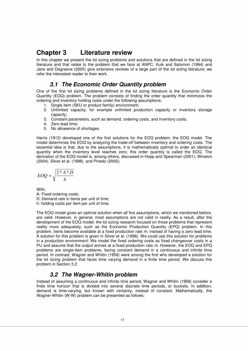
Harris (1913) developed one of the first solutions for the EOQ problem: the EOQ model. The model determines the EOQ by analyzing the trade-off between inventory and ordering costs. The essential idea is that, due to the assumptions, it is mathematically optimal to order an identical quantity when the inventory level reaches zero; this order quantity is called the EOQ. The derivation of the EOQ model is, among others, discussed in Hopp and Spearman (2001), Winston (2004), Silver et al. (1998), and Pinedo (2005):

h

DAEOQ

**2=

With, A: Fixed ordering costs; D: Demand rate in items per unit of time; h: holding costs per item per unit of time. The EOQ model gives an optimal solution when all five assumptions, which we mentioned before, are valid. However, in general, most assumptions are not valid in reality. As a result, after the development of the EOQ model, the lot sizing research focused on those problems that represent reality more adequately, such as the Economic Production Quantity (EPQ) problem. In this problem, items become available at a fixed production rate m, instead of having a zero lead time. A solution for this problem is given in Silver et al. (1998). We could use this solution for problems in a production environment: We model the fixed ordering costs as fixed changeover costs in a PU and assume that the output arrives at a fixed production rate m. However, the EOQ and EPQ problems are single-item problems, facing constant demand in a continuous and infinite time period. In contrast, Wagner and Whitin (1958) were among the first who developed a solution for the lot sizing problem that faces time varying demand in a finite time period. We discuss this problem in Section 3.2.

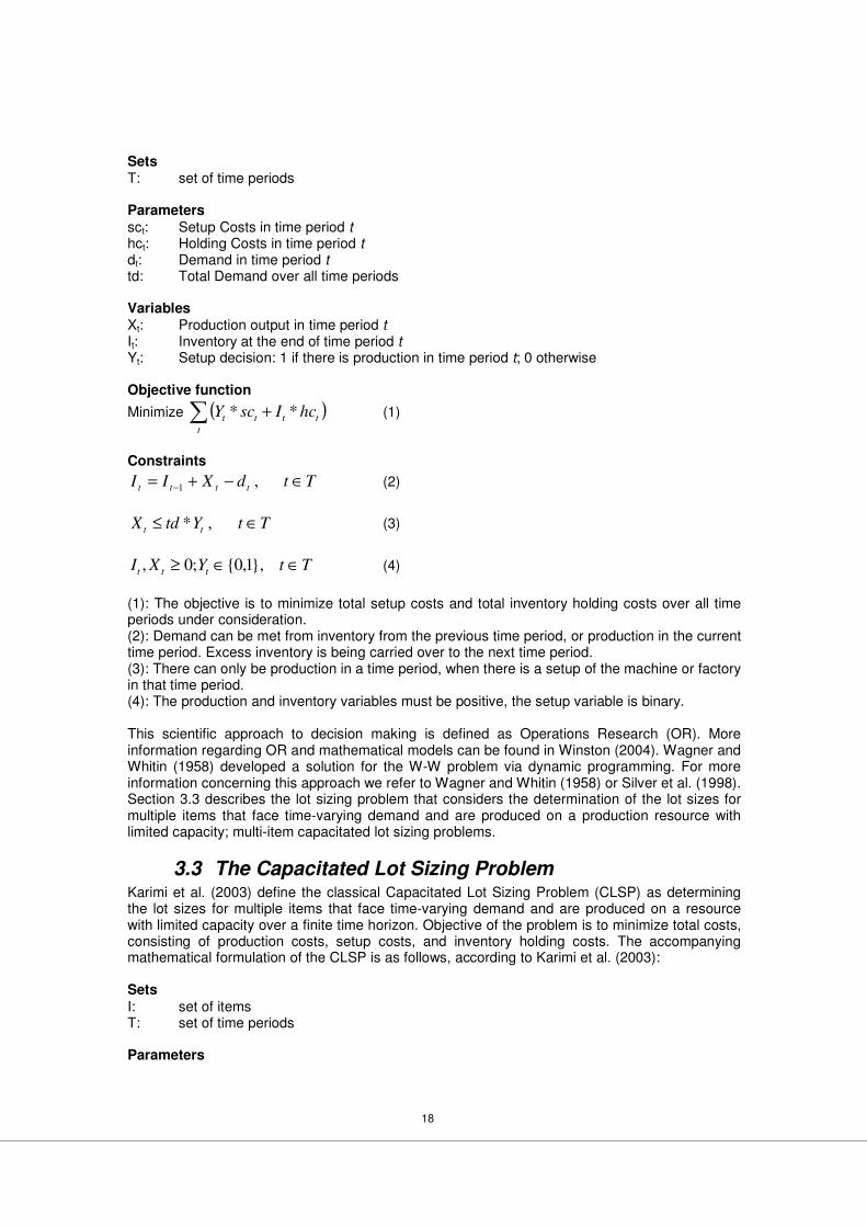
3.2 The Wagner-Whitin problem Instead of assuming a continuous and infinite time period, Wagner and Whitin (1958) consider a finite time horizon that is divided into several discrete time periods, or buckets. In addition, demand is time-varying, but known with certainty, instead of constant. Mathematically, the Wagner-Whitin (W-W) problem can be presented as follows:

18

Sets T: set of time periods Parameters

sct: Setup Costs in time period t hct: Holding Costs in time period t dt: Demand in time period t td: Total Demand over all time periods Variables Xt: Production output in time period t It: Inventory at the end of time period t Yt: Setup decision: 1 if there is production in time period t; 0 otherwise Objective function

Minimize ( )∑ +t

tttt hcIscY ** (1)

Constraints

TtdXII tttt ∈−+=−

,1

(2)

TtYtdX tt ∈≤ ,* (3)

TtYXI ttt ∈∈≥ ,}1,0{;0, (4)

(1): The objective is to minimize total setup costs and total inventory holding costs over all time periods under consideration. (2): Demand can be met from inventory from the previous time period, or production in the current time period. Excess inventory is being carried over to the next time period. (3): There can only be production in a time period, when there is a setup of the machine or factory in that time period. (4): The production and inventory variables must be positive, the setup variable is binary. This scientific approach to decision making is defined as Operations Research (OR). More information regarding OR and mathematical models can be found in Winston (2004). Wagner and Whitin (1958) developed a solution for the W-W problem via dynamic programming. For more information concerning this approach we refer to Wagner and Whitin (1958) or Silver et al. (1998). Section 3.3 describes the lot sizing problem that considers the determination of the lot sizes for multiple items that face time-varying demand and are produced on a production resource with limited capacity; multi-item capacitated lot sizing problems.

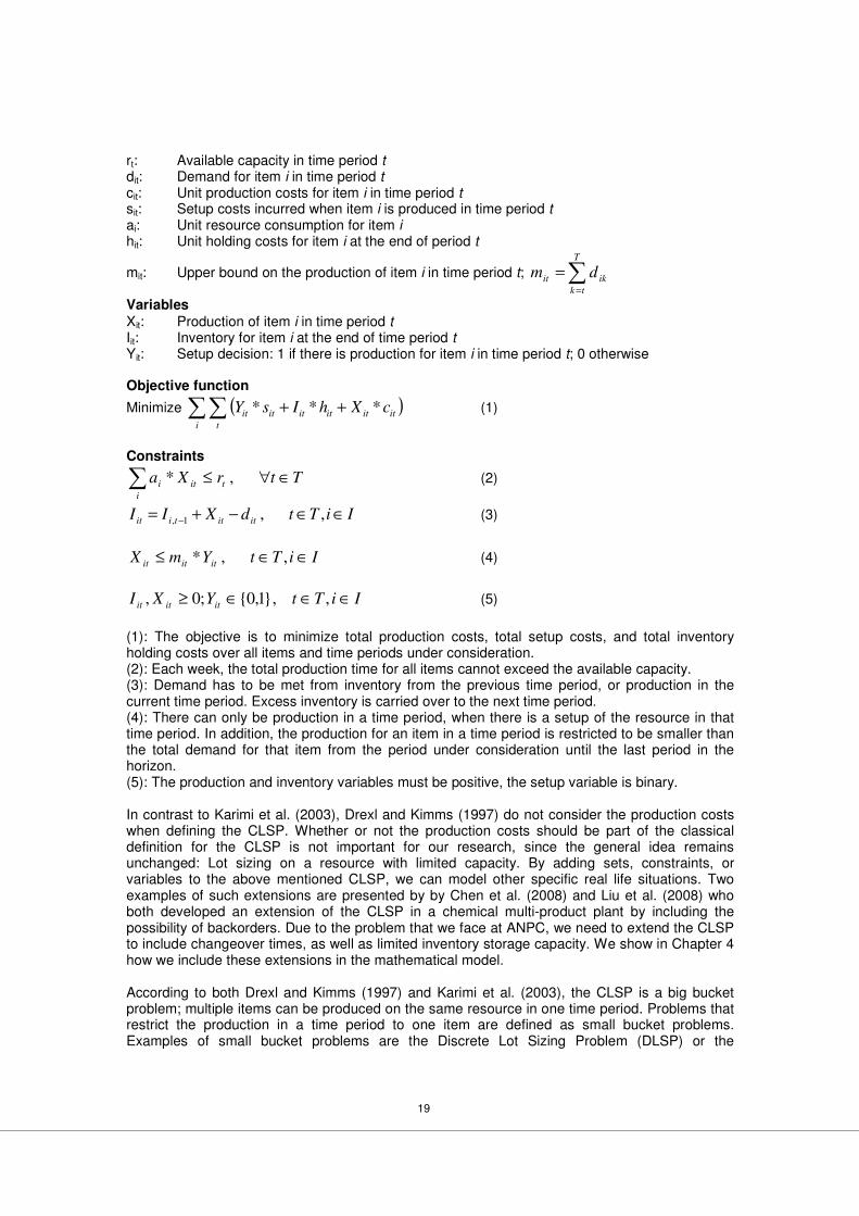
3.3 The Capacitated Lot Sizing Problem Karimi et al. (2003) define the classical Capacitated Lot Sizing Problem (CLSP) as determining the lot sizes for multiple items that face time-varying demand and are produced on a resource with limited capacity over a finite time horizon. Objective of the problem is to minimize total costs, consisting of production costs, setup costs, and inventory holding costs. The accompanying mathematical formulation of the CLSP is as follows, according to Karimi et al. (2003): Sets

I: set of items T: set of time periods Parameters

19

rt: Available capacity in time period t dit: Demand for item i in time period t cit: Unit production costs for item i in time period t sit: Setup costs incurred when item i is produced in time period t ai: Unit resource consumption for item i hit: Unit holding costs for item i at the end of period t

mit: Upper bound on the production of item i in time period t; ∑=

=T

tk

ikit dm

Variables

Xit: Production of item i in time period t Iit: Inventory for item i at the end of time period t Yit: Setup decision: 1 if there is production for item i in time period t; 0 otherwise Objective function

Minimize ( )∑∑ ++i t

itititititit cXhIsY *** (1)

Constraints

∑ ∈∀≤i

titi TtrXa ,* (2)

IiTtdXII itittiit ∈∈−+=−

,,1,

(3)

IiTtYmX ititit ∈∈≤ ,,* (4)

IiTtYXI ititit ∈∈∈≥ ,,}1,0{;0, (5)

(1): The objective is to minimize total production costs, total setup costs, and total inventory holding costs over all items and time periods under consideration. (2): Each week, the total production time for all items cannot exceed the available capacity. (3): Demand has to be met from inventory from the previous time period, or production in the current time period. Excess inventory is carried over to the next time period. (4): There can only be production in a time period, when there is a setup of the resource in that time period. In addition, the production for an item in a time period is restricted to be smaller than the total demand for that item from the period under consideration until the last period in the horizon. (5): The production and inventory variables must be positive, the setup variable is binary. In contrast to Karimi et al. (2003), Drexl and Kimms (1997) do not consider the production costs when defining the CLSP. Whether or not the production costs should be part of the classical definition for the CLSP is not important for our research, since the general idea remains unchanged: Lot sizing on a resource with limited capacity. By adding sets, constraints, or variables to the above mentioned CLSP, we can model other specific real life situations. Two examples of such extensions are presented by by Chen et al. (2008) and Liu et al. (2008) who both developed an extension of the CLSP in a chemical multi-product plant by including the possibility of backorders. Due to the problem that we face at ANPC, we need to extend the CLSP to include changeover times, as well as limited inventory storage capacity. We show in Chapter 4 how we include these extensions in the mathematical model. According to both Drexl and Kimms (1997) and Karimi et al. (2003), the CLSP is a big bucket problem; multiple items can be produced on the same resource in one time period. Problems that restrict the production in a time period to one item are defined as small bucket problems. Examples of small bucket problems are the Discrete Lot Sizing Problem (DLSP) or the

20

Continuous Setup Lot Sizing Problem (CSLP). For more information regarding the DLSP, CSLP, and other small bucket problems we refer to the work of Drexl and Kimms (1997) and Karimi et al. (2003). In addition, we refer to Silver et al. (1998), Winston (2004), or Bahl et al. (1986) for more information regarding the CLSP or possible extensions, such as the stochastic lot sizing problem or lot sizing problems that consider lot sizing on multiple resources. In the next section, we elaborate upon the complexity of the CLSP with changeover times and the relevant solution methods that are known in the lot sizing literature.

3.4 Capacitated Lot Sizing with Changeover Times In the previous section, we discussed the CLSP. We mentioned that we can extend this problem in order to represent a specific real life situation, such as the situation that we face at ANPC. In this section, we first describe the complexity of this extended problem. Next, we discuss the relevant solution methods that are known in the lot sizing literature.

3.4.1 Complexity of the problem

A Linear Problem (LP) describes a mathematical problem by a linear objective function and linear constraints. Since the development of the simplex algorithm, describing mathematical problems as LPs became very popular. The reason is that the simplex algorithm solves LPs to optimality in a very efficient way. For further insight in LP techniques or the simplex algorithm, we refer to Winston (2004). The CLSP is not a LP, but a Mixed Integer Linear Problem (MILP). This is due to the fact that the changeover variable is required to be a binary variable; there is a changeover (the value of the variable is equal to one), or not (the value of the variable is equal to zero). Unfortunately, a MILP is much harder to solve than a LP. In fact, at present there is no approach or algorithm that can solve instances of these problems in an efficient way (Winston, 2004). Actually, Florian et al. (1980) and Bitran and Yanasse (1982) proved that the single-item CLSP is NP-hard. NP-hard problems are problems for which the optimal solution most likely cannot be found within polynomial time (Schuur, 2007). At ANPC, we face a problem that is an extension of the single-item CLSP: Next to finite production capacity, we consider finite inventory capacity in a multi-item environment, and in addition to sequence independent changeover costs we also face sequence independent changeover times. This implies that the problem that we face at ANPC is NP-hard as well. Actually, by including changeover times, we increase the complexity of the problem. The reason is that we do not know on beforehand whether it is possible to define a feasible planning, since the number of changeovers and the accompanying changeover time is unknown. This characteristic results in the feasibility problem of the CLSP with changeover times being NP-complete, as shown by Garey and Johnson (1979). As such, little research focuses on developing solutions for the CLSP problem with changeover times. Nevertheless, many researchers developed solutions for the CLSP that is extended with sequence dependent changeover costs only. Next, we discuss the available research.

3.4.2 Solution methods

According to Schuur (2007), there are two alternatives for developing a solution for NP-hard problems: exact algorithms and heuristics. Exact algorithms solve problems to optimality, such as the simplex algorithm in case of an LP. However, due to the lack of an efficient algorithm for solving NP-hard problems, the calculation time of an exact algorithm can be very high. In general, heuristics require less calculation time, but do not guarantee that the optimal solution is found. Also, it can be difficult to give insight in the quality of the solution that is found. Yet, when concerning the CLPS with changeover times, many authors have developed heuristics instead of exact algorithms. Due to the complexity of the problem, these authors also developed techniques to test the quality of the heuristic. Next, we discuss the different solutions, exact algorithms as well as heuristics that are known in the lot sizing literature.

21

As we mentioned in Section 3.4.1, little research focuses on developing solutions for the CLSP with changeover times. In fact, Gupta and Magnusson (2005) claim that, until their work, there exists no literature in which a solution for the CLSP containing sequence dependent changeover times is developed. In addition, they indicate that only a few papers discuss solutions for the CLSP that contains sequence independent changeover times, while these papers only present approximate solutions for the problem. Gupta and Magnusson (2005) developed a heuristic suitable for PUs that operate in a continuous setting. Their heuristic searches for a feasible solution by considering the problem period-by-period, as well as item-by-item:

1. They construct a planning for one product family individually, by considering the complete horizon period-by-period.

2. They consider adding another product family to the planning. As such, they allow the product family that is introduced first to use the complete capacity of the resource. The product family that is introduced second can only use the remaining production capacity; the production runs and changeover times for previously introduced product family are predetermined. When capacity violations occur, excess production is shifted to the preceding period. As such, after considering the capacity violations in all periods, the only period in which a capacity violation can occur is week one, since this week does not have a preceding period.

3. After all product families are introduced to the planning, they consider the possibilities for shifting production to a succeeding period, while respecting due dates: They try to reduce the capacity violation in week one, and/or decrease the inventory costs.

Gupta and Magnusson (2005) assess the results of the heuristic by solving the accompanying MILP via optimization software. The average deviation between the heuristic and the exact solution ranges between 10% and 16%. However, they only computed the results for problem instances that contain 6, 7, 8, and 11 items in 5, 4, 3, and 2 time periods respectively; they only computed the results of four (small) problem instances. Trigeiro et al. (1989) discuss the CLSP that contains sequence independent changeover costs and sequence independent changeover times in a discrete setting. Their solution is a combination of Lagrangean relaxation, dynamic programming, and a smoothing heuristic that aims to decrease overtime. Test results for the problem instances, which vary in size (6, 12, and 24 items in 15 and 30 time periods), utilization, and other parameters, show that the algorithm solves large problems better than small problems. However, the results are difficult to assess, since they do not present a method to accurately judge the quality of the solution. In addition, the authors test most problem instances without the smoothing heuristic, but do not give insight in the feasibility of the solutions. They refer to other papers that present solutions for the problem they consider, but indicate that these solutions are only approximations, not necessarily feasible, and not very suitable for small problem instances. Diaby et al. (1992), who also present an approach based on Lagrange relaxation, show similar conclusions. Gopalakrishnan et al. (1995) developed a MILP model that allows for changeover carryovers between time periods. They define a changeover carryover as preserving a changeover between two succeeding weeks: At the start of a new week, it is possible to continue producing the product family that was produced at the end of the previous week, without the necessity for a changeover. They indicate that the problem they face is more complex than the problem that does not allow for changeover carryovers, but do not show the test results. They only solve a multi-resource problem over 12 times periods via a branch-and-bound approach, which is available in the math programming package LINDO, within 228 minutes. The solution methods we discussed above, which consider the CLSP with changeover times, do not show satisfying results. In addition, methods such as Lagrangean relaxation, branch-and-bound, or LP-based techniques are difficult to implement in Microsoft Excel, and difficult to maintain and execute by personnel from the PD. In contrast, Ozdamar and Bozyel (2000) do show promising test results of their heuristic, which considers the CLSP with sequence independent setup times and costs as well. They developed a Simulated Annealing (SA) algorithm, and claim that their heuristic outperforms other approaches for several problem

22

instances of 4, 10, and 15 items in 6 and 10 time periods. In addition, Salomon et al. (1993) indicate that SA is a known method that has the advantage of being easy to understand and implement, and has the ability of attaining (reasonable) solutions to complex problems where exact procedures fail. SA is an iterative improvement algorithm: SA changes the current solution by creating a Neighbourhood Solution (NS), evaluates the impact on the objective function, and accepts the NS when the accompanying objective function has improved. Additionally, when a NS results in a deterioration of the objective function, the SA procedure may still accept the change under a certain probability. This property gives SA the ability to escape from a local optimum and distinguishes SA from most other iterative improvement algorithms. Van Laarhoven and Aarts (1987) indicate that Kirkpatrick et al. (1983) and Cerny (1985), independently, developed the SA algorithm in analogy with the annealing process in solids. For more information concerning this analogy, we refer to their work. Another iterative improvement algorithm that is capable of escaping from local optima is Tabu Search (TS), developed by Glover (1990). In contrast to SA, TS does not evaluate one NS at a time, but calculates all, or a predetermined part of all, NSs and chooses the optimal one. In order to prevent choosing NSs in a cyclical order, the algorithm keeps track of recent chosen NSs via the Tabu List; it is not possible to choose a NS when this NS is part of the Tabu List. Gopalakrishnan et al. (2001) compare their TS-based heuristic with the approach of Trigeiro et al. (1989): The solution is comparable, but the TS-based heuristic requires more computation time. Unfortunately, additional research regarding the implementation of SA or TS for the multi-item CLSP with sequence independent changeover times and costs is lacking. Other disadvantages are, according to Salomon et al. (1991), that the quality of both methods is difficult to predict and that both methods have an experimental character. In addition, Tang (2004) indicates that the quality of the SA algorithm depends on how the NSs are defined and that SA can be slow. As such, Tang (2004) proposes to combine SA with a fast heuristic. We end this section by discussing the research that focuses on developing heuristics for the CLSP that is extended with sequence dependent changeover costs only. Maes and Van Wassenhove (1988) give an extensive review of this research. They assessed the output and computation time of several heuristics for different problem instances. Their general conclusion is that the heuristics that are based on the branch-and-bound algorithm, the LP-based heuristics, and the heuristic of Thizy and Van Wassenhove (1985), which is based on Lagrangean relaxation, can give good results, but also can require a lot of computation time. As a result, they do not test these heuristics for problem instances that contain 10, 20, 50, 100, and 200 items and 8, 12, 24, and 52 time periods. On the other hand, they do test the simple and fast heuristics of Lambrecht and Vanderveke (1979), Dixon and Silver (1981), Maes and Van Wassenhove (1986), and Dogramaci et al. (1981) for these problem instances. We refer to these heuristics as the LV, DS, MW, and DPA heuristic respectively. These heuristics are defined as period-by-period heuristics and can easily be implemented on a Personal Computer (PC). Their general conclusion is that the LV, DS, and MW heuristics perform sufficiently well on average, but that there can be large deviations for specific problem instances. In addition to this conclusion, several authors promote the DS heuristic:

1. Graves (1981) indicates that the DS heuristic seems to be the most effective heuristic for the CLSP with changeover costs.

2. Bahl et al. (1986) describe that the DS heuristic scores well on most of the classification criteria they present in their research, in contrast to most other heuristics.

3. According to Graves (1981), the DS heuristic is based on the heuristic of Silver and Meal (1973), which we define as the SM heuristic. The SM heuristic is a well known heuristic suitable for the single-item uncapacitated lot sizing problem. Bahl et al. (1986) describe that most period-by-period heuristics that consider the CLSP problem are based on the SM heuristic.

In contrast to the above, Kirca and Kökten (1992) claim that their heuristic outperforms the DS heuristic, with respect to minimizing the lot sizing costs. They choose an item-by-item approach and solve the single-tem CLSP via the dynamic programming approach of Kirca (1990). However, this item-by-item approach makes use of the possibility of defining the capacity requirements,

23

while this is not possible when considering the CLSP with changeover times. As a result, their approach is not applicable to the problem that we face at ANPC. For the above reasons, we describe the DS heuristic into more detail: The DS heuristic generates an initial planning based on the lot-for-lot rule; the production runs (or lots) exactly satisfy the forecasted demand for that period. Next, the heuristic evaluates the remaining capacity per week and decides what amount to produce to stock in order to generate a feasible planning. This process starts in the first week of the horizon and proceeds until the moment the heuristic reaches the last week in the horizon. When the heuristic encounters a period in which the production capacity constraint is violated, (a part of) a production run is reallocated to a preceding period. We define reallocating production runs as producing forecasted demand to stock in order to construct a feasible planning. When reallocating production runs, the heuristic verifies what reallocation results in the most positive, or least negative, impact on the total costs per unit of time and unit of capacity. In order to present this definition mathematically, we first introduce several definitions of the parameters:

1. Si: Setup costs for item i. 2. hi: Inventory holding costs for item i for one time period. 3. dit: Demand for item i in period t. 4. ki: Resource requirement for item i.

And the decision variable: 1. Ti: The time supply; the number of periods of demand that a run of item i satisfies.

)( ii TAC : The Average Costs unit of time for item i when considering one run that covers iT

periods of demand. i

T

j

ijiii TdjhSTACii

/)1()(1

−+= ∑

=

.

The DS heuristic reallocates the item with the largest possible ui:

( ) ( )1,

*/)1()(+

+−=iTiiiiiii dkTACTACu . That is, the time supply for the item for which the

highest cost saving per unit of capacity can be realized, is increased. When there are no infeasibilities left, the heuristic decides per period what production runs to combine in order to improve the planning. Combining runs means that a product family is produced to stock, in order to save future changeover costs at the expense of supplementary inventory costs. Runs are combined when the combination implies a reduction in total costs based on the calculation of ui. Naturally, combining runs is only valid within the bounds of the (capacity) constraints. When considering the SM heuristic, we would optimize ACi for every item, without taking the capacity impact into account. As such, the DS heuristic is an extension of the SM heuristic: The DS heuristic considers the CLSP, while the SM heuristic considers the uncapacitated lot sizing problem.

3.5 Conclusions literature review The development of the EOQ model in 1913 marks the beginning of the vast amount of research considering lot sizing. The complexity of the problems extended over the years from deterministic and single-item, to stochastic, capacitated, and multi-item. The CLSP with sequence independent changeover times is such an extension. This problem is NP-hard; heuristics seem to be more useful when trying to solve this problem. However, most heuristics that do consider this problem are complex, require large computation times, or only give approximate solutions. This means these heuristics are less applicable for implementation at ANPC. After all, the heuristic should be supported by the PD and other involving departments; the heuristic should be easy to implement, maintain, and execute. SA and TS are two heuristics that are simple, flexible, and are expected to attain (reasonable) solutions for complex problems. We prefer the SA algorithm over the TS algorithm, since TS requires us to define all, or a predefined part of, all NSs before we can make a comparison. In contrast, SA only requires us to define one neighbour, which simplifies modelling the algorithm and reduces the impact on the memory usage.

24

Disadvantages of the SA algorithm are that the quality of the output is difficult to predict and that the algorithm can be slow. In addition, the output depends on how the algorithm chooses the NSs. Nevertheless, several relatively simple period-by-period heuristics consider the CLSP with sequence dependent changeover costs. These heuristics seem to perform sufficiently well on average, can easily be implemented on a PC, and are fast. For these reasons, we consider whether using a period-by-period heuristic as a starting solution for the SA algorithm could improve the output or decrease the runtime. Next to using different starting solutions, we shall verify the impact of using different criteria for selecting a NS in the SA algorithm. We assess the results of these different heuristics by formulating two MILPs, applicable to a discrete and a continuous PU, and solving these problems to optimality via optimization software. First, we present the MILP models and the heuristics in Chapter 4. Subsequently, in Chapter 5, we calculate the results.

25

Chapter 4 Solution design This chapter elaborates upon the question how ANPC can improve the quantity and timing of production orders. First, we review the problem that ANPC faces and present the two mathematical models that describe this problem in Section 4.1. Next, in Section 4.1.3, we develop several heuristics, in line with our conclusions of our literature review.

4.1 Developing two mathematical lot sizing models Before presenting the mathematical models, we first review the problem that we face at ANPC:

1. We consider improving the quantity and timing of production orders for product families in one PU; we determine the PP over a period of six months, such that due dates are met, and changeover costs and inventory holding costs are minimized.

2. Scheduling production for a product family requires a changeover in the PU. 3. Changeovers are sequence independent and result in changeovers times and

changeover costs. 4. Inventory holding costs increase linearly with the inventory level. 5. There are no obsolescence issues; inventories can be preserved over all time periods. 6. Production capacity is limited. 7. Inventory storage capacity, in the three available storage types, is limited. 8. All data is time-varying, but known with certainty.

Finally, when developing the mathematical models we need to take into account that there are PUs that operate five days a week, and PUs that operate seven days a week, as we mentioned in Section 2.3. We define the first category as PUs that operate in a discrete setting, and the second category as PUs that operate in a continuous setting. The first model describes the situation for the PUs that operate in a discrete setting. These PUs require a shutdown at the end of the week, and a startup at the beginning of the next week; there is no relation between the last run in week t-1 and the first run in week t. We discuss this model in Section 4.1.1. The second model represents the PUs that operate in a continuous setting. In this model, there can be a relation between the last run in week t-1 and the first run in week t, since production can continue into the next week without the necessity for a changeover. As mentioned in Section 3.4.2, we define this situation as creating a changeover carryover; a changeover is preserved between two succeeding weeks. We describe this second model in Section 4.1.2.

4.1.1 Model 1: Discrete operating production units

Indices i: product families t: weeks s: storage category Sets I: set of product families T: set of weeks S: set of storage categories Parameters

cci: Changeover Costs for product family i. cti: Changeover Time for product family i. cpi: Cost Price for product family i. ic: Inventory Costs per week (percentage). boi: Batch Output for product family i in kg. per batch. bpti: Batch Processing Time for product family i in hours per batch.

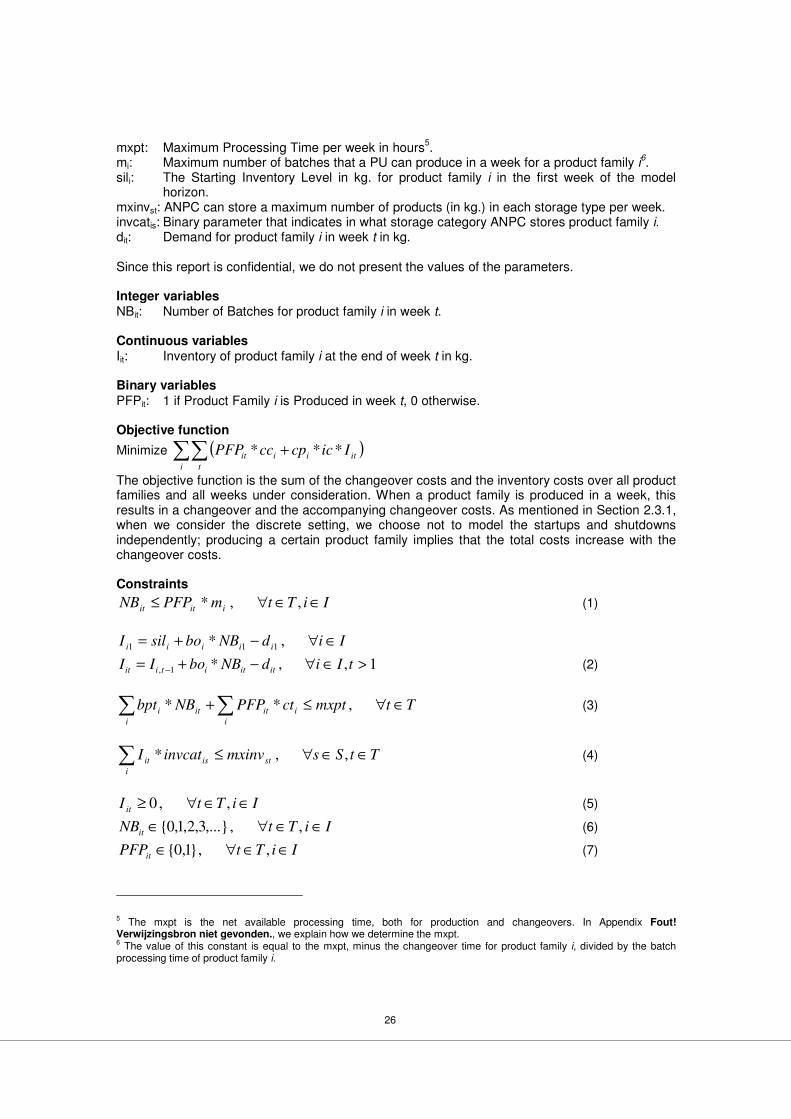
26

mxpt: Maximum Processing Time per week in hours5. mi: Maximum number of batches that a PU can produce in a week for a product family i6. sili: The Starting Inventory Level in kg. for product family i in the first week of the model

horizon. mxinvst: ANPC can store a maximum number of products (in kg.) in each storage type per week. invcatis: Binary parameter that indicates in what storage category ANPC stores product family i. dit: Demand for product family i in week t in kg. Since this report is confidential, we do not present the values of the parameters. Integer variables NBit: Number of Batches for product family i in week t. Continuous variables Iit: Inventory of product family i at the end of week t in kg. Binary variables

PFPit: 1 if Product Family i is Produced in week t, 0 otherwise. Objective function

Minimize ( )∑∑ +i t

itiiit IiccpccPFP ***

The objective function is the sum of the changeover costs and the inventory costs over all product families and all weeks under consideration. When a product family is produced in a week, this results in a changeover and the accompanying changeover costs. As mentioned in Section 2.3.1, when we consider the discrete setting, we choose not to model the startups and shutdowns independently; producing a certain product family implies that the total costs increase with the changeover costs. Constraints

IiTtmPFPNB iitit ∈∈∀≤ ,,* (1)

IidNBbosilI iiiii ∈∀−+= ,*111

1,,*1, >∈∀−+= − tIidNBboII itititiit (2)

∑ ∑ ∈∀≤+i i

iititi TtmxptctPFPNBbpt ,** (3)

TtSsmxinvinvcatIi

stisit ∈∈∀≤∑ ,,* (4)

IiTtI it ∈∈∀≥ ,,0 (5)

IiTtNBit ∈∈∀∈ ,,,...}3,2,1,0{ (6)

IiTtPFPit ∈∈∀∈ ,,}1,0{ (7)

5 The mxpt is the net available processing time, both for production and changeovers. In Appendix Fout! Verwijzingsbron niet gevonden., we explain how we determine the mxpt. 6 The value of this constant is equal to the mxpt, minus the changeover time for product family i, divided by the batch processing time of product family i.

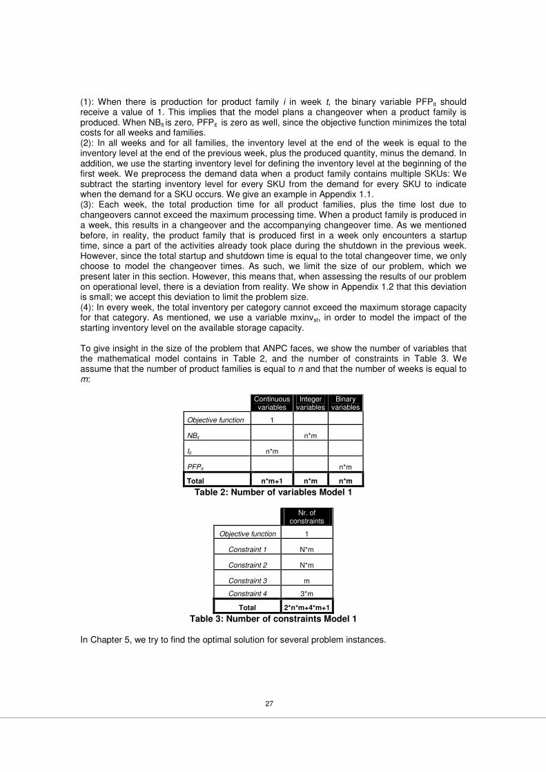
27

(1): When there is production for product family i in week t, the binary variable PFPit should receive a value of 1. This implies that the model plans a changeover when a product family is produced. When NBit is zero, PFPit is zero as well, since the objective function minimizes the total costs for all weeks and families. (2): In all weeks and for all families, the inventory level at the end of the week is equal to the inventory level at the end of the previous week, plus the produced quantity, minus the demand. In addition, we use the starting inventory level for defining the inventory level at the beginning of the first week. We preprocess the demand data when a product family contains multiple SKUs: We subtract the starting inventory level for every SKU from the demand for every SKU to indicate when the demand for a SKU occurs. We give an example in Appendix 1.1. (3): Each week, the total production time for all product families, plus the time lost due to changeovers cannot exceed the maximum processing time. When a product family is produced in a week, this results in a changeover and the accompanying changeover time. As we mentioned before, in reality, the product family that is produced first in a week only encounters a startup time, since a part of the activities already took place during the shutdown in the previous week. However, since the total startup and shutdown time is equal to the total changeover time, we only choose to model the changeover times. As such, we limit the size of our problem, which we present later in this section. However, this means that, when assessing the results of our problem on operational level, there is a deviation from reality. We show in Appendix 1.2 that this deviation is small; we accept this deviation to limit the problem size. (4): In every week, the total inventory per category cannot exceed the maximum storage capacity for that category. As mentioned, we use a variable mxinvst, in order to model the impact of the starting inventory level on the available storage capacity. To give insight in the size of the problem that ANPC faces, we show the number of variables that the mathematical model contains in Table 2, and the number of constraints in Table 3. We assume that the number of product families is equal to n and that the number of weeks is equal to m:

Continuous variables

Integer variables

Binary variables

Objective function 1

NBit n*m

Iit n*m

PFPit n*m

Total n*m+1 n*m n*m

Table 2: Number of variables Model 1

Nr. of

constraints

Objective function 1

Constraint 1 N*m

Constraint 2 N*m

Constraint 3 m

Constraint 4 3*m

Total 2*n*m+4*m+1

Table 3: Number of constraints Model 1

In Chapter 5, we try to find the optimal solution for several problem instances.

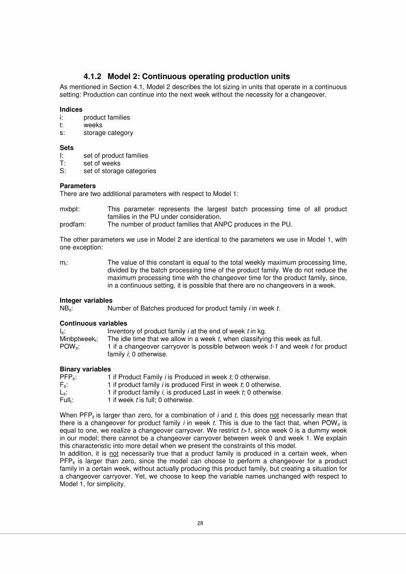
28

4.1.2 Model 2: Continuous operating production units

As mentioned in Section 4.1, Model 2 describes the lot sizing in units that operate in a continuous setting: Production can continue into the next week without the necessity for a changeover. Indices i: product families t: weeks s: storage category Sets I: set of product families T: set of weeks S: set of storage categories Parameters There are two additional parameters with respect to Model 1: mxbpt: This parameter represents the largest batch processing time of all product

families in the PU under consideration. prodfam: The number of product families that ANPC produces in the PU. The other parameters we use in Model 2 are identical to the parameters we use in Model 1, with one exception: mi: The value of this constant is equal to the total weekly maximum processing time,

divided by the batch processing time of the product family. We do not reduce the maximum processing time with the changeover time for the product family, since, in a continuous setting, it is possible that there are no changeovers in a week.

Integer variables NBit: Number of Batches produced for product family i in week t. Continuous variables Iit: Inventory of product family i at the end of week t in kg. Minbptweekt: The idle time that we allow in a week t, when classifying this week as full. POW it: 1 if a changeover carryover is possible between week t-1 and week t for product

family i; 0 otherwise. Binary variables PFPit: 1 if Product Family i is Produced in week t; 0 otherwise. Fit: 1 if product family i is produced First in week t; 0 otherwise. Lit: 1 if product family i, is produced Last in week t; 0 otherwise. Fullt: 1 if week t is full; 0 otherwise. When PFPit is larger than zero, for a combination of i and t, this does not necessarily mean that there is a changeover for product family i in week t. This is due to the fact that, when POW it is equal to one, we realize a changeover carryover. We restrict t>1, since week 0 is a dummy week in our model; there cannot be a changeover carryover between week 0 and week 1. We explain this characteristic into more detail when we present the constraints of this model. In addition, it is not necessarily true that a product family is produced in a certain week, when PFPit is larger than zero, since the model can choose to perform a changeover for a product family in a certain week, without actually producing this product family, but creating a situation for a changeover carryover. Yet, we choose to keep the variable names unchanged with respect to Model 1, for simplicity.

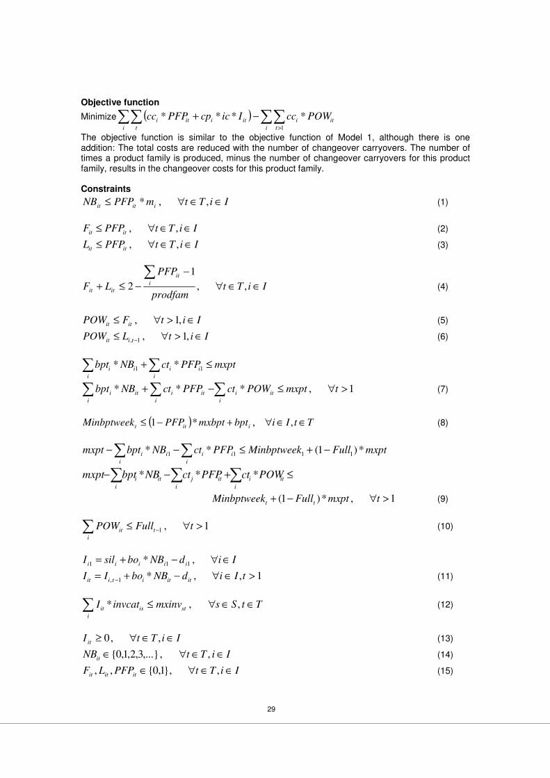
29

Objective function

Minimize ( ) ∑∑∑∑>

−+i t

iti

i t

itiiti POWccIiccpPFPcc1

****

The objective function is similar to the objective function of Model 1, although there is one addition: The total costs are reduced with the number of changeover carryovers. The number of times a product family is produced, minus the number of changeover carryovers for this product family, results in the changeover costs for this product family. Constraints

IiTtmPFPNB iitit ∈∈∀≤ ,,* (1)

IiTtPFPF itit ∈∈∀≤ ,, (2)

IiTtPFPL itit ∈∈∀≤ ,, (3)

IiTtprodfam

PFP

LF i

it

itit ∈∈∀

−

−≤+

∑,,

1

2 (4)

IitFPOW itit ∈>∀≤ ,1, (5)

IitLPOW tiit ∈>∀≤ − ,1,1, (6)

∑ ∑ ≤+i i

iiii mxptPFPctNBbpt11

**

∑ ∑∑ >∀≤−+i i

iti

i

itiiti tmxptPOWctPFPctNBbpt 1,*** (7)

( ) TtIibptmxbptPFPMinbptweek iitt ∈∈∀+−≤ ,,*1 (8)

∑ ∑ −+≤−−i i

iiii mxptFullMinbptweekPFPctNBbptmxpt *)1(**1111

∑ ∑∑ ≤+−−i i

iti

i

itjiti POWctPFPctNBbptmxpt ***

1,*)1( >∀−+ tmxptFullMinbptweek tt (9)

1,1

>∀≤−∑ tFullPOW t

i

it (10)

IidNBbosilI iiiii ∈∀−+= ,*111

1,,*1,

>∈∀−+=−

tIidNBboII itititiit (11)

TtSsmxinvinvcatIi

stisit ∈∈∀≤∑ ,,* (12)

IiTtI it ∈∈∀≥ ,,0 (13)

IiTtNBit ∈∈∀∈ ,,,...}3,2,1,0{ (14)

IiTtPFPLF ititit ∈∈∀∈ ,,}1,0{,, (15)

30

TtFullt ∈∀∈ ,}1,0{ (16)

TtIjiPOWit ∈∈∀≥ ,,,0 (17)

(1): If the models chooses to plan the production for a number of batches for product family i in week t, the binary variable PFPit should receive a value of 1. (2) & (3): The model can only choose to produce a product family i first or last in a week t, when this product family is produced in week t. (4): When there is production for more than one product family in a week, a product family i cannot be produced first and last in this week, due to the necessity for changeovers. For example, it is not possible to define a changeover carryover for a product family for two succeeding weeks, for example between week 1 and week 2, and between week 2 and week 3, when this product family is not the only family that is produced during week 2. (5) & (6): POW it can only be larger than zero when product family i is produced last in week t-1 and first in week t. (7): Each week, the total production time for all product families plus the time lost due to changeovers cannot exceed the maximum available processing time. When a product family is produced in a week, this results in a changeover and the accompanying changeover time. For week 1, there cannot be a correction for possible changeover carryovers with the previous week, since week 1 represents the first week in the model. For the remaining weeks, when the first product family produced in week t is identical to the last product family produced in week t-1, we exclude the accompanying changeover time from the changeover downtime, in week t. (8): A changeover can only be preserved between two weeks, when there is limited idle time in the preceding week; when the preceding week is full. The reason is that, when the preceding week is not full, there is a shutdown before the end of the week, due to safety issues: Operators need to clean the reactor and possibly change the setup of the PU. When there was a shutdown in the preceding week, there can be no changeover carryover, since production cannot continue in the next week without the necessity for a changeover in the PU. For example, after the shutdown, operators need to setup the PU and prepare the reactor for the chemical reaction. When PFPit, for a product family i in a week t is larger than zero, the model has the possibility to plan a batch for the accompanying batch processing time (bpti). As a result, the idle time that we allow in week t is restricted to the lowest bpti of the product families that are produced in this week. After all, more idle time indicates that additional batches could be planned; the week is not full. When PFPit, for a product family i in a week t, is equal to zero, we do not restrict the idle time to be lower than the accompanying bpti. In other words, when the remaining capacity is smaller than the Minbptweekt, it is not possible to add a batch of a product family that is planned in that week; the week is full. (9): When the remaining production capacity in week t is smaller than the Minbptweekt, the variable Fullt can obtain a value of 1. (10): By restricting the sum of POW it over all product families to be smaller than Fullt-1, we ensure there can only be a changeover carryover in week t, when week t-1 is full. (11): In all weeks and for all families, the inventory level at the end of the week is equal to the inventory level at the end of the previous week, plus the production quantity, minus the demand. (12): In every week, total inventory per category cannot exceed the maximum storage capacity for that category. (17): We do not restrict POW it to be binary, in order to reduce the number of binary variables in the model. We expect that the presence of the objective function ensures that POW it will be no less than one, when POW it is allowed to be one. However, the situation could arise in which the model chooses POW it to be fractional, when this implies that a week t becomes Full (constraint 9). When we encounter this situation when solving the model for a problem instance, we restrict POW it to be binary. However, initially, we choose POW it to be continuous. Again, we give insight in the size of the problem that ANPC faces: We present the number of variables that the mathematical model contains in Table 4, and the number of constraints in Table 5. We assume that the number of product families is equal to n and that the number of weeks is equal to m:

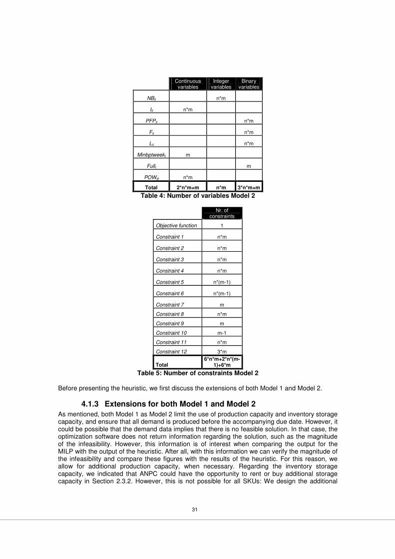
31

Continuous variables

Integer variables

Binary variables

NBit n*m

Iit n*m

PFPit n*m

Fit n*m

Lit n*m

Minbptweekt m

Fullt m

POWijt n*m

Total 2*n*m+m n*m 3*n*m+m

Table 4: Number of variables Model 2

Nr. of

constraints

Objective function 1

Constraint 1 n*m

Constraint 2 n*m

Constraint 3 n*m

Constraint 4 n*m

Constraint 5 n*(m-1)

Constraint 6 n*(m-1)

Constraint 7 m

Constraint 8 n*m

Constraint 9 m

Constraint 10 m-1

Constraint 11 n*m

Constraint 12 3*m

Total 6*n*m+2*n*(m-

1)+6*m

Table 5: Number of constraints Model 2 Before presenting the heuristic, we first discuss the extensions of both Model 1 and Model 2.

4.1.3 Extensions for both Model 1 and Model 2

As mentioned, both Model 1 as Model 2 limit the use of production capacity and inventory storage capacity, and ensure that all demand is produced before the accompanying due date. However, it could be possible that the demand data implies that there is no feasible solution. In that case, the optimization software does not return information regarding the solution, such as the magnitude of the infeasibility. However, this information is of interest when comparing the output for the MILP with the output of the heuristic. After all, with this information we can verify the magnitude of the infeasibility and compare these figures with the results of the heuristic. For this reason, we allow for additional production capacity, when necessary. Regarding the inventory storage capacity, we indicated that ANPC could have the opportunity to rent or buy additional storage capacity in Section 2.3.2. However, this is not possible for all SKUs: We design the additional

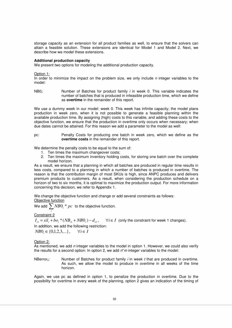
32

storage capacity as an extension for all product families as well, to ensure that the solvers can attain a feasible solution. These extensions are identical for Model 1 and Model 2. Next, we describe how we model these extensions. Additional production capacity We present two options for modeling the additional production capacity. Option 1: In order to minimize the impact on the problem size, we only include n integer variables to the model: NB0i: Number of Batches for product family i in week 0. This variable indicates the

number of batches that is produced in infeasible production time, which we define as overtime in the remainder of this report.

We use a dummy week in our model: week 0. This week has infinite capacity; the model plans production in week zero, when it is not possible to generate a feasible planning within the available production time. By assigning (high) costs to this variable, and adding these costs to the objective function, we ensure that the production in overtime only occurs when necessary; when due dates cannot be attained. For this reason we add a parameter to the model as well: pc: Penalty Costs for producing one batch in week zero, which we define as the

overtime costs in the remainder of this report. We determine the penalty costs to be equal to the sum of:

1. Ten times the maximum changeover costs; 2. Ten times the maximum inventory holding costs, for storing one batch over the complete

model horizon. As a result, we ensure that a planning in which all batches are produced in regular time results in less costs, compared to a planning in which a number of batches is produced in overtime. The reason is that the contribution margin of most SKUs is high, since ANPC produces and delivers premium products to customers. As a result, when considering the production schedule on a horizon of two to six months, it is optimal to maximize the production output. For more information concerning this decision, we refer to Appendix 1. We change the objective function and change or add several constraints as follows: Objective function

We add ∑i

i pcNB *0 to the objective function.

Constraint 2

IidNBNBbosilI iiiiii ∈∀−++= ,)0(*111

(only the constraint for week 1 changes).

In addition, we add the following restriction:

IiNB i ∈∀∈ ,,...}3,2,1,0{0

Option 2: As mentioned, we add n integer variables to the model in option 1. However, we could also verify the results for a second option: In option 2, we add n*m integer variables to the model: NBerrorit: Number of Batches for product family i in week t that are produced in overtime.

As such, we allow the model to produce in overtime in all weeks of the time horizon.

Again, we use pc as defined in option 1, to penalize the production in overtime. Due to the possibility for overtime in every week of the planning, option 2 gives an indication of the timing of

33

the overtime (what weeks are highly utilized). Nevertheless, the number of (integer) variables increases with n*m, instead of only with n. We change the objective function and change or add several constraints as follows: Objective function

We add ∑∑i t

it pcNBerror * to the objective function.

Constraint 2

IidNBerrorNBbosilI iiiiii ∈∀−++= ,)(*1111

1,,)(*1, >∈∀−++= − tIidNBerrorNBboII ititititiit

In addition, we add the following restriction:

IiTtNBerrorit ∈∈∀∈ ,,,...}3,2,1,0{

To conclude, we determine the additional required batch processing time; we do not determine the additional required changeover time. When necessary, we can calculate the number of additional required changeovers from the output by determining the number of weeks in which a certain product family is produced in overtime, while this product family is not produced in regular time. Additional inventory storage capacity

We include 3*m continuous variables in the model: InvErrorts: The increase of the inventory above the maximum storage capacity in week t in

storage category s in kg. When it is not possible to use additional storage capacity, we need to assign penalty costs for increasing the inventory level above the storage capacity: We need to ensure that the inventory level is only increased above the capacity limit when necessary; when due dates cannot be attained. Naturally, when increasing the IPC above the overtime costs, the priority of reducing the additional inventory storage outweighs the priority for reducing the overtime. We add the following parameter to the model: ipcs: Inventory costs for increasing the inventory level above the available storage

capacity for category s in €/kg. We define these costs as the Inventory Penalty Costs (IPC) in the remainder of this report.

In our research, we allow the inventory level per category to increase above the maximum storage capacity per category, without penalizing this violation. In other words, the IPC are equal to zero for every storage category s. The reason is that there is no univocal rule within the logistical department that defines the maximum storage capacity per storage category per PU (mxinvst), since this amount depends on the varying inventory levels of the product families that are produced in the other Pus on the site. In other words, several PUs utilize the storage capacity and there is no allocation rule, yet. Concluding, we could exclude the storage capacity constraints and this extension from Model 1, such that we decrease the problem size. However, we include the constraints and this extension, in order to test the output of the solvers for the complete problem. We change the objective function and change or add several constraints as follows: Objective function

We add ∑∑t s

sts ipcInvError * to the objective function.

34

Constraint 4

TtSsInvErrormxinvinvcatI ts

i

sisit ∈∈∀+≤∑ ,,*

In addition, we add the following restriction:

SsTtInvErrorts ∈∈∀≥ ,,0

4.2 Developing a lot sizing heuristic As mentioned in Section 3.5, we develop a period-by-period heuristic and a SA algorithm. We discuss the period-by-period heuristic in Section 4.2.1. Next, we discuss the SA algorithm in Section 4.2.2. However, first, we recapitulate on our assumptions and findings from earlier chapters:

1. The problem characteristics are identical to the characteristics that we mention in Section 4.1.

2. We develop two versions of the SA algorithm: The first version is applicable to PUs that operate in a discrete setting, the second to PUs that operate in a continuous setting.

3. In comparison with the MILPs, the planning can contain production in overtime and inventory levels that are higher than the defined maximum inventory storage capacity per category.

4. In Chapter 5, we verify the results and test the SA algorithm in combination with the period-by-period heuristic; we use the output of the period-by-period heuristic as a starting solution for the SA algorithm. In addition, we verify the results when using another starting solution, and using different NSs in the SA algorithm.

4.2.1 Period-by-period heuristic

We first discuss the outline of the period-by-period heuristic, after which we present the steps of this heuristic into more detail.

4.2.1.1 Outline

In accordance with Chapter 3, we base the period-by-period heuristic on the DS heuristic. However, there are some deviations with respect to the DS heuristic, since this heuristic does not consider the inclusion of changeover times. We discuss these deviations subsequently, but first we present the similarities, which actually comprise the three general steps of the heuristic:

1. We generate an initial planning based on the lot-for-lot rule. As a result, in the initial planning, the accompanying inventory levels are zero.

2. We reallocate runs in order to create a feasible production planning. 3. Identify, after reallocating runs, possibilities for combining runs.

In contrast with the problem that the DS heuristic considers, we face a problem that includes changeover times and an inventory constraint. The implications for our heuristic are that:

1. We reallocate runs by starting in the last week of the horizon, and proceed backwardly. The reason is that, when considering the last week of the horizon, it is only possible to produce the forecasted demand that belongs to this last week. After all, producing the forecasted demand of earlier weeks means that the planning disrespects due dates. When the requirements in the last week imply the use of overtime, it is necessary to reallocate (a part of the) runs. Consequently, all information on which to base the decision for reallocating forecasted demand is known, when proceeding backwardly. In contrast, when starting in the first week of the planning, we cannot decide on a reallocation, since this depends on the unidentified amount of changeover time in the subsequent weeks. Concluding, we deviate from the DS heuristic with respect to reallocating runs, since the DS heuristic does not consider changeover times and can decide on reallocating runs by starting in the first week.

2. We choose a family-by-family approach. As such, we introduce a product family to the planning, and evaluate possibilities for reallocating and combining runs, before adding

35

another product family to the planning. When we do not take a family-by-family approach, the lot-for-lot rule would imply that the initial planning can contain an abundance of changeovers. As such, production is reallocated via the backward approach that we discussed before. After this reallocation step, week one contains overtime, while the other weeks contain short idle time. As such, it is not possible to combine runs and create a good starting solution.

3. We presented the rules for reallocating and combining runs from the DS heuristic and the SM heuristic in Section 3.4.2: The rule with which we determine how to reallocate and combine runs is based on the SM heuristic. Naturally, we do take the capacity impact into account when combining runs.

4. When reallocating or combining production runs, the situation can arise in which the inventory level increases above the inventory storage capacity limit. We attempt to reduce possible storage capacity violations via the use of the SA algorithm.

5. Since we consider the problem family-by-family, we need to decide on a priority rule for introducing product families to the planning. We evaluate two options for introducing product families to the planning: a) Kirca and Kökten (1992) performed several test regarding how to introduce items to

the planning. They conclude that the following approach outperforms others: They

calculate the average costs per item i as follows:i

iii

d

dcpiccc ****2, in which:

1. cci represents the changeover costs for item i. 2. ic represents the inventory costs (as a percentage of the inventory value). 3. cpi represents the cost price for item i.

4. −

id represents the total demand for item i over all periods that are considered.

The item with the largest average costs per item is considered for scheduling first. We define this priority rule as the KK rule.

b) Gupta and Magnusson (2005) introduce items to the planning in the order of decreasing cumulative demand. They argue that by scheduling the high volume products first, it is easier to generate a planning, since the remaining gaps can be filled by planning the products with a low cumulative demand. We define their priority rule as the GM rule. The GM rule contradicts with the KK rule. After all, by applying the KK rule, items with a relative low average demand receive a higher priority, with respect to items with a high average demand. We test to what extent this affects the quality of the starting solution.

Summarizing, the heuristic functions as follows, family-by-family:

1. Generate an initial planning for a product family via the lot-for-lot rule. 2. Construct a feasible planning by reallocating batches via evaluating the periods

backwardly. 3. Consider improvement opportunities via the SM heuristic within the bounds of feasibility.

We repeat the process until we considered all product families. Before we discuss above steps into more detail, we make two remarks:

1. After introducing all product families to the planning, the situation could arise in which the heuristic cannot find a feasible planning: The remaining production capacity and the remaining inventory storage capacity could be negative in one or more weeks. Still, these possible capacity violations can be reduced when considering improvement opportunities via running the SA algorithm after the period-by-period heuristic.

2. We test a third starting solution. In this starting solution, the demand of the fist half of the horizon is produced in the first week, and the remaining demand in the middle week. We define this starting solution as ½T. By applying this third starting solution, we can assess the impact of the quality of the starting solution on the output. We could also choose to test the impact of starting solutions in which all demand is produced in one, three, four, or

36

more weeks. Yet, we do not have the time to test the impact of all these different starting solutions. In addition, we expect that verifying three starting solutions already gives a good indication regarding the impact on the output.

Concluding, we test three different starting solutions in our research: 1. Starting solution 1: Family-by-family approach based on the KK rule and reallocating and

combining runs based on the SM heuristic. 2. Starting solution 2: Family-by-family approach based on the GM rule and reallocating and

combining runs based on the SM heuristic. 3. Starting solution 3: Producing the demand of the first half of the horizon in the first week,

and the remaining demand in the middle week.

4.2.1.2 Steps

In order to elaborate upon the steps that underlie the period-by-period heuristic, we first introduce several definitions:

1. The definitions for the indices, sets, parameters, and variables are similar to the definitions we use for the mathematical models.

2. We define n to represent the total number of product families under consideration. 3. We use the term maxt to refer to the last week in the horizon.

Step 1: Sort all product families

In case of the KK rule: The priority is based on the largest average costs per product family:

i

iii

id

dcpicccAC

****2= . The product family with the highest priority, receives index one.

In case of GM rule: The priority is based on the Total Demand (TDi) per product family over all weeks:

∑ ∈∀=t

iti IidTD , .

We perform step 2 until step 6 of the heuristic family-by-family, starting with the product family with the first index, and concluding with the family with the index that is equal to n. Step 2: Generate production runs based on the lot-for-lot rule

The heuristic generates a production run for every week that there exists forecasted demand.

Consequently,i

it

itbo

dNB = . The outcome of the equation could be fractional; the next step

ensures that all runs contain an integer number of batches. Step 3: Ensure that all runs contain an integer number of batches

We round the number of batches in a run upwards to the nearest integer. This implies that the run does not only satisfy the demand for one period, but rather is building up (a minor amount of) inventory, which we define as the additional inventory. In order to minimize this additional inventory, we correct NBit: When the sum the additional inventory is larger than one batch, we decrease NBit with one in the subsequent week. For example, when the additional inventory in the first three weeks is larger than one batch, we decrease NBit with one in week four. Step 4: Calculate the remaining production cap. and inventory storage cap. per week We calculate the remaining production capacity (RC) per week as follows:

( ) TtNBbptctPFPmxptRCi

itiiitt ∈∀+−= ∑ ,** .

We calculate the remaining inventory storage capacity per category per week as follows:

SsTtinvcatImxinvRIi

isitstts ∈∈∀−= ∑ ,,* .

37

In which we determine the inventory level via:

IidNBbosilI iiiii ∈∀−+= ,*111

1,,*1,

>∈∀−+=−

tIidNBboII itititiit

Step 5: Reallocate production runs In this step of the heuristic we evaluate whether we need to reallocate runs. We proceed backwardly, from week maxt until week 2, since we cannot reallocate runs that reside in week 1. When we encounter a period in which the remaining production capacity is negative, we calculate the amount with which the production should decline in order to increase the remaining production capacity above zero. As indicated in Section 4.2.1.1, we attempt to reduce possible storage capacity violations via the use of the SA algorithm.

Step 6: Improve the feasible planning In this step of the heuristic we verify whether we can combine two production runs of the same product family. We base the criterion for combining runs on the SM heuristic. We proceed forwardly, from week 1 until week maxt. Next, we discuss the SA algorithm.

4.2.2 Simulated annealing

First, we present the outline. Next, we discuss the steps in more detail.

4.2.2.1 Outline

According to Tang (2004), when developing a SA algorithm, we need to decide on how to generate NSs and how to define the Cooling schedule. Following, we discuss these two decisions. Neighbourhood solutions Kuik and Salomon (1990), Meyr (2000), and Tang (2004), who discuss the implementation of the SA algorithm in different lot sizing problems, define NSs by randomly selecting a feasible change in the changeover pattern: Creating, deleting, or exchanging runs of an existing solution in order to create a feasible NS. In addition, Özdamar and Bozyel (1999) exchange a random amount between two runs of the same product family and indicate that this supports their goal of transitioning production from a bottleneck period to a non-bottleneck period, in order to lower the total costs. They define a bottleneck period as a period in which it is not possible to produce all forecasted demand that resides in that period. For above reasons, our SA algorithm evaluates whether there are opportunities for exchanging a (part of) a run to another week. We define this as rearranging runs. We test two options:

1. Rearranging runs between two randomly chosen succeeding weeks (NS1). 2. Rearranging runs between two randomly chosen weeks (NS2).

Cooling schedule According to Tang (2004), the cooling schedule has a large impact on the functioning of the SA algorithm. Determining the cooling schedule means that we have to decide on the values for:

1. The starting temperature; 2. The cooling parameter (CP); 3. Iter: how many NSs we evaluate before lowering the Temperature with the CP; 4. The stopping criterion.

As mentioned in Section 3.4.2, NSs that deteriorate the objective function are accepted against a certain probability: the Probability of Acceptance (PA). By deciding on the value for starting temperature, we implicitly decide on the PA. In accordance with Kirkpatrick et al. (1983) we choose the PA to be equal to: exp(-costdifference/temperature), with:

1. Costdifference: The cost difference between the NS and the current planning.

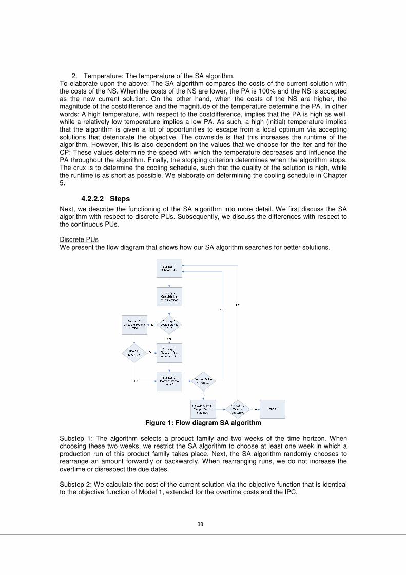
38

2. Temperature: The temperature of the SA algorithm. To elaborate upon the above: The SA algorithm compares the costs of the current solution with the costs of the NS. When the costs of the NS are lower, the PA is 100% and the NS is accepted as the new current solution. On the other hand, when the costs of the NS are higher, the magnitude of the costdifference and the magnitude of the temperature determine the PA. In other words: A high temperature, with respect to the costdifference, implies that the PA is high as well, while a relatively low temperature implies a low PA. As such, a high (initial) temperature implies that the algorithm is given a lot of opportunities to escape from a local optimum via accepting solutions that deteriorate the objective. The downside is that this increases the runtime of the algorithm. However, this is also dependent on the values that we choose for the Iter and for the CP: These values determine the speed with which the temperature decreases and influence the PA throughout the algorithm. Finally, the stopping criterion determines when the algorithm stops. The crux is to determine the cooling schedule, such that the quality of the solution is high, while the runtime is as short as possible. We elaborate on determining the cooling schedule in Chapter 5.

4.2.2.2 Steps

Next, we describe the functioning of the SA algorithm into more detail. We first discuss the SA algorithm with respect to discrete PUs. Subsequently, we discuss the differences with respect to the continuous PUs. Discrete PUs We present the flow diagram that shows how our SA algorithm searches for better solutions.

Figure 1: Flow diagram SA algorithm

Substep 1: The algorithm selects a product family and two weeks of the time horizon. When choosing these two weeks, we restrict the SA algorithm to choose at least one week in which a production run of this product family takes place. Next, the SA algorithm randomly chooses to rearrange an amount forwardly or backwardly. When rearranging runs, we do not increase the overtime or disrespect the due dates. Substep 2: We calculate the cost of the current solution via the objective function that is identical to the objective function of Model 1, extended for the overtime costs and the IPC.

39

Substep 5: PA is the value for the probability of acceptance, which we mentioned in Section 4.2.2.1. Rand represents a random number between 0 and 1. Substep 7-10: After analyzing a NS, the SA algorithm increases the number of iterations with one. When the number of iterations reaches Iter, the temperature is lowered with the CP. This process repeats itself until the temperature reaches the stopping temperature. Above process does not change when using another starting solution or choosing NSs differently. Only the content of substep one changes by choosing the two weeks differently. Continuous PUs Until now, we did not discuss the inclusion of changeover carryovers. Yet, it is possible to preserve a changeover in PUs that operate in a continuous setting. As such, before starting the SA algorithm, the heuristic evaluates whether the PP contains two production runs for the same product family in two consecutive weeks, in order to analyze whether there are carryover possibilities. We start this evaluation in week two, and consider the production runs in this week and the previous week. Naturally, changeover carryovers are only possible when the preceding week is full; when the remaining capacity is lower than the Minbptweek. When there are several product families that are produced in both weeks, the heuristic chooses the carryover that implies the highest cost saving. Actually, we assume that this product family is produced first in week two, and last in week one. The changeover is removed from the week with the highest index, in this case week two. Then, we proceed to the next week, and consider the production runs in week three and week two, etc. Naturally, we take into account that, when there already is a carryover between week t-1 and week t-2 for product family i, we can only define a changeover carryover for this family, when this family is the only family that is produced in week t-1. To summarize, before we start the SA algorithm, we evaluate in which weeks we generate a changeover carryover: We verify for every week whether the preceding week is full, and whether there are product families that are produced in week t as well as week t-1. If yes, we choose the changeover carryover that results into the largest savings. Next, we start the SA algorithm in which we take into account that a NS can contain an additional changeover carryover. When this leads to a NS with lower costs, the SA algorithm chooses this NS as the new current solution. Concluding, the SA algorithm is comparable for PUs that operate in a discrete and a continuous setting. There are two differences:

1. When defining the Costdifference, the SA algorithm takes the additional costs, or additional savings, due to deleting or creating changeover carryovers into account.

2. When deleting a changeover carryover from a week due to a rearrangement, we verify whether we could preserve this carryover or ensure that there is a possibility for another carryover. We explain this process via an example: Assume we rearrange a run from week 1 to week 4 for product family 1 (Fam1). Due to the rearrangement, the carryover between week 1 and week 2 is deleted, since week 1 is not full anymore. For this reason, we verify whether we can increase the production in week 1 for Fam1, by rearranging production from week 2 to week 1. When we can eliminate the idle time in week 1, we could preserve the carryover, or ensure a possibility for another carryover. As such, we assess two rearrangements in one NS. Of course, it is also possible to create changeover carryovers by verifying the NSs.

To conclude: We developed two MILPs that describe the lot sizing problem that ANPC faces in both discrete and continuous PUs. In addition, we developed a hybrid heuristic that consist of a period-by-period heuristic, which calculates a starting solution, and a SA algorithm that iteratively searches for improvements. By developing three different starting solutions and two ways of searching for NSs, we developed six different heuristics. In order to verify the quality of the different heuristics, we compare the results of solving the MILPs via optimization software with the results of the heuristics in Chapter 5.

40

Chapter 5 Results & Implications In this chapter, we present the results of solving the mathematical models, which we developed in Chapter 4, via optimization software and calculate the results by using the six heuristics. In addition, we assess the current situation and discuss the implications of applying the results in practice. In Section 5.1, we first present the framework on which we base our tests. In Section 5.2, we assess the results of solving the mathematical models via optimization software. In Section 5.3, we assess the results of the heuristics and make a comparison with the results from Section 5.2. In Section 5.4, we compare the results of the heuristics with the current performance and the current policy, which we presented in Chapter 2. Finally, in Section 5.5, we discuss the implications of applying the results in practice.

5.1 Framework In this section, we first present the problem instances that we consider in Section 5.1.1. Next, we elaborate on the optimization software that we use in Section 5.1.2 and review the heuristics that we test in Section 5.1.3. Finally, we discuss how we asses the results in Section 5.1.4.

5.1.1 Problem instances

As presented in Section 2.3, we consider the lot sizing in four distinct PUs. For every PU, we acquired the demand data for the last 26 weeks of 2009. As mentioned in Section 4.1.1, we excluded the input data from this report. When we would use the acquired demand data to perform our tests, we test four different problem instances. In order to increase the number of problem instances that we test, we adapted the demand data, such that we realize three different utilization levels in every PU:

1. 65%: The lowest utilization level we encountered in the four PUs under consideration is 65%: At the end of 2008 and the beginning of 2009 the utilization was low, due to the credit crunch.

2. 100%: The highest utilization level we test is 100%, although Hopp and Spearman (2001) indicate that it is impossible to attain a utilization level of 100% in practice, due to the variability in the production process. The reason that we still test the PUs for this utilization level is that we want to assess the results of the optimization software and the heuristics when the utilization level implies that we can expect that overtime is insurmountable.

3. 82.5%: We also verify the results for a moderate utilization level: 82.5%; the average of 65% and 100%.

We adapt the demand data as follows: 1. Since the utilization level depends on the changeover time, which we cannot determine

on beforehand, we assume that the changeover time is equal to the average historic changeover time per PU.

2. Subsequently, we adapt the demand data by multiplying the demand in every week for every product family with the same factor in order to realize the target utilization level. We define the resulting problem instances as problems with respectively a low, medium, or high demand.

As we mentioned in Section 4.1.1, we take the starting inventory level into account when defining the demand. Concluding, we consider twelve different problem instances: Three problem instances per PU.

5.1.2 Optimization software

In Section 4.1, we developed two mathematical models in order to assess the results of the heuristics:

1. Model 1: Applicable to PUs that operate in a discrete setting. 2. Model 2: Applicable to PUs that operate in a continuous setting.

41

For each model, we developed two extensions that allow for overtime, which we define as Option 1 (O1) and Option 2 (O2). We only calculate the results for Model 1 and 2 extended for O1, since this extension is based on the same assumptions as the heuristics: Overtime is only allowed in the beginning of the time horizon. In O1, we use a dummy week; week zero. For the heuristics, we allow overtime in week 1 of the time horizon. This implies that we measure the inventory costs identically, since we measure the inventory level at the end of week 1; we do not include the inventory costs of week zero. Next to the overtime, we allow for additional inventory storage capacity, as indicated in Section 4.1.3. We are able to use two types of optimization software, or solvers:

1. CPLEX 10 (CPLEX), available via a license of the University of Twente. 2. GAMS/XPRESS (G/X), freely available via the Network-Enabled Optimization System

(NEOS) server. Both solvers are qualified as high-performance solvers: (http://www.gams.com/solvers/index.html). For this reason, we choose to use both solvers in our research. We run CPLEX on an Intel Pentium M 1.73GHz processor. In contrast, we do not have information concerning the capacity of the NEOS server: We only know that the NEOS sever has an automatic timeout of 48 hours for problems that contain integer variables. In addition, we cannot submit a problem that is larger than 16.8 MB. We present more information concerning both solvers in Appendix 3, including more information concerning the branch-and-bound process.

5.1.3 Heuristics

As presented in Section 4.1.3, we develop three different starting solutions for the SA algorithm and two methods by which the SA algorithm searches for NSs, which we define as a NS-method. We review these starting solutions and NS-methods: Starting solution 1: Family-by-family approach based on the KK rule and reallocating and combining runs based on the SM heuristic. Starting solution 2: Family-by-family approach based on the GM rule and reallocating and combining runs based on the SM heuristic. Starting solution 3: Producing the demand of the fist half of the horizon in the first week, and the remaining demand in the middle week. NS-method 1: Rearranging runs between two randomly chosen succeeding weeks. NS-method 2: Rearranging runs between two randomly chosen weeks. As such, we test all problem instances for six different heuristics, which we define as follows:

1. KK-NS1: Starting solution 1 and NS-method 1. 2. GM-NS1: Starting solution 2 and NS-method 1. 3. ½T-NS1: Starting solution 3 and NS-method 1. 4. KK-NS2: Starting solution 1 and NS-method 2. 5. GM-NS2: Starting solution 2 and NS-method 2. 6. ½T-NS2: Starting solution 3 and NS-method 2.

Of course, when testing the heuristics for PUs that operate in a continuous setting, we allow the SA algorithm to define changeover carryovers. For all heuristics, we present the results of running the SA algorithm for an identical cooling schedule. As we discussed in Section 4.2.2.1, we need to decide on the values for the following parameters:

1. The starting temperature; 2. The CP; 3. Iter: how many NSs we evaluate before lowering the Temperature with the CP; 4. The stopping criterion.

The choice for the parameters of the cooling schedule has a large impact on the functioning of the SA algorithm, as Tang (2004) indicates. In addition, according to Kim et al. (2002), the characteristics of the problem influence the decision for the cooling schedule. Furthermore, Tang

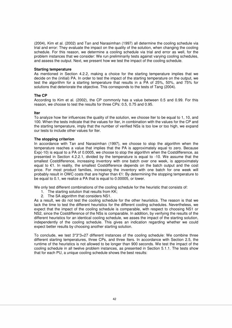
42

(2004), Kim et al. (2002) and Tan and Narasimhan (1997) all determine the cooling schedule via trial and error: They evaluate the impact on the quality of the solution, when changing the cooling schedule. For this reason, we determine a cooling schedule via trial and error as well, for the problem instances that we consider: We run preliminarily tests against varying cooling schedules, and assess the output. Next, we present how we test the impact of the cooling schedule. Starting temperature As mentioned in Section 4.2.2, making a choice for the starting temperature implies that we decide on the (initial) PA. In order to test the impact of the starting temperature on the output, we test the algorithm for a starting temperature that results in a PA of 25%, 50%, and 75% for solutions that deteriorate the objective. This corresponds to the tests of Tang (2004). The CP

According to Kim et al. (2002), the CP commonly has a value between 0.5 and 0.99. For this reason, we choose to test the results for three CPs: 0.5, 0.75 and 0.95. Iter

To analyze how Iter influences the quality of the solution, we choose Iter to be equal to 1, 10, and 100. When the tests indicate that the values for Iter, in combination with the values for the CP and the starting temperature, imply that the number of verified NSs is too low or too high, we expand our tests to include other values for Iter. The stopping criterion In accordance with Tan and Narasimhan (1997), we choose to stop the algorithm when the temperature reaches a value that implies that the PA is approximately equal to zero. Because Exp(-10) is equal to a PA of 0.0005, we choose to stop the algorithm when the Costdifference, as presented in Section 4.2.2.1, divided by the temperature is equal to -10. We assume that the smallest Costdifference, increasing inventory with one batch over one week, is approximately equal to €1. In reality, the smallest Costdifference depends on the batch output and the cost price. For most product families, increasing the inventory with one batch for one week will probably result in OWC costs that are higher than €1: By determining the stopping temperature to be equal to 0.1, we realize a PA that is equal to 0.00005, or lower. We only test different combinations of the cooling schedule for the heuristic that consists of:

1. The starting solution that results from KK; 2. The SA algorithm that considers NS1.

As a result, we do not test the cooling schedule for the other heuristics. The reason is that we lack the time to test the different heuristics for the different cooling schedules. Nevertheless, we expect that the impact of the cooling schedule is comparable, with respect to choosing NS1 or NS2, since the Costdifference of the NSs is comparable. In addition, by verifying the results of the different heuristics for an identical cooling schedule, we asses the impact of the starting solution, independently of the cooling schedule. This gives an indication regarding whether we could expect better results by choosing another starting solution. To conclude, we test 3*3*3=27 different instances of the cooling schedule: We combine three different starting temperatures, three CPs, and three Iters. In accordance with Section 2.5, the runtime of the heuristics is not allowed to be longer than 900 seconds. We test the impact of the cooling schedule in all twelve problem instances, as presented in Section 5.1.1. The tests show that for each PU, a unique cooling schedule shows the best results:

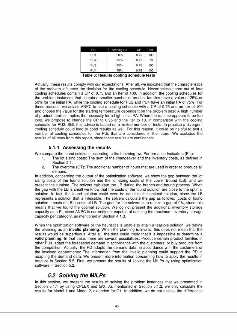
43

PU Starting PA CP Iter

PU1 50% 0.75 100

PU2 75% 0.95 10

PU3 25% 0.75 100

PU4 75% 0.75 100

Table 6: Results cooling schedule tests Actually, these results comply with our expectations. After all, we indicated that the characteristics of the problem influence the decision for the cooling schedule. Nevertheless, three out of four cooling schedules contain a CP of 0.75 and an Iter of 100. In addition, the cooling schedules for the problem instances that contain a smaller number of product families have a value of 25% or 50% for the initial PA, while the cooling schedule for PU2 and PU4 have an initial PA of 75%. For these reasons, we advise ANPC to use a cooling schedule with a CP of 0.75 and an Iter of 100 and choose the value for the starting temperature dependent on the problem size: A high number of product families implies the necessity for a high initial PA. When the runtime appears to be too long, we propose to change the CP to 0.95 and the Iter to 10, in comparison with the cooling schedule for PU2. Still, this advice is based on a limited number of tests: In practice a divergent cooling schedule could lead to good results as well. For this reason, it could be helpful to test a number of cooling schedules for the PUs that are considered in the future. We excluded the results of all tests from this report, since these results are confidential.

5.1.4 Assessing the results

We compare the found solutions according to the following two Performance Indicators (PIs): 1. The lot sizing costs: The sum of the changeover and the inventory costs, as defined in

Section 2.1. 2. The overtime (OT): The additional number of hours that are used in order to produce all

demand. In addition, concerning the output of the optimization software, we show the gap between the lot sizing costs of the found solution and the lot sizing costs of the Lower Bound (LB), and we present the runtime. The solvers calculate the LB during the branch-and-bound process. When the gap with the LB is small we know that the costs of the found solution are close to the optimal solution. In fact, the found solution could even be equal to the optimal solution, since the LB represents a solution that is infeasible. The solvers calculate the gap as follows: (costs of found solution – costs of LB) / costs of LB. The goal for the solvers is to realize a gap of 0%, since this means that we found the optimal solution. We do not present the additional inventory storage capacity as a PI, since ANPC is currently not capable of defining the maximum inventory storage capacity per category, as mentioned in Section 4.1.3. When the optimization software or the heuristics is unable to attain a feasible solution, we define the planning as an invalid planning. When the planning is invalid, this does not mean that the results would be superfluous. After all, the data could imply that it is impossible to determine a valid planning. In that case, there are several possibilities: Produce certain product families in other PUs, adapt the forecasted demand in accordance with the customers, or buy products from the competition. Actually, the PD adapts the demand data, in accordance with the customers or the involved departments: The information from the invalid planning could support the PD in adapting the demand data. We present more information concerning how to apply the results in practice in Section 5.5. First, we present the results of solving the MILPs by using optimization software in Section 5.2.

5.2 Solving the MILPs In this section, we present the results of solving the problem instances that we presented in Section 5.1.1 by using CPLEX and G/X. As mentioned in Section 5.1.2, we only calculate the results for Model 1 and Model 2, extended for O1. In addition, we do not assess the differences

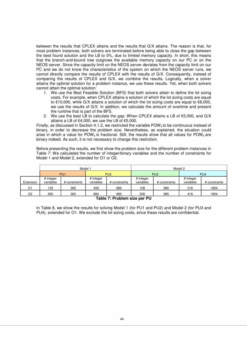
44

between the results that CPLEX attains and the results that G/X attains. The reason is that, for most problem instances, both solvers are terminated before being able to close the gap between the best found solution and the LB to 0%, due to limited memory capacity. In short, this means that the branch-and-bound tree outgrows the available memory capacity on our PC or on the NEOS server. Since the capacity limit on the NEOS server deviates from the capacity limit on our PC and we do not know the characteristics of the system on which the NEOS server runs, we cannot directly compare the results of CPLEX with the results of G/X. Consequently, instead of comparing the results of CPLEX and G/X, we combine the results. Logically, when a solver attains the optimal solution for a problem instance, we use these results. Yet, when both solvers cannot attain the optimal solution:

1. We use the Best Feasible Solution (BFS) that both solvers attain to define the lot sizing costs. For example, when CPLEX attains a solution of which the lot sizing costs are equal to €10,000, while G/X attains a solution of which the lot sizing costs are equal to €8,000, we use the results of G/X. In addition, we calculate the amount of overtime and present the runtime that is part of the BFS.

2. We use the best LB to calculate the gap: When CPLEX attains a LB of €5,000, and G/X attains a LB of €4,000, we use the LB of €5,000.

Finally, as discussed in Section 4.1.2, we restricted the variable POW it to be continuous instead of binary, in order to decrease the problem size. Nevertheless, as explained, the situation could arise in which a value for POW it is fractional. Still, the results show that all values for POWit are binary indeed. As such, it is not necessary to change this restriction. Before presenting the results, we first show the problem size for the different problem instances in Table 7: We calculated the number of integer/binary variables and the number of constraints for Model 1 and Model 2, extended for O1 or O2.

Model 1 Model 2

PU1 PU2 PU3 PU4

Extension # integer variables # constraints

# integer variables # constraints

# integer variables # constraints

# integer variables # constraints

O1 135 365 459 989 108 980 216 1804

O2 260 365 884 989 208 980 416 1804

Table 7: Problem size per PU

In Table 8, we show the results for solving Model 1 (for PU1 and PU2) and Model 2 (for PU3 and PU4), extended for O1. We exclude the lot sizing costs, since these results are confidential.

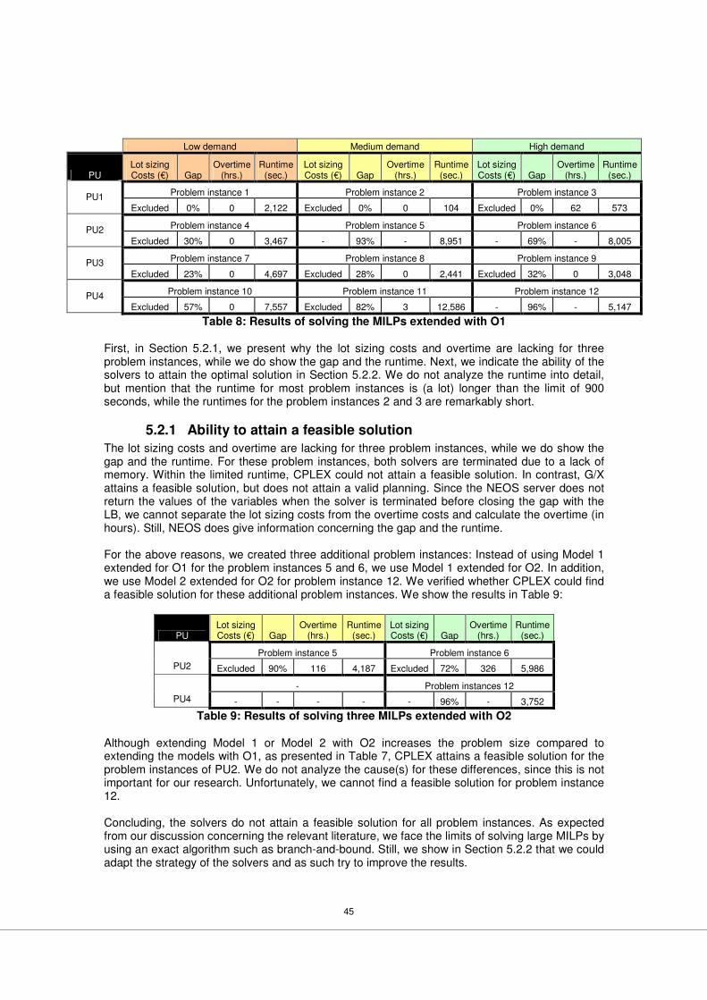
45

Low demand Medium demand High demand

PU Lot sizing Costs (€) Gap

Overtime (hrs.)

Runtime (sec.)

Lot sizing Costs (€) Gap

Overtime (hrs.)

Runtime (sec.)

Lot sizing Costs (€) Gap

Overtime (hrs.)

Runtime (sec.)

Problem instance 1 Problem instance 2 Problem instance 3 PU1 Excluded 0% 0 2,122 Excluded 0% 0 104 Excluded 0% 62 573

Problem instance 4 Problem instance 5 Problem instance 6 PU2 Excluded 30% 0 3,467 - 93% - 8,951 - 69% - 8,005

Problem instance 7 Problem instance 8 Problem instance 9 PU3 Excluded 23% 0 4,697 Excluded 28% 0 2,441 Excluded 32% 0 3,048

Problem instance 10 Problem instance 11 Problem instance 12 PU4 Excluded 57% 0 7,557 Excluded 82% 3 12,586 - 96% - 5,147

Table 8: Results of solving the MILPs extended with O1 First, in Section 5.2.1, we present why the lot sizing costs and overtime are lacking for three problem instances, while we do show the gap and the runtime. Next, we indicate the ability of the solvers to attain the optimal solution in Section 5.2.2. We do not analyze the runtime into detail, but mention that the runtime for most problem instances is (a lot) longer than the limit of 900 seconds, while the runtimes for the problem instances 2 and 3 are remarkably short.

5.2.1 Ability to attain a feasible solution

The lot sizing costs and overtime are lacking for three problem instances, while we do show the gap and the runtime. For these problem instances, both solvers are terminated due to a lack of memory. Within the limited runtime, CPLEX could not attain a feasible solution. In contrast, G/X attains a feasible solution, but does not attain a valid planning. Since the NEOS server does not return the values of the variables when the solver is terminated before closing the gap with the LB, we cannot separate the lot sizing costs from the overtime costs and calculate the overtime (in hours). Still, NEOS does give information concerning the gap and the runtime. For the above reasons, we created three additional problem instances: Instead of using Model 1 extended for O1 for the problem instances 5 and 6, we use Model 1 extended for O2. In addition, we use Model 2 extended for O2 for problem instance 12. We verified whether CPLEX could find a feasible solution for these additional problem instances. We show the results in Table 9:

PU Lot sizing Costs (€) Gap

Overtime (hrs.)

Runtime (sec.)

Lot sizing Costs (€) Gap

Overtime (hrs.)

Runtime (sec.)

Problem instance 5 Problem instance 6 PU2 Excluded 90% 116 4,187 Excluded 72% 326 5,986

- Problem instances 12 PU4 - - - - - 96% - 3,752

Table 9: Results of solving three MILPs extended with O2 Although extending Model 1 or Model 2 with O2 increases the problem size compared to extending the models with O1, as presented in Table 7, CPLEX attains a feasible solution for the problem instances of PU2. We do not analyze the cause(s) for these differences, since this is not important for our research. Unfortunately, we cannot find a feasible solution for problem instance 12. Concluding, the solvers do not attain a feasible solution for all problem instances. As expected from our discussion concerning the relevant literature, we face the limits of solving large MILPs by using an exact algorithm such as branch-and-bound. Still, we show in Section 5.2.2 that we could adapt the strategy of the solvers and as such try to improve the results.

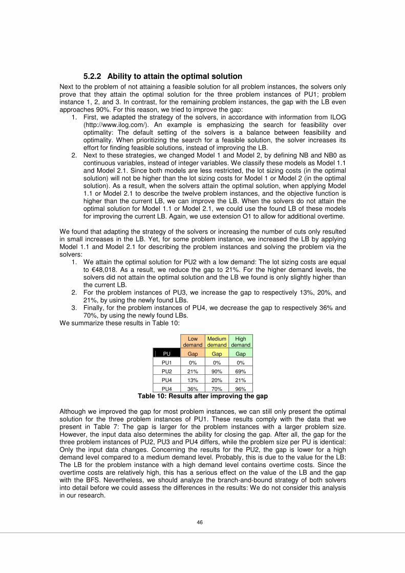
46

5.2.2 Ability to attain the optimal solution

Next to the problem of not attaining a feasible solution for all problem instances, the solvers only prove that they attain the optimal solution for the three problem instances of PU1; problem instance 1, 2, and 3. In contrast, for the remaining problem instances, the gap with the LB even approaches 90%. For this reason, we tried to improve the gap:

1. First, we adapted the strategy of the solvers, in accordance with information from ILOG (http://www.ilog.com/). An example is emphasizing the search for feasibility over optimality: The default setting of the solvers is a balance between feasibility and optimality. When prioritizing the search for a feasible solution, the solver increases its effort for finding feasible solutions, instead of improving the LB.

2. Next to these strategies, we changed Model 1 and Model 2, by defining NB and NB0 as continuous variables, instead of integer variables. We classify these models as Model 1.1 and Model 2.1. Since both models are less restricted, the lot sizing costs (in the optimal solution) will not be higher than the lot sizing costs for Model 1 or Model 2 (in the optimal solution). As a result, when the solvers attain the optimal solution, when applying Model 1.1 or Model 2.1 to describe the twelve problem instances, and the objective function is higher than the current LB, we can improve the LB. When the solvers do not attain the optimal solution for Model 1.1 or Model 2.1, we could use the found LB of these models for improving the current LB. Again, we use extension O1 to allow for additional overtime.

We found that adapting the strategy of the solvers or increasing the number of cuts only resulted in small increases in the LB. Yet, for some problem instance, we increased the LB by applying Model 1.1 and Model 2.1 for describing the problem instances and solving the problem via the solvers:

1. We attain the optimal solution for PU2 with a low demand: The lot sizing costs are equal to €48,018. As a result, we reduce the gap to 21%. For the higher demand levels, the solvers did not attain the optimal solution and the LB we found is only slightly higher than the current LB.

2. For the problem instances of PU3, we increase the gap to respectively 13%, 20%, and 21%, by using the newly found LBs.

3. Finally, for the problem instances of PU4, we decrease the gap to respectively 36% and 70%, by using the newly found LBs.

We summarize these results in Table 10:

Low

demand Medium demand

High demand

PU Gap Gap Gap

PU1 0% 0% 0%

PU2 21% 90% 69%

PU4 13% 20% 21%

PU4 36% 70% 96% Table 10: Results after improving the gap

Although we improved the gap for most problem instances, we can still only present the optimal solution for the three problem instances of PU1. These results comply with the data that we present in Table 7: The gap is larger for the problem instances with a larger problem size. However, the input data also determines the ability for closing the gap. After all, the gap for the three problem instances of PU2, PU3 and PU4 differs, while the problem size per PU is identical: Only the input data changes. Concerning the results for the PU2, the gap is lower for a high demand level compared to a medium demand level. Probably, this is due to the value for the LB: The LB for the problem instance with a high demand level contains overtime costs. Since the overtime costs are relatively high, this has a serious effect on the value of the LB and the gap with the BFS. Nevertheless, we should analyze the branch-and-bound strategy of both solvers into detail before we could assess the differences in the results: We do not consider this analysis in our research.

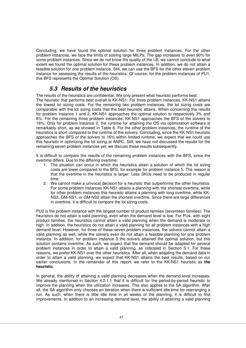
47

Concluding, we have found the optimal solution for three problem instances. For the other problem instances, we face the limits of solving large MILPs: The gap increases to even 90% for some problem instances. Since we do not know the quality of the LB, we cannot conclude to what extent we found the optimal solution for these problem instances. In addition, we do not attain a feasible solution for one problem instance. Still, we can use the BFS for the other eleven problem instance for assessing the results of the heuristics. Of course, for the problem instances of PU1, this BFS represents the Optimal Solution (OS).

5.3 Results of the heuristics The results of the heuristics are confidential: We only present what heuristic performs best: The heuristic that performs best overall is KK-NS1: For three problem instances, KK-NS1 attains the lowest lot sizing costs. For the remaining two problem instances, the lot sizing costs are comparable with the lot sizing costs that the best heuristic attains. When concerning the results for problem instance 1 and 2, KK-NS1 approaches the optimal solution to respectively 3% and 6%. For the remaining three problem instances, KK-NS1 approaches the BFS of the solvers to 16%. Only for problem instance 2, the runtime for attaining the OS via optimization software is remarkably short, as we showed in Table 8. For the other problem instances, the runtime of the heuristics is short compared to the runtime of the solvers. Concluding, since the KK-NS1 heuristic approaches the BFS of the solvers to 16% within limited runtime, we expect that we could use this heuristic in optimizing the lot sizing at ANPC. Still, we have not discussed the results for the remaining seven problem instances yet; we discuss these results subsequently. It is difficult to compare the results of the remaining problem instances with the BFS, since the overtime differs. Due to the differing overtime:

1. The situation can occur in which the heuristics attain a solution of which the lot sizing costs are lower compared to the BFS, for example for problem instance 5. The reason is that the overtime in the heuristics is larger: Less SKUs need to be produced in regular time.

2. We cannot make a univocal decision for a heuristic that outperforms the other heuristics: For some problem instances KK-NS1 attains a planning with the shortest overtime, while for other problem instances this heuristic attains a planning with long overtime, while KK-NS2, GM-NS1, or GM-NS2 attain the shortest overtime. Since there are large differences in overtime, it is difficult to compare the lot sizing costs.

PU2 is the problem instance with the largest number of product families (seventeen families): The heuristics do not attain a valid planning, even when the demand level is low. For PU4, with eight product families, the heuristics cannot attain a valid planning when the demand is moderate or high. In addition, the heuristics do not attain a valid planning for all problem instances with a high demand level. However, for three of these seven problem instances, the solvers cannot attain a valid planning as well, while the solvers even do not attain a feasible planning for one problem instance. In addition, for problem instance 3 the solvers attained the optimal solution, but this solution contains overtime. As such, we expect that the demand should be adapted for several problem instances in order to attain a valid planning, as indicated in Section 5.1. For these reasons, we prefer KK-NS1 over the other heuristics. After all, when adapting the demand data in order to attain a valid planning, we expect that KK-NS1 attains the best results, based on our earlier conclusions. In the remainder of this report, we refer to the KK-NS1 heuristic as the heuristic. In general, the ability of attaining a valid planning decreases when the demand level increases: We already mentioned in Section 4.2.1.1 that it is difficult for the period-by-period heuristic to improve the planning when the utilization increases. This also applies to the SA algorithm. After all, the SA algorithm only chooses an iteration when there is sufficient idle time for rearranging a run. As such, when there is little idle time in all weeks of the planning, it is difficult to find improvements. In addition to an increasing demand level, the ability of attaining a valid planning

48

or finding improvement opportunities decreases when the number of product families increase: When the number of product families increase, the chance that the algorithm considers those iterations that lead to an improvement decreases. Additionally, the SA algorithm is slower when a problem instance contains more product families: We show the number of iterations that the SA algorithm (approximately) considers for the problem instances of every PU in Table 11:

PU #

Iterations

PU1 3,400

PU2 2,000

PU3 3,100

PU4 3,700 Table 11: Number of iterations per PU

Naturally, the choice for the cooling schedule also influences the number of iterations that the SA algorithm considers. Still, for PU2, the number of iterations cannot exceed 2,000 iterations, in order to prevent the runtime to increase above 900 seconds. As such, when the number of product families increases, the number of iterations that the SA algorithm can consider within 900 seconds decreases. Consequently, the ability of the SA algorithm to find improvements decreases as well. Concluding, we prefer the KK-NS1 heuristic over the other heuristics. For the five problem instances for which the heuristics attain a valid planning, KK-NS1 approaches the BFS to respectively 6% and 16%. In addition, the runtime of the heuristics is much shorter compared to the runtime of the solvers. However, the ability of attaining a valid planning decreases when considering more product families. Also, the impact of increasing the demand level is apparent, since the period-by-period heuristic and the SA algorithm cannot find improvements as easily. Yet, we show in Section 5.4 that the comparison with the current performance and the current policy, as defined in Section 2.3, shows promising results. In addition, we present in Section 5.5 that ANPC could still use the results, also when the planning is invalid.

5.4 Assessing the current situation In the previous section, we concluded that we prefer the KK-NS1 heuristic over the other heuristics. In order to verify whether this heuristic could support ANPC in reducing the lot sizing costs, we compare the output of the KK-NS1 heuristic with the current performance and the current policy: We use the actual, unchanged demand data for the last 26 weeks of 2009 to calculate the planning and compare the resulting lot sizing costs with the lot sizing costs of the current performance and the current policy: We define the planning for four problem instances. As discussed before, we do not present our results. However, we indicate how we calculated our results:

1. Regarding the current performance, we use the number of changeovers to calculate the changeover costs. We calculate the inventory costs for storing the inventory excluding the SS, since we excluded the SS form our model.

2. Regarding the current policy, we use the PLT to determine the number of changeovers and use the STs to calculate the inventory costs. We subtract the SS from the STs, in order to determine the accompanying inventory costs.

Thirdly, we calculate the costs of the advised policy, which we define as the policy resulting from calculating the planning with the KK-NS1 heuristic. We discuss two aspects that are notably:

1. The differences between the current performance and the current policy are considerable. However, the current policy is applicable to the last 26 weeks of 2009,

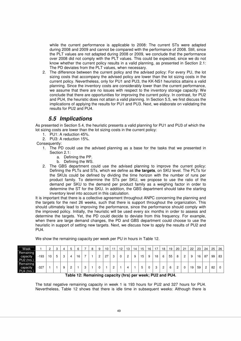
49

while the current performance is applicable to 2008: The current STs were adapted during 2008 and 2009 and cannot be compared with the performance of 2008. Still, since the PLT values are not adapted during 2008 or 2009, we conclude that the performance over 2008 did not comply with the PLT values. This could be expected, since we do not know whether the current policy results in a valid planning, as presented in Section 2.1: The PD deviates from the PLT values, when necessary.

2. The difference between the current policy and the advised policy: For every PU, the lot sizing costs that accompany the advised policy are lower than the lot sizing costs in the current policy. Nevertheless, only for PU1 and PU3, the KK-NS1 heuristics attains a valid planning. Since the inventory costs are considerably lower than the current performance, we assume that there are no issues with respect to the inventory storage capacity: We conclude that there are opportunities for improving the current policy. In contrast, for PU2 and PU4, the heuristic does not attain a valid planning. In Section 5.5, we first discuss the implications of applying the results for PU1 and PU3. Next, we elaborate on validating the results for PU2 and PU4.

5.5 Implications As presented in Section 5.4, the heuristic presents a valid planning for PU1 and PU3 of which the lot sizing costs are lower than the lot sizing costs in the current policy:

1. PU1: A reduction 45%. 2. PU3: A reduction 15%.

Consequently: 1. The PD could use the advised planning as a base for the tasks that we presented in

Section 2.1: a. Defining the PP. b. Defining the WS.

2. The GBS department could use the advised planning to improve the current policy: Defining the PLTs and STs, which we define as the targets, on SKU level. The PLTs for the SKUs could be defined by dividing the time horizon with the number of runs per product family. To determine the STs per SKU, we propose to use the ratio of the demand per SKU to the demand per product family as a weighing factor in order to determine the ST for the SKU. In addition, the GBS department should take the starting inventory level into account in this calculation.

It is important that there is a collective agreement throughout ANPC concerning the planning and the targets for the next 26 weeks, such that there is support throughout the organization. This should ultimately lead to improving the performance, since the performance should comply with the improved policy. Initially, the heuristic will be used every six months in order to assess and determine the targets. Yet, the PD could decide to deviate from this frequency. For example, when there are large demand changes, the PD and GBS department could choose to use the heuristic in support of setting new targets. Next, we discuss how to apply the results of PU2 and PU4. We show the remaining capacity per week per PU in hours in Table 12.

Week 1 2 3 4 5 6 7 8 9 10 11 12 13 14 15 16 17 18 19 20 21 22 23 24 25 26 Remaining capacity

PU2 (hrs.) -193 10 5 3 4 16 7 1 2 27 3 0 2 9 15 9 18 6 55 8 2 9 16 87 99 83

Remaining capacity

PU4 (hrs.) -327 1 1 9 2 1 3 1 0 1 2 1 4 1 5 0 3 2 6 2 0 19 59 2 82 0

Table 12: Remaining capacity (hrs) per week; PU2 and PU4.

The total negative remaining capacity in week 1 is 193 hours for PU2 and 327 hours for PU4. Nevertheless, Table 12 shows that there is idle time in subsequent weeks: Although there is

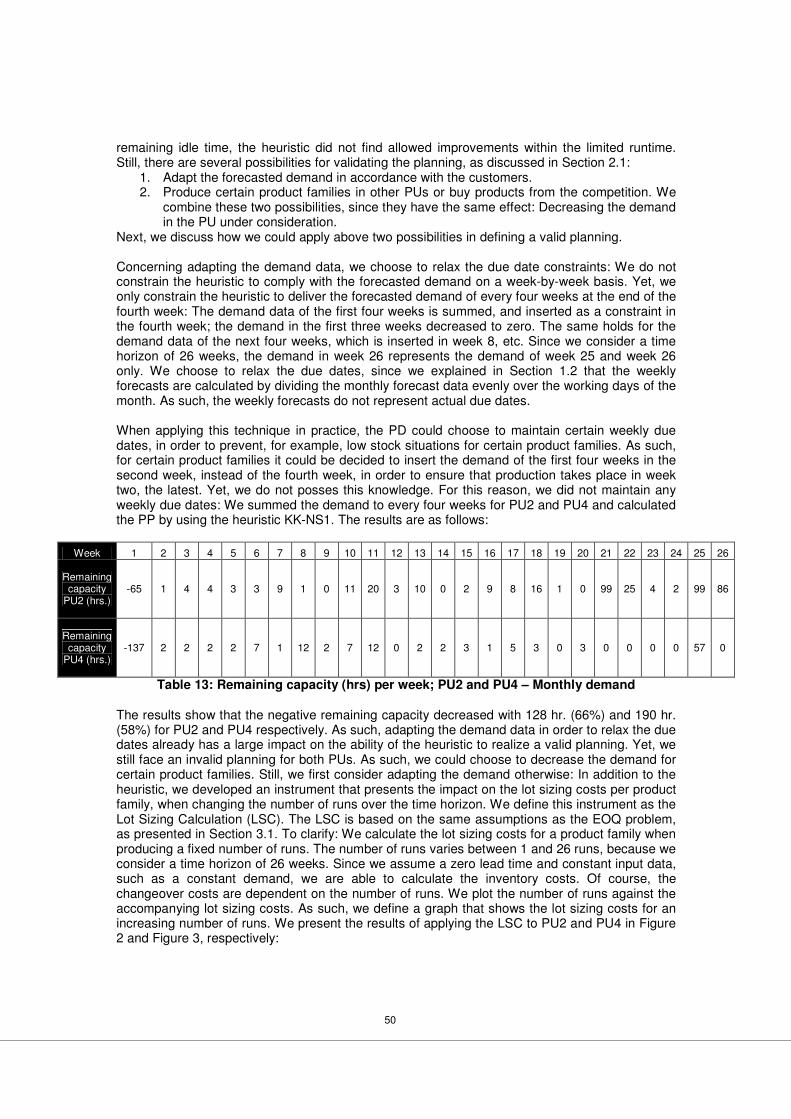
50

remaining idle time, the heuristic did not find allowed improvements within the limited runtime. Still, there are several possibilities for validating the planning, as discussed in Section 2.1:

1. Adapt the forecasted demand in accordance with the customers. 2. Produce certain product families in other PUs or buy products from the competition. We

combine these two possibilities, since they have the same effect: Decreasing the demand in the PU under consideration.

Next, we discuss how we could apply above two possibilities in defining a valid planning. Concerning adapting the demand data, we choose to relax the due date constraints: We do not constrain the heuristic to comply with the forecasted demand on a week-by-week basis. Yet, we only constrain the heuristic to deliver the forecasted demand of every four weeks at the end of the fourth week: The demand data of the first four weeks is summed, and inserted as a constraint in the fourth week; the demand in the first three weeks decreased to zero. The same holds for the demand data of the next four weeks, which is inserted in week 8, etc. Since we consider a time horizon of 26 weeks, the demand in week 26 represents the demand of week 25 and week 26 only. We choose to relax the due dates, since we explained in Section 1.2 that the weekly forecasts are calculated by dividing the monthly forecast data evenly over the working days of the month. As such, the weekly forecasts do not represent actual due dates. When applying this technique in practice, the PD could choose to maintain certain weekly due dates, in order to prevent, for example, low stock situations for certain product families. As such, for certain product families it could be decided to insert the demand of the first four weeks in the second week, instead of the fourth week, in order to ensure that production takes place in week two, the latest. Yet, we do not posses this knowledge. For this reason, we did not maintain any weekly due dates: We summed the demand to every four weeks for PU2 and PU4 and calculated the PP by using the heuristic KK-NS1. The results are as follows:

Week 1 2 3 4 5 6 7 8 9 10 11 12 13 14 15 16 17 18 19 20 21 22 23 24 25 26

Remaining capacity

PU2 (hrs.) -65 1 4 4 3 3 9 1 0 11 20 3 10 0 2 9 8 16 1 0 99 25 4 2 99 86

Remaining capacity

PU4 (hrs.) -137 2 2 2 2 7 1 12 2 7 12 0 2 2 3 1 5 3 0 3 0 0 0 0 57 0

Table 13: Remaining capacity (hrs) per week; PU2 and PU4 – Monthly demand The results show that the negative remaining capacity decreased with 128 hr. (66%) and 190 hr. (58%) for PU2 and PU4 respectively. As such, adapting the demand data in order to relax the due dates already has a large impact on the ability of the heuristic to realize a valid planning. Yet, we still face an invalid planning for both PUs. As such, we could choose to decrease the demand for certain product families. Still, we first consider adapting the demand otherwise: In addition to the heuristic, we developed an instrument that presents the impact on the lot sizing costs per product family, when changing the number of runs over the time horizon. We define this instrument as the Lot Sizing Calculation (LSC). The LSC is based on the same assumptions as the EOQ problem, as presented in Section 3.1. To clarify: We calculate the lot sizing costs for a product family when producing a fixed number of runs. The number of runs varies between 1 and 26 runs, because we consider a time horizon of 26 weeks. Since we assume a zero lead time and constant input data, such as a constant demand, we are able to calculate the inventory costs. Of course, the changeover costs are dependent on the number of runs. We plot the number of runs against the accompanying lot sizing costs. As such, we define a graph that shows the lot sizing costs for an increasing number of runs. We present the results of applying the LSC to PU2 and PU4 in Figure 2 and Figure 3, respectively:

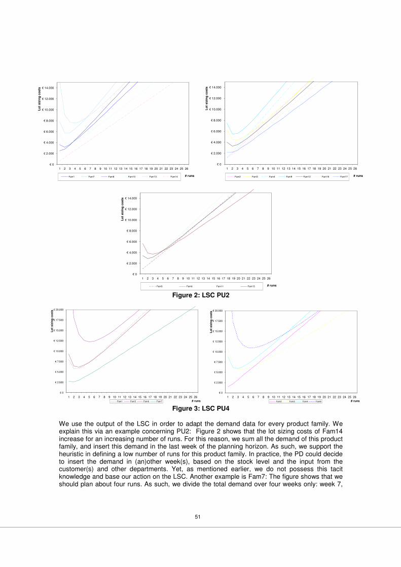
51

€ 0

€ 2.000

€ 4.000

€ 6.000

€ 8.000

€ 10.000

€ 12.000

€ 14.000

1 2 3 4 5 6 7 8 9 10 11 12 13 14 15 16 17 18 19 20 21 22 23 24 25 26

# runs

Lo

t siz

ing

co

sts

Fam1 Fam7 Fam8 Fam10 Fam13 Fam14

€ 0

€ 2.000

€ 4.000

€ 6.000

€ 8.000

€ 10.000

€ 12.000

€ 14.000

1 2 3 4 5 6 7 8 9 10 11 12 13 14 15 16 17 18 19 20 21 22 23 24 25 26

# runs

Lo

t s

izin

g c

osts

Fam2 Fam3 Fam4 Fam9 Fam12 Fam16 Fam17

€ 0

€ 2.000

€ 4.000

€ 6.000

€ 8.000

€ 10.000

€ 12.000

€ 14.000

1 2 3 4 5 6 7 8 9 10 11 12 13 14 15 16 17 18 19 20 21 22 23 24 25 26

# runs

Lo

t siz

ing

co

sts

Fam5 Fam6 Fam11 Fam15

Figure 2: LSC PU2

€ 0

€ 2.500

€ 5.000

€ 7.500

€ 10.000

€ 12.500

€ 15.000

€ 17.500

€ 20.000

1 2 3 4 5 6 7 8 9 10 11 12 13 14 15 16 17 18 19 20 21 22 23 24 25 26# runs

Lo

t siz

ing

co

sts

Fam1 Fam5 Fam6 Fam7

€ 0

€ 2.500

€ 5.000

€ 7.500

€ 10.000

€ 12.500

€ 15.000

€ 17.500

€ 20.000

1 2 3 4 5 6 7 8 9 10 11 12 13 14 15 16 17 18 19 20 21 22 23 24 25 26# runs

Lo

t siz

ing

co

sts

Fam2 Fam3 Fam4 Fam8 Figure 3: LSC PU4

We use the output of the LSC in order to adapt the demand data for every product family. We explain this via an example concerning PU2: Figure 2 shows that the lot sizing costs of Fam14 increase for an increasing number of runs. For this reason, we sum all the demand of this product family, and insert this demand in the last week of the planning horizon. As such, we support the heuristic in defining a low number of runs for this product family. In practice, the PD could decide to insert the demand in (an)other week(s), based on the stock level and the input from the customer(s) and other departments. Yet, as mentioned earlier, we do not possess this tacit knowledge and base our action on the LSC. Another example is Fam7: The figure shows that we should plan about four runs. As such, we divide the total demand over four weeks only: week 7,

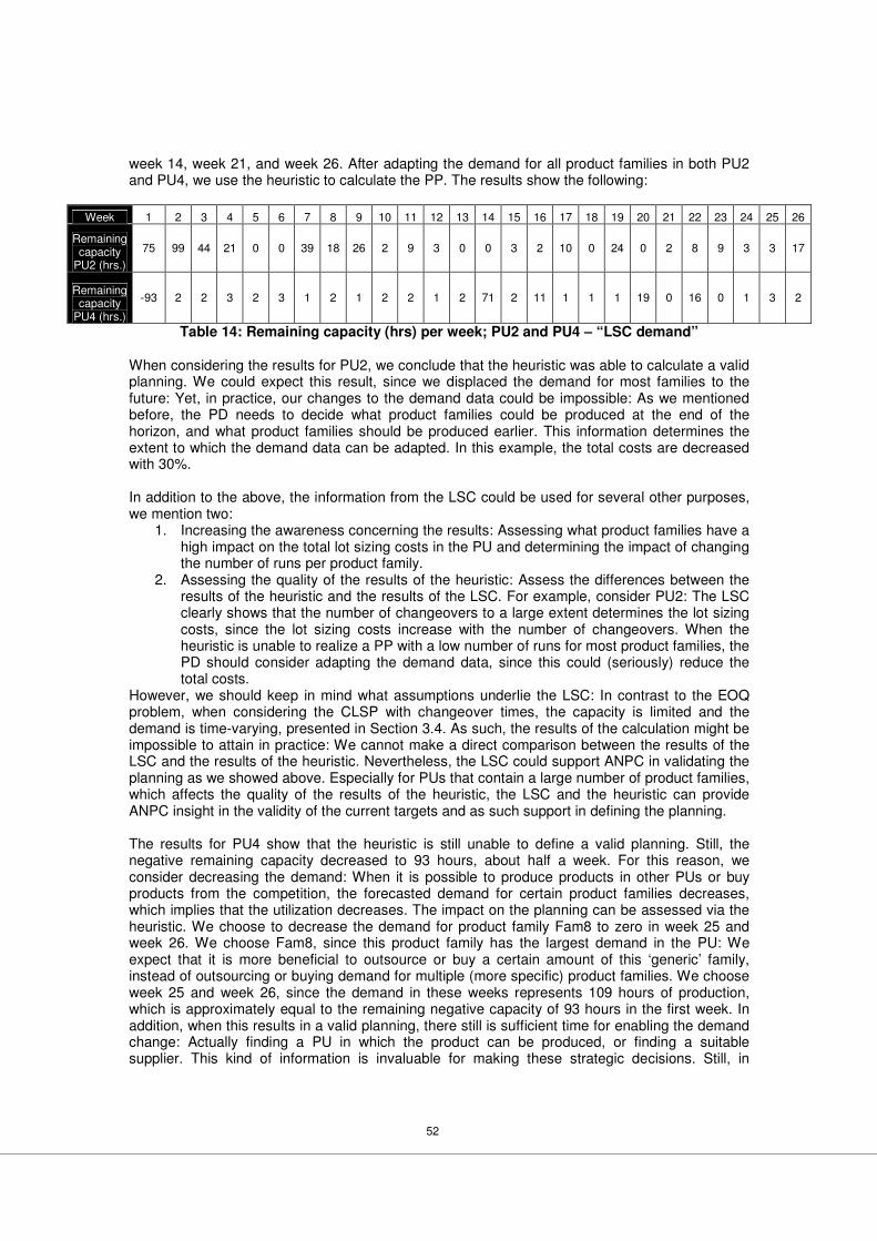
52

week 14, week 21, and week 26. After adapting the demand for all product families in both PU2 and PU4, we use the heuristic to calculate the PP. The results show the following:

Week 1 2 3 4 5 6 7 8 9 10 11 12 13 14 15 16 17 18 19 20 21 22 23 24 25 26

Remaining capacity

PU2 (hrs.)

75 99 44 21 0 0 39 18 26 2 9 3 0 0 3 2 10 0 24 0 2 8 9 3 3 17

Remaining capacity

PU4 (hrs.)

-93 2 2 3 2 3 1 2 1 2 2 1 2 71 2 11 1 1 1 19 0 16 0 1 3 2

Table 14: Remaining capacity (hrs) per week; PU2 and PU4 – “LSC demand” When considering the results for PU2, we conclude that the heuristic was able to calculate a valid planning. We could expect this result, since we displaced the demand for most families to the future: Yet, in practice, our changes to the demand data could be impossible: As we mentioned before, the PD needs to decide what product families could be produced at the end of the horizon, and what product families should be produced earlier. This information determines the extent to which the demand data can be adapted. In this example, the total costs are decreased with 30%. In addition to the above, the information from the LSC could be used for several other purposes, we mention two:

1. Increasing the awareness concerning the results: Assessing what product families have a high impact on the total lot sizing costs in the PU and determining the impact of changing the number of runs per product family.

2. Assessing the quality of the results of the heuristic: Assess the differences between the results of the heuristic and the results of the LSC. For example, consider PU2: The LSC clearly shows that the number of changeovers to a large extent determines the lot sizing costs, since the lot sizing costs increase with the number of changeovers. When the heuristic is unable to realize a PP with a low number of runs for most product families, the PD should consider adapting the demand data, since this could (seriously) reduce the total costs.

However, we should keep in mind what assumptions underlie the LSC: In contrast to the EOQ problem, when considering the CLSP with changeover times, the capacity is limited and the demand is time-varying, presented in Section 3.4. As such, the results of the calculation might be impossible to attain in practice: We cannot make a direct comparison between the results of the LSC and the results of the heuristic. Nevertheless, the LSC could support ANPC in validating the planning as we showed above. Especially for PUs that contain a large number of product families, which affects the quality of the results of the heuristic, the LSC and the heuristic can provide ANPC insight in the validity of the current targets and as such support in defining the planning. The results for PU4 show that the heuristic is still unable to define a valid planning. Still, the negative remaining capacity decreased to 93 hours, about half a week. For this reason, we consider decreasing the demand: When it is possible to produce products in other PUs or buy products from the competition, the forecasted demand for certain product families decreases, which implies that the utilization decreases. The impact on the planning can be assessed via the heuristic. We choose to decrease the demand for product family Fam8 to zero in week 25 and week 26. We choose Fam8, since this product family has the largest demand in the PU: We expect that it is more beneficial to outsource or buy a certain amount of this ‘generic’ family, instead of outsourcing or buying demand for multiple (more specific) product families. We choose week 25 and week 26, since the demand in these weeks represents 109 hours of production, which is approximately equal to the remaining negative capacity of 93 hours in the first week. In addition, when this results in a valid planning, there still is sufficient time for enabling the demand change: Actually finding a PU in which the product can be produced, or finding a suitable supplier. This kind of information is invaluable for making these strategic decisions. Still, in

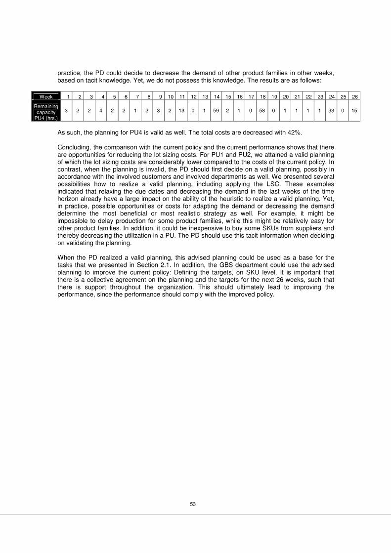
53

practice, the PD could decide to decrease the demand of other product families in other weeks, based on tacit knowledge. Yet, we do not possess this knowledge. The results are as follows:

Week 1 2 3 4 5 6 7 8 9 10 11 12 13 14 15 16 17 18 19 20 21 22 23 24 25 26

Remaining capacity

PU4 (hrs.)

3 2 2 4 2 2 1 2 3 2 13 0 1 59 2 1 0 58 0 1 1 1 1 33 0 15

As such, the planning for PU4 is valid as well. The total costs are decreased with 42%. Concluding, the comparison with the current policy and the current performance shows that there are opportunities for reducing the lot sizing costs. For PU1 and PU2, we attained a valid planning of which the lot sizing costs are considerably lower compared to the costs of the current policy. In contrast, when the planning is invalid, the PD should first decide on a valid planning, possibly in accordance with the involved customers and involved departments as well. We presented several possibilities how to realize a valid planning, including applying the LSC. These examples indicated that relaxing the due dates and decreasing the demand in the last weeks of the time horizon already have a large impact on the ability of the heuristic to realize a valid planning. Yet, in practice, possible opportunities or costs for adapting the demand or decreasing the demand determine the most beneficial or most realistic strategy as well. For example, it might be impossible to delay production for some product families, while this might be relatively easy for other product families. In addition, it could be inexpensive to buy some SKUs from suppliers and thereby decreasing the utilization in a PU. The PD should use this tacit information when deciding on validating the planning. When the PD realized a valid planning, this advised planning could be used as a base for the tasks that we presented in Section 2.1. In addition, the GBS department could use the advised planning to improve the current policy: Defining the targets, on SKU level. It is important that there is a collective agreement on the planning and the targets for the next 26 weeks, such that there is support throughout the organization. This should ultimately lead to improving the performance, since the performance should comply with the improved policy.

54

Chapter 6 Conclusions & Recommendations First, we present the answers to our research questions and indicate to what extent we attain the goal of our research in Section 6.1. In addition, we consider our recommendations in Section 6.2 and possibilities for further research in Section 6.3.

6.1 Conclusions To attain our research goal, we presented four research questions in Section 1.3. In this section, we review our answers for these research questions and indicate to what extent we realize our research goal. In Chapter 2 we describe the current situation regarding the lot sizing: The PD determines a planning (the PP) based on the PLTs and STs for every SKU. The PP defines the runs for the product families and needs to comply with SKU due dates: It functions as a base with which the PD determines the weekly schedule (WS). However, there is insufficient insight in the impact of (changing) the PLT and ST values on the total lot sizing costs. In addition, it is unknown whether defining a planning based on the lot sizing policy leads to a valid planning. After describing the relevant literature in Chapter 3, we conclude that the problem that ANPC faces is the capacitated lot sizing problem with changeover costs and changeover times. This problem is a difficult problem; heuristics seem to be more useful when trying to solve this problem. Next to SA, several relatively simple period-by-period heuristics seem to perform sufficiently well on average, can easily be implemented on a PC, and are fast. For these reasons, we study the possibilities of combining a period-by-period heuristic with a SA algorithm. In order to verify the quality of the different heuristics that we develop, we develop two MILPs as well, and compare the results of solving these MILPs via optimization software with the results of the heuristics. Summarizing, we design two MILPs and six different heuristics in Chapter 4. In Chapter 5, we create twelve problem instances: We chose a low, medium, and high demand level for four PUs. We present the results of solving the MILPs in optimization software and the results of the heuristics:

1. We indicate that we combine the results of two types of solvers: CPLEX and G/X and showed in Section 5.2 that we only attained the optimal solution for three problem instances. For the other PUs, the solvers did not close the gap with the LB: The gap increases to even 90% for some problem instances. In addition, for one problem instance, CPLEX did not attain a feasible solution.

2. For the five problem instances for which the heuristics attain a valid planning, KK-NS1 approaches the optimal solution or best feasible solution to 16%. In addition, for two of these problem instances, this heuristic approaches the optimal solution to respectively 3% and 6%. Moreover, the runtime of the heuristic is much shorter compared to the runtime of the solvers. For the seven remaining problem instances, no heuristic attains a valid planning. In general, the ability of the heuristics for attaining a valid planning decreases when considering more product families. Also, the impact of increasing the demand level is apparent, since the period-by-period heuristic and the SA algorithm cannot find feasible improvements as easily when the demand increases. Still, one heuristic showed to outperform the other heuristics for the problem instances for which the heuristics attained a valid planning: The KK-NS1 heuristic.

When comparing the output of the KK-NS1 heuristic with the current performance and the current policy, we conclude that there are opportunities for improving the current policy and as such reducing the lot sizing costs: For every PU, the lot sizing costs that accompany the advised planning, as defined in Section 2.1, are lower compared to the lot sizing costs in the current policy. The results for PU1 and PU3 show that the current policy could be improved with respectively 45% and 15%. In contrast to these results, the heuristic did not attain a valid

55

planning for PU2 and PU4. Yet, we present several possibilities for realizing a valid planning, including applying the LSC. As such, we presented a valid planning for both PUs that indicates that the current policy for PU2 and PU4 could be improved by 30% and 45% respectively. Still, in practice, the opportunities or costs for adapting the demand or decreasing the demand influence this decision as well. Concluding, the heuristic and the LSC analysis contribute to solving the issues that we found at ANPC by giving insight in the relation between the choice for the lot sizes and the accompanying costs. As such, we support ANPC in improving the quantity and timing of production orders. The results show that our solution could be used in decreasing the total lot sizing costs at ANPC. In addition, the results support the two remaining PUs that we study in defining a valid planning and reducing the lot sizing costs. As such, we recommend that the heuristic is implemented in the other PUs of ANPC as well. Given that there are 31 other PUs around the globe in which the heuristic can be applied, we anticipate that the contribution that the heuristic can deliver is promising.

6.2 Recommendations Our research shows that there are opportunities for improving the current policy and reducing the lot sizing costs. When the planning is valid, the PD could use the output for defining the planning and the weekly schedule, while the GBS department uses the results for defining the targets. When the planning is invalid, the PD should decide how to adapt the demand data, in accordance with the involved customers. We recommend that the PD of ANPC:

1. Increases the insight in the lot sizing costs by quantifying the inventory and changeover costs.

2. Applies the heuristic and as such obtains a realistic overview of the lot sizing costs and the capacity impact that can be expected in the coming 26 weeks. In addition, since it is straightforward to adapt the data, such as the demand data, the heuristic could be used to assess the consequences of changes in demand or, for example, a possible decrease in availability. Furthermore, especially for PUs that contain a large number of product families, the LSC can provide ANPC with insight in the validity of the current targets. Consequently, the LSC supports ANPC in defining the planning when the quality of the results of the heuristic decreases.

3. Uses the advised planning and the insight in the costs of the results, in order to decide on the PP and the WS, instead of defining the PP and the WS based on the PLTs and STs of which the relation with the total lot sizing costs is unknown. The GBS department can calculate the average inventory levels and PLTs from the advised planning, in order to determine the targets. As a consequence, we support the PD in managing the lot sizing costs, and increase the validity of the lot sizing policy.

We developed an instruction manual that supports ANPC in applying the heuristic in practice. This manual describes the problem, the input data, how to collect the input data, a guideline concerning the execution of the heuristic, the results that are displayed, and how the results could be used. As mentioned, we do not know to what extent the heuristic attains the optimal solution, due to the problem size of the problems that we face. However, the results of our research do provide a first step towards improving the lot sizes, since the results of the heuristic indicate improvement opportunities regarding reducing the changeover and inventory costs. When ANPC applies the improvement opportunities in practice, they could decide to look for further improvement opportunities. We present these possibilities for further research in Section 6.3.

6.3 Future research In our research, we considered improving the lot sizing at ANPC. We developed two MILPs and developed several heuristics in order to analyze how we could best improve the lot sizing. Nevertheless, we did not research all areas that are related to the lot sizing decision. For this reason, we consider the recommendations for future research in this section.

56

1. Optimizing the lot sizing: We recommend that ANPC focuses on improving the lot sizing via improving the information sharing concerning the orders and increasing insight in the lot sizing costs throughout the complete supply chain. For example, when customers adapt their order pattern to comply with the batch sizes, this could directly reduce the inventory levels. In addition, ANPC could collaborate with its customers in defining an order pattern that reduces changeover and inventory costs: Making ANPC responsible for the inventory at the customer. Of course, this is not a transition that is made overnight, but there could be possibilities for improving the lot sizing. On the other hand, since the changeovers affect the availability of the unit and imply direct costs as well, ANPC should continuously search for reducing the changeover times. Actually, when the production process would become more flexible, the problem size could be decreased, since the necessity for modeling the changeovers disappears. 2. Safety Stock: As explained in Section 2.2, we did not include the SS in our research: Currently, the formula with which the SS could be determined is not used, since the formula does not cover all variation, for example the variation in the production process. In addition, there might be more flexibility in defining the planning than the fixed PLT suggests, since the PD is allowed to deviate from the PLT values. Moreover, the SS might be part of a contractual agreement with the customers. As such, when the targets or the planning changes, this does not imply that the SS changes. Still, we recommend that the GBS department, in accordance with the PD and the Sales department, researches how to quantify the determination of the SS, in order to create univocal rules. It could be decided that the determination of the SS levels and the lot sizing decision are interdependent. For example, decreasing the PLTs for some SKUs could imply a decrease in the accompanying SSs, since the SS needs to cover the variation over a shorter PLT. As such, ANPC should define a solution that combines both the determination of the SS levels, as well as the lot sizing decision. 3. Inventory costs: We showed in Section 2.3 that the approach that ANPC takes in defining the inventory costs does not completely comply with the information from the relevant literature. For this reason, ANPC could research whether pricing the inventory value for the capital costs only is a correct representation of reality. In addition, they could analyze whether to define the inventory value based on solely the variable inventory costs, or still include the fixed costs as well. 4. Raw materials: We indicated in Section 2.2 that we assumed that the availability of the raw materials is not an issue when deciding on the planning. Still, storing raw materials also implies inventory costs, while placing orders could imply ordering costs. In fact, the problem of determining the quantity and timing of the orders for the raw materials is comparable with the problem of determining the lot sizes for the product families. For this reason, ANPC could use the heuristic that we developed in this research for gaining insight in the relation between the inventory costs and the ordering costs concerning the raw materials. Ultimately, ANPC could analyze the possibilities for developing solutions for a multi-level problem that includes multiple echelons of the supply chain. Yet, this increases the problem size. 5. Simulated Annealing: In our research, we analyzed the impact of using different starting solutions and different NS-methods in SA. However, there are still lots of other possibilities for defining the starting solution or the choice for the NSs. For example, one option is to allow NSs that could lead to (additional) overtime in every week of the horizon, instead of only allowing for NSs that do not deteriorate the validity of the planning. Another option is choosing those NSs that increase the idle time in the first weeks of the model horizon. Regarding the choice for the starting solution, ANPC could research whether it is possible to develop a starting solution in which the overtime in the first week is minimized. Next to being unable of testing all different options for starting solution or choosing NSs, we did not test all possible cooling schedules for the SA algorithm. Although the tests we performed already give a good indication of the impact that different combinations of the cooling schedules have on the results, the tests are not exhaustive.

57

References Bahl, H.C., Ritzman, and L.P., Gupta, J.N.D. (1986). Determining Lot Sizes and Resource Requirements: A Review. Operations Research 35(3), 329-345.

Bitran, G.B. and Yanasse, H.H. (1982). Computational Complexity of the Capacitated Lot Size Problem. Management Science 28(10), 1174-1186.

Cerny, V. (1985). Thermodynamical Appraoch to the Travelling Salesman Problem: An Efficient Simulation Algorithm. Journal of Optimization Theory and Applications 45(1), 41-51.

Chen, P., Papageorgiou, and L.G., Pinto, J.M. (2008). Medium-term Planning of Single-stage Single-unit Multiproduct Plants using a Hybrid Discrete/Continuous MILP Model. Ind. and Eng. Chemistry Research 47, 1925-1934.

Coyle, J.J., Bardi, E.J., and Langley Jr, C.J. (2003). The management of business logistics. 7th edition. Toronto: Thomson Learning.

Czyzyk, J., Mesner, M.P., and Moré, J.J. (1998). The NEOS Server. IEEE computational science and engineering July-September, 68-75

Diaby, M., Bahl, H.C., Karwan, M.H., and Zionts, S. (1992). A Lagrangean Approach for Very-large-scale Capacitated Lot-sizing. Management Science 38(9), 1329-1340.

Dixon, P.S. and Silver, E.A. (1981). A Heuristic Solution Procedure for the Multi-item, Single-level, Limited-capacity, Lot-sizing Problem. Journal of Operations Management 2, 23-39.

Drexl, A., and Kimms, A. (1997). Lot Sizing and Scheduling – Survey and Extensions. European Journal of Operational Research 99, 221-235.

Dogramaci, A., Panayiotopoulos, J.C., and Adam, N.R. (1981). The Dynamic Lotsizing Problem for Multiple Items under Limited Capacity. AIIE Transactions 13, 294-303.

Eisenhut, P.S. (1975). A Dynamic Lot Sizing Algorithm with Capacity Constraints. AIIE Transactions 7, 170-176.

Florian, M,. Lenstra, J.K., and Rinnooy Kan, A.H.G. (1980). Deterministic Production Planning: Algorithms and Complexity. Management Science 26(7), 669-679.

Garey, M. and Johnson, D. (1979). Computers and Intractability: A Guide to the Theory of NP-Completeness. Freeman and Co., San Fransisco, CA.

Glover, F. (1990). Tabu Search: A Tutorial. Interfaces 20, 74-94.

Gopalakrishnan, M., Miller, D.M., and Schmidt, C.P. (1995). A Framework for Modeling Setup Carryover in the Capacitated Lot Sizing Problem. International Journal of Production Research 33(7), 1973-1988.

Gopalakrishnan, M., Ding, K., Bourjolly, J., and Mohan, S. (2001). A Tabu-Search Heuristic for the Capacitated Lot-Sizing Problem with Set-up Carryover. Management Science 47(6), 851-863.

Graves, S.C. (1981). A Review of Production Scheduling. Operations Research 29(4), 646-675.

Gupta, D., and Magnusson, T. (2005). The Capacitated Lot-sizing and Scheduling Problem with Sequence-dependent Setup Costs and Setup Times. Computers and Operations Research 32, 727-747.

Harris, F.W. (1913). What quantity to make at once. Factory, the magazine of management Series 10(2), 135-6.

Hopp, W.J. and Spearman, M.L. (2001). Factory Physics. 2nd edition. New York: Irwin/McGraw-Hill.

58

Jans, R., and Degraeve, Z. (2005). Modeling Industrial Lot Sizing Problems: A Review. Erasmus Research Institue of Management (ERIM).

Karimi, B., Fatemi Ghomi, S.M.T., and Wilson, J.M. (2003). The Capacitated Lot Sizing Problem: A Review of Models and Algorithms. Omega 31, 365-378.

Kim, D.-W., Kim, K.-H., Jang, W., and Chen, F.F. (2002). Unrelated parallel machine scheduling with setup times using simulated annealing. Robotics and Computer Integrated Manufacturing 18, 223-231. Kirca, Ö. (1990). An Efficient Algorithm for the Capacitated Single Item Dynamic Lot Size Problem. European Journal of Operational Research 45(1), 15-34. Research 45/1 (1990) 15-34.

Kirca, Ö. and Kökten, M. (1992). A New Heuristic Approach for the Multi-item Dynamic Lot Sizing Problem. European Journal of Operations Research 75, 332-341.

Kirkpatrick, S., Gelatt, C.D., and Vecchi, M.P. (1983). Optimization by Simulated Annealing. Science 220(4598), 671-680.

Kuik, R., and Salomon, S. (1990). Multi-level Lot-sizing Problem: Evaluation of a Simulated-annealing Heuristic. European Journal of Operational Research 45, 25-37.

Kuik, R., and Salomon, S. (1994). Batching Decision: Structure and Models. European Journal of Operational Research 75, 243-263.

Van Laarhoven, P.J.M., and Aarts, E.H.L. (1987). Simulated Annealing: Theory and Applications. Dordrecht, The Netherlands: Kluwer Academic Publishers.

Lambrecht, M.R., and VanderVeken, H. (1979). Heuristic Procedures for the Single Operation Multi-item Loading Problem. AIIE Transactions 11, 319-326.

Liu, S., Pinto, J.M., and Papageorgiou, G. (2008). A TSP-based MILP Model for Medium-term Planning of Single-stage Continuous Multiproduct Plants. Industrial and Engineering Chemistry Research 47, 7733-7743.

Maes, J. and Van Wassenhove, L. (1986). A Simple Heuristic for the Multi-item Single Level Capacitated Lot Sizing Problem. Operations Research Letters 4(6), 265-273.

Maes, J. and Van Wassenhove, L. (1988). Multi-item Single-level Capacitated Dynamic Lot-sizing Heuristics: A General Review. OR Society 39(11) 991-1004

Metropolis, N., Rosenbluth, A., Rosenbluth, M., Teller, A., and Teller, E. (1953). Equation of State Calculations by Fast Computing Machines. The Journal of Chemical Physics 21(6), 1087-1092.

Meyr, H. (2000). Simultaneous Lotsizing and Scheduling by Combining Local Search with Dual Reoptimization. European Journal of Operational Research 120, 311-326.

Özdamar, L. and Bozyel, M.A. (1999). The Capacitated Lot Sizing Problem with Overtime Decisions and Setup Times. IEEE transactions 32, 1043-1057.

Pinedo, M.L. (2005). Springer Series in Operations Research. Planning and scheduling in manufacturing and services. New York: Springer.

Schuur, P.C. (2007). Combinatorische Optimalisering. Reader DOBP. Universiteit Twente, faculteit der technische bedrijfskunde.

Salomon, S., Kuik, R., and Van Wassenhove, L. (1993). Statistical Search Methods for Lotsizing problems. Annales of Operations Research. 41(1), 453-468.

Silver, E.A., Pyke, and D.F., Peterson, R. (1998). Inventory management and production planning and scheduling. Wiley, New York.

Silver, E.A. and Meal, H. (1973). A Heuristic for Selecting Lot-size Quantities for the Case of a Deterministic Time-varying Demand Rate and Discrete Opportunities for Replenishment. Production and inventory management 12(2) 64-74.

59

Tan, K.C., and Narasimhan, R. (1997). Minimizing Tardiness on a Single Processor with Sequence-dependent Setup Times: a Simulated Annealing Approach. Management Science 25(6), 619-634.

Tang, O. (2004). Simulated Annealing in Lot Sizing Problems. Internationl Journal of Production Economics 88, 173-181.

Thizy, J.M. and Van Wassenhove, L.N. (1985). Lagrangean Relaxation for the Multi-item Capacitated Lotsizing Problem: A Heuristic Approach. AIIE Transactions 17, 308-313.

Tijms, H.C. (2004). Inleiding in de operational analyse. Reader DOBP. Universiteit Twente, faculteit der technische bedrijfskunde.

Trigeiro, W.W., Thomas, L.J., and McClain, J.O. (1989). Lot Sizing with Setup Times. Management Science 35(3), 353-366.

Wagner, H.M. and Whitin, T.M. (1958). Dynamic Version of the Economic Lot Size Model. Management Science 5(1) 89-96.

Winston, W.L. (2004). Operations Research. Applications and Algorithms. 4th edition. Toronto: Thomson learning.

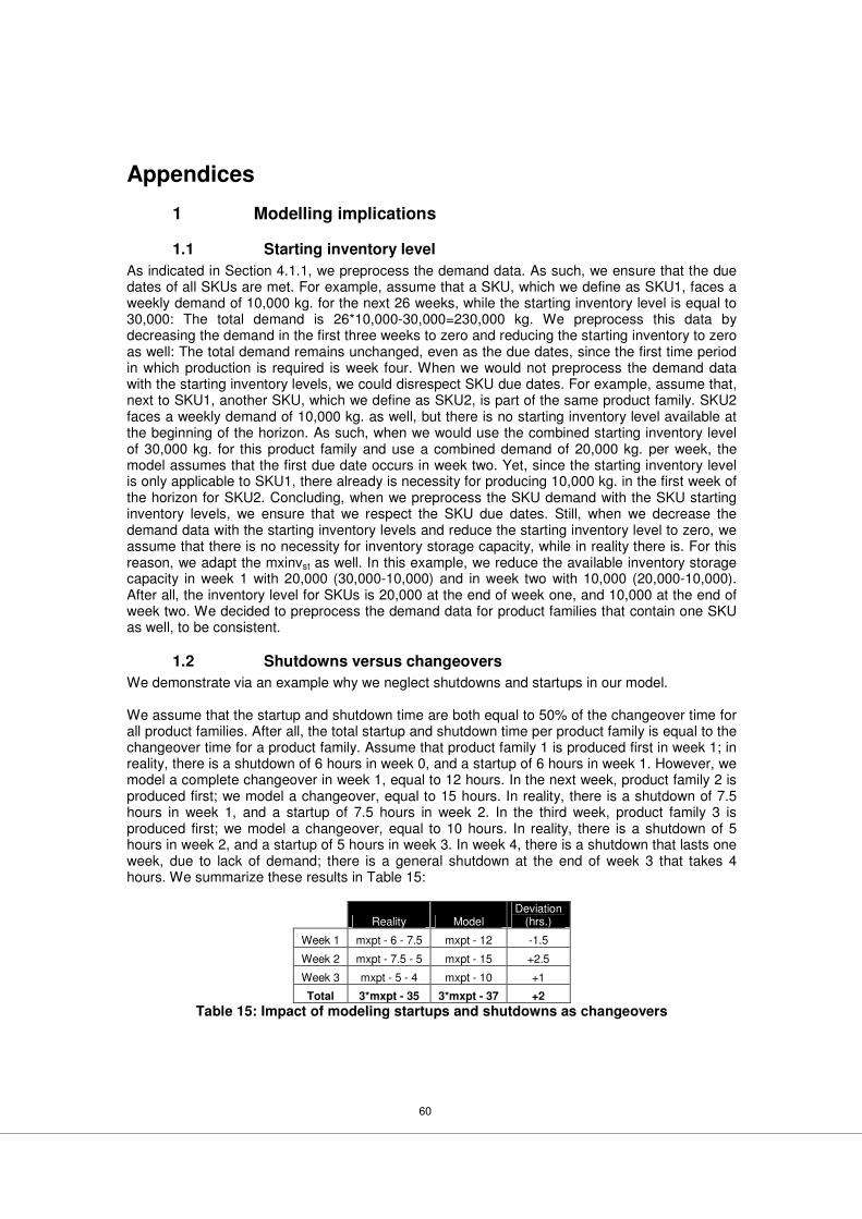
60

Appendices

1 Modelling implications

1.1 Starting inventory level

As indicated in Section 4.1.1, we preprocess the demand data. As such, we ensure that the due dates of all SKUs are met. For example, assume that a SKU, which we define as SKU1, faces a weekly demand of 10,000 kg. for the next 26 weeks, while the starting inventory level is equal to 30,000: The total demand is 26*10,000-30,000=230,000 kg. We preprocess this data by decreasing the demand in the first three weeks to zero and reducing the starting inventory to zero as well: The total demand remains unchanged, even as the due dates, since the first time period in which production is required is week four. When we would not preprocess the demand data with the starting inventory levels, we could disrespect SKU due dates. For example, assume that, next to SKU1, another SKU, which we define as SKU2, is part of the same product family. SKU2 faces a weekly demand of 10,000 kg. as well, but there is no starting inventory level available at the beginning of the horizon. As such, when we would use the combined starting inventory level of 30,000 kg. for this product family and use a combined demand of 20,000 kg. per week, the model assumes that the first due date occurs in week two. Yet, since the starting inventory level is only applicable to SKU1, there already is necessity for producing 10,000 kg. in the first week of the horizon for SKU2. Concluding, when we preprocess the SKU demand with the SKU starting inventory levels, we ensure that we respect the SKU due dates. Still, when we decrease the demand data with the starting inventory levels and reduce the starting inventory level to zero, we assume that there is no necessity for inventory storage capacity, while in reality there is. For this reason, we adapt the mxinvst as well. In this example, we reduce the available inventory storage capacity in week 1 with 20,000 (30,000-10,000) and in week two with 10,000 (20,000-10,000). After all, the inventory level for SKUs is 20,000 at the end of week one, and 10,000 at the end of week two. We decided to preprocess the demand data for product families that contain one SKU as well, to be consistent.

1.2 Shutdowns versus changeovers

We demonstrate via an example why we neglect shutdowns and startups in our model. We assume that the startup and shutdown time are both equal to 50% of the changeover time for all product families. After all, the total startup and shutdown time per product family is equal to the changeover time for a product family. Assume that product family 1 is produced first in week 1; in reality, there is a shutdown of 6 hours in week 0, and a startup of 6 hours in week 1. However, we model a complete changeover in week 1, equal to 12 hours. In the next week, product family 2 is produced first; we model a changeover, equal to 15 hours. In reality, there is a shutdown of 7.5 hours in week 1, and a startup of 7.5 hours in week 2. In the third week, product family 3 is produced first; we model a changeover, equal to 10 hours. In reality, there is a shutdown of 5 hours in week 2, and a startup of 5 hours in week 3. In week 4, there is a shutdown that lasts one week, due to lack of demand; there is a general shutdown at the end of week 3 that takes 4 hours. We summarize these results in Table 15:

Reality Model Deviation

(hrs.)

Week 1 mxpt - 6 - 7.5 mxpt - 12 -1.5

Week 2 mxpt - 7.5 - 5 mxpt - 15 +2.5

Week 3 mxpt - 5 - 4 mxpt - 10 +1

Total 3*mxpt - 35 3*mxpt - 37 +2

Table 15: Impact of modeling startups and shutdowns as changeovers

61

We conclude that the total difference between the startup and shutdown time in reality and the changeover time in the model is equal to the difference between the shutdown time in week 0 and the shutdown time in the last week of the horizon; in this example 6-4 hours = 2 hours. As a result, the deviation over the complete horizon is small. Yet, as we show in our example, there can be deviations from one week to another. However, since changeover times are in the order of 5 to 15 hours, these deviations are small as well; approximately 0% to 5% of the mxpt. In addition, these deviations may cancel out from one week to another, when the changeover time for the product family that is produced first in the week increases and decreases every next week, as we show in our example. As mentioned, we accept these deviations, such that we limit the problem size.

62

2 Penalty costs for production in overtime

It is not straightforward to quantify the penalty costs. Naturally, when we would define the penalty costs to be equal to the changeover costs, producing one batch in overtime is equally priced as producing one batch in regular time. We want to exclude this possibility from the model; the penalty costs for producing one batch of a product family should be higher then the changeover costs for a product family. As a result, we could argue that producing one batch in overtime results in penalty costs that are equal to two changeovers. As a result, producing one batch in overtime in a week results into twice the changeover costs, compared to producing one batch in regular time in the same week. When we consider more batches, the difference increases. For example, producing two batches in overtime results in an increase in (penalty) costs that is equal to four changeovers. Yet, we still cannot be sure that a product family is only produced in overtime, when absolutely necessary. After all, the changeover costs for product families deviate. As a result, when we produce a product family with low changeover costs in overtime, and thereby can prevent the necessity for an expensive changeover in another week, the total costs could be lower, compared to producing all product families in regular time. In addition, we face the inventory costs. That is, when the model has to schedule a number of batches in overtime, it will schedule the production, such that the resulting inventory costs are minimized. However, when there is a possibility for producing these batches, for example, one month earlier in regular time, the model should choose this option, as mentioned in Section 4.1.3. To conclude, we need to ensure that the penalty costs are higher than the possible savings in changeover and inventory costs when producing in overtime. For this reason, we choose the penalty costs to be equal to ten times the maximum changeover costs, plus ten times the maximum inventory holding costs, for storing one batch over the complete model horizon.

63

3 Optimization software

In this appendix, we discuss the optimization software that we use for solving the different problem instances that we consider in our research. First, we discuss the NEOS server and the G/X solver. Next, we discuss the CPLEX solver. Third, we give some general information concerning the output of both solvers.

3.1 NEOS and G/X

According to Czyzyk et al. (1998) the Network-Enabled Optimization System (NEOS) provides users access to optimization software via the NEOS server. The NEOS server resides at Argonne National Laboratory, Northwestern University, and the University of Wisconsin. All solvers can be found at http://neos.mcs.anl.gov/neos/solvers/index.html. Users can submit problems in various formats to the NEOS server; via e-mail or an internet browser. The server checks the input, executes the solver, and returns the solution to the user. The solver we use for our MILP models is the G/X linear and mixed-integer programming solver that is based on the XPRESS-MP Optimization Subroutine Library developed by Dash Associates (http://www.gams.com/dd/docs/solvers/xpress.pdf). The G/X solver runs in conjunction with the General Algebraic Modeling System (GAMS) modeling system, a high level-modeling system for mathematical programming and optimization (http://www.gams.com).

3.2 CPLEX 10

Initially, CPLEX was developed by Robert E. Brixby, and acquired by ILOG in 1997. From January 2009, CPLEX was acquired by IBM. GAMS provides a solver manual concerning CPLEX via their website. The manual indicates that CPLEX is capable of processing different problems, such as LP and MILP. Concerning MILP, CPLEX uses a branch and cut algorithm. More information can be found via http://www.ilog.com/products/cplex/.

3.3 Branch-and-bound

Both solvers are based on the branch-and-bound process. According to Tijms (2004), the basic idea of this method is dividing the total set of feasible solutions in subsets, and eliminating subsets during this process; creating a branch-and-bound tree. Subsets are eliminated via the use of bounds. For more information, we refer to his work. Both solvers use the solution for the LP-relaxation as the root of the tree: The LP-relaxation is the solution to the problem in which the integer variables are replaced for continuous variables; the binary variable are allowed to be continuous on the interval [0,1]. Still, both solvers offer diverse options to, for example, adapt the strategy of defining the root solution, or defining the choice for the subsets that are considered first.