Embed Size (px)
Citation preview

Motivation Lot Sizing Games
Lot Sizing Games
Margarida Carvalho 1 Mathieu Van Vyve 2
Claudio Telha 2
1Faculdade de Ciencias da Universidade do Porto and INESC TEC 2CORE, Universite catholique de Louvain
5th Porto Meeting on MATHEMATICS for INDUSTRYApril, 2014
Margarida Carvalho [email protected] Lot Sizing Games

Motivation Lot Sizing Games
1 MotivationGame Theory and Operational ResearchInteger Programming GamesState of the art
2 Lot Sizing GamesFormulationSolution Concept: Nash equilibriaOne Period GameT Period GameFuture work
Margarida Carvalho [email protected] Lot Sizing Games

Motivation Lot Sizing Games
Game Theory
Game Theory Generalization of decision theory; an individual’ssuccess depends on the choices of others.
1838 Cournot Duopoly (simultaneous game): earliestexamples of game analysis;
1952 Stackelberg Game (sequential game): a player, calledthe leader, takes his decision before decisions of otherplayers, called the followers, are known;
Margarida Carvalho [email protected] Lot Sizing Games

Motivation Lot Sizing Games
Motivation: Integer Programming Games
Normal form games: explicit specification of the players’ pure strategies.
Player IICooperates Defects
Player I
Cooperates 1 1 3 0
Defects 0 3 2 2
Integer Programming Games: players’ pure strategies are lattice points insidepolytopes described by systems of linear inequalities.
Margarida Carvalho [email protected] Lot Sizing Games

Motivation Lot Sizing Games
Integer Programming games
Each player p solves a problem in the form of
Maximizexp Πp(xp, x−p
)
subject to Apxp ≤ bp
xpi integer , ∀i
Margarida Carvalho [email protected] Lot Sizing Games

Motivation Lot Sizing Games
State of Art
There are general methods to solve finite games:
1964 Lemke and Howson;
1991 Elzen and Talman;
2003 Global Newton method by Govindan and Wilson ;
However an explicit description of the set of strategies is required.
Margarida Carvalho [email protected] Lot Sizing Games

Lot Sizing Game: Model
1
2 t T
yp1
F p1
xp1
+cp1
qp1P (Q1)
hp1
Hp1
yp2
F p2
xp2
+cp2
qp2P (Q2)
hp2 hp
t−1
ypt xpt
F pt +cpt
qptP (Qt)
hpt hp
T−1
Hp2 Hp
t−1 Hpt Hp
T−1
ypT
F pT
xpT
+cpT
qpTP (QT )

Lot Sizing Game: Model
1 2
t T
yp1
F p1
xp1
+cp1
qp1P (Q1)
hp1
Hp1
yp2
F p2
xp2
+cp2
qp2P (Q2)
hp2 hp
t−1
ypt xpt
F pt +cpt
qptP (Qt)
hpt hp
T−1
Hp2 Hp
t−1 Hpt Hp
T−1
ypT
F pT
xpT
+cpT
qpTP (QT )

Lot Sizing Game: Model
1 2 t
T
yp1
F p1
xp1
+cp1
qp1P (Q1)
hp1
Hp1
yp2
F p2
xp2
+cp2
qp2P (Q2)
hp2 hp
t−1
ypt xpt
F pt +cpt
qptP (Qt)
hpt hp
T−1
Hp2 Hp
t−1 Hpt Hp
T−1
ypT
F pT
xpT
+cpT
qpTP (QT )

Lot Sizing Game: Model
1 2 t T
yp1
F p1
xp1
+cp1
qp1P (Q1)
hp1
Hp1
yp2
F p2
xp2
+cp2
qp2P (Q2)
hp2 hp
t−1
ypt xpt
F pt +cpt
qptP (Qt)
hpt hp
T−1
Hp2 Hp
t−1 Hpt Hp
T−1
ypT
F pT
xpT
+cpT
qpTP (QT )

Lot Sizing Game: Model
1 2 t T
yp1
F p1
xp1
+cp1
qp1P (Q1)
hp1
Hp1
yp2
F p2
xp2
+cp2
qp2P (Q2)
hp2 hp
t−1
ypt xpt
F pt +cpt
qptP (Qt)
hpt hp
T−1
Hp2 Hp
t−1 Hpt Hp
T−1
ypT
F pT
xpT
+cpT
qpTP (QT )

Lot Sizing Game: Model
1 2 t T
yp1
F p1
xp1
+cp1
qp1P (Q1)
hp1
Hp1
yp2
F p2
xp2
+cp2
qp2P (Q2)
hp2 hp
t−1
ypt xpt
F pt +cpt
qptP (Qt)
hpt hp
T−1
Hp2 Hp
t−1 Hpt Hp
T−1
ypT
F pT
xpT
+cpT
qpTP (QT )

Lot Sizing Game: Model
1 2 t T
yp1
F p1
xp1
+cp1
qp1P (Q1)
hp1
Hp1
yp2
F p2
xp2
+cp2
qp2P (Q2)
hp2 hp
t−1
ypt xpt
F pt +cpt
qptP (Qt)
hpt hp
T−1
Hp2 Hp
t−1 Hpt Hp
T−1
ypT
F pT
xpT
+cpT
qpTP (QT )

Lot Sizing Game: Model
1 2 t T
yp1
F p1
xp1
+cp1
qp1P (Q1)
hp1
Hp1
yp2
F p2
xp2
+cp2
qp2P (Q2)
hp2 hp
t−1
ypt xpt
F pt +cpt
qptP (Qt)
hpt hp
T−1
Hp2 Hp
t−1 Hpt Hp
T−1
ypT
F pT
xpT
+cpT
qpTP (QT )

Lot Sizing Game: Model
1 2 t T
yp1
F p1
xp1
+cp1
qp1P (Q1)
hp1
Hp1
yp2
F p2
xp2
+cp2
qp2P (Q2)
hp2 hp
t−1
ypt xpt
F pt +cpt
qptP (Qt)
hpt hp
T−1
Hp2 Hp
t−1 Hpt Hp
T−1
ypT
F pT
xpT
+cpT
qpTP (QT )

Lot Sizing Game: Model
1 2 t T
yp1
F p1
xp1
+cp1
qp1P (Q1)
hp1
Hp1
yp2
F p2
xp2
+cp2
qp2P (Q2)
hp2 hp
t−1
ypt xpt
F pt +cpt
qptP (Qt)
hpt hp
T−1
Hp2 Hp
t−1 Hpt Hp
T−1
ypT
F pT
xpT
+cpT
qpTP (QT )

Lot Sizing Game: Model
1 2 t T
yp1
F p1
xp1
+cp1
qp1
P (Q1)
hp1
Hp1
yp2
F p2
xp2
+cp2
qp2P (Q2)
hp2 hp
t−1
ypt xpt
F pt +cpt
qptP (Qt)
hpt hp
T−1
Hp2 Hp
t−1 Hpt Hp
T−1
ypT
F pT
xpT
+cpT
qpTP (QT )

Lot Sizing Game: Model
1 2 t T
yp1
F p1
xp1
+cp1
qp1
P (Q1)
hp1
Hp1
yp2
F p2
xp2
+cp2
qp2P (Q2)
hp2 hp
t−1
ypt xpt
F pt +cpt
qptP (Qt)
hpt hp
T−1
Hp2 Hp
t−1 Hpt Hp
T−1
ypT
F pT
xpT
+cpT
qpTP (QT )
Lot Sizing Game: Model
1 2 t T
yp1
F p1
xp1
+cp1
qp1P (Q1)
hp1
Hp1
yp2
F p2
xp2
+cp2
qp2P (Q2)
hp2 hp
t−1
ypt xpt
F pt +cpt
qptP (Qt)
hpt hp
T−1
Hp2 Hp
t−1 Hpt Hp
T−1
ypT
F pT
xpT
+cpT
qpTP (QT )

Lot Sizing Game: Model
1 2 t T
yp1
F p1
xp1
+cp1
qp1P (Q1)
hp1
Hp1
yp2
F p2
xp2
+cp2
qp2P (Q2)
hp2 hp
t−1
ypt xpt
F pt +cpt
qptP (Qt)
hpt hp
T−1
Hp2 Hp
t−1 Hpt Hp
T−1
ypT
F pT
xpT
+cpT
qpTP (QT )

Lot Sizing Game: Model
1 2 t T
yp1
F p1
xp1
+cp1
qp1P (Q1)
hp1
Hp1
yp2
F p2
xp2
+cp2
qp2P (Q2)
hp2 hp
t−1
ypt xpt
F pt +cpt
qptP (Qt)
hpt hp
T−1
Hp2 Hp
t−1 Hpt Hp
T−1
ypT
F pT
xpT
+cpT
qpTP (QT )

Lot Sizing Game: Model
1 2 t T
yp1
F p1
xp1
+cp1
qp1P (Q1)
hp1
Hp1
yp2
F p2
xp2
+cp2
qp2P (Q2)
hp2 hp
t−1
ypt xpt
F pt +cpt
qptP (Qt)
hpt hp
T−1
Hp2 Hp
t−1 Hpt Hp
T−1
ypT
F pT
xpT
+cpT
qpTP (QT )

Lot Sizing Game: Model
1 2 t T
yp1
F p1
xp1
+cp1
qp1P (Q1)
hp1
Hp1
yp2
F p2
xp2
+cp2
qp2P (Q2)
hp2 hp
t−1
ypt xpt
F pt +cpt
qptP (Qt)
hpt hp
T−1
Hp2 Hp
t−1 Hpt Hp
T−1
ypT
F pT
xpT
+cpT
qpTP (QT )

Lot Sizing Game: Model
1 2 t T
yp1
F p1
xp1
+cp1
qp1P (Q1)
hp1
Hp1
yp2
F p2
xp2
+cp2
qp2P (Q2)
hp2 hp
t−1
ypt xpt
F pt +cpt
qptP (Qt)
hpt hp
T−1
Hp2 Hp
t−1 Hpt Hp
T−1
ypT
F pT
xpT
+cpT
qpTP (QT )

Lot Sizing Game: Model
1 2 t T
yp1
F p1
xp1
+cp1
qp1P (Q1)
hp1
Hp1
yp2
F p2
xp2
+cp2
qp2P (Q2)
hp2 hp
t−1
ypt xpt
F pt +cpt
qptP (Qt)
hpt hp
T−1
Hp2 Hp
t−1 Hpt Hp
T−1
ypT
F pT
xpT
+cpT
qpTP (QT )

Lot Sizing Game: Model
1 2 t T
yp1
F p1
xp1
+cp1
qp1P (Q1)
hp1
Hp1
yp2
F p2
xp2
+cp2
qp2P (Q2)
hp2 hp
t−1
ypt xpt
F pt +cpt
qptP (Qt)
hpt hp
T−1
Hp2 Hp
t−1 Hpt Hp
T−1
ypT
F pT
xpT
+cpT
qpTP (QT )

Lot Sizing Game: Model
1 2 t T
yp1
F p1
xp1
+cp1
qp1P (Q1)
hp1
Hp1
yp2
F p2
xp2
+cp2
qp2P (Q2)
hp2 hp
t−1
ypt xpt
F pt +cpt
qptP (Qt)
hpt hp
T−1
Hp2 Hp
t−1 Hpt Hp
T−1
ypT
F pT
xpT
+cpT
qpTP (QT )
Lot Sizing Game: Model
1 2 t T
yp1
F p1
xp1
+cp1
qp1P (Q1)
hp1
Hp1
yp2
F p2
xp2
+cp2
qp2P (Q2)
hp2 hp
t−1
ypt xpt
F pt +cpt
qptP (Qt)
hpt hp
T−1
Hp2 Hp
t−1 Hpt Hp
T−1
ypT
F pT
xpT
+cpT
qpTP (QT )

Lot Sizing Game: Model
1 2 t T
yp1
F p1
xp1
+cp1
qp1P (Q1)
hp1
Hp1
yp2
F p2
xp2
+cp2
qp2P (Q2)
hp2 hp
t−1
ypt xpt
F pt +cpt
qptP (Qt)
hpt hp
T−1
Hp2 Hp
t−1 Hpt Hp
T−1
ypT
F pT
xpT
+cpT
qpTP (QT )

Lot Sizing Game: Model
1 2 t T
yp1
F p1
xp1
+cp1
qp1P (Q1)
hp1
Hp1
yp2
F p2
xp2
+cp2
qp2P (Q2)
hp2 hp
t−1
ypt xpt
F pt +cpt
qptP (Qt)
hpt hp
T−1
Hp2 Hp
t−1 Hpt Hp
T−1
ypT
F pT
xpT
+cpT
qpTP (QT )

Lot Sizing Game: Model
1 2 t T
yp1
F p1
xp1
+cp1
qp1P (Q1)
hp1
Hp1
yp2
F p2
xp2
+cp2
qp2
P (Q2)
hp2 hp
t−1
ypt xpt
F pt +cpt
qptP (Qt)
hpt hp
T−1
Hp2 Hp
t−1 Hpt Hp
T−1
ypT
F pT
xpT
+cpT
qpTP (QT )

Lot Sizing Game: Model
1 2 t T
yp1
F p1
xp1
+cp1
qp1P (Q1)
hp1
Hp1
yp2
F p2
xp2
+cp2
qp2P (Q2)
hp2 hp
t−1
ypt xpt
F pt +cpt
qptP (Qt)
hpt hp
T−1
Hp2 Hp
t−1 Hpt Hp
T−1
ypT
F pT
xpT
+cpT
qpTP (QT )

Lot Sizing Game: Model
1 2 t T
yp1
F p1
xp1
+cp1
qp1P (Q1)
hp1
Hp1
yp2
F p2
xp2
+cp2
qp2P (Q2)
hp2 hp
t−1
ypt xpt
F pt +cpt
qptP (Qt)
hpt hp
T−1
Hp2 Hp
t−1 Hpt Hp
T−1
ypT
F pT
xpT
+cpT
qpTP (QT )

Lot Sizing Game: Model
1 2 t T
yp1
F p1
xp1
+cp1
qp1P (Q1)
hp1
Hp1
yp2
F p2
xp2
+cp2
qp2P (Q2)
hp2 hp
t−1
ypt xpt
F pt +cpt
qptP (Qt)
hpt hp
T−1
Hp2 Hp
t−1 Hpt Hp
T−1
ypT
F pT
xpT
+cpT
qpTP (QT )

Lot Sizing Game: Model
1 2 t T
yp1
F p1
xp1
+cp1
qp1P (Q1)
hp1
Hp1
yp2
F p2
xp2
+cp2
qp2P (Q2)
hp2
hpt−1
ypt xpt
F pt +cpt
qptP (Qt)
hpt hp
T−1
Hp2
Hpt−1 Hp
t HpT−1
ypT
F pT
xpT
+cpT
qpTP (QT )

Lot Sizing Game: Model
1 2 t T
yp1
F p1
xp1
+cp1
qp1P (Q1)
hp1
Hp1
yp2
F p2
xp2
+cp2
qp2P (Q2)
hp2
hpt−1
ypt xpt
F pt +cpt
qptP (Qt)
hpt hp
T−1
Hp2
Hpt−1 Hp
t HpT−1
ypT
F pT
xpT
+cpT
qpTP (QT )

Lot Sizing Game: Model
1 2 t T
yp1
F p1
xp1
+cp1
qp1P (Q1)
hp1
Hp1
yp2
F p2
xp2
+cp2
qp2P (Q2)
hp2
hpt−1
ypt xpt
F pt +cpt
qptP (Qt)
hpt hp
T−1
Hp2
Hpt−1 Hp
t HpT−1
ypT
F pT
xpT
+cpT
qpTP (QT )

Lot Sizing Game: Model
1 2 t T
yp1
F p1
xp1
+cp1
qp1P (Q1)
hp1
Hp1
yp2
F p2
xp2
+cp2
qp2P (Q2)
hp2 hp
t−1
ypt xpt
F pt +cpt
qptP (Qt)
hpt hp
T−1
Hp2 Hp
t−1
Hpt Hp
T−1
ypT
F pT
xpT
+cpT
qpTP (QT )

Lot Sizing Game: Model
1 2 t T
yp1
F p1
xp1
+cp1
qp1P (Q1)
hp1
Hp1
yp2
F p2
xp2
+cp2
qp2P (Q2)
hp2 hp
t−1
ypt xpt
F pt +cpt
qptP (Qt)
hpt hp
T−1
Hp2 Hp
t−1
Hpt Hp
T−1
ypT
F pT
xpT
+cpT
qpTP (QT )

Lot Sizing Game: Model
1 2 t T
yp1
F p1
xp1
+cp1
qp1P (Q1)
hp1
Hp1
yp2
F p2
xp2
+cp2
qp2P (Q2)
hp2 hp
t−1
ypt xpt
F pt +cpt
qptP (Qt)
hpt hp
T−1
Hp2 Hp
t−1
Hpt Hp
T−1
ypT
F pT
xpT
+cpT
qpTP (QT )
Lot Sizing Game: Model
1 2 t T
yp1
F p1
xp1
+cp1
qp1P (Q1)
hp1
Hp1
yp2
F p2
xp2
+cp2
qp2P (Q2)
hp2 hp
t−1
ypt
xpt
F pt
+cpt
qptP (Qt)
hpt hp
T−1
Hp2 Hp
t−1
Hpt Hp
T−1
ypT
F pT
xpT
+cpT
qpTP (QT )
Lot Sizing Game: Model
1 2 t T
yp1
F p1
xp1
+cp1
qp1P (Q1)
hp1
Hp1
yp2
F p2
xp2
+cp2
qp2P (Q2)
hp2 hp
t−1
ypt xpt
F pt
+cpt
qptP (Qt)
hpt hp
T−1
Hp2 Hp
t−1
Hpt Hp
T−1
ypT
F pT
xpT
+cpT
qpTP (QT )

Lot Sizing Game: Model
1 2 t T
yp1
F p1
xp1
+cp1
qp1P (Q1)
hp1
Hp1
yp2
F p2
xp2
+cp2
qp2P (Q2)
hp2 hp
t−1
ypt xpt
F pt
+cpt
qptP (Qt)
hpt hp
T−1
Hp2 Hp
t−1
Hpt Hp
T−1
ypT
F pT
xpT
+cpT
qpTP (QT )

Lot Sizing Game: Model
1 2 t T
yp1
F p1
xp1
+cp1
qp1P (Q1)
hp1
Hp1
yp2
F p2
xp2
+cp2
qp2P (Q2)
hp2 hp
t−1
ypt xpt
F pt +cpt
qptP (Qt)
hpt hp
T−1
Hp2 Hp
t−1
Hpt Hp
T−1
ypT
F pT
xpT
+cpT
qpTP (QT )

Lot Sizing Game: Model
1 2 t T
yp1
F p1
xp1
+cp1
qp1P (Q1)
hp1
Hp1
yp2
F p2
xp2
+cp2
qp2P (Q2)
hp2 hp
t−1
ypt xpt
F pt +cpt
qptP (Qt)
hpt hp
T−1
Hp2 Hp
t−1
Hpt Hp
T−1
ypT
F pT
xpT
+cpT
qpTP (QT )

Lot Sizing Game: Model
1 2 t T
yp1
F p1
xp1
+cp1
qp1P (Q1)
hp1
Hp1
yp2
F p2
xp2
+cp2
qp2P (Q2)
hp2 hp
t−1
ypt xpt
F pt +cpt
qptP (Qt)
hpt hp
T−1
Hp2 Hp
t−1
Hpt Hp
T−1
ypT
F pT
xpT
+cpT
qpTP (QT )

Lot Sizing Game: Model
1 2 t T
yp1
F p1
xp1
+cp1
qp1P (Q1)
hp1
Hp1
yp2
F p2
xp2
+cp2
qp2P (Q2)
hp2 hp
t−1
ypt xpt
F pt +cpt
qpt
P (Qt)
hpt hp
T−1
Hp2 Hp
t−1
Hpt Hp
T−1
ypT
F pT
xpT
+cpT
qpTP (QT )

Lot Sizing Game: Model
1 2 t T
yp1
F p1
xp1
+cp1
qp1P (Q1)
hp1
Hp1
yp2
F p2
xp2
+cp2
qp2P (Q2)
hp2 hp
t−1
ypt xpt
F pt +cpt
qptP (Qt)
hpt hp
T−1
Hp2 Hp
t−1
Hpt Hp
T−1
ypT
F pT
xpT
+cpT
qpTP (QT )

Lot Sizing Game: Model
1 2 t T
yp1
F p1
xp1
+cp1
qp1P (Q1)
hp1
Hp1
yp2
F p2
xp2
+cp2
qp2P (Q2)
hp2 hp
t−1
ypt xpt
F pt +cpt
qptP (Qt)
hpt hp
T−1
Hp2 Hp
t−1
Hpt Hp
T−1
ypT
F pT
xpT
+cpT
qpTP (QT )

Lot Sizing Game: Model
1 2 t T
yp1
F p1
xp1
+cp1
qp1P (Q1)
hp1
Hp1
yp2
F p2
xp2
+cp2
qp2P (Q2)
hp2 hp
t−1
ypt xpt
F pt +cpt
qptP (Qt)
hpt hp
T−1
Hp2 Hp
t−1
Hpt Hp
T−1
ypT
F pT
xpT
+cpT
qpTP (QT )

Lot Sizing Game: Model
1 2 t T
yp1
F p1
xp1
+cp1
qp1P (Q1)
hp1
Hp1
yp2
F p2
xp2
+cp2
qp2P (Q2)
hp2 hp
t−1
ypt xpt
F pt +cpt
qptP (Qt)
hpt
hpT−1
Hp2 Hp
t−1 Hpt
HpT−1
ypT
F pT
xpT
+cpT
qpTP (QT )

Lot Sizing Game: Model
1 2 t T
yp1
F p1
xp1
+cp1
qp1P (Q1)
hp1
Hp1
yp2
F p2
xp2
+cp2
qp2P (Q2)
hp2 hp
t−1
ypt xpt
F pt +cpt
qptP (Qt)
hpt
hpT−1
Hp2 Hp
t−1 Hpt
HpT−1
ypT
F pT
xpT
+cpT
qpTP (QT )

Lot Sizing Game: Model
1 2 t T
yp1
F p1
xp1
+cp1
qp1P (Q1)
hp1
Hp1
yp2
F p2
xp2
+cp2
qp2P (Q2)
hp2 hp
t−1
ypt xpt
F pt +cpt
qptP (Qt)
hpt
hpT−1
Hp2 Hp
t−1 Hpt
HpT−1
ypT
F pT
xpT
+cpT
qpTP (QT )

Lot Sizing Game: Model
1 2 t T
yp1
F p1
xp1
+cp1
qp1P (Q1)
hp1
Hp1
yp2
F p2
xp2
+cp2
qp2P (Q2)
hp2 hp
t−1
ypt xpt
F pt +cpt
qptP (Qt)
hpt hp
T−1
Hp2 Hp
t−1 Hpt
HpT−1
ypT
F pT
xpT
+cpT
qpTP (QT )

Lot Sizing Game: Model
1 2 t T
yp1
F p1
xp1
+cp1
qp1P (Q1)
hp1
Hp1
yp2
F p2
xp2
+cp2
qp2P (Q2)
hp2 hp
t−1
ypt xpt
F pt +cpt
qptP (Qt)
hpt hp
T−1
Hp2 Hp
t−1 Hpt
HpT−1
ypT
F pT
xpT
+cpT
qpTP (QT )

Lot Sizing Game: Model
1 2 t T
yp1
F p1
xp1
+cp1
qp1P (Q1)
hp1
Hp1
yp2
F p2
xp2
+cp2
qp2P (Q2)
hp2 hp
t−1
ypt xpt
F pt +cpt
qptP (Qt)
hpt hp
T−1
Hp2 Hp
t−1 Hpt
HpT−1
ypT
F pT
xpT
+cpT
qpTP (QT )

Lot Sizing Game: Model
1 2 t T
yp1
F p1
xp1
+cp1
qp1P (Q1)
hp1
Hp1
yp2
F p2
xp2
+cp2
qp2P (Q2)
hp2 hp
t−1
ypt xpt
F pt +cpt
qptP (Qt)
hpt hp
T−1
Hp2 Hp
t−1 Hpt
HpT−1
ypT
F pT
xpT
+cpT
qpTP (QT )
Lot Sizing Game: Model
1 2 t T
yp1
F p1
xp1
+cp1
qp1P (Q1)
hp1
Hp1
yp2
F p2
xp2
+cp2
qp2P (Q2)
hp2 hp
t−1
ypt xpt
F pt +cpt
qptP (Qt)
hpt hp
T−1
Hp2 Hp
t−1 Hpt Hp
T−1
ypT
F pT
xpT
+cpT
qpTP (QT )

Lot Sizing Game: Model
1 2 t T
yp1
F p1
xp1
+cp1
qp1P (Q1)
hp1
Hp1
yp2
F p2
xp2
+cp2
qp2P (Q2)
hp2 hp
t−1
ypt xpt
F pt +cpt
qptP (Qt)
hpt hp
T−1
Hp2 Hp
t−1 Hpt Hp
T−1
ypT
F pT
xpT
+cpT
qpTP (QT )

Lot Sizing Game: Model
1 2 t T
yp1
F p1
xp1
+cp1
qp1P (Q1)
hp1
Hp1
yp2
F p2
xp2
+cp2
qp2P (Q2)
hp2 hp
t−1
ypt xpt
F pt +cpt
qptP (Qt)
hpt hp
T−1
Hp2 Hp
t−1 Hpt Hp
T−1
ypT
F pT
xpT
+cpT
qpTP (QT )

Lot Sizing Game: Model
1 2 t T
yp1
F p1
xp1
+cp1
qp1P (Q1)
hp1
Hp1
yp2
F p2
xp2
+cp2
qp2P (Q2)
hp2 hp
t−1
ypt xpt
F pt +cpt
qptP (Qt)
hpt hp
T−1
Hp2 Hp
t−1 Hpt Hp
T−1
ypT
F pT
xpT
+cpT
qpTP (QT )

Lot Sizing Game: Model
1 2 t T
yp1
F p1
xp1
+cp1
qp1P (Q1)
hp1
Hp1
yp2
F p2
xp2
+cp2
qp2P (Q2)
hp2 hp
t−1
ypt xpt
F pt +cpt
qptP (Qt)
hpt hp
T−1
Hp2 Hp
t−1 Hpt Hp
T−1
ypT
F pT
xpT
+cpT
qpTP (QT )

Lot Sizing Game: Model
1 2 t T
yp1
F p1
xp1
+cp1
qp1P (Q1)
hp1
Hp1
yp2
F p2
xp2
+cp2
qp2P (Q2)
hp2 hp
t−1
ypt xpt
F pt +cpt
qptP (Qt)
hpt hp
T−1
Hp2 Hp
t−1 Hpt Hp
T−1
ypT
F pT
xpT
+cpT
qpTP (QT )

Lot Sizing Game: Model
1 2 t T
yp1
F p1
xp1
+cp1
qp1P (Q1)
hp1
Hp1
yp2
F p2
xp2
+cp2
qp2P (Q2)
hp2 hp
t−1
ypt xpt
F pt +cpt
qptP (Qt)
hpt hp
T−1
Hp2 Hp
t−1 Hpt Hp
T−1
ypT
F pT
xpT
+cpT
qpTP (QT )

Lot Sizing Game: Model
1 2 t T
yp1
F p1
xp1
+cp1
qp1P (Q1)
hp1
Hp1
yp2
F p2
xp2
+cp2
qp2P (Q2)
hp2 hp
t−1
ypt xpt
F pt +cpt
qptP (Qt)
hpt hp
T−1
Hp2 Hp
t−1 Hpt Hp
T−1
ypT
F pT
xpT
+cpT
qpTP (QT )
Lot Sizing Game: Model
1 2 t T
yp1
F p1
xp1
+cp1
qp1P (Q1)
hp1
Hp1
yp2
F p2
xp2
+cp2
qp2P (Q2)
hp2 hp
t−1
ypt xpt
F pt +cpt
qptP (Qt)
hpt hp
T−1
Hp2 Hp
t−1 Hpt Hp
T−1
ypT
F pT
xpT
+cpT
qpTP (QT )

Lot Sizing Game: Model
1 2 t T
yp1
F p1
xp1
+cp1
qp1P (Q1)
hp1
Hp1
yp2
F p2
xp2
+cp2
qp2P (Q2)
hp2 hp
t−1
ypt xpt
F pt +cpt
qptP (Qt)
hpt hp
T−1
Hp2 Hp
t−1 Hpt Hp
T−1
ypT
F pT
xpT
+cpT
qpT
P (QT )

Lot Sizing Game: Model
1 2 t T
yp1
F p1
xp1
+cp1
qp1P (Q1)
hp1
Hp1
yp2
F p2
xp2
+cp2
qp2P (Q2)
hp2 hp
t−1
ypt xpt
F pt +cpt
qptP (Qt)
hpt hp
T−1
Hp2 Hp
t−1 Hpt Hp
T−1
ypT
F pT
xpT
+cpT
qpTP (QT )

Lot Sizing Game: Model
P (Qt) = max(at − btQt, 0) with Qt =∑m
t=1 qpt
Qt
P (Qt)
at
atbt

Motivation Lot Sizing Games
Lot Sizing Game: Formulation
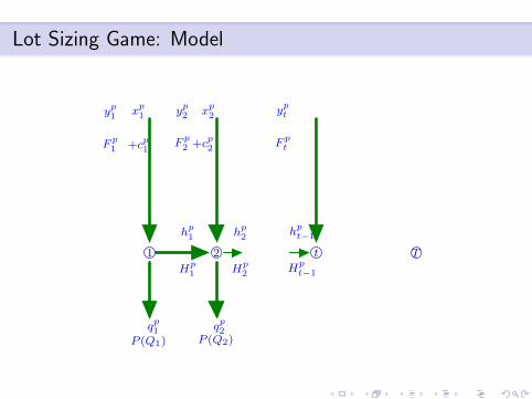
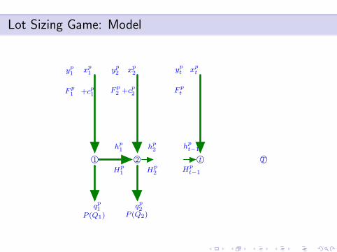
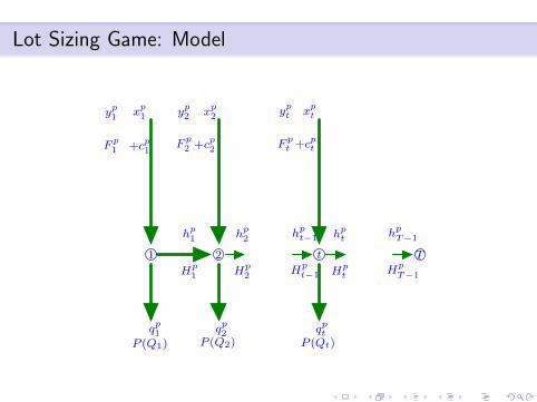
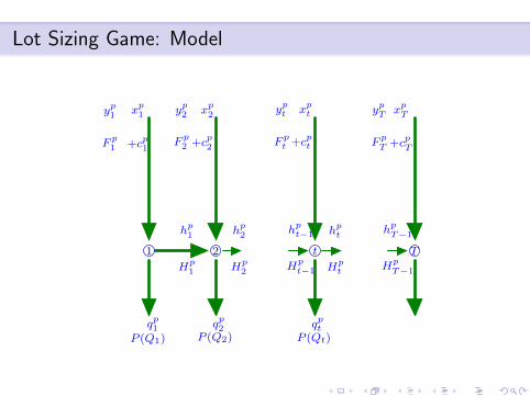
Each player i = 1, 2, . . . ,m solves the following parametric programmingoptimization problem
maxyi,xi,qi,hi
T∑t=1
max(at − bt
m∑j=1
qjt , 0)qit −
T∑t=1
F it y
it −
T∑t=1
Hith
it −
T∑t=1
Citx
it
subject to xit + hi
t−1 = hit + qit for t = 1, . . . , T
0 ≤ xit ≤Myi
t for t = 1, . . . , T
hi0 = hi
T = 0
yit ∈ {0, 1} for t = 1, . . . , T
Margarida Carvalho [email protected] Lot Sizing Games

Motivation Lot Sizing Games
Lot Sizing Game: Formulation
Each player i = 1, 2, . . . ,m solves the following parametric programmingoptimization problem
maxyi,xi,qi,hi
T∑t=1
max(at − bt
m∑j=1
qjt , 0)qit −
T∑t=1
F it y
it −
T∑t=1
Hith
it −
T∑t=1
Citx
it
subject to xit + hi
t−1 = hit + qit for t = 1, . . . , T
0 ≤ xit ≤Myi
t for t = 1, . . . , T
hi0 = hi
T = 0
yit ∈ {0, 1} for t = 1, . . . , T
Margarida Carvalho [email protected] Lot Sizing Games

Motivation Lot Sizing Games
Nash Equilibrium
Definition
A Nash equilibrium (in pure strategies) is a vector of feasible strategies(y1, x1, q1, . . . , ym, xm, qm
), such that for i = 1, 2 . . . ,m:
Πi(y1, x
1, q
1, . . . , y
i, x
i, q
i, . . . , y
m, x
m, q
m)≥ Π
i(y1, x
1, q
1, . . . , y
i, x
i, q
i, . . . , y
m, x
m, q
m)
∀(yi, xi, qi) feasible
In a Nash equilibrium no player has incentive to unilaterally deviate.
Margarida Carvalho [email protected] Lot Sizing Games

Motivation Lot Sizing Games
Lot Sizing Game: should it be reformulated?
Each player i = 1, 2, . . . ,m solves the following parametric programmingoptimization problem
maxyi,xi,qi,hi
T∑t=1
max(at − bt
m∑j=1
qjt , 0)qit −
T∑t=1
F it y
it −
T∑t=1
Hith
it −
T∑t=1
Citx
it
subject to xit + hi
t−1 = hit + qit for t = 1, . . . , T
0 ≤ xit ≤Myi
t for t = 1, . . . , T
hi0 = hi
T = 0
yit ∈ {0, 1} for t = 1, . . . , T
Margarida Carvalho [email protected] Lot Sizing Games

Motivation Lot Sizing Games
Lot Sizing Game: should it be reformulated?
Each player i = 1, 2, . . . ,m solves the following parametric programming optimization problem
maxyi,xi,qi,hi
T∑t=1
max(at − bt
m∑j=1
qjt , 0)q
it −
T∑t=1
Fit y
it −
T∑t=1
Hith
it −
T∑t=1
Citx
it
subject to (yi1, x
i1, q
i1, h
i1) ∈ X1
maxyi,xi,qi,hi
T∑t=2
max(at − bt
m∑j=1
qjt , 0)q
it −
T∑t=2
Fit y
it −
T∑t=2
Hith
it −
T∑t=2
Citx
it
subject to (yi2, x
i2, q
i2, h
i2) ∈ X2
maxyi,xi,qi,hi
T∑t=3
max(at − bt
m∑j=1
qjt , 0)q
it −
T∑t=3
Fit y
it −
T∑t=3
Hith
it −
T∑t=3
Citx
it
subject to (yi3, x
i3, q
i3, h
i3) ∈ X3
. . .
maxyi,xi,qi,hi
max(aT − bT
m∑j=1
qjT, 0)q
iT − F
iT y
iT −H
iT h
iT − C
iT x
iT
subject to (yiT , x
iT , q
iT , h
iT ) ∈ XT
Margarida Carvalho [email protected] Lot Sizing Games

Motivation Lot Sizing Games
Lot Sizing Game: should it be reformulated?Each player i = 1, 2, . . . ,m solves the following parametric programming optimization problem
maxyi,xi,qi,hi
T∑t=1
max(at − bt
m∑j=1
qjt , 0)q
it −
T∑t=1
Fit y
it −
T∑t=1
Hith
it −
T∑t=1
Citx
it
subject to (yi1, x
i1, q
i1, h
i1) ∈ X1
maxyi,xi,qi,hi
T∑t=2
max(at − bt
m∑j=1
qjt , 0)q
it −
T∑t=2
Fit y
it −
T∑t=2
Hith
it −
T∑t=2
Citx
it
subject to (yi2, x
i2, q
i2, h
i2) ∈ X2
maxyi,xi,qi,hi
T∑t=3
max(at − bt
m∑j=1
qjt , 0)q
it −
T∑t=3
Fit y
it −
T∑t=3
Hith
it −
T∑t=3
Citx
it
subject to (yi3, x
i3, q
i3, h
i3) ∈ X3
. . .
maxyi,xi,qi,hi
max(aT − bT
m∑j=1
qjT, 0)q
iT − F
iT y
iT −H
iT h
iT − C
iT x
iT
subject to (yiT , x
iT , q
iT , h
iT ) ∈ XT
In order to compute Nash equilibria the multilevel optimization problem can be relaxed leading to a one leveloptimization programming one.
Margarida Carvalho [email protected] Lot Sizing Games

Motivation Lot Sizing Games
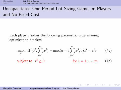
Uncapacitated One Period Lot Sizing Game: m-Playersand No Fixed Cost
Each player i solves the following parametric programmingoptimization problem
maxxi
Πi(xi,m∑
j=1
xj) = max(a− b
m∑
j=1
xj , 0)xi − xici (4a)
subject to xi ≥ 0 for i = 1, . . . ,m (4b)
Margarida Carvalho [email protected] Lot Sizing Games
Motivation Lot Sizing Games
Uncapacitated One Period Lot Sizing Game: m-Playersand No Fixed Cost
Each player i solves the following parametric programmingoptimization problem
maxxi
Πi(xi,m∑
j=1
xj) = max(a− b
m∑
j=1
xj , 0)xi − xici (4a)
subject to xi ≥ 0 for i = 1, . . . ,m (4b)
Margarida Carvalho [email protected] Lot Sizing Games

Motivation Lot Sizing Games
Uncapacitated One Period Lot Sizing Game: m-Playersand No Fixed Cost
Let S ⊆ {1, 2, . . . ,m} be a subset of players producing a strictlypositive quantity.
Margarida Carvalho [email protected] Lot Sizing Games

Motivation Lot Sizing Games
Uncapacitated One Period Lot Sizing Game: m-Playersand No Fixed Cost
Let S ⊆ {1, 2, . . . ,m} be a subset of players producing a strictlypositive quantity.
Optimal quantity to be placed in the market by player i ∈ S is
∂Πi
∂xi= a−2bxi−b
∑
j∈S−{i}
xj−ci = 0⇔ xi =a− b
∑j∈S−{i} x
j − ci
2b.
Margarida Carvalho [email protected] Lot Sizing Games
Motivation Lot Sizing Games
Uncapacitated One Period Lot Sizing Game: m-Playersand No Fixed Cost
Let S ⊆ {1, 2, . . . ,m} be a subset of players producing a strictlypositive quantity.
xi =p(S)− ci
b∀i ∈ S (5a)
xi = 0 ∀i /∈ S. (5b)
where p(S) ≡ a+∑
j∈S cj
|S+1| is the average of the numbers a, {cj}j∈S .
Margarida Carvalho [email protected] Lot Sizing Games

Motivation Lot Sizing Games
Uncapacitated One Period Lot Sizing Game: m-Playersand No Fixed Cost
Let S ⊆ {1, 2, . . . ,m} be a subset of players producing a strictlypositive quantity.
xi =p(S)− ci
b∀i ∈ S (5a)
xi = 0 ∀i /∈ S. (5b)
where p(S) ≡ a+∑
j∈S cj
|S+1| is the average of the numbers a, {cj}j∈S .
p(S) is the resulting market price and the total quantity placed in
the market is∑
i xi = a−p(S)b .
Margarida Carvalho [email protected] Lot Sizing Games

Motivation Lot Sizing Games
Uncapacitated One Period Lot Sizing Game: m-Playersand No Fixed Cost
Using the Nash equilibrium conditions we get
m-Player Lot Sizing Game
INSTANCE Positive integers a, b, c1, c2, . . ., cm−1 and cm.
QUESTION Is there a subset S of {1, 2, . . . ,m} such that
p(S) > ck ∀k ∈ S (6a)
p(S) ≤ ck ∀k /∈ S. (6b)
where p(S) ≡ a+∑
j∈S cj
|S|+1 .
There is always exactly one NE and we can find it in O(m) time (assuming ci
are sorted).
Margarida Carvalho [email protected] Lot Sizing Games

Motivation Lot Sizing Games
Uncapacitated One Period Lot Sizing Game: m-Playersand No Fixed Cost
Using the Nash equilibrium conditions we get
m-Player Lot Sizing Game
INSTANCE Positive integers a, b, c1, c2, . . ., cm−1 and cm.
QUESTION Is there a subset S of {1, 2, . . . ,m} such that
p(S) > ck ∀k ∈ S (6a)
p(S) ≤ ck ∀k /∈ S. (6b)
where p(S) ≡ a+∑
j∈S cj
|S|+1 .
There is always exactly one NE and we can find it in O(m) time (assuming ci
are sorted).Margarida Carvalho [email protected] Lot Sizing Games

Motivation Lot Sizing Games
m-Players and Fixed and Production Costs
Each player i solves the following parametric programmingoptimization problem
maxyi,xi
Πi(xi,
m∑
j=1
xj) = max(a− b
m∑
j=1
xj , 0)xi − F iyi − cixi
subject to 0 ≤ xi ≤Myi for i = 1, . . . ,m
yi ∈ {0, 1} for i = 1, . . . ,m
Margarida Carvalho [email protected] Lot Sizing Games

Motivation Lot Sizing Games
m-Players and Fixed and Production Costs
Let S ⊆ {1, 2, . . . ,m} be a subset of players producing a strictly positivequantity.
Optimal quantity to be placed in the market by player i ∈ S is
xi =(p(S)− ci)+
b
Player k ∈ S - A player k does not have incentive to stop producing if
(p(S)− ck)+
b(p(S)− ck) ≥ F k ⇔ ck +
√F kb ≤ p(S)
Player k /∈ S - A player k does not have incentive to start producing if
(p(S)− ck)
2b
(p(S)− ck)
2≤ F k ⇔ ck + 2
√F kb ≥ p(S)
Margarida Carvalho [email protected] Lot Sizing Games

Motivation Lot Sizing Games
m-Players and Fixed and Production Costs
Using the Nash equilibrium conditions we get
m-Player Lot Sizing Game with fixed and production costs
INSTANCE Positive integers a, b, c1, c2, . . ., cm, F 1, F 2, . . ., Fm.
QUESTION Is there a subset S of {1, 2, . . . ,m} such that
ck +√F kb ≤ p(S) ∀k ∈ S (8a)
ck + 2√F kb ≥ p(S) ∀k /∈ S. (8b)
where p(S) ≡ a+∑
j∈S cj
|S|+1
Margarida Carvalho [email protected] Lot Sizing Games

Motivation Lot Sizing Games
m-Players and Fixed and Production Costs
ck
+√
Fkb ≤ p(S) ∀k ∈ S
ck
+ 2√
Fkb ≥ p(S) ∀k /∈ S.
Computation of one Nash equilibrium
1: Assume that the players are ordered according with√
F1b + c1 ≤√F2b + c2 ≤ . . . ≤
√Fmb + cm.
2: Initialize S ← ∅3: for 1 ≤ k ≤ m do
4: if ck + 2√
Fkb < p(S) then
5: S = S ∪ {k}6: else7: if p(S ∪ {k}) ≥
√Fkb + ck then
8: Arbitrarily decide to set k in S.
9: end if10: end if11: end for12: return S
The algorithm implies that there is always (at least) one NE.
Consider ans instance with ci = 0 and F i = F for i = 1, . . . ,m. Any set S of cardinalityda/(2
√Fb)e − 1 is a NE.
Margarida Carvalho [email protected] Lot Sizing Games

Motivation Lot Sizing Games
m-Players and Fixed and Production Costs
ck
+√
Fkb ≤ p(S) ∀k ∈ S
ck
+ 2√
Fkb ≥ p(S) ∀k /∈ S.
Computation of one Nash equilibrium
1: Assume that the players are ordered according with√F1b + c1 ≤
√F2b + c2 ≤ . . . ≤
√Fmb + cm.
2: Initialize S ← ∅3: for 1 ≤ k ≤ m do
4: if ck + 2√
Fkb < p(S) then
5: S = S ∪ {k}6: else7: if p(S ∪ {k}) ≥
√Fkb + ck then
8: Arbitrarily decide to set k in S.
9: end if10: end if11: end for12: return S
The algorithm implies that there is always (at least) one NE.
Consider ans instance with ci = 0 and F i = F for i = 1, . . . ,m. Any set S of cardinalityda/(2
√Fb)e − 1 is a NE.
Margarida Carvalho [email protected] Lot Sizing Games
Motivation Lot Sizing Games
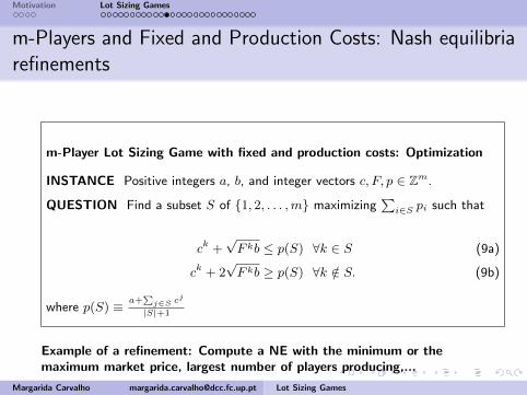
m-Players and Fixed and Production Costs: Nash equilibriarefinements
m-Player Lot Sizing Game with fixed and production costs: Optimization
INSTANCE Positive integers a, b, and integer vectors c, F, p ∈ Zm.
QUESTION Find a subset S of {1, 2, . . . ,m} maximizing∑
i∈S pi such that
ck +√F kb ≤ p(S) ∀k ∈ S (9a)
ck + 2√F kb ≥ p(S) ∀k /∈ S. (9b)
where p(S) ≡ a+∑
j∈S cj
|S|+1
Example of a refinement: Compute a NE with the minimum or themaximum market price, largest number of players producing,...
Margarida Carvalho [email protected] Lot Sizing Games

Motivation Lot Sizing Games
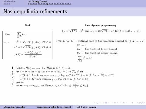
Nash equilibria refinements
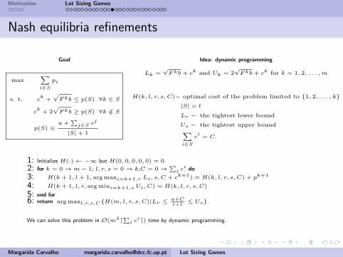
Goal
max∑i∈S
pi
s. t. ck
+√
Fkb ≤ p(S) ∀k ∈ S
ck
+ 2√
Fkb ≥ p(S) ∀k /∈ S
p(S) ≡a +
∑j∈S cj
|S| + 1
Idea: dynamic programming
Lk =√
Fkb + ck and Uk = 2√
Fkb + ck for k = 1, 2, . . . ,m
H(k, l, r, s, C)− optimal cost of the problem limited to {1, 2, . . . , k}|S| = l
Lr − the tightest lower bound
Us − the tightest upper bound∑i∈S
ci
= C.
1: Initialize H(·)← −∞ but H(0, 0, 0, 0, 0) = 0.
2: for k = 0→ m− 1; l, r, s = 0→ k;C = 0→∑i ci do
3: H(k + 1, l + 1, arg maxi=k+1,r Li, s, C + ck+1) = H(k, l, r, s, C) + pk+1
4: H(k + 1, l, r, arg mini=k+1,s Ui, C) = H(k, l, r, s, C)
5: end for6: return arg maxl,r,s,C{H(m, l, r, s, C)|Lr ≤ a+C
l+1≤ Us}.
We can solve this problem in O(m4d∑i cie) time by dynamic programming.
Margarida Carvalho [email protected] Lot Sizing Games

Motivation Lot Sizing Games
Nash equilibria refinements
Goal
max∑i∈S
pi
s. t. ck
+√
Fkb ≤ p(S) ∀k ∈ S
ck
+ 2√
Fkb ≥ p(S) ∀k /∈ S
p(S) ≡a +
∑j∈S cj
|S| + 1
Idea: dynamic programming
Lk =√Fkb + ck and Uk = 2
√Fkb + ck for k = 1, 2, . . . ,m
H(k, l, r, s, C)− optimal cost of the problem limited to {1, 2, . . . , k}|S| = l
Lr − the tightest lower bound
Us − the tightest upper bound∑i∈S
ci
= C.
1: Initialize H(·)← −∞ but H(0, 0, 0, 0, 0) = 0.
2: for k = 0→ m− 1; l, r, s = 0→ k;C = 0→∑i ci do
3: H(k + 1, l + 1, arg maxi=k+1,r Li, s, C + ck+1) = H(k, l, r, s, C) + pk+1
4: H(k + 1, l, r, arg mini=k+1,s Ui, C) = H(k, l, r, s, C)
5: end for6: return arg maxl,r,s,C{H(m, l, r, s, C)|Lr ≤ a+C
l+1≤ Us}.
We can solve this problem in O(m4d∑i cie) time by dynamic programming.
Margarida Carvalho [email protected] Lot Sizing Games

Motivation Lot Sizing Games
T-Periods Lot Sizing Game with Fixed Costs: duopoly
Each player i = 1, 2 solves the following parametric programmingoptimization problem
maxyi,xi,qi,hi
Πi(yi, xi, qi, hi) =
T∑
t=1
max(at − bt(q1t + q2t ), 0)qit −
T∑
t=1
F it y
it
subject to xit + hit−1 = hit + qit for t = 1, . . . , T
0 ≤ xit ≤Myit for t = 1, . . . , T
hi0 = hiT = 0
yit ∈ {0, 1} for t = 1, . . . , T
Margarida Carvalho [email protected] Lot Sizing Games

Motivation Lot Sizing Games
T-Periods Lot Sizing Game with Fixed Costs: duopoly
Lemma
There is always a Player 1’s best reaction to a Player 2’s strategy q2 in whichproduction takes place only once.
Proof.
Assume that given Player 2’s strategy q2 the best reaction of Player 1 involvesproducing in periods 1 ≤ t1 < t2 < . . . < tk ≤ T with k ≥ 2.Let (q1, h1, x1, y1) be the associated Player 1’s strategy. Then, Player 1’s profitis
T∑t=t1
max(at − bt(q2t + q1
t , 0)q1t − Ft1 − Ft2 − . . .− Ftk .
However, Player 1 can maintain or increase her profit by producing only at t1the quantity x1
t1 + x1t1 + . . .+ x1
tk .
Margarida Carvalho [email protected] Lot Sizing Games

Motivation Lot Sizing Games
T-Periods Lot Sizing Game with Fixed Costs: duopoly
Lemma
There is always a Player 1’s best reaction to a Player 2’s strategy q2 in whichproduction takes place only once.
Proof.
Assume that given Player 2’s strategy q2 the best reaction of Player 1 involvesproducing in periods 1 ≤ t1 < t2 < . . . < tk ≤ T with k ≥ 2.
Let (q1, h1, x1, y1) be the associated Player 1’s strategy. Then, Player 1’s profitis
T∑t=t1
max(at − bt(q2t + q1
t , 0)q1t − Ft1 − Ft2 − . . .− Ftk .
However, Player 1 can maintain or increase her profit by producing only at t1the quantity x1
t1 + x1t1 + . . .+ x1
tk .
Margarida Carvalho [email protected] Lot Sizing Games

Motivation Lot Sizing Games
T-Periods Lot Sizing Game with Fixed Costs: duopoly
Lemma
There is always a Player 1’s best reaction to a Player 2’s strategy q2 in whichproduction takes place only once.
Proof.
Assume that given Player 2’s strategy q2 the best reaction of Player 1 involvesproducing in periods 1 ≤ t1 < t2 < . . . < tk ≤ T with k ≥ 2.Let (q1, h1, x1, y1) be the associated Player 1’s strategy. Then, Player 1’s profitis
T∑t=t1
max(at − bt(q2t + q1
t , 0)q1t − Ft1 − Ft2 − . . .− Ftk .
However, Player 1 can maintain or increase her profit by producing only at t1the quantity x1
t1 + x1t1 + . . .+ x1
tk .
Margarida Carvalho [email protected] Lot Sizing Games

Motivation Lot Sizing Games
T-Periods Lot Sizing Game with Fixed Costs: duopoly
Lemma
There is always a Player 1’s best reaction to a Player 2’s strategy q2 in whichproduction takes place only once.
Proof.
Assume that given Player 2’s strategy q2 the best reaction of Player 1 involvesproducing in periods 1 ≤ t1 < t2 < . . . < tk ≤ T with k ≥ 2.Let (q1, h1, x1, y1) be the associated Player 1’s strategy. Then, Player 1’s profitis
T∑t=t1
max(at − bt(q2t + q1
t , 0)q1t − Ft1 − Ft2 − . . .− Ftk .
However, Player 1 can maintain or increase her profit by producing only at t1the quantity x1
t1 + x1t1 + . . .+ x1
tk .
Margarida Carvalho [email protected] Lot Sizing Games

Motivation Lot Sizing Games
T-Periods Lot Sizing Game with Fixed Costs: duopoly
Lemma
Consider that Player 1 only produces at 1 ≤ t1 ≤ T and Player 2 only at1 ≤ t2 ≤ T . Then, Player 1 optimal strategy is
q1t = 0 for t ∈ 1, 2, . . . , t1 − 1
q1t =
at
2btfor t ∈ t1, . . . , t2 − 1, if min(t1, t2) = t1
q1t =
at
3btfor t ∈ max(t1, t2), . . . , T
x1t = 0 for t 6= t1
x1t1 =
T∑t=t1
q1t
Analogous for Player 2.
Margarida Carvalho [email protected] Lot Sizing Games

Motivation Lot Sizing Games
T-Periods Lot Sizing Game with Fixed Costs: duopoly
Corollary
All pure Nash equilibria can be computed in O(T 2) time.
Proof.
Each player has T + 1 strategies to consider. There are (T + 1)2 combinationsof strategies to check the Nash equilibria conditions.
The computational time can be improved!.
Margarida Carvalho [email protected] Lot Sizing Games

Motivation Lot Sizing Games
T-Periods Lot Sizing Game with Fixed Costs: duopoly
Definition
tRp (t) is Player p’s best time to produce when her rivalproduces at time t.
Lemma
tRp (T + 1) ≤ t
Rp (T ) ≤ . . . tRp (1) for p = 1, 2.
Margarida Carvalho [email protected] Lot Sizing Games

Motivation Lot Sizing Games
T-Periods Lot Sizing Game with Fixed Costs: duopoly
Definition
tRp (t) is Player p’s best time to produce when her rivalproduces at time t.
Lemma
tRp (T + 1) ≤ t
Rp (T ) ≤ . . . tRp (1) for p = 1, 2.
Margarida Carvalho [email protected] Lot Sizing Games

Motivation Lot Sizing Games
T-Periods Lot Sizing Game with Fixed Costs: duopoly
Definition
tRp (t) is Player p’s best time to produce when her rivalproduces at time t.
Lemma
tRp (T + 1) ≤ t
Rp (T ) ≤ . . . tRp (1) for p = 1, 2.
Margarida Carvalho [email protected] Lot Sizing Games

Motivation Lot Sizing Games
T-Periods Lot Sizing Game with Fixed Costs: duopolyConsider the time reaction graph GR:
Bipartite graph: R2 = R1 = {1, 2, . . . , T + 1}.
(i, j) is an arc of GR if tR1 (i) = j or tR2 (i) = j.
tRp (T + 1) ≤ t
Rp (T ) ≤ . . . tRp (1) for p = 1, 2.
Traduces in
Lemma (Property 1)
Let (t2, t1) and (t′2, t′1) be arcs of GR with t2, t
′2 ∈ R2 and t1, t
′1 ∈ R1. Then, these arcs cross. The
symmetric result also holds.
Idea: t1 = tR1 (t2) and t′1 = tR1 (t′2).
Assume t2 < t′2,
then tR1 (t2) > tR1 (t′2).
t2 t′2
t1t′1
Margarida Carvalho [email protected] Lot Sizing Games

Motivation Lot Sizing Games
T-Periods Lot Sizing Game with Fixed Costs: duopolyConsider the time reaction graph GR:
Bipartite graph: R2 = R1 = {1, 2, . . . , T + 1}.
(i, j) is an arc of GR if tR1 (i) = j or tR2 (i) = j.
tRp (T + 1) ≤ t
Rp (T ) ≤ . . . tRp (1) for p = 1, 2.
Traduces in
Lemma (Property 1)
Let (t2, t1) and (t′2, t′1) be arcs of GR with t2, t
′2 ∈ R2 and t1, t
′1 ∈ R1. Then, these arcs cross. The
symmetric result also holds.
Idea: t1 = tR1 (t2) and t′1 = tR1 (t′2).
Assume t2 < t′2,
then tR1 (t2) > tR1 (t′2).
t2 t′2
t1
t′1
Margarida Carvalho [email protected] Lot Sizing Games

Motivation Lot Sizing Games
T-Periods Lot Sizing Game with Fixed Costs: duopolyConsider the time reaction graph GR:
Bipartite graph: R2 = R1 = {1, 2, . . . , T + 1}.
(i, j) is an arc of GR if tR1 (i) = j or tR2 (i) = j.
tRp (T + 1) ≤ t
Rp (T ) ≤ . . . tRp (1) for p = 1, 2.
Traduces in
Lemma (Property 1)
Let (t2, t1) and (t′2, t′1) be arcs of GR with t2, t
′2 ∈ R2 and t1, t
′1 ∈ R1. Then, these arcs cross. The
symmetric result also holds.
Idea: t1 = tR1 (t2) and t′1 = tR1 (t′2).
Assume t2 < t′2,
then tR1 (t2) > tR1 (t′2).
t2 t′2
t1t′1
Margarida Carvalho [email protected] Lot Sizing Games

Motivation Lot Sizing Games
T-Periods Lot Sizing Game with Fixed Costs: duopolyConsider the time reaction graph GR:
Bipartite graph: R2 = R1 = {1, 2, . . . , T + 1}.
(i, j) is an arc of GR if tR1 (i) = j or tR2 (i) = j.
tRp (T + 1) ≤ t
Rp (T ) ≤ . . . tRp (1) for p = 1, 2.
Traduces in
Lemma (Property 1)
Let (t2, t1) and (t′2, t′1) be arcs of GR with t2, t
′2 ∈ R2 and t1, t
′1 ∈ R1. Then, these arcs cross. The
symmetric result also holds.
Idea: t1 = tR1 (t2) and t′1 = tR1 (t′2).
Assume t2 < t′2,
then tR1 (t2) > tR1 (t′2).
t2 t′2
t1t′1
Margarida Carvalho [email protected] Lot Sizing Games
Motivation Lot Sizing Games
T-Periods Lot Sizing Game with Fixed Costs: duopoly
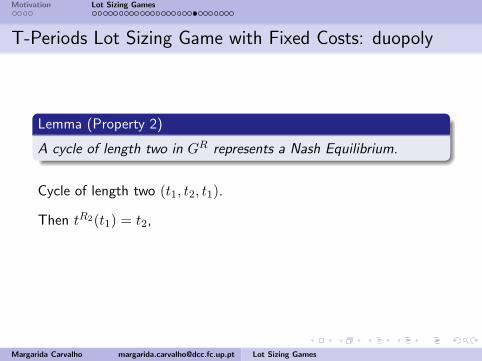
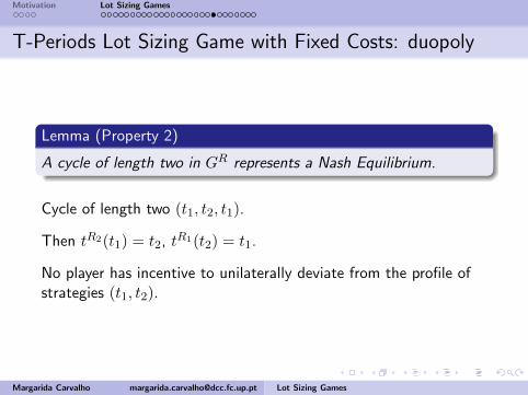
Lemma (Property 2)
A cycle of length two in GR represents a Nash Equilibrium.
Cycle of length two (t1, t2, t1).
Then tR2(t1) = t2, tR1(t2) = t1.
No player has incentive to unilaterally deviate from the profile ofstrategies (t1, t2).
Margarida Carvalho [email protected] Lot Sizing Games

Motivation Lot Sizing Games
T-Periods Lot Sizing Game with Fixed Costs: duopoly
Lemma (Property 2)
A cycle of length two in GR represents a Nash Equilibrium.
Cycle of length two (t1, t2, t1).
Then tR2(t1) = t2, tR1(t2) = t1.
No player has incentive to unilaterally deviate from the profile ofstrategies (t1, t2).
Margarida Carvalho [email protected] Lot Sizing Games
Motivation Lot Sizing Games
T-Periods Lot Sizing Game with Fixed Costs: duopoly
Lemma (Property 2)
A cycle of length two in GR represents a Nash Equilibrium.
Cycle of length two (t1, t2, t1).
Then tR2(t1) = t2,
tR1(t2) = t1.
No player has incentive to unilaterally deviate from the profile ofstrategies (t1, t2).
Margarida Carvalho [email protected] Lot Sizing Games

Motivation Lot Sizing Games
T-Periods Lot Sizing Game with Fixed Costs: duopoly
Lemma (Property 2)
A cycle of length two in GR represents a Nash Equilibrium.
Cycle of length two (t1, t2, t1).
Then tR2(t1) = t2, tR1(t2) = t1.
No player has incentive to unilaterally deviate from the profile ofstrategies (t1, t2).
Margarida Carvalho [email protected] Lot Sizing Games
Motivation Lot Sizing Games
T-Periods Lot Sizing Game with Fixed Costs: duopoly
Lemma (Property 2)
A cycle of length two in GR represents a Nash Equilibrium.
Cycle of length two (t1, t2, t1).
Then tR2(t1) = t2, tR1(t2) = t1.
No player has incentive to unilaterally deviate from the profile ofstrategies (t1, t2).
Margarida Carvalho [email protected] Lot Sizing Games

Motivation Lot Sizing Games
T-Periods Lot Sizing Game with Fixed Costs: duopoly
Lemma (Property 3)
Let (t1, t2), (t2, t′1) and (t′1, t
′2) be arcs of GR with t2, t
′2 ∈ R2 and t1, t
′1 ∈ R1. If t1 ≤ t′1 ≤ t′2 ≤ t2
then, (t′1, t2) is a NE.
1 . . . t1 t′1 . . . T T + 1
1 . . . t′2 t2 . . . T T + 1
−F 2t2 +
a2t2
9bt2
a2t2
9bt2
a2T
9bTduopoly−F 2
t′2+
a2t′2
9bt′2
Π2(t1, t2) ≥ Π2(t1, t′2) and Π2(t′1, t
′2) ≥ Π2(t′1, t2)
Π2(t1, t2) = Π2(t′1, t2)
⇒ Π2(t1, t2) = Π2(t1, t′2) = Π2(t′1, t
′2) = Π2(t′1, t2)⇒ tR2 (t1) = tR2 (t′1) = t2 ⇒ NE: (t′1, t2)
Π2(t′1, t′2) = Π2(t1, t
′2)⇒ tR2 (t′1) = tR2 (t1) = t′2
Margarida Carvalho [email protected] Lot Sizing Games

Motivation Lot Sizing Games
T-Periods Lot Sizing Game with Fixed Costs: duopoly
Lemma (Property 3)
Let (t1, t2), (t2, t′1) and (t′1, t
′2) be arcs of GR with t2, t
′2 ∈ R2 and t1, t
′1 ∈ R1. If t1 ≤ t′1 ≤ t′2 ≤ t2
then, (t′1, t2) is a NE.
1 . . . t1 t′1 . . . T T + 1
1 . . . t′2 t2 . . . T T + 1
−F 2t2 +
a2t2
9bt2
a2t2
9bt2
a2T
9bTduopoly−F 2
t′2+
a2t′2
9bt′2
Π2(t1, t2) ≥ Π2(t1, t′2)
and Π2(t′1, t′2) ≥ Π2(t′1, t2)
Π2(t1, t2) = Π2(t′1, t2)
⇒ Π2(t1, t2) = Π2(t1, t′2) = Π2(t′1, t
′2) = Π2(t′1, t2)⇒ tR2 (t1) = tR2 (t′1) = t2 ⇒ NE: (t′1, t2)
Π2(t′1, t′2) = Π2(t1, t
′2)⇒ tR2 (t′1) = tR2 (t1) = t′2
Margarida Carvalho [email protected] Lot Sizing Games

Motivation Lot Sizing Games
T-Periods Lot Sizing Game with Fixed Costs: duopoly
Lemma (Property 3)
Let (t1, t2), (t2, t′1) and (t′1, t
′2) be arcs of GR with t2, t
′2 ∈ R2 and t1, t
′1 ∈ R1. If t1 ≤ t′1 ≤ t′2 ≤ t2
then, (t′1, t2) is a NE.
1 . . . t1 t′1 . . . T T + 1
1 . . . t′2 t2 . . . T T + 1
−F 2t2 +
a2t2
9bt2
a2t2
9bt2
a2T
9bTduopoly−F 2
t′2+
a2t′2
9bt′2
Π2(t1, t2) ≥ Π2(t1, t′2) and Π2(t′1, t
′2) ≥ Π2(t′1, t2)
Π2(t1, t2) = Π2(t′1, t2)
⇒ Π2(t1, t2) = Π2(t1, t′2) = Π2(t′1, t
′2) = Π2(t′1, t2)⇒ tR2 (t1) = tR2 (t′1) = t2 ⇒ NE: (t′1, t2)
Π2(t′1, t′2) = Π2(t1, t
′2)⇒ tR2 (t′1) = tR2 (t1) = t′2
Margarida Carvalho [email protected] Lot Sizing Games

Motivation Lot Sizing Games
T-Periods Lot Sizing Game with Fixed Costs: duopoly
Lemma (Property 3)
Let (t1, t2), (t2, t′1) and (t′1, t
′2) be arcs of GR with t2, t
′2 ∈ R2 and t1, t
′1 ∈ R1. If t1 ≤ t′1 ≤ t′2 ≤ t2
then, (t′1, t2) is a NE.
1 . . . t1 t′1 . . . T T + 1
1 . . . t′2 t2 . . . T T + 1
−F 2t2 +
a2t2
9bt2
a2t2
9bt2
a2T
9bTduopoly
−F 2t′2
+a2t′2
9bt′2
Π2(t1, t2) ≥ Π2(t1, t′2) and Π2(t′1, t
′2) ≥ Π2(t′1, t2)
Π2(t1, t2) = Π2(t′1, t2)
⇒ Π2(t1, t2) = Π2(t1, t′2) = Π2(t′1, t
′2) = Π2(t′1, t2)⇒ tR2 (t1) = tR2 (t′1) = t2
⇒ NE: (t′1, t2)
Π2(t′1, t′2) = Π2(t1, t
′2)⇒ tR2 (t′1) = tR2 (t1) = t′2
Margarida Carvalho [email protected] Lot Sizing Games

Motivation Lot Sizing Games
T-Periods Lot Sizing Game with Fixed Costs: duopoly
Lemma (Property 3)
Let (t1, t2), (t2, t′1) and (t′1, t
′2) be arcs of GR with t2, t
′2 ∈ R2 and t1, t
′1 ∈ R1. If t1 ≤ t′1 ≤ t′2 ≤ t2
then, (t′1, t2) is a NE.
1 . . . t1 t′1 . . . T T + 1
1 . . . t′2 t2 . . . T T + 1
−F 2t2 +
a2t2
9bt2
a2t2
9bt2
a2T
9bTduopoly
−F 2t′2
+a2t′2
9bt′2
Π2(t1, t2) ≥ Π2(t1, t′2) and Π2(t′1, t
′2) ≥ Π2(t′1, t2)
Π2(t1, t2) = Π2(t′1, t2)
⇒ Π2(t1, t2) = Π2(t1, t′2) = Π2(t′1, t
′2) = Π2(t′1, t2)⇒ tR2 (t1) = tR2 (t′1) = t2 ⇒ NE: (t′1, t2)
Π2(t′1, t′2) = Π2(t1, t
′2)⇒ tR2 (t′1) = tR2 (t1) = t′2
Margarida Carvalho [email protected] Lot Sizing Games

Motivation Lot Sizing Games
T-Periods Lot Sizing Game with Fixed Costs: duopoly
Lemma (Property 3)
Let (t1, t2), (t2, t′1) and (t′1, t
′2) be arcs of GR with t2, t
′2 ∈ R2 and t1, t
′1 ∈ R1. If t1 ≤ t′1 ≤ t′2 ≤ t2
then, (t′1, t2) is a NE.
1 . . . t1 t′1 . . . T T + 1
1 . . . t′2 t2 . . . T T + 1
−F 2t2 +
a2t2
9bt2
a2t2
9bt2
a2T
9bTduopoly−F 2
t′2+
a2t′2
9bt′2
Π2(t1, t2) ≥ Π2(t1, t′2) and Π2(t′1, t
′2) ≥ Π2(t′1, t2)
Π2(t1, t2) = Π2(t′1, t2)
⇒ Π2(t1, t2) = Π2(t1, t′2) = Π2(t′1, t
′2) = Π2(t′1, t2)⇒ tR2 (t1) = tR2 (t′1) = t2 ⇒ NE: (t′1, t2)
Π2(t′1, t′2) = Π2(t1, t
′2)
⇒ tR2 (t′1) = tR2 (t1) = t′2
Margarida Carvalho [email protected] Lot Sizing Games

Motivation Lot Sizing Games
T-Periods Lot Sizing Game with Fixed Costs: duopoly
Lemma (Property 3)
Let (t1, t2), (t2, t′1) and (t′1, t
′2) be arcs of GR with t2, t
′2 ∈ R2 and t1, t
′1 ∈ R1. If t1 ≤ t′1 ≤ t′2 ≤ t2
then, (t′1, t2) is a NE.
1 . . . t1 t′1 . . . T T + 1
1 . . . t′2 t2 . . . T T + 1
−F 2t2 +
a2t2
9bt2
a2t2
9bt2
a2T
9bTduopoly−F 2
t′2+
a2t′2
9bt′2
Π2(t1, t2) ≥ Π2(t1, t′2) and Π2(t′1, t
′2) ≥ Π2(t′1, t2)
Π2(t1, t2) = Π2(t′1, t2)
⇒ Π2(t1, t2) = Π2(t1, t′2) = Π2(t′1, t
′2) = Π2(t′1, t2)⇒ tR2 (t1) = tR2 (t′1) = t2 ⇒ NE: (t′1, t2)
Π2(t′1, t′2) = Π2(t1, t
′2)⇒ tR2 (t′1) = tR2 (t1) = t′2
Margarida Carvalho [email protected] Lot Sizing Games

Motivation Lot Sizing Games
T-Periods Lot Sizing Game with Fixed Costs: duopoly
Lemma (Property 3)
Let (t1, t2), (t2, t′1) and (t′1, t
′2) be arcs of GR with t2, t
′2 ∈ R2 and t1, t
′1 ∈ R1. If t1 ≤ t′1 ≤ t′2 ≤ t2
then, (t′1, t2) is a NE.
1 . . . t1 t′1 . . . T T + 1
1 . . . t′2 t2 . . . T T + 1
−F 2t2 +
a2t2
9bt2
a2t2
9bt2
a2T
9bTduopoly−F 2
t′2+
a2t′2
9bt′2
Π2(t1, t2) ≥ Π2(t1, t′2) and Π2(t′1, t
′2) ≥ Π2(t′1, t2)
Π2(t1, t2) = Π2(t′1, t2)
⇒ Π2(t1, t2) = Π2(t1, t′2) = Π2(t′1, t
′2) = Π2(t′1, t2)⇒ tR2 (t1) = tR2 (t′1) = t2 ⇒ NE: (t′1, t2)
Π2(t′1, t′2) = Π2(t1, t
′2)⇒ tR2 (t′1) = tR2 (t1) = t′2
Margarida Carvalho [email protected] Lot Sizing Games

Motivation Lot Sizing Games
T-Periods Lot Sizing Game with Fixed Costs: duopoly
Corollary
A Nash equilibrium is found after following at most a path oflength 5 in GR. In particular, there is always a Nash equilibrium.
t1 . . . t′1 . . . t1
t2 . . . t′2 . . . t2
Margarida Carvalho [email protected] Lot Sizing Games
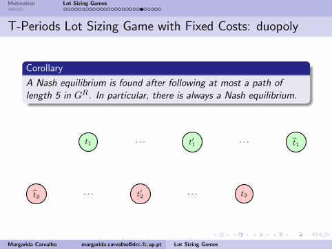
Motivation Lot Sizing Games
T-Periods Lot Sizing Game with Fixed Costs: duopoly
Corollary
A Nash equilibrium is found after following at most a path oflength 5 in GR. In particular, there is always a Nash equilibrium.
t1 . . . t′1 . . . t1
t2 . . . t′2 . . . t2
Margarida Carvalho [email protected] Lot Sizing Games

Motivation Lot Sizing Games
T-Periods Lot Sizing Game with Fixed Costs: duopoly
Margarida Carvalho [email protected] Lot Sizing Games

T-Periods Lot Sizing Game with Fixed Costs: duopoly
Theorem
For p = 1, 2
tRp(t) ∈ {tRp(T + 1), tRp(1)} ∀t ∈ {1, 2, . . . , T, T + 1}.
Moreover, (tR1(1), tR2(T + 1)) and (tR1(T + 1), tR2(1)) are the onlycandidates to be Nash equilibria.
1 T + 1T
1 T + 1T
tR1 (1)tR1 (T + 1)
t2
tR1 (t2)

T-Periods Lot Sizing Game with Fixed Costs: duopoly
Theorem
For p = 1, 2
tRp(t) ∈ {tRp(T + 1), tRp(1)} ∀t ∈ {1, 2, . . . , T, T + 1}.
Moreover, (tR1(1), tR2(T + 1)) and (tR1(T + 1), tR2(1)) are the onlycandidates to be Nash equilibria.
1 T + 1T
1 T + 1T
tR1 (1)
tR1 (T + 1)
t2
tR1 (t2)

T-Periods Lot Sizing Game with Fixed Costs: duopoly
Theorem
For p = 1, 2
tRp(t) ∈ {tRp(T + 1), tRp(1)} ∀t ∈ {1, 2, . . . , T, T + 1}.
Moreover, (tR1(1), tR2(T + 1)) and (tR1(T + 1), tR2(1)) are the onlycandidates to be Nash equilibria.
1 T + 1T
1 T + 1T
tR1 (1)tR1 (T + 1)
t2
tR1 (t2)

T-Periods Lot Sizing Game with Fixed Costs: duopoly
Theorem
For p = 1, 2
tRp(t) ∈ {tRp(T + 1), tRp(1)} ∀t ∈ {1, 2, . . . , T, T + 1}.
Moreover, (tR1(1), tR2(T + 1)) and (tR1(T + 1), tR2(1)) are the onlycandidates to be Nash equilibria.
1 T + 1T
1 T + 1T
tR1 (1)tR1 (T + 1)
t2
tR1 (t2)

T-Periods Lot Sizing Game with Fixed Costs: duopoly
Theorem
For p = 1, 2
tRp(t) ∈ {tRp(T + 1), tRp(1)} ∀t ∈ {1, 2, . . . , T, T + 1}.
Moreover, (tR1(1), tR2(T + 1)) and (tR1(T + 1), tR2(1)) are the onlycandidates to be Nash equilibria.
1 T + 1T
1 T + 1T
tR1 (1)tR1 (T + 1)
t2
tR1 (t2)

T-Periods Lot Sizing Game with Fixed Costs: duopoly
Theorem
For p = 1, 2
tRp(t) ∈ {tRp(T + 1), tRp(1)} ∀t ∈ {1, 2, . . . , T, T + 1}.
Moreover, (tR1(1), tR2(T + 1)) and (tR1(T + 1), tR2(1)) are the onlycandidates to be Nash equilibria.
1 T + 1T
1 T + 1T
tR1 (1)tR1 (T + 1)
t2
tR1 (t2)

Motivation Lot Sizing Games
T-Periods Lot Sizing Game with Fixed Costs: oligopoly
It is easy to generalize the previous ideas for m > 2.
All pure Nash equilibria can be computed in polynomial timefor a fixed number of players, more precisely, in O(Tm) time.Idea: Each player only has to decide one period to produce.
All pure Nash equilibria can be computed in polynomial timefor a fixed number of periods, more precisely, in O(mT ) time.Idea:
Define Si as the set of players producing in period i.For the point of view of player k, only the fixed costs of k andthe sizes of the sets Si matter.We can enumerate all possible sizes for these partitions:O(mT ) time.Once these sizes are fixed, assigning the players to the sets Si
is easy - a transportation problem.
Margarida Carvalho [email protected] Lot Sizing Games

Motivation Lot Sizing Games
T-Periods Lot Sizing Game with Fixed Costs: oligopoly
It is easy to generalize the previous ideas for m > 2.
All pure Nash equilibria can be computed in polynomial timefor a fixed number of players, more precisely, in O(Tm) time.Idea: Each player only has to decide one period to produce.
All pure Nash equilibria can be computed in polynomial timefor a fixed number of periods, more precisely, in O(mT ) time.Idea:
Define Si as the set of players producing in period i.
For the point of view of player k, only the fixed costs of k andthe sizes of the sets Si matter.We can enumerate all possible sizes for these partitions:O(mT ) time.Once these sizes are fixed, assigning the players to the sets Si
is easy - a transportation problem.
Margarida Carvalho [email protected] Lot Sizing Games

Motivation Lot Sizing Games
T-Periods Lot Sizing Game with Fixed Costs: oligopoly
It is easy to generalize the previous ideas for m > 2.
All pure Nash equilibria can be computed in polynomial timefor a fixed number of players, more precisely, in O(Tm) time.Idea: Each player only has to decide one period to produce.
All pure Nash equilibria can be computed in polynomial timefor a fixed number of periods, more precisely, in O(mT ) time.Idea:
Define Si as the set of players producing in period i.For the point of view of player k, only the fixed costs of k andthe sizes of the sets Si matter.
We can enumerate all possible sizes for these partitions:O(mT ) time.Once these sizes are fixed, assigning the players to the sets Si
is easy - a transportation problem.
Margarida Carvalho [email protected] Lot Sizing Games

Motivation Lot Sizing Games
T-Periods Lot Sizing Game with Fixed Costs: oligopoly
It is easy to generalize the previous ideas for m > 2.
All pure Nash equilibria can be computed in polynomial timefor a fixed number of players, more precisely, in O(Tm) time.Idea: Each player only has to decide one period to produce.
All pure Nash equilibria can be computed in polynomial timefor a fixed number of periods, more precisely, in O(mT ) time.Idea:
Define Si as the set of players producing in period i.For the point of view of player k, only the fixed costs of k andthe sizes of the sets Si matter.We can enumerate all possible sizes for these partitions:O(mT ) time.
Once these sizes are fixed, assigning the players to the sets Si
is easy - a transportation problem.
Margarida Carvalho [email protected] Lot Sizing Games

Motivation Lot Sizing Games
T-Periods Lot Sizing Game with Fixed Costs: oligopoly
It is easy to generalize the previous ideas for m > 2.
All pure Nash equilibria can be computed in polynomial timefor a fixed number of players, more precisely, in O(Tm) time.Idea: Each player only has to decide one period to produce.
All pure Nash equilibria can be computed in polynomial timefor a fixed number of periods, more precisely, in O(mT ) time.Idea:
Define Si as the set of players producing in period i.For the point of view of player k, only the fixed costs of k andthe sizes of the sets Si matter.We can enumerate all possible sizes for these partitions:O(mT ) time.Once these sizes are fixed, assigning the players to the sets Si
is easy - a transportation problem.
Margarida Carvalho [email protected] Lot Sizing Games

Motivation Lot Sizing Games
T-Periods Lot Sizing Game with Fixed Costs: oligopoly
Theorem
For p = 1, 2, . . . ,m and for all feasible partitionsS−p = (|S1|, |S2|, . . . , |ST |) of the set of all players except p:
tRp(S−p) ∈ {tRp(0, 0, . . . , 0), tRp(1, 0, . . . , 0), . . . , tRp(m− 1, 0. . . . , 0)}.
There are mm candidates to be Nash equilibria...
Margarida Carvalho [email protected] Lot Sizing Games
Motivation Lot Sizing Games
Conclusion and Future work
1-Period Lot sizing game:
F Existence of a pure Nash equilibrium.
F A pure Nash equilibrium can be computed in polynomialtime.
F Current work: Is it “NP -complete” to compute a Nashequilibrium optimizing a certain function? What is the economicmeaning of ck +
√F kb?
T-Period Lot sizing game with fixed costs:
F Computation in polynomial time of all equilibria for the2-players game.
F Current work: Can we compute in polynomial time (onthe number of players and number of periods) a Nash equilibrium?
Margarida Carvalho [email protected] Lot Sizing Games
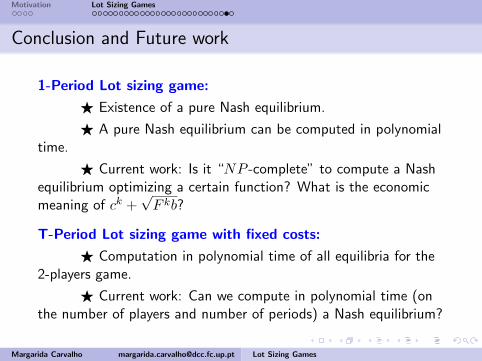

Motivation Lot Sizing Games
Acknowledgments
I am grateful to GEMAC - Gabinete de Estatıstica, Modelacao e Aplicacoes Computacionais - for supporting myparticipation in 5th Porto Meeting on MATHEMATICS for INDUSTRY.
Margarida Carvalho [email protected] Lot Sizing Games