Embed Size (px)
Citation preview
Period Decompositions for the Capacitated Lot
Sizing Problem with Setup Times
Silvio Alexandre de Araujo Departamento de Matemática Aplicada, Universidade Estadual Paulista, São José do Rio Preto SP, 15054-000, Brazil
Bert De Reyck Department of Management Science and Innovation, University College London, WC1E 6BT, UK
Zeger Degraeve Melbourne Business School, University of Melbourne, Carlton VIC 3053, [email protected]
Department of Mamagement Science and Operations, London Business School, Regents Park, London NW1 4SA, UK
Ioannis Fragkos Department of Management Science and Innovation, University College London, WC1E 6BT, UK
Raf Jans HEC Montréal, H3T 2A7 QC, Canada
We study the Capacitated Lot Sizing Problem with Setup Times (CLST). Based on two strong
reformulations of the problem, we present a transformed reformulation and valid inequalities that
speed up column generation and Lagrange relaxation. We demonstrate computationally how both
ideas enhance the performance of our algorithm and show theoretically how they are related to dual
space reduction techniques. We compare several solution methods, and propose a new efficient
hybrid scheme that combines column generation and Lagrange relaxation in a novel way.
Computational experiments show that the proposed solution method for finding lower bounds is
competitive with textbook approaches and state-of-the-art approaches found in the literature. Finally,
a branch-and-price based heuristic is designed and computational results are reported. The heuristic
scheme compares favorably or outperforms other approaches.
Key words: Lot Sizing; Column Generation; Lagrange Relaxation; Branch-and-Price; Heuristics.
History: Submitted, August 2013.
1. Introduction
Lot sizing problems have been studied extensively by the operations research community in the past
five decades. Despite the vast progress of mixed integer programming theory and software, many lot
sizing problems remain computationally challenging to solve in practice. In this paper we study a
classical lot sizing problem, namely the Multi-Item Capacitated Lot Sizing Problem with Setup
Times (CLST). Given a discrete time horizon, the objective of CLST is to find a minimum cost
production plan that satisfies the demand for all items and respects the per period capacity
constraints. A setup operation is necessary whenever a positive amount is produced in a period. Such
a setup entails a cost and consumes capacity. Morever, production is done on a single-machine that
can produce many items in any given period, and no dependencies among items exist other than the
single-machine capacity restriction. CLST is classified as a multi item, single machine, single level,
big bucket capacitated lot sizing problem. In spite of the simple problem statement and its simple
formulation, CLST instances can be computationally challenging even for modern mixed integer
programming software. In particular, obtaining tight lower bounds and good feasible solutions
requires considerable effort, if at all possible, even for instances with a few hundred integer
variables.
The aim of this paper is to design a fast heuristic procedure for CLST that provides good
solutions and a strong lower bound used to assess the solution quality. Period Danzig-Wolfe
decompositions of two network reformulations of CLST are proposed. The main advantage of the
proposed decompositions is that they provide a lower bound which is stronger than these of the
standard and network formulations. The potential downside is their computational tractability: when
computed with column generation, the already large number of variables of the network formulations
and their inherent degeneracy could lead to long solution times for the restricted master (RM)
programs, and only minor bound improvements per iteration. Although there exists limited
computational experience with decompositions of extended formulations on this problem, evidence
suggests that simplex-based solvers do not exhibit good convergence behavior (Jans and Degraeve
2004). We propose a novel, considerably faster subgradient-based hybrid scheme that combines
Lagrange relaxation and column generation. This scheme gives valid lower bounds of excellent
quality and outperforms pure simplex-based column generation, Lagrange relaxation and
subgradient-based column generation (in which the RM programs are solved with subgradient
optimization). Further, we enhance the performance of our algorithm by utilizing two new dual space
reduction techniques. First, we show how a primal space reformulation can lead to improved
performance of dual based algorithms during column generation. Second, we employ a class of valid
inequalities introduced by Wolsey (1989) in the context of single-item problems with start-up costs
and show how this corresponds to adding dual optimal inequalities in the dual space of the RM
program (Ben Amor et al. 2007). The new subproblems remain tractable and the performance of the
hybrid column generation scheme is improved further.
The new hybrid scheme is embedded in a heuristic branch-and-price framework, designed
specifically to obtain good feasible solutions fast. To achieve this, we recover a primal solution of
the RM using the volume algorithm of Barahona and Anbil (2000) and branch on the resulting
fractional setup variables. Moreover, we integrate in a customized fashion recent MIP-based
heuristic approaches, such as relaxation induced neighborhoods and selective dives (Danna et al.
2005), with established ones such as the forward/backward smoothing heuristic of Trigeiro et al.
(1989). Extensive computational experiments show that the branch-and-price heuristic performs very
well against other competitive approaches.
The remainer of this paper is organised as follows. Section 2 provides a brief literature
review. Section 3 describes CLST formulations, and Section 4 their Dantzig-Wolfe decompositions.
Section 5 describes customized procedures for solving the subproblems. Section 6 describes the
hybrid scheme and Section 7 the branch-and-price heuristic. Finally, Section 8 presents
computational results and Section 9 concludes with comments and directions for future research.
2. Literature Review
The literature on capacitated lot sizing problems is vast. A broad categorization would distinguish
research related to exact and heuristic methods. We review both streams of literature, as our
approach utilizes exact methods but also constructs heuristic solutions.
With respect to the more recent research on exact approaches, Van Vyve and Wolsey (2006)
suggest an approximate extended formulation based on the network reformulation of Eppen and
Martin (1987) that uses a single parameter to control the trade off between the number of variables
and the lower bound strength. They show that selecting small values of that parameter is sufficient to
solve hard problems, especially when a redundant row that facilitates the solver to generate cuts is
added in the formulation. Degraeve and Jans (2007) discuss the structural deficiency of the
decomposition proposed by Manne (1958) which only allows the computation of a lower bound for
the problem. Furthermore they show the correct implementation of the Dantzig-Wolfe decomposition
principle for CLST and develop a branch-and-price algorithm. Pimentel et al. (2010) propose three
Dantzig-Wolfe decompositions of the standard formulation of CLST, and compare the performance
of the corresponding branch-and-price algorithms. Specifically, they describe and compare the item,
period and simultaneous item and period decompositions. Belvaux and Wolsey (2000) developed
BC-PROD, a specialized branch-and-cut system for generic lot sizing problems. Some of the
cornerstone work that is less recent are the variable redefinition approach of Eppen and Martin
(1987), the use of valid inequalities (Barany et al. 1984) and the simple plant location reformulation
of Krarup and Bilde (1977). Recently, many authors (Alfieri et al. 2002, Pochet and Van Vyve 2004,
Denizel et al. 2008 and Süral et al. 2009) have used such alternative formulations with stronger linear
relaxations for the CLSP. Finally, Miller et al. (2000b, 2003) also derive strong valid inequalities
from simplified models, which are single-period relaxations with preceding inventory. The single
period models contain the capacity constraint and the demand constraints for multiple items taking
into account only the preceding inventory level.
Heuristic approaches have also received considerable attention. The seminal paper of Trigeiro
et al. (1989) proposed a item Lagrange relaxation and presented a smoothing heuristic (TTM) that
was able to find good feasible solutions quickly. Heuristics that use several iterations of solving a
reduced problem such as relax-and-fix and relax-and-optimize, have been successfully used by a
number of researchers (Pochet and Wolsey 2005, Stadtler 2006, Helber and Sahling 2010). Süral et
al. (2009) designed a Lagrange relaxation based heuristic that outperforms TTM for problems
without setup costs. Other recent heuristic approaches include among others, the cross entropy-
Lagrange hybrid algorithm of Caserta and Rico (2009), the adaptive large neighbourhood search
algorithm of Müller et al. (2012), the LP-based heuristic and curtailed branch-and-bound of Denizel
and Süral (2006) and the iterative production estimate (IPE) heuristic of Pochet and Van Vyve
(2004). A notable recent approach is that of Tempelmeier (2011), who uses a set partitioning
approximation and a column generation-based heuristic to solve a multi-item capacitated model with
random demands and a fill rate constraint. A very comprehensive review of heuristic approaches can
be found in Buschkühl et al. (2010).
Relevant to the current work is also the decomposition approach proposed in Jans and
Degraeve (2004). The authors propose a period decomposition of a strong reformulation proposed in
Eppen and Martin (1987). They obtain improved lower bounds, but their computational experiments
show that standard computation schemes may be very time consuming for hard problems. Finally,
Fiorotto and de Araujo (2014) build upon and extend the Lagrangian relaxation presented in Jans and
Degraeve (2004) by developing a heuristic for the capacitated lot sizing problem with parallel
machines.
The main contributions of the present work are (a) the development and comparison of two
period Dantzig-Wolfe network reformulations for CLST; (b) the development of a methodology that
circumvents the computational difficulties of extended formulations through the design of a
stabilization algorithm, and the use of problem-specific inequalities in the customized algorithm that
solves the subproblems; (c) the development of a state-of-the-art branch-and-price heuristic that
integrates and customizes several recent advances such as the volume algorithm (Barahona and
Anbil 2000), relaxation induced neighbourhoods and selected dives (Danna et al. 2005) and finally,
(d) the presentation of computational results that suggest the competitiveness of the proposed scheme
against other approaches.
The next section gives an overview of several formulations that are used throughout the paper.
3. Formulations for the Capacitated Lot Sizing Problem
In this section we present different formulations for the capacitated lot sizing problem: the regular
formulation (CL); the shortest path formulation (SP) proposed in Eppen and Martin (1987); a
transformed shortest path formulation (SPt); the facility location formulation (FL) studied in Krarup
and Bilde (1977); and the facility location formulation with precedence constraints (FLp).
3.1. The Regular Formulation (CL)
The regular formulation for the Capacitated Lot Sizing Problem with Setup Times is described by
the following sets, parameters and decisions variables (Trigeiro et al. 1987).
Sets:
I : set of items, = {1,…, |I|},
T : set of time periods, = {1,…, |T|}.
Parameters:
itd : demand of item i in period t, Ii , t T
itksd : sum of demand of item i, from period t until k, Ii , t, k T: k t
ithc : unit holding cost for item i in period t, Ii , t T
itsc : setup cost for item i in period t, Ii , t T
itvc : variable production cost for item i in period t, Ii , t T
ifc : unit cost for initial inventory for item i, Ii
itst : setup time for item i in period t, Ii , t T
itvt : variable production time for item i in period t, Ii , t T
tcap : time capacity in period t. t T
Decision variables:
itx : production quantity of item i in period t, Ii , t T
ity = 1 if setup for item i in period t, = 0 otherwise, Ii , t T
its : inventory for item i at the end of period t, Ii , t T
0is : amount of initial inventory for item i. Ii
The mathematical formulation of CLST is then as follows:

Ii Tt
itititititit
Ii
ii shcxvcyscsfc 0min CL (1)
s.t. itititti sdxs 1, i I, t T (2)
t
Ii
itititit capxvtyst
t T (3)
itTit
it
ittit ysd
vt
stcapx
||,min Ii , t T (4)
}1,0{ity , 0itx , 0its , 00 is , 0|| Tis Ii , t T (5)
The objective function (1) minimizes the setup cost, the variable production cost, the
inventory holding cost and initial inventory cost. Constraints (2) are the demand constraints:
inventory carried over from the previous period and production in the current period can be used to
satisfy current demand and build up inventory. As in Vanderbeck (1998), we deal with possible
infeasible problems by allowing for initial inventory (si0) which is available in the first period at a
large cost, fci. There is no setup required for initial inventory. Next, there is a constraint on the
available capacity in each period (3). Constraint (4) forces the setup variable to one if any production
takes place in that period. Finally, we have the non-negativity and integrality constraints (5) and the
ending inventory is set to zero.
3.2. The Shortest Path Formulation (SP)
Next, model (1)-(5) is reformulated using the variable redefinition approach of Eppen and Martin
(1987). Define the following parameters:
itkcv : total production and holding cost for producing item i in period t to satisfy
demand for the periods t until k,
k
1ts
1s
tu
isiuitkititk dhcsdvccv ,
itci : total production and holding cost for initial inventory for item i to satisfy
demand from period 1 up to period t,
t
2s
1s
1u
isiut1iiit dhcsdfcci .
We also have the following new variables:
itkz : fraction of the production plan for item i where production in period t
satisfies demand from period t to period k,
||T
tk
itkitkit zsdx , i I, t T,
itp : fraction of the initial inventory plan for item i where demand is satisfied for
the first t periods,
||
1
10
T
t
ittii psds , i I.
The network reformulation is then as follows:
Ii Ii Tt
T
tk
itkitk
Tt
itititit zcvpciysc||
min SP (6)
s.t.
||
1
1 1T
k
ikki pz i I (7)
1
1
||
11
t
j
T
tk
itkitijt zpz i I, t T\{1} (8)
t
Ii
T
tk
itkitkit
Ii
itit capzsdvtyst
||
t T (9)
it
T
tk
itk yz
||
i I, t T (10)
1,0ity , 0pit i I, t T (11)
0zitk i I, t T, k T, k t (12)
The objective function (6) minimizes the total costs. Constraints (7) and (8) define the flow
balance constraints of each node (i,t), which ensure that demand is satisfied. For each item, a unit
flow is sent through the network, imposing that its demand has to be satisfied without backlogging.
The capacity constraints (9) limit the sum of the total setup times and production times to the
available capacity in each period. Constraint (10) defines the setup forcing for each item. Finally,
setup decisions are binary (11).
3.3. Transformed Shortest Path Formulation (SPt)
We reformulate constraints (7) and (8) of SP in a way that reduces the dual feasible region of its LP
relaxation. The aim is to achieve a better convergence for algorithms that operate in the dual space.
The idea is to substitute, for each item, the demand balance constraint of period t with the sum of the
demand balance constraints of the first t periods. Doing so, constraints (7) and (8) are replaced with:
t
j
T
tk
ijk
T
tk
ik zp1
||||
1 TtIi , (13)
We denote the resulting transformed formulation SPt. Eppen and Martin (1987) showed that
their network reformulation corresponds to a shortest path problem defined on an acyclic graph. The
demand constraints (7) and (8) express the flow balance in each node of this graph. Equation (13)
imposes that the flow of the cut-set defined by the s-t cut |})|,...,{}1,...,0({ TttCt is equal to
one. Figure 1 illustrates a single-item four period example with no initial inventory. Equation (8) for
period 3 reads 34332212 zzzz , which corresponds to the flow balance of node 2. For the same
period, (13) sets the total flow through the edges connecting the sets of nodes {0, 1, 2} and {3, 4}
equal to one, i.e., 3433242314131 zzzzzz .
Figure 1: A single-item four period example with no initial inventory
The idea behind this transformation is that of dual space reduction. Let D be the feasible dual
space associated with constraints (7) and (8), and D' the one associated with constraints (13). If 1iv
and itv are the dual values of (7) and (8) and itv the dual values of (13), then
tkTktIicvv
TtIicvciv
vD
Iiciv
TtIicvv
TTtIicivv
TktTktIicvvv
vD
itk
k
tl
il
tiit
t
l
il
it
Tii
Titit
ititi
itkkiit
it
:,,
,},min{
';
,
,,
|}{|\,
||:,,1
1
||1
||
11
1,
Theorem 1. DD ' .
Proof. See Appendix.
For the numerical example illustrated in Figure 1, we observe from the definitions of D and D’ for
|T| = 4 and |I| = 1 that if we define 11cv , the point ,,,,,, 114321 cvvvvv is feasible for
D but infeasible for 'D .
Transformed formulations like the SPt imply a denser form of the constraint matrix, which, in the
context of the simplex method, might result in more pivots and therefore be less efficient. Since our
algorithm works in the dual space, it is interesting to investigate computationally if the dual space
reduction of subsystem (7) and (8) is beneficial.
3.4. Facility Location Formulation (FL)
CL can be reformulated using variables originally employed in Facility Location problems. To the
best of our knowledge, the first paper that used facility location variables to formulate lot sizing
models was the work of Krarup and Bilde (1977). The resulting model (FL) is described below.
Parameters:
itkcs : total production and holding cost for producing item i in period t to satisfy
demand of period k, ik
k
tu
iuititk dhcvccs
1
,
itcu : initial inventory and holding cost for item i, to satisfy demand in period t,
it
t
u
iuiit dhcfccu
1
1
.
We also define the following variables:
itkw : fraction of demand for item i in period k that is satisfied by production in
period t,
||T
tk
itkikit wdx , i I, t T,
itsp : fraction of demand for item i in period k that is satisfied by initial inventory,
||
1
0
T
t
ititi dsps , i I.
The facility location reformulation is then as follows:
Ii Tt Ii Tt
T
tk
itkitkitititit wcsspcuysc||
min FL (14)
s.t.
t
k
iktit wsp1
1 i I, t T (15)
Ii
t
T
tk
itkikit
Ii
itit capwdvtyst||
t T (16)
ititk yw i I, t T, k T, k t (17)
1,0yit , 0itsp i I, t T (18)
0itkw i I, t T, k T, k t (19)
The objective function (14) minimizes the total cost, which consists of the setup cost, the
aggregated production and holding costs, and the initial inventory and holding costs. Equations (15)
correspond to the demand constraints (2) and state that period t demand must be covered by a
combination of initial inventory and production in periods {1,...,t}. The capacity constraints (16) are

in exact correspondence with (4). The setup constraints (17) do not allow any production in period t
unless a setup is done and the non-negativity conditions (18) and (19) complete the FL formulation.
3.5. Facility Location Formulation with Precedence Constraints (FLp)
Many extended formulations are often degenerate or have multiple optimal solutions. The decision
variables of formulation (14)-(19) indicate not only the amount of production of each item in each
period, as the original decision variables, but also allocate each production amount to forward
demands. Multiple alternative solutions of (14)-(19) arise when the allocation of a given production
amount to forward demands is not unique. The existence of multiple alternative solutions in the
extended formulation may degrade the efficiency of column generation. Hence, the addition of valid
inequalities in the subproblem that cut off some of the primal space containing alternative optimal
solutions, may lead to improved convergence, as it prevents the subproblem from generating
columns that describe alternative solutions. A class of such valid inequalities is described below.
Observation 1. There exists an optimal solution of FL with itkkit ww 1, for all i, t, k T: t1k
and itti spsp 1, for all i and tT \ 1.
We will refer to the above valid inequalities as Precedence Constraints. Observation 1 is
used in Wolsey (1989) in his study of the facility location formulation in the context of lot sizing
problems with start-up costs and no capacity constraints. A short proof can be found in the online
supplement. FL is not a minimal image of the conv(CL) in the sense that there exists a subset of
conv(FL) that is the image of all extreme points of conv(CL) . A key insight is that not all feasible
points of FL are necessary for an accurate representation of the original feasible space CL. This is
important from a computational perspective, because columns whose convex combination represents
redundant points need to be generated on the fly, resulting in more column generation iterations and
in a possibly amplified tailing-off effect.
The precedence constraints itkkit ww 1, can be used alongside the setup forcing ititt yw in
place of ititk yw for all iI, t, kT: t 1k . The FL formulation with the primal valid inequalities
is written as:
Ii Tt Ii Tt
T
tk
itkitkitititit wcsspcuysc||
min FLp
s.t. ititt yw i I, t T (20)
itkkit ww 1, i I, t T, k T, k > t (21)
(15) – (16), (18) – (19)
The idea behind the inclusion of constraints (21) is that of primal space reduction. Although it
is reasonable to assume that a decomposition scheme that uses (21) in the subproblem would deliver
an improved lower bound compared to not including them, we show that this is not the case. This is
because the objective function cost depends on the setup decisions and on the amount produced of
each item, which remains the same after the inclusion of constraints (21). Rather, (21) accelerates the
column generation convergence because the feasible space of eligible columns is reduced.
4. Period Dantzig-Wolfe Decompositions
4.1. Formulations
We formulate period decompositions of the CLST starting from formulations SP, SPt, FL and FLp.
We denote each decomposition formulation by appending /P to the original notation. For example,
SP/P denotes the period decomposition of the shortest path formulation. The demand balance
constraints of each formulation are the complicating constraints, and the capacity and setup forcing
constraints of each period form the subproblems. We focus on period decompositions of network
formulations because their linear programming (LP) relaxations provide improved lower bounds
compared to the (LP) relaxation of the corresponding extended formulations, since the subproblems
do not have the integrality property (Geoffrion, 1974). Note that an item decomposition of any of the
above extended formulations would lead to subproblems that have the integrality property. Therefore
the decomposition lower bound would be the same as the one obtained by the LP relaxation of the
original extended formulation (Jans and Degraeve, 2004).
The formulation of the period decomposition of SP, SP/P, is described in detail in Jans and
Degraeve (2004). The formulation of the period decomposition of SPt, SPt/P is very similar to SP/P
and we skip it for brevity. Instead, we present the period decompositions of FL and FLp. To this
end, let us define by tS the index set of extreme point production plans of the subproblem for period
t, i.e., )19()16(,:,
tkIiititkt ywconvextrqS . We associate a decision variable tq with the
fraction of the extreme point q of subproblem t that is used in a feasible solution. If we denote by
),( q
it
q
itk yw the components of point q, its cost can be written as
Ii
T
tk
q
itkitk
q
itittq wcsyscct )(||
. Then
the master program can be formulated as follows:
Ii Tt
itit
Tt Sq
tqtq spcuctt
min FL/P (22)
s.t. 11
t
l Sq
lq
q
itkit
l
wsp i I t T [ it ] (23)
1 tSq
tq t T [ t ] (24)
tSq
tq
q
itit yy i I t T (25)
0,1,0,0 itittq spy i I, q St, t T
(26)
The objective function (22) minimizes the total cost of the initial inventory and the cost of the
production plans chosen in each period. Constraints (23) model demand and correspond to
constraints (15) in the standard formulation. The convexity constraints (24) and the nonnegativity
constraints (26) enforce a convex combination. The setup variables definition is given in (25). The
integrality must be imposed on the original setup variables (26). The constraint coefficient
parameters ),( q
it
q
itk yw are defined by the subproblem extreme points. The subproblem objective
function minimizes the reduced cost over the extreme points. Specifically, the period t subproblem
reads:
Ii Ii
T
tk
itkikitkitit wcsysc||
)(min SUB (27)
s.t.
Ii Ii
T
tk
titkikititit capwdvtyst||
(28)
ititk yw i I, k T: k t (29)
1,0yit , 0itkw i I, k T: k t (30)
The period decomposition of the formulation FLp has the same master problem. However,
the subproblem, denoted SUBp, is different because it includes the precedence constraints (20) and
(21) in place of (29).
4.2. Lower Bounds
It is interesting to investigate the lower bound quality of the proposed decompositions. To this end,
let PFLv / be the optimal objective value of the linear relaxation of the decomposed model FL/P (22)-
(26). Also, let PSPPFLp vv // , and PSPtv / be the corresponding lower bounds obtained by the linear
relaxation of FLp/P, SP/P, and SPt/P respectively. To obtain a first result, we will need the
following definition and lemma.
Definition 1 (Ben Amor et al. 2007). Let D be the dual space polyhedron of a linear program and *D
be the set of its optimal solutions. Also, assume a new set of constraints eTE that cuts off part of
the dual space. If e TED :* , then eTE is called a set of dual-optimal inequalities. If
eTE cuts off a nonempty set of dual-optimal solutions but is still satisfied by at least one dual-
optimal solution, it is called a set of deep dual-optimal inequalities.
Lemma 1. Using subproblem SUBp is equivalent to using subproblem SUB and imposing
constraints
1:,,)()( 1,1,1, TktTktPidcsdcs ikkikitkiikitk (31)
in the dual space of the LP master of FL/P. Moreover, these constraints are deep dual optimal
inequalities.
Proof. It suffices to show that SUB has the same optimal solution as SUBp whenever (31) holds.
Note that itvt can be added to both sides of the inequality, but is omitted since they cancel each other
out. Therefore, (31) states that the profit to weight ratio of itkw should be greater than that of , 1it kw .
It follows that there exists an optimal solution of the LP relaxation of SUB when (31) holds which is
also optimal for the LP relaxation of SUBp. Also, SUB has the same structure after branching, so if
(31) holds, the precedence constraints hold at any node of the branch-and-bound tree, and therefore
at an integer optimal solution. Hence, from construction, (31) imply the precedence constraints, that
do not cut-off all optimal solutions. Their equivalence with the precedence constraints and definition
1 imply that they are deep dual optimal inequalities.
The next proposition states that all formulations deliver the same lower bound.
Proposition 1. PFLPFLpPSPtPSP vvvv //// .
Proof. First, note that PSPtPSP vv // because the corresponding subproblems have the same set of
extreme points, and the linking constraints of SPt/P are linear combinations of those of SP/P.
Second, consider the subproblem SUBp. The linear transformation
tkwwzwz itkkititkttitt ,; 1, maps every extreme point ),( itkit wy of SUBp to a unique extreme
point ),( itkit zy of the SP/P subproblem. Using this transformation in FLp/P, the resulting model is
exactly SPt/P. On the other hand, every feasible solution of the SPt/P subproblem can be mapped to
FLp/P with the inverse transformation, i.e.,
k
tl itlitkttitt zwzw ; . Hence, PFLpPSPt vv // . Finally,
we show that PFLPFLp vv // . To this end, notice that PFLPFLp vv // , since adding constraints to the
subproblem can never lead to a worse bound. Denote by PFLv / the optimal value obtained when
solving the dual of FL/P amended with the dual restrictions (31). Then PFLpPFL vv // from lemma 1
and PFLPFL vv // , since adding cuts to the dual of a primal minimization problem can never increase
its optimal value. The result follows.
Interestingly, the above lower bound is stronger than the one obtained by the simulaneous
item and period decomposition of formulation CL studied by Pimentel et al. (2010). Let us denote
the latter lower bound by IPCLv // .
Proposition 3. PSPIPCL vv /// .
Proof. See Online Supplement.
5. Solving the Subproblems
This section describes two fast customized algorithms used to solve subproblems SUB and SUBp.
Note that since the feasible solutions of FLp are in exact correspondance with those of SPt, and
since the subproblem of SP and SPt is common, solving SUB and SUBp implies a solution for all
four subproblems.
5.1. A customized algorithm for SUB
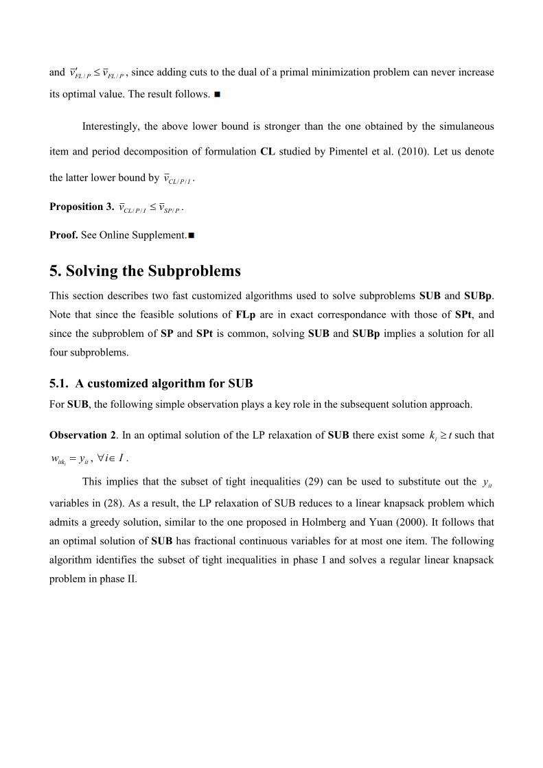
For SUB, the following simple observation plays a key role in the subsequent solution approach.
Observation 2. In an optimal solution of the LP relaxation of SUB there exist some tki such that
ititk ywi , Ii .
This implies that the subset of tight inequalities (29) can be used to substitute out the ity
variables in (28). As a result, the LP relaxation of SUB reduces to a linear knapsack problem which
admits a greedy solution, similar to the one proposed in Holmberg and Yuan (2000). It follows that
an optimal solution of SUB has fractional continuous variables for at most one item. The following
algorithm identifies the subset of tight inequalities in phase I and solves a regular linear knapsack
problem in phase II.
ALGORITHM SUB (for period t)
Phase I
IitkTkdvt
csr
ikit
ikitkitk
,|,
. iK Ø, ||,..., TtP , FalseBesti Ii,
For each Ii :
While FalseBesti :
itiitkKPkit rkrri
arg;min \ // min ratio calculation
iii kKK ; Replace
i
i
Kk ikitit
Kk ikitkit
itdvtst
csscr
// Update set and ratio of
If itkKPkit rri\min or PKi then // periods merged so far
TrueBesti // If ratio of merged periods is not min, exit
If itkKPkit rri\min then iii kKK \ // Retain best set of merged periods
i
i
Kk ikititit
Kk ikitkitit
dvtstvtm
csscvcm // Define cost and weight of merged periods
End If
End While
End For
Phase II
Solve a linear knapsack with weights IiKkdvtvtm iikitit ,; and costs
IiKkcscsm iitkit ,; .
Let IiKkwwm iitkit ,; denote the optimal solution.
Set IiKkwmy iitit ,, .
Return tkIiwy itkit ,, .
Phase I identifies which of the variable upper bound constraints (29) are satisfied as
equalities. Then, the value of the setup variable is set equal to the value of the production variable
with the most attractive cost-to-weight ratio. If the new ratio is still the most attractive after the
substitution, Phase I terminates for that item. If it is not, another constraint (29) is tight for the same
item, and the corresponding substitution is made. Phase II solves a linear knapsack problem where
all itkw with iKk are equated with ity and substituted out. Note that adjusting the algorithm to
tackle items with zero setup time or cost is straightforward. Due to observation 2, algorithm SUB
produces an optimal solution of the SUB linear relaxation.
After solving the relaxation, a depth-first branch-and-bound algorithm is implemented.
Branching is needed only when some itwm was the last variable to enter the knapsack at fractional
level, and therefore 1ity . Thus, at most one setup variable is fractional. In addition, branching does
not change the problem structure because it either fixes itkw to zero when 0ity or reduces the
problem capacity by itst and fixes itsc in the objective, when 1ity . For this reason, algorithm SUB
can be called at each node of the branch-and-bound tree, with different input data. Computational
experiments confirm the superiority of this approach compared to simplex-based branch-and-bound.
5.2. A customized algorithm for SUBp
The addition of the precedence constraints changes the structure of subproblem SUB and the
previous algorithm cannot be employed. However, we can take advantage of the fact that each
solution of SUBp corresponds to a solution of the SP/P subproblem (9)-(12), whose relaxation is a
linear multiple choice knapsack problem (Jans and Degraeve 2004) that can be solved efficiently
using the sorting algorithm of Sinha and Zoltners (1979). Therefore, we solve the subproblem (9)-
(12) and then map back the solution to SUBp. Sinha and Zoltners call a variable dominated if there
exists another variable, or a convex combination of other variables, that has a smaller or equal weight
and a smaller or equal cost. Dominated variables can be eliminated, and the remaining variables
enter the knapsack under a greedy sorting criterion. It is important to observe that the non-dominated
variables form the convex envelope of all variables when graphed in the (weight, cost) space. We use
the procedure of Sinha and Zoltners to solve the linear relaxations of (9)-(12) and to develop a
customized depth-first branch-and-bound algorithm. The multiple choice knapsack structure is
preserved in every node of the branch-and-bound tree, but the cost coefficients of some variables
change as the setup costs change with branching. This means that the convex envelopes do not need
to be fully reconstructed in each node, since only a few variables change positions. We use a variant
of the algorithm suggested by Graham (1972) to construct and update the convex hulls. Graham’s
algorithm determines the convex envelope of a set of n points in O(nlogn) time. This implies that
solving the linear relaxation of (9)-(12) in every node takes O(nlogn) time, and therefore this method
has better complexity compared to using the simplex algorithm.
6. Solving the RM Problem: a new Hybrid Algorithm
Huisman et al. (2005) discuss how exploiting the relationship between Dantzig-Wolfe
decomposition and Lagrange relaxation can lead to the development of improved algorithms that
combine the strengths of both methods. They explore two different ways to combine column
generation and Lagrange relaxation. First, Lagrange relaxation can be used to solve the RM, by
dualizing the linking constraints, and the resulting near-optimal dual values can be used to price out
the subproblems. Second, Lagrange relaxation on the original formulation can be employed within
column generation, exploiting the fact that both methods solve the same subproblem. Specifically,
the RM programs are solved with simplex, and next the RM dual prices are used as a starting point
for a number of Lagrange relaxation iterations, during which several negative reduced cost columns
can be found and added to the RM at once. We propose a new method, which is a combination of
the two previously discussed methods. Specifically, it uses Lagrange relaxation of the RM to solve
this RM program, and it also uses Lagrange relaxation on the original formulation to generate new
columns. Figure 2 gives a schematic representation of the algorithm. Implementation details can be
found in the online supplement that accompanies this paper.
Figure 2: The main building blocks of the new hybrid algorithm
We initialize the column generation process using the heuristic of Trigeiro et al. (1989). This
is a fast heuristic that performs several rounds of smoothing and rounding operations. For the
instances that Trigeiro et al. (1989) generated, their heuristic can find high quality feasible solutions,
giving integrality gaps lower than 3% on most problems. This heuristic returns a feasible solution, a
lower bound and a set of lagrangian dual prices of the capacity constraints. Using the dual of the
relaxation of SP or FL, we can then calculate the starting dual prices it . Also, the feasible solution
F
itit xy ),( is split into per period columns of the SPt or FLp RM programs. To perform this
operation, it is necessary to transform the F
itit xy ),( solution to the space of the extended formulation
variables. This can be done by fixing the setup variables to their given values and solving the
corresponding formulation, which is a shortest path problem. Next, the Lagrange relaxation
subroutine uses the modified subgradient method of Crowder (1976) to update the dual prices it .
The modified subgradient method is a variant of the traditional subgradient method that incorporates

past history in each iteration by searching in a direction that is the weighted average of the current
vector of violations and the previous searched direction. Computational experiments in Barahona and
Anbil (2000) show that the convergence of this variant is a lot faster compared to the regular
subgradient method. For each updated set of dual prices it we check if the subproblem solutions
price out, using the last obtained dual prices of the convexity constraints, t . The columns that price
out are added to the RM. Existing columns with a high reduced cost are removed from the RM and
kept into a separate column pool. Then, the RM problem is solved using subgradient optimization by
relaxing the linking constraints (23) (Huisman et al. 2005). Specifically, the dualization of
constraints (23) decomposes the RM into separate subproblems per period, each of which is of the
form
tt Sq
ittqtq
Ii
it
Ii
ititit
Ii Sq
tqittq spspcuct 0,0;1|)()(min . These problems
are trivially solved by setting the tq variable that has the minimum cost coefficient to one, and all
other variables to zero. The scheme iterates until no column prices out. We then invoke the volume
algorithm to obtain an approximate primal solution. In this way, we are able to make better informed
branching decisions in the subsequent branch-and-price phase. An alternative implementation would
be to use the intermediate dual prices of the subgradient optimization of the RM problem to price out
new columns. Our experiments with this strategy revealed that the generated columns are not of good
quality, because the intermediate dual prices of the RM problem price out many columns that do not
price out with its terminal dual prices. Instead, using the near optimal dual prices to warm-start the
lagrange relaxation produced better results and resulted in fewer iterations of the hybrid scheme.
Contrary to existing hybrid algorithms (Barahona and Jensen, 1998, Degraeve and Peeters
2003, Degraeve and Jans 2007), this scheme relies exclusively on Lagrange relaxation. It has the
benefits that it (a) avoids the degeneracy issues of the simplex method and therefore exibits faster
convergence and (b) returns good quality dual prices that help the column generation convergence.
Note that the intermediate value of the RM programs, Mv , is not necessarily a valid upper bound of
the column generation lower bound, as it is calculated using lagrange relaxation. It is a valid lower
bound (Huisman et al. 2005) when no column prices out, and therefore the scheme returns the best
bound that is obtained by the RM and by Lagrange relaxation.
7. A Branch-and-Price Heuristic
We have combined the hybrid column generation algorithm with heuristic techniques, and integrated
them in an enumeration scheme, using formulation FLp. The goal is to find good feasible solutions
fast by exploiting the structure of the network formulation and its subproblem. The next section
describes the heuristics employed in each node of the tree.
7.1 Node Heuristics
We employ a successive rounding heuristic that uses a smoothing subroutine, which in turn employs
some operations of the heuristic of Trigeiro et al. (1989). The successive rounding heuristic gets as
input the setup variables produced by the volume algorithm, determines a threshold level and fixes
the setup variables below and above that threshold to 0 and 1, respectively. The process iterates for
increasing threshold values. Typically, the objective function values of the feasible solutions
obtained in this way follow a U-shaped fashion (Degraeve and Jans 2007). Therefore, when the
solution quality starts to degrade the heuristic terminates. Starting from this solution, the smoothing
heuristic that searches for an improved feasible solution is applied. The smoothing part starts from
the last period and tries to push production backwards, such that the Lagrange costs are minimized.
This is done iteratively until the first period, and if any capacity constraints are violated it performs a
similar forward operation to recover feasibility. Thus, the rounding/smoothing heuristic scheme
searches the feasible space by modifying incrementally the proposed setup schedules and production
plans and can be classified as an exploitation heuristic.
7.2 Node Lower Bounds
At each node we solve the RM problem using subgradient optimization, without generating any
columns. If its objective value is lower than the incumbent value, we recover an approximate primal
solution using the volume algorithm and use that solution to branch. Else, if the RM objective value
is higher than the incumbent value, the hybrid algorithm is invoked to generate columns. During the
hybrid algorithm iterations, a non-decreasing node lower bound is recorded. If that lower bound
comes to exceed the incumbent value, the node is pruned. When the hybrid algorithm terminates and
the lower bound is below the incumbent value, the volume algorithm is invoked to recover an
approximate primal solution of the RM, which is then used for branching. When the volume
algorithm returns all-integer setup variables, we fix these variables and solve the resulting LP
problem using formulation CL, which is a generalized network flow problem for fixed setups
(Degraeve and Jans 2007). More details about this procedure can be found in the online supplement
of this paper.
7.3 Tree Exploration Strategies
Algorithm HBP summarizes the main building blocks of the heuristic Branch and Price algorithm.
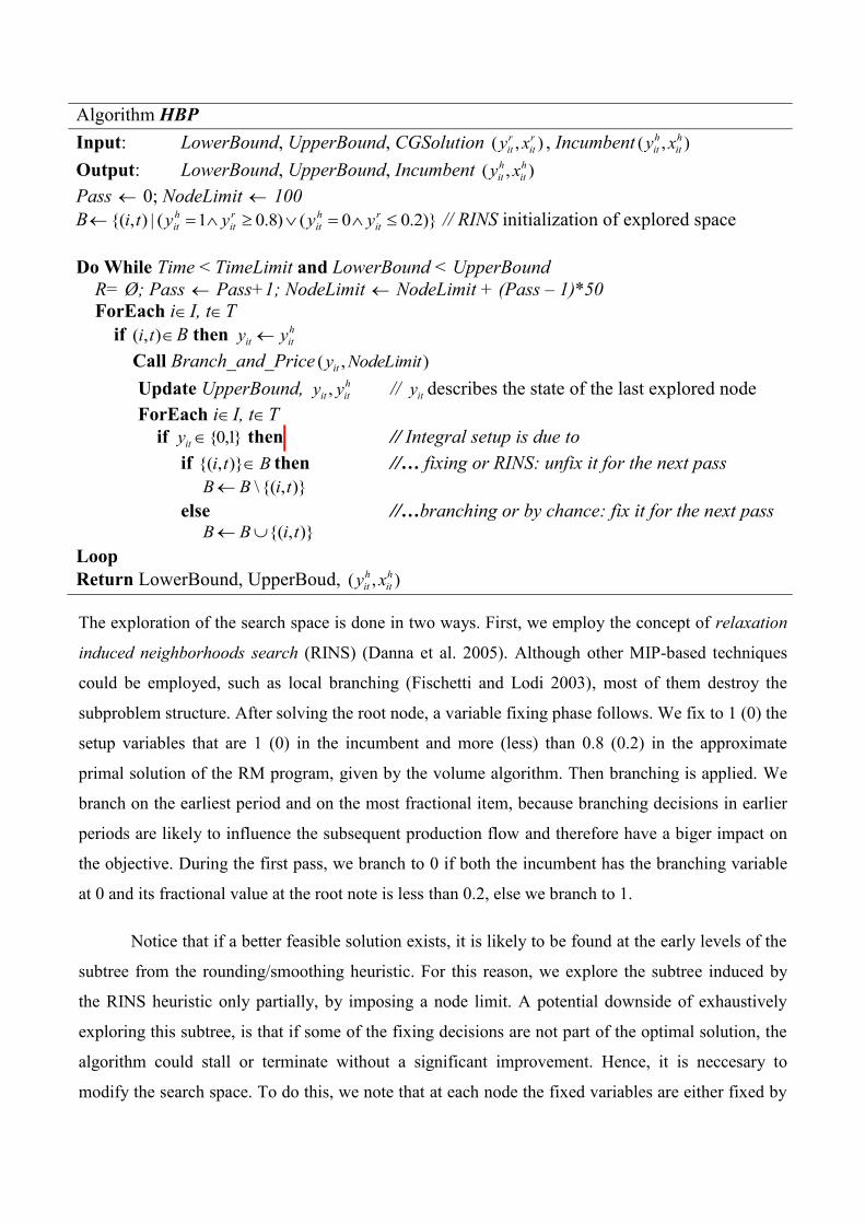
Algorithm HBP
Input: LowerBound, UpperBound, CGSolution ),( r
it
r
it xy , Incumbent ),( h
it
h
it xy
Output: LowerBound, UpperBound, Incumbent ),( h
it
h
it xy
Pass 0; NodeLimit 100
B )}2.00()8.01(|),{( r
it
h
it
r
it
h
it yyyyti // RINS initialization of explored space
Do While Time < TimeLimit and LowerBound < UpperBound
R= Ø; Pass Pass+1; NodeLimit NodeLimit + (Pass – 1)*50
ForEach iI, tT
if ),( ti B then h
itit yy
Call Branch_and_Price ),( NodeLimityit
Update UpperBound, h
itit yy , // ity describes the state of the last explored node
ForEach iI, tT
if }1,0{ity then // Integral setup is due to
if Bti )},{( then //… fixing or RINS: unfix it for the next pass
)},{(\ tiBB
else //…branching or by chance: fix it for the next pass )},{( tiBB
Loop
Return LowerBound, UpperBoud, ),( h
it
h
it xy
The exploration of the search space is done in two ways. First, we employ the concept of relaxation
induced neighborhoods search (RINS) (Danna et al. 2005). Although other MIP-based techniques
could be employed, such as local branching (Fischetti and Lodi 2003), most of them destroy the
subproblem structure. After solving the root node, a variable fixing phase follows. We fix to 1 (0) the
setup variables that are 1 (0) in the incumbent and more (less) than 0.8 (0.2) in the approximate
primal solution of the RM program, given by the volume algorithm. Then branching is applied. We
branch on the earliest period and on the most fractional item, because branching decisions in earlier
periods are likely to influence the subsequent production flow and therefore have a biger impact on
the objective. During the first pass, we branch to 0 if both the incumbent has the branching variable
at 0 and its fractional value at the root note is less than 0.2, else we branch to 1.
Notice that if a better feasible solution exists, it is likely to be found at the early levels of the
subtree from the rounding/smoothing heuristic. For this reason, we explore the subtree induced by
the RINS heuristic only partially, by imposing a node limit. A potential downside of exhaustively
exploring this subtree, is that if some of the fixing decisions are not part of the optimal solution, the
algorithm could stall or terminate without a significant improvement. Hence, it is neccesary to
modify the search space. To do this, we note that at each node the fixed variables are either fixed by
the RINS fixing decisions, or by branching. To explore a different but promising part of the setup
variable space, we free the variables fixed by RINS and fix the variables that were fixed by
branching to the values of the incumbent solution. The variables that were free at the last explored
node of the previous pass also remain free in the new pass. In a sense, this scheme tries to replace
dive decisions with branching decisions, while remaining close to the neighborhood of the
incumbent. The same idea is applied iteratively: a number of nodes in each subtree is explored, the
variables fixed early up in the free become free and the variables fixed from Branch and Price are
fixed again to the value of the incumbent.
8. Computational Results
Computational experiments were performed on a 2.0 GHz / 2 GB machine. The CPU times listed in
all tables for our heuristic refer to the time that the incumbent was found. To better undestand the
contribution of the developed methodology to the current literature, we have compared our algorithm
with other approaches found in the literature. The datasets that appear in the lot sizing literature and
are used in this paper have time-invariant setup, holding and production costs, and therefore are
special cases of our formulations, that also capture time-varying costs. We find that our approach
computes strong lower bounds fast and delivers high quality feasible solutions, when compared with
other approaches. However, since other approaches have different implementations and run under
different machines, the results have to be taken with a grain of salt. It is inevitable some authors use
more or less powerful machines, and different versions of commercial software, such as CPLEX,
which could introduce some bias in the result. We note however, that the quality of the lower bound
we obtain is implementation independent and that our algorithm uses a commercial package to solve
linear programs only. To the best of our knowledge, all lower bounds obtained by the methods
considered in this section are also independent of the solver used. An example of a solver-dependent
lower bound is the one of Van Vyve and Wolsey (2006). The authors let the XPRESS-MP solver
generate additional cuts by adding redundant inequalities in their formulation, and therefore the
lower bound quality depends on the underlying technology being used. We believe that the obtained
results offer some insight on how strong the obtained lower bound is, and how efficiently it can be
utilized in the search of feasible solutions. Detailed results of all experiments can be found in the
online supplement of this paper.
8.1 Solving the root node
8.1.1 Benchmarking of formulations and solution methods
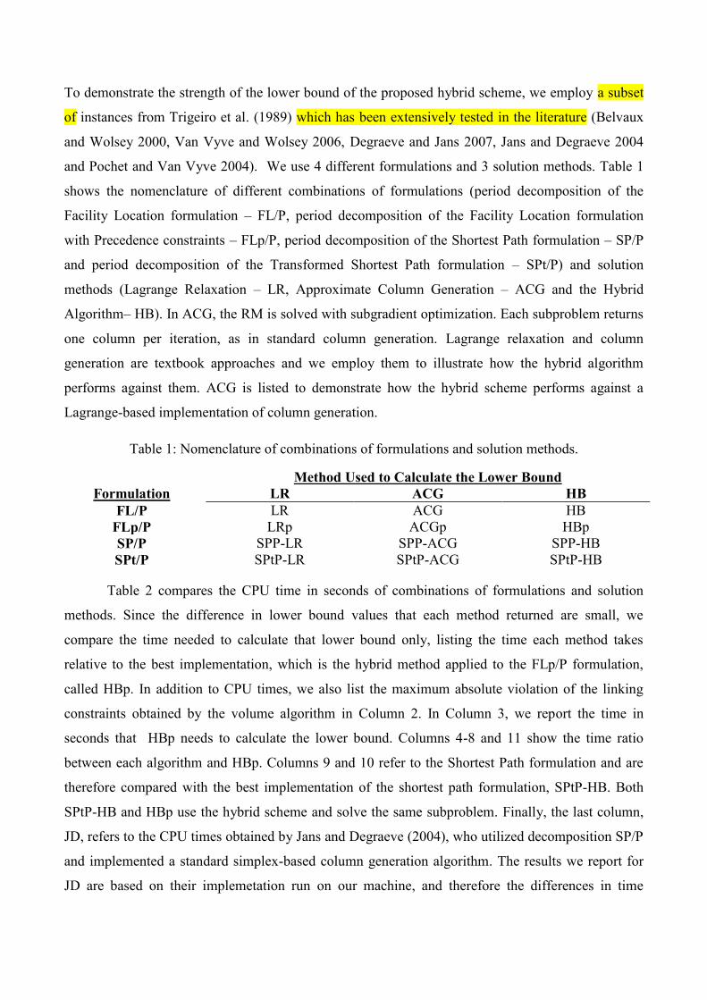
To demonstrate the strength of the lower bound of the proposed hybrid scheme, we employ a subset
of instances from Trigeiro et al. (1989) which has been extensively tested in the literature (Belvaux
and Wolsey 2000, Van Vyve and Wolsey 2006, Degraeve and Jans 2007, Jans and Degraeve 2004
and Pochet and Van Vyve 2004). We use 4 different formulations and 3 solution methods. Table 1
shows the nomenclature of different combinations of formulations (period decomposition of the
Facility Location formulation – FL/P, period decomposition of the Facility Location formulation
with Precedence constraints – FLp/P, period decomposition of the Shortest Path formulation – SP/P
and period decomposition of the Transformed Shortest Path formulation – SPt/P) and solution
methods (Lagrange Relaxation – LR, Approximate Column Generation – ACG and the Hybrid
Algorithm– HB). In ACG, the RM is solved with subgradient optimization. Each subproblem returns
one column per iteration, as in standard column generation. Lagrange relaxation and column
generation are textbook approaches and we employ them to illustrate how the hybrid algorithm
performs against them. ACG is listed to demonstrate how the hybrid scheme performs against a
Lagrange-based implementation of column generation.
Table 1: Nomenclature of combinations of formulations and solution methods.
Method Used to Calculate the Lower Bound
Formulation LR ACG HB
FL/P LR ACG HB
FLp/P LRp ACGp HBp
SP/P SPP-LR SPP-ACG SPP-HB
SPt/P SPtP-LR SPtP-ACG SPtP-HB
Table 2 compares the CPU time in seconds of combinations of formulations and solution
methods. Since the difference in lower bound values that each method returned are small, we
compare the time needed to calculate that lower bound only, listing the time each method takes
relative to the best implementation, which is the hybrid method applied to the FLp/P formulation,
called HBp. In addition to CPU times, we also list the maximum absolute violation of the linking
constraints obtained by the volume algorithm in Column 2. In Column 3, we report the time in
seconds that HBp needs to calculate the lower bound. Columns 4-8 and 11 show the time ratio
between each algorithm and HBp. Columns 9 and 10 refer to the Shortest Path formulation and are
therefore compared with the best implementation of the shortest path formulation, SPtP-HB. Both
SPtP-HB and HBp use the hybrid scheme and solve the same subproblem. Finally, the last column,
JD, refers to the CPU times obtained by Jans and Degraeve (2004), who utilized decomposition SP/P
and implemented a standard simplex-based column generation algorithm. The results we report for
JD are based on their implemetation run on our machine, and therefore the differences in time
performance can be attributed to the relative efficacy of our new hybrid methodology. Note that for
G57 and G72, we compare to their Lagrange relaxation times (2000 iterations), as they were not able
to solve these instances with simplex-based column generation. For the sake of brevity, we do not
present full results for formulations SP/P and SPt/P, since their behavior is very similary to that of
FL/P and FLp/P respectively. However, we do show that the hybrid solution method HB is superior
to Lagrange Relaxation LR and that LR applied to the transformed formulation SPt/P is much faster
than when applied to the standard formulation SP/P.
Table 2: Computational performance of different algorithms for obtaining the lower bound
Dataset HBp Max
Violation
Time
HBp (s)
HB /
HBp
LR /
HBp
LRp /
HBp
ACG /
HBp
ACGp/
HBp
SPP-LR/
SPtP-HB
SPtP-LR/
SPtP-HB
JD (SP/P)/
HBp
G30 (6-15) 0.032 0.18 2.0 8.9 3.1 9.6 9.3 4.89 1.52 2.4
G30b (6-15) 0.049 0.2 1.3 11.9 3.8 7.1 6.7 11.67 3.08 2.8
G53 (12-15) 0.016 1.6 0.9 4.6 1.2 3.5 3.5 6.45 2.90 3.1
G57 (24-15) 0.023 7.60 2.2 5.8 2.3 3.8 3.9 4.70 1.39 14.9*
G62 (6-30) 0.029 0.55 1.1 7.2 2.6 15.3 12.6 4.76 1.53 2.9
G69 (12-30) 0.025 2.43 2.2 9.6 2.4 12.4 14.5 7.04 1.77 22.2
G72 (24-30) 0.031 15.77 2.3 6.9 1.6 12.0 11.1 2.73 1.40 4.0*
Average 0.029 4.0 1.7 7.8 2.4 9.1 8.8 6.0 1.9 7.5
* Column generation did not terminate due to numerical issues, comparison with Lagrange relaxation
The comparison of the different approaches suggests some interesting conclusions. First, the
small violations in column 2 suggest that the approximate primal solution recovered by the volume
algorithm is very close to the exact primal solution. Second, The addition of the precedence
constraints to the facility location formulation (column 4), and the transformation of the shortest path
formulation (column 9 versus column 10) enhance the computational performance of LR and HB.
We see that on average HB needs 1.7 times the time of HBp to converge (column 4). Further, in
columns 5-8 it is evident that the effect of the precedence constraints is much stronger when using
LR instead of ACG. When comparing columns 5 and 6, we see that LRp is approximately 3 times
faster than LR, whereas columns 7 and 8 reveal that the performance of ACG and ACGp is
approximately the same. The precedence constraints influence the structure of the solutions returned
by the subproblems. These solutions are used by LR to update the dual prices in every iteration, and
therefore have a direct effect on the performance of the LR algorithm. ACG however, uses the
subproblem solutions as additional columns, and therefore they have an influence only if they are
active in an optimal solution of the restricted master problem. This might explain why the
precedence constraints lead to a big, medium and minimum improvement when applied to LR, HB
and ACG respectively. In addition, columns 9 and 10 reveal that the Lagrange relaxation of the

shortest path formulation is approximately 3 times slower, on average, compared to its transformed
version. Algorithms SPP-ACG, SPtP-ACG and SPP-HB showed similar behavior as ACG, ACGp
and HB respectively and are not reported. The hybrid scheme outperforms all approaches. On
average, HBp is five times faster than the other algorithms. Finally, it is interesting to note that for
JD, an implementation of simplex-based column generation, the CPU times are disproportionally
larger, indicating the poor performance of simplex-based column generation.
8.1.2 Comparison of lower and upper bounds with other approaches
On assessing the lower bound quality obtained by SP/P, Jans and Degraeve (2004) give evidence that
for the 7 instances of Table 2, this lower bound is stronger than the one obtained by Trigeiro et al.
(1989), Degraeve and Jans (2007), Belvaux and Wolsey (2000) and Miller et al. (2000a), while the
bound from Van Vyve and Wolsey (2006) seems to be stronger for most instances. Note however
that there is no theoretical ground to support arguments that one bound dominates another bound,
with the exception of the bound given by Trigeiro et al. (1989), which is not better than the bound of
Jans and Degraeve (2004). Therefore, the performance of each methodology is data dependent.
Intuitively, the period decomposition should perform well when the capacity constraints are tight,
because it takes advantage of the extreme points of the single-period polytopes, and when the
number of items is small, which is likely to make the subproblems easier.
In another experiment, we compared the performance of our algorithm to the results obtained
by Süral et al. (2009). They design a Lagrange-based heuristic for a reformulation of the capacitated
problem with setup times but without setup costs. The demand constraint is relaxed. They modify the
data from Trigeiro et al. (1989) as follows. First, they set all setup costs to zero. Second, they
increase zero demands to 2 units. Third, they construct new instances by reducing the number of
periods of some existing ones. Finally, they construct instances with unit inventory costs for all
items, called homogeneous (denoted “hom”). Instances with the original inventory cost are called
heterogeneous (denoted “het”). In total, 100 instances are generated. Since their approach usually
terminates in a few seconds, we have chosen to compare it with our hybrid procedure only.
Specifically, we use the hybrid process to obtain a lower bound, recover an approximate primal
solution with the volume algorithm, fix the setup variables to 0 or 1 (as described in the diving
heuristic) and call the successive rounding/smoothing heuristic once. In particular, no branching is
performed, and the algorithm is actually the procedure that is performed at the root node of the
branch-and-price tree. We call this procedure the restricted hybrid heuristic (RHB). Table 3 displays
the average duality gaps and the average CPU time for the best heuristic approach of Süral et al.
(SDW) and our restricted hybrid heuristic (RHB). SDW was run on an Intel Pentium 4 machine, and
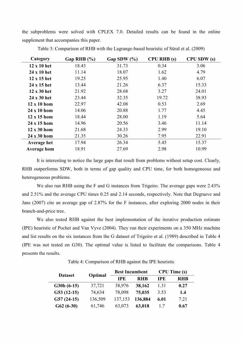
the subproblems were solved with CPLEX 7.0. Detailed results can be found in the online
supplement that accompanies this paper.
Table 3: Comparison of RHB with the Lagrange-based heuristic of Süral et al. (2009)
Category Gap RHB (%) Gap SDW (%) CPU RHB (s) CPU SDW (s)
12 x 10 het 18.43 31.73 0.34 3.06
24 x 10 het 11.14 18.07 1.62 4.79
12 x 15 het 19.25 25.95 1.40 6.07
24 x 15 het 13.44 21.26 6.37 15.33
12 x 30 het 21.92 28.68 3.27 24.01
24 x 30 het 23.44 32.35 19.72 38.93
12 x 10 hom 22.97 42.08 0.53 2.69
24 x 10 hom 14.06 20.88 1.77 4.45
12 x 15 hom 18.44 28.00 1.19 5.64
24 x 15 hom 14.96 20.56 3.46 11.14
12 x 30 hom 21.68 24.33 2.99 19.10
24 x 30 hom 21.35 30.26 7.95 22.91
Average het 17.94 26.34 5.45 15.37
Average hom 18.91 27.69 2.98 10.99
It is interesting to notice the large gaps that result from problems without setup cost. Clearly,
RHB outperforms SDW, both in terms of gap quality and CPU time, for both homogeneous and
heterogeneous problems.
We also run RHB using the F and G instances from Trigeiro. The average gaps were 2.43%
and 2.51% and the average CPU times 0.25 and 2.14 seconds, respectively. Note that Degraeve and
Jans (2007) cite an average gap of 2.87% for the F instances, after exploring 2000 nodes in their
branch-and-price tree.
We also tested RHB against the best implementation of the iterative production estimate
(IPE) heuristic of Pochet and Van Vyve (2004). They run their experiments on a 350 MHz machine
and list results on the six instances from the G dataset of Trigeiro et al. (1989) described in Table 4
(IPE was not tested on G30). The optimal value is listed to facilitate the comparisons. Table 4
presents the results.
Table 4: Comparison of RHB against the IPE heuristic
Dataset Optimal Best Incumbent CPU Time (s)
IPE RHB IPE RHB
G30b (6-15) 37,721 38,976 38,162 1.31 0.27
G53 (12-15) 74,634 78,098 75,035 3.53 1.4
G57 (24-15) 136,509 137,153 136,884 6.01 7.21
G62 (6-30) 61,746 63,073 63,018 1.7 0.67
G69 (12-30) 130,596 131,988 131,668 6.03 3.38
G72 (24-30) 287,929 290,006 288,313 21.15 15.5
Although a comparison of CPU Times is hard since different machines were used, it is clear
that the quality of feasible solutions is much better for RHB. Note that the above IPE results are the
best that Pochet and Van Vyve cite, based on the BC-PROD cut generator. Also, despite that RHB
seems to find a better feasible solution than IPE, more space for improvement exists, as shown by the
optimal solutions. The branch-and-price heuristic performs RHB at the root node and tries to
approach the optimal solution. Its computational peformance is described in section 8.2.
8.2 Comparison of heuristic branch-and-price with other approaches
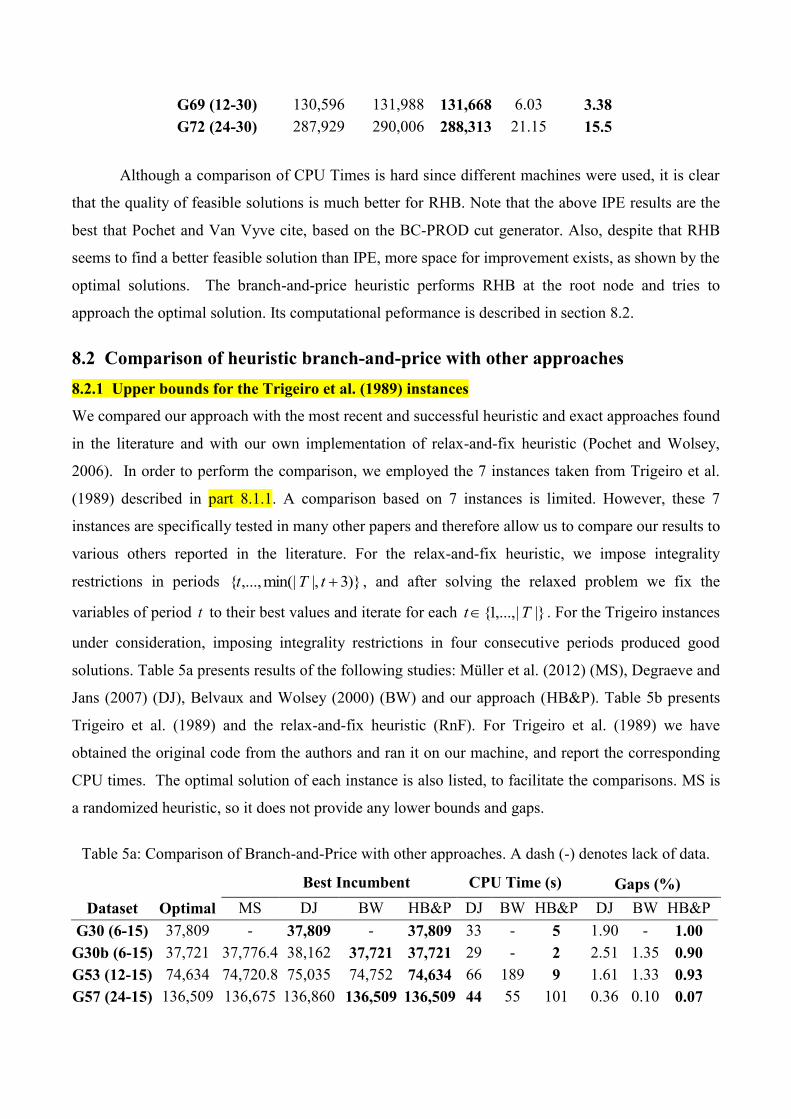
8.2.1 Upper bounds for the Trigeiro et al. (1989) instances
We compared our approach with the most recent and successful heuristic and exact approaches found
in the literature and with our own implementation of relax-and-fix heuristic (Pochet and Wolsey,
2006). In order to perform the comparison, we employed the 7 instances taken from Trigeiro et al.
(1989) described in part 8.1.1. A comparison based on 7 instances is limited. However, these 7
instances are specifically tested in many other papers and therefore allow us to compare our results to
various others reported in the literature. For the relax-and-fix heuristic, we impose integrality
restrictions in periods )}3|,min(|,...,{ tTt , and after solving the relaxed problem we fix the
variables of period t to their best values and iterate for each |}|,...,1{ Tt . For the Trigeiro instances
under consideration, imposing integrality restrictions in four consecutive periods produced good
solutions. Table 5a presents results of the following studies: Müller et al. (2012) (MS), Degraeve and
Jans (2007) (DJ), Belvaux and Wolsey (2000) (BW) and our approach (HB&P). Table 5b presents
Trigeiro et al. (1989) and the relax-and-fix heuristic (RnF). For Trigeiro et al. (1989) we have
obtained the original code from the authors and ran it on our machine, and report the corresponding
CPU times. The optimal solution of each instance is also listed, to facilitate the comparisons. MS is
a randomized heuristic, so it does not provide any lower bounds and gaps.
Table 5a: Comparison of Branch-and-Price with other approaches. A dash (-) denotes lack of data.
Best Incumbent CPU Time (s) Gaps (%)
Dataset Optimal MS DJ BW HB&P DJ BW HB&P DJ BW HB&P
G30 (6-15) 37,809 - 37,809 - 37,809 33 - 5 1.90 - 1.00
G30b (6-15) 37,721 37,776.4 38,162 37,721 37,721 29 - 2 2.51 1.35 0.90
G53 (12-15) 74,634 74,720.8 75,035 74,752 74,634 66 189 9 1.61 1.33 0.93
G57 (24-15) 136,509 136,675 136,860 136,509 136,509 44 55 101 0.36 0.10 0.07
G62 (6-30) 61,746 61,792.2 62,644 61,746 61,746 359 55 140 2.79 1.24 0.88
G69 (12-30) 130,596 130,675 131,234 130,599 130,599 215 102 131 0.81 0.32 0.20
G72 (24-30) 287,929 287,966 288,383 287,950 288,016 306 298 46 0.22 0.07 0.07
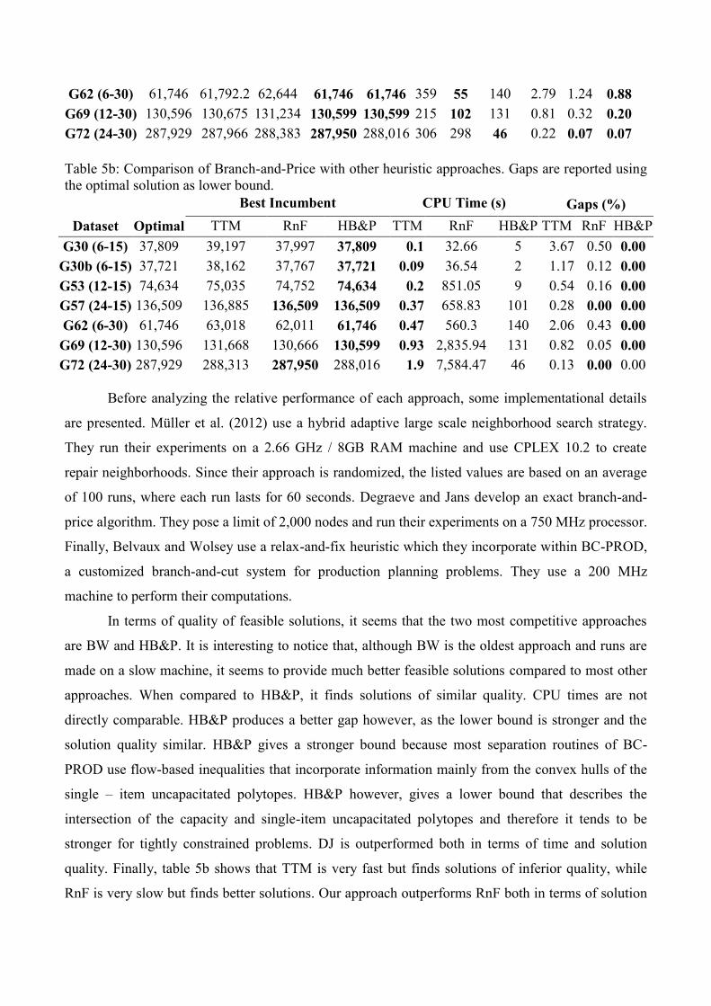
Table 5b: Comparison of Branch-and-Price with other heuristic approaches. Gaps are reported using
the optimal solution as lower bound.
Best Incumbent CPU Time (s) Gaps (%)
Dataset Optimal TTM RnF HB&P TTM RnF HB&P TTM RnF HB&P
G30 (6-15) 37,809 39,197 37,997 37,809 0.1 32.66 5 3.67 0.50 0.00
G30b (6-15) 37,721 38,162 37,767 37,721 0.09 36.54 2 1.17 0.12 0.00
G53 (12-15) 74,634 75,035 74,752 74,634 0.2 851.05 9 0.54 0.16 0.00
G57 (24-15) 136,509 136,885 136,509 136,509 0.37 658.83 101 0.28 0.00 0.00
G62 (6-30) 61,746 63,018 62,011 61,746 0.47 560.3 140 2.06 0.43 0.00
G69 (12-30) 130,596 131,668 130,666 130,599 0.93 2,835.94 131 0.82 0.05 0.00
G72 (24-30) 287,929 288,313 287,950 288,016 1.9 7,584.47 46 0.13 0.00 0.00
Before analyzing the relative performance of each approach, some implementational details
are presented. Müller et al. (2012) use a hybrid adaptive large scale neighborhood search strategy.
They run their experiments on a 2.66 GHz / 8GB RAM machine and use CPLEX 10.2 to create
repair neighborhoods. Since their approach is randomized, the listed values are based on an average
of 100 runs, where each run lasts for 60 seconds. Degraeve and Jans develop an exact branch-and-
price algorithm. They pose a limit of 2,000 nodes and run their experiments on a 750 MHz processor.
Finally, Belvaux and Wolsey use a relax-and-fix heuristic which they incorporate within BC-PROD,
a customized branch-and-cut system for production planning problems. They use a 200 MHz
machine to perform their computations.
In terms of quality of feasible solutions, it seems that the two most competitive approaches
are BW and HB&P. It is interesting to notice that, although BW is the oldest approach and runs are
made on a slow machine, it seems to provide much better feasible solutions compared to most other
approaches. When compared to HB&P, it finds solutions of similar quality. CPU times are not
directly comparable. HB&P produces a better gap however, as the lower bound is stronger and the
solution quality similar. HB&P gives a stronger bound because most separation routines of BC-
PROD use flow-based inequalities that incorporate information mainly from the convex hulls of the
single – item uncapacitated polytopes. HB&P however, gives a lower bound that describes the
intersection of the capacity and single-item uncapacitated polytopes and therefore it tends to be
stronger for tightly constrained problems. DJ is outperformed both in terms of time and solution
quality. Finally, table 5b shows that TTM is very fast but finds solutions of inferior quality, while
RnF is very slow but finds better solutions. Our approach outperforms RnF both in terms of solution
quality and CPU time. Since we use TTM to warm-start our algorithm, it is expected that we obtain
better solutions at a higher CPU time.
To the best of our knowledge, the best exact approach found in the literature for the above
instances from a lower bound perspective, is the approximate extended formulation of Van Vyve and
Wolsey (2006). Unfortunately, the authors do not cite the CPU time at which they obtain the lower
bound at the root node and a comparison with our approach is not possible. However it is expected
that a heuristic implementation of their approach would work better for problems with short time
horizon, whereas our approach is better for long horizon problems. For example, they solve G62 (6
items, 30 periods) to optimality after 220400 nodes and 1078 seconds on a 1.6GHz machine whereas
we need 4212 nodes and 140 seconds to find the optimal value (on a 2GHz machine).
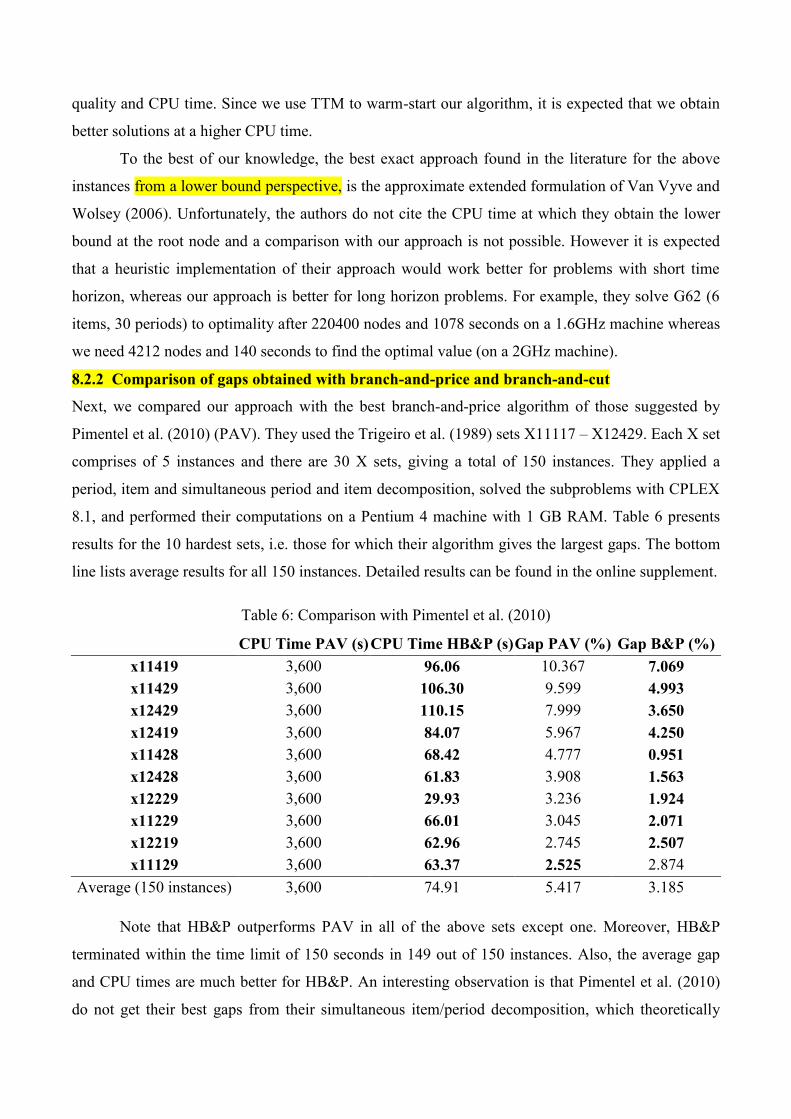
8.2.2 Comparison of gaps obtained with branch-and-price and branch-and-cut
Next, we compared our approach with the best branch-and-price algorithm of those suggested by
Pimentel et al. (2010) (PAV). They used the Trigeiro et al. (1989) sets X11117 – X12429. Each X set
comprises of 5 instances and there are 30 X sets, giving a total of 150 instances. They applied a
period, item and simultaneous period and item decomposition, solved the subproblems with CPLEX
8.1, and performed their computations on a Pentium 4 machine with 1 GB RAM. Table 6 presents
results for the 10 hardest sets, i.e. those for which their algorithm gives the largest gaps. The bottom
line lists average results for all 150 instances. Detailed results can be found in the online supplement.
Table 6: Comparison with Pimentel et al. (2010)
CPU Time PAV (s) CPU Time HB&P (s) Gap PAV (%) Gap B&P (%)
x11419 3,600 96.06 10.367 7.069
x11429 3,600 106.30 9.599 4.993
x12429 3,600 110.15 7.999 3.650
x12419 3,600 84.07 5.967 4.250
x11428 3,600 68.42 4.777 0.951
x12428 3,600 61.83 3.908 1.563
x12229 3,600 29.93 3.236 1.924
x11229 3,600 66.01 3.045 2.071
x12219 3,600 62.96 2.745 2.507
x11129 3,600 63.37 2.525 2.874
Average (150 instances) 3,600 74.91 5.417 3.185
Note that HB&P outperforms PAV in all of the above sets except one. Moreover, HB&P
terminated within the time limit of 150 seconds in 149 out of 150 instances. Also, the average gap
and CPU times are much better for HB&P. An interesting observation is that Pimentel et al. (2010)
do not get their best gaps from their simultaneous item/period decomposition, which theoretically
gives a stronger bound compared to both their item and period decompositions, but from the item
decomposition. This is because the RM problems of the simultaneous item/period decomposition are
very degenerate and time consuming. Therefore, they may not be able to obtain good feasible
solutions and improve their gap within their time limit.
In a final round of trials, we tested our algorithm on some new hard datasets against the
CPLEX v12.2 solver (CPX), using the regular formulation CL. The purpose of this comparison is to
give evidence on the relative strengths and weaknesses of a decomposition approach against a
modern off-the-self branch-and-cut software. To this end, we constructed new harder instances by
modifying the Trigeiro dataset. Specifically, we replicated the demand patterns to 60 periods, and
reduced the capacity to 95% of its original value. We focused on instances with 6 and 12 items
because the integrality gap of the extended formulations improves as the number of items increases,
therefore problems with fewer items are more challenging to solve. Finally, we excluded instances
that were infeasible without initial inventory because their gap was sensitive to the initial inventory
cost.
The process described above led to the creation of 30 new 60-period instances, 21 of which
have 6 items and 9 with 12 items. Table 7 shows the computational results. Both algorithms used 100
seconds of CPU time. This time limit is deemed appropriate for our approach, which can be used (i)
in a practical production environment, for fast generation of good quality production plans, or (ii) as
a warm-start method of an exact approach, such as branch-and-cut or branch-and-price.
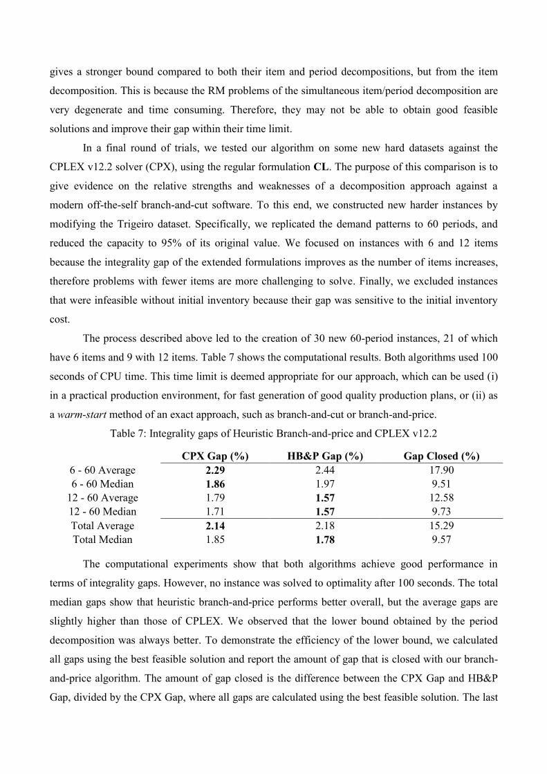
Table 7: Integrality gaps of Heuristic Branch-and-price and CPLEX v12.2
CPX Gap (%) HB&P Gap (%) Gap Closed (%)
6 - 60 Average 2.29 2.44 17.90
6 - 60 Median 1.86 1.97 9.51
12 - 60 Average 1.79 1.57 12.58
12 - 60 Median 1.71 1.57 9.73
Total Average 2.14 2.18 15.29
Total Median 1.85 1.78 9.57
The computational experiments show that both algorithms achieve good performance in
terms of integrality gaps. However, no instance was solved to optimality after 100 seconds. The total
median gaps show that heuristic branch-and-price performs better overall, but the average gaps are
slightly higher than those of CPLEX. We observed that the lower bound obtained by the period
decomposition was always better. To demonstrate the efficiency of the lower bound, we calculated
all gaps using the best feasible solution and report the amount of gap that is closed with our branch-
and-price algorithm. The amount of gap closed is the difference between the CPX Gap and HB&P
Gap, divided by the CPX Gap, where all gaps are calculated using the best feasible solution. The last
column indicates the superiority of the lower bound obtained by theperiod decomposition, as the
average gap improvement is about 15%. The lower bound obtained by CPLEX is weak, even after
exploring a large part of the branch-and-bound tree. Specifically, CPLEX explores more than 28,000
nodes on average, whereas we explore an average of 644 nodes with our approach. The fact that
CPLEX explores such a large part of the tree allows it to find better feasible solutions in most
instances, so its integrality gaps are competitive to branch-and-price. In conclusion, the two
approaches give similar results in terms of gap quality, but our approach dominates CPLEX in lower
bounds, since it takes advantage of the special structure of the single period polytopes.
9. Conclusions and future research
We have presented period decompositions of the facility location and shortest path formulations of
the capacitated lot sizing problem with setup times. The subproblems polytopes do not have the
integrality property, and therefore an improved lower bound is obtained. Customized branch-and-
bound algorithms are developed to solve the single-period subproblems. In addition, a novel,
subgradient-based algorithm is developed, that combines column generation with Lagrange
relaxation, and uses the volume algorithm to recover an approximate primal solution of the RM
problem. The performance of the hybrid scheme is enhanced further with the proposition of a
transformed shortest path formulation and with the addition of a class of valid inequalities in the
subproblem. The resulting subproblem is still tractable with a fast customized branch-and-bound
algorithm. Finally, a branch-and-price based heuristic is designed, that integrates relaxation induced
neighborhoods, selective diving and successive rounding/smoothing within a novel strategy of node
exploration. Computational results show that the proposed approach outperforms or compares
favorably with the most recent and successful approaches found in the literature.
The period decomposition formulations that we employ can be readily applied to lot sizing
problems with richer structure, such as backlogging, overtime and startup times. The subproblem
algorithms can also be adapted in a straightforward manner so that they incorporate these features.
The application of period decompositions to multi-level problems is strainghforward, but solving
problems with multiple resources, such as those introduced by Stadtler (2003) is computationally
more challenging. Although the period by period decomposition structure is retained when the
demand constraints are dualized, the resulting subproblems may not preserve the structures we
studied in this paper and new algorithms that solve their LP relaxations need to be devised. In
particular, whenever an item needs a setup or production time with respect to more than one resource
per period, the per-period subproblem involves multiple capacity constraints, and its linear relaxation
is no longer a linear multiple choice knapsack problem. Given the strong lower bounds that we
obtained for the CLST, an application to the multi-level instances is a promising area for future
research, especially because the best known lower bounds of these instances can be improved
considerably.
With respect to the developed methodology, there are several directions that deserve further
research. The implementation of standard stabilization techniques (eg. du Merle et al. 1999) to
extended formulations may make them more tractable computationally. Also, it could lead to the
development of an exact approach, for which an exact representation of the primal solution of the
RM is needed. On a different line, the integration of approximate schemes such as the volume
algorithm could lead to enhanced MIP-based heuristics that can tackle very large instances
efficiently and give a good dual bound, used to assess their performance. Finally, the period
decomposition could lead to the development of successful approximation algorithms. Recently,
Levi et al. (2008) used the simple plant location formulation with added flow cover inequalities to
derive the first 2-approximation algorithm for a variant of CLST without setup times. It would be
interesting to explore whether a column generation-based relaxation would lead to similar
approximation schemes for CLST.
Appendix
Proof of Theorem 1.
Theorem 1 states that DD ' where
)6(:,,
)5(,},min{
';
)4(,,
)3(,
)2(|}{|\,
)1(||:,,1
1
1
11
1,
AtkTktIicvv
ATtIicvciv
vD
ATtIicvv
AIiciv
ATTtIicivv
ATktTktIicvvv
vD
itk
k
tl
il
tiit
t
l
il
it
itmit
imi
ititi
itkkiit
it
Note that n
i
iDD1
and n
i
iDD1
''
and Ø1
'
1
n
i
i
n
i
i DD , and therefore each polyhedron is
separable per item. Also, without loss of generality we can restrict our attention to the positive
orthant of both dual spaces because (7) can be written as inequality ( ) and also (8) can be written as
inequality ( ). We will first show that DD ' . For this, consider a point 'Dvit . Note that (A5)
and (A6) imply (A3) and (A4). Supposing that (A6) holds, we show that (A1) holds as well. We
write (A6) as itkititk
U
k
tl
ilit cvUvcvvv 1
. Observe that if itkkiit cvvv 1, , then
011, ikititkkiit vUUvcvvv , which cannot hold because itv in both spaces.
Therefore, (A6) implies (A1). Using the same argument, (A5) implies (A2). This means that
DvDv itit ' for an arbitrary point 'Dvit , and thus DD ' .
We show that the inclusion may be strict via an example. Consider the following single-item 2-
period uncapacitated system with no initial inventory and its transformed version:
0,,,
][0
][1..)(
min
221211
22211
11211
222212121111
zzz
vzz
vzztsP
zczczc
0,,,
][1
][1..)'(
min
221211
22212
11211
222212121111
zzz
vzz
vzztsP
zczczc
The corresponding dual formulations are:
0,
..)(
max
21
222
121
1121
1
vv
cv
cv
cvvtsD
v
0,
..)'(
max
21
222
1221
111
21
vv
cv
cvv
cvtsD
vv
The point ),(),( 1121 cvv is feasible for )(D and infeasible for )'(D for a small 0 therefore
DD ' , and the proof is complete.
References
Alfieri, A., P. Brandimarte, S. D’Orazio 2002. LP-based heuristics for the capacitated lot-sizing
problem: the interaction of model formulation and solution algorithm. International Journal of
Production Research 40 441-458.
Barahona, F., D. Jensen. 1998. Plant location with minimum inventory. Mathematical
Programming 83 101-111.
Barahona, F., R. Anbil. 2000. The volume algorithm: producing primal solutions with a subgradient
method. Mathematical Programming 87 385-399.
Barany, I., T. Van Roy, L. Wolsey. 1984. Strong formulations for multi-item capacitated lot-sizing.
Management Science 30 1255-1261.
Ben Amor, H., J. Desrosiers, J.M. Valèrio de Carvalho. 2007. Dual-optimal inequalities for
stabilized column generation. Operations Research 54 454-463.
Belvaux, G., L. Wolsey. 2000. Bc-prod: A specialized branch-and-cut system for lot-sizing
problems. Management Science 46 724-738.
Buschkühl, L. F. Sahling, S. Helber, H. Tempelmeier. 2010. Dynamic capacitated lot-sizing
problems: a classification and review of solution approaches. OR Spectrum 32 231-261.
Caserta, M., E.Q. Rico. 2009. A cross-entropy lagrangian hybrid algorithm for the multi-item
capacitated lot-sizing problem with setup times. Computers and Operations Research 36 530-
548.
Crowder, H. 1976. Computational improvements for subgradient optimization. Symposium
Mathematica XIX 357 – 372
Danna, E., E. Rothberg, C. Le Pape. 2005. Exploring relaxation induced neighborhoods to improve
MIP solutions. Mathematical Programming Series A 102 71-90.
Degraeve, Z., M. Peeters. 2003. Optimal integer solutions to industrial cutting-stock problems: Part
2, Benchmark results. INFORMS Journal on Computing 15 58-81.
Degraeve, Z., R. Jans. 2007. A new Danzig-Wolfe reformulation and branch-and-price algorithm
for the capacitated lot-sizing problem with setup times. Operations Research 55 909-920.
Denizel, M., F. T. Altekin, H. Süral, H. Stadtler 2008. Equivalence of the LP relaxation of two
strong formulations for the capacitated lot-sizing problem with setup times. OR spectrum 30
773-785.
Denizel, M., H. Süral 2006. On alternative mixed integer programming formulation and LB-based
heuristics for lot-sizing with setup times. Journal of the Operational Research Society 57
389-399.
Du Merle, O., D. Villeneuve, J. Desrosiers, P. Hansen. 1999. Stabilized column generation.
Discrete Mathematics 194 229-237.
Eppen, G.D., R.K. Martin. 1987. Solving multi-item capacitated lot-sizing problems using variable
redefinition. Operations Research 35 832-848.
Fiorotto, D. J. , S. A. de Araujo. 2014. Reformulation and a Lagrangian heuristic for lot sizing
problem on parallel machines. Published online at Annal of Operations Research.
Fischetti, M., A. Lodi. 2003. Local branching. Mathematical Programming Ser. B 98 23-47.
Geoffrion, A. M. 1974. Lagrangean relaxation for integer programming. Mathematical Programming
Study 2 82-114.
Graham, R. L. 1972. An efficient algorithm for determining the convex hull of a finite planar set.
Information Processing Letters 1 132-133.
Helber, S., F. Sahling. 2010. A fix-and-optimize approach for the multi-level capacitated lot sizing
problem. International Journal of Production Economics 123 247-256.
Holmberg, K. , D. Yuan. 2000. A Lagrangean heuristic based branch-and-bound approach for the
capacitated network design problem. Operations Research 48 461-481.
Huisman, D., R. Jans, M. Peeters, A.P.M. Wagelmans. 2005. Combining column generation and
lagrangian relaxation. G. Desaulniers, J. Desrosiers, M. Solomon, eds. Column Generation.
Springer, New York, 247-270.
Jans, R., Z. Degraeve. 2004. Improved lower bounds for the capacitated lot-sizing problem with
setup times. Operations Research Letters 32 185-195.
Jans, R., Z. Degraeve. 2007. Meta-heuristics for dynamic lot-sizing: a review and comparison of
solution approaches. European Journal of Operational Research 177 1855-1875.
Krarup, J., I. Bilde. 1977. Plant location, set covering and economic lot size: an O(mn) algorithm for
structural problems. Numerische methoden bei optimierungsaufgaben, Band 3: optimierung bei
graphentheoretischen und ganzzahligen problemen, Vol. 36, Birkhauser Verlag, Basel and
Stuttgart, 1977.
Levi, R. A. Lodi, M. Sviridenko. 2008. Approximation algorithms for the capacitated multi-item lot-
sizing problems via flow-cover inequalities. Mathematics of Operations Research 33 461-474.
Lübbecke, M., J. Desrosiers. 2005. Selected topics in column generation. Operations Research 53
1007-1023.
Manne, A. S. 1958. Programming of economic lot sizes. Management Science 4(2) 115-135.
Miller, A.J., G.L. Nemhauser, M.W. Savelsberg. 2000a. Solving multi-item capacitated lot-sizing
problems with setup times by branch-and-cut. CORE Discussion paper 2000/39, UCL, Louvain-
la-Neuve, Belgium.
Miller, A.J., G.L. Nemhauser, M.W.P. Savelsbergh. 2000b. On the capacitated lot-sizing and
continuous 0—1 knapsack polyhedra. European Journal of Operational Research 125 (2) 298-
315.
Miller, A.J., G.L. Nemhauser, M.W.P. Savelsbergh. 2003. On the polyhedral structure of a multi-
item producting planning model with setup times. Mathematical Programming 94 (2-3) 375-405.
Müller, L.F., S. Spoorendonk, Pisinger, D. 2012. A hybrid adaptive large neighborhood search
heuristic for lot-sizing with setup times. European Journal of Operational Research 218 614-
623.
Pimentel, C.M.O., F.P. Alvelos, J.M. Valèrio de Carvalho. 2010. Comparing danzig-wolfe
decompositions and branch-and-price algorithms for the multi-item capacitated lot sizing
problem. Optimization Methods and Software. 25 299-319.
Pisinger, D. 1995. A minimal algorithm for the multiple-choice knapsack problem. European
Journal of Operational Research 83 394-410.
Pochet, Y., L. A. Wolsey. 2006. Production Planning by Mixed Integer Programming. Springer-
Verlag New York, Inc..
Pochet, Y., M. Van Vyve. 2004. A generic heuristic for production planning problems. INFORMS
Journal on Computing 16 316-327.
Sinha, P., A. Zoltners. 1979. The multiple-choice knapsack problem. Operations Research 27 (3)
503-515.
Stadtler, H. 2003. Multilevel lot sizing with setup times and multiple constrained resources:
Internally rolling schedules with lot-sizing windows. Operations Research 51 487-502.
Stadtler, H. 2007. Collaborative Planning – Concepts, Framework and Challenges. Operations
Research Proceedings, Springer Berlin Heidelberg.
Subramanian, S., H. Sherali. 2008. An effective deflective subgradient optimization scheme for
implementing column generation for large scale airline crew scheduling problems. INFORMS
Journal on Computing 20 565-578.
Süral, H., M. Denizel, L.N. Van Wassenhove. 2009. Lagrangean relaxation based heuristics for lot
sizing with setup times. European Journal of Operational Research 194 51-63.
Tempelmeier, H. 2011. A column generation heuristic for dynamic capacitated lot sizing with
random demand under a fill rate constraint. Omega 39 627-633.
Trigeiro, W., L.J. Thomas, J.O. McClain. 1989. Capacitated lot sizing with set-up times.
Management Science 35 353-366.
Van Vyve, M., L. Wolsey. 2006. Approximate extended formulations. Mathematical Programming
Series B 105 501-522.
Vanderbeck, F. 1998. Lot-sizing with start-up times. Management Science 44 1409-1425.
Vanderbeck, F., M. W. P. Savelsbergh. 2006. A generic view of Danzig-Wolfe decomposition in
mixed integer programming. Operations Research Letters 48 111-128.
Wolsey, L. 1989. Uncapacitated lot-sizing problems with start-up costs. Operations Research 37
741-747.

![The Fixed Charge Transportation Problem: A Strong ...Very few papers on Lagrangian decomposition and column generation: I [Pimentel et al.(2010)]: The multi-item capacitated lot sizing](https://img.pdfslide.us/doc/110x75/5f159c36c6ceac62f34c743f/the-fixed-charge-transportation-problem-a-strong-very-few-papers-on-lagrangian.jpg)