Duality Approaches to Economic Lot-Sizing Games

Xin Chen

Department of Industrial and Enterprise Systems Engineering

University of Illinois at Urbana-Champaign, Urbana, IL 61801.

Email: xinchen@illinois.edu. Phone: 217-244-8685

Jiawei Zhang

Stern School of Business, IOMS-Operations Management

New York University, New York, NY, 10012.

Email: jzhang@stern.nyu.edu. Phone: 212-998-0811

December 12, 2015

Abstract

Sharing common production, resources and services to reduce cost are important for not

for profit operations due to limited and mission-oriented budget and effective cost allocation

mechanisms are essential for encouraging effective collaborations. In this paper, we illustrate

how rigorous methodologies can be developed to derive effective cost allocations to facilitate

sustainable collaborations in not for profit operations by modeling the cost allocation problem

arising from an economic lot-sizing (ELS) setting as a cooperative game.

Specifically, we consider the economic lot-sizing (ELS) game with general concave ordering

cost. In this cooperative game, multiple retailers form a coalition by placing joint orders to

a single supplier in order to reduce ordering cost. When both the inventory holding cost and

backlogging cost are linear functions, it can be shown that the core of this game is non-empty.

The main contribution of this paper is to show that a core allocation can be computed in

polynomial time under the assumption that all retailers have the same cost parameters.

Our approach is based on linear programming (LP) duality. More specifically, we study an

integer programming formulation for the ELS problem and show that its LP relaxation admits

zero integrality gap, which makes it possible to analyze the ELS game by using LP duality. We

show that there exists an optimal dual solution that defines an allocation in the core.

1

An interesting feature of our approach is that it is not necessarily true that every optimal

dual solution defines a core allocation. This is in contrast to the duality approach for other

known cooperative games in the literature.

Keywords: Economic Lot-Sizing Problems; Cooperative Games; Cost Allocation; Core; Dual-

ity.

History: Received: June 2015; accepted: December 2015 by George Shanthikumar after one

revision.

1 Introduction

To employ economics of scale and risk pooling, business entities build and share common facilities,

resources or service capacities. For example, nearby towns build and share a common water supply

system (Young et al. 1982); different market agents in power industry use common transmission

and distribution networks (Zolezzi and Rudnick 2002); recipients of multicasted contents make

shared use of network transmission services (Feigenbaum et al. 2000); in states under Extended

Producer Responsibility regulations, producers share the cost for the post-use collection, recycling

and disposal of their products when a state-run agency is responsible for processing all E-waste

collected (Gui et al. 2014); humanitarian organizations cooperate in fundraising, procurement,

transportation, and stock storage to improve efficiency and speed of disaster response (Arikan et

al. 2015); small or isolated countries use pooled procurement mechanisms to “access a sustainable

supply of quality vaccines, achieve greater demand predictability, reduce transaction costs, and

(sometimes) reduce the total price paid for vaccines and related products” (WHO website on

vaccine procurement).

A key issue is how the resulting cost should be allocated to various stake holders. Poorly de-

signed and implemented allocation policies may lead to distorted incentives and result in inefficient

operations (Shapley 1962) or even lead to lawsuit (Armed Services Board of Contract Appeals No.

58587). Sharing common production, resources and services to reduce cost are especially important

for not for profit operations due to limited and mission-oriented budget and effective cost alloca-

tion mechanisms are essential for encouraging effective collaborations. In this paper, we model the

cost allocation problem arising from an economic lot-sizing (ELS) setting as a cooperative game

2

and illustrate how linear programming duality can be used to derive cost allocations leading to

stable cooperations. In our presentation, the agents involved are referred to as retailers to reflect

the tradition of the ELS model. However, the same model can be used to capture the essence

of pooled procurements in which economics of scale are critical. Our hope is to provide rigorous

methodologies useful to derive effective cost allocations to facilitate sustainable collaborations in

not for profit operations.

We consider a situation where multiple retailers sell the same product, which is ordered from

a single manufacturer. In a decentralized system, each retailer would solve an ELS problem, i.e.,

each retailer needs to decide the order quantity at each time period of a finite planning horizon

so that the demand is satisfied at a minimum total cost, including ordering cost and inventory

holding cost. Throughout the paper, we assume that demand of a period can be backlogged and

be fulfilled by orders at later periods while incurring a backlogging cost (this is referred to as ELS

with backlogging).

By exploiting economies of scale, captured by concave ordering cost here, the retailers may find

it beneficial to form coalitions and place joint orders. One important issue is how to allocate the

cost or profit in such a way that is considered advantageous by all the retailers, i.e., no retailer(s)

gain more by deviating from the cooperation. This naturally gives rise to a cooperative game,

referred to as the ELS game, and its cost allocation can be studied by using concepts from the

cooperative game theory. In this paper, we mainly focus on the core of the ELS game with concave

ordering cost.

To the best of our knowledge, Tamir (1992) is the first to analyze the ELS game with fixed

ordering cost. To study the ELS game with general concave ordering cost, one may formulate

the ELS problem with concave ordering cost as an uncapacitated facility location problem with

concave facility cost, which can be further formulated as an uncapacitated facility location problem

with fixed facility cost (see, for example, Mahdian et al. 2006). The linear programming (LP)

relaxation of such a formulation always has an integral solution, i.e., there is no integrality gap

between the integer program and its LP relaxation. This fact allows one to show the existence of a

core allocation of the ELS game with concave ordering cost; see Tamir (1992). However, the size of

the LP relaxation is not necessarily polynomial in the input of the game. Thus, this approach does

not provide a polynomial time algorithm for finding a core allocation of the ELS game with general

3

concave ordering cost. Instead, we consider an alternative integer programming formulation for the

ELS problem whose LP relaxation always has an integral solution as well. Our main contribution

is to show that, for the ELS game with general concave ordering cost, an allocation in the core

can be computed in polynomial time under the assumption that all retailers have the same cost

parameters.

Our approach is based on LP duality, and is inspired by the work of Owen (1975), who used

LP duality to show the non-emptiness of the core for a class of linear production games. Owen’s

approach has been applied and/or extended to other cooperative games; see, for instance, Granot

(1986), Tamir (1991,1992), and Goemans and Skutella (2004). One scheme commonly seen in all

these approaches is that one first formulates the underlying optimization problem of the cooperative

game as a linear program, and then use the dual variables to define an allocation that can be proven

in the core. In fact, for all these games, the set of allocations defined by optimal dual variables,

often referred to as Owen set, is always a subset of the core (see Samet and Zemel (1984) for the

relationship between Owen set and the core).

Our approach has an interesting feature that is in contrast to the duality approach for other

known cooperative games in the literature. On the one hand, allocations defined by some optimal

solutions to the dual of the LP relaxation may not be in the core of the ELS game. On the other

hand, there always exists an optimal dual solution that defines an allocation in the core, which can

be found in polynomial time.

Our analysis is crucially based on the fact that there always exists an optimal dual solution

that has certain monotonicity. Such a property is quite intuitive and might be interesting on its

own.

The topic of this paper falls into a stream of recent research on applying cooperative game

theory in the area of inventory management; see, for instance, Anily and Haviv (2007), Chen (2009),

Chen and Zhang (2009), Dror and Hartman (2007), Muller et al. (2002), and Zhang (2009) for

detailed discussions on inventory games. After the first appearance of our paper, Gopaladesikan

et al. (2012) and Toriello and Uhan (2014), building upon some structural properties established

here, propose primal-dual algorithms for computing a core allocation, and develop cost allocations

in the strong sequential core for economic lot-sizing games without backlogging, respectively.

4

The organization of this paper is as follows. In Section 2 we review the basic concepts in

cooperative game theory and present the ELS game model. In Section 3 we analyze the ELS game

with setup cost. In Section 4, we consider an LP formulation for the ELS problem with general

concave ordering cost, which allows us to compute a core allocation for the ELS game in polynomial

time. Some concluding remarks and open problems are presented in Section 5.

2 Preliminaries and Economic Lot Sizing Game Model

2.1 Cooperative Games

Here we briefly introduce some basic concepts of cooperative game theory that will be used in this

paper; see Peleg and Sudholter (2003) for more details. Let N = {1, 2 · · · , n} be the set of players.

A collection of players S ⊆ N is called a coalition. The set N is sometimes referred to as the grand

coalition. A characteristic cost function F (S) is defined for each coalition S ⊆ N , which could be

the minimum total cost that coalition S should pay if the members of S decide to secede from the

grand coalition and cooperate only among themselves. A cooperative game is determined by the

pair (N,F ). For each subset S ⊂ N , the cooperative game (S, F ) is called a subgame.

In cooperative games with transferable cost, the cost of a coalition S can be transferred

between the players of S. In such games a coalition S can be completely characterized by F (S).

The coalition is allowed to split the cost F (S) among its members in any possible way.

A vector l = (l1, l2, · · · , lN ) is called an allocation for the game (N,F ) if∑

r∈N lr = F (N).

The core of a cooperative game is a solution concept which requires that no subset of players has

an incentive to secede.

Definition 1. An allocation l is in the core of the game (N,F ), if∑

r∈N lr = F (N) and for any

subset S ⊆ N ,∑

r∈S lr ≤ F (S).

There are several interesting questions related to the core of a cooperative game (N,F ). In

particular, we would like to know whether the core of (N,F ) is non-empty or not, and if yes, how

to design an algorithm to find a core allocation efficiently.

5

2.2 The Economic Lot-Sizing Problem

The basic economic lot-sizing model was proposed by Manne (1958) and Wagner and Whitin

(1958). In this model, demand for a single product occurs during each of T consecutive time

periods numbered through 1 to T . The demand of a given time period can be satisfied by orders

at that period or at pervious periods, i.e., backlogging is not allowed. The model includes ordering

cost and inventory holding cost. The objective is to decide the order quantity at each time period

so that the demand is satisfied at a minimum total cost. Without loss of generality, we assume

that the initial inventory is zero and lead time is also zero.

The ELS model considered in this paper, which was proposed by Zangwill (1969), allows

backlogging. At any period, the unfulfilled demand incurs penalty cost referred to as backlogging

cost.

In order to present a mathematical formulation for the ELS problem, we introduce the following

notations. In particular, for each t : 1 ≤ t ≤ T , define: dt ≥ 0 – the amount of demand in period t,

which is assumed to be an integer; zt – the order quantity at period t (t is called an ordering period

if zt > 0); I+t – the amount of (non-negative) inventory at the end of period t; I−t – the amount

of backlogged demand at period t; ct(zt) – the cost of ordering zt units at period t; h+t ≥ 0 – the

unit cost of holding inventory at the end of period t; h−t ≥ 0 – the unit cost of having backlogged

demand at period t.

The following mathematical formulation is sometimes called the flow formulation for the ELS

problem:

C(d) := min∑

1≤t≤T

{ct(zt) + h+t I

+t + h−t I

−t

}s.t. zt + I+t−1 − I

−t−1 = dt + I+t − I

−t , ∀ t = 1, . . . , T,

I+0 = I−0 = 0,

zt ≥ 0, I+t ≥ 0, I−t ≥ 0 ∀t = 1, . . . , T,

(1)

where d = (d1, d2, . . . , dT )T is a vector in ZT+, and the first constraint is the inventory balance

equation.

We assume that the ordering cost function ct(·) is non-decreasing (however all our results in

this paper continue to hold without the non-decreasing assumption) and concave with ct(0) = 0.

Under the concavity assumption, problem (1) is a concave minimization problem over a polyhedron.

6

Therefore, there exists an optimal solution that is an extreme point of the polyhedron. It follows

that, as proved by Zangwill (1969), there exists an optimal solution to (1) with the following

properties: a) I+t−1 > 0 implies zt = 0; b) zt > 0 implies I−t = 0; and c) I+t−1 > 0 implies I−t = 0.

Define any period for which I+t = I−t = 0 as a regeneration period. Then the above properties

imply that there exists an optimal solution to (1) such that there is always a regeneration period

between two ordering periods. An optimal solution with such structure can be found in polynomial

time Zangwill (1969).

2.3 The Economic Lot-Sizing Game

We consider a set of retailers N = {1, 2, · · · , n}, all of which sell the same product and face an

ELS problem. For each r ∈ N , let dr = (dr1, dr2, . . . , d

rT ), where drt is the known demand of retailer

r in time period t : 1 ≤ t ≤ T . We assume that the ordering cost, inventory holding cost, and

backlogging cost are independent of retailers.

The retailers can place orders individually, i.e., each of them solves an ELS problem separately

to satisfy its own demand. They can also cooperate by placing joint orders and keeping inventory

at a central warehouse. For a collection of retailers S ⊆ N , the goal is to minimize the total cost

for the coalition, while the aggregated demand being satisfied.

Since the ordering cost is a concave function of the ordering quantity, it is not hard to see that

it leads to cost reduction if the retailers place joint orders. Therefore, a cooperative game, called the

ELS game (N,F ), can be defined in this setting with the tuple of demand vectors (d1, d2, . . . , dn)

(the tuple is referred to as the demand profile of the game). In the ELS game, for each subset

S ⊆ N , the characteristic cost function F (S) is defined by F (S) = C(dS), where C(·) is defined by

optimization problem (1), dS = (dS1 , dS2 , . . . , d

ST ), and dSt =

∑r∈S d

rt for each 1 ≤ t ≤ T .

3 ELS Game with Setup Cost

In this section, we focus on the ELS game with setup cost, that is, the ordering cost function is

defined as ct(zt) = Ktδ(zt) + ctzt where δ(zt) = 1 if zt > 0, 0 otherwise. The results and analysis

may shed some lights to the ELS game with general concave ordering cost analyzed in the next

7

section.

It is well-known that the ELS problem with setup cost can be formulated as a facility location

problem (see, for instance, Krarup and Bilde (1977) for the case without backlogging, and Pochet

and Wolsey (1988) for the case with backlogging). Thus, the cost function C(d) is equal to

min∑

1≤t≤T

∑1≤τ≤T

dτptτλtτ +∑

1≤t≤TKtyt

s.t. dτ∑

1≤t≤Tλtτ = dτ , ∀τ = 1, . . . , T,

λtτ ≤ yt, ∀1 ≤ t, τ ≤ T,

λtτ , yt ∈ {0, 1}, ∀1 ≤ t, τ ≤ T,

(2)

where the coefficient ptτ is the cost of satisfying one unit demand at period τ by ordering at period

t, i.e., ptτ is equal to ct if t = τ , ct +∑τ−1

i=t h+t if t < τ , and ct +

∑t−1i=τ h

−t if t > τ , the binary

indicator variable λtτ = 1 if and only if the demand at period τ is satisfied by the inventory ordered

at period t, and yt = 1 if and only if an order is placed at period t.

In the LP relaxation of problem (2), variables λtτ and yt are required to be non-negative,

rather than integral. It is well-known that this LP relaxation has an 1988). Therefore, the optimal

objective value of its dual problem is also equal to C(d), i.e.,

C(d) = max∑

1≤τ≤Tdτ bτ

s.t.∑

1≤τ≤Tdτβtτ ≤ Kt, ∀t = 1, . . . , T,

bτ − βtτ ≤ ptτ , ∀1 ≤ t, τ ≤ T,

βtτ ≥ 0, ∀1 ≤ t, τ ≤ T.

(3)

Let S(d) be the set of optimal solutions for problem (3) and A1 be the set of allocations induced

by the optimal dual solutions, referred to as the dual set of problem (3), i.e.,

A1 = {l = (l1, · · · , ln) : there exits (b, β) ∈ S(dN ), such that lr =

T∑t=1

btdrt , for any 1 ≤ r ≤ n}.

Theorem 1 below is first proved by Tamir (1992).

Theorem 1. For the ELS game with setup cost, the dual set A1 is a subset of the core. This implies

that the core of this game is non-empty and a core allocation can be computed in polynomial time.

8

Notice that the dual set A1 is described by a system of linear inequalities whose size is poly-

nomial in terms of the input size of the ELS game with setup cost. Therefore, if A1 would always

coincide with the core, then we would be able to check in polynomial time whether any given cost

allocation is in the core or not for the game. However, it has been pointed out to us by van den

Heuvel (2008) that the problem of checking core membership is NP-hard for this game. Indeed, it

is not hard to construct an example for which the dual set A1 is a true subset of the core.

For any b ∈ S(dN ), the dual variable bt can be interpreted as the price of satisfying one unit

of demand at period t. For any l ∈ A1, lr, i.e., the cost allocated to retailer r is proportional to its

demand. A nice feature of such an allocation is that, the price of the demand, i.e., b, is dependent

only on the aggregated demand dN . If we change the demand profile of the game, (d1, d2, . . . , dn),

without changing its aggregated demand, then the price per unit demand should keep the same.

The dual set of the new game is still a subset of the core. This motivates us to consider the set

of ‘demand-profile-independent’ prices that give rise to core allocations. We show that it coincides

with S(d).

Proposition 1. Let S∗(d) be the set of b = (b1, b2, . . . , bT ) such that for any demand profile

(d1, d2, . . . , dn) with dN = d, l = (l1, l2, . . . , ln) defined by lr =∑T

t=1 btdrt is in the core of the

corresponding cooperative game. Then S∗(d) = S(d).

Proof. It is clear that S(d) ⊆ S∗(d). We shall prove S∗(d) ⊆ S(d) by contradiction. Assume that

there exists b = (b1, · · · , bT ) in S∗(d), but not in S(d), we can show that there exists a demand profile

(d1, d2, . . . , dn) with dN = d such that the allocation l = (l1, l2, . . . , ln) defined by lr =∑T

t=1 btdrt is

not in the core of the corresponding cooperative game. First observe that if∑

1≤τ≤T dNτ bτ 6= F (N),

then obviously the allocation l is not in the core. We now assume∑

1≤τ≤T dNτ bτ = F (N) = C(d).

Then b = (b1, · · · , bT ) 6∈ S(d) implies that b does not satisfy some of the constraints of problem (3),

which are equivalent to the following inequalities:∑1≤τ≤T

dτ max(bτ − ptτ , 0) ≤ Kt, ∀t = 1, . . . , T.

Thus, there exists an index t such that∑

1≤τ≤T dτ max(bτ − ptτ , 0) > Kt. We construct a demand

profile (d1, d2, . . . , dn) such that

d1τ =

dτ , if bτ > ptτ ,

0, otherwise,

9

and (d2, . . . , dn) is arbitrarily chosen as long as dN = d and dr ≥ 0. Now the cost allocation to

retailer one is given by

l1 =∑

1≤τ≤T d1τ bτ

=∑

1≤τ≤T d1τ (bτ − ptτ ) +

∑1≤τ≤T d

1τptτ

=∑

1≤τ≤T dτ max(bτ − ptτ , 0) +∑

1≤τ≤T d1τptτ

> Kt +∑

1≤τ≤T d1τptτ

≥ F ({1}),

where the third equality follows from the definition of d1, and the last inequality holds since ordering

at period t to satisfy the demand at all periods of player one incurs a cost Kt+∑

1≤τ≤T d1τptτ . This

implies that l is not in the core. �

4 Economic Lot-Sizing Game with General Concave Ordering Cost

In this section, we analyze the ELS game with general concave ordering cost function. We first

show that it can be reduced to an ELS game with setup cost and thus has a nonempty core.

For each t : 1 ≤ t ≤ T and each j = 0, 1, 2, · · · , define

ct(j) = ct(j + 1)− ct(j) ≥ 0 and Kt(j) = ct(j)− ct(j)j

It is clear that, by the concavity of ct(·), for any nonnegative integer z,

ct(z) = minj=0,1,2,···

{Kt(j) + ct(j)z},

and the minimum is achieved at j = z. Thus, for the ELS game with non-decreasing concave

ordering cost, the characteristic cost function F (S), for any coalition S, is the optimal value of the

following integer program:

F (S) = min∑

1≤t≤T

∑j∈OP

∑1≤τ≤T

dSτ pt(j),τλt(j),τ +∑

1≤t≤T

∑j∈OP

Kt(j)yt(j)

s.t. dSτ∑

1≤t≤T

∑j∈OP

λt(j),τ = dSτ , ∀τ = 1, . . . , T,

λt(j),τ ≤ yt(j), ∀1 ≤ t, τ ≤ T, j ∈ OP

λt(j),τ , yt(j) ∈ {0, 1}, ∀1 ≤ t, τ ≤ T, j ∈ OP

(4)

10

where OP = {j|j = 1, 2, · · · , DN =∑T

t=1 dNt }, pt(j),τ = ct(j) +

∑τ−1i=t h

+t if t ≤ τ , and pt(j),τ =

ct(j) +∑t−1

i=τ h−t if t > τ .

Therefore, we conclude that the ELS game with non-decreasing concave ordering cost can

be reduced to the ELS game with setup cost. (It is known that a facility location problem with

concave facility cost can be reduced to a facility location problem with setup cost; see, for example,

Mahdian et al. 2006). Theorem 1 implies that

Corollary 1. The core of the ELS game with non-decreasing concave ordering cost is non-empty.

The reduction, unfortunately, ends up with a formulation which does not have a polynomial

size in terms of the input of the game and does not lead to a polynomial time algorithm to compute

a core allocation. This is because the size of the set OP is not polynomial. A natural question is

whether it is possible to reduce the size of OP . For the ELS problem with demand d = (d1, · · · , dT ),

it is known that there exists an optimal solution so that the size of each order is equal to the total

demand of a number of consecutive periods. This implies that for each concave function ct(zt), it

suffices to focus on values zt ∈ OP (d) := {z|z =∑j

t=i dt for 1 ≤ i ≤ j ≤ T}. It is clear that the

size of OP (d) is O(T 2). Thus, for each coalition S of retailers, the size of OP in formulation (4)

can be reduced to O(T 2). However, notice that the set OP (d) is dependent on the demand vector

d = (d1, · · · , dT ). Thus, for each coalition S, the set OP (dS) is dependent on S. Therefore, if we

solve problem (4) for the grand coalition N , with OP replaced by OP (dN ), and get an optimal

solution, it is not necessarily true that this optimal solution is always feasible to problem (4) with

OP replaced by OP (dS) for every coalition S ⊂ N . Indeed, it is not hard to construct an example

to show that this is not true in general. Thus, the proof of Theorem 1 does not go through.

To find a core allocation in polynomial time, we analyze an alternative LP formulation for

the ELS problem (rather than the facility location based formulation). Here is the outline of our

approach. First, we construct a natural 0−1 integer programming (IP) formulation for problem (1)

whose LP relaxation has an optimal integral solution. The size of this LP relaxation is polynomial

in the size of the input. Second, we construct the dual of this LP relaxation and use the optimal dual

solutions to define cost allocations of the ELS game. Third, we illustrate through counterexamples

that these allocations may not be in the core of the ELS game. Fourth, building upon the insight

gained from the counterexamples, we strengthen the dual by adding additional inequalities, and

11

show that allocations derived from the optimal solutions of the strengthened dual are in the core.

It then follows that a core allocation can be computed in polynomial time. In fact, it is possible to

obtain such a core allocation without solving a linear program.

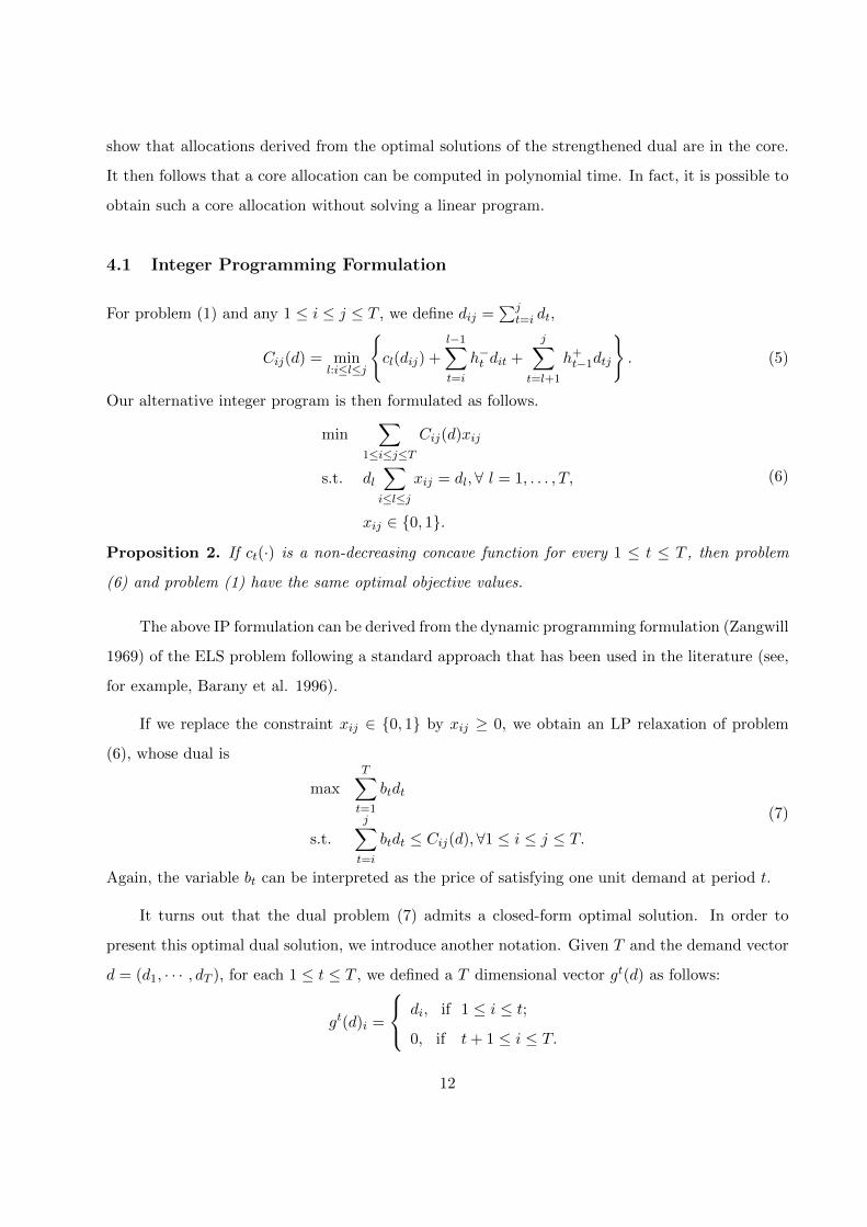
4.1 Integer Programming Formulation

For problem (1) and any 1 ≤ i ≤ j ≤ T , we define dij =∑j

t=i dt,

Cij(d) = minl:i≤l≤j

{cl(dij) +

l−1∑t=i

h−t dit +

j∑t=l+1

h+t−1dtj

}. (5)

Our alternative integer program is then formulated as follows.

min∑

1≤i≤j≤TCij(d)xij

s.t. dl∑i≤l≤j

xij = dl,∀ l = 1, . . . , T,

xij ∈ {0, 1}.

(6)

Proposition 2. If ct(·) is a non-decreasing concave function for every 1 ≤ t ≤ T , then problem

(6) and problem (1) have the same optimal objective values.

The above IP formulation can be derived from the dynamic programming formulation (Zangwill

1969) of the ELS problem following a standard approach that has been used in the literature (see,

for example, Barany et al. 1996).

If we replace the constraint xij ∈ {0, 1} by xij ≥ 0, we obtain an LP relaxation of problem

(6), whose dual is

maxT∑t=1

btdt

s.t.

j∑t=i

btdt ≤ Cij(d),∀1 ≤ i ≤ j ≤ T.(7)

Again, the variable bt can be interpreted as the price of satisfying one unit demand at period t.

It turns out that the dual problem (7) admits a closed-form optimal solution. In order to

present this optimal dual solution, we introduce another notation. Given T and the demand vector

d = (d1, · · · , dT ), for each 1 ≤ t ≤ T , we defined a T dimensional vector gt(d) as follows:

gt(d)i =

di, if 1 ≤ i ≤ t;

0, if t+ 1 ≤ i ≤ T.

12

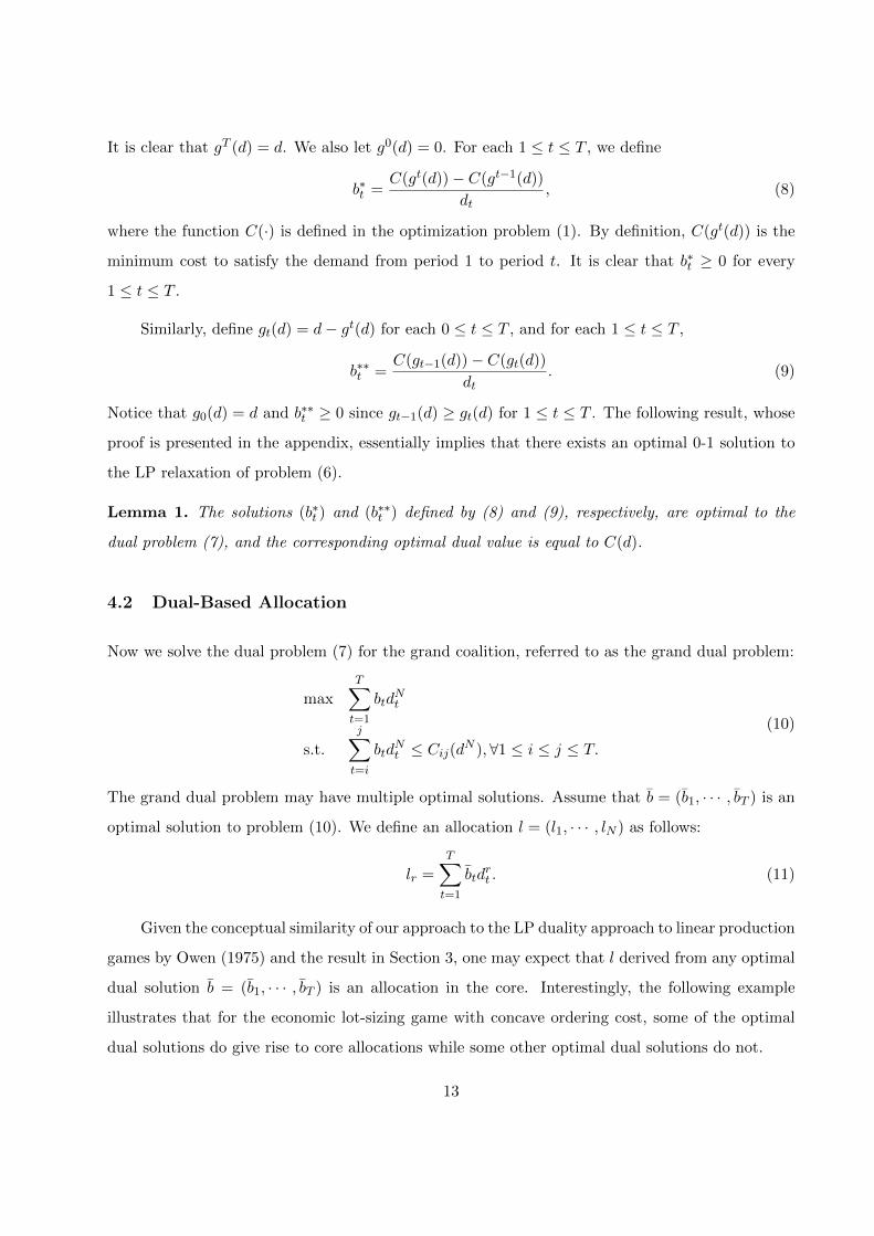
It is clear that gT (d) = d. We also let g0(d) = 0. For each 1 ≤ t ≤ T , we define

b∗t =C(gt(d))− C(gt−1(d))

dt, (8)

where the function C(·) is defined in the optimization problem (1). By definition, C(gt(d)) is the

minimum cost to satisfy the demand from period 1 to period t. It is clear that b∗t ≥ 0 for every

1 ≤ t ≤ T .

Similarly, define gt(d) = d− gt(d) for each 0 ≤ t ≤ T , and for each 1 ≤ t ≤ T ,

b∗∗t =C(gt−1(d))− C(gt(d))

dt. (9)

Notice that g0(d) = d and b∗∗t ≥ 0 since gt−1(d) ≥ gt(d) for 1 ≤ t ≤ T . The following result, whose

proof is presented in the appendix, essentially implies that there exists an optimal 0-1 solution to

the LP relaxation of problem (6).

Lemma 1. The solutions (b∗t ) and (b∗∗t ) defined by (8) and (9), respectively, are optimal to the

dual problem (7), and the corresponding optimal dual value is equal to C(d).

4.2 Dual-Based Allocation

Now we solve the dual problem (7) for the grand coalition, referred to as the grand dual problem:

maxT∑t=1

btdNt

s.t.

j∑t=i

btdNt ≤ Cij(dN ),∀1 ≤ i ≤ j ≤ T.

(10)

The grand dual problem may have multiple optimal solutions. Assume that b = (b1, · · · , bT ) is an

optimal solution to problem (10). We define an allocation l = (l1, · · · , lN ) as follows:

lr =T∑t=1

btdrt . (11)

Given the conceptual similarity of our approach to the LP duality approach to linear production

games by Owen (1975) and the result in Section 3, one may expect that l derived from any optimal

dual solution b = (b1, · · · , bT ) is an allocation in the core. Interestingly, the following example

illustrates that for the economic lot-sizing game with concave ordering cost, some of the optimal

dual solutions do give rise to core allocations while some other optimal dual solutions do not.

13

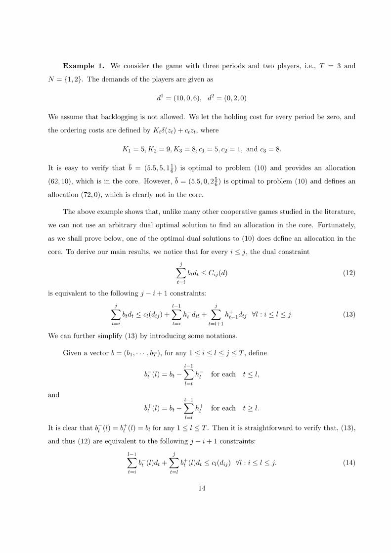
Example 1. We consider the game with three periods and two players, i.e., T = 3 and

N = {1, 2}. The demands of the players are given as

d1 = (10, 0, 6), d2 = (0, 2, 0)

We assume that backlogging is not allowed. We let the holding cost for every period be zero, and

the ordering costs are defined by Ktδ(zt) + ctzt, where

K1 = 5,K2 = 9,K3 = 8, c1 = 5, c2 = 1, and c3 = 8.

It is easy to verify that b = (5.5, 5, 116) is optimal to problem (10) and provides an allocation

(62, 10), which is in the core. However, b = (5.5, 0, 256) is optimal to problem (10) and defines an

allocation (72, 0), which is clearly not in the core.

The above example shows that, unlike many other cooperative games studied in the literature,

we can not use an arbitrary dual optimal solution to find an allocation in the core. Fortunately,

as we shall prove below, one of the optimal dual solutions to (10) does define an allocation in the

core. To derive our main results, we notice that for every i ≤ j, the dual constraint

j∑t=i

btdt ≤ Cij(d) (12)

is equivalent to the following j − i+ 1 constraints:

j∑t=i

btdt ≤ cl(dij) +

l−1∑t=i

h−t dit +

j∑t=l+1

h+t−1dtj ∀l : i ≤ l ≤ j. (13)

We can further simplify (13) by introducing some notations.

Given a vector b = (b1, · · · , bT ), for any 1 ≤ i ≤ l ≤ j ≤ T , define

b−t (l) = bt −l−1∑l=t

h−l for each t ≤ l,

and

b+t (l) = bt −t−1∑l=l

h+l for each t ≥ l.

It is clear that b−l (l) = b+l (l) = bl for any 1 ≤ l ≤ T . Then it is straightforward to verify that, (13),

and thus (12) are equivalent to the following j − i+ 1 constraints:

l−1∑t=i

b−t (l)dt +

j∑t=l

b+t (l)dt ≤ cl(dij) ∀l : i ≤ l ≤ j. (14)

14

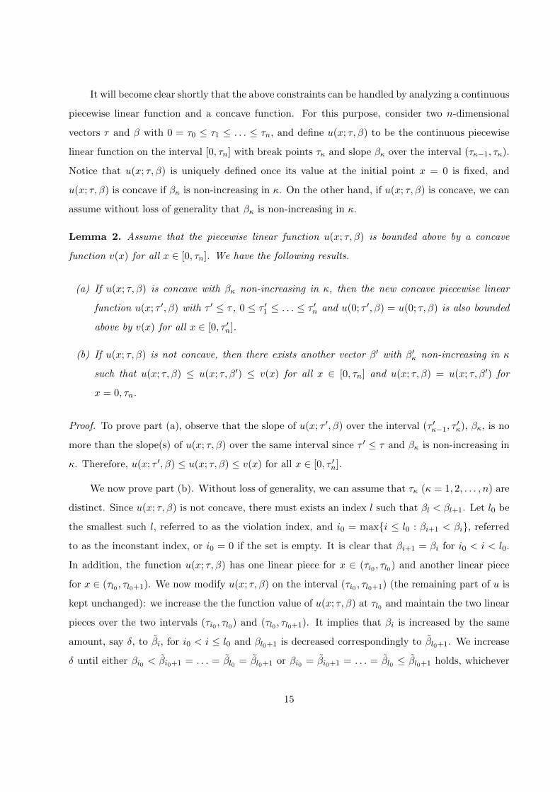
It will become clear shortly that the above constraints can be handled by analyzing a continuous

piecewise linear function and a concave function. For this purpose, consider two n-dimensional

vectors τ and β with 0 = τ0 ≤ τ1 ≤ . . . ≤ τn, and define u(x; τ, β) to be the continuous piecewise

linear function on the interval [0, τn] with break points τκ and slope βκ over the interval (τκ−1, τκ).

Notice that u(x; τ, β) is uniquely defined once its value at the initial point x = 0 is fixed, and

u(x; τ, β) is concave if βκ is non-increasing in κ. On the other hand, if u(x; τ, β) is concave, we can

assume without loss of generality that βκ is non-increasing in κ.

Lemma 2. Assume that the piecewise linear function u(x; τ, β) is bounded above by a concave

function v(x) for all x ∈ [0, τn]. We have the following results.

(a) If u(x; τ, β) is concave with βκ non-increasing in κ, then the new concave piecewise linear

function u(x; τ ′, β) with τ ′ ≤ τ , 0 ≤ τ ′1 ≤ . . . ≤ τ ′n and u(0; τ ′, β) = u(0; τ, β) is also bounded

above by v(x) for all x ∈ [0, τ ′n].

(b) If u(x; τ, β) is not concave, then there exists another vector β′ with β′κ non-increasing in κ

such that u(x; τ, β) ≤ u(x; τ, β′) ≤ v(x) for all x ∈ [0, τn] and u(x; τ, β) = u(x; τ, β′) for

x = 0, τn.

Proof. To prove part (a), observe that the slope of u(x; τ ′, β) over the interval (τ ′κ−1, τ′κ), βκ, is no

more than the slope(s) of u(x; τ, β) over the same interval since τ ′ ≤ τ and βκ is non-increasing in

κ. Therefore, u(x; τ ′, β) ≤ u(x; τ, β) ≤ v(x) for all x ∈ [0, τ ′n].

We now prove part (b). Without loss of generality, we can assume that τκ (κ = 1, 2, . . . , n) are

distinct. Since u(x; τ, β) is not concave, there must exists an index l such that βl < βl+1. Let l0 be

the smallest such l, referred to as the violation index, and i0 = max{i ≤ l0 : βi+1 < βi}, referred

to as the inconstant index, or i0 = 0 if the set is empty. It is clear that βi+1 = βi for i0 < i < l0.

In addition, the function u(x; τ, β) has one linear piece for x ∈ (τi0 , τl0) and another linear piece

for x ∈ (τl0 , τl0+1). We now modify u(x; τ, β) on the interval (τi0 , τl0+1) (the remaining part of u is

kept unchanged): we increase the the function value of u(x; τ, β) at τl0 and maintain the two linear

pieces over the two intervals (τi0 , τl0) and (τl0 , τl0+1). It implies that βi is increased by the same

amount, say δ, to βi, for i0 < i ≤ l0 and βl0+1 is decreased correspondingly to βl0+1. We increase

δ until either βi0 < βi0+1 = . . . = βl0 = βl0+1 or βi0 = βi0+1 = . . . = βl0 ≤ βl0+1 holds, whichever

15

happens first. In the former case, we increase the smallest violation index by 1, while in the latter

case, we decrease the inconstant index by 1. In either case, we can repeat the same process until

there is no more violation index. At this point, the resulting function u(x; τ, β′) must satisfy the

conditions in part (b). �

Lemma 3. Assume bt− h−t ≤ bt+1 ≤ bt + h+t for every 1 ≤ t ≤ T − 1. If (12) holds for d = dN for

any 1 ≤ i ≤ j ≤ T , then it also holds for any d = d′ ≤ dN .

Proof. It is clear that the assumption bt−h−t ≤ bt+1 ≤ bt+h+t for every 1 ≤ l ≤ T −1 is equivalent

to

b+t (l) ≥ b+t+1(l) for t ≥ l and b−t (l) ≤ b−t+1(l) for t ≤ l

for 1 ≤ l ≤ T .

For any i and l with i ≤ l, define

uil(x; d, b) =l−1∑k=i

b−k (l)dk +

j−1∑k=l

b+k (l)dk + b+j (l)(x− dl,j−1), for x ∈ [dl,j−1, dl,j ], j ≥ l, (15)

and

vil(x; d) = cl(di,l−1 + x). (16)

Our assumption implies that uil(x; d, b) is a concave piecewise linear function for x ∈ [0, dlT ] with

break points dlj (j = l, . . . , T ). In addition, uil(x; dN ) ≤ vil(x; dN ) for x = dlj (j = l, . . . , T ).

Therefore, uil(x; dN ) ≤ vil(x; dN ) for x ∈ [dNll , dNlT ]. For any vector d′ with d′j = dj for j = 1, . . . , l and

d′j ∈ [0, dNj ] for j > l, applying Lemma 2, we can show that uil(x; d′, b) ≤ vil(x; d′) for x ∈ [d′ll, d′lT ].

Similarly, for any j and l with j ≥ l, if we define

ujl (x; d, b) =

j∑k=l

b+k (l)dk +

l−1∑k=i+1

b−k (l)dk + b−i (l)(x− di+1,l−1), for x ∈ [di+1,l−1, di,l−1] (17)

and

vjl (x; d) = cl(x+ dlj), (18)

we can show that ujl (x; d′, b) ≤ vjl (x; d′) for x ∈ [0, d′1,l−1] for any vector d′ with d′i = di for i ≥ l

and d′i ∈ [0, dNj ] for i = 1, . . . , l − 1.

16

If dNi,l−1 ≥ dNl , we can define a new vector d′ such that d′i = di for i ≥ l, d′i ∈ [0, dNj ] for

i = 1, . . . , l − 1, and dNi,l−1 = d′i,l−1 + dNl . Our above discussion implies that

uil(0; dN , b) =∑l

k=i b−k (l)dk − b−l (l)dl

=∑l

k=i b−k (l)d′k +

∑l−1k=i(b

−k (l)− b−l (l))(dk − d′k)

≤ ull(d′i,l−1; d

′, b)

≤ vll(d′i,l−1; d

′)

= vil(0; dN ),

where the first inequality follows from the monotonicity of b−k (l) and the second inequality from

our above discussion. �

Lemma 4. Assume that b = (b1, · · · , bT ) is an optimal solution to problem (10). If bt − h−t ≤

bt+1 ≤ bt + h+t for every 1 ≤ t ≤ T − 1, then the allocation l = (l1, · · · , lN ) defined by

lr =

T∑t=1

btdrt

is in the core of the ELS game (N,F ).

Proof. Notice that for any S ⊆ N ,

∑r∈S

lr =∑r∈S

T∑t=1

btdrt =

T∑t=1

btdSt .

Therefore, by the definition of b,∑

r∈N lr is equal to the optimal value of (10), and thus equal to

F (N) by using Lemma 1.

It remains to show∑

r∈S lr ≤ F (S) for any S ⊆ N . By weak duality of linear programming,

it suffices to prove that b is feasible to

j∑t=i

btdSt ≤ Cij(dS),

which is implied by Lemma 3. The proof is complete. �

As stated in the lemma, the inequalities bt−h−t ≤ bt+1 ≤ bt +h+t for 1 ≤ t ≤ T − 1 are crucial

to our analysis, although by no means it is a necessary condition. We now provide some intuition

17

on these inequalities. Recall that the dual variable bi may be interpreted as the price of satisfying

one unit of demand at period i. Notice that the demand at period i+ 1 can be either satisfied by

orders after period i or by an order before period i + 1. In the latter case, period i + 1 demand

is satisfied by the inventory carried over from period i to period i + 1 by paying a unit inventory

holding cost h+i . Thus, it is reasonable to expect that the charge of a unit demand at period i+ 1

is no more than the charge of a unit demand at period i plus the unit inventory holding cost h+i .

The inequality bi+1 ≥ bi − h−i can be explained in a similar way.

The next question that we shall answer is whether or not there exists any optimal dual solution

that satisfies these inequalities. We first check whether or not the optimal solutions b∗ and b∗∗

defined by (8) and (9) satisfy these inequalities, and whether or not the cost allocations defined by

these optimal solutions are in the core.

Indeed, one can show that b∗t+1 ≤ b∗t + h+t for every t : 1 ≤ t ≤ T − 1 (we omit its proof here

as it is similar to the proof of Proposition 2 in Barany et al. (1984), and not crucial to our main

result). However, as illustrated by the following example, we may not have b∗t+1 ≥ b∗t −h−t for every

t : 1 ≤ t ≤ T − 1 and the cost allocation defined by b∗ may not be in the core.

Example 2. We consider a game with setup cost and three periods. Let the aggregated

demand d = (1, 5, 1). In addition, let

K = (2, 4, 1), c = (1, 0, 0), h+ = (1, 1, 0), h− = (1, 1, 0).

One can compute that b∗ = (3, 0.4, 1). It is straightforward to verify that b∗t+1 ≤ b∗t + h+t for every

t : 1 ≤ t ≤ T − 1. However, b∗2 < b∗1 − h−1 . We can also verify that b∗ = (3, 0.4, 1) is not feasible for

problem (3). Indeed, for t = 3,∑

1≤τ≤T dτ max(bτ − ptτ , 0) = 2 < 1 = Kt and thus it is impossible

to find {βtτ} such that b∗ = (3, 0.4, 1) is feasible for problem (3). Our discussion at the end of

Section 3 implies that there exists a demand profile such that the cost allocation induced by b∗ is

not in the core of the corresponding game.

Nonetheless, if backlogging is not allowed, then h−t = ∞ for every t. Thus, solution b∗ auto-

matically satisfies the condition required by Lemma 4. This leads to the following result

Corollary 2. If backlogging is not allowed, then the ELS game with non-decreasing concave cost

has a non-empty core. In particular, the allocation defined by (11) with b = b∗ is in the core.

18

Similarly, one can show that for solution b∗∗, b∗∗t+1 ≥ b∗∗t − h−t for every t : 1 ≤ t ≤ T − 1.

However, b∗∗t+1 ≤ b∗∗t + h+t may not hold for all t, and the cost allocation defined by b∗∗ may not be

in the core.

Even though b∗ and b∗∗ may not lead to core allocations, Lemma 5 below says that we can

always construct in polynomial time an optimal dual solution b, starting from either b∗ or b∗∗

(indeed any optimal dual solution for problem (7)), that satisfies the condition required by Lemma

4. The lemma is the key to our main result. It might be of independent interest as well.

Lemma 5. Given any feasible solution b = (b1, · · · , bT ) to problem (7), we can construct in poly-

nomial time another feasible solution b = (b1, · · · , bT ) with the same objective value such that

−h−t ≤ bt+1 − bt ≤ h+t for every t : 1 ≤ t ≤ T − 1.

The proof is carried out in two steps. In the first step, we construct a feasible solution b′

with the same objective value and b′t+1 ≤ b′t + h+t for every t : 1 ≤ t ≤ T − 1. In the second

step, we convert b′ to b with the same objective value such that −h−t ≤ bt+1 − bt ≤ h+t for every

t : 1 ≤ t ≤ T − 1. Both steps can be done in polynomial time. Notice that b∗ and b∗∗ can be

found in polynomial time via dynamic programming. Furthermore, if we start with solution b∗

(b∗∗ respectively), then we do not have to perform step 1 (step 2 respectively). Since the proof of

Lemma 5 is rather long, we present it in the appendix.

Lemma 5 and Lemma 4 immediate lead to our main result.

Theorem 2. For the ELS game (N,F ) with backlogging, and with general nondecreasing concave

ordering cost, linear inventory holding cost, and linear backlogging cost, the core is always non-

empty and an allocation in the core can be found in polynomial time.

In fact, we have picked a subset of the dual optimal solutions that lead to core allocations.

These solutions are the same as the optimal solutions to the following linear program.

maxT∑t=1

btdNt

s.t.

j∑t=i

btdNt ≤ Cij(dN ), ∀1 ≤ i ≤ j ≤ T

bt ≥ bt+1 − h+t , ∀1 ≤ t ≤ T − 1

bt ≤ bt+1 + h−t , ∀1 ≤ t ≤ T − 1

(19)

19

However, Lemma 5 and Lemma 4 imply that to find one of the core allocations, we do not really

need to solve the above linear program.

An interesting and open question is whether the core allocations derived from our approach

allow us to construct a population monotonic allocation scheme, which roughly speaking says that

adding one more player to the grand coalition reduces the cost allocations of existing players (see

Sprumont 1990 for the exact definition). Unfortunately, since problem (19) may have multiple

optimal solutions, it is not clear whether and how one can choose the optimal dual solutions

appropriately to construct a population monotonic allocation scheme.

Finally, we compare different formulations for the ELS game with setup cost. In this case,

both optimal solutions to (19) and (3) define allocations in the core. Let A1, A2, and A3 be the

sets of optimal solutions to problems (3), (10), and (19) with d = dN , respectively. We can show

that A3 $ A1 $ A2. The proof is straightforward and thus omitted.

5 Conclusion

In this paper, we study the ELS game with backlogging and with non-decreasing concave ordering

cost. We show that there exists an allocation in the core, which can be computed in polynomial

time.

There are several other directions for future research. First, our focus in this paper is the

core. However, there are several other important concepts in cooperative game such as the Shapley

value (Peleg and Sudholter 2003) and the nucleolus (Deng and Papadimitriou 1994). It would be

interesting to design efficient algorithms to compute them.

Second, we have essentially assumed that the retailers have uniform inventory holding costs.

In addition, the inventory holding cost and backlogging cost are assumed to be linear functions.

We are currently investigating whether some of these assumptions can be relaxed.

Third, the demand is assumed to be exogenous in this paper. However, in many practical

situations, demand could be a function of the price of the product, and the price can be optimized,

together with inventory decisions, in order to maximize profit (see, for instance, Chen and Simchi-

Levi 2004a, 2004b). It remains a challenge to incorporate pricing decisions into ELS games.

20

Finally, we hope the methodology employed here can encourage more research developing

effective cost allocation mechanisms essential for sustainable collaborations in many not for profit

operations.

Acknowledgement. We thank Professor A. Tamir for helpful discussions on the topic of this paper

and for bringing the paper Tamir (1992) to our attention. We also thank Professor G. Shanthikumar

and the anonymous referees for insightful comments and suggestions. The research of Xin Chen

was partly supported by the National Science Foundation Grants CMMI-0653909, CMMI-0926845

ARRA and CMMI-1030923, CMMI-1363261, CMMI-1538451 and National Science Foundation of

China (NSFC) Grants 71520107001 and 71228203, and the research of Jiawei Zhang was partly

supported by National Science Foundation Grant CMMI-0654116.

References

Anily, S. and Haviv, M. 2007. The Cost Allocation Problem for the First Order Interaction Joint

Replenishment Model. Operations Research, 55 (2), pp. 292-302.

Arikan, E., Sigala, I., Silbermayr, L., Jammernegg, W., and Toyasaki, F. 2015. Disaster relief

inventory management: horizontal cooperation between humanitarian organizations. Working pa-

per.

Armed Services Board of Contract Appeals No. 58587.

(http://www.asbca.mil/Decisions/2013/58587 The Boeing Company 12.3.13 PUBLISHED.pdf)

Barany, I., Van Roy, T., and Wolsey, L.A. 1984. Uncapacitated lot-sizing: the convex hull of

solutions. Mathematical Programming Study, 22, pp. 32-43.

Barany, I., Edmonds, J., and Wolsey, L.A. 1986. Packing and covering a tree by subtrees. Combi-

natorica, 6, pp. 221-233.

Chen, X. 2009. Inventory Centralization Games with Price-Dependent Demand and Quantity

Discount. Operations Research, 57 (6), pp. 1394-1406.

21

Chen, X. and D. Simchi-Levi. 2004a. Coordinating Inventory Control and Pricing Strategies with

Random Demand and Fixed Ordering Cost: The Finite Horizon Case. Operations Research, 52

(6), pp. 887-896.

Chen, X. and D. Simchi-Levi. 2004b. Coordinating Inventory Control and Pricing Strategies with

Random Demand and Fixed Ordering Cost: The Infinite Horizon Case. Mathematics of Operations

Research, 29 (3), pp. 698-723.

Chen, X. and Zhang, J. 2009. A stochastic programming duality approach to inventory central-

ization games. Operations Research, 57 (4), pp. 840-851.

Deng, X. and Papadimitriou, C.H. 1994. On the complexity of cooperative solution concepts.

Mathematics of Operations Research, 19, pp. 257–266

Dror, M. and Hartman, B. 2007. Shipment Consolidation: Who pays for it and how much. Man-

agement Science, 53, pp. 78-87.

Feigenbaum, J. and Papadimitriou, C. and Shenker, S. 2000. Sharing the cost of muliticast trans-

missions (preliminary version). STOC ’00: Proceedings of the thirty-second annual ACM sympo-

sium on Theory of computing, 218-227.

Faigle, U., W. Kern, S. P. Fekete and W. Hochstattler 1997. On the complexity of testing mem-

bership in the core of min-cost spanning tree games, Int. J. Game Theory, 26, pp. 361–366.

Goemans, M.X. and Skutella, M. 2004. Cooperative facility location game. Journal of Algorithms,

50(2), pp. 194–214.

Gopaladesikan, M., Uhan, N., and Zou, J. 2012. A primaldual algorithm for computing a cost

allocation in the core of economic lot-sizing games. Operations Research Letters, 40(6), pp. 453–

458.

Granot D. 1986. A generalized linear production model: A unifying model. Mathematical Pro-

gramming, 34(2), pp. 212–222.

Gui, L., Atasu, A., Ergun, O., and Toktay, B. 2014 Fair and Efficient Implementation of Collective

Extended Producer Responsibility Legislation. Management Science, forthcoming.

22

Krarup J. and Bilde, O. 1977. Plant location, set covering and economic lot sizing: an O(mn)

algorithm for structural problems. In Numerische Methoden Bei Optimierungsaufgaben, volume

3, pp. 55–180.

Mahdian, M., Ye, Y. and Zhang, J. 2006. Approximation Algorithms for Metric Facility Location

Problems. SIAM Journal on Computing, Vol. 36, No. 2, pp. 411-432.

Manne, A.S. 1958. Programming of dynamic lot sizes. Management Science, 4, 115–135.

Muller, A., Scarsini, M. and Shaked, M. 2002. The newsvendor game has a non-empty core. Games

and Economic Behavior, 38, pp. 118–126.

Owen, G. 1975. On the core of linear production games. Mathematical Programming, 9, pp. 358–

370.

Peleg, B. and Sudholter, P. 2003. Introduction to the Theory of Cooperative Games. Kluwer Aca-

demic Publishers, Boston.

Pochet, Y. and Wolsey, L.A. 1988. Lot-size models with backlogging: Strong reformulations and

cutting planes. Mathematical Programming, 40, pp. 317-335.

Samet, D. and Zemel, E. 1984. On the core and dual set of linear programming games, Mathematics

of Operations Research, 9, 309–316.

Shapley, L.S. 1967. On balanced sets and core. Naval Res. Logist. Quart., 14, pp. 453-460.

Shubik, M. 1962. Incentives, decentralized control, the assignment of joint costs and internal

pricing. Management Science, 8(3), 325-343.

Sprumont, Y. 1990. Population montonic allocation schemes for cooperative games with transfer-

able utility. Games and Economic Behavior, 2, pp. 378–394.

Tamir, A. 1991. On the core of network synthesis games. Mathematical Programming, 50, pp.

123–135.

Tamir, A. 1992. On the core of cost allocation games defined on location problems. Transportation

Science, 27(1), pp. 81–86.

23

Toriello, A. and Uhan, N. 2014. Dynamic cost allocation for economic lot sizing games. Operations

Research Letters, 42(1), pp. 82-84.

van den Heuvel. 2008. Private communication.

Van Hoesel, C.P.M., Wagelmans, A., and Kolen, A. 1991. A dual algorithm for the economic

lot-sizing problem. European Journal of Operational Research, 52, pp. 315-325.

Wagner, H.M. and Whitin, T.M. 1958. Dynamic version of the economic lot size model. Manage-

ment Science, 5, pp. 89–96.

WHO website on vaccine procurement. Retrieved December 12, 2015.

(http://www.who.int/immunization/programmes systems/procurement/mechanisms systems

/pooled procurement/en/index1.html)

Young, H. P., N. Okada, and T. Hashimoto. 1982. Cost Allocation in Water Resources Develop-

ment. Water Resource Research, 18(3), 463-475.

Zangwill, W.I. 1969. A Backlogging Model and a Multi-Echelon Model of a Dynamic Economic

Lot Size Production System-A Network Approach. Management Science, 15(9), pp. 506-527.

Zhang, J.W. 2009. Cost Allocation for Joint Replenishment Models. Operations Research, 57 (1),

pp. 146-156.

Zolezzi, J. M. and Rudnick, H. 2002. Transmission cost allocation by cooperative games and

coalition formation. IEEE Transactions on Power Systems, 17(4), 1008-1015.

Appendix

Proof of Lemma 1.

We will show that (b∗t ) is optimal to problem (7). The proof of the optimality of (b∗∗t ) is similar.

First of all, we show that (b∗t ) is a feasible solution to problem (7). To that end, we notice that for

24

any 1 ≤ i ≤ j ≤ d,

j∑t=i

b∗tdt =

j∑t=i

C(gt(d))− C(gt−1(d))

= C(gj(d))− C(gi−1(d))

≤ Cij(d),

where the last inequality holds since

C(gj(d)) ≤ C(gi−1(d)) + Cij(d), (20)

which in turn follows from the fact that the right hand side of (20) is the cost of a feasible ordering

policy to satisfy the demand from period 1 to period j (i.e., by ordering optimally to satisfy the

demand from period 1 and period i− 1, and ordering at a period in between i and j to satisfy the

total demand from period i to period j), while the left hand side of (20) is the minimum cost to

achieve that.

Moreover, the objective value of problem (7) associated with the solution (b∗t ) is

T∑t=1

b∗tdt = C(gT (d)) = C(d),

which is the optimal objective value of the integer program (6). Then it follows from the weak

duality of LP, (b∗t ) must be an optimal solution to problem (7) with an objective value of C(d).

Proof of Lemma 5

For a given function f : < → <, define its left-side directional derivative as

f ′−(x) = limδ→0−

f(x+ δ)− f(x)

δ.

Then we have,

Lemma 6. Assume that u, v : X ⊂ < → < are two functions on an interval X and u(x) ≤ v(x)

for any x ∈ X. Then for any x with u(x) = v(x), u′−(x) ≥ v′−(x) as long as x is different from X’s

left end point and the directional derivatives are well defined.

The proof of Lemma 6 is straightforward and thus omitted.

25

Given a feasible solution b = (b1, · · · , bT ) to problem (7), we convert b = (b1, · · · , bT ) to another

feasible solution b = (b1, · · · , bT ) with the same objective value such that −h−t ≤ bt+1− bt ≤ h+t for

every 1 ≤ t ≤ T − 1.

Though the proof is lengthy, the idea is similar to the observation made in Lemma 2 part

(b). The additional complexity comes from the fact that we have to maintain several inequalities

simultaneously while changing both the function values at the initial point and the slopes of the

relevant piecewise linear functions.

To simplify our analysis, we first assume that dj > 0 for j = 1, . . . , T .

Assume that there exists some t such that h−t ≤ bt+1 − bt ≤ h+t is violated. Let l0 be the

violation index, i.e., the smallest such t. We will show that we can change the values of bi for

i ≤ l0 + 1 so that the violation index will increase by at least 1. In addition, the new solution is

still feasible with the objective value unchanged.

We distinguish between two different cases.

Case 1. bl0+1 > bl0 + h+l0 .

Let i0 be the inconstant index, i.e.,i0 = max{i ≤ l0 : bi+1 − bi < h+i } or i0 = 0 if the set is

empty. It is clear that i0 + 1 ≤ l0. Furthermore, for any i0 + 1 ≤ i < l0, bi+1− bi = h+i . For a given

δ > 0, we define b such that for every j,

bj =

bj + δ, if i0 + 1 ≤ j ≤ l0;

bj −di0+1,l0dl0+1

δ, if j = l0 + 1;

bj , otherwise.

(21)

It is clear that b and b have the same objective value. We shall show that there exists some small

δ > 0 such that b is feasible. That is, for any i ≤ l ≤ j,

l−1∑k=i

b−k (l)dk +

j∑k=l

b+k (l)dk ≤ cl(dij), (22)

where b−k (l) = bk −∑l−1

t=k h−k for k ≤ l − 1 and b+k (l) = bk −

∑j−1t=k h

+k for k ≥ l.

If l > l0, or j ≤ i0, or l ≤ l0 and j ≥ l0 + 1, the inequality (22) obviously holds for b. Thus, we

assume that max(l, i0 + 1) ≤ j ≤ l0.

Recall the functions uil(x; d, b) and vil(x; d) defined in (15) and (16). For simplicity, denote

26

uil(x) = uil(x; d, b) and vil(x) = vil(x; d). Since the vector b is feasible, we have that uil(x) ≤ vil(x)

for any x = dlj (j = l, . . . , T ) and i ≤ l. On the other hand, the definition of l0 implies that

b−1 (l) ≤ b−2 (l) ≤ b−l (l) and thus uil(0) ≤ vil(0) from the proof in Lemma 3. Since uil is piecewise

linear with break points dlk (k = l, . . . , T ) and vil is concave, we have that uil(x) ≤ vil(x) for any

x ∈ [0, dlT ] and i ≤ l.

To define δ, we claim that uil(dlj) < vil(dlj) for any i ≤ l ≤ max(l, i0 + 1) ≤ j ≤ l0. Otherwise,

there must exist i, l, j such that i ≤ l ≤ max(l, i0 + 1) ≤ j ≤ l0 and uil(dlj) = vil(dlj). Then by

Lemma 6,

b+j (l) =

{duil−(x)

dx

}|x=dlj ≥

{dvil−(x)

dx

}|x=dlj ≥

dvil−(x)

dx, for x ∈ [dlj , dlT ], (23)

where the second inequality follows from the concavity of function vil(x). On the other hand, it is

clear that

b+l0+1(l) > b+l0(l) = b+j (l). (24)

Since the function uil(x) is linear in (dl,j−1, dl,l0 ] with a slope of b+l0(l) and linear in (dl,l0 , dl,l0+1] with

a slope of b+l0+1(l), and vil(x) is concave, (23) and (24) imply that uil(x) > vil(x) for x ∈ (dl,j , dl,l0+1],

which contradicts the feasibility of b. Thus, uil(dlj) < vil(dlj) for any i ≤ l ≤ max(l, i0 + 1) ≤ j ≤ l0.

We can now choose δ such that

δ = min

{min

i,l,j:i≤l≤max(l,i0+1)≤j≤l0

vil(dlj)− uil(dlj)dmax(i,i0+1),j

, (bl0+1 − bl0 − h+l0

)dl0+1

di0+1,l0+1, bi0 + h+i0 − bi0+1

}> 0,

(25)

if i0 ≥ 1, and

δ = min

{min

i,l,j:i≤l≤max(l,i0+1)≤j≤l0

vil(dlj)− uil(dlj)dmax(i,i0+1),j

, (bl0+1 − bl0 − h+l0

)dl0+1

di0+1,l0+1

}> 0,

if i0 = 0.

From our construction, we have that b satisfies (22) and thus is still feasible to problem (7).

Since δ ≤ (bl0+1 − bl0 − h+l0

)dl0+1

di0+1,l0+1, we have bl0+1 ≥ bl0 + h+l0 and therefore bi+1 ≥ bi − h−i for

i ≤ l0.

If δ = mini,l,j:i≤l≤max(l,i0+1)≤j≤l0vil (dlj)−u

il(dlj)

dmax(i,i0+1),j, we claim that b+1 (1) ≥ . . . ≥ b+l0(1) = b+l0+1(1).

If this is not true, it is clear that l0 is the violation index associated with b, i.e., the smallest

l such that b+l+1(1) > b+l (1). Similar to the argument we used before, we can show that for

27

i ≤ l ≤ max(l, i0 + 1) ≤ j ≤ l0, uil(dlj) < vil(dlj), where in the definition of ujl (·), b is replaced by b.

But this contradicts the definition of δ.

If δ = b+i0(1) − b+i0+1(1), then b+i0(1) = b+i0+1(1) = . . . = b+l0(1). Therefore, inconstant index

is decreased by at least one. In this case, if l0 remains the violation index for b, we repeat the

above argument by at most i0 times and each time the value of i0 will be reduced by at least one.

Eventually, we end up with b+1 (1) ≥ . . . ≥ b+l0(1) = b+l0+1(1).

Case 2. bl0+1 < bi0 − h−l0 .

Let i0 be the inconstant index, i.e.,i0 = max{i ≤ l0 : bi+1 − bi > −h−i } or i0 = 0 if the set is

empty. It is clear that i0 + 1 ≤ l0. Furthermore, for any i0 + 1 ≤ i < l0, bi+1 − bi = −h−i . For a

given δ > 0, we define b such that for every j,

bj =

bj − δ, if i0 + 1 ≤ j ≤ l0;

bj +di0+1,l0dl0+1

δ, if j = l0 + 1;

bj , otherwise.

(26)

It is clear that b and b have the same objective value. We shall show that there exists some small

δ > 0 such that b is feasible, i.e., for any i ≤ l ≤ j, inequality (22) holds.

If l ≤ l0, or i > j0, or l > l0 and i ≤ l0, the inequality (22) obviously holds for b. Thus, we

assume that l0 + 1 ≤ i ≤ min(j0, l). It is clear that we can simply focus on i with di > 0.

We know that ujl (x) ≤ vjl (x) for any x ∈ [0, d1,l−1], where for simplicity, denote ujl (x) =

ujl (x; d, b) and vjl (x) = vjl (x; d), with ujl and vjl being defined in (17) and (18), respectively. To

define δ, we claim that ujl (di,l−1) < vjl (di,l−1) for any l0 + 1 ≤ i ≤ min(j0, l). Otherwise, assume

that there exists i, l, and j such that ujl (di,l−1) = vjl (di,l−1). Then we can show, similar to (23) and

(24),

b−l0 > b−l0+1 = b−i =

{dujl−(x)

dx

}|x=dil−1

≥

{dvjl−(x)

dx

}|x=di,l−1

≥dvjl−(x)

dx, for x ∈ [di,l−1, d1,l−1].

This implies that ujl (x) > vjl (x) for x ∈ (di,l−1, dl0+1,l−1], which contradicts the feasibility of b.

Thus, ujl (di,l−1) < vjl (di,l−1) for any l0 + 1 ≤ i ≤ min(j0, l). We can now choose δ such that

δ = min

{min

i,l,j:l0+1≤i≤min(j0,l)≤l≤j

vjl (di,l−1)− ujl (di,l−1)

dl0+1,min(j0,l),−(bl0+1 − bl0 + h−l0)

dl0dl0,j0

, bj0+1 − bj0 + h−j0

}> 0,

28

if j0 < T , and

δ = min

{min

i,l,j:l0+1≤i≤min(j0,l)≤l≤j

vjl (di,l−1)− ujl (di,l−1)

dl0+1,min(j0,l),−(bl0+1 − bl0 + h−l0)

dl0dl0,j0

}> 0

if j0 = T . Then b satisfies (22) and thus is still feasible to problem (7).

Now we consider two cases.

Case 1. δ = −(bl0+1 − bl0 + h−l0)dl0dl0,j0

. In this case, we have that bl0+1 = bl0 − h−l0

. Therefore,

the largest integer such that bt+1 < bt − h−t has decreased by at least 1. This is exactly what we

need.

Case 2. δ < −(bl0+1 − bl0 + h−l0)dl0dl0,j0

. In this case, bl0+1 < bl0 − h−l0

. It implies that l0 is the

largest integer such that bt+1 < bt−h−t . Then by the same argument as above, ujl (di,l−1) < vjl (di,l−1)

for any l0 + 1 ≤ i ≤ min(j0, l), where in the definition of ujl (·) and vjl (·), we replace b with b. This

would imply that δ <vjl (di,l−1)−ujl (di,l−1)

dl0+1,min(j0,l). It then follows that δ = bj0+1 − bj0 + h−j0 . Hence we

have b−j0+1 = · · · = b−j0 . Therefore, the value of min{j ≥ l0 + 1 : bj+1 − bj > −h−j } is no less than

j0 + 1. We can repeat the procedure by at most T − j0 times until Case 2 will not happen (and

thus eventually we are in Case 1).

The only thing that is left to verify is that bt+1 ≤ bt + h+t for every 1 ≤ t ≤ T − 1. This

inequality can possibly be violated if during the process one of the following situations happens.

(Notice that for the variables increased, they are increased by the same amount.)

(1) bt+1 is increased by δ, but bt is unchanged, or bt is unchanged, but bt−1 is decreased by a

positive amount. It is clear that this can never happen in our procedure.

(2) bt+1 is increased by δ, but bt is decreased by a positive amount. This happens only if

t = l0. But after the change, bl0+1 = bl0+1 + δ, and bl0 = bl0 −dl0+1,j0dl0

δ. By the definition of δ,

bl0+1 = bl0 − h−l0

and thus bl0+1 ≤ bl0 + h+l0 .

We now illustrate the above procedure on Example 2 starting with b = b∗ = (3, 0.4, 1). As

we already pointed out, only Step 2 is needed. In this case, it is easy to see that l0 = 1 and

j0 = 2. Careful calculation gives δ = 0.8/3 = −(b2 − b1 + h−1 ) d1d12 and b = (53 ,23 , 1). Clearly,

−h−t ≤ bt+1 − bt ≤ h+t for t = 1, 2.

29