Lot-sizing Algorithms in Flexible Manufacturing Systems

81

Volume 25, November 2019

Asst. Prof. Chairat Hiranyavasit, Ph.D.*

Abstract

A flexible manufacturing system (FMS) is a manufacturing system for producing goods that is

readily adaptable to changes in the product being manufactured, both in type and quantity. Machines

and computerized systems are configured to manufacture different parts and handle varying levels of

production. This research focuses on lot-sizing decisions which are critical to the successful implementation

and operations of FMS. The objectives of the research are to explore how some of the traditional lot-sizing

algorithms currently available in the job shop production systems may be modified to accommodate

the unique characteristics and operating environments of FMS, and to conduct a series of simulation

experiments to evaluate the performance of the proposed lot-sizing algorithms in hypothetical FMS

under a selected set of operating conditions.

Keywords: Lot sizing, Flexible Manufacturing Systems, Simulation Experiments

* NIDA Business School, National Institute of Development Administration (NIDA), Bangkok, Thailand.

Lot-sizing Algorithms in Flexible Manufacturing Systems with Simulation Experiments

Received: June 21, 2019 / Accepted: August 23, 2019

Lot-sizing Algorithms in Flexible Manufacturing Systems with Simulation Experiments, P.81-99ISSN 1905-6826Journal Homepage :

http://mba.nida.ac.th

82

เลมท 25 พฤศจกายน 2562

ผศ.ดร.ชยรช หรญยะวะสต*

บทคดยอ

ระบบการผลตแบบยดหยน เปนระบบการผลตทสามารถปรบเปลยนตวเองเพอสามารถรองรบการผลตสนคาทม

การเปลยนแปลงทงในเชงประเภทและปรมาณ เครองจกรและระบบคอมพวเตอรจะถกน�ามาใชในระบบการผลตใหท�างาน

ประสานกน ทจะท�าใหสามารถผลตชนสวนทแตกตางกนในปรมาณการผลตทไมคงท งานวจยนเกยวของกบการตดสนใจ

ก�าหนดปรมาณการผลต ซงมความส�าคญมากในการน�าระบบการผลตแบบยดหยนมาใชไดอยางประสบความส�าเรจ งานวจยน

มเปาหมายเพอดดแปลงอลกอรทมในการก�าหนดปรมาณการผลตทใชในระบบการผลตแบบจอบชอปใหสามารถน�ามาใชใน

ระบบการผลตแบบยดหยนทมสภาพการผลตทแตกตางออกไป และท�าการทดลองประสทธภาพการใชงานของอลกอรทม

ในโมเดลจ�าลองการผลตแบบยดหยนในสภาพการผลตทแตกตางกน

ค�ำส�ำคญ: การก�าหนดปรมาณการผลต ระบบการผลตแบบยดหยน

อลกอรทมในกำรค�ำนวณปรมำณกำรผลตในระบบกำรผลตแบบยดหยนพรอมกำรทดลองในโมเดลกำรผลตแบบจ�ำลอง

* คณะบรหารธรกจ สถาบนบณฑตพฒนบรหารศาสตร

83


Introduction

In the field of operations management, a flexible manufacturing system (FMS) is one of the areas

that has gained considerable interest and attention from both practitioners and researchers. The design of

FMS follows the conceptual idea of group technology (GT) to explore the similarities which exist among

component parts produced in the machine shops so that production efficiencies and productivity can

be improved (Arn, 1975; Burbidge, 1975, 1979; DeVries, Harvey & Tipnis, 1976; Edwards, 1971; Gallagher

& Night, 1973; Ham, Hitomi & Yoshida, 1985; Hyer, 1984a, 1984b; Hyer, Wemerlov & Hyer, 1982, 1984;

Mitrofanov, 1966; Petrov, 1966, 1968; Ranson, 1972; Wemmerlov & Hyer, 1987a). The group technology

philosophy has broad applications such as the organization of component parts into part-families and

the organization of machines into manufacturing cells. The organization of component parts into

part-families can be done on either the basis of design or manufacturing process similarities or both.

When the organization of part-families is done by design similarity, the benefits are that new part

designs and component part variety may be reduced, and part standardization may be improved.

When part-families are organized based on manufacturing process similarity, the impact is upon the

structure or layout of production process itself.

The manufacturing of small and medium-sized batches of component parts has traditionally

taken place in a functional or job shop system where functionally similar machines are placed together

in a work center. Thus, batches of component parts must be moved through various work centers

according to a pre-specified sequence of operations. The group technology can be applied in production

process designs in various ways, but the extreme application of group technology to batch production

involves a physical rearrangement of machines and processes in a production system. Instead of organizing

a production system around machine similarity, groups of different machines on which a part-family

or a set of part-families may be produced are identified and placed together to form a production or

manufacturing cell. Each manufacturing cell is then dedicated to the manufacture of those part-families.

This type of manufacturing systems is commonly referred to as cellular manufacturing systems (CMS)

and flexible manufacturing systems (FMS).

Statement of the Problem

This research examines the production planning and control aspect of FMS. Specifically, it focuses

on the lot-sizing decisions which are critical in achieving high efficiency and productivity in manufacturing

systems. The rational for the need for studying the lot-sizing problems in FMS is that most of the lot-sizing

research has focused on job shops but the characteristics and production environments of FMS are

quite different from those found in job shops. Some of these different characteristics are:

84


(1) Component parts in FMS are grouped into part-families according to their design or

manufacturing similarity.

(2) Machines and operating processes in FMS are also grouped together to form manufacturing

cells so that a certain set of part families can be completely processed within each cell.

(3) In many circumstances especially when part-families are formed on the basis of their setup

requirement similarity, FMS provides an opportunity to reduce setup times by organizing the

setup requirements into major setup and minor setups. Major setups in FMS stem from changes

in the production from one part-family to another, whereas minor setups stem from changes

from one component part to another within the same part-family. Therefore, if component parts

which belong to the same part family are scheduled together, the overall setup times can

be reduced.

Because of the unique characteristics and production conditions of FMS, an argument can be

made that traditional lot-sizing procedures commonly used in job shops may not generate good and

acceptable results in FMS. The major questions to be asked are: How can lot-sizing decisions be made in

FMS? Can traditional lot-sizing procedures currently available in most of production planning and control

systems, such as Material Requirement Planning (MRP) systems, be modified for use in FMS environments?

If so, what modifications should or can be made? How beneficial are these modifications?

Objectives of the Research

This research has two main objectives. The first objective is to explore how some traditional

lot-sizing procedures commonly used in job shops can be modified to accommodate the unique

characteristics and operating conditions of FMS.

The second objective of this research is to conduct a series of simulation experiments to test the

performance of lot-sizing algorithms proposed in the research in a variety of FMS operating conditions.

Scope of the Research

This research focuses on finding ways to modify selected traditional lot-sizing procedures

commonly used in commercialized MRP system to accommodate the unique characteristics of FMS.

Two traditional lot-sizing procedures are selected for this study including period order quantity procedure

and Silver-Meal procedure. Even though there may be other traditional lot-sizing procedures which can

be modified to accommodate the unique characteristics of FMS, the previous two lot-sizing procedure

are selected because they are well-known in industries and modifications to the original procedures

are simple and minimal.

Since it is impractical to test the new lot-sizing algorithms in real world, the lot-sizing algorithms

proposed in this study were tested in a hypothetical FMS. A simulation model was developed to represent

85


a hypothetical FMS and a series of simulation experiments is conducted to test the performance of

the proposed lot-sizing algorithms.

Expected Contributions of the Research

It is expected that the results of this research will contributions to theoretical advancements on

the areas of production planning and scheduling in the FMS environment, especially in solving lot-sizing

problems. Some industries may benefit from this research such as flexible manufacturing systems for

producing component parts in automotive, electronic, and home appliance industries.

Literature Review

Most researchers studying lot-sizing problems in cellular and flexible manufacturing environments

have adopted an idea that since major setup times in cellular manufacturing stem from changes in

part-families and not from changes within part-families, therefore, lot-sizing in cellular manufacturing

should be done by part-families rather than by individual parts.

One group of researchers (Burbidge, 1975; Levulis, 1978; New, 1977; Suresh, 1979) has suggested

the use of single-cycle, single-phase ordering (also known as “Period Batch Control” or “PBC”) approach

to determine lot sizes by part-families. With this approach, all parts are ordered with a frequency

determined by the common production cycle, and parts scheduled for production in each cycle are then

categorized by families. In fact, the PBC approach is similar to the LFL procedure in MRP systems with the

size of planning time bucket set equal to the common planning cycle. Surprisingly, no formal method

for determining a proper planning cycle length has been proposed in the PBC literature.

Fogarty and Barringer (1984, 1987) considered the family lot-sizing problem as one of deciding

which parts to be included in an order to minimize costs (i.e., joint order replenishment problem).

They proposed a least total cost (LTC) approach and a dynamic programming approach for solving this

problem. However, their least total cost approach is impractical for use since this approach requires a trial

and error technique to examine a large number of the possible solutions. Their dynamic programming

approach also has a limitation in that it can only be used in the case of a single part-family produced

on non-dedicated machines.

Rabbi and Lakhmani (1984) conducted simulation experiments to investigate the performance

of an MRP-based specifically for their study and a family-oriented LTC lot-sizing procedure like the one

proposed by Fogarty and Barringer (1984). The results of their experiments show that the modified MRP

system with the family-oriented LTC lot-sizing procedure outperforms the standard MRP system with

the traditional LTC procedure in terms of inventory setup time to total individual setup times is low and

the number of parts in a part-family is large.

86


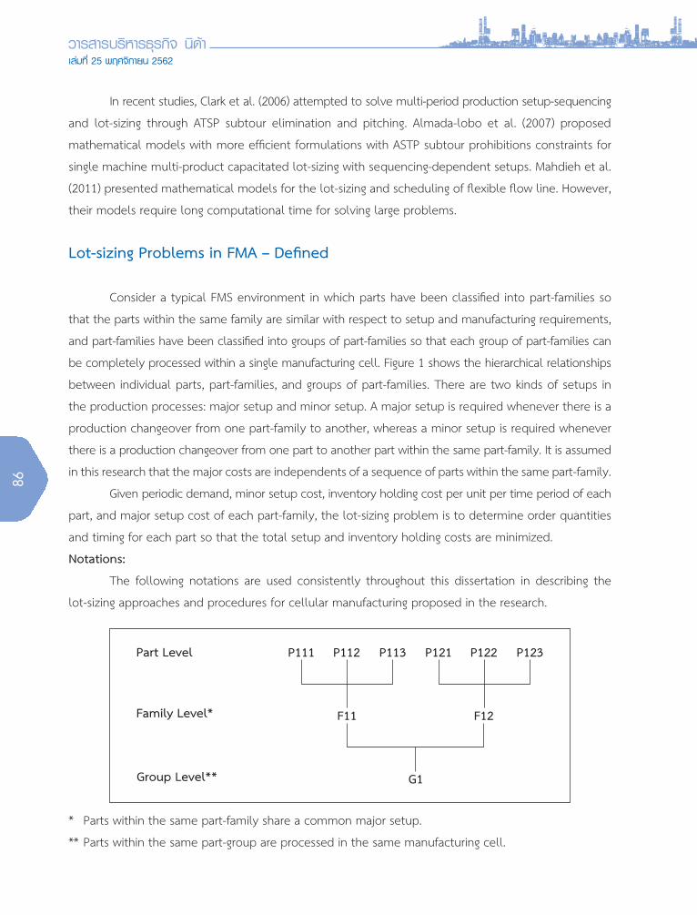
* Parts within the same part-family share a common major setup.

** Parts within the same part-group are processed in the same manufacturing cell.

In recent studies, Clark et al. (2006) attempted to solve multi-period production setup-sequencing

and lot-sizing through ATSP subtour elimination and pitching. Almada-lobo et al. (2007) proposed

mathematical models with more efficient formulations with ASTP subtour prohibitions constraints for

single machine multi-product capacitated lot-sizing with sequencing-dependent setups. Mahdieh et al.

(2011) presented mathematical models for the lot-sizing and scheduling of flexible flow line. However,

their models require long computational time for solving large problems.

Lot-sizing Problems in FMA – Defined

Consider a typical FMS environment in which parts have been classified into part-families so

that the parts within the same family are similar with respect to setup and manufacturing requirements,

and part-families have been classified into groups of part-families so that each group of part-families can

be completely processed within a single manufacturing cell. Figure 1 shows the hierarchical relationships

between individual parts, part-families, and groups of part-families. There are two kinds of setups in

the production processes: major setup and minor setup. A major setup is required whenever there is a

production changeover from one part-family to another, whereas a minor setup is required whenever

there is a production changeover from one part to another part within the same part-family. It is assumed

in this research that the major costs are independents of a sequence of parts within the same part-family.

Given periodic demand, minor setup cost, inventory holding cost per unit per time period of each

part, and major setup cost of each part-family, the lot-sizing problem is to determine order quantities

and timing for each part so that the total setup and inventory holding costs are minimized.

Notations:

The following notations are used consistently throughout this dissertation in describing the

lot-sizing approaches and procedures for cellular manufacturing proposed in the research.

87


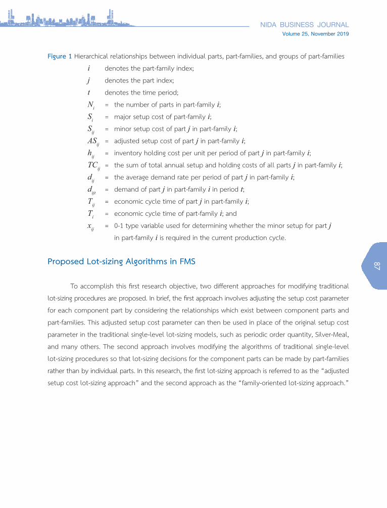
Figure 1 Hierarchical relationships between individual parts, part-families, and groups of part-families

i denotes the part-family index;

j denotes the part index;

t denotes the time period;

Ni = the number of parts in part-family i;Si = major setup cost of part-family i;Sij = minor setup cost of part j in part-family i;ASij = adjusted setup cost of part j in part-family i;hij = inventory holding cost per unit per period of part j in part-family i;TCij = the sum of total annual setup and holding costs of all parts j in part-family i;dij = the average demand rate per period of part j in part-family i;dijt = demand of part j in part-family i in period t;Tij = economic cycle time of part j in part-family i;Ti = economic cycle time of part-family i; and

xij = 0-1 type variable used for determining whether the minor setup for part j in part-family i is required in the current production cycle.

Proposed Lot-sizing Algorithms in FMS

To accomplish this first research objective, two different approaches for modifying traditional

lot-sizing procedures are proposed. In brief, the first approach involves adjusting the setup cost parameter

for each component part by considering the relationships which exist between component parts and

part-families. This adjusted setup cost parameter can then be used in place of the original setup cost

parameter in the traditional single-level lot-sizing models, such as periodic order quantity, Silver-Meal,

and many others. The second approach involves modifying the algorithms of traditional single-level

lot-sizing procedures so that lot-sizing decisions for the component parts can be made by part-families

rather than by individual parts. In this research, the first lot-sizing approach is referred to as the “adjusted

setup cost lot-sizing approach” and the second approach as the “family-oriented lot-sizing approach.”

88


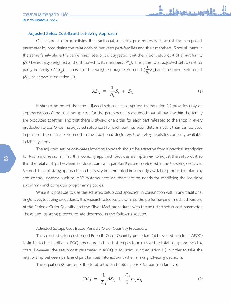
Adjusted Setup Cost-Based Lot-sizing Approach

One approach for modifying the traditional lot-sizing procedures is to adjust the setup cost

parameter by considering the relationships between part-families and their members. Since all parts in

the same family share the same major setup, it is suggested that the major setup cost of a part family

(Si ) be equally weighted and distributed to its members (Ni ). Then, the total adjusted setup cost for

part j in family i (ASij ) is consist of the weighted major setup cost

8

ASij = adjusted setup cost of part j in part-family i;

hij = inventory holding cost per unit per period of part j in part-family i;

TCij = the sum of total annual setup and holding costs of all parts j in part-family i;

dij = the average demand rate per period of part j in part-family i;

dijt = demand of part j in part-family i in period t;

Tij = economic cycle time of part j in part-family i;

Ti = economic cycle time of part-family i; and

xij = 0-1 type variable used for determining whether the minor setup for part j in part-

family i is required in the current production cycle.

PROPOSED LOT-SIZING ALGORITHMS IN FMS

To accomplish this first research objective, two different approaches for modifying

traditional lot-sizing procedures are proposed. In brief, the first approach involves adjusting

the setup cost parameter for each component part by considering the relationships which exist

between component parts and part-families. This adjusted setup cost parameter can then be

used in place of the original setup cost parameter in the traditional single-level lot-sizing

models, such as periodic order quantity, Silver-Meal, and many others. The second approach

involves modifying the algorithms of traditional single-level lot-sizing procedures so that lot-

sizing decisions for the component parts can be made by part-families rather than by

individual parts. In this research, the first lot-sizing approach is referred to as the “adjusted

setup cost lot-sizing approach” and the second approach as the “family-oriented lot-sizing

approach.”


One approach for modifying the traditional lot-sizing procedures is to adjust the setup

cost parameter by considering the relationships between part-families and their members.

Since all parts in the same family share the same major setup, it is suggested that the major

setup cost of a part family (Si) be equally weighted and distributed to its members (Ni). Then,

the total adjusted setup cost for part j in family i (ASij) is consist of the weighted major setup

cost ( 1𝑁𝑁𝑁𝑁𝑖𝑖𝑖𝑖𝑆𝑆𝑆𝑆𝑖𝑖𝑖𝑖) and the minor setup cost (Sij) as shown in equation (1).

𝐴𝐴𝐴𝐴𝑆𝑆𝑆𝑆𝑖𝑖𝑖𝑖𝑖𝑖𝑖𝑖 = 1𝑁𝑁𝑁𝑁𝑖𝑖𝑖𝑖𝑆𝑆𝑆𝑆𝑖𝑖𝑖𝑖 + 𝑆𝑆𝑆𝑆𝑖𝑖𝑖𝑖𝑖𝑖𝑖𝑖 (1)

and the minor setup cost

(Sij ) as shown in equation (1).

8

ASij = adjusted setup cost of part j in part-family i;

hij = inventory holding cost per unit per period of part j in part-family i;

TCij = the sum of total annual setup and holding costs of all parts j in part-family i;

dij = the average demand rate per period of part j in part-family i;

dijt = demand of part j in part-family i in period t;

Tij = economic cycle time of part j in part-family i;

Ti = economic cycle time of part-family i; and

xij = 0-1 type variable used for determining whether the minor setup for part j in part-

family i is required in the current production cycle.

PROPOSED LOT-SIZING ALGORITHMS IN FMS

To accomplish this first research objective, two different approaches for modifying

traditional lot-sizing procedures are proposed. In brief, the first approach involves adjusting

the setup cost parameter for each component part by considering the relationships which exist

between component parts and part-families. This adjusted setup cost parameter can then be

used in place of the original setup cost parameter in the traditional single-level lot-sizing

models, such as periodic order quantity, Silver-Meal, and many others. The second approach

involves modifying the algorithms of traditional single-level lot-sizing procedures so that lot-

sizing decisions for the component parts can be made by part-families rather than by

individual parts. In this research, the first lot-sizing approach is referred to as the “adjusted

setup cost lot-sizing approach” and the second approach as the “family-oriented lot-sizing

approach.”


One approach for modifying the traditional lot-sizing procedures is to adjust the setup

cost parameter by considering the relationships between part-families and their members.

Since all parts in the same family share the same major setup, it is suggested that the major

setup cost of a part family (Si) be equally weighted and distributed to its members (Ni). Then,

the total adjusted setup cost for part j in family i (ASij) is consist of the weighted major setup

cost ( 1𝑁𝑁𝑁𝑁𝑖𝑖𝑖𝑖𝑆𝑆𝑆𝑆𝑖𝑖𝑖𝑖) and the minor setup cost (Sij) as shown in equation (1).

𝐴𝐴𝐴𝐴𝑆𝑆𝑆𝑆𝑖𝑖𝑖𝑖𝑖𝑖𝑖𝑖 = 1𝑁𝑁𝑁𝑁𝑖𝑖𝑖𝑖𝑆𝑆𝑆𝑆𝑖𝑖𝑖𝑖 + 𝑆𝑆𝑆𝑆𝑖𝑖𝑖𝑖𝑖𝑖𝑖𝑖 (1)

It should be noted that the adjusted setup cost computed by equation (1) provides only an

approximation of the total setup cost for the part since it is assumed that all parts within the family

are produced together, and that there is always one order for each part released to the shop in every

production cycle. Once the adjusted setup cost for each part has been determined, it then can be used

in place of the original setup cost in the traditional single-level lot-sizing heuristics currently available

in MRP systems.

The adjusted setups cost-bases lot-sizing approach should be attractive from a practical standpoint

for two major reasons. First, this lot-sizing approach provides a simple way to adjust the setup cost so

that the relationships between individual parts and part-families are considered in the lot-sizing decisions.

Second, this lot-sizing approach can be easily implemented in currently available production planning

and control systems such as MRP systems because there are no needs for modifying the lot-sizing

algorithms and computer programming codes.

While it is possible to use the adjusted setup cost approach in conjunction with many traditional

single-level lot-sizing procedures, this research selectively examines the performance of modified versions

of the Periodic Order Quantity and the Silver-Meal procedures with the adjusted setup cost parameter.

These two lot-sizing procedures are described in the following section.

Adjusted Setups Cost-Based Periodic Order Quantity Procedure

The adjusted setup cost-based Periodic Order Quantity procedure (abbreviated herein as APOQ)

is similar to the traditional POQ procedure in that it attempts to minimize the total setup and holding

costs. However, the setup cost parameter in APOQ is adjusted using equation (1) in order to take the

relationship between parts and part families into account when making lot-sizing decisions.

The equation (2) presents the total setup and holding costs for part j in family i.

9

It should be noted that the adjusted setup cost computed by equation (1) provides only

an approximation of the total setup cost for the part since it is assumed that all parts within

the family are produced together, and that there is always one order for each part released to

the shop in every production cycle. Once the adjusted setup cost for each part has been

determined, it then can be used in place of the original setup cost in the traditional single-

level lot-sizing heuristics currently available in MRP systems.

The adjusted setups cost-bases lot-sizing approach should be attractive from a

practical standpoint for two major reasons. First, this lot-sizing approach provides a simple

way to adjust the setup cost so that the relationships between individual parts and part-

families are considered in the lot-sizing decisions. Second, this lot-sizing approach can be

easily implemented in currently available production planning and control systems such as

MRP systems because there are no needs for modifying the lot-sizing algorithms and

computer programming codes.

While it is possible to use the adjusted setup cost approach in conjunction with many

traditional single-level lot-sizing procedures, this research selectively examines the

performance of modified versions of the Periodic Order Quantity and the Silver-Meal

procedures with the adjusted setup cost parameter. These two lot-sizing procedures are

described in the following section.

Adjusted Setups Cost-Based Periodic Order Quantity Procedure

The adjusted setup cost-based Periodic Order Quantity procedure (abbreviated herein

as APOQ) is similar to the traditional POQ procedure in that it attempts to minimize the total

setup and holding costs. However, the setup cost parameter in APOQ is adjusted using

equation (1) in order to take the relationship between parts and part families into account

when making lot-sizing decisions.

The equation (2) presents the total setup and holding costs for part j in family i.

𝑇𝑇𝑇𝑇𝑇𝑇𝑇𝑇𝑖𝑖𝑖𝑖𝑖𝑖𝑖𝑖 = 1𝑇𝑇𝑇𝑇𝑖𝑖𝑖𝑖𝑖𝑖𝑖𝑖

𝐴𝐴𝐴𝐴𝑆𝑆𝑆𝑆𝑖𝑖𝑖𝑖𝑖𝑖𝑖𝑖 + 𝑇𝑇𝑇𝑇𝑖𝑖𝑖𝑖𝑖𝑖𝑖𝑖2ℎ𝑖𝑖𝑖𝑖𝑖𝑖𝑖𝑖𝑑𝑑𝑑𝑑𝑖𝑖𝑖𝑖𝑖𝑖𝑖𝑖 (2)

By taking the partial derivatives of TCij with respect to Tij, setting the results equal to

zero, and solving for Tij , the optimal value of Tij is as shown in equation (3).

(1)

(2)

89


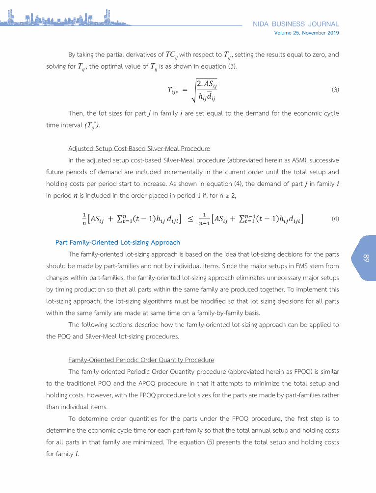
By taking the partial derivatives of TCij with respect to Tij , setting the results equal to zero, and

solving for Tij , the optimal value of Tij is as shown in equation (3).

10

𝑇𝑇𝑇𝑇𝑖𝑖𝑖𝑖𝑖𝑖𝑖𝑖∗ = �2.𝐴𝐴𝐴𝐴𝑆𝑆𝑆𝑆𝑖𝑖𝑖𝑖𝑖𝑖𝑖𝑖ℎ𝑖𝑖𝑖𝑖𝑖𝑖𝑖𝑖𝑑𝑑𝑑𝑑𝑖𝑖𝑖𝑖𝑖𝑖𝑖𝑖

(3)

Then, the lot sizes for part j in family i are set equal to the demand for the economic

cycle time interval (Tij*).

Adjusted Setup Cost-Based Silver-Meal Procedure

In the adjusted setup cost-based Silver-Meal procedure (abbreviated herein as ASM),

successive future periods of demand are included incrementally in the current order until the

total setup and holding costs per period start to increase. As shown in equation (4), the

demand of part j in family i in period n is included in the order placed in period 1 if, for n ≥ 2,

1𝑛𝑛𝑛𝑛�𝐴𝐴𝐴𝐴𝑆𝑆𝑆𝑆𝑖𝑖𝑖𝑖𝑖𝑖𝑖𝑖 + ∑ (𝑡𝑡𝑡𝑡 − 1)ℎ𝑖𝑖𝑖𝑖𝑖𝑖𝑖𝑖𝑛𝑛𝑛𝑛

𝑡𝑡𝑡𝑡=1 𝑑𝑑𝑑𝑑𝑖𝑖𝑖𝑖𝑖𝑖𝑖𝑖𝑡𝑡𝑡𝑡� ≤ 1𝑛𝑛𝑛𝑛−1

�𝐴𝐴𝐴𝐴𝑆𝑆𝑆𝑆𝑖𝑖𝑖𝑖𝑖𝑖𝑖𝑖 + ∑ (𝑡𝑡𝑡𝑡 − 1)ℎ𝑖𝑖𝑖𝑖𝑖𝑖𝑖𝑖𝑑𝑑𝑑𝑑𝑖𝑖𝑖𝑖𝑖𝑖𝑖𝑖𝑡𝑡𝑡𝑡�𝑛𝑛𝑛𝑛−1𝑡𝑡𝑡𝑡=1 (4)

Part Family-Oriented Lot-sizing Approach

The family-oriented lot-sizing approach is based on the idea that lot-sizing decisions

for the parts should be made by part-families and not by individual items. Since the major

setups in FMS stem from changes within part-families, the family-oriented lot-sizing

approach eliminates unnecessary major setups by timing production so that all parts within

the same family are produced together. To implement this lot-sizing approach, the lot-sizing

algorithms must be modified so that lot sizing decisions for all parts within the same family

are made at same time on a family-by-family basis.

The following sections describe how the family-oriented lot-sizing approach can be

applied to the POQ and Silver-Meal lot-sizing procedures.

Family-Oriented Periodic Order Quantity Procedure

The family-oriented Periodic Order Quantity procedure (abbreviated herein as FPOQ)

is similar to the traditional POQ and the APOQ procedure in that it attempts to minimize the

total setup and holding costs. However, with the FPOQ procedure lot sizes for the parts are

made by part-families rather than individual items.

To determine order quantities for the parts under the FPOQ procedure, the first step is

to determine the economic cycle time for each part-family so that the total annual setup and

Then, the lot sizes for part j in family i are set equal to the demand for the economic cycle

time interval (Tij*).


In the adjusted setup cost-based Silver-Meal procedure (abbreviated herein as ASM), successive

future periods of demand are included incrementally in the current order until the total setup and

holding costs per period start to increase. As shown in equation (4), the demand of part j in family i in period n is included in the order placed in period 1 if, for n ≥ 2,

10

𝑇𝑇𝑇𝑇𝑖𝑖𝑖𝑖𝑖𝑖𝑖𝑖∗ = �2.𝐴𝐴𝐴𝐴𝑆𝑆𝑆𝑆𝑖𝑖𝑖𝑖𝑖𝑖𝑖𝑖ℎ𝑖𝑖𝑖𝑖𝑖𝑖𝑖𝑖𝑑𝑑𝑑𝑑𝑖𝑖𝑖𝑖𝑖𝑖𝑖𝑖

(3)

Then, the lot sizes for part j in family i are set equal to the demand for the economic

cycle time interval (Tij*).


In the adjusted setup cost-based Silver-Meal procedure (abbreviated herein as ASM),

successive future periods of demand are included incrementally in the current order until the

total setup and holding costs per period start to increase. As shown in equation (4), the

demand of part j in family i in period n is included in the order placed in period 1 if, for n ≥ 2,

1𝑛𝑛𝑛𝑛�𝐴𝐴𝐴𝐴𝑆𝑆𝑆𝑆𝑖𝑖𝑖𝑖𝑖𝑖𝑖𝑖 + ∑ (𝑡𝑡𝑡𝑡 − 1)ℎ𝑖𝑖𝑖𝑖𝑖𝑖𝑖𝑖𝑛𝑛𝑛𝑛

𝑡𝑡𝑡𝑡=1 𝑑𝑑𝑑𝑑𝑖𝑖𝑖𝑖𝑖𝑖𝑖𝑖𝑡𝑡𝑡𝑡� ≤ 1𝑛𝑛𝑛𝑛−1

�𝐴𝐴𝐴𝐴𝑆𝑆𝑆𝑆𝑖𝑖𝑖𝑖𝑖𝑖𝑖𝑖 + ∑ (𝑡𝑡𝑡𝑡 − 1)ℎ𝑖𝑖𝑖𝑖𝑖𝑖𝑖𝑖𝑑𝑑𝑑𝑑𝑖𝑖𝑖𝑖𝑖𝑖𝑖𝑖𝑡𝑡𝑡𝑡�𝑛𝑛𝑛𝑛−1𝑡𝑡𝑡𝑡=1 (4)


The family-oriented lot-sizing approach is based on the idea that lot-sizing decisions

for the parts should be made by part-families and not by individual items. Since the major

setups in FMS stem from changes within part-families, the family-oriented lot-sizing

approach eliminates unnecessary major setups by timing production so that all parts within

the same family are produced together. To implement this lot-sizing approach, the lot-sizing

algorithms must be modified so that lot sizing decisions for all parts within the same family

are made at same time on a family-by-family basis.

The following sections describe how the family-oriented lot-sizing approach can be

applied to the POQ and Silver-Meal lot-sizing procedures.


The family-oriented Periodic Order Quantity procedure (abbreviated herein as FPOQ)

is similar to the traditional POQ and the APOQ procedure in that it attempts to minimize the

total setup and holding costs. However, with the FPOQ procedure lot sizes for the parts are

made by part-families rather than individual items.

To determine order quantities for the parts under the FPOQ procedure, the first step is

to determine the economic cycle time for each part-family so that the total annual setup and


The family-oriented lot-sizing approach is based on the idea that lot-sizing decisions for the parts

should be made by part-families and not by individual items. Since the major setups in FMS stem from

changes within part-families, the family-oriented lot-sizing approach eliminates unnecessary major setups

by timing production so that all parts within the same family are produced together. To implement this

lot-sizing approach, the lot-sizing algorithms must be modified so that lot sizing decisions for all parts

within the same family are made at same time on a family-by-family basis.

The following sections describe how the family-oriented lot-sizing approach can be applied to

the POQ and Silver-Meal lot-sizing procedures.


The family-oriented Periodic Order Quantity procedure (abbreviated herein as FPOQ) is similar

to the traditional POQ and the APOQ procedure in that it attempts to minimize the total setup and

holding costs. However, with the FPOQ procedure lot sizes for the parts are made by part-families rather

than individual items.

To determine order quantities for the parts under the FPOQ procedure, the first step is to

determine the economic cycle time for each part-family so that the total annual setup and holding costs

for all parts in that family are minimized. The equation (5) presents the total setup and holding costs

for family i.

(4)

(3)

90


(5)

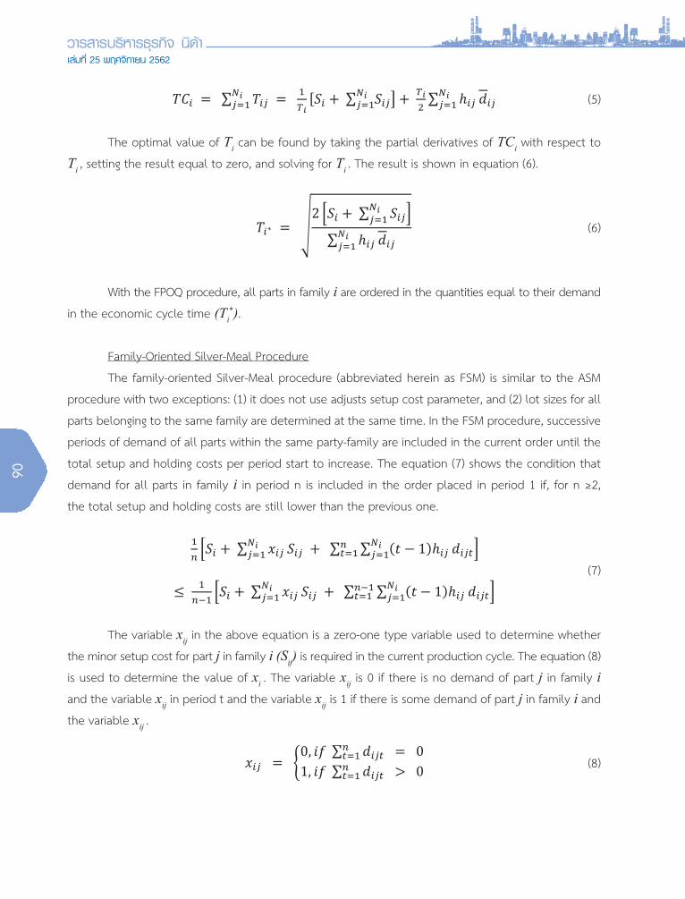
The optimal value of Ti can be found by taking the partial derivatives of TCi with respect to

Ti , setting the result equal to zero, and solving for Ti . The result is shown in equation (6).

11

holding costs for all parts in that family are minimized. The equation (5) presents the total

setup and holding costs for family i.

𝑇𝑇𝑇𝑇𝑇𝑇𝑇𝑇𝑖𝑖𝑖𝑖 = ∑ 𝑇𝑇𝑇𝑇𝑖𝑖𝑖𝑖𝑖𝑖𝑖𝑖𝑁𝑁𝑁𝑁𝑖𝑖𝑖𝑖𝑖𝑖𝑖𝑖=1 = 1

𝑇𝑇𝑇𝑇𝑖𝑖𝑖𝑖[𝑆𝑆𝑆𝑆𝑖𝑖𝑖𝑖 + ∑ 𝑆𝑆𝑆𝑆𝑖𝑖𝑖𝑖𝑖𝑖𝑖𝑖�

𝑁𝑁𝑁𝑁𝑖𝑖𝑖𝑖𝑖𝑖𝑖𝑖=1 + 𝑇𝑇𝑇𝑇𝑖𝑖𝑖𝑖

2∑ ℎ𝑖𝑖𝑖𝑖𝑖𝑖𝑖𝑖𝑁𝑁𝑁𝑁𝑖𝑖𝑖𝑖𝑖𝑖𝑖𝑖=1 𝑑𝑑𝑑𝑑𝑖𝑖𝑖𝑖𝑖𝑖𝑖𝑖 (5)

The optimal value of Ti can be found by taking the partial derivatives of TCi with

respect to Ti, setting the result equal to zero, and solving for Ti. The result is shown in

equation (6).

𝑇𝑇𝑇𝑇𝑖𝑖𝑖𝑖∗ = �2 �𝑆𝑆𝑆𝑆𝑖𝑖𝑖𝑖 + ∑ 𝑆𝑆𝑆𝑆𝑖𝑖𝑖𝑖𝑖𝑖𝑖𝑖

𝑁𝑁𝑁𝑁𝑖𝑖𝑖𝑖𝑖𝑖𝑖𝑖=1 �

∑ ℎ𝑖𝑖𝑖𝑖𝑖𝑖𝑖𝑖𝑁𝑁𝑁𝑁𝑖𝑖𝑖𝑖𝑖𝑖𝑖𝑖=1 𝑑𝑑𝑑𝑑𝑖𝑖𝑖𝑖𝑖𝑖𝑖𝑖

(6)

With the FPOQ procedure, all parts in family i are ordered in the quantities equal to

their demand in the economic cycle time (Ti*).

Family-Oriented Silver-Meal Procedure

The family-oriented Silver-Meal procedure (abbreviated herein as FSM) is similar to

the ASM procedure with two exceptions: (1) it does not use adjusts setup cost parameter, and

(2) lot sizes for all parts belonging to the same family are determined at the same time. In the

FSM procedure, successive periods of demand of all parts within the same party-family are

included in the current order until the total setup and holding costs per period start to

increase. The equation (7) shows the condition that demand for all parts in family i in period

n is included in the order placed in period 1 if, for n ≥2, the total setup and holding costs are

still lower than the previous one.

1𝑛𝑛𝑛𝑛�𝑆𝑆𝑆𝑆𝑖𝑖𝑖𝑖 + ∑ 𝑥𝑥𝑥𝑥𝑖𝑖𝑖𝑖𝑖𝑖𝑖𝑖

𝑁𝑁𝑁𝑁𝑖𝑖𝑖𝑖𝑖𝑖𝑖𝑖=1 𝑆𝑆𝑆𝑆𝑖𝑖𝑖𝑖𝑖𝑖𝑖𝑖 + ∑ ∑ (𝑡𝑡𝑡𝑡 − 1)ℎ𝑖𝑖𝑖𝑖𝑖𝑖𝑖𝑖

𝑁𝑁𝑁𝑁𝑖𝑖𝑖𝑖𝑖𝑖𝑖𝑖=1

𝑛𝑛𝑛𝑛𝑡𝑡𝑡𝑡=1 𝑑𝑑𝑑𝑑𝑖𝑖𝑖𝑖𝑖𝑖𝑖𝑖𝑡𝑡𝑡𝑡�

≤ 1𝑛𝑛𝑛𝑛−1

�𝑆𝑆𝑆𝑆𝑖𝑖𝑖𝑖 + ∑ 𝑥𝑥𝑥𝑥𝑖𝑖𝑖𝑖𝑖𝑖𝑖𝑖𝑁𝑁𝑁𝑁𝑖𝑖𝑖𝑖𝑖𝑖𝑖𝑖=1 𝑆𝑆𝑆𝑆𝑖𝑖𝑖𝑖𝑖𝑖𝑖𝑖 + ∑ ∑ (𝑡𝑡𝑡𝑡 − 1)ℎ𝑖𝑖𝑖𝑖𝑖𝑖𝑖𝑖


𝑛𝑛𝑛𝑛−1𝑡𝑡𝑡𝑡=1 𝑑𝑑𝑑𝑑𝑖𝑖𝑖𝑖𝑖𝑖𝑖𝑖𝑡𝑡𝑡𝑡� (7)

The variable xij in the above equation is a zero-one type variable used to determine

whether the minor setup cost for part j in family i (Sij) is required in the current production

cycle. The equation (8) is used to determine the value of xi. The variable xij is 0 if there is no

demand of part j in family i and the variable xij in period t and the variable xij is 1 if there is

some demand of part j in family i and the variable xij.

With the FPOQ procedure, all parts in family i are ordered in the quantities equal to their demand

in the economic cycle time (Ti*).


The family-oriented Silver-Meal procedure (abbreviated herein as FSM) is similar to the ASM

procedure with two exceptions: (1) it does not use adjusts setup cost parameter, and (2) lot sizes for all

parts belonging to the same family are determined at the same time. In the FSM procedure, successive

periods of demand of all parts within the same party-family are included in the current order until the

total setup and holding costs per period start to increase. The equation (7) shows the condition that

demand for all parts in family i in period n is included in the order placed in period 1 if, for n ≥2,

the total setup and holding costs are still lower than the previous one.

11









equation (6).




(6)

























11









equation (6).




(6)

























The variable xij in the above equation is a zero-one type variable used to determine whether

the minor setup cost for part j in family i (Sij) is required in the current production cycle. The equation (8)

is used to determine the value of xi . The variable xij is 0 if there is no demand of part j in family i and the variable xij in period t and the variable xij is 1 if there is some demand of part j in family i and

the variable xij .

12

𝑥𝑥𝑥𝑥𝑖𝑖𝑖𝑖𝑖𝑖𝑖𝑖 = �0, 𝑖𝑖𝑖𝑖𝑖𝑖𝑖𝑖 ∑ 𝑑𝑑𝑑𝑑𝑖𝑖𝑖𝑖𝑖𝑖𝑖𝑖𝑡𝑡𝑡𝑡𝑛𝑛𝑛𝑛

𝑡𝑡𝑡𝑡=1 = 01, 𝑖𝑖𝑖𝑖𝑖𝑖𝑖𝑖 ∑ 𝑑𝑑𝑑𝑑𝑖𝑖𝑖𝑖𝑖𝑖𝑖𝑖𝑡𝑡𝑡𝑡𝑛𝑛𝑛𝑛

𝑡𝑡𝑡𝑡=1 > 0 (8)

RESEARCH METHODOLOGY

This research uses the simulation method to investigate the performance of five

different lot-sizing algorithms in a hypothetical FMS under different operating conditions.

The five lot-sizing procedures tested in the experiments include: (1) adjusted order quantity

with setup cost procedure, (2) adjusted Silver-Meal with setup cost procedure, (3) family-

oriented periodic order quantity procedure, (4) family-oriented Silver-Meal procedure, and

(5) lot-for-lot procedure. The experimental design used in this research is a 5 x 26 full

factorial repeated measures design with seven independent variables as follows.

Independent Variables Level Description 1. Lot-sizing procedure (LS) 1 APOQ (Adjusted periodic order quantity with setup cost)

2 ASM (adjusted Silver-Meal with setup cost)

3 FPOQ (family-oriented periodic order quantity)

4 FSM (family-oriented Silver-Meal)

5 LFL (Loy-for-Lot)

2.End-product demand variability(DV) 1 Low: constant at 50

2

High: uniform distribution with a mean of 50 and a range of ±50

3.End-product demand uncertainty(DU) 1

Low: normal distribution with a mean of 0 and a standard deviation of 15

2

High: normal distribution with a mean of 0 and a standard deviation of 30

4.Number of parts per family (NP) 1 Low: 2 parts/family

2 High: 4 parts/family

5.Major to minor setup times ratio(SR) 1 Low: 2:1

2 High: 6:1

6.Setup to holding cost rate ratio (CR) 1 Low: 100:1

2 High: 200:1

7.Capacity utilization (UT) 1 Low: 65%

2 High: 85%

(6)

(7)

(8)

11









equation (6).




(6)

























91


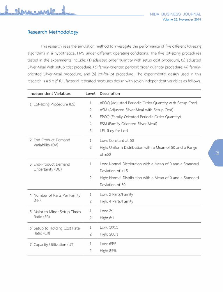
Research Methodology

This research uses the simulation method to investigate the performance of five different lot-sizing

algorithms in a hypothetical FMS under different operating conditions. The five lot-sizing procedures

tested in the experiments include: (1) adjusted order quantity with setup cost procedure, (2) adjusted

Silver-Meal with setup cost procedure, (3) family-oriented periodic order quantity procedure, (4) family-

oriented Silver-Meal procedure, and (5) lot-for-lot procedure. The experimental design used in this

research is a 5 x 26 full factorial repeated measures design with seven independent variables as follows.

Independent Variables Level Description

1. Lot-sizing Procedure (LS) 1

2

3

4

5

APOQ (Adjusted Periodic Order Quantity with Setup Cost)

ASM (Adjusted Silver-Meal with Setup Cost)

FPOQ (Family-Oriented Periodic Order Quantity)

FSM (Family-Oriented Silver-Meal)

LFL (Loy-for-Lot)

2. End-Product Demand Variability (DV)

1

2

Low: Constant at 50

High: Uniform Distribution with a Mean of 50 and a Range

of ±50

3. End-Product Demand Uncertainty (DU)

1

2

Low: Normal Distribution with a Mean of 0 and a Standard

Deviation of ±15

High: Normal Distribution with a Mean of 0 and a Standard

Deviation of 30

4. Number of Parts Per Family (NP)

1

2

Low: 2 Parts/Family

High: 4 Parts/Family

5. Major to Minor Setup Times Ratio (SR)

1

2

Low: 2:1

High: 6:1

6. Setup to Holding Cost Rate Ratio (CR)

1

2

Low: 100:1

High: 200:1

7. Capacity Utilization (UT) 1

2

Low: 65%

High: 85%

92


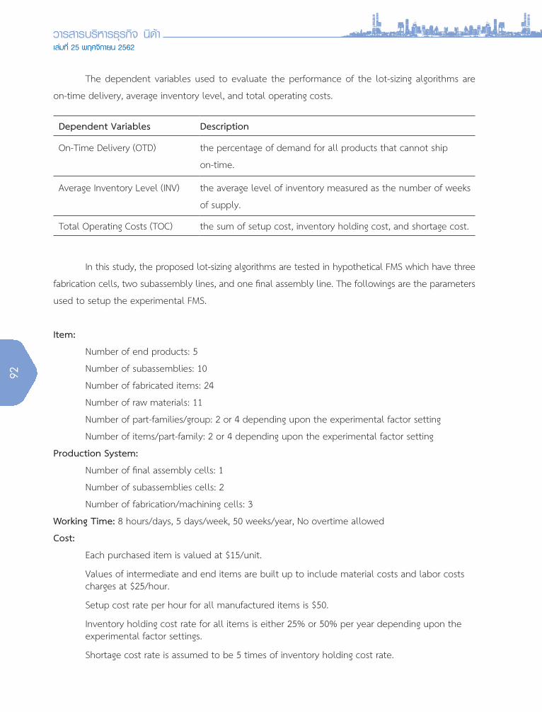
Dependent Variables Description

On-Time Delivery (OTD) the percentage of demand for all products that cannot ship

on-time.

Average Inventory Level (INV) the average level of inventory measured as the number of weeks

of supply.

Total Operating Costs (TOC) the sum of setup cost, inventory holding cost, and shortage cost.

In this study, the proposed lot-sizing algorithms are tested in hypothetical FMS which have three

fabrication cells, two subassembly lines, and one final assembly line. The followings are the parameters

used to setup the experimental FMS.

Item:

Number of end products: 5

Number of subassemblies: 10

Number of fabricated items: 24

Number of raw materials: 11

Number of part-families/group: 2 or 4 depending upon the experimental factor setting

Number of items/part-family: 2 or 4 depending upon the experimental factor setting

Production System:

Number of final assembly cells: 1

Number of subassemblies cells: 2

Number of fabrication/machining cells: 3

Working Time: 8 hours/days, 5 days/week, 50 weeks/year, No overtime allowed

Cost:

Each purchased item is valued at $15/unit.

Values of intermediate and end items are built up to include material costs and labor costs charges at $25/hour.

Setup cost rate per hour for all manufactured items is $50.

Inventory holding cost rate for all items is either 25% or 50% per year depending upon the experimental factor settings.

Shortage cost rate is assumed to be 5 times of inventory holding cost rate.

The dependent variables used to evaluate the performance of the lot-sizing algorithms are

on-time delivery, average inventory level, and total operating costs.

93


Lead Time:

For end products: 1 week

For subassemblies: 1 week

For fabricated items: 4 weeks

For raw materials: assumed instantaneously delivery

Planning Horizon: 24 weeks; this is four times of cumulative lead times of end products

Dispatching Rule: Earliest due date

Data Collection Method

In this research, data are collected using the “batch means” approach (Fishman, 1978; Law &

Kelton, 1982) in which, for each cell in the experiments, one long simulation run is performed, and

that run is broken down into “batches” or “sub-runs”. To eliminate the effect of transient conditions,

the experimental production systems are initially operated for 300 weeks and the performance measures

are then re-initialized. The systems will continue to operate thereafter for 200 weeks. At the end of

every 50 weeks, the required statistics are recorded, and the performance measures are again initialized.

A common set of random collection method, there is a total of 4x 5x 26 or 1280.

Data Analysis Methods

A series of Analysis of variance (ANOVA) is used to analyze the data to examine the interaction

effects between the lot-sizing algorithms and the operating environmental factors and Duncan’s multiple

range test is used to examine the relative performance of lot-sizing algorithms.

Research Questions

The following research questions are to be addressed in this research:

(1) Are the performance measures significantly related to the lot-sizing algorithms used?

(2) Is there one lot-sizing algorithm that always outperforms the others in all operating

environment settings? If so, which lot-sizing algorithm is superior?

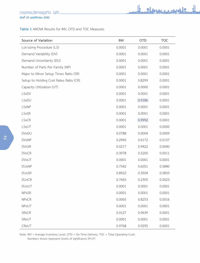
Data Analysis and Results

To examine interaction effects between the lot-sizing algorithms and the operating environmental

factors (i.e., DV, DU, NP, SR, CR and UT), the experimental data is analyzed by the analysis of variance

technique. The results from the analyses are shown in Table 1.

94


Table 1 ANOVA Results for INV, OTD and TOC Measures

Source of Variation INV OTD TOC

Lot-sizing Procedure (LS) 0.0001 0.0001 0.0001

Demand Variability (DV) 0.0001 0.0001 0.0001

Demand Uncertainty (DU) 0.0001 0.0001 0.0001

Number of Parts Per Family (NP) 0.0001 0.0001 0.0001

Major to Minor Setup Times Ratio (SR) 0.0001 0.0001 0.0001

Setup to Holding Cost Rates Ratio (CR) 0.0001 0.8299 0.0001

Capacity Utilization (UT) 0.0001 0.0000 0.0001

LSxDV 0.0001 0.0001 0.0001

LSxDU 0.0001 0.9186 0.0001

LSxNP 0.0001 0.0001 0.0001

LSxSR 0.0001 0.0001 0.0001

LSxCR 0.0001 0.9992 0.0001

LSxUT 0.0001 0.0001 0.0000

DVxDU 0.0788 0.0004 0.0009

DVxNP 0.2943 0.6172 0.0137

DVxSR 0.0217 0.9422 0.0040

DVxCR 0.3978 0.5200 0.0011

DVxUT 0.0001 0.0001 0.0001

DUxNP 0.7542 0.6051 0.5840

DUxSR 0.8922 0.3504 0.5833

DUxCR 0.7665 0.2305 0.0023

DUxUT 0.0001 0.0001 0.0001

NPxSR 0.0001 0.0001 0.0001

NPxCR 0.0065 0.8253 0.0016

NPxUT 0.0001 0.0001 0.0001

SRxCR 0.0127 0.9639 0.0001

SRxUT 0.0001 0.0001 0.0001

CRxUT 0.9768 0.9295 0.0001

Note: INV = Average Inventory Level, OTD = On-Time Delivery, TOC = Total Operating Costs Numbers shows represent levels of significance (Pr>F)

95


An examination of the levels of significance presented in Table 1 reveals that the lot-sizing

algorithm main effect is significant for every one of the INV, OTD and TOC measures at the 0.05 level of

significance. For the interaction effects between the lot-sizing algorithms and the operating environmental

factors, the results indicate that the interactions between the lot-sizing algorithms and almost all

operating environmental factors are significant for every one of the INV, OTD and TOC measures at the

0.05 level of significance, except the interaction effects between the lot-sizing algorithms and the end-

product demand uncertainty (LSxDU), and between the lot-sizing algorithms and the setup to holding

cost rates ratio (LSxCR) are insignificant for the OTD measure, but significant for the INV and TOC

measures at the 0.05 level.

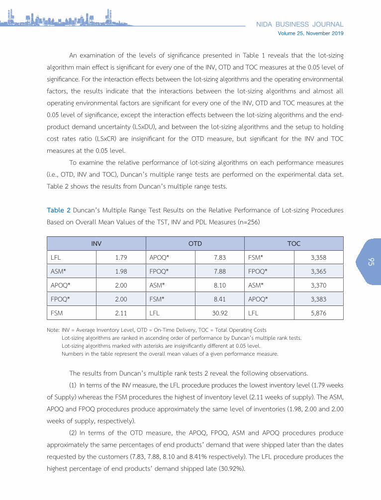
To examine the relative performance of lot-sizing algorithms on each performance measures

(i.e., OTD, INV and TOC), Duncan’s multiple range tests are performed on the experimental data set.

Table 2 shows the results from Duncan’s multiple range tests.

Table 2 Duncan’s Multiple Range Test Results on the Relative Performance of Lot-sizing Procedures

Based on Overall Mean Values of the TST, INV and PDL Measures (n=256)

INV OTD TOC

LFL 1.79 APOQ* 7.83 FSM* 3,358

ASM* 1.98 FPOQ* 7.88 FPOQ* 3,365

APOQ* 2.00 ASM* 8.10 ASM* 3,370

FPOQ* 2.00 FSM* 8.41 APOQ* 3,383

FSM 2.11 LFL 30.92 LFL 5,876

Note: INV = Average Inventory Level, OTD = On-Time Delivery, TOC = Total Operating Costs Lot-sizing algorithms are ranked in ascending order of performance by Duncan’s multiple rank tests. Lot-sizing algorithms marked with asterisks are insignificantly different at 0.05 level. Numbers in the table represent the overall mean values of a given performance measure.

The results from Duncan’s multiple rank tests 2 reveal the following observations.

(1) In terms of the INV measure, the LFL procedure produces the lowest inventory level (1.79 weeks

of Supply) whereas the FSM procedures the highest of inventory level (2.11 weeks of supply). The ASM,

APOQ and FPOQ procedures produce approximately the same level of inventories (1.98, 2.00 and 2.00

weeks of supply, respectively).

(2) In terms of the OTD measure, the APOQ, FPOQ, ASM and APOQ procedures produce

approximately the same percentages of end products’ demand that were shipped later than the dates

requested by the customers (7.83, 7.88, 8.10 and 8.41% respectively). The LFL procedure produces the

highest percentage of end products’ demand shipped late (30.92%).

96


(3) In terms of the TOC measures, the FSM, APOQ, FPOQ, ASM and FSM procedures produce

approximately the same total operating costs ($3,358, $3,365, $3,370 and $3,383 respectively). The LFL

procedure produces the highest total costs ($5,876).

Conclusions

In the first part of this research, two different approaches (i.e., adjusted setup cost-oriented and

family-oriented lot-sizing approaches) for modifying the traditional periodic order quantity and Silver-

Meal procedures have been proposed. The first approach involves adjusting the setup cost parameter

for each component part in order to take the part-family relationships into account when determining

lot-sizes for the parts. The equation for adjusting the setup cost parameter has been provided.

This adjusted setup cost parameter is, then, used in place of the original setup cost parameter in the

traditional periodic order quantity and Silver-Meal procedures. The second approach involves modifying

the algorithms of the traditional periodic order quantity and Silver-Meal procedures so that lot-sizing

decisions for the parts can be made by part-families rather by individual parts.

In the second part of this research, a series of simulation experiments was conducted to examine

the performance of five selected lot-sizing algorithms in a hypothetical FMS which has three fabrication

cells, two subassembly lines, and one final assembly line. There are seven independent variables in

the experiments. The first independent variable represents the lot-sizing procedures tested, including

adjusted setup cost-oriented periodic order quantity (APOQ), adjusted setup cost-oriented Silver-Meal

(ASM), family-oriented periodic order quantity (FPOQ), family-oriented Silver-Meal (FSM), and a lot-for-lot

(LFL). The remaining independent variables represent the variables which define the operating conditions

of the FMS, including end-product demand variability, end-product demand uncertainty, number of parts

per family, major to minor setup times ratio, setup to holding cost rates ratio, and capacity utilization.

The tested lot-sizing algorithms were evaluated by three measures (i.e., dependent variables), including

on-time delivery (OTD), average inventory level (INV), and total operating costs (TOC).

The major findings from the experiments may be summarized as follows.

(1) The performance of FMS is significantly affected by the types of lot-sizing algorithms used.

(2) No particular lot-sizing algorithm performs the best in all performance measures in all shop

operating conditions simultaneously.

(3) There is no one best lot-sizing algorithm that is always dominant to the others in all shop

operating conditions.

(4) The lot-for-lot (LFL) can achieve the lowest inventory level (INV) but performs significantly

worse than the other lot-sizing algorithms in terms of on-time delivery (OTD) and total operating costs

(TOC).

97


(5) The adjusted setup cost-oriented periodic order quantity (APOQ), adjusted setup cost-oriented

Silver-Meal (ASM), family-oriented periodic order quantity (FPOQ), and family-oriented Silver-Meal (FSM)

algorithms perform equally well in terms of on-time delivery and total operating costs.

From the practitioners’ point of view, this research demonstrates that the adjusted setup costs

approach and the part-family oriented approach may be used to modify the traditional lot-sizing

algorithms currently available in their computerized MRP systems. These modifications are simple and

minimal. Some industries should benefit from this research such as automobile, electronics and home

appliance.

From the academicians’ point of view, this research has provided the foundations for further

research in solving the lot-sizing problems in FMS. Some examples of such research directions are:

(1) In this research the adjusted setup cost-based and family-oriented lot-sizing approaches

were applied to the periodic order quantity and Silver-Meal lot-sizing procedures. However, these two

lot-sizing approaches may also be applied to other traditional lot-sizing procedures as well. Therefore,

it is logical to extend this research to include other lot-sizing procedures (e.g., part-period balancing,

Groff’s, and least unit cost procedures).

(2) In this research, the adjusted setup cost equation used in the adjusted setup cost-based

lot-sizing approach was derived under an assumption that the probability that all parts are produced

together in a single order cycle is 100%. However, it is possible that all parts may not be processed

together in a single ordering cycle. Therefore, another future research direction may be to develop

different ways to derive adjusted setup cost parameters.

(3) The lot-sizing procedures proposed in this research do not consider capacity limitations when

determining lot sizes for the parts. Therefore, another future research direction is to develop and test

capacitated lot-sizing procedures.

(4) In this research, only one dispatching rule (i.e., earliest due date) was used. However, it is

possible that some other dispatching rules may be used as well. In future research, the performance

of adjusted setup cost-based and family-oriented lot-sizing procedures in conjunction with various

dispatching rules should be examined.

(5) Finally, this research should be extended to examine the performance of the adjusted setup

cost-based and family-oriented lot-sizing procedures in different operating environments (e.g., more

complex product structures and different FMS settings).

98


References

Almada-lobo B., Klabjan D., Carravilla M.A., & Oliveira J., (2007), Single machine multi-product capacitated

lot-sizing with sequencing-dependent setup; International Journal of Production Research, 45;

4873-4894.

Arn, E. (1975), Group technology; Heidelberg: Springer-Verlag.

Burbidge, J. L. (1975), The introduction of group technology; New York: Wiley.

Burbidge, J. L. (1979), Group technology in the engineering industry; London: Mechanical Engineering

Publications Ltd.

Clark A.R., Neto R.M., Toso E.A.V. (2006), Multi-period production setup-sequencing and lo-sizing through

ATSP subtour elimination and pitching; In: Proceedings of the 25th workshop of the UK planning

and scheduling special interest group. University of Nottingham; 80-87.

Devries, M., Harvey, S., & Tipnis, V. (1976), Group technology: An overview and bibliography; Cincinnati,

Ohio: The Machinability Data Center.

Edwards, G. A. B. (1971), Readings in group technology cellular systems; London: The Machinery Publishing

Co., Ltd.

Fogarty, D. W., & Barringer, R. L. (1984), Scheduling manufacturing cells and flexible manufacturing systems;

Proceedings of the Zero Inventory Philosophy and Practices Seminar, 104-110.

Fogarty, D. W., & Barringer, R. L. (1987), Joint order release decisions under dependent demand; Production

and Inventory Management, 28(1), 55-61.

Gallagher, C. C., & Night, W. A. (1973), Group technology; London: Butterworths.

Ham, I., Hitomi, K., & Yoshida, T. (1985), Group technology: Applications to production management;

Boston: Kluwer-Nijhoff Publishing.

Hyer, N. L. (Ed.). (1984a), Group technology at work; Dearborn, Michigan: Society of Manufacturing

Engineers.

Hyer, N. L. (1984b), The potential of group technology for U.S. manufacturing; Journal of Operations

Management, 4(3), 183-202.

Hyer, N. L., & Wemmerlov, U. (1982), MRP/GT: A framework for production planning and control for cellular

manufacturing; Decision Sciences, 13(1), 681-701.

Hyer, N. L., & Wemmerlov, U. (1984), Group technology and productivity; Harvard Business Review, 62,

140-149.

Levulis, T. S. (1978), Group technology–A review of the state of the art in the United States; Chicago,

Illinois: K.W. Tunnell Company.

Mahdieh M., Bijari M., & Clark A. (2011), Simultaneous lot-sizing and scheduling in a flexible flow line;

Journal of Industrial and Systems Engineering, 5(2), 107-119.

99


Mitrofanov, S. P. (1966), Scientific principles of group technology. (English translation), J. Grayson (Ed.);

London: National Lending Library for Science and Technology.

Patterson, W. J., & LaForge, L. R. (1985), The incremental part period algorithm: An alternative to EOQ;

Journal of Purchasing and Materials Management, 21(2), 28-33.

Petrov, V. A. (1966), Flow line group planning. (English translation), E. Morris (Ed.), Yorkshire: National Lending

Co. Petrov, V. A. (1968). Flow line group production planning; London: Business Publications.

Rabbi, M. F., & Lakhamani, G. (1984), Relationship between group technology and material requirements

planning; Proceedings of the 1984 Annual International Industrial Engineering Conference, 483-486.

Ranson, G. (1972), Group technology. London: McGraw-Hill. Suresh, N. C. (1979). Optimizing intermittent

production systems through group technology and an MRP system; Production and Inventory

Management, 20(4), 77-84.

Wemmerlov, U., & Hyer, N. L. (1987), Research issues in cellular manufacturing; International Journal of

Production Research, 25(3), 413-431.

Documents

Lot-sizing Algorithms in Flexible Manufacturing Systems