Embed Size (px)
Citation preview
1
Outline
• Lot Sizing• Lot Sizing Methods
– Lot-for-Lot (L4L)– EOQ– Silver-Meal Heuristic– Least Unit Cost (LUC)– Part Period Balancing
LESSON 22: MATERIAL REQUIREMENTS PLANNING: LOT SIZING
2
Lot-Sizing
• In Lesson 21 – We employ lot for lot ordering policy and order
production as much as it is needed. – Exception are only the cases in which there are
constraints on the order quantity. – For example, in one case we assume that at least 50
units must be ordered. In another case we assume that the order quantity must be a multiple of 50.
• The motivation behind using lot for lot policy is minimizing inventory. If we order as much as it is needed, there will be no ending inventory at all!
3
Lot-Sizing
• However, lot for lot policy requires that an order be placed each period. So, the number of orders and ordering cost are maximum.
• So, if the ordering cost is significant, one may naturally try to combine some lots into one in order to reduce the ordering cost. But then, inventory holding cost increases.
• Therefore, a question is what is the optimal size of the lot? How many periods will be covered by the first order, the second order, and so on until all the periods in the planning horizon are covered. This is the question of lot sizing. The next slide contains the statement of the lot sizing problem.
4
Lot-Sizing
• The lot sizing problem is as follows: Given net requirements of an item over the next T periods, T >0, find order quantities that minimize the total holding and ordering costs over T periods.
• Note that this is a case of deterministic demand. However, the methods learnt in Lessons 11-15 are not appropriate because – the demand is not necessarily the same over all
periods and– the inventory holding cost is only charged on ending
inventory of each period
5
Lot-Sizing
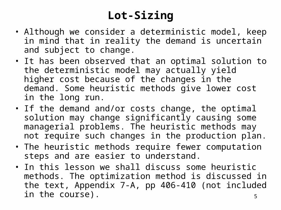
• Although we consider a deterministic model, keep in mind that in reality the demand is uncertain and subject to change.
• It has been observed that an optimal solution to the deterministic model may actually yield higher cost because of the changes in the demand. Some heuristic methods give lower cost in the long run.
• If the demand and/or costs change, the optimal solution may change significantly causing some managerial problems. The heuristic methods may not require such changes in the production plan.
• The heuristic methods require fewer computation steps and are easier to understand.
• In this lesson we shall discuss some heuristic methods. The optimization method is discussed in the text, Appendix 7-A, pp 406-410 (not included in the course).
6
Lot-Sizing
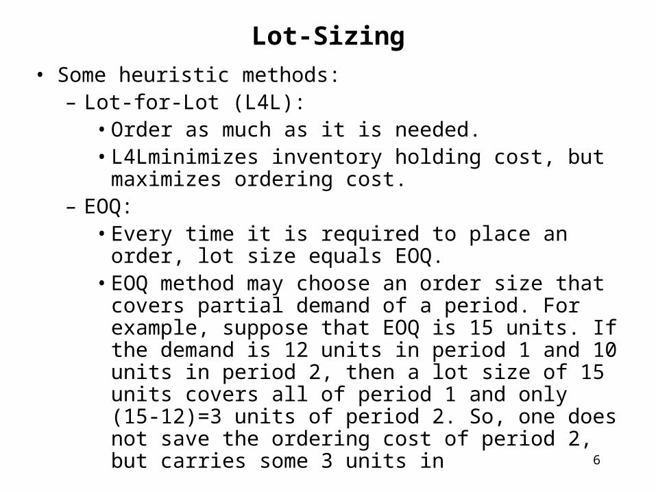
• Some heuristic methods:– Lot-for-Lot (L4L):
• Order as much as it is needed. • L4Lminimizes inventory holding cost, but maximizes
ordering cost.– EOQ:
• Every time it is required to place an order, lot size equals EOQ.
• EOQ method may choose an order size that covers partial demand of a period. For example, suppose that EOQ is 15 units. If the demand is 12 units in period 1 and 10 units in period 2, then a lot size of 15 units covers all of period 1 and only (15-12)=3 units of period 2. So, one does not save the ordering cost of period 2, but carries some 3 units in
7
Lot-Sizing
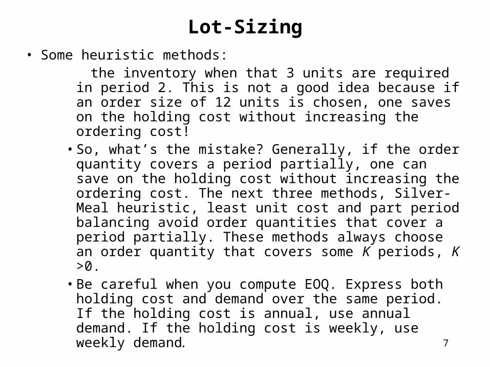
• Some heuristic methods: the inventory when that 3 units are required in
period 2. This is not a good idea because if an order size of 12 units is chosen, one saves on the holding cost without increasing the ordering cost!
• So, what’s the mistake? Generally, if the order quantity covers a period partially, one can save on the holding cost without increasing the ordering cost. The next three methods, Silver-Meal heuristic, least unit cost and part period balancing avoid order quantities that cover a period partially. These methods always choose an order quantity that covers some K periods, K >0.
• Be careful when you compute EOQ. Express both holding cost and demand over the same period. If the holding cost is annual, use annual demand. If the holding cost is weekly, use weekly demand.
8
Lot-Sizing
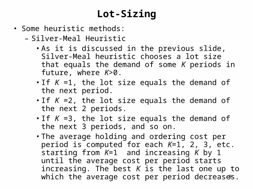
• Some heuristic methods:– Silver-Meal Heuristic
• As it is discussed in the previous slide, Silver-Meal heuristic chooses a lot size that equals the demand of some K periods in future, where K>0.
• If K =1, the lot size equals the demand of the next period.
• If K =2, the lot size equals the demand of the next 2 periods.
• If K =3, the lot size equals the demand of the next 3 periods, and so on.
• The average holding and ordering cost per period is computed for each K=1, 2, 3, etc. starting from K=1 and increasing K by 1 until the average cost per period starts increasing. The best K is the last one up to which the average cost per period decreases.
9
Lot-Sizing
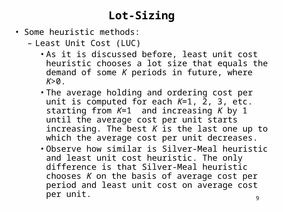
• Some heuristic methods:– Least Unit Cost (LUC)
• As it is discussed before, least unit cost heuristic chooses a lot size that equals the demand of some K periods in future, where K>0.
• The average holding and ordering cost per unit is computed for each K=1, 2, 3, etc. starting from K=1 and increasing K by 1 until the average cost per unit starts increasing. The best K is the last one up to which the average cost per unit decreases.
• Observe how similar is Silver-Meal heuristic and least unit cost heuristic. The only difference is that Silver-Meal heuristic chooses K on the basis of average cost per period and least unit cost on average cost per unit.
10
Lot-Sizing
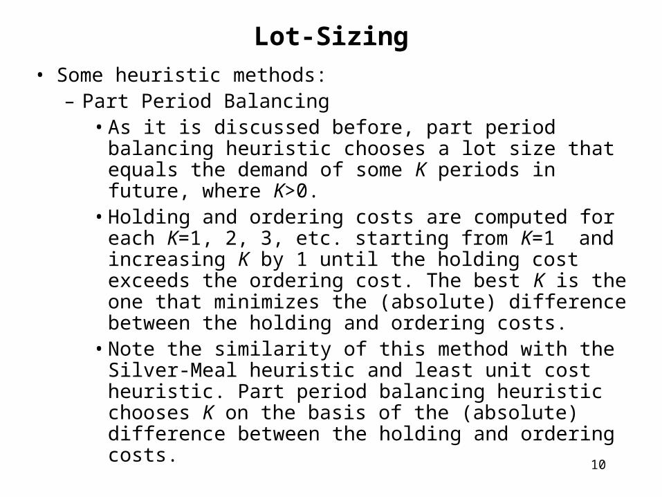
• Some heuristic methods:– Part Period Balancing
• As it is discussed before, part period balancing heuristic chooses a lot size that equals the demand of some K periods in future, where K>0.
• Holding and ordering costs are computed for each K=1, 2, 3, etc. starting from K=1 and increasing K by 1 until the holding cost exceeds the ordering cost. The best K is the one that minimizes the (absolute) difference between the holding and ordering costs.
• Note the similarity of this method with the Silver-Meal heuristic and least unit cost heuristic. Part period balancing heuristic chooses K on the basis of the (absolute) difference between the holding and ordering costs.
11
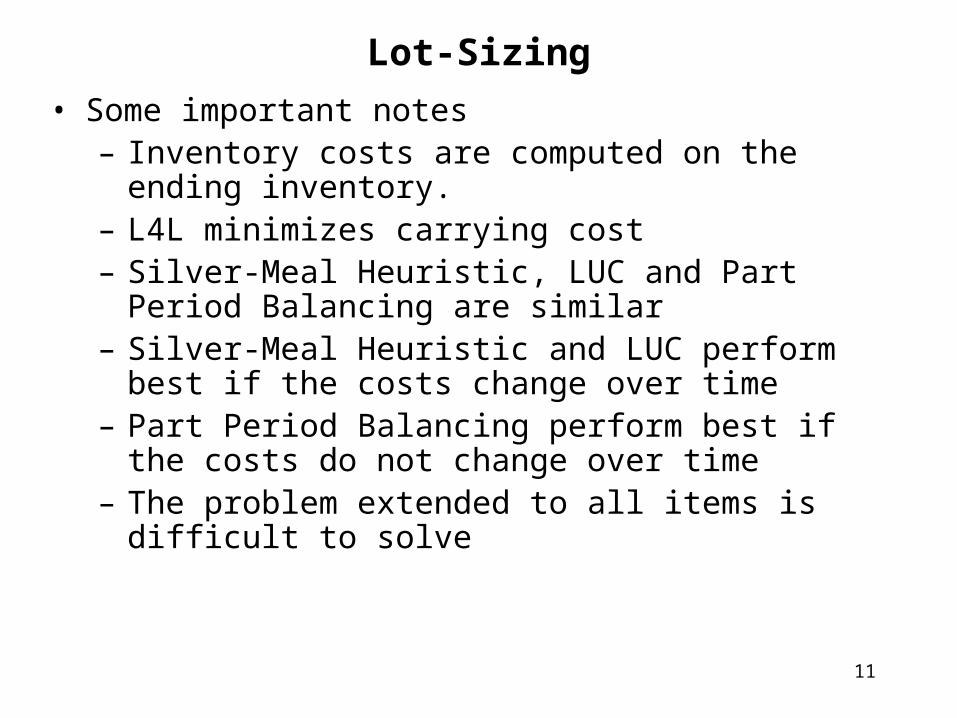
• Some important notes– Inventory costs are computed on the ending inventory.– L4L minimizes carrying cost– Silver-Meal Heuristic, LUC and Part Period Balancing
are similar– Silver-Meal Heuristic and LUC perform best if the costs
change over time– Part Period Balancing perform best if the costs do not
change over time– The problem extended to all items is difficult to solve
Lot-Sizing
12
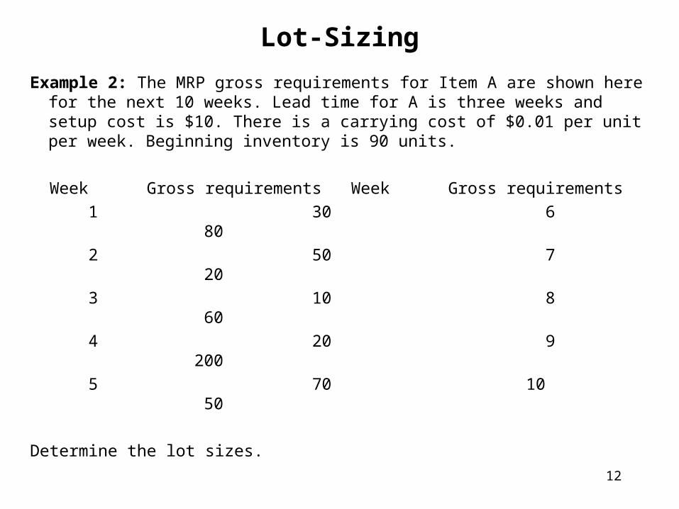
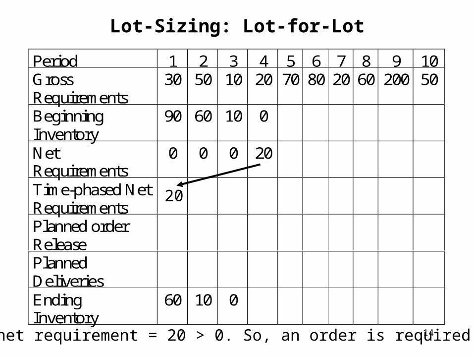
Example 2: The MRP gross requirements for Item A are shown here for the next 10 weeks. Lead time for A is three weeks and setup cost is $10. There is a carrying cost of $0.01 per unit per week. Beginning inventory is 90 units.
Week Gross requirements Week Gross requirements
1 30 6 80
2 50 7 20
3 10 8 60
4 20 9 200
5 70 10 50
Determine the lot sizes.
Lot-Sizing

13
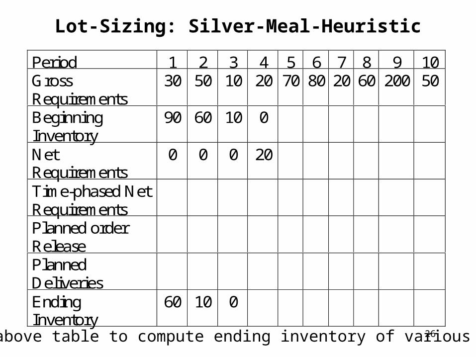
Period 1 2 3 4 5 6 7 8 9 10GrossRequirements
30 50 10 20 70 80 20 60 200 50
BeginningInventory
90 60 10 0
NetRequirements
0 0 0 20
Time-phased NetRequirementsPlanned orderReleasePlannedDeliveriesEndingInventory
60 10 0
Lot-Sizing: Lot-for-Lot
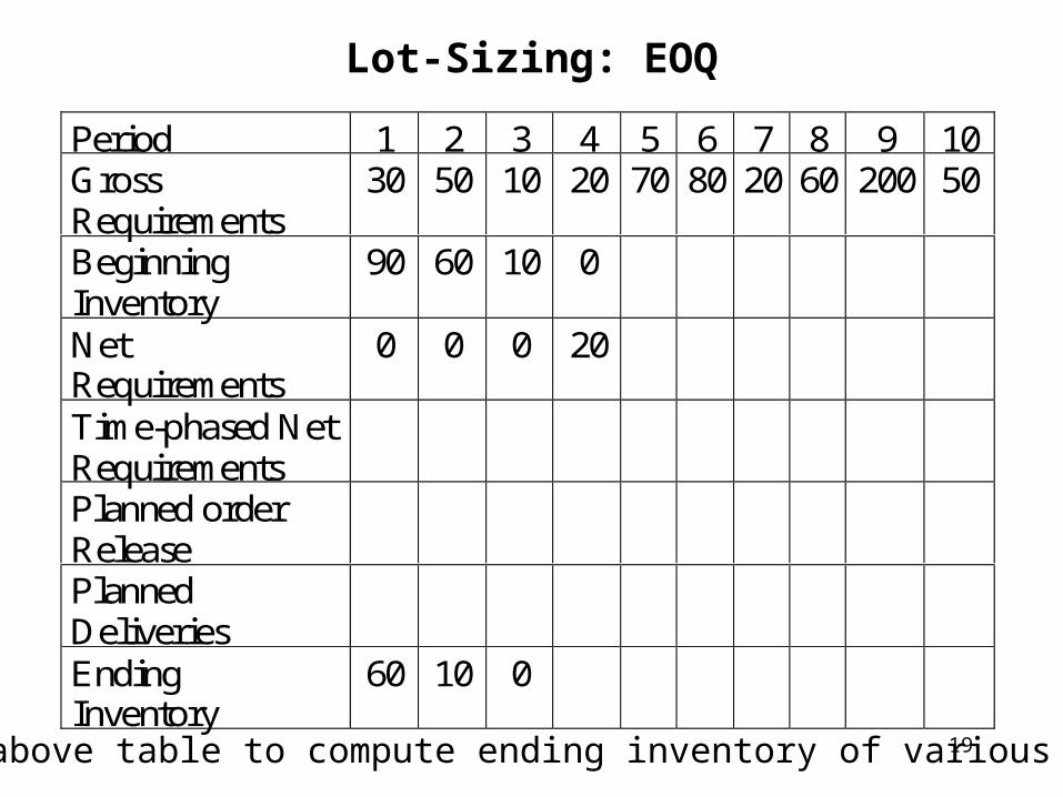
Use the above table to compute ending inventory of various periods.
14
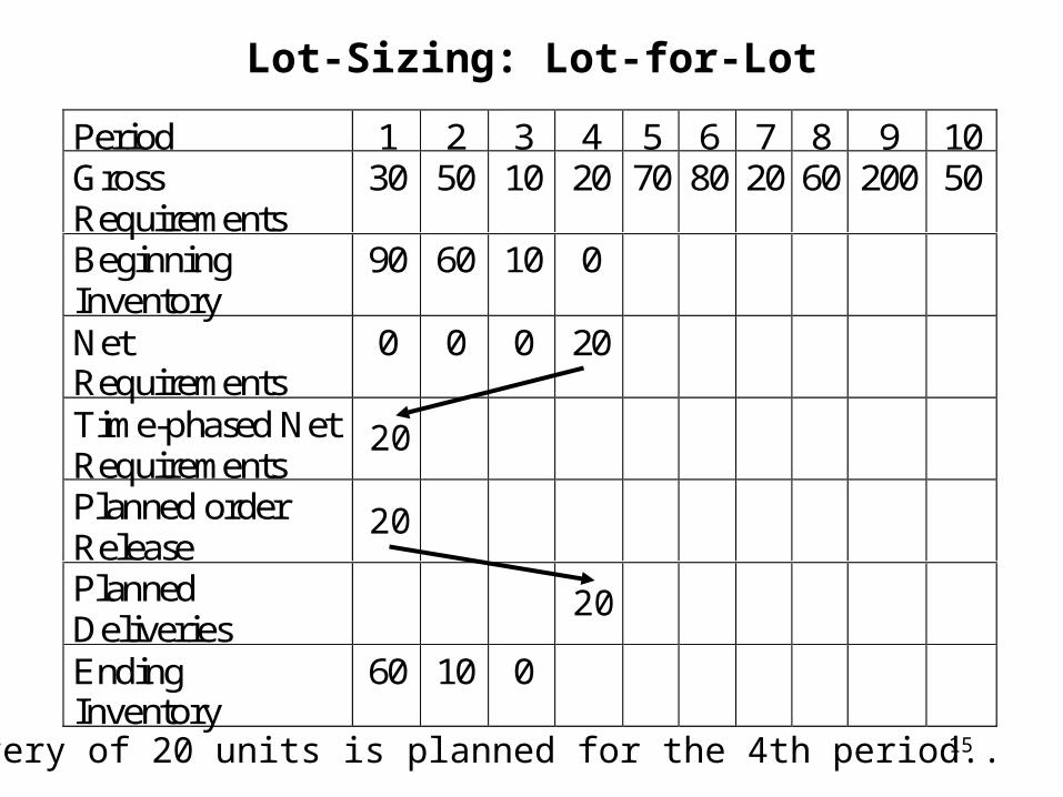
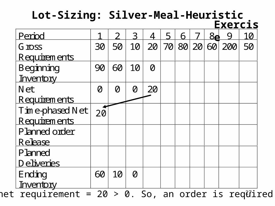
Period 1 2 3 4 5 6 7 8 9 10GrossRequirements
30 50 10 20 70 80 20 60 200 50
BeginningInventory
90 60 10 0
NetRequirements
0 0 0 20
Time-phased NetRequirementsPlanned orderReleasePlannedDeliveriesEndingInventory
60 10 0
Lot-Sizing: Lot-for-Lot
20
Week 4 net requirement = 20 > 0. So, an order is required.
15
Period 1 2 3 4 5 6 7 8 9 10GrossRequirements
30 50 10 20 70 80 20 60 200 50
BeginningInventory
90 60 10 0
NetRequirements
0 0 0 20
Time-phased NetRequirementsPlanned orderReleasePlannedDeliveriesEndingInventory
60 10 0
Lot-Sizing: Lot-for-Lot
20
20
20
A delivery of 20 units is planned for the 4th period..
16
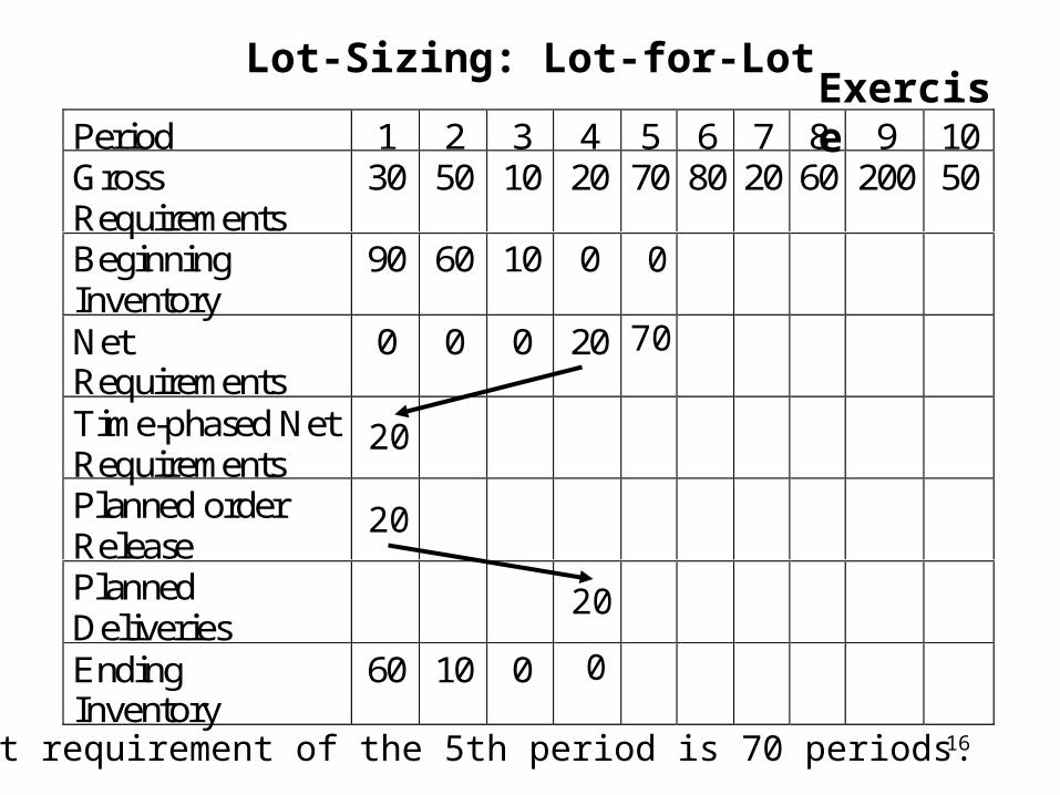
Period 1 2 3 4 5 6 7 8 9 10GrossRequirements
30 50 10 20 70 80 20 60 200 50
BeginningInventory
90 60 10 0
NetRequirements
0 0 0 20
Time-phased NetRequirementsPlanned orderReleasePlannedDeliveriesEndingInventory
60 10 0
Lot-Sizing: Lot-for-Lot
0
70
20
20
0
20
The net requirement of the 5th period is 70 periods.
Exercise
17
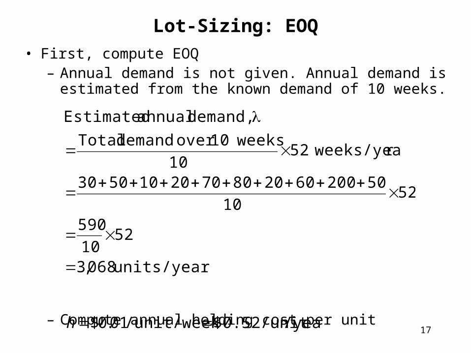
Lot-Sizing: EOQ
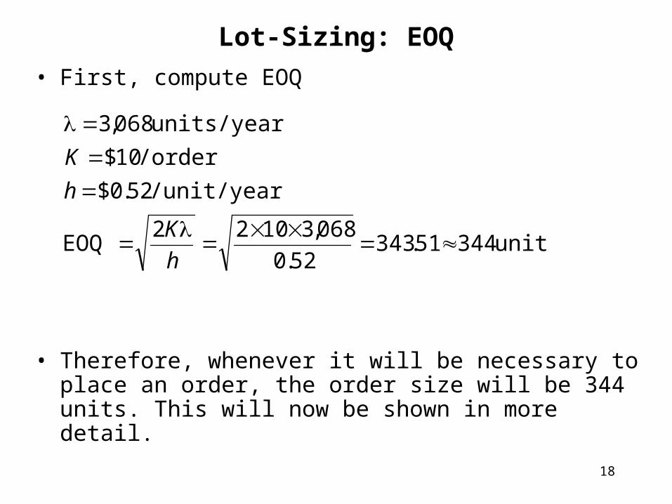
• First, compute EOQ– Annual demand is not given. Annual demand is
estimated from the known demand of 10 weeks.
– Compute annual holding cost per unit
units/year
502006020807020105030
r weeks/yea weeks10 over demand Total
demand, annual Estimated
068,3
5210
590
5210
5210
/year$0.52/unit/unit/week 01.0$h
18
Lot-Sizing: EOQ
• First, compute EOQ
• Therefore, whenever it will be necessary to place an order, the order size will be 344 units. This will now be shown in more detail.
units EOQ
/unit/year$
/order
units/year
34451.34352.0
068,31022
52.0
10$
068,3
h
K
h
K
19
Period 1 2 3 4 5 6 7 8 9 10GrossRequirements
30 50 10 20 70 80 20 60 200 50
BeginningInventory
90 60 10 0
NetRequirements
0 0 0 20
Time-phased NetRequirementsPlanned orderReleasePlannedDeliveriesEndingInventory
60 10 0
Lot-Sizing: EOQ
Use the above table to compute ending inventory of various periods.
20
Period 1 2 3 4 5 6 7 8 9 10GrossRequirements
30 50 10 20 70 80 20 60 200 50
BeginningInventory
90 60 10 0
NetRequirements
0 0 0 20
Time-phased NetRequirementsPlanned orderReleasePlannedDeliveriesEndingInventory
60 10 0
Lot-Sizing: EOQ
20
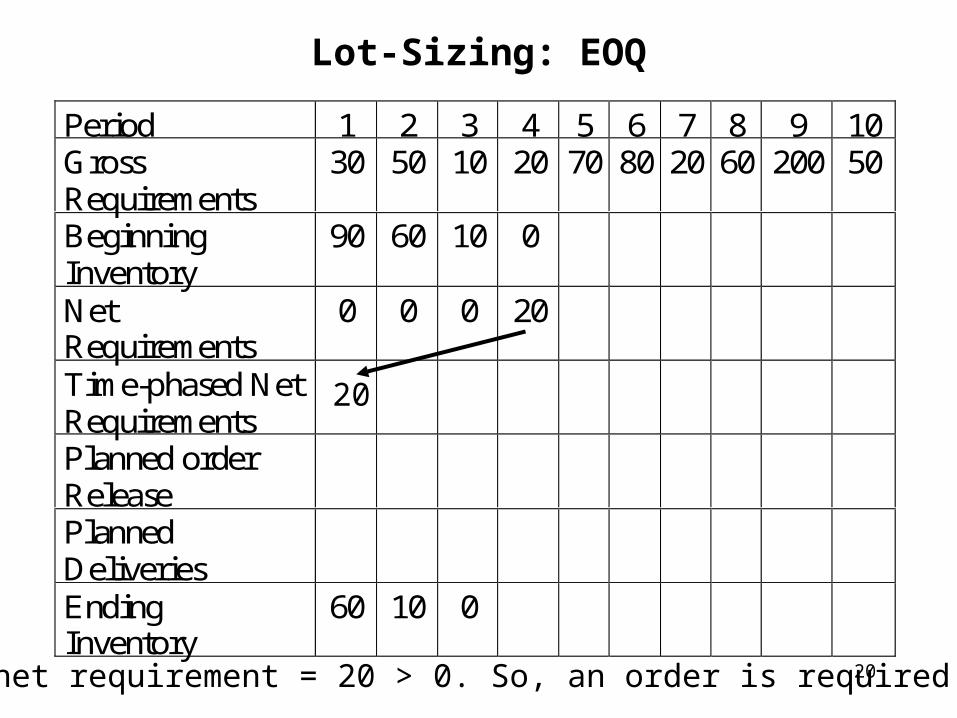
Week 4 net requirement = 20 > 0. So, an order is required.
21
Period 1 2 3 4 5 6 7 8 9 10GrossRequirements
30 50 10 20 70 80 20 60 200 50
BeginningInventory
90 60 10 0
NetRequirements
0 0 0 20
Time-phased NetRequirementsPlanned orderReleasePlannedDeliveriesEndingInventory
60 10 0
Lot-Sizing: EOQ
20
344
344
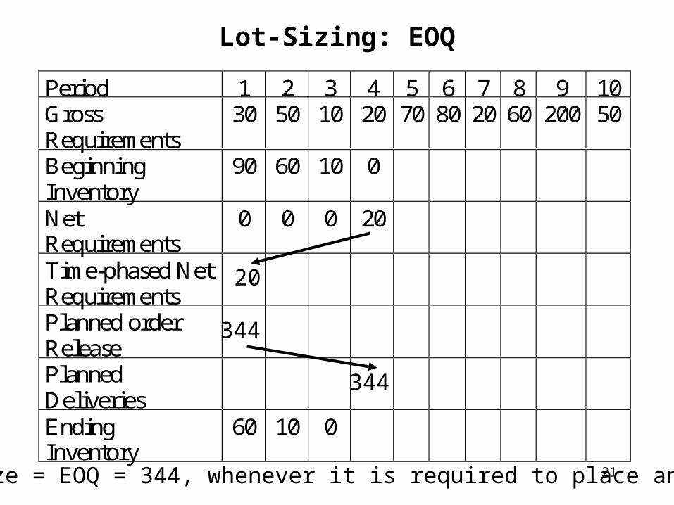
Order size = EOQ = 344, whenever it is required to place an order.
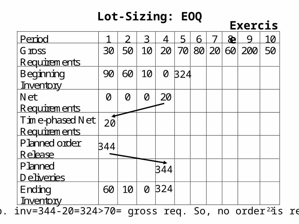
22
Period 1 2 3 4 5 6 7 8 9 10GrossRequirements
30 50 10 20 70 80 20 60 200 50
BeginningInventory
90 60 10 0
NetRequirements
0 0 0 20
Time-phased NetRequirementsPlanned orderReleasePlannedDeliveriesEndingInventory
60 10 0
Lot-Sizing: EOQ
20
344
324
344
324
Week 5 b. inv=344-20=324>70= gross req. So, no order is required.
Exercise
23
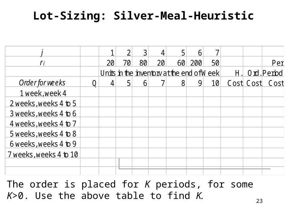
j 1 2 3 4 5 6 7r j 20 70 80 20 60 200 50 Per
H. Ord. PeriodOrder for weeks Q 4 5 6 7 8 9 10 Cost Cost Cost1 week, week 4
2 weeks, weeks 4 to 53 weeks, weeks 4 to 64 weeks, weeks 4 to 75 weeks, weeks 4 to 86 weeks, weeks 4 to 9
7 weeks, weeks 4 to 10
Units in the inventory at the end of Week
Lot-Sizing: Silver-Meal-Heuristic
The order is placed for K periods, for some K>0. Use the above table to find K.
24
j 1 2 3 4 5 6 7r j 20 70 80 20 60 200 50 Per
H. Ord. PeriodOrder for weeks Q 4 5 6 7 8 9 10 Cost Cost Cost1 week, week 4
2 weeks, weeks 4 to 53 weeks, weeks 4 to 64 weeks, weeks 4 to 75 weeks, weeks 4 to 86 weeks, weeks 4 to 9
7 weeks, weeks 4 to 10
Units in the inventory at the end of Week
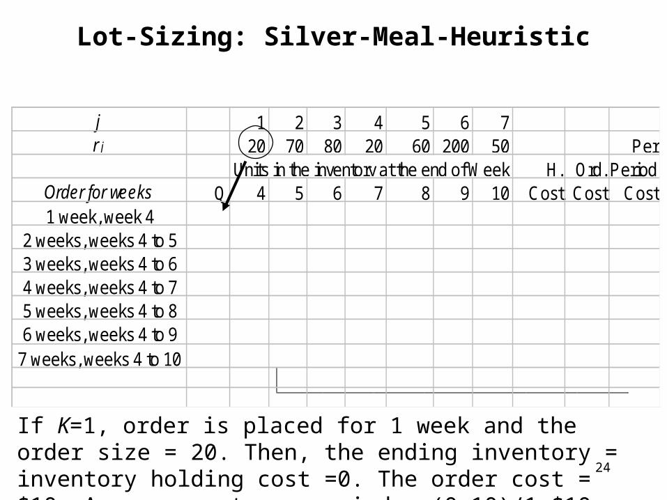
Lot-Sizing: Silver-Meal-Heuristic
20 0.00 10 10.0
If K=1, order is placed for 1 week and the order size = 20. Then, the ending inventory = inventory holding cost =0. The order cost = $10. Average cost per period = (0+10)/1=$10.
25
j 1 2 3 4 5 6 7r j 20 70 80 20 60 200 50 Per
H. Ord. PeriodOrder for weeks Q 4 5 6 7 8 9 10 Cost Cost Cost1 week, week 4
2 weeks, weeks 4 to 53 weeks, weeks 4 to 64 weeks, weeks 4 to 75 weeks, weeks 4 to 86 weeks, weeks 4 to 9
7 weeks, weeks 4 to 10
Units in the inventory at the end of Week
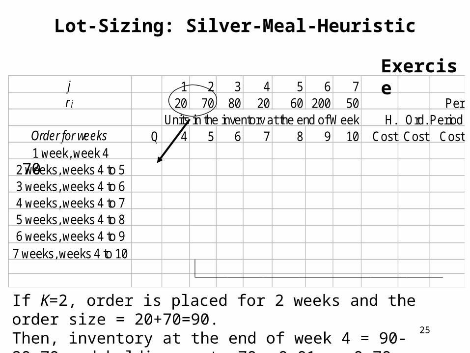
Lot-Sizing: Silver-Meal-Heuristic
20 0.00 10 10.090 70 0.70 10 5.35
If K=2, order is placed for 2 weeks and the order size = 20+70=90.Then, inventory at the end of week 4 = 90-20=70 and holding cost =70 0.01. = 0.70. Average cost per period = (0.70+10)/2=$5.35.
Exercise
26
Period 1 2 3 4 5 6 7 8 9 10GrossRequirements
30 50 10 20 70 80 20 60 200 50
BeginningInventory
90 60 10 0
NetRequirements
0 0 0 20
Time-phased NetRequirementsPlanned orderReleasePlannedDeliveriesEndingInventory
60 10 0
Lot-Sizing: Silver-Meal-Heuristic
Use the above table to compute ending inventory of various periods.
27
Period 1 2 3 4 5 6 7 8 9 10GrossRequirements
30 50 10 20 70 80 20 60 200 50
BeginningInventory
90 60 10 0
NetRequirements
0 0 0 20
Time-phased NetRequirementsPlanned orderReleasePlannedDeliveriesEndingInventory
60 10 0
Lot-Sizing: Silver-Meal-Heuristic
20
Week 4 net requirement = 20 > 0. So, an order is required.
Exercise
28
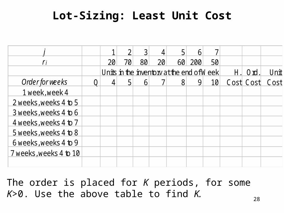
j 1 2 3 4 5 6 7r j 20 70 80 20 60 200 50
H. Ord. UnitOrder for weeks Q 4 5 6 7 8 9 10 Cost Cost Cost1 week, week 4
2 weeks, weeks 4 to 53 weeks, weeks 4 to 64 weeks, weeks 4 to 75 weeks, weeks 4 to 86 weeks, weeks 4 to 9
7 weeks, weeks 4 to 10
Units in the inventory at the end of Week
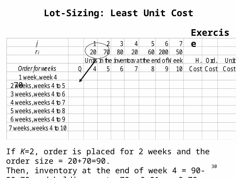
Lot-Sizing: Least Unit Cost
The order is placed for K periods, for some K>0. Use the above table to find K.
29
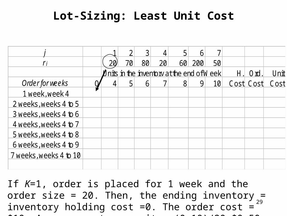
j 1 2 3 4 5 6 7r j 20 70 80 20 60 200 50
H. Ord. UnitOrder for weeks Q 4 5 6 7 8 9 10 Cost Cost Cost1 week, week 4
2 weeks, weeks 4 to 53 weeks, weeks 4 to 64 weeks, weeks 4 to 75 weeks, weeks 4 to 86 weeks, weeks 4 to 9
7 weeks, weeks 4 to 10
Units in the inventory at the end of Week
Lot-Sizing: Least Unit Cost
20 0.00 10 .500
If K=1, order is placed for 1 week and the order size = 20. Then, the ending inventory = inventory holding cost =0. The order cost = $10. Average cost per unit = (0+10)/20=$0.50
30
j 1 2 3 4 5 6 7r j 20 70 80 20 60 200 50
H. Ord. UnitOrder for weeks Q 4 5 6 7 8 9 10 Cost Cost Cost1 week, week 4
2 weeks, weeks 4 to 53 weeks, weeks 4 to 64 weeks, weeks 4 to 75 weeks, weeks 4 to 86 weeks, weeks 4 to 9
7 weeks, weeks 4 to 10
Units in the inventory at the end of Week
Lot-Sizing: Least Unit Cost
20 0.00 10 .50090 70 0.70 10 .119
If K=2, order is placed for 2 weeks and the order size = 20+70=90.Then, inventory at the end of week 4 = 90-20=70 and holding cost =70 0.01. = 0.70. Average cost per unit = (0.70+10)/90=$0.119.
Exercise
31
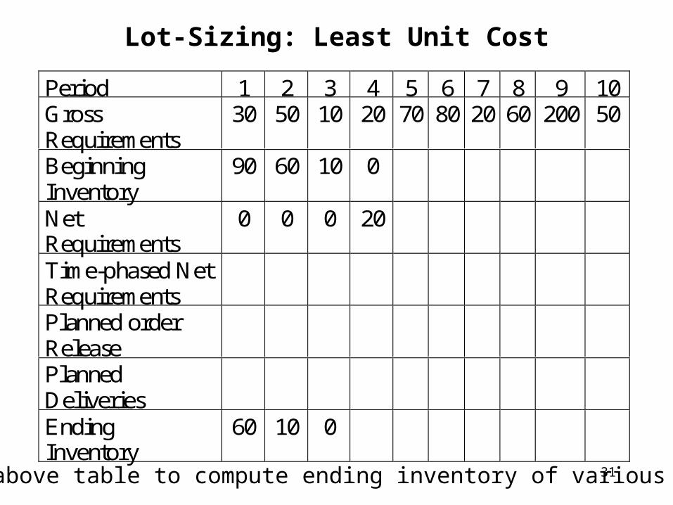
Lot-Sizing: Least Unit Cost
Period 1 2 3 4 5 6 7 8 9 10GrossRequirements
30 50 10 20 70 80 20 60 200 50
BeginningInventory
90 60 10 0
NetRequirements
0 0 0 20
Time-phased NetRequirementsPlanned orderReleasePlannedDeliveriesEndingInventory
60 10 0
Use the above table to compute ending inventory of various periods.
32
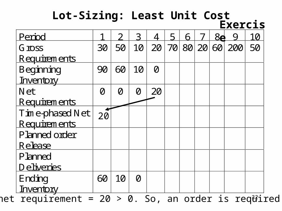
Lot-Sizing: Least Unit Cost
Period 1 2 3 4 5 6 7 8 9 10GrossRequirements
30 50 10 20 70 80 20 60 200 50
BeginningInventory
90 60 10 0
NetRequirements
0 0 0 20
Time-phased NetRequirementsPlanned orderReleasePlannedDeliveriesEndingInventory
60 10 0
20
Week 4 net requirement = 20 > 0. So, an order is required.
Exercise
33
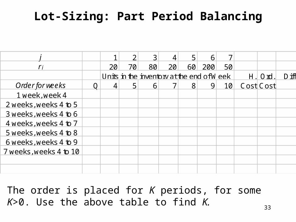
Lot-Sizing: Part Period Balancing
j 1 2 3 4 5 6 7r j 20 70 80 20 60 200 50
H. Ord. DiffOrder for weeks Q 4 5 6 7 8 9 10 Cost Cost1 week, week 4
2 weeks, weeks 4 to 53 weeks, weeks 4 to 64 weeks, weeks 4 to 75 weeks, weeks 4 to 86 weeks, weeks 4 to 9
7 weeks, weeks 4 to 10
Units in the inventory at the end of Week
The order is placed for K periods, for some K>0. Use the above table to find K.
34
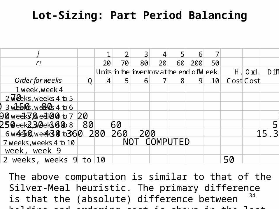
Lot-Sizing: Part Period Balancing
j 1 2 3 4 5 6 7r j 20 70 80 20 60 200 50
H. Ord. DiffOrder for weeks Q 4 5 6 7 8 9 10 Cost Cost1 week, week 4
2 weeks, weeks 4 to 53 weeks, weeks 4 to 64 weeks, weeks 4 to 75 weeks, weeks 4 to 86 weeks, weeks 4 to 9
7 weeks, weeks 4 to 10
Units in the inventory at the end of Week
20 0.00 10 10.090 70 0.70 10 9.30
170 150 80 2.30 10 7.70190 170 100 20 2.90 10 7.10250 230 160 80 60 5.30 10 4.70450 430 360 280 260 200 15.30 10 5.30
NOT COMPUTED1 week, week 92 weeks, weeks 9 to 10
200 0.00 10 10.0250 50 0.50 10 9.50
The above computation is similar to that of the Silver-Meal heuristic. The primary difference is that the (absolute) difference between holding and ordering cost is shown in the last column.
35
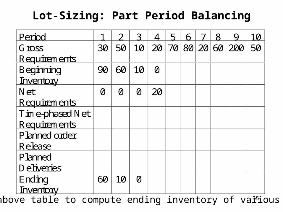
Lot-Sizing: Part Period Balancing
Period 1 2 3 4 5 6 7 8 9 10GrossRequirements
30 50 10 20 70 80 20 60 200 50
BeginningInventory
90 60 10 0
NetRequirements
0 0 0 20
Time-phased NetRequirementsPlanned orderReleasePlannedDeliveriesEndingInventory
60 10 0
Use the above table to compute ending inventory of various periods.
36
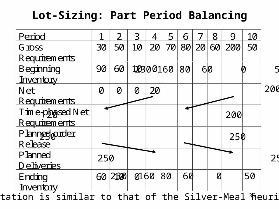
Lot-Sizing: Part Period Balancing
Period 1 2 3 4 5 6 7 8 9 10GrossRequirements
30 50 10 20 70 80 20 60 200 50
BeginningInventory
90 60 10 0
NetRequirements
0 0 0 20
Time-phased NetRequirementsPlanned orderReleasePlannedDeliveriesEndingInventory
60 10 0
200
20 200
250 250
230 160 80 60 0 50 0
250 250
230 160 80 60 0 50
The computation is similar to that of the Silver-Meal heuristic.
37
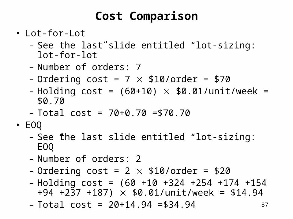
• Lot-for-Lot– See the last slide entitled “lot-sizing: lot-for-lot”– Number of orders: 7– Ordering cost = 7 $10/order = $70– Holding cost = (60+10) $0.01/unit/week = $0.70– Total cost = 70+0.70 =$70.70
• EOQ– See the last slide entitled “lot-sizing: EOQ”– Number of orders: 2– Ordering cost = 2 $10/order = $20– Holding cost = (60 +10 +324 +254 +174 +154 +94
+237 +187) $0.01/unit/week = $14.94– Total cost = 20+14.94 =$34.94
Cost Comparison

38
• Silver-Meal Heuristic– See the last slide entitled “lot-sizing: Silver-Meal
heuristic”– Number of orders: 2– Ordering cost = 2 $10/order = $20– Holding cost = (60 +10 +230 +160 +80 +60 +50)
$0.01/unit/week = $6.50– Total cost = 20+6.50 =$26.50
• Least Unit Cost– See the last slide entitled “lot-sizing: least unit cost”– Number of orders: 2– Ordering cost = 2 $10/order = $20– Holding cost = (60 +10 +430 +360 +280 +260 +200)
$0.01/unit/week = $16.00– Total cost = 20+16.00 =$36.00
Cost Comparison
39
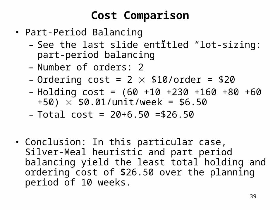
• Part-Period Balancing– See the last slide entitled “lot-sizing: part-period
balancing”– Number of orders: 2– Ordering cost = 2 $10/order = $20– Holding cost = (60 +10 +230 +160 +80 +60 +50)
$0.01/unit/week = $6.50– Total cost = 20+6.50 =$26.50
• Conclusion: In this particular case, Silver-Meal heuristic and part period balancing yield the least total holding and ordering cost of $26.50 over the planning period of 10 weeks.
Cost Comparison
40
READING AND EXERCISES
Lesson 22
Reading:
Section 7.2-7.3 pp. 366-375 (4th Ed.), pp. 358-366 (5th Ed.)
Exercise:
17 and 25 pp. 371-373, 375 (4th Ed.), pp. 363, 366