Embed Size (px)
Citation preview
Analysis of Time-series DataGeneralized Additive Model
Jinseob Kim
July 17, 2015
Jinseob Kim Analysis of Time-series Data July 17, 2015 1 / 45
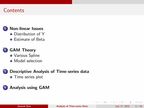
Contents
1 Non-linear IssuesDistribution of YEstimate of Beta
2 GAM TheoryVarious SplineModel selection
3 Descriptive Analysis of Time-series dataTime series plot
4 Analysis using GAM
Jinseob Kim Analysis of Time-series Data July 17, 2015 2 / 45

Objective
1 Non-linear regression의 종류를 안다.
2 Additive model의 개념과 spline에 대해 이해한다.
3 Time-series data를 살펴볼 줄 안다.
4 R의 mgcv 패키지를 이용하여 분석을 시행할 수 있다.
Jinseob Kim Analysis of Time-series Data July 17, 2015 3 / 45
Non-linear Issues
Contents
1 Non-linear IssuesDistribution of YEstimate of Beta
2 GAM TheoryVarious SplineModel selection
3 Descriptive Analysis of Time-series dataTime series plot
4 Analysis using GAM
Jinseob Kim Analysis of Time-series Data July 17, 2015 4 / 45
Non-linear Issues Distribution of Y
Count data
일/주/월 별 발생/사망 수
Population의 경향을 바라본다. 나랏님 시점!!
인구집단에서 발생 or 사망할 확률이 어느정도냐?
확률
정규분포
포아송분포
기타..quasipoisson, Gamma, Negbin, ZIP, ZINB...
매우 중요하다!!! p-value가 바뀐다!!!
Jinseob Kim Analysis of Time-series Data July 17, 2015 5 / 45
Non-linear Issues Distribution of Y
Compare Distribution
http://resources.esri.com/help/9.3/arcgisdesktop/com/gp_
toolref/process_simulations_sensitivity_analysis_and_error_
analysis_modeling/distributions_for_assigning_random_
values.htm
Jinseob Kim Analysis of Time-series Data July 17, 2015 6 / 45
Non-linear Issues Distribution of Y
기초수준
흔한 질병이면 정규분포 고려. 분석 쉬워진다.
드문 질병이면 포아송.
평균 < 분산? → quasipoisson
나머지는 드물게 쓰인다.
Jinseob Kim Analysis of Time-series Data July 17, 2015 7 / 45
Non-linear Issues Distribution of Y
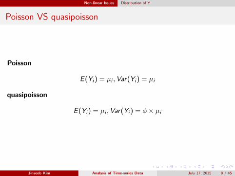
Poisson VS quasipoisson
Poisson
E (Yi ) = µi ,Var(Yi ) = µi
quasipoisson
E (Yi ) = µi ,Var(Yi ) = φ× µi
Jinseob Kim Analysis of Time-series Data July 17, 2015 8 / 45
Non-linear Issues Estimate of Beta
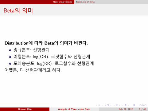
Beta의 의미
Distribution에 따라 Beta의 의미가 바뀐다.
정규분포: 선형관계
이항분포: log(OR)- 로짓함수와 선형관계
포아송분포: log(RR)- 로그함수와 선형관계
어쨌든, 다 선형관계라고 하자.
Jinseob Kim Analysis of Time-series Data July 17, 2015 9 / 45
Non-linear Issues Estimate of Beta
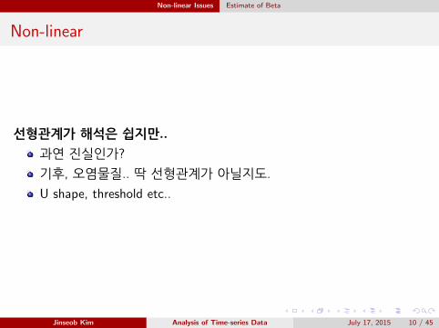
Non-linear
선형관계가 해석은 쉽지만..
과연 진실인가?
기후, 오염물질.. 딱 선형관계가 아닐지도.
U shape, threshold etc..
Jinseob Kim Analysis of Time-series Data July 17, 2015 10 / 45
GAM Theory
Contents
1 Non-linear IssuesDistribution of YEstimate of Beta
2 GAM TheoryVarious SplineModel selection
3 Descriptive Analysis of Time-series dataTime series plot
4 Analysis using GAM
Jinseob Kim Analysis of Time-series Data July 17, 2015 11 / 45
GAM Theory Various Spline
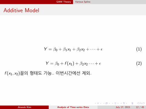
Additive Model
Y = β0 + β1x1 + β2x2 + · · ·+ ε (1)
Y = β0 + f (x1) + β2x2 · · ·+ ε (2)
f (x1, x2)꼴의 형태도 가능.. 이번시간에선 제외.
Jinseob Kim Analysis of Time-series Data July 17, 2015 12 / 45
GAM Theory Various Spline
Determine f
종류
Loess
(Natural)Cubic spline
Smoothing spline
내용은 다양하지만.. 실제 결과는 거의 비슷.
Jinseob Kim Analysis of Time-series Data July 17, 2015 13 / 45
GAM Theory Various Spline
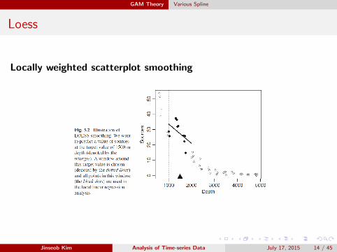
Loess
Locally weighted scatterplot smoothing
Jinseob Kim Analysis of Time-series Data July 17, 2015 14 / 45
GAM Theory Various Spline
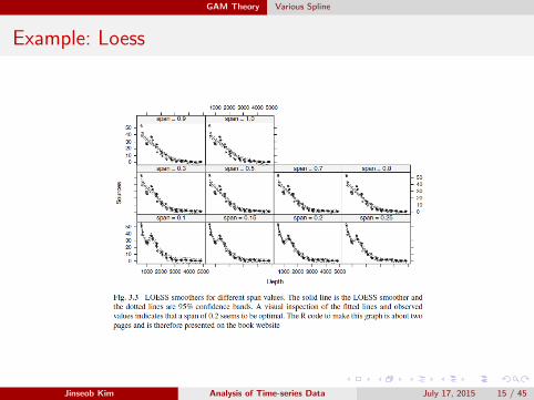
Example: Loess
Jinseob Kim Analysis of Time-series Data July 17, 2015 15 / 45
GAM Theory Various Spline
Cubic spline
Cubic = 3차방정식
구간을 몇개로 나누고: knot
각 구간을 3차방정식을 이용하여 모델링.
구간 사이에 smoothing 고려..
Jinseob Kim Analysis of Time-series Data July 17, 2015 16 / 45
GAM Theory Various Spline
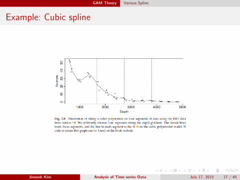
Example: Cubic spline
Jinseob Kim Analysis of Time-series Data July 17, 2015 17 / 45
GAM Theory Various Spline
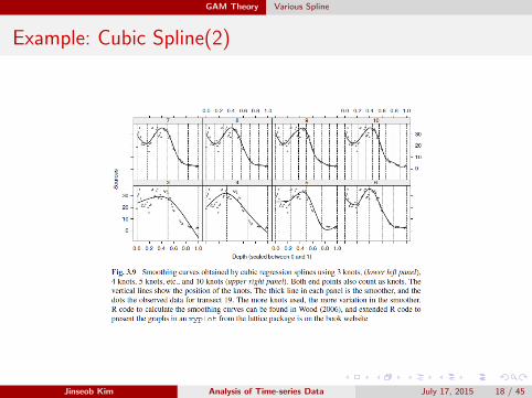
Example: Cubic Spline(2)
Jinseob Kim Analysis of Time-series Data July 17, 2015 18 / 45
GAM Theory Various Spline
Natural cubic spline: ns
Cubic + 처음과 끝은 Linear
처음보다 더 처음, 끝보다 더 끝(데이터에 없는 숫자)에 대한 보수적인추정.
3차보다 1차가 변화량이 적음.
Jinseob Kim Analysis of Time-series Data July 17, 2015 19 / 45
GAM Theory Various Spline
Smoothing Splines Alias Penalised Splines
Loess, Cubic spline
Span, knot를 미리 지정: local 구간을 미리 지정.
Penalized spline
알아서.. 데이터가 말해주는 대로..
mgcv R 패키지의 기본옵션.
Jinseob Kim Analysis of Time-series Data July 17, 2015 20 / 45
GAM Theory Various Spline
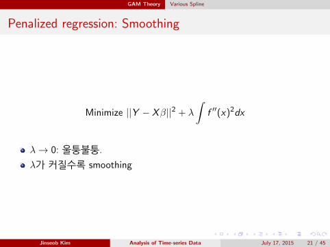
Penalized regression: Smoothing
Minimize ||Y − Xβ||2 + λ
∫f ′′(x)2dx
λ→ 0: 울퉁불퉁.
λ가 커질수록 smoothing
Jinseob Kim Analysis of Time-series Data July 17, 2015 21 / 45
GAM Theory Various Spline
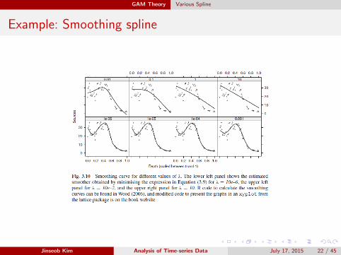
Example: Smoothing spline
Jinseob Kim Analysis of Time-series Data July 17, 2015 22 / 45
GAM Theory Model selection
Choose λ
1 CV (cross validation)
2 GCV (generalized)
3 UBRE (unbiased risk estimator)
4 Mallow’s Cp
어떤 것이든.. 최소로 하는 λ를 choose!!
Jinseob Kim Analysis of Time-series Data July 17, 2015 23 / 45
GAM Theory Model selection
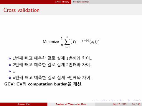
Cross validation
Minimize1
n
n∑i=1
(Yi − f̂ −[i ](xi ))2
1번째 빼고 예측한 걸로 실제 1번째와 차이..
2번째 빼고 예측한 걸로 실제 2번째와 차이..
..
n번째 빼고 예측한 걸로 실제 n번째와 차이..
GCV: CV의 computation burden을 개선.
Jinseob Kim Analysis of Time-series Data July 17, 2015 24 / 45
GAM Theory Model selection
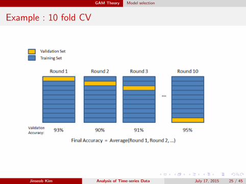
Example : 10 fold CV
Jinseob Kim Analysis of Time-series Data July 17, 2015 25 / 45
GAM Theory Model selection
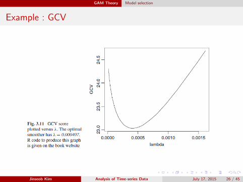
Example : GCV
Jinseob Kim Analysis of Time-series Data July 17, 2015 26 / 45
GAM Theory Model selection
In practice
poisson: UBRE
quasipoisson: GCV
Jinseob Kim Analysis of Time-series Data July 17, 2015 27 / 45
GAM Theory Model selection
AIC
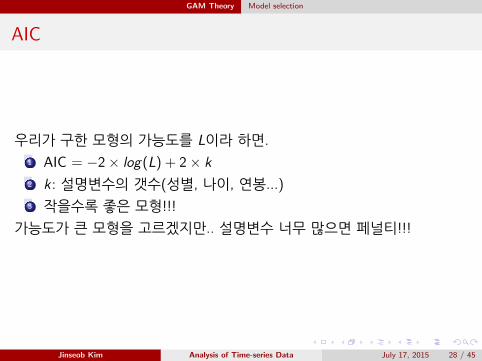
우리가 구한 모형의 가능도를 L이라 하면.
1 AIC = −2× log(L) + 2× k
2 k: 설명변수의 갯수(성별, 나이, 연봉...)
3 작을수록 좋은 모형!!!
가능도가 큰 모형을 고르겠지만.. 설명변수 너무 많으면 페널티!!!
Jinseob Kim Analysis of Time-series Data July 17, 2015 28 / 45
Descriptive Analysis of Time-series data
Contents
1 Non-linear IssuesDistribution of YEstimate of Beta
2 GAM TheoryVarious SplineModel selection
3 Descriptive Analysis of Time-series dataTime series plot
4 Analysis using GAM
Jinseob Kim Analysis of Time-series Data July 17, 2015 29 / 45
Descriptive Analysis of Time-series data Time series plot
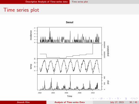
Time series plot
01
23
45
inci
denc
e
1020
0000
1030
0000
popu
latio
n
010
2030
tem
p
020
040
0
2002 2004 2006 2008 2010
pcp
Time
Seoul
Jinseob Kim Analysis of Time-series Data July 17, 2015 30 / 45
Descriptive Analysis of Time-series data Time series plot
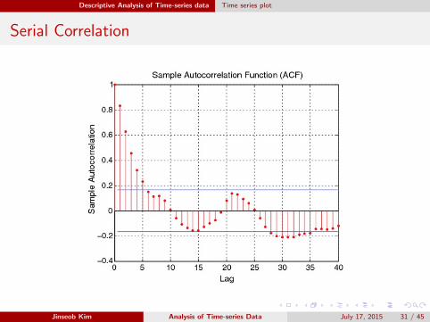
Serial Correlation
Jinseob Kim Analysis of Time-series Data July 17, 2015 31 / 45
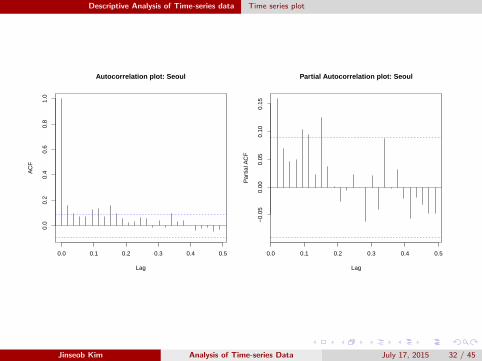
Descriptive Analysis of Time-series data Time series plot
0.0 0.1 0.2 0.3 0.4 0.5
0.0
0.2
0.4
0.6
0.8
1.0
Lag
AC
F
Autocorrelation plot: Seoul
0.0 0.1 0.2 0.3 0.4 0.5−
0.05
0.00
0.05
0.10
0.15
Lag
Par
tial A
CF
Partial Autocorrelation plot: Seoul
Jinseob Kim Analysis of Time-series Data July 17, 2015 32 / 45
Descriptive Analysis of Time-series data Time series plot
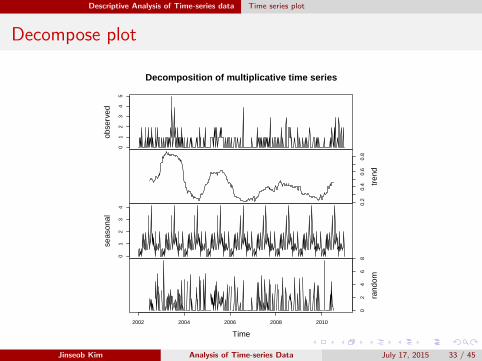
Decompose plot
01
23
45
obse
rved
0.2
0.4
0.6
0.8
tren
d
01
23
4
seas
onal
02
46
8
2002 2004 2006 2008 2010
rand
om
Time
Decomposition of multiplicative time series
Jinseob Kim Analysis of Time-series Data July 17, 2015 33 / 45
Analysis using GAM
Contents
1 Non-linear IssuesDistribution of YEstimate of Beta
2 GAM TheoryVarious SplineModel selection
3 Descriptive Analysis of Time-series dataTime series plot
4 Analysis using GAM
Jinseob Kim Analysis of Time-series Data July 17, 2015 34 / 45
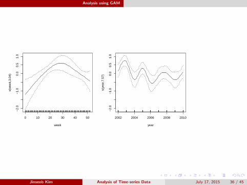
Analysis using GAM
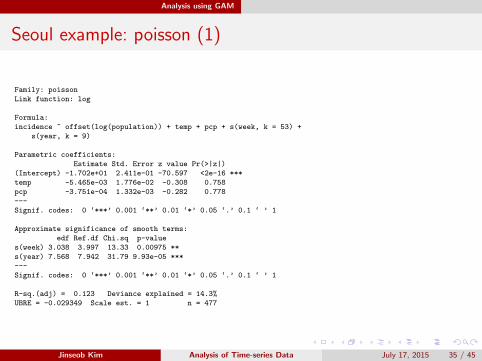
Seoul example: poisson (1)
Family: poisson
Link function: log
Formula:
incidence ~ offset(log(population)) + temp + pcp + s(week, k = 53) +
s(year, k = 9)
Parametric coefficients:
Estimate Std. Error z value Pr(>|z|)
(Intercept) -1.702e+01 2.411e-01 -70.597 <2e-16 ***
temp -5.465e-03 1.776e-02 -0.308 0.758
pcp -3.751e-04 1.332e-03 -0.282 0.778
---
Signif. codes: 0 ‘***’ 0.001 ‘**’ 0.01 ‘*’ 0.05 ‘.’ 0.1 ‘ ’ 1
Approximate significance of smooth terms:
edf Ref.df Chi.sq p-value
s(week) 3.038 3.997 13.33 0.00975 **
s(year) 7.568 7.942 31.79 9.93e-05 ***
---
Signif. codes: 0 ‘***’ 0.001 ‘**’ 0.01 ‘*’ 0.05 ‘.’ 0.1 ‘ ’ 1
R-sq.(adj) = 0.123 Deviance explained = 14.3%
UBRE = -0.029349 Scale est. = 1 n = 477
Jinseob Kim Analysis of Time-series Data July 17, 2015 35 / 45
Analysis using GAM
0 10 20 30 40 50
−2.
0−
1.0
0.0
0.5
1.0
week
s(w
eek,
3.04
)
2002 2004 2006 2008 2010
−2.
0−
1.0
0.0
0.5
1.0
year
s(ye
ar,7
.57)
Jinseob Kim Analysis of Time-series Data July 17, 2015 36 / 45

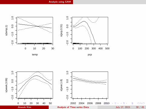
Analysis using GAM
Seoul example: poisson (2)
Family: poisson
Link function: log
Formula:
incidence ~ offset(log(population)) + s(temp) + s(pcp) + s(week,
k = 53) + s(year, k = 9)
Parametric coefficients:
Estimate Std. Error z value Pr(>|z|)
(Intercept) -17.07888 0.07856 -217.4 <2e-16 ***
---
Signif. codes: 0 ‘***’ 0.001 ‘**’ 0.01 ‘*’ 0.05 ‘.’ 0.1 ‘ ’ 1
Approximate significance of smooth terms:
edf Ref.df Chi.sq p-value
s(temp) 1.000 1.000 0.538 0.46313
s(pcp) 3.312 4.142 7.036 0.14440
s(week) 3.063 4.030 14.319 0.00654 **
s(year) 1.798 2.236 6.634 0.04593 *
---
Signif. codes: 0 ‘***’ 0.001 ‘**’ 0.01 ‘*’ 0.05 ‘.’ 0.1 ‘ ’ 1
R-sq.(adj) = 0.0834 Deviance explained = 11.5%
UBRE = -0.014142 Scale est. = 1 n = 477
Jinseob Kim Analysis of Time-series Data July 17, 2015 37 / 45
Analysis using GAM
0 10 20 30
−2.
0−
1.0
0.0
1.0
temp
s(te
mp,
1)
0 100 200 300 400 500
−2.
0−
1.0
0.0
1.0
pcp
s(pc
p,3.
31)
0 10 20 30 40 50
−2.
0−
1.0
0.0
1.0
week
s(w
eek,
3.06
)
2002 2004 2006 2008 2010
−2.
0−
1.0
0.0
1.0
year
s(ye
ar,1
.8)
Jinseob Kim Analysis of Time-series Data July 17, 2015 38 / 45
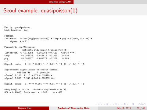
Analysis using GAM
Seoul example: quasipoisson(1)
Family: quasipoisson
Link function: log
Formula:
incidence ~ offset(log(population)) + temp + pcp + s(week, k = 53) +
s(year, k = 9)
Parametric coefficients:
Estimate Std. Error t value Pr(>|t|)
(Intercept) -17.012052 0.252254 -67.440 <2e-16 ***
temp -0.006425 0.018615 -0.345 0.730
pcp -0.000377 0.001378 -0.274 0.785
---
Signif. codes: 0 ‘***’ 0.001 ‘**’ 0.01 ‘*’ 0.05 ‘.’ 0.1 ‘ ’ 1
Approximate significance of smooth terms:
edf Ref.df F p-value
s(week) 3.126 4.110 3.072 0.015470 *
s(year) 7.595 7.949 3.746 0.000303 ***
---
Signif. codes: 0 ‘***’ 0.001 ‘**’ 0.01 ‘*’ 0.05 ‘.’ 0.1 ‘ ’ 1
R-sq.(adj) = 0.124 Deviance explained = 14.3%
GCV = 0.96803 Scale est. = 1.068 n = 477
Jinseob Kim Analysis of Time-series Data July 17, 2015 39 / 45

Analysis using GAM
0 10 20 30 40 50
−2.
0−
1.0
0.0
0.5
1.0
week
s(w
eek,
3.13
)
2002 2004 2006 2008 2010
−2.
0−
1.0
0.0
0.5
1.0
year
s(ye
ar,7
.59)
Jinseob Kim Analysis of Time-series Data July 17, 2015 40 / 45
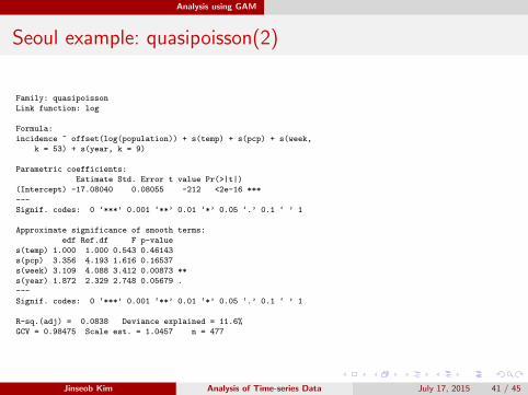
Analysis using GAM
Seoul example: quasipoisson(2)
Family: quasipoisson
Link function: log
Formula:
incidence ~ offset(log(population)) + s(temp) + s(pcp) + s(week,
k = 53) + s(year, k = 9)
Parametric coefficients:
Estimate Std. Error t value Pr(>|t|)
(Intercept) -17.08040 0.08055 -212 <2e-16 ***
---
Signif. codes: 0 ‘***’ 0.001 ‘**’ 0.01 ‘*’ 0.05 ‘.’ 0.1 ‘ ’ 1
Approximate significance of smooth terms:
edf Ref.df F p-value
s(temp) 1.000 1.000 0.543 0.46143
s(pcp) 3.356 4.193 1.616 0.16537
s(week) 3.109 4.088 3.412 0.00873 **
s(year) 1.872 2.329 2.748 0.05679 .
---
Signif. codes: 0 ‘***’ 0.001 ‘**’ 0.01 ‘*’ 0.05 ‘.’ 0.1 ‘ ’ 1
R-sq.(adj) = 0.0838 Deviance explained = 11.6%
GCV = 0.98475 Scale est. = 1.0457 n = 477
Jinseob Kim Analysis of Time-series Data July 17, 2015 41 / 45

Analysis using GAM
0 10 20 30
−2.
0−
1.0
0.0
1.0
temp
s(te
mp,
1)
0 100 200 300 400 500
−2.
0−
1.0
0.0
1.0
pcp
s(pc
p,3.
36)
0 10 20 30 40 50
−2.
0−
1.0
0.0
1.0
week
s(w
eek,
3.11
)
2002 2004 2006 2008 2010
−2.
0−
1.0
0.0
1.0
year
s(ye
ar,1
.87)
Jinseob Kim Analysis of Time-series Data July 17, 2015 42 / 45
Analysis using GAM
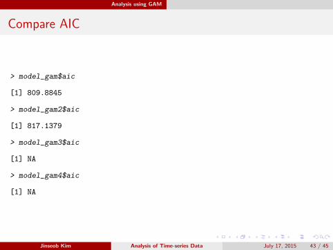
Compare AIC
> model_gam$aic
[1] 809.8845
> model_gam2$aic
[1] 817.1379
> model_gam3$aic
[1] NA
> model_gam4$aic
[1] NA
Jinseob Kim Analysis of Time-series Data July 17, 2015 43 / 45
Analysis using GAM
Good reference
Using R for Time Series Analysishttp://a-little-book-of-r-for-time-series.readthedocs.org/
en/latest/
Jinseob Kim Analysis of Time-series Data July 17, 2015 44 / 45
Analysis using GAM
END
Email : [email protected]
Jinseob Kim Analysis of Time-series Data July 17, 2015 45 / 45