Constrained Generalized Additive Modelwith Zero-Inflated Data

Hai Liu

The University of Iowa, Iowa City, U.S.A.

Kung-Sik Chan †

The University of Iowa, Iowa City, U.S.A.

Summary. Zero inflation problem is very common in ecological studies as well as other areas.We propose the COnstrained Zero-Inflated Generalized Additive Model (COZIGAM) for analyz-ing zero-inflated data. Our approach assumes that the response follows some distribution fromthe zero-inflated 1-parameter exponential family, with the further assumption that the probabil-ity of zero inflation is some monotone function of the mean response function. When the latterassumption obtains, the new approach provides a unified framework for modeling zero-inflateddata. This bypasses the problems of two popular methods for analyzing zero-inflated data thateither focus only on the non-zero data or model the presence-absence data and the non-zerodata separately. We develop an iterative algorithm for penalized likelihood estimation with aCOZIGAM, and derive formulas for constructing confidence intervals. The new approach isillustrated with both simulated data and two real applications.

Keywords: EM algorithm; Observed information; Penalized-iteratively re-weighted leastsquares; Penalized quasi-likelihood; Linear constraints

1. Introduction

Generalized additive models (GAMs) (Hastie and Tibshirani, 1990; Wood, 2006) are widelyused in applied statistics, e.g., in ecological analysis; see, e.g., Ciannelli et al. (2008) andthe references therein. Penalized likelihood methods provide powerful tools for estimatingGAMs, see Wahba (1983), Green and Silverman (1994), Gu (2002) ,Wood (2000) and Wood(2006). In the GAM framework, the unknown smooth component functions can be estimatedby maximizing the penalized likelihood which, in a simple case, equals

L(f) − (λ/2)J(f) (1)

where f is the unknown regression function on the link scale, L(f) is the log likelihoodfunction, J(f) is some roughness penalty and λ is the smoothing parameter that controlsthe trade-off between the goodness-of-fit and the smoothness of the function. A commonlyused roughness measure is J(f) =

∫

‖D2f‖2 where D2 is the second derivative operatorand ‖ · ‖ denotes the square norm. This roughness measure will be adopted in the realapplications. Based on reproducing kernel Hilbert space theory and under mild regularityconditions, it can be shown that the maximizer of (1) is a linear combination of finitely

†Address for Correspondence: Kung-Sik Chan, Department of Statistics and Actuarial Science,The University of Iowa, Iowa City, IA 52245, U.S.A.E-mail: kung-sik-chan@uiowa.edu

2

many basis functions (the number of which generally increases with sample size), see Gu(2002). In particular, for J(f) =

∫

‖D2f‖2, the maximizer is a smoothing spline, beingnatural cubic spline in the 1-dimensional case and thin-plate spline in higher dimensionalcases, see Wood (2003) and Gu (2002). These results extend to the case of GAM when themean function is the sum of more than 1 component functions on the link scale, and formthe basis of some approaches for empirical GAM analysis; see Gu (2002) and Wood (2006).

A common problem encountered in ecological data is the presence of high number ofzeroes, a problem known as zero inflation. For example, fisheries trawl survey data oftencontain a large number of zero catches, due to the fact that fish swim in schools influencedby food availability and irregular current pattern, see Ciannelli et al. (2008). Zero-inflationalso occur in other fields, for example, in marketing where data on consumer choice maycontain many non-purchase observations. Indeed, zero-inflated data abound in science andquantitative studies. Zero-inflated data are often analyzed via a mixture model that specifiesthe response variable as a probabilistic mixture of zero and a random variable belonging tosome 1-parameter exponential family, the latter of which will be referred to as the regularcomponent of the response, or simply regular response. See Rigby and Stasinopoulos (2005).The mixture model is sometimes analyzed with a two-stage approach that firstly analyzes thedata with the responses dichotomized into zero or non-zero, the so-called absence-presenceanalysis, and then a second analysis with all non-zero data. For example, if the responsedistribution consists of a probabilistic mixture of zero and a log-normal distribution, thenthe two-stage approach models the log-transformed positive data by some additive modelwhereas the absence-presence pattern is performed by another GAM via, say, the logisticlink. A draw-back of the two-stage approach is that the two separate model fits may result inconflicting conclusions. The same potential problem persists even with a likelihood analysisusing all data including zeroes and non-zero data, as the regression function linked to thezero-inflation probability and that linked to the mean regular response are unconstrained.In other words, it is not surprising that different conclusions might be drawn from thezero data and the non-zero data under an unconstrained model. On the other hand, thepresence-absence analysis are generally much less informative than the analysis with thenon-zero data so that, even if the true regression functions are alike on the link scales,their estimates may well show conflicting conclusions owing to sampling variability. Forrecent surveys on zero-inflated data, see, e.g., Welsh et al. (1996), Agarwal et al. (2002) andCunningham and Lindenmayer (2005).

In some cases, it is reasonable to expect that the mixing probability of the zero atomis a monotone function of the mean response. For example, if zero inflation results fromunder-reporting, then its probability may increase with lower mean response. Incorporatingsuch a constraint on the GAM with zero-inflated data effectively removes the potentialproblem of having conflicting conclusions from a two-stage analysis. Here, we implementthis new approach with the simplifying assumption that, on the link scales, the mixingprobability of the zero atom is a linear function of the mean regular response which itself ismodeled by a GAM with 1-parameter exponential-family response; below this new modelis referred to as the COnstrained Zero-Inflated Generalized Additive Model (COZIGAM).We propose to estimate the COZIGAM by penalized likelihood. We introduce severaluseful parametrizations of the COZIGAM in Section 2, and propose an iterative algorithmfor maximizing the constrained penalized likelihood. In the case that zero is a possibleoutcome for the regular response, e.g. if the regular response is conditionally Poisson, thepenalized likelihood becomes more complex and the iterative estimation procedure has to

COZIGAM 3

be augmented by steps based on the expectation-maximization (EM) algorithm (Dempsteret al., 1977). The iterative estimation method and the formula for computing the observedFisher information are presented in Section 3, together with some Monte-Carlo studies onthe empirical coverage rates of associated confidence intervals. In Section 4, we illustratethe COZIGAM by two real examples. We briefly conclude in Section 5.

2. Model Formulation

2.1. Parametrization 1: Homogeneous Zero InflationLet the data be Y = (Y1, Y2, . . . , Yn)T and the covariates be X = (X1, X2, . . . , Xn) whereYi are scalars and Xi are possibly high-dimensional vectors. In the first formulation, theprobability of zero inflation is assumed to be constant. Assume that given the covariatesX , the Yi’s are independently distributed. Moreover, the marginal conditional distributionof Yi depends on the covariates only through xi, which is a mixture distribution given by

Yi|xi ∼ hi(yi) =

{

0 with probability 1 − pf(yi|θi) with probability p,

(2)

where the zero atom models the zero inflation explicitly, and f(yi|θi) is the probabilitydensity (mass) function pdf (pmf) that belongs to some 1-parameter exponential familydistribution with θi as the canonical parameter (Nelder and Wedderburn, 1972) to be linkedto the covariate xi (see below). The exponential-family density can be expressed as

f(yi|θi) = exp

{

yiθi − b(θi)

ai(φ)+ ci(yi, φ)

}

,

where it is assumed that ai(φ) = φωi

, with ωi being some known constants, often equal to1, and φ is a dispersion parameter. Then

f(yi|θi) = exp

{

ωi(yiθi − b(θi))

φ+ ci(yi, φ)

}

. (3)

In the GAM setting, on the link scale,

gµ(µi) = s(xi)

where µi = E(Yi) = b′(θi) is the expectation of Yi evaluated under f ; gµ(·) is the link func-tion and s(·) some smooth function to be estimated by the penalized likelihood approach.As discussed in the introduction, the penalized likelihood estimator of s generally equalssome linear combination of certain basis functions. Moreover, the smooth function evalu-ated at xi could be expressed as Xiβ, where Xi is the ith row of the design matrix X ofthe basis functions, and β is the parameter vector to be estimated. Consequently, withoutloss of generality, we have

gµ(µi) = s(xi) = Xiβ. (4)

Hence, the unknown parameters of the model consist of Θ = (βT , p)T .(The extension to the case of replacing s by a sum of smooth functions with lower-dimensionalarguments is straightforward.) Note that if p ≡ 1, then the model is a GAM whereas, inthe general case, the model is a Zero-Inflated Generalized Additive Model (ZIGAM); belowwe shall refer the distribution with f as its pdf the regular distribution.

4

If the regular distribution assigns positive probability to zero, which is the case formany distributions including Poisson and binomial, the likelihood function becomes rathercomplex. The complexity owes to the fact that a zero observation may result from thezero atom or the regular distribution. If, however, the status of the zero observations areknown, the likelihood becomes more tractable. This suggests the use of the EM algorithmfor maximizing the penalized likelihood. Augment the data by the indicator variablesZ = (Z1, . . . , Zn) defined as follows

Zi =

{

1 if Yi ∼ f(yi|θi)0 if Yi ∼ 0.

(5)

The sequence {Zi} is independent and identically distributed as Bernoulli(p). The jointdensity of the complete data equals

f(y, z|p, β) =n∏

i=1

{pf(yi|θi)}zi {(1 − p)I(yi = 0)}1−zi

and the complete-data log-likelihood equals

l(p, β) =

n∑

i=1

zi log{pf(yi|θi)} + (1 − zi) log (1 − p) + (1 − zi) log(I(yi = 0)),

where I(·) is the indicator variable of the event enclosed in parentheses; 0 log(0) is defined tobe 0. Note that zi = 1 if yi 6= 0, in which case the above convention that 0 log(0) = 0 ensuresthat the corresponding term (1 − zi) log(I(yi = 0)) has no contribution to the complete-data log-likelihood, as it should be. The roughness penalty term (λ/2)J(f) can often beexpressed as a quadratic form 1

2βTSβ where S is a penalty matrix that is known up to the

multiplicative smoothing parameter λ, see Gu (2002) and Wood (2006). Consequently, thepenalized complete-data log-likelihood becomes

lp(p, β) =

n∑

i=1

[zi log{pf(yi|θi)} + (1 − zi) log(1 − p) + (1 − zi) log(I(yi = 0))] −1

2βTSβ.

(6)Estimation can be done by maximizing the above penalized log-likelihood, via an iterativealgorithm detailed in Section 3.

2.2. Parametrization 2: Linear Constraint on the Zero Inflation RateA more general model is obtained by letting the zero-inflation probability to link to asmooth function of the covariate. However, as argued in section 1, it is of interest to imposethe constraint that the smooth function linked to the zero-inflation probability is linearlyrelated to the smooth function linked to the mean regular response. Specifically, we put alinear constraint on p on the link scale. Equation (2) is now modified to

Yi|xi ∼ h(yi) =

{

0 with probability 1 − pif(yi|θi) with probability pi,

(7)

with the constraint that for some constants α and δ,

gp(pi) = α+ δs(xi),

COZIGAM 5

where gp(·) is the link function of p, e.g., the logit function: gp(p) = logit(p) = log p1−p .

Recall gµ(µi) = s(xi). Below, we sometimes write ηi for s(xi) so that gp(pi) = α + δηi.Denote the parameters by Θ = (α, δ, βT )T . This constrained model will be called theCOnstrained Zero-Inflated Generalized Additive Model (COZIGAM). Notice that now thezero atom contains information about β. Indeed,

∂pi∂βj

=δXij

gp(pi), (8)

where for any function h, h denotes its first derivative and h its second derivative. Thepenalized complete-data log-likelihood equals

lp(α, δ, β) =

n∑

i=1

[zi log{pif(yi|θi)} + (1 − zi) log (1 − pi) + (1 − zi) log(I(yi = 0))]−1

2βTSβ,

(9)with the smoothing parameter λ included in the penalty matrix S.

2.3. Parametrization 3: Linear Constraint on the ExpectationThe preceding parametrization specifies gµ(µ) as a smooth function of the covariate andthat gp(p) is a linear function of gµ(µ). Such a parametrization facilitates a framework forchecking whether or not the zero inflation rate is homogeneous by testing whether or notδ = 0. But it is invalid for the case that the expectation µ of the regular distribution isconstant whereas the zero inflation rate is non-homogeneous. To deal with this case, wepropose the third parametrization which specifies that gp(p) is a smooth function of thecovariate and puts the linear constraint on gµ(µ). The model is then defined by (7), butwith a different linear constraint:

gµ(µi) = α+ δ s(xi),

where gp(pi) = s(xi). Again, we shall write ηi for s(xi) so that the linear constraint becomesgµ(µi) = α + δ ηi. Note that the second and third parametrizations are equivalent if theslope parameter δ in one of the parametrizations is non-zero. The third parametrization,however, enables us to check whether or not the expectation µ of the regular response ishomogeneous by testing whether or not δ = 0.

The above two COZIGAM parametrizations use different bases for setting up the linearconstraints. The two linear constraints can be subsumed as special cases of the constraintthat gp(p) and gµ(µ) are linearly related, i.e. there exist constants κ and ξ, not both zero,such that κgp(p) + ξgµ(µ) is a constant. If both κ and ξ are non-zero, then the secondand third parametrizations are equivalent. However, if κ = 0, only the third parametriza-tion is valid whereas if ξ = 0, only the second parametrization is valid. The advantageof the second and third parametrizations of the COZIGAM is that they facilitate testingfor homogeneous zero inflation or homogeneous regular mean response. Furthermore, thesetwo parametrizations have clear interpretation, and admits computationally simpler esti-mation algorithm (see below). However, before fitting the model, we may not know whichparametrization is valid. One way to bypass this problem is to use a representation that isalways valid under the general condition that gp(p) and gµ(µ) are linearly related. Below

6

is such a representation:

{

gµ(µi) = α1 + δs(xi)gp(pi) = α2 + (1 − δ)s(xi),

where αi, i = 1, 2 and δ are constants. This is a symmetric representation which essentiallyuses the sum gµ(µ) + gp(p) as the basis function. In this parametrization, δ = 1 representsthe interesting hypothesis that gp(p) is a constant function (homogeneous zero-inflation)whereas δ = 0 is equivalent to the constancy of gµ(µ) (constant mean regular response).Note that for the model to be identifiable, the smooth function s(·) must be centered, i.e.,of zero mean. The estimation algorithm for this more general parametrization is similar butmore complex than the other ones, especially when computing the observed information.Recall that in the generic case when both κ and ξ are non-zero, the three COZIGAMparametrizations are equivalent. For conciseness, all subsequent theoretical developmentand real applications are carried out using the second parametrization, but the methodscan be readily lifted to the other parametrizations.

3. Model Estimation

The proposed algorithm for estimating a COZIGAM is motivated by the Penalized Itera-tively Re-weighted Least Squares (PIRLS) method (Wood, 2006, page 169) and the Penal-

ized Quasi-Likelihood (PQL) method. The PQL method was exploited by Green (1987) forsemiparametric regression. See, also, Breslow and Clayton (1993) for its use in estimatinggeneralized linear mixed models (GLMM). As we mentioned earlier, if the regular distri-bution assigns positive probability to zero, the nature of the zero observations is unknown.The values of the indicator variable stating whether a zero observation is a realization ofthe zero atom or the regular response are then missing. Were these missing data available,the likelihood is more tractable. Thus, the EM algorithm will be made use in the proposedalgorithm. We shall also derive the formulas for computing the observed Fisher informationfor the penalized estimators, which are useful for computing standard errors and confidenceintervals. Throughout this section, the analysis will be done conditional on the covariate x.For simplicity, the dependency on x is generally suppressed from the notations, and we setωi ≡ 1. Furthermore, we assume that the smoothing parameter is known in the derivationbelow. In practice, the smoothing parameter is generally unknown and need to be estimatedby various criteria, e.g., GCV or UBRE; see Wood (2006). We shall return to the issue ofestimating the smoothing parameter later.

3.1. Optimization with Homogeneous Zero Inflation

The optimization of the penalized likelihood of the homogeneous zero-inflated GAM can beimplemented via the EM algorithm with Z defined by (5) as missing data. We first derivethe conditional distribution of Z given the data. Write f(yi|θi) = f(yi). The joint densityof (Y,Z) equals

f(y, z|p, β) =

n∏

i=1

{pf(yi)}zi {(1 − p)I(yi = 0)}

1−zi ,

COZIGAM 7

hence the conditional distribution of Z given Y are independent with marginal conditionalpdf given by

f(zi|yi; p, β) =f(yi, zi|p, β)

f(yi|p, β)=

{pf(yi)}zi {(1 − p)I(yi = 0)}

1−zi

pf(yi) + (1 − p)I(yi = 0)

Therefore

Zi|y; p, β ∼ Bernoulli

(

pf(yi)

pf(yi) + (1 − p)I(yi = 0)

)

.

Denote ψi = E(Zi|y; p, β) = pf(yi)pf(yi)+(1−p)I(yi=0) . Armed with these results, we can now

state the EM algorithm for maximizing the penalized likelihood. Given the rth parameteriterate, the E-step and M-step are implemented as follows.

E-step

Let

ψ(r)i = E(Zi|yi, p

(r), β(r)) =p(r)f(yi|θ

(r)i )

p(r)f(yi|θ(r)i ) + (1 − p(r))I(yi = 0)

.

Then, up to an additive constant, the expected complete-data log-likelihood equals

E(l(p, β)|Y, p(r), β(r)) =

n∑

i=1

ψ(r)i log pf(yi|θi) + (1 − ψ

(r)i ) log (1 − p)

and thence the expected penalized complete-data log-likelihood is given by

E(lp(p, β)|Y, p(r), β(r)) = E(l(p, β)|Y, p(r), β(r)) −1

2βTSβ.

M-step

• The next iterate for p equals

p(r+1) =1

n

n∑

i=1

ψ(r)i =

1

n

n∑

i=1

p(r)f(yi|θ(r)i )

p(r)f(yi|θ(r)i ) + (1 − p(r))I(yi = 0)

.

For simplicity, we henceforth write Elp for E(lp(p, β|Z)|Y,Θ(r)).

• For estimating β, consider the score

∂Elp∂βj

=1

φ

n∑

i=1

ψ(r)i (yi − µi)

V (µi)

∂µi∂βj

− [Sβ]j j = 1, . . . ,K.

The next iterate β(r+1) can be obtained by maximizing Elp as a function of β, which

can be done via the PIRLS algorithm by simply treating ψ(r)i as ‘weight’ at each

iteration.

8

3.2. Optimization with the Linear ConstraintThe above procedure can be modified for estimating the COZIGAM. We illustrate theproposed method in the setting of the second parametrization of the COZIGAM; the methodworks similarly for other parametrizations. The E-step requires a slight modification asfollows: in the rth iteration,

ψ(r)i = E(Zi|yi,Θ

(r)) =p(r)i f(yi|θ

(r)i )

p(r)i f(yi|θ

(r)i ) + (1 − p

(r)i )I(yi = 0)

,

and

E(l(Θ)|Y,Θ(r)) =

n∑

i=1

ψ(r)i log{pif(yi|θi)} + (1 − ψ

(r)i ) log (1 − pi).

The objective function Elp for the M-step can then be readily computed.

The M-step is to find the maximizer ofElp with respect to the parameter Θ = (α, δ, βT )T .Taking the first derivatives of the objective function, we get

∂Elp∂βj

=1

φ

n∑

i=1

ψ(r)i (yi − µi)

V (µi)

∂µi∂βj

+n∑

i=1

ψ(r)i − pi

pi(1 − pi)

∂pi∂βj

− [Sβ]j , j = 1, . . . ,K, (10)

∂Elp∂α

=

n∑

i=1

ψ(r)i − pi

pi(1 − pi)

1

gp(pi), (11)

∂Elp∂δ

=

n∑

i=1

ψ(r)i − pi

pi(1 − pi)

gµ(µi)

gp(pi), (12)

where β is assumed to be K-dimensional. Let ρ and τ be n× 1 vectors whose componentsequal

ρi =Zi − pi

gp(pi)pi(1 − pi),

τi =Zi(yi − µi)

gµ(µi)φV (µi). (13)

Define ρ(r) = E(

ρ|Θ(r))

, and τ (r) = E(

τ |Θ(r))

. Then equation (10) becomes

∂Elp∂β

= δXT ρ(r) + XT τ (r) − Sβ = 0.

The first set of equations (10) can be solved iteratively by modifying the PIRLS algorithm.The major obstacle for applying the PIRLS algorithm is that (10) involves two GAMs, onedefined in terms of µ and another through p. The solution to this problem may be betterunderstood by considering a more general equation:

1

φ1

n∑

i=1

w1i(y1i − µ1i)

V1(µ1i)

∂µ1i

∂βj+

1

φ2

n∑

i=1

w2i(y2i − µ2i)

V2(µ2i)

∂µ2i

∂βj− [Sβ]j = 0 ∀j,

where the two sums correspond to contributions from two GAMs with mean µki linkedto Xkβ by the link function gk, and variance function Vk(µki), k = 1, 2. However, these

COZIGAM 9

equations are exactly the optimality conditions for finding β that minimizes the followingnon-linear weighted least squares:

Sp = S1 + S2 + βSβT ,

where

S1 =

n∑

i=1

w1i(y1i − µ1i)2

φ1V1(µ1i),

S2 =n∑

i=1

w2i(y2i − µ2i)2

φ2V2(µ2i),

assuming the weights V1(µ1) and V2(µ2) were known and independent of β.

The nonlinear least square problem can be solved iteratively. Let β[k] be the kth iterate of

β. Denote µ[k]t as the value of µt evaluated at β[k]. Defining diagonal matrices Vt[k] with

the diagonal elements Vt[k]ii = Vt(µ[k]ti ), and the diagonal matrices W∗

t with W ∗

tii = wti/φt,t = 1, 2, we have

St =∥

∥

∥

√

V−1t[k]W

∗

t (yt − µt(β))∥

∥

∥

2

, t = 1, 2

Next approximate µt by its first order Taylor expansion around the kth estimate β[k]. Hence,

St ≈∥

∥

∥

√

V−1t[k]W

∗

tG−1t

(

Gt(yt − µ[k]t ) + η

[k]t − Xtβ

)∥

∥

∥

2

, t = 1, 2,

where Gt is a diagonal matrix with elements Gtii = gt(µ[k]ti ). Furthermore, by defining the

‘pseudodata’

z[k]ti = gt(µ

[k]ti )(yti − µ

[k]ti ) + η

[k]ti

and the diagonal weight matrices W[k]t with elements

W[k]tii =

wti

φtVt(µ[k]ti )g2

t (µ[k]ti )

we have

St ≈

∥

∥

∥

∥

√

W[k]t

(

z[k]t − Xtβ

)

∥

∥

∥

∥

2

, t = 1, 2.

Hence, at the kth iteration,

Sp ≈

∥

∥

∥

∥

√

W[k]1

(

z[k]1 − X1β

)

∥

∥

∥

∥

2

+

∥

∥

∥

∥

√

W[k]2

(

z[k]2 − X2β

)

∥

∥

∥

∥

2

+ βSβT .

Write

W[k] =

(

W[k]1 0

0 W[k]2

)

and

z[k] =

(

z[k]1

z[k]2

)

, X =

(

X1

X2

)

10

The two weighted sum of squares can be combined into a single penalized sum of squares:

Sp ≈∥

∥

∥

√

W[k](

z[k] − Xβ)∥

∥

∥

2

+ βSβT , (14)

the minimization of which yields the next iterate of β. In the case of unknown smoothingparameter, it can be estimated, e.g., by minimizing the GCV of the model correspondingto the preceding approximate weighted least squares; see Wood (2006) for a review of othercriteria and efficient algorithms.

We apply this modified PIRLS algorithm for solving equation (10). After updating βusing the modified PIRLS algorithm, the parameters (α, δ) can be updated by fitting thegeneralized linear model with ψi as the response, using the quasi-binomial family that linkspi to α+ δηi where, given the current estimate of β, ηi = s(xi) is known. The iteration canbe repeated until all parameters converge according to some stopping criterion.

3.3. Computing the Observed InformationTo compute the standard errors of the penalized likelihood estimators, we follow Louis’method (Louis, 1982) for computing the observed information matrix. Normal approxi-mation of the sampling distribution of the estimators then yields a simple approach forconstructing point-wise confidence intervals. Some simulation results will be given to ex-amine the empirical performance of this approach.

3.3.1. Observed Information

We illustrate the application of Louis’ method only for the second parametrization of theCOZIGAM, as its application to other parametrizations is similar. We follow the notationsin Louis (1982). Write l∗p = Elp as the imputed penalized complete-data log-likelihoodwhere the expectation is conditional on the observed data and evaluated under the pe-nalized parameter estimate. Recall Θ = (α, δ, βT )T . Let S(y,Z,Θ) and S∗(y,Θ) be thegradient vectors of lp and l∗p respectively, and B(y,Z,Θ), B∗(y,Θ) be the correspondingnegative second derivative matrices. Let IΘ be the negative second derivative of the penal-ized likelihood of the observed data. From Louis (1982),

IΘ = E {B(y,Z,Θ)} − E{

S(y,Z,Θ)ST (y,Z,Θ)}

+ S∗(y,Θ)S∗T (y,Θ), (15)

where all expectations within this section are conditional on the observed data and computedunder Θ.

The formula given in Louis (1982) is for the case of unpenalized likelihood estimation,but its extension to the penalized likelihood is straightforward. An interesting questionarises as to how it relates to the observed information of the unpenalized log-likelihoodfunction. By routine algebra, it can be shown that

Ipenalized(Θ) = Iunpenalized(Θ) + S (16)

Thus, the penalized observed information is the unpenalized observed information plus theprior information specified by S. In other words, we can view it as the observed posterior

information assuming the estimated smoothing parameters are fixed.

COZIGAM 11

We now implement the above approach for the COZIGAM. Partition IΘ into a 3 × 3block matrix according to the partition Θ = (α, δ, βT )T , so that its (1, 1) block is denoted byIα, the (1, 2) denoted by Iαδ, etc. Recall the n-dimensional vectors ρ and τ with componentsdefined by (13). It is readily checked that

ρi =∂ρi∂pi

=−gp(pi)pi(1 − pi) − (Zi − pi) {gp(pi)pi(1 − pi) + gp(pi)(1 − 2pi)}

g2p(pi)p

2i (1 − pi)2

(17)

and

τi =∂τi∂µi

=Zi

{

−gµ(µi)V (µi) − (yi − µi)[

gµ(µi)V (µi) + gµ(µi)V (µi)]}

g2µ(µi)φV

2(µi).

Then the first derivatives of the penalized log-likelihood equal

∂lp∂α

=∑

ρi,

∂lp∂δ

=∑

ηiρi,

∂lp∂β

= δXTρ+ XT τ − Sβ.

Also it can be readily checked that

EZiZj − ψiψj =

{

0 i 6= jψi(1 − ψi) i = j.

(18)

For the scalar parameter α, we have

∂2lp∂α2

=∑ ∂ρi

∂pi

∂pi∂α

=∑ ρi

gp(pi).

Combined with equation (18),

Iα =

n∑

i=1

{

−Eρigp(pi)

−ψi(1 − ψi)

g2p(pi)p

2i (1 − pi)2

}

(19)

Notice that in the above equation Eρi has exactly the same form as ρi defined by (17)except that Zi is replaced by ψi. Similarly, since

∂2lp∂δ2

=∑

ηi∂ρi∂pi

∂pi∂δ

=∑ η2

i ρigp(pi)

∂2lp∂α∂δ

=∑ ∂ρi

∂pi

∂pi∂δ

=∑ ηiρi

gp(pi),

it can be shown that

Iδ =

n∑

i=1

η2i

{

−Eρigp(pi)

−ψi(1 − ψi)

g2p(pi)p

2i (1 − pi)2

}

, (20)

and

Iαδ =

n∑

i=1

ηi

{

−Eρigp(pi)

−ψi(1 − ψi)

g2p(pi)p

2i (1 − pi)2

}

. (21)

12

Now we turn to β. To get the second derivatives, first note that ∂τi

∂βj= ∂τi

∂µi

∂µi

∂βj=

τiXij

gµ(µi),

and ∂ρi

∂βj= ∂ρi

∂pi

∂pi

∂βj=

δρiXij

gp(µi). Let Gτ and Gρ be two diagonal matrices with elements

Gτii = −τi

gµ(µi)and Gρii = −ρi

gp(µi)respectively, then

∂2lp∂β∂βT

= −XTGτX − δ2XTGρX − S.

It follows from (18) that

EττT − EτEτT = diag

{

ψi(1 − ψi)(yi − µi)2

g2µ(µi)φ

2V 2(µi)

}

:= Wτ

EρρT − EρEρT = diag

{

ψi(1 − ψi)

g2p(pi)p

2i (1 − pi)2

}

:= Wρ

E(

τρT + ρτT)

−(

EτEρT + EρEτT)

= diag

{

2ψi(1 − ψi)(yi − µi)

gµ(µi)φV (µi)gp(pi)pi(1 − pi)

}

:= 2Wτρ,

and hence

E

(

∂lp∂β

∂lp∂βT

)

− E

(

∂lp∂β

)

E

(

∂lp∂βT

)

= XT{

Wτ + 2δWτρ + δ2Wρ

}

X.

So the observed information matrix of β equals

Iβ = XT(

Gτ − Wτ

)

X + δ2XT(

Gρ − Wρ

)

X− 2δXTWτρX + S, (22)

where Gτ = EGτ , Gρ = EGρ.Similarly, it can be checked that

Iαβ = −δXTυ(α) − XT ν(α) (23)

where υ(α)i = Eρi

gp(pi)+ ψi(1−ψi)

g2p(pi)p2i (1−pi)2, and ν

(α)i = ψi(1−ψi)(yi−µi)

gµ(µi)φV (µi)gp(pi)pi(1−pi);

Iδβ = −δXTυ(δ) − XT ν(δ), (24)

where υ(δ)i = ηi

{

Eρi

gp(pi)+ ψi(1−ψi)

g2p(pi)p2i (1−pi)2

}

, and ν(δ)i = ψi−pi

gp(pi)pi(1−pi)+ ηiψi(1−ψi)(yi−µi)gµ(µi)φV (µi)gp(pi)pi(1−pi)

.

Combining all the pieces together, we have the observed information matrix of Θ givenby

IΘ =

Iα Iαδ ITαβIαδ Iδ ITδβIαβ Iδβ Iβ

. (25)

Then VΘ = I−1Θ is the observed covariance matrix of the estimator Θ, and the square root

of its diagonal elements yield the standard errors of the estimates.

COZIGAM 13

3.3.2. Simulation Results

Assuming asymptotic normality for the estimators, point-wise confidence intervals can bereadily constructed for each parameter and the smooth functions. The confident intervalsare constructed based on the assumption that the smoothing parameters are fixed, while infact they are estimated from the data by some criterion, e.g., GCV. So in this section weexamine the empirical coverage probabilities of the confidence intervals via simulation.

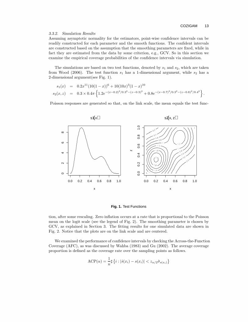
The simulations are based on two test functions, denoted by s1 and s2, which are takenfrom Wood (2006). The test function s1 has a 1-dimensional argument, while s2 has a2-dimensional argument(see Fig. 1).

s1(x) = 0.2x11(10(1 − x))6 + 10(10x)3(1 − x)10

s2(x, z) = 0.3 × 0.4π{

1.2e−(x−0.2)2/0.32−(z−0.3)2 + 0.8e−(x−0.7)2/0.32

−(z−0.8)2/0.42}

.

Poisson responses are generated so that, on the link scale, the mean equals the test func-

0.0 0.2 0.4 0.6 0.8 1.0

02

46

8

s1 (x)

x

s2 (x, z)

x

z

0.0 0.2 0.4 0.6 0.8 1.0

0.0

0.2

0.4

0.6

0.8

1.0

Fig. 1. Test Functions

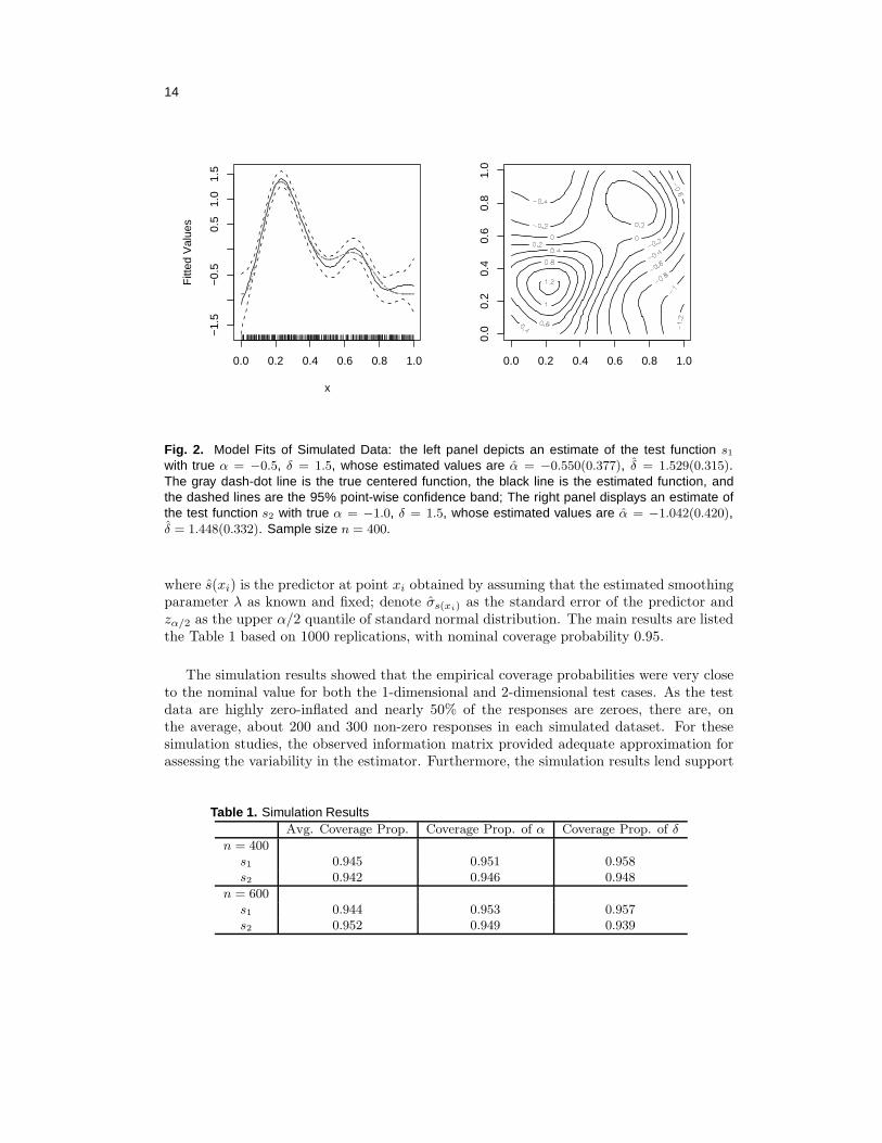
tion, after some rescaling. Zero inflation occurs at a rate that is proportional to the Poissonmean on the logit scale (see the legend of Fig. 2). The smoothing parameter is chosen byGCV, as explained in Section 3. The fitting results for one simulated data are shown inFig. 2. Notice that the plots are on the link scale and are centered.

We examined the performance of confidence intervals by checking the Across-the-FunctionCoverage (AFC), as was discussed by Wahba (1983) and Gu (2002). The average coverageproportion is defined as the coverage rate over the sampling points as follows.

ACP(α) =1

n♯{

i : |s(xi) − s(xi)| < zα/2σs(xi)

}

14

0.0 0.2 0.4 0.6 0.8 1.0

−1.

5−

0.5

0.5

1.0

1.5

x

Fitt

ed V

alue

s

0.0 0.2 0.4 0.6 0.8 1.0

0.0

0.2

0.4

0.6

0.8

1.0

Fig. 2. Model Fits of Simulated Data: the left panel depicts an estimate of the test function s1

with true α = −0.5, δ = 1.5, whose estimated values are α = −0.550(0.377), δ = 1.529(0.315).The gray dash-dot line is the true centered function, the black line is the estimated function, andthe dashed lines are the 95% point-wise confidence band; The right panel displays an estimate ofthe test function s2 with true α = −1.0, δ = 1.5, whose estimated values are α = −1.042(0.420),δ = 1.448(0.332). Sample size n = 400.

where s(xi) is the predictor at point xi obtained by assuming that the estimated smoothingparameter λ as known and fixed; denote σs(xi) as the standard error of the predictor andzα/2 as the upper α/2 quantile of standard normal distribution. The main results are listedthe Table 1 based on 1000 replications, with nominal coverage probability 0.95.

The simulation results showed that the empirical coverage probabilities were very closeto the nominal value for both the 1-dimensional and 2-dimensional test cases. As the testdata are highly zero-inflated and nearly 50% of the responses are zeroes, there are, onthe average, about 200 and 300 non-zero responses in each simulated dataset. For thesesimulation studies, the observed information matrix provided adequate approximation forassessing the variability in the estimator. Furthermore, the simulation results lend support

Table 1. Simulation ResultsAvg. Coverage Prop. Coverage Prop. of α Coverage Prop. of δ

n = 400s1 0.945 0.951 0.958s2 0.942 0.946 0.948

n = 600s1 0.944 0.953 0.957s2 0.952 0.949 0.939

COZIGAM 15

to the result thatE[ACP(α)] ≈ 1 − α,

see Wahba (1983).

4. Two Real Applications

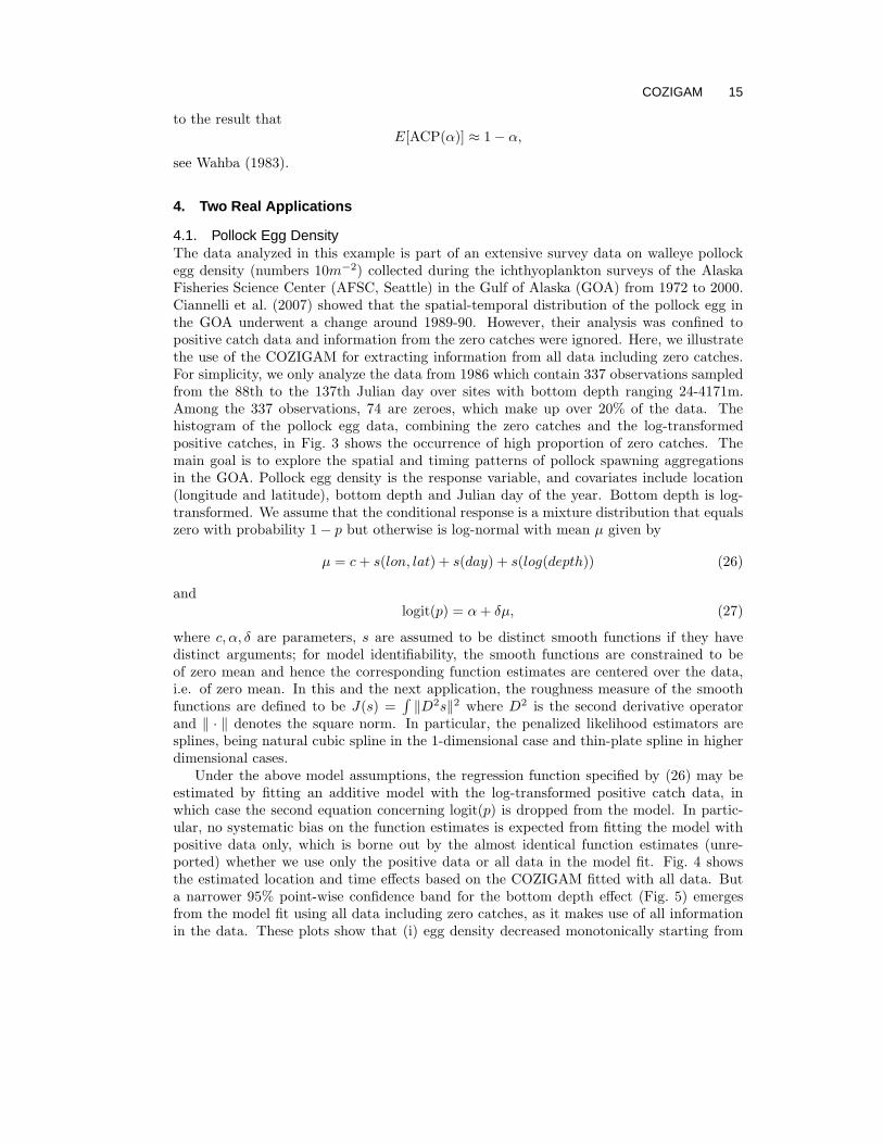
4.1. Pollock Egg DensityThe data analyzed in this example is part of an extensive survey data on walleye pollockegg density (numbers 10m−2) collected during the ichthyoplankton surveys of the AlaskaFisheries Science Center (AFSC, Seattle) in the Gulf of Alaska (GOA) from 1972 to 2000.Ciannelli et al. (2007) showed that the spatial-temporal distribution of the pollock egg inthe GOA underwent a change around 1989-90. However, their analysis was confined topositive catch data and information from the zero catches were ignored. Here, we illustratethe use of the COZIGAM for extracting information from all data including zero catches.For simplicity, we only analyze the data from 1986 which contain 337 observations sampledfrom the 88th to the 137th Julian day over sites with bottom depth ranging 24-4171m.Among the 337 observations, 74 are zeroes, which make up over 20% of the data. Thehistogram of the pollock egg data, combining the zero catches and the log-transformedpositive catches, in Fig. 3 shows the occurrence of high proportion of zero catches. Themain goal is to explore the spatial and timing patterns of pollock spawning aggregationsin the GOA. Pollock egg density is the response variable, and covariates include location(longitude and latitude), bottom depth and Julian day of the year. Bottom depth is log-transformed. We assume that the conditional response is a mixture distribution that equalszero with probability 1 − p but otherwise is log-normal with mean µ given by

µ = c+ s(lon, lat) + s(day) + s(log(depth)) (26)

andlogit(p) = α+ δµ, (27)

where c, α, δ are parameters, s are assumed to be distinct smooth functions if they havedistinct arguments; for model identifiability, the smooth functions are constrained to beof zero mean and hence the corresponding function estimates are centered over the data,i.e. of zero mean. In this and the next application, the roughness measure of the smoothfunctions are defined to be J(s) =

∫

‖D2s‖2 where D2 is the second derivative operatorand ‖ · ‖ denotes the square norm. In particular, the penalized likelihood estimators aresplines, being natural cubic spline in the 1-dimensional case and thin-plate spline in higherdimensional cases.

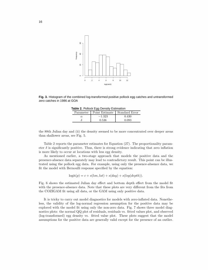
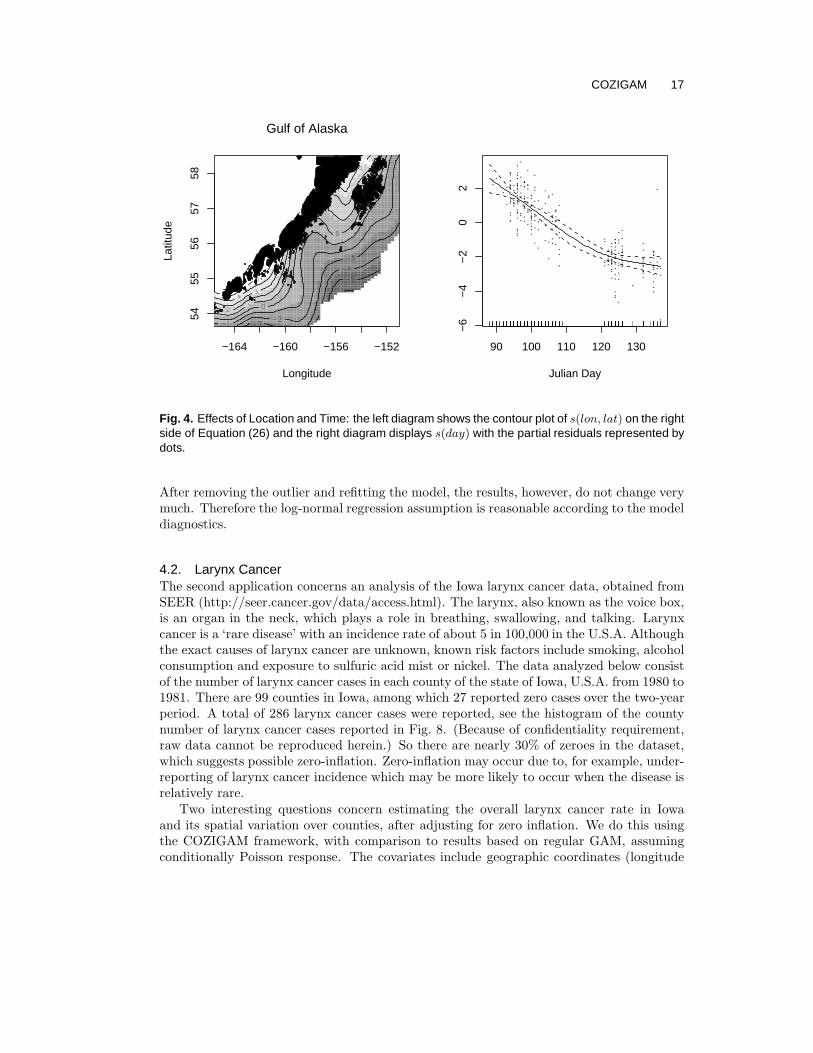
Under the above model assumptions, the regression function specified by (26) may beestimated by fitting an additive model with the log-transformed positive catch data, inwhich case the second equation concerning logit(p) is dropped from the model. In partic-ular, no systematic bias on the function estimates is expected from fitting the model withpositive data only, which is borne out by the almost identical function estimates (unre-ported) whether we use only the positive data or all data in the model fit. Fig. 4 showsthe estimated location and time effects based on the COZIGAM fitted with all data. Buta narrower 95% point-wise confidence band for the bottom depth effect (Fig. 5) emergesfrom the model fit using all data including zero catches, as it makes use of all informationin the data. These plots show that (i) egg density decreased monotonically starting from

16

log(catch)

Fre

quen

cy

0 2 4 6 8 10 120

2040

60

Fig. 3. Histogram of the combined log-transformed positive pollock egg catches and untransformedzero catches in 1986 at GOA

Table 2. Pollock Egg Density EstimationParameter Point Estimate Standard Error

α −1.323 0.430δ 0.536 0.093

the 88th Julian day and (ii) the density seemed to be more concentrated over deeper areasthan shallower areas, see Fig. 5.

Table 2 reports the parameter estimates for Equation (27). The proportionality param-eter δ is significantly positive. Thus, there is strong evidence indicating that zero inflationis more likely to occur at locations with less egg density.

As mentioned earlier, a two-stage approach that models the positive data and thepresence-absence data separately may lead to contradictory result. This point can be illus-trated using the pollock egg data. For example, using only the presence-absence data, wefit the model with Bernoulli response specified by the equation:

logit(p) = c+ s(lon, lat) + s(day) + s(log(depth)).

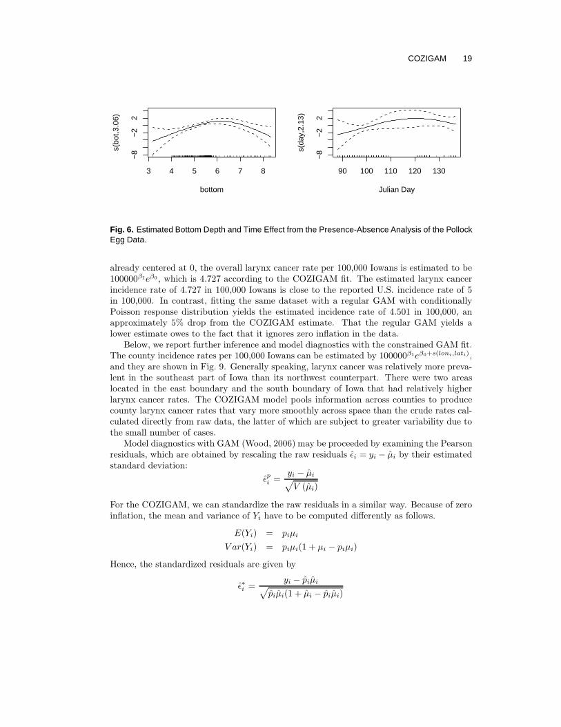
Fig. 6 shows the estimated Julian day effect and bottom depth effect from the model fitwith the presence-absence data. Note that these plots are very different from the fits fromthe COZIGAM fit using all data, or the GAM using only positive data.

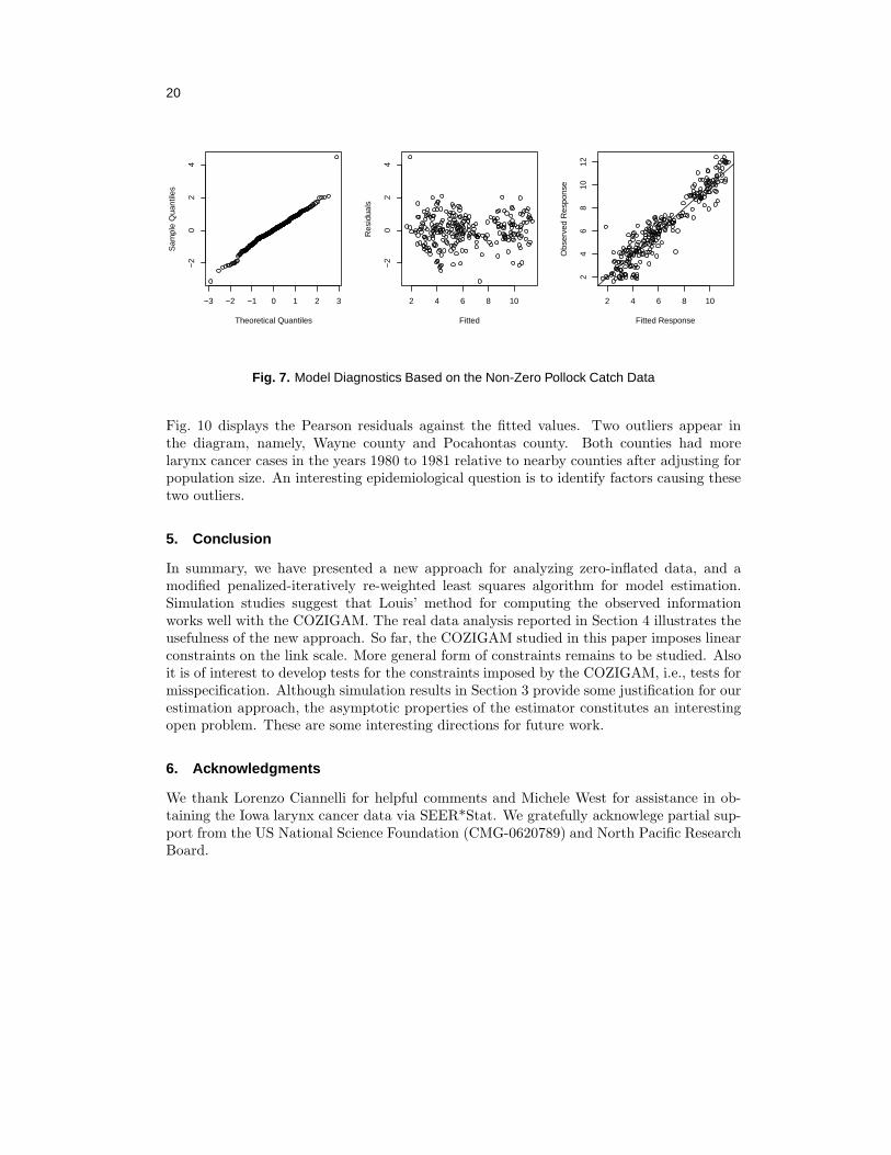
It is tricky to carry out model diagnostics for models with zero-inflated data. Nonethe-less, the validity of the log-normal regression assumption for the positive data may beexplored with the model fit using only the non-zero data. Fig. 7 shows three model diag-nostics plots: the normal QQ plot of residuals, residuals vs. fitted values plot, and observed(log-transformed) egg density vs. fitted value plot. These plots suggest that the modelassumptions for the positive data are generally valid except for the presence of an outlier.

COZIGAM 17

−164 −160 −156 −152

5455

5657

58

Gulf of Alaska

Longitude

Latit

ude

90 100 110 120 130

−6

−4

−2

02

Julian Day

Fig. 4. Effects of Location and Time: the left diagram shows the contour plot of s(lon, lat) on the rightside of Equation (26) and the right diagram displays s(day) with the partial residuals represented bydots.

After removing the outlier and refitting the model, the results, however, do not change verymuch. Therefore the log-normal regression assumption is reasonable according to the modeldiagnostics.

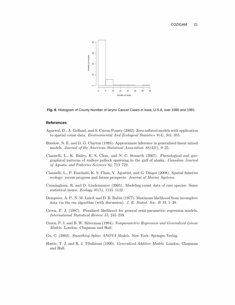
4.2. Larynx CancerThe second application concerns an analysis of the Iowa larynx cancer data, obtained fromSEER (http://seer.cancer.gov/data/access.html). The larynx, also known as the voice box,is an organ in the neck, which plays a role in breathing, swallowing, and talking. Larynxcancer is a ‘rare disease’ with an incidence rate of about 5 in 100,000 in the U.S.A. Althoughthe exact causes of larynx cancer are unknown, known risk factors include smoking, alcoholconsumption and exposure to sulfuric acid mist or nickel. The data analyzed below consistof the number of larynx cancer cases in each county of the state of Iowa, U.S.A. from 1980 to1981. There are 99 counties in Iowa, among which 27 reported zero cases over the two-yearperiod. A total of 286 larynx cancer cases were reported, see the histogram of the countynumber of larynx cancer cases reported in Fig. 8. (Because of confidentiality requirement,raw data cannot be reproduced herein.) So there are nearly 30% of zeroes in the dataset,which suggests possible zero-inflation. Zero-inflation may occur due to, for example, under-reporting of larynx cancer incidence which may be more likely to occur when the disease isrelatively rare.

Two interesting questions concern estimating the overall larynx cancer rate in Iowaand its spatial variation over counties, after adjusting for zero inflation. We do this usingthe COZIGAM framework, with comparison to results based on regular GAM, assumingconditionally Poisson response. The covariates include geographic coordinates (longitude

18

3 4 5 6 7 8

−8

−4

02

4

Bottom Depth

Fig. 5. Comparison of the COZIGAM (black) with the model using only the positive data (gray) onbottom depth effect; the dots represent the partial residuals from the COZIGAM.

Table 3. Iowa Larynx Cancer EstimationParameter Point Estimate Standard Error

β0 −9.098 0.754β1 0.925 0.065α 1.165 0.975δ 2.366 1.451

and latitude) and log-transformed county population size (sum of yearly population overthe study period). Specifically, the county numbers of larynx cancer cases constitute theresponse which is modeled to have a mixture distribution which for the ith county is zerowith probability 1−pi but otherwise a Poisson random variable with mean µi. The Poissonmean µi is a function of population, longitude and latitude:

log(µi) = β0 + s(log(popi)) + s(loni, lati)

where β0 is the intercept which is related to the overall incidence rate; s(log(popi)) ands(loni, lati) are two smooth functions that are centered, i.e., of zero mean, over the obser-vations. The probability pi is specified as

logit(pi) = α+ δ log(µi),

where α and δ are parameters. Preliminary analysis (unreported) suggests that the covariatelog(pop) affects the response linearly on the log scale, hence the model is simplified as follows:

log(µi) = β0 + β1 log(popi) + s(loni, lati)

The corresponding model estimation results are listed in Table 3.Note that the slope parameter δ is marginally significant, suggesting that zero inflation

occurs more frequently with lower incidence of the disease. Because the location effect is

COZIGAM 19

3 4 5 6 7 8

−8

−2

2

bottom

s(bo

t,3.0

6)

90 100 110 120 130

−8

−2

2

Julian Day

s(da

y,2.

13)

Fig. 6. Estimated Bottom Depth and Time Effect from the Presence-Absence Analysis of the PollockEgg Data.

already centered at 0, the overall larynx cancer rate per 100,000 Iowans is estimated to be100000β1eβ0 , which is 4.727 according to the COZIGAM fit. The estimated larynx cancerincidence rate of 4.727 in 100,000 Iowans is close to the reported U.S. incidence rate of 5in 100,000. In contrast, fitting the same dataset with a regular GAM with conditionallyPoisson response distribution yields the estimated incidence rate of 4.501 in 100,000, anapproximately 5% drop from the COZIGAM estimate. That the regular GAM yields alower estimate owes to the fact that it ignores zero inflation in the data.

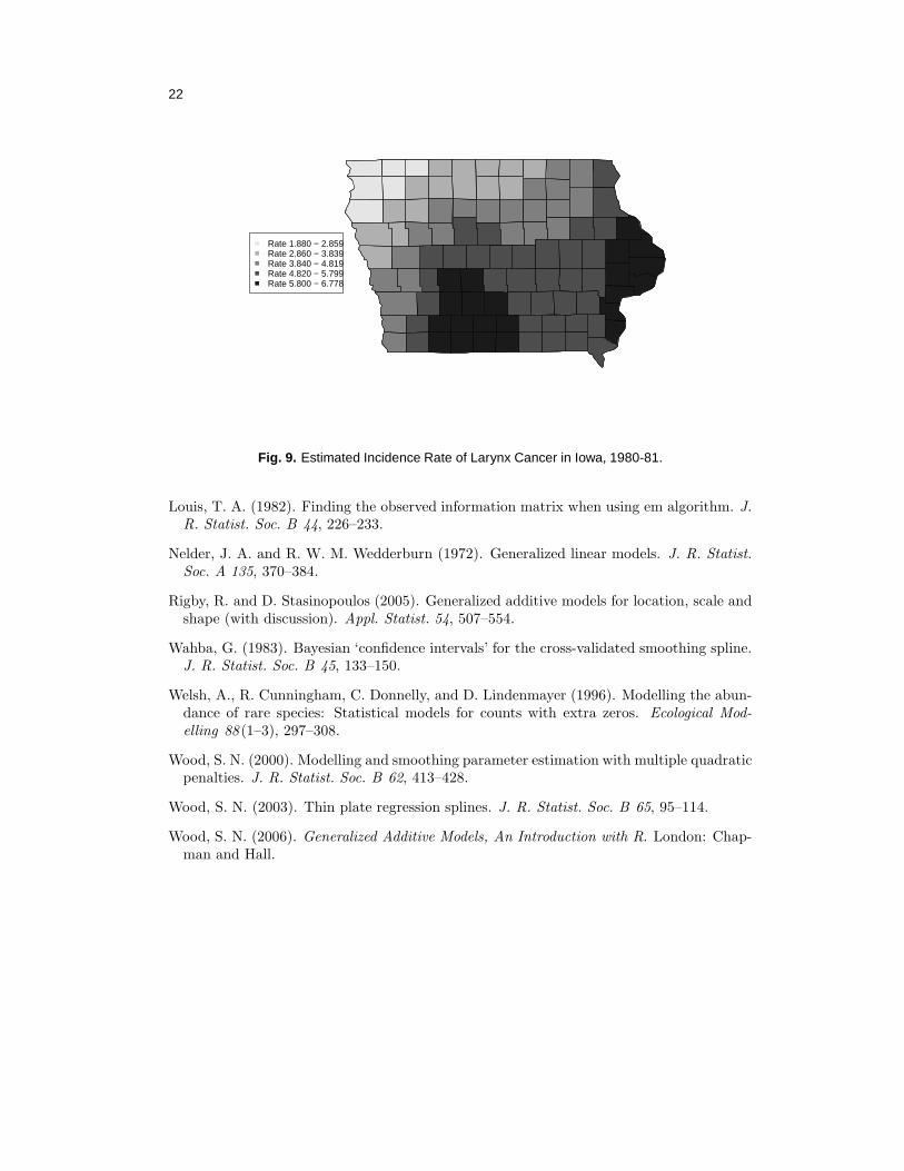
Below, we report further inference and model diagnostics with the constrained GAM fit.The county incidence rates per 100,000 Iowans can be estimated by 100000β1eβ0+s(loni,lati),and they are shown in Fig. 9. Generally speaking, larynx cancer was relatively more preva-lent in the southeast part of Iowa than its northwest counterpart. There were two areaslocated in the east boundary and the south boundary of Iowa that had relatively higherlarynx cancer rates. The COZIGAM model pools information across counties to producecounty larynx cancer rates that vary more smoothly across space than the crude rates cal-culated directly from raw data, the latter of which are subject to greater variability due tothe small number of cases.

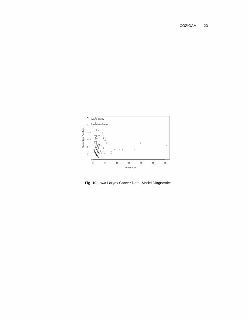
Model diagnostics with GAM (Wood, 2006) may be proceeded by examining the Pearsonresiduals, which are obtained by rescaling the raw residuals ǫi = yi − µi by their estimatedstandard deviation:

ǫpi =yi − µi√

V (µi)

For the COZIGAM, we can standardize the raw residuals in a similar way. Because of zeroinflation, the mean and variance of Yi have to be computed differently as follows.

E(Yi) = piµi

V ar(Yi) = piµi(1 + µi − piµi)

Hence, the standardized residuals are given by

ǫ∗i =yi − piµi

√

piµi(1 + µi − piµi)

20

−3 −2 −1 0 1 2 3

−2

02

4

Theoretical Quantiles

Sam

ple

Qua

ntile

s

2 4 6 8 10

−2

02

4

Fitted

Res

idua

ls

2 4 6 8 10

24

68

1012

Fitted Response

Obs

erve

d R

espo

nse

Fig. 7. Model Diagnostics Based on the Non-Zero Pollock Catch Data

Fig. 10 displays the Pearson residuals against the fitted values. Two outliers appear inthe diagram, namely, Wayne county and Pocahontas county. Both counties had morelarynx cancer cases in the years 1980 to 1981 relative to nearby counties after adjusting forpopulation size. An interesting epidemiological question is to identify factors causing thesetwo outliers.

5. Conclusion

In summary, we have presented a new approach for analyzing zero-inflated data, and amodified penalized-iteratively re-weighted least squares algorithm for model estimation.Simulation studies suggest that Louis’ method for computing the observed informationworks well with the COZIGAM. The real data analysis reported in Section 4 illustrates theusefulness of the new approach. So far, the COZIGAM studied in this paper imposes linearconstraints on the link scale. More general form of constraints remains to be studied. Alsoit is of interest to develop tests for the constraints imposed by the COZIGAM, i.e., tests formisspecification. Although simulation results in Section 3 provide some justification for ourestimation approach, the asymptotic properties of the estimator constitutes an interestingopen problem. These are some interesting directions for future work.

6. Acknowledgments

We thank Lorenzo Ciannelli for helpful comments and Michele West for assistance in ob-taining the Iowa larynx cancer data via SEER*Stat. We gratefully acknowlege partial sup-port from the US National Science Foundation (CMG-0620789) and North Pacific ResearchBoard.

COZIGAM 21

Number of cases

Num

ber

of c

ount

ies

0 5 10 15 20 25 30 350

2040

6080

Fig. 8. Histogram of County Number of larynx Cancer Cases in Iowa, U.S.A, over 1980 and 1981.

References

Agarwal, D., A. Gelfand, and S. Citron-Pousty (2002). Zero-inflated models with applicationto spatial count data. Environmental And Ecological Statistics 9 (4), 341–355.

Breslow, N. E. and D. G. Clayton (1993). Approximate inference in generalized linear mixedmodels. Journal of the American Statistical Association 88 (421), 9–25.

Ciannelli, L., K. Bailey, K. S. Chan, and N. C. Stenseth (2007). Phenological and geo-graphical patterns of walleye pollock spawning in the gulf of alaska. Canadian Journal

of Aquatic and Fisheries Sciences 64, 713–722.

Ciannelli, L., P. Fauchald, K. S. Chan, V. Agostini, and G. Dingsr (2008). Spatial fisheriesecology: recent progress and future prospects. Journal of Marine Systems.

Cunningham, R. and D. Lindenmayer (2005). Modeling count data of rare species: Somestatistical issues. Ecology 85 (5), 1135–1142.

Dempster, A. P., N. M. Laird, and D. B. Rubin (1977). Maximum likelihood from incompletedata via the em algorithm (with discussion). J. R. Statist. Soc. B 39, 1–38.

Green, P. J. (1987). Penalized likelihood for general semi-parametric regression models.International Statistical Review 55, 245–259.

Green, P. J. and B. W. Silverman (1994). Nonparametric Regression and Generalized Linear

Models. London: Chapman and Hall.

Gu, C. (2002). Smoothing Spline ANOVA Models. New York: Springer-Verlag.

Hastie, T. J. and R. J. Tibshirani (1990). Generalized Additive Models. London: Chapmanand Hall.

22

Rate 1.880 − 2.859Rate 2.860 − 3.839Rate 3.840 − 4.819Rate 4.820 − 5.799Rate 5.800 − 6.778

Fig. 9. Estimated Incidence Rate of Larynx Cancer in Iowa, 1980-81.

Louis, T. A. (1982). Finding the observed information matrix when using em algorithm. J.

R. Statist. Soc. B 44, 226–233.

Nelder, J. A. and R. W. M. Wedderburn (1972). Generalized linear models. J. R. Statist.

Soc. A 135, 370–384.

Rigby, R. and D. Stasinopoulos (2005). Generalized additive models for location, scale andshape (with discussion). Appl. Statist. 54, 507–554.

Wahba, G. (1983). Bayesian ‘confidence intervals’ for the cross-validated smoothing spline.J. R. Statist. Soc. B 45, 133–150.

Welsh, A., R. Cunningham, C. Donnelly, and D. Lindenmayer (1996). Modelling the abun-dance of rare species: Statistical models for counts with extra zeros. Ecological Mod-

elling 88 (1–3), 297–308.

Wood, S. N. (2000). Modelling and smoothing parameter estimation with multiple quadraticpenalties. J. R. Statist. Soc. B 62, 413–428.

Wood, S. N. (2003). Thin plate regression splines. J. R. Statist. Soc. B 65, 95–114.

Wood, S. N. (2006). Generalized Additive Models, An Introduction with R. London: Chap-man and Hall.

COZIGAM 23

0 5 10 15 20 25 30

−1

01

23

4

Fitted Values

Sta

ndar

dize

d R

esid

uals

Wayne County

Pocahontas County

Fig. 10. Iowa Larynx Cancer Data: Model Diagnostics