Embed Size (px)
Citation preview
© 2017 Royal Statistical Society 0035–9254/17/67000
Appl. Statist. (2017)
Generalized additive models with principalcomponent analysis: an application to time series ofrespiratory disease and air pollution data
Juliana B. de Souza,
Federal University of Espırito Santo, Vitoria, Brazil
Valderio A. Reisen,
Federal University of Espırito Santo, Vitoria, Brazil, and CentraleSupelec, Gif-sur-Yvette, France
Glaura C. Franco,
Federal University of Minas Gerais, Belo Horizonte, Brazil
Marton Ispany,
University of Debrecen, Hungary
Pascal Bondon
Centre National de la Recherche Scientifique and CentraleSupelec, Gif-sur-Yvette, and University of Paris–Saclay, France
and Jane Meri Santos
Federal University of Espırito Santo, Vitoria, Brazil
[Received March 2016. Revised July 2017]
Summary. Environmental epidemiological studies of the health effects of air pollution frequentlyutilize the generalized additive model (GAM) as the standard statistical methodology, consider-ing the ambient air pollutants as explanatory covariates. Although exposure to air pollutants ismulti-dimensional, the majority of these studies consider only a single pollutant as a covariatein the GAM model. This model restriction may be because the pollutant variables do not onlyhave serial dependence but also interdependence between themselves. In an attempt to con-vey a more realistic model, we propose here the hybrid generalized additive model–principalcomponent analysis–vector auto-regressive (GAM–PCA–VAR) model, which is a combinationof PCA and GAMs along with a VAR process. The PCA is used to eliminate the multicollinearitybetween the pollutants whereas the VAR model is used to handle the serial correlation of thedata to produce white noise processes as covariates in the GAM. Some theoretical and sim-ulation results of the methodology proposed are discussed, with special attention to the effectof time correlation of the covariates on the PCA and, consequently, on the estimates of theparameters in the GAM and on the relative risk, which is a commonly used statistical quantityto measure the effect of the covariates, especially the pollutants, on population health. As amain motivation to the methodology, a real data set is analysed with the aim of quantifying the
Address for correspondence: Marton Ispany, Faculty of Informatics, University of Debrecen, Debrecen, Kassaiut 26, 4028 Debrecen, Hungary.E-mail: [email protected]
2 J. B. de Souza, V. A. Reisen, G. C. Franco, M. Ispany, P. Bondon and J. Meri
association between respiratory disease and air pollution concentrations, especially particulatematter PM10, sulphur dioxide, nitrogen dioxide, carbon monoxide and ozone. The empiricalresults show that the GAM–PCA–VAR model can remove the auto-correlations from the principalcomponents. In addition, this method produces estimates of the relative risk, for each pollutant,which are not affected by the serial correlation in the data. This, in general, leads to morepronounced values of the estimated risk compared with the standard GAM model, indicating,for this study, an increase of almost 5.4% in the risk of PM10, which is one of the most importantpollutants which is usually associated with adverse effects on human health.
Keywords: Generalized additive model; Multicollinearity; Principal component analysis;Relative risk; Serial correlation; Vector auto-regressive model
1. Introduction
The effect of air pollutants on human wellbeing has motivated the study and control of atmo-spheric pollution, which affects human health even for low levels of air pollutants concentrationswithin air quality guidelines suggested by the World Health Organization (2006). Many studieshave found significant association between daily pollutant concentration levels and hospitaladmissions for respiratory and cardiovascular diseases; see Schwartz (2000), Ostro et al. (1999)and Chen et al. (2010), among others. The adverse effects of atmospheric pollutants on humanhealth are a source of concern to environmental and public health regulatory agencies. Popula-tion studies and epidemiological research have been used to identify these adverse health effectsand to guide the development of practices and legislation to control emissions and air quality.
The generalized additive model (GAM) with a Poisson marginal distribution has been themost widely applied method to measure and quantify the non-linear association between adversehealth effects and covariates such as ambient concentrations of air pollutants and meteorologicalconditions, mainly because it allows for non-parametric adjustments of non-linear confoundingeffects of seasonality and trends.
In spite of its widespread use, many researchers claim that care is needed when applying theGAM to time series. The fit can be affected, for instance, by a wrong choice of the number ofdegrees of freedom in the smooth component and by the presence of auto-correlation in theseries under study, among others (see for example, Dionisio et al. (2016)). Some works that aimto solve these problems include Dominici et al. (2002), who proposed a correction to the degreesof freedom in the smooth component, Dominici et al. (2006), Lall et al. (2011) and Michelozziet al. (2007), who have used lag-distributed models to relate the response variable to lagged valuesof a time-dependent predictor, and Figueiras et al. (2005) and Ramsey et al. (2003), who haveproposed some approaches to control the problem of concurvity (the non-linear dependence thatcan remain among the covariates). Additionally, most of the references in the epidemiologicalresearch area related to the study of the association between pollution and adverse health effectsusually consider only one pollutant whereas the population under study is exposed to a complexmixture of pollutants; a broad discussion of the effect of correlated measurement errors in timeseries on the relative risk estimates has recently been given in Dionisio et al. (2016). The choice ofa simple model may be, in general, due to the fact that the pollutants are linearly time-correlatedvariables, which implies bias in regression estimates since the presence of multicollinearity (thelinear dependence between the covariates) can inflate the variance of the estimators. This modelrestriction may not provide the true picture of the scenario in a real problem. As a result, thisincorrect analysis may lead to serious consequences on the health of the population under studysuch as a false positive conclusion of the pollution health risk.
One way to circumvent the problem of multicollinearity is to perform a principal com-ponent analysis (PCA) on the pollutants covariance matrix. PCA is a multivariate statisti-cal technique and it is generally used to reduce the dimensionality of a set of data while
Generalized Additive Models with Principal Component Analysis 3
preserving, as much as possible, the variability in the covariates; see Johnson and Wichern(2007). Evaluating the adverse health effects of a combination of pollutants may be easier tointerpret and more feasible than isolating the effects of a single pollutant. Some researchershave explored this relevant research direction. For example, Roberts and Martin (2006) evalu-ated how the pollutants PM10, ozone .O3/, sulphur dioxide .SO2/, nitrogen dioxide .NO2/ andcarbon monoxide (CO) affect health, where the issue of multicollinearity was handled by usingPCA. Roberts and Martin (2006) also developed a PCA supervised method in which the rela-tionship between the covariates (the pollutants) and deleterious health effects are determinedbefore the covariates are inserted into the regression model. Recently, Wang and Pham (2011)studied the combined effects of pollutants on daily mortality by using PCA and a robust method.The relative risk estimates RR of the results were more significant when the multivariate PCAtechnique was used. Nevertheless, application of the PCA technique generally requires the datato be obtained through independent replications. All the time series that are considered in thispaper are supposed to be stationary (including the covariates). As the principal components(PCs) are linear combinations of the covariates, their properties are linearly transferred to thePCs. Therefore, the use of PCA to perform statistical inferences on time-correlated covariates,such as ambient concentration of atmospheric pollutants, should be further examined.
Zamprogno (2013) has addressed this issue by using theoretical and empirical methods todetermine the effect of neglecting the time correlation of the covariates in the PCA technique.Zamprogno (2013) showed that the PCs are auto-correlated if the covariates are also auto-correlated. The PCs contain the time structure of the covariates and must therefore be usedjudiciously in the regression analysis. To remove the temporal correlation structures of PCA,Zamprogno (2013) suggested filtering the series by using a multivariate auto-regressive movingaverage model in the pollution variables before performing any statistical analysis using PCA.In the same context, Matteson and Tsay (2011) and Hua and Tsay (2014) applied vector auto-regressive (VAR) models to remove the serial correlation of time series of stock returns beforecarrying out PCA on the residuals of the VAR model. The use of Box–Jenkins methodology toeliminate the serial correlation in the data was also considered in Campbell (1994) who discussedthe relationship between sudden infant death syndrome with environmental temperature byusing time regression for counts with Poisson marginal distribution.
In the current study, the multicollinearity issue is solved by using PCA on the pollutants,with the components obtained being used as covariates in the GAM. This procedure is calledGAM–PCA. Additionally, the problem that is associated with the presence of auto-correlationin the PCs when applying the GAM is circumvented by using a VAR model on the time seriesof covariates before obtaining the PCs. This new model is called here GAM–PCA–VAR. Thesetwo models are formulated theoretically as probabilistic latent variable models in Section 2.The GAM–PCA and GAM–PCA–VAR models are compared with the conventional GAM bymeans of adequate goodness-of-fit statistics and, also, in terms of the relative risk estimate RR,which is a commonly used tool to measure the effect of the covariates, especially the pollutants,on population health. Some results that are related to the methods proposed and the effect ofauto-correlated covariates on the PCA are theoretically and empirically discussed. In addition,the estimate of the relative risk RR is evaluated for each model in a real data problem. Theobjective of estimating RR is to verify whether there is any change in this statistic due to thecharacteristics of the covariates under study, such as temporal correlation, among others. As amain result of this paper, we find that the two procedures (GAM–PCA and GAM–PCA–VAR)evidenced larger relative risk estimates than those obtained by using a conventional GAM. Asimulation study demonstrates that the intercorrelation and auto-correlation that are found inthe explanatory pollutant variables may be responsible for this divergence. This is important
4 J. B. de Souza, V. A. Reisen, G. C. Franco, M. Ispany, P. Bondon and J. Meri
evidence that prevents use of the standard GAM, from the epidemiological point of view, sincethe time series phenomena in the explanatory pollutant variables can produce unrealistic riskimpacts on the health of the population under study, i.e. this may indicate a false positive result.
The paper is organized as follows. Section 2 presents the statistical models that are addressedhere, such as GAMs, PCA and VAR models, in detail. Section 3 discusses some simulationsresults and the analysis of a real data set. Section 4 concludes the work.
The data that are analysed in the paper and the programs that were used to analyse them canbe obtained from
http://wileyonlinelibrary.com/journal/rss-datasets
2. Methodology: generalized additive models, principal component analysis,vector auto-regressive models and relative risk
In this section, we present the methodology that is employed to relate the covariates to thecount time series under study. As there are both linear and non-linear relationships between theexplanatory variables and the response, a GAM model is used. The procedures are implementedby using count data with a Poisson distribution, as this is a very useful model in practicalsituations.
We also present, in detail, the PCA and VAR methodologies, to explain how these proceduresare linked to solve problems that can occur with the kind of data that we are working with, whichmeans multicollinearity and serial correlation in the explanatory variables.
2.1. Generalized additive modelsThe GAM (see Hastie and Tibshirani (1990)) with a Poisson marginal distribution is typicallyused to relate a discrete outcome variable with a set of covariates in the epidemiological area, forexample, to quantify the association between health problems and air pollution concentrations.The GAM is widely used to describe non-linear correlations between the variables of interest;see, for example, Schwartz (2000), Ostro et al. (1999) and Chen et al. (2010).
Let {Yt}≡ {Yt}t∈Z be a count time series, i.e. it is composed of non-negative integer-valuedrandom variables. The conditional distribution of Yt , given the past Ft−1 which contains theavailable information up to time t − 1, is characterized by the weights p.yt|Ft−1/ := P.Yt =yt|Ft−1/ where yt ∈{0, 1, : : :}. If Yt has a conditional Poisson distribution with mean μt , then
p.yt ;μt|Ft−1/= exp.−μt/μytt
yt !, yt =0, 1, : : : :
Thus, the conditional log-likelihood function of the mutually conditionally independent randomvariables Y1, : : : , Yn is given by
l.μ/ :=n∑
t=1ln{p.Yt ;μt|Ft−1/}∝
n∑t=1
{Yt ln.μt/−μt}, .1/
where the vector μ := .μ1, : : : , μq/T depends on the covariates and the parameters of the process{Yt}. Let Xt = .X1t , : : : , Xpt/
T be the vector of covariates of dimension p at time t, where ‘T’denotes the transpose, which may include past values of Yt and other auxiliary variables, such asthe pollutants and confounding variables (i.e. trends, seasonality and meteorological variables,among others). In what follows, X1t , : : : , Xqt denote the pollutants, whereas X.q+1/t , : : : , Xpt
denote the confounding variables at time t (q�p).
Generalized Additive Models with Principal Component Analysis 5
The relationship between Yt and the vector Xt of covariates is obtained by setting (see, forexample, Kedem and Fokianos (2002))
ln.μt/=q∑
j=0βjXjt +
p∑j=q+1
fj.Xjt/, q�p,
where .β0, β/ with β := .β1, : : : , βq/T is the vector of the coefficients to be estimated (βj is thecoefficient of the jth covariate), and fj is a smoothing function of an appropriate function spacefor the jth confounding variable (e.g. the temperature or the humidity variables). Moreover, β0denotes the curve intercept and is associated with X0t =1 for all t. For simplicity it is assumedthat the pollutant covariates are centred. The aforementioned model is usually referred to asa semiparametric model because it involves parametric and non-parametric functions. Theparameters of the parametric functions are generally estimated by using maximum likelihoodor quasi-likelihood methods, by optimizing the log-likelihood defined in expression (1), with theasymptotic properties given in Kedem and Fokianos (2002). The non-parametric functions areevaluated by using ‘splines’, ‘LOESS’ or moving average functions, among others (see Friedman(1991) and Wahba (2001)).
The relative risk RR is frequently used in epidemiological studies to measure the effect of at-mospheric pollutant concentrations on the health of the exposed population. RR for a pollutantcovariate Xj, j =1, : : : , q, is defined as the relative change in the expected count of respiratorydisease events per ξ-unit change in the covariate while keeping the other covariates fixed. Moreprecisely, see formula (8) in Baxter et al. (1997):
RRXj .ξ/ := E.Y |Xj = ξ, Xi =xi, i �= j/
E.Y |Xj =0, Xi =xi, i �= j/:
For Poisson regression RR does not depend on the values xi, i �= j, of the other covariates andit can be expressed as
RRXj .ξ/= exp.βjξ/:
RR is often called the relative rate or rate ratio; see, for example, page 265 in Dalgaard (2008).Note that for binary outcomes RR is defined as the ratio of probabilities that an event will occurfollowing a certain exposure or non-exposure to a risk factor; see Zou (2004). RR can also beinterpreted in this study as the ratio of probabilities that a patient is suffering from respiratorydiseases per ξ-unit change in a pollutant covariate. RR and its approximate confidence intervalat an α level of significance of a covariate Xj, j = 1, : : : , q, in the GAM with Poisson marginaldistribution are estimated as follows:
RRXj .ξ/= exp.βjξ/,
CI{RRXj .ξ/}= exp{βjξ ∓ zα=2 se.βj/ξ},
where ξ is the variation in the pollutant concentration (e.g. a value of 10μg m−3 of interquartilevariation), βj is the estimated coefficient for the pollutant Xj being studied with standard errorse.βj/ and zα=2 denotes the .1−α=2/-quantile of the standard normal distribution. At an α levelof significance, the hypothesis to be tested is defined as H0 :RRXj =1 against H1 :RRXj >1 whereRRXj :=RRXj .1/, i.e. RR for a unit change in Xj. The rejection of H0 statistically implies thatthe pollutant has a significant adverse health effect.
2.2. Principal component analysisPCA is a multivariate statistical technique that aims, in general, to reduce the dimensionality
6 J. B. de Souza, V. A. Reisen, G. C. Franco, M. Ispany, P. Bondon and J. Meri
of a data matrix space through linear transformations of the original variables. The correlationbetween the variables implies the occurrence of multicollinearity in the regression models. In thisstudy, the PCA technique is used to circumvent the problem of pollutants that are correlatedwith each other. In general, the whole variability of a system determined by q variables can onlybe explained by using all the q PCs. However, a large part of this variability can be explainedby using a lower number r of components (r �q); see Johnson and Wichern (2007).
Consider the following pairs of eigenvalues and eigenvectors of the covariance matrix ΣX ofthe random vector X = .X1, : : : , Xq/T : .λ1, a1/, .λ2, a2/, : : : , .λq, aq/, where λ1 � λ2 � : : : � λq.The ith PC of ΣX is
Zi =aTi X =a1iX1 +a2iX2 + : : :+aqiXq, .2/
i=1, 2, : : : , q, with the properties
var.Zi/=aTi ΣXai =λi,
cov.Zi, Zj/=aTi ΣXaj =0,
i, j =1, 2, : : : , q, i �= j, since the eigenvectors are orthogonal.For a stationary vector time series {Xt} ≡ {Xt}t∈Z, Xt = .X1t , : : : , Xqt/
T, with covariancematrix ΣX, the PCs are defined as Zit =aT
i Xt , i=1, : : : , q, and
cov.Zit , Zjt/=aTi cov.Xt , Xt/aj =aT
i ΓX.0/aj ={
λi if i= j,0 otherwise,
.3/
and
cov.Zit , Zj.t+h//=aTi cov.Xt , Xt+h/aj =aT
i ΓX.h/aj, .4/
where ΓX.h/ denotes the autocovariance matrix function of {Xt} at lag h with ΓX.0/=ΣX. Thisresult is proved in Zamprogno (2013).
Equation (3) shows that at zero lag the PCs are uncorrelated whereas equation (4) demon-strates that PCA preserves the auto-correlation structures in time-correlated covariates, i.e., forall i=1, : : : , q, Zi ≡{Zit}t∈Z is a time series and the auto-correlation of Zi, ρZi.h/ �=0, h=±1,: : : , provided that the eigenvector ai is not in the null space of the autocovariance matricesΓX.h/, h �=0, which holds clearly, for example, if these matrices have full rank. In addition, Zi
and Zj, j �= i, are cross-correlated, i.e. ρZi,Zj .h/ �=0 for all h=±1, ±2 : : : :
Thus, PCA must be used judiciously in time series regression models. We propose in Section2.4 an alternative method to eliminate the auto-correlation of the PCs.
2.3. Generalized additive modelling and principal component analysisOne of the research directions that is developed in this paper is the combined use of the PCAtechnique and a GAM, which is denoted here as GAM–PCA. This hybrid method was previouslyconsidered in Wang and Pham (2011) without taking into account the temporal effect in themodel parameter estimates. Note that this model is also referred to as a PCA-based GAM(see Zhao et al. (2014)), where the model is applied to quantify the relationships between fishpopulations and their environment.
In the GAM–PCA model the covariates Z1t , : : : , Zqt that are generated by the PCA are linearcombinations of the original variables X1t , : : : , Xqt . Mathematically, Zit = aT
i Xt , similarly toequation (2), but the PCs are now time dependent for all i=1, : : : , q. These new covariates areused in the GAM. Let r � q and, considering the first r pairs of eigenvalues and eigenvectorsof the covariance matrix ΣX, define the matrices Λr := diag.λ1, : : : , λr/ and Ar := .a1, : : : , ar/,
Generalized Additive Models with Principal Component Analysis 7
i.e. the eigenvectors form columns of matrix Ar. We can see that Ar is an orthogonal matrixof dimension q × r, i.e. AT
r Ar = Ir where Ir is an identity matrix of dimension r. Moreover,AT
r ΣXAr =Λr. Let Λ=Λq and A=Aq. Then Λr is the top left-hand block of Λ of size r × r andAr consists of the first r columns of A; see, for example, page 11 in Jolliffe (2002). Any linearcombination of the first r new covariates can be expressed as a linear combination of the originalcovariates in the following way:
r∑i=1
υiZit =q∑
j=1
r∑i=1
υiajiXjt =q∑
j=1βÅ
j Xjt , .5/
where υ := .υ1, : : : , υr/T and βÅ := .βÅ
1 , : : : , βÅq /T are vectors of dimensions r and q respectively,
and the relationship between vectors υ and βÅ is given by βÅ =Arυ and thus υ=ATr βÅ, i.e., in
the GAM–PCA model, the new parameter vector βÅ of the original covariates is in the rangeof matrix Ar. Then, the link function of the GAM–PCA model using the first r PCs is given as
μt.υ0, υ, A/= exp{
r∑i=0
υiZit +p∑
j=q+1fj.Xjt/
}
= exp{
υ0 +υTATr Xt +
p∑j=q+1
fj.Xjt/
}.6/
with r � q � p, where Xt := .X1t , : : : , Xqt/T is the vector of covariates, υ0 corresponds to the
curve intercept with Z0t =1 for all t, υ is the vector of coefficients of the first r PCs and fjs arethe smoothing functions for the confounding variables (i.e. the temperature and the humidityin this study). In the definition of the link function we denote only the parameters of the newPC covariates and the transformation matrix of the PCA.
The GAM–PCA model can be considered as a probabilistic latent variable model defined by
Yt|Ft−1 ∼Po.μt/,
Xt =AZt
with link function (6), where Po.·/ denotes the Poisson distribution, the latent variables {Zt}form a vector white noise process of dimension q with diagonal variance matrix Λ (see definition11.1.2 in Brockwell and Davis (1991)) and A is an orthogonal matrix of dimension q ×q. Thequadruple .υ0, υ, A, Λ/ forms the parameters of the GAM–PCA model to be estimated. Clearly,the latent variables can be expressed as Zt = ATXt for all t. Hence, GAM–PCA can also beinterpreted as a two-stage model where, in the first stage, new variables (PCs) are derived by thePCA using the original covariates and, in the second stage, a GAM is fitted by using these newvariables. If {Zt} and thus {Xt} are Gaussian processes then the joint distribution of .Yt , Xt/
can be expressed as a product of a Poisson and a Gaussian distribution. Thus, given a sample.X1, Y1/, : : : , .Xn, Yn/, the log-likelihood, up to a constant, is derived as a hybrid sum of a Poissonand a Gaussian log-likelihood:
l.υ0, υ, A, Λ/∝n∑
t=1{Yt ln.μt/−μt}− 1
2
n∑t=1
.ATXt/TΛ−1.ATXt/− n
2ln{det.Λ/}, .7/
where μt depends on the parameters by the link function (6). The parameters of the GAM–PCA model can be estimated, for example, by the maximum likelihood method. Since thelog-likelihood (7) is quite complicated the maximization with respect to its parameters is morecomplex; hence a two-stage method is proposed. Firstly, the parameter matrices A and Λ areestimated by applying the PCA to the estimated covariance matrix ΣX. Secondly, the parametersυ0 and υ are estimated by fitting the GAM with link function (6) using the first r PCs. Note that
8 J. B. de Souza, V. A. Reisen, G. C. Franco, M. Ispany, P. Bondon and J. Meri
this procedure works without assuming any distribution assumption for the covariates. In thecase of Gaussian covariates the maximization of the Gaussian part of the log-likelihood (7) isequivalent to the application of PCA to these covariates. In what follows, the assumption of anormal distribution for covariates is used only in computing the standard information criteriafor model selection. The approach that was discussed above is similar to PC regression (see, forexample, chapter 8 in Jolliffe (2002)), and it can be considered as a two-stage regression method,which is a procedure that is well known in the econometric area; see Amemiya (1985).
In this context, the estimate of RR per ξ-unit change in the pollutant concentration for theoriginal covariate Xj, j =1, : : : , q, is
RRÅXj
.ξ/= exp.βÅj ξ/, .8/
where ξ is, for example, the interquartile variation. The term βÅj is given by
βÅj :=
r∑i=1
ajiυi, j =1, : : : , q, .9/
where υi is the estimated coefficient of the ith PC in equation (6) and ai, i=1, : : : , r, are the firstr estimated eigenvectors. Equation (9) can be easily derived by using equation (5). Since the PCsare uncorrelated the standard error of β
Åj can be estimated by
se2.βÅj /=
r∑i=1
a2ji se2.υi/:
2.4. Generalized additive modelling, principal component analysis and vector auto-regressive modellingAs previously discussed, the use of PCA for time series produces auto-correlations and cross-correlations between the PCs. In this paper, we suggest a procedure to eliminate the auto-correlations and cross-correlations of these components by applying a vector auto-regressivemoving average (VARMA) filter to the original data to obtain a white noise process; see, also,Greenaway-McGrevy et al. (2012). The model proposed, called here GAM–PCA–VAR, aimsto eliminate the temporal correlation to obtain estimates of the regression parameters, andconsequently RR-estimates, which are free from the serial correlation in the covariates thatcould lead to spurious analysis in real applications.
Let now {Xt}, Xt = .X1t , X2t : : : , Xqt/T, be a VARMA.pÅ, qÅ/ process defined as the solution
to the following system (see Hamilton (1994)):
Φ.B/.Xt −γ/=Θ.B/εt , .10/
where B is the delay operator, γ is a q-dimensional vector and the innovation process {εt}is q-dimensional white noise with E.εt/ = 0 and var.εt/ = Σε, where Σε is a q × q variancematrix. The operators Φ.B/= Iq −ΣpÅ
i=1ΦiBi and Θ.B/= Iq+ΣqÅ
i=1ΘiBi are polynomial matrices
of orders pÅ and qÅ respectively, and the Φis and Θis are matrices of constants with dimensionq × q. If det{Φ.z/} �= 0 for all complex z such that |z| � 1 then the VARMA model (10) hasexactly one stationary solution; see theorem 11.3.1 in Brockwell and Davis (1991). SeasonalVARMA models are built by using the same structure as in equation (10), but with the lag timebeing a multiple of the seasonal period.
The VAR(1) model is a particular case of the VARMA.pÅ, qÅ/ model with pÅ =1 and qÅ =0.Without loss of generality, it is here assumed that γ =0. Therefore, model (10) simplifies to
Xt =ΦXt−1 +εt : .11/
Generalized Additive Models with Principal Component Analysis 9
A VAR(1) process has a unique stationary solution provided that all the eigenvalues of Φ areless than 1 in absolute value. In this case, the unique solution of the VAR(1) model can beexpressed as the almost surely convergent infinite series Xt =Σ∞
j=0Φjεt−j; see example 11.3.1 in
Brockwell and Davis (1991). The autocovariance matrix function of {Xt} is given by ΓX.h/=Σ∞
j=0Φj+hΣε.ΦT/j, h=0, ±1, : : :. The identification and estimation procedures for model (10)
are given in Hamilton (1994) and Brockwell and Davis (1991). The seasonal VAR(1) modelwith period s, which is usually denoted by SVARs.1/, is an extension of model (11) with aseasonal matrix auto-regressive coefficient at lag s. This seasonal matrix must satisfy a similarstationary condition to that of the VAR(1) model; see, for example, Brockwell and Davis (1991).In what follows, the model proposed here, which combines PCA, VAR and GAM procedures,is discussed.
The GAM–PCA–VAR model is a combination of the VAR(1) model (11), where Xt representsthe pollution variables at time t in the context of this paper, and the GAM–PCA model by usingthe white noise error process (11) as covariates. Mathematically, let Z1t , : : : , Zqt at time t begiven by
Zit =aTi εt =aT
i .Xt −ΦXt−1/, i=1, : : : , q, .12/
where .λi, ai/, i = 1, : : : , q, denote the first r eigenvalues and eigenvectors of the variance ma-trix Σε of the white noise innovation in equation (11), and, therefore, the PC vector Zt hasnow uncorrelated components Zi ≡ {Zit}, i = 1, : : : , q, and these components are white noiseprocesses with variances λi, i=1, : : : , q, respectively. The effect of the VAR(1) filter in the GAM–PCA–VAR model is to eliminate the serial correlation in the original pollutant covariates. Largepositive values in a co-ordinate of the innovation εt indicate locally high environmental influ-ence according to this pollutant at time t. In contrast, large negative values indicate negligibleinfluence. The GAM–PCA–VAR model that is based on the first r PCs is defined by
μt.υ0, υ, A, Φ/= exp{
r∑i=0
υiZit +p∑
j=q+1fj.Xjt/
}
= exp{
υ0 +υTATr Xt −υTAT
r ΦXt−1 +p∑
j=q+1fj.Xjt/
}, .13/
which clearly shows that, in contrast with GAM–PCA, Yt depends on both Xt and Xt−1, demon-strating the presence of serial dependence in the GAM–PCA–VAR model.
The GAM–PCA–VAR model can also be considered as a probabilistic latent variable modeldefined by
Yt|Ft−1 ∼Po.μt/,
Xt =ΦXt−1 +AZt
with link function (13), where the latent variables {Zt} form a vector white noise process ofdimension q with diagonal variance matrix Λ, A is an orthogonal matrix of dimension q×q andΦ is a matrix of dimension q × q. The quintuplet .υ0, υ, A, Λ, Φ/ forms the parameters of theGAM–PCA–VAR model to be estimated. Clearly, the latent variable can be expressed as Zt =AT.Xt −ΦXt−1/ for all t; see also equation (12). Hence, GAM–PCA–VAR can be interpreted asa three-stage model, where in the first stage the temporal dependence is eliminated by taking thenew serially uncorrelated variable εt =Xt −ΦXt−1 at time t; in the second stage new uncorrelatedvariables (PCs) {Zt} are derived by using the PCA for the innovation process {εt}, and in thethird stage a GAM is fitted by using the first r PCs as covariates. The order of models in the
10 J. B. de Souza, V. A. Reisen, G. C. Franco, M. Ispany, P. Bondon and J. Meri
term GAM–PCA–VAR corresponds to these stages starting with the third and finishing withthe first, which is generally accepted in the time series literature.
Under the assumption that the distribution of the innovation vector is multivariate normal, theconditional log-likelihood of the GAM–PCA–VAR model, given a sample .X1, Y1/, : : : , .Xn, Yn/,is derived as
l.υ0, υ, A, Λ, Φ/∝n∑
t=2{Yt ln.μt/−μt}− 1
2
n∑t=2
.Xt −ΦXt−1/TAΛ−1AT.Xt −ΦXt−1/
− n−12
ln{det.Λ/}, .14/
where μt depends on the parameters by the link function (13). Since maximization of this log-likelihood is also quite computationally expensive, a three-stage estimation method is proposed:firstly, a VAR(1) model is fitted to the original covariates by applying standard time seriestechniques; secondly, using PCA for the residuals defined by "t =Xt − ΦXt−1, t =2, : : : , n, whereΦ denotes the estimated auto-regressive coefficient matrix in the fitted VAR(1) model, the first r
PCs are computed; thirdly, a GAM model is fitted using these PCs by maximizing the Poissonpart of log-likelihood (14). The relative risk of the GAM–PCA–VAR model, which is computedsimilarly to expression (8), is denoted here by RR
ÅÅ.
Remark 1. Another model, called hereafter GAM–VAR–PCA, can be derived by interchang-ing the order of the VAR filter and PCA. Namely, the multicollinearity between the originalcovariates is eliminated by PCA firstly and then the serial dependence is handled by VAR mod-elling. More precisely, let Ar be defined as in Section 2.3 and Z.r/
t =ATr Xt for all t. We fit a VAR(1)
model to the r-dimensional process {Z.r/t }, i.e. Z.r/
t =ΨrZ.r/t−1 + W.r/
t , where Ψr is a matrix ofdimension r × r and {W.r/
t }, W.r/t = .W
.r/1t , : : : , W
.r/rt /T, is an r-dimensional white noise process.
The link function of the GAM–VAR–PCA model is
μt.υ0, υ, Ar, Ψr/= exp{
r∑i=0
υiW.r/it +
p∑j=q+1
fj.Xjt/
}
= exp{
υ0 +υTATr Xt −υTΨrA
Tr Xt−1 +
p∑j=q+1
fj.Xjt/
}, .15/
which looks like equation (13). Nevertheless, there is an important difference between thesetwo formulations. Whereas, in the GAM–PCA–VAR model, the vector Z.r/
t = .Z1t , : : : , Zrt/T
in equation (13) is a white noise process with uncorrelated components Zi ≡{Zit}, i=1, : : : , r,in the GAM–VAR–PCA model, the vector W.r/
t in equation (15) is also a white noise processbut its components are not necessarily uncorrelated. Hence, the new covariates of the GAM–VAR–PCA model that are involved in the GAM model are no longer uncorrelated and, thus,the estimators of its parameters may present bias and high variance. For this reason, the GAM–VAR–PCA model is not a correct alternative.
2.5. Goodness of fitA comparison of the procedures proposed is performed by means of some goodness-of-fitstatistics, such as the mean-square error MSE, Akaike information criterion AIC and Bayesianinformation criterion BIC. The estimated MSE is defined as
MSE= 1n
n∑i=1
.Yi − Y i/2,
where Y i is the predicted value of Yi, the number of hospital treatments. The Akaike information
Generalized Additive Models with Principal Component Analysis 11
criterion AIC (see Akaike (1973)) and the Bayesian information criterion BIC (see Schwarz(1978)), which are widely applied for model selection, are defined as
AIC=−2l+2k,
BIC=−2l+k ln.n/,
where l is the maximized value of the log-likelihood function defined by expressions (1), (7) and(14) for the GAM, GAM–PCA and GAM–PCA–VAR models respectively, k is the number offree parameters to be estimated and n is the sample size. Note that k=1+ r.q+2/− r.r+1/=2 forGAM–PCA and k=1+ r.q+2/+q2 − r.r +1/=2 for GAM–PCA–VAR models since the degreeof freedom in q× r orthogonal real matrices is rq− r.r +1/=2. In this study, the log-likelihood l
is evaluated at the parameter values resulting from the proposed two- and three-stage estimationmethods for GAM–PCA and GAM–PCA–VAR models respectively.
3. Results
3.1. Simulation studyTo evaluate the effect in the parameter estimation, and hence in the RR-estimates, of a GAM inthe presence of temporal correlation in both the dependent Yt and independent Xt = .X1t , : : : ,Xqt/
T vector, a simple simulation study was conducted. The data were generated under threescenarios: independent data (scenario 1); the dependent variable is a time series and the covari-ates are independent random vectors in time (scenario 2); both the dependent and independentvariables are time series (scenario 3). For the three scenarios, the data were generated from aconditional Poisson model, Yt|Xt ∼Po.μt/.
Initially, only one covariate X1 was considered. In this case, for (scenario 1), the predictor isgiven by log.μt/ =β0 +β1X1t where X1t ∼ N.0, 1/ for all t, which means that neither {Yt} nor{X1t} are time series. Under scenarios 2 and 3, the predictor is given by log.μt/=β0 +β1X1t +εt ,where {εt} ∼ AR.1/ with auto-regressive coefficient ϕ = 0:1, 0:5, 0:9. The difference betweenscenarios 2 and 3 is that, for the first, X1t ∼N.0, 1/ for all t and, for the latter, {X1t}∼ AR.1/
with φ= 0:5. Thus, scenario 2 represents the case where {Yt} is a time series, but {X1t} is notand scenario 3 represents the case where both {Yt} and {X1t} are time series. For these threescenarios, β0 =1, β1 =1:5, the sample size is n=100 and the number of Monte Carlo simulationswas equal to 1000. The empirical values of the mean, bias and MSE are displayed in Table 1.All results were obtained by using R code.
In the case of independent data (scenario 1), the estimate of β1 is very close to the true value,as expected. However, the picture changes dramatically especially in scenario 3. It can be seenthat the estimate of β1 is heavily affected by the auto-correlation structure in the data, by pre-senting a negative bias which increases in absolute value as ϕ increases positively. Hence, theestimated MSE also increases substantially with ϕ. In particular, for the last scenario whenboth {Yt} and {X1t} are time series, it can be seen that the fitted GAM tends to underesti-mate β1 severely. As RR is a function of β1, its bias also introduces bias in the RR-estimatesin the sense that it tends to decrease when the auto-correlation structure increases. Hence,the correlation structure in the data may attenuate the true RR-estimate, which can lead to afalse positive conclusion (this empirical evidence was also discussed in Dionisio et al. (2016)in a different simulation scenario). Thus, if a GAM is fitted to time series variables, withoutmitigating the temporal correlation structure of the covariates as, for example, by removingthis from the data, the RR-estimate may not correspond to the true relationship between thevariables.
Next, we evaluate the effect in the parameter estimation of a GAM when there are two
12 J. B. de Souza, V. A. Reisen, G. C. Franco, M. Ispany, P. Bondon and J. Meri
Table 1. Simulation results for a single covariate
Scenario Parameter Mean Bias MSE
1, independent β0 =1 0.9958 −0.0042 0.0049β1 =1:5 1.5010 0.0010 0.0026
2, ϕ=0:1 β0 =1 1.4873 0.4873 0.2921β1 =1:5 1.4457 −0:0543 0.0671
2, ϕ=0:5 β0 =1 1.6084 0.6084 0.4782β1 =1:5 1.4091 −0.0909 0.1116
2, ϕ=0:9 β0 =1 2.7779 1.7779 4.7168β1 =1:5 1.3189 −0.1811 0.2544
3, ϕ=0:1 β0 =1 1.4732 0.4732 0.3673β1 =1:5 1.3903 −0:1097 0.1180
3, ϕ=0:5 β0 =1 1.6512 0.6512 0.5727β1 =1:5 1.3790 −0.1210 0.1528
3, ϕ=0:9 β0 =1 2.8475 1.8475 5.0797β1 =1:5 1.2518 −0.2482 0.2918
Table 2. Simulation results for two covariates X1 and X2
Scenario Parameter Mean Bias MSE
1, independent β0 =1 0.9964 −0:0036 0.0048β1 =1:5 1.5015 0.0015 0.0026β2 =0:5 0.4999 −0:0001 0.0020
2 β0 =1 1.5955 0.5955 0.5180β1 =1:5 1.4799 −0:0201 0.0701β2 =0:5 0.4719 −0:0281 0.0621
3, φ11 =0:7, φ12 =0, β0 =1 1.6254 0.6254 0.7941φ21 =0, φ22 =0:5 β1 =1:5 1.3708 −1:1292 0.1208
β2 =0:5 0.4596 −0:0404 0.07013, φ11 =0:7, φ12 =0:4, β0 =1 1.6654 0.6654 1.3042
φ21 =0, φ22 =0:5 β1 =1:5 1.3559 −0:1441 0.1299β2 =0:5 0.4487 −0:0513 0.0933
covariates, Xt = .X1t , X2t/T. The set-up is the same as described previously for scenarios 1,
2 and 3, with two covariates instead of a single one. Thus, under scenario 1 the predictoris given by log.μt/ = β0 + β1X1t + β2X2t , where X1t , X2t ∼ N.0, 1/ are independent for all t.Under scenarios 2 and 3, the predictor is given by log.μt/ = β0 + β1X1t + β2X2t + εt , where{εt}∼ AR.1/, with ϕ= 0:5. Now the difference between scenarios 2 and 3 is that, for the first,X1t , X2t ∼ N.0, 1/, mutually independent, and, for the latter, .X1t , X2t/
T forms a VAR(1) pro-cess with auto-regressive coefficient matrix Φ of dimension 2 × 2. The results are displayed inTable 2.
From Table 2, similar conclusions are drawn to those in the case of a single covariate (Table1), i.e. the coefficients of X1 and X2 are always underestimated when the process is generatedby time series, either in the response or in the covariate vector. Nevertheless, the bias in theestimates is much larger in a more complex model structure compared with the case of a singlecovariate.
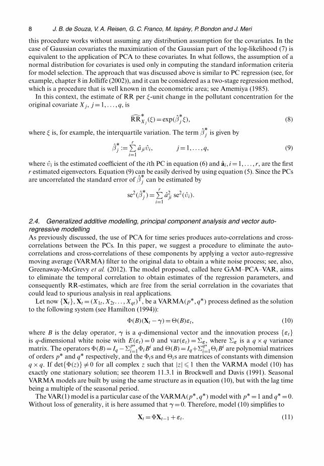
The next empirical study has the aim to illustrate, with a simple simulated model, the timecorrelation effect in the PCA as discussed in Section 2.2, more specifically, the result of equation
Generalized Additive Models with Principal Component Analysis 13
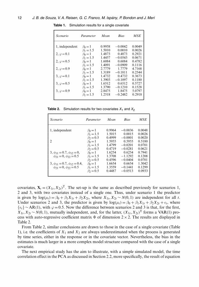
Fig. 1. Sample auto-correlation function and cross-correlation function of the PCs: (a) PC 1; (b) PC 1�PC 2;(c) PC 2�PC 1; (d) PC 2
(4). For this one sample {X1, : : : , X500} was generated from the process {Xt} in equation (11)that follows a two-dimensional VAR(1) model with φ11 =φ22 =0:5, φ12 =0:1 and φ21 =0:8 andGaussian white noise vector with
Σε =(
1 0:30:3 1
):
The estimated PCs, i.e. Z1t , Z2t , t =1, : : : , 500, were computed from the 2×2 sample covariancematrix of {X1, : : : , X500}. The sample correlation and cross-correlation functions of the PCsare displayed in Fig. 1, in which Z1t and Z2t correspond to PC 1 and PC 2 respectively. Ascan be seen, the plots clearly indicate that the correlation structure of the models is transferredto the PCs as shown in equation (4). On the basis of the above empirical evidence as well ason the discussion of the previous sections, it is clear that the temporal correlation cannot beneglected when using PCA in regression models with covariates being time series data; other-wise the conclusions can be totally erroneous and lead to severe consequences. Therefore, theuse of the proposed methodology discussed in Section 2.4 can be an alternative approach tomitigate this problem. These issues are also discussed in the next section, but with a real dataset.
3.2. Data analysisIn this study, the number of daily hospital admissions for respiratory diseases was obtainedfrom the main childrens’ emergency department in the Vitoria metropolitan area (called theHospital Infantil Nossa Senhora da Gloria). Respiratory diseases are classified according to
14 J. B. de Souza, V. A. Reisen, G. C. Franco, M. Ispany, P. Bondon and J. Meri
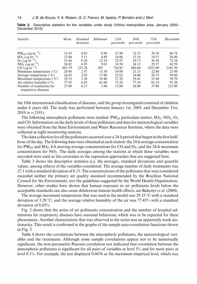
Table 3. Descriptive statistics for the variables under study (Vitoria metropolitan area, January 2005–December 2010)
Statistic Mean Standard Minimum 25th 50th 75th Maximumdeviation percentile percentile percentile
PM10 .μg m−3/ 33.45 8.83 8.98 27.90 32.75 38.39 86.74SO2 .μg m−3/ 12.44 3.11 4.89 10.06 12.16 14.57 26.48O3 .μg m−3/ 31.86 8.36 12.10 25.97 30.73 36.58 72.34NO2 .μg m−3/ 24.82 6.93 9.03 19.59 24.13 29.37 62.59CO .μg m−3/ 885.79 231.28 295 724.82 866.60 1031.09 2141.50Minimum temperature .◦C/ 20.86 2.47 13.10 19.08 21.15 22.80 25.98Average temperature .◦C/ 24.43 2.45 17.00 22.62 24.40 26.35 30.80Maximum temperature .◦C/ 29.35 3.28 19.40 27.20 29.41 31.60 39.70Air relative humidity (%) 77.43 6.03 61.60 73.24 77.19 81.14 97.28Number of treatments for 27.09 6.15 1.00 13.00 24.00 37.00 121.00
respiratory diseases
the 10th international classification of diseases, and the group investigated consisted of childrenunder 6 years old. The study was performed between January 1st, 2005, and December 31st,2010 .n=2191/.
The following atmospheric pollutants were studied: PM10 particulate matter, SO2, NO2, O3and CO. Information on the daily levels of these pollutants and data for meteorological variableswere obtained from the State Environment and Water Resources Institute, where the data werecollected at eight monitoring stations.
The data collection for all the pollutants occurred over a 24-h period that began in the first half-hour of the day. The following data were obtained at each station: the 24-h average concentrationfor PM10 and SO2, 8-h moving average concentrations for CO and O3, and the 24-h maximumconcentration for NO2. The daily averages among the stations at which these variables wererecorded were used as the covariates in the regression approaches that are suggested here.
Table 3 shows the descriptive statistics (i.e. the averages, standard deviations and quantilevalues, among others) of the variables considered. The average number of daily treatments was27.1 with a standard deviation of 6.15. The concentrations of the pollutants that were consideredexceeded neither the primary air quality standard recommended by the Brazilian NationalCouncil for the Environment, nor the guidelines suggested by the World Health Organization.However, other studies have shown that human exposure to air pollutants levels below theacceptable standards can also cause deleterious human health effects; see Bakonyi et al. (2004).
The average maximum temperature that was used in the model was 29:35 ◦C with a standarddeviation of 3:28 ◦C, and the average relative humidity of the air was 77.43% with a standarddeviation of 6.03%.
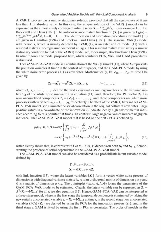
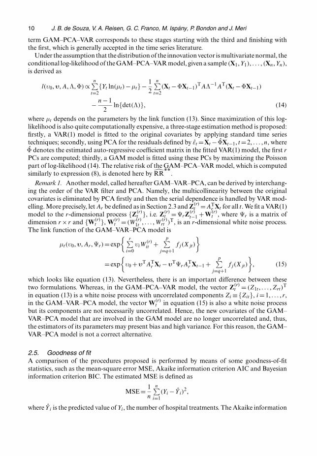
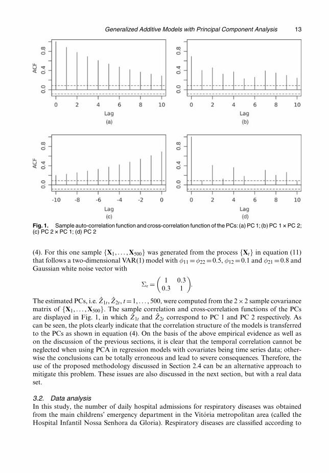
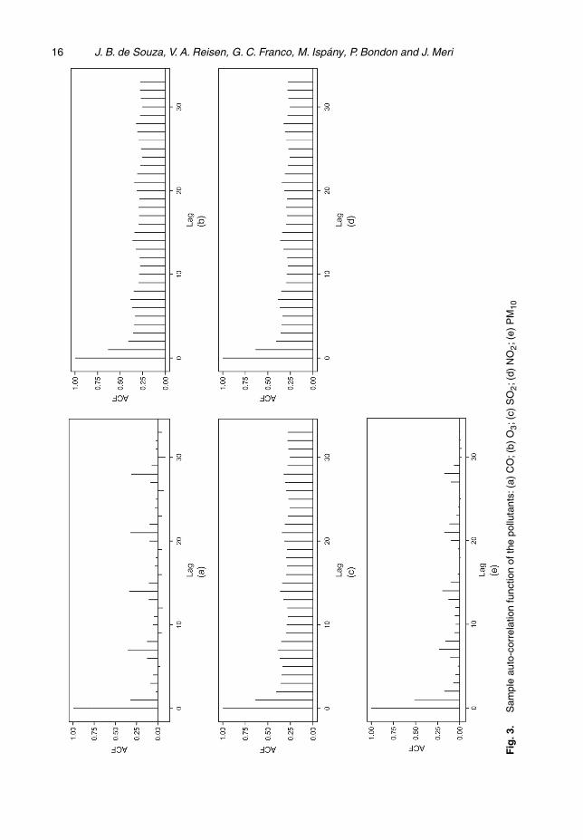
Fig. 2 shows that the series of air pollutants concentration and the number of hospital ad-missions for respiratory diseases have seasonal behaviour, which was to be expected for thesephenomena. Another characteristic that was observed in the series was an apparently weak sta-tionarity. This result is confirmed in the graphs of the sample auto-correlation functions shownin Fig. 3.
Table 4 shows the correlations between the atmospheric pollutants, the meteorological vari-ables and the treatments. Although some sample correlations appear not to be numericallysignificant, the non-parametric Pearson correlation test indicated that correlation between theatmospheric pollutants is significant for all pairs of variables at level 5% and for most pairs atlevel 0.1%. For example, the test displayed 0.0476 as the maximum empirical level, which was
Generalized Additive Models with Principal Component Analysis 15
Fig
.2.
Con
cent
ratio
nof
(a)
CO
,(b)
NO
2,(
c)S
O2,(
d)P
M10
and
(e)
O3,a
nd(f
)nu
mbe
rof
trea
tmen
tsfo
rre
spira
tory
dise
ases
16 J. B. de Souza, V. A. Reisen, G. C. Franco, M. Ispany, P. Bondon and J. Meri
Fig
.3.
Sam
ple
auto
-cor
rela
tion
func
tion
ofth
epo
lluta
nts:
(a)
CO
;(b)
O3;(
c)S
O2;(
d)N
O2;(
e)P
M10
Generalized Additive Models with Principal Component Analysis 17
Table 4. Correlation between pollutants, meteorological variables and number of treatments†
PM10 SO2 NO2 CO O3 T (max) T (min) RH Number oftreatments
PM10 1.00SO2 0.31 1.00NO2 0.34 0.04 1.00CO 0.35 0.22 0.61 1.00O3 −0:04 −0:08 0.04 −0:40 1.00T (max) 0.20 0.44 −0:43 −0:06 −0:23 1.00T (min) −0:10 0.16 −0:48 −0:10 −0:16 0.62 1.00RH −0:28 −0:29 0.23 0.26 −0:22 −0:44 −0:03 1.00Number of 0.05 −0:33 0.09 0.09 −0:08 −0:15 −0:19 0.14 1.00
treatments
†T, temperature .◦C/; RH, air relative humidity (%); all correlations were significant at a 5% level.
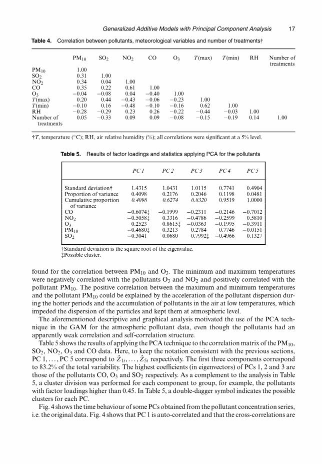
Table 5. Results of factor loadings and statistics applying PCA for the pollutants
PC 1 PC 2 PC 3 PC 4 PC 5
Standard deviation† 1.4315 1.0431 1.0115 0.7741 0.4904Proportion of variance 0.4098 0.2176 0.2046 0.1198 0.0481Cumulative proportion 0.4098 0.6274 0.8320 0.9519 1.0000
of varianceCO −0:6074‡ −0:1999 −0:2311 −0:2146 −0:7012NO2 −0:5058‡ 0.3316 −0:4786 −0:2599 0.5810O3 0.2523 0.8615‡ −0:0363 −0:1995 −0:3911PM10 −0:4680‡ 0.3213 0.2784 0.7746 −0:0151SO2 −0:3041 0.0680 0.7992‡ −0:4966 0.1327
†Standard deviation is the square root of the eigenvalue.‡Possible cluster.
found for the correlation between PM10 and O3. The minimum and maximum temperatureswere negatively correlated with the pollutants O3 and NO2 and positively correlated with thepollutant PM10. The positive correlation between the maximum and minimum temperaturesand the pollutant PM10 could be explained by the acceleration of the pollutant dispersion dur-ing the hotter periods and the accumulation of pollutants in the air at low temperatures, whichimpeded the dispersion of the particles and kept them at atmospheric level.
The aforementioned descriptive and graphical analysis motivated the use of the PCA tech-nique in the GAM for the atmospheric pollutant data, even though the pollutants had anapparently weak correlation and self-correlation structure.
Table 5 shows the results of applying the PCA technique to the correlation matrix of the PM10,SO2, NO2, O3 and CO data. Here, to keep the notation consistent with the previous sections,PC 1, : : : , PC 5 correspond to Z1t , : : : , Z5t respectively. The first three components correspondto 83.2% of the total variability. The highest coefficients (in eigenvectors) of PCs 1, 2 and 3 arethose of the pollutants CO, O3 and SO2 respectively. As a complement to the analysis in Table5, a cluster division was performed for each component to group, for example, the pollutantswith factor loadings higher than 0.45. In Table 5, a double-dagger symbol indicates the possibleclusters for each PC.
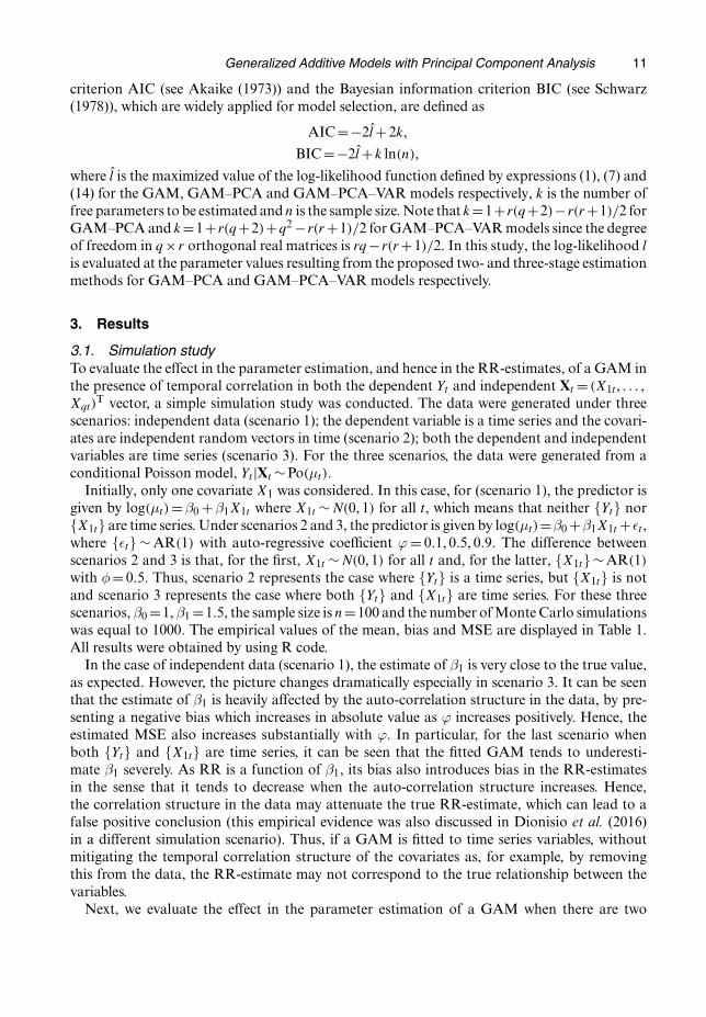
Fig. 4 shows the time behaviour of some PCs obtained from the pollutant concentration series,i.e. the original data. Fig. 4 shows that PC 1 is auto-correlated and that the cross-correlations are
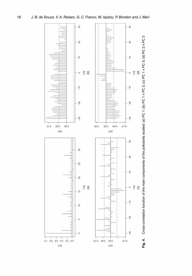
18 J. B. de Souza, V. A. Reisen, G. C. Franco, M. Ispany, P. Bondon and J. Meri
Fig
.4.
Cro
ss-c
orre
latio
nfu
nctio
nof
the
mai
nco
mpo
nent
sof
the
pollu
tant
sst
udie
d:(a
)P
C1;
(b)
PC
1�P
C2;
(c)
PC
1�P
C3;
(d)
PC
2�P
C3
Generalized Additive Models with Principal Component Analysis 19
Fig
.5.
(a)
Sam
ple
auto
-cor
rela
tion
func
tion
and
(b)
sam
ple
part
iala
uto-
corr
elat
ion
func
tion
ofth
ere
sidu
als
ofth
eG
AM
–PC
Am
odel
20 J. B. de Souza, V. A. Reisen, G. C. Franco, M. Ispany, P. Bondon and J. Meri
Table 6. Results of the final GAM–PCA model to estimate the effects ofpollutants concentrations on hospital admissions in the Vitoria metropolitanarea
Variable† Estimate Standard error Z-value p-value
(Intercept) 4.4871 0.0901 49.82 0.0000‡Tuesday −0:1596 0.0152 −10:50 0.0000‡Wednesday −0:2176 0.0154 −14:14 0.0000‡Thursday −0:1321 0.0151 −8:76 0.0000‡Friday −0:1571 0.0154 −10:22 0.0000‡Saturday −0:1204 0.0150 −8:04 0.0000‡Sunday −0:0860 0.0154 −5:59 0.0000‡Holiday 2 0.1886 0.0440 4.29 0.0000‡Holiday 3 0.3189 0.0384 8.30 0.0000‡Air relative humidity −0:0061 0.0009 −6:83 0.0000‡PC 1 −0:0244 0.0040 −6:16 0.0000‡PC 2 0.0163 0.0055 2.99 0.0028§PC 3 −0:0157 0.0056 −2:79 0.0052‡
†Holiday 2, Corpus Christ plus Our Lady of Penha; holiday 3, carnival plusholiday (Tiradentes day) plus Brazil’s Independence day.‡Significant at the 0.001 level.§Significant at the 0.01 level.
non-null, corroborating the results that were discussed in Sections 2.2 and 3.1. The componentsalso clearly exhibited the seasonal behaviour of the pollution variables, as expected, i.e. thegraphs show that the auto-correlation structure of the pollutants persists in the components.Therefore, the PCA technique should be applied carefully even for processes with an apparentlyweak auto-correlation structure. This is an argument contrary to page 299 in Jolliffe (2002), inwhich the author argues that
‘when the main objective of PCA is only descriptive, complications such as non-independence (temporal)does not seriously affect this objective’
(see, also, Zamprogno (2013) and Vanhatalo and Kulachi (2016)).The cumulative proportion of the variance was the choice criterion for the components to
be included in the GAM. Thus, following the parsimony criterion, the first three componentswere chosen as covariates (highlighted in italics in Table 5), which corresponds to 83.2% of thetotal variability and the simplest model as possible to handle the complex correlation structureof the data. The number of daily treatments for respiratory diseases was considered to be thedependent variable, and each outcome was modelled on the basis of the assumption that thecount of respiratory disease events (i.e. hospital admissions) followed a conditional Poissondistribution.
The analysis involved several procedures implemented in stages. Initially, the short-term sea-sonality was treated by using indicator variables for week days and holidays. A LOESS smooth-ing function (see Friedman (1991)) was used to model the long-term seasonality to control forthe non-linear dependence. The confounding covariates (i.e. the temperature and the relativehumidity) were modelled by using spline smoothing curves (see Friedman (1991) and Wahba(2001)). The best GAM–PCA fit was obtained on the basis of a residual analysis and the Akaikeinformation criterion AIC (Akaike, 1973).
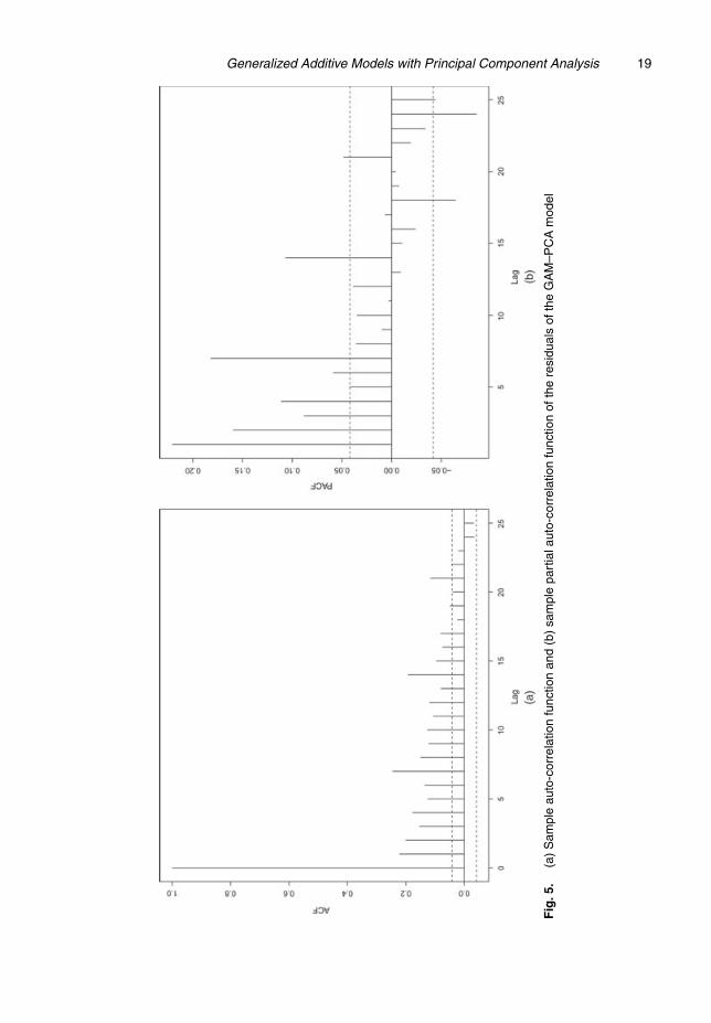
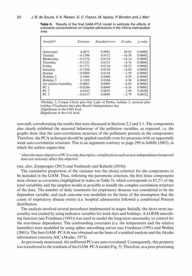
As previously mentioned, the unfiltered PCs are auto-correlated. Consequently, this propertywas transferred to the residuals of the GAM–PCA model (Fig. 5). Therefore, as a post-processing
Generalized Additive Models with Principal Component Analysis 21
Fig
.6.
(a)
Sam
ple
auto
-cor
rela
tion
func
tion
and
(b)
part
iala
uto-
corr
elat
ion
func
tion
ofth
ere
sidu
als
ofth
efin
alG
AM
–PC
Am
odel
22 J. B. de Souza, V. A. Reisen, G. C. Franco, M. Ispany, P. Bondon and J. Meri
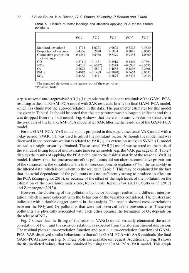
Table 7. Results of factor loadings and statistics applying PCA for the filteredpollutants
PC 1 PC 2 PC 3 PC 4 PC 5
Standard deviation† 1.4774 1.0223 0.9628 0.7228 0.5680Proportion of variance 0.4366 0.2090 0.1854 0.1045 0.0645Cumulative proportion 0.4366 0.6456 0.8310 0.9355 1.0000
of varianceCO 0.5711‡ −0:1431 0.2918 −0:1469 0.7393NO2 0.4205 −0:6527‡ 0.2543 −0:0905 −0:5695O3 −0:3693 −0:5801‡ −0:4685 −0:4896 0.2606PM10 0.4012 −0:1409 −0:7040‡ 0.5663 0.0532SO2 0.4468 0.4441 −0:3675 −0:6402 −0:2414
†The standard deviation is the square root of the eigenvalue.‡Possible cluster.
step, a seasonal auto-regressive SAR.1/.1/7, model was fitted to the residuals of the GAM–PCA,resulting in the final GAM–PCA model with SAR residuals, briefly the final GAM–PCA model,which has eliminated the auto-correlation in the data. The parameter estimates for this modelare given in Table 6. It should be noted that the temperature was no longer significant and thuswas dropped from the final model. Fig. 6 shows that there is no auto-correlation structure inthe residuals of the final GAM–PCA model after SAR filtering the residuals of the GAM–PCAmodel.
For the GAM–PCA–VAR model that is proposed in this paper, a seasonal VAR model with a7-day period, SVAR7.1/, was used to adjust the pollutant vector. Although the model that wasdiscussed in the previous section is related to VAR(1), its extension using an SVAR7.1/ modelinstead is straightforwardly obtained. The seasonal VAR(1) model was selected on the basis ofthe standard fitting tools of multivariate time series models, e.g. the VAR package of R. Table 7displays the results of applying the PCA technique to the residual matrix of the seasonal VAR(1)model. It shows that the time structure of the pollutants did not alter the cumulative proportionof the variance, i.e. the variability in the first three components explains 83% of the variability inthe filtered data, which is equivalent to the results in Table 5. This may be explained by the factthat the serial dependence of the pollutants was not sufficiently strong to produce an effect onthe PCA (Zamprogno, 2013), or because of the effect of the high levels of the pollutant on theestimation of the covariance matrix (see, for example, Reisen et al. (2017), Cotta et al. (2017)and Zamprogno (2013)).
However, the clustering of the pollutants by factor loadings resulted in a different interpre-tation, which is more coherent with the behaviour of the variables considered. The clusters areindicated with a double-dagger symbol in the analysis. The results showed cross-correlationsbetween the NO2 and O3 pollutants that were not observed in the previous case. These twopollutants are physically associated with each other because the formation of O3 depends onthe release of NO2.
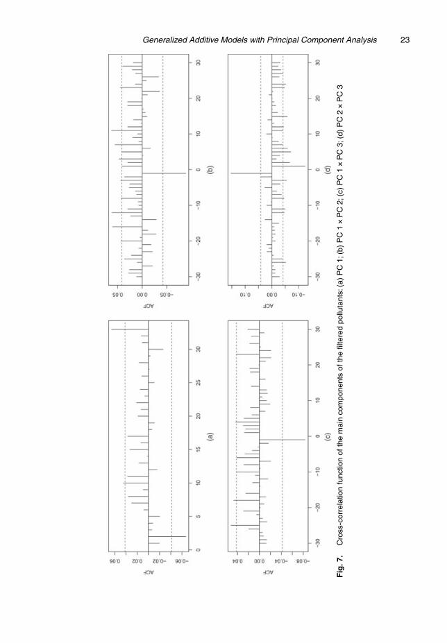
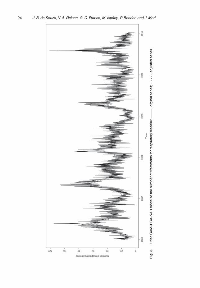
Fig. 7 shows that the fitting of the seasonal VAR(1) model virtually eliminated the auto-correlation of PC 1 and the cross-correlation, as expected from the aforementioned discussion.The residual plots (auto-correlation function and partial auto-correlation function) of GAM–PCA–VAR displayed similar behaviour to that of the GAM–PCA with SAR residuals (the finalGAM–PCA) shown in Fig. 6. These plots are available on request. Additionally, Fig. 8 showsthe fit (predicted values) that was obtained by using the GAM–PCA–VAR model. This graph
Generalized Additive Models with Principal Component Analysis 23
Fig
.7.
Cro
ss-c
orre
latio
nfu
nctio
nof
the
mai
nco
mpo
nent
sof
the
filte
red
pollu
tant
s:(a
)P
C1;
(b)
PC
1�P
C2;
(c)
PC
1�P
C3;
(d)
PC
2�P
C3
24 J. B. de Souza, V. A. Reisen, G. C. Franco, M. Ispany, P. Bondon and J. Meri
Fig
.8.
Fitt
edG
AM
–PC
A–V
AR
mod
elto
the
num
ber
oftr
eatm
ents
for
resp
irato
rydi
seas
e:,o
rgin
alse
ries;
,adj
uste
dse
ries
Generalized Additive Models with Principal Component Analysis 25
Table 8. Goodness-of-fit statistics for the estimatedmodels
Model MSE AIC BIC
GAM 1.480 24610 24720GAM–PCA 1.143 24442 24245GAM–PCA–VAR 1.144 24166 24190
Table 9. Relative risk RR and 95% confidence intervals for treatments forrespiratory diseases in children under 6 years old for an interquartile variationin the pollutants PM10, SO2, NO2, O3 and CO in the Vitoria metropolitan areafrom January 2005 to December 2010†
Pollutant RR RRÅ
RRÅÅ
PM10 1.020 (1.010,1.039) 1.029 (1.001,1.090) 1.075 (1.001,1.092)SO2 1.040 (1.010,1.080) 0.982 (0.972,1.001) 1.027 (1.010,1.040)CO 1.020 (1.010,1.030) 1.048 (1.002,1.071) 1.077 (1.020,1.100)NO2 1.000 (0.990,1.020) 1.028 (1.010,1.040) 1.012 (1.010,1.030)O3 0.980 (0.972,1.001) 1.081 (1.003,1.093) 0.992 (0.992,1.020)
†RR, GAM; RRÅ, GAM–PCA; RRÅÅ, GAM–PCA–VAR.
shows that the model provided a good fit to the data for the variable of interest, i.e. the numberof daily treatments for children under 6 years old in the Vitoria metropolitan area.
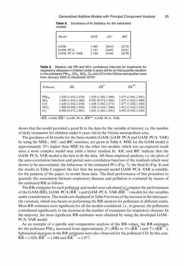
The goodness-of-fit results for the three models (GAM, GAM–PCA and GAM–PCA–VAR)by using the MSE-, AIC- and BIC-statistics, are given in Table 8. MSE for the GAM model isapproximately 35% higher than MSE for the other two models, which was an expected resultsince a more complex model may yield a better residual fit. AIC and BIC indicate that theGAM–PCA–VAR model is the best to fit the data. All these empirical analyses, i.e. the plots ofthe auto-correlation function and partial auto-correlation function of the residuals which wereshown to be uncorrelated, the behaviour of the estimated PCs (Fig. 7), the final fit (Fig. 8) andthe results in Table 8 support the fact that the proposed model GAM–PCA–VAR is suitable,for the purpose of the paper, to model these data. The final performance of this procedure toquantify the association between respiratory diseases and pollution is evaluated by means ofthe estimated RR as follows.
The RR-estimates for each pollutant and model were calculated to compare the performancesof the GAM (RR), GAM–PCA (RR
Å) and GAM–PCA–VAR (RR
ÅÅ) models for the variables
under consideration. The results are displayed in Table 9 in terms of the increase in the interquar-tile variation, which was based on performing the RR-analysis for pollutants at different scales.Most RR-estimates were significant for all the models considered, i.e., in general, the pollutantscontributed significantly to the increase in the number of treatments for respiratory diseases. Inthe majority, the most significant RR-estimates were obtained by using the developed GAM–PCA–VAR model.
As an example of a specific and comparative analysis of the RR-values, the RR-estimatesfor the pollutant PM10 increased from approximately 2% (RR) to 3% (RR
Å) and 7% (RR
ÅÅ).
Substantial increases in the RR-estimates were also observed for the pollutant CO. In this case,RR=1:020, RR
Å =1:048 and RRÅÅ =1:077.
26 J. B. de Souza, V. A. Reisen, G. C. Franco, M. Ispany, P. Bondon and J. Meri
Therefore, the developed GAM–PCA and GAM–PCA–VAR models generally showed morepronounced results than the conventional GAM for the expected increase in the number oftreatments for respiratory diseases, since the procedure allows a set of pollutants to be theexplanatory variable.
4. Conclusion
A hybrid of three statistical tools, the VAR model, PCA and the GAM, with Poisson marginaldistribution, was developed in this study to correlate the effect of atmospheric exposure to pol-lutants PM10, SO2, NO2, O3 and CO with the number of treatments for respiratory diseases inchildren under 6 years old in the Vitoria metropolitan area, Brazil, between 2005 and 2010. Be-cause of the complexity of the real data, a marginal Poisson assumption would not be the mostappropriate choice in this case since the series presented an overdispersion problem, which maycome from many features of the data such as changes in the mean and variance, and observa-tions with high levels (which increase substantially the variance) among others. Overdispersionis common in this kind of data, and the negative binomial and the generalized Poisson modelsare frequently used to account for this problem. For example, several statistics were proposedby Yang et al. (2007) in testing for a Poisson regression model against the negative binomialor generalized Poisson alternatives. However, the Poisson distribution is the most popular dis-tribution used in real applications when dealing with association between pollution and healthadverse problems. Besides, in this work the main objective was to investigate the effect of serialand cross-correlation of the pollutants that were included in the fit. Therefore, the use of a modelthat also handles overdispersion is an interesting and important issue to be considered in thecontext of the data analysed here. Hence this point, and the effect of high concentration levelsof the pollutants in the estimate of RR and bootstrap intervals for this quantity, will be part ofour future work.
The models developed were denoted here by GAM–PCA and GAM–PCA–VAR. The firstmodel used the PCs of the original pollutants as covariates in the GAM. The residuals of thismodel were fitted by using the SAR.1/.1/7 model, resulting in the final GAM–PCA model. Inthe second approach, a seasonal VAR(1) model was used to filter the original pollutants, beforebuilding the PCs. These modified PCs were then used as covariates in the GAM, resulting inthe hybrid model defined as GAM–PCA–VAR. In this model, the auto-correlation and cross-correlations of the PCs were removed by the VAR model.
A simulation study was conducted to evaluate the effect in the parameter estimates of GAMswhen the explanatory variables have serial correlation. The results showed that, if the auto-correlation in the independent variables is not taken into account, the GAM fit tends to under-estimate the true value of the coefficients and, consequently, it leads to biased RR-estimates.This means that a true effect of a pollutant in population health can be underestimated if themodel is not correctly adjusted. This issue was also recently explored in a different scenario byDionisio et al. (2016).
The adequacy of fit of the aforementioned models was compared by means of goodness-of-fitstatistics, such as MSE, AIC and BIC. On the basis of these quantities, in general, the threemethods displayed close results, where the standard GAM presented the worst performance.
The deleterious health effects of the exposure to pollutants for the population of children in theVitoria metropolitan area were obtained by estimating the relative risk RR of the GAM, GAM–PCA and GAM–PCA–VAR regression models. In general, the RR-estimates were significantfor all the models that were considered in the study. It should be stressed here that, in most cases,the estimated RR is larger for GAM–PCA–VAR when compared with the GAM. This can be

Generalized Additive Models with Principal Component Analysis 27
explained by the results obtained in the simulation study. Thus, the real effect of these pollutantsin a number of respiratory diseases can be underestimated if we use the standard GAM underan inappropriate scenario as was the case of the data used here. For example, for the pollutantPM10, the estimated relative risk increased from approximately 2% (RR) to 3% (RRÅ) and 7%(RRÅÅ). For the GAM–PCA model, an increase of 10:49μg m−3 (interquartile range) of theparticulate material (PM10) resulted in an RRÅ-value of 1.029 with 95% confidence interval(1.001,1.09), whereas for the GAM–PCA–VAR model a higher RRÅÅ-value of 1.075 with 95%confidence interval (1.001,1.092). Similar interpretations could be made for the other pollutantsand models developed.
In this study, the results that were obtained by using the GAM and GAM–PCA model werecoherent with those reported in Wang and Pham (2011), in which the morbidity was correlatedwith the atmospheric pollutant concentrations by using data registered in Korea. Although theserial correlation of the data was ignored by them when using PCA, the study also shows thatthe PCA technique improved the final relative risk estimates.
Acknowledgements
The authors thank the following agencies for their support: the National Council for Scien-tific and Technological Development (the Conselho Nacional de Desenvolvimento Cientıfico eTecnologico), the Brazilian Federal Agency for the Support and Evaluation of Graduate Ed-ucation (the Coordenacao de Aperfeicoamento de Pessoal de Nıvel Superior), Espırito SantoState Research Foundation (Fundacao de Amparo a Pesquisa do Espırito Santo) and the Mi-nas Gerais State Research Foundation (the Fundacao de Amparo a Pesquisa do Estado deMinas Gerais). Pascal Bondon thanks the Institute for Control and Decision of the UniversiteParis–Saclay. Part of this paper was written when Valderio A. Reisen was a visiting professor atCentraleSupelec. Valderio A. Reisen is indebted to CentraleSupelec for their financial support.
The authors are very grateful to the two referees and the Joint Editor for their suggestionsthat led to a markedly improved paper.
References
Akaike, H. (1973) Information theory and an extension of the maximum likelihood principle. In Proc. 2nd Int.Symp. Information Theory (eds B. N. Petrov and F. Csaki), pp. 267–281. Budapest: Akademiai Kiado.
Amemiya, T. (1985) Advanced Econometrics. Cambridge: Harvard University Press.Bakonyi, S. M. C., Danni-Oliveira, I. M., Martins, L. C. and Braga, A. L. F. (2004) Air pollution and respiratory
diseases among children in the city of Curitiba, Brazil. Rev. Saude Publ., 38, 675–700.Baxter, L. A., Finch, S. J., Lipfert, F. W. and Yu, Q. (1997) Comparing estimates of the effects of air pollution on
human mortality obtained using different regression methodologies. Risk Anal., 17, 273–278.Brockwell, P. J. and Davis, R. A. (1991) Time Series: Theory and Methods. New York: Springer.Campbell, M. J. (1994) Time series regression for counts: an investigation into the relationship between sudden
infant death syndrome and environmental temperature. J. R. Statist. Soc. A, 157, 191–208.Chen, R. J., Chu, C., Tan, J., Cao, J., Song, W., Xu, X., Jiang, C., Ma, W., Yang, C., Chen, B., Gui, Y. and Kan,
H. (2010) Ambient air pollution and hospital admission in Shanghai, China. J. Hazrd. Mater., 181, 234–240.Cotta, H., Reisen, V., Bondon, P. and Stummer, W. M. (2017) Robust estimation of covariance and correlation
functions of a stationary multivariate process. In Proc. Int. Conf. Time Series, Granada.Dalgaard, P. (2008) Introductory Statistics with R, 2nd edn. New York: Springer.Dionisio, K. L., Chang, H. H. and Baxter, L. K. (2016) A simulation study to quantify the impacts of exposure
measurement error on air pollution healh risk estimates in copollutant time-series models. Environ. Hlth, 15,article 114.
Dominici, F., McDermott, A., Zeger, S. L. and Samet, J. M. (2002) On the use of generalized additive models intime-series studies of air pollution and health. Am. J. Epidem., 156, 193–203.
Dominici, F., Peng, R. D., Bell, M. L., Pham, L., McDermott, A., Zeger, S. L. and Samet, J. M. (2006) Fineparticulate air pollution and hospital admission for cardiovascular and respiratory diseases. J. Am. Med. Ass.,295, 1127–1134.
28 J. B. de Souza, V. A. Reisen, G. C. Franco, M. Ispany, P. Bondon and J. Meri
Figueiras, A., Roca-Pardinas, J. and Cadarso-Suarez, C. (2005) A bootstrap method to avoid the effect of con-curvity in generalized additive models in time series of air pollution. J. Epidem. Commty Hlth, 59, 881–884.
Friedman, J. (1991) Multivariate adaptive regression splines. Ann. Statist., 19, 1–67.Greenaway-McGrevy, R., Han, Ch. and Sul, D. (2012) Estimating the number of common factors in serially
dependent approximate factor models. Econ. Lett., 116, 531–534.Hamilton, J. D. (1994) Time Series Analysis. Princeton: Princeton University Press.Hastie, T. J. and Tibshirani, R. J. (1990) Generalized Additive Models. London: Chapman and Hall.Hu, Y. and Tsay, R. S. (2014) Principal volatility component analysis. J. Bus. Econ. Statist., 32, 153–164.Johnson, R. A. and Wichern, D. W. (2007) Applied Multivariate Statistical Analysis, 6th edn. Englewood Cliffs:
Prentice Hall.Jolliffe, I. T. (2002) Principal Component Analysis, 2nd edn. New York: Springer.Kedem, B. and Fokianos, K. (2002) Regression Models for Time Series Analysis, 2nd edn. New York: Wiley.Lall, R., Ito, K. and Thurston, G. D. (2011) Distributed lag analysis of daily hospital admissions and source-
apportioned fine particle air pollution. Environ. Hlth Perspect., 119, 455–460.Matteson, D. S. and Tsay, R. S. (2011) Dynamic orthogonal components for multivariate time series. J. Am.
Statist. Ass., 106, 1450–1463.Michelozzi, P., Kirchmayer, U., Katsouyanni, K., Biggery, A., McGregor, G., Menne, B., Kassomenos, P., Ander-
son, H. R., Baccini, M., Accetta, G., Analytis, A. and Kosatsky, T. (2007) Assessment and prevention of acutehealth effects of weather conditions in Europe, the PHEWE project: background, objectives, design. Environ.Hlth, 6, no. 12, 1–10.
Ostro, B. D., Eskeland, G. S., Sanchez, J. M. and Feyzioglu, T. (1999) Air pollution and health effects: a study ofmedical visits among children in Santiago, Chile. Environ. Hlth Perspect., 107, 69–73.
Ramsey, T. O., Burnett, R. T. and Krewski, D. (2003) The effect of concurvity in generalized additive modelslinking mortality to ambient particulate matter. Epidemiology, 14, 18–23.
Reisen, V. A., Levy-Leduc, C., Cotta, H. H. A. and Toledo de Alburquerque, T. (2017) Long-memory modelunder outliers: an application to air pollution levels. In Environmental Science and Engineering: Air and NoisePollution, vol. 3 (eds B. R. Gurjar, P. Kumar and J. N. Govil), pp. 211–243. New Delhi: Studium.
Roberts, S. and Martin, M. (2006) Using supervised principal components analysis to assess multiple pollutanteffects. Environ. Hlth Perspect., 114, 1877–1882.
Schwartz, J. (2000) Harvesting and long term exposure effects in the relationship between air pollution andmortality. Am. J. Epidem., 151, 440–448.
Schwarz, G. E. (1978) Estimating the dimension of a model. Ann. Statist., 6, 461–464.Vanhatalo, E. and Kulachi, M. (2016) Impact of autocorrelation on principal components and their use in
statistical process control. Qual. Reliab. Engng Int., 32, 1483–1500.Wahba, G. (2001) Splines in nonparametric regression. In Encyclopedia of Environmetrics, vol. 4, 2nd edn (eds A.
H. El-Shaarawi and W. W. Piegorsch), pp. 2099–2112. New York: Wiley.Wang, Y. and Pham, H. (2011) Analyzing the effects of air pollution and mortality by generalized additive models
with robust principal components. Int. J. Syst. Assur. Engng Mangmnt, 2, 253–259.World Health Organization (2006) WHO Air Quality Guidelines for Particulate Matter, Ozone, Nitrogen Dioxide
and Sulphur Dioxide: Global Update 2005; Summary of Risk Assessment. Geneva: World Health OrganizationPress.
Yang, Z., Hardin, J. W., Addy, C. L. and Vuong, Q. H. (2007) Testing approaches for overdispersion in Poissonregression versus the generalized Poisson model. Biometr. J., 49, 565–584.
Zamprogno, B. (2013) PCA in time series with short and long-memory time series. PhD Thesis. Programa dePos-Graduacao em Engenharia Ambiental do Centro Tecnologico, Universidade Federal do Espirito Santo,Vitoria.
Zhao, J., Cao, J., Tian, S., Chen, Y., Zhang, Sh., Wang, Zh. and Zhou, X. (2014) A comparison between twoGAM models in quantifying relationships of environmental variables with fish richness and diversity indices.Aquat. Ecol., 48, 297–312.
Zou, G. (2004) A modified Poisson regression approach to prospective studies with binary data. Am. J. Epidem.,159, 702–706.