Embed Size (px)
Citation preview
University of Groningen
Generalized additive modeling to analyze dynamic phonetic dataWieling, Martijn
Published in:Journal of Phonetics
IMPORTANT NOTE: You are advised to consult the publisher's version (publisher's PDF) if you wish to cite fromit. Please check the document version below.
Document VersionFinal author's version (accepted by publisher, after peer review)
Publication date:2017
Link to publication in University of Groningen/UMCG research database
Citation for published version (APA):Wieling, M. (2017). Generalized additive modeling to analyze dynamic phonetic data: a tutorial focusing onarticulatory differences between L1 and L2 speakers of English. Journal of Phonetics.
CopyrightOther than for strictly personal use, it is not permitted to download or to forward/distribute the text or part of it without the consent of theauthor(s) and/or copyright holder(s), unless the work is under an open content license (like Creative Commons).
Take-down policyIf you believe that this document breaches copyright please contact us providing details, and we will remove access to the work immediatelyand investigate your claim.
Downloaded from the University of Groningen/UMCG research database (Pure): http://www.rug.nl/research/portal. For technical reasons thenumber of authors shown on this cover page is limited to 10 maximum.
Download date: 02-06-2018

Generalized additive modeling to analyze dynamic phonetic data: a tutorial focusing on articulatory differences between L1 and L2 speakers of English
Martijn Wieling University of Groningen, Haskins Laboratories
Abstract In phonetics many data sets are encountered which deal with dynamic data collected over time. Examples include dynamic formant trajectories, or tongue position trajectories obtained via electromagnetic articulography. Traditional approaches to analyzing this type of data generally aggregate data over a certain timespan, or only include measurements at a certain fixed time point (e.g., formant measurements at the midpoint of a vowel). While these types of analyses are relatively easy to understand and conduct, I argue in this paper for a more elaborate approach, generalized additive modeling, which is able to take into account the non-linear patterns over time while simultaneously taking into account subject and item-related variability. I will illustrate its use in this tutorial using articulatory trajectories from L1 and L2 speakers of English. All data and R code is made available for readers to replicate the analysis presented in this paper. 1. Introduction In phonetics, many types of data are collected, but more often than not these types of data involve some kind of measurements (which could have been) collected over multiple points in time. For example, in the most recent issue of Journal of Phonetics (Vol. 65, in progress with 6 papers available online at the time of writing), several papers focused on vowel formant measurements (Hay et al., 2017; Ots, 2017; Yang & Fox, 2017; Hualde et al., 2017) but all of these either analyzed formant measurements at pre-selected time points (Yang & Fox, 2017; Hualde et al., 2017), average formant measurements (Hay et al., 2017), or a simplified description of the formant contour (Ots, 2017). The single paper investigating articulatory measurements (Pastätter & Pouplier, 2017) also analyzed data for a single pre-selected time point (i.e. at the vowel midpoint). As the aforementioned studies illustrate, data is frequently simplified before conducting the analysis. While in some cases these simplified analyses may be appropriate given the research question, in other cases it may be more adequate to take into account all data. For example, when investigating language variation, dynamic formant trajectories have been found to reveal important (sociolinguistic) information which can be missed in the traditional single-point analysis (Van der Harst et al., 2014). An additional advantage of an analysis focusing on the whole time course of the signal is that it prevents having to make a subjective selection about what time window to average over. Of course, when analyzing data which have been collected over time, the linearity assumption is clearly not sufficient. Formant or tongue position trajectories generally show clear non-linear patterns, and assuming a linear relationship (e.g., as in linear mixed-effects regression modeling) is then not adequate anymore. To model non-linear patterns, there are various approaches one can use. For example, one can use growth curve analysis (e.g., Winter & Wieling, 2016) in which the researcher has to provide the specification of the non-linear pattern. Another popular approach is to use (a variant of) functional data analysis (e.g., Gubian et al. 2015, Cederbaum et al., 2016) where functional principal components analysis can be used to characterize different types of non-linear patterns. In this paper, however, we will focus on generalized additive models (GAMs; Hastie & Tibshirani, 1990; Wood, 2017). In generalized additive modeling the non-linear relationship between one or more predictors and the
dependent variable is determined automatically. While this type of analysis is not new, analyzing dynamic data in linguistics (often involving up to a few million data points) has been – until recently – computationally prohibitive. Nevertheless, various studies have recently been conducted which illustrate the potential of generalized additive modeling in linguistics and phonetics. For example, Wieling et al. (2011, 2014) used GAMs to model the non-linear influence of geography on dialectal pronunciation and lexical variation. In 2011, Wieling and colleagues used a generalized additive model to represent geography in a Dutch dialect dataset of over 225,000 observations, and used the fitted values of this model in a mixed-effects regression model (as random effects were not yet adequately implemented in the mgcv R package implementing generalized additive modeling). In 2014, however, the implementation was much improved, and Wieling and colleagues were able to model lexical variation in Tuscan dialects, using a logistic generalized additive model taking into account almost 400,000 observations, and modeling a four-way non-linear interaction (between geography, word frequency and word category) together with a rich random-effects structure. Time series data have been analyzed successfully with generalized additive modeling as well. Meulman et al. (2015) showed how to analyze EEG trajectories over time, while simultaneously assessing the continuous influence of age of acquisition in a dataset of over 1.6 million observations. Importantly, they highlighted the benefits of the GAM analysis over a more traditional ANOVA analysis. Nixon et al. (2016) illustrated how visual world (i.e. eye tracking) data could suitably be analyzed with GAMs in a study on Cantonese tone perception. In a useful tutorial, Sóskuthy (submitted) provided a hands-on introduction to GAMs, where he showed how to analyze formant trajectories over time using real-world data from Stuart-Smith et al. (2015). Winter and Wieling provided a tutorial in which they compared mixed-effects regression, growth curve analysis and generalized additive modeling in analyzing linguistic change over time. Finally, Wieling et al. (2016) used GAMs to analyze articulatory trajectories in order to assess differences in the tongue position over time of Dutch dialect speakers. In this study, we will illustrate the use of generalized additive modeling by analyzing a dataset of articulatory trajectories comparing native speakers of English to Dutch L2 speakers of English. In this paper, we will take a step-by-step approach in which we will start from a simple generalized additive model and extend this model step-by-step, allowing us to investigate all necessary concepts with respect to generalized additive modeling.
In our analysis, we will illustrate and explain the details of the model specification (in R), and also explain important concepts necessary to understand the analysis.1 Note, however, that this tutorial is not a complete introduction to GAMs. For that, we refer the interested reader to Wood (2017). 2. Research project description In this research project, our goal was to compare the pronunciation of native English speakers to non-native (Dutch) speakers of English. Speech learning models, such as Flege’s Speech Learning Model (SLM; Flege, 1995) or Best’s Perceptual Assimilation Model (Best, 1995), explain L2 pronunciation difficulties by considering the phonetic similarity of the speaker’s L1 and L2. Sound segments in the L2 that are very similar to those in the L1 (and map to the same category) are predicted to be harder to learn than those which are not (as these map to a new sound category). In this tutorial we focus on data collected for Dutch L2 speakers of English when they pronounce the sound /θ/ (which does not occur in their
1 This analysis is loosely based on several course lectures about generalized additive models. The slides of these lectures are available at: http://www.let.rug.nl/wieling/Statistics.
consonant inventory), and compare their pronunciations to those of native Southern Standard British English speakers. Based on earlier acoustic analyses of different data (Hanulika & Weber, 2012), Dutch speakers frequently substitute /θ/ with /t/, and here we will investigate if this also holds when taking an articulatory perspective. 3. Data collection procedure The Dutch L2 data was collected at the University of Groningen (20 speakers), whereas the English L1 data was collected at the University College London (22 speakers). (We also collected data for 29 German speakers at the University of Tübingen, but these data are not analyzed here to prevent complicating the tutorial.) Before conducting the experiment, ethical approval was obtained at the respective universities. Before the experiment, participants were informed about the nature and goal of the experiment and signed an informed consent form. Participants were reimbursed either via credit (Groningen) or monetarily (London) for their participation, which generally took about 90 minutes.
We collected data for 10 minimal pairs of English words for all speakers (i.e. ‘fate’-‘faith’, ‘fort’-‘forth’, ‘kit’-‘kith’, ‘mitt’-‘myth’, ‘tent’-‘tenth’, ‘tank’-‘thank’, ‘team’-‘theme’, ‘tick’-‘thick’, ‘ties’-‘thighs’, and ‘tongs’-‘thongs’). Each pronunciation was preceded and succeeded by the pronunciation of /ə/ in order to ensure a neutral articulatory position. Each word was pronounced twice, and the order was randomized. While the speakers were pronouncing these words, we tracked the movement of their tongue and lips using a portable 16-channel Wave electromagnetic articulography (EMA) device (Northern Digital Inc.) at a sampling rate of 100 Hz. Sensors were glued to the tongue and lips with PeriAcryl 90HV dental glue. The acoustic data (collected using an Audio-Technica AT875R microphone) was automatically synchronized with the articulatory data.
In this tutorial, we only focus on the anterior-posterior position of the T1 sensor (positioned about 0.5-1 cm behind the tongue tip), as articulatory differences between /t/ and /θ/ should be most clearly apparent there. After collecting, the articulatory data was head-corrected using four sensors attached to the head (left and right mastoid process, the forehead, and the upper incisor) whose movement was filtered at 5 Hz. Using a biteplate recording (with three sensors attached to a plastic rectangular card; see Wieling et al., 2016), the data for each speaker were rotated relative to the occlusal plane. The data were subsequently segmented on the basis of the articulatory gestures (i.e. from the gestural onset of the initial sound to the gestural offset of the final sound; using MView; Tiede, 2005) and time-normalized between 0 (start of the word) to 1 (end of the word). Furthermore, the T1 sensor positions were normalized for each speaker by z-transforming the positions per speaker (i.e. subtracting the mean and dividing by the standard deviation; the mean and standard deviation per speaker were obtained on the basis of all 200-250 utterances elicited in the context of the broader experiment in which the present data was collected). Higher values signify more anterior positions, whereas lower values indicate more posterior positions. In this study, we will analyze filtered data (at 20 Hz), as this was the data on which the articulatory segmentation was based. However, filtering is not necessary as the generalized additive modeling analysis will essentially smooth the data. In fact, it is even beneficial to analyze raw instead of filtered data, as this will result in less autocorrelation in the residuals (see Section 4.8 for an explanation). 4. Generalized additive modeling: step-by-step analysis A generalized additive model can be seen as a regression model which is able to model non-linear patterns. Rather than explaining the basic concepts underlying generalized additive modeling at the start (e.g., how are non-linear patterns modeled, etc.), in this tutorial, we will explain the concepts when we first encounter them in the analysis. Importantly, this
tutorial will not focus on the underlying mathematics, but rather take a more hands-on approach. For more (mathematical) background, we refer the reader to the excellent, recently revised book of Simon Wood on generalized additive modeling (Wood, 2017).
To create a generalized additive model we will use the mgcv package in R (version 1.8-18; Wood, 2011; Wood, 2017). Furthermore, for convenient plotting functions, we will use the itsadug R package (version 2.2.0; van Rij et al, 2016). Both can be loaded via the library command (e.g., library(mgcv)). (Note that R commands as well as the output will be explicitly marked by using a monospace font.)
Instead of starting immediately with the appropriate model for our data, we will start with a simple model and make the model gradually more complex, eventually leading to the model appropriate for our data. Particularly, we will first discuss models which do not include any random effects, even though this is clearly inappropriate (given that speakers pronounce multiple words). Consequently, please take into account that the p-values and confidence bands will be overconfident for these first few models.
Of course, over time the function calls or function parameters may become outdated, while this tutorial text, once published, will remain fixed. Therefore, we will endeavor to keep the associated paper package (available at the Mind Research Repository, http://openscience.uni-leipzig.de, and the first author’s personal website, http://www.martijnwieling.nl) which includes all data, code, and output, up-to-date. 4.1 The dataset Our dataset, dat, has the following structure (only the first six out of 126,117 lines are shown): Speaker Lang Word Sound Loc Trial Time Pos
1 VENI_EN_1 EN tick T Front 1 0.00000000 -0.4100307
2 VENI_EN_1 EN tick T Front 1 0.01612903 -0.4209585
3 VENI_EN_1 EN tick T Front 1 0.03225806 -0.4449649
4 VENI_EN_1 EN tick T Front 1 0.04838710 -0.4876798
5 VENI_EN_1 EN tick T Front 1 0.06451613 -0.5592895
6 VENI_EN_1 EN tick T Front 1 0.08064516 -0.6543947
The first column (i.e. variable), Speaker, shows the speaker ID, whereas the second
column, Lang, shows the native language of the speaker (EN for native English speakers, or NL for native Dutch speakers). The third column, Word, shows the item label. Column four,
Sound, contains either T or TH for minimal pairs involving the /t/ or the /θ/, respectively. Column five, Loc, contains either the value Start or the value End, indicating where in the word the sound /t/ or /θ/ occurs (e.g., for the words ‘faith’ and ‘fate’ this is at the end of the word). The sixth column, Trial, contains the trial number at which the word was pronounced by the speaker. The final two columns, Time and Pos, contain the normalized time point and the associated (standardized) anterior position of the T1 sensor. 4.2 A first (linear) model For simplicity, we will illustrate the generalized additive modeling approach by focusing only on the minimal pair ‘fate’-‘faith’. We will use this example to illustrate all necessary concepts, but we will later extend our analysis to all words.
The first model we construct is:
m1 <- bam(Pos ~ Word, data=dat, method="fREML")
This model simply estimates the average (constant) anterior position difference between the two words (‘fate’ and ‘faith’), and is shown to illustrate the general model specification. We use the function bam to fit a generalized additive model. (The alternative function gam is more precise, but becomes prohibitively slow for complex models which are fit to datasets exceeding 10,000 data points.) The first parameter of the function is the formula reflecting the model specification, in this case: Pos ~ Word. The first variable of the formula, Pos, is the dependent variable (the anterior position of the T1 sensor). The dependent variable is followed by the tilde (~), after which one or more independent variables are added. In this case, the inclusion of a single predictor, Word, allows the model to only estimate a constant difference between its two levels (‘faith’ versus ‘fate’; the latter word has been set as the reference level of the predictor). The parameter data is set to the name of the data frame in which the values of the dependent and independent variables are stored (in this case: dat). The third parameter (method) specifies the smoothing parameter estimation method, which is currently set to the default of "fREML", fast restricted maximum likelihood estimation. This is the one of the fastest fitting methods, but it is important to keep in mind that models fit with (f)REML cannot be compared when the models differ in their fixed effects (i.e. the predictors in which we are generally interested; see Section 4.7 for more details). In that case, method should be set to "ML" (maximum likelihood estimation), which is much slower. To obtain a summary of the model we can use the following command in R:
(smry1 <- summary(m1)) Note that it is generally good practice to store the summary in a variable, since the summary of a complex model might take a while to compute. The summary (which is printed as the full command is put between parentheses) shows the following: Family: gaussian
Link function: identity
Formula:
Pos ~ Word
Parametric coefficients:
Estimate Std. Error t value Pr(>|t|)
(Intercept) 0.12164 0.01047 11.62 <2e-16 ***
Wordfaith 0.35773 0.01461 24.49 <2e-16 ***
---
Signif. codes: 0 ‘***’ 0.001 ‘**’ 0.01 ‘*’ 0.05 ‘.’ 0.1 ‘ ’ 1
R-sq.(adj) = 0.0453 Deviance explained = 4.54%
-REML = 15417 Scale est. = 0.673 n = 12622
The top lines show that we use a Gaussian model with an identity link function (i.e. we use the original, non-transformed, dependent variable), together with the model formula. The next block shows the parametric coefficients. As usual in regression, the intercept is the value of the dependent variable when all numerical predictors are equal to 0 and nominal variables are at their reference level. Since the reference level for the nominal variable Word is ‘fate’, this means the average anterior position for the word ‘fate’ for all speakers is
0.12. The line associated with Wordfaith (the non-reference level, i.e. faith, is appended to the variable name) indicates that the anterior position for the word ‘faith’ is about 0.36 higher than for the word ‘fate’, and that this difference is significant with a very small p-value (at least, according to this analysis, which does not yet take into account the random-effects structure into account). The final lines show some goodness-of-fit statistics with both the adjusted r2, the explained deviance, the –REML score (as the score is negative), the estimate of the scale parameter of the model, and the number of data points fitted. 4.3 Modeling non-linear patterns Of course, we are not only interested in a constant difference between the two words, but also in the anterior position of the T1 sensor over time. A generalized additive model allows us to assess if there are non-linear patterns in our data by using so-called smooths. These smooths model non-linear patterns by combining a pre-specified number of basis functions. For example, a cubic regression smooth constructs a non-linear pattern by joining several cubic polynomials. The default type of smooth, which we will use in this tutorial, is the thin plate regression spline. The thin plate regression spline is a computationally efficient approximation of the optimal thin plate spline (Wood, 2003). The thin plate regression spline models a non-linear pattern by combining increasingly complex non-linear basis functions (see Figure 1). Each basis function is first multiplied by a coefficient (i.e. the magnitude of the contribution of that basis function) and then all resulting patterns are summed to yield the final (potentially) non-linear pattern. While modeling non-linear patterns may seem as an approach which is bound to lead to overfitting, GAMs apply a penalization to non-linearity (i.e. ‘wigglyness’) to prevent this. Rather than minimizing the error only (i.e. the difference between the fitted values and the actual values), GAMs minimize a combination between the error and a non-linearity penalty. The optimal tradeoff between these two factors is determined on the basis of cross-validation. Consequently, a generalized additive model will only identify a non-linear effect if there is substantial support for such a pattern in the data, but it will also detect a linear effect if there is only support for that. With respect to the thin plate regression spline basis functions visualized in Figure 1, especially the more complex non-linear patterns will be more heavily penalized (i.e. have coefficients closer to zero).
To fit a generalized additive model extending m1 by including a non-linear pattern over time for both groups separately, the following model can be specified (we excluded the method parameter as it is set to the default value of "fREML"):
m2 <- bam(Pos ~ Word + s(Time, by=Word, bs="tp", k=10), data=dat)
The text in boldface shows the additional term compared to model m1. The function s sets up a smooth over the first parameter (Time), separately for each level of the nominal variable indicated by the by-parameter (i.e. Word). The bs-parameter specifies the type of smooth, and in this case is set to "tp", the default thin plate regression spline. The k-parameter, finally, specifies the maximum number of basis functions which can be used for the construction of the spline. In this case, the maximum is set to 10 basis functions (which is equal to the, arbitrary, default). Since the smooth type and the number of basis functions are both set to their default, a simpler specification of the smooth is s(Time, by=Word). If the by-parameter would be left out, the model would fit only a single non-linear pattern, and not a separate pattern per word. The summary of model m2 shows the following (starting from the parametric coefficients):
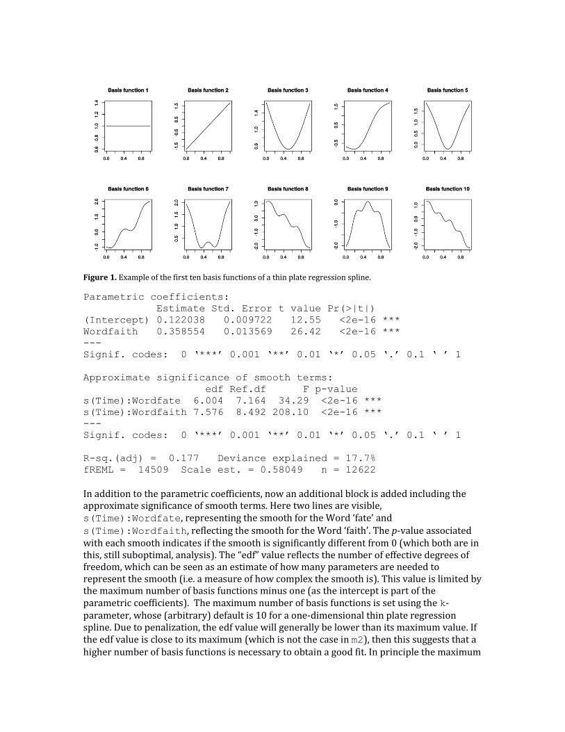
Figure 1. Example of the first ten basis functions of a thin plate regression spline.
Parametric coefficients:
Estimate Std. Error t value Pr(>|t|)
(Intercept) 0.122038 0.009722 12.55 <2e-16 ***
Wordfaith 0.358554 0.013569 26.42 <2e-16 ***
---
Signif. codes: 0 ‘***’ 0.001 ‘**’ 0.01 ‘*’ 0.05 ‘.’ 0.1 ‘ ’ 1
Approximate significance of smooth terms:
edf Ref.df F p-value
s(Time):Wordfate 6.004 7.164 34.29 <2e-16 ***
s(Time):Wordfaith 7.576 8.492 208.10 <2e-16 ***
---
Signif. codes: 0 ‘***’ 0.001 ‘**’ 0.01 ‘*’ 0.05 ‘.’ 0.1 ‘ ’ 1
R-sq.(adj) = 0.177 Deviance explained = 17.7%
fREML = 14509 Scale est. = 0.58049 n = 12622
In addition to the parametric coefficients, now an additional block is added including the approximate significance of smooth terms. Here two lines are visible, s(Time):Wordfate, representing the smooth for the Word ‘fate’ and
s(Time):Wordfaith, reflecting the smooth for the Word ‘faith’. The p-value associated with each smooth indicates if the smooth is significantly different from 0 (which both are in this, still suboptimal, analysis). The “edf” value reflects the number of effective degrees of freedom, which can be seen as an estimate of how many parameters are needed to represent the smooth (i.e. a measure of how complex the smooth is). This value is limited by the maximum number of basis functions minus one (as the intercept is part of the parametric coefficients). The maximum number of basis functions is set using the k-parameter, whose (arbitrary) default is 10 for a one-dimensional thin plate regression spline. Due to penalization, the edf value will generally be lower than its maximum value. If the edf value is close to its maximum (which is not the case in m2), then this suggests that a higher number of basis functions is necessary to obtain a good fit. In principle the maximum
value of the k-parameter can be set as high as the number of unique values in the data, as penalization will result in the appropriate shape. However, allowing for more complexity negatively impacts computation time. The number of basis functions is also indicative of the amount of non-linearity of the smooth. If the edf value for a certain smooth is (close to) 1, this means that the pattern is linear (i.e. cf. the second basis function in Figure 1). A value greater than 1 indicates that more basis functions (besides the linear pattern) are necessary, and therefore the pattern is non-linear. The Ref.df value is the reference number of degrees of freedom used for hypothesis testing (on the basis of the associated F-value). 4.4 Visualizing GAMs While it is possible to summarize a linear pattern in only a single line, this is obviously not possible for a non-linear pattern. Correspondingly, visualization is essential to interpret the non-linear patterns. The command: plot(m2) yields the visualizations shown in Figure 2. It is important to realize that this plotting function only visualizes the two non-linear patterns without taking into account anything else in the model. This means that only the partial effects are visualized. It is also good to keep in mind that the smooths themselves are centered (i.e. move around y = 0). So visualizing the smooths in this way, i.e. as a partial effect, is insightful to identify the non-linear patterns, but it does not give any information about the relative height of the smooths. For this we need to take into account the full model (i.e. the fitted values). Particularly, the intercept and the constant difference between the two smooths shown in the parametric part of the model needs to be taken into account. For this type of visualization we use the function plot_smooth from the itsadug package as follows:
plot_smooth(m2, view="Time", plot_all="Word", rug=FALSE)
The first parameter is the name of the stored model. The parameter view is set to the name of the variable visualized on the x-axis. The parameter plot_all should be set (to the name of the nominal variable) if smooths need to be displayed for all levels of a nominal variable. This is generally the name of the variable set using the by-parameter in the smooth specification. If the parameter is excluded, it only shows a graph for a single level (a notification will report which level is shown in case there are multiple levels). The final parameter rug is used to show or suppress small vertical lines on the x-axis for all individual data points. Since there are so many unique values, we suppress these vertical lines here by setting the value of the parameter to FALSE. Figure 3 shows the results of this call by visualizing both patterns in a single graph. It is clear that the smooths are not centered (i.e. they represent full effects, rather than partial effects), and that the ‘faith’-curve is above the ‘fate’-curve, reflecting that the /θ/ is pronounced further in the front of the mouth. The shapes of the curves are, as would be expected, identical to the partial effects shown in Figure 2.
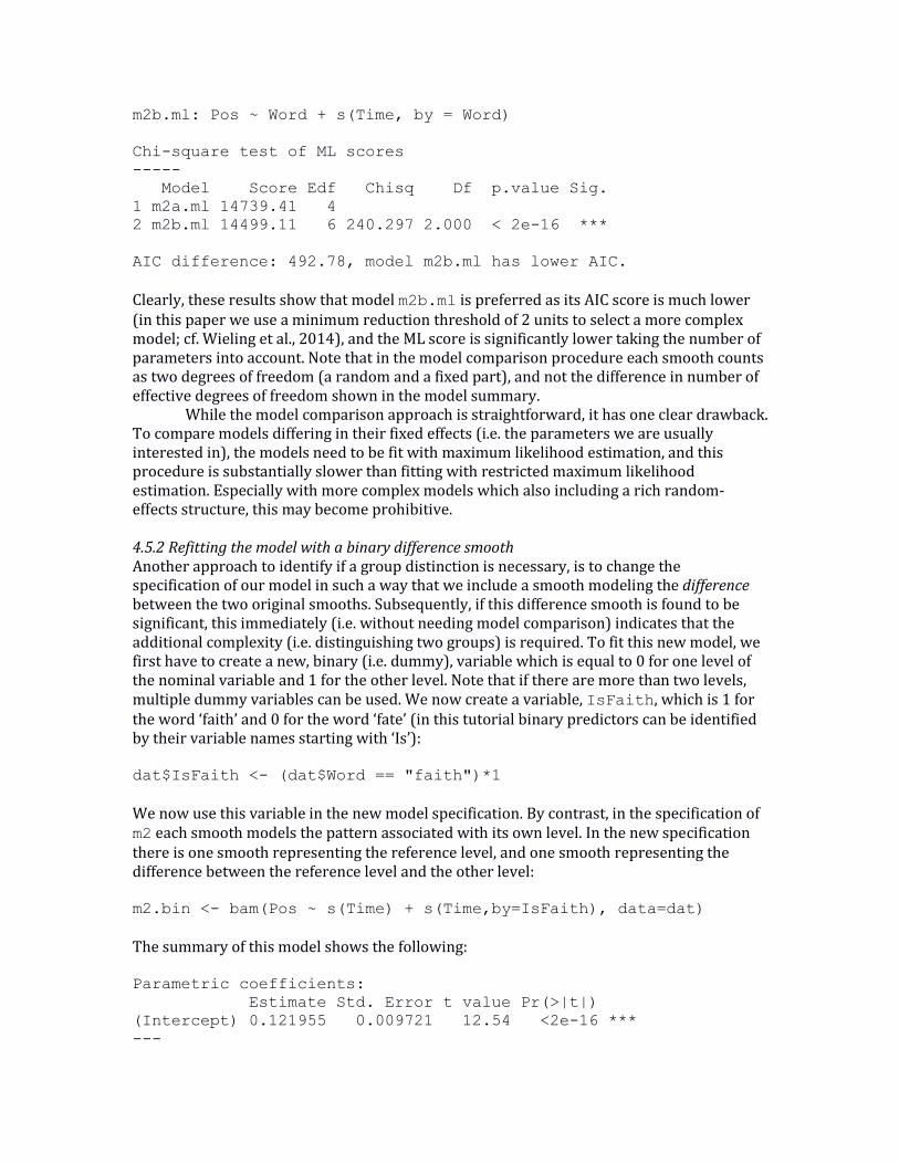
To visualize the difference, we can use the itsadug function plot_diff as follows:
plot_diff(m2, view="Time", comp=list(Word=c("faith","fate")))
The parameters are similar to those of the plot_smooth function, with the addition of the
comp parameter which requires a list of one or more variables together with two levels which should be compared. In this case, the first word (i.e. ‘faith’) is contrasted with the second word (i.e. ‘fate’) in the plot. Figure 4 shows this difference.
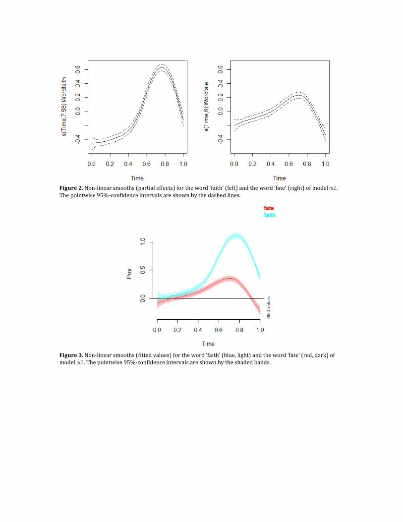
Figure 2. Non-linear smooths (partial effects) for the word ‘faith’ (left) and the word ‘fate’ (right) of model m2. The pointwise 95%-confidence intervals are shown by the dashed lines.
Figure 3. Non-linear smooths (fitted values) for the word ‘faith’ (blue, light) and the word ‘fate’ (red, dark) of model m2. The pointwise 95%-confidence intervals are shown by the shaded bands.
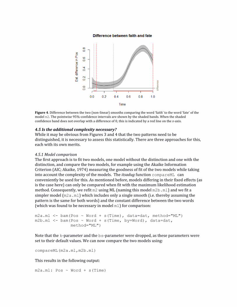
Figure 4. Difference between the two (non-linear) smooths comparing the word ‘faith’ to the word ‘fate’ of the model m2. The pointwise 95%-confidence intervals are shown by the shaded bands. When the shaded confidence band does not overlap with a difference of 0, this is indicated by a red line on the x-axis.
4.5 Is the additional complexity necessary? While it may be obvious from Figures 3 and 4 that the two patterns need to be distinguished, it is necessary to assess this statistically. There are three approaches for this, each with its own merits. 4.5.1 Model comparison The first approach is to fit two models, one model without the distinction and one with the distinction, and compare the two models, for example using the Akaike Information Criterion (AIC; Akaike, 1974) measuring the goodness of fit of the two models while taking into account the complexity of the models. The itsadug function compareML can conveniently be used for this. As mentioned before, models differing in their fixed effects (as is the case here) can only be compared when fit with the maximum likelihood estimation method. Consequently, we refit m2 using ML (naming this model m2b.ml) and we fit a simpler model (m2a.ml) which includes only a single smooth (i.e. thereby assuming the pattern is the same for both words) and the constant difference between the two words (which was found to be necessary in model m1) for comparison: m2a.ml <- bam(Pos ~ Word + s(Time), data=dat, method="ML")
m2b.ml <- bam(Pos ~ Word + s(Time, by=Word), data=dat,
method="ML")
Note that the k-parameter and the bs-parameter were dropped, as these parameters were set to their default values. We can now compare the two models using: compareML(m2a.ml,m2b.ml)
This results in the following output: m2a.ml: Pos ~ Word + s(Time)
m2b.ml: Pos ~ Word + s(Time, by = Word)
Chi-square test of ML scores
-----
Model Score Edf Chisq Df p.value Sig.
1 m2a.ml 14739.41 4
2 m2b.ml 14499.11 6 240.297 2.000 < 2e-16 ***
AIC difference: 492.78, model m2b.ml has lower AIC.
Clearly, these results show that model m2b.ml is preferred as its AIC score is much lower (in this paper we use a minimum reduction threshold of 2 units to select a more complex model; cf. Wieling et al., 2014), and the ML score is significantly lower taking the number of parameters into account. Note that in the model comparison procedure each smooth counts as two degrees of freedom (a random and a fixed part), and not the difference in number of effective degrees of freedom shown in the model summary. While the model comparison approach is straightforward, it has one clear drawback. To compare models differing in their fixed effects (i.e. the parameters we are usually interested in), the models need to be fit with maximum likelihood estimation, and this procedure is substantially slower than fitting with restricted maximum likelihood estimation. Especially with more complex models which also including a rich random-effects structure, this may become prohibitive. 4.5.2 Refitting the model with a binary difference smooth Another approach to identify if a group distinction is necessary, is to change the specification of our model in such a way that we include a smooth modeling the difference between the two original smooths. Subsequently, if this difference smooth is found to be significant, this immediately (i.e. without needing model comparison) indicates that the additional complexity (i.e. distinguishing two groups) is required. To fit this new model, we first have to create a new, binary (i.e. dummy), variable which is equal to 0 for one level of the nominal variable and 1 for the other level. Note that if there are more than two levels, multiple dummy variables can be used. We now create a variable, IsFaith, which is 1 for the word ‘faith’ and 0 for the word ‘fate’ (in this tutorial binary predictors can be identified by their variable names starting with ‘Is’): dat$IsFaith <- (dat$Word == "faith")*1
We now use this variable in the new model specification. By contrast, in the specification of m2 each smooth models the pattern associated with its own level. In the new specification there is one smooth representing the reference level, and one smooth representing the difference between the reference level and the other level: m2.bin <- bam(Pos ~ s(Time) + s(Time,by=IsFaith), data=dat)
The summary of this model shows the following: Parametric coefficients:
Estimate Std. Error t value Pr(>|t|)
(Intercept) 0.121955 0.009721 12.54 <2e-16 ***
---
Signif. codes: 0 ‘***’ 0.001 ‘**’ 0.01 ‘*’ 0.05 ‘.’ 0.1 ‘ ’ 1
Approximate significance of smooth terms:
edf Ref.df F p-value
s(Time) 6.394 7.450 34.26 <2e-16 ***
s(Time):IsFaith 7.209 8.277 146.29 <2e-16 ***
---
Signif. codes: 0 ‘***’ 0.001 ‘**’ 0.01 ‘*’ 0.05 ‘.’ 0.1 ‘ ’ 1
R-sq.(adj) = 0.177 Deviance explained = 17.7%
fREML = 14506 Scale est. = 0.58047 n = 12622
The model specification is now quite different. The first part, s(Time), indicates the pattern over time which is included irrespective of the value of IsFaith (i.e. irrespective
of the word). The second part s(Time,by=IsFaith) has a special interpretation, due to IsFaith being a binary variable. If (and only if) the by-parameter is set to a binary variable, the smooth is equal to 0 whenever the binary variable equals 0. If the binary by-variable equals 1, it models a non-linear pattern which (importantly) does not have to be centered. In contrast to a normal smooth (or multiple smooths distinguished by the by-parameter set to a nominal variable) which is centered (e.g., see Figure 2), these so-called binary smooths also model the constant difference between the two levels (i.e. comparing when IsFaith equals 1 for the word ‘faith’, and when IsFaith equals 0 for the word
‘fate’). This is also the reason that the predictor IsFaith (or Word) should not be included as a fixed-effect factor.
The interpretation of this model is now as follows. When IsFaith = 0 (i.e. for the word ‘fate’), the position of the sensor is modeled by s(Time) + 0. This means that the first s(Time) represents the smooth for the word ‘fate’ (the reference level). When IsFaith = 1 (i.e. for the word ‘faith’), the position of the sensor is modeled by s(Time) +
s(Time,by=IsFaith). Given that s(Time) models the pattern for the word ‘fate’, and both smooths together model the pattern for the word ‘faith’, it logically follows that s(Time,by=IsFaith)models the difference between the non-linear patterns of ‘faith’ and ‘fate’. That this is indeed the case, can be seen by visualizing the binary difference smooth (i.e. the partial effect) directly via plot(m2.bin, select=2, shade=TRUE). Note that the parameter select determines which smooth to visualize (the second
smooth in the model summary, s(Time):IsFaith), whereas the parameter shade is used to determine if the confidence interval needs to be shaded (i.e. when set to TRUE), or if dashed lines should be used (i.e. when set to FALSE, the default). The horizontal line was added with the command abline(h=0). The graphical results of these commands are shown in Figure 5, and this graph matches Figure 4. It is also clear that the partial effect includes the intercept difference, given that the smooth is not centered. Importantly, the model summary shows that the non-linear pattern for the difference between the two words is highly significant (at least in this model specification which excludes the required random-effects structure), thereby alleviating the need for model comparison.
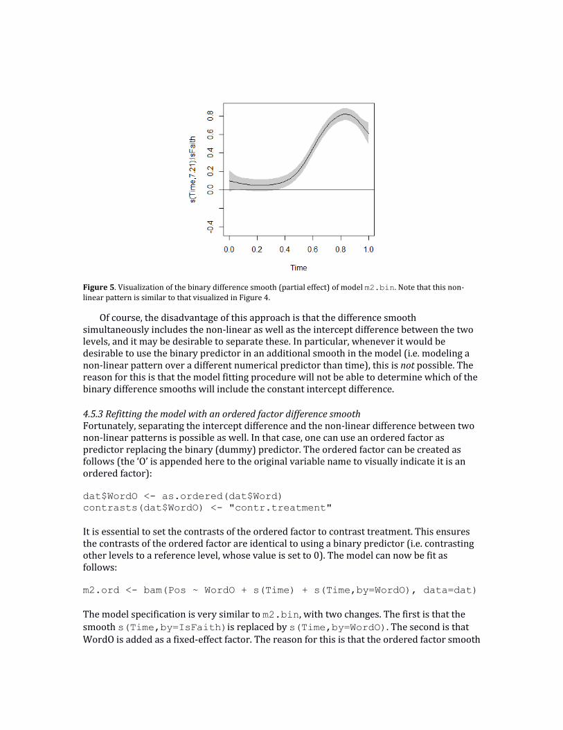
Figure 5. Visualization of the binary difference smooth (partial effect) of model m2.bin. Note that this non-linear pattern is similar to that visualized in Figure 4.
Of course, the disadvantage of this approach is that the difference smooth simultaneously includes the non-linear as well as the intercept difference between the two levels, and it may be desirable to separate these. In particular, whenever it would be desirable to use the binary predictor in an additional smooth in the model (i.e. modeling a non-linear pattern over a different numerical predictor than time), this is not possible. The reason for this is that the model fitting procedure will not be able to determine which of the binary difference smooths will include the constant intercept difference.
4.5.3 Refitting the model with an ordered factor difference smooth Fortunately, separating the intercept difference and the non-linear difference between two non-linear patterns is possible as well. In that case, one can use an ordered factor as predictor replacing the binary (dummy) predictor. The ordered factor can be created as follows (the ‘O’ is appended here to the original variable name to visually indicate it is an ordered factor):
dat$WordO <- as.ordered(dat$Word)
contrasts(dat$WordO) <- "contr.treatment"
It is essential to set the contrasts of the ordered factor to contrast treatment. This ensures the contrasts of the ordered factor are identical to using a binary predictor (i.e. contrasting other levels to a reference level, whose value is set to 0). The model can now be fit as follows:
m2.ord <- bam(Pos ~ WordO + s(Time) + s(Time,by=WordO), data=dat)
The model specification is very similar to m2.bin, with two changes. The first is that the
smooth s(Time,by=IsFaith)is replaced by s(Time,by=WordO). The second is that WordO is added as a fixed-effect factor. The reason for this is that the ordered factor smooth
is centered (as the normal smooths), and the constant difference between the two words needs to be included explicitly. Fitting the model yields the following model summary: Parametric coefficients:
Estimate Std. Error t value Pr(>|t|)
(Intercept) 0.122006 0.009721 12.55 <2e-16 ***
WordOfaith 0.358589 0.013569 26.43 <2e-16 ***
---
Signif. codes: 0 ‘***’ 0.001 ‘**’ 0.01 ‘*’ 0.05 ‘.’ 0.1 ‘ ’ 1
Approximate significance of smooth terms:
edf Ref.df F p-value
s(Time) 6.394 7.450 34.26 <2e-16 ***
s(Time):WordOfaith 6.209 7.277 71.06 <2e-16 ***
---
Signif. codes: 0 ‘***’ 0.001 ‘**’ 0.01 ‘*’ 0.05 ‘.’ 0.1 ‘ ’ 1
R-sq.(adj) = 0.177 Deviance explained = 17.7%
fREML = 14506 Scale est. = 0.58047 n = 12622
This model is essentially identical to model m2.bin (i.e. the AIC and the predictions of the
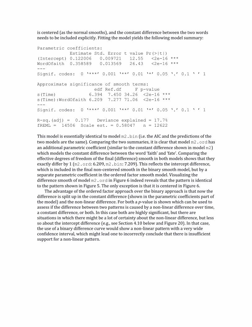
two models are the same). Comparing the two summaries, it is clear that model m2.ord has an additional parametric coefficient (similar to the constant difference shown in model m2) which models the constant difference between the word ‘faith’ and ‘fate’. Comparing the effective degrees of freedom of the final (difference) smooth in both models shows that they exactly differ by 1 (m2.ord: 6.209, m2.bin: 7.209). This reflects the intercept difference, which is included in the final non-centered smooth in the binary smooth model, but by a separate parametric coefficient in the ordered factor smooth model. Visualizing the difference smooth of model m2.ord in Figure 6 indeed reveals that the pattern is identical to the pattern shown in Figure 5. The only exception is that it is centered in Figure 6.
The advantage of the ordered factor approach over the binary approach is that now the difference is split up in the constant difference (shown in the parametric coefficients part of the model) and the non-linear difference. For both a p-value is shown which can be used to assess if the difference between two patterns is caused by a non-linear difference over time, a constant difference, or both. In this case both are highly significant, but there are situations in which there might be a lot of certainty about the non-linear difference, but less so about the intercept difference (e.g., see Section 4.10 below and Figure 20). In that case, the use of a binary difference curve would show a non-linear pattern with a very wide confidence interval, which might lead one to incorrectly conclude that there is insufficient support for a non-linear pattern.
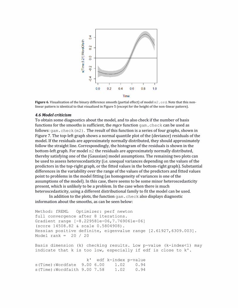
Figure 6. Visualization of the binary difference smooth (partial effect) of model m2.ord. Note that this non-linear pattern is identical to that visualized in Figure 5 (except for the height of the non-linear pattern).
4.6 Model criticism To obtain some diagnostics about the model, and to also check if the number of basis functions for the smooths is sufficient, the mgcv function gam.check can be used as
follows: gam.check(m2). The result of this function is a series of four graphs, shown in Figure 7. The top-left graph shows a normal quantile plot of the (deviance) residuals of the model. If the residuals are approximately normally distributed, they should approximately follow the straight line. Correspondingly, the histogram of the residuals is shown in the bottom-left graph. For model m2 the residuals are approximately normally distributed, thereby satisfying one of the (Gaussian) model assumptions. The remaining two plots can be used to assess heteroscedasticity (i.e. unequal variances depending on the values of the predictors in the top-right graph, or the fitted values in the bottom-right graph). Substantial differences in the variability over the range of the values of the predictors and fitted values point to problems in the model fitting (as homogeneity of variances is one of the assumptions of the model). In this case, there seems to be some minor heteroscedasticity present, which is unlikely to be a problem. In the case when there is much heteroscedasticity, using a different distributional family to fit the model can be used.
In addition to the plots, the function gam.check also displays diagnostic information about the smooths, as can be seen below: Method: fREML Optimizer: perf newton
full convergence after 8 iterations.
Gradient range [-8.229581e-06,7.769061e-06]
(score 14508.82 & scale 0.5804908).
Hessian positive definite, eigenvalue range [2.61927,6309.003].
Model rank = 20 / 20
Basis dimension (k) checking results. Low p-value (k-index<1) may
indicate that k is too low, especially if edf is close to k'.
k' edf k-index p-value
s(Time):Wordfate 9.00 6.00 1.02 0.94
s(Time):Wordfaith 9.00 7.58 1.02 0.94
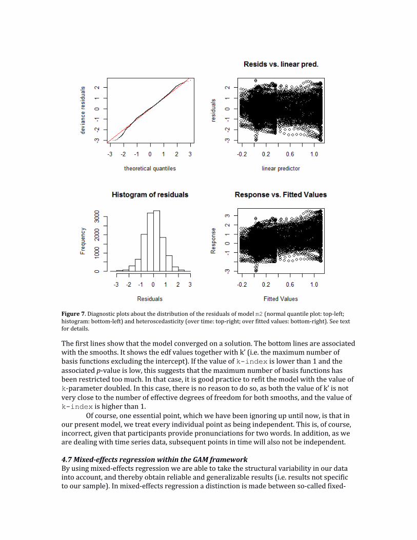
Figure 7. Diagnostic plots about the distribution of the residuals of model m2 (normal quantile plot: top-left; histogram: bottom-left) and heteroscedasticity (over time: top-right; over fitted values: bottom-right). See text for details.
The first lines show that the model converged on a solution. The bottom lines are associated with the smooths. It shows the edf values together with k’ (i.e. the maximum number of basis functions excluding the intercept). If the value of k-index is lower than 1 and the associated p-value is low, this suggests that the maximum number of basis functions has been restricted too much. In that case, it is good practice to refit the model with the value of k-parameter doubled. In this case, there is no reason to do so, as both the value of k’ is not very close to the number of effective degrees of freedom for both smooths, and the value of k-index is higher than 1.
Of course, one essential point, which we have been ignoring up until now, is that in our present model, we treat every individual point as being independent. This is, of course, incorrect, given that participants provide pronunciations for two words. In addition, as we are dealing with time series data, subsequent points in time will also not be independent. 4.7 Mixed-effects regression within the GAM framework By using mixed-effects regression we are able to take the structural variability in our data into account, and thereby obtain reliable and generalizable results (i.e. results not specific to our sample). In mixed-effects regression a distinction is made between so-called fixed-
effect factors and random-effect factors. Fixed-effect factors are nominal (i.e. factor) variables with a small number of levels, out of which all (or most) levels are included in the data. For example, both native and non-native speakers are present in our data. In addition, numerical predictors are always part of the fixed-effects specification of the model. In a regular linear (non-mixed-effects) regression model, the fixed effects are all predictors which are included in the model. Random-effect factors are those factors which introduce systematic variation, generally have a large number of levels and which the researcher would like to generalize over. In many studies in linguistics, the random-effect factors include participant and word, as the levels of these studies are sampled from a much larger population (i.e. other participants and other words could have been included). Note that for the present small dataset word is a fixed-effect factor, given that we are currently only interested in the difference between these specific words.
With respect to random-effect factors, it is important to distinguish random intercepts and random slopes. Some speakers (or words) will on average have a more anterior position than others, and this structural variability is captured by a by-speaker (or by-word) random intercept. Random slopes simply allow the influence of a predictor to vary for each level of the random-effect factor. For example, the difference between the /t/ and the /θ/-words may vary per speaker. It is essential to assess which random intercepts and slopes need to be included, as failing to include a necessary random slope may yield p-values which are overconfident. For example, suppose that ninety percent of the speakers shows a negligible difference between the /t/ and the /θ/, and the remaining ten percent of the speakers shows a substantial difference, the average difference might be just above the threshold for significance. However, it is clear that in the above situation this difference should not reach significance (given that the majority of speakers do not show the effect). Including a by-speaker random slope for the sound difference accounts for this individual variability and results in a higher p-value. Of course, if there is almost no individual variability, model comparison will reveal that the random slope is unnecessary. For more information about the merits about mixed-effects regression, we refer the interested reader to Baayen et al. (2008), Baayen (2008), Winter (2013), and Winter & Wieling (2016).
We would like to remark that even though the paper of Barr et al. (2013) was beneficial in that it made researchers aware that a random-effects structure only consisting of random intercepts is often problematic, we are not in favor of an approach in which the maximally possible random-effects structure is used (Barr et al., 2013). Instead, we are proponents of using model selection to determine the optimal random-effects structure (e.g., used by Wieling et al., 2011, 2014). The advantage of such an approach is that it does not result in a lack of power (as the maximal approach does; Matuschek et al., 2017) and is more suitable to be used in conjunction with generalized additive modeling (Baayen et al., 2017). 4.7.1 Including a random intercept To add a random intercept per speaker to a GAM, the following model specification can be used (the difference, with respect to m2.ord, i.e. the random intercept, is marked in boldface): m3 <- bam(Pos ~ Word + s(Time, by=WordO) + s(Speaker,bs="re"),
data=dat)
As random effects and smooths are linked (see Wood, 2017), random intercepts and slopes may be modeled by smooths. For these random-effect smooths the basis needs to be set to the value "re". The first parameter of the random-effect smooth is the random-effect
factor. If there is a second parameter (besides the obligatory bs="re" part), this is interpreted as a random slope for the random-effect factor. If there is only a single parameter (as in m3, above), it is interpreted to be a random intercept. As readers are likely more familiar with the lme4 (Bates et al., 2014) function lmer to specify random effects, the analogue of s(Speaker,bs="re")in lmer would be (1|Speaker) . The summary of m3 shows the following: Parametric coefficients:
Estimate Std. Error t value Pr(>|t|)
(Intercept) 0.13846 0.06204 2.232 0.0257 *
Wordfaith 0.34353 0.01185 28.985 <2e-16 ***
---
Signif. codes: 0 ‘***’ 0.001 ‘**’ 0.01 ‘*’ 0.05 ‘.’ 0.1 ‘ ’ 1
Approximate significance of smooth terms:
edf Ref.df F p-value
s(Time):Wordfate 6.312 7.464 43.84 <2e-16 ***
s(Time):Wordfaith 7.807 8.632 272.18 <2e-16 ***
s(Speaker) 40.608 41.000 100.21 <2e-16 ***
---
Signif. codes: 0 ‘***’ 0.001 ‘**’ 0.01 ‘*’ 0.05 ‘.’ 0.1 ‘ ’ 1
R-sq.(adj) = 0.379 Deviance explained = 38.2%
fREML = 12827 Scale est. = 0.43781 n = 12622
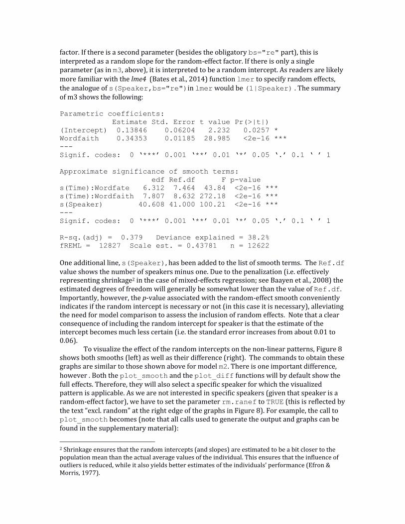
One additional line, s(Speaker), has been added to the list of smooth terms. The Ref.df value shows the number of speakers minus one. Due to the penalization (i.e. effectively representing shrinkage2 in the case of mixed-effects regression; see Baayen et al., 2008) the estimated degrees of freedom will generally be somewhat lower than the value of Ref.df. Importantly, however, the p-value associated with the random-effect smooth conveniently indicates if the random intercept is necessary or not (in this case it is necessary), alleviating the need for model comparison to assess the inclusion of random effects. Note that a clear consequence of including the random intercept for speaker is that the estimate of the intercept becomes much less certain (i.e. the standard error increases from about 0.01 to 0.06).
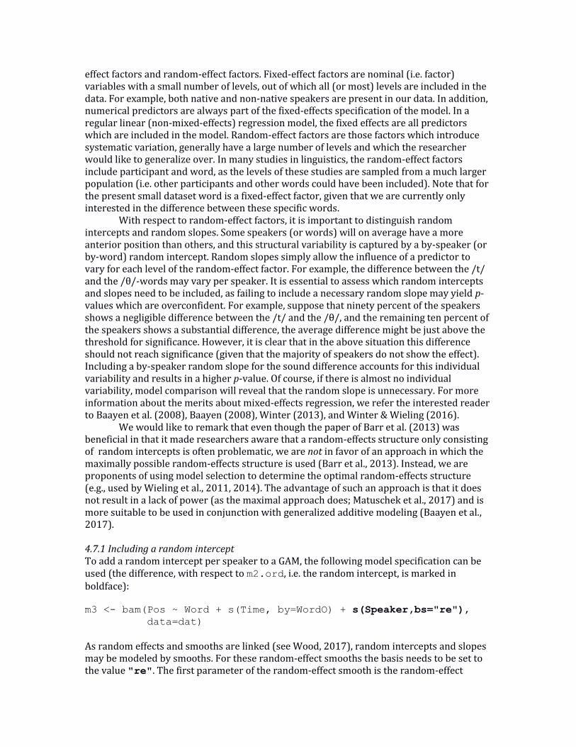
To visualize the effect of the random intercepts on the non-linear patterns, Figure 8 shows both smooths (left) as well as their difference (right). The commands to obtain these graphs are similar to those shown above for model m2. There is one important difference, however . Both the plot_smooth and the plot_diff functions will by default show the full effects. Therefore, they will also select a specific speaker for which the visualized pattern is applicable. As we are not interested in specific speakers (given that speaker is a random-effect factor), we have to set the parameter rm.ranef to TRUE (this is reflected by the text “excl. random” at the right edge of the graphs in Figure 8). For example, the call to plot_smooth becomes (note that all calls used to generate the output and graphs can be found in the supplementary material):
2 Shrinkage ensures that the random intercepts (and slopes) are estimated to be a bit closer to the population mean than the actual average values of the individual. This ensures that the influence of outliers is reduced, while it also yields better estimates of the individuals’ performance (Efron & Morris, 1977).
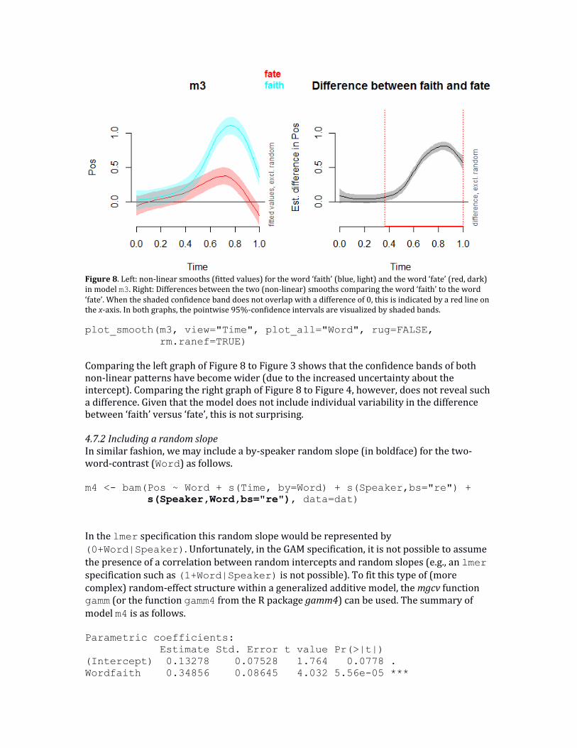
Figure 8. Left: non-linear smooths (fitted values) for the word ‘faith’ (blue, light) and the word ‘fate’ (red, dark) in model m3. Right: Differences between the two (non-linear) smooths comparing the word ‘faith’ to the word ‘fate’. When the shaded confidence band does not overlap with a difference of 0, this is indicated by a red line on the x-axis. In both graphs, the pointwise 95%-confidence intervals are visualized by shaded bands.
plot_smooth(m3, view="Time", plot_all="Word", rug=FALSE,
rm.ranef=TRUE)
Comparing the left graph of Figure 8 to Figure 3 shows that the confidence bands of both non-linear patterns have become wider (due to the increased uncertainty about the intercept). Comparing the right graph of Figure 8 to Figure 4, however, does not reveal such a difference. Given that the model does not include individual variability in the difference between ‘faith’ versus ‘fate’, this is not surprising. 4.7.2 Including a random slope In similar fashion, we may include a by-speaker random slope (in boldface) for the two-word-contrast (Word) as follows. m4 <- bam(Pos ~ Word + s(Time, by=Word) + s(Speaker,bs="re") +
s(Speaker,Word,bs="re"), data=dat)
In the lmer specification this random slope would be represented by (0+Word|Speaker). Unfortunately, in the GAM specification, it is not possible to assume
the presence of a correlation between random intercepts and random slopes (e.g., an lmer specification such as (1+Word|Speaker) is not possible). To fit this type of (more complex) random-effect structure within a generalized additive model, the mgcv function gamm (or the function gamm4 from the R package gamm4) can be used. The summary of
model m4 is as follows. Parametric coefficients:
Estimate Std. Error t value Pr(>|t|)
(Intercept) 0.13278 0.07528 1.764 0.0778 .
Wordfaith 0.34856 0.08645 4.032 5.56e-05 ***
---
Signif. codes: 0 ‘***’ 0.001 ‘**’ 0.01 ‘*’ 0.05 ‘.’ 0.1 ‘ ’ 1
Approximate significance of smooth terms:
edf Ref.df F p-value
s(Time):Wordfate 6.519 7.656 51.71 < 2e-16 ***
s(Time):Wordfaith 7.947 8.708 325.85 < 2e-16 ***
s(Speaker) 20.818 41.000 2029.09 0.00336 **
s(Speaker,Word) 60.177 82.000 958.37 0.00580 **
---
Signif. codes: 0 ‘***’ 0.001 ‘**’ 0.01 ‘*’ 0.05 ‘.’ 0.1 ‘ ’ 1
R-sq.(adj) = 0.485 Deviance explained = 48.9%
fREML = 11733 Scale est. = 0.36292 n = 12622
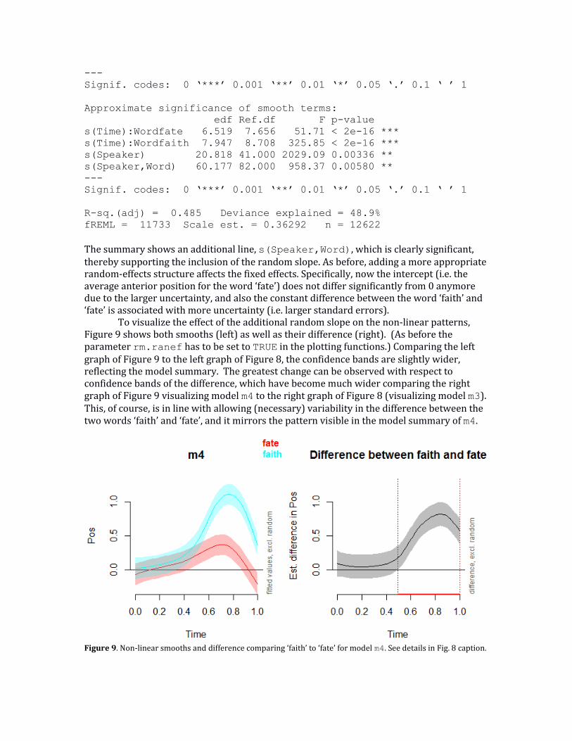
The summary shows an additional line, s(Speaker,Word), which is clearly significant, thereby supporting the inclusion of the random slope. As before, adding a more appropriate random-effects structure affects the fixed effects. Specifically, now the intercept (i.e. the average anterior position for the word ‘fate’) does not differ significantly from 0 anymore due to the larger uncertainty, and also the constant difference between the word ‘faith’ and ‘fate’ is associated with more uncertainty (i.e. larger standard errors). To visualize the effect of the additional random slope on the non-linear patterns, Figure 9 shows both smooths (left) as well as their difference (right). (As before the parameter rm.ranef has to be set to TRUE in the plotting functions.) Comparing the left graph of Figure 9 to the left graph of Figure 8, the confidence bands are slightly wider, reflecting the model summary. The greatest change can be observed with respect to confidence bands of the difference, which have become much wider comparing the right graph of Figure 9 visualizing model m4 to the right graph of Figure 8 (visualizing model m3). This, of course, is in line with allowing (necessary) variability in the difference between the two words ‘faith’ and ‘fate’, and it mirrors the pattern visible in the model summary of m4.
Figure 9. Non-linear smooths and difference comparing ‘faith’ to ‘fate’ for model m4. See details in Fig. 8 caption.
4.7.3 Including non-linear random effects While we are now able to model random intercepts and random slopes, our present model does not take individual variability in tongue movement patterns over time into account. Consequently, there is a need for a non-linear random effect. Within the GAM-framework, fortunately, this is possible. The following model specification illustrates how this can be achieved: m5 <- bam(Pos ~ Word + s(Time, by=Word) + s(Speaker,Word,bs="re")
+ s(Time,Speaker,bs="fs",m=1), data=dat)
In this model the random intercept part has been replaced by the smooth specification s(Time,Speaker,bs="fs",m=1). This is a so-called factor smooth (hence the "fs" basis) which models a (potentially) non-linear difference over time (the first parameter) with respect to the general time pattern for each of the speakers (the second parameter: the random-effect factor). (Note the different ordering compared to the random intercepts and slopes.) The final parameter, m, indicates the order of the non-linearity penalty. In this case it is set to 1, which means that the first derivative of the smooth (i.e. the speed) is penalized, rather than the, default, second derivative of the smooth (i.e. the acceleration). Effectively, this results in factor smooths which are penalized more than the other smooths. This, in turn, means that the estimated non-linear differences for the levels of the random-effect factor are assumed to be somewhat less ‘wiggly’ than their actual patterns. This reduced non-linearity therefore lines up nicely with the idea of shrinkage of the random effects (i.e. see footnote 2). Importantly, the factor smooths are not centered (i.e. they contain an intercept shift), and thereby the by-speaker random intercepts was dropped from the model specification. The summary of the model is shown below: Parametric coefficients:
Estimate Std. Error t value Pr(>|t|)
(Intercept) 0.11656 0.08909 1.308 0.191
Wordfaith 0.34888 0.08638 4.039 5.41e-05 ***
---
Signif. codes: 0 ‘***’ 0.001 ‘**’ 0.01 ‘*’ 0.05 ‘.’ 0.1 ‘ ’ 1
Approximate significance of smooth terms:
edf Ref.df F p-value
s(Time):Wordfate 5.757 6.485 8.694 6.71e-10 ***
s(Time):Wordfaith 7.717 8.347 25.918 < 2e-16 ***
s(Speaker,Word) 55.964 82.000 46.425 < 2e-16 ***
s(Time,Speaker) 295.198 377.000 925.716 1.69e-05 ***
---
Signif. codes: 0 ‘***’ 0.001 ‘**’ 0.01 ‘*’ 0.05 ‘.’ 0.1 ‘ ’ 1
R-sq.(adj) = 0.646 Deviance explained = 65.6%
fREML = 9755.7 Scale est. = 0.24974 n = 12622
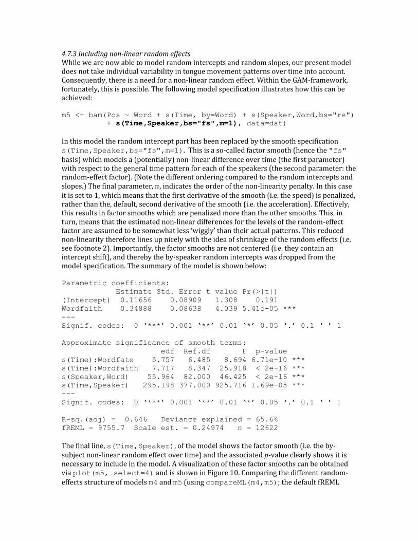
The final line, s(Time,Speaker), of the model shows the factor smooth (i.e. the by-subject non-linear random effect over time) and the associated p-value clearly shows it is necessary to include in the model. A visualization of these factor smooths can be obtained via plot(m5, select=4) and is shown in Figure 10. Comparing the different random-effects structure of models m4 and m5 (using compareML(m4,m5); the default fREML
estimation method now is appropriate as only random effects are compared) shows m5 is preferred over m4. Chi-square test of fREML scores
-----
Model Score Edf Chisq Df p.value Sig.
1 m4 11732.645 8
2 m5 9755.733 9 1976.912 1.000 < 2e-16 ***
AIC difference: 4453.17, model m5 has lower AIC.
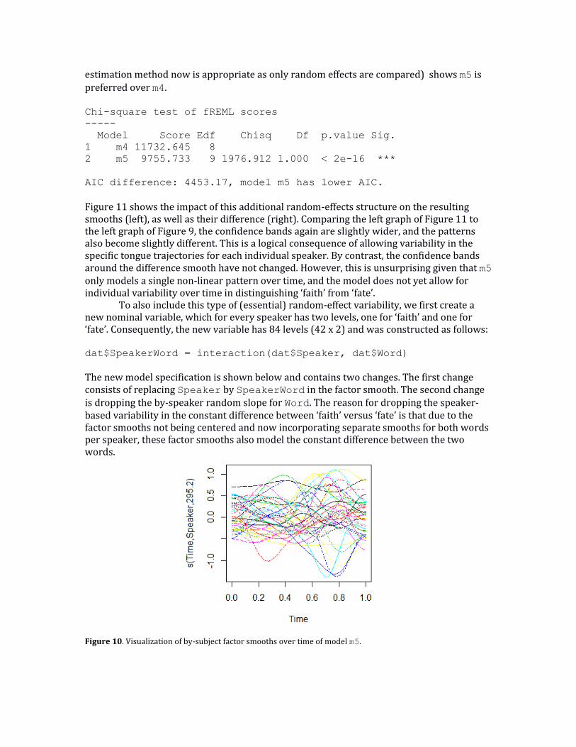
Figure 11 shows the impact of this additional random-effects structure on the resulting smooths (left), as well as their difference (right). Comparing the left graph of Figure 11 to the left graph of Figure 9, the confidence bands again are slightly wider, and the patterns also become slightly different. This is a logical consequence of allowing variability in the specific tongue trajectories for each individual speaker. By contrast, the confidence bands around the difference smooth have not changed. However, this is unsurprising given that m5 only models a single non-linear pattern over time, and the model does not yet allow for individual variability over time in distinguishing ‘faith’ from ‘fate’.
To also include this type of (essential) random-effect variability, we first create a new nominal variable, which for every speaker has two levels, one for ‘faith’ and one for ‘fate’. Consequently, the new variable has 84 levels (42 x 2) and was constructed as follows:
dat$SpeakerWord = interaction(dat$Speaker, dat$Word)
The new model specification is shown below and contains two changes. The first change consists of replacing Speaker by SpeakerWord in the factor smooth. The second change
is dropping the by-speaker random slope for Word. The reason for dropping the speaker-based variability in the constant difference between ‘faith’ versus ‘fate’ is that due to the factor smooths not being centered and now incorporating separate smooths for both words per speaker, these factor smooths also model the constant difference between the two words.
Figure 10. Visualization of by-subject factor smooths over time of model m5.
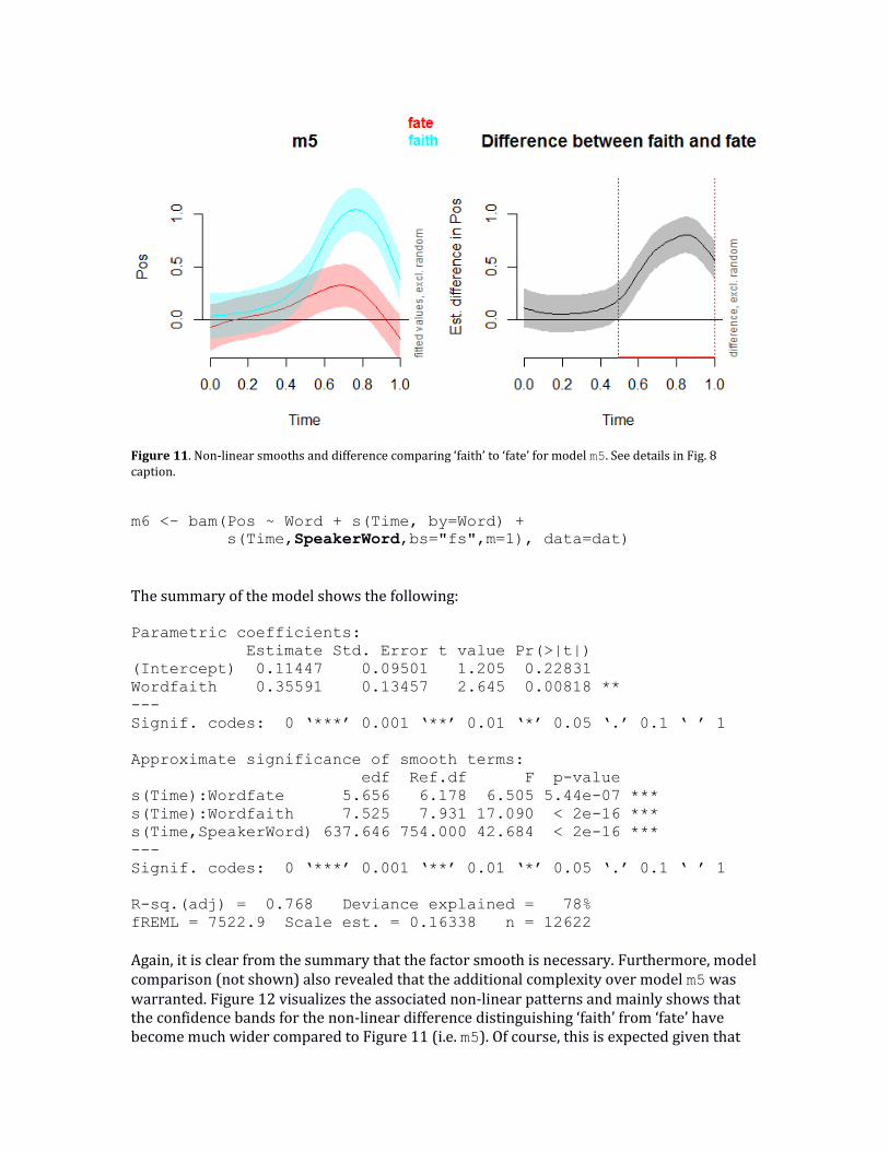
Figure 11. Non-linear smooths and difference comparing ‘faith’ to ‘fate’ for model m5. See details in Fig. 8 caption.
m6 <- bam(Pos ~ Word + s(Time, by=Word) +
s(Time,SpeakerWord,bs="fs",m=1), data=dat)
The summary of the model shows the following: Parametric coefficients:
Estimate Std. Error t value Pr(>|t|)
(Intercept) 0.11447 0.09501 1.205 0.22831
Wordfaith 0.35591 0.13457 2.645 0.00818 **
---
Signif. codes: 0 ‘***’ 0.001 ‘**’ 0.01 ‘*’ 0.05 ‘.’ 0.1 ‘ ’ 1
Approximate significance of smooth terms:
edf Ref.df F p-value
s(Time):Wordfate 5.656 6.178 6.505 5.44e-07 ***
s(Time):Wordfaith 7.525 7.931 17.090 < 2e-16 ***
s(Time,SpeakerWord) 637.646 754.000 42.684 < 2e-16 ***
---
Signif. codes: 0 ‘***’ 0.001 ‘**’ 0.01 ‘*’ 0.05 ‘.’ 0.1 ‘ ’ 1
R-sq.(adj) = 0.768 Deviance explained = 78%
fREML = 7522.9 Scale est. = 0.16338 n = 12622
Again, it is clear from the summary that the factor smooth is necessary. Furthermore, model comparison (not shown) also revealed that the additional complexity over model m5 was warranted. Figure 12 visualizes the associated non-linear patterns and mainly shows that the confidence bands for the non-linear difference distinguishing ‘faith’ from ‘fate’ have become much wider compared to Figure 11 (i.e. m5). Of course, this is expected given that
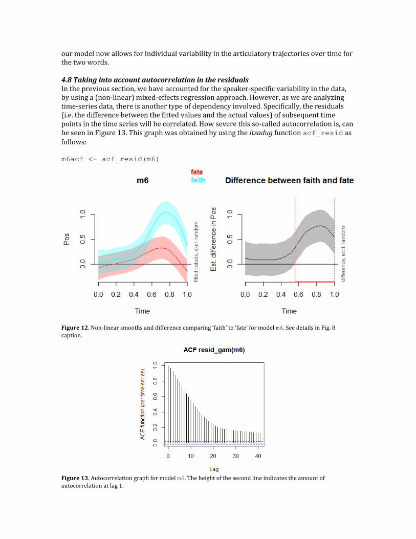
our model now allows for individual variability in the articulatory trajectories over time for the two words. 4.8 Taking into account autocorrelation in the residuals In the previous section, we have accounted for the speaker-specific variability in the data, by using a (non-linear) mixed-effects regression approach. However, as we are analyzing time-series data, there is another type of dependency involved. Specifically, the residuals (i.e. the difference between the fitted values and the actual values) of subsequent time points in the time series will be correlated. How severe this so-called autocorrelation is, can be seen in Figure 13. This graph was obtained by using the itsadug function acf_resid as follows: m6acf <- acf_resid(m6)
Figure 12. Non-linear smooths and difference comparing ‘faith’ to ‘fate’ for model m6. See details in Fig. 8 caption.
Figure 13. Autocorrelation graph for model m6. The height of the second line indicates the amount of autocorrelation at lag 1.
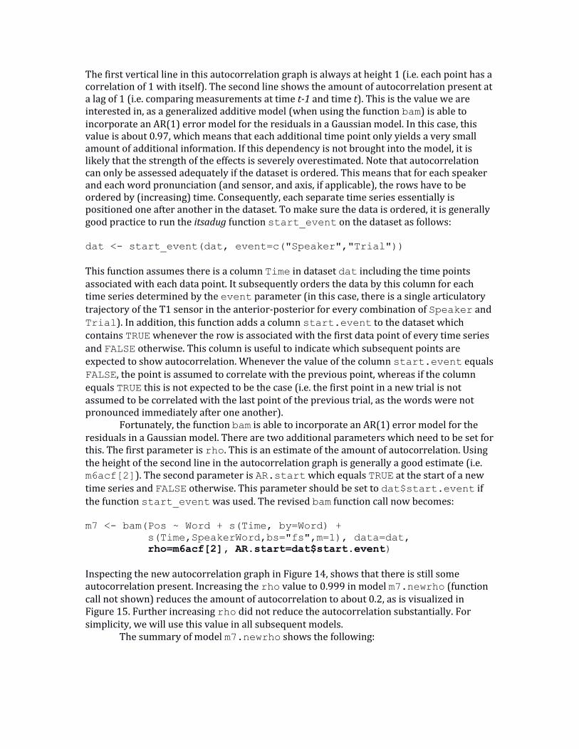
The first vertical line in this autocorrelation graph is always at height 1 (i.e. each point has a correlation of 1 with itself). The second line shows the amount of autocorrelation present at a lag of 1 (i.e. comparing measurements at time t-1 and time t). This is the value we are interested in, as a generalized additive model (when using the function bam) is able to incorporate an AR(1) error model for the residuals in a Gaussian model. In this case, this value is about 0.97, which means that each additional time point only yields a very small amount of additional information. If this dependency is not brought into the model, it is likely that the strength of the effects is severely overestimated. Note that autocorrelation can only be assessed adequately if the dataset is ordered. This means that for each speaker and each word pronunciation (and sensor, and axis, if applicable), the rows have to be ordered by (increasing) time. Consequently, each separate time series essentially is positioned one after another in the dataset. To make sure the data is ordered, it is generally good practice to run the itsadug function start_event on the dataset as follows: dat <- start_event(dat, event=c("Speaker","Trial"))
This function assumes there is a column Time in dataset dat including the time points associated with each data point. It subsequently orders the data by this column for each time series determined by the event parameter (in this case, there is a single articulatory trajectory of the T1 sensor in the anterior-posterior for every combination of Speaker and
Trial). In addition, this function adds a column start.event to the dataset which contains TRUE whenever the row is associated with the first data point of every time series and FALSE otherwise. This column is useful to indicate which subsequent points are expected to show autocorrelation. Whenever the value of the column start.event equals FALSE, the point is assumed to correlate with the previous point, whereas if the column
equals TRUE this is not expected to be the case (i.e. the first point in a new trial is not assumed to be correlated with the last point of the previous trial, as the words were not pronounced immediately after one another).
Fortunately, the function bam is able to incorporate an AR(1) error model for the residuals in a Gaussian model. There are two additional parameters which need to be set for this. The first parameter is rho. This is an estimate of the amount of autocorrelation. Using the height of the second line in the autocorrelation graph is generally a good estimate (i.e. m6acf[2]). The second parameter is AR.start which equals TRUE at the start of a new
time series and FALSE otherwise. This parameter should be set to dat$start.event if
the function start_event was used. The revised bam function call now becomes: m7 <- bam(Pos ~ Word + s(Time, by=Word) +
s(Time,SpeakerWord,bs="fs",m=1), data=dat,
rho=m6acf[2], AR.start=dat$start.event)
Inspecting the new autocorrelation graph in Figure 14, shows that there is still some autocorrelation present. Increasing the rho value to 0.999 in model m7.newrho (function call not shown) reduces the amount of autocorrelation to about 0.2, as is visualized in Figure 15. Further increasing rho did not reduce the autocorrelation substantially. For simplicity, we will use this value in all subsequent models.
The summary of model m7.newrho shows the following:
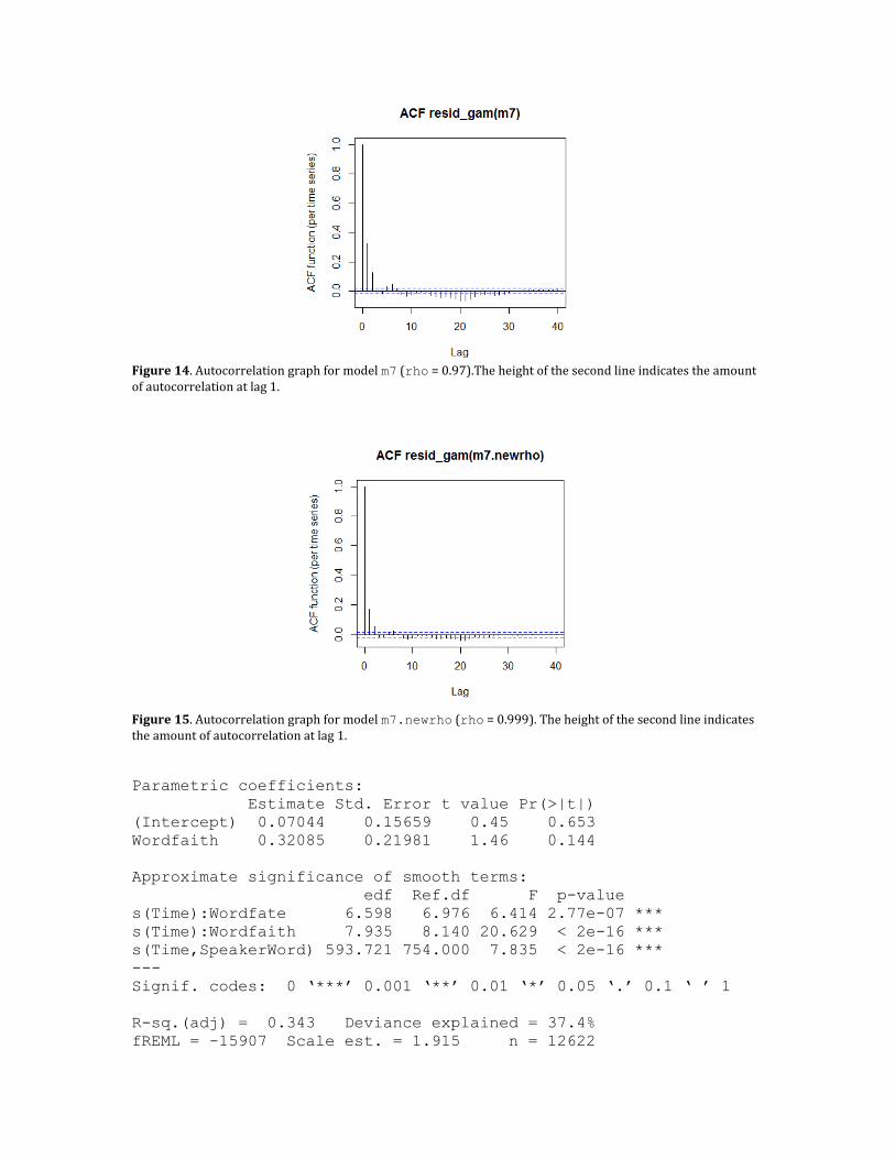
Figure 14. Autocorrelation graph for model m7 (rho = 0.97).The height of the second line indicates the amount of autocorrelation at lag 1.
Figure 15. Autocorrelation graph for model m7.newrho (rho = 0.999). The height of the second line indicates the amount of autocorrelation at lag 1.
Parametric coefficients:
Estimate Std. Error t value Pr(>|t|)
(Intercept) 0.07044 0.15659 0.45 0.653
Wordfaith 0.32085 0.21981 1.46 0.144
Approximate significance of smooth terms:
edf Ref.df F p-value
s(Time):Wordfate 6.598 6.976 6.414 2.77e-07 ***
s(Time):Wordfaith 7.935 8.140 20.629 < 2e-16 ***
s(Time,SpeakerWord) 593.721 754.000 7.835 < 2e-16 ***
---
Signif. codes: 0 ‘***’ 0.001 ‘**’ 0.01 ‘*’ 0.05 ‘.’ 0.1 ‘ ’ 1
R-sq.(adj) = 0.343 Deviance explained = 37.4%
fREML = -15907 Scale est. = 1.915 n = 12622
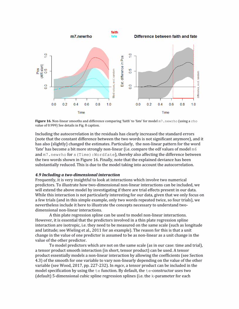
Figure 16. Non-linear smooths and difference comparing ‘faith’ to ‘fate’ for model m7.newrho (using a rho value of 0.999) See details in Fig. 8 caption.
Including the autocorrelation in the residuals has clearly increased the standard errors (note that the constant difference between the two words is not significant anymore), and it has also (slightly) changed the estimates. Particularly, the non-linear pattern for the word ‘fate’ has become a bit more strongly non-linear (i.e. compare the edf values of model m6 and m7.newrho for s(Time):Wordfate), thereby also affecting the difference between the two words shown in Figure 16. Finally, note that the explained deviance has been substantially reduced. This is due to the model taking into account the autocorrelation. 4.9 Including a two-dimensional interaction Frequently, it is very insightful to look at interactions which involve two numerical predictors. To illustrate how two-dimensional non-linear interactions can be included, we will extend the above model by investigating if there are trial effects present in our data. While this interaction is not particularly interesting for our data, given that we only focus on a few trials (and in this simple example, only two words repeated twice, so four trials), we nevertheless include it here to illustrate the concepts necessary to understand two-dimensional non-linear interactions. A thin plate regression spline can be used to model non-linear interactions. However, it is essential that the predictors involved in a thin plate regression spline interaction are isotropic, i.e. they need to be measured on the same scale (such as longitude and latitude; see Wieling et al., 2011 for an example). The reason for this is that a unit change in the value of one predictor is assumed to be as non-linear as a unit change in the value of the other predictor.
To model predictors which are not on the same scale (as in our case: time and trial), a tensor product smooth interaction (in short, tensor product) can be used. A tensor product essentially models a non-linear interaction by allowing the coefficients (see Section 4.3) of the smooth for one variable to vary non-linearly depending on the value of the other variable (see Wood, 2017, pp. 227-232). In mgcv, a tensor product can be included in the model specification by using the te function. By default, the te-constructor uses two (default) 5-dimensional cubic spline regression splines (i.e. the k-parameter for each
variable is limited to 5: k=c(5,5); the sequence is equal to the order of the variables in the tensor product). Extending model m7.newrho to include a two dimensional interaction between Time and Trial thus results in the following function call:
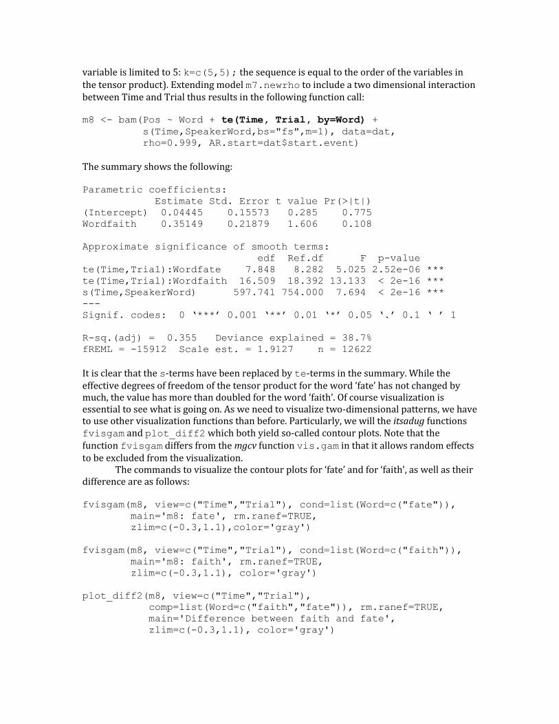
m8 <- bam(Pos ~ Word + te(Time, Trial, by=Word) +
s(Time,SpeakerWord,bs="fs",m=1), data=dat,
rho=0.999, AR.start=dat$start.event)
The summary shows the following: Parametric coefficients:
Estimate Std. Error t value Pr(>|t|)
(Intercept) 0.04445 0.15573 0.285 0.775
Wordfaith 0.35149 0.21879 1.606 0.108
Approximate significance of smooth terms:
edf Ref.df F p-value
te(Time,Trial):Wordfate 7.848 8.282 5.025 2.52e-06 ***
te(Time,Trial):Wordfaith 16.509 18.392 13.133 < 2e-16 ***
s(Time,SpeakerWord) 597.741 754.000 7.694 < 2e-16 ***
---
Signif. codes: 0 ‘***’ 0.001 ‘**’ 0.01 ‘*’ 0.05 ‘.’ 0.1 ‘ ’ 1
R-sq.(adj) = 0.355 Deviance explained = 38.7%
fREML = -15912 Scale est. = 1.9127 n = 12622 It is clear that the s-terms have been replaced by te-terms in the summary. While the effective degrees of freedom of the tensor product for the word ‘fate’ has not changed by much, the value has more than doubled for the word ‘faith’. Of course visualization is essential to see what is going on. As we need to visualize two-dimensional patterns, we have to use other visualization functions than before. Particularly, we will the itsadug functions fvisgam and plot_diff2 which both yield so-called contour plots. Note that the function fvisgam differs from the mgcv function vis.gam in that it allows random effects to be excluded from the visualization. The commands to visualize the contour plots for ‘fate’ and for ‘faith’, as well as their difference are as follows: fvisgam(m8, view=c("Time","Trial"), cond=list(Word=c("fate")),
main='m8: fate', rm.ranef=TRUE,
zlim=c(-0.3,1.1),color='gray')
fvisgam(m8, view=c("Time","Trial"), cond=list(Word=c("faith")),
main='m8: faith', rm.ranef=TRUE,
zlim=c(-0.3,1.1), color='gray')
plot_diff2(m8, view=c("Time","Trial"),
comp=list(Word=c("faith","fate")), rm.ranef=TRUE,
main='Difference between faith and fate',
zlim=c(-0.3,1.1), color='gray')
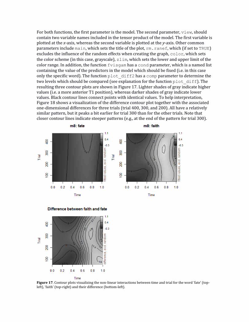
For both functions, the first parameter is the model. The second parameter, view, should contain two variable names included in the tensor product of the model. The first variable is plotted at the x-axis, whereas the second variable is plotted at the y-axis. Other common parameters include main, which sets the title of the plot, rm.ranef, which (if set to TRUE) excludes the influence of the random effects when creating the graph, color, which sets
the color scheme (in this case, grayscale), zlim, which sets the lower and upper limit of the color range. In addition, the function fvisgam has a cond parameter, which is a named list containing the value of the predictors in the model which should be fixed (i.e. in this case only the specific word). The function plot_diff2 has a comp parameter to determine the two levels which should be compared (see explanation for the function plot_diff). The resulting three contour plots are shown in Figure 17. Lighter shades of gray indicate higher values (i.e. a more anterior T1 position), whereas darker shades of gray indicate lower values. Black contour lines connect points with identical values. To help interpretation, Figure 18 shows a visualization of the difference contour plot together with the associated one-dimensional differences for three trials (trial 400, 300, and 200). All have a relatively similar pattern, but it peaks a bit earlier for trial 300 than for the other trials. Note that closer contour lines indicate steeper patterns (e.g., at the end of the pattern for trial 300).
Figure 17. Contour plots visualizing the non-linear interactions between time and trial for the word ‘fate’ (top-left), ‘faith’ (top-right) and their difference (bottom-left).
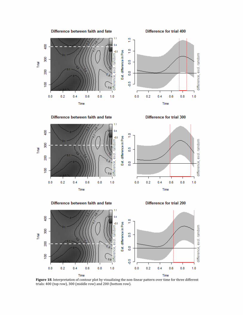
Figure 18. Interpretation of contour plot by visualizing the non-linear pattern over time for three different trials: 400 (top row), 300 (middle row) and 200 (bottom row).
The two-dimensional tensor product of time and trial consists of three parts: an effect over time, an effect over trial, and the pure interaction between the two. Inspecting Figure 17 and 18, it does not appear there is a very large influence of trial. Consequently, it makes sense to see whether an effect of trial would need to be included at all. For this reason, it is useful to decompose the tensor product. While we already have seen how to model one-dimensional smooths, to model a pure interaction term, we need to introduce a new constructor, ti. This constructor, with identical syntax to the te-constructor, models the pure interaction between its contained variables. The specification of the model (m8.dc) of the decomposed tensor product is as follows: m8.dc <- bam(Pos ~ Word + s(Time, by=Word) + s(Trial, by=Word) +
ti(Time, Trial, by=Word) +
s(Time,SpeakerWord,bs="fs",m=1), data=dat,
rho=0.999, AR.start=dat$start.event)
The summary of the model is as follows: Parametric coefficients:
Estimate Std. Error t value Pr(>|t|)
(Intercept) 0.06768 0.15665 0.432 0.666
Wordfaith 0.32746 0.21989 1.489 0.136
Approximate significance of smooth terms:
edf Ref.df F p-value
s(Time):Wordfate 6.603 6.980 6.420 2.55e-07 ***
s(Time):Wordfaith 7.936 8.140 20.807 < 2e-16 ***
s(Trial):Wordfate 1.000 1.000 0.060 0.806
s(Trial):Wordfaith 1.000 1.000 0.023 0.880
ti(Time,Trial):Wordfate 1.001 1.002 0.132 0.716
ti(Time,Trial):Wordfaith 9.141 11.335 4.754 1.91e-07 ***
s(Time,SpeakerWord) 593.372 754.000 7.730 < 2e-16 ***
---
Signif. codes: 0 ‘***’ 0.001 ‘**’ 0.01 ‘*’ 0.05 ‘.’ 0.1 ‘ ’ 1
R-sq.(adj) = 0.35 Deviance explained = 38.2%
fREML = -15923 Scale est. = 1.9067 n = 12622
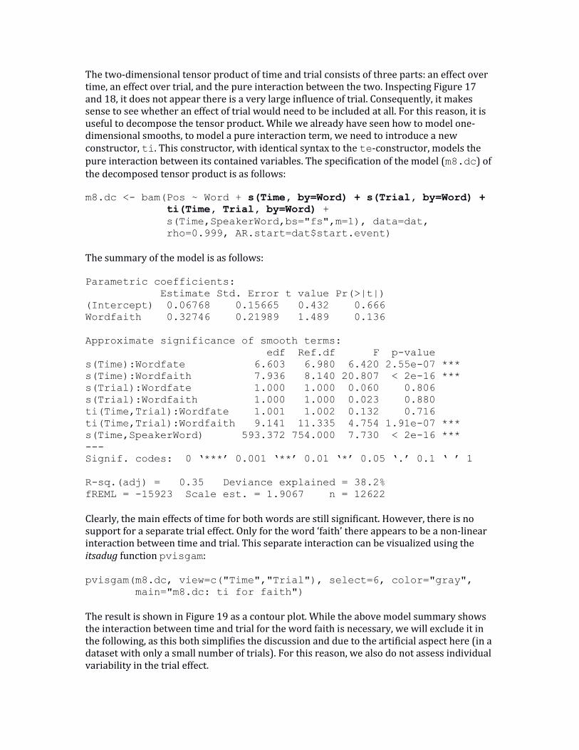
Clearly, the main effects of time for both words are still significant. However, there is no support for a separate trial effect. Only for the word ‘faith’ there appears to be a non-linear interaction between time and trial. This separate interaction can be visualized using the itsadug function pvisgam: pvisgam(m8.dc, view=c("Time","Trial"), select=6, color="gray",
main="m8.dc: ti for faith")
The result is shown in Figure 19 as a contour plot. While the above model summary shows the interaction between time and trial for the word faith is necessary, we will exclude it in the following, as this both simplifies the discussion and due to the artificial aspect here (in a dataset with only a small number of trials). For this reason, we also do not assess individual variability in the trial effect.
Figure 19. Pure tensor product interaction between time and trial for model m8.dc.
4.10 Including the language difference While we only considered the difference between the two words in the models above, a more interesting question is how this difference varies depending on the language of the speaker. Consequently, we create a new variable which is the interaction between Word and Lang (i.e. having four levels, the words ‘fate’ and ‘faith’ for both English and Dutch speakers): dat$WordLang <- interaction(dat$Word, dat$Lang) We now use this new variable in our model instead of Word: m9 <- bam(Pos ~ WordLang + s(Time, by=WordLang) +
s(Time,SpeakerWord,bs="fs",m=1), data=dat,
rho=0.999, AR.start=dat$start.event)
The summary of the model now shows three contrasts with respect to the intercept (in this case the reference level is the word ‘fate’ for the native English speakers) and four smooths, one for each level of the new nominal variable. Parametric coefficients:
Estimate Std. Error t value Pr(>|t|)
(Intercept) 0.03183 0.21184 0.150 0.881
WordLangfaith.EN 0.42836 0.30009 1.427 0.153
WordLangfate.NL 0.07542 0.31370 0.240 0.810
WordLangfaith.NL 0.29328 0.30770 0.953 0.341
Approximate significance of smooth terms:
edf Ref.df F p-value
s(Time):WordLangfate.EN 5.552 5.999 3.775 0.000924 ***
s(Time):WordLangfaith.EN 7.509 7.790 14.554 < 2e-16 ***
s(Time):WordLangfate.NL 6.967 7.316 7.029 2.99e-06 ***
s(Time):WordLangfaith.NL 7.369 7.650 4.080 0.000182 ***
s(Time,SpeakerWord) 583.691 752.000 7.382 < 2e-16 ***
---
Signif. codes: 0 ‘***’ 0.001 ‘**’ 0.01 ‘*’ 0.05 ‘.’ 0.1 ‘ ’ 1
R-sq.(adj) = 0.347 Deviance explained = 37.9%
fREML = -15909 Scale est. = 1.9134 n = 12622
The top row of Figure 20 shows the individual smooths (top-left) for the English speakers as well as the difference (top-right) which shows a clear significant pattern. The bottom row shows the same graphs for the Dutch speakers, with a much smaller difference between the two words. While it seems the difference between the two words for the Dutch speakers is not necessary, we have to assess this formally. For this reason, we re-specify the model using ordered factors. As we want to evaluate the difference between ‘faith’ and ‘fate’ for both the English and Dutch speakers, separately, we create two reference levels via s(Time,by=Lang) + Lang. We then create two separate ordered factors. One factor
(ENFaithO) is set to "TRUE" whenever the word equals ‘faith’ and the language is English and "FALSE" otherwise, whereas the other factor (NLFaithO) is set to "TRUE" whenever the word equals ‘faith’ and the native language is Dutch and "FALSE" otherwise. The complete specification, including the creation of the two ordered factors is as follows: dat$ENFaithO <- as.ordered(dat$Lang == "EN" &
dat$Word == "faith")
contrasts(dat$ENFaithO) <- "contr.treatment"
dat$NLFaithO <- as.ordered(dat$Lang == "NL" &
dat$Word == "faith")
contrasts(dat$NLFaithO) <- "contr.treatment"
m9.ord <- bam(Pos ~ Lang + ENFaithO + NLFaithO +
s(Time,by=Lang) + s(Time,by=ENFaithO) +
s(Time,by=NLFaithO) +
s(Time,SpeakerWord,bs="fs",m=1), data=dat,
rho=0.999, AR.start=dat$start.event)
The summary of this model shows the following: Parametric coefficients:
Estimate Std. Error t value Pr(>|t|)
(Intercept) 0.02804 0.21151 0.133 0.895
LangNL 0.07205 0.31305 0.230 0.818
ENFaithOTRUE 0.43838 0.29932 1.465 0.143
NLFaithOTRUE 0.22638 0.32064 0.706 0.480
Approximate significance of smooth terms:
edf Ref.df F p-value
s(Time):LangEN 5.873 6.271 3.995 0.000444 ***
s(Time):LangNL 6.693 7.038 5.740 2.76e-06 ***
s(Time):ENFaithOTRUE 6.764 7.098 5.219 8.55e-06 ***
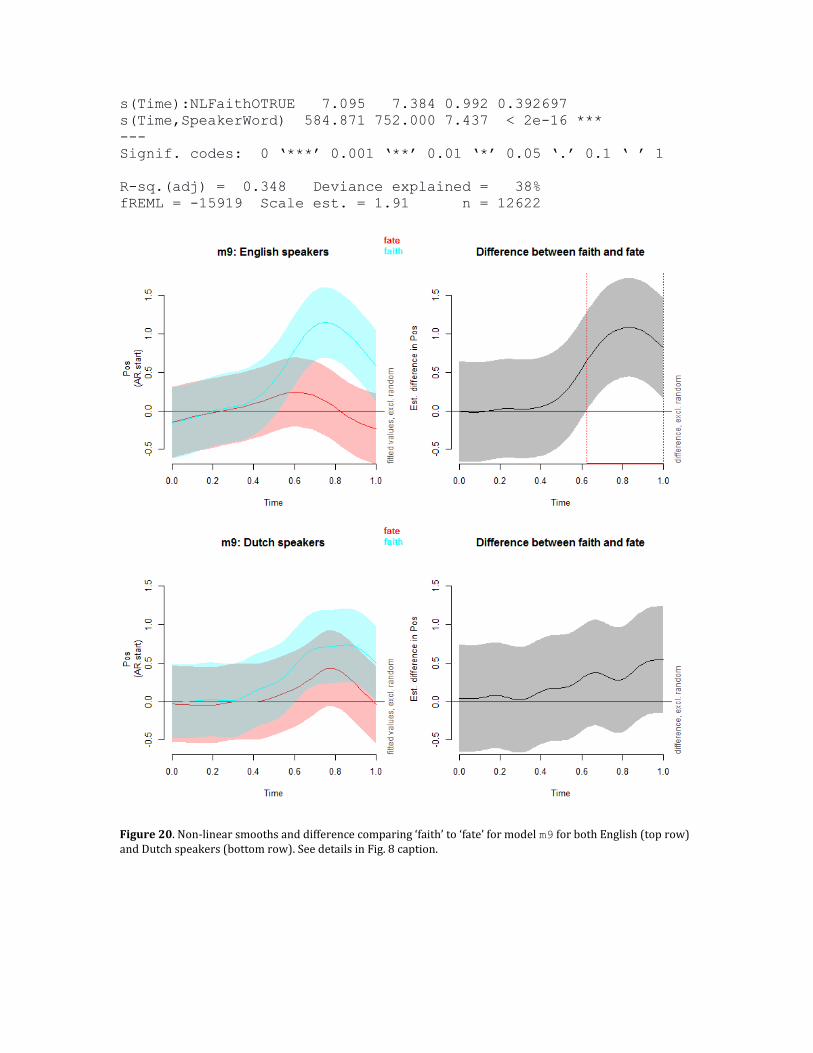
s(Time):NLFaithOTRUE 7.095 7.384 0.992 0.392697
s(Time,SpeakerWord) 584.871 752.000 7.437 < 2e-16 ***
---
Signif. codes: 0 ‘***’ 0.001 ‘**’ 0.01 ‘*’ 0.05 ‘.’ 0.1 ‘ ’ 1
R-sq.(adj) = 0.348 Deviance explained = 38%
fREML = -15919 Scale est. = 1.91 n = 12622
Figure 20. Non-linear smooths and difference comparing ‘faith’ to ‘fate’ for model m9 for both English (top row) and Dutch speakers (bottom row). See details in Fig. 8 caption.
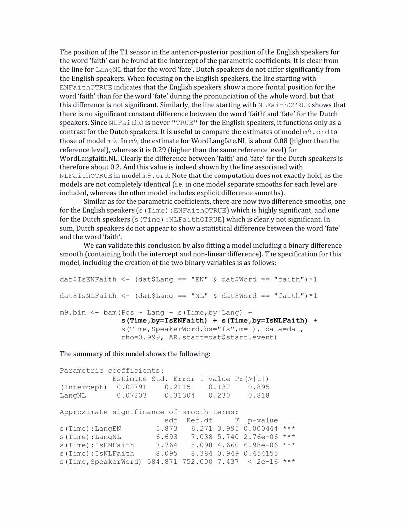
The position of the T1 sensor in the anterior-posterior position of the English speakers for the word ‘faith’ can be found at the intercept of the parametric coefficients. It is clear from the line for LangNL that for the word ‘fate’, Dutch speakers do not differ significantly from the English speakers. When focusing on the English speakers, the line starting with ENFaithOTRUE indicates that the English speakers show a more frontal position for the word ‘faith’ than for the word ‘fate’ during the pronunciation of the whole word, but that this difference is not significant. Similarly, the line starting with NLFaithOTRUE shows that there is no significant constant difference between the word ‘faith’ and ‘fate’ for the Dutch speakers. Since NLFaithO is never "TRUE" for the English speakers, it functions only as a contrast for the Dutch speakers. It is useful to compare the estimates of model m9.ord to those of model m9. In m9, the estimate for WordLangfate.NL is about 0.08 (higher than the reference level), whereas it is 0.29 (higher than the same reference level) for WordLangfaith.NL. Clearly the difference between ‘faith’ and ‘fate’ for the Dutch speakers is therefore about 0.2. And this value is indeed shown by the line associated with NLFaithOTRUE in model m9.ord. Note that the computation does not exactly hold, as the models are not completely identical (i.e. in one model separate smooths for each level are included, whereas the other model includes explicit difference smooths). Similar as for the parametric coefficients, there are now two difference smooths, one for the English speakers (s(Time):ENFaithOTRUE) which is highly significant, and one for the Dutch speakers (s(Time):NLFaithOTRUE) which is clearly not significant. In sum, Dutch speakers do not appear to show a statistical difference between the word ‘fate’ and the word ‘faith’. We can validate this conclusion by also fitting a model including a binary difference smooth (containing both the intercept and non-linear difference). The specification for this model, including the creation of the two binary variables is as follows: dat$IsENFaith <- (dat$Lang == "EN" & dat$Word == "faith")*1
dat$IsNLFaith <- (dat$Lang == "NL" & dat$Word == "faith")*1
m9.bin <- bam(Pos ~ Lang + s(Time,by=Lang) +
s(Time,by=IsENFaith) + s(Time,by=IsNLFaith) +
s(Time,SpeakerWord,bs="fs",m=1), data=dat,
rho=0.999, AR.start=dat$start.event)
The summary of this model shows the following: Parametric coefficients:
Estimate Std. Error t value Pr(>|t|)
(Intercept) 0.02791 0.21151 0.132 0.895
LangNL 0.07203 0.31304 0.230 0.818
Approximate significance of smooth terms:
edf Ref.df F p-value
s(Time):LangEN 5.873 6.271 3.995 0.000444 ***
s(Time):LangNL 6.693 7.038 5.740 2.76e-06 ***
s(Time):IsENFaith 7.764 8.098 4.660 6.98e-06 ***
s(Time):IsNLFaith 8.095 8.384 0.949 0.454155
s(Time,SpeakerWord) 584.871 752.000 7.437 < 2e-16 ***
---
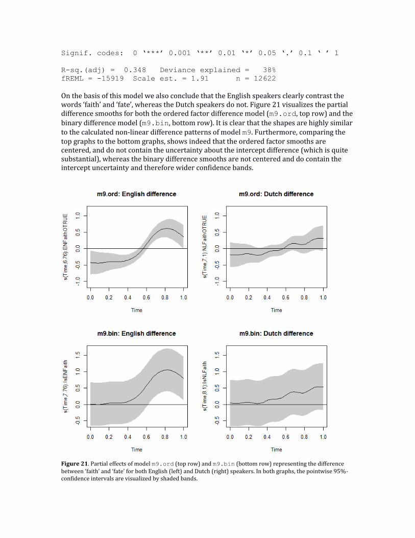
Signif. codes: 0 ‘***’ 0.001 ‘**’ 0.01 ‘*’ 0.05 ‘.’ 0.1 ‘ ’ 1
R-sq.(adj) = 0.348 Deviance explained = 38%
fREML = -15919 Scale est. = 1.91 n = 12622
On the basis of this model we also conclude that the English speakers clearly contrast the words ‘faith’ and ‘fate’, whereas the Dutch speakers do not. Figure 21 visualizes the partial difference smooths for both the ordered factor difference model (m9.ord, top row) and the binary difference model (m9.bin, bottom row). It is clear that the shapes are highly similar to the calculated non-linear difference patterns of model m9. Furthermore, comparing the top graphs to the bottom graphs, shows indeed that the ordered factor smooths are centered, and do not contain the uncertainty about the intercept difference (which is quite substantial), whereas the binary difference smooths are not centered and do contain the intercept uncertainty and therefore wider confidence bands.
Figure 21. Partial effects of model m9.ord (top row) and m9.bin (bottom row) representing the difference between ‘faith’ and ‘fate’ for both English (left) and Dutch (right) speakers. In both graphs, the pointwise 95%-confidence intervals are visualized by shaded bands.
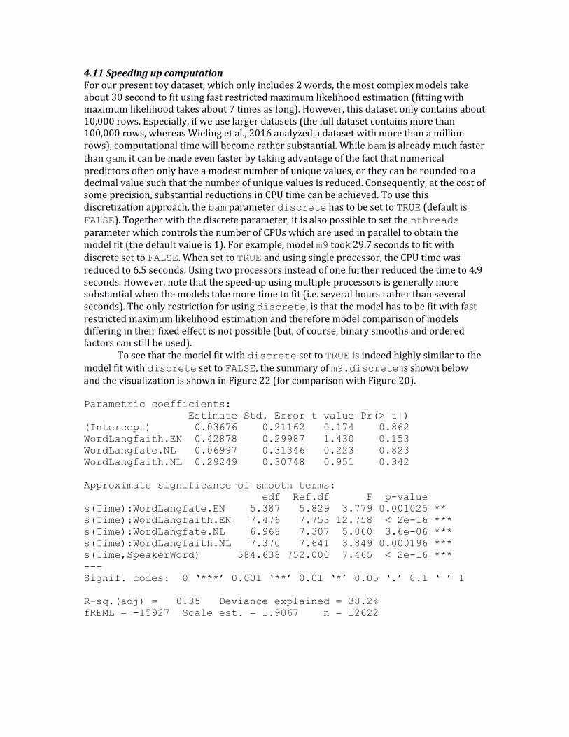
4.11 Speeding up computation For our present toy dataset, which only includes 2 words, the most complex models take about 30 second to fit using fast restricted maximum likelihood estimation (fitting with maximum likelihood takes about 7 times as long). However, this dataset only contains about 10,000 rows. Especially, if we use larger datasets (the full dataset contains more than 100,000 rows, whereas Wieling et al., 2016 analyzed a dataset with more than a million rows), computational time will become rather substantial. While bam is already much faster than gam, it can be made even faster by taking advantage of the fact that numerical predictors often only have a modest number of unique values, or they can be rounded to a decimal value such that the number of unique values is reduced. Consequently, at the cost of some precision, substantial reductions in CPU time can be achieved. To use this discretization approach, the bam parameter discrete has to be set to TRUE (default is FALSE). Together with the discrete parameter, it is also possible to set the nthreads parameter which controls the number of CPUs which are used in parallel to obtain the model fit (the default value is 1). For example, model m9 took 29.7 seconds to fit with discrete set to FALSE. When set to TRUE and using single processor, the CPU time was reduced to 6.5 seconds. Using two processors instead of one further reduced the time to 4.9 seconds. However, note that the speed-up using multiple processors is generally more substantial when the models take more time to fit (i.e. several hours rather than several seconds). The only restriction for using discrete, is that the model has to be fit with fast restricted maximum likelihood estimation and therefore model comparison of models differing in their fixed effect is not possible (but, of course, binary smooths and ordered factors can still be used). To see that the model fit with discrete set to TRUE is indeed highly similar to the model fit with discrete set to FALSE, the summary of m9.discrete is shown below and the visualization is shown in Figure 22 (for comparison with Figure 20). Parametric coefficients:
Estimate Std. Error t value Pr(>|t|)
(Intercept) 0.03676 0.21162 0.174 0.862
WordLangfaith.EN 0.42878 0.29987 1.430 0.153
WordLangfate.NL 0.06997 0.31346 0.223 0.823
WordLangfaith.NL 0.29249 0.30748 0.951 0.342
Approximate significance of smooth terms:
edf Ref.df F p-value
s(Time):WordLangfate.EN 5.387 5.829 3.779 0.001025 **
s(Time):WordLangfaith.EN 7.476 7.753 12.758 < 2e-16 ***
s(Time):WordLangfate.NL 6.968 7.307 5.060 3.6e-06 ***
s(Time):WordLangfaith.NL 7.370 7.641 3.849 0.000196 ***
s(Time,SpeakerWord) 584.638 752.000 7.465 < 2e-16 ***
---
Signif. codes: 0 ‘***’ 0.001 ‘**’ 0.01 ‘*’ 0.05 ‘.’ 0.1 ‘ ’ 1
R-sq.(adj) = 0.35 Deviance explained = 38.2%
fREML = -15927 Scale est. = 1.9067 n = 12622
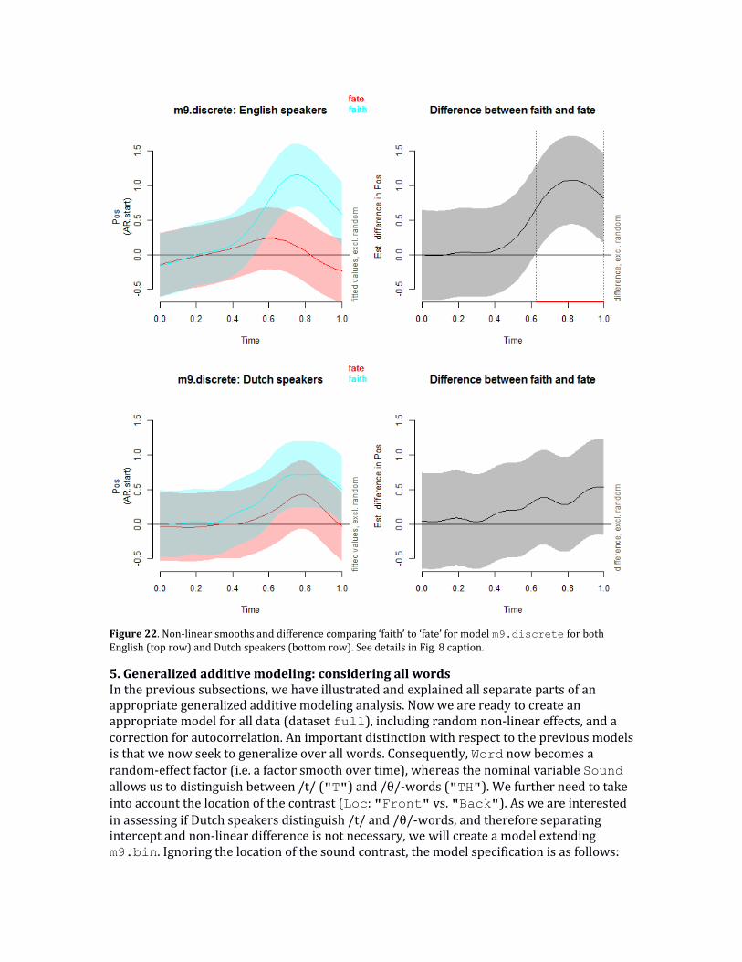
Figure 22. Non-linear smooths and difference comparing ‘faith’ to ‘fate’ for model m9.discrete for both English (top row) and Dutch speakers (bottom row). See details in Fig. 8 caption.
5. Generalized additive modeling: considering all words In the previous subsections, we have illustrated and explained all separate parts of an appropriate generalized additive modeling analysis. Now we are ready to create an appropriate model for all data (dataset full), including random non-linear effects, and a correction for autocorrelation. An important distinction with respect to the previous models is that we now seek to generalize over all words. Consequently, Word now becomes a random-effect factor (i.e. a factor smooth over time), whereas the nominal variable Sound allows us to distinguish between /t/ ("T") and /θ/-words ("TH"). We further need to take into account the location of the contrast (Loc: "Front" vs. "Back"). As we are interested
in assessing if Dutch speakers distinguish /t/ and /θ/-words, and therefore separating intercept and non-linear difference is not necessary, we will create a model extending m9.bin. Ignoring the location of the sound contrast, the model specification is as follows:
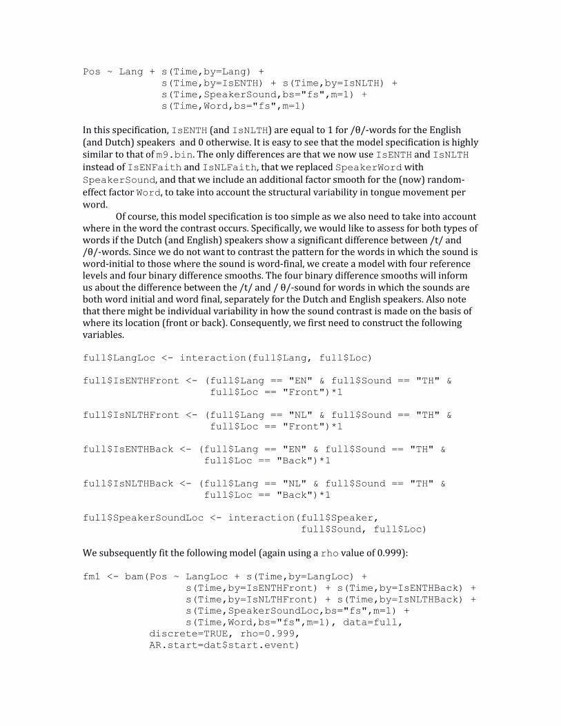
Pos ~ Lang + s(Time,by=Lang) +
s(Time,by=IsENTH) + s(Time,by=IsNLTH) +
s(Time,SpeakerSound,bs="fs",m=1) +
s(Time,Word,bs="fs",m=1) In this specification, IsENTH (and IsNLTH) are equal to 1 for /θ/-words for the English (and Dutch) speakers and 0 otherwise. It is easy to see that the model specification is highly similar to that of m9.bin. The only differences are that we now use IsENTH and IsNLTH
instead of IsENFaith and IsNLFaith, that we replaced SpeakerWord with SpeakerSound, and that we include an additional factor smooth for the (now) random-effect factor Word, to take into account the structural variability in tongue movement per word.
Of course, this model specification is too simple as we also need to take into account where in the word the contrast occurs. Specifically, we would like to assess for both types of words if the Dutch (and English) speakers show a significant difference between /t/ and /θ/-words. Since we do not want to contrast the pattern for the words in which the sound is word-initial to those where the sound is word-final, we create a model with four reference levels and four binary difference smooths. The four binary difference smooths will inform us about the difference between the /t/ and / θ/-sound for words in which the sounds are both word initial and word final, separately for the Dutch and English speakers. Also note that there might be individual variability in how the sound contrast is made on the basis of where its location (front or back). Consequently, we first need to construct the following variables. full$LangLoc <- interaction(full$Lang, full$Loc)
full$IsENTHFront <- (full$Lang == "EN" & full$Sound == "TH" &
full$Loc == "Front")*1
full$IsNLTHFront <- (full$Lang == "NL" & full$Sound == "TH" &
full$Loc == "Front")*1
full$IsENTHBack <- (full$Lang == "EN" & full$Sound == "TH" &
full$Loc == "Back")*1
full$IsNLTHBack <- (full$Lang == "NL" & full$Sound == "TH" &
full$Loc == "Back")*1
full$SpeakerSoundLoc <- interaction(full$Speaker,
full$Sound, full$Loc)
We subsequently fit the following model (again using a rho value of 0.999): fm1 <- bam(Pos ~ LangLoc + s(Time,by=LangLoc) +
s(Time,by=IsENTHFront) + s(Time,by=IsENTHBack) +
s(Time,by=IsNLTHFront) + s(Time,by=IsNLTHBack) +
s(Time,SpeakerSoundLoc,bs="fs",m=1) +
s(Time,Word,bs="fs",m=1), data=full,
discrete=TRUE, rho=0.999,
AR.start=dat$start.event)
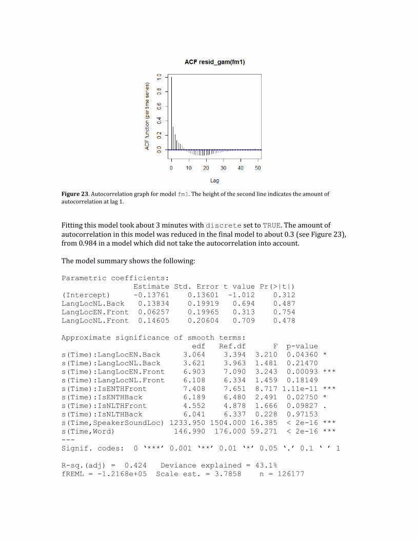
Figure 23. Autocorrelation graph for model fm1. The height of the second line indicates the amount of autocorrelation at lag 1.
Fitting this model took about 3 minutes with discrete set to TRUE. The amount of autocorrelation in this model was reduced in the final model to about 0.3 (see Figure 23), from 0.984 in a model which did not take the autocorrelation into account. The model summary shows the following: Parametric coefficients:
Estimate Std. Error t value Pr(>|t|)
(Intercept) -0.13761 0.13601 -1.012 0.312
LangLocNL.Back 0.13834 0.19919 0.694 0.487
LangLocEN.Front 0.06257 0.19965 0.313 0.754
LangLocNL.Front 0.14605 0.20604 0.709 0.478
Approximate significance of smooth terms:
edf Ref.df F p-value
s(Time):LangLocEN.Back 3.064 3.394 3.210 0.04360 *
s(Time):LangLocNL.Back 3.621 3.963 1.481 0.21470
s(Time):LangLocEN.Front 6.903 7.090 3.243 0.00093 ***
s(Time):LangLocNL.Front 6.108 6.334 1.459 0.18149
s(Time):IsENTHFront 7.408 7.651 8.717 1.11e-11 ***
s(Time):IsENTHBack 6.189 6.480 2.491 0.02750 *
s(Time):IsNLTHFront 4.552 4.878 1.666 0.09827 .
s(Time):IsNLTHBack 6.041 6.337 0.228 0.97153
s(Time,SpeakerSoundLoc) 1233.950 1504.000 16.385 < 2e-16 ***
s(Time,Word) 146.990 176.000 59.271 < 2e-16 ***
---
Signif. codes: 0 ‘***’ 0.001 ‘**’ 0.01 ‘*’ 0.05 ‘.’ 0.1 ‘ ’ 1
R-sq.(adj) = 0.424 Deviance explained = 43.1%
fREML = -1.2168e+05 Scale est. = 3.7858 n = 126177
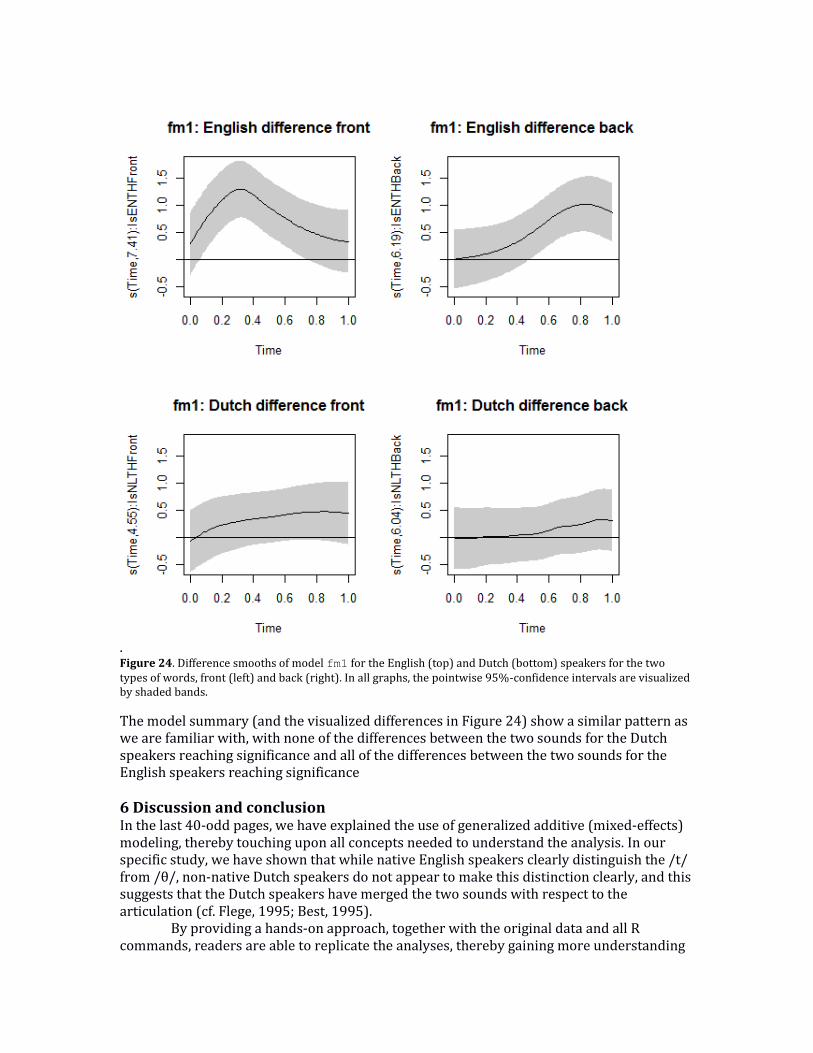
. Figure 24. Difference smooths of model fm1 for the English (top) and Dutch (bottom) speakers for the two types of words, front (left) and back (right). In all graphs, the pointwise 95%-confidence intervals are visualized by shaded bands.
The model summary (and the visualized differences in Figure 24) show a similar pattern as we are familiar with, with none of the differences between the two sounds for the Dutch speakers reaching significance and all of the differences between the two sounds for the English speakers reaching significance 6 Discussion and conclusion In the last 40-odd pages, we have explained the use of generalized additive (mixed-effects) modeling, thereby touching upon all concepts needed to understand the analysis. In our specific study, we have shown that while native English speakers clearly distinguish the /t/ from /θ/, non-native Dutch speakers do not appear to make this distinction clearly, and this suggests that the Dutch speakers have merged the two sounds with respect to the articulation (cf. Flege, 1995; Best, 1995).
By providing a hands-on approach, together with the original data and all R commands, readers are able to replicate the analyses, thereby gaining more understanding
about the material at hand. Importantly, other studies employing generalized additive modeling by Wieling and others have also made their data and code available (e.g., Wieling et al., 2011, 2014, 2016; Meulman et al., 2015, etc.). Thereby making it easy for other researchers to become familiar with the analyses and reproduce the results of these studies. References Akaike, H. (1974). A new look at the statistical model identification. IEEE transactions on
automatic control, 19(6), 716-723. Baayen, R. H. (2008). Analyzing Linguistic Data: A Practical Introduction to Statistics Using R.
Cambridge: Cambridge University Press. Baayen, R. H., Davidson, D. J., & Bates, D. M. (2008). Mixed-effects modeling with crossed
random effects for subjects and items. Journal of memory and language, 59(4), 390-412.
Baayen, H., Vasishth, S., Kliegl, R., & Bates, D. (2017). The cave of shadows: Addressing the human factor with generalized additive mixed models. Journal of Memory and Language, 94, 206-234.
Barr, D.J., Levy, R., Scheepers, C., & Tilly, H. J. (2013). Random effects structure for confirmatory hypothesis testing: Keep it maximal. Journal of Memory and Language, 68, 255–278.
Bates, D., Maechler, M., Bolker, B. M., & Walker, S. (2014). lme4: Linear mixed-effects models using Eigen and S4. R package version 1.1-7.
Best, C. T. (1995). A direct realist perspective on cross-language speech perception. In: W. Strange (Ed.), Speech perception and linguistic experience: Issues in cross-language research. Timonium, MD: York Press, pp. 171-204.
Cederbaum, J., Pouplier, M., Hoole, P., & Greven, S. (2016). Functional linear mixed models for irregularly or sparsely sampled data. Statistical Modelling, 16(1), 67-88.
Efron, B., & Morris, C. N. (1977). Stein's paradox in statistics. WH Freeman. Flege, J. (1995). Second-language speech learning: Theory, findings, and problems. In:
Strange, W. (ed), Speech Perception and Linguistic Experience: Issues in Cross-Language Research, Timonium, MD: York Press, pp. 233-277.
Gubian, M., Torreira, F., & Boves, L. (2015). Using Functional Data Analysis for investigating multidimensional dynamic phonetic contrasts. Journal of Phonetics, 49, 16-40.
Hanulíková, A., & Weber, A. (2012). Sink positive: Linguistic experience with th substitutions influences nonnative word recognition. Attention, Perception, & Psychophysics, 74(3), 613-629.
Hastie, T., & Tibshirani, R. (1986). Generalized additive models. Statistical science, 1, 297-310.
Hay, J., Podlubny, R., Drager, K., & McAuliffe, M. (2017). Car-talk: Location-specific speech production and perception. Journal of Phonetics, 65, 94-109.
Hualde, J. I., Luchkina, T., & Eager, C. D. (2017). Canadian Raising in Chicagoland: The production and perception of a marginal contrast. Journal of Phonetics, 65, 15-44.
Matuschek, H., Kliegl, R., Vasishth, S., Baayen, H., & Bates, D. (2017). Balancing Type I error and power in linear mixed models. Journal of Memory and Language, 94, 305-315.
Meulman, N., Wieling, M., Sprenger, S. A., Stowe, L. A., & Schmid, M. S. (2015). Age effects in L2 grammar processing as revealed by ERPs and how (not) to study them. PloS one, 10(12), e0143328.
Nixon, J. S., van Rij, J., Mok, P., Baayen, R. H., & Chen, Y. (2016). The temporal dynamics of perceptual uncertainty: eye movement evidence from Cantonese segment and tone perception. Journal of Memory and Language, 90, 103-125.
Ots, N. (2017). On the phrase-level function of f0 in Estonian. Journal of Phonetics, 65, 77-93.

Pastätter, M., & Pouplier, M. (2017). Articulatory mechanisms underlying onset-vowel organization. Journal of Phonetics, 65, 1-14.
Sóskuthy, M. (submitted). Generalised additive mixed models for dynamic analysis in linguistics: a practical introduction. arXiv preprint arXiv:1703.05339.
Stuart-Smith, J., Lennon, R., Macdonald, R., Robertson, D., Sóskuthy, M., José, B., & Evers, L. (2015). A dynamic acoustic view of real-time change in word-final liquids in spontaneous glaswegian. Proceedings of the 18th International Congress of Phonetic Sciences, 10-14 August 2015, Glasgow
Tiede, M. (2005). MVIEW: software for visualization and analysis of concurrently recorded movement data. New Haven, CT: Haskins Laboratories.
Van der Harst, S., Van de Velde, H., & Van Hout, R. (2014). Variation in Standard Dutch vowels: The impact of formant measurement methods on identifying the speaker's regional origin. Language Variation and Change, 26(2), 247-272.
van Rij, J., Wieling, M., Baayen, R., and van Rijn, H. (2016). “itsadug: Interpreting Time Series and Autocorrelated Data Using GAMMs.” R package version 2.2.
Yang, J., & Fox, R. A. (2017). L1–L2 interactions of vowel systems in young bilingual Mandarin-English children. Journal of Phonetics, 65, 60-76.
Wieling, M., Nerbonne, J., & Baayen, R. H. (2011). Quantitative social dialectology: Explaining linguistic variation geographically and socially. PLOS ONE, 6(9), e23613.
Wieling, M., Montemagni, S., Nerbonne, J., & Baayen, R. H. (2014). Lexical differences between Tuscan dialects and standard Italian: Accounting for geographic and socio-demographic variation using generalized additive mixed modeling. Language, 90(3), 669-692.
Wieling, M., Tomaschek, F., Arnold, D., Tiede, M., Bröker, F., Thiele, S., ... & Baayen, R. H. (2016). Investigating dialectal differences using articulography. Journal of Phonetics, 59, 122-143.
Winter, B. (2013). Linear models and linear mixed effects models in R with linguistic applications. arXiv:1308.5499.
Winter, B., & Wieling, M. (2016). How to analyze linguistic change using mixed models, Growth Curve Analysis and Generalized Additive Modeling. Journal of Language Evolution, 1(1), 7-18.
Wood, S. (2003). Thin plate regression splines. Journal of the Royal Statistical Society: Series B (Statistical Methodology), 65(1), 95–114.
Wood, S. N. (2011). Fast stable restricted maximum likelihood and marginal likelihood estimation of semiparametric generalized linear models. Journal of the Royal Statistical Society: Series B (Statistical Methodology), 73(1), 3-36.
Wood, S. (2017). Generalized additive models: an introduction with R. 2nd edition. Boca Raton: CRC press.