Generalized Linear Models and Generalized Additive Modelsryantibs/advmethods/shalizi/ch13.pdf · · 2014-05-02Generalized Linear Models and Generalized Additive Models ... The usual

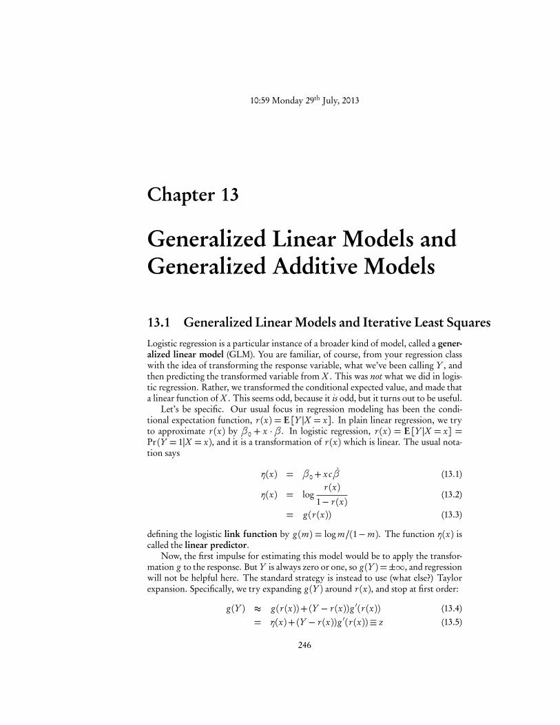
10:59 Monday 29th July, 2013

Chapter 13

Generalized Linear Models andGeneralized Additive Models

13.1 Generalized Linear Models and Iterative Least SquaresLogistic regression is a particular instance of a broader kind of model, called a gener-alized linear model (GLM). You are familiar, of course, from your regression classwith the idea of transforming the response variable, what we’ve been calling Y , andthen predicting the transformed variable from X . This was not what we did in logis-tic regression. Rather, we transformed the conditional expected value, and made thata linear function of X . This seems odd, because it is odd, but it turns out to be useful.

Let’s be specific. Our usual focus in regression modeling has been the condi-tional expectation function, r (x) = E[Y |X = x]. In plain linear regression, we tryto approximate r (x) by �0 + x ·�. In logistic regression, r (x) = E[Y |X = x] =Pr (Y = 1|X = x), and it is a transformation of r (x) which is linear. The usual nota-tion says

⌘(x) = �0+ xc�̇ (13.1)

⌘(x) = logr (x)

1� r (x)(13.2)

= g (r (x)) (13.3)

defining the logistic link function by g (m) = log m/(1�m). The function ⌘(x) iscalled the linear predictor.

Now, the first impulse for estimating this model would be to apply the transfor-mation g to the response. But Y is always zero or one, so g (Y ) =±1, and regressionwill not be helpful here. The standard strategy is instead to use (what else?) Taylorexpansion. Specifically, we try expanding g (Y ) around r (x), and stop at first order:

g (Y ) ⇡ g (r (x))+ (Y � r (x))g 0(r (x)) (13.4)= ⌘(x)+ (Y � r (x))g 0(r (x))⌘ z (13.5)

246

24713.1. GENERALIZED LINEAR MODELS AND ITERATIVE LEAST

SQUARES

We define this to be our effective response after transformation. Notice that if therewere no noise, so that y was always equal to its conditional mean r (x), then regressingz on x would give us back the coefficients �0,�. What this suggests is that we canestimate those parameters by regressing z on x.

The term Y � r (x) has expectation zero, so it acts like the noise, with the factorof g 0 telling us about how the noise is scaled by the transformation. This lets us workout the variance of z:

Var[Z |X = x] = Var[⌘(x)|X = x]+Var⇥(Y � r (x))g 0(r (x))|X = x

⇤(13.6)

= 0+ (g 0(r (x)))2Var[Y |X = x] (13.7)

For logistic regression, with Y binary, Var[Y |X = x] = r (x)(1 � r (x)). On theother hand, with the logistic link function, g 0(r (x)) = 1

r (x)(1�r (x)) . Thus, for logisticregression, Var[Z |X = x] = [r (x)(1� r (x))]�1.

Because the variance of Z changes with X , this is a heteroskedastic regressionproblem. As we saw in chapter 7, the appropriate way of dealing with such a problemis to use weighted least squares, with weights inversely proportional to the variances.This means that the weight at x should be proportional to r (x)(1� r (x)). Noticetwo things about this. First, the weights depend on the current guess about the pa-rameters. Second, we give little weight to cases where r (x) ⇡ 0 or where r (x) ⇡ 1,and the most weight when r (x) = 0.5. This focuses our attention on places where wehave a lot of potential information — the distinction between a probability of 0.499and 0.501 is just a lot easier to discern than that between 0.000 and 0.002!

We can now put all this together into an estimation strategy for logistic regres-sion.

1. Get the data (x1, y1), . . . (xn , yn), and some initial guesses �0,�.

2. until �0,� converge

(a) Calculate ⌘(xi ) =�0+ xi ·� and the corresponding r (xi )

(b) Find the effective transformed responses zi = ⌘(xi )+yi�r (xi )

r (xi )(1�r (xi ))

(c) Calculate the weights wi = r (xi )(1� r (xi ))

(d) Do a weighted linear regression of zi on xi with weights wi , and set�0,�to the intercept and slopes of this regression

Our initial guess about the parameters tells us about the heteroskedasticity, whichwe use to improve our guess about the parameters, which we use to improve our guessabout the variance, and so on, until the parameters stabilize. This is called iterativereweighted least squares (or “iterative weighted least squares”, “iteratively weightedleast squares”, “iteratived reweighted least squares”, etc.), abbreviated IRLS, IRWLS,IWLS, etc. As mentioned in the last chapter, this turns out to be almost equivalent toNewton’s method, at least for this problem.


13.1. GENERALIZED LINEAR MODELS AND ITERATIVE LEASTSQUARES 248

13.1.1 GLMs in General

The set-up for an arbitrary GLM is a generalization of that for logistic regression. Weneed

• A linear predictor, ⌘(x) =�0+ xc�̇

• A link function g , so that ⌘(x) = g (r (x)). For logistic regression, we hadg (r ) = log r/(1� r ).

• A dispersion scale function V , so that Var[Y |X = x] = �2V (r (x)). For lo-gistic regression, we had V (r ) = r (1� r ), and �2 = 1.

With these, we know the conditional mean and conditional variance of the responsefor each value of the input variables x.

As for estimation, basically everything in the IRWLS set up carries over un-changed. In fact, we can go through this algorithm:

1. Get the data (x1, y1), . . . (xn , yn), fix link function g (r ) and dispersion scale func-tion V (r ), and make some initial guesses �0,�.

2. Until �0,� converge

(a) Calculate ⌘(xi ) =�0+ xi ·� and the corresponding r (xi )

(b) Find the effective transformed responses zi = ⌘(xi )+(yi� r (xi ))g 0(r (xi ))

(c) Calculate the weights wi = [(g 0(r (xi ))2V (r (xi ))]�1

(d) Do a weighted linear regression of zi on xi with weights wi , and set�0,�to the intercept and slopes of this regression

Notice that even if we don’t know the over-all variance scale �2, that’s OK, becausethe weights just have to be proportional to the inverse variance.

13.1.2 Examples of GLMs

13.1.2.1 Vanilla Linear Models

To re-assure ourselves that we are not doing anything crazy, let’s see what happenswhen g (r ) = r (the “identity link”), and Var[Y |X = x] = �2, so that V (r ) = 1.Then g 0 = 1, all weights wi = 1, and the effective transformed response zi = yi . Sowe just end up regressing yi on xi with no weighting at all — we do ordinary leastsquares. Since neither the weights nor the transformed response will change, IRWLSwill converge exactly after one step. So if we get rid of all this nonlinearity andheteroskedasticity and go all the way back to our very first days of doing regression,we get the OLS answers we know and love.


24913.1. GENERALIZED LINEAR MODELS AND ITERATIVE LEAST

SQUARES

13.1.2.2 Binomial Regression

In many situations, our response variable yi will be an integer count running between0 and some pre-determined upper limit ni . (Think: number of patients in a hospitalward with some condition, number of children in a classroom passing a test, numberof widgets produced by a factory which are defective, number of people in a villagewith some genetic mutation.) One way to model this would be as a binomial randomvariable, with ni trials, and a success probability pi which was a logistic functionof predictors x. The logistic regression we have done so far is the special case whereni = 1 always. I will leave it as an EXERCISE (1) for you to work out the link functionand the weights for general binomial regression, where the ni are treated as known.

One implication of this model is that each of the ni “trials” aggregated togetherin yi is independent of all the others, at least once we condition on the predictorsx. (So, e.g., whether any student passes the test is independent of whether any oftheir classmates pass, once we have conditioned on, say, teacher quality and averageprevious knowledge.) This may or may not be a reasonable assumption. When thesuccesses or failures are dependent, even after conditioning on the predictors, thebinomial model will be mis-specified. We can either try to get more information,and hope that conditioning on a richer set of predictors makes the dependence goaway, or we can just try to account for the dependence by modifying the variance(“overdispersion” or “underdispersion”); we’ll return to both topics later.

13.1.2.3 Poisson Regression

Recall that the Poisson distribution has probability mass function

p(y) =e�µµy

y!(13.8)

with E[Y ] = Var[Y ] = µ. As you remember from basic probability, a Poissondistribution is what we get from a binomial if the probability of success per trialshrinks towards zero but the number of trials grows to infinity, so that we keep themean number of successes the same:

Binom(n,µ/n)† Pois(µ) (13.9)

This makes the Poisson distribution suitable for modeling counts with no fixed upperlimit, but where the probability that any one of the many individual trials is a successis fairly low. If µ is allowed to be depend on the predictor variables, we get Poissonregression. Since the variance is equal to the mean, Poisson regression is always goingto be heteroskedastic.

Since µ has to be non-negative, a natural link function is g (µ) = logµ. Thisproduces g 0(µ) = 1/µ, and so weights w = µ. When the expected count is large,so is the variance, which normally would reduce the weight put on an observationin regression, but in this case large expected counts also provide more informationabout the coefficients, so they end up getting increasing weight.


13.2. GENERALIZED ADDITIVE MODELS 250

13.1.3 UncertaintyStandard errors for coefficients can be worked out as in the case of weighted leastsquares for linear regression. Confidence intervals for the coefficients will be approx-imately Gaussian in large samples, for the usual likelihood-theory reasons, when themodel is properly specified. One can, of course, also use either a parametric boot-strap, or resampling of cases/data-points to assess uncertainty.

Resampling of residuals can be trickier, because it is not so clear what counts asa residual. When the response variable is continuous, we can get “standardized” or

“Pearson” residuals, ✏̂i =yi�bµ(xi )q€V (µ(xi ))

, resample them to get ✏̃i , and then add ✏̃i

q€V (µ(xi ))

to the fitted values. This does not really work when the response is discrete-valued,however.

13.2 Generalized Additive ModelsIn the development of generalized linear models, we use the link function g to relatethe conditional mean µ(x) to the linear predictor ⌘(x). But really nothing in whatwe were doing required ⌘ to be linear in x. In particular, it all works perfectly wellif ⌘ is an additive function of x. We form the effective responses zi as before, andthe weights wi , but now instead of doing a linear regression on xi we do an additiveregression, using backfitting (or whatever). This gives us a generalized additive model(GAM).

Essentially everything we know about the relationship between linear modelsand additive models carries over. GAMs converge somewhat more slowly as n growsthan do GLMs, but the former have less bias, and strictly include GLMs as specialcases. The transformed (mean) response is related to the predictor variables not justthrough coefficients, but through whole partial response functions. If we want totest whether a GLM is well-specified, we can do so by comparing it to a GAM, andso forth.

In fact, one could even make ⌘(x) an arbitrary smooth function of x, to be es-timated through (say) kernel smoothing of zi on xi . This is rarely done, however,partly because of curse-of-dimensionality issues, but also because, if one is going togo that far, one might as well just use kernels to estimate conditional distributions, aswe will see in Chapter 15.


251 13.3. WEATHER FORECASTING IN SNOQUALMIE FALLS

13.3 Weather Forecasting in Snoqualmie FallsTo make the use of logistic regression and GLMs concrete, we are going to build asimple weather forecaster. Our data consist of daily records, from the beginning of1948 to the end of 1983, of precipitation at Snoqualmie Falls, Washington (Figure13.1)1. Each row of the data file is a different year; each column records, for that dayof the year, the day’s precipitation (rain or snow), in units of 1

100 inch. Because ofleap-days, there are 366 columns, with the last column having an NA value for threeout of four years.

snoqualmie <- read.csv("snoqualmie.csv",header=FALSE)# Turn into one big vector without year breakssnoqualmie <- unlist(snoqualmie)# Remove NAs from non-leap-yearssnoqualmie <- na.omit(snoqualmie)

What we want to do is predict tomorrow’s weather from today’s. This wouldbe of interest if we lived in Snoqualmie Falls, or if we operated either one of thelocal hydroelectric power plants, or the tourist attraction of the Falls themselves.Examining the distribution of the data (Figures 13.2 and 13.3) shows that there is abig spike in the distribution at zero precipitation, and that days of no precipitationcan follow days of any amount of precipitation but seem to be less common afterheavy precipitation.

These facts suggest that “no precipitation” is a special sort of event which wouldbe worth predicting in its own right (as opposed to just being when the precipitationhappens to be zero), so we will attempt to do so with logistic regression. Specifically,the input variable Xi will be the amount of precipitation on the i th day, and theresponse Yi will be the indicator variable for whether there was any precipitation onday i + 1 — that is, Yi = 1 if Xi+1 > 0, an Yi = 0 if Xi+1 = 0. We expect from Figure13.3, as well as common experience, that the coefficient on X should be positive.2

Before fitting the logistic regression, it’s convenient to re-shape the data:

vector.to.pairs <- function(v) {v <- as.numeric(v)n <- length(v)return(cbind(v[-1],v[-n]))

}snoq.pairs <- vector.to.pairs(snoqualmie)colnames(snoq.pairs) <- c("tomorrow","today")snoq <- as.data.frame(snoq.pairs)

This creates a two-column array, where the first column is the precipitation on dayi+1, and the second column is the precipitation on day i (hence the column names).Finally, I turn the whole thing into a data frame.

1I learned of this data set from Guttorp (1995); the data file is available from http://www.stat.washington.edu/peter/stoch.mod.data.html.

2This does not attempt to model how much precipitation there will be tomorrow, if there is any. Wecould make that a separate model, if we can get this part right.


13.3. WEATHER FORECASTING IN SNOQUALMIE FALLS 252

Figure 13.1: Snoqualmie Falls, Washington, on a sunny day. Photo byJeannine Hall Gailey, from http://myblog.webbish6.com/2011/07/17-years-and-hoping-for-another-17.html. [[TODO: Get permissionfor photo use!]]



Histogram of snoqualmie

Precipitation (1/100 inch)

Density

0 100 200 300 400

0.00

0.02

0.04

0.06

plot(hist(snoqualmie,n=50,probability=TRUE),xlab="Precipitation (1/100 inch)")rug(snoqualmie,col="grey")

Figure 13.2: Histogram of the amount of daily precipitation at Snoqualmie Falls



0 100 200 300 400

0100

200

300

400

Precipitation today (1/100 inch)

Pre

cipi

tatio

n to

mor

row

(1/1

00 in

ch)

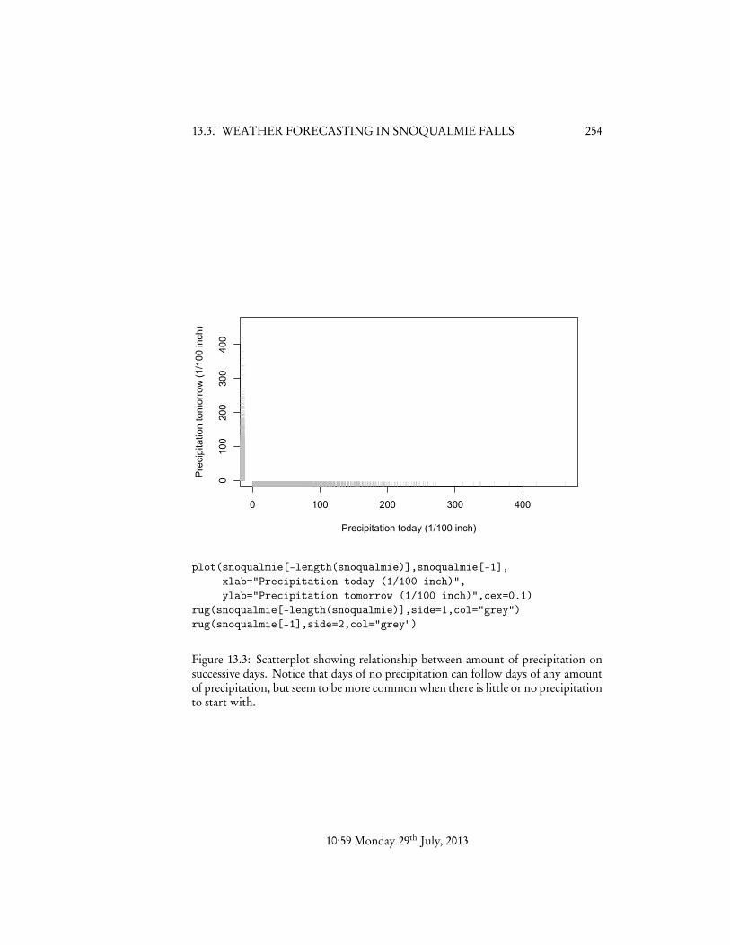
plot(snoqualmie[-length(snoqualmie)],snoqualmie[-1],xlab="Precipitation today (1/100 inch)",ylab="Precipitation tomorrow (1/100 inch)",cex=0.1)

rug(snoqualmie[-length(snoqualmie)],side=1,col="grey")rug(snoqualmie[-1],side=2,col="grey")

Figure 13.3: Scatterplot showing relationship between amount of precipitation onsuccessive days. Notice that days of no precipitation can follow days of any amountof precipitation, but seem to be more common when there is little or no precipitationto start with.



Now fitting is straightforward:

snoq.logistic <- glm((tomorrow > 0) ~ today, data=snoq, family=binomial)

To see what came from the fitting, run summary:

> summary(snoq.logistic)

Call:glm(formula = (tomorrow > 0) ~ today, family = binomial, data = snoq)

Deviance Residuals:Min 1Q Median 3Q Max

-2.3713 -1.1805 0.9536 1.1693 1.1744

Coefficients:Estimate Std. Error z value Pr(>|z|)

(Intercept) 0.0071899 0.0198430 0.362 0.717today 0.0059232 0.0005858 10.111 <2e-16 ***---

(I have cut off some uninformative bits of the output.) The coefficient on X , theamount of precipitation today, is indeed positive, and (if we can trust R’s calcula-tions) highly significant. There is also an intercept term, which is slight positive,but not very significant. We can see what the intercept term means by consideringwhat happens when X = 0, i.e., on days of no precipitation. The linear predictor isthen 0.0072+ 0 ⇤ (0.0059) = 0.0072, and the predicted probability of precipitation ise0.0072/(1+ e0.0072) = 0.502. That is, even when there is no precipitation today, wepredict that it is slightly more probable than not that there will be some precipitationtomorrow.3

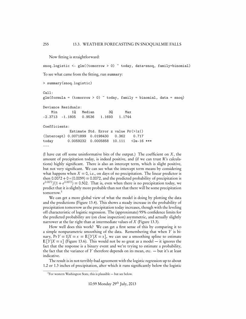
We can get a more global view of what the model is doing by plotting the dataand the predictions (Figure 13.4). This shows a steady increase in the probability ofprecipitation tomorrow as the precipitation today increases, though with the levelingoff characteristic of logistic regression. The (approximate) 95% confidence limits forthe predicted probability are (on close inspection) asymmetric, and actually slightlynarrower at the far right than at intermediate values of X (Figure 13.3).

How well does this work? We can get a first sense of this by comparing it toa simple nonparametric smoothing of the data. Remembering that when Y is bi-nary, PrY = 1|X = x = E[Y |X = x], we can use a smoothing spline to estimateE[Y |X = x] (Figure 13.6). This would not be so great as a model — it ignores thefact that the response is a binary event and we’re trying to estimate a probability,the fact that the variance of Y therefore depends on its mean, etc. — but it’s at leastindicative.

The result is in not-terribly-bad agreement with the logistic regression up to about1.2 or 1.3 inches of precipitation, after which it runs significantly below the logistic

3For western Washington State, this is plausible — but see below.



0 100 200 300 400

0.0

0.2

0.4

0.6

0.8

1.0


Pos

itive

pre

cipi

tatio

n to

mor

row

?

plot((tomorrow>0)~today,data=snoq,xlab="Precipitation today (1/100 inch)",ylab="Positive precipitation tomorrow?")

rug(snoq$today,side=1,col="grey")

data.plot <- data.frame(today=(0:500))logistic.predictions <- predict(snoq.logistic,newdata=data.plot,se.fit=TRUE)lines(0:500,ilogit(logistic.predictions$fit))lines(0:500,ilogit(logistic.predictions$fit+1.96*logistic.predictions$se.fit),

lty=2)lines(0:500,ilogit(logistic.predictions$fit-1.96*logistic.predictions$se.fit),

lty=2)

Figure 13.4: Data (dots), plus predicted probabilities (solid line) and approximate95% confidence intervals from the logistic regression model (dashed lines). Note thatcalculating standard errors for predictions on the logit scale, and then transforming,is better practice than getting standard errors directly on the probability scale.



0 100 200 300 400 500

0.01

0.02

0.03

0.04

Difference in probability between prediction and confidence limit for prediction


Δprobability

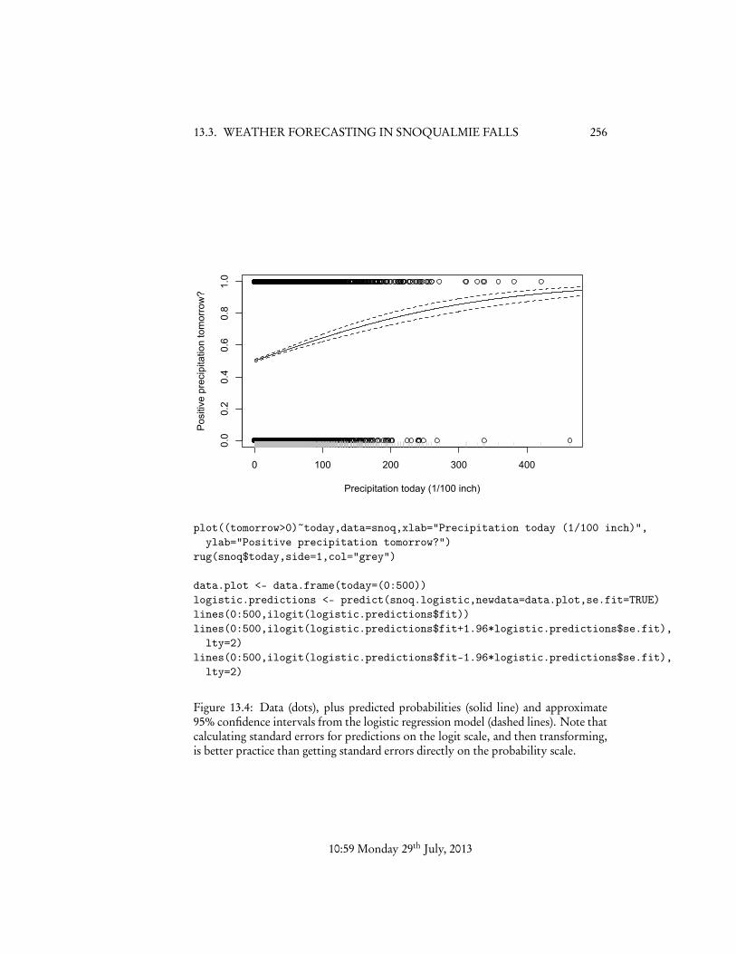
plot(0:500,ilogit(logistic.predictions$fit)-ilogit(logistic.predictions$fit-1.96*logistic.predictions$se.fit),type="l",col="blue",xlab="Precipitation today (1/100 inch)",main="Difference in probability between prediction\n

and confidence limit for prediction",ylab = expression(paste(Delta,"probability")))

lines(0:500,ilogit(logistic.predictions$fit+1.96*logistic.predictions$se.fit)-ilogit(logistic.predictions$fit))

Figure 13.5: Distance from the fitted probability to the upper (black) and lower (blue)confidence limits. Notice that the two are not equal, and somewhat smaller at verylarge values of X than at intermediate ones. (Why?)



0 100 200 300 400

0.0

0.2

0.4

0.6

0.8

1.0


Pos

itive

pre

cipi

tatio

n to

mor

row

?

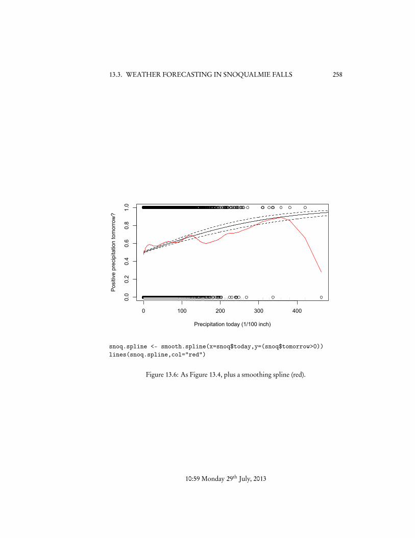
snoq.spline <- smooth.spline(x=snoq$today,y=(snoq$tomorrow>0))lines(snoq.spline,col="red")

Figure 13.6: As Figure 13.4, plus a smoothing spline (red).



regression, rejoins it around 3.5 inches of precipitation, and then (as it were) falls offa cliff.

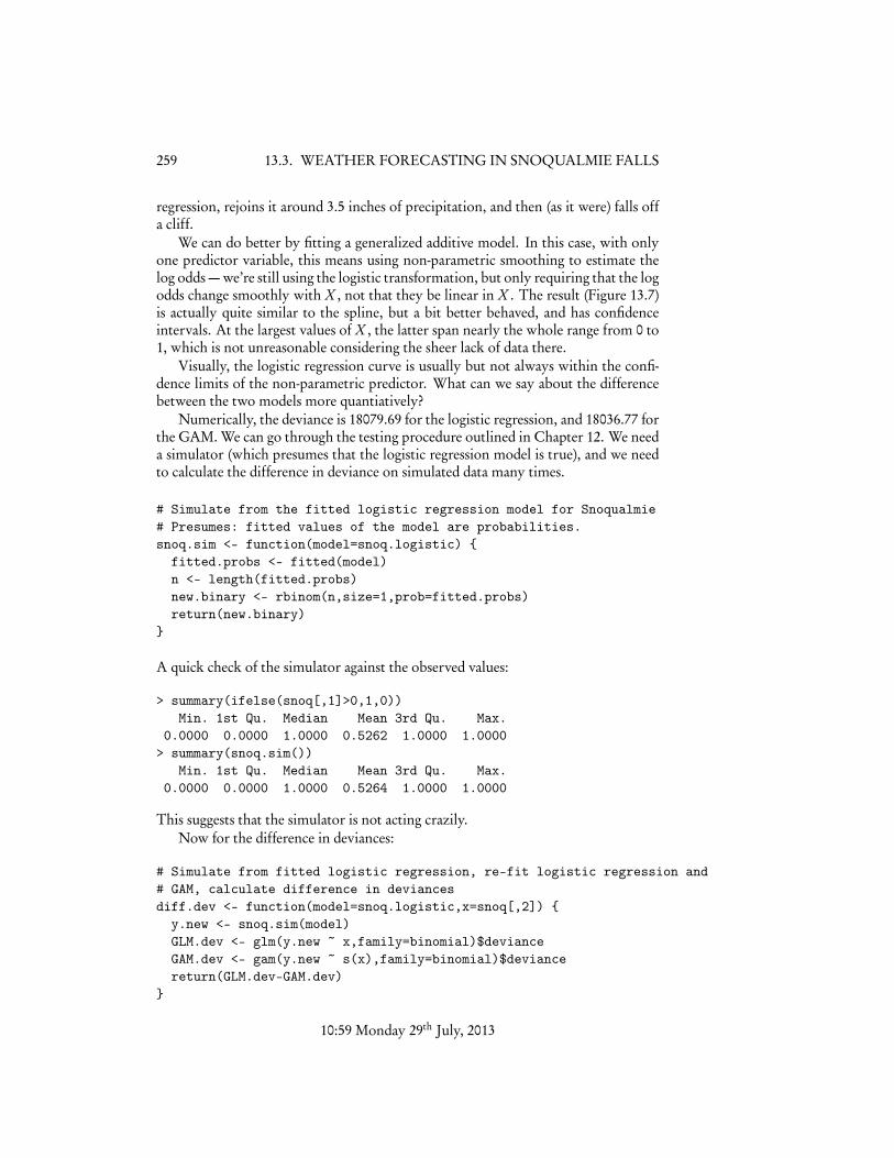
We can do better by fitting a generalized additive model. In this case, with onlyone predictor variable, this means using non-parametric smoothing to estimate thelog odds — we’re still using the logistic transformation, but only requiring that the logodds change smoothly with X , not that they be linear in X . The result (Figure 13.7)is actually quite similar to the spline, but a bit better behaved, and has confidenceintervals. At the largest values of X , the latter span nearly the whole range from 0 to1, which is not unreasonable considering the sheer lack of data there.

Visually, the logistic regression curve is usually but not always within the confi-dence limits of the non-parametric predictor. What can we say about the differencebetween the two models more quantiatively?

Numerically, the deviance is 18079.69 for the logistic regression, and 18036.77 forthe GAM. We can go through the testing procedure outlined in Chapter 12. We needa simulator (which presumes that the logistic regression model is true), and we needto calculate the difference in deviance on simulated data many times.

# Simulate from the fitted logistic regression model for Snoqualmie# Presumes: fitted values of the model are probabilities.snoq.sim <- function(model=snoq.logistic) {

fitted.probs <- fitted(model)n <- length(fitted.probs)new.binary <- rbinom(n,size=1,prob=fitted.probs)return(new.binary)

}

A quick check of the simulator against the observed values:

> summary(ifelse(snoq[,1]>0,1,0))Min. 1st Qu. Median Mean 3rd Qu. Max.

0.0000 0.0000 1.0000 0.5262 1.0000 1.0000> summary(snoq.sim())

Min. 1st Qu. Median Mean 3rd Qu. Max.0.0000 0.0000 1.0000 0.5264 1.0000 1.0000

This suggests that the simulator is not acting crazily.Now for the difference in deviances:

# Simulate from fitted logistic regression, re-fit logistic regression and# GAM, calculate difference in deviancesdiff.dev <- function(model=snoq.logistic,x=snoq[,2]) {

y.new <- snoq.sim(model)GLM.dev <- glm(y.new ~ x,family=binomial)$devianceGAM.dev <- gam(y.new ~ s(x),family=binomial)$deviancereturn(GLM.dev-GAM.dev)

}



0 100 200 300 400

0.0

0.2

0.4

0.6

0.8

1.0


Pos

itive

pre

cipi

tatio

n to

mor

row

?

library(mgcv)snoq.gam <- gam((tomorrow>0)~s(today),data=snoq,family=binomial)gam.predictions <- predict.gam(snoq.gam,newdata=data.plot,se.fit=TRUE)lines(0:500,ilogit(gam.predictions$fit),col="blue")lines(0:500,ilogit(gam.predictions$fit+1.96*gam.predictions$se.fit),

col="blue",lty=2)lines(0:500,ilogit(gam.predictions$fit-1.96*gam.predictions$se.fit),

col="blue",lty=2)

Figure 13.7: As Figure 13.6, but with the addition of a generalized additive model(blue line) and its confidence limits (dashed blue lines). Note: the predict functionin the gam package does not allow one to calculate standard errors for new data. Youmay need to un-load the gam library first, with detach(package:gam).



A single run of this takes about 1.5 seconds on my computer.Finally, we calculate the distribution of difference in deviances under the null

(that the logistic regression is properly specified), and the corresponding p-value:

diff.dev.obs <- snoq.logistic$deviance - snoq.gam$deviancenull.dist.of.diff.dev <- replicate(1000,diff.dev())p.value <- (1+sum(null.dist.of.diff.dev > diff.dev.obs))/(1+length(null.dist.of.diff.dev))

Using a thousand replicates takes about 1500 seconds, or roughly 25 minutes, whichis substantial, but not impossible; it gave a p-value of < 10�3, and the followingsampling distribution:

> summary(null.dist.of.diff.dev)Min. 1st Qu. Median Mean 3rd Qu. Max.

0.000097 0.002890 0.016770 2.267000 2.897000 29.750000

(A preliminary trial run of only 100 replicates, taking a few minutes, gave

> summary(null.dist.of.diff.dev)Min. 1st Qu. Median Mean 3rd Qu. Max.

0.000291 0.002681 0.013700 2.008000 2.121000 27.820000

which implies a p-value of < 0.01. This would be good enough for many practicalpurposes.)

Having detected that there is a problem with the GLM, we can ask where it lies.We could just use the GAM, but it’s more interesting to try to diagnose what’s goingon.

In this respect Figure 13.7 is actually a little misleading, because it leads the eyeto emphasize the disagreement between the models at large X , when actually thereare very few data points there, and so even large differences in predicted probabili-ties there contribute little to the over-all likelihood difference. What is actually moreimportant is what happens at X = 0, which contains a very large number of observa-tions (about 47% of all observations), and which we have reason to think is a specialvalue anyway.

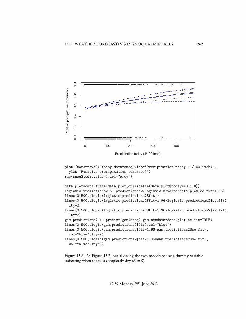
Let’s try introducing a dummy variable for X = 0 into the logistic regression,and see what happens. It will be convenient to augment the data frame with an extracolumn, recording 1 whenever X = 0 and 0 otherwise.

snoq2 <- data.frame(snoq,dry=ifelse(snoq$today==0,1,0))snoq2.logistic <- glm((tomorrow > 0) ~ today + dry,data=snoq2,family=binomial)snoq2.gam <- gam((tomorrow > 0) ~ s(today) + dry,data=snoq2,family=binomial)

Notice that I allow the GAM to treat zero as a special value as well, by giving it accessto that dummy variable. In principle, with enough data it can decide whether or notthat is useful on its own, but since we have guessed that it is, we might as well includeit. Figure 13.8 shows the data and the two new models. These are extremely close toeach other. The new GLM has a deviance of 18015.65, lower than even the GAMbefore, and the new GAM has a deviance of 18015.21. The p-value is essentially



0 100 200 300 400

0.0

0.2

0.4

0.6

0.8

1.0


Pos

itive

pre

cipi

tatio

n to

mor

row

?

plot((tomorrow>0)~today,data=snoq,xlab="Precipitation today (1/100 inch)",ylab="Positive precipitation tomorrow?")

rug(snoq$today,side=1,col="grey")

data.plot=data.frame(data.plot,dry=ifelse(data.plot$today==0,1,0))logistic.predictions2 <- predict(snoq2.logistic,newdata=data.plot,se.fit=TRUE)lines(0:500,ilogit(logistic.predictions2$fit))lines(0:500,ilogit(logistic.predictions2$fit+1.96*logistic.predictions2$se.fit),

lty=2)lines(0:500,ilogit(logistic.predictions2$fit-1.96*logistic.predictions2$se.fit),

lty=2)gam.predictions2 <- predict.gam(snoq2.gam,newdata=data.plot,se.fit=TRUE)lines(0:500,ilogit(gam.predictions2$fit),col="blue")lines(0:500,ilogit(gam.predictions2$fit+1.96*gam.predictions2$se.fit),

col="blue",lty=2)lines(0:500,ilogit(gam.predictions2$fit-1.96*gam.predictions2$se.fit),

col="blue",lty=2)

Figure 13.8: As Figure 13.7, but allowing the two models to use a dummy variableindicating when today is completely dry (X = 0).



1 — and yet we know that this test does have power to detect departures from theparametric model. This is very promising.

Let’s turn now to looking at calibration. The actual fraction of no-precipitationdays which are followed by precipitation is

> mean(snoq$tomorrow[snoq$today==0]>0)[1] 0.4702199

What does the new logistic model predict?

> predict(snoq2.logistic,newdata=data.frame(today=0,dry=1),type="response")1

0.4702199

This should not be surprising — we’ve given the model a special parameter dedi-cated to getting this one probability exactly right! The hope however is that this willchange the predictions made on days with precipitation so that they are better.

Looking at a histogram of fitted values (hist(fitted(snoq2.logistic))) showsa gap in the distribution of predicted probabilities between 0.47 and about 0.55, sowe’ll look first at days where the predicted probability is between 0.55 and 0.56.

> mean(snoq$tomorrow[(fitted(snoq2.logistic) >= 0.55)& (fitted(snoq2.logistic) < 0.56)] > 0)

[1] 0.5474882

Not bad — but a bit painful to write out. Let’s write a function:

frequency.vs.probability <- function(p.lower,p.upper=p.lower+0.01,model=snoq2.logistic,events=(snoq$tomorrow>0)) {fitted.probs <- fitted(model)indices <- (fitted.probs >= p.lower) & (fitted.probs < p.upper)ave.prob <- mean(fitted.probs[indices])frequency <- mean(events[indices])se <- sqrt(ave.prob*(1-ave.prob)/sum(indices))out <- list(frequency=frequency,ave.prob=ave.prob,se=se)return(out)

}

I have added a calculation of the average predicted probability, and a crude estimateof the standard error we should expect if the observations really are binomial withthe predicted probabilities4. Try the function out before doing anything rash:

> frequency.vs.probability(0.55)$frequency[1] 0.5474882

$ave.prob4This could be improved by averaging predicted variances for each point, but using probability ranges

of 0.01 makes it hardly worth the effort.


13.4. EXERCISES 264

[1] 0.5548081

$se[1] 0.00984567

This agrees with our previous calculation.Now we can do this for a lot of probability brackets:

f.vs.p <- sapply((55:74)/100,frequency.vs.probability)

This comes with some unfortunate R cruft, removable thus

f.vs.p <- data.frame(frequency=unlist(f.vs.p["frequency",]),ave.prob=unlist(f.vs.p["ave.prob",]),se=unlist(f.vs.p["se",]))

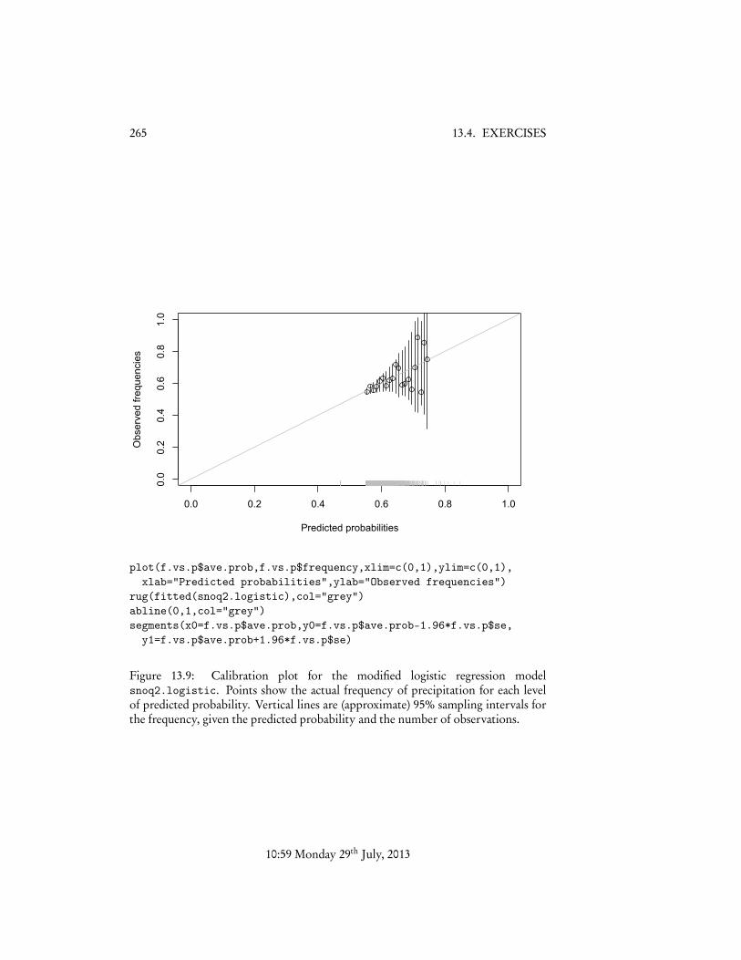
and we’re ready to plot (Figure 13.9). The observed frequencies are generally quitenear to the predicted probabilites, especially when the number of observations islarge and so the sample frequency should be close to the true probability. While Iwouldn’t want to say this was the last word in weather forecasting5, it’s surprisinglygood for such a simple model.

13.4 Exercises1. In binomial regression, we have Y |X = x Binom(n, p(x)), where p(x) follows

a logistic model. Work out the link function g (µ), the variance function V (µ),and the weights w, assuming that n is known and not random.

2. Homework 5, on predicting the death rate in Chicago, is a good candidatefor using Poisson regression. Repeat the exercises in that problem set withPoisson-response GAMs. How do the estimated functions change? Why isthis any different from just taking the log of the death counts, as we did in thehomework?

5There is an extensive discussion of this data in chapter 2 of Guttorp’s book, including many significantrefinements, such as dependence across multiple days.


265 13.4. EXERCISES

0.0 0.2 0.4 0.6 0.8 1.0

0.0

0.2

0.4

0.6

0.8

1.0

Predicted probabilities

Obs

erve

d fre

quen

cies

plot(f.vs.p$ave.prob,f.vs.p$frequency,xlim=c(0,1),ylim=c(0,1),xlab="Predicted probabilities",ylab="Observed frequencies")

rug(fitted(snoq2.logistic),col="grey")abline(0,1,col="grey")segments(x0=f.vs.p$ave.prob,y0=f.vs.p$ave.prob-1.96*f.vs.p$se,

y1=f.vs.p$ave.prob+1.96*f.vs.p$se)

Figure 13.9: Calibration plot for the modified logistic regression modelsnoq2.logistic. Points show the actual frequency of precipitation for each levelof predicted probability. Vertical lines are (approximate) 95% sampling intervals forthe frequency, given the predicted probability and the number of observations.


Documents

Generalized Linear Models and Generalized Additive Modelsryantibs/advmethods/shalizi/ch13.pdf · · 2014-05-02Generalized Linear Models and Generalized Additive Models ... The usual