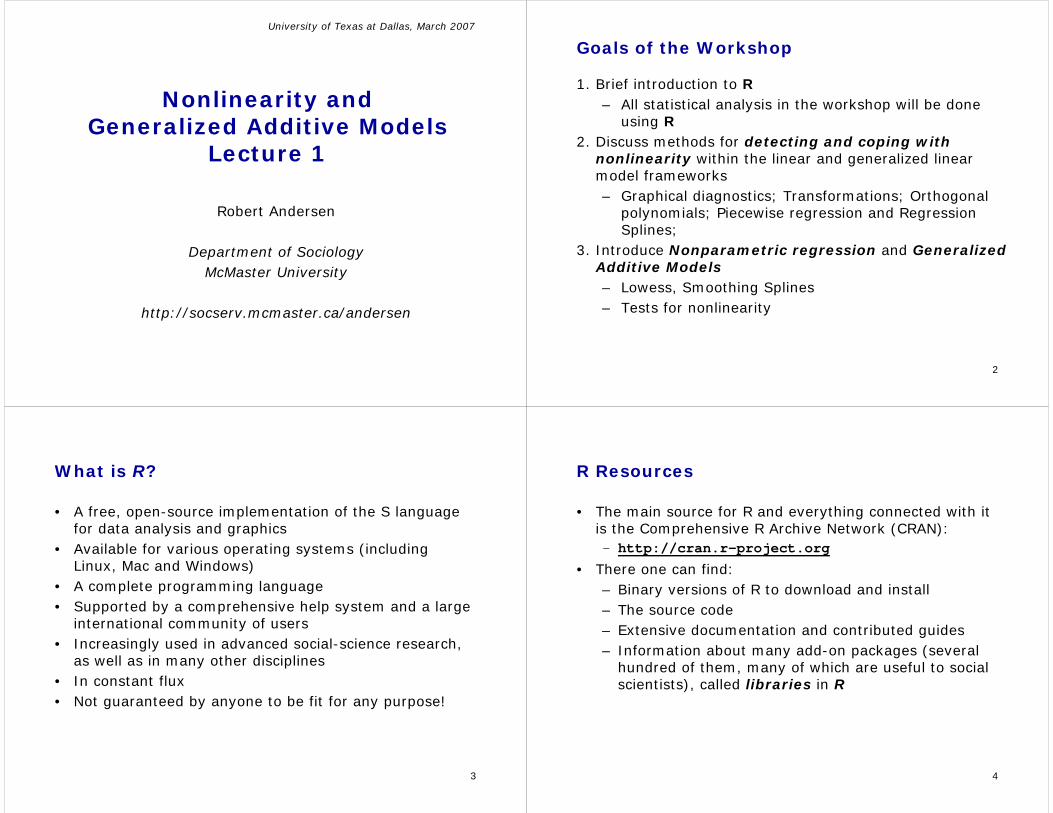
University of Texas at Dallas, March 2007

Nonlinearity and Generalized Additive Models

Lecture 1

Robert Andersen

Department of SociologyMcMaster University

http://socserv.mcmaster.ca/andersen

2

Goals of the Workshop

1. Brief introduction to R– All statistical analysis in the workshop will be done

using R2. Discuss methods for detecting and coping with

nonlinearity within the linear and generalized linear model frameworks– Graphical diagnostics; Transformations; Orthogonal

polynomials; Piecewise regression and Regression Splines;

3. Introduce Nonparametric regression and Generalized Additive Models– Lowess, Smoothing Splines– Tests for nonlinearity

3

What is R?

• A free, open-source implementation of the S language for data analysis and graphics

• Available for various operating systems (including Linux, Mac and Windows)

• A complete programming language• Supported by a comprehensive help system and a large

international community of users• Increasingly used in advanced social-science research,

as well as in many other disciplines• In constant flux• Not guaranteed by anyone to be fit for any purpose!

4

R Resources

• The main source for R and everything connected with it is the Comprehensive R Archive Network (CRAN):– http://cran.r-project.org

• There one can find:– Binary versions of R to download and install– The source code– Extensive documentation and contributed guides– Information about many add-on packages (several

hundred of them, many of which are useful to social scientists), called libraries in R

5

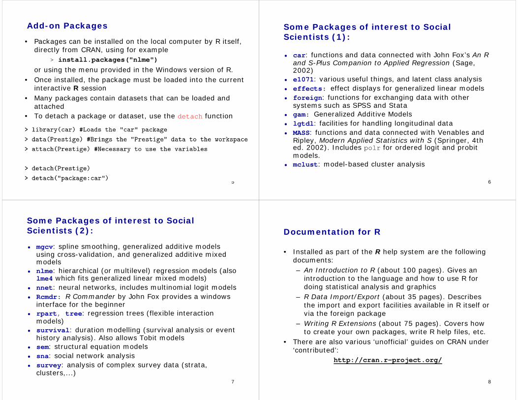
Add-on Packages

• Packages can be installed on the local computer by R itself, directly from CRAN, using for example

> install.packages("nlme")or using the menu provided in the Windows version of R.

• Once installed, the package must be loaded into the current interactive R session

• Many packages contain datasets that can be loaded and attached

• To detach a package or dataset, use the detach function

6

Some Packages of interest to Social Scientists (1):

• car: functions and data connected with John Fox’s An R and S-Plus Companion to Applied Regression (Sage, 2002)

• e1071: various useful things, and latent class analysis• effects: effect displays for generalized linear models • foreign: functions for exchanging data with other

systems such as SPSS and Stata• gam: Generalized Additive Models • lgtdl: facilities for handling longitudinal data• MASS: functions and data connected with Venables and

Ripley, Modern Applied Statistics with S (Springer, 4th ed. 2002). Includes polr for ordered logit and probitmodels.

• mclust: model-based cluster analysis

7

Some Packages of interest to Social Scientists (2):

• mgcv: spline smoothing, generalized additive modelsusing cross-validation, and generalized additive mixed models

• nlme: hierarchical (or multilevel) regression models (also lme4 which fits generalized linear mixed models)

• nnet: neural networks, includes multinomial logit models• Rcmdr: R Commander by John Fox provides a windows

interface for the beginner• rpart, tree: regression trees (flexible interaction

models)• survival: duration modelling (survival analysis or event

history analysis). Also allows Tobit models• sem: structural equation models• sna: social network analysis• survey: analysis of complex survey data (strata,

clusters,...)8

Documentation for R

• Installed as part of the R help system are the following documents:– An Introduction to R (about 100 pages). Gives an

introduction to the language and how to use R for doing statistical analysis and graphics

– R Data Import/Export (about 35 pages). Describes the import and export facilities available in R itself or via the foreign package

– Writing R Extensions (about 75 pages). Covers how to create your own packages, write R help files, etc.

• There are also various ‘unofficial’ guides on CRAN under ‘contributed’:

http://cran.r-project.org/

9

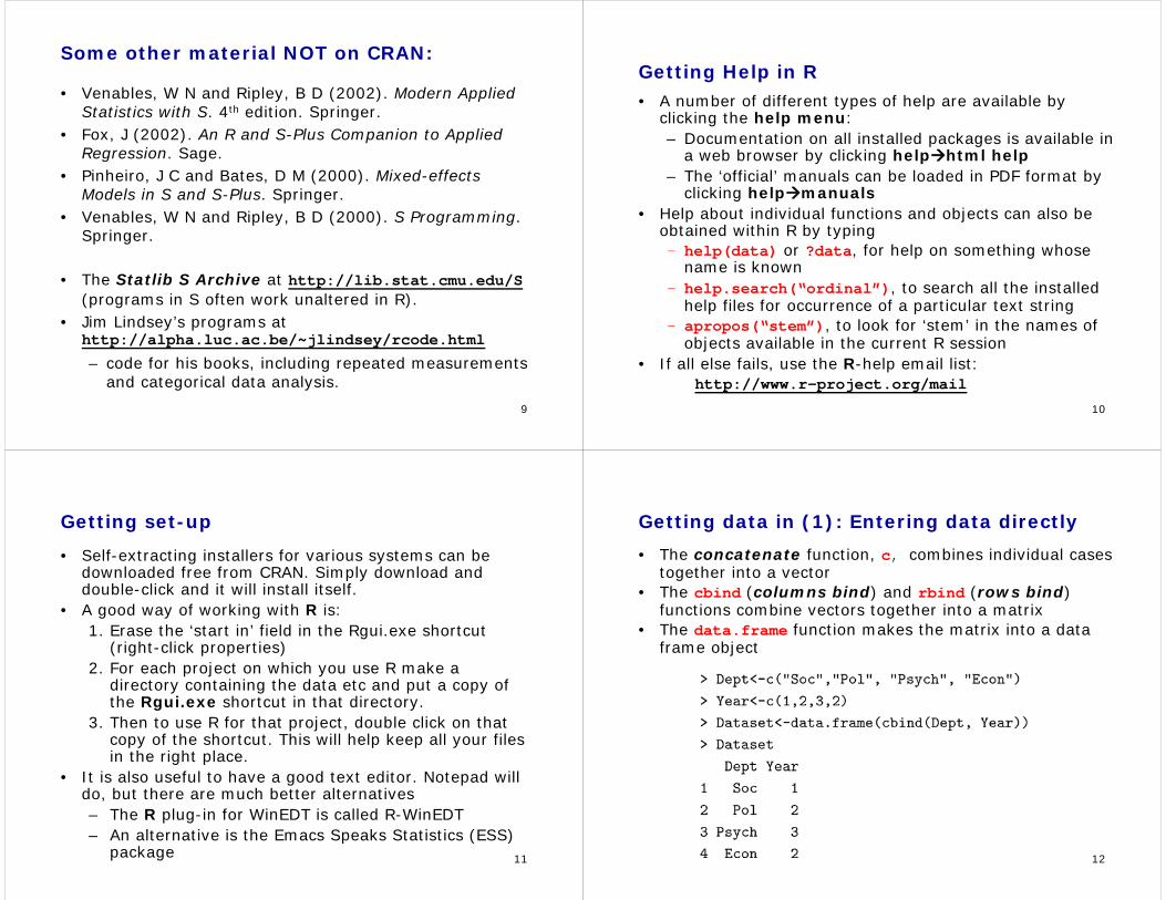
Some other material NOT on CRAN:

• Venables, W N and Ripley, B D (2002). Modern Applied Statistics with S. 4th edition. Springer.

• Fox, J (2002). An R and S-Plus Companion to Applied Regression. Sage.

• Pinheiro, J C and Bates, D M (2000). Mixed-effects Models in S and S-Plus. Springer.

• Venables, W N and Ripley, B D (2000). S Programming. Springer.

• The Statlib S Archive at http://lib.stat.cmu.edu/S(programs in S often work unaltered in R).

• Jim Lindsey’s programs at http://alpha.luc.ac.be/~jlindsey/rcode.html– code for his books, including repeated measurements

and categorical data analysis.

10

Getting Help in R• A number of different types of help are available by

clicking the help menu:– Documentation on all installed packages is available in

a web browser by clicking help html help– The ‘official’ manuals can be loaded in PDF format by

clicking help manuals• Help about individual functions and objects can also be

obtained within R by typing – help(data) or ?data, for help on something whose

name is known– help.search(“ordinal”), to search all the installed

help files for occurrence of a particular text string– apropos(“stem”), to look for ‘stem’ in the names of

objects available in the current R session• If all else fails, use the R-help email list:

http://www.r-project.org/mail

11

Getting set-up

• Self-extracting installers for various systems can be downloaded free from CRAN. Simply download and double-click and it will install itself.

• A good way of working with R is:1. Erase the ‘start in’ field in the Rgui.exe shortcut

(right-click properties)2. For each project on which you use R make a

directory containing the data etc and put a copy of the Rgui.exe shortcut in that directory.

3. Then to use R for that project, double click on that copy of the shortcut. This will help keep all your files in the right place.

• It is also useful to have a good text editor. Notepad will do, but there are much better alternatives– The R plug-in for WinEDT is called R-WinEDT– An alternative is the Emacs Speaks Statistics (ESS)

package 12

Getting data in (1): Entering data directly

• The concatenate function, c, combines individual cases together into a vector

• The cbind (columns bind) and rbind (rows bind) functions combine vectors together into a matrix

• The data.frame function makes the matrix into a data frame object

13

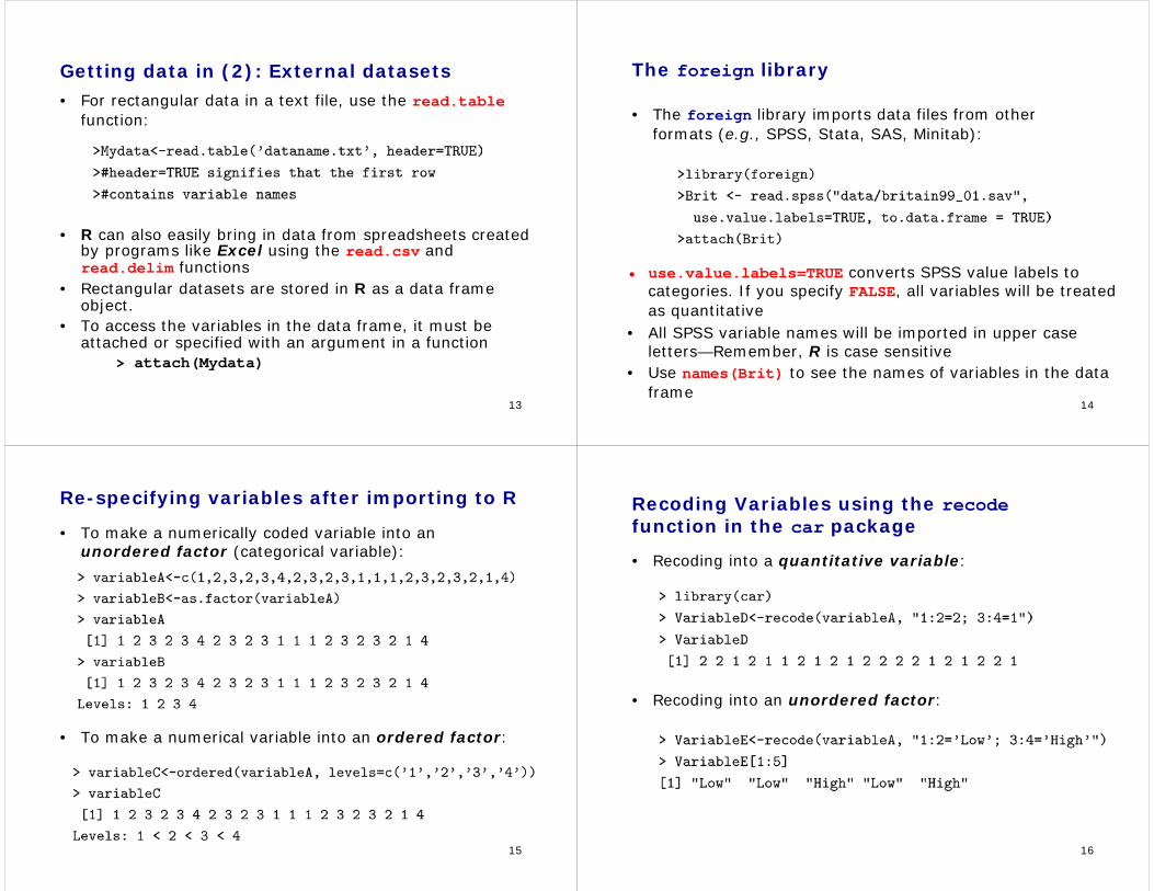
Getting data in (2): External datasets

• For rectangular data in a text file, use the read.tablefunction:

• R can also easily bring in data from spreadsheets created by programs like Excel using the read.csv and read.delim functions

• Rectangular datasets are stored in R as a data frame object.

• To access the variables in the data frame, it must be attached or specified with an argument in a function

> attach(Mydata)

14

The foreign library

• The foreign library imports data files from other formats (e.g., SPSS, Stata, SAS, Minitab):

• use.value.labels=TRUE converts SPSS value labels to categories. If you specify FALSE, all variables will be treated as quantitative

• All SPSS variable names will be imported in upper case letters—Remember, R is case sensitive

• Use names(Brit) to see the names of variables in the data frame

15

Re-specifying variables after importing to R

• To make a numerically coded variable into an unordered factor (categorical variable):

• To make a numerical variable into an ordered factor:

16

Recoding Variables using the recodefunction in the car package

• Recoding into a quantitative variable:

• Recoding into an unordered factor:

17

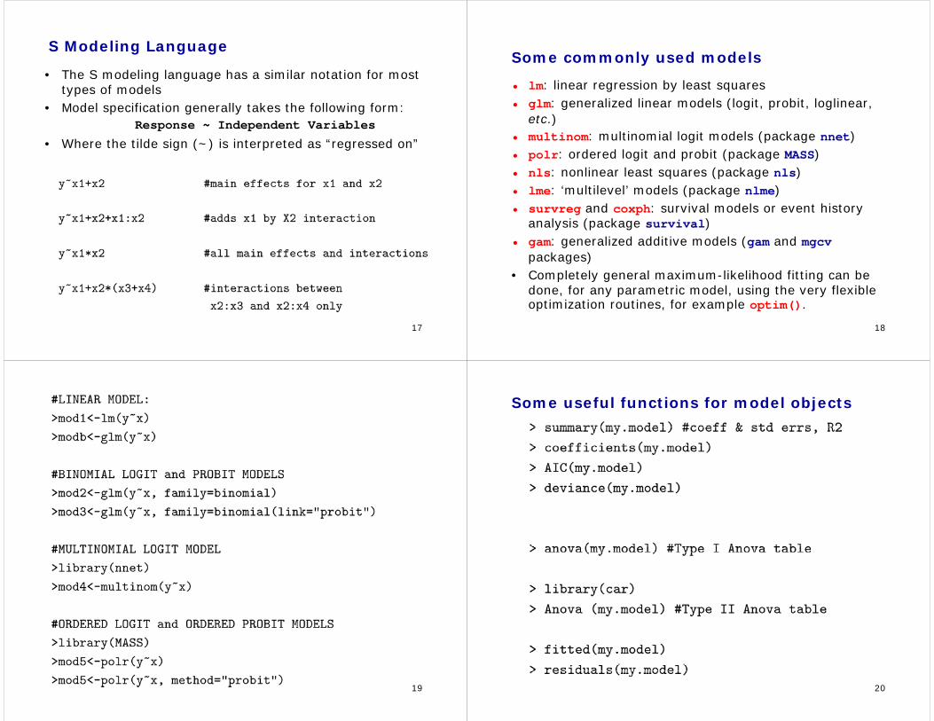
S Modeling Language

• The S modeling language has a similar notation for most types of models

• Model specification generally takes the following form:Response ~ Independent Variables

• Where the tilde sign (~) is interpreted as “regressed on”

18

Some commonly used models

• lm: linear regression by least squares• glm: generalized linear models (logit, probit, loglinear,

etc.)• multinom: multinomial logit models (package nnet)• polr: ordered logit and probit (package MASS)• nls: nonlinear least squares (package nls)• lme: ‘multilevel’ models (package nlme)• survreg and coxph: survival models or event history

analysis (package survival)• gam: generalized additive models (gam and mgcv

packages) • Completely general maximum-likelihood fitting can be

done, for any parametric model, using the very flexible optimization routines, for example optim().

19 20

Some useful functions for model objects

21

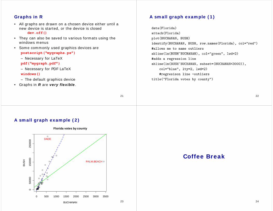
Graphs in R

• All graphs are drawn on a chosen device either until a new device is started, or the device is closed

dev.off()• They can also be saved to various formats using the

windows menus• Some commonly used graphics devices are

postscript(“mygraphs.ps”)– Necessary for LaTeXpdf(“mygraph.pdf”)– Necessary for PDF LaTeXwindows()– The default graphics device

• Graphs in R are very flexible.

22

A small graph example (1)

23

A small graph example (2)

0 500 1000 1500 2000 2500 3000 3500

050

000

1500

0025

0000

BUCHANAN

BUSH

DADE

PALM.BEACH

Florida votes by county

24

Coffee Break

25

The Linearity Assumption

• The OLS assumption that the average error E(ε) is everywhere zero implies that the regression surface accurately reflects the dependency of Y on the X’s.

• We can see this as linearity in the broad sense– i.e., nonlinearity refers to a partial relationship

between two variables that is not summarized by a straight line, but it could also refer to situations when two variables specified to have additive effects actually interact

• This assumption extends to the generalized linear models as well, where the conditional relationship of the linear predictor with the X’s is assumed to be linear

• Violating this assumption can give misleading results.

26

Summary of Common Methods for Detecting Nonlinearity in Linear Model framework

• Graphical procedures– Scatterplots and scatterplot matrices– Conditioning plots– Partial-residual plots (component-plus-residual plots)

• Tests for nonlinearity– Discrete data nonlinearity test– Compare fits of linear model with a nonparametric

model (or semi-parametric model)

27

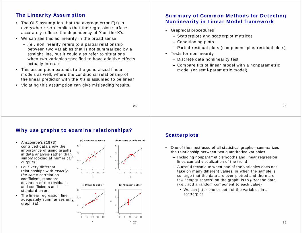
Why use graphs to examine relationships?

• Anscombe’s (1973) contrived data show the importance of using graphs in data analysis rather than simply looking at numericaloutputs

• Four very different relationships with exactly the same correlation coefficient, standard deviation of the residuals, and coefficients and standard errors

• The linear regression line adequately summarizes only graph (a)

0 5 10 15 20

05

1015

(a) Accurate summary

X

Y

0 5 10 15 20

05

1015

(b) Distorts curvilinear rel.

X

Y

0 5 10 15 20

05

1015

(c) Drawn to outlier

X

Y

0 5 10 15 20

05

1015

(d) "Chases" outlier

X

Y

28

Scatterplots

• One of the most used of all statistical graphs—summarizes the relationship between two quantitative variables– Including nonparametic smooths and linear regression

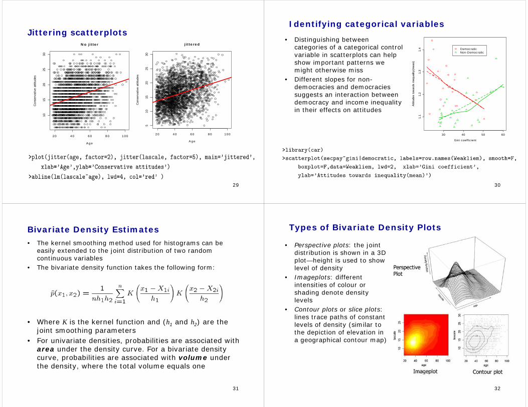
lines can aid visualization of the trend– A useful technique when one of the variables does not

take on many different values, or when the sample is so large that the data are over-plotted and there are few “empty spaces” on the graph, is to jitter the data (i.e., add a random component to each value)

• We can jitter one or both of the variables in a scatterplot

29

Jittering scatterplots

2 0 4 0 6 0 8 0 1 0 0

1015

2025

30N o j i t te r

A g e

Con

serv

ativ

e at

titud

es

2 0 4 0 6 0 8 0 1 0 0

510

1520

2530

j i t te re d

A g eC

onse

rvat

ive

attit

udes

30

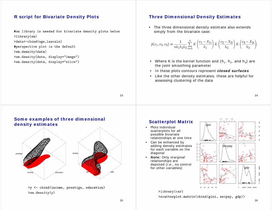
Identifying categorical variables

• Distinguishing between categories of a categorical control variable in scatterplots can help show important patterns we might otherwise miss

• Different slopes for non-democracies and democracies suggests an interaction between democracy and income inequality in their effects on attitudes

30 40 50 60

1.1

1.2

1.3

1.4

Gini coeffic ient

Attit

udes

tow

ards

ineq

ualit

y(m

ean)

DemocraticNon-Democratic

31

Bivariate Density Estimates• The kernel smoothing method used for histograms can be

easily extended to the joint distribution of two random continuous variables

• The bivariate density function takes the following form:

• Where K is the kernel function and (h1 and h2) are the joint smoothing parameters

• For univariate densities, probabilities are associated with area under the density curve. For a bivariate density curve, probabilities are associated with volume under the density, where the total volume equals one

32

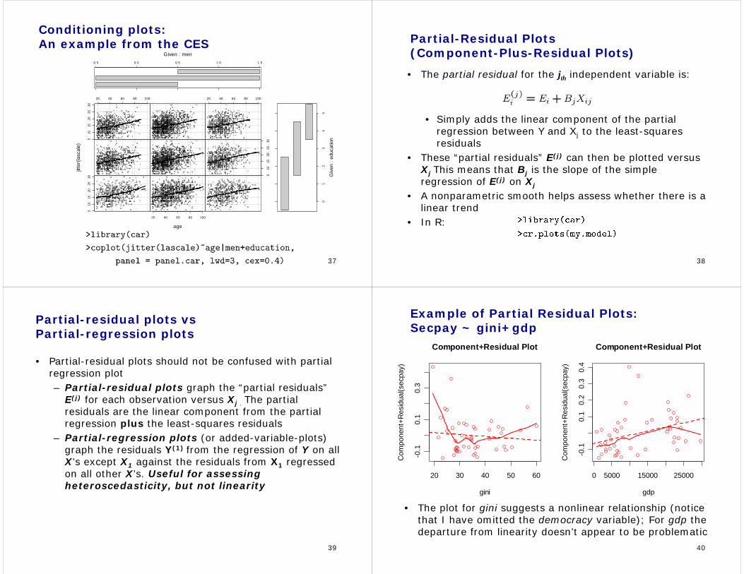
Types of Bivariate Density Plots

• Perspective plots: the joint distribution is shown in a 3D plot—height is used to show level of density

• Imageplots: different intensities of colour or shading denote density levels

• Contour plots or slice plots: lines trace paths of constant levels of density (similar to the depiction of elevation in a geographical contour map)

33

R script for Bivariate Density Plots

34

Three Dimensional Density Estimates

• The three dimensional density estimate also extends simply from the bivariate case:

• Where K is the kernel function and (h1, h2, and h3) are the joint smoothing parameter

• In these plots contours represent closed surfaces• Like the other density estimates, these are helpful for

assessing clustering of the data

35

Some examples of three dimensional density estimates

income

prestige

education gini

secpay

gdp

36

Scatterplot Matrix• Plots individual

scatterplots for all possible bivariaterelationships at one time

• Can be enhanced by adding density estimates for each variable on the diagonal

• Note: Only marginal relationships are depicted (i.e., no control for other variables)

||| ||| | | |||| || |||| | || |||| ||| || || ||| | |||||| | || ||||

gini

1.1 1.3 1.5

2030

4050

60

1.1

1.2

1.3

1.4

1.5

1.6

||| | || ||||| ||| | |||| || || | || |||| || |||| || | | ||||||| | |

secpay

20 30 40 50 60 0 10000 20000 30000

050

0015

000

2500

0

|| || | ||| | |||| | | ||| ||| ||| | |||| | | |||| || ||| ||||| || | |

gdp

37

Conditioning plots:An example from the CES

510

1520

2530

20 40 60 80 100

510

1520

2530

20 40 60 80 100

510

1520

2530

20 40 60 80 100

age

jitte

r(la

scal

e)

-0.5 0.0 0.5 1.0 1.5

Given : men

01

23

45

Giv

en :

educ

atio

n

38

Partial-Residual Plots(Component-Plus-Residual Plots)

• The partial residual for the jth independent variable is:

• Simply adds the linear component of the partial regression between Y and Xj to the least-squares residuals

• These “partial residuals” E(j) can then be plotted versus Xj This means that Bj is the slope of the simple regression of E(j) on Xj

• A nonparametric smooth helps assess whether there is a linear trend

• In R:

39

Partial-residual plots vsPartial-regression plots

• Partial-residual plots should not be confused with partial regression plot– Partial-residual plots graph the “partial residuals”

E(j) for each observation versus Xj . The partial residuals are the linear component from the partial regression plus the least-squares residuals

– Partial-regression plots (or added-variable-plots) graph the residuals Y(1) from the regression of Y on all X’s except X1 against the residuals from X1 regressed on all other X’s. Useful for assessing heteroscedasticity, but not linearity

40

Example of Partial Residual Plots:Secpay ~ gini+gdp

• The plot for gini suggests a nonlinear relationship (notice that I have omitted the democracy variable); For gdp the departure from linearity doesn’t appear to be problematic

20 30 40 50 60

-0.1

0.1

0.3

Component+Residual Plot

gini

Com

pone

nt+R

esid

ual(s

ecpa

y)

0 5000 15000 25000

-0.1

0.1

0.2

0.3

0.4

Component+Residual Plot

gdp

Com

pone

nt+R

esid

ual(s

ecpa

y)

41

Testing for Nonlinearity: Nested models and discrete data (1)

• A “lack of fit” test for nonlinearity is straightforward when the X variable of interest can be easily divided into discrete groups

• Essentially the goal is to categorize an otherwise quantitative explanatory variable, include it in a model replacing the original variable, and compare the fit of the two models

• This is done within a nested model framework, using an incremental F-test to determine the adequacy of the linear fit

• Of course, this lack of fit test is not viable when the X of interest takes on infinite possible values

42

Testing for Nonlinearity: Nested models and discrete data (2)

• Assume a model with one explanatory variable X that takes on 10 discrete values:

• We could refit this model treating X as a categorical variable, and thus employing a set of 9 dummy regressors:

• Model (A), which specifies a linear trend, is a special case of model (B), which captures any pattern of relationship between the E(Y) and X. In other words, model A is nested within model B

• If the linear model adequately captures the relationship, an incremental F-test will show that the difference between the two models is not be statistically significant

43

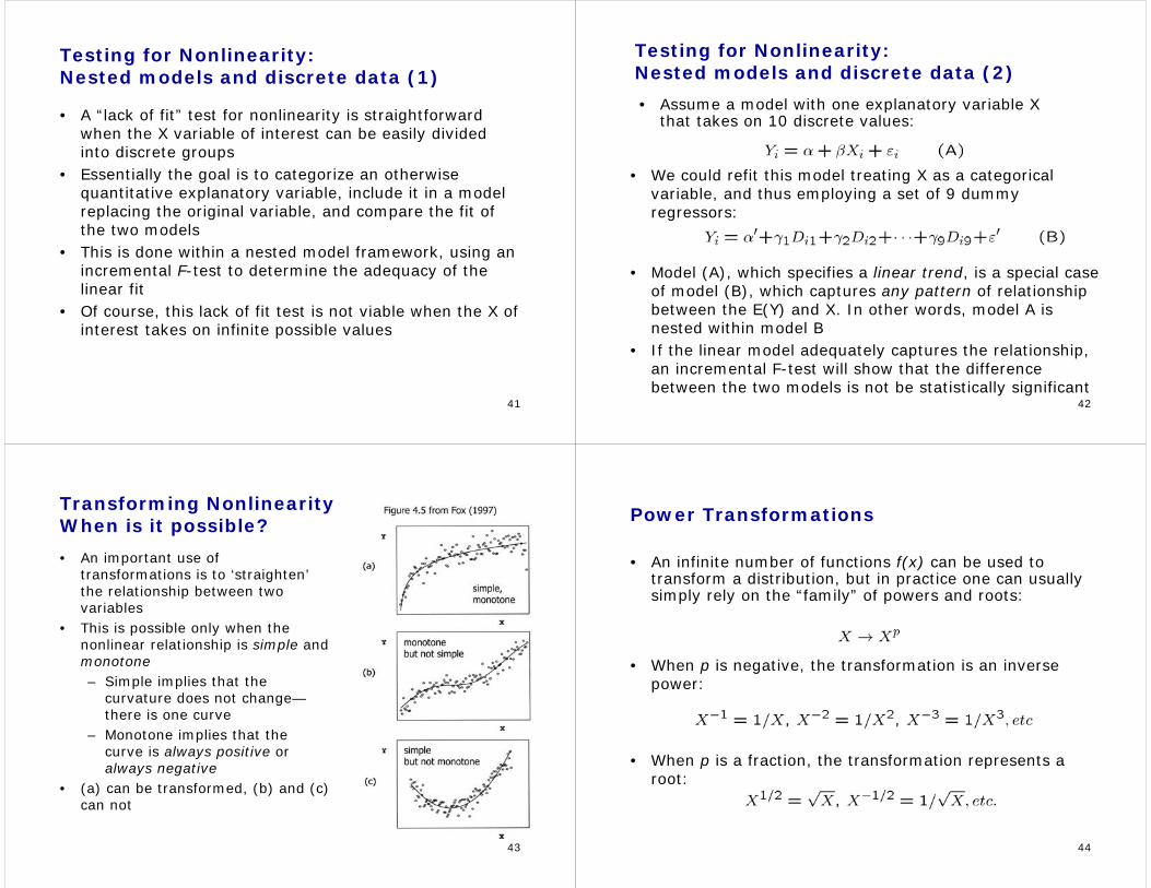
Transforming NonlinearityWhen is it possible?

• An important use of transformations is to ‘straighten’the relationship between two variables

• This is possible only when the nonlinear relationship is simple and monotone– Simple implies that the

curvature does not change—there is one curve

– Monotone implies that the curve is always positive oralways negative

• (a) can be transformed, (b) and (c) can not

44

Power Transformations

• An infinite number of functions f(x) can be used to transform a distribution, but in practice one can usually simply rely on the “family” of powers and roots:

• When p is negative, the transformation is an inverse power:

• When p is a fraction, the transformation represents a root:

45

Log Transformations

• A power transformation of X0 is useless because it changes all values to 1 (i.e., it makes the variable a constant)

• Instead we can think of X0 as a shorthand for the log transformation logeX, where e=2.718 is the base of the natural logarithms:

• In terms of result, it matters little which base is used for a log transformation because changing base is equivalent to multiplying X by a constant

46

A few notes on Power Transformations1. Descending the ladder of powers and roots

compresses the large values of X and spreads out the small values

2. As p moves away from 1 in either direction, the transformation becomes more powerful

3. Power transformations are sensible only when all the X values are positive—If not, this can be solved by adding a start value– Some transformations (e.g., log, square root, are

undefined for 0 and negative numbers)– Other power transformations will not be

monotone, thus changing the order of the data

47

‘Bulging Rule’ for Transformations(Tukey and Mosteller)

• Normally we should try to transform explanatory variables rather than the response variable Y – A transformation of Y

will affect the relationship of Y with all Xs, not just the one with the nonlinear relationship

• If, however, the response variable is highly skewed, it can make sense to transform it instead (e.g., income)

48

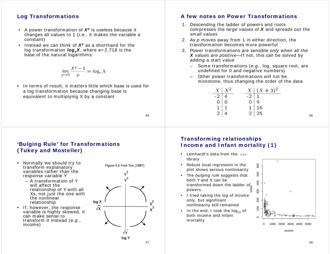
Transforming relationshipsIncome and Infant mortality (1)

• Leinhardt’s data from the carlibrary

• Robust local regression in the plot shows serious nonlinearity

• The bulging rule suggests that both Y and X can be transformed down the ladder of powers

• I tried taking the log of income only, but significant nonlinearity still remained

• In the end, I took the log10 of both income and infant mortality

0 1000 2000 3000 4000 5000

010

020

030

040

050

060

0

income

infa

nt

49

Income and Infant mortality (2)

2.0 2.5 3.0 3.5

1.0

1.5

2.0

2.5

log.income

log.

infa

nt

• A linear model fits well here

• Since both variables are transformed by the log10 the coefficients are easy to interpret:– An increase in

income by 1% is associated, on average, with a .51% decrease in infant mortality

50

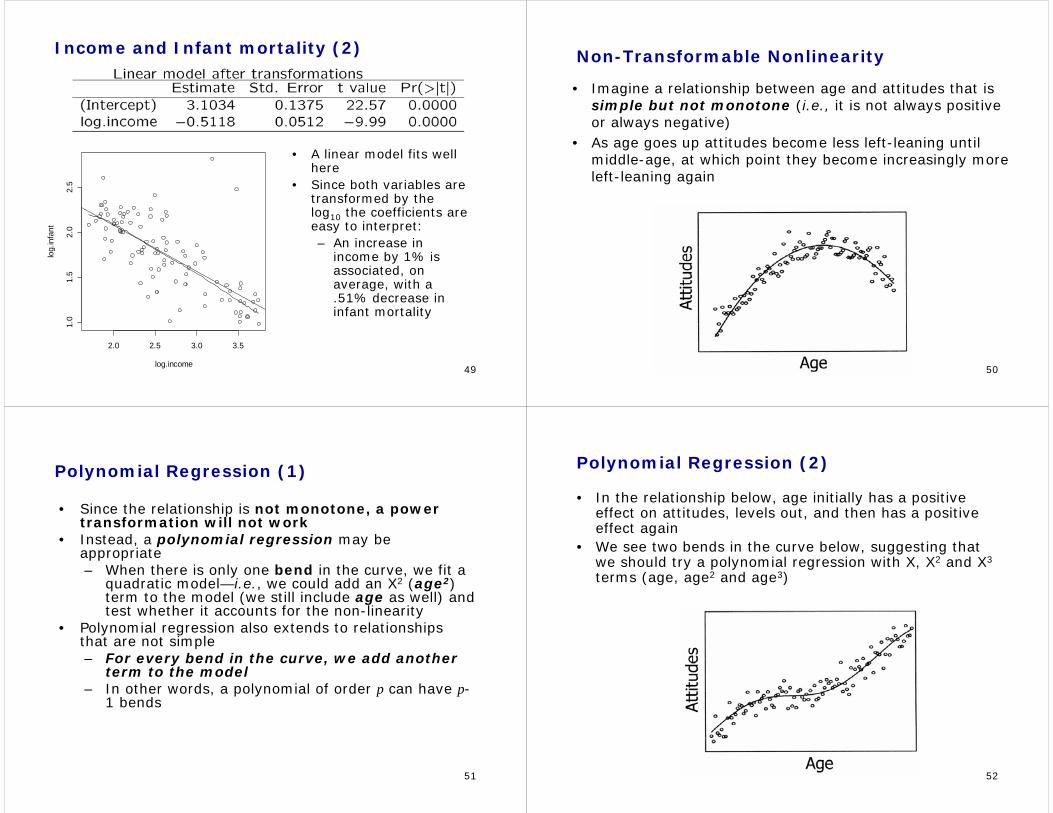
Non-Transformable Nonlinearity

• Imagine a relationship between age and attitudes that is simple but not monotone (i.e., it is not always positive or always negative)

• As age goes up attitudes become less left-leaning until middle-age, at which point they become increasingly more left-leaning again

51

Polynomial Regression (1)

• Since the relationship is not monotone, a power transformation will not work

• Instead, a polynomial regression may be appropriate– When there is only one bend in the curve, we fit a

quadratic model—i.e., we could add an X2 (age2) term to the model (we still include age as well) and test whether it accounts for the non-linearity

• Polynomial regression also extends to relationships that are not simple– For every bend in the curve, we add another

term to the model– In other words, a polynomial of order p can have p-

1 bends

52

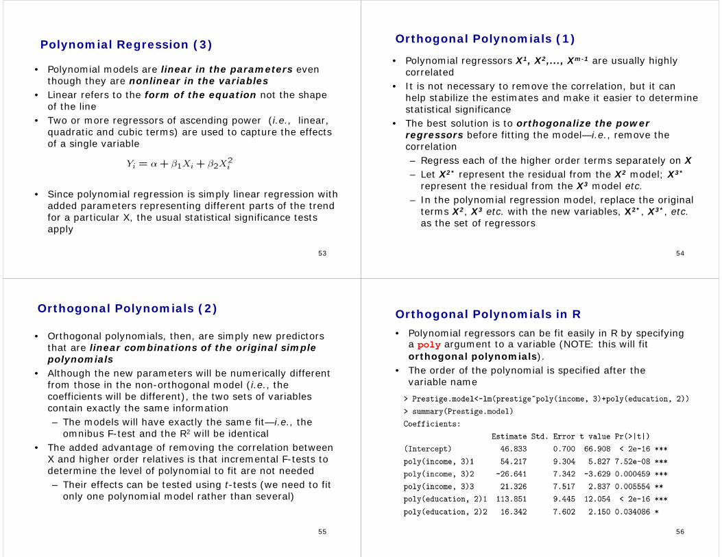
• In the relationship below, age initially has a positive effect on attitudes, levels out, and then has a positive effect again

• We see two bends in the curve below, suggesting that we should try a polynomial regression with X, X2 and X3

terms (age, age2 and age3)

Polynomial Regression (2)

53

• Polynomial models are linear in the parameters even though they are nonlinear in the variables

• Linear refers to the form of the equation not the shape of the line

• Two or more regressors of ascending power (i.e., linear, quadratic and cubic terms) are used to capture the effects of a single variable

• Since polynomial regression is simply linear regression with added parameters representing different parts of the trend for a particular X, the usual statistical significance tests apply

Polynomial Regression (3)

54

Orthogonal Polynomials (1)

• Polynomial regressors X1, X2,..., Xm-1 are usually highly correlated

• It is not necessary to remove the correlation, but it can help stabilize the estimates and make it easier to determine statistical significance

• The best solution is to orthogonalize the power regressors before fitting the model—i.e., remove the correlation– Regress each of the higher order terms separately on X– Let X2* represent the residual from the X2 model; X3*

represent the residual from the X3 model etc.– In the polynomial regression model, replace the original

terms X2, X3 etc. with the new variables, X2*, X3*, etc.as the set of regressors

55

Orthogonal Polynomials (2)

• Orthogonal polynomials, then, are simply new predictors that are linear combinations of the original simple polynomials

• Although the new parameters will be numerically different from those in the non-orthogonal model (i.e., the coefficients will be different), the two sets of variables contain exactly the same information– The models will have exactly the same fit—i.e., the

omnibus F-test and the R2 will be identical• The added advantage of removing the correlation between

X and higher order relatives is that incremental F-tests to determine the level of polynomial to fit are not needed– Their effects can be tested using t-tests (we need to fit

only one polynomial model rather than several)

56

Orthogonal Polynomials in R

• Polynomial regressors can be fit easily in R by specifying a poly argument to a variable (NOTE: this will fit orthogonal polynomials).

• The order of the polynomial is specified after the variable name

57

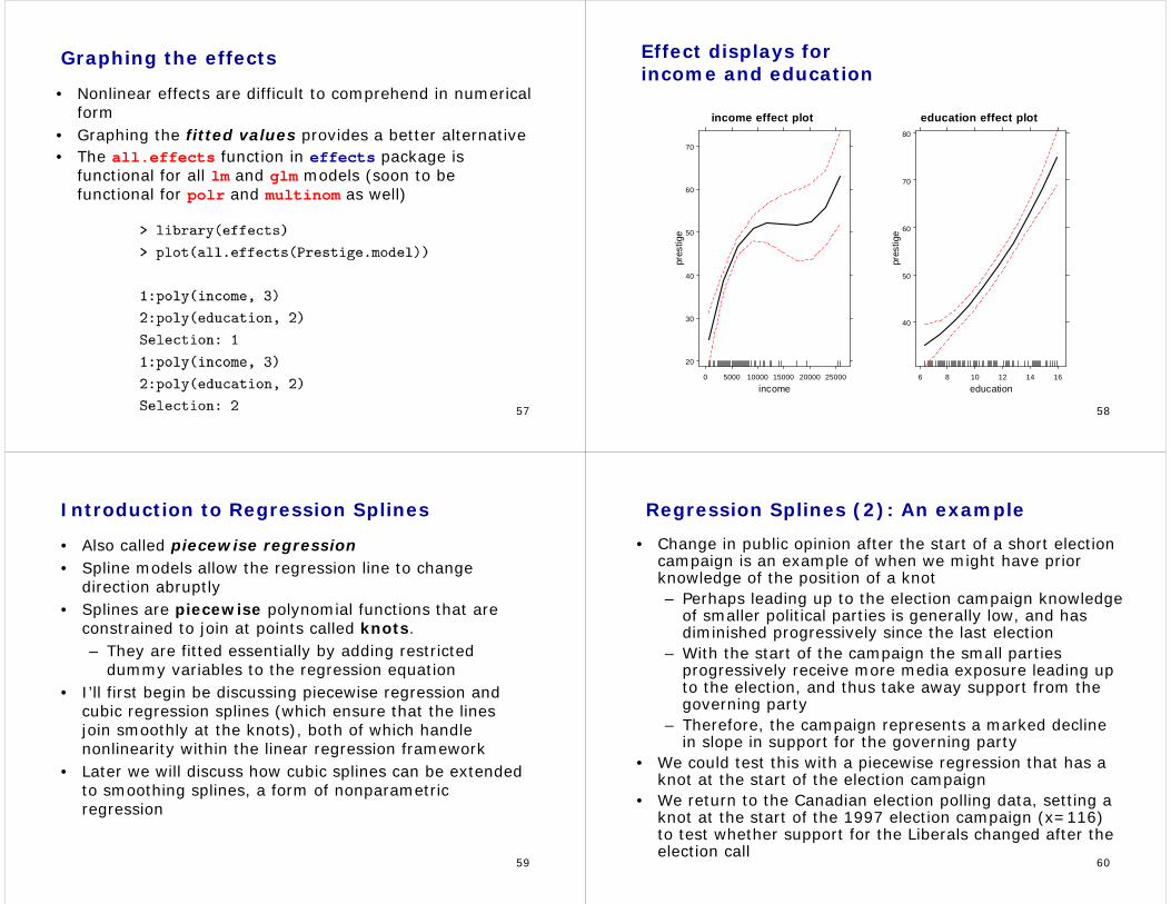
Graphing the effects

• Nonlinear effects are difficult to comprehend in numerical form

• Graphing the fitted values provides a better alternative• The all.effects function in effects package is

functional for all lm and glm models (soon to be functional for polr and multinom as well)

58

Effect displays for income and education

income effect plot

income

pres

tige

20

30

40

50

60

70

0 5000 10000 15000 20000 25000

education effect plot

education

pres

tige

40

50

60

70

80

6 8 10 12 14 16

59

Introduction to Regression Splines

• Also called piecewise regression• Spline models allow the regression line to change

direction abruptly• Splines are piecewise polynomial functions that are

constrained to join at points called knots.– They are fitted essentially by adding restricted

dummy variables to the regression equation• I’ll first begin be discussing piecewise regression and

cubic regression splines (which ensure that the lines join smoothly at the knots), both of which handle nonlinearity within the linear regression framework

• Later we will discuss how cubic splines can be extended to smoothing splines, a form of nonparametric regression

60

Regression Splines (2): An example

• Change in public opinion after the start of a short election campaign is an example of when we might have prior knowledge of the position of a knot– Perhaps leading up to the election campaign knowledge

of smaller political parties is generally low, and has diminished progressively since the last election

– With the start of the campaign the small parties progressively receive more media exposure leading up to the election, and thus take away support from the governing party

– Therefore, the campaign represents a marked decline in slope in support for the governing party

• We could test this with a piecewise regression that has a knot at the start of the election campaign

• We return to the Canadian election polling data, setting a knot at the start of the 1997 election campaign (x=116) to test whether support for the Liberals changed after the election call

61

Regression Splines (3)

• In order to set the intercept at the knot, I start by defining two basis functions, one for polls taking place before the start of the election (X=116) and another for polls conducted after the start of the election campaign

• I then simply fit a regular linear model including the two basis functions:

62

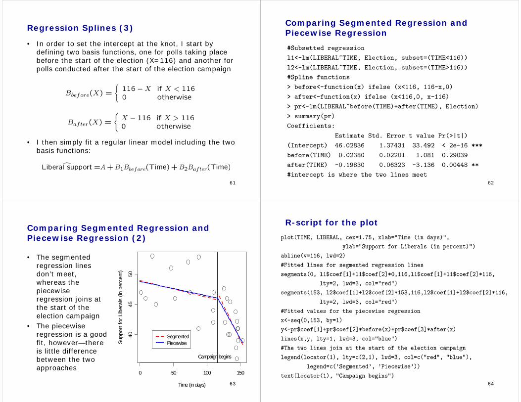
Comparing Segmented Regression and Piecewise Regression

63

Comparing Segmented Regression and Piecewise Regression (2)

• The segmented regression lines don’t meet, whereas the piecewise regression joins at the start of the election campaign

• The piecewise regression is a good fit, however—there is little difference between the two approaches

0 50 100 150

4045

50

Time (in days)

Supp

ort f

or L

iber

als

(in p

erce

nt)

SegmentedPiecewise

Campaign begins

64

R-script for the plot

65

Cubic Splines

• Cubic splines combine polynomial regression and piecewise regression by representing the trend as a set of piecewise polynomials joined at knots

• Not as smooth as global polynomial regression—where each point affects the global fit—but generally behave much better at the peaks

• Also better able to handle more complicated patterns of nonlinearity than polynomial regression

• Must consideration the (1) number of regions; (2) degree of polynomial; and (3) location of the knots– For most theoretical questions, we are not sure where

the knots should be. – Fortunately, it turns out that as long as the knots are

evenly spaced, the only thing that really matters is the number of knots.

66

Cubic Splines (2)Number and Position of Knots

• Equally spaced fixed knots ensures that there is enough data within each region X to get a sensible fit– It also guards against outliers overly influencing the

curve• Typically a choice of 3< k < 7 works well, and more than

5 knots is seldom necessary– For large samples sizes (n≥100) with a continuous

response variable, k=5 usually provides a good compromise between flexibility and loss of precision

– For small samples (<30) k=3 is a good starting point• Akaike’s Information Criterion (AIC) can be used for

a data-based selection of k– The value of k that gives the lowest AIC can then be

selected

67

Cubic Splines in R• As was the case for the piecewise regression, cubic

splines can be implemented by manually creating basis functions

• Alternatively, they can be implemented using the splinespackage for R:– Cubic B-Splines are specified using the bs(variable) argument for the lm function

– Natural Cubic Splines are fit using the ns(variable) argument for the lm function

• For both functions, either the degrees of freedom or the number of knots can be chosen—By default, no knots are specified, meaning that a regular polynomial is fit– For bs df-degree-1=knots are specified when df is given– For ns, if the df are specified, df-1–intercept=evenly

spaced knots are specified

68

Complicated Nonlinearity

• Transformations work well when the nonlinear pattern is simple and monotone. They should not be used otherwise, however.

• Polynomial regression is an excellent method to model nonlinearity that is neither simple nor monotone but this method works well only to a certain level of complexity– If the trend takes too many turns in direction,

polynomial regression typically does a poor job of representing the trend, especially at the peaks

– I recommend that a cubic regression (X, X2, X3) is the highest level polynomial one uses

• We thus need another method to model more complicated nonlinear patterns. This leads us to nonparametric regression and a more general way to think of regression.

69

Lunch Break