THE MORE WE DIE, THE MORE WE SELL?A SIMPLE TEST OF THE HOME-MARKET

EFFECT*

Arnaud Costinot

Dave Donaldson

Margaret Kyle

Heidi Williams

December 2018

Abstract

The home-market effect, first hypothesized by Linder (1961) and later formalized

by Krugman (1980), is the idea that countries with larger demand for some products

at home tend to have larger sales of the same products abroad. In this paper, we de-

velop a simple test of the home-market effect using detailed drug sales data from the

global pharmaceutical industry. The core of our empirical strategy is the observation

that a country’s exogenous demographic composition can be used as a predictor of

the diseases that its inhabitants are most likely to die from and, in turn, the drugs

that they are most likely to demand. We find that the correlation between predicted

home demand and sales abroad is positive and greater than the correlation between

predicted home demand and purchases from abroad. In short, countries tend to be

net sellers of the drugs that they demand the most, as predicted by Linder (1961) and

Krugman (1980). JEL Codes: F1, O3.

*We are very grateful to Manon Costinot, Maya Durvasula, Masao Fukui, Ryan Hill, Anton Popov, JuanRios, Oliver Salzmann, Mahnum Shahzad, and Sophie Sun for excellent research assistance, as well as toDaron Acemoglu, Pol Antràs, David Atkin, Keith Head, David Weinstein, three anonymous referees, andseminar audiences at many institutions for comments that have improved this work. We thank PierreAzoulay, Joshua Graff Zivin, Danielle Li, and Bhaven Sampat for sharing advice and data on the NIHsubsidy analysis presented in this paper. The construction of some of the data analyzed in this publicationwas supported by the National Institute on Aging and the NIH Common Fund, Office of the NIH Director,through Grant U01-AG046708 to the National Bureau of Economic Research (NBER); the content is solelythe responsibility of the authors and does not necessarily represent the official views of the NIH or NBER.Financial support from NSF Grant Number 1151497, the Hoover IP2 working group, and the IntellectualProperty and Markets for Technology Chair at MINES ParisTech is also gratefully acknowledged. Kylethanks Pfizer for access to the IMS data used. Corresponding author: Donaldson; MIT Department ofEconomics; 50 Memorial Drive; E52-554; Cambridge MA 02142; ddonald@mit.edu. Word Count: 16776.

1

I INTRODUCTION

Do countries with larger domestic markets for some products tend to sell more of thosesame products in foreign markets? The idea that local demand may stimulate exportsis an old one. First hypothesized by Linder (1961) and later formalized by Krugman(1980), the so-called home-market effect has become a central tenet of the new trade the-ory (Helpman and Krugman, 1985, 1989) and the new economic geography literature (Fu-jita et al., 2001). In terms of policy, it implies that import protection may be used as exportpromotion, a view often more popular in business communities than among economists(Krugman, 1984).

To establish the empirical validity of the home-market effect, one must overcome a keychallenge. While theory predicts that the cross-sectional variation in demand causes thepattern of international specialization, observable demand shifters are rarely available inpractice. National accounts, for instance, may report how much a country spends on aparticular good. But expenditures depend on prices, which themselves depend on supply,not just on demand conditions.

In this paper, we propose a simple test of the home-market effect that uses variation indisease burdens across countries as a way to address this empirical challenge. Our start-ing point is the observation by Acemoglu and Linn (2004) that demographic groups whoare more likely to die from particular diseases—because of exogenous characteristics—arealso more likely to demand pharmaceutical treatments that target those diseases. In theiroriginal paper, Acemoglu and Linn (2004) exploit such demographic variation over timewithin the United States to estimate the impact of market size on innovation. Here, weemploy the spatial analog of this strategy, drawing on cross-sectional variation in the de-mographic composition of different countries in a given year, to explore how exogenousvariation in demand may shape the pattern of trade.

Intuitively, our empirical strategy exploits the twin facts that disease burdens varyby demographic groups, and that countries vary in their demographic composition, toconstruct a “predicted disease burden” measure for each disease in each country in agiven year, which measures the average country-level disease burden that would be ex-pected given a country’s demographic structure. Using this measure, we can then testfor the existence of the home-market effect by estimating (i) whether higher (predicted)disease burdens at home tend to increase the sales of domestic drugs treating those dis-eases abroad (what we term the weak home-market effect), and if so, (ii) whether they tendto increase them by more than the sales of foreign drugs at home (our strong home-marketeffect).

1

To take a concrete example, consider the drug famotidine (known as Pepcid® in theUnited States). Famotidine is used to treat peptic ulcers and gastro-esophageal reflux,and was discovered in Japan (Hara, 2003)—a country known for particularly high inci-dence rates of peptic ulcers. In our data, individuals in Japan are nearly twice as likelyto die from digestive disorders than are individuals in the rest of the world (0.266 deathsper 1,000 population annually in Japan, relative to 0.170 on average in other countries).Looking at data on Japan’s exports and imports, sales of Japanese drugs targeting pepticulcers and gastro-esophageal reflux diseases outside Japan account for 10.35% of worldsales, compared to an average of 4.54% for all other disease categories. More strikingly,Japan is a net importer in the pharmaceutical sector as a whole, but is a net exporter ofdrugs targeting peptic ulcers, reflux, and related digestive diseases.

While the previous observation is consistent with the potential existence of the home-market effect, building an empirical paper around such examples is challenging for manyreasons. In this particular case, Cleave (1962) conjectures that Japan has higher rates ofpeptic ulcers due to differences in dietary consumption (namely, higher consumption ofsalty foods), but cross-country variation in diets could at least in part reflect differencesin relative prices, and hence supply considerations. Our empirical strategy, based on thetype of demographic variation exploited by Acemoglu and Linn (2004), is designed toaddress such endogeneity issues.1

The rest of our paper is organized as follows. After discussing the related literaturein Section II, we present a flexible model of the supply and demand for pharmaceuticaldrugs in Section III. For expositional purposes, we first study a perfectly competitiveenvironment. In this context, we introduce a simple test of the weak and strong home-market effects based on a log-linear approximation of our model around a symmetricequilibrium and characterize the conditions for such effects to arise. We then show thatthe same test remains valid in a range of imperfectly competitive environments, includingthe one considered in Krugman (1980). Our theoretical analysis highlights the role ofsector-level economies of scale, while clarifying that their particular determinants may beirrelevant for the validity of our test.

Section IV describes our data. Our empirical analysis draws on a linkage between twodatasets. The first one documents sales in 56 countries of more than 20,000 molecules byroughly 2,650 firms, which we convert to a dataset of bilateral sales at the disease level, bymatching each firm to the country in which it is headquartered and each molecule to thedisease that it targets.2 The second dataset documents the demographic composition of

1Other applications of this strategy can be found in DellaVigna and Pollet (2007) and Jaravel (2018).2Our dataset does not contain information about location of production. Thus, we cannot shed light

2

and disease burdens in the same 56 countries, which we use to compute predicted diseaseburdens by country and disease.

Section V presents our main results. Our simple test focuses on a log-linear specifica-tion where bilateral sales of drugs targeting different diseases are allowed to depend on(i) disease burdens in the destination country, i.e., the country where drugs are sold; (ii)disease burdens in the origin country, i.e., the country where firms selling those drugs areheadquartered; and (iii) a full vector of disease indicator variables and destination-and-origin indicator variables. Everything else equal, we document that countries tend to sellrelatively more of the drugs for which they have higher disease burdens, in line with theexistence of a weak home-market effect. Furthermore, the elasticity of sales towards for-eign countries tends to be higher than the elasticity of purchases from foreign countries,consistent with the existence of a strong home-market effect.

Section VI analyzes further the economic determinants of the home-market effect.While the previous results provide empirical support for the notion of a home-market ef-fect in the global pharmaceutical sector, the existence and magnitude of this phenomenondepend, according to our model, on both demand and supply elasticities. Our last resultspoint towards the home-market effect being driven by substantial economies of scale atthe sector-level rather than low elasticities of demand. Quantitatively, the sector-leveleconomies of scale that we estimate in the pharmaceutical industry are about 25% smallerthan those that Krugman’s (1980) monopolistically competitive model predicts.

II RELATED LITERATURE

The literature on the home-market effect is large and varied. As we explain below, thevariation derives in part from the use of related, but distinct, definitions of “the” home-market effect by different authors.

Whereas both Linder’s (1961) and Krugman’s (1980) original work emphasize the con-sequences of cross-country differences in demand for the pattern of trade, Helpman andKrugman (1985) focus instead on whether larger countries tend to specialize in sectorswith larger economies of scale.3 Subsequent work by Davis (1998), Head et al. (2002),Holmes and Stevens (2005), and Behrens et al. (2009) provide additional conditions onthe nature of trade costs as well as the number of goods and countries under which thelatter pattern may or may not arise. Amiti (1998), in turn, studies whether larger countries

on whether the home-market effect ultimately operates through exports, foreign direct investment, or amixture of both. We come back to this point when discussing the related literature in Section II.

3Ethier (1982) discusses similar issues in a perfectly competitive model with external economies of scale.

3

should have a comparative advantage in sectors with higher trade costs. Motivated by thetheoretical predictions of Helpman and Krugman (1985), Hanson and Xiang (2004) showthat high-GDP countries tend to sell disproportionately more in sectors with larger trans-portation costs and lower elasticities of substitution, a measure of sector-level economiesof scale under monopolistic competition. In related work, Feenstra et al. (2001) documentthat high-GDP countries tend to be net exporters of differentiated goods, which they alsointerpret as evidence of a home-market effect in such industries.4

A number of more recent theoretical papers have extended the work of Krugman(1980) to study the implications of non-homothetic preferences for the pattern of tradeand foreign direct investment; see Fajgelbaum et al. (2011, 2015) and Matsuyama (2015). Akey prediction of these models is that in the presence of economies of scale, rich countriesthat have larger demand for high-quality goods will tend to specialize in those goods. Asa result, they will trade more with, or invest more in, other rich countries, as also empha-sized by Linder (1961). In these models, exogenous differences in income across countriesplay the same role as differences in preferences in Krugman (1980). In line with the previ-ous models, Caron et al. (2015) document that the sectors on which high-GDP countriesspend more also tend to be the sectors in which high-GDP countries export more. Din-gel (2016) also offers empirical evidence consistent with the previous mechanism usinginformation about shipment prices from different U.S. cities and the income compositionof neighboring cities.

Our analysis is most closely related to the early empirical work of Davis and Weinstein(1996) and later studies by Davis and Weinstein (1999, 2003), Lundback and Torstensson(1998), Head and Ries (2001), Trionfetti (2001), Weder (2003), Crozet and Trionfetti (2008),and Brulhart and Trionfetti (2009). Like ours, the aforementioned papers focus on theimpact of differences in demand on the pattern of international specialization. In theirreview of the literature, Head and Mayer (2004) conclude that this type of empirical ev-idence on the home-market effect is highly mixed.5 While empirical specifications anddata sources vary across studies, the previous papers all share one key characteristic:

4Provided that the economy is subject to increasing returns to scale, one would also expect larger coun-tries to have higher wages. In their survey of the literature, Head and Mayer (2004) refer to this predictionas the “price” aspect of the home-market effect. Though our analysis implicitly allows for such effects tobe active, it focuses exclusively on the relationship between economies of scale, cross-country demand dif-ferences, and international specialization. This is what Head and Mayer (2004) refer to as the “quantity”aspect of the home-market effect.

5Given our focus on the pharmaceutical industry, it is worth nothing that Trionfetti’s (2001) sector-leveltest for the home-market effect is rejected for “Chemical Products.” Fabrizio and Thomas (2012) provideanother estimate that is specific to the pharmaceutical industry. They document that pharmaceutical firms’patenting is more correlated with home sales (and cultural proxies for home sales) than with foreign sales,thus suggesting a systematic relationship between home demand and firm-level innovation.

4

data on expenditure shares are used as a proxies for demand differences. As argued ear-lier, one non-trivial issue with such proxies is that differences in local supply conditionsmay also affect expenditure shares through their effects on local prices. This makes earliertests of the home-market effect hard to interpret.

Compared to earlier work on the home-market effect, we view the approach in thispaper as having both costs and benefits. Since the home-market effect emphasized byLinder (1961) and Krugman (1980) is about the causal effect of demand differences acrosscountries, any test of this effect ultimately requires exogenous demand variation. Whilewe have no silver bullet to deal with endogeneity issues, and we discuss the challengesassociated with our approach later in the paper, we believe that using (predicted) diseaseburdens as observable demand shifters rather than expenditure shares is a significant stepforward.

A first drawback of our empirical strategy is that its scope is restricted to an impor-tant, but single, industry.6 Another limitation of our dataset is that it does not allow us todistinguish between exports and foreign direct investment: we only observe total sales byfirms headquartered in a particular country. Thus, the home-market effect that we iden-tify may operate through both exports and foreign direct investment, not just exports ashas been emphasized in the previous literature. The previous observation notwithstand-ing, it is not clear that if the only choice were to study either exports or the sum of exportsand sales by foreign affiliates, one should prefer the former to the latter since the sameeconomic forces are likely to be at play for both types of sales.

III THE SIMPLE ECONOMICS OF THE HOME MARKET

EFFECT

We begin with a theoretical analysis that is split into two steps. First, we consider a worldeconomy with perfect competition (Section III.1) and develop a test of the home-marketeffect in this environment (Section III.2). This allows us to describe the logic of the home-market effect in the simplest possible way using supply and demand analysis. Second,we demonstrate how our test of the home-market effect and its economic interpretationmay carry over to industries with imperfect competition, endogenous innovation, and

6According to the World Trade Organization, global exports in the pharmaceutical industry grew fasterbetween 1995 and 2014 than in any other besides fuel, surpassing $500 billion (or approximately threepercent of global merchandise trade) by 2014. The pharmaceutical sector has also received considerableattention in recent trade agreements, particularly the Agreement on Trade-Related Aspects of IntellectualProperty Rights (TRIPS) and the Trans-Pacific Partnership (TPP).

5

price regulations (Section III.3). This illustrates the broader applicability of our empiricalstrategy and justifies using data from the pharmaceutical industry to implement our testin subsequent sections.

III.1 Perfectly Competitive Benchmark

Demand. To facilitate the connection between our theoretical and empirical analysis,we focus on an economy where individuals consume drugs that target multiple diseases,indexed by n, as well as other goods, which we leave unspecified. Empirically, eachdisease n will correspond to a broad disease class like “cardiovascular diseases.” Weassume that the aggregate consumption of drugs targeting disease n in country j can beexpressed as

(1) Dnj = θn

j D(Pnj /Pj)Dj,

where D(·) is a strictly decreasing function; Pnj depends on the prices of drugs targeting

disease n in country j, as described below; Dj and Pj are endogenous country-specificdemand shifters that are common to all drugs in country j; and θn

j is an exogenous disease-and-country-specific demand shifter, which we will later measure using data on diseaseburdens.

Within each disease category n, drugs may be purchased from different countries.Any of these countries may be producing different versions of the same molecule (e.g.generic versus non-generic), different molecules targeting the same narrow disease (e.g.angiotensin II receptor blockers and beta blockers, both treatments for high blood pres-sure, a risk factor for hypertensive heart disease), or different molecules targeting dif-ferent diseases within the same broad category (e.g. drugs targeting hypertensive heartdisease vs. coronary artery disease, within the broad category of cardiovascular diseases).The previous considerations suggest imperfect substitutability between drugs from dif-ferent countries, which we capture through the following specification,

(2) dnij = d(pn

ij/Pnj )Dn

j ,

where d(·) is a strictly decreasing function; dnij denotes country j’s consumption of vari-

eties from country i targeting disease n, pnij denotes the consumer price for these varieties,

and Pnj is implicitly defined by the solution to

(3) Pnj = ∑ pn

ijd(pnij/Pn

j ).

6

Given the level of aggregation in our empirical analysis, pnij should itself be interpreted

as a price index, aggregating prices across all firms from country i selling drugs targetingdisease n in country j. We will make this aggregation explicit in Sections III.3 and VI.1.7

Supply. Perfectly competitive firms produce up to the point at which drug prices areequal to marginal costs. For each disease n and country i, this leads to a supply curve,

(4) sni = ηn

i s(pni ),

where pni denotes the producer price of drugs targeting disease n in country i and ηn

i isa disease-and-country specific supply shifter, which may capture both technological andpolicy differences. Depending on whether there are external economies of scale or not,s(·) may be upward- or downward-sloping. Trade is subject to iceberg frictions. To sellone unit of a given drug to country j 6= i, firms from country i must ship τn

ij ≥ 1 units.8

Without loss of generality, we set τnii = 1 for all i and n. Non-arbitrage implies

(5) pnij = τn

ij pni .

Equilibrium. Supply equals demand for each drug,

(6) sni = ∑

jτn

ij dnij.

III.2 Weak and Strong Home-Market Effects

The home-market effect is the general idea that, everything else being equal, countriestend to sell more abroad in sectors for which they have larger domestic markets. Here,

7For the purposes of testing the home-market effect, we do not need the previous demand functions tobe consistent with the behavior of a representative agent in country j, an assumption that may be particu-larly strong in a sector where demand involves physicians, pharmacists, insurers, and patients. We note,however, that equations (1)-(3) are consistent with the common assumption of nested CES utility functions,which corresponds to the special case where D(·) and d(·) are power functions.

8Though we abstract from multinational production in our baseline model, equations (4) and (5) wouldstill hold in a world economy with multinational activities à la Ramondo and Rodríguez-Clare (2013) andexternal economies of scale at the level of the headquarter country for each disease. In such an environment,τn

ij would simply correspond to the minimum cost of accessing country j from country i, either through ex-ports or foreign direct investment; see Online Appendix A.1. Note also that while transport costs and tariffsare low in the pharmaceutical industry, drug sales exhibit significant home-bias. This is partly due to localregulations that act as non-tariff barriers; see Thomas (1994). For example, governments may favor domes-tic firms in granting approval or when negotiating prices. Iceberg trade costs in our baseline model aim tocapture all the frictions involved when selling pharmaceuticals in foreign markets that appear to persist,notwithstanding the adoption of free trade agreements and international efforts to harmonize regulations.

7

we operationalize this idea in the context of a log-linearized version of our model arounda symmetric equilibrium.

Defining Home-Market Effects. Let us start by considering the bilateral sales, xnij ≡

pnijd

nij , of drugs targeting disease n by firms from country i in country j 6= i. Around a

symmetric equilibrium with trade costs, τ ≥ 1, and common demand and supply shocksacross countries and diseases, we can express bilateral sales, up to a first-order approxi-mation, as

(7) ln xnij = δij + δn + βM ln θn

j + βX ln θni + εn

ij,

where δij is an origin-destination-specific term that captures systematic determinants ofbilateral trade flows such as physical distance or whether countries i and j share the samelanguage; δn is a disease-specific term that captures worldwide variation in demand andsupply conditions across drugs targeting different diseases; βM is the elasticity of tradeflows with respect to demand shocks in the importing country; βX is the elasticity of tradeflows with respect to demand shocks in the exporting country j; and εn

ij is a residual thatcaptures idiosyncratic variation in trade costs and supply conditions.

Provided that demand shocks, supply shocks, and trade costs are close enough to theirvalues in a symmetric equilibrium, the previous elasticities can be mapped into the struc-tural parameters of Section III.1, as we do in Online Appendix A.2. The key benefit oflog-linearizing our model around a symmetric equilibrium is that we obtain elasticities,βM and βX, that have a structural interpretation—discussed in detail below—and are con-stant across origins, destinations, and diseases—which is appealing from an econometricstandpoint.9 The main drawback of our approach is that it assumes away differential ef-fects of demand in third countries, l 6= i, j, on the bilateral sales of country i in country j.In equation (7), the effects of demand in those countries is subsumed by the disease fixedeffect, δn, which is a function of ∑l θn

l . We come back to this point in Sections V.2 and VI.1.To motivate our definition of the home-market effect, and help relate our analysis to

earlier work in the literature, let us now go from bilateral to aggregate sales. Starting fromequation (7), we can express total exports, Xn

i ≡ ∑j 6=i xnij, and total imports, Mn

i ≡ ∑j 6=i xnji,

9For instance, if we were to log-linearize around an equilibrium where trade costs are identical acrossdiseases, but allowed to vary across country pairs, τn

ij ≡ τij, then the two elasticities in equation (7) wouldalso vary across country pairs, i.e, we would have βM,ij and βX,ij.

8

as

ln Xni = δn + βX ln θn

i + ln(∑j 6=i

(θnj )

βM exp(δij + εnij)),(8)

ln Mni = δn + βM ln θn

i + ln(∑j 6=i

(θnj )

βX exp(δji + εnji)).(9)

According to equation (8), a country tends to export more of the goods for which it haslarger domestic demand if and only if βX > 0. And according to equations (8) and (9), acountry tends to be a net exporter of the goods for which it has a larger domestic marketif and only if βX > βM.10 Based on these two observations, we propose the followingdefinition.

Definition. Trade flows satisfy the weak home-market effect if βX > 0 and the strong home-market effect if βX > βM.

This definition will be the basis of our empirical test of the home-market effect. Givendata on bilateral sales, {xn

ij}, and observable demand shifters, {θni }, we will estimate βX

and βM in equation (7) and test whether or not the two previous inequalities hold. Thissimple approach differs from earlier tests of the home-market effect in three importantrespects.

First, our empirical test has a structural interpretation, which is discussed below.Among other things, this allows one to discuss the origin of the error term in equation(7) and the extent to which one should expect the orthogonality condition to hold or not,important points that we come back to in Section V.2.

Second, and relatedly, our empirical test focuses on elasticities with respect to demandshocks, not expenditure shares. If preferences across sectors are Cobb-Douglas, the twoelasticities are equivalent. Away from this empirically knife-edge case, they are not. As-suming that observable demand shocks are available, a case that we make in Section IV,using these shocks alleviates concerns about “false positives”—that is, positive correla-tions between exports and expenditure shares driven by unobserved supply shocks thatare positively correlated with both exports and expenditure shares, absent any variationin demand.

Third, our definition introduces the distinction between the weak home-market effect,which focuses on gross exports, and the strong home-market effect, which focuses on netexports. As we argue next, the weak test, which is unique to our paper, provides a direct

10Recall that if X/M is increasing in θ, then X −M = M(X/M− 1) must be positive for θ high enoughand negative otherwise.

9

q

ps

d

(a) Price and Quantity

q

M

X

(b) Exports and Imports

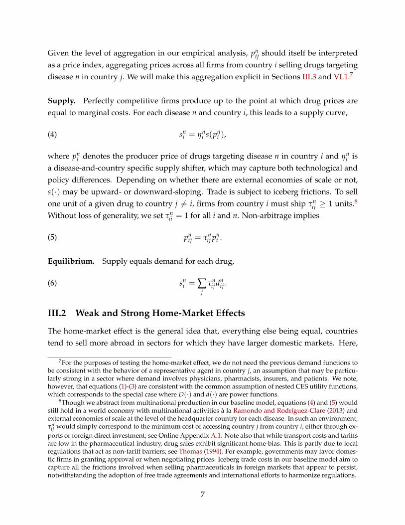
Figure 1: No Home-Market Effect

way to identify departures from the predictions of neoclassical trade models. The strongtest merely puts tighter bounds on the magnitude of these departures, if any.

Economic Interpretation. The economic forces that give rise to weak and strong home-market effects are best illustrated in a world economy comprising a large number of smallopen economies in the sense that each country is too small to affect the price of foreignvarieties, but large enough to affect the price of its own varieties, as in Gali and Monacelli(2005).11 In this case, the two elasticities, βX and βM, simplify into

βX =λ(1− εx)

εs + εw ,(10)

βM = 1 +λ2(1− εd)(εx − εD)

(1− λεd − (1− λ)εx)(εs + εw),(11)

where λ > 0 is the share of expenditure, as well as revenue, on domestic drugs in thesymmetric equilibrium; εd > 0 and εx > 0 are the lower-level elasticities of demandfor domestic and foreign varieties, respectively; εD > 0 is the upper-level elasticity ofdemand; εw ≡ λεd + (1− λ)εx − λ2(1− εd)(εd − εD)/(1− λεd − (1− λ)εx) > 0 is theelasticity of world demand; and εs is the elasticity of supply, which may be positive ornegative, depending on whether there are economies of scale.

Suppose that εx > 1 so that countries with lower prices tend to have higher marketshares abroad, which will be the empirically relevant case. Then, according to equation

11Formally, we obtain the small open economy limit by taking the number of countries in the worldeconomy to infinity and adjusting trade costs, τ, to leave the expenditure share on a country’s own good,λ, at a constant and strictly positive level.

10

q

p

s

d

(a) Price and Quantity

q

MX

(b) Exports and Imports

Figure 2: Weak Home-Market Effect

(10), there can only be a weak home-market effect in the presence of economies of scale,

εs < −εw < 0.

In a neoclassical environment, an increase in domestic demand across sectors, i.e. a pos-itive shift in θ, raises world demand, d, and in turn, producer prices, p, as depicted inFigure 1a. If the price elasticity of exports, εx, is strictly greater than one, this necessarilylowers the value of exports, X, as depicted in Figure 1b. By lowering the price of goodswith larger domestic markets, economies of scale can instead create a positive relationshipbetween exports and domestic demand, as described in Figures 2a and 2b.12

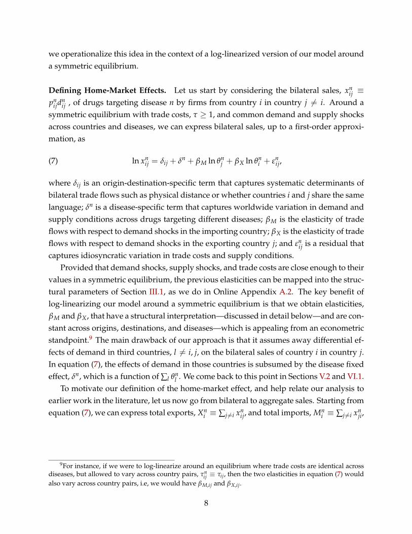
Suppose, in addition, that εd > 1 and εx ≥ εD. The second inequality is anothermild restriction that requires, for example, French and American drugs targeting cardio-vascular diseases to be closer substitutes than drugs targeting cardiovascular and skindiseases. Under this restriction, equations (10) and (11) imply that a strong home-marketeffect arises if economies of scale are strong enough to dominate the direct effect of do-mestic demand on imports, namely if

(12) − εw − λ[εx − 1 + (λ(1− εd)(εx − εD))/(1− λεd − (1− λ)εx)] < εs < −εw.

This situation is depicted in Figure 3.

12Even under the assumption that εx > 1, economies of scale are necessary, but not sufficient, for a weakhome-market effect to arise. Namely, if economies of scale are so strong that the equilibrium is Marshallianunstable, with supply curves steeper than demand curves, −εw < εs < 0, then drugs with larger demandhave higher prices, which leads to βX < 0, like in a neoclassical environment.

11

q

p

sd

(a) Price and Quantity

q

MX

(b) Exports and imports

Figure 3: Strong Home-Market Effect

III.3 Beyond Perfect Competition

We have conducted our theoretical analysis in a stylized model with perfect competition.The goal of this subsection is to establish the broader applicability of our empirical strat-egy. To do so, we provide four examples that illustrate how more complex economic en-vironments may nevertheless generate equilibrium conditions similar to those presentedin Section III.1, and, in turn, why our simple test and its economic interpretation maycarry over to these environments.

Our first example considers a monopolistically competitive model similar to the onestudied in Krugman’s (1980) original work, in which increasing returns at the sector levelreflect consumers’ love for variety and the positive relationship between entry and sectorsize. The other three examples, motivated by some key features of the global pharma-ceutical industry, introduce variable markups, endogenous innovation, and price regula-tions. For expositional purposes, we only sketch alternative models and summarize theirmain implications. Details can be found in Online Appendix A.3.

Monopolistic Competition. Consider an economy where what we have referred to as“country i’s variety” in Section III.1 is itself a composite of multiple differentiated vari-eties, each produced by monopolistically competitive firms, as in Krugman (1980).

Formally, suppose that country j’s consumption of drugs targeting disease n producedby a firm ω from country i is given by

(13) dnij(ω) = (pn

ij(ω)/pnij)−σdn

ij,

where pnij = (

∫(pn

ij(ω))1−σ)dω)1/(1−σ) is the CES price index and σ > 1 is the elasticity

12

of substitution between country i’s varieties. All other assumptions on the structure ofdemand are the same as in Section III.1. On the supply side, each firm must now pay anoverhead fixed cost, f n

i > 0, in order to produce. Once this fixed cost has been paid, firmshave a constant marginal cost, cn

i > 0. All firms maximize profits taking their residualdemand curves as given and enter up to the point where profits net of the overhead fixedcost are equal to zero.

At the industry-level, the previous assumptions lead to a supply curve similar to (4).Let us define Home’s aggregate supply of drug n as the following quantity index,

sni = (

∫(sn

i (ω))(σ−1)/σdω)σ/(σ−1),

where sni (ω) ≡ ∑j τn

ij dnij(ω) is the total quantity supplied by firm ω, regardless of whether

it is ultimately sold domestically or exported. Since demand is iso-elastic, monopolisti-cally competitive firms charge constant markups, µ ≡ σ/(σ − 1), over marginal costs.Together with free entry, this leads to

sni = (Nn

i )σ/(σ−1) f n

i /((µ− 1)cni ),

pni = (Nn

i )1/(1−σ)µcn

i .

where we let pni ≡ pn

ii denote the price index associated with country i’s varieties beforetrade costs have been incurred and we let Nn

i denote the measure of firms producingdrugs targeting disease n in country i. The two previous expressions provide a parametricrepresentation of the sector-level supply curve, with the number of firms Nn

i acting as aparameter. In this case, one can eliminate Nn

i to express the supply curve explicitly as

sni = ηn

i (pni )−σ,

with ηni ≡ f n

i (cni )

(σ−1)σσ(σ− 1)(1−σ). This is the counterpart of the supply equation (4).Finally, since firms charge the same markup µ in all markets, equation (5) must hold forthe price indices, pn

ij, of country i’s varieties of drug n in any importing country j.At this point, we have established that equations (1)-(5) continue to hold. By construc-

tion of our quantity index, equation (6) must hold as well, as shown in Online AppendixA.3. This implies that our test remains valid under monopolistic competition. The onlydistinction between the perfectly competitive model of Section III.1 and the present oneis that monopolistic competition requires sector-level supply curves to be downward-sloping, with an elasticity equal to the opposite of the elasticity of substitution between

13

domestic varieties,εs = −σ.

It is worth pointing out that the magnitude of the overhead fixed cost, f ni , is irrelevant for

the shape of s and, in turn, irrelevant for the existence of a home-market effect. Thoughpharmaceutical firms are well-known for having large expenditures on research and de-velopment relative to the cost of manufacturing a drug, it does not follow, according tothis monopolistically competitive model, that home-market effects should be particularlystrong in that industry. The economic variable of interest for home-market effects is themagnitude of industry-level returns to scale—determined by σ under monopolistic com-petition—not firm-level returns to scale.

Note also that in the special case considered by Krugman (1980)—with upper-levelCobb-Douglas utility, εD = 1, and lower-level CES utility, εx = εd = σ—the home-market effect is always strong for a small open economy. Indeed, under these parametricrestrictions, inequality (12) reduces to

−σ− λ(σ− 1) < −σ < −σ + λ2(σ− 1).

which must hold for any λ > 0 and σ > 1.

Variable Markups. Consider the same basic environment as in the previous example,but with a finite number of firms, Nn

i , that compete à la Bertrand in each sector. To sim-plify the analysis, we assume that all demand functions are iso-elastic, with D(x) =

d(x) = x−εd, and that there is an arbitrarily large number of diseases. Together these

assumptions imply that while markups may vary across origins and diseases, firms fromcountry i producing drugs that target disease n will charge the same markup across alldestinations. We will relax this restriction in our final example. The rest of the model isunchanged.

In equilibrium, firms still maximize their profits taking their residual demand curvesas given, albeit internalizing the effect of their decisions on the domestic price index asso-ciated with each disease. This leads to markups that now vary with the number of firmsNn

i . Formally, one can show that country i’s aggregate supply of drug n and its priceindex now satisfy

sni = (Nn

i )σ/(σ−1) f n

i /((µ(Nni )− 1)cn

i ),

pni = (Nn

i )1/(1−σ)µ(Nn

i )cni ,

14

with µ(Nni ) ≡

((1−1/Nni )σ+εd/Nn

i )

(1−1/Nni )σ+εd/Nn

i −1 denoting the firms’ markup under Bertrand competi-tion. Though one can no longer solve explicitly for sn

i as a function of pni , the two previ-

ous expressions still provide a parametric representation of the sector-level supply curve.Since equations (1), (2), and (5) remain unchanged, the existence of such a curve is all weneed to apply our test.

Locally, the price elasticity of supply is now given by

εs = −σ× (µ− 1)2 + (1− 1/σ)(d ln µ/d ln N)

(µ− 1)2(1− (σ− 1)(d ln µ/d ln N)).

Compared to monopolistic competition with constant markups, where d ln µ/d ln N = 0,the supply elasticity is lower in absolute value, |εs| < σ, whenever markups are decreas-ing with the number of firms, d ln µ/d ln N < 0. This is what happens for σ > εd. In thiscase, the larger aggregate output in an industry is, the more firms there are, the lower themarkups that they charge, and hence the lower the price that firms are willing to acceptto produce a given aggregate quantity. At the sector-level, pro-competitive effects act asan additional source of increasing returns.

Endogenous Innovation. Let us now consider an economy where countries only pro-duce a single variety of each drug, but unlike in our basic environment, this variety isproduced by a monopolist that can invest in R&D, as in Krugman (1984). We follow thesame strategy as in the previous example and assume that demand functions are iso-elastic, with D(x) = d(x) = x−εd

, and that there is an arbitrarily large number of drugsso that firms charge the same markup in all markets.

For each disease n, the monopolist in country i takes the residual demand curve ineach market as given when simultaneously choosing its prices, pn

ij, and its unit cost ofproduction, cn

i , in order to maximize its profits,

πni = ∑

j(pn

ij − τnij c

ni )d(pn

ij/Pnj )D(Pn

j /Pj)θnj Dj − ηn

i f (cni ),

where ηni f (cn

i ) denotes the amount of R&D required to have unit cost, cni , which we as-

sume to be strictly decreasing and convex.13 The first-order conditions associated with

13The monopolist could be a multinational firm. That is, fixed R&D costs—equal to ηni f (cn

i )—and vari-able production costs—proportional to τn

ij cni —could be incurred in different countries, with τn

ij cni the mini-

mum cost of accessing country j from country i through foreign direct investment, like in Online AppendixA.1. Bilir and Morales (2018) provide evidence of productivity gains from R&D benefiting affiliates in dif-ferent locations in the U.S. pharmaceutical industry.

15

this maximization problem imply the following version of the supply equation (4),

sni = −ηn

i f ′((εd − 1)pni /εd).

Under the assumption that f (·) is convex, drug-level supply curves are necessarily downward-sloping with local elasticity now given by

εs = d ln(− f ′)/d ln c.

The critical feature of the present model is that the marginal benefit of R&D is increasingwith total output, which creates a negative relationship between output and prices. On-line Appendix A.3 demonstrates that the same analysis extends to environments wherethe monopolist needs to pay a fixed cost in order to sell in each destination as well asin environments where the monopolist can use R&D to increase the quality of its drugsrather than to lower their costs.

Price Regulations. To conclude, we focus on an economy similar to the previous one,where monopolists are free to invest in R&D to lower their production costs, cn

i , but wenow let governments, rather than firms, set prices. Formally, we relax the non-arbitragecondition (5) and assume instead that

pnij = µn

ijτnij c

ni .

where the markup, µnij, is taken as an exogenous characteristic that reflects the bargaining

power of the government from country j vis-à-vis the firm from country i producingdrugs that target disease n. For the same reason as in the previous example, supplysatisfies

sni = −ηn

i f ′(cni ).

Except for equation (5), all other equations from Section III.1 still hold, with the conven-tion pn

i ≡ cni . As demonstrated in Online Appendix A.3, this implies that equation (7)

must hold as well, with the two elasticities, βX and βM, still determined by the elasticitiesof supply and demand. The key difference is that the exogenous markups, µn

ij, are nowpart of the error term in equation (7), a point to which we return in Section V.3.

Summary. The previous examples help clarify a number of points. First, there are manymarket structures, beyond Krugman’s (1980) monopolistically competitive environment,that can give rise to a home-market effect. Second, the existence of a home-market effect,

16

in each of these examples, is intimately related to the existence of increasing returns atthe sector-level, i.e., whether or not supply slopes down. Third, depending on the partic-ular market structure, the nature of sector-level economies of scale may be very different.In our final example, it depends on the elasticity of the marginal returns to R&D; previ-ously, it derived from Marshallian externalities, love of variety, or pro-competitive effects.Fourth, independently of the nature of economies of scale, our test of the home-marketeffect remains valid. This suggests that our test of the home-market effect can be appliedto many industries, including the global pharmaceutical industry. This is the empiricalapplication that we now turn to.

IV DATA

Our analysis of the home-market effect rests on the correlation between a country’s pat-tern of sales across drugs in the pharmaceutical sector and its pattern of exogenously-given demand across those drugs. We therefore draw on a linkage between two datasets:one that documents sales by country at the drug level, which we convert to a dataset ofbilateral sales as detailed below, and one that describes the demographically-driven bur-den of each disease in each country. In both cases we use data from one cross-section,from 2012, which suffices for testing the home-market effect since its prediction is cross-sectional in nature.

IV.1 Pharmaceutical Sales

In order to construct bilateral data on pharmaceutical sales, {xnij}, we draw on the IMS

MIDAS dataset produced by the firm IMS Health. IMS is a market research firm that sellsMIDAS and other data products to firms in the pharmaceutical and health care industries.By auditing retail pharmacies, hospitals, and other sales channels, the raw IMS MIDASdata record quarterly revenues and quantities by country at the “package” level, e.g. salesof a bottle of thirty 10mg tablets of the cholesterol-lowering drug Lipitor (atorvastatin).The data record unit sales and revenues (in local currency units), for both private andpublic purchasers.14

Our version of the IMS MIDAS dataset covers sales in 56 destination countries.15

14Online Appendix B.3 describes how pharmaceutical sales from the IMS MIDAS dataset compare tothose from two publicly available data sources: the OECD HealthStat database and the Medical Expendi-ture Panel Survey (MEPS).

15The most recent versions of the IMS MIDAS dataset cover more than 70 countries. Our 56 destinationcountries are Algeria, Argentina, Australia, Austria, Belgium, Brazil, Bulgaria, Canada, China (mainland),

17

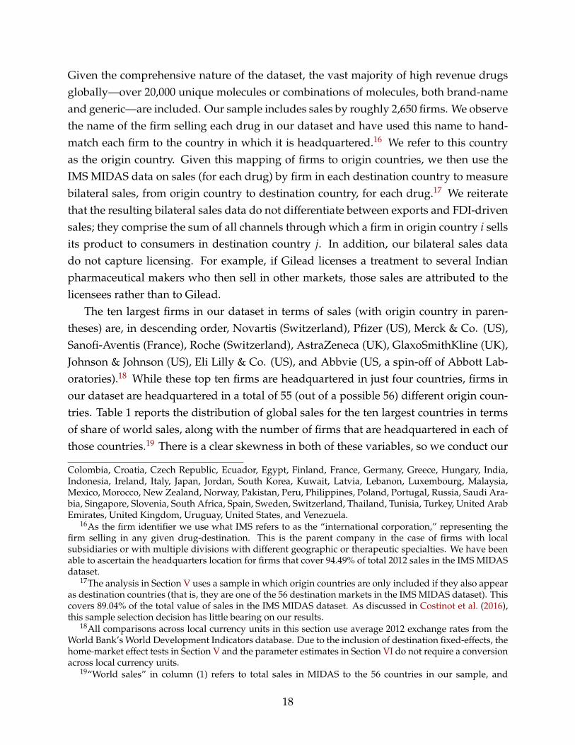
Given the comprehensive nature of the dataset, the vast majority of high revenue drugsglobally—over 20,000 unique molecules or combinations of molecules, both brand-nameand generic—are included. Our sample includes sales by roughly 2,650 firms. We observethe name of the firm selling each drug in our dataset and have used this name to hand-match each firm to the country in which it is headquartered.16 We refer to this countryas the origin country. Given this mapping of firms to origin countries, we then use theIMS MIDAS data on sales (for each drug) by firm in each destination country to measurebilateral sales, from origin country to destination country, for each drug.17 We reiteratethat the resulting bilateral sales data do not differentiate between exports and FDI-drivensales; they comprise the sum of all channels through which a firm in origin country i sellsits product to consumers in destination country j. In addition, our bilateral sales datado not capture licensing. For example, if Gilead licenses a treatment to several Indianpharmaceutical makers who then sell in other markets, those sales are attributed to thelicensees rather than to Gilead.

The ten largest firms in our dataset in terms of sales (with origin country in paren-theses) are, in descending order, Novartis (Switzerland), Pfizer (US), Merck & Co. (US),Sanofi-Aventis (France), Roche (Switzerland), AstraZeneca (UK), GlaxoSmithKline (UK),Johnson & Johnson (US), Eli Lilly & Co. (US), and Abbvie (US, a spin-off of Abbott Lab-oratories).18 While these top ten firms are headquartered in just four countries, firms inour dataset are headquartered in a total of 55 (out of a possible 56) different origin coun-tries. Table 1 reports the distribution of global sales for the ten largest countries in termsof share of world sales, along with the number of firms that are headquartered in each ofthose countries.19 There is a clear skewness in both of these variables, so we conduct our

Colombia, Croatia, Czech Republic, Ecuador, Egypt, Finland, France, Germany, Greece, Hungary, India,Indonesia, Ireland, Italy, Japan, Jordan, South Korea, Kuwait, Latvia, Lebanon, Luxembourg, Malaysia,Mexico, Morocco, New Zealand, Norway, Pakistan, Peru, Philippines, Poland, Portugal, Russia, Saudi Ara-bia, Singapore, Slovenia, South Africa, Spain, Sweden, Switzerland, Thailand, Tunisia, Turkey, United ArabEmirates, United Kingdom, Uruguay, United States, and Venezuela.

16As the firm identifier we use what IMS refers to as the “international corporation,” representing thefirm selling in any given drug-destination. This is the parent company in the case of firms with localsubsidiaries or with multiple divisions with different geographic or therapeutic specialties. We have beenable to ascertain the headquarters location for firms that cover 94.49% of total 2012 sales in the IMS MIDASdataset.

17The analysis in Section V uses a sample in which origin countries are only included if they also appearas destination countries (that is, they are one of the 56 destination markets in the IMS MIDAS dataset). Thiscovers 89.04% of the total value of sales in the IMS MIDAS dataset. As discussed in Costinot et al. (2016),this sample selection decision has little bearing on our results.

18All comparisons across local currency units in this section use average 2012 exchange rates from theWorld Bank’s World Development Indicators database. Due to the inclusion of destination fixed-effects, thehome-market effect tests in Section V and the parameter estimates in Section VI do not require a conversionacross local currency units.

19“World sales” in column (1) refers to total sales in MIDAS to the 56 countries in our sample, and

18

tests of the home-market effect in a wide range of subsamples designed to explore poten-tial heterogeneity across large and small countries, as well as countries (such as India andChina) where the large number of headquartered firms reflects a relatively large share ofgeneric drug producers.

IMS uses a standard industry classification known as ATC codes, from the AnatomicalTherapeutic Classification System, to classify molecules into approximately 600 differenttherapeutic classes based on the main disease the drug is designed to treat.20 To link backto the example in our introduction, the ATC code “A2B2” corresponds to “acid pumpinhibitors.”

The resulting dataset can be reshaped to describe, within each therapeutic class, thebilateral sales between any origin country and any of 56 destination countries in 2012.

IV.2 Disease Burden

We isolate a plausibly exogenous source of demand-side variation for each drug, in eachcountry, by isolating the apparent extent to which drugs have a demographic bias in theirrelevance, as well as the extent to which countries differ in the demographic compositionof their populations. This is the spatial analog of the identification strategy in Acemogluand Linn (2004), who use changes in the age distribution of the United States over timeto estimate the relationship between market size and innovation in the pharmaceuticalindustry.

To construct this demand shifter, we draw on two datasets. The first, the WorldHealth Organization (WHO)’s Global Burden of Disease (GBD) dataset, measures theburden of each disease, based on WHO-assigned disease codes,21 in each country andyear (where, again, we focus on 2012). Although there may be local variation in the col-lection of vital statistics that underpin these measures, the WHO ensures that these dataare valid for cross-country and cross-disease comparisons. Importantly, these country-year-disease measures of burden are further broken down into six different demographic

analogously for “world expenditures” in column (2). The number of firms in column (3) refers to firmsmaking strictly positive sales in 2012 to at least one of the 56 countries in our sample.

20IMS’s ATC classification is maintained by the European Pharmaceutical Market Research Association,and should not be confused with the World Health Organization’s Anatomical Therapeutic Chemical clas-sification.

21The underlying WHO data is provided in a tree structure that includes both “aggregate” codes and“root” codes. For example, that file records disease burden data for “Infectious and parasitic diseases,”“Childhood cluster diseases” and “Pertussis.” In the tree structure of the file, “pertussis” is containedwithin “childhood cluster diseases” which in turn are contained in “infectious and parasitic diseases.”“Pertussis” has no further subcategories (which we refer to as an example of a “root” code), whereas theother two are aggregates of other subcategories. We focus our analysis on the “root” codes, so as to avoiddouble-counting.

19

groups: three age groups (0-14, 15-59 and 60+) for each gender. The provided diseaseburden measure on which we draw is the number of lost disability adjusted life-years(DALYs)—combining data on both the mortality and morbidity caused by each disease.

We have hand-coded a many-to-one linkage from each of the 600 therapeutic classes(ATC codes) in IMS MIDAS to its corresponding WHO disease code. For example, theATC code “A2B2” for “acid pump inhibitors” is linked to the WHO code for “peptic ulcerdisease.” Using the most disaggregated WHO disease codes for the year 2012 for whichwe have disease burden data and a corresponding ATC code in the IMS sales data, wematch 60 of the GBD 2012 codes to the ATC codes in the IMS.22 The full crosswalk canbe found in Online Appendix B.4. In practice, two of the 60 WHO disease codes haveno recorded global sales in our sample in 2012, implying that our actual analysis sampleincludes 58 diseases.23 Each of the WHO disease codes is the empirical counterpart of adisease n in the model of Section III.

Table 2 describes the top 10 diseases (broken down by WHO codes) in terms of globalsales of their corresponding drugs in the IMS MIDAS dataset. For each disease, thereare many origin countries participating in the sale of drugs treating that disease. As il-lustrated in the last column, the typical destination country in our data is served by anextremely unconcentrated set of firms, even within each disease class.

The second input into the construction of our demand shifter is the population of eachcountry in each of the six demographic groups in 2012. We obtain this data from the USCensus Bureau’s International Database.

Using the data described above, we exploit the twin facts that disease burdens varyby demographic groups, and that countries vary in their demographic composition, toconstruct a “predicted disease burden”, for disease n in country i in year 2012 as:

(14) (PDB)ni = ∑

a,g

[populationiag ×

(∑k 6=i disease burdenn

kag

∑k 6=i populationkag

)].

The ratio ∑k 6=i disease burdennkag

∑k 6=i populationkagmeasures the average disease burden per capita from dis-

ease n for gender g and age group a in 2012, calculated excluding the country of interest(that is, summing over all countries k except for country i).24 This ratio is then weighted

22One GBD code, U047 for “Abortion,” is missing disease burden data; we impute the disease burden tobe zero in this case.

23Around 89% of our ATC4 codes were linked to WHO GBD codes. The main reason for non-matches isthat certain ATC4 codes are too broad to be matched to a single GBD disease code.

24The fact that firms from country i are better at treating disease n may cause a lower burden for that

20

Japan

Bulgaria

Pakistan

United Arab Emirates

.7.8

.91

Shar

e of

cou

ntry

pop

ulat

ion

with

age

bel

ow 6

0

Countries

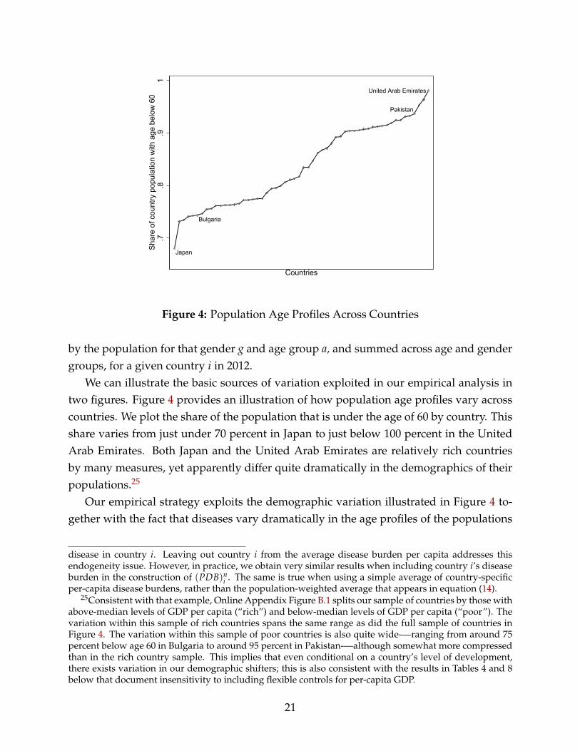
Figure 4: Population Age Profiles Across Countries

by the population for that gender g and age group a, and summed across age and gendergroups, for a given country i in 2012.

We can illustrate the basic sources of variation exploited in our empirical analysis intwo figures. Figure 4 provides an illustration of how population age profiles vary acrosscountries. We plot the share of the population that is under the age of 60 by country. Thisshare varies from just under 70 percent in Japan to just below 100 percent in the UnitedArab Emirates. Both Japan and the United Arab Emirates are relatively rich countriesby many measures, yet apparently differ quite dramatically in the demographics of theirpopulations.25

Our empirical strategy exploits the demographic variation illustrated in Figure 4 to-gether with the fact that diseases vary dramatically in the age profiles of the populations

disease in country i. Leaving out country i from the average disease burden per capita addresses thisendogeneity issue. However, in practice, we obtain very similar results when including country i’s diseaseburden in the construction of (PDB)n

i . The same is true when using a simple average of country-specificper-capita disease burdens, rather than the population-weighted average that appears in equation (14).

25Consistent with that example, Online Appendix Figure B.1 splits our sample of countries by those withabove-median levels of GDP per capita (“rich”) and below-median levels of GDP per capita (“poor”). Thevariation within this sample of rich countries spans the same range as did the full sample of countries inFigure 4. The variation within this sample of poor countries is also quite wide-—ranging from around 75percent below age 60 in Bulgaria to around 95 percent in Pakistan-—although somewhat more compressedthan in the rich country sample. This implies that even conditional on a country’s level of development,there exists variation in our demographic shifters; this is also consistent with the results in Tables 4 and 8below that document insensitivity to including flexible controls for per-capita GDP.

21

U087

U078

U089

U086

U012

0.2

.4.6

.81

Shar

e of

glo

bal d

isea

se b

urde

nbo

rne

by p

opul

atio

n be

low

age

60

GBD codes

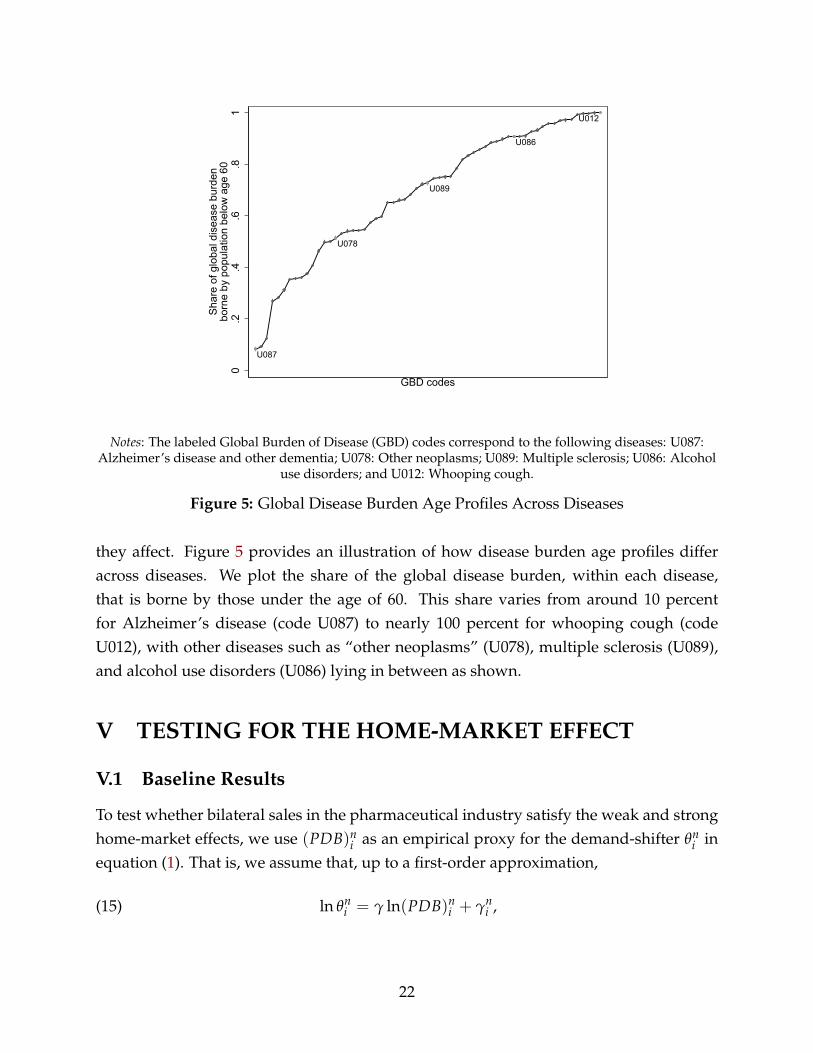
Notes: The labeled Global Burden of Disease (GBD) codes correspond to the following diseases: U087:Alzheimer’s disease and other dementia; U078: Other neoplasms; U089: Multiple sclerosis; U086: Alcohol

use disorders; and U012: Whooping cough.

Figure 5: Global Disease Burden Age Profiles Across Diseases

they affect. Figure 5 provides an illustration of how disease burden age profiles differacross diseases. We plot the share of the global disease burden, within each disease,that is borne by those under the age of 60. This share varies from around 10 percentfor Alzheimer’s disease (code U087) to nearly 100 percent for whooping cough (codeU012), with other diseases such as “other neoplasms” (U078), multiple sclerosis (U089),and alcohol use disorders (U086) lying in between as shown.

V TESTING FOR THE HOME-MARKET EFFECT

V.1 Baseline Results

To test whether bilateral sales in the pharmaceutical industry satisfy the weak and stronghome-market effects, we use (PDB)n

i as an empirical proxy for the demand-shifter θni in

equation (1). That is, we assume that, up to a first-order approximation,

(15) ln θni = γ ln(PDB)n

i + γni ,

22

where γ is strictly positive and γni captures other determinants of the demand-shifter θn

ifor drugs targeting disease n in country i that are uncorrelated with (PDB)n

i . Table B.1in Online Appendix B establishes that the variable (PDB)n

i is a strong predictor of theactual burden that any country i is likely to suffer from for disease n. That is, the simpledemographic predictor of disease burden in equation (14) is a useful empirical proxy forθn

i , despite the myriad other reasons for countries to differ in their demand for drugstargeting any particular disease.26 Our results in Table 3 below demonstrate that thisproxy is also a strong predictor of expenditure.

In order to estimate βX and βM, one could use either the cross-sectional variation in bi-lateral sales, i.e. equation (7), or the cross-sectional variation in total exports and imports,i.e. equations (8) and (9). Like in recent empirical tests of other sources of comparativeadvantage (e.g. Chor, 2010 and Costinot et al., 2012), we prefer to use the former. Theadvantage of this strategy is that it lets us control for variation in trading frictions anddemand across destination countries when estimating the impact of a given source ofcomparative advantage across origin countries, here their own demand. In contrast, evenaround a symmetric equilibrium, total exports, Xn

i , do not only depend on a country’sown demand, but also on its access to foreign buyers, ln(∑j 6=i(θ

nj )

βM exp(δij + εnij)). If

demand shocks are spatially correlated across countries, estimates of βX obtained fromequation (8) would therefore be biased. Under the same assumptions, estimates of βX

obtained from equation (7) are not.Combining equations (7) and (15), we have the following baseline estimating equation,

(16) ln xnij = δij + δn + β̃M ln(PDB)n

j + β̃X ln(PDB)ni + ε̃n

ij,

with β̃M ≡ γβM, β̃X ≡ γβX, with δij and δn represented by origin-destination anddisease fixed-effects respectively, and with the error term given by ε̃n

ij ≡ εnij + βXγn

i +

βMγnj . Under the assumption that γ > 0, a positive test of the weak home-market ef-

fect therefore corresponds to β̃X > 0, whereas a positive test of the strong home-marketeffect corresponds to β̃X > β̃M. And under the assumption that ln(PDB)n

i is a puredemand-shifter—such that it is uncorrelated with the supply shifter ηn

i and hence theerror ε̃n

ij—both β̃X and β̃M can be estimated using OLS, as we do below.27

26The two-stage least squares specification that we would ideally estimate would instrument for ourdemand-shifter θn

i with our predicted disease burden measure. However, in practice θni is unobserved.

In Online Appendix Table B.1, we show that our predicted disease burden measure is correlated with theactual disease burden at the country-disease level. However, actual disease burden is not equivalent to θn

i ,so the first stage “scaling” provided by the estimates in Online Appendix Table B.1 is not the conceptuallycorrect scaling from the perspective of estimating a two-stage least squares regression.

27We stress at this point that the coefficient estimates of β̃M and β̃X are valid for testing the weak and

23

Several details of the estimation procedure used in this section are worth mentioning.First, we estimate equation (16) on a sample of ij observations for which i 6= j, in line withthe derivation of equation (7). This ensures that the trivial correlation between home’sdemand shifter and sales from home to itself does not enter the analysis (however, as weshow in Table 7, incorporating this variation does little to change our findings). Second, inour baseline estimates we drop observations for which xn

ij = 0, but we return this aspect ofthe variation in Table 8. And finally, because the predicted disease burden regressors varyat the origin and destination levels (but not at the bilateral level) we provide standarderrors that are two-way clustered at both the origin and destination levels throughout.

Table 3 presents OLS estimates of equation (16). We begin in column (1) with a spec-ification designed to estimate β̃M as accurately as possible. To do so we control for anorigin-disease fixed-effect (rather than including the origin country’s predicted diseaseburden). While the estimate of β̃M > 0 seen there should not be surprising—a demandshifter in the destination country is positively correlated with greater purchases by thatdestination—this can be thought of as a check on the validity and power of demographicvariation for predicting drug expenditure. Column (2) proceeds with an analogous spec-ification designed to estimate β̃X alone, as accurately as possible, while controlling for adestination-disease fixed-effect. The estimated value of β̃X is clearly positive and statis-tically significant. This result (and the accompanying p-value for the one-sided t-test ofβ̃X ≤ 0) provides a resounding rejection of the absence of a weak home-market effect.

Finally, column (3) estimates β̃M and β̃X simultaneously in the true spirit of equation(7). This is our preferred specification. We first note that the estimates of β̃M and β̃X incolumn (3) are very similar to those in columns (1) and (2), so evidence for the weak home-market effect remains firm. And the p-value on the F-test for β̃X ≤ β̃M is 0.018, implyingthat the absence of a strong home-market effect can be rejected at the five percent level.28

That is, it seems likely that the strong home-market effect is at work in the pharmaceuticalsector.29

strong home-market effects, and have a structural interpretation as discussed in Section III.2. But they arenot sufficient for conducting comparative statics analyses of the effects of PDB on bilateral sales becauseof the fact that the disease fixed-effect δn is also a function of each country’s PDB, as established in OnlineAppendix A.2. The same observation applies to other comparative static exercises, like the introduction ofimport tariffs in the pharmaceutical sector.

28With standard errors that are clustered three-way at the origin country, destination country and dis-ease levels (following Cameron et al., 2011) the standard errors on β̃M and β̃X are (0.218) and (0.232),respectively. The p-values for the tests of β̃X ≤ 0 and β̃X ≤ β̃M are 0.000 and 0.115, respectively.

29This is equally true when we estimate equation (16) on IMS MIDAS data from 2004, the earliest yearfor which comparable data is available. In that case the estimates (and standard errors) of β̃M and β̃X are0.582 (0.076) and 0.910 (0.166), respectively.

24

V.2 Why Does Home Demand Matter?

The results above demonstrate a reduced-form relationship between a country’s homedemand for a drug category and foreign sales. But why does home demand matter inthis way? Section III described a range of theoretical settings in which the industry-levelsupply curve is downward-sloping and it is this feature, and only this feature, that ex-plains why home demand matters for export success. We now discuss two alternativeexplanations that could, in principle, provide equally plausible answers to the questionof why home demand matters.

Alternative I: Home demand is positively correlated with supply-side considerationsdriving the pattern of international specialization. As discussed above, equation (16)describes the pattern of equilibrium drug expenditure around the world due to funda-mental demand-side (PDBn

i and PDBnj ) and supply-side (ηn

i , a component of ε̃nij) consid-

erations. If PDBni and ε̃n

ij were positively correlated, our OLS estimates of β̃X would bebiased upwards, potentially generating the appearance of a home-market effect, whenother forces are at play.

One possible reason for such a positive correlation is that a common factor explainsboth variables. For example, in Vernon’s (1966) theory of the product cycle, drugs wouldinitially be produced in high-income countries and eventually be produced in poorercountries. Since one might expect the demographic ingredients of PDB to be equallydistinct across high- and low-income countries, it is possible that per-capita GDP is acommon factor that affects both demand and supply in a manner that would confoundestimation of β̃X.

To assess this possibility, column (2) of Table 4 tests for the two home-market effects ina specification that also simultaneously controls for per-capita GDP as a source of compar-ative advantage, that is, for the interaction between the origin country’s per-capita GDPand disease fixed-effects, as well as for the analogous variable on the destination countryside. Compared to our baseline estimates in Table 3, reported in column (1) for the sakeof comparison, the null of no weak home-market effect can still be rejected at standardconfidence levels, while this is no longer true for the null of strong home-market effect.Reassuringly, however, the point estimates of β̃M and β̃X have not changed much in com-parison with the estimates in column (1). This suggests that although there may be somesystematic tendency for poor countries to produce certain drugs—in line, for instance,with Vernon (1966)—these drugs do not happen to treat the diseases associated with poorcountry demographics.

Symmetrically, column (3) reports a specification that controls for interactions be-

25

tween country (origin and destination) fixed-effects and a measure of disease intensity(the decile in which a disease falls in the worldwide distribution, based on its diseaseburden). This allows some countries to have a comparative advantage in the most severediseases, due to some unobserved country-specific characteristic that may be differentfrom per-capita GDP. Again, the stability of the key coefficients, β̃M and β̃X, implies thatthey are being identified from the intended demographic-related component of diseaseburden, rather than some other pattern related to disease burden more generally. In con-trast to column (2), the p-value on the F-test for β̃X ≤ β̃M also implies that the absenceof a strong home-market effect can be rejected at the one percent level. In short, Table4 implies that potential common contributors to both demand-side and supply-side de-terminants of international specialization based on countries’ income levels or diseases’overall severity may exist, but not in a way that appreciably affects our estimates.

A second possible source of correlation between demand (PDBni ) and supply (ε̃n

ij)could be more direct. For example, government funding of medical research may re-flect, at least in part, the needs of the local population; see Lichtenberg (2001). Similarly,clinical trials may be cheaper to conduct in countries with a large pool of potential sub-jects. If so, one would expect the supply shifter ηn

i , and hence the residual, ε̃nij, to be an

increasing function of ln(PDB)ni ,

(17) ε̃nij = ψ ln(PDB)n

i + νnij,

with ψ > 0 and νnij uncorrelated with ln(PDB)n

i . In such cases, it is important to note thatour empirical test of the home-market would remain valid in the sense that we could stillestimate (16) using OLS to test whether an increase in domestic demand, as proxied byln(PDB)n

i , tends to raise exports. The structural interpretation of the estimated elastici-ties, however, would change. For instance, in the case of a small open economy discussedin Section III.2, the OLS estimate of the elasticity of ln xn

ij with respect to ln(PDB)ni would

now be equal to the sum of γλ(1− εx)/(εs + εw) and ψ.To separate out the economic mechanism described in Section III from the potential

confounders discussed here, the most direct empirical strategy would be to control forthese supply-side determinants, the same way we have controlled for per-capita GDPand disease severity in Table 4. Unfortunately, we lack systematic information about sub-sidies and the cost of clinical trials at the disease-country level. What is available is dataon subsidies from the US National Institutes of Health (NIH). Using data from Azoulay etal. (2018) on subsidies paid from each NIH sub-institute, we derive a measure of how ex-

26

posed each disease group in our data is to NIH subsidies.30 Column (2) of Table 5 reportsthe counterpart of our baseline results for diseases aggregated up to this NIH institutelevel, with the United States as the only origin country. Since this new specification lacksthe analog of a disease fixed-effect that can only be included in a sample which includesmultiple origin countries, the estimates cannot be compared directly with those from ourbaseline specification (again, included in column (1) for reference). It is nevertheless note-worthy that the results resoundingly reject the absence of a strong home-market effect onthis US sample. More importantly, column (3) demonstrates that controlling for (log) NIHspending has little impact on our point estimates.31

As an alternative, we now return to our baseline specification, but restrict the sampleof drugs and countries to those for which we expect government subsidies and the costsof clinical trials to be minimal. Column (4) in Table 5 looks only at drug sales for genericdrugs (where the original molecule is no longer subject to intellectual property protectionand hence is free to be produced by any firm), dropping sales of branded drugs (on whichintellectual property rights still apply). The fact that we continue to reject the lack ofa weak home-market effect in column (4) suggests that our baseline estimates are notcaused entirely by a correlation between demographic-driven demand and demographic-driven supply (i.e. ψ > 0). It is notable, however, that within this generics sub-sector ofthe pharmaceutical industry, it appears that economies of scale are not strong enoughto generate the strong home-market effect. As an alternative approach, we can focus oncountries which we expect are more likely to solely produce generics (namely, poorercountries): as column (5) demonstrates, we continue to reject the lack of a weak home-market effect when using a sample that excludes the richest third of origin countries (interms of GDP per capita).

Alternative II: Home demand is positively correlated with demand in neighboringcountries. A different explanation for the importance of home demand documented inTable 3 comes from the potential for a country’s own home demand to be correlated withdemand conditions abroad in ways that are not accounted for in equation (16). Arounda symmetric equilibrium, we have shown that our test of the home-market effect does

30The Azoulay et al. (2018) data on NIH subsidies is available from 1980-2005. To remain consistent withthe cross-sectional nature of our empirical exercise, we only work with the latest year, 2005. We mergethe 17 NIH sub-institutes into our 58 disease codes by hand. For three disease codes (abortion, maternalconditions, and poisoning) we deemed the merge indeterminate and drop those disease codes from oursubsequent analysis. Six NIH sub-institutes (e.g. National Human Genome Research Institute) were alsounmatched, leaving us with 11 aggregated disease categories that cover 55 of our original disease codes.

31The coefficient (and standard error) on the NIH log spending variable in this specification is 0.124(0.103).

27

not require any restriction on the spatial correlation of demand shocks across countries.As already mentioned in Section III.2, demand in countries different from the origin andthe destination should simply be absorbed by a disease fixed-effect. In general, however,even if all the assumptions of Section III.1 are satisfied, a country’s pattern of specializa-tion may not only reflect the variation in its own demand, but also the variation in itsneighbors’ demand, through the direct effect on the quantities that they consume and theindirect effect on the price of the drugs that they produce, the variation in the neighborsof its neighbors’ demand, etc.

Theoretically, it is unclear under which conditions, if any, the previous considerationsshould lead to a generalization of equation (7) in which the two elasticities, βM and βX, re-main constant and a country’s “home-market” becomes the distance-weighted sum of itsneighbors’ demand or some more general function of demand around the world. For thisreason, we prefer to stick to the issue of whether a country’s own demand, i.e., literallyits home market, provides a source of comparative advantage and treat the variation indemand from neighboring countries as another potential source of omitted variable bias.Empirically, the question of interest is whether there is evidence in the data for strongmultilateral effects, beyond those already absorbed by our disease fixed-effect.

Table 6 explores this issue. Again, column (1) repeats our baseline estimate for the pur-pose of comparison. Columns (2) and (3) show that restricting sales to a “donut” of desti-nation countries, either located at more than 1,000 km or 2,000 km from the home market,has little effect on the economic magnitude of our estimates, although the statistical sig-nificance of the strong home market effect weakens in the 2,000 km specification.32 Thesame is true in column (4) when we control for the average disease burdens in all othercountries, weighted by their distance to the origin and destination country; formally, weestimate a version of equation (16) that also includes the regressors ∑k 6=i ln PDBn

k · dist−1ik

and ∑k 6=j ln PDBnk · dist−1

kj . Put together, these results imply that multilateral considera-tions, at least according to the proxies used here, do not appear to be a source of quantita-tively meaningful departures from our log-linearization around a symmetric equilibrium.

In this final regression, we note that the coefficients (and standard errors) on ∑k 6=j ln PDBnk ·

dist−1kj and ∑k 6=i ln PDBn

k · dist−1ik are 0.591 (1.576) and −0.772 (3.623) , respectively. The

fact that the latter coefficient (while imprecisely estimated) is negative is consistent withthe possibility that neighboring countries may benefit disproportionately more from anincrease in their own demand, thereby reducing the price of their drugs relative to coun-

32Data on bilateral country pair distance (calculated from population-weighted averages of bilateralmajor city pair distances) are from the CEPII Gravity dataset; see Head and Mayer (2010).

28

try i’s and, in turn, lowering the residual demand faced by country i.33

V.3 Further Sensitivity Checks

We now assess the robustness of our results to a miscellany of alternative specificationsand modeling assumptions.

Pricing-to-Market. One potential concern is that firms in our setting can engage in sub-stantial pricing-to-market, due to prohibitions on international resale, and hence that thenon-arbitrage equation (5) may not apply. Although we have already demonstrated inSection III.3 that our empirical test may remain theoretically valid in the absence of thisequation, we now revisit this issue empirically. Specifically, in Table 7 column (2) we limitthe sample of destination markets to those within the EU, a free trade area where paralleltrade makes pricing-to-market difficult to sustain; see Scott Morton and Kyle (2012) forfurther discussion.34 If one thought that pricing-to-market had a significant effect on therelationship between drug sales and home demand, then one would expect different elas-ticities, β̃X and β̃M, in the EU sample. For instance, if governments were able to negotiatelower drug prices for diseases with greater burdens in their populations, there would bea negative correlation between ε̃n

ij and ln(PDB)nj in equation (16), driven by the lower

markup µjij in destinations with high PDBn

j . This would lead to larger estimates of β̃M inthose countries compared to those within the EU, for which markups are more likely tobe constant across destinations. While the effect of destination PDB for the EU sampleis imprecisely estimated (so it remains within the 95 percent confidence interval of ourbaseline estimate, repeated again in column (1) for comparison), the lower point estimateof β̃M gives some support to that view.35 For our purposes, the main take-away from this

33This finding is reminiscent of “agglomeration shadows” (e.g. Arthur, 1990; Matsuyama, 2017). Theidea is that countries surrounded by larger neighbors may face lower demand for their products, in spiteof the fact that having larger neighbors tends to mechanically raise demand. We note, however, that anegative coefficient on ∑k 6=i ln PDBn

k · dist−1ik does not imply that the total effect of larger neighbors is to

reduce demand. In our regression, we already control for the size of demand PDBnj at any given destination

j. Hence, the mechanical effect of demand in larger neighbors is not being picked up by ∑k 6=i ln PDBnk ·

dist−1ik . A negative coefficient merely suggests that countries surrounded by larger neighbors face tougher

competition in otherwise bigger markets.34More precisely, we focus here on the set of countries in our sample that were members of the European

Single Market as of 2012, which includes Norway and Switzerland as well as EU members.35In addition, this result implies that predicted disease burdens are not a strong predictor of conditional

demand among these destinations. However, in an analogous specification that instead restricts attentionto EU origin countries only we estimate (with standard errors in parentheses) β̃M = 0.366 (0.123) and β̃X =0.875 (0.715). One possible reason for the importance of PDB in predicting exporting success, relative todemand, among this set of countries is the fact that exporting success is likely to reflect lagged demand and

29

sensitivity check is that the estimated value of β̃X is again quite similar to that in previousspecifications. Hence, the weak home-market effect remains operational within the EUsample.

Foreign Direct Investment. As discussed above, a limitation of the MIDAS pharmaceu-tical dataset used throughout our empirical analysis is that it does not provide informa-tion about where a firm’s final product is made. We only know where a firm sells itsproducts and where it is headquartered. Accordingly, the economies of scale underpin-ning the home-market effect that we have documented earlier could have multiple roots.For instance, it could be the case that there are local economies of scale at the produc-tion site and the headquarter location is a good proxy for the location of production sites(which would be the case if multinational production is not widespread); or there couldbe local economies of scale at the R&D site and the headquarter location is a good proxyfor the location of R&D sites; or there may be economies of scale across affiliates from thesame firm in a given headquarter country.

We are unaware of any dataset that could be used to disaggregate total sales xnij into

FDI and export sales at the country pair-disease level. But publicly available (OECD) dataon international trade flows record the value of exports by country pair for the pharma-ceutical sector as a whole. By comparing total OECD exports to total MIDAS foreign sales,we can therefore obtain an estimate of the importance of trade relative to FDI for a givenorigin country.36 Using such information, column (3) estimates our baseline specificationon the subset of country pairs for which the ratio of total OECD exports to total MIDASforeign sales is above the median. If economies of scale were primarily operating at thelevel of the production sites, we would expect a stronger home-market effect in this sub-sample since foreign sales are more likely to occur through exports from a single origincountry. The stability of our estimated coefficients to this subsample is suggestive of thenotion that, in our context, this type of economies of scale is unlikely to be prevalent.

intra-EU pharmaceutical resale is a relatively recent phenomenon. For example, according to the EuropeanMedicines Agency’s Parallel Distributor Register, 20 licenses had been granted for the resale of 20 differentdrugs in 2000, but these figures had risen to 1,799 licenses for 257 drugs as of 2012.

36We draw on OECD BTDIxE data for 2012, corresponding to the industry activity category “Basic phar-maceutical products and pharmaceutical preparations” and the end use category “Total trade in goods”,as reported by the importing country. It should be clear that beyond the presence of bilateral FDI, whichis what we are interested in, there are multiple reasons to expect imperfect alignment of MIDAS bilateral(all-disease) foreign sales and OECD bilateral pharmaceutical export data. These include: exports occur-ring as platform FDI, intermediate inputs, or uncorrected re-exporting; differing pricing concepts (retail vs.border prices); differing sets of products included in pharmaceuticals (notably the OECD data’s inclusion ofveterinary drugs); and data reporting issues (e.g. misreporting in either dataset, miscoding of headquarterlocations, timing of exporting vs. sales within the calendar year, and confidentiality restrictions in OECDdata). Reassuringly, however, the correlation between the two sources is 0.595 (or 0.628 in logs).

30

Endogenous Demographics. Another possibility is that our baseline results are biaseddownwards due to the fact that a country’s demographic composition could itself beshaped by its disease environment—in the extreme, if a disease were to completely erad-icate a demographic group in a country then there would no longer be any demand therefor drugs to treat that disease. We therefore compare the effect of constructing our pre-dicted disease burden (PDB) regressors from countries’ lagged demographic composition(in column (4), based on 1996 demographics) relative to our baseline estimate (column (1),based on 2012 demographics).37 That the estimates of β̃M and β̃X are similar suggests thatthis extreme form of reverse causation is not quantitatively plausible in our setting.

Estimation Sample and the Extensive Margin. The estimates presented so far havebeen obtained from a sample that uses all bilateral sales observations xn

ij for which i 6= j,and for which xn

ij > 0. We now assess the importance of these two sample decisions.First, column (5) of Table 7 confirms that including home sales observations (those for

which i = j) has little effect on our estimates of the home-market effect. Second, Table8 concludes with estimates of the home-market effect along the extensive margin—thatis, whether a foreign market is penetrated at all. Given that our previous results (in Ta-bles 3-7 above) used the log of bilateral sales (xn

ij) as the dependent variable, any countrypair-disease observations with zero bilateral sales were omitted from the estimation sam-ple. Therefore, for completeness, we present in column (2) results from Poisson Pseudo-Maximum Likelihood (PPML) estimation, a standard alternative estimation approach togravity-like estimation in the presence of zeroes in the dependent variable (see, for ex-ample, Head and Mayer, 2013). While the (two-way clustered) standard errors on thisestimate are larger than their OLS analogs (in column 1, our baseline estimate), we stillreject the lack of a weak and a strong home-market effect (at the 1 and 10 percent levels,respectively). Columns (3) and (4) go on to estimate a specification in which the depen-dent variable is no longer the (log) level of xn

ij but a dummy variable for whether bilateralsales take place (i.e. xn

ij > 0) or not. For simplicity, we estimate this as a linear probabilitymodel. There is strong support in these two sets of results—whether a full set of diseasefixed-effect interactions with country living standards as in Table 4 is included or not—forthe idea that home demand shocks also lead to more exports abroad along the extensivemargin.

37This specification draws on demographic data (in the PDB variable) from 1996, the earliest year forwhich data are available on the demographic composition spanning a wide set of countries.

31

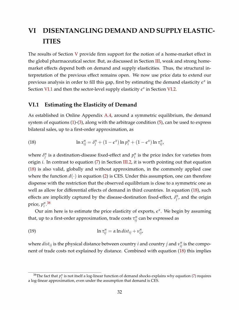
VI DISENTANGLING DEMAND AND SUPPLY ELASTIC-

ITIES

The results of Section V provide firm support for the notion of a home-market effect inthe global pharmaceutical sector. But, as discussed in Section III, weak and strong home-market effects depend both on demand and supply elasticities. Thus, the structural in-terpretation of the previous effect remains open. We now use price data to extend ourprevious analysis in order to fill this gap, first by estimating the demand elasticity εx inSection VI.1 and then the sector-level supply elasticity εs in Section VI.2.

VI.1 Estimating the Elasticity of Demand

As established in Online Appendix A.4, around a symmetric equilibrium, the demandsystem of equations (1)-(3), along with the arbitrage condition (5), can be used to expressbilateral sales, up to a first-order approximation, as

(18) ln xnij = δn

j + (1− εx) ln pni + (1− εx) ln τn

ij ,

where δnj is a destination-disease fixed-effect and pn

i is the price index for varieties fromorigin i. In contrast to equation (7) in Section III.2, it is worth pointing out that equation(18) is also valid, globally and without approximation, in the commonly applied casewhere the function d(·) in equation (2) is CES. Under this assumption, one can thereforedispense with the restriction that the observed equilibrium is close to a symmetric one aswell as allow for differential effects of demand in third countries. In equation (18), sucheffects are implicitly captured by the disease-destination fixed-effect, δn

j , and the originprice, pn

i .38

Our aim here is to estimate the price elasticity of exports, εx. We begin by assumingthat, up to a first-order approximation, trade costs τn

ij can be expressed as

(19) ln τnij = α ln distij + νn

ij,

where distij is the physical distance between country i and country j and νnij is the compo-

nent of trade costs not explained by distance. Combined with equation (18) this implies

38The fact that pni is not itself a log-linear function of demand shocks explains why equation (7) requires

a log-linear approximation, even under the assumption that demand is CES.

32

the following gravity equation relationship between bilateral sales and bilateral distance

(20) ln xnij = δn

j + δni + ρ ln distij + χn

ij

with ρ ≡ (1− εx)α, χnij ≡ (1− εx)νn

ij, and δni representing an origin-disease fixed-effect.

We estimate ρ in this equation via OLS. Our estimate of ρ is reported in Table 9, column(1). As is commonly found in estimates of the gravity equation (20), bilateral distancehas a negative and statistically significant impact on bilateral drug sales in this setting.But the estimated effect of distance on trade, ρ = −0.324, is about three times smaller(in absolute value) than typical estimates from trade data in other sectors. For example,Head and Mayer (2013) report a preferred distance elasticity of −0.89. This is perhapsto be expected, given the relatively low weight-to-value of pharmaceutical products andgiven that our data track total foreign sales (not just exports).

Because the parameter ρ captures a mixture of the demand elasticity εx and the distance-cost elasticity α, we turn to micro-data on the producer prices of individual drug varietiesin order to separate the two.39 In particular, for any individual variety of a drug ω withinthe class of drugs that treat disease n, suppose that prices satisfy the variety-level analogof the non-arbitrage condition in equation (5):

(21) pnij(ω) = τn

ij pni (ω).

Combined with equation (19), this implies that we can obtain an unbiased estimate of α

from the following specification

(22) ln pnij(ω) = α ln distij + δn

i (ω) + δnij(ω),

where δni (ω) is a variety fixed-effect and δn

ij(ω) is an error term.40 The basic idea here isthat if a given variety sells in many destination countries, then the extent to which theprices of that disease vary across destinations j that are different distances distij from theproducer’s origin country i identifies α.

The result from estimating equation (22) is reported in column (2) of Table 9. The esti-

39Producer price (ex-factory) values in the IMS MIDAS dataset correspond to the prices received bymanufacturing firms, as opposed to those received by wholesalers or retailers.

40By “variety” we refer, in practice, to the permutation of physiologically active molecules (since somedrugs contain more than one active molecule), interacted with the disease for which the drug is intendedto treat (since, in rare cases, the same molecule can be marketed in separate therapeutical classes), andinteracted with the firm selling the drug.

33

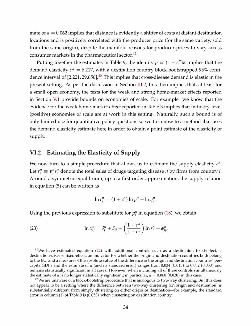
mate of α = 0.062 implies that distance is evidently a shifter of costs at distant destinationlocations and is positively correlated with the producer price (for the same variety, soldfrom the same origin), despite the manifold reasons for producer prices to vary acrossconsumer markets in the pharmaceutical sector.41

Putting together the estimates in Table 9, the identity ρ ≡ (1− εx)α implies that thedemand elasticity εx = 6.217, with a destination country block-bootstrapped 95% confi-dence interval of [2.221, 29.656].42 This implies that cross-disease demand is elastic in thepresent setting. As per the discussion in Section III.2, this then implies that, at least fora small open economy, the tests for the weak and strong home-market effects reportedin Section V.1 provide bounds on economies of scale. For example: we know that theevidence for the weak home-market effect reported in Table 3 implies that industry-level(positive) economies of scale are at work in this setting. Naturally, such a bound is ofonly limited use for quantitative policy questions so we turn now to a method that usesthe demand elasticity estimate here in order to obtain a point estimate of the elasticity ofsupply.

VI.2 Estimating the Elasticity of Supply

We now turn to a simple procedure that allows us to estimate the supply elasticity εs.Let rn

i ≡ pni sn

i denote the total sales of drugs targeting disease n by firms from country i.Around a symmetric equilibrium, up to a first-order approximation, the supply relationin equation (5) can be written as

ln rni = (1 + εs) ln pn

i + ln ηni .

Using the previous expression to substitute for pni in equation (18), we obtain

(23) ln xnij = δn

j + δij +

(1− εx

1 + εs

)ln rn

i + φnij,

41We have estimated equation (22) with additional controls such as a destination fixed-effect, adestination-disease fixed-effect, an indicator for whether the origin and destination countries both belongto the EU, and a measure of the absolute value of the difference in the origin and destination countries’ per-capita GDPs and the estimate of α (and its standard error) ranges from 0.034 (0.015) to 0.082 (0.030) andremains statistically significant in all cases. However, when including all of these controls simultaneouslythe estimate of α is no longer statistically significant; in particular, α = 0.008 (0.020) in this case.

42We are unaware of a block-bootstrap procedure that is analogous to two-way clustering. But this doesnot appear to be a setting where the difference between two-way clustering (on origin and destination) issubstantially different from simply clustering on either origin or destination—for example, the standarderror in column (1) of Table 9 is (0.053) when clustering on destination country.

34

with δij representing an origin-destination fixed-effect and φnij ≡ χn

ij − χ̄nij −

(1−εx

1+εs

)ln ηn

ian error term. Naturally, this expression, which relates bilateral destination sales to totalorigin sales, involves a mixture of the demand elasticity εx in the destination and thesupply elasticity at the origin εs. Armed with an estimate of the demand elasticity εx

from Section VI.1, an estimate of(

1−εx

1+εs

)from equation (23) allows us to disentangle the

two.OLS estimates of equation (23) would be biased because both the supply shock ηn

i andunobserved trade costs χn

ij in the error term φnij contribute to total sales rn

i . But for alldestination observations j 6= i, an exogenous shifter of demand at the origin country i(such as the predicted disease burden variable PDBn

i introduced in equation 14) can beused as a valid instrumental variable for rn

i .43 Such an IV estimation procedure identifies(1−εx

1+εs

).

Table 10 reports estimates from specification (23). We begin in column (1) by report-ing the first-stage regression of ln rn

i on ln PDBni , conditional on origin-destination and

destination-disease fixed-effects. That predicted disease burden is strongly correlatedwith total sales (the F-statistic on this excluded instrument is equal to 128.4, the squareof the t-statistic from column 1) should come as no surprise given the results in Table3.44 Column (2) then reports the OLS estimate of equation (23) and column (3) the corre-sponding IV estimate.45 This (statistically significant) IV estimate implies that

(1−εx

1+εs

)=

0.764. Given our estimate of εx = 6.217 from above, this implies that εs = −7.833 (witha destination country block-bootstrapped 95% confidence interval of [−43.744,−3.565]).As expected, given the bounds implied by the weak home-market effect discussed above,the estimated industry-level supply curve in this setting is downward-sloping, indicatingthe presence of increasing returns to scale.

How does this estimate of εs compare to those in prior work? Both empirical andtheoretical findings offer points of reference. From the empirical literature, one strandaims to estimate industry-level economies of scale directly, via industry-level productionfunctions. A prominent estimate (pooled among all U.S. manufacturing sectors, so unfor-

43Because rni ≡ ∑j xn

ij, equation (23) is a log-linear analog of the canonical peer effects regression dis-cussed in, for example, Manski (1993)—where the regressor of interest is the sum (or mean) of the depen-dent variable within some peer group. As is well known, identification of such peer effects is impossiblewithout instruments that shift the actions of an agent’s peers (and hence potentially also the sum of allpeers’ actions) but do not affect the agent’s own payoff function directly. Our instrument, PDBn

i , plays ananalogous role here (given our focus on observations for which j 6= i).

44Indeed, the test of the weak home-market effect—specifically, column (2) in Table 3—is the reduced-form associated with our IV estimation procedure.

45The fact that the OLS estimate in column (2) is smaller than the IV estimate in column (3) is consistentwith downward-sloping supply curves since when εs < −1 (and given elastic demand, εx > 1) the errorterm φn

ij in equation (23) depends negatively on the supply shock ηni .

35

tunately not available for the pharmaceutical sector alone) from Basu and Fernald (1997)estimates industry-level economies of scale that generate an industry-level supply curvewith εs = −4.45. A second strand, initiated by Antweiler and Trefler (2002), uses patternsof comparative advantage revealed in international trade data to infer relative costs foreach country-industry, and then estimates the extent to which those inferred costs dependon scale. For the pharmaceutical industry Antweiler and Trefler’s (2002) estimates implyεs = −4.27. Since lower supply elasticities in absolute value imply larger effects of quan-tity on producer prices, both of these estimates imply somewhat stronger economies ofscale than found in our estimate of εs =−7.833.46 That said, neither of these estimatesis based on an empirical strategy that isolates variation that stems from the demand sidealone and yet is powerful enough to circumvent weak instrument concerns.47

The influential model of Krugman (1980) also provides a clear benchmark. As dis-cussed in Section III.3, this model is a special case in which there is a particularly starkconnection between industry-level supply and demand elasticities: εs = −εx. This im-plies that

(1−εx

1+εs

), the coefficient reported in column (3) of Table 10, should be equal to

one. Instead our IV estimate is equal to 0.764 , or about 25% smaller. While the reportedp-value demonstrates that the particular parameter value assumed in Krugman (1980) isrejected at the five percent level, our estimate is certainly closer to this benchmark valuethan to the constant-returns extreme in which εs = ∞ (and hence the coefficient in column3 would be equal to zero).

VII CONCLUDING REMARKS

Since the home-market effect hypothesized by Linder (1961) and formalized by Krugman(1980) is about the causal effect of cross-country differences in demand on the pattern of

46One possible reason for the stronger industry-level economies of scale found in these earlier studies,relative to ours, is that they are obtained from settings with more aggregate notions of an industry (a repre-sentative manufacturing sector in Basu and Fernald, 1997 or the entire pharmaceutical sector in Antweilerand Trefler, 2002) than that used here (a representative disease class within the pharmaceutical sector).

47A third example of work that attempts to estimate industry-level economies of scale is due to Shea(1993), who finds that the industry-level supply curve slopes upwards in the pharmaceutical industry. Thisapproach (when applied, for example, to the pharmaceutical sector) uses input-output table informationto find a downstream sector that buys a substantial share of its inputs from the pharmaceutical sector, butwhich sources only a small share of its other inputs from sectors that themselves are not used substan-tially as inputs in the pharmaceutical sector. When estimating an inverse supply curve, output in such adownstream sector can then be employed as a demand-side instrumental variable for output in the phar-maceutical sector under the assumption that the two sectors do not face correlated demand shocks. Ourfinding of a downward-sloping supply curve derives from a different orthogonality condition, namely thatpredicted disease burden in the origin country is uncorrelated with unobserved determinants of demandin the destination, after controlling for both destination-disease and origin-destination fixed effects.

36

international specialization, any empirical test of this phenomenon requires exogenousdemand variation. In this paper, we have focused on the global pharmaceutical industryas a way to obtain such variation. Our empirical strategy builds on the basic observationthat countries whose populations, because of exogenous demographic characteristics, aremore likely to suffer from particular diseases are also more likely to have high demandfor drugs targeting those diseases.

We have conducted tests of two different notions of the home-market effect. The firsttest, which is based on what we have referred to as the weak home-market effect, inves-tigates whether countries tend to sell more abroad in sectors for which they have largerdomestic markets. In the present context, this boils down to estimating whether the elas-ticity of a country’s foreign sales with respect to its demographically predicted diseaseburden is positive. In line with the work of Linder (1961), the answer is a resounding yes.In short, the more we die (at home), the more we sell (abroad).

Our second test, defined by what we have referred to as the strong home-market ef-fect, explores whether the previous effect can be important enough to turn countries withlarger demand for some products into net sellers of those products, a stronger implicationof Krugman’s (1980) monopolistically competitive model. Our baseline results speak infavor of the strong home-market effect taking place in the pharmaceutical sector, though,in comparison with the weak home-market effect, we are not able to reject the null of nostrong home-market effect in some of our specifications.

To delve further into the economic determinants of the home-market effect, we haveconcluded our analysis by estimating demand and supply elasticities in the pharma-ceutical industry. Our estimates point towards the home-market effect being driven bysubstantial economies of scale at the sector-level rather than a low elasticity of demand.Quantitatively, we have estimated a supply elasticity that is about three-quarters the sizeof what a monopolistically competitive model, like Krugman (1980), would predict. Re-cent quantitative work on international trade and economic geography has typically as-sumed, without attempting to estimate, economies of scale that are either zero, as in Eatonand Kortum (2002), or of Krugman’s (1980) magnitude. In our context, both extremes arerejected by the data. Our analysis, however, demonstrates how a single supply-side pa-rameter can nest these two cases, and how a plausibly exogenous demand shifter can letthe data speak freely to this parameter’s value.

Finally, we note that our results provide empirical support to the heterodox view thatimport protection may lead to export promotion, at least within the context of a specific,but important industry. Of course, whether such promotion is welfare improving or notmay depend on the underlying sources of economies of scale, a matter on which our

37

analysis remains silent.

Costinot: MIT, CEPR, and NBERDonaldson: MIT, CEPR, and NBERKyle: Mines ParisTech and CEPRWilliams: MIT and NBER

38

References

Acemoglu, Daron and Joshua Linn, “Market size in innovation: Theory and evidencefrom the pharmaceutical industry,” Quarterly Journal of Economics, 2004, 119 (3), 1049–1090.

Amiti, Mary, “Inter-industry trade in manufactures: does country size matter?,” Journalof Intermational Economics, 1998, 44, 231–255.

Antweiler, Werner and Daniel Trefler, “Increasing Returns and All That: A View fromTrade,” American Economic Review, 2002, 92 (1), 93–119.

Arthur, Brian W., “Silicon Valley locational clusters: When do increasing returns implymonopoly?,” Mathematical Social Sciences, 1990, 19, 235–51.

Azoulay, Pierre, Joshua S. Graff-Zivin, Danielle Li, and Bhaven N. Sampat, “PublicR&D Investments and Private-sector Patenting: Evidence from NIH Funding Rules,”Review of Economic Studies, 2018, forthcoming.

Basu, Susanto and John G. Fernald, “Returns to Scale in U.S. Production: Estimates andImplications,” Journal of Political Economy, 1997, 105 (2), 249–283.

Behrens, Kristian, Andrea R. Lamorgese, Gianmarco Ottaviano, and TakatoshiTabuchi, “Beyond the home market effect: Market size and specialization in a multi-country world,” Journal of International Economics, 2009, 79 (2), 259–265.

Bilir, Kamran and Eduardo Morales, “Innovation in the Global Firm,” NBER workingpaper 22160, 2018.

Brulhart, Marius and Federico Trionfetti, “A test of trade theories when expenditure ishome biased,” European Economic Review, 2009, 53 (7), 830–845.

Cameron, A. Colin, Jonah B. Gelbach, and Douglas L. Miller, “Robust Inference WithMultiway Clustering,” Journal of Business and Economic Statistics, 2011, 29 (2), 238–249.

Caron, Justin, Thibault Fally, and Ana Cecilia Fieler, “Home-market effects on innova-tion,” mimeo UC Berkeley, 2015.

Chor, Davin, “Unpacking Sources of Comparative Advantage: A Quantitative Ap-proach,” Journal of International Economics, 2010, 82 (2), 152–167.

39

Cleave, TL, Peptic Ulcer: A New Approach to its Causation, Prevention, and Arrest, Based onHuman Evolution, Bristol: Great Britain: John Wright and Sons Ltd, 1962.

Costinot, Arnaud, Dave Donaldson, and Ivana Komunjer, “What Goods Do CountriesTrade? A Quantitative Exploration of Ricardo’s Ideas,” Review of Economic Studies, 2012,79 (2), 581–608.

, , Margaret Kyle, and Heidi Williams, “The More We Die, The More We Sell? ASimple Test of the Home-Market Effect,” mimeo MIT, 2016.

Crozet, Mathieu and Federico Trionfetti, “Trade costs and the home market effect,” Jour-nal of Intermational Economics, 2008, 76, 309–321.

Davis, Donald R., “The home market, trade and industrial structure,” American EconomicReview, 1998, 88 (5), 1264–1276.

and David Weinstein, “Does Economic Geography Matter for International Special-ization?,” NBER Working Paper 5706, 1996.

and , “Economic geography and regional production structure: an empirical inves-tigation,” European Economic Review, 1999, 43, 379–407.

and , “Market access, economic geography and comparative advantage: an empiricaltest,” Journal of Intermational Economics, 2003, 59, 1–23.

DellaVigna, Stefano and Joshua M. Pollet, “Demographics and Industry Returns,”American Economic Review, 2007, 97 (5), 1667–1702.

Dingel, Jonathan I., “The Determinants of Quality Specialization,” Review of EconomicStudies, 2016, 84 (4), 1551–1582.

Eaton, Jonathan and Samuel Kortum, “Technology, Geography and Trade,” Econometrica,2002, 70 (5), 1741–1779.

Ethier, Wilfred J., “Decreasing Costs in International Trade and Frank Graham’s Argu-ment for Protection,” Econometrica, 1982, 50 (5), 1243–1268.

Fabrizio, Kira R. and L. G. Thomas, “The Impact of Local Demand on Innovation in aGlobal Industry,” Strategic Management Journal, 2012, 33 (1), 42–64.

Fajgelbaum, Pablo, Gene M. Grossman, and Elhanan Helpman, “Income Distribution,Product Quality, and International Trade,” Journal of Political Economy, 2011, 119 (4),721–765.

40

, , and , “A Linder Hypothesis for Foreign Direct Investment,” Review of EconomicStudies, 2015, 82, 83–121.

Feenstra, Robert C., James R. Markusen, and Andrew K. Rose, “Using the GravityEquation to Differentiate among Alternative Theories of Trade,” Canadian Journal of Eco-nomics, 2001, 34 (2), 430–447.

Fujita, Masahisa, Paul R. Krugman, and Anthony Venables, The Spatial Economy: Cities,Regions, and International Trade, MIT press, 2001.

Gali, Jordi and Tommaso Monacelli, “Monetary Policy and Exchange Rate Volatility ina Small Open Economy,” Review of Economic Studies, 2005, 72, 707–734.

Hanson, Gordon H. and Chong Xiang, “The home market effect and bilateral trade pat-terns,” American Economic Review, 2004, 94 (4), 1108–1129.

Hara, Takuji, Innovation in the Pharmaceutical Industry: The Process of Drug Discovery andDevelopment, Cheltenham: UK: Edward Elgar, 2003.

Head, Keith and John Ries, “Increasing Returns versus National Product Differentiationas an Explanation for the Pattern of U.S.-Canada Trade,” American Economic Review,2001, 91 (4), 858–876.

and Thierry Mayer, “The Empirics of Agglomeration and Trade,” in J.V. Hendersonand J.F. Thisse, eds., Handbook of Regional and Urban Economic, Vol. 4, Amsterdam: Hol-land: Elsevier, 2004.

and , “The erosion of colonial trade linkages after independence,” Journal of Interna-tional Economics, 2010, 81 (1), 1–14.

and , “Gravity Equations: Toolkit, Cookbook, Workhorse,” in Gita Gopinath, El-hanan Helpman, and Kenneth Rogoff, eds., Handbook of International Economics, Vol. 4,Elsevier, 2013.

, , and John Ries, “On the Pervasiveness of Home Market Effects,” Economica, 2002,69, 371–390.

Helpman, Elhanan and Paul R. Krugman, Market Structure and Foreign Trade: IncreasingReturns, Imperfect Competition, and the International Economy, Cambridge, Massachusetts:MIT Press, 1985.

and , Trade Policy and Market Structure, Cambridge, Massachussetts: MIT Press, 1989.

41

Holmes, Thomas J. and John J. Stevens, “Does home market size matter for the patternof trade?,” Journal of International Economics, 2005, 65, 489–505.

Jaravel, Xavier, “The Unequal Gains from Product Innovations: Evidence from the U.S.Retail Sector,” Quarterly Journal of Economics, 2018, forthcoming.

Krugman, Paul R., “Scale Economies, Product Differentiation, and the Pattern of Trade,”The American Economic Review, 1980, 70 (5), 950–959.

, “Import protection as export promotion: international competition in the presence ofoligopoly and economies of scale,” in Henryk Kierzkowski, ed., Monopolistic competitionin international trade, Oxford University Press, 1984.

Lichtenberg, Frank R., “The Allocation of Publicly Funded Biomedical Research,” inDavid M. Cutler and Ernst R. Berndt, eds., Medical Care Output and Productivity, Uni-versity of Chicago Press, 2001, pp. 565–590.

Linder, Staffan B., An Essay on Trade and Transformation, Uppsala: Almqvist and Wiksells,1961.

Lundback, Erik J. and Johan Torstensson, “Demand, comparative advantage and eco-nomic geography in international trade: Evidence from the OECD,” Review of WorldEconomics, 1998, 134 (2), 230–249.

Manski, Charles F., “Identification of Endogenous Social Effects: The Reflection Prob-lem,” Review of Economic Studies, 1993, 60 (3), 531–542.

Matsuyama, Kiminori, “The Home Market Effect and the Pattern of Trade Between Richand Poor Countries,” mimeo Northwestern University, 2015.

, “Geographical Advantage: Home Market Effect in a Multi-Region World,” Research inEconomics, 2017, 71 (4), 740–758.

Ramondo, Natalia and Andres Rodríguez-Clare, “Trade, Multinational Production, andthe Gains from Openness,” Journal of Political Economy, 2013, 121 (2), 273–322.

Scott Morton, Fiona and Margaret Kyle, “Markets for Pharmaceutical Products,” inThomas G. Mcguire Mark V. Pauly and Pedro P. Barros, eds., Handbook of Health Eco-nomics, Vol. 2, Elsevier, 2012.

Shea, John, “Do Supply Curves Slope Up?,” Quarterly Journal of Economics, 1993, 108 (1),1–32.

42

Thomas, Lacy Glenn, “Implicit Industrial Policy: The Triumph of Britain and the Failureof France in Global Pharmaceuticals,” Industrial and Corporate Change, 1994, 3 (2), 451–489.

Trionfetti, Federico, “Using Home-Biased Demand to Test Trade Theories,” Review ofWorld Economics, 2001, 137 (3), 404–426.

Vernon, Raymond, “International Investment and International Trade in the Product Cy-cle,” Quarterly Journal of Economics, 1966, 80 (2), 190–207.

Weder, Rolf, “Comparative home-market advantage: An empirical analysis of Britishand American exports,” Review of World Economics, 2003, 139 (2), 220–247.

43

Table I: Top 10 Countries in Terms of Sales

Share of Share of world Number of firmsworld sales (%) expenditures (%) headquartered

Country (1) (2) (3)

USA 37.12 42.10 356Switzerland 12.68 0.61 35Japan 11.62 12.67 53United Kingdom 10.67 2.67 80Germany 6.77 4.68 94France 6.51 4.34 58India 2.29 1.61 292China, Mainland 2.18 3.74 524Canada 1.36 2.57 46Italy 1.35 3.35 68

Table II: Top 10 Diseases in Terms of Sales

AverageShare of Number of Herfindahlworld origin index across

sales (%) countries destinations

Disease class (WHO system) (1) (2) (3)

Other infectious diseases 8.62 55 0.08Hypertensive heart disease 6.56 55 0.10Other cardiovascular diseases 6.30 55 0.13Ischaemic heart disease 5.99 54 0.14Other neoplasms 5.80 52 0.12Diabetes mellitus 4.75 54 0.15Rheumatoid arthritis 4.55 49 0.23Other genitourinary system diseases 3.97 52 0.14Chronic obstructive pulmonary dis. 3.50 49 0.27Schizophrenia 3.27 52 0.17

44

Table III: Test of the Home-Market Effect (Baseline)

log (bilateral sales)

(1) (2) (3)

log (PDB, destination) 0.520 0.545(0.097) (0.107)

log (PDB, origin) 0.947 0.928(0.174) (0.123)

p-value for H0 : β̃X ≤ 0 0.000*** 0.000***p-value for H0 : β̃X ≤ β̃M 0.018**

Origin × disease FE XDestination × disease FE XDisease FE X

Adjusted R2 0.630 0.563 0.540Observations 18,756 18,905 19,150

Notes: OLS estimates of equation (16). Predicted disease burden (PDBni ) is constructed from an interaction

between the global (leaving out country i) disease burden by demographic group in disease n, and thesize of each demographic group in country i. All regressions omit the bilateral sales observation for homesales (i.e. where i = j) and control for origin-times-destination fixed-effects. The number of observationsdiffers across columns due to omission of observations that are completely accounted for by the includedfixed-effects. Standard errors in parentheses are two-way clustered at origin and destination country levels.p-values are based on F-test of the stated H0. *** p<0.01, ** p<0.05. A p-value of “0.000” refers to one below0.0005.

45

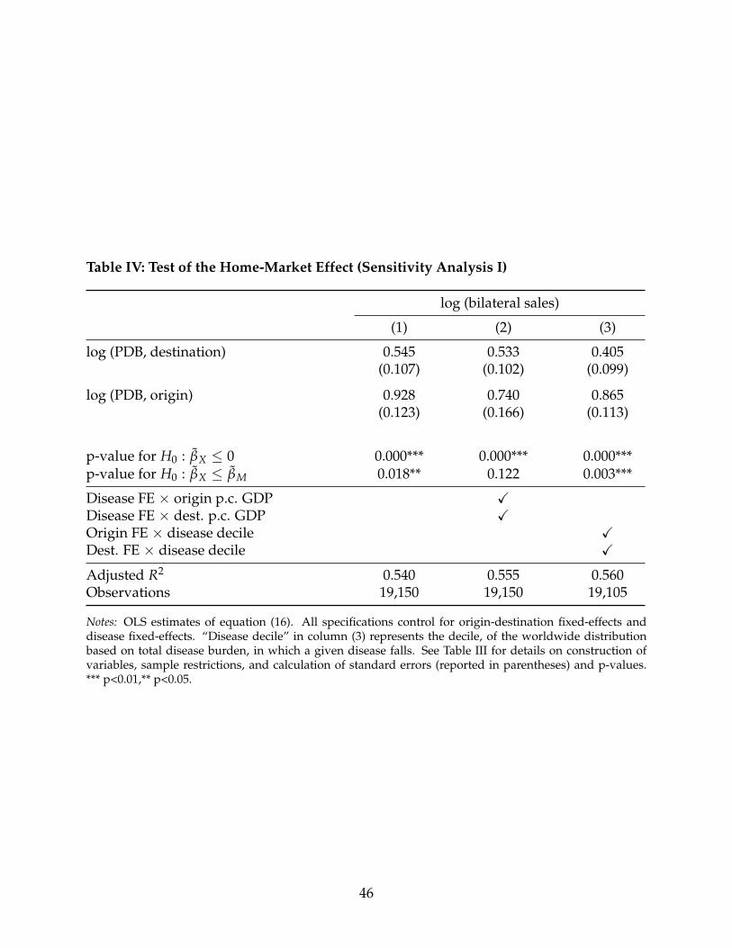
Table IV: Test of the Home-Market Effect (Sensitivity Analysis I)

log (bilateral sales)

(1) (2) (3)

log (PDB, destination) 0.545 0.533 0.405(0.107) (0.102) (0.099)

log (PDB, origin) 0.928 0.740 0.865(0.123) (0.166) (0.113)

p-value for H0 : β̃X ≤ 0 0.000*** 0.000*** 0.000***p-value for H0 : β̃X ≤ β̃M 0.018** 0.122 0.003***

Disease FE × origin p.c. GDP XDisease FE × dest. p.c. GDP XOrigin FE × disease decile XDest. FE × disease decile X

Adjusted R2 0.540 0.555 0.560Observations 19,150 19,150 19,105

Notes: OLS estimates of equation (16). All specifications control for origin-destination fixed-effects anddisease fixed-effects. “Disease decile” in column (3) represents the decile, of the worldwide distributionbased on total disease burden, in which a given disease falls. See Table III for details on construction ofvariables, sample restrictions, and calculation of standard errors (reported in parentheses) and p-values.*** p<0.01,** p<0.05.

46

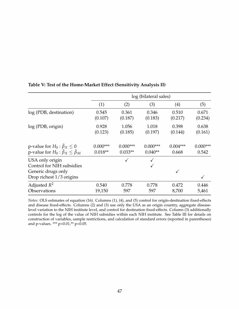
Table V: Test of the Home-Market Effect (Sensitivity Analysis II)

log (bilateral sales)

(1) (2) (3) (4) (5)

log (PDB, destination) 0.545 0.361 0.346 0.510 0.671(0.107) (0.187) (0.183) (0.217) (0.234)

log (PDB, origin) 0.928 1.056 1.018 0.398 0.638(0.123) (0.185) (0.197) (0.144) (0.161)

p-value for H0 : β̃X ≤ 0 0.000*** 0.000*** 0.000*** 0.004*** 0.000***p-value for H0 : β̃X ≤ β̃M 0.018** 0.033** 0.040** 0.668 0.542

USA only origin X XControl for NIH subsidies XGeneric drugs only XDrop richest 1/3 origins X

Adjusted R2 0.540 0.778 0.778 0.472 0.446Observations 19,150 597 597 8,700 5,461

Notes: OLS estimates of equation (16). Columns (1), (4), and (5) control for origin-destination fixed-effectsand disease fixed-effects. Columns (2) and (3) use only the USA as an origin country, aggregate disease-level variation to the NIH institute level, and control for destination fixed-effects. Column (3) additionallycontrols for the log of the value of NIH subsidies within each NIH institute. See Table III for details onconstruction of variables, sample restrictions, and calculation of standard errors (reported in parentheses)and p-values. *** p<0.01,** p<0.05.

47

Table VI: Test of the Home-Market Effect (Sensitivity Analysis III)

log (bilateral sales)

(1) (2) (3) (4)

log (PDB, destination) 0.545 0.537 0.610 0.542(0.107) (0.115) (0.087) (0.107)

log (PDB, origin) 0.928 0.941 0.843 0.928(0.123) (0.147) (0.166) (0.127)

p-value for H0 : β̃X ≤ 0 0.000*** 0.000*** 0.000*** 0.000***p-value for H0 : β̃X ≤ β̃M 0.018** 0.033** 0.134 0.019**

Sample of only ij obs. with distij ≥ – 1,000 km 2,000 km –Control for ∑k 6=j ln PDBn

k · dist−1kj X

Control for ∑k 6=i ln PDBnk · dist−1

ik X

Adjusted R2 0.540 0.540 0.551 0.540Observations 19,150 16,405 13,141 19,150

Notes: OLS estimates of equation (16). All specifications control for origin-destination fixed-effects and dis-ease fixed-effects. See Table III for details on construction of variables, sample restrictions, and calculationof standard errors (reported in parentheses) and p-values. *** p<0.01,** p<0.05.

48

Table VII: Test of the Home-Market Effect (Sensitivity Analysis IV)

log (bilateral sales)

(1) (2) (3) (4) (5)

log (PDB, destination) 0.545 −0.007 0.573 0.547 0.514(0.107) (0.460) (0.265) (0.102) (0.104)

log (PDB, origin) 0.928 0.726 0.823 0.785 0.843(0.123) (0.285) (0.201) (0.104) (0.098)

p-value for H0 : β̃X ≤ 0 0.000*** 0.010** 0.000*** 0.000*** 0.000***p-value for H0 : β̃X ≤ β̃M 0.018** 0.098* 0.198 0.061* 0.023**

EU destinations only XBelow median FDI share XPDB with 1996 demographics XHome sales (Xn

ii) obs. incl. X

Adjusted R2 0.540 0.538 0.459 0.539 0.563Observations 19,150 7,223 5,081 19,150 21,291

Notes: OLS estimates of equation (16). All specifications control for origin-destination fixed-effects and dis-ease fixed-effects. See Table III for details on construction of variables, sample restrictions, and calculationsof standard errors (reported in parentheses) and p-values. *** p<0.01,** p<0.05, * p<0.1.

49

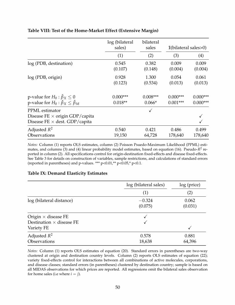
Table VIII: Test of the Home-Market Effect (Extensive Margin)

log (bilateral bilateralsales) sales 1(bilateral sales>0)

(1) (2) (3) (4)

log (PDB, destination) 0.545 0.382 0.009 0.009(0.107) (0.148) (0.004) (0.004)

log (PDB, origin) 0.928 1.300 0.054 0.061(0.123) (0.534) (0.013) (0.013)

p-value for H0 : β̃X ≤ 0 0.000*** 0.008*** 0.000*** 0.000***p-value for H0 : β̃X ≤ β̃M 0.018** 0.066* 0.001*** 0.000***

PPML estimator XDisease FE × origin GDP/capita XDisease FE × dest. GDP/capita X

Adjusted R2 0.540 0.421 0.486 0.499Observations 19,150 64,728 178,640 178,640

Notes: Column (1) reports OLS estimates, column (2) Poisson Psuedo-Maximum Likelihood (PPML) esti-mates, and columns (3) and (4) linear probability model estimates, based on equation (16). Pseudo-R2 re-ported in column (2). All specifications control for origin-destination fixed-effects and disease fixed-effects.See Table 3 for details on construction of variables, sample restrictions, and calculations of standard errors(reported in parentheses) and p-values. *** p<0.01,** p<0.05,* p<0.1.

Table IX: Demand Elasticity Estimates

log (bilateral sales) log (price)

(1) (2)

log (bilateral distance) −0.324 0.062(0.075) (0.031)

Origin × disease FE XDestination × disease FE XVariety FE X

Adjusted R2 0.578 0.881Observations 18,638 64,396

Notes: Column (1) reports OLS estimates of equation (20). Standard errors in parentheses are two-wayclustered at origin and destination country levels. Column (2) reports OLS estimates of equation (22);variety fixed-effects control for interactions between all combinations of active molecules, corporations,and disease classes; standard errors (in parentheses) clustered by destination country; sample is based onall MIDAS observations for which prices are reported. All regressions omit the bilateral sales observationfor home sales (i.e where i = j).

50

Table X: Supply Elasticity Estimates

log (total sales) log (bilateral sales)

OLS OLS IV(1) (2) (3)

log (PDB) 1.241(0.110)

log (total sales) 0.669 0.764(0.052) (0.116)

p-value for H0 :(

1−εx

1+εs

)= 1 0.048**

Adjusted R2 0.789 0.629 0.627Observations 18,905 18,905 18,905

Notes: Column (2) reports the OLS estimate, and column (3) the IV estimate, of equation (22). Column(1) reports the corresponding first-stage specification. The instrumental variable is log(PDB) in the origincountry. All regressions omit the bilateral sales observation for home sales (i.e where i = j) and controlfor origin-destination and destination-disease fixed-effects. Standard errors in parentheses are two-wayclustered at origin and destination country levels. p-value is based on F-test of H0. ** p<0.05.

51