Embed Size (px)
Citation preview

QUANTUM MONTE CARLO METHODS FOR FERMIONIC SYSTEMS:BEYOND THE FIXED-NODE APPROXIMATION
A THESIS SUBMITTED TOTHE GRADUATE SCHOOL OF NATURAL AND APPLIED SCIENCES
OFMIDDLE EAST TECHNICAL UNIVERSITY
BY
NAZIM DUGAN
IN PARTIAL FULFILLMENT OF THE REQUIREMENTSFOR
THE DEGREE OF DOCTOR OF PHILOSOPHYIN
PHYSICS
AUGUST 2010

Approval of the thesis:
QUANTUM MONTE CARLO METHODS FOR FERMIONIC SYSTEMS:
BEYOND THE FIXED-NODE APPROXIMATION
submitted by NAZIM DUGAN in partial fulfillment of the requirements for the degree ofDoctor of Philosophy in Physics Department, Middle East Technical University by,
Prof. Dr. Canan OzgenDean, Graduate School of Natural and Applied Sciences
Prof. Dr. Sinan BilikmenHead of Department, Physics
Prof. Dr. Sakir ErkocSupervisor, Physics Department, METU
Examining Committee Members:
Prof. Dr. Bilal TanatarPhysics Department, Bilkent University
Prof. Dr. Sakir ErkocPhysics Department, METU
Prof. Dr. Umit KızılogluPhysics Department, METU
Prof. Dr. Ramazan SeverPhysics Department, METU
Assist. Prof. Dr. Hande ToffoliPhysics Department, METU
Date:

I hereby declare that all information in this document has been obtained and presentedin accordance with academic rules and ethical conduct. I also declare that, as requiredby these rules and conduct, I have fully cited and referenced all material and results thatare not original to this work.
Name, Last Name: NAZIM DUGAN
Signature :
iii

ABSTRACT
QUANTUM MONTE CARLO METHODS FOR FERMIONIC SYSTEMS:BEYOND THE FIXED-NODE APPROXIMATION
Dugan, Nazım
Ph.D., Department of Physics
Supervisor : Prof. Dr. Sakir Erkoc
August 2010, 61 pages
Developments are made on the quantum Monte Carlo methods towards increasing the pre-
cision and the stability of the non fixed-node projector calculations of fermions. In the first
part of the developments, the wavefunction correction scheme, which was developed to in-
crease the precision of the diffusion Monte Carlo (DMC) method, is applied to non fixed-node
DMC to increase the precision of such fermion calculations which do not have nodal error.
The benchmark calculations indicate a significant decrease of statistical error due to the us-
age of the correction scheme in such non fixed-node calculations. The second part of the
developments is about the modifications of the wavefunction correction scheme for having
a stable non fixed-node DMC algorithm for fermions. The minus signed walkers of the non
fixed-node calculations are avoided by these modifications in the developed stable algorithm.
However, the accuracy of the method decreases, especially for larger systems, as a result of
the discussed modifications to overcome the sign instability.
Keywords: electronic structure calculations, quantum Monte Carlo, fermions
iv

OZ
FERMIYONIK SISTEMLER ICIN KUANTUM MONTE CARLO YONTEMLERI:SABIT DUGUM YAKINLASTIRMASI OTESI
Dugan, Nazım
Doktora, Fizik Bolumu
Tez Yoneticisi : Prof. Dr. Sakir Erkoc
Agustos 2010, 61 sayfa
Kuantum Monte Carlo yontemleri alanında, sabit dugum yakınlastırması kullanmadan fer-
miyon hesabı yapan difuzyon Monte Carlo (DMC) yonteminin hassasiyet ve kararlılıgını
arttırıcı gelistirmeler yapıldı. Gelistirmelerin ilk bolumunde, difuzyon Monte Carlo yonteminin
hassasiyetini arttırmak icin gelistirilmis olan dalga fonksiyonu duzeltme teknigi, sabit dugumsuz
DMC yontemine, hassasiyeti arttırma amacı ile uygulandı. Yapılan deneme hesaplarında,
dalga fonksiyonu duzeltme teknigi kullanılması sonucu istatistiksel hatalarda buyuk dususler
oldugu goruldu. Gelistirmelerin ikinci bolumu, kararlı bir sabit dugumsuz DMC algorit-
ması gelistirmek amacı ile, dalga fonksiyonu duzeltme teknigi uzerinde yapılan bir takım
degisiklikler hakkındadır. Bu kararlı yontemde, sabit dugumsuz hesaplarda olusan eksi isaretli
yuruyuculer (walkers), acıklanan degisiklikler sayesinde engellendi. Ancak, bu yontemle
elde edilen sonucların dogrulugunun, ozellikle buyuk sistemlerde, eksi isaret kararsızlıgını
engellemek icin yapılan degisiklikler yuzunden azaldıgı sonucuna ulasıldı.
Anahtar Kelimeler: elektronik yapı hesapları, kuantum Monte Carlo, fermiyonlar
v

To my love Nilay
vi

ACKNOWLEDGMENTS
I would like to thank my Supervisor Sakir Erkoc for his endless support in my studies. He
was more than a supervisor for me in the last five years. I would like to thank Dr. Inanc Kanık
for his friendship and collaborations in this thesis work. This work would not be possible
without his non stopping ideas. I would like to thank past and current graduate students of
our group : Dr. Emre Tascı, Dr. Barıs Malcıoglu, Dr. Rengin Pekoz and Deniz Tekin for their
firendships and collaborations. I wish success to all of them in their future academic life. I
would like to thank the professors of METU Physics Department giving a special place to
Hande Toffoli and Bayram Tekin for their supports in this thesis work. I would like to thank
past and current graduate students Kıvanc Uyanık, Nader Ghazanfari, Cagrı Sisman and Cetin
Senturk for the discussions about all branches of physics and also for their friendships. I also
thank my family and my love for supporting me in my personal life.
vii

TABLE OF CONTENTS
ABSTRACT . . . . . . . . . . . . . . . . . . . . . . . . . . . . . . . . . . . . . . . . iv
OZ . . . . . . . . . . . . . . . . . . . . . . . . . . . . . . . . . . . . . . . . . . . . . v
DEDICATION . . . . . . . . . . . . . . . . . . . . . . . . . . . . . . . . . . . . . . vi
ACKNOWLEDGMENTS . . . . . . . . . . . . . . . . . . . . . . . . . . . . . . . . . vii
TABLE OF CONTENTS . . . . . . . . . . . . . . . . . . . . . . . . . . . . . . . . . viii
LIST OF TABLES . . . . . . . . . . . . . . . . . . . . . . . . . . . . . . . . . . . . xi
LIST OF FIGURES . . . . . . . . . . . . . . . . . . . . . . . . . . . . . . . . . . . . xii
CHAPTERS
1 INTRODUCTION . . . . . . . . . . . . . . . . . . . . . . . . . . . . . . . 1
1.1 Schrodinger Equation for Many Electron Systems . . . . . . . . . . 2
1.1.1 Expectation value of an observable . . . . . . . . . . . . . 3
1.1.2 Variational principle . . . . . . . . . . . . . . . . . . . . 3
1.1.3 Indistinguishable particles and the antisymmetry condition 4
1.1.4 Spin and spatial parts of the wavefunction . . . . . . . . . 5
1.1.5 Electronic structure problem . . . . . . . . . . . . . . . . 5
1.2 Quantum Monte Carlo . . . . . . . . . . . . . . . . . . . . . . . . . 7
1.2.1 Statistical sampling and the Metropolis algorithm . . . . . 8
1.2.2 Monte Carlo integration . . . . . . . . . . . . . . . . . . 9
1.2.3 Variational Monte Carlo . . . . . . . . . . . . . . . . . . 9
1.2.4 Diffusion process as random walk . . . . . . . . . . . . . 11
1.2.5 Diffusion Monte Carlo . . . . . . . . . . . . . . . . . . . 12
1.2.6 Importance sampling DMC . . . . . . . . . . . . . . . . . 15
1.2.7 Fermion sign problem (FSP) in DMC . . . . . . . . . . . 17
viii

1.2.8 Fixed-node approximation . . . . . . . . . . . . . . . . . 18
1.3 DMC Beyond the Fixed-node Approximation . . . . . . . . . . . . 19
1.3.1 Released-node technique . . . . . . . . . . . . . . . . . . 19
1.3.2 Plus minus cancellation methods . . . . . . . . . . . . . . 20
1.3.3 Correlated walk of opposite signed walkers . . . . . . . . 21
1.3.4 Non-symmetric guiding functions and the fermion MonteCarlo . . . . . . . . . . . . . . . . . . . . . . . . . . . . 22
1.3.5 Using permutation symemtry . . . . . . . . . . . . . . . . 22
1.3.6 Other Strategies towards the solution of FSP . . . . . . . . 23
1.4 Fermion Trial Wavefunctions . . . . . . . . . . . . . . . . . . . . . 24
2 WAVEFUNCTION CORRECTION SCHEME FOR NON FIXED-NODE DMC 27
2.1 Wavefunction Correction Scheme . . . . . . . . . . . . . . . . . . . 27
2.1.1 Vacuum branchings . . . . . . . . . . . . . . . . . . . . . 29
2.1.2 Amplitude ratio parameter . . . . . . . . . . . . . . . . . 29
2.1.3 Expectation value calculation . . . . . . . . . . . . . . . . 30
2.2 Usage of the Correction Scheme in Non Fixed-Node DMC . . . . . 31
2.2.1 Algorithm details . . . . . . . . . . . . . . . . . . . . . . 32
2.2.2 Parameters . . . . . . . . . . . . . . . . . . . . . . . . . 33
2.2.3 Statistical error analysis . . . . . . . . . . . . . . . . . . 35
2.2.4 Benchmark computations . . . . . . . . . . . . . . . . . . 35
2.2.5 Discussion about the benchmark calculation results . . . . 41
2.3 Stable Non Fixed-Node Algorithm Using Correction Scheme . . . . 43
2.3.1 Downwards shift of the trial wavefunction . . . . . . . . . 43
2.3.2 Vacuum branchings at walker positions . . . . . . . . . . 44
2.3.3 Two permutation cells and two reference energies . . . . . 46
2.3.4 Harmonic fermion calculations using the stable algorithm . 47
3 CONCLUSIONS . . . . . . . . . . . . . . . . . . . . . . . . . . . . . . . . 50
REFERENCES . . . . . . . . . . . . . . . . . . . . . . . . . . . . . . . . . . . . . . 52
APPENDICES
ix

A PROOF OF THE VARIATIONAL PRINCIPLE . . . . . . . . . . . . . . . . 57
CURRICULUM VITAE . . . . . . . . . . . . . . . . . . . . . . . . . . . . . . . . . 59
x

LIST OF TABLES
TABLES
Table 2.1 Correction scheme computation results for two harmonic fermions. d: space
dimension, ε1,ε2: disturbance parameter values, Ec: calculated energy expectation
value using the correction scheme, EGS : true value of the fermionic ground state
energy, ET : trial wavefunction energy (all energies are given in dimensionless
units), Nw: stabilized number of walkers from each sign, rn: ratio of the trial
wavefunction normalization to the number of walkers from each sign, rt: ratio of
the comparison case computation time to the correction scheme computation time. 37
xi

LIST OF FIGURES
FIGURES
Figure 1.1 Illustration of the imaginary time evolution in DMC method. Adapted from
the review article of Foulkes et al. [8]. . . . . . . . . . . . . . . . . . . . . . . . 14
Figure 2.1 Dashed Line: Trial wavefunction ΨT (x), Solid Line: Ground state wave-
function ΨGS (x), Dotted Line: Difference function ΨGS (x) − ΨT (x). . . . . . . . 28
Figure 2.2 Wavefunction plots for correction scheme DMC computation of the two
harmonic fermions in 1D. TOP: Trial wavefunction. MIDDLE: Difference be-
tween the true fermionic ground state and the trial wavefunction. BOTTOM:
Average walker distribution during the DMC computation. . . . . . . . . . . . . . 38
Figure 2.3 Calculated energy expectation value versus normalization ratio parameter
rn for harmonic fermions in 1D. . . . . . . . . . . . . . . . . . . . . . . . . . . . 39
Figure 2.4 He atom 1s2s 3S state trial wavefunction (Eq. 2.11) cross section on r1 =
2 r2 surface. Node crossing is seen at r2 = 0.5 a.u. . . . . . . . . . . . . . . . . . 40
Figure 2.5 Downwards shift of the trial wavefunction ΨT (x). Dashed Line: Shifted
trial wavefunction ΨsT (x), Solid Line: Ground state wavefunction ΨGS (x), Dotted
Line: Difference function ΨGS (x) − ΨsT (x). . . . . . . . . . . . . . . . . . . . . . 43
Figure 2.6 Position dependent shift of the trial wavefunction. Dashed Line: Shifted
trial wavefunction ΨsT (x), Solid Line: Ground state wavefunction ΨGS (x). . . . . 44
Figure 2.7 Wavefunction plots for two harmonic fermions in 1D. Horizontal axes
x1, x2 are the positions of the two fermions. TOP: Difference between the true
fermionic ground state and the shifted trial wavefunction (Φ = ΨGS − ΨsT ). BOT-
TOM: Average walker distribution during the DMC computation (Dw). . . . . . . 48
xii

CHAPTER 1
INTRODUCTION
Finding the solution of the Schrodinger equation for a physical system is the first step for in-
vestigating various properties of the ground state or any excited states of the system. Current
computational investigations in the nanoscience field demand accurate and large scale appli-
cable techniques for finding especially the ground state solution of the Schrodinger equation
for fermion systems. These mentioned two properties, high accuracy and large scale appli-
cability, are the two major tradeoffs for the electronic structure calculation methods. There
are highly accurate quantum chemistry methods [1, 2] lacking the large scale applicability
property beside linear scaling methods [3, 4] applicable to very large systems which are not
very accurate and not applicable to all kinds of systems. Density functional theory (DFT)
[5, 6] is popular in this field because of its balance between the accuracy and the applicability.
However, its accuracy is not enough for some systems where electron - electron correlation is
significant.
Quantum Monte Carlo (QMC) methods [7, 8] provide more accurate results for such solutions
of the Schrodinger equation and their application range is similar to DFT calculations. QMC
methods are not as popular as DFT since their usage are not as straightforward. They require
preliminary Hartree-Fock [9] or DFT calculations for trial wavefunction generation which
is essential for both the variational and the projector Monte Carlo. The approximate nodal
hypersurface of the trial wavefunction is used in the projector methods for the imposition of
the antisymmetry condition of the fermionic wavefunction. This technique which is called
as the fixed-node approximation [10] is currently a standard tool used in the projector QMC
calculations. Techniques for the imposition of the antisymmetry condition without using the
fixed-node approximation are being developed for many years and they are also the subject of
this thesis work. However, application of these exact methods are limited to systems having
1

a few electrons because of the so called fermion sign problem arising from the antisymmetry
condition of the fermionic wavefunction.
Origin of the fermion sign problem will be discussed in the subsequent sections after an intro-
ductory information is given about the Schrodinger equation, statistical sampling techniques
and the QMC methods. The discussion in this thesis work is about the solutions of the time
independent Schrodinger equation to find the energy eigenvalues of the lowest lying anti-
symmetric eigenstates of nanoscale systems. The developments can be easily extended to
calculate expectation values other than the energy. However, extensions towards studying the
excited states or time-dependent solutions are not straightforward and they are not the subject
of this thesis work. A basic quantum mechanics knowledge with Dirac’s bracket notation
[11, 12] is assumed throughout the discussion.
1.1 Schrodinger Equation for Many Electron Systems
Nonrelativistics physics is described by the Schrodinger equation [13] in the atomic and
molecular scale. The evolution of the quantum mechanical wavefunction Ψ(x) is governed
by this complex wave equation:
i~ ∂tΨ(x, t) = − ~2
2m∇2Ψ(x, t) + V(x)Ψ(x, t) ΨGS , (1.1)
where x is a vector in the configuration space spanned by the system variables (individual
particle coordinates for the position space wavefunction) and V(x) is the physical potential
defining the system. The Planck’s constant ~ and the electron mass m (also the electron
charge e) will not shown in the equations hereafter since they have the numerical value of 1.0
when the atomic unit system [6] is used. The static wave solutions of the above equation in
which the physical system can be found are called as the eigenstates [Φi(x)] of the system. An
energy eigenvalue (Ei) is defined for the all eigenstates according to the eigenvalue equation
which is also called as the time independent Schrodinger equation:
H Φi(x) = Ei Φi(x) , (1.2)
where H is the Hamiltonian of the system. According to the Copenhagen interpretation [14,
2

15] of the quantum theory, the magnitude square of the complex wavefunction Ψ(x) gives the
probability distribution of the possible outcomes of the measurement process.
1.1.1 Expectation value of an observable
Quantum mechanics suggest that the outcome of a measurement process cannot be certainly
known before the measurement when the system is in any state with wavefunction Ψ(x).
However, as stated in the previous subsection, the wavefunction can be used to calculate
the probabilities of the outcomes. The most probable outcome of an observable O can be
calculated by the expectation value calculation as:
〈O〉 =〈Ψ(x)|O |Ψ(x)〉〈Ψ(x)|Ψ(x)〉 =
∫Ψ∗(x)O Ψ(x)dx∫Ψ∗(x)Ψ(x)dx
. (1.3)
The integrals in the above equation are over the range of the vector x and Ψ∗(x) is the complex
conjugate of the wavefunction Ψ(x). The denominator of the expectation value expression is
unity if the wavefunction Ψ(x) is normalized. When the Hamiltonian H of the system is
taken as the observable, the energy expectation value of the quantum state is calculated using
Eq. 1.3. The expectation value may be calculated for states which are not eigenstates of the
observable O. The observables of the quantum mechanics are represented by linear Hermitian
operators and consequently the calculated expectation values and the eigenvalues are real.
1.1.2 Variational principle
Eigenvalues ai of the Hamiltonian operator and many other observables are real numbers, one
of them, the ground state eigenvalue a0 having the lowest value:
a0 < a1 < a2 < a3 . . . (1.4)
The variational principle states that the expectation value of an observable O is always greater
than or equal to a0 if Eq. 1.4 holds:
〈O〉 =〈Ψ(x)|O |Ψ(x)〉〈Ψ(x)|Ψ(x)〉 ≥ a0 . (1.5)
3

The proof of the above expression, which is given in Appendix A, uses eigenfunction decom-
position of the arbitrary state Ψ(x).
Variational principle is the basis for variational methods in which the ground state of the sys-
tem is found by minimizing the expectation value of an observable which is most of the time
the Hamiltonian of the system. The variational Monte Carlo method, discussed in Section
1.2.3, is such a variational method.
1.1.3 Indistinguishable particles and the antisymmetry condition
Quantum mechanical systems are composed of indistinguishable particles such as electrons.
Indistinguishability states that the probability distribution (the magnitude square of the wave-
function) should be conserved under any particle permutations. As a consequence, the physi-
cal system is not affected from the exchange of any two quantum particles of the same kind:
|Ψ(x1, x2, x3, ..., xn)|2 = |Ψ(x2, x1, x3, ..., xn)|2 , (1.6)
where xn denotes the individual particle coordinates. The indistinguishability property results
in two alternatives for the behavior of the wavefunction Ψ(x) under particle exchanges. The
wavefunction should either be totally conserved or it should be conserved with a change of
sign when any odd numbered indistinguishable particle permutations occur. This symmetry
of nature groups the elementary particles as bosons and fermions, bosons having conserved
(symmetric) wavefunctions and fermions having sign alternating (antisymmetric) wavefunc-
tions under the particle exchanges. The wavefunction being symmetric or antisymmetric de-
termines the statistics of the quantum particles: Bosons obey Bose-Einstein statistics and
fermions obey Fermi-Dirac statistics [16]. The Pauli exclusion principle which forbids any
two identical fermions sharing a quantum state is actually a result of the antisymmetry condi-
tion of the fermionic wavefunction. The connection of these dissociated statistics with particle
spins (discussed in next subsection) is established in the relativistic quantum theory [17].
Eigenstate spectrum of the Schrodinger equation for a specific system covers the all symmetric
and antisymmetric solutions. The ground state solution with the lowest eigenvalue is always
symmetric under particle permutations and therefore it can be occupied by bosons only. If the
particles in the system are fermions such as electrons, the antisymmetric ground state of the
4
system is actually an excited state when the all possible static solutions are considered. This
fact causes a challenge for the projector QMC methods which will be discussed in Section
1.2.7.
1.1.4 Spin and spatial parts of the wavefunction
Elementary particles have an extra degree of freedom in addition to the usual spatial degrees
of freedom. This intrinsic property is called as spin [18] since it has the unit of angular
momentum. The bosons and fermions discussed in the previous subsection differ also about
the spin issue, former having integer spin values (0, 1 ...) and latter having half integer spin
values (1/2, 3/2 ...).
The fermionic wavefunction, for which the antisymmetry condition holds, should involve the
spin variables as well. Spin part of the wavefunction may be symmetric or antisymmetric
under the particle exchanges and the spatial part should be the inverse in order to have an
antisymmetric function in total. The spin and the spatial parts of the wavefunction may be
inseparable in some cases for which the antisymmetry condition of the total wavefunction is
the only criterion.
1.1.5 Electronic structure problem
Solving the time independent Schrodinger equation (Eq. 1.2) for a many electron system is
called in the literature as the electronic structure problem. Ground state or any excited state,
eigenvalue and eigenvector are obtained from the solution of Eq. 1.2. In the scope of this
thesis work, ground state solutions for fermion systems are studied which are indeed excited
states when the all possible solutions are considered as mentioned in Section 1.1.3.
The Hamiltonian function for a molecular system is composed of many terms:
H = −∑
k
12Mk∇2
k −∑
i
12∇2
i +∑
k1 k2
Zk1Zk2
|Rk1 − Rk2 |+
∑
i1 i2
1|ri1 − ri2 |
−∑
i k
Zk
|Rk − ri| . (1.7)
The index k is over the all nuclei and the index i is over the all electrons in the all terms
of the above expression. The first two terms are the kinetic energy terms of the nuclei and
5

the electrons respectively. The third term is the nucleus - nucleus potential energy term due
to the Coulomb interaction between the nuclei where Zk denote the nuclear charges and Rk
denote the position vectors of the nuclei. The fourth term is the equivalent potential energy
term for the Coulomb interaction between the electrons, ri being the position vectors of the
electrons. The last term is the potential energy term for the electron - nucleus interactions.
The summations in the all potential energy terms go over the all corresponding particle pairs
included in each term.
The above expression for the Hamiltonian should be substituted in Eq. 1.2 to find the solution
for the desired state. However, the exact solution of the electronic structure problem can be
found only for a few simple systems such as the hydrogen atom which has only one electron
and one nucleus. Therefore, some approximations should be made to reduce the complexity
of the problem.
The Born-Oppenheimer approximation [19] simplifies the Hamiltonian expression given in
Eq. 1.7 using the fact that the nuclear motions are very slow compared to the electron motions.
The nuclear motions are totally ignored in this approximation without losing much from the
accuracy for most of the condensed matter systems. The first term of Eq. 1.7 vanishes in
such a case and the third term becomes constant which can also be taken out in the solution
process. The Hamiltonian with such reductions is called as the electronic Hamiltonian:
He = −∑
i
12∇2
i +∑
i1 i2
1|ri1 − ri2 |
−∑
i k
Zk
|Rk − ri| , (1.8)
for which the nuclear positions Rk are included as parameters in the last term which is treated
as an external potential for the electrons of the system. When the Born-Oppenheimer approx-
imation is facilitated, the electronic structure problem simplifies to the solution of Eq. 1.2
with the substitution of Eq. 1.8 for the Hamiltonian function. The nuclear positions Rk are
taken as variational parameters in the geometry optimization type calculations in which the
calculated eigenvalue result is minimized by varying the parameters Rk.
Analytical solutions of Eq. 1.2 is not possible for many electron quantum systems and thus
numerical techniques are commonly used to find the solution. A natural attempt for numer-
ically solving such an eigenvalue equation would be trying to diagonalize the Hamiltonian
operator after calculating the matrix elements using some basis functions. However, since
6

the wavefunction is most of the time not separable into individual particle wavefunctions, the
Hamiltonian operator of the composite system is a higher dimensional object for which an
exact diagonalization procedure is not available. In the Hartree-Fock [6, 9] type approximate
methods, the wavefunction is assumed to be separable and Eq. 1.2 is decomposed into single
particle equations to simplify the problem.
An alternative technique for the solution of the electronic structure problem is calculating the
time evolution of an arbitrary initial wavefunction according to the time dependent Schrodinger
equation given in Eq. 1.1. Since the long time evolution process would yield the ground state
solution of the quantum system, the ground state eigenvalue and eigenstate can be calculated
using such an evolution. This technique can also be used for finding the solution for the
ground state of the fermion systems or for any other excited states if the symmetry of the
wavefunction for the desired state can be imposed on the time evolution process. The time
dependent Schrodinger equation is transformed into an integral equation for finding the time
evolution. However, calculations of the encountered integrals are very time consuming with
grid techniques since the dimensionality of the integrals are very high [20]. Statistical sam-
pling techniques reduce the computation times of such higher dimensional integrals many
orders of magnitude. The diffusion Monte Carlo method [7, 8, 21], which is the main subject
of this thesis work, is a genius statistical technique for finding the ground state eigenvalue
using an evolution in imaginary time. Quantum Monte Carlo methods, using statistical sam-
pling techniques for the solution of the electronic structure problem, will be discussed in the
next section with a special emphasis on the diffusion Monte Carlo method.
1.2 Quantum Monte Carlo
Investigations of the electronic structure properties of quantum many-body systems require
calculations along the multi-dimensional configuration spaces because of the inseparable
wavefunctions inherent to the quantum mechanical systems as discussed in the previous sec-
tion. Statistical sampling techniques are very useful for such investigations since a direct
calculation using the grid techniques requires exponential increase in the computation time
with increasing number of particles due to the multi-dimensional nature of the problem. An
historical account of the usage of the statistical techniques for this purpose is given in the
article of Metropolis [22] who is among the developers of the idea in the World War II years.
7

QMC [7, 8, 23, 24, 20, 25, 26] is a generic name for a variety of methods relying on the
statistical sampling of the wavefunction to overcome the exponential scaling problem in the
electronic structure calculations. Reviews of major QMC related articles in the literature are
given in the 2007 year book of Anderson[27]. Variational Monte Carlo (VMC) [7, 8, 28, 29],
Diffusion Monte Carlo (DMC) [7, 8, 21, 30], Green’s function Monte Carlo (GFMC) [7, 31]
and Path integral Monte Carlo (PIMC) [26, 32] are major QMC methods used for electronic
structure calculations. The common methods, VMC and DMC will be reviewed in the sub-
sequent sections after introductory information about the sampling techniques is given. The
DMC method will be discussed more broadly since the developments in this thesis work are
about this projector method.
1.2.1 Statistical sampling and the Metropolis algorithm
Selecting some representative points from a large population and generalizing the sample
calculations for the all population is called sampling. Random walk [33, 34] is a widely used
sampling technique and it is the basis for all QMC methods. This statistical technique is very
useful for calculations involving multi-dimensional functions for which direct calculation is
usually very exhaustive in terms of the computation effort. The Metropolis algorithm [7, 8,
33, 34, 35] is used for efficient samplings of arbitrary complex distribution functions. The
advantage of the Metropolis algorithm is that the normalization of the distribution D(x) is not
have to be known for the sampling process. It generates sample points by using a random walk
process according to a simple distribution T (x) such as uniform or Gaussian distributions.
The random walk steps are accepted or rejected according to a probability function calculated
using the two points, before and after the random walk step:
P(x→ x′) =T (x← x′)D(x′)T (x→ x′)D(x)
, (1.9)
where T (x→ x′) is the transition probability from the point x to another point x′ in the config-
uration space. The acceptance probability is taken as unity if the numerical value of the above
expression for the probability exceeds 1.0. When a symmetric function, such as a uniform or
a gaussian function, is used for the distribution T (x), the transition probabilities T (x → x′)
and T (x ← x′) become equal to each other and the probability expression simplifies to the
fraction D(x′)/D(x). Some number of initial walk steps depending on the step size should
8

be ignored if the initial point is chosen randomly because of the possibility that the initial
points may be generated in a very low probability region of the configuration space. After
these thermalization steps the generated points are expected to be distributed according to the
distribution D(x).
1.2.2 Monte Carlo integration
Evaluation of the multi-dimensional integrals is a common application of the statistical sam-
pling technique described in the previous subsection. The Monte Carlo integration method
[33, 34] relies on the separation of the integrand in two parts:
I =
∫
Ω
D(x)R(x)dx , (1.10)
D(x) being a normalized distribution function defined in the integration interval Ω and R(x)
is the remaining part of the integrand. D(x) is sampled using the Metropolis algorithm and
the numerical value of the integral is found with a certain statistical error by calculating and
summing the values of R(x) at N points generated according to the distribution D(x), with an
overall division factor of N:
I =1N
N∑
i=1
R(xi) . (1.11)
The statistical error in the calculated result is inversely proportional to√
N. Therefore the
result can be found with desired precision by increasing the number of sample points N. The
Monte Carlo integration technique is advantageous compared to deterministic grid techniques
for configuration spaces having dimensionality four or larger [34].
1.2.3 Variational Monte Carlo
VMC [7, 8, 28, 29] is a direct application of the Monte Carlo integration technique. It facil-
itates the variational principle (Section 1.1.2) which states that the energy expectation value
computed from an arbitrary trial wavefunction ΨT (x) is always greater than or equal to the
ground state eigenvalue E0:
9

〈E〉 =〈ΨT (x)|He|ΨT (x)〉〈ΨT (x)|ΨT (x)〉 ≥ E0 . (1.12)
In the VMC method, the parameters of the trial wavefunction are optimized for finding the
ground state eigenstate and eigenvalue of the quantum system by a minimization of the energy
expectation value calculated using the Monte Carlo integration. The integrand is separated in
two parts as follows:
〈E〉 =
∫Ψ∗T (x)He ΨT (x)dx∫
Ψ∗T (x) ΨT (x)dx=
∫|ΨT (x)|2[ΨT (x)−1He ΨT (x)]dx∫
|ΨT (x)|2dx, (1.13)
where |ΨT (x)|2/∫|ΨT (x)|2dx is chosen as the positive definite probability distribution D(x),
according to which the sample points are generated. The remaining part of the integrand is
identified as R(x) and the integration is carried out according to the formula described in Eq.
1.11.
In order to increase the efficiency of the method the optimization can be carried out by the
minimization of the variance of the local energy:
EL(x) = ΨT (x)−1He ΨT (x) , (1.14)
for which the variational principle also holds. The global minimum value of the EL variance
is a known value (zero) as opposed to the global minimum of the energy expectation value,
making the variance optimization more advantageous. In addition, the variance optimiza-
tion is usually done with less number of iterations compared to the energy expectation value
optimization.
If the minimization of the energy or EL variance is carried out using a local optimization
routine such as the Newton’s method or conjugate gradients [36], the optimized parameter
set would most probably represent a local minimum, reducing the quality of the obtained
trial wavefunction. Therefore, global optimization procedures such as simulated annealing
[37] or genetic algorithms [38] should be facilitated in the VMC optimization of the trial
wavefunction.
VMC is most of the time used for wavefunction optimization before a DMC calculation [30].
10
However, it is also used standalone to calculate the ground state properties of various quan-
tum systems [29] . When the fermions are studied with VMC, the antisymmetry condition
should be imposed on the trial wavefunction and this condition should be preserved during
the parameter optimization procedure. Slater determinants [39] are usually preferred for the
imposition of the fermion antisymmetry in the trial wavefunctions which are discussed in
Section 1.4.
1.2.4 Diffusion process as random walk
The diffusion equation:
∂t f (x, t) = κ∇2 f (x, t) , (1.15)
describes the time evolution of the density function f (x, t), κ being a real constant. The
meaning of Eq. 1.15 can be clarified using a model problem in which an ensemble of hard
spheres moving on straight lines with constant velocities in empty space. Masses, radii and
speeds of the all spheres are taken as equal to each other for convenience. Each hard sphere
has a certain position xi and velocity vector vi at t = 0 instance. These hard spheres may
encounter during their motion and their velocity vectors change direction in these particle
collisions according to the momentum conservation rule. It would be very time consuming
to calculate the positions and velocities of the spheres at some later time t f because of the
collisions. However, if we are just concerned with the density function of the spheres at
a specific instance we can use Eq. 1.15 since the above described motion of spheres is a
diffusion process.
Finding the exact solution of Eq. 1.15 for an arbitrary initial density function f (x, 0) is mostly
very challenging. However, Eq. 1.15 can be solved in a simpler way with certain statistical
error using the stochastic process of random walk in which the spheres move randomly ac-
cording to a Gaussian distribution function without colliding each other. This random motion
is usually implemented by random walk steps whose direction are arbitrary and step sizes are
chosen randomly according to a Gaussian distribution function. The connection between the
Gaussian random walk and the diffusion equation is better observed if Eq. 1.15 is converted
to an integral equation [34]. The DMC method discussed in Section 1.2.5 is based on this
11

stochastic solution of the diffusion equation.
1.2.5 Diffusion Monte Carlo
The projector QMC methods [8, 23, 34, 40] find the ground state of the Schrodinger equation
by time evolving a starting wavefunction. The most common projector method DMC [7, 8,
21, 30] applies an evolution in imaginary time using a propagator valid for short times. The
DMC method relies on the fact that the form of the Schrodinger equation in imaginary time
(Wick rotation of time: τ = it) being a diffusion equation with a source term:
∂τΨ(x, τ) =12∇2Ψ(x, τ) − [V(x) − ER] Ψ(x, τ) , (1.16)
where ER, the reference energy, is an energy shift whose effect will be clarified below. Solu-
tion of the above equation can be written in terms of the eigenfunctions Φn as,
Ψ(x, τ) =
∞∑
n=0
cnΦn e−(En−ER)τ , (1.17)
where En’s are the corresponding eigenvalues and cn denote the overlap parameters:
cn = 〈Φn|Ψ(x, τ)〉 . (1.18)
In the long τ limit, the exponential factor causes the excited state components to die out faster
than the ground state component whose eigenvalue E0 is lower than the excited state eigen-
values. Consequently, the wavefunction becomes dominated by the ground state component
when the wavefunction is evolved sufficiently long in the imaginary time.
For short imaginary time intervals ∆τ, the evolution of the wavefunction can be calculated as,
Ψ(x, τ0 + ∆τ) =
∫dx P(x, x0) W(x) Ψ(x0, τ0) , (1.19)
where the kinetic energy related term P is the diffusion kernel:
12

P(x, x0) =
( 12π∆τ
)3N/2exp
(− (x − x0)2
2∆τ
), (1.20)
and the source related W term is defined as,
W(x) = exp(− [V(x) − ER]∆τ
). (1.21)
In the DMC method, the short time propagation of the wavefunction is iterated for a suffi-
ciently long time in order to find the ground state of the system. A starting wavefunction is
sampled with a certain number of points (also called as walkers) in the configuration space. In
each iteration, all walkers are subjected to a Gaussian random walk step due to the diffusion
kernel P as,
x′i = xi + ρi , (1.22)
where xi’s are the walker components in the configuration space and ρi’s are random numbers
chosen from a Gaussian distribution with mean zero and variance√
∆τ . The walkers are also
subjected to a branching process due to the W term which can be approximated in the small
∆τ limit as
W(x) = 1 − [V(x) − ER]∆τ . (1.23)
Walker weights are multiplied by (W(x)+u), u being a uniform random number between zero
and unity. Alternatively, the walkers may be replicated by n walkers using the same criterion
as,
n = int(W(x) + u) . (1.24)
Replication process enables a more stable algorithm compared to the weight multiplication
which results in huge differences between walker weights. These two alternatives may be used
together in which walker weights are modified in a certain range and the walkers replicate or
die when their weights get out of this chosen range. An upper limit on the factor (W(x)+u) or
13

on the replication number n would avoid instabilities especially in the beginning of the DMC
run. An illustration of the imaginary time evolution including the diffusion and the branching
processes are given in Figure 1.1 [8].
Figure 1.1: Illustration of the imaginary time evolution in DMC method. Adapted from [8].
Total number of walkers, which determines the normalization of the wavefunction, is altered
as a result of the branching process. The reference energy ER which is applied as an energy
shift in the imaginary time Schrodinger equation (Eq. 1.16) is used to satisfy the normalization
condition of the wavefunction. Numerical value of ER is modified as,
ER = 〈V〉 + α
∆τ
(1 − N
N0
), (1.25)
in order to adjust the rate of the branching process in a way to keep the total number of walk-
ers constant. N and N0 are the current and desired number of walkers respectively and α is
a parameter determining the strength of the adjustments. The walker potential energy aver-
age 〈V〉 corresponds to the energy expectation value calculated from the walker distribution
Ψ(x, τ). This correspondence is seen by the integration of the eigenvalue equation (Eq. 1.2)
over the whole configuration space:
E∫
Ψ(x, τ)dx =∫
He Ψ(x, τ)dx
= −12
∫∂Ω∇Ψ(x, τ).dS +
∫V(x)Ψ(x, τ)dx ,
(1.26)
14

where divergence theorem is used in the first term of the second line. This term is about the
walker flow at the boundaries and it vanishes since the solution is carried out in the whole
configuration space. Therefore, the energy expectation value becomes:
E =
∫V(x)Ψ(x, τ)dx∫
Ψ(x, τ)dx= 〈V〉 . (1.27)
The energy expectation value calculation described above is valid only when the walker dis-
tribution represents an eigenvalue of the system and thus the variational principle is not valid.
However, absence of the variational principle does not pose a problem for the described pure
DMC procedure since the walker distribution is shown to evolve through the ground state
eigenstate in Eq. 1.17. A time average of the walker potential energy averages should be
taken after a sufficiently long thermalization period in order to compute the ground state
eigenvalue of the system.
In the DMC method the wavefunction of the quantum system is assumed to be a real valued
function even though it is in general complex valued. This assumption is valid for systems
investigated in the condensed matter area having time reversal symmetry [8] since the wave-
function for such systems can be written as a real valued function. Generalization of the DMC
method for treating complex wavefunctions is also possible [41].
The time evolution of the wavefunction in the DMC method is for the spatial part of the
wavefunction only. The effect of the spin variables should be included by some other means.
The fermion sign problem which will be discussed in Section 1.2.7 is about the treatment of
the spin variables for fermions.
1.2.6 Importance sampling DMC
Efficiency of the DMC method can be improved by the application of the importance sampling
transformation [7, 8, 42] on Eq. 1.1 via multiplication by a trial wavefunction ΨT (x):
ΨT (x) ∂τΨ(x, τ) =12
ΨT (x)∇2Ψ(x, τ) − [V(x) − ER] Ψ(x, τ) ΨT (x) . (1.28)
Above equation can be organized as follows using the definition f (x, τ) = Ψ(x, τ) ΨT (x)
15

together with the definitions of the local energy (Eq. 1.14) and the drift velocity vD(x) =
ΨT (x)−1∇ ΨT (x):
∂τ f (x, τ) =12∇2 f (x, τ) − ∇.[vD(x) f (x, τ)] − [EL(x) − ER] f (x, τ) . (1.29)
The diffusion kernel (Eq. 1.20) and the branching kernel (Eq. 1.21) should be modified as the
following for the importance sampling DMC simulation:
P(x, x0) =
( 12π∆τ
)3N/2exp
(− [x − x0 − ∆τ vD(x0)]2
2∆τ
), (1.30)
W(x) = exp(− [EL(x) − ER]∆τ
). (1.31)
For the P(x, x0) part, a Gaussian random walk as described in Eq. 1.22 is applied together
with a drift motion according to the vector ∆τ vD(x0). The DMC branching process described
in Section 1.2.5 due to the W(x) term is carried out wrt the local energy EL instead of the
potential energy function V .
The energy expectation value for the importance sampling DMC is calculated using the fact
that the walker distribution in this case converges to the mixed state ΨGS (x) ΨT (x), ΨGS (x)
being the ground state of the studied system. The ground state energy is calculated using the
mixed estimator [8]:
〈E〉 =〈Ψ0(x)|He|ΨT (x)〉〈Ψ0(x)|ΨT (x)〉 , (1.32)
which can be written in terms of the function f (x, τ) and the local energy EL(x) as:
〈E〉 = limτ→∞
∫f (x, τ)EL(x)dx∫
f (x, τ)dx. (1.33)
This expression for the energy is in a form suitable for Monte Carlo integration described in
Section 1.2.2 and it can be calculated using the walker distribution f (x, τ) as:
16

〈E〉 =1N
∑
n
EL(xn) , (1.34)
where the sum is over the all walkers of total number N. The above sum should be time aver-
aged after a thermalization period which is necessary for the walker distribution’s convergence
to the mixed state ΨGS (x) ΨT (x).
The importance sampling transformation replaces the potential energy function V with the lo-
cal energy EL in the branching and the energy calculations of DMC. Usage of the local energy
in these processes is very advantageous compared to the potential energy function which has
large fluctuations and divergences. The fluctuation amount in EL depends on the quality of the
trial wavefunction ΨT (x) and it is several orders of magnitude less than the fluctuation amount
of the potential energy function when the trial wavefunction is not extremely bad. Therefore
the importance sampling transformation reduces the statistical error of the DMC method sev-
eral times and enables faster computations of large systems. Fermion trial wavefunctions used
in the QMC computations are discussed in Section 1.4.
1.2.7 Fermion sign problem (FSP) in DMC
The DMC method described in the previous section, in its pure form, cannot be used for
fermions since the lowest lying eigenstate of the Schrodinger equation is always symmet-
ric under identical particle permutations, describing boson statistics. The walker distribution
tends to the symmetric bosonic ground state having the lowest energy eigenvalue in the imag-
inary time evolution because of the exponential term in the Eq. 1.17:
Ψ(x, τ) =
∞∑
n=0
cnΦn e−(En−ER)τ . (1.35)
Consequently, a symmetric noise in the walker distribution arises and increases exponentially
fast even if the initial walker distribution does not have a symmetric component [40, 43]. The
DMC reference energy may be used to ensure the existence of a certain antisymmetric com-
ponent, causing an exponential increase in the total number of walkers which is not feasible
in terms of the computational effort. The exponential decrease of the signal to noise ratio
problem is still not resolved and the method is unstable.
17

However, as stated in Section 1.1.4, the wavefunction is composed of spin and spatial parts
and the problem for fermions does not occur if the spin part of the wavefunction is fully
antisymmetric in which case the spatial part is symmetric, allowing a straight forward DMC
calculation. Unfortunately the ground states of the molecular systems have antisymmetric
spatial parts except a few simple cases such as the helium atom.
Some methods have been suggested for fermion systems having FSP in the last couple of
decades to overcome the exponential noise increase problem. However, no exact solution
of FSP could be developed and also NP Hardness of the problem was suggested [44]. An
approximate technique, called as the fixed-node approximation [10], is widely used for the
QMC applications involving more than a few fermions because of the absence of an exact
solution of FSP. This approximate technique and suggested exact methods will be discussed
in the next subsection.
1.2.8 Fixed-node approximation
Ground state of the Schrodinger equation for any fermion system has a nodal surface sepa-
rating positive and negative valued wavefunction regions as opposed to the bosonic ground
state which does not alternate sign. This nodal surface is a d×n−1 dimensional hypersurface
[45, 46] in the d × n dimensional configuration space where d and n denote the number of
spatial dimensions and the number of identical particles respectively. In the fixed-node DMC
[7, 8, 10], the nodal surface of the fermionic ground state wavefunction is determined by a
preliminary calculation and used as the boundary condition in the DMC computation. The
computation is carried out in a constant sign wavefunction region and the outgoing walkers
are killed or avoided in order to have a zero valued wavefunction on the nodal surface. The
fixed-node technique is in principle exact when the true nodal surface is known. However,
there is no general procedure for the determination of the d × n − 1 dimensional nodal hyper-
surface and thus an approximate nodal surface is used for which the calculated DMC result
has certain systematic error.
When the fixed-node technique is used in the pure DMC without using the importance sam-
pling transformation, the walkers that pass out of the nodal region should be killed in order to
keep the walkers inside. This procedure causes a small bias in the population control mech-
anism using the reference energy and also in the calculated expectation value result. In the
18

importance sampling DMC this problem is avoided automatically to a great extent. In this
case, the drift velocity directs the walkers to the regions where the trial wavefunction has
large values and it pushes the walkers away from the nodal surface where the trial wavefunc-
tion vanishes. Therefore, the walkers are ideally trapped in the nodal region automatically.
However, a small amount of walkers may still go out because of the discretized time steps
used in the DMC calculations. Killing these outgoing walkers causes a small bias also for this
case and a better procedure to overcome this problem is to reject the walker moves that pass
through the nodal surface.
In the work of Manten and Luchow [47], the accuary of the fixed-node DMC with Hartree-
Fock trial wavefunctions is compared with coupled cluster calculations. The accuracies of
the two methods are found to be approximately same in this comparison. The fixed-node
approximation is currently a standard tool used in the QMC calculations of relatively larger
systems [30, 48, 49, 50, 51, 52]. Publicly available QMC codes such as CASINO [53] and
ZORI [54] facilitate this technique for making calculations on large molecular systems.
1.3 DMC Beyond the Fixed-node Approximation
The fixed-node DMC, described in the previous section, is a highly accurate tool for elec-
tronic structure calculations and it is widely used in nano scale applications demanding high
accuracy. However, the fixed-node technique is not exact because of the approximate nodal
surface of the trial wavefunction used for imposing the antisymmetry constraint. Solutions of
the node problem in the DMC method without using the fixed-node approximation are being
searched for many decades. Techniques and strategies beyond the fixed-node approximation
will be discussed below as separate titles.
1.3.1 Released-node technique
The released-node technique [55] is the first step towards an exact DMC method in which the
walkers are allowed to pass through the nodal surface and they get plus and minus signs as a
natural consequence of the sign alternating wavefunction [56]. Walker signs change according
to the sign of the trial wavefunction and minus signed walkers give negative weights in the
energy calculation. The wavefunction Ψ in the released-node technique is represented by the
19

difference of two positive functions as:
Ψ = Ψ+ − Ψ− , (1.36)
where Ψ+ and Ψ− are sampled by plus and minus signed walkers respectively.
This basic extension of the fixed-node approximation is not stable since the walker distribu-
tion prefers the bosonic ground state instead of the desired antisymmetric function. The DMC
reference energy ER may be used to stabilize the difference of the number of plus and minus
signed walkers in order to avoid the diminishing of the antisymmetric contribution. However,
the plus and minus signed walker populations constantly increase in this case and these two
walker populations separately go to the bosonic ground state in the long τ limit. Alterna-
tively, the total population may be kept constant in which case the antisymmetric component
vanishes completely in the long run.
The fermionic ground state energy can still be extracted if a high quality trial wavefunction
is available. The plus and minus signed walker distributions are initialized in two different
nodal regions according to the trial wavefunction and the released-node technique is applied
with this initial configuration. The expectation value is calculated from the antisymmetric
component before it becomes insignificant beside the noise of the symmetric ground state
component. This technique, also called as transient estimate, is widely used to improve the
accuracy following a fixed-node DMC calculation. Some works that used the transient es-
timate method to calculate various properties of small systems are given in the references
[57, 58, 59, 60, 61, 62]. However, applicability of this method is limited because of the
instability inherit in its methodology.
1.3.2 Plus minus cancellation methods
A strategy to avoid the instability problem encountered in the released-node technique is de-
veloped by Arnow et al. [56] in which opposite signed walkers cancel each other when they
encounter in the random walk process [63, 64, 65]. The cancellation process does not cause
a biased expectation value result since the average future contribution of the two opposite
signed walkers vanishes after they share the same position. In practice, two walkers never
share the same position exactly and thus walkers in a close proximity cancel each other bring-
20
ing some bias to the energy expectation value. In this way the cancellation process can be
used to stabilize the numbers of plus and minus signed walkers when the reference energy
is used to preserve a constant difference between the two population sizes. This strategy al-
lows stable and almost exact DMC calculations for small fermion systems. However, the
cancellation strategy does not work for systems including more than a few identical fermions
because of the increase in the dimensionality of the configuration space for which the walker
encounter rate is very low due to the sparsity of the walkers. The proximity threshold should
be increased very much for such higher dimensional configuration spaces to have an effective
cancellation process, bringing huge systematic error to the expectation value result. In or-
der to avoid the systematic error, the number of walkers should increase exponentially as the
number of configuration space dimension (number of identical particles) increases linearly.
This exponential scaling increase of the number of walkers and the computational effort may
be originating from the suggested NP Hard nature of the fermion sign problem [44].
1.3.3 Correlated walk of opposite signed walkers
The cancellations of opposite signed walkers described in the previous subsection can be
carried out in a more exact and efficient way by correlating the diffusion process of plus and
minus signed walkers [66, 67]. The diffusion process in this technique is carried out using
pairs of walkers composed of one plus and one minus signed walker and the Gaussian walk
vector of one member of the pair is obtained by reflecting the other member’s vector in the
perpendicular bisector of x1 − x2, the vector connecting the two walkers. In this way, the
random walk process for the paired walkers becomes equivalent to a 1D random walk and
their encounter probability increases several times depending on the dimensionality of the
configuration space [43].
Another advantage of the correlated walk process is that it allows exact cancellation of op-
posite signed walkers without need for a proximity threshold. The Gaussian random walk
vectors of the pair walkers coincide easily in the correlated walk case and this coincidence
is taken as the condition for the cancellation. There still comes a small bias because of the
discrete time steps but it can be made arbitrarily small by lowering the DMC time step value.
21

1.3.4 Non-symmetric guiding functions and the fermion Monte Carlo
An enhancement on the correlated walk process described in the previous subsection was
developed by Kalos and Pederiva [67], using non-symmetric guiding functions in the impor-
tance sampling DMC. In this technique which is called as the fermion Monte Carlo (FMC),
two guiding function are used for the plus and the minus signed walkers separately for the
importance sampling process. These guiding functions are composed of one symmetric and
one antisymmetric function which are defined as:
Ψ±G(x) =
√Ψ2
S (x) + c2Ψ2A(x) ± cΨA(x) , (1.37)
where ΨS (x) and ΨA(x) are the symmetric and the antisymmetric functions respectively and
c is the mixing coefficient. When the importance sampling is applied with such different
guiding functions for the two walker populations, the cancellation rate and the stability of the
non fixed-node DMC can be increased. However, it was proven that the FMC algorithm has
certain population control bias due to the usage of the non symmetric guiding functions and
therefore it loses the exactness for increasing the stability [43]. Therefore, the fermion sign
problem is still unresolved and application of the exact cancellation methods to the relatively
large systems is not possible.
1.3.5 Using permutation symemtry
Quantum mechanical wavefunction of the identical particles repeats a pattern exactly or with
a sign inversion as discussed in Section 1.1.3. This property of the permutation symmetry
can be used to shrink the configuration space volume several times, increasing the encounter
rate of the opposite signed walkers. In this technique, the DMC computation is carried out
in a single permutation cell which is the repeating unit cell of the quantum mechanical wave-
function [63, 68]. The outgoing walkers are taken back to inside by the application of the
necessary particle permutations. This boundary condition as permuting back the outgoing
walkers represents a situation where the wavefunction values at the two sides of the bound-
ary are the same and therefore it is suitable for the symmetric boson wavefunctions. For the
fermion case, a sign inversion of the wavefunction occurs when the permutation cell boundary
is passed over and the appropriate action for the outgoing walker is permuting back as for the
22

boson case and reversing the sign of the walker if an odd number of particle permutations are
needed to take the walker back inside the permutation cell.
The permutation cell choice is not unique for a given quantum system but it can be defined in
many ways. A simple definition applicable to all systems is sorting a certain space dimension
of the all identical particles [68]. A walker gets out of the permutation cell when the chosen
space dimensions of the particles become unsorted and it can be taken inside by re-sorting the
particles using appropriate particle permutations.
The above definition of the permutation cell with the sort operation on a space dimension
of the particles results in a constant sign permutation cell only for fermions interacting with
harmonic oscillator type potential function. However, in general, when this permutation cell
definition is used for the fermions, the wavefunction would change sign in a permutation cell
region. If a constant sign permutation region (like a nodal region) is desired, the nodal regions
of the DFT wavefunctions can be used since they have the permutation cell property as stated
in the Ceperley’s work on the wavefunction nodes [69].
1.3.6 Other Strategies towards the solution of FSP
Beside the strategies previously discussed, there are many articles in the literature suggesting
solutions to the fermion sign problem in the DMC method. These solution attempts mostly
combine some of the previously described strategies with some other tricks. Some of these
attempts are discussed here briefly.
Anderson et al. [63] developed a cancellation facilitating algorithm which uses the permuta-
tion symmetry to bound the simulation region. The cancellation regime of Arnow et al. [56]
is improved in this work: The accuracy of the cancellation regime is increased using overlaps
of the walker distribution functions and the cancellation rate is enhanced by some tricks such
as self cancellations and multiple cancellations. This work of Anderson et al. uses GFMC
method. However, their developments about the sign problem are applicable also to the DMC
method.
In the work of Bianchi et al. [70] the walkers are represented by Gaussian functions instead
of usual Dirac delta functions in order to improve the cancellation process of opposite signed
walkers. The Gaussian representation reduces the problem arising from the sparse walker
23
distribution to some extent.
Mishchenko added a potential term to the Hamiltonian function to alter the eigenvalues of
the symmetric solutions of the Schrodinger equation [71] . The lowest lying state becomes
antisymmetric with the addition of the non local potential term A(1+π) where πΨ(x) = Ψ(−x)
and A is a constant. However, the method still needs the cancellations of opposite signed
walkers and it includes a complicated process for dynamically determining the nodal surface.
Thom and Alavi developed a method in which the walkers reside in the discretized Slater
determinant space instead of the position space continuum [72]. The cancellations of opposite
signed walkers can be carried out more efficiently in a such discretized configuration space.
However, the sign problem is still not resolved for large systems and the exponential increase
in the number of walkers is still necessary for the exact solution.
In the auxiliary-field methods [73, 74], the interaction between the electrons are replaced
by an interaction between the electrons and a random potential. Therefore, the many-body
problem is reduced to a mean field problem which is easier to solve.
The recent method of Reboredo et al. [75] is based on the trial wavefunction optimization
during the fixed-node DMC calculation. In this scheme, the nodal surface and the calculated
result is improved iteratively.
These techniques and strategies discussed above increase the stability of the non fixed-node
DMC to some extent. However, none of them resolve the problem without introducing a
systematic bias in the computed result. Therefore, the DMC method is not applicable to large
fermion systems without using the fixed-node approximation.
1.4 Fermion Trial Wavefunctions
Quality of the trial wavefunction is an important factor affecting the accuracy and the preci-
sion of the expectation value results obtained by the QMC calculations. The form and the
parameters of the trial wavefunction directly determine the quality of a VMC calculation re-
sult. The pure DMC calculation result in principle does not rely on the trial wavefunction.
However, trial wavefunctions are used in importance sampling DMC to reduce the statistical
error of the calculation and their importance increase as the studied system becomes larger.
24

The nodal hypersurface of the trial wavefunction is used in the fixed-node DMC for the impo-
sition of the antisymmetry condition and the quality of the trial wavefunction nodal surface is
essential for the accuracy of the obtained result. Most of the current fermionic QMC applica-
tions use importance sampling DMC with fixed-node approximation for which the quality of
the trial wavefunction and its nodal hyper surface determines the accuracy and the precision
of the calculated expectation value results.
The QMC methods of the all kinds require evaluation of the trial wavefunction value many
times during the computation. Therefore, a complicated trial wavefunction form would slow
down the computation significantly. Considering the tradeoff between the speed and the accu-
racy, the trial wavefunctions used in the QMC applications are usually composed of a single
Slater determinant and a symmetric Jastrow factor:
ΨT (x) = eJ(x) × D(x) . (1.38)
The Slater determinant D(x) is formed by one electron orbitals obtained from a Hartree-
Fock or DFT calculation. The Jastrow factor J(x) is responsible for the electron-electron and
electron-nucleus correlation effects and the cusp conditions. The parameters which are opti-
mized during the VMC computation reside in the Jastrow factor if a single Slater determinant
is used in the trial wavefunction and these parameters do not affect the nodal hypersurface
which is determined by the Slater determinant D(x). If an improvement of the nodal hyper-
surface is intended in the VMC optimization, a linear combination of Slater determinants is
used having coefficient parameters for each determinant.
The spin variables can be excluded from the trial wavefunction if a spin independent operator
is used in the expectation value calculation [76]. In such a case, the function D(x) can be
decomposed into two determinants, one for the up spin electrons and the other for the down
spin electrons:
D(x) = Du(x′)Dd(x′) , (1.39)
where the sub-indices u and d denote the up spin electrons and the down spin electrons re-
spectively and the vector x′ does not include the spin variables. Such a decomposition is
25

advantageous since evaluation of the large determinant D(x) is harder than evaluations of two
smaller determinants and also a summation over the spin variables is no longer necessary.
The trial wavefunctions used in this thesis work are formed by slightly disturbing the exact
analytical solutions if they are available. When the exact solution is not known, a high quality
approximate wavefunction is found from the literature. Therefore, no preliminary Hartree-
Fock or DFT calculations are carried out before the QMC calculations carried out for testing
the developments discussed in the next chapter.
26

CHAPTER 2
WAVEFUNCTION CORRECTION SCHEME FOR NON
FIXED-NODE DMC
A technique, called as the wavefunction correction scheme, was developed around three
decades ago to reduce the statistical error in the DMC calculations by Anderson and Frei-
haut [77]. This technique was used mostly in boson calculations and also once in a fixed-node
fermion calculation. However, the correction scheme did not become widespread in the QMC
community because of the problems about its large scale applicability. It reduces the stability
of the DMC method for relatively larger systems by introducing minus signed walkers in to
boson and fixed-node fermion calculations.
In this chapter of the thesis work, the application of the wavefunction correction technique to
the non fixed-node DMC method is discussed. The purpose of such an application is to reduce
the statistical error bars in such calculations. The correction scheme may find its application
in this type of QMC calculations since the non fixed-node DMC calculations already have
the large scale applicability problem as discussed in Section 1.2.7. A stable non fixed-node
algorithm which becomes possible with some modifications on the correction scheme will
also be discussed. The reasons of the accuracy reduction in the applications of this stable
algorithm will be investigated with some benchmark calculations.
2.1 Wavefunction Correction Scheme
The DMC method is modified for making corrections on a given trial wavefunction in the
wavefunction correction framework. The difference [Φ(x, τ)] between the true ground state
wavefunction Ψ(x, τ) and the trial wavefunction ΨT (x) is sampled in the correction scheme
27

DMC calculations instead of the ground state wavefunction itself. This technique was used
as an efficiency improvement mostly in the DMC calculations of bosons by its developers
[77, 78, 79]. It was also used in the fixed-node DMC calculation of the water molecule which
has fermionic nature [79].
For comprehending the modifications on the DMC methodology due to the wavefunction
correction technique, it is necessary to substitute Φ(x, τ) + ΨT (x), the sum of the differ-
ence function and the trial wave function, for the wavefunction Ψ(x, τ) in the imaginary time
Schrodinger equation (Eq. 1.16):
∂τΦ(x, τ) =12∇2[Φ(x, τ) + ΨT (x)] − [V(x) − ER][Φ(x, τ) + ΨT (x)] , (2.1)
which can be simplified using the local energy EL(x) = HeΨT (x)/ΨT (x) as follows:
∂τΦ(x, τ) =12∇2Φ(x, τ) − [V(x) − ER]Φ(x, τ) − [EL(x) − ER] ΨT (x) . (2.2)
The wavefunction correction technique is illustrated in Figure 2.1. The difference function
ΨGS (x) − ΨT (x) which is plotted in this figure is sampled in the correction scheme DMC
calculations instead of the ground state wavefunction itself.
Figure 2.1: Dashed Line: Trial wavefunction ΨT (x), Solid Line: Ground state wavefunctionΨGS (x), Dotted Line: Difference function ΨGS (x) − ΨT (x).
28
2.1.1 Vacuum branchings
Eq. 2.2 is the same as Eq. 1.16 except the last term which is about the trial wavefunction
being corrected. In the correction scheme calculations, this extra term is included in the DMC
simulation as an extra source term and it is simulated by an extra branching process called
in our works as the vacuum branchings. A plus or minus signed walker may be added to the
walker population according to the position of the vacuum branching. These extra branchings
are carried out at arbitrary positions in the configuration space with a uniform distribution
in the original work of Anderson and Freihaut [77]. However, the vacuum branchings may
be applied in a more efficient way using the Metropolis algorithm [80]: Some number of
points are generated according to the function ΨT (x) using the Metropolis algorithm and the
branching factors are calculated with respect to the factor [EL(x) − ER] as follows:
W(x) = 1 − [EL(x) − ER]∆τ . (2.3)
The trial wavefunction ΨT (x) should be non negative for such an application of the vacuum
branchings and this condition is satisfied for the boson systems and also for the fixed-node
fermion calculations. Application of the vacuum branchings in the non fixed-node calcula-
tions will be discussed in the next section. The reference energy ER controls also the rate of
the vacuum branchings beside the usual walker branchings.
2.1.2 Amplitude ratio parameter
The amplitude of the trial wavefunction is an important factor of the correction scheme cal-
culations together with the stabilized value of the number of walkers which determines the
wavefunction amplitude in the usual DMC [80]. The ratio of the trial wavefunction amplitude
to the number of walkers from each sign (rn) determines the efficiency improvement observed
in the correction scheme calculations. When rn increases, the efficiency also increases since
the contribution of the walker population in the energy calculation and thus the variance of
the computation decreases. This parameter of the method can be increased when the trial
wavefunction gets closer to the true ground state wavefunction. However, rn value should be
determined with care since a full correction cannot be possible when its value becomes too
high. The value of the parameter should be set to the highest value allowing the full correction
29

and this value can be guessed according to the quality of the trial wavefunction. Its value may
be further optimized using the fact that a bias in the expectation value starts to occur beyond
the optimum value. The optimization procedure will be illustrated with a plot in the Harmonic
fermions title of Section 2.2.4 which is about the benchmark calculations.
2.1.3 Expectation value calculation
Expectation value calculation of the DMC should be modified in the correction scheme cal-
culations. Necessary modifications are seen by integrating the eigenvalue equation (Eq. 1.2)
over the simulation region volume Ω after the substitution of Φ(x, τ) + ΨT (x) for the wave-
function Ψ(x) :
E∫
Ω
[Φ(x, τ) + ΨT (x)] dΩ =
∫
Ω
He [Φ(x, τ) + ΨT (x)] dΩ ,
= −12
∫
Ω
∇2[Φ(x, τ) + ΨT (x)] dΩ
+
∫
Ω
V(x)[Φ(x, τ) + ΨT (x)] dΩ . (2.4)
Gathering the ΨT (x) terms together allows a compact expression having EL(x). The kinetic
energy term including Φ(x, τ) may be written as a surface integral using the divergence theo-
rem in order to clarify its meaning. The final expectation value expression becomes [80]:
〈E〉 =−1
2
∫∂Ω∇Φ(x, τ).dS +
∫Ω
V(x)Φ(x, τ)dΩ +∫Ω
EL(x)ΨT (x)dΩ∫Ω
Φ(x, τ)dΩ +∫Ω
ΨT (x)dΩ. (2.5)
The first integral of the numerator in the above equation is about the walker flow at the bound-
aries of the simulation region which vanishes for the boson calculations being carried out in
the all configuration space. For the fermion calculations in a nodal region or in a permuta-
tion cell, this term has a non vanishing contribution. The second integral of the numerator is
the summation of walker potential energies in the expectation value calculation of the usual
DMC. The last integral of the numerator is about the trial wavefunction being corrected which
can be calculated in the beginning of the calculation without respecting the ΨT (x) normaliza-
tion using the Monte Carlo integration technique described in Section 1.2.2. The value of the
ΨT (x) integral of the denominator is given as a parameter of the method and it determines the
30

rn parameter mentioned previously together with the number of walkers. Also, the value of
the Monte Carlo integrarion calculated for the last term of the numerator is multiplied by this
given value of the integral∫Ω
ΨT (x)dΩ for the omitted normalization issue. The remaining
first integral of the denominator is just the number of walkers but it should be calculated as
the difference of the numbers of the plus and minus signed walkers since the minus signed
walkers are inherent in the correction scheme calculations due to the vacuum branchings.
The sum of the two integrals in the denominator of Eq. 2.5 may vanish causing problem in
the energy calculation. This condition holds for fermions when the computation is carried out
in a region where the antisymmetric wavefunction has equally positive and negative valued
regions. Therefore, a suitable permutation cell which prevents this condition should be chosen
for fermion systems. This issue applies to the calculation method discussed in Section 2.2
where appropriate permutation cells are chosen to prevent the mentioned problem.
2.2 Usage of the Correction Scheme in Non Fixed-Node DMC
The wavefunction correction technique described in the previous section is applied to the
non fixed-node DMC as the main subject of this thesis study. The reduction of the statistical
error in the non fixed-node DMC due to the correction scheme is investigated on some simple
benchmark systems. The discussion of this section can also be found with a narrower context
in the work of Dugan et al. [80].
The application of the wavefunction correction scheme to the non fixed-node DMC is similar
to the boson case or the fixed-node fermion case. The fixed-node approximation is not fa-
cilitated for an exact treatment of the fermion nodes and some of the techniques described in
Section 1.3 are used for increasing the stability of the calculations. Importance sampling is not
facilitated in the benchmark calculations for better observing the sole effect of the correction
scheme.
The computation region is restricted in a permutation cell as discussed in Section 1.3.5 and
the outgoing walkers are permuted back with a sign inversion if an odd numbered permuta-
tions are applied. The permutation cell is chosen to be a positive valued nodal region of the
trial wavefunction to avoid the problem mentioned in the last paragraph of the Section 2.1.3.
The nodal regions of the trial wavefunctions should have permutation cell property for such
31

a choice to be valid and thus the trial wavefunctions are chosen considering this property in
the benchmark computations. Minus signed walkers arise inevitably because of the vacuum
branchings and the sign inversions at the permutation cell boundary. Therefore, the cancella-
tion process of opposite signed walkers is facilitated in the correlated random walk process
described in Section 1.3.3.
2.2.1 Algorithm details
I Initialization : Equal amounts of plus and minus signed walkers are initialized in a pos-
itive valued permutation cell randomly or according to the trial wavefunction using the
Metropolis algorithm.
II Diffusion : Walker pairs are formed in each time step by finding the nearest unpaired
minus signed neighbor of every plus signed walker. The plus singed walker takes a
Gaussian random walk step according to Eq. 1.22 to simulate the effect of the diffusion
kernel given in Eq. 1.20. The Gaussian random walk vector of the corresponding minus
signed walker is found by reflecting the plus walker’s Gaussian vector in the perpendic-
ular bisector of the vector connecting the pair walkers.
III Cancellation : Walker pairs are removed from the population when the Gaussian walk
vectors of the pair members coincide in the diffusion step.
IV Branching : Walkers of the both signs are subjected to the usual DMC branching accord-
ing to Eq. 1.23 for simulating the effect of the branching kernel given in Eq. 1.21. When
a minus signed walker reproduces in the branching process, the resulting new walker also
has minus sign. The replication number n given in Eq. 1.24 does not exceed the upper
limit 2 to avoid the branching instabilities.
V Vacuum Branchings : Certain number of points are generated in the chosen permutation
cell in each time step using the Metropolis algorithm according to the distribution ΨT (x)
which is positive definite in the simulation region. Extra branchings are carried out at
these generated points with branching factors calculated linearly proportional to [EL(x)−ER].
VI Adjustment of the Reference Energy : The DMC reference energy ER is adjusted in each
time step to keep the numbers of the plus and minus signed walkers equal to each other:
32

ER = 〈E〉 + αN+ − N−
∆τ, (2.6)
where 〈E〉 is the calculated energy expectation value, α is a parameter which determines
the strength of the adjustment and N+, N− are the numbers of plus and minus signed
walkers respectively.
VII Expectation value Calculation : The energy expectation value is calculated in each time
step according to Eq. 2.5. The difference in the net number of walkers (N+ - N−) is
calculated after the diffusion step for the flow term related to the surface integral and the
other integrals are calculated as stated in Section 2.1.3. The cancellation process does
not effect the net number of walkers since it eliminates one plus and one minus signed
walker together.
The algorithm described above is applied for some time steps for thermalization and a
time average of the expectation value is taken after the thermalization steps for desired
number of time steps.
The method have been implemented using the object oriented C++ programming lan-
guage. GNU Scientific Library (GSL) was used for the uniform and Gaussian random
number generation processes. The implementation is distributed under GNU Public Li-
cense (GPL) agreement and it can be requested from the current author.
2.2.2 Parameters
There are certain parameters of the method described in the previous subsection. Some of
these parameters are inherited from the pure DMC method and there are two extra parameters
necessary for the wavefunction correction scheme.
Parameters inherited from the pure DMC:
I Time step interval (∆τ) : Determines the step size of the Gaussian random walk since it
appears in the diffusion kernel (Eq. 1.20) and also affects the branching process according
to Eq. 1.23. There is a time step error in the DMC method since it is devised for ∆τ→ 0
limit. Normally, a time step extrapolation is carried out after the DMC calculations
33

for some different values of ∆τ. However, in our benchmark calculations we omit this
extrapolation step since the time step errors for the chosen values of ∆τ are much smaller
compared to the statistical error values.
II Thermalization and data collection steps : Number of time steps for the thermalization
and the data collection processes. The thermalization steps should be long enough to
allow the walkers getting distributed according to the desired ground state wavefunction.
The number of data collection steps should be determined according to the expected
precision of the calculated expectation value result. It should be decided considering the
fact that the statistical error value of the DMC run is inversely proportional to the square
root of the number of data collection steps.
III Initial number of walkers (N+,N−) : The numbers of plus and minus signed walkers
initially created for the DMC run. The reference energy keeps N+ and N− equal to
each other during the computation. However, these numbers may increase or decrease
together, according to the cancellation rate of the opposite signed walkers.
IV ER adjustment strength (α) : Determines the strength of the reference energy adjust-
ments. A small population control error arises if this parameter value is set to a very
large value and large population fluctuations occur if its value is too small. This param-
eter value should be set to an intermediate value considering these problems associated
with the two extremes.
Parameters for the correction scheme:
1. Amplitude ratio (rn) : ΨT amplitude is defined as∫
ΨT (x)dΩ for which the trial wave-
function ΨT is positive in the simulation region Ω. The value of this integral is given
as a parameter and it determines the ratio parameter rn, described in Section 2.1.2, to-
gether with the stabilized value of the number of walker from each sign. ΨT amplitude
value should be adjusted in such a way that the ratio rn should have the largest value
allowing a full correction of the trial wavefunction as discussed in Section 2.1.2 and
analyzed in harmonic fermions benchmark calculations.
2. Number of vacuum branching points (Nvb) : Determines the number of points generated
using the Metropolis algorithm for the vacuum branching process. Exact value of this
34
parameter does not affect the computation significantly. Its value is taken equal to the
initial number of walkers in the benchmark calculations.
2.2.3 Statistical error analysis
The expectation value for each benchmark system is calculated for certain times (n) using
the methodology described in the previous subsections. The mean value E of these separate
calculation results are taken as the final expectation value:
E =1n
n∑
i=1
Ei , (2.7)
where Ei are the individual calculation results. The statistical error of the mean is calculated
using the formula:
σ =
√√1
n(n + 1)
n∑
i=1
(Ei − E)2 . (2.8)
The error calculated using the above formula is inversely proportional to the square root of
the number of sample points n.
2.2.4 Benchmark computations
The method described in the previous subsections is applied to some simple systems for
benchmarking. These calculation results are given below in separate titles.
Harmonic fermions
Harmonic fermions are preferred in the first application since their analytical solutions are
known. Two fermion systems are studied for which the Hamiltonian function is as follows:
H = −12
(∇21 + ∇2
2) +12ω2 (r2
1 + r22) , (2.9)
35

where ω is a constant which has the numerical value of 0.03 in the all calculations and r1, r2
are the position vectors of the two fermions.
The trial wavefunctions used in the correction process are chosen as
ΨT = eε1ω2 (r2
1+r22)(x2 + ε2 y2
2 − x1 − ε2 y21) , (2.10)
where x, y are the particle coordinate components in two separate space dimensions and ε1,
ε2 are free parameters. This function gives the true antisymmetric ground state for the used
Hamiltonian function in ε1 → 1, ε2 → 0 limit, regardless of the number of space dimensions
(number of dimensions in which the fermions make harmonic oscillation). The parameter ε1
is used to distort the exponential function in ΨT and the parameter ε2 is used to distort the
nodal hyper surface, preserving the permutation cell property of the nodal region. Such a node
distortion is not possible when there is only one space dimension in the harmonic fermions
system studied. A positive valued nodal region of the trial wavefunction is chosen as the
simulation region to avoid the instability due to the denominator of the expectation value
expression Eq. 2.5. The outgoing walkers are permuted back to inside with a sign inversion
when necessary.
Harmonic fermion calculations are carried out for up to 4 space dimensions. The parameter
values discussed in the Section 2.2.2 are adjusted suitably considering the guidelines given in
that section. Value of the time step parameter ∆τ is set to 0.003 in dimensionless units. 6000
time steps are taken for the thermalization and the data is collected for 5000 time steps. The
computation for each case is carried out for 16 different seeds of the random number gen-
erator for calculating the mean and the statistical error as described in Section 2.2.3. DMC
simulations are initialized with 500 walkers from each sign and the stabilized values of pop-
ulation sizes are given for each space dimension in Table 2.1 which shows the computation
results for harmonic fermions. The reference energy adjustment parameter α is given the
value 0.00001. The amplitude ratio parameter (rn) values are adjusted to have optimum val-
ues for each computation separately. Nvb, the number of points for the vacuum branchings
are set to the constant value of 500 as the initial number of walkers from each sign.
Computations are also carried out without using the correction scheme for a comparison of
the computational efforts of the two cases. DMC without any corrected trial wavefunctions
36

is used for these comparison calculations. Same permutation cells that used in the correction
scheme computations are used where outgoing walkers are treated in the same way. Corre-
lated walk of opposite signed walkers with the cancellation process is also facilitated in the
comparison case computations. Computation times of the two cases for calculating the re-
sults with certain statistical error values are compared. The accuracies of the two cases are
the same since neither of the methods have any systematic error other than the time step er-
ror. The implementations and the used external libraries are also the same for the two cases
except the wavefunction correction related parts which do not exist in the comparison case
calculations. Therefore, the computation time to achieve a certain precision is a reasonable
comparison issue.
Computation results for the correction scheme harmonic fermion calculations (Ec) are given
in Table 2.1 together with the comparison of the computation times with the usual DMC com-
putations (rt). Efficiency improvements can be seen from these rt ratios of the comparison
case computation times to the correction scheme computation times. Significant decreases in
the computation times are observed for the all studied space dimensions when the correction
scheme is used.
Table 2.1: Correction scheme computation results for two harmonic fermions. d: space di-mension, ε1,ε2: disturbance parameter values, Ec: calculated energy expectation value usingthe correction scheme, EGS : true value of the fermionic ground state energy, ET : trial wave-function energy (all energies are given in dimensionless units), Nw: stabilized number ofwalkers from each sign, rn: ratio of the trial wavefunction normalization to the number ofwalkers from each sign, rt: ratio of the comparison case computation time to the correctionscheme computation time.
d ε1 ε2 Ec EGS ET Nw rn rt
1 0.964 0.00 0.34644(31) 0.34641 0.34677 195 14.4 2.72 1.000 0.05 0.51978(62) 0.51962 0.52205 495 5.7 5.53 1.000 0.05 0.6932(11) 0.69282 0.70143 520 4.6 8.84 1.000 0.05 0.8660(10) 0.86603 0.87473 1556 1.9 4.8
Images for the trial wavefunction (top image) and its difference from the true fermionic wave-
function (middle image) is given in Figure 2.2 for the 1D computation whose configuration
space is two dimensional. Average walker distribution during the correction scheme DMC
computation (bottom image) is also given. Walker distribution is calculated in a single per-
37
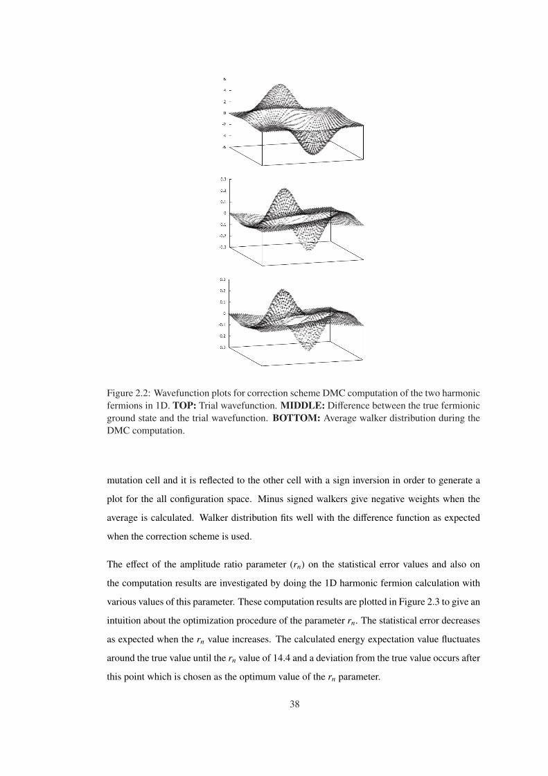
Figure 2.2: Wavefunction plots for correction scheme DMC computation of the two harmonicfermions in 1D. TOP: Trial wavefunction. MIDDLE: Difference between the true fermionicground state and the trial wavefunction. BOTTOM: Average walker distribution during theDMC computation.
mutation cell and it is reflected to the other cell with a sign inversion in order to generate a
plot for the all configuration space. Minus signed walkers give negative weights when the
average is calculated. Walker distribution fits well with the difference function as expected
when the correction scheme is used.
The effect of the amplitude ratio parameter (rn) on the statistical error values and also on
the computation results are investigated by doing the 1D harmonic fermion calculation with
various values of this parameter. These computation results are plotted in Figure 2.3 to give an
intuition about the optimization procedure of the parameter rn. The statistical error decreases
as expected when the rn value increases. The calculated energy expectation value fluctuates
around the true value until the rn value of 14.4 and a deviation from the true value occurs after
this point which is chosen as the optimum value of the rn parameter.
38

0.3458
0.346
0.3462
0.3464
0.3466
0.3468
0.347
0.3472
0.3474
10.3 12.4 14.4 16.5 18.6 20.6
Ecs
rn
Figure 2.3: Calculated energy expectation value versus normalization ratio parameter rn forharmonic fermions in 1D.
Helium atom lowest triplet state
As a physical example, the wavefunction correction technique is used to calculate the non-
relativistic energy expectation value of the lowest triplet state of the Helium atom (1s2s 3S)
without using the fixed-node constraint. This particular state is chosen since it has antisym-
metric spatial wavefunction causing the sign problem. The electronic Hamiltonian function
(Eq. 1.8) is used and the trial wavefunction is chosen as a Slater determinant taken from the
work of Emmanouilidou et al. [81]:
ΨT = e−(2r1+αr2)(1 − α r2) − e−(2r2+αr1)(1 − α r1) , (2.11)
where r1 and r2 are the electron nucleus distances for the two electrons of the system and the
numerical value of the parameter α is chosen as 0.65.
The nodal surface of the studied state of the Helium atom is well known as r1 = r2 surface
[45] which does not match with the nodal surface of the trial wavefunction (Eq. 2.11) used in
39

the calculation. Trial wavefunction cross section is plotted in Figure 2.4 for r1 = 2 r2 surface.
A node crossing is seen in this plot proving that the nodal surface of Eq. 2.11 extends out
of the true nodal surface. Such node crossings always exist for the surfaces r1 = k r2 with
positive k values.
Figure 2.4: He atom 1s2s 3S state trial wavefunction (Eq. 2.11) cross section on r1 = 2 r2surface. Node crossing is seen at r2 = 0.5 a.u.
DMC time step ∆τ is chosen as 0.0005 atomic time units and the data is collected for 80000
time steps after 6000 thermalization steps. Initial number of plus and minus signed walkers
and the number of points for the vacuum branchings are set to 500. The reference energy
adjustment parameter is chosen as 2 × 10⁻⁶. The amplitude of the trial wavefunction is set to
2600 and the number of walkers of each sign is stabilized around 520, giving the rn value as
5.0.
The non-relativistic true energy expectation value for this state is -2.1752 Hartrees [82] and
the energy expectation value of the used trial wavefunction is -2.1548 Hartrees. Current cor-
rection scheme calculation gives the result as -2.1767(63) Hartrees for which the true value
is in the statistical error interval. Same kind of comparison is made for the He atom as in the
case of the harmonic fermions and the computation time of the correction scheme calculation
is 4.2 times shorter than the computation time to achieve the same precision with the compar-
ison case calculation without any trial wavefunctions. Fixed-node DMC calculation using the
nodes of the used trial wavefunction gives the energy value as -2.1626(8) Hartrees confirming
the deviation of the trial wavefunction nodal surface from the true nodal surface r1 = r2.
40

Hydrogen molecule
The last computation used for benchmarking is carried out for the Hydrogen molecule. As in
the case of the helium atom, the lowest lying state with antisymmetric spatial wavefunction
is studied. In fact, this state of the Hydrogen molecule is not a bound state since there is a
repulsive force between the two nuclei for all separation distances d. However, a single point
energy calculation can still be carried out for a chosen separation of the nuclei which was
chosen as d = 3.0 a.u. in the current calculation.
The trial wavefunction is chosen as a Slater determinant formed by the hydrogenic ground
state orbitals around the two nuclei:
ΨT = e−(r11+r22)/d − e−(r12+r21)/d , (2.12)
where ri j denote distances between ith electron and jth nucleus. The energy expectation value
of this trial wavefunction is calculated as −0.9646 Hartrees using Monte Carlo integration
technique. ∆τ, thermalization steps and data collection steps parameter values are chosen
as the same values as the He atom calculation case. Initial number of walkers from each
sign (N+,N−) and the parameter Nvb are set to 400. ΨT amplitude is set to 2000 and the
population sizes are stabilized around 437 giving an rn value of 4.6. The energy expectation
value for the studied state is calculated as −0.9699(38) Hartrees using the non fixed-node
correction scheme DMC which is slightly lower than the trial wavefunction energy. The
computation time is roughly 33 minutes which is 3.5 times shorter than the computation using
the non fixed-node calculation without wavefunction correction technique to achieve the same
precision.
2.2.5 Discussion about the benchmark calculation results
Application of the wavefunction correction scheme to the non fixed-node DMC reduces the
statistical error of the method significantly. Benchmark computations on the harmonic fermions,
helium atom and the hydrogen molecule show that the computation time for calculating the re-
sult within a certain statistical error value decreases several times when the correction scheme
is used. Improvement of the precision depends on the ratio of the trial wavefunction ampli-
41
tude to the number of walkers and this parameter of the method can be increased when the
trial wavefunction gets closer to the true fermionic wavefunction. Therefore, quality of the
trial wavefunction is an important factor affecting the precision improvements observed in
the correction scheme calculations. The mentioned ratio parameter value should be set to the
highest value allowing a full correction which can be guessed considering the quality of the
trial wavefunction. This parameter value can be optimized using the fact that a deviation in
the calculated expectation value starts to occur beyond the optimum value of the parameter.
The nodal surfaces of the used trial wavefunctions deviate from the true surfaces for the all
cases except the harmonic fermions calculation in 1D for which a permutation cell preserv-
ing node distortion is not possible. The correction scheme calculations yield the true energy
expectation value despite the wrong nodal surfaces which proves the applicability of the wave-
function correction scheme for the non fixed-node QMC calculations. This discussion does
not apply to the hydrogen molecule calculation for which the true value of the calculated state
is not available.
The fixed-node DMC is applicable to large systems since it eliminates the minus signed walk-
ers by constraining the computation in a nodal region. This advantage of the fixed-node ap-
proximation disappears with the usage of the correction scheme because of the arising minus
signed walkers as a result of the vacuum branchings. However, the wavefunction correction
technique is suitable for non fixed-node DMC computations since the minus signed walk-
ers are already needed for plus-minus cancellation methods. Correction scheme improves
the large scale applicability for such calculations as opposed to the case for the fixed-node
calculations.
Benchmark computations are carried out without using the importance sampling transforma-
tion in order to better observe the sole effect of the wavefunction correction technique. Im-
portance sampling may be facilitated in the correction scheme calculations as described in the
references [78, 79]. However, the guiding function should allow the walkers’ passage from
the boundaries of the chosen permutation cell for the application of the current boundary con-
ditions when the fixed-node constraint is relaxed. A slightly modified form of the corrected
trial wavefunction which does not vanish on the nodal surface of the original function may be
used as the guiding function.
42

2.3 Stable Non Fixed-Node Algorithm Using Correction Scheme
Some modifications on the wavefunction correction scheme are discussed in this section to-
wards the development of a DMC algorithm which does not suffer from the instabilities due to
the fermion sign problem. These developments do not resolve the sign problem but they serve
as a different viewpoint towards the solution and understanding the nature of the problem.
2.3.1 Downwards shift of the trial wavefunction
In the original form of the wavefunction correction scheme, the trial wavefunction is cor-
rected both in the positive and negative directions depending on the sign of the difference
ΨGS (x) − ΨT (x). Therefore, minus signed walkers are indispensable for the correction pro-
cess in the negative direction. Negative directional corrections can be avoided by a certain
amount downwards shifting of the trial wavefunction ΨT (x) which is illustrated in Figure 2.5.
Figure 2.5: Downwards shift of the trial wavefunction ΨT (x). Dashed Line: Shifted trialwavefunction Ψs
T (x), Solid Line: Ground state wavefunction ΨGS (x), Dotted Line: Differ-ence function ΨGS (x) − Ψs
T (x).
The difference function ΨGS (x) − ΨsT (x) becomes positive definite as seen in the figure if the
shift amount is sufficient. Necessary shift amount for having a positive definite difference
function reduces as the quality of the trial wavefunction increases.
The shifting of the trial wavefunction may be position dependent using a shift function S (x):
ΨsT (x) = ΨT (x) − S (x) . (2.13)
43
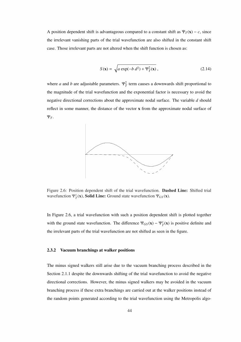
A position dependent shift is advantageous compared to a constant shift as ΨT (x) − c, since
the irrelevant vanishing parts of the trial wavefunction are also shifted in the constant shift
case. Those irrelevant parts are not altered when the shift function is chosen as:
S (x) =
√a exp(−b d2) + Ψ2
T (x) , (2.14)
where a and b are adjustable parameters. Ψ2T term causes a downwards shift proportional to
the magnitude of the trial wavefunction and the exponential factor is necessary to avoid the
negative directional corrections about the approximate nodal surface. The variable d should
reflect in some manner, the distance of the vector x from the approximate nodal surface of
ΨT .
Figure 2.6: Position dependent shift of the trial wavefunction. Dashed Line: Shifted trialwavefunction Ψs
T (x), Solid Line: Ground state wavefunction ΨGS (x).
In Figure 2.6, a trial wavefunction with such a position dependent shift is plotted together
with the ground state wavefunction. The difference ΨGS (x) − ΨsT (x) is positive definite and
the irrelevant parts of the trial wavefunction are not shifted as seen in the figure.
2.3.2 Vacuum branchings at walker positions
The minus signed walkers still arise due to the vacuum branching process described in the
Section 2.1.1 despite the downwards shifting of the trial wavefunction to avoid the negative
directional corrections. However, the minus signed walkers may be avoided in the vacuum
branching process if these extra branchings are carried out at the walker positions instead of
the random points generated according to the trial wavefunction using the Metropolis algo-
44

rithm. Instead of creating a minus signed walker, the walker on which the extra branching is
being made is killed in this case. The branching factors for such an application are calculated
as:
W(x) = 1 − [EL(x) − ER]∆τ ΨsT (x)/Dw(x, τ) . (2.15)
The rescaling factor ΨsT (x)/Dw(x, τ) is necessary since the extra branchings are carried out ac-
cording to a distribution other than the trial wavefunction ΨsT (x). The division factor Dw(x, τ)
is the instantaneous value of the walker distribution at the position of the branching which can
be calculated as a density of walkers calculation at the close neighborhood of the branching
position. The density of walkers calculation is carried out as counting the walkers in a cer-
tain cubical box having the same dimensionality as the configuration space, centered at the
branching position. This density measure works very well for small dimensional configura-
tion spaces and it enables the vacuum branchings to be carried out without any need for the
minus signed walkers. However, as the dimensionality of the configuration space increases,
the dimensions of the box in which the walkers are counted should also increase in order to
have a non vanishing probability of some walkers being counted in the box. For relatively
large systems, the dimensions of the box becomes comparable to the dimensions of the rel-
evant configuration space where the physical wavefunction has significantly non zero values
and the density measure consequently becomes imprecise. For better describing the problem
about the mentioned density measure, the formula for the length of a dimension of the chosen
box (lbox) is given below to have a volume which is 1/1000 of the volume of the relevant
configuration space which is assumed to be box shaped for convenience:
lbox =l
d×n√1000, (2.16)
where l is the length of a dimension of the relevant configuration space. As an example, the
numerical value of the ratio lbox/l becomes 0.9332 when the configuration space dimension
(d × n) is 100.
An alternative density calculation technique, which would better work for higher dimensional
configuration spaces, is to use the average distance between certain number of walkers in
the close neighborhood of the branching position. However, tests with such a density mea-
45
sure shows that it does not give results with sufficient precision even for small systems and
therefore not suitable.
The mentioned problem about the density measure is indeed originated from the fact that the
walker distribution becomes very sparse as the dimensionality of the configuration space in-
creases. The sparsity of the walker distribution, therefore, avoids the large scale applicability
of the stable method described in this section.
2.3.3 Two permutation cells and two reference energies
A technique to avoid the minus signed walkers in the vacuum branching process was dis-
cussed in the previous subsection. However, the minus signed walkers arise also due to the
sign inversions at the permutation cell boundaries as described in Section 1.3.5. These sign
inversions are avoided by making the calculation in two permutation cells (instead of a sin-
gle permutation cell) related to each other with a single permutation of identical particles (or
any odd numbered permutations). When such a simulation region is chosen, all the outgoing
walkers are taken inside by the appropriate particle permutations without any sign inversions.
However, the antisymmetry condition of the fermionic wavefunction in this case should be
imposed in a different manner since the avoided process of sign inversions at the permuta-
tion cell boundaries had previously served for the antisymmetry imposition in the method
described in Section 2.2.
The antisymmetry is imposed in the two permutation cells calculation by normalizing the
wavefunction separately in the two cells using two reference energies. The sums∫
ΨsT (x) dΩ1+
N1 and∫
ΨsT (x) dΩ2 + N2 are kept constant at different values (The normalization value in
the second cell is the multiplication inverse of the normalization value in the first cell as re-
quired by the antisymmetry.) in the two cells via adjustments of the reference energies E1R, E2
R
separately. N1 and N2 in the above expressions denote the number of walkers in the first and
second cells respectively. These walkers have all plus signs since the minus signed walkers
are avoided with the techniques described in the previous and current subsections.
Using two separate reference energies in the two cells corresponds to introducing a position
dependent reference energy ER(x) in Eq. 1.16. Therefore, the stable method described in
this section is not exact even if an accurate density measure could have been devised for
46
the application of the vacuum branchings at walker positions as described in the previous
subsection.
2.3.4 Harmonic fermion calculations using the stable algorithm
The stable DMC algorithm described in previous subsections is used to calculate the ground
state eigenvalues of the harmonic fermions discussed in Section 2.2.4. The purpose of these
calculations is to test the effects of the density measure and the usage of two reference energies
on the accuracy of the results. Trial wavefunction given in Eq. 2.10 is used as ΨT also in
these calculations. ΨsT is generated according to the formula given in Eq. 2.13 using the shift
function S (x) of Eq. 2.14.
The calculation is initially carried out for one space dimension to test the effect of two ref-
erence energy usage. The density measure as counting the walkers in a certain cubical box
is accurate enough for such a small dimensional system and thus the sole effect of the two
reference energies is tested with this 1D calculation. The disturbance parameters ε1 and ε2
of the trial wavefunction (Eq. 2.10) are given the values 0.9238 and 0.0 respectively. The
parameters a and b of the shift function S (x) are set to the values 1.0 and 0.1 respectively.
The distance d in S (x) expression is measured from the origin of the coordinate system. ∆τ is
set to 0.001 and α is set to 0.00001. The numbers of walkers in each cell is kept constant at
500 and the values of∫
ΨsT (x) dΩ integrals are given the values −83.6 and −916.4 in the two
cells to satisfy the antisymmetry condition of the wavefunction. The length of a dimension of
the cubical box is set to 0.77 dimensionless units (d.u.) for the density of walkers calculation.
The ground state energy eignvalue is calculated as 0.3465(11) d.u. using the stable correction
scheme DMC algorithm with shifted trial wavefunction in 280000 time steps. The calculated
value is very close to the true value which is 0.34641 d.u. for the 1D harmonic fermions (see
Table 2.1). The values of the two reference energies deviate from each other significantly
during the computation. However, the time averages of them are 0.34892 and 0.35179 d.u.
for E1R and E2
R which are close to each other. Therefore, two reference energy usage does not
cause a significant bias for the 1D calculation. Average walker distribution during this com-
putation is compared with the expected walker distribution (ΨGS − ΨsT ) in Figure 2.7. The
comparison shows that the shape of the walker distribution fits with the expected distribution
in general. However, it is not as accurate as the calculation results of Section 2.2 which was
47
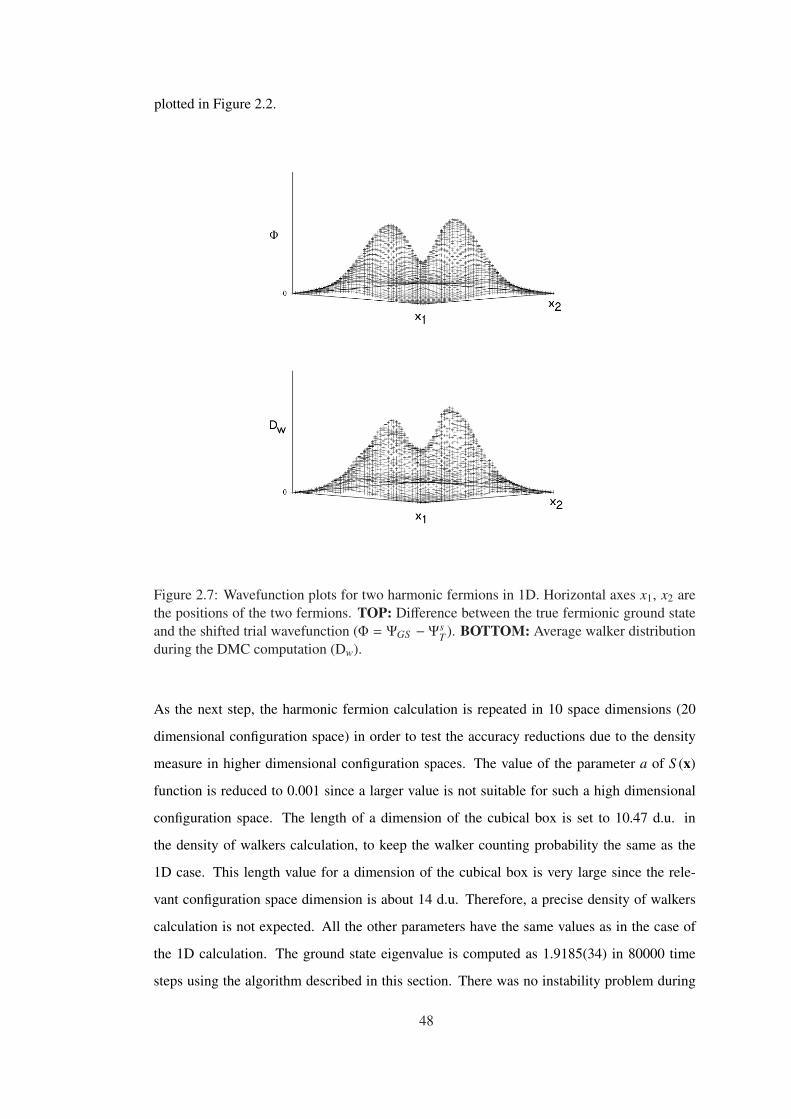
plotted in Figure 2.2.
Figure 2.7: Wavefunction plots for two harmonic fermions in 1D. Horizontal axes x1, x2 arethe positions of the two fermions. TOP: Difference between the true fermionic ground stateand the shifted trial wavefunction (Φ = ΨGS − Ψs
T ). BOTTOM: Average walker distributionduring the DMC computation (Dw).
As the next step, the harmonic fermion calculation is repeated in 10 space dimensions (20
dimensional configuration space) in order to test the accuracy reductions due to the density
measure in higher dimensional configuration spaces. The value of the parameter a of S (x)
function is reduced to 0.001 since a larger value is not suitable for such a high dimensional
configuration space. The length of a dimension of the cubical box is set to 10.47 d.u. in
the density of walkers calculation, to keep the walker counting probability the same as the
1D case. This length value for a dimension of the cubical box is very large since the rele-
vant configuration space dimension is about 14 d.u. Therefore, a precise density of walkers
calculation is not expected. All the other parameters have the same values as in the case of
the 1D calculation. The ground state eigenvalue is computed as 1.9185(34) in 80000 time
steps using the algorithm described in this section. There was no instability problem during
48

the calculation of this higher dimensional system. However, the accuracy of the result is not
very good since it deviates from the true value which is 1.9053 for the studied two harmonic
fermions in 10D. This bias in the calculated result is expected since the density measure was
very imprecise for this higher dimensional calculation.
49

CHAPTER 3
CONCLUSIONS
Some developments on the DMC method, which is used to find the ground state solutions of
the Schrodinger equation, are discussed in this thesis work. The context of the developments is
divided in to two parts both related to the wavefunction correction scheme DMC calculations:
The first part of the developments (Section 2.2) are about the application of the wavefunction
correction scheme to the non fixed-node DMC in order to reduce the statistical error bars
obtained in a certain amount of computation time. The non fixed-node DMC method used
in the calculations does not have the nodal systematic error encountered in the fixed-node
DMC calculations. However, it is unstable due to the fermion sign problem and consequently
its application to relatively large systems is not possible. The developments of the first part
does not affect the stability of the non fixed-node DMC but they are aimed to shorten the
computation times of the non fixed-node calculations in their current application range. The
benchmark computation results indicate that computation times to achieve a certain precision
decreases several times when the correction scheme is used in the non fixed-node DMC.
Therefore, the objective of the developments of the first part is achieved successfully. Also, it
should be noted that, the wavefunction correction technique introduces minus signed walkers
to the boson and fixed-node fermion calculations and thus it reduces the stability of such DMC
calculations. This problem does not arise in the non fixed-node DMC framework since the
minus signed walkers and the instability are already inherit in such calculations.
In the second part of the developments, discussed in Section 2.3, some modifications on the
original wavefunction correction scheme are studied with a purpose of having a stable non
fixed-node DMC algorithm. These developments avoid the minus signed walkers in such
calculations by converting the plus - minus cancellation process in to a density of walkers
50

calculation. Both of these processes suffer from the sparsity of the walker population in
higher dimensional configuration spaces when relatively larger systems are considered. The
necessity for the density of walkers calculation in the new developments reduces the accuracy
of the DMC calculations, especially for large systems, since an accurate density calculation
is not possible for a very sparse walker distribution. However, the developed method is stable
and it is useful for understanding the nature of the fermion sign problem. Since a sparse walker
distribution is the main cause of the problem in the new developed method as in the case of
the plus - minus cancellation methods, it becomes apparent that an exact fermion calculation
is not possible in the DMC framework without fully generating the wavefunction. In other
words, the statistical sampling techniques, which are very successful for boson calculations,
become inefficient when the antisymmetry condition of the fermions is desired to be imposed
on the wavefunction exactly.
51

REFERENCES
[1] K. Raghavachari. Electron correlation techniques in quantum chemistry: Recent ad-vances. Annu. Rev. Phys. Chem., 42:615–42, 1991.
[2] R. J. Bartlett and M. Musia. Coupled-cluster theory in quantum chemistry. Rev. Mod.Phys., 79:291–352, 2007.
[3] S. Goedecker. Linear scaling electronic structure methods. Rev. Mod. Phys., 71:1085–1123, 1999.
[4] G. E. Scuseria. Linear scaling density functional calculations with gaussian orbitals. J.Phys. Chem. A, 103:4782–4790, 1999.
[5] P. Hohenberg and W. Kohn. Inhomogeneous electron gas. Phys. Rev., 136:B864–B871,1964.
[6] M. Springborg. Methods of Electronic-Structure Calculations. John Wiley and SonsLtd., 2000.
[7] W. A. Lester A. Aspuru-Guzik. Quantum Monte Carlo methods for the solution of theSchrodinger equation for molecular systems. arXiv: cond-mat, 0204486, 2002.
[8] W. M. C. Foulkes, L. Mitas, R. J. Needs, and G. Rajagopal. Quantum Monte Carlosimulations of solids. Rev. Mod. Phys., 73:33–83, 2001.
[9] P. Echenique and J. L. Alonso. A mathematical and computational review of Hartree-Fock SCF methods in quantum chemistry. Molecular Physics, 105:3057–3098, 2007.
[10] J. B. Anderson. Quantum chemistry by random walk. H+3 D3h
1A1, H23 ∑+
u , H41 ∑+
g ,Be 1S . J. Chem. Phys, 65:4121–4127, 1976.
[11] R. Shankar. Principles of Quantum Mechanics, 2nd Edition. Plenum Press, New York,1994.
[12] J. J. Sakurai. Modern Quantum Mechanics, Rev. ed. Addison Wesley, 1994.
[13] E. Schrodinger. Quantisierung als eigenwertproblem. Annalen der Physik. Leipzig,79:489–527, 1926.
[14] H. P. Stapp. The Copenhagen interpretation. Am. J. Phys., 40:1098–1116, 1972.
[15] A. Whitaker. Einstein, Bohr and the quantum dilemma. Cambridge University Press,New york, 1996.
[16] J. D. Walecka. Fundamentals of Statistical Mechanics. Imperial College Press, WorldScientific, Singapore, 2000.
[17] I. Duck and E. C. G. Sudarshan. Toward an understanding of the spin-statistics theorem.Am. J. Phys., 66:284–303, 1998.
52

[18] H. C. Ohanian. What is spin. Am. J. Phys., 54:500–505, 1986.
[19] M. Born and R. Oppenheimer. Zur quantentheorie der molekule. Annalen der Physik.Leipzig, 84:457–484, 1927.
[20] A. J. James. Solving the Many Electron Problem with Quantum Monte-Carlo Methods.PhD thesis, Imperial College of Science, 1995.
[21] I. Kosztin, B. Faber, and K. Schulten. Introduction to the diffusion Monte Carlo method.Am. J. Phys., 64:633–646, 1996.
[22] N. Metropolis. The beginning of the Monte Carlo method. Los Alamos Science, SpecialIssue:125–130, 1987.
[23] W. A. Lester, L. Mitas, and B. Hammond. Quantum Monte Carlo for atoms, moleculesand solids. Chem. Phys. Lett., 478:1–10, 2009.
[24] R. J. Needs, M. D. Towler, N. D. Drummond, and P. L. Rios. Continuum variational anddiffusion quantum Monte Carlo calculations. J. Phys.: Condens. Matter, 22:023201–15,2010.
[25] H. G. Evertz and M. Marcu. Quantum Monte Carlo methods in condensed matterphysics, ed. M. Suzuki. World Scientific, Singapore, 1993.
[26] J. Shumway and D. M. Ceperley. Quantum Monte Carlo Methods in the Study of Nanos-tructures in Handbook of Theoretical and Computational Nanotechnology ,eds. M. Riethand W. Schommers, Encyclopedia of Nanoscience and Nanotechnology, Vol. 3. Ameri-can Scientific Publishers, 2006.
[27] J. B. Anderson. Quantum Monte Carlo: Origins, Development, Applications. OxfordUniversity Press, New york, 2007.
[28] R. N. Barnett and K. B. Whaley. Variational and diffusion Monte Carlo techniques forquantum clusters. Phys. Rev. A, 47:4082–4098, 1993.
[29] S. A. Alexander and R. L. Coldwell. Calculating atomic properties using variationalMonte Carlo. J. Chem. Phys., 103:2572–2575, 1995.
[30] N. A. Benedek, I. K. Snooka, M. D. Towler, and R. J. Needs. Quantum Monte Carlocalculations of the dissociation energy of the water dimer. J. Chem. Phys., 125:104302–5, 2006.
[31] M. H. Kalos. Monte Carlo calculations of the ground state of three- and four-bodynuclei. Phys. Rev., 128:1791–1795, 1962.
[32] D. M. Ceperley. Metropolis methods for quantum Monte Carlo simulations.arXiv:physics, 0306182, 2003.
[33] M. Lewerenz. Monte Carlo methods: Overview and basics. NIC Series, 10:1–24, 2002.
[34] R. H. Landau, M. J. Paez, and C. C. Bordeianu. Computational Physics: ProblemSolving with Computers. WILEY-VCH, 2007.
[35] N. Metropolis, A. Rosenbluth, M. Rosenbluth, A. Teller, and E. Teller. Equation of statecalculations by fast computing machines. J. Chem. Phys., 21:1087–000, 1953.
53

[36] E. Polak. Optimization : Algorithms and Consistent Approximations. Springer, NewYork, 1997.
[37] P. Ballone and P. Milani. Simulated annealing of carbon clusters. Phys. Rev. B, 42:3201–3204, 1990.
[38] S. Forrest. Genetic algorithms: Principles of natural selection applied to computation.Science, 261:872–878, 1993.
[39] J. C. Slater. Theory of complex spectra. Phys. Rev., 34:293–1322, 1929.
[40] D. Ceperley. Solving quantum many-body problems with random walks. ComputationalPhysics, Proceedings of Ninth Physics Summer School, Australian National University,1997.
[41] G Ortiz, D. M. Ceperley, and R. M. Martin. New stochastic method for systems withbroken time-reversal symmetry; 2-D fermions in a magnetic field. Phys. Rev. Lett.,71:2777–0000, 1993.
[42] R.C. Grimm and R.G. Storer. Monte Carlo solution of Schrodinger’s equation. J. Com-put. Phys., 7:134–156, 1971.
[43] R. Assaraf, M. Caffarel, and A. Khelif. The fermion Monte Carlo revisited. J. Phys. A:Math. Theor., 40:1181–1214, 2007.
[44] M. Troyer and U. J. Wiese. Computational complexity and fundamental limitationsto fermionic quantum Monte Carlo simulations. Phys. Rev. Lett., 94:170201–170204,2005.
[45] D. Bressanini, D. M. Ceperley, and P. J. Reynolds. What do we know about wavefunction nodes? arXiv:quant-ph, 0106062, 2001.
[46] M. Bajdich, L. Mitas, G. Drobny, and L. K. Wagner. Approximate and exact nodesof fermionic wavefunctions: Coordinate transformations and topologies. Phys. Rev. B,72:075131–5, 2005.
[47] S. Manten and A. Luchow. On the accuracy of the fixed-node diffusion quantum MonteCarlo method. J. Chem. Phys., 115:5362–5366, 2001.
[48] J. C. Grossman and L. Mitas. Quantum Monte Carlo determination of electronic andstructural properties of Sin clusters (n ≤ 20). Phys. Rev. Lett., 74:1323–1326, 1995.
[49] W. A. Lester and R. Salomon-Ferrer. Some recent developments in quantum MonteCarlo for electronic structure: Methods and application to a bio system. J. Mol. Struct.:THEOCHEM, 771:51–54, 2006.
[50] E. Sola, J. P. Brodholt, and D. Alfe. Equation of state of hexagonal closed packed ironunder earths core conditions from quantum Monte Carlo calculations. Phys. Rev. B,79:024127–6, 2009.
[51] S. Bovino, E. Coccia, E. Bodo, D. Lopez-Duran, and F. A. Gianturcoa. Spin-drivenstructural effects in alkali doped 4He clusters from quantum calculations. J. Chem.Phys., 130:224903–9, 2009.
54

[52] G. Rajagopal, R. J. Needs, A. James, S. D. Kenny, and W. M. C. Foulkes. Variationaland diffusion quantum Monte Carlo calculations at nonzero wave vectors: Theory andapplication to diamond-structure germanium. Phys. Rev. B, 51:10591–10600, 1994.
[53] R. J. Needs, M. D. Towler, N. D. Drummond, and P. L. Rios. CASINO version 2.3 UserManual. University of Cambridge, 2008.
[54] A. Aspuru-Guzik, R. Salomon-Ferrer, B. Austin, R. Perusquia-Flores, M. A. Griffin,R. A. Olivia, D. Skinner, D. Domin, and W. A. Lester. Zori 1.0: A parallel quantumMonte Carlo electronic structure package. J. Comput. Chem., 26:856–862, 2005.
[55] D. M. Ceperley and L. Mitas. Quantum Monte Carlo methods in chemistry. Adv. Chem.Phys., 93:1–0, 1996.
[56] D. M. Amow, M. H. Kalos, M. A. Lee, and K. E. Schmidt. Green’s function MonteCarlo for few fermion problems. J. Chem. Phys., 77:5562–0000, 1982.
[57] D. M. Ceperley and B. J. Alder. Ground state of the electron gas by a stochastic method.Phys. Rev. Lett., 45:566–569, 1980.
[58] D. M. Ceperley and B. J. Alder. Quantum Monte Carlo for molecules: Green’s functionand nodal release. J. Chem. Phys., 81:5833–4844, 1984.
[59] M. Caffarel and D. M. Ceperley. A bayesian analysis of Green’s function Monte Carlocorrelation functions. J. Chem. Phys., 97:8415–8423, 1992.
[60] Y. Kwon, D. M. Ceperley, and R. M. Martin. Quantum Monte Carlo calculation of thefermi liquid parameters in the two-dimensional electron gas. Phys. Rev. B, 50:1684–1694, 1994.
[61] Y. Kwon, D. M. Ceperley, and R. M. Martin. Transient-estimate Monte Carlo in thetwo-dimensional electron gas. Phys. Rev. B, 53:7376–7382, 1996.
[62] B. Chen and J. B. Anderson. A simplified released-node quantum Monte Carlo calcula-tion of the ground state of LiH. J. Chem. Phys., 102:4491–4494, 1995.
[63] J. B. Anderson, C. A. Traynor, and B. M. Boghosian. Quantum chemistry by randomwalk: Exact treatment of many-electron systems. J. Chem. Phys., 95:7418–7425, 1991.
[64] D. L. Diedrich and J. B. Anderson. An Accurate quantum Monte Carlo calculation ofthe barrier height for the reaction H + H2 → H2 + H. Science, 258:786–788, 1992.
[65] R. Bianchi, D. Bressanini, P. Cremaschi, and G. Morosi. Antisymmetry in quantumMonte Carlo methods. Comput. Phys. Commun., 74:153–163, 1993.
[66] Z. Liu, S. Zhang, and M. H. Kalos. Model fermion Monte Carlo method with antitheticalpairs. Phys. Rev. E, 50:3220–3229, 1994.
[67] M. H. Kalos and F. Pederiva. Exact Monte Carlo method for continuum fermion sys-tems. Phys. Rev. Lett., 85:3547–3551, 2000.
[68] F. Luczak, F. Brosens, J. T. Devreese, and L. F. Lemmens. Many-body diffusion algo-rithm for interacting harmonic fermions. Phys. Rev. E, 57:2411–2418, 1998.
[69] D. M. Ceperley. Fermion nodes. J. Stat. Phys., 63:1237–1266, 1991.
55
[70] R. Bianchi, D. Bressanini, P. Cremaschi, and G. Morosi. Antisymmetry in quantumMonte Carlo method with A-function technique: H2 b 3Σ+
u , H2 c 3Πu, He 1 3S. J. Chem.Phys., 98:7204–7209, 1993.
[71] Y. Mishchenko. Remedy for the fermion sign problem in the diffusion MonteCarlo method for few fermions with antisymmetric diffusion process. Phys. Rev. E,73:026706–10, 2006.
[72] A. J. W. Thom and A. Alavi. A combinatorial approach to the electron correlationproblem. J. Chem. Phys., 123:204106–13, 2005.
[73] S. B. Fahy and D. R. Hamann. Positive-projection Monte Carlo simulation: A newvariational approach to strongly interacting fermion systems. Phys. Rev. Lett., 65:3437–3440, 1990.
[74] P.L. Silvestrelli, S. Baroni, and R. Car. Auxiliary-field quantum Monte Carlo calcula-tions for systems with long-range repulsive interactions. Phys. Rev. Lett., 71:1148–1151,1993.
[75] F. A. Reboredo, R. Q. Hood, and P. R. C. Kent. Self-healing diffusion quantum MonteCarlo algorithms: Direct reduction of the fermion sign error in electronic structure cal-culations. Phys. Rev. B, 79:195117–15, 2009.
[76] J. C. Slater. Note on the space part of anti-symmetric wave functions in the many-electron problem. Int. J. Quantum Chem., 4:561–570, 1970.
[77] J. B. Anderson and B. H. Freihaut. Quantum chemistry by random walk: Method ofsuccessive corrections. J. Comput. Phys, 31:425–437, 1979.
[78] J. B. Anderson. Quantum chemistry by random walk: Higher accuracy. J. Chem. Phys.,73:3897–3899, 1980.
[79] J. B. Anderson. Quantum monte carlo: Direct calculation of corrections to trial wavefunctions and their energies. J. Chem. Phys., 112:9699–9702, 2000.
[80] N. Dugan, I. Kanik, and S. Erkoc. Wavefunction correction scheme for non fixed-nodediffusion Monte Carlo. (submitted).
[81] A. Emmanouilidou, T. Schneider, and J.-M. Rost. Quasiclassical double photoionizationfrom the 21,3S states of helium including shakeoff. J. Phys. B: At. Mol. Opt. Phys.,36:2717–2724, 2003.
[82] D. H. Bailey and A. M. Frolov. Universal variational expansion for high-precisionbound-state calculations in three-body systems. applications to weakly bound, adiabaticand two-shell cluster systems. J. Phys. B: At. Mol. Opt. Phys., 35:4287–4298, 2002.
56

APPENDIX A
PROOF OF THE VARIATIONAL PRINCIPLE
The variational principle which states that the expectation value of an observable O, repre-
sented by a linear and Hermitian operator, is larger than or equal to the ground state eigenvalue
a0:
〈O〉 =〈Ψ(x)|O |Ψ(x)〉〈Ψ(x)|Ψ(x)〉 ≥ a0 , (A.1)
can be proven using the eigenfunction decomposition of the arbitrary state Ψ(x) as:
Ψ(x) =∑
i
ci fi(x) , (A.2)
where fi(x) are the orthanormal eigenfunctions of O and ci are the overlap coefficients defined
as:
ci = 〈 fi(x) | Ψ(x)〉 . (A.3)
Substituting the Ψ(x) expression given in Eq. A.2 in Eq. A.1 gives:
〈O〉 =〈∑i ci fi(x)|O |∑ j c j f j(x))〉〈∑i ci fi(x)|∑ j c j f j(x))〉 . (A.4)
Using the eigenvalue equation O fi(x) = ai fi(x) and the linearity, Eq. A.4 becomes:
〈O〉 =〈∑i ci fi(x)|∑ j c j a j f j(x))〉〈∑i ci fi(x)|∑ j c j f j(x))〉 . (A.5)
57

The orthanormality of the eigenfunctions is used to convert the above expression into the
simple form:
〈O〉 =
∑i, j c∗i c j a j δi j∑
i, j c∗i c j δi j=
∑i c∗i ci ai∑
i c∗i ci=
∑i |ci|2 ai∑
i |ci|2. (A.6)
Using the fact that the eigenvalues ai are greater than or equal to the ground state eigenvalue
a0, the above equality is converted to an inequality:
〈O〉 ≥∑
i |ci|2 a0∑i |ci|2
. (A.7)
The constant a0 can be taken out of the sum, yielding:
〈O〉 ≥ a0∑
i |ci|2∑i |ci|2
= a0 , (A.8)
which proves Eq. A.1.
58

CURRICULUM VITAE
Surname : Dugan
Name : Nazım
Nationality : T.C.
Email : [email protected]
Phone : +90 312 210 4307
EDUCATION
Ph.D in Physics, 2006 : 2010, Middle East Technical University
Supervisor: Sakir Erkoc
Thesis Title: Quantum Monte Carlo Methods for Fermionic Systems: Beyond the Fixed-Node
Approximation.
MS in Physics, 2005 : 2006, Middle East Technical University
Supervisor: Sakir Erkoc
Thesis Title: Structural Properties of Homonuclear and Heteronuclear Atomic Clusters: Monte
Carlo Simulation Study
Ph.D Program in Physics, 2002 : 2004, University of New Hampshire (not completed)
BSc in Physics, 1997 : 2002, Bogazici University
EMPLOYMENT
2007 : ongoing, Middle East Technical University
Assistantship in Physics Department, Computer coordinator of the department
2006 : 2007, Middle East Technical University
Teaching Assistantship
59

2002 : 2004, University of New Hampshire
Teaching Assistantship
Research Assistantship in Computational Space Science Group
2002, Bogazici University
Student Assistantship in Physics Department
PUBLICATIONS
N. Dugan, I. Kanik, S. Erkoc, Wavefunction correction scheme for non fixed-node diffusion
Monte Carlo, arXiv: comp-ph 09123401 (submitted)
N. Dugan, S. Erkoc, Genetic Algorithms in Application to the Geometry Optimization of
Nanoparticles, Algorithms 2, 410 (2009) (Invited review)
N. Dugan, S. Erkoc, Genetic Algorithm Application to the Structural Properties of Si-Ge
Mixed Clusters, Materials and Manufacturing Processes 24, 250 (2009)
N Dugan, S. Erkoc, Genetic algorithm-Monte Carlo hybrid method for geometry optimization
of atomic clusters, Computational Materials Science 45, 127 (2009)
N. Dugan, S. Erkoc, Stability analysis of graphene nanoribbons by molecular dynamics sim-
ulations, Phys. Stat. Sol. (b) 245, 695 (2008)
N. Dugan, S. Erkoc, Structural properties of lithium clusters: A Monte Carlo application, J.
Comput. Meth. Sci. Eng. 7, 409 (2007)
N. Dugan, S. Erkoc, Monte Carlo geometry optimization of Sin (n ≤ 71) clusters, J. Comput.
Meth. Sci. Eng. 7, 233 (2007)
N. Dugan, S. Erkoc, Geometry Optimization of ZnnCdm and (AlTiNi)n Clusters by the Modi-
fied Diffusion Monte Carlo Method, Comput. Lett. 2, 221 (2006)
N. Dugan, S. Erkoc, Structural Properties of Copper Nanoparticles: Modified Diffusion
Monte Carlo Simulations, Int. J. Mod. Phys. C 17, 1171 (2006)
60

ATTENDED CONFERENCES AND SUMMER SCHOOLS
13th International Congress on Quantum Chemistry, Helsinki Finland, 2009
Poster: Wavefunction Shift Technique for Exact Diffusion Monte Carlo Computations
14th International Workshop on Computational Physics and Materials Science, Trieste Italy,
2009, Poster: Shifted Wavefunction Diffusion Monte Carlo for Fermions
Quantum Monte Carlo and the Casino Program (Summer School), Vallico Sotto Italy, 2008,
Student Talk: Fermion Sign Problem in Diffusion Monte Carlo
NanoTR III, Bilkent University Ankara Turkey, 2007, Talk: Genetic algorithm - Monte Carlo
hybrid method for finding stable geometries of atomic clusters
E-MRS Fall Meeting, Warsaw Poland, 2007, Talk: Genetic algorithm-Monte Carlo hybrid
method for geometry optimization of atomic clusters
NANOMAT, Antalya Turkey, 2006 Poster: Application of Diffusion Monte Carlo Method to
Geometry Optimization of Atomic Nanoparticles.
NanoTR II, METU Ankara Turkey, 2006 Poster: Structural Properties of Copper Nanoparti-
cles
61