OPTIMIZATION OF A PRODUCTION LOT SIZING …ijoce.iust.ac.ir/article-1-245-en.pdfOPTIMIZATION OF A PR ODUCTION LOT SIZING PROBLEM WITH QUANTITY DISCOU NT S. Khosravi and S.H. Mirmohammadi*,

INTERNATIONAL JOURNAL OF OPTIMIZATION IN CIVIL ENGINEERING

Int. J. Optim. Civil Eng., 2016; 6(2):187-209

OPTIMIZATION OF A PRODUCTION LOT SIZING PROBLEM

WITH QUANTITY DISCOUNT

S. Khosravi and S.H. Mirmohammadi*, † Department of Industrial and systems Engineering, Isfahan University of Technology,

Isfahan, Iran

ABSTRACT

Dynamic lot sizing problem is one of the significant problem in industrial units and it has

been considered by many researchers. Considering the quantity discount in purchasing cost

is one of the important and practical assumptions in the field of inventory control models

and it has been less focused in terms of stochastic version of dynamic lot sizing problem. In

this paper, stochastic dynamic lot sizing problem with considering the quantity discount is

defined and formulated. Since the considered model is mixed integer non-linear

programming, a piecewise linear approximation is also presented. In order to solve the

mixed integer non-linear programming, a branch and bound algorithm are presented. Each

node in the branch and bound algorithm is also MINLP which is solved based on dynamic

programming framework. In each stage in this dynamic programming algorithm, there is a

sub-problem which can be solved with lagrangian relaxation method. The numeric results

found in this study indicate that the proposed algorithm solve the problem faster than the

mathematical solution using the commercial software GAMS. Moreover, the proposed

algorithm for the two discount levels are also compared with the approximate solution in

mentioned software. The results indicate that our algorithm up to 12 periods not only can

reach to the exact solution, it consumes less time in contrast to the approximate model.

Keywords: dynamic lot sizing problem; total quantity discount; branch and bound

algorithm; dynamic programming; lagrangian relaxation method.

Received: 20 September 2015; Accepted: 8 November 2015

1. INTRODUCTION

One of the major and basic responsibilities in the industrial units is production planning and

*Corresponding author: Department of industrial and systems Engineering, Isfahan University of

Technology, Iran, P.B. BOX: 8415683111 †E-mail address: [email protected]

Dow

nloa

ded

from

ijoc

e.iu

st.a

c.ir

at 1

2:42

IRD

T o

n S

unda

y M

ay 2

0th

2018

http://ijoce.iust.ac.ir/article-1-245-en.html

S. Khosravi and S.H. Mirmohammadi

188

inventory control. The issue of inventorying material and planning for high quality

production with favorable volume at suitable time and reasonable price are of the major

concerns of the managers. Economic order quantity models or lot sizing has been developed

to achieve this goal.

Economic order quantity determines how much and when a special product should be

ordered so that the system costs, which often include holding, ordering and purchasing costs,

are minimized [1]. "Dynamic lot sizing programming" refers to those issues where planning

horizon is limited and discrete, or in better words, is assumed periodically and the demand is

different from one period to another [1]. Many elements affect the variety of lot sizing

models, and by definition, in the area of production planning and inventory control, different

specifications and assumptions are considered for the model. Among these specifications

type of demand, capacity constraints, the number of items, planning horizon and the

purchase cost can be noted.

Discount on good purchase has often been raised in deterministic issues. Callerman and

Whybark [2] presented a Mixed-Integer Programming (MIP) model for ordering problem

with quantity discount through which optimal ordering policy is obtained by binary decision

variables. On the issue of determining deterministic lot sizing and considering discount,

Chung et al. [3] proved that there is an optimal policy that order quantity between any two

consecutive re-ordering points, except for that last order, is equal to one of the discount

levels. Using this feature, an algorithm based on dynamic programming algorithm was

presented that solve the problem more efficiently than Callerman and Whybark's algorithm.

Mirmohammadi et al. [4] presented a branch and bound algorithm for determining the

quantity of orders, in deterministic single item cases while considering discount that is more

efficient in solving large-scale problems (many periods and high discount levels) compared

to previous methods. Goossens et al. [5] demonstrated that there is no polynomial algorithm

to solve multi item lot sizing problem considering total quantity discount. In other words,

this problem known as TQD is in NP-hard class.

There are two approaches to control unfilled demand in stochastic lot sizing models.

Standard approach is introducing the penalty cost for backlogged sales in the objective

function. In some cases, calculating this parameter, if not impossible, is too difficult that

leads to the use of technical performance standards. The second approach is using service

level constraints. The decision makers determine the level of satisfaction with these

standards. In the literature of the issue, various performance standards are considered which

the most important of them are α, β, γ service levels [6].

The first studies in the field of random demand and considering it in lot-sizing problems

was carried out by Silver in 1978 [7]. Silver offered a heuristic three-stage method to

determine lot-size with random demand. Bookbinder and Tan [8] modeled the stochastic lot

sizing problem in a single-stage state with regard to α service level constraint. In order to

control the randomness of demand over time, according to the conditions of inventory and

production systems, three strategies have been identified: dynamic uncertainty strategy,

static-dynamic uncertainty strategy, static uncertainty strategy. They showed that the

mathematical structure of stochastic problem with α service level and static uncertainty

strategy is the equivalent to a deterministic lot-size model and deterministic lot sizing

problem solving methods can be used to solve the stochastic version. Vargas [9] presented

an optimal algorithm for solving the stochastic un-capacitated lot sizing problem. This is

Dow

nloa

ded

from

ijoc

e.iu

st.a

c.ir

at 1

2:42

IRD

T o

n S

unda

y M

ay 2

0th

2018


OPTIMIZATION OF A PRODUCTION LOT SIZING PROBLEM WITH …

189

called as stochastic version of Wagner–Whitin problem. Sox in [10] dealt with optimal

solving of stochastic dynamic lot sizing problem by considering non-stationary purchase

cost. Tempelmeier [11] has reviewed the mathematical models of stochastic lot sizing

problems and developed a model with static-dynamic strategy considering fill rate β in

whose solution inventory on hand is used instead of net inventory. Vargas and Mitters [12]

developed the heuristic PDLA algorithm to solve the stochastic single item un-capacitated

lot sizing problem in single-stage state by considering penalty cost for unfilled demand in a

rolling planning horizon. This algorithm is an extension of optimal algorithm of shortest

path problem in static uncertainty strategy.

Quantity discount has newly been studied in stochastic dynamic lot sizing models and

few articles have been published in this regard. Hajji et al. studied the quantity discount in

single-period model (the newsboy problem) in 2007 with the random initial inventory. For

this problem, the optimum quantity of order is determined to maximize profit and the

problem is rewritten with random demand and inventory variables in normal mode. In Kang

and Lee [14], single item dynamic lot sizing problem with random demand by considering

the total quantity discount in supplier selection field has been investigated, a heuristic

method based on Dynamic Programming (HDP) has also been developed to solve the

problem.

The remainder of the paper has been organized as follows. In Section 2, the problem is

defined and beside two mathematical non-linear models of the problem, a piecewise linear

model of the problem is presented. Section 3 presents the solution approach of the problem

which is based on decomposing the problem in four levels. In each level, a proper approach

is applied to handle the sub-problem of the level. In Section 4 some test problems randomly

generated are solved by two approaches to evaluate their efficiency relatively. Concluding

remarks and results are appeared in Section 5.

2. PROBLEM DEFFINITION AND FORMULATION

In basic models of stochastic dynamic lot sizing problem, it is assumed that the unit price of

the ordered items will not change by the quantity of each order. In this paper, a model is

investigated in which unit item price depends on the quantity of each order. This means that

retailers and product suppliers of commodity offer that if the order quantity x reaches a

certain value q, they are willing to sell total value of x to a price lower than c to the buyer.

At this point, the newly announced price includes the total value of order x. This price

structure is called All-unit discount. This discount cost structure can be defined as non-

stationary for the case that the purchase price is non-stationary. In other words, discounts

policy is different at any period compared with the others (both in term of price and discount

levels). In this study, it is assumed that the number of discount levels K is the same for all

periods, but without this assumption the presented model will still be valid. In the intended

problem, the demand is considered for one item, and the time horizon is finite. Ordering cost

in each period is considered only in case of ordering and resources are unlimited. Demand is

assumed to be random and continuous. Shortage is allowed in form of backlogging and the

amount of shortage is controlled as shortage penalty cost in the objective function. Demand

is random and its density function is known and in any period is independent of other

Dow

nloa

ded

from

ijoc

e.iu

st.a

c.ir

at 1

2:42

IRD

T o

n S

unda

y M

ay 2

0th

2018



190

periods. Shortage, holding and ordering costs can vary from one period to another. The goal

is to minimize the expected cost of holding cost, shortage cost, ordering cost and purchase

cost in total planning horizon. At the beginning of the planning horizon, time and amount of

ordering is determined for the entire planning horizon. In this study, the issue Stochastic

Single item Discounted Lot Sizing Problem is expressed as with the abbreviation SSDLSP.

2.1. Mixed integer nonlinear modes

In this section we formulated the problem in two different ways which lead to two different

mixed integer nonlinear models. The following notation is used in the mathematical

formulation of the problem:

T Number of periods in planning horizen

K Number or discount level

and for period t , Tt ,...,2,1 ,

tA Ordering cost th Holding cost

t Backorder penalty cost

M A sufficeintly large nublmer

tD Demand

tx Ordering quantity

tX Cumulative order quantity through periods 0 to t )(

1

t

j

jt xX

tY Cumulative demand through period0 to t (

t

j

jt DY

1

)

)( tY yft

p.d.f of tY )( tY yF

t c.d.f of tY

)( tt XL Total expected holding and penalty costs incurred at the end of period t ts A binary variable which is 1 if an ordering occuredin period t, 0 otherwise tkq The minimum acceptable quantity to deserve for discount level k in period t

tkc Unit Purchasing cost in period t and in discount level k

tku A binary variable which is 1 if an order performed in period t in discount level k ,

0 otherwise

The problem can be formulated as follows.

)()(}{ 1

1

tttttt

T

t

t XXcXLsAcEMin (1)

Dow

nloa

ded

from

ijoc

e.iu

st.a

c.ir

at 1

2:42

IRD

T o

n S

unda

y M

ay 2

0th

2018



191

s.t

tt XX 1 , Tt ,...,1 (2)

ttt sMXX 1 , Tt ,...,1 (3)

K

ktku

11

, Tt ,...,1 (4)

K

kttktk ccu

1 , Tt ,...,1 (5)

)1()1( 1,1 tkkttt uMqXX , Tt ,...,1 , Kk ,...,1 (6)

1, )1( tttkkt XXuMq

, Tt ,...,1 , Kk ,...,1 (7)

}1,0{, ttk su , Tt ,...,1 , Kk ,...,1 (8)

0, tt Xc , Tt ,...,1

(9)

This model is an extension of Sox [10] model. Because of existence of quantity discount,

in this model the unit purchase price in period t ( tc ) is considered as a decision variable and

the expression of the equation (1) is considered as a non-linear expression. This equation

represents the expected holding, shortage, ordering, and purchase costs in the total planning

horizon. Constraint (2) states that the order amount in period t must at least be equal to

cumulative order value in the previous period. Constraint (3) is presented to set correct

amount to ordering variable ( ts ). In this equation, the value of ordering can only be greater

than zero when ordering variable gets value one and its cost is considered in the objective

function. Constraint (4) shows that the order quantity in each period belongs only to one of

the levels. Constraint (5) specifies purchase cost in each period according to the level set for

the order. Constraints (6) and (7) fulfil the quantity discount limits in ordering in each

period. In these constraints, if an order is given at discount level k and in period t, the order

quantity is limited between ktq , and 1, ktq .Otherwise, the constraint for period t and level

discount k is relaxed using the large number M. Generally, 01tq and 1tkq is

assumed in the models and discounts. In the presented model,

)( tt XL is as the total function

of expected shortage and holding costs in accordance with [10] is defined as follows:

(10)

0])[(

0)()()(])[()(

tttt

ttX

tttttttt

XifYEX

XifdyyfXyhYEXhXL t

If the initial inventory is negative and until period t the amount of inventory has not

become positive then tX is negative. In this case, period t does not incur any holding cost

while the shortage cost is equal to the shortage cost of the amount backlogged till period t

])[( tt YEX .

Since the number of zero-one variables has an important effect on computational time,

we try to increase the efficiency of the model via reducing the number of zero-one variables

in the second model. Furthermore, the purchase cost in objective function has rewritten in

linear form.

Dow

nloa

ded

from

ijoc

e.iu

st.a

c.ir

at 1

2:42

IRD

T o

n S

unda

y M

ay 2

0th

2018



192

)]()()([}{

111

K

k

tktkt

K

k

ttk

T

t

t clXLuAcEMin (11)

s.t 1

1

t

K

k

ttk XXl

Tt ,...,1 (12)

K

k

tku

1

1

Tt ,...,1 (13)

tktktk luq

Tt ,...,1 Kk ,...,1 (14)

tktktk uql )1( 1 Tt ,...,1

Kk ,...,1 (15)

}1,0{tku

Tt ,...,1 Kk ,...,1 (16)

0tX

Tt ,...,1 (17)

0tkl

Tt ,...,1 Kk ,...,1 (18)

In this model, ordering cost is determined based on the variable determining level of

discount ( tku ), and variables ts , Tt ,...,1 are omitted from the model. In this model variable

tkl is the amount ordered in discount level k at period t. In constraint (12), the order size of

period t is calculated via sum of tkl on all discount levels. Constraint (13) forces ordering to

be occurred at most from one of discount levels. Constraints (14) and (15) are set to

determine the allowed limits of valuing to tkl .

The first model is more representative than the second one because of simplicity but, in

our experimental computations, we adopted the second model due to its time efficiency.

2.2 Piecewise linear approximation model

In the objective function of the previously presented models, the term )( tt XL is nonlinear

and makes the whole models nonlinear. To reach a solution with a controllable error, we

estimate )( tt XL by linear approximation and present a linear but approximate model.

)( tt XL can be written as follows:

(19) ][][)( tttttt IEIEhXL

In equation (19), tI is positive inventory at period t and

tI is negative inventory or

backlog in period t, i.e. ttt YXI and ttt XYI . Therefore, we have

t

t

X

Ytt yfXyIE )()(][ and t

t

X

Ytt yfyXIE

0

)()(][ . ][ tIE is named the first order loss

function and ][ tIE as its the complementary function in the litrature and they can be written

on tX as follows.

(20) )(][ 1tYt XGIE

t

Dow

nloa

ded

from

ijoc

e.iu

st.a

c.ir

at 1

2:42

IRD

T o

n S

unda

y M

ay 2

0th

2018



193

(21) )(][ 1tYttt XGXIE

t

In equations (20) and (21), )(1tY XG

t is considered as nonlinear function for each period t,

and for the particular case of normal distribution is defined as follows based on reference [15]:

(22)

t

tt

t

tt

t

ttttY

XXXXG

t

1)(1

In equation (22), tY is the random variable of cumulative demand until period t with

normal distribution with mean t and standard deviation t and )(z is the cumulative

distribution function of the standard normal distribution.

Consider B points on the tX - axis in period t named bte , Bb ...,,1 , that is the value of

tX in bth point in period t. Approximation function with B linear pieces presenting total

expected holding and shortage costs, is as follows (see [6]):

(23)

bt

B

b

b

IItbt

B

b

b

IIttt wwhXLtttt

1

0

1

0)(

In equation (23) the slope of each piece is defined as follows:

(24)

tbbt

tbYtbbtYbtb

I ee

eGeeGett

t,1

,11

,11 )()(

(25) tbbt

tbYbtYb

I ee

eGeGtt

t,1

,111 )()(

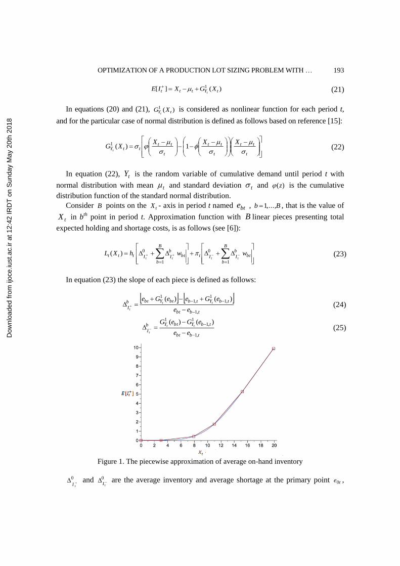
Figure 1. The piecewise approximation of average on-hand inventory

0

tI

and 0tI

are the average inventory and average shortage at the primary point te0 ,

Dow

nloa

ded

from

ijoc

e.iu

st.a

c.ir

at 1

2:42

IRD

T o

n S

unda

y M

ay 2

0th

2018



194

respectively. btw is the decision variable defined as the cumulative order amount through

the bth interval such that tbbtbt eew ,1 . Fig. 1 represent the linear approximation of ][ tIE in

which 10t and 10t . In this figure ][ tIE has been approximated via 5 linear pieces

(B=5). Since the expected functions are convex, the slopes b

I t and b

I t are increasing on b,

Bb ...,,1 . Therefore, due to the minimizing the objective function of the model, btw become

positive only when the previous variable, tbw ,1 reaches its maximum value, i.e.

tbtbtb eew ,2,1,1 . Therefore, we can set bt

B

b

t wX

1

in the mathematical model without

adding any axillary constraints. So piecewise linear approximation mathematical model of

SSDLSP is as follows:

T

t

K

k

tktkbt

B

b

b

IItbt

B

b

b

IIt

K

k

tkt clwwhuAcEMintttt

1 11

0

1

0

1

])()([}{ (26)

s.t.

B

b

B

b

tbbt

K

k

tk wwl

1 1

1,

1

Tt ,...,1 (27)

1

1

K

k

tku

Tt ,...,1 (28)

tktktk luq

Tt ,...,1 Kk ,...,1 (29)

tktktk uql )1( 1 Tt ,...,1 Kk ,...,1 (30)

tbbtbt eew ,1

Tt ,...,1 Bb ,...,1 (31)

}1,0{tku Tt ,...,1 Kk ,...,1 (32)

0btw

Tt ,...,1 Bb ,...,1 (33)

0tkl

Tt ,...,1 Kk ,...,1 (34)

3. SOLUTION APPROACH

If Sox’s model [10] is considered as a base model with specific solution, the proposed model

SSDLSP is more complex than the basic model in two ways. They are determining the

optimal discount levels in each period (determining the optimal amount of variables tku ) and

determining the optimal order quantity considering upper and lower limits of permitted

ordering. Our strategy to solve the problem is based on decomposition techniques. In this

paper, the problem SSDLSP is solved by branch and bound method. In each node of this

algorithm a sub-problem called P1, is solved by dynamic programming approach. At each

stage of this algorithm a sub-problem called P2 is raised which is solved by a branch and

bound method. In each node of the second branch and bound algorithm, sub-problem P3 is

solved by Lagrange relaxation method. In the remainder of this section, the solution

Dow

nloa

ded

from

ijoc

e.iu

st.a

c.ir

at 1

2:42

IRD

T o

n S

unda

y M

ay 2

0th

2018



195

approach is presented at four levels. In the first level, sub-problem P1 is presented and

branch and bound algorithm is described. In the second level, sub-problem P2 is defined and

solution of the sub-problem P1 is presented. In the third level, the solution to sub-problem P2

with the definition of P3 is discussed and at the last level, the solution to sub-problem P3 is

described.

3.1. First level

In this section, we first define the sub-problem P1 and then the solution of the problem with

branch and bound method is provided.

3.1.1 Definition of sub-problem P1

In this sub-problems, it is assumed that the discounting is permitted only for a set of periods,

call D, and for other periods, call R, purchase price is fixed to cheapest case (highest

discounts level) with no limit in ordering. Thus, the periods are considered in two sets R and

D. The collection of these two sets includes the complete planning horizon. In other words,

the constraints (4) to (8) are applied only for the periods of D. In each node of the branch

and bound algorithm the discount level for each period of D is specified, i.e. the variable tku

in period t, Dt , is 1 only for a specific discount level, say tm , and for other discount

levels, tmk , it is zero. Consequently, constraints (6) and (7) change into

1,1 tmttt

ttm qXXq .

For simplicity in model P1, the allowed upper and lower limits for ordering in period t are

shown by tu and tl , respectively. The unit purchase cost tc is defined as follows:

(35)

Rtc

Dtcc

tK

tmt

t

The mathematical model of the sub-problem P1 is as follows:

1

1

P1cEMin

ttt

T

t

tttt XXcXLsA (36)

s.t t1-tt uXX Dt (37)

t1-tt lXX

Dt (38)

t1-t XX

Tt ,...,1 (39)

t1-tt sXX M

Tt ,...,1 (40)

1,0ts Tt ,...,1 (41)

0tX

Tt ,...,1 (42)

In this model, the objective function is defined as in [10] and can be rewritten as follows:

Dow

nloa

ded

from

ijoc

e.iu

st.a

c.ir

at 1

2:42

IRD

T o

n S

unda

y M

ay 2

0th

2018



196

(43) ttt

T

t

tttt XccXLsA 1

1

P1cEMin

Property 1: If we set D as an empty set, the optimal solution of the problem P1 is a lower

bound for the problem SSDLSP.

Emptiness of set D means that the problem has no limits for ordering with regard to the

discount policies. Thus, by reducing the number of constraints, the solution space will get

greater. On the other hand, the best purchase price is considered for all periods. So the

obtained solution will be the best possible solution for the expected total cost.

Property 2: The optimal solution of sub-problem P1 is an upper bound for the problem

SSDLSP. The discounted cost structure and related constraints are incorporated only for the periods

of D and the purchase cost of other periods is set to the lowest case. Hence, it is obvious that

in this circumstance the obtained solution is a lower bound for the more restricted general

case of SSDLSP.

The main benefit of applying a B&B algorithm for solving SSDLSP is that it enumerates

all possible circumstances of variable tku , Tt ,...,1 , Kk ,...,1 , and solving the related sub-

problem. Therefore, the optimal solution to the problem SSDLSP is obtained by this

approach. In a complete enumeration, there is K quantities for discount level in each period

t, Tt ,...,1 . Hence, there are TK possible quantities for tku variable. The presented B&B

approach enumerate these cases implicitly.

3.1.1 The first level branch and bound algorithm

In this section, the steps of the branch and bound algorithm which breaks down SSDLSP to

P1 are presented.

To obtain an initial solution for the problem and use it as an lower bound from the

beginning of the B&B algorithm at the initial level, it is assumed that there are no ordering

constraints and the unit purchase price in all periods is the lowest possible value (maximum

discount). The solution space with this assumption is much larger than the original problem

and its objective function value is a lower bound for the problem. The problem with the

mentioned assumption is in fact, the problem introduced by Sox [10].

In Branching step of the algorithm, a period is selected and it is inserted to set D. The

strategy of selecting the period depends on the value of orders in the initial solution which is

in the root node. In other words, the periods with positive ordering value in the initial

solution are in priority of branching. More precisely, at the root node, a list of prioritizing

with the mentioned criterion is determined for branching and branching happens according

to this list for different periods. For each node, as a parent node, K nodes , as children node,

are generated by adding the related constraints for each discount level k , Kk ,...,1 . More

precisely, a period, say period t, is selected from the mentioned list and for each discount

level k , Kk ,...,1 , K nodes in period t is generating such that in each node a sub problem P1

with the upper and lower limit constraints , corresponding to the discount level k , is added

for the ordering value on period t. Branching continues from the active node that has the best

Dow

nloa

ded

from

ijoc

e.iu

st.a

c.ir

at 1

2:42

IRD

T o

n S

unda

y M

ay 2

0th

2018



197

lower bound. If two nodes with equal lower bound found, branching is done in the node that

has more depth in the search tree. After obtaining lower bound of each node by solving P1, the values of ordering are

calculated with their related prices I accordance with the discount cost structure to satisfy the

discount level constraints of that period. In this way, an upper bound is obtained for the

problem.

In this algorithm, nodes are fathomed with the following rules: 1. If the upper and lower bounds are equal in a node, it means that the resulting solution is

feasible and branching will not better the answer

2. If the lower bound of a node is greater than the best so far upper bound.

It should be noted that if the node is at the lowest level of the tree, the first rule is true about

it and the node is fathomed.

At the end of the algorithm, all nodes are fathomed and the node with the lowest

objective function whose is upper and lower limits are equal is the optimal solution.

3.2. Second level

To be an optimal algorithm, the B&B algorithm must solve the sub problem P1 in each node

optimally. For this purpose, a dynamic programming algorithm is applied that in each stage

a sub-problem, named P2, is raised.

3.2.1 Definition of sub problem P2 (s, t)

Consider a sub problem P1 raised in a node of B&B algorithm. Solving this sub problem by

our dynamic programming approach lead to be raised a sub problem ),(2 tsP in each stage

of the DP algorithm. In ),(2 tsP the goal is to find the minimum expected cost of holding,

ordering, purchasing and shortage from period s to the end of period t, assuming that the

ordering occurs only in the period s and if there are any discount constraints, in the period 1t

to mt with following conditions:

1. Period s and t+1 are two periods of sub problem P1 which do not have any ordering

constraint. (i.e. Rts 1, )

2. },...{ 1 mttM ( stm ) is the set of all the periods between s and t that have constraints in

ordering. ( DMttttts mm ,1,..., 110 )

Mathematical model of sub problem ),(2 tsP is as follows:

)(

0

1,

11 iiiii t

m

i

ttt

m

i

tsst XgsAAPMin

(44)

s.t iiii tttt suXX 1

mi ,...,1 (45)

iii ttt lXX 1 mi ,...,1 (46)

}1,0{it

s

mi ,...,1 (47)

0it

X

mi ,...,0 (48)

In equation (44), function )(, iji Xg expresses the expected total holding, shortage and

Dow

nloa

ded

from

ijoc

e.iu

st.a

c.ir

at 1

2:42

IRD

T o

n S

unda

y M

ay 2

0th

2018



198

purchase costs from period i to the end of period j when cumulative order from period i to

the end of period j is equal to the fixed amount iX . So )(, iji Xg is as follows.

(49)

j

it

tj

j

it

itiji

iji

iXLXc

jiXLXcc

Xg

0)(

0)()(

)(

001

1

,

In addition, total ordering cost is equal to the sum of ordering cost in period s and if any,

the ordering costs in 1t and mt . Equation (45) is a combination of the two constraints (37),

(40) and states that in the middle periods, if there is an order, its amount should not exceed

the upper limit of related discount level value of that period. It is notable that for the periods

that lower limit of discount level for them (it

l ) is greater than zero, the related variable it

s

will be one. Thus, that part of ordering cost which is variable is only considered for a subset

of MDz whose lower permissible limit of the discount level for them is zero since for

periods whose ordering amount are located on the first discount level we have 0it

l . Base

on what is stated above, we can rewrite the objective function of the model as equation (50).

(50) )(

0

1,

,1 iii

zi

ii

izi

i t

m

i

tt

Dt

tt

MtDt

tsst XgsAAAPMin

3.2.2 Dynamic programming algorithm

In this section, a forward dynamic programming is presented which solves the sub problem

P1 and in each its stage a sub problem ),(2 tsP must be solved. As mentioned earlier, a sub-

problem ),(2 tsP determines the optimal ordering policy from period s to the end of period t

named by optstX . In fact, opt

stX is a vector of optimal orders amount from period s to period t,

i.e. ),,...,( **1

*tss

optst XXXX , which minimizes the expected total cost during mentioned periods

under the mentioned assumption for sub problem ),(2 tsP . Let the minimum expected cost,

mentioned above, is denoted by )( optst

optst XP and suppose wt , Ww ,,...1 , be the periods of set R

where we have 1wt

s . In this case, the objective function of the sub problem can be

rewritten as the sum of several objective functions of the sub-problem ),(2 tsP :

(51)

W

w

optttttpwwww

XPcE

1

1,1, )(}{111

In equation (51) )(1,1,

11

opt

ttttwwww

XP

shows the optimal value of objective function of sub-

problem P2 from period wt to period 11 wt , when the optimal order quantity is equal to

Dow

nloa

ded

from

ijoc

e.iu

st.a

c.ir

at 1

2:42

IRD

T o

n S

unda

y M

ay 2

0th

2018



199

opt

tt wwX

1, 1. In this equation 11 Ttw . This equation indicates that sub problem P1 is separable

to sub problems )1,( 12 ww ttP .

The proposed dynamic programming algorithm has the following elements:

Stage: calculation of the minimum cost to period t ( Rt ).

State: Period s ( Rs ) as the last ordering period before the period t.

Recursive relationship: stf is the minimum cost associated with the ordering policy

form period s to t when the last order is occurred among the periods of R in period s and next

order in this set occurs at period 1t , we have

(52) )}()1(:{min)( 1,1,,

sXsXfXPf optst

optsksk

Rksk

optststst

If }|{ 1,1,optst

optsk

optsk XXX

then stf . This situation means that in the optimal policy

there is no policy by which it is possible to reach s, and then go to 1t , because this path

violates Constraint (39).

The pseudo code for the proposed algorithm is as follows

For t = 0,…,T and Rt 1 For s = 0,…t and Rs Solve ),(2 tsP and compute

opt

stX and )( opt

stst XP

If s = 0 , 0MIN Else

If )}()1(:,|{ 1, sXsXRkskk optst

optsk , MIN

Else

)}()1(:{min 1,1,,

sXsXfMIN optst

optsksk

Rksk

MINXPf opt

ststst )(

Tt

While 1t

if }{min,

ktRktk

jt ff

js

for j = s,…t, )( jXX optstj

)1( st

3.3 Third level

If the optimal values of binary ordering variables are determined in sub problem ),(2 tsP ,

then the problem will become a non-linear non-integer programming that convex

optimization methods can be used for optimal solving of the model.

3.3.1 Definition of sub problem P3

As previously mentioned, the collection zD is a series of periods between s and t where the

lower limit of order is zero. So in these periods ordering may be issued or not. A sub-

Dow

nloa

ded

from

ijoc

e.iu

st.a

c.ir

at 1

2:42

IRD

T o

n S

unda

y M

ay 2

0th

2018



200

problem P3 is the same as sub-problem P2 where it is decided beforehand for ordering in the

periods relating to set zD . In this case; periods of zD are divided into three categories. The

first set is AD where the cost of ordering for its member periods is determined accordance

with the terms defined in the sub-problem P2 and considered in the objective function of the

problem (whether there is an order in those periods or not), in other words 1it

s . The

second set is BD where the cost of ordering for its periods is considered as zero, and the

order is considered free in those periods. In other words )(0 Bit Dtsi

. The third set is CD

that is assumed not to perform any orders in those periods, in other words )(0 ciitDts .

Community of these three sets composes zD set.

Then for ease in model 3P the cost tA is defined as follows:

(53)

B

Att

Dt

DtAA

0

With this division for periods of zD the sub problem P2 changes into a problem where

there are no zero-one variables of ordering. Moreover, ordering occurs only in the period s

and in the periods of the series },...{ 1 nttN . This collection is a subset of M where ordering

variable for all its periods in the model P2 is equal to one ( 1it

s ). In other words, the period

of CD set has been removed from the collection of 1t to mt ( CDMN ).

Mathematical programming model of the problem 3P is as follows:

)(1,0

1 iii ttt

n

itst XgAPRMin

(54)

s.t iii ttt uXX 1 ni ,...,1 (55)

iii ttt lXX 1 ni ,...,1 (56)

0it

X

ni ,...,1 (57)

In this model, periods are assumed as follows: ),...,,1,...,( 1110 Nttttttts nnn

Property 3: In P3, if all periods of zD are placed in set BD , the optimal solution for sub

problem P3 would be a lower bound for sub problem ),(2 tsP .

Property 4: From any optimal solution of the sub problem P3, it is possible to reach an

upper bound for the sub problem 2P by modifying the order costs with regard to the solution

obtained.

Property 5: By complete enumeration of different values of variableit

s ( zi Dt ) and

solving the related sub problems, the optimal solution of P2 will be determined.

3.3.2 The third level branch and bound algorithm

In this section, in an algorithm similar to the mentioned branch and bound algorithm, a tree

Dow

nloa

ded

from

ijoc

e.iu

st.a

c.ir

at 1

2:42

IRD

T o

n S

unda

y M

ay 2

0th

2018



201

search based on the branch and bound approach is presented by which the it

s 's are

determined are determined in sub problem 2P and optimal value of ordering are obtained.

The initial solution for the root node of the branch and bound algorithm is considered as

follows. In 2P , variableit

s has appeared as a complicating variable. If we assume that in

each period, one can freely order and there is no charge for ordering, then the lower bound

of the problem is specified. Therefore, at the root node, ordering cost will be considered for

none of the periods of ZD and all the periods of ZD are placed in BD .

At the branching step of the algorithm, parent node is branched for a period from among

the periods of ZD . This branching generates two child nodes for a parent node where in one

the ordering cost is incurred and ordering is occurred in the mentioned period (the

mentioned period is placed in AD ) and the other one, the ordering cost is set to zero and no

ordering is occurred in the mentioned period. (the mentioned period is placed in CD ).

The strategy of node selection for branching is as follows. In this algorithm, among the

active nodes, the node with the best lower bound is selected for branching. If two nodes have

equal lower bounds, branching is done on the node with larger depth in the search tree.

In this algorithm, nodes are fathomed with the following fathoming rules:

If the upper and lower bounds are equal in a node, it means that the resulting solution is

feasible and branching would not lead to better solution.

If the lower bound of a node is greater than the upper bound obtained so far.

If for all periods of ZD the decision of ordering is determined. It means the node is

inactive and no further branching is needed.

The optimal solution of the sub problem will be obtained at the end of the algorithm.

Among the fathomed nodes, the node with the lowest objective function whose upper and

lower limits are equal is the optimal solution.

3.4 Fourth level The Lagrange relaxation method is used in cases whereby relaxing a number of constraints

of the problem leads to a more simple problem. In sub problem 3P , if the permissible lower

and upper limits of the order in equation (55) and (56) are relaxed, then the solution of the

relaxed problem can easily be obtained by derivative of the objective function. In this

section, the Lagrange relaxation method (LR) is presented to solving the sub problem 3P in

three main steps.

3.4.1 Step 1: Solving the relaxed version of 3P (RPP)

The Lagrange relaxed version of the sub problem 3P can be stated as follows:

(58)

n

i

tttlttttutttt

n

i

tst iiiiiiiiiiiilXXuXXXgARPPMin

1

1,

0111

s.t.

(59) 0it

X

ni ,,1

Dow

nloa

ded

from

ijoc

e.iu

st.a

c.ir

at 1

2:42

IRD

T o

n S

unda

y M

ay 2

0th

2018



202

Lagrange multipliers associated with the upper and lower limits of the ordering

constraints are iut and

ilt , respectively. We assume that 01100

nn utltltut .

Therefore, for each period like it , there are three variable it

X , ilt and iut . The objective

function of RPP can be rewritten as follows.

(60) iiiiiii

uttltttt

n

i

tst ulXfARPPMin 0

s.t.

(61) 0it

X

ni ,,1

where itit

Xf is defined as follows.

(62)

11

111.

i

i

iiiiiiiiii

t

tj

tjtltuttltutttt XLXccXf

Thus, the relaxed version of the sub problem 3P is an unconstrained non-linear

mathematical programming where its objective function is concave. Hence, its optimal

solution can easily be obtained by derivative. The partial derivative of the objective function

relative to it

X variable is as follows.

(63)

111

1 1

))(1)((

iiiiii

i

i

ij

i

iltuttltutt

t

tj

tyjjjt

tstccXFhh

X

XRPP

To find the roots of this function a combination of bisection method and false position

iteration methods are used.

3.4.2 Step 2: Updating the Lagrange multipliers

The main step in Lagrange relaxation is updating Lagrange multipliers for which in the

related literature, various methods have been developed. In these methods, the goal is to

maximize the dual problem of the original relaxed model via changing some coefficients of

Lagrange multiplier which subsequently leads to minimize original problem the original

variables. One of the main and general methods of updating Lagrange multipliers is using

sub-gradient method. For the sub-problem of 3P , Lagrange multipliers are updated as

follows:

(64) )()()()1(,0max

ututut Gt

(65) )()()()1(,0max

ltltlt Gt

Dow

nloa

ded

from

ijoc

e.iu

st.a

c.ir

at 1

2:42

IRD

T o

n S

unda

y M

ay 2

0th

2018



203

(66)

n

iutlt

best

GG

RPPUBt

1

2)(2)(

)(1

)()(

In these equations )(1

)()( ttut XXG and )(

1)()(

tttlt XXlG . Usually, in the

literature we found that 2)0( and for better convergence )( is reduced during iterations

of the algorithm. bestUB is the best upper bound obtained from the primary problem 3P that

are obtained in a heuristic way by making the solution feasible from the relaxed problem by

changing order amount to meet the feasible limits values of constraints. )(stRPP is the value

of the objective function of the relaxed problem in vth step.

3.4.3 Step 3: Stopping criteria

At this step, the predetermined convergence criteria are check to ensure that the obtained

solution is sufficiently close to the optimal solution to stop algorithm. Following criteria are

the main conditions stated in the literature.

If the difference of the best lower bound ( bestRPP ) with the best upper bound ( bestUB ) in

the algorithm is less than an error , the algorithm is terminated and the solution is reported

as -optimal solution.

If the number of occurrences is greater than a specified limit, the algorithm will stop.

If the vector of Lagrange multipliers are sufficiently close in the last iterations

( )()1()1( ), the algorithm will stop.

Overall Lagrange algorithm descried in this section is summarized in form of following

pseudo code.

Step 0: Initialization.

Set 1 ,

Initialize dual variables )(

Set

)1(

down

Step 1: Solution of the relaxed primal problem.

Solve the relaxed primal problem and obtain optimal value of )(x and its associated

objective function )(

Update the lower bound for the objective function of the primal problem,

If )()1(

down set )()( down

Step 2: Multiplier updating.

Update multipliers using sub-gradient method. If possible, update also the objective

function upper bound.

Step 3: Convergence checking.

If the stopping criterion is met, the -optimal solution is *)( xx and stop. Otherwise set

1 and go to Step 1.

Dow

nloa

ded

from

ijoc

e.iu

st.a

c.ir

at 1

2:42

IRD

T o

n S

unda

y M

ay 2

0th

2018



204

4. COMPUTATIONAL EXPERIENCE

Numerical experiments were carried out with the programming the proposed algorithm in C

# in Microsoft Visual Studio 2010. The results of solving the test problems are analyzed for

evaluating the performance of the algorithm. Also the results are compared with the results

obtained with the results obtained from solving the mixed-integer nonlinear model of

SSDLSP and mixed-integer linear approximation model which have been run in in

commercial optimization software GAMS. This comparison is performed based on

computational time and accuracy of solution by solving a set of random problems. Among

solver in GAMS only solvers BONMIN, KNITRO, ALPHAECP and LINDOGLOBAL are

available for MINLP models in which the first-order normal loss function is definable. The

only one of them which is able to announce the optimal solution on a small scale is

LINDOGLOBAL. Other solvers, even if they have reached the global optimum solution,

report it as a local optimal solution. So the basis of comparison of solution methods is to

solve the problem in GAMS with the solver LINDOGLOBAL. This solver can also be used

in LINGO software.

4.1 Experimental design

In generating test problems, each of the input data is a controlling factor. Among these

factors, the impact of two factors T and K are of more importance than other factors in

solving the problem. Other inputs have been adjusted experimentally and they have fixed

through all test problems. Ordering, holding, and shortage costs and initial inventory have

been set in accordance with reference [10]. The expected value of demand, )( tdE , for each

period is determined randomly. The standard deviation of demand for each period is

assumed as )(*2.0)( tt dEd like what has been done by [10]. Therefore, the expected value

and standard deviation of cumulative demand till period t, is equal to

t

j

jt dE

1

)( and

t

j

jt d

1

2 )( , respectively. The first level unit price of the unit purchasing price in

discounted cost structure in each period ( 1tc ) is determined randomly as shown in Table 1.

Also, Table 1 shows the adjusted values of other input parameters which have been

randomly generated.

Table 1: Adjusted values of the input parameters

tA th t 0I )( tdE 1tc Parameters

48 0.5 12 98 [20,120] [0,8] adjusted value

In setting the discount policy parameters, two factors are have great importance

generating test problems. The first one is k , the proportion of discount level to the average

demand by which the minimum ordering amount in kth level in the tth period, tkq , is

Dow

nloa

ded

from

ijoc

e.iu

st.a

c.ir

at 1

2:42

IRD

T o

n S

unda

y M

ay 2

0th

2018



205

determined i.e. tktkq . . The second important parameter is γ, the interest rate of discount,

which is an indicator to measure the purchase cost saving based on which the purchase cost

is obtained with the equation 1).1( tktk cc .

These two factors, similar to the Mirmohammadi et al. [4], have been set in deterministic

the lot sizing problem with quantity discount. Their value have been listed in Table 2 for

five discount levels.

Table 2: Adjusted value of parameters for discounting policy

5 4 3 2 K

5 4 3 2 k

0.125 0.1 0.075 0.05 k

To consider the cases for more than two random parameters t and 1tc , random generation

of data for each problem with T & K is repeated five times and the time to solve problems is

obtained from the average of five problems.

4.2. Analysis of test results

The average time to solve the problems are recorded from the implementation of the

program on the machine with specs Intel (R) core (TM) i7-2600 [email protected] GHz and they

have listed in Table 3. In this table, the mean of LG is the solver LINDOGLOBAL and B&B

refers to the proposed Branch and bound algorithm. Rt shows the average computational

time for every five test problems solved with various values of T and K in seconds. As

shown in Table 3, LG solver is unable to solve problems with more than 9 periods in the

specified time limit. N shows the number of instances of problems (from five instances)

which are solved optimally in a time less than 7200 seconds.

Table 3: Run time comparison of B&B and LG

LG B&B Num

4 3 2 4 3 2 K

N Rt N Rt N Rt Rt Rt Rt T

5 4.978 5 3.793 5 3.178 0.319 0.298 0.118 3 1

5 13.813 5 9.783 5 7.972 0.599 0.375 0.290 4 2

5 43.965 5 36.115 5 33.860 0.698 0.698 0.417 5 3

4 260 5 203 5 203 1.895 0.694 0.520 6 4

3 4049 5 1368 5 956 3.712 1.358 0.608 7 5

0 7200 1 7081 3 6194 3.710 2.846 0.939 9 6

0 7200 0 7200 0 7200 7.969 2.556 1.412 10 7

0 7200 0 7200 0 7200 8.996 5.201 2.432 11 8

Fig. 2 shows the computational time of B&B in comparison with solver LG with two

discount levels. As it is shown in this figure, the computational time of the B&B algorithm

is drastically less than the what is obtained from solver LG. This solver is not able to

Dow

nloa

ded

from

ijoc

e.iu

st.a

c.ir

at 1

2:42

IRD

T o

n S

unda

y M

ay 2

0th

2018



206

announce the optimal solution in 9 and 10 periods in a time less than 7200 sec.. This is while

the longest computational time of the proposed algorithm is for the case in which K=2 and

T=2 with time 2.432 seconds. This indicates the high performance of proposed algorithms.

Figure 2. Run time comparison of the solver B&B and LG with two discount level

Since in Fig. 2 changing the values relatively is not tangible, the bottom part of this graph

is magnified in Fig. 3.

Figure 3. Partial magnified of Figure 1

Two levels discount problem has more practical aspect than other variant of this problem.

Then the behavior of the proposed algorithm for two levels of discounts up to 30 periods is

compared. One of the main issues in the analysis of the behavior of nonlinear algorithms is

comparing them with their linear approximation version. In this respect, the approximation

model of the problem was encoded in GAMS software by considering 1000 approximation

points in each shortage function in the objective function. The computational results are

shown in Table 4. In this table, Rt is the average run time for all five instances. APP stands

for linear approximation model that runs on GAMS software. E means the relative error of

solution of approximation model to B & B algorithm. Num shows the problem number.

-801

199

1199

2199

3199

4199

5199

6199

7199

3 4 5 6 7 8 9 10

Rt

T

B&B

LG

0

1

2

3

4

5

6

7

8

3 4 5 6 7 8 9 10

Rt

T

B&B

LGDow

nloa

ded

from

ijoc

e.iu

st.a

c.ir

at 1

2:42

IRD

T o

n S

unda

y M

ay 2

0th

2018



207

Table 4: Run time comparison of B&B and APP

Num T B&B Rt APP Rt E

1 4 0.26 0.495 1.1

2 6 0.556 1.016 1.43

3 8 0.736 1.513 0.82

4 10 1.385 2.147 0.88

5 12 2.232 2.918 0.99

6 14 3.833 3.768 0.83

7 16 7.882 4.794 1.36

8 18 17.801 5.936 1.29

9 20 25.24 7.175 1.17

10 22 30.629 10.1 1.2

11 24 31.279 10.905 1

12 26 69.001 13.521 1.44

13 28 71.811 14.43 1.34

14 30 281.79 15.42 1.4

As shown in Fig. 4, the B&B algorithm gets the optimal solution faster than the

approximate model (APP). From this point of intersection of the curves in Fig. 4, the priority

of user should be specified, if the accuracy of the solution has higher priority, the proposed

B&B algorithm should be applied, and if the solution time is important, ignoring the relative

error, the approximation model is better.

Figure 4. Run time comparison of B&B and APP

5. RESULTS AND CONCLUSIONS

Adding the assumption of possibility of discount in material purchasing to the Sox’s model

[10] and deffining the stochastic single item lot sizing problem under quantity discount in

purchasing (SSDLSP) make the problem much more complex from two points of view.

Adding several binary variables to the model is the first aspect and the second one is the

extra constraints added to the base model. Thus, although the base model has been solved

01020304050607080

4 6 8 10 12 14 16 18 20 22 24 26 28

Rt

T

B&B

APP

Dow

nloa

ded

from

ijoc

e.iu

st.a

c.ir

at 1

2:42

IRD

T o

n S

unda

y M

ay 2

0th

2018



208

with a dynamic programming algorithm, the developed model of the algorithm has a more

complex solution approach. The proposed solution approach is presented at four levels based

on a branch and bound algorithm hybridized with a dynamic programming algorithm to

obtain the optimal solution of the problem. This approach can be used for any arbitrary

distribution of demand, and is faster than LINDOGLOBAL solver in GAMS. Furthermore,

to have a more precise evaluation of the presented algorithm in large scale problems, we

presented the linear approximate model of the model and we compared the presented

algorithm with it. The presented algorithm solves the problem with 30 periods (T=30)

optimally in a reasonable time, but, slower than approximate model. The approximate model

performs more efficient than B&B algorithm but with a bit of error to the optimal solution.

In our experiments, the maximum error of the approximate model is 1.44 percent which

seems tolerable regarding the speed of this approach.

In this paper we contained the shortage of product by charging the shortage cost to the

objective function of the problem. Since evaluating the shortage cost parameters may be

hard in practice, handling the shortage of products via defining the proper customer service

level may me more practical and it is left as a future development of the current work.

REFERENCES

1. Karimi B, Fatemi Ghomi S, Wilson J. The capacitated lot sizing problem: a review of

models and algorithms, Omega 2003; 31: 365-78.

2. Callerman T, Whybark D. Purchase quantity discounts in an MRP environment, Proceeding

of 8th A nnual Midwest Conference, 1977.

3. Chung, CS, Chiang DT, Lu CY. An optimal algorithm for the quantity discount problem, J

Oper Manag 1987; 7: 165-77.

4. Mirmohammadi SH, Shadrokh S, Kianfar F. An efficient optimal algorithm for the quantity

discount problem in material requirement planning, Comput Oper Res 2009; 36: 1780-88.

5. Goossens DR, Maas A, Spieksma FC, Van de Klundert J. Exact algorithms for procurement

problems under a total quantity discount structure, European J Oper Res 2007; 178: 603-26.

6. Tempelmeier H. Stochastic lot sizing problems, Handbook of Stochastic Models and

Analysis of Manufacturing System Operations 2013, Springer, pp. 313-44.

7. Silver E. Inventory control under a probabilistic time-varying, demand pattern, AIIE Trans

1978, 10: 71-9.

8. Bookbinder JH, Tan JY. Strategies for the probabilistic lot-sizing problem with service-level

constraints, Manag Sci 1988; 34: 1096-1108.

9. Vargas V. An optimal solution for the stochastic version of the Wagner–Whitin dynamic lot-

size model, European J Oper Res 2009; 198: 447-51.

10. Sox CR. Dynamic lot sizing with random demand and non-stationary costs, Oper Res

Letters 1997; 20: 155-64.

11. Tempelmeier H. On the stochastic uncapacitated dynamic single-item lotsizing problem with

service level constraints, European J Oper Res 2007; 181: 184-94.

12. Vargas V, Metters R. A master production scheduling procedure for stochastic demand and

rolling planning horizons, Int J Product Economics 2011; 132: 296-302.

Dow

nloa

ded

from

ijoc

e.iu

st.a

c.ir

at 1

2:42

IRD

T o

n S

unda

y M

ay 2

0th

2018



209

13. Haji M, Haji R, Darabi H. Price discount and stochastic initial inventory in the newsboy

problem, J Indust Syst Eng 2007; 1: 130-8.

14. Kang HY, Lee AH. A stochastic lot-sizing model with multi-supplier and quantity discounts,

Int J Product Res 2013; 51: 245-63.

15. Rossi R, Kilic OA, Tarim SA. Piecewise linear approximations for the static–dynamic

uncertainty strategy in stochastic lot-sizing, Omega 2015; 50: 126-40.

Dow

nloa

ded

from

ijoc

e.iu

st.a

c.ir

at 1

2:42

IRD

T o

n S

unda

y M

ay 2

0th

2018


Documents

OPTIMIZATION OF A PRODUCTION LOT SIZING …ijoce.iust.ac.ir/article-1-245-en.pdfOPTIMIZATION OF A PR ODUCTION LOT SIZING PROBLEM WITH QUANTITY DISCOU NT S. Khosravi and S.H. Mirmohammadi*,