Economic Lot Sizing and Scheduling in Distributed

Journal of Optimization in Industrial Engineering Vol.12, Issue 1, Winter and Spring 2019, 103- 117

DOI: 10.22094/JOIE.2018.542997.1510

103

Economic Lot Sizing and Scheduling in Distributed Permutation Flow Shops

Mohammad Alaghebandha a, Bahman Naderi a,*, Mohammad Mohammadi

aDepartment of Industrial Engineering, Faculty of Engineering, Kharazmi University, Tehran, Iran

Received 25 August 2017; Revised 29 June 2018; Accepted 02 July 2018

Abstract This paper addresses a new mixed integer nonlinear and linear mathematical programming economic lot sizing and scheduling problem in distributed permutation flow shop problem with number of identical factories and machines. Different products must be distributed between the factories and then assignment of products to factories and sequencing of the products assigned to each factory has to be derived. The objective is to minimize the sum of setup costs, work-in-process inventory costs and finished products inventory costs per unit of time. Since the proposed model is NP-hard, an efficient Water Cycle Algorithm is proposed to solve the model. To justify proposed WCA, Monarch Butterfly Optimization (MBO), Genetic Algorithm (GA) and combination of GA and simplex are utilized. In order to determine the best value of algorithms parameters that result in a better solution, a fine-tuning procedure according to Response Surface Methodology is executed. Keywords: Lot sizing; Distributed permutation flow shops; Linearization; Water Cycle Algorithm; Monarch butterfly optimization.

1. Introduction Economic Lot Sizing Problems (or ELSP) is one of the well-recognized production planning problems belonging to the medium-term decision making. It attracts many attentions in the literature after the pioneer papers of Rogers (1958) and Elion (1959). In classic ELSP, there are a set of products need to be processed on a single machine. The machine can process at most one product at a time. Both demand and production of each product follow constant rates and are known in advance. All the demands must be satisfied; that is, no shortage is allowed. Some setup is carried out before the production can commence. This setup could be influential regarding both its magnitude of time and its cost. Moreover, the production horizon is assumed to be continuous and infinite. The objective is to specify a production schedule so as to minimize long-run average total cost, i.e. sum of setup and inventory holding costs. The cyclic schedule is frequently assumed to be common cycle; that is, the production cycle times of all the products are the same. The production schedule includes two decision dimensions, sequence and quantity in which products are processed (Maxwell, 1964). Karimi et al. (2003) provide a review of models and algorithms for different lot sizing problems. In practice, there are shops in which a series of operations have to be carried out to turn raw materials into finished products. One of the commonly-happening environments is to have the same route for all the products to pass through machines. In this case, the shop is called a flow shop. If it is assumed that sequences of products on all machines are the same, the shop is called a permutation flow shop. To

approach realistic industrial settings, the classic problem is further developed to consider Economic Lot Sizing Problems in Permutation Flow shops (or ELSP in PFS). It seems that multi-stage ELSP was initiated by El-Najdawi (1989) through considering a two-stage problem. Later, the problem is developed to the case of arbitrary number of stages by Hsu and El-Najdawi (1990). Looking into the literature of this problem, is noticed that it experiences a new era after the late 90s. Before 1999, researches are centered on this idea that production sequence is negligible due to its trifling influence on the total cost. Therefore, the little heed was paid to the sequence decision. It was common place to tackle the problem by minimizing the total cost for a given sequence usually obtained by a simple heuristic. As a case for this point, the reader refers to a paper by El-Najdawi and Kleindorfer (1993). They make use of Shortest Processing Time (or SPT) to obtain a sequence. Their core contribution is on lot-sizing decision rather than sequencing decision. Dobson and Yano (1994) and El-Najdawi (1992, 1994) are among the other papers considering ELSP in PFS. But, they still more concentrate on lot-sizing decision. Ouenniche et al. (1999) studied ELSP in PFS, and explored the effect of sequencing decision on the final total cost. They concluded that sequencing decision should be taken into account as well as lot-sizing one. They present a MINLP model and some heuristics in two groups: constructive heuristics (CH) and improvement heuristics, commonly known as metaheuristics. Contrary to existing CHs in the literature of PFS usually minimizing completion time related objectives, they propose CHs that minimize the work-in-process holding cost. Afterwards, they present some local search procedures improving the solutions obtained by CHs as a metaheuristic. *Corresponding author Email address: bahman.naderi@ aut.ac.ir*Corresponding author Email address: bahman.naderi@ aut.ac.ir

a

Mohammad Alaghebandha et al. /Economic Lot Sizing and Scheduling…

104

Later, Torabi et al. (2005) develop the problem considering presence of multiple identical machines at each stage; and they solve the problem by adaptation of the solution method previously presented by Ouenniche et al. (1999). Akrami et al (2006) addressed the common cycle multi-product lot sizing and scheduling problem in deterministic flexible flow shops where the planning horizon is finite and fixed by management and the production stages are in series, while separated by finite intermediate buffers. They used both genetic algorithm and tabu search methods to find an optimal or near-optimal solution for the problem. A differential evolution (DE) based memetic algorithm, named ODDE, is proposed by Li and Yin (2013) for permutation flow shop problem with minimizing makespan and maximum lateness objectives. Rahman et al (2015) considered a make -to stock production system, where three related issues must be considered: the length of a production cycle, the batch size of each product, and the order of the products in each cycle. To deal with these tasks, they proposed a Genetic Algorithm based lot scheduling approach with an objective of minimizing the sum of the setup and holding costs. Bargaoui et al (2017) addressed the Distributed Permutation Flow shop Scheduling Problem with an artificial chemical reaction metaheuristic which objective is to minimize the maximum completion time. In the proposed CRO, the effective NEH heuristic is adapted to generate the initial population of molecules. Viagas et al (2018) addressed the distributed permutation flow shop scheduling problem to minimize the total flow time. They first analyzed it and discussed several properties, theorems, assignment rules, representation of the solutions and speed-up procedures. They proposed an iterative improvement algorithm to further refine the so-obtained solutions. Rifai et al (2016) propose a novel model of the developed distributed scheduling by supplementing the reentrant characteristic into the model of distributed reentrant permutation flow shop scheduling. This Problem is described as a given set of jobs with a number of reentrant layers are processed in the factories, which comprises a set of machines, with the same properties. The aim of the study is to minimize makespan, total cost and average tardiness. Recently, Naderi and Ruiz (2009) have introduced a new generalization of the permutation flow shop originated from today companies’ structure in which factories are merged to build a common enterprise. The purpose is to obtain higher productive, less production cost and so on. More details could be found in Wang (1997). In these enterprises, production planners are to handle more complicated decision making processes. In single-factory problems, there are still two above-mentioned decisions, whereas in the distributed problem another decision appears: the assignment of the products to suitable factories. Consequently, three decisions have to be taken; product allocation to factories, product scheduling at each factory as well as lot sizing decision. Based on the best reviewed, this paper is the first study on the Economic Lot Sizing Problem in Distributed Permutation Flow Shop (or ELSP in DPFS). This problem is a well- known scheduling problem in many industries, such as steel, pharmaceutical, automobile, and food processing

(Naderi and Ruiz, 2010). The paper contributes by developing two different alternative Mixed Integer Non-Linear Programming (or MINLP) models according to previous paper Ouenniche et al. (1999) in Distributed manner. This allows for a precise characterization of the ELSP in DPFS. The models’ specifications are precisely compared. Apart from the MIP models, four metaheuristics based on Monarch Butterfly Optimization, Water Cycle Algorithm, Genetic Algorithm and Genetic Algorithm with Simplex are presented. The metaheuristic’s performance is evaluated by comparing against the optimal solutions obtained by the linear models in small, medium and large sized problems. The rest of the paper is organized as follows. Section 2 develops two mathematical models and linearization of the proposed models through discussion. Section 3 introduces four presented metaheuristics. Section 4 evaluates the performance of the models and the algorithms. Section 5 concludes the paper and clarifies some directions for future studies.

2. Mathematical Models Mathematical models are known to be the best way to precisely define all the characteristics of a problem. Actually, by mathematical models, it is possible to turn the implicit explanations of a novel problem into the explicit and detailed ones. Moreover, mathematical models could be a starting point for many solution methods such as problem-specific branch-and-bound methods, approximation algorithms or even metaheuristics. Apart from being a starting point in many different algorithms, recently they could also be treated as solution methods because of available specialized software and high capacity computers. Considering all these together encourage researchers to develop effective mathematical models for their corresponding problems. More formally, the problem of ELSP in DPFS could be described as follows: a set of different customer demands with different quantities are received. To fulfill them, raw materials of each demand could be operated in each of available different factories each of which has the same set of

machines deposed in series. There is no restriction on allocation of customer demands to the factories; however, all of a demand must be manufactured in one factory. When a demand is assigned to a factory, it could not be transferred to another factory. It is also considered that the production rate of each demand is not changed from factory to factory. Before the production of a product can begin on a machine, some anticipatory setup must be performed, meaning that, the setup of a product on a machine can start when the machine finishes the process of the previous product (even if product is processed on machine i-1). A product cannot be processed by more than one machine at a time; and a machine cannot process more than one product at a time. There is no maintenance or breakdown, i.e. machines are always available. Customer demands are only for finished products which continuously delivered. Demand and production rates, setup times and costs, and inventory holding costs are deterministic and constant over an infinite planning horizon. Each product has a unique production rates


105

on different machines. Inventory levels and holding time directly determine the inventory holding costs. Shortages are not allowed. When the operation of a product starts, it cannot be interrupted, i.e. products are not preemptive. There is unlimited buffer between machines, i.e. products can wait unlimitedly for the next machine. It is additionally assumed that the production cycle times of all the factories are equal. In this section, the problem by two different MIP models are formulated, since it is not clear which model has best performance. Notice that the objective function of the models includes three parts: setup cost, inventory holding cost of finished and semi-finished products. A continuous variable denoting the common cycle time is employed in two models. Before presenting the models, the parameters and indices, shown in Table 1, are defined. Table 1 The parameters and indices used in the models

Notation Description

Number of products

Number of machines

Number of factories

,

Index for products, , 1, 2, … ,

Index for machines, 1, 2, … ,

Index for factories, 1, 2, … ,

,

Production rate of product on machine

Demand rate of end product

,

Setup time of product on machine

Total setup cost of product over all machines

,

Inventory holding cost per unit of product per time unit between machines and +1

Inventory holding cost per unit of finished product per time

Big positive number

2.a. Model 1

In this model, Binary Variables (or BV) just represent the position of products in sequence. Contrary to the next model, the two decisions of product allocation to factories and product sequence in each factory are together determined by one BV type. Notice that notation is an index to denote positions and , is start time of product on machine that works in a similar , in model 2. The following variables are defined in this model:

, , : Binary variable that takes value 1 if product occupies position in factory , and 0 otherwise. (1)

, , : Continuous variable for the starting time of the product in position on machine in factory . (2)

Model 1 characterizes the ELSP in DPFS as follow: Minimize Z ∑

T∑ h 1

,

∑ h ,, ,

· T (3)

∑ ∑ ∑ ∑ X , , h , · d S , , S , ,

Subject to:

∑ ∑ X , , 1 (4)

∑ X , , 1 , (5)

SS , SS ,·T

, , (6)

SS , SS ,·T

,st ,

M 1 X , , M 1 X , , , , , ,

,

(7)

SS , st , , (8)

T SS ,·T

,st , SS ,

M 1 X , , M 1 X , , , , , ,

,

(9)

T ∑ ∑ X , , · st ,·T

, , (10)

SS , ∑ ∑ X , , . S , , , (11) T, S , , 0 , , (12) X , , 0, 1 , , (13) The objective function (3) is to minimize the sum of setup costs, work-in-process inventory costs and finished products inventory costs per unit of time. Constraint set (4) assures that every product must be assigned once. Constraint set (5) ensures that every position must be occupied once. Constraint set (6) states that the process of a product on machine cannot begin before its process on machine i-1 completes. Constraint sets (7) is the dichotomous pairs of constraints relating each possible production. Constraint set (8) ensures that the first product in each factory starts after its setup. Constraint set (9) and (10) ensure the minimum possible cycle time is satisfied. This minimum is obtained through capacity-constrained of each factory. Constraint set (11) ensures that each product in every position must be occupied in one factory. Constraint sets (12) and (13) define the decision variables.

2.b. Model 2

In this model there are two types of Binary Variables. The first one is to show relative sequence of every pair of products, meaning that, whether a product precedes/succeeds another product or not. The other BV is to represent product allocation to factories. The variables employed in this model are:

, : Binary variable that takes value 1 if product follows product , and 0 otherwise. (14)

, : Binary variable that takes value 1 if product is

processed in factory , and 0 otherwise. (15)

, : Continuous variable for the starting time of product

on machine . (16)

Model 2 formulates the ELSP in DPFS as follow:

Minimize Z ∑T

∑ h 1,

∑ h ,, ,

· T (17)

∑ ∑ h , · d S , S ,

Subject to:

∑ Y , 1

(18)


106

S , S ,·T

, , (19)

S , S ,·T

,st , M 1

X , M 1 Y , M 1 Y , , , , (20)

S , S ,·T

,st , M · X ,

M 1 Y , M 1 Y , , , , (21)

T S ,·T

,st , S ,

M 1 X , M 1 Y ,

M 1 Y ,

, , , (22)

T S ,·T

,st , S , M ·

X , M 1 Y , M 1 Y , , , , (23)

T ∑ Y , · st ,·T

, , (24)

S , st , , (25) X , X , 1 , , (26)

T, S , 0 , (27)

X , 0, 1 , (28)

Y , 0, 1 , (29)

The objective function (17) is to minimize the sum of setup costs, work-in-process inventory costs and finished products inventory costs per unit of time. Constraint set (18) ensures that every product is allocated exactly to one factory. Constraint set (19) states that the process of a product on machine cannot begin before its process on machine i-1 completes. Constraint sets (20) and (21) are the dichotomous pairs of constraints relating each possible production pair. In other words, they assure that a machine processes at most one product at a time. Constraint sets (22) and (23) calculate the common cycle time, whereas Constraint set (24) specifies the capacity-constraints of each factory to manufacture assigned products. Constraint set (25) ensures that the first product in each factory starts after its setup. Constraint set (26) avoids the occurrence of cross-precedence, meaning that a product cannot be at the same time both a predecessor and a successor of another product. Constraint sets (27), (28) and (29) define the decision variables.

2.1 Linearization of the proposed model

The proposed models are MINLP because of the nonlinear term in the objective function and also constraints. In order to decrease the number of nonlinear terms, linearization in a similar way as in Rodriguez et al (2014), You and Grossmann (2008) and Pakzad-Moghaddam et al. (2014) is used. In the model 1, the bilinear terms between the continuous variable T and the binary variables X , , in objective function, also constraints (10 and 11), are linearized as follows. Notice that constraint set (11) have been replaced with constraint sets (30) – (33), and constraint (34) of the first derivative of the objective function is obtained.

Minimize ∑∑

∑,

∑ , , ,

∑ . ∑1

,

∑ ,, ,

∑ ∑ ∑∑ , , , , , , .

, ·

Subject to:

Eq. (4) – Eq. (10) and Eq. (12) – Eq. (13)

, , , , , . , , , (30)

, , , , , 1 , , . , , , (31)

, , , , , 1 , , . , , , (32)

, , , 0 , , , (33) Minimize∑

∑

∑,

∑ , , ,

21

,, 2

1

,

1

,·

, · , ,

Subject to: Eq. (18) – Eq. (24) and Eq. (25) – Eq. (29)

∑

∑1

,

∑ ,, ,

(34)

In a similar way in the model 2, one term in objective function is divided by continuous variable (T) and constraint (24), the bilinear terms consisting of a continuous variable (T) product a binary variable Y , are must be linearized as follows.

3. Complexity and Test Problems

The performance of the models and method is studied through its solutions for a total of 180 problems in small, medium and large sized. Different problem sets with 3, 5 or 10 products and 3, 4, 5, 8, 10 or 15 machines and 2, 4, 5, 6 and 10 factories in three sized are considered. Each problem set is composed of 20 randomly generated problems as follows in Table 2 and 3. There are 9 combinations of n, m and g. Twenty instances for each combination for a total of 180 instances are generated.


107

Table 2 Generate of the test problems

Parameter Description

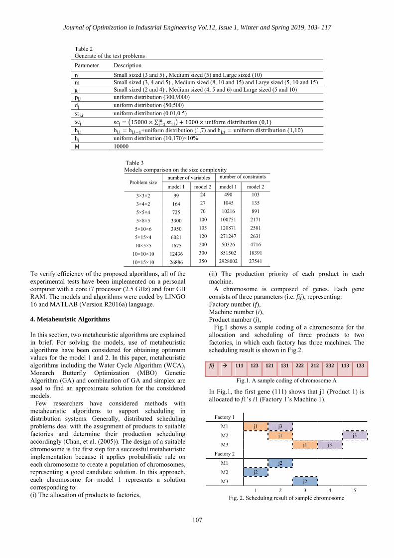
n Small sized (3 and 5) , Medium sized (5) and Large sized (10) m Small sized (3, 4 and 5) , Medium sized (8, 10 and 15) and Large sized (5, 10 and 15) g Small sized (2 and 4) , Medium sized (4, 5 and 6) and Large sized (5 and 10) p , uniform distribution (300,9000)

d uniform distribution (50,500)

st , uniform distribution (0.01,0.5)

sc sc 15000 ∑ st , 1000 uniform distribution 0,1 h , h , h , +uniform distribution (1,7) and h , uniform distribution 1,10 h uniform distribution (10,170)×10%

M 10000

Table 3 Models comparison on the size complexity

Problem size number of variables number of constraints

model 1 model 2 model 1 model 2

3×3×2 99 24 490 103

3×4×2 164 27 1045 135

5×5×4 725 70 10216 891

5×8×5 3300 100 100751 2171

5×10×6 3950 105 120871 2581

5×15×4 6021 120 271247 2631

10×5×5 1675 200 50326 4716

10×10×10 12436 300 851502 18391

10×15×10 26886 350 2928002 27541 To verify efficiency of the proposed algorithms, all of the experimental tests have been implemented on a personal computer with a core i7 processor (2.5 GHz) and four GB RAM. The models and algorithms were coded by LINGO 16 and MATLAB (Version R2016a) language.

4. Metaheuristic Algorithms

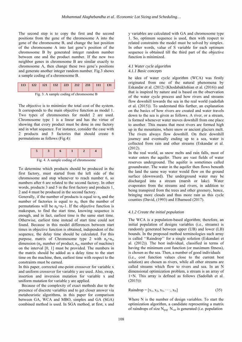
In this section, two metaheuristic algorithms are explained in brief. For solving the models, use of metaheuristic algorithms have been considered for obtaining optimum values for the model 1 and 2. In this paper, metaheuristic algorithms including the Water Cycle Algorithm (WCA), Monarch Butterfly Optimization (MBO) Genetic Algorithm (GA) and combination of GA and simplex are used to find an approximate solution for the considered models. Few researchers have considered methods with metaheuristic algorithms to support scheduling in distribution systems. Generally, distributed scheduling problems deal with the assignment of products to suitable factories and determine their production scheduling accordingly (Chan, et al. (2005)). The design of a suitable chromosome is the first step for a successful metaheuristic implementation because it applies probabilistic rule on each chromosome to create a population of chromosomes, representing a good candidate solution. In this approach, each chromosome for model 1 represents a solution corresponding to: (i) The allocation of products to factories,

(ii) The production priority of each product in each machine. A chromosome is composed of genes. Each gene consists of three parameters (i.e. fij), representing: Factory number (f), Machine number (i), Product number (j), Fig.1 shows a sample coding of a chromosome for the allocation and scheduling of three products to two factories, in which each factory has three machines. The scheduling result is shown in Fig.2. fij 111 123 121 131 222 212 232 113 133

Fig.1. A sample coding of chromosome A

In Fig.1, the first gene (111) shows that j1 (Product 1) is allocated to f1’s i1 (Factory 1’s Machine 1).

Factory 1

M1 j1 j3

M2 j1 j3

M3 j1 j3

Factory 2

M1 j2

M2 j2

M3 j2

1 2 3 4 5

Fig. 2. Scheduling result of sample chromosome


108

The second step is to copy the first and the second positions from the gene of the chromosome A into the gene of the chromosome B, and change the last position of the chromosome A into last gene’s position of the chromosome B by generated integer random number between one and the product number. If the new two neighbor genes in chromosome B are similar exactly to chromosome A, then change these two gene’s positions and generate another integer random number. Fig.3 shows a sample coding of a chromosome B.

113 122 121 132 223 212 233 111 131

Fig. 3. A sample coding of chromosome B

The objective is to minimize the total cost of the system. It corresponds to the main objective function as model 1. Two types of chromosomes for model 2 are used. Chromosome type 1 is a linear and has the virtue of showing that every product must be done in one factory and in what sequence. For instance, consider the case with 2 products and 5 factories that should create 6 permutations as follows (Fig.4):

5 3 6 1 2 4

Fig. 4. A sample coding of chromosome

To determine which products should be produced in the first factory, must started from the left side of the chromosome and stop whenever to reach number 6, so numbers after 6 are related to the second factory. In other words, products 3 and 5 in the first factory and products 1, 2 and 4 must be produced in the second factory. Generally, if the number of products is equal to np and the number of factories is equal to nf, then the number of permutations will be np+nf-1. If the objective function is makespan, to find the start time, knowing sequence is enough, and in fact, earliest time is the same start time. Otherwise, earliest time instead of start time could not found. Because in this model differences between start times in objective function is obtained, independent of the sequence, the delay time should be calculated. For this purpose, matrix of Chromosome type 2 with np×nm

dimension (np: number of product, nm: number of machine) on the interval [0, 1] must be provided. The numbers in the matrix should be added as a delay time to the start time on the machine, then, earliest time with respect to the constraints must be earned. In this paper, corrected one-point crossover for variable x and uniform crossover for variable y are used. Also, swap, insertion and inversion mutation for variable x and uniform mutation for variable y are applied. Because of the complexity of exact methods due to the presence of discrete variables and to get closer answer via metaheuristic algorithms, in this paper for comparison between GA, WCA and MBO, simplex and GA (SGA) combined method is used. In SGA method, at first, x and

y variables are calculated with GA and chromosome type 1. So, optimum sequence is used, then with respect to related constraints the model must be solved by simplex. In other words, value of S variable for each optimum sequence is obtained till the third part of the objective function is minimized.

4.1 Water cycle algorithm 4.1.1 Basic concepts

he idea of water cycle algorithm (WCA) was firstly originated from one of the natural phenomena by Eskandar et al. (2012) (Khodabakhshian et al. (2016)) and that is inspired by nature and is based on the observation of the water cycle process and how rivers and streams flow downhill towards the sea in the real world (sadollah et al. (2015)). To understand this further, an explanation on the basics of how rivers are created and water travels down to the sea is given as follows. A river, or a stream, is formed whenever water moves downhill from one place to another. This means that most rivers are formed high up in the mountains, where snow or ancient glaciers melt. The rivers always flow downhill. On their downhill journey and eventually ending up to a sea, water is collected from rain and other streams (Eskandar et al. (2012). In the real world, as snow melts and rain falls, most of water enters the aquifer. There are vast fields of water reserves underground. The aquifer is sometimes called groundwater. The water in the aquifer then flows beneath the land the same way water would flow on the ground surface (downward). The underground water may be discharged into a stream (marsh or lake). Water evaporates from the streams and rivers, in addition to being transpired from the trees and other greenery, hence, bringing more clouds and thus more rain as this cycle counties (David, (1993) and Elhameed (2017).

4.1.2 Create the initial population

The WCA is a population-based algorithm; therefore, an initial population of designs variables (i.e., streams) is randomly generated between upper (UB) and lower (LB) bounds. In the proposed method terminologies such array is called ‘‘Raindrop’’ for a single solution (Eskandari et al. (2012)). The best individual, classified in terms of having the minimum cost function (or maximum fitness), is chosen as the sea. Then, a number of good individuals (i.e., cost function values close to the current best solution) are chosen as rivers, while all other streams are called streams which flow to rivers and sea. In an N dimensional optimization problem, a stream is an array of 1×N. This array is defined as follows (Sadollah et al. (2015)):

Raindrop = [x1, x2, x3, · · ·, xN] (35)

Where N is the number of design variables. To start the optimization algorithm, a candidate representing a matrix of raindrops of size Npop Nvar is generated (i.e. population

ofrannure

TthDeabwathvaanfo(2

Cn

Wto reea(i.(3thstrberiv(fiofva

4.

Acafanmothsewhcygadirarr

Jou

f raindrops). Hndomly is giv

umber of popuspectively) (E

Then, a numbee rest of thepending on t

bsorb water fater in a streae other strea

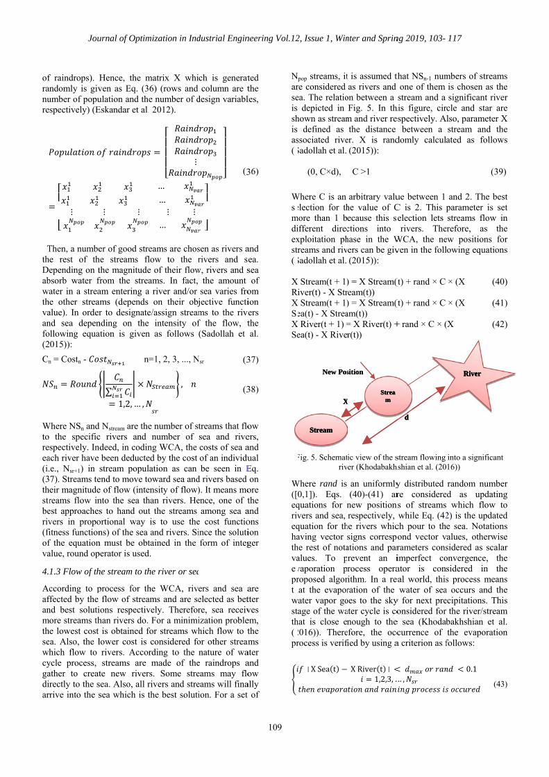
alue). In ordernd sea depenllowing equa015)):

n = Costn -

Where NSn andthe specific

spectively. Inach river have e., Nsr+1) in 7). Streams teeir magnitudereams flow inest approachesvers in propoitness functionf the equationalue, round op

1.3 Flow of th

ccording to pffected by the nd best solutiore streams the lowest cost a. Also, the lhich flow to

ycle process, ather to creatrectly to the srive into the s

urnal of Optim

Hence, the mven as Eq. (3ulation and theEskandar et al.

er of good strehe streams flthe magnitudefrom the streaam entering aams (depends r to designate

nding on the ation is given

n=

∑1,2, … ,

d Nstream are thec rivers and ndeed, in codin

been deductestream popul

end to move toe of flow (intento the sea ths to hand outortional way ns) of the sea n must be obtperator is used

he stream to th

process for thflow of strea

ions respectivhan rivers do. is obtained f

lower cost is rivers. Accorstreams are

te new riversea. Also, all rsea which is t

mization in Ind

matrix X whi (rows and

e number of d 2012).

…

… …

eams are choslow to the re of their flowams. In fact,

a river and/or on their obj

e/assign stream intensity of

n as follows

=1, 2, 3, ..., N

,

e number of snumber of

ng WCA, the ed by the cost lation as can oward sea andensity of flow)han rivers. Het the streams is to use theand rivers. Si

tained in the d.

he river or sea

he WCA, rivams and are sevely. Therefor

For a minimifor streams whconsidered fording to the made of the

rs. Some strerivers and strethe best soluti

dustrial Engin

ch is generatcolumn are t

design variabl

(3

sen as rivers arivers and se

w, rivers and sthe amount

sea varies frojective functims to the rivef the flow, t(Sadollah et

Nsr (3

(3

treams that flosea and rivecosts of sea aof an individube seen in E

d rivers based ). It means moence, one of t

among sea ae cost functioince the solutiform of integ

a

ers and sea aelected as betre, sea receivization problehich flow to tor other streamnature of wa

e raindrops aeams may floeams will finaion. For a set

neering Vol.12

109

ted the les,

36)

and ea. sea of

om ion ers the al.

37)

38)

ow ers, and ual Eq. on

ore the and ons ion ger

are tter ves em, the ms

ater and ow

ally of

Narseis shis as(S

X

Wsemdiexstr(S

XRXSeXSe

F

W([eqriveqhathvaevprthwstth(2pr

2, Issue 1, Win

Npop streams, itre considered ea. The relatio

depicted in hown as stream

defined as ssociated riveSadollah et al.

X� (0, C×d),

Where C is an election for th

more than 1 bifferent direcxploitation phreams and riv

Sadollah et al.

X Stream(t + 1)iver(t) - X Str

X Stream(t + 1)ea(t) - X Strea

X River(t + 1) =ea(t) - X Rive

Fig. 5. Schematriv

Where rand is 0,1]). Eqs. quations for nvers and sea, quation for thaving vector he rest of notaalues. To pvaporation proposed algorhat the evapor

water vapor goage of the wa

hat is close e2016)). Thererocess is verif

X Sea t

SSStttrrreeeaaammm

New PosNew Pos

XXX

nter and Sprin

t is assumed tas rivers and

on between a Fig. 5. In th

m and river rethe distance

er. X is rand(2015)):

C >1

arbitrary valuhe value of Cecause this sctions into hase in the Wvers can be giv

(2015)):

) = X Stream(ream(t)) ) = X Stream(am(t)) = X River(t) +r(t))

ic view of the ser (Khodabakh

an uniformly(40)-(41) ar

new positionrespectively,

he rivers whicsigns correspations and parrevent an irocess opera

rithm. In a reration of the oes to the skyater cycle is conough to the

efore, the occfied by using a

X River t1,2,3, …

SSStttrrreeeaaammm

sition sition

XX

ng 2019, 103-

that NSn-1 numone of them stream and a

his figure, cirespectively. A

between a domly calcula

ue between 1 C is 2. This pselection lets

rivers. TheWCA, the neven in the foll

(t) + rand × C

(t) + rand × C

+ rand × C × (

stream flowing hshian et al. (20

y distributed re considere

ns of streams while Eq. (42

ch pour to thpond vector vrameters consimperfect coator is conseal world, this

water of seay for next preonsidered for

e sea (Khodabcurrence of a criterion as f

… ,

ddd

117

mbers of streais chosen as significant rivcle and star lso, parameterstream and ated as follo

(3

and 2. The bparameter is streams flowrefore, as

ew positionsowing equatio

× (X (4

× (X (4

(X (4

into a significa16))

random numbd as updatiwhich flow

2) is the updae sea. Notatioalues, otherwsidered as scaonvergence, sidered in s process mea

a occurs and ecipitations. T

the river/strebakhshian et the evaporati

follows:

0.1

(

RRRiiivvveeerrr

ams the ver are r X the

ows

39)

best set

w in the for ons

40)

41)

42)

ant

ber ing to

ted ons

wise alar the the ans the

This am al.

ion

43)

WThthansoprprsimevphprcoththreto (S

F

4.2

Rebe(2mopopbamoLabuopco Ibumiid1. oranpo2. miLa

Where dmax refeherefore, if than dmax, it in

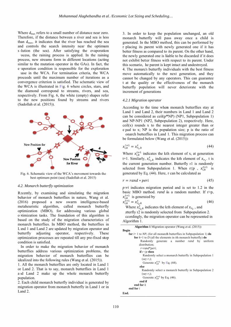
nd controls tolution (the rocess, the rarocess, new stmilar to the mvaporation conhase in the Wroceeds until onvergence cre WCA is illue diamond cspectively. Fr

the new pSadollah et al.

Fig. 6. Schematbest opti

2. Monarch b

ecently, by eehavior of mo016) proposetaheuristic

ptimization (ptimization taased on the sonarch butterand 1 and Lanutterfly adjuptimization prondition is satiIn order to mutterflies addrigration behealized into thAll the mona

r Land 2. Thand Land 2 mopulation.

Each child migration operaand 2.

New Position fNew Position f

Mo

ers to a small nhe distance bedicates that tthe search isea). After

aining procestreams form

mutation operndition is res

WCA. For terthe maximumiterion is satiustrated in Ficorrespond torom Fig. 6, thpositions fou(2015)).

tic view of the Wimum point (sea

utterfly optim

examining anonarch buttersed a new

algorithm, (MBO), for asks. The foustudy of the rflies. In MBnd 2 are updatusting operrocesses are reisfied. make the migress various

havior of mhe following rarch butterflieat is to say, mmake up the

monarch butterator from mon

for for

ohammad Ala

number of disetween a riverthe river has ntensity nearsatisfying t

s is applied. in different lator in the GAsponsible for rmination critm number ofsfied. The schig. 6 where cio streams, r

he white (empund by strea

WCA’s movema) (Sadollah et

ization

nd simulatingrflies in natur

swarm incalled monaddressing

undation of thmigration ch

O method, thted by migratiator, respecepeated till an

gration behavoptimization

monarch butterules (Wang etes are only lo

monarch buttee whole mo

rfly individualnarch butterfly

SSS

NNNeeewww PPPooosssiiitttiiiooonnn fffooorrr RRRiiivvveeerrr

aghebandha et

stance near zer and sea is lereached the sr the optimuthe evaporati

In the rainiocations (actiAs). In fact, tthe explorati

teria, the WCf iterations ashematic view ircles, stars, aivers, and s

pty) shapes reams and rive

ment towards theal. 2015)

g the migratire, Wang et telligence-bas

narch buttervarious glob

his algorithm haracteristics he butterflies ion operator actively. Theny pre-fixed st

vior of monar problems, terflies can t al. (2015)). cated in Landrflies in Land

onarch butter

l is generated y in Land 1 or

ddd

XXX

t al. /Economi

110

ero. ess sea um ion ing ing the ion CA s a of

and ea,

efer ers

he

ion al.

sed rfly bal

is of in

and ese top

rch the be

d 1 d 1 rfly

by r in

3.mgerebethnoth4.mcathbuin

4.

ALacaanceeqmbe

Wt+thsege

peba

buAA

Be

ic Lot Sizing a

In order to monarch butte

enerated. In theplacing its petter fitness ashe newly geneot exhibit betthis scenario, th The monarch

move automatannot be chanhat the qualitutterfly popuncrement of ge

2.1 Migration

According to tand 1 and Lanan be considend NP-NP1 (Neil(x) rounds qual to x; NP

monarch buttere formulated b

, ,

Where , ind+1. Similarly, he current genelected from enerated by Eq

eri indicates asic MBO me

, is generat

, , Where , inutterfly r2 is ra

Accordingly, thAlgorithm 1.

Algorithmegin for i= 1 to NP for k=1 to Rand

distrib r=ra if r ≤p Ra

(say Ge else

Ran(say

Ge end i end for k end for i

and Scheduling

keep the poerfly will pahe MBO metharent with ne

s compared to rated one is liter fitness withe parent is keh butterfly indically to the

nged by any oty or the ef

ulation will enerations

n operator

he time whennd 2, their nured as ceil(p*

NP2, Subpopux to the nea

P is the popuflies in Land

below (Wang

dicates the kt

, indicateneration numb

Subpopulatioq. (44). Here,

migration perethod. rand

i

ted by

ndicates the kandomly seleche migration o

m 1 Migration op

P1 (for all monarcho D (all the elemedomly generate bution; nd*peri; p then ndomly select a my r1); nerate , by E

ndomly select a my r2); nerate , by Eqf

g…

opulation uncass away onhod, this can bewly generate

o its parent. Oniable to be disth respect to iept intact and udividuals withe next generaoperators. Thiffectiveness onever deteri

n monarch buumbers in Lan*NP) (NP1, Sulation 2), resarest integer

ulation size; p1. This migraet al. (2015)):

th element ofes the kth elember. Butterflyon 1. When r can be calcu

riod and is sis a random

kth element ofcted from Suboperator can b

perator (Wang et

h butterflies in Suents in ith monarce a number

monarch butterfly

Eq. (44).

monarch butterfly

q. (46).

changed, an once a child be performed ed one if it hn the other hanscarded if it doits parent. Undundestroyed.

h the best fitnation, and this can guaranof the monariorate with

utterflies staynd 1 and LandSubpopulationspectively. Hegreater than

p is the ratio ation process c:

(4

f xi at generatiment of . t

y r1 is randomr≤p , ,

ulated as

(4

et to 1.2 in number. If r>

(4

f , and bpopulation 2e represented

al. (2015))

ubpopulation 1) dch butterfly) do rand by unifo

y in Subpopulatio

y in Subpopulatio

old is

by has nd, oes der

ess hey ntee rch the

y at d 2

n 1) ere,

or of

can

44)

ion t is

mly is

45)

the >p,

46)

2. in

do

form

on 1

on 2

End.


111

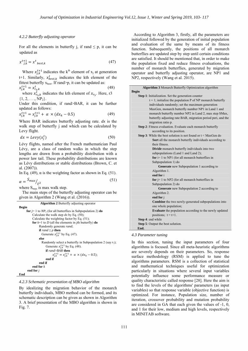
4.2.2 Butterfly adjusting operator

For all the elements in butterfly j, if rand ≤ p, it can be updated as

, , (47)

Where , indicates the kth element of xj at generation t+1. Similarly, , indicates the kth element of the fittest butterfly xbest. If rand>p, it can be updated as:

, , (48)

where , indicates the kth element of . Here, r3 � {1, 2, . . ., NP2}. Under this condition, if rand>BAR, it can be further updated as follows:

, , 0.5 (49)

Where BAR indicates butterfly adjusting rate. dx is the walk step of butterfly j and which can be calculated by Levy flight.

(50)

Lévy flights, named after the French mathematician Paul Lévy, are a class of random walks in which the step lengths are drawn from a probability distribution with a power law tail. These probability distributions are known as Lévy distributions or stable distributions (Brown, C. et al. (2007)). In Eq. (49), α is the weighting factor as shown in Eq. (51).

(51)

where Smax is max walk step. The main steps of the butterfly adjusting operator can be given in Algorithm 2 (Wang et al. (2016)).

Algorithm 2 Butterfly adjusting operator Begin for j= 1 to NP2 (for all butterflies in Subpopulation 2) do Calculate the walk step dx by Eq. (50); Calculate the weighting factor by Eq. (51); for k=1 to D (all the elements in jth butterfly) do Randomly generate rand; if rand ≤ p then Generate , by Eq. (47). else Randomly select a butterfly in Subpopulation 2 (say r3); Generate , by Eq. (48).

if rand>BAR then , , α 0.5 ; end if end if end for k end for j End

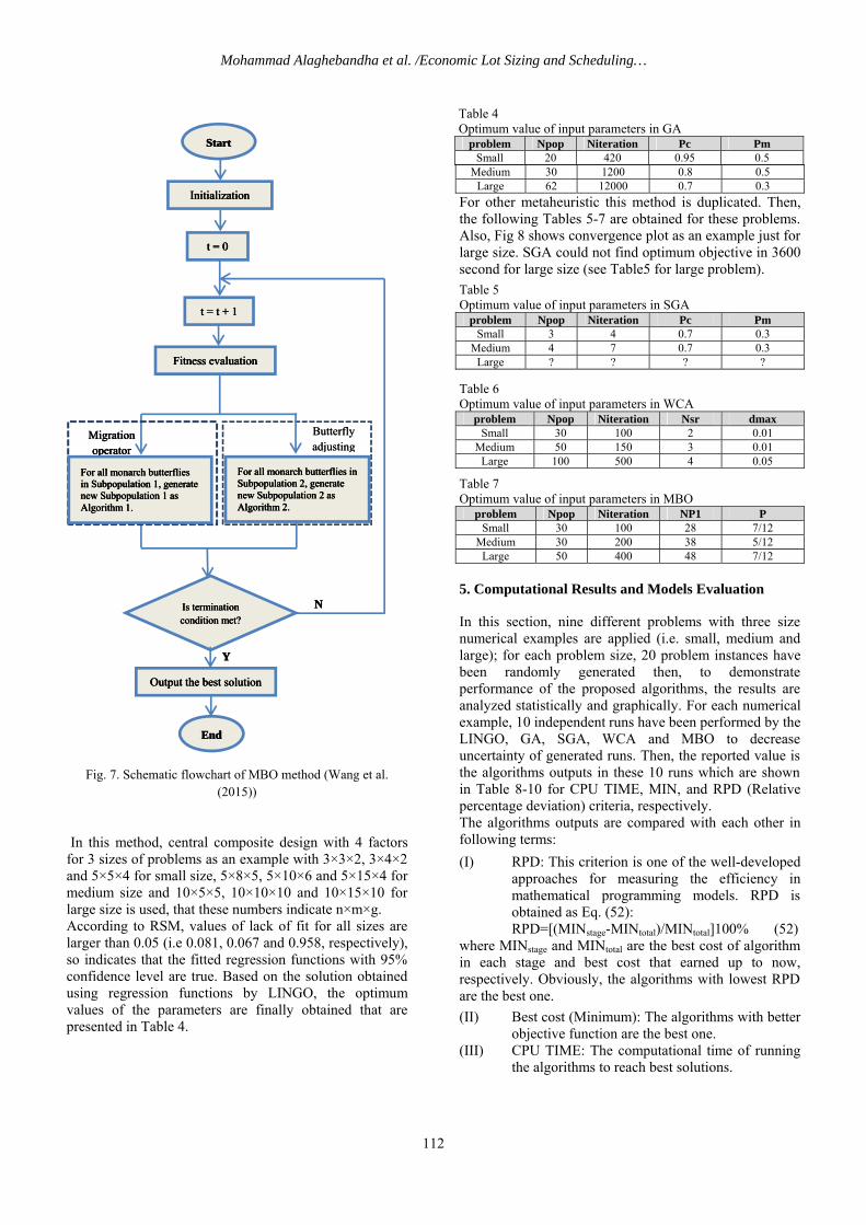
4.2.3 Schematic presentation of MBO algorithm

By idealizing the migration behavior of the monarch butterfly individuals, MBO method can be formed, and its schematic description can be given as shown in Algorithm 3. A brief presentation of the MBO algorithm is shown in Fig. 7.

According to Algorithm 3, firstly, all the parameters are initialized followed by the generation of initial population and evaluation of the same by means of its fitness function. Subsequently, the positions of all monarch butterflies are updated step by step until certain conditions are satisfied. It should be mentioned that, in order to make the population fixed and reduce fitness evaluations, the number of monarch butterflies, generated by migration operator and butterfly adjusting operator, are NP1 and NP2, respectively (Wang et al. 2015).

Algorithm 3 Monarch Butterfly Optimization algorithm Begin Step 1: Initialization. Set the generation counter

t = 1; initialize the population P of NP monarch butterfly individuals randomly; set the maximum generation MaxGen, monarch butterfly number NP1 in Land 1 and monarch butterfly number NP2 in Land 2, max step SMax, butterfly adjusting rate BAR, migration period peri, and the migration ratio p.

Step 2: Fitness evaluation. Evaluate each monarch butterfly according to its position.

Step 3: While the best solution is not found or t < MaxGen do Sort all the monarch butterfly individuals according to

their fitness. Divide monarch butterfly individuals into two

subpopulations (Land 1 and Land 2); for i= 1 to NP1 (for all monarch butterflies in

Subpopulation 1) do Generate new Subpopulation 1 according to

Algorithm 1. end for i for j= 1 to NP2 (for all monarch butterflies in

Subpopulation 2) do Generate new Subpopulation 2 according to

Algorithm 2. end for j Combine the two newly-generated subpopulations into

one whole population; Evaluate the population according to the newly updated

positions; t = t+1. Step 4: end while Step 5: Output the best solution.

End.

4.3 Parameter tuning

In this section, tuning the input parameters of four algorithms is focused. Since all meta-heuristic algorithms are severely depends on their parameters. So, response surface methodology (RSM) is applied to tune the algorithms parameters. RSM is a collection of statistical and mathematical techniques useful for optimization particularly in situations where several input variables potentially influence some performance measure or quality characteristic called response [28]. Here the aim is to find the levels of the algorithms' parameters (as input variables) so that response variable (objective function) is optimized. For instance, Population size, number of iteration, crossover probability and mutation probability are considered in GA that each given the values of -1, 0, and 1 for their low, medium and high levels, respectively in MINITAB software.


112

Fig. 7. Schematic flowchart of MBO method (Wang et al. (2015))

In this method, central composite design with 4 factors for 3 sizes of problems as an example with 3×3×2, 3×4×2 and 5×5×4 for small size, 5×8×5, 5×10×6 and 5×15×4 for medium size and 10×5×5, 10×10×10 and 10×15×10 for large size is used, that these numbers indicate n×m×g. According to RSM, values of lack of fit for all sizes are larger than 0.05 (i.e 0.081, 0.067 and 0.958, respectively), so indicates that the fitted regression functions with 95% confidence level are true. Based on the solution obtained using regression functions by LINGO, the optimum values of the parameters are finally obtained that are presented in Table 4.

0.5 0.8 1200 30 Medium 0.3 0.7 12000 62 Large

For other metaheuristic this method is duplicated. Then, the following Tables 5-7 are obtained for these problems. Also, Fig 8 shows convergence plot as an example just for large size. SGA could not find optimum objective in 3600 second for large size (see Table5 for large problem).

Table 5 Optimum value of input parameters in SGA

Pm Pc Niteration Npop problem0.3 0.7 4 3 Small 0.3 0.7 7 4 Medium ? ? ? ? Large

Table 6 Optimum value of input parameters in WCA

dmax Nsr Niteration Npop problem0.01 2 100 30 Small 0.01 3 150 50 Medium 0.05 4 500 100 Large

Table 7 Optimum value of input parameters in MBO

P NP1 Niteration Npop problem7/12 28 100 30 Small 5/12 38 200 30 Medium 7/12 48 400 50 Large

5. Computational Results and Models Evaluation

In this section, nine different problems with three size numerical examples are applied (i.e. small, medium and large); for each problem size, 20 problem instances have been randomly generated then, to demonstrate performance of the proposed algorithms, the results are analyzed statistically and graphically. For each numerical example, 10 independent runs have been performed by the LINGO, GA, SGA, WCA and MBO to decrease uncertainty of generated runs. Then, the reported value is the algorithms outputs in these 10 runs which are shown in Table 8-10 for CPU TIME, MIN, and RPD (Relative percentage deviation) criteria, respectively. The algorithms outputs are compared with each other in following terms:

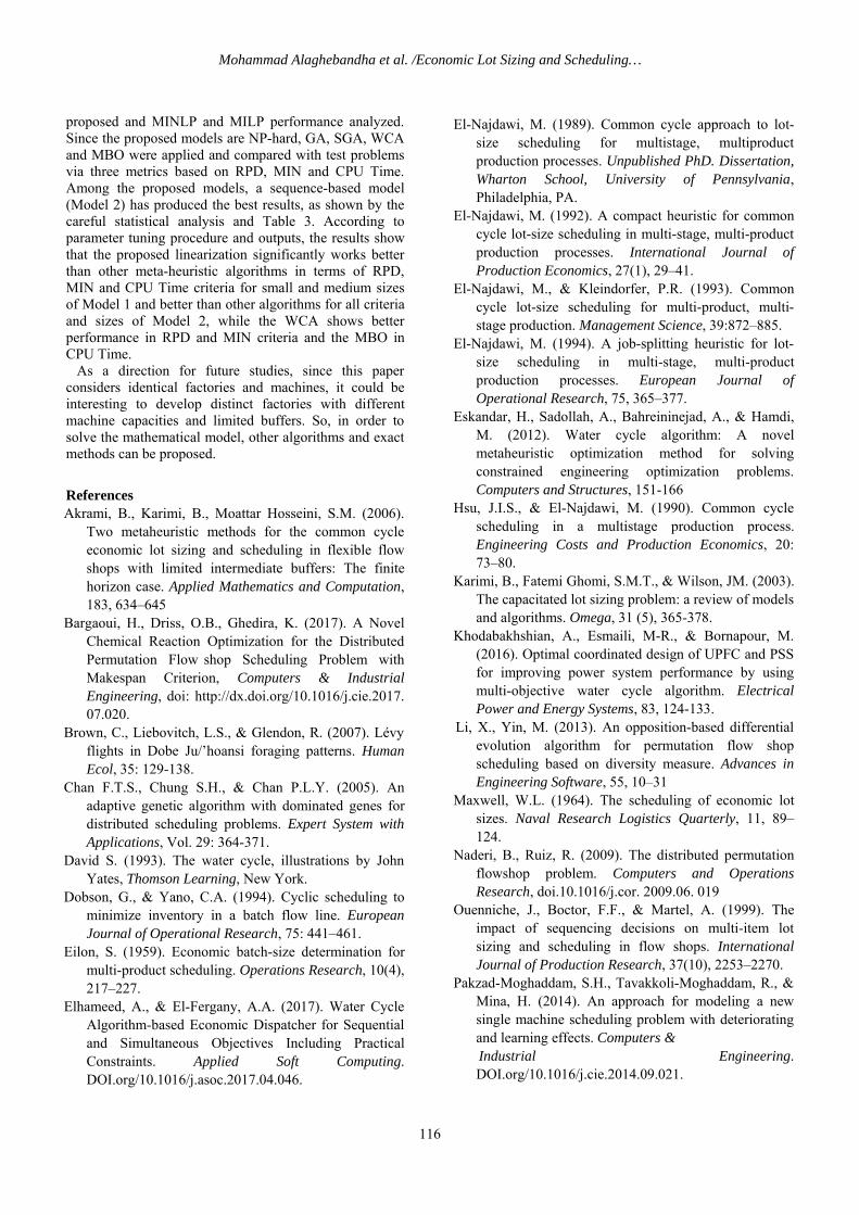
(I) RPD: This criterion is one of the well-developed approaches for measuring the efficiency in mathematical programming models. RPD is obtained as Eq. (52): RPD=[(MINstage-MINtotal)/MINtotal]100% (52)

where MINstage and MINtotal are the best cost of algorithm in each stage and best cost that earned up to now, respectively. Obviously, the algorithms with lowest RPD are the best one.

(II) Best cost (Minimum): The algorithms with better objective function are the best one.

(III) CPU TIME: The computational time of running the algorithms to reach best solutions.

MMMiiigggrrraaatttiiiooonnn ooopppeeerrraaatttooorrr

NNN

YYY

IIIsss ttteeerrrmmmiiinnnaaatttiiiooonnncccooonnndddiiitttiiiooonnn mmmeeettt???

Butterfly adjustingButterfly adjusting

OOOuuutttpppuuuttt ttthhheee bbbeeesssttt sssooollluuutttiiiooonnn

EEEnnnddd

IIInnniiitttiiiaaallliiizzzaaatttiiiooonnn

ttt === 000

ttt === ttt +++ 111

FFFiiitttnnneeessssss eeevvvaaallluuuaaatttiiiooonnn

SSStttaaarrrttt

FFFooorrr aaallllll mmmooonnnaaarrrccchhh bbbuuutttttteeerrrfffllliiieeesss iiinnn SSSuuubbbpppooopppuuulllaaatttiiiooonnn 222,,, gggeeennneeerrraaattteee nnneeewww SSSuuubbbpppooopppuuulllaaatttiiiooonnn 222 aaasss AAAlllgggooorrriiittthhhmmm 222...

FFFooorrr aaallllll mmmooonnnaaarrrccchhh bbbuuutttttteeerrrfffllliiieeesss iiinnn SSSuuubbbpppooopppuuulllaaatttiiiooonnn 111,,, gggeeennneeerrraaattteee nnneeewww SSSuuubbbpppooopppuuulllaaatttiiiooonnn 111 aaasss AAAlllgggooorrriiittthhhmmm 111...

Table 4 Optimum value of input parameters in GA

Pm Pc Niteration Npop problem0.5 0.95 420 20 Small

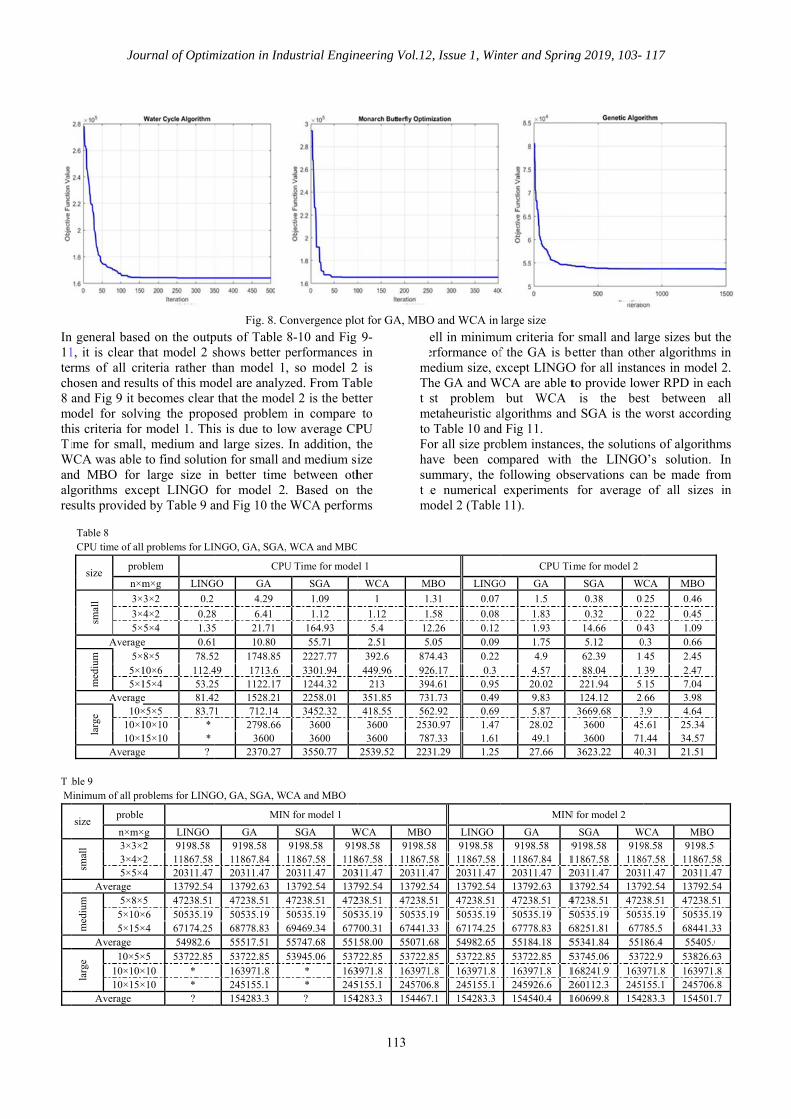
In11terch8 mothTiWanalgre

TaM

Jou

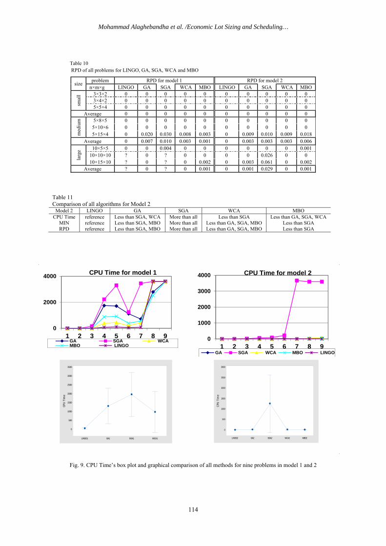
n general base1, it is clear thrms of all cri

hosen and resuand Fig 9 it bodel for solvis criteria for ime for small

WCA was able nd MBO for gorithms excsults provided

Table 8 CPU time of all

size prob

n×m

smal

l 3×

3×5×

Average

med

ium

5×5×15×1

Average

larg

e 10×10×110×1

Average

able 9 Minimum of all pro

size proble

n×m×

smal

l 3×3×23×4×25×5×4

Average

med

ium

5×8×5×10×5×15×

Average

larg

e 10×5×10×10×10×15×

Average

urnal of Optim

ed on the outphat model 2 siteria rather tults of this mobecomes clear ving the propo

model 1. Thi, medium andto find solutiolarge size in

ept LINGO d by Table 9 a

l problems for LIN

blem

m×g LING

3×2 0.2

4×2 0.285×4 1.35e 0.618×5 78.52

10×6 112.415×4 53.25e 81.42×5×5 83.710×10 * 15×10 * e ?

oblems for LING

em

×g LINGO 2 9198.58 2 11867.58 4 20311.47

13792.54 5 47238.51

×6 50535.19 ×4 67174.25

54982.6 ×5 53722.85 ×10 * ×10 *

?

mization in Ind

Fig. 8. C

puts of Table shows better pthan model 1odel are analyz

that the modeosed problemis is due to lod large sizes. on for small an better timefor model 2

and Fig 10 the

NGO, GA, SGA,

CPU

GO GA

4.29

8 6.41 5 21.71 1 10.80 2 1748.85

49 1713.6 5 1122.17 2 1528.21 1 712.14

2798.66 3600

2370.27

GO, GA, SGA, W

MIN

GA 9198.58

11867.84 20311.47 13792.63 47238.51 50535.19 68778.83 55517.51 53722.85 163971.8 245155.1 154283.3

dustrial Engin

Convergence plo

8-10 and Fig performances , so model 2zed. From Tabel 2 is the bet

m in compare ow average CP

In addition, tand medium si between oth. Based on t WCA perform

, WCA and MBO

U Time for mode

SGA

1.09

1.12 164.93 55.71

2227.77 3301.94 1244.32 2258.01 3452.32

3600 3600

3550.77

WCA and MBO

N for model 1

SGA W9198.58 91911867.58 11820311.47 20313792.54 13747238.51 47250535.19 50569469.34 67755747.68 55153945.06 537

* 163 * 245? 154

neering Vol.12

113

ot for GA, MBO

9- in

2 is ble tter

to PU the ize her the ms

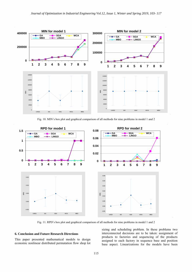
wpemThtemtoFohasuthm

O

el 1

WCA M

1 1

1.12 15.4 122.51 5

392.6 87449.96 92

213 39351.85 73418.55 563600 2533600 78

2539.52 223

WCA MBO98.58 9198.5

867.58 11867.311.47 20311.4792.54 13792.238.51 47238.535.19 50535.700.31 67441.158.00 55071.722.85 53722.3971.8 1639715155.1 2457064283.3 154467

2, Issue 1, Win

O and WCA in

well in minimuerformance of

medium size, ehe GA and Wst problem

metaheuristic ao Table 10 andor all size proave been comummary, the fhe numerical

model 2 (Table

MBO LINGO

.31 0.07

.58 0.082.26 0.12.05 0.094.43 0.226.17 0.34.61 0.951.73 0.49

62.92 0.6930.97 1.477.33 1.6131.29 1.25

O LINGO 58 9198.58 58 11867.5847 20311.4754 13792.5451 47238.5119 50535.1933 67174.2568 54982.6585 53722.851.8 163971.86.8 245155.17.1 154283.3

nter and Sprin

large size

um criteria forf the GA is bexcept LINGO

WCA are able tbut WCA

algorithms andd Fig 11. blem instancempared with following obsexperiments 11).

CPU Ti

O GA

1.5

1.83 1.93 1.75 4.9 4.57 20.02 9.83 5.87 28.02 49.1 27.66

MIN

GA 9198.58 911867.84 120311.47 213792.63 147238.51 450535.19 567778.83 655184.18 553722.85 5163971.8 1245926.6 2154540.4 1

ng 2019, 103-

r small and laetter than oth

O for all instanto provide low

is the besd SGA is the

es, the solutioh the LINGOservations canfor average

ime for model 2

SGA W

0.38 0.

0.32 0.14.66 0.5.12 0

62.39 1.88.04 1.221.94 5.124.12 2.3669.68 3

3600 453600 71

3623.22 40

N for model 2

SGA W9198.58 919

11867.58 118620311.47 203113792.54 137947238.51 472350535.19 505368251.81 67755341.84 55153745.06 537168241.9 1639260112.3 2451160699.8 1542

117

rge sizes but her algorithmsnces in modelwer RPD in east between worst accordi

ns of algorithO’s solution. n be made fro

of all sizes

CA MBO

25 0.46

22 0.45 43 1.09

0.3 0.66 45 2.45 39 2.47 15 7.04 66 3.98 .9 4.64 .61 25.34 .44 34.57

0.31 21.51

WCA MBO98.58 9198.5867.58 11867.511.47 20311.492.54 13792.538.51 47238.535.19 50535.1

785.5 68441.386.4 55405.0

722.9 53826.6971.8 163971.155.1 245706.283.3 154501.

the s in l 2. ach all

ing

hms In

om in

858 47 54 51 19 33 0

63 .8 .8 .7


114

Table 10 RPD of all problems for LINGO, GA, SGA, WCA and MBO

size problem RPD for model 1 RPD for model 2

n×m×g LINGO GA SGA WCA MBO LINGO GA SGA WCA MBO

smal

l 3×3×2 0 0 0 0 0 0 0 0 0 0 3×4×2 0 0 0 0 0 0 0 0 0 0 5×5×4 0 0 0 0 0 0 0 0 0 0

Average 0 0 0 0 0 0 0 0 0 0

med

ium

5×8×5 0 0 0 0 0 0 0 0 0 0 5×10×6 0 0 0 0 0 0 0 0 0 0 5×15×4 0 0.020 0.030 0.008 0.003 0 0.009 0.010 0.009 0.018

Average 0 0.007 0.010 0.003 0.001 0 0.003 0.003 0.003 0.006

larg

e 10×5×5 0 0 0.004 0 0 0 0 0 0 0.001 10×10×10 ? 0 ? 0 0 0 0 0.026 0 0 10×15×10 ? 0 ? 0 0.002 0 0.003 0.061 0 0.002

Average ? 0 ? 0 0.001 0 0.001 0.029 0 0.001

Table 11 Comparison of all algorithms for Model 2

Model 2 LINGO GA SGA WCA MBO CPU Time reference Less than SGA, WCA More than all Less than SGA Less than GA, SGA, WCA

MIN reference Less than SGA, MBO More than all Less than GA, SGA, MBO Less than SGA RPD reference Less than SGA, MBO More than all Less than GA, SGA, MBO Less than SGA

Fig. 9. CPU Time’s box plot and graphical comparison of all methods for nine problems in model 1 and 2

0

2000

4000

1 2 3 4 5 6 7 8 9

CPU Time for model 1

GA SGA WCAMBO LINGO

0

1000

2000

3000

4000

1 2 3 4 5 6 7 8 9

CPU Time for model 2

GA SGA WCA MBO LINGO

WCA1SGA1GA1LINGO1

3500

3000

2500

2000

1500

1000

500

0

CPU

Tim

e

MBO2WCA2SGA2GA2LINGO2

3000

2500

2000

1500

1000

500

0

CPU

Tim

e


115

Fig. 10. MIN’s box plot and graphical comparison of all methods for nine problems in model 1 and 2

Fig. 11. RPD’s box plot and graphical comparison of all methods for nine problems in model 1 and 2

6. Conclusion and Future Research Directions

This paper presented mathematical models to design economic nonlinear distributed permutation flow shop lot

sizing and scheduling problem. In these problems two interconnected decisions are to be taken: assignment of products to factories and sequencing of the products assigned to each factory in sequence base and position base aspect. Linearizations for the models have been

0

200000

400000

1 2 3 4 5 6 7 8 9

MIN for model 1 GA SGA WCAMBO LINGO

0

100000

200000

300000

1 2 3 4 5 6 7 8 9

MIN for model 2

GA SGA WCAMBO LINGO


140000

120000

100000

80000

60000

40000

20000

0

MIN


140000

120000

100000

80000

60000

40000

20000

0

MIN

0

0.5

1

1.5

1 2 3 4 5 6 7 8 9

RPD for model 1

GA SGA WCAMBO LINGO

0

0.02

0.04

0.06

0.08

1 2 3 4 5 6 7 8 9

RPD for model 2

GA SGA WCAMBO LINGO


0.015

0.010

0.005

0.000

-0.005

RPD


0.030

0.025

0.020

0.015

0.010

0.005

0.000

-0.005

RPD


116

proposed and MINLP and MILP performance analyzed. Since the proposed models are NP-hard, GA, SGA, WCA and MBO were applied and compared with test problems via three metrics based on RPD, MIN and CPU Time. Among the proposed models, a sequence-based model (Model 2) has produced the best results, as shown by the careful statistical analysis and Table 3. According to parameter tuning procedure and outputs, the results show that the proposed linearization significantly works better than other meta-heuristic algorithms in terms of RPD, MIN and CPU Time criteria for small and medium sizes of Model 1 and better than other algorithms for all criteria and sizes of Model 2, while the WCA shows better performance in RPD and MIN criteria and the MBO in CPU Time.

As a direction for future studies, since this paper considers identical factories and machines, it could be interesting to develop distinct factories with different machine capacities and limited buffers. So, in order to solve the mathematical model, other algorithms and exact methods can be proposed.

References Akrami, B., Karimi, B., Moattar Hosseini, S.M. (2006).

Two metaheuristic methods for the common cycle economic lot sizing and scheduling in flexible flow shops with limited intermediate buffers: The finite horizon case. Applied Mathematics and Computation, 183, 634–645

Bargaoui, H., Driss, O.B., Ghedira, K. (2017). A Novel Chemical Reaction Optimization for the Distributed Permutation Flow shop Scheduling Problem with Makespan Criterion, Computers & Industrial Engineering, doi: http://dx.doi.org/10.1016/j.cie.2017. 07.020.

Brown, C., Liebovitch, L.S., & Glendon, R. (2007). Lévy flights in Dobe Ju/’hoansi foraging patterns. Human Ecol, 35: 129-138.

Chan F.T.S., Chung S.H., & Chan P.L.Y. (2005). An adaptive genetic algorithm with dominated genes for distributed scheduling problems. Expert System with Applications, Vol. 29: 364-371.

David S. (1993). The water cycle, illustrations by John Yates, Thomson Learning, New York.

Dobson, G., & Yano, C.A. (1994). Cyclic scheduling to minimize inventory in a batch flow line. European Journal of Operational Research, 75: 441–461.

Eilon, S. (1959). Economic batch-size determination for multi-product scheduling. Operations Research, 10(4), 217–227.

Elhameed, A., & El-Fergany, A.A. (2017). Water Cycle Algorithm-based Economic Dispatcher for Sequential and Simultaneous Objectives Including Practical Constraints. Applied Soft Computing. DOI.org/10.1016/j.asoc.2017.04.046.

El-Najdawi, M. (1989). Common cycle approach to lot-size scheduling for multistage, multiproduct production processes. Unpublished PhD. Dissertation, Wharton School, University of Pennsylvania, Philadelphia, PA.

El-Najdawi, M. (1992). A compact heuristic for common cycle lot-size scheduling in multi-stage, multi-product production processes. International Journal of Production Economics, 27(1), 29–41.

El-Najdawi, M., & Kleindorfer, P.R. (1993). Common cycle lot-size scheduling for multi-product, multi-stage production. Management Science, 39:872–885.

El-Najdawi, M. (1994). A job-splitting heuristic for lot-size scheduling in multi-stage, multi-product production processes. European Journal of Operational Research, 75, 365–377.

Eskandar, H., Sadollah, A., Bahreininejad, A., & Hamdi, M. (2012). Water cycle algorithm: A novel metaheuristic optimization method for solving constrained engineering optimization problems. Computers and Structures, 151-166

Hsu, J.I.S., & El-Najdawi, M. (1990). Common cycle scheduling in a multistage production process. Engineering Costs and Production Economics, 20: 73–80.

Karimi, B., Fatemi Ghomi, S.M.T., & Wilson, JM. (2003). The capacitated lot sizing problem: a review of models and algorithms. Omega, 31 (5), 365-378.

Khodabakhshian, A., Esmaili, M-R., & Bornapour, M. (2016). Optimal coordinated design of UPFC and PSS for improving power system performance by using multi-objective water cycle algorithm. Electrical Power and Energy Systems, 83, 124-133.

Li, X., Yin, M. (2013). An opposition-based differential evolution algorithm for permutation flow shop scheduling based on diversity measure. Advances in Engineering Software, 55, 10–31

Maxwell, W.L. (1964). The scheduling of economic lot sizes. Naval Research Logistics Quarterly, 11, 89–124.

Naderi, B., Ruiz, R. (2009). The distributed permutation flowshop problem. Computers and Operations Research, doi.10.1016/j.cor. 2009.06. 019

Ouenniche, J., Boctor, F.F., & Martel, A. (1999). The impact of sequencing decisions on multi-item lot sizing and scheduling in flow shops. International Journal of Production Research, 37(10), 2253–2270.

Pakzad-Moghaddam, S.H., Tavakkoli-Moghaddam, R., & Mina, H. (2014). An approach for modeling a new single machine scheduling problem with deteriorating and learning effects. Computers &

Industrial Engineering.DOI.org/10.1016/j.cie.2014.09.021.

Ra

Ri

Ro

Ro

Sa

Sa

Th S

Jo

httDO

Jou

ahman, H.F., Algorithm under MakeIndustrial 10.1016/j.ci

fai, A. P., Ngobjective adistributed scheduling.

odriguez, M.AGrossmann,and managedemand uncComputers a

ogers, J. (19economic Science, 4(3

adollah, A., EsH. (2015). rate for soptimization48-51.

adollah, A., E(2015). Appdifferential function anApplications

his article canizing and Schournal of Opti

tp://www.qjieOI: 10.22094/

urnal of Optim

Sarker, R., Efor Permutat

e to Stock ProdEngineering

ie.2015.08.006guyen, H.T., &adaptive large

reentrant Applied Soft C

A., Vecchiett, I.E. (2014). ement over acertainty. Part and Chemical

958). A comlot scheduli

3), 264–291. skandar, H., BWater cycle

solving consn problems.

Eskandar, H.proximate so

equations und metaheuriss of Artificial

n be cited: Alheduling in Diimization in In

e.ir/article_543/JOIE.2018.54

mization in Ind

Essam, D. (20tion Flow Shduction systemg, doi: h6 & Dawal, S.Z

e Neighborhopermutation

Computing, 40ti, A.R., HarjOptimal supp

a multi-periodI: MINLP and

l Engineering,mputational aping problem

Bahreininejadalgorithm w

strained and Applied Soft

, Yoo, D-G.olving of nonusing least stic algorithmIntelligence, 4

laghebandha Mstributed Permndustrial Eng

3808.html 42997.1510

dustrial Engin

015). A Genehop Schedulim. Computershttp://dx.doi.or

Z. (2016). Mulood search f

flow sh0, 42–57. rjunkoski, I., ply chain desid horizon undd MILP mode, 62, 194–210pproach to t

m. Manageme

d, A., & Kim,with evaporati

unconstrainComputing, 3

, & Kim, J-nlinear ordina

square weigms., Engineeri

40: 117-132.

M., Naderi B.mutation Flowgineering. 12 (

neering Vol.12

117

etic ing s & rg/

lti-for

hop

& ign der els. 0. the ent

, J-ion ned 30:

-H. ary ght ing

To

Yo

V

W

W

W

W

& Mohammaw Shops. (1), 103- 117.

2, Issue 1, Win

orabi, S.A., (2005). Theflexible joInternationa52–65.

ou, F., & GEchelon SuUncertaintyStrategies, C

Viagas, V.F., Gdistributed total flow ti118, 464–47

Wang, B. (19enterprise d

Wang, G-G., Dmonarch bcrossover 10.1007/s12

Wang, G-G., Deoptimizations00521-015

Wang, G-G., ZMonarch Buand Self-internationaintelligenceDOI 10.110

adi M. (2019)

nter and Sprin

Karimi, B., e common cycob shops: al Journal of

rossmann, I.Epply Chain D

y: MINLP Carnegie Mell

Gonzalez, P.P.permutation

ime. Compute77. 997). Integraesign. Chapmeb, S., Zhao, utterfly optimoperator. O

2351-016-025eb, S., & Cui,n. Neural Com-1923-y. Zhao, X., &utterfly Optim

f-adaptive Cal conference , Hong Kong

09/ISCMI.201

. Economic Lo

ng 2019, 103-

& Fatemi cle economic lThe finite f Production

E. (2008). InDesign with In

Models. lon University, Framinan, Jflow shop t

ers & Industr

ated productman and Hall,

X., & Cui, Zmization withOper Res

51-z , Z. (2015). Mmput & Appli

& Deb, S. (2mization with Crossover on soft compu

g, (ISCMI 2015.19

ot

117

Ghomi, S.Mlot scheduling

horizon caEconomics,

ntegrated Munventories und

Computationy, USA. . M. (2018). Tto minimise rial Engineerin

t, process a1st Edition,

Z. (2016). A nh an improv

Int J. D

Monarch butteric. DOI:10.100

2015). A NoGreedy StrateOperator, uting & mach15),

Nov 23–2

M.T. g in ase. 97,

ulti-der nal

The the ng,

and

new ved

DOI

rfly 07/

vel egy 2nd

ine 24.

Documents

Economic Lot Sizing and Scheduling in Distributed