Embed Size (px)
Citation preview

Institute of Engineering, Surveyingand Space Geodesy
Heave Compensation UsingTime-Differenced Carrier Observations
from Low Cost GPS Receivers
By
Stephen J. Blake BEng
Thesis submitted to the University of Nottingham forthe degree of Doctor of Philosophy
June 2007

i
ABSTRACT
Vertical reference for hydrographic survey can be provided in two ways: through the
use of an expensive and very accurate GPS-aided INS system, or through the classical
method of compensating for heave motion measured on board the vessel and tide data
taken from a nearby tide gauge. Whilst the GPS-aided INS approach offers significant
advantages in terms of accuracy their high cost has prohibited their widespread use
within the hydrographic survey industry and the classical method is still prevalent.
Heave motion of a survey vessel has traditionally been measured using inertial
technologies, which can be expensive and have problems with usability and instability,
resulting in higher survey costs and a significant hydrographer input burden. Heave
can also be measured through the use GPS receivers by the differencing of measured
carrier phase pseudo-range from adjacent epochs and the recent introduction by
U-Blox of the Antaris AEK-4T, an off the shelf low cost GPS receiver capable of
measuring and recording the carrier phase pseudo-range observable, has allowed the
exploration of a novel method of measuring and compensating for vessel heave using
off the shelf low cost GPS receivers.
The work presented in this thesis details a method of compensating for vessel heave
motion in bathymetry data that has been developed specifically for use with the
U-Blox Antaris receiver. The technique is based on the production of highly accurate
velocity estimates using the carrier phase observable. Carrier phase measurements
are differenced across adjacent epochs to give relative delta range estimates between
receiver and satellite along the direct line of sight, which are then processed to calcu-
late an accurate estimate of receiver delta position across the epoch, a measurement
analogous to receiver velocity. This technique has been termed Temporal Double
Differencing (TDD).
Integrated vertical velocity estimates produce the relative vertical displacement of
the vessel over time. Because of bias errors in the velocity estimates from TDD, this
vertical displacement is subject to drift. The drift is removed by passing the data
through a high-pass filter designed to stop the drift frequencies yet pass the required
frequencies of vertical vessel motion.

ii
An obvious advantage of this technique over conventional technologies is cost.
Instruments currently on the market are centred on inertial sensors and generally
have prices ranging from £12,000 to £25,000. Low cost GPS receivers are priced
at around £200 and so this technique can have sizeable cost implications for the
hydrographic survey industry. In addition the nature of the TDD algorithm results
in a heave sensing technology that is not subject to turn induced heave which can
affect inertial based sensors, and also imposes no requirement on the user to account
for parameters such as vessel heave characteristics and current heave state. A further
advantage over interferometric GPS heave compensation techniques is that the TDD
algorithm is stand-alone and requires no reference receiver.
Two trials have been undertaken to test the ability of the low cost U-Blox receiver
to record accurate phase pseudo-range observables and subsequently produce a heave
estimate: a Spirent GPS hardware simulator trial, and a sea trial. The simulator trial
has been the first to quantify the errors associated with the measurement of carrier
phase pseudo-range observables using low cost commercially available receivers. The
trial used three separate receivers: a Novatel OEM4, a Leica 530 and a low cost U-
Blox Antaris. Three scenarios were programmed into the simulator to rigorously test
the effects of receiver quality and receiver dynamics on the resulting velocity estimates
using the TDD algorithm. The sea trial involved fitting various sensors to the vessel
including a Honeywell HG1700 IMU, an Applanix POS-RS GPS-aided INS system
and the same three GPS receivers as used in the simulator trial. The POS-RS system
and the inertial based heave sensor were used to provide a reference against which the
novel low cost heave output could be compared. The comprehensive nature of the sea
trial makes it the first work to compare the results from the TDD heave algorithm
using varying grades of receiver, and against truth data from both an inertial based
heave system and a GPS-aided INS.
The results of the simulator trial have shown that under static conditions the
TDD velocity estimation using the U-Blox Antaris is of comparable quality to that
produced using both the Novatel OEM4 and the Leica 530. Under dynamic conditions
the performance of the U-Blox Antaris is greatly degraded when undergoing large
accelerations, an artefact of the inferior componentry used in the signal tracking loops.

iii
The sea trial has demonstrated the ability of the TDD heave algorithm developed for
use with commercially available low cost GPS receivers to measure vessel heave to
a similar standard as inertial based technologies at a fraction of the cost and with
greatly reduced instability and usability issues that are traditionally associated with
inertial based heave sensors.

iv
Acknowledgements
This PhD project has been undertaken at the Institute of Engineering Surveying and
Space Geodesy, University of Nottingham in conjunction with Sonardyne Interna-
tional Limited. Funding for the project has been supplied by both the EPSRC, and
Sonardyne International Limited through an Industrial CASE award.
I would like to extend my thanks to all those who have aided me as I conducted
the research for the project with particular thanks to my academic supervisors: Prof.
Terry Moore, Dr. Chris Hide, Dr. David Park and Dr. Chris Hill. I would also like to
thank Sonardyne International Ltd. and my industrial supervisors there: Jonathan
Martin and Chris Pearce.

Contents
1 Introduction 1
1.1 Background . . . . . . . . . . . . . . . . . . . . . . . . . . . . . . . . 1
1.2 Research Aims and Objectives . . . . . . . . . . . . . . . . . . . . . . 3
1.3 Research Methodology . . . . . . . . . . . . . . . . . . . . . . . . . . 4
1.4 Thesis Overview . . . . . . . . . . . . . . . . . . . . . . . . . . . . . . 5
2 Inertial Navigation Systems 8
2.1 Introduction . . . . . . . . . . . . . . . . . . . . . . . . . . . . . . . . 8
2.2 The Principles of Inertial Navigation . . . . . . . . . . . . . . . . . . 9
2.2.1 Reference Frames . . . . . . . . . . . . . . . . . . . . . . . . . 9
2.2.2 Frame Rotations . . . . . . . . . . . . . . . . . . . . . . . . . 12
2.2.2.1 Euler Angles . . . . . . . . . . . . . . . . . . . . . . 13
2.2.2.2 Quaternions . . . . . . . . . . . . . . . . . . . . . . . 14
2.2.3 The Strapdown Inertial Navigation Concept . . . . . . . . . . 17
2.3 System Initialization and Alignment . . . . . . . . . . . . . . . . . . . 18
2.3.1 Initialization . . . . . . . . . . . . . . . . . . . . . . . . . . . . 18
2.3.2 Alignment . . . . . . . . . . . . . . . . . . . . . . . . . . . . . 18
2.3.2.1 Coarse Alignment . . . . . . . . . . . . . . . . . . . 19
2.3.2.2 Fine Alignment . . . . . . . . . . . . . . . . . . . . . 21
2.4 System Mechanisation in the Navigation Frame . . . . . . . . . . . . 22
2.5 Attitude and Heading Reference Systems . . . . . . . . . . . . . . . . 24
2.5.1 AHRS Alignment and Operation . . . . . . . . . . . . . . . . 25
2.6 Grades of IMU . . . . . . . . . . . . . . . . . . . . . . . . . . . . . . 27
v

Contents vi
3 The Global Positioning System 30
3.1 Introduction . . . . . . . . . . . . . . . . . . . . . . . . . . . . . . . . 30
3.2 GPS Overview . . . . . . . . . . . . . . . . . . . . . . . . . . . . . . . 31
3.2.1 The Basic Concept . . . . . . . . . . . . . . . . . . . . . . . . 31
3.2.2 GPS Hardware . . . . . . . . . . . . . . . . . . . . . . . . . . 31
3.2.2.1 The Space Segment . . . . . . . . . . . . . . . . . . . 32
3.2.2.2 The Control Segment . . . . . . . . . . . . . . . . . . 33
3.2.2.3 The User Segment . . . . . . . . . . . . . . . . . . . 33
3.3 GPS Observables . . . . . . . . . . . . . . . . . . . . . . . . . . . . . 34
3.3.1 The Code Pseudo-range Observable . . . . . . . . . . . . . . . 34
3.3.2 The Carrier Phase Pseudo-range Observable . . . . . . . . . . 37
3.3.3 The Pseudo-range Rate Observable . . . . . . . . . . . . . . . 37
3.3.4 Quality of Recorded Observables . . . . . . . . . . . . . . . . 38
3.3.4.1 Signal Tracking with Feedback Control Loops . . . . 38
3.3.4.2 Feedback Control Loop Performance . . . . . . . . . 39
3.4 GPS Error Sources . . . . . . . . . . . . . . . . . . . . . . . . . . . . 41
3.4.1 Satellite Errors . . . . . . . . . . . . . . . . . . . . . . . . . . 42
3.4.1.1 Satellite Clock Offset . . . . . . . . . . . . . . . . . . 42
3.4.1.2 Ephemeris Error . . . . . . . . . . . . . . . . . . . . 42
3.4.2 Measurement Errors . . . . . . . . . . . . . . . . . . . . . . . 43
3.4.2.1 Receiver Clock Offset . . . . . . . . . . . . . . . . . 43
3.4.2.2 Multipath Error . . . . . . . . . . . . . . . . . . . . 44
3.4.2.3 Receiver Noise and Tracking Loop Errors . . . . . . 44
3.4.3 Propagation Errors . . . . . . . . . . . . . . . . . . . . . . . . 44
3.4.3.1 Ionospheric Effects . . . . . . . . . . . . . . . . . . . 45
3.4.3.2 Tropospheric Delay . . . . . . . . . . . . . . . . . . . 46
3.5 Obtaining User Position from GPS Observables . . . . . . . . . . . . 47
3.5.1 Stand-alone GPS . . . . . . . . . . . . . . . . . . . . . . . . . 48
3.5.2 Differential Positioning . . . . . . . . . . . . . . . . . . . . . . 52
3.5.3 Interferometric Positioning . . . . . . . . . . . . . . . . . . . . 53
3.5.3.1 Single Difference . . . . . . . . . . . . . . . . . . . . 53

Contents vii
3.5.3.2 Double Difference . . . . . . . . . . . . . . . . . . . . 54
3.5.4 Spacial Decorrelation . . . . . . . . . . . . . . . . . . . . . . . 54
3.6 Obtaining User Velocity from a Stand-alone GPS Receiver . . . . . . 55
3.6.1 Velocity from the Pseudo-range Rate Observable . . . . . . . . 56
3.6.2 Velocity from Temporally Differenced Carrier Phase Observables 57
4 Vertical Reference for Hydrographic Survey 58
4.1 Introduction . . . . . . . . . . . . . . . . . . . . . . . . . . . . . . . . 58
4.2 Chart Datum . . . . . . . . . . . . . . . . . . . . . . . . . . . . . . . 59
4.3 Classical Hydrographic Methods . . . . . . . . . . . . . . . . . . . . . 60
4.3.1 Tidal Compensation . . . . . . . . . . . . . . . . . . . . . . . 60
4.3.2 Heave Compensation . . . . . . . . . . . . . . . . . . . . . . . 62
4.3.2.1 Analogue Heave Reduction . . . . . . . . . . . . . . 63
4.3.2.2 Digital Heave Compensation . . . . . . . . . . . . . . 63
4.3.3 Errors and Problems Associated with Classical Hydrographic
Methods . . . . . . . . . . . . . . . . . . . . . . . . . . . . . . 65
4.3.3.1 Tide Specific Errors . . . . . . . . . . . . . . . . . . 65
4.3.3.2 Heave Specific Errors . . . . . . . . . . . . . . . . . . 66
4.3.3.3 General Classical Methodology Errors . . . . . . . . 67
4.4 Single Water Level Correction . . . . . . . . . . . . . . . . . . . . . . 68
4.4.1 GPS-aided INS . . . . . . . . . . . . . . . . . . . . . . . . . . 68
4.4.2 Interferometric GPS . . . . . . . . . . . . . . . . . . . . . . . 70
4.4.3 Factors Prohibitive to the Widespread Use of Single Water Level
Correction Techniques . . . . . . . . . . . . . . . . . . . . . . 70
4.4.3.1 GPS-aided INS Specific Factors . . . . . . . . . . . . 70
4.4.3.2 Interferometric GPS Specific Factors . . . . . . . . . 71
4.4.3.3 General Single Water Level Correction Methodology
Factors . . . . . . . . . . . . . . . . . . . . . . . . . 71
4.5 The International Hydrographic Organization Survey Standards . . . 72
5 Development of an INS Based Heave Algorithm 74
5.1 Introduction . . . . . . . . . . . . . . . . . . . . . . . . . . . . . . . . 74

Contents viii
5.2 INS Mechanisation . . . . . . . . . . . . . . . . . . . . . . . . . . . . 75
5.2.1 Initialization and Alignment . . . . . . . . . . . . . . . . . . . 75
5.2.2 The INS Mechanisation Computation Loop . . . . . . . . . . . 76
5.2.2.1 Earth and Transport Rate . . . . . . . . . . . . . . . 76
5.2.2.2 Gravity Compensation . . . . . . . . . . . . . . . . . 77
5.2.2.3 Formation of the Navigation Frame Mechanisation Equa-
tion . . . . . . . . . . . . . . . . . . . . . . . . . . . 77
5.2.2.4 Velocity and Position Updates . . . . . . . . . . . . . 78
5.2.2.5 Attitude Computation . . . . . . . . . . . . . . . . . 78
5.2.2.6 Subsequent Loop Iterations . . . . . . . . . . . . . . 79
5.2.3 Fourth Order Runge-Kutta Numerical Integration . . . . . . . 79
5.3 INS Vertical Channel Damping . . . . . . . . . . . . . . . . . . . . . 80
5.3.1 The Baro-inertial Altimeter . . . . . . . . . . . . . . . . . . . 81
5.3.1.1 A Heave Filter Based on the Baro-inertial Altimeter 82
5.3.1.2 Frequency and Transient Analysis of the Baro-inertial
Altimeter Based Heave Filter . . . . . . . . . . . . . 83
5.3.1.3 Redesign of the Heave Filter to Incorporate a Damping
Coefficient . . . . . . . . . . . . . . . . . . . . . . . . 84
5.3.1.4 Transient Analysis of the Redesigned Heave Filter . . 86
5.3.2 Heave Filter Tuning . . . . . . . . . . . . . . . . . . . . . . . 86
5.4 Use of Inertial Based Heave Algorithms in Hydrographic Survey . . . 88
5.4.1 Summary of Inertial Heave Algorithm . . . . . . . . . . . . . . 88
5.4.2 Turn Induced Heave and Filter Transient Behaviour . . . . . . 89
5.4.3 Heave Filter Tuning . . . . . . . . . . . . . . . . . . . . . . . 90
5.4.4 Cost Implications of Inertial Heave Systems . . . . . . . . . . 90
6 Development of a GPS Velocity Based Heave Algorithm 92
6.1 Introduction . . . . . . . . . . . . . . . . . . . . . . . . . . . . . . . . 92
6.2 Velocity From Time-Differenced Carrier Phase Pseudo-range . . . . . 93
6.2.1 The Temporal Double Difference Observation Equation . . . . 93
6.2.2 The TDD Processing Algorithm . . . . . . . . . . . . . . . . . 94

Contents ix
6.2.3 Specific Models and Techniques Used in the TDD Velocity Al-
gorithm . . . . . . . . . . . . . . . . . . . . . . . . . . . . . . 97
6.2.3.1 Satellite Ephemeris Calculation . . . . . . . . . . . . 97
6.2.3.2 Stand-alone GPS Position . . . . . . . . . . . . . . . 98
6.2.3.3 Tropospheric Correction . . . . . . . . . . . . . . . . 98
6.2.3.4 Ionospheric Correction . . . . . . . . . . . . . . . . . 100
6.2.3.5 Correction for Satellite Loss . . . . . . . . . . . . . . 102
6.2.3.6 Cycle Slip Handling . . . . . . . . . . . . . . . . . . 103
6.2.3.7 Carrier-to-Noise Density Weighting Scheme . . . . . 104
6.3 The TDD Heave Algorithm . . . . . . . . . . . . . . . . . . . . . . . 105
7 The Spirent GSS7700 GPS/SBAS Simulator Trials 108
7.1 Introduction . . . . . . . . . . . . . . . . . . . . . . . . . . . . . . . . 108
7.2 The Spirent GSS7700 GPS/SBAS Simulator . . . . . . . . . . . . . . 109
7.2.1 Simulator Hardware . . . . . . . . . . . . . . . . . . . . . . . 109
7.2.2 Simulator Software . . . . . . . . . . . . . . . . . . . . . . . . 110
7.2.3 Simulator Setup and Error Models . . . . . . . . . . . . . . . 110
7.3 Trial Methodology . . . . . . . . . . . . . . . . . . . . . . . . . . . . 111
7.3.1 The Simulated Scenarios . . . . . . . . . . . . . . . . . . . . . 112
7.3.1.1 Static . . . . . . . . . . . . . . . . . . . . . . . . . . 112
7.3.1.2 Marine . . . . . . . . . . . . . . . . . . . . . . . . . . 113
7.3.1.3 High Dynamics . . . . . . . . . . . . . . . . . . . . . 115
7.3.2 The Trials . . . . . . . . . . . . . . . . . . . . . . . . . . . . . 115
7.3.2.1 Trial 1: Receiver Test . . . . . . . . . . . . . . . . . 117
7.3.2.2 Trial 2: Tropospheric Delay Compensation Test . . . 118
7.3.2.3 Trial 3: Ionospheric Delay Compensation Test . . . . 118
7.3.2.4 Trial 4: Full Simulation Test . . . . . . . . . . . . . . 118
7.3.2.5 Trial 5: Real Static Data . . . . . . . . . . . . . . . . 119
7.4 Trial Results . . . . . . . . . . . . . . . . . . . . . . . . . . . . . . . . 119
7.4.1 Trial 1 . . . . . . . . . . . . . . . . . . . . . . . . . . . . . . . 119
7.4.1.1 Static Scenario . . . . . . . . . . . . . . . . . . . . . 119

Contents x
7.4.1.2 Marine Scenario . . . . . . . . . . . . . . . . . . . . 120
7.4.1.3 High Dynamic Scenario . . . . . . . . . . . . . . . . 127
7.4.2 Trial 2 . . . . . . . . . . . . . . . . . . . . . . . . . . . . . . . 131
7.4.3 Trial 3 . . . . . . . . . . . . . . . . . . . . . . . . . . . . . . . 133
7.4.4 Trial 4 . . . . . . . . . . . . . . . . . . . . . . . . . . . . . . . 134
7.4.5 Trial 5 . . . . . . . . . . . . . . . . . . . . . . . . . . . . . . . 137
7.5 Spirent Simulator Trial Summary . . . . . . . . . . . . . . . . . . . . 137
8 The Plymouth Sea Trial 142
8.1 Introduction . . . . . . . . . . . . . . . . . . . . . . . . . . . . . . . . 142
8.2 Trial Methodology . . . . . . . . . . . . . . . . . . . . . . . . . . . . 143
8.2.1 Trial Overview . . . . . . . . . . . . . . . . . . . . . . . . . . 143
8.2.2 The Applanix POSRS System . . . . . . . . . . . . . . . . . . 144
8.2.3 The Marco and the Sensor Configuration . . . . . . . . . . . . 144
8.2.4 Trial Trajectory . . . . . . . . . . . . . . . . . . . . . . . . . . 146
8.2.5 Vessel Reference Point and Lever Arm Separations . . . . . . 150
8.3 Trial Results . . . . . . . . . . . . . . . . . . . . . . . . . . . . . . . . 152
8.3.1 POSRS SBET Data . . . . . . . . . . . . . . . . . . . . . . . 152
8.3.1.1 SBET Data Quality . . . . . . . . . . . . . . . . . . 152
8.3.1.2 SBET Heave . . . . . . . . . . . . . . . . . . . . . . 155
8.3.2 IMU Derived Heave . . . . . . . . . . . . . . . . . . . . . . . . 157
8.3.3 TDD Heave . . . . . . . . . . . . . . . . . . . . . . . . . . . . 160
8.3.3.1 Leica 530 Receiver . . . . . . . . . . . . . . . . . . . 161
8.3.3.2 Novatel OEM4 Receiver . . . . . . . . . . . . . . . . 164
8.3.3.3 U-Blox Antaris AEK-4T Receiver . . . . . . . . . . . 164
8.3.4 The Effect of GPS Data Rate on the Sea Trial Results . . . . 170
8.3.4.1 Frequency Range of SBET Heave and 1 Hz TDD Heave
Error . . . . . . . . . . . . . . . . . . . . . . . . . . 170
8.3.4.2 Novatel OEM4 4 Hz TDD Heave . . . . . . . . . . . 172
8.4 Plymouth Sea Trial Summary . . . . . . . . . . . . . . . . . . . . . . 174
8.4.1 IMU Derived Heave . . . . . . . . . . . . . . . . . . . . . . . . 175

Contents xi
8.4.2 TDD Heave . . . . . . . . . . . . . . . . . . . . . . . . . . . . 176
9 Summary, Conclusions and Future Recommendations 178
9.1 Thesis Summary . . . . . . . . . . . . . . . . . . . . . . . . . . . . . 178
9.2 Conclusions . . . . . . . . . . . . . . . . . . . . . . . . . . . . . . . . 180
9.2.1 The Spirent Simulator Trials . . . . . . . . . . . . . . . . . . . 180
9.2.2 The Sea Trial . . . . . . . . . . . . . . . . . . . . . . . . . . . 182
9.3 Recommendations for Future Work . . . . . . . . . . . . . . . . . . . 183

List of Figures
2.1 The inertial frame . . . . . . . . . . . . . . . . . . . . . . . . . . . . . 10
2.2 The earth fixed frame . . . . . . . . . . . . . . . . . . . . . . . . . . . 10
2.3 The navigation frame . . . . . . . . . . . . . . . . . . . . . . . . . . . 11
2.4 The body frame . . . . . . . . . . . . . . . . . . . . . . . . . . . . . . 12
2.5 Schematic representation of a possible layout of gyros and accelerome-
ters on an IMU platform . . . . . . . . . . . . . . . . . . . . . . . . . 17
2.6 Strapdown INS mechanisation in the navigation frame (Titterton and
Weston, 2004) . . . . . . . . . . . . . . . . . . . . . . . . . . . . . . . 23
3.1 Comparison of received satellite signal and receiver generated signal . 34
3.2 Block schematic representation of a delay lock loop . . . . . . . . . . 39
3.3 Spacial decorrelation of DGPS corrections . . . . . . . . . . . . . . . 55
4.1 Discrete tidal zones surrounding Popof Island, Alaska . . . . . . . . . 60
4.2 Sketch detailing the parameters necessary for tidal compensation . . . 61
4.3 Bode plot of the frequency ranges represented in the classical method
of providing vertical hydrographic survey reference . . . . . . . . . . . 67
4.4 Block schematic diacgram of a POS/MV 320 . . . . . . . . . . . . . . 69
5.1 Block schematic diagram of a third order feedback damping loop . . . 83
5.2 Frequency and phase response of baro-inertial altimeter with varying
time constant . . . . . . . . . . . . . . . . . . . . . . . . . . . . . . . 85
5.3 Impulse response of baro-inertial altimeter with varying time constant 85
5.4 Impulse response of redesigned heave filter with varying time constant 87
xii

List of Figures xiii
5.5 Impulse response of redesigned heave filter with varying damping coef-
ficient . . . . . . . . . . . . . . . . . . . . . . . . . . . . . . . . . . . 87
5.6 Block schematic diagram of the inertial heave algorithm . . . . . . . . 89
6.1 High pass filter design criteria required by Matlab filter design and
analysis tool . . . . . . . . . . . . . . . . . . . . . . . . . . . . . . . . 106
6.2 Frequency and phase response of high pass heave filter . . . . . . . . 107
6.3 Block schematic diagram of the TDD heave algorithm . . . . . . . . . 107
7.1 Spirent GNSS Simulator . . . . . . . . . . . . . . . . . . . . . . . . . 111
7.2 Plan view of simulated marine scenario trajectory . . . . . . . . . . . 114
7.3 Height profile of simulated marine scenario . . . . . . . . . . . . . . . 114
7.4 Velocity profile of simulated marine scenario . . . . . . . . . . . . . . 115
7.5 Plan view of simulated high dynamics scenario . . . . . . . . . . . . . 116
7.6 Height profile of simulated high dynamics scenario . . . . . . . . . . . 116
7.7 Velocity profile of simulated high dynamics scenario . . . . . . . . . . 117
7.8 Leica 530 dual frequency receiver TDD velocity from simulated static 121
7.9 Novatel OEM4 dual frequency receiver TDD velocity from simulated
static data . . . . . . . . . . . . . . . . . . . . . . . . . . . . . . . . . 121
7.10 U-Blox Antaris single frequency receiver TDD velocity from simulated
static data . . . . . . . . . . . . . . . . . . . . . . . . . . . . . . . . . 122
7.11 Leica 530 integrated TDD position drift error from the marine scenario 123
7.12 Leica 530 TDD heave error from the marine scenario . . . . . . . . . 124
7.13 Novatel OEM4 TDD heave error from the marine scenario . . . . . . 124
7.14 U-Blox Antaris TDD heave error from the marine scenario . . . . . . 125
7.15 Magnitude of simulated vessel acceleration during the marine trial . . 128
7.16 Frequency analysis of error in U-Blox Antaris TDD velocity during
marine trial . . . . . . . . . . . . . . . . . . . . . . . . . . . . . . . . 128
7.17 Leica 530 dual frequency receiver induced velocity error from simulated
high dynamics data . . . . . . . . . . . . . . . . . . . . . . . . . . . . 129
7.18 Novatel OEM4 dual frequency receiver induced error from simulated
high dynamics data . . . . . . . . . . . . . . . . . . . . . . . . . . . . 130

List of Figures xiv
7.19 U-Blox Antaris single frequency receiver induced error from simulated
high dynamics data . . . . . . . . . . . . . . . . . . . . . . . . . . . . 130
7.20 Leica 530 TDD velocities from simulated static data with tropospheric
error modeled and no correction applied . . . . . . . . . . . . . . . . 132
7.21 Leica 530 TDD velocities from simulated static data with tropospheric
error modeled and STANAG correction applied . . . . . . . . . . . . 133
7.22 TDD processed simulated static data with ionosphere modeled and no
correction applied . . . . . . . . . . . . . . . . . . . . . . . . . . . . . 134
7.23 TDD processed simulated static data with ionosphere modeled and
Klobuchar correction applied . . . . . . . . . . . . . . . . . . . . . . . 135
7.24 TDD processed simulated static data with ionosphere modeled and
dual frequency correction applied . . . . . . . . . . . . . . . . . . . . 135
7.25 TDD processed static GPS collected using Leica 530 dual frequency
receiver . . . . . . . . . . . . . . . . . . . . . . . . . . . . . . . . . . 138
7.26 TDD processed static GPS data collected using OEM4 dual frequency
receiver . . . . . . . . . . . . . . . . . . . . . . . . . . . . . . . . . . 138
7.27 TDD processed static GPS data collected using U-Blox Antaris single
frequency receiver . . . . . . . . . . . . . . . . . . . . . . . . . . . . . 139
8.1 The Applanix POSRS . . . . . . . . . . . . . . . . . . . . . . . . . . 145
8.2 The Marco . . . . . . . . . . . . . . . . . . . . . . . . . . . . . . . . . 146
8.3 IMU configuration below deck on the Marco . . . . . . . . . . . . . . 147
8.4 Placement of Novatel Pinwheel antenna for OEM4 receiver and POSRS
system . . . . . . . . . . . . . . . . . . . . . . . . . . . . . . . . . . . 147
8.5 The placement of the Leica 504 and U-Blox ANN-MS-0-005 antennas 148
8.6 Diagram of the boom with the Leica 504 and U-Blox ANN-MS-0-005
antennas fitted . . . . . . . . . . . . . . . . . . . . . . . . . . . . . . 148
8.7 Sea trial plan trajectory . . . . . . . . . . . . . . . . . . . . . . . . . 149
8.8 Sea trial height profile . . . . . . . . . . . . . . . . . . . . . . . . . . 149
8.9 The number of GPS satellites available during the sea trial . . . . . . 154

List of Figures xv
8.10 The POSGPS quality factor of the processed GPS solution for the sea
trial . . . . . . . . . . . . . . . . . . . . . . . . . . . . . . . . . . . . 154
8.11 SBET heave over the complete trial . . . . . . . . . . . . . . . . . . . 156
8.12 SBET heave data for the two survey lines within the breakwater (sec-
tion 3 of figure 8.11) . . . . . . . . . . . . . . . . . . . . . . . . . . . 156
8.13 SBET heave data for the two survey lines outside the breakwater
(section 5 of figure 8.11) . . . . . . . . . . . . . . . . . . . . . . . . . 157
8.14 Comparison of SBET heave and IMU derived heave during initializa-
tion turns . . . . . . . . . . . . . . . . . . . . . . . . . . . . . . . . . 158
8.15 Comparison of SBET heave and IMU derived heave during survey lines
within the breakwater . . . . . . . . . . . . . . . . . . . . . . . . . . 159
8.16 Comparison of SBET heave and IMU derived heave during survey lines
outside of the breakwater . . . . . . . . . . . . . . . . . . . . . . . . . 159
8.17 Satellite availability for Leica 530 receiver during sea trial . . . . . . . 162
8.18 Leica 530 TDD heave error during initialization turns . . . . . . . . . 162
8.19 Leica 530 TDD heave error during survey lines within the breakwater 163
8.20 TDD Leica 530 heave error during survey lines outside the breakwater 163
8.21 Novatel OEM4 TDD heave error during initialization turns . . . . . . 165
8.22 Novatel OEM4 TDD heave error during survey lines within the break-
water . . . . . . . . . . . . . . . . . . . . . . . . . . . . . . . . . . . . 165
8.23 Novatel OEM4 TDD heave error during survey lines outside the break-
water . . . . . . . . . . . . . . . . . . . . . . . . . . . . . . . . . . . . 166
8.24 Satellite availability for U-Blox Antaris during sea trial . . . . . . . . 167
8.25 U-Blox Antaris TDD heave error during initialization turns . . . . . . 168
8.26 U-Blox Antaris TDD heave error during survey lines within the break-
water . . . . . . . . . . . . . . . . . . . . . . . . . . . . . . . . . . . . 168
8.27 U-Blox Antaris TDD heave error during survey lines conducted outside
the breakwater . . . . . . . . . . . . . . . . . . . . . . . . . . . . . . 169
8.28 Magnitude of acceleration experienced during the plymouth sea trial . 170
8.29 Frequency analysis of SBET heave across the entire trial . . . . . . . 171
List of Figures xvi
8.30 Frequency analysis of SBET heave during line 1 (a) and line 2 (b)
conducted within the breakwater . . . . . . . . . . . . . . . . . . . . 172
8.31 Novatel OEM4 4 Hz TDD heave error during initialization turns . . . 173
8.32 Novatel OEM4 TDD 4 Hz heave error during survey lines conducted
within the breakwater . . . . . . . . . . . . . . . . . . . . . . . . . . 174
8.33 Novatel OEM4 TDD 4 Hz heave error during survey lines conducted
beyond the breakwater . . . . . . . . . . . . . . . . . . . . . . . . . . 175

List of Tables
2.1 IMU grades: performance and cost data . . . . . . . . . . . . . . . . 29
3.1 Location of the elements of the control segment (Farrell and Barth, 1999) 32
4.1 Summary of minimum standards for hydrographic surveys (IHO, 1998) 73
5.1 Table showing the generalised effect of the damping coefficient and the
time constant on heave measurement . . . . . . . . . . . . . . . . . . 88
7.1 Table of sea states used in simulated marine scenario . . . . . . . . . 113
7.2 Results of static test of TDD velocity algorithm using error free simu-
lated data . . . . . . . . . . . . . . . . . . . . . . . . . . . . . . . . . 120
7.3 Receiver induced heave errors for each section of the simulated marine
scenario . . . . . . . . . . . . . . . . . . . . . . . . . . . . . . . . . . 126
7.4 Mean accelerations simulated during the marine trial . . . . . . . . . 126
7.5 Leica 530 TDD velocity error for static data with tropospheric delay
modeled . . . . . . . . . . . . . . . . . . . . . . . . . . . . . . . . . . 132
7.6 Standard deviation and mean error using Klobuchar and dual frequency
ionospheric correction . . . . . . . . . . . . . . . . . . . . . . . . . . . 134
7.7 Standard deviation and mean error of TDD processed simulated static
data with tropospheric and ionospheric correction . . . . . . . . . . . 136
7.8 Standard deviation and mean error of TDD processed simulated marine
data with tropospheric and ionospheric correction . . . . . . . . . . . 136
7.9 Standard deviation and mean error of TDD processed static GPS data 137
8.1 Times for each action conducted during the sea trial . . . . . . . . . . 150
xvii
List of Tables xviii
8.2 IMU derived heave errors . . . . . . . . . . . . . . . . . . . . . . . . . 160
8.3 Leica 530 TDD heave errors . . . . . . . . . . . . . . . . . . . . . . . 164
8.4 Novatel OEM4 TDD heave errors . . . . . . . . . . . . . . . . . . . . 166
8.5 U-Blox Antaris TDD heave errors . . . . . . . . . . . . . . . . . . . . 167
8.6 Novatel OEM4 1 Hz TDD heave error during lines conducted within
the breakwater . . . . . . . . . . . . . . . . . . . . . . . . . . . . . . 171
8.7 Novatel OEM4 4 Hz TDD heave errors . . . . . . . . . . . . . . . . . 172
8.8 Novatel OEM4 4 Hz TDD heave errors when compared to SBET data
processed using 1 Hz Leica 530 GPS data . . . . . . . . . . . . . . . . 174

Chapter 1
Introduction
1.1 Background
Around 90 % of the world’s trade is transported around the globe by the international
shipping industry. The UK’s ports alone saw 367.2 million tonnes of imports and
exports in 2003, a figure which is growing year on year (Port of London Authority,
2004). This tonnage of cargo equates to a large volume of marine traffic using Britain’s
waterways each year, and produced £6,650 million of revenue for the UK economy in
2004 (Chamber of Shipping, 2004). On a global scale, world seaborne trade tonnage
has more than doubled over the last thirty years to reach 5,070 million tonnes in 1998
and is set to increase further with Reefer (2007) predicting a 50 % increase between
2006 and 2010.
Whenever merchant vessels come into port to unload and load their cargo, the
navigator or pilot relies on nautical charts and tide information to plot a course and
decide upon when it is safe to enter port for loading and unloading. Charts referred
to by ship’s pilots are created from data collected during hydrographic surveys which
record bathymetry data to produce a relief of the sea or river bed (henceforth referred
to as the seabed).
Bathymetry data collected during a hydrographic survey must be reduced to a local
datum before it can be used in nautical charts. The providence of vertical reference
for a survey allows this reduction to take place. Therefore any improvements in the
providence of a survey’s vertical reference translate directly into improvements in the
1

1.1 Background 2
providence of the nautical charts to the shipping industry.
According to the Marine Accidents and Investigations Branch (2004) there were a
total of 1,492 accidents involving British shipping, or ships in British waters in 2004.
Whilst it is accepted that this figure is not solely due to accidents that could have
been avoided through better charts, their improvement can have a dramatic effect on
marine safety (Imahori et al., 2003). Moreover, more accurate nautical charts which
can afford the captain of cargo vessels more confidence in the depths they display can
improve the limits for under keel clearance. This can have a direct impact on how
quickly a vessel can enter, and how late it may leave port, potentially reducing the
time to load and unload the vessel’s cargo resulting in monetary saving for the freight
company.
In addition to safety improvements and monetary savings for shipping companies
mentioned above, benefits from improved providence of vertical control of hydro-
graphic survey will also be felt by port authorities, dredging companies and the
hydrographic survey industry as a whole. Improvements need not just be in terms
of accuracy but may also be seen in the areas of cost and usability. If the cost
and usability of equipment providing vertical control are improved this will give
immediate benefits to any company wishing to conduct a survey, and also to the
surveyors themselves.
This thesis and the research contained within it concentrates on the fixing of the
vertical position of the survey vessel with respect to a given datum. Specifically, the
work conducted during the project has focused on the providence of heave compensa-
tion for hydrographic survey vessels. Heave of the sea is defined by the Oxford English
Dictionary as “the force exerted by the swell of the sea in quickening, retarding, or
altering a vessel’s course”. This definition is altered slightly when applied to the
hydrographic survey industry to mean the vertical displacement of the vessel due to
the same effects. As is explained in this thesis, measurement and compensation of this
vessel motion for hydrographic survey vessels has direct implications for the accuracy
of surveys of certain orders. The method of recording heave has cost and usability
implications that are of significant interest to the hydrographic survey industry.
The surveying of the world’s sea and river beds is of great economic and scientific

1.2 Research Aims and Objectives 3
importance to all nations. Data collected during hydrographic surveys produce nau-
tical charts of the world’s ports. Improvements in providing vertical survey control
whether they relate to cost, accuracy or usability will have benefits that may be felt,
not just in the hydrographic survey industry, but by the world economy as a whole.
1.2 Research Aims and Objectives
Heave motion of a hydrographic survey vessel is currently measured throughout the
hydrographic survey industry using sensors based on inertial measurement units. This
method of heave measurement has some disadvantages such as high user input, high
cost and instability due to the feedback algorithms they employ.
The recent release of a low cost GPS receiver that allows the user to measure and
record raw carrier phase pseudo-range observables has paved the way for research into
the use of these receivers for heave measurement. This PhD project has produced a
novel method of heave measurement for use with just this kind of off the shelf low
cost GPS receiver, namely the U-Blox Antaris AEK-4T. The algorithm is based on
stand-alone GPS carrier phase pseudo-range measurements, differenced to produce a
velocity output, which is then integrated to create relative position. In addition an
algorithm to measure heave motion based on inertial sensor outputs has also been
developed, which provided a reference for testing of the GPS based algorithm. Heave
measurement technologies based the stand-alone GPS algorithm developed as part of
the thesis provide benefits over current inertial based technologies in three key areas:
• Cost
• Stability
• Usability
The research contained within this thesis has been focused around the thorough
testing of the stand-alone GPS based heave algorithm and its constituent parts both
in a simulated environment and against current technologies in a marine environment.
An aim was to produce, for the first time, a comprehensive test of the GPS velocity

1.3 Research Methodology 4
algorithm based on differenced carrier phase pseudo-range measurements with low cost
receivers in a simulated environment. This was to be achieved through the comparison
of GPS velocity based on simulated data collected using both dual frequency and low
cost single frequency receivers, quantifying the errors associated with both.
It has also been an aim of the project to ascertain the performance of the GPS
heave algorithm in a marine environment. It was intended to conduct sea trials that
would provide the first full and comprehensive test of the heave algorithm as used with
the U-Blox off the shelf low cost receiver through a comparison of its heave output to
a range of other heave sensing technologies. These were to include the the TDD GPS
heave output from data collected using higher grade dual frequency receivers, the
output using inertial based sensors and the output from the highly accurate Applanix
POSRS reference system held by the IESSG and discussed in §8.2.2.
An important aspect of the work undertaken was that it should provide the basis
of a technology that can have immediate industrial application. It has been a focus
of the project from the very outset and has been achieved through the maintenance
of a close working relationship with Sonardyne, the industrial partner in the project.
It is anticipated that the algorithms developed over the course of the project and
the testing conducted on them as part of the PhD will be used in future product
developments.
A new heave measurement system based on the U-Blox off the shelf low cost GPS
receiver and showing advances in the three areas highlighted above has been achieved.
Their performance has been tested in both simulated and marine environments and,
as will be seen through the course of this thesis, the research undertaken during the
project shows that raw observables logged using low cost GPS receivers can be used to
produce a heave estimate that can approach current inertial based systems in terms
of accuracy and surpass them in terms of cost, stability and usability.
1.3 Research Methodology
The research methodology detailed in this thesis is as follows:
• Research the field of providing heave compensation for hydrographic survey

1.4 Thesis Overview 5
vessels to assess the current state of the art.
• Develop Matlab code to recreate current heave compensation technologies based
on inertial sensors.
• Identify alternative approaches to providing heave compensation exploiting low-
cost GPS receivers and develop algorithms to implement these approaches.
• Conduct a simulator trial using a Spirent Hardware Simulator to assess the
performance of the algorithm when used with both dual frequency receivers
and single frequency low cost receivers enabling errors associated with receiver
dynamics and receiver grade to be quantified.
• Conduct a sea trial of the developed GPS heave algorithm again using both dual
frequency and single frequency low cost receivers, the results compared to the
developed inertial based algorithm and a highly accurate reference system.
An important aspect of the research conducted during this project has been the de-
velopment of the two contrasting heave algorithms and the subsequent comprehensive
test of the GPS based algorithm when using the U-Blox low cost GPS receiver. The
simulator trial allowed the errors associated with receiver dynamics and grade to be
quantified and the subsequent sea trial allowed the GPS heave algorithm, processed
using data collected from varying grades of receiver, to be compared to the inertial
based algorithm and a highly accurate reference.
1.4 Thesis Overview
There follows a brief description of each of the subsequent chapters presented in this
thesis.
Chapter 2 explains the principles and techniques involved in inertial navigation
systems and the estimation of user velocity and position using these technologies. The
strapdown INS is discussed as opposed to gimbaled systems and a full explanation
of the strapdown mechanisation process, along with the derivation of the equations

1.4 Thesis Overview 6
required, is given. Chapter 2 is included to give the necessary background for the
understanding of inertial based heave systems.
Chapter 3 gives similar information for the GPS system with a full explanation
of how user velocity and position are estimated. Special attention is given to the
estimation of user velocity using the GPS and also the likely error sources encountered
when doing this, particularly with reference to the signal tracking loops within the
receiver. This chapter is required information when understanding the development
of the low cost GPS heave algorithm developed during the project.
The last of the background chapters is chapter 4, which explains the processes
currently employed within the hydrographic industry to provide vertical reference.
The complete process of vertical reference in a classical sense is discussed, including
tidal and heave compensation, before attention is given to new and emerging tech-
nologies. A discussion of the problems, drawbacks and errors associated with the
various techniques is also given.
Chapter 5 details the development of an inertial based heave algorithm that was
to be used as an alternative method of measuring vessel heave for comparison with
the new GPS velocity based heave algorithm developed for the project. It explains
the process of strapdown INS mechanisation coded into Matlab and also gives a
thorough analysis of the feedback damping loop applied to the vertical channel of the
mechanisation to produce a heave output.
The algorithm for the new method for heave estimation based on GPS velocities
developed for this project is given in chapter 6. It details the technique of temporally
double differencing carrier phase pseudo-range observations in order to estimate user
velocity. The observation equations are derived and a thorough explanation of the
algorithm is given with all of the ancillary techniques and algorithms also explained.
The final section of this chapter shows how estimated GPS velocities are used to
produce a heave output through the implementation of a high pass filter on integrated
vertical velocity.
Two trials were conducted on the techniques developed in the thesis and these are
discussed and results presented in chapters 7 and 8. Chapter 7 covers a series of trials
undertaken using a Spirent hardware simulator that provided the first comprehensive

1.4 Thesis Overview 7
test of the GPS velocity estimation algorithm of chapter 6 when used with the U-Blox
Antaris low cost GPS receiver. The use of the simulator allowed all receiver specific
errors to be quantified with comparison to higher grade dual frequency receivers. This
trial is the first to use such a simulator to quantify the errors associated with the use
of low cost receivers to collect data for a velocity algorithm based on temporally
differenced carrier phase pseudo-range observations.
Chapter 8 built on the work in the simulator trial with a comparison of the new GPS
based heave algorithm with traditional inertial based heave technologies, developed
during the project, and a highly accurate GPS-aided INS reference system. This
trial was conducted in Plymouth during August 2006 and assessed the performance
of the GPS based algorithm in a marine environment. Tests were undertaken on the
accuracy and stability of the GPS based heave output under varying sea conditions
and vessel dynamics.
The thesis ends with chapter 9 which contains a summary of the work undertaken
and conclusions that can be drawn from it. There is also a section on recommendations
for future work.

Chapter 2
Inertial Navigation Systems
2.1 Introduction
Inertial Navigation Systems (INS) have been used extensively for the navigation
and positioning of aircraft, ships, missiles and spacecraft for decades. Since inertial
technologies were demonstrated in early rocket systems, such as the German V1 and
V2 rocket programs of World War II, there have been significant advancements in the
technology that have lead to greater positioning accuracies and reductions in unit size.
This has helped facilitate the emergence of new markets for INS technology such as
the supply of reference data for the survey industry. INS technology is now routinely
used in hydrographic survey, photogrammetry and land survey and is often coupled
with GPS to produce high accuracy position and orientation information.
The use of inertial technology within the hydrographic survey industry has, until
recently, been limited predominantly to providing attitude and heading reference and
heave compensation. Systems such as those manufactured by VT TSS Ltd, Kongsberg
Seatex AS and CDL still provide survey reference for many of the hydrographic survey
vessels in operation. Newer and significantly more expensive systems such as the
Applanix POSMV employ a GPS-aided INS, which often utilize real time kinematic
GPS to provide a three dimensional position and velocity solution which is accurate
to a few centimetres provided there are sufficient GPS measurements.
This chapter is included here to give a solid background in the technology and
techniques employed in inertial navigation. A major part of the work in this thesis
8

2.2 The Principles of Inertial Navigation 9
used inertial based sensors to recreate the heave output that would be seen from any
of the commercial units mentioned above with. This was done with the aim of using
the inertial based heave output to compare to the new heave algorithm developed for
use with off the shelf low cost GPS receivers that have the ability to measure and
record the raw carrier phase pseudo-range observable. The chapter aims to convey
the essential elements of an INS with particular reference to a strapdown system as
opposed to a gimbaled gyro-stabilized platform. It will also describe how position and
orientation data can be obtained using an INS. A section is also included which shows
the current relevant technologies used and there approximate cost, an issue which the
development of the GPS based heave algorithm was designed to overcome through
the use of low cost GPS receivers.
2.2 The Principles of Inertial Navigation
Certain principles and techniques must be explained before a complete understanding
of INS technology is gained. These are laid out in the following sections.
2.2.1 Reference Frames
In order to describe the operation of an INS it is first necessary to define a number
of coordinate reference frames. These frames are predominantly cartesian in nature
and allow the data recorded by the various sensors of the INS to be transferred into
meaningful navigation data. Some coordinate reference frames commonly used when
dealing with INS data are given below.
• Inertial Frame
The inertial frame is considered to be fixed and none rotating with respect to
the stars. It is convenient to define the inertial frame as having its origin at the
centre of the earth and axes X, Y and Z ; the Z axis being coincident with the
earth’s spin axis. The non-rotating inertial frame is depicted in figure 2.1.
• Earth Frame
The earth frame, as with the inertial frame, has its origin at the centre of the

2.2 The Principles of Inertial Navigation 10
Figure 2.1: The inertial frame
Figure 2.2: The earth fixed frame

2.2 The Principles of Inertial Navigation 11
Figure 2.3: The navigation frame
earth and a Z axis coincident with the spin axis of the earth. The earth frame
rotates about the Z axis at a rate known as the earth rate ωie as can be seen
in figure 2.2. The rate of this rotation can be calculated as (Farrell and Barth,
1999)
ωie ≈1 + 365.25cycles
(365.25)(24)h· 2πrad/cycle
3600s/h≈ 7.292115× 10⁵rad/s
with values used relating to the daily earth rotation and the annual revolution
about the sun. This value can only be considered approximate due to its reliance
on the approximation of the earth’s geoid to an ellipsoid.
It should be noted here that positions represented in the earth frame can be
expressed either as cartesian coordinates or as latitude, longitude and height
relative to an ellipsoid, most commonly the WGS 84 ellipsoid.
• Navigation Frame
The navigation frame is a local reference frame and one which is often used
in navigation as it describes the familiar axes of North, East and Down. The
location of the origin of the navigation frame can be any point on the earth’s
surface but is often taken to be the current position of the navigation system.
This is shown in figure 2.3 which depicts the navigation frame with axes pointing
north, east and down at the current latitude and longitude of the navigation
system. The navigation frame is then generated by the formation of a tangential

2.2 The Principles of Inertial Navigation 12
Figure 2.4: The body frame
plane at this point on the earth’s ellipsoid. The X axis is aligned with North,
the Y axis with East and the Z axis completes the right-handed system and is
aligned with Down. The navigation frame is subject to a rotation with respect
to the earth frame referred to as transport rate (ωen). This is caused as the
origin moves across the earth’s surface with the navigation system.
• Body Frame The body frame is an orthogonal axis set with each axis aligned
with the roll pitch and yaw axis of the vehicle, the origin being at the vehicle
centre of gravity as represented in figure 2.4. The three gyros and accelerometers
that form the INS are aligned on each axis of this reference frame. In practice
there will be some misalignment between the IMU sensors and the body frame.
This should be minimised through careful installation as any misalignment will
cause errors in the navigation solution.
2.2.2 Frame Rotations
In order to present the data collected using an INS in ways that may be more useful
to the user it is necessary to rotate it from the body frame into a more suitable
reference frame. This can be achieved through the implementation of Euler angles or
quaternions as explained below.

2.2 The Principles of Inertial Navigation 13
2.2.2.1 Euler Angles
A common method for rotating data from one reference frame to another is through
the use of Euler angles. A transformation using this method may be carried out
as three successive rotations about three separate axes (Jekeli, 2001; Titterton and
Weston, 2004). For example
• Rotate through angle ψ about reference z-axis
• Rotate through angle θ about reference y-axis
• Rotate through angle φ about reference x-axis
where ψ, θ and φ are referred to as the Euler angles.
The three rotations described above may be expressed as three direction cosine
matrices:
Rotation ψabout reference z− axis, C1 =
cosψ sinψ 0
−sinψ cosψ 0
0 0 1
(2.1)
Rotation θ about reference y− axis, C2 =
cosφ 0 −sinθ
0 1 0
sinθ 0 cosθ
(2.2)
Rotation φ about reference x− axis, C3 =
1 0 0
0 cosφ sinφ
0 −sinφ cosφ
(2.3)
The complete direction cosine matrix can then be formulated through the product of
equations 2.1, 2.2 and 2.3.
C = C1C2C3 (2.4)
In the case of the transformation from body frame to navigation frame, a transfor-
mation often used in the mechanisation of IMU data, ψ , θ and φ are defined as yaw,
pitch and roll respectively. Cbn can then be written as

2.2 The Principles of Inertial Navigation 14
Cbn =
cosθ cosψ −cosφ sinψ + sinφ sinθ cosψ sinφ sinψ + cosφ sinθ cosψ
cosθ sinψ cosφ cosψ + sinφ sinθ sinψ −sinφ cosψ + cosφ sinθ sinψ
−sinθ sinφ cosθ cosφ cosθ
(2.5)
A similar direction cosine matrix can be produced that will transform data from
the navigation frame into the earth frame (Hide, 2003; Farrell and Barth, 1999). This
is often required as GPS data is expressed in the earth frame. For this transformation
only two rotations are required: one about the earth’s z -axis to bring the y-axis in line
with the navigation frame east axis ; and one about the new y-axis to align the z -axis
with the navigation frame down axis. This results in the direction cosine matrix Cne :
Cne =
−sinλ cosφ −sinφ cosλ cosφ
−sinλ sinφ cosφ −cosλ sinφ
cosφ 0 −sinφ
(2.6)
Both Cbn and Cn
e are orthogonal. consequently the transpose of these matrices will
transform from navigation frame to body frame (Cnb ) and the earth frame to the
navigation frame (Cen) respectively.
Cnb = (Cb
n)T (2.7)
Cen = (Cn
e )T (2.8)
2.2.2.2 Quaternions
An alternative approach to frame rotation is the use of quaternions (Titterton and
Weston, 2004; Hide, 2003; Jekeli, 2001). Quaternions are a four parameter represen-
tation derived from Euler angles and utilize the fact that any sequence of rotations
can be represented as a single rotation about a single axis (Grubin, 1970). They take
the form

2.2 The Principles of Inertial Navigation 15
q =
a
b
c
d
=
x sin(ζ/2)
y sin(ζ/2)
z sin(ζ/2)
cos(ζ/2)
(2.9)
where x, y and z are the components of a unit vector and ζ is a positive rotation such
that a transformation from one coordinate frame to another results from a rotation
of ζ radians about the vector [x y z]T . The quaternion q can also be represented as a
four component complex number:
q = ai + bj + ck + d (2.10)
This is an extension of the more common two component complex number, which
contains one real and one imaginary part. In the case of the quaternion d is the real
part and a,b and c are orthogonal imaginary parts. The complex conjugate of q is
q∗ = −ai− bj− ck + d (2.11)
The product of two quaternions can be calculated using the usual rules for the
multiplication of complex numbers. The product of q = ai + bj + ck + d and
p = ei + f j + gk + h is:
q · p
= −ae− bf − cg + dh+ (ah+ ed+ bg − fc)i
+(bh+ fd+ ce− ag)j + (ch+ gd+ af − be)k (2.12)
=
d −c b a
c d −a b
−b a d c
−a −b −c d
e
f
g
h
(2.13)
Vector quantities expressed in a particular frame, say the body frame, can be
transformed into a reference frame, say the navigation frame, using quaternions.
Beginning with a vector expressed in the body frame:

2.2 The Principles of Inertial Navigation 16
rb = xi + yj + zk (2.14)
A quaternion rb′is then created such that the complex elements of rb′
are equal to the
components of rb, and the real element is set to zero.
rb′= xi + yj + zk + 0 (2.15)
The quaternion rb′can then be defined in the navigation frame as rn′
by:
rn′= qrb′
q∗ (2.16)
= (ai + bj + ck + d)(xi + yj + zk + 0)(−ai− bj− ck + d) (2.17)
Using equation 2.13 this can be written as:
rn′= C
′rb′
(2.18)
where
C′=
(d2 + a2 − b2 − c2) 2(ab− dc) 2(ac+ db) 0
2(ab+ dc) (d2 + a2 − b2 − c2) 2(bc− da) 0
2(ac− db) 2(bc+ da) (d2 + a2 − b2 − c2) 0
0 0 0 1
(2.19)
This can also be written as:
rn = Crb (2.20)
where
C =
(d2 + a2 − b2 − c2) 2(ab− dc) 2(ac+ db)
2(ab+ dc) (d2 + a2 − b2 − c2) 2(bc− da)
2(ac− db) 2(bc+ da) (d2 + a2 − b2 − c2)
(2.21)
The matrix C, above, can be seen to relate directly to that seen in equation 2.5.

2.2 The Principles of Inertial Navigation 17
Figure 2.5: Schematic representation of a possible layout of gyros and accelerometers
on an IMU platform
Quaternions are often the preferred approach to vector transformation in INS
mechanisation as the linear nature of the quaternion differential equations, lack of
trigonometric functions and requirement for only four parameters allow for efficient
implementation.
2.2.3 The Strapdown Inertial Navigation Concept
Inertial navigation is a form of dead reckoning. Dead reckoning methods of navigation
have been employed for centuries, primarily to calculate the position of ships at sea,
and involve the plotting of a new position based on: a last known position; vehicle
velocity; vehicle course; and the time that that velocity and course are held for.
An INS is made up of two main components: an inertial measurement unit (IMU)
and a navigation computer. The IMU consists of three accelerometers and three gyros
orthogonally mounted on a platform as depicted schematically in figure 2.5.
The IMU is fitted in the vehicle such that the axis of the sensors on the platform
are aligned with those of the body frame. Accelerations and rotations of the vehicle
in the body frame are then sensed by the sensors mounted in the IMU.
The gyros output angular rate measured in rads/s, and the accelerometers output
accelerations measured in m/s2. These measurements can be used, along with an
initial position, velocity and attitude, to determine current vehicle velocity, position
and attitude. This process takes place in the navigation computer and is explained
in more detail in the following section. Broadly speaking it involves the integration
of the gyro output to provide angular displacement, and the double integration of the

2.3 System Initialization and Alignment 18
accelerometer output to provide velocity and spacial displacement. These values can
then be added to the initial values for attitude, velocity and position provided to the
navigation computer.
2.3 System Initialization and Alignment
Initialization and alignment of an INS are required in order that navigation infor-
mation can be provided by the navigation computer. The differential equations that
are employed in the navigation computer calculate angular and spacial displacements
from the gyro and accelerometer outputs respectively; without initial quantities upon
which to sum these displacements, the information from the navigation computer
would not provide absolute position, but relative position. Generally, initialization of
an INS is considered to be the providence of position and velocity data, and alignment
the process of calculating initial attitude. The process of initialization and alignment
of an INS is discussed in many texts such as Titterton and Weston (2004); Hide
(2003); Jekeli (2001); Rogers (2000); Farrell and Barth (1999).
2.3.1 Initialization
Initialization of an INS involves providing the system with initial position and velocity
data. This can be achieved in many ways but must always result from an external
measurement taken by a separate navigation system. In the case where an INS is to be
coupled with a GPS receiver, the GPS can be used to gain the required information.
Alternatively these initial quantities may be manually input by the user, for instance
if the vehicle is stationary and in a known position.
2.3.2 Alignment
The purpose of alignment is to ascertain the initial attitude (roll, pitch and heading)
of the INS. The most difficult of these parameters to calculate is the heading. There
are two methods of aligning an INS: self alignment and aided alignment. In the case
where it is possible to hold the INS in a fixed and known position alignment can

2.3 System Initialization and Alignment 19
be achieved by the system without external input. Where this is not possible or
impractical an aided, or dynamic, alignment can be executed. The self alignment is
split into two phases: coarse alignment and fine alignment. As their names suggest
they each provide different degrees of accuracy which can be exploited dependent on
user requirements.
2.3.2.1 Coarse Alignment
A stationary INS can align itself with respect to the navigation frame either through
the use of external sensors to provide an approximation of attitude, or by using the
outputs from the INS sensors and known facts about the Earth.
If the INS is stationary with respect to the Earth the accelerometers on the IMU
platform will experience no accelerations except those due to gravity. Thus, the
platform can be said to be level when the X and Y accelerometers are measuring a
zero acceleration. In the case of a strapdown INS the component of the gravity vector
that is sensed by the X and Y accelerometers can be used to provide an initial roll
and pitch of the system using:
φ = atan2(−fy,−fz) (2.22)
θ = atan2(fx,√f 2
x + f 2y ) (2.23)
where fx, fy and fz are the three accelerometer outputs aligned with the body frame as
shown in 2.4. The accuracy of this form of leveling is dependent on: vehicle stability;
the accuracy of the accelerometers; and the magnitude of any misalignment between
the platform and the body frame and each accelerometer mounted on the platform.
In addition, the alignment of a stationary INS with respect to heading can be
achieved through measurements from the platform gyros using a process referred to
as gyro compassing. In essence this process utilizes the fact that the Earth rotation
will be sensed by the platform gyros and that the East component of the Earth rate
is zero. If the platform is aligned in azimuth the X-axis gyro is aligned to North and
the Y-axis gyro is aligned to East. This results in a zero angular rate sensed by the
Y-axis gyro. Therefore, a stationary platform can be said to be aligned with North

2.3 System Initialization and Alignment 20
when the Y-axis gyro senses zero angular rate.
In the case of a strapdown INS attitude information is stored as either a direction
cosine matrix or a quaternion. This data can be calculated using the method outlined
below (Rogers, 2000).
Assume that the following are available as outputs from the INS
gb = Cbn g
n (2.24)
ωbie = Cb
n ωnie (2.25)
Then the following can be formed
[gb, ωbie, g
b × ωbie] = Cb
n [gn, ωnie, g
n × ωnie] (2.26)
Which, transposed, yields:
[gb, ωbie, g
b × ωbie]
T = Cnb [gn, ωn
ie, gn × ωn
ie]T (2.27)
Therefore
Cnb = [gn, ωn
ie, gn × ωn
ie]−T [gb, ωb
ie, gb × ωb
ie]T (2.28)
Cnb can then be solved for using the following gravity and Earth rotation vectors for
the navigation frame
gn =
0
0
g
(2.29)
where g is the local gravity vector in the navigation frame, which can be calculated
based on global gravity models (Farrell and Barth, 1999; Jekeli, 2001; Titterton and
Weston, 2004).
ωnie =
ωie cosL
0
−ωie sinL
(2.30)

2.3 System Initialization and Alignment 21
where L is the system latitude. The cross product of these two vectors is now given
by
gn × ωnie =
0
gωie cosL
0
(2.31)
The inverse transpose matrix in equation 2.28 can then be written as
[gn, ωnie, g
n × ωnie]
−T =
tanL
g1
ωie cosL0
0 0 1gωie cosL
1g
0 0
(2.32)
This matrix can now be substituted into equation 2.28 to compute the direction cosine
matrix Cnb .
This method of alignment relies on the INS having gyros of sufficient quality that
they are able to sense Earth rate and also on the INS being stationary during the
alignment process. Inertial based systems that are used in the hydrographic survey
industry cannot be stationary during alignment due to wave motion. In this case
external sensors are used to aid the alignment of the inertial system, a process
explained in §2.5.
2.3.2.2 Fine Alignment
Fine alignment is the process of refining the estimation of system attitude calculated
during coarse alignment. Coarse alignment is achievable in a few seconds and leaves
only small angle differences between indicated and true attitude. These differences are
primarily caused by systematic errors in the outputs of the gyros and accelerometers
that cannot be calibrated during manufacture. Once again using a static system, the
sensor errors can be defined as
δfn = fn − fn (2.33)
δωn = ωn − ωn (2.34)
where fn and ωn are the known accelerations and rotation rates experienced by the
stationary system at the current position, and fn and ωn are the measured quantities

2.4 System Mechanisation in the Navigation Frame 22
from the platform sensors.
A Kalman filter (Maybeck, 1979; Gelb, 1982) can then be driven by these errors
allowing the calculation of a refined estimation of system attitude. This process is
explained in detail in Jekeli (2001).
This process of fine alignment is for use in stationary INS systems where fn and
ωn can be calculated. In the case of INS sensors used in the marine environment
stationary alignment is not possible
2.4 System Mechanisation in the Navigation Frame
It is possible to express INS derived position and velocity in any of the reference
frames mentioned in §2.2.1. For the purposes of navigation, however, INS data is
best expressed in the navigation frame. In navigation frame mechanisation velocity
(vn) is expressed in navigation coordinates with component parts vN , vE and vD and
position is expressed as latitude (λ), longitude (φ), and height (h).
When INS systems are in use as part of a heave motion sensor the mechanisation of
the accelerometer and gyro outputs provides position estimation in three channels as
detailed above. The height channel is used to produce an estimation of vessel heave
through the implementation of a damping loop within the meachanisation process of
that channel. This process is explained in detail in chapter 5 where the development
of the INS heave algorithm used in this thesis is discussed. This section details how
standard mechanisation is undertaken within an INS as a prelude to the vertical
channel damping given in chapter 5.
The process of navigation frame mechanisation is shown in figure 2.6 where notation
for angular rates uses two subscripted letters and one superscripted letter. Of the two
subscripted letters the first denotes the reference frame, the second denotes the frame
of which the rotation is being measured. The superscripted letter denotes the frame
in which the angular rotation is expressed. Example: ωbib denotes the angular rate of
the body frame with respect to the inertial frame expressed in the body frame. The
outputs from the platform gyros (ωbib) can be seen on the far left of the diagram and
are used to calculate the angular rate of the body frame with respect to the navigation

2.4 System Mechanisation in the Navigation Frame 23
Figure 2.6: Strapdown INS mechanisation in the navigation frame (Titterton and
Weston, 2004)
frame using
ωbnb = ωb
ib − Cnb [ωn
ie + ωnen] (2.35)
ωnie represents the earth rate expressed in the navigation frame and ωn
en represents the
transport rate.
ωnie =
[ωie cosλ 0 −ωie sinλ
]T(2.36)
ωnen =
[vE
Rλ+h−vN
Rφ+hvE tanλRλ+h
]T(2.37)
where Rλ is the meridian radius of curvature at a given latitude and Rφ is the
transverse radius of curvature.
Cnb is now calculated using one of the methods described in §2.2.2. When using
Euler angles, Cnb propagates through the equation:
Cnb = Cn
b Ωbnb (2.38)
where Ωbnb is the skew symmetric form of ωb
nb,

2.5 Attitude and Heading Reference Systems 24
Ωbnb =
0 −ωz ωy
ωz 0 −ωx
−ωy ωx 0
(2.39)
If, as is more often the case, quaternions are to be used for attitude representation,
q can be calculated using:
q = 0.5q · pbnb (2.40)
where
pbnb =
ωbnb
0
(2.41)
and the updated quaternion parameters can be used to calculate the updated Cnb .
Cnb is then used to rotate the platform accelerometer outputs from the body frame
to the navigation frame. The force expressed in the navigation frame can then be
compensated for the local gravity vector (gn), calculation of which is given in Jekeli
(2001), and Coriolis acceleration.
vn = fn − (2ωnie + ωn
en)× vn + gn (2.42)
Integration of equation 2.42 results in velocity of the system expressed as latitude,
longitude and height rates, and a further integration yields system position.
Velocity data is converted to the navigation frame in the navigation computer and
position and velocity data are output. Position and velocity is also fed back into the
system in order to calculate the parameters required by the system to compensate
the next set of sensor measurements.
2.5 Attitude and Heading Reference Systems
An attitude and heading reference system (AHRS) is an inertial based system fitted
primarily to aircraft and marine vessels to provide navigation information. The

2.5 Attitude and Heading Reference Systems 25
principle difference between an AHRS and an INS is that and AHRS is aided through
external sensors, often a GPS receiver and/or a magnetometer, that will help with
system initialization and alignment and also controls sensor alignment during opera-
tion.
AHRS units often output heave along with information concerning the attitude
of the vessel. Indeed, it is these systems that form the primary method of heave
estimation in the hydrographic survey industry.
2.5.1 AHRS Alignment and Operation
As has been previously stated, the alignment of an INS is based on the sensing of
the local gravity acceleration and a process of gyro compassing that senses Earth rate
and can align the INS to true North from the proportion of the Earth rate that is
measured by each of the X-axis and Y-axis gyros. This alignment process requires
a stationary IMU platform so that the sensing of the local gravity acceleration and
Earth rate are not confused with accelerations and turn rates due to platform motion.
In the case of an AHRS fitted to a vessel the platform can never be truly stationary
whilst the vessel is not in dry dock. For this reason the system is velocity aided, usually
by GPS, to compensate for platform motion and allow alignment of the system. The
following derivation of the velocity aiding equations are taken from Luscombe (2003).
Accelerations in the body frame due to platform motion are compensated for
through a differentiated velocity provided by the aiding sensor. From the equation
presented in 2.42 the acceleration in the body frame due to motion can be calculated
by
fnmotion = vn + (2ωn
ie + ωnen)× vn (2.43)
where vn is provided by differentiating the aiding sensor velocity, which cannot sense
accelerations in the inertial frame. Compensation of the body frame accelerations
sensed by the accelerometers (fn) for the accelerations due to platform motion (fnmotion)
allows the sensing of the local gravity acceleration in isolation.
Heading alignment is achieved through the calculation of platform rotations due

2.5 Attitude and Heading Reference Systems 26
to platform velocity across the curved surface of the Earth. Given a platform velocity
in the navigation frame with a North velocity component (vN) and an East velocity
component (vE), the rates of change of latitude and longitude are given by
λ =vN
Rλ
(2.44)
φ =vE
Rcosλ(2.45)
where λ and φ are the rate of change of latitude and longitude respectively, Rλ is the
meridional radius and R is the radius of the Earth at the equator. It is possible to
show that the angular rate of the platform due to the change in latitude and longitude
is
ωmotion =[φcosλ − λ − φsinλ
]T(2.46)
Therefore
ωmotion =
[vE
R
−vN
Rλ
−vEtanλ
R
]T
(2.47)
This yields angular rotation in the body frame of the y-axis due to platform motion:
ωy = −vN
Rλ
(2.48)
Rotation about the x-axis due to Earth rate is given by
ωx = Ωcosλ (2.49)
where Ω is the Earth rate. Resulting in a heading error, ∆φ of
∆φ =ωy
ωx
(2.50)
=vN
RλΩcosλ(2.51)
During operation of the AHRS unit velocity aiding is maintained in order that the
platform can remain level through the sensing of the local gravity acceleration, an

2.6 Grades of IMU 27
important point for the purposes of heave measurement using an AHRS unit as it is
this that causes turn induced heave in an inertial heave sensor. Lateral accelerations
caused by vessel turns bring about a distortion in the measurement of the local gravity
acceleration, resulting in some of the lateral acceleration being sensed in the vertical
channel of the AHRS. This large input to the heave algorithm results in a ’ringing’ of
the heave output due to heave filter transient characteristics, which are discussed in
§5.3.1.2.
2.6 Grades of IMU
IMU technologies can be classified into three main grades.
• Low cost
• Tactical grade
• Navigation grade
Low cost IMUs are constructed using Micro-electromechanical Systems (MEMS)
technology. This technology creates sensors that produce outputs based on vibration
and which contain no moving parts. This means that they are more rugged and can be
mass produced in integrated circuits, resulting in very cheap sensors and, hence, cheap
IMUs. This grade of IMU are rarely used in the marine survey industry due to their
relatively low performance; low cost IMUs could not be used to provide a heave output
for instance. Recent research however, notably Hide (2003), has attempted to extract
better performance from these sensors by aiding them with GPS measurements.
Tactical grade IMUs get their name from their main application area. They are
predominantly designed for the military market and are often fitted to tactical missiles
for their short term navigation requirements. Tactical grade IMUs are of a size that
means they can also be utilized for civilian applications and this has been the case over
recent years. They cannot, however, provide long term navigation data and their cost
still prohibits widespread civilian exploitation. It is this grade of IMU that is used
most extensively in marine survey. They are contained within many of the GPS aided

2.6 Grades of IMU 28
INS systems currently on the market, for example the Applanix POSMV system uses
a Litton LN200 IMU. They are also capable of providing an adequate heave output
and are often used in Attitude and Heading Reference Systems.
Navigation grade IMUs represent the best inertial technology currently available.
They are often large in size and expensive to purchase. This means that their primary
application area is in the navigation of military and civilian aircraft where financial
requirements are less restrictive. A Honeywell CIMU navigation grade IMU is held
by the IESSG and forms part of the Applanix POSRS system purchased to provide
the best possible truth trajectory in research trials. This system has been utilized
as part of this project to provide a truth trajectory for the sea trials undertaken in
Plymouth and is explained in §8.2.2.
Examples of each grade can be seen in table 2.1 with their performance and cost
data. The data in this table is taken from the manufacturers accuracy data published
in the data sheets for each IMU.
The cost of the tactical grade IMU gives a rough idea of the cost of heave mea-
surement systems. This is the grade of inertial technology they employ and their
cost ranges from £12,000 to £25,000. It is with this range of costs that any heave
measurement system produced as an outcome of this project must compete.

2.6 Grades of IMU 29
Grade of IMU Low Cost Tactical Navigation
Example Systron MMQ50 Honeywell HG1700 Honeywell CIMU
Dimensions (mm) 48x48x65 94dia, 74ht 168x192x134
Cost ≈£3,500 ≈£14,000 ≈£60,000
Gyro MEMS Fibre Optic Ring Laser
Bias (o/hr) 50-200 1-10 0.0035
Scale Factor Error ≤ 5000ppm 150ppm 5ppm
Noise 20.88o/hr/√Hz 0.125-0.5o/
√hr 0.0025o/
√hr
Accelerometer Silicon Silicon Silicon
Bias (mg) ≤ 3 1-2 0.05
Scale Factor Error ≤ 5000ppm 300ppm 100ppm
Noise (mg/√Hz) 0.5 - -
Table 2.1: IMU grades: performance and cost data

Chapter 3
The Global Positioning System
3.1 Introduction
The Global Positioning System (GPS) is capable of providing a user with instanta-
neous position and velocity estimates anywhere on or near the Earth. The position
and velocity are calculated based on a process of trilateration using ranges derived
from signals which are continuously transmitted from a constellation of satellites.
A sound knowledge of GPS was developed over the course of the work in this thesis,
particularly in the processing of raw GPS observables to produce position and velocity.
The approach to heave measurement designed as part of the work in this thesis relies
on the processing of temporally differenced carrier phase pseudo-range data to produce
an accurate velocity estimate that can be integrated to produce relative position. This
method of heave measurement has provided significant advantages over the traditional
approach, which is based on inertial technologies.
This chapter aims to cover all the elements of the system essential to fully un-
derstanding the research presented in this thesis. Particular emphasis is placed on
the derivation of equations used to position using the GPS observables and the error
sources associated with this type of processing. For a more detailed description of
the GPS the reader is directed to prominent texts on the subject such as Parkinson
and Spilker (1996a,b); Kaplan (1996); Farrell and Barth (1999); Hoffmann-Wellenhoff
et al. (2001); Misra and Enge (2004).
30

3.2 GPS Overview 31
3.2 GPS Overview
3.2.1 The Basic Concept
The GPS project was initiated in 1973 when the US Department of Defense instructed
the Joint Programs Office to undertake the task of establishing a space based naviga-
tion system. From this undertaking was born the present system: Navigation System
with Timing and Ranging Global Positioning System, now universally abbreviated
to GPS. The very first launch of a GPS satellite took place on 22 February 1978.
This was a navigation development Block I satellite of which there were eventually
eleven in operation. The first of the Block II satellites that formed the full system was
declared operational on 10 August 1989. Initial operational capability was announced
at the end of 1993, and full operational capability at the end of 1994 (Parkinson and
Spilker, 1996a).
The GPS was designed to provide instantaneous navigation information to users
in all weather conditions, twenty-four hours a day, anywhere on or near the Earth.
In the most basic manifestation of the system this is achieved through the use of
ranges calculated from the transit time of signals transmitted from the orbiting GPS
satellites to the user receiver. These ranges are termed pseudo-ranges because they
are not corrected for satellite and receiver clock errors. The position of the satellites
is known because they follow predetermined orbital paths and hence, with enough
pseudo-ranges, user position can be calculated through trilateration.
Trilateration is possible using three ranges but, as already mentioned, the pseudo-
ranges are not corrected for any difference between satellite and receiver clocks. This
difference in time must be solved for when calculating position and has the effect of
introducing a fourth unknown into the GPS range equations. It is therefore necessary
to have ranges from four GPS satellites before a position can be obtained.
3.2.2 GPS Hardware
The GPS that is currently in operation consists of three separate segments:
• The space segment
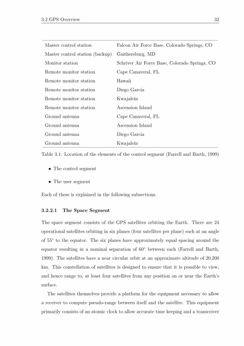
3.2 GPS Overview 32
Master control station Falcon Air Force Base, Colorado Springs, CO
Master control station (backup) Gaithersburg, MD
Monitor station Schriver Air Force Base, Colorado Springs, CO
Remote monitor station Cape Canaveral, FL
Remote monitor station Hawaii
Remote monitor station Diego Garcia
Remote monitor station Kwajalein
Remote monitor station Ascension Island
Ground antenna Cape Canaveral, FL
Ground antenna Ascension Island
Ground antenna Diego Garcia
Ground antenna Kwajalein
Table 3.1: Location of the elements of the control segment (Farrell and Barth, 1999)
• The control segment
• The user segment
Each of these is explained in the following subsections.
3.2.2.1 The Space Segment
The space segment consists of the GPS satellites orbiting the Earth. There are 24
operational satellites orbiting in six planes (four satellites per plane) each at an angle
of 55 to the equator. The six planes have approximately equal spacing around the
equator resulting in a nominal separation of 60 between each (Farrell and Barth,
1999). The satellites have a near circular orbit at an approximate altitude of 20,200
km. This constellation of satellites is designed to ensure that it is possible to view,
and hence range to, at least four satellites from any position on or near the Earth’s
surface.
The satellites themselves provide a platform for the equipment necessary to allow
a receiver to compute pseudo-range between itself and the satellite. This equipment
primarily consists of an atomic clock to allow accurate time keeping and a transceiver

3.2 GPS Overview 33
to receive data from the control segment, and transmit signals to the user segment.
The signals transmitted to the user segment are received on two separate carrier
waves: L1 and L2. These are modulated with timing codes known as C/A and P
and it is these timing codes which are explicitly used to calculate pseudo-ranges.
Superimposed on the timing codes is the navigation message. This message contains
ephemeris data for the satellite from which it is transmitted, and satellite clock error
polynomials which describe the behaviour of the satellite clock with respect to GPS
system time.
3.2.2.2 The Control Segment
The control segment comprises a Master Control Station (MCS), six monitor stations
and four ground antennas. The location of the various elements of the control segment
is represented in table 3.1. The purpose of the control segment is to monitor the health
and status of the space segment. To do this the monitor stations monitor the signals
transmitted by the satellites and relay them to the MCS. The MCS then calculates
the satellite orbit parameters and clock corrections. This data is passed to the ground
antennas for upload to the satellites. The satellites then transmit this data in the
navigation message to the user segment, along with ranging signals.
3.2.2.3 The User Segment
The user segment of the GPS is made up of all the antennas and receivers currently
used to receive and decode the GPS signals from the space segment. These signals
can then be used within the receiver processor to calculate user position and velocity.
This process is described in detail in §3.5. Because a GPS receiver is a simplex device,
the GPS space segment is able to serve an infinite number of user segment receivers.
A further point to add at this stage is that there exist a plethora of different GPS
receivers in what is now a very mature consumer market. These can be generally
categorized into two distinct groups, however: low cost and geodetic. Low cost
receivers are cheap, small, readily available and have recently begun to offer access to
the raw GPS observables; this fuels their increasing use in more precise applications.
Geodetic grade receivers have traditionally provided the highest quality observables

3.3 GPS Observables 34
Figure 3.1: Comparison of received satellite signal and receiver generated signal
to the survey industry and are priced accordingly. They offer access to all the raw
GPS observables, often at various data rates, which can go as high as 100Hz. As a
quick comparison low cost receivers cost approximately £200, and geodetic receivers
can be in the order of £10,000.
3.3 GPS Observables
The GPS satellites are continuously transmitting an RF signal that can be utilised
by a user receiver to determine position and velocity estimates. The receiver uses the
signal from each satellite to calculate the range between it and the satellite along a
direct line of sight at discrete time intervals. These ranges are the GPS observables
and are based on measured time or phase differences between the code received from
the satellite, and one generated within the receiver.
3.3.1 The Code Pseudo-range Observable
In practical terms the pseudo-range measurement is calculated within the receiver
by comparing the receiver generated code with that received from the transmitting
satellite. The principle is that receiver code is generated at the same time as the
satellite code is transmitted and by comparing the two and calculating the time offset
between them, as represented in figure 3.1, it is possible to determine the transit time
of the signal from satellite to receiver. This transit time can then be scaled by the
velocity of light in vacuo to give the line of sight range between receiver and satellite.

3.3 GPS Observables 35
This process is complicated by the fact that different time frames are in use within
the GPS. Satellites are each installed with a precise atomic clock which operates in a
satellite time frame (t). The time of transmission of all signals transmitted from the
satellites is given with reference to this time frame. Receivers also contain there own
quartz clock although this is significantly less accurate than the atomic clocks fitted
to the satellites. The reception times of each signal are recorded with reference to the
receiver clocks in the receiver time frame (τ). Both these time frames are related to
the GPS system time (T ) by:
T = t+ δt (3.1)
T = τ + δτ (3.2)
where δt denotes the satellite clock offset and δτ denotes the receiver clock offset.
There follows a derivation of the pseudo-range observation equation which follows
the notation and convention of Bingley (1998). For the purposes of this derivation a
superscript will denote a satellite related term and a subscript will denote a receiver
related term. It is necessary to define two terms related to the ranging from receiver
to satellite: namely pseudo-range and geometric range.
• Pseudo-range (PR) can be defined as the difference between the time of signal
reception in the receiver time frame (τr) and the time of signal transmission in
the satellite time frame (ts) scaled by the speed of light in vacuo (c).
• Geometric range (ρ) is defined as the difference between the time of signal
reception in the GPS time frame (Tr) and the time of signal transmission in the
GPS time frame (T s) scaled by the speed of light in vacuo.
These definitions lead to the equations:
PRsr = c(τr − ts) (3.3)
ρsr = c(Tr − T s) (3.4)

3.3 GPS Observables 36
substituting equations 3.1 and 3.2 into equation 3.4 yields:
ρsr = c((τr + δτr)− (ts + δts)) (3.5)
rearranging gives:
ρsr = c(τr − ts)− c(δτr − δts) (3.6)
now substituting equation 3.3 into equation 3.6 and rearranging results in the basic
pseudo-range equation.
PRsr = ρs
r − c[δτr − δts] (3.7)
This basic pseudo-range equation needs a more rigorous definition of the time frames
involved before it can be considered complete. Each of the terms in equation 3.7 can
be associated with its time frame thus:
• PRsr is the pseudo-range measured at the receiver in the receiver time frame, ie
PRsr(τr).
• ρsr is the geometric range calculated using the GPS time of reception at the
receiver and the GPS time of transmission from the satellite, ie ρsr(T
s, Tr).
• δτr is the receiver clock offset in the receiver time frame, ie δτr(τr).
• δts is the satellite clock offset measured in the satellite time frame, ie δts(ts).
If these more explicitly defined terms are substituted into equation 3.7 then a more
rigorous pseudo-range equation results. More terms can be added to this equation
to account for common error sources. It is sufficient here to generalise these into
three terms: ionospheric delay (I), tropospheric delay (T ) and miscellaneous errors
(ε). These errors and the methods of compensation for them are discussed in detail
in §3.4.
PRsr(τr) = ρs
r(Ts, Tr)− c[δτr(τr)− δts(ts)] + I + T + ε (3.8)

3.3 GPS Observables 37
3.3.2 The Carrier Phase Pseudo-range Observable
The code signal is modulated onto a carrier signal within the satellite using binary
bi-phase modulation. It is this modulated carrier signal that is transmitted form the
transceiver mounted on the satellite. By measuring the phase of the carrier signal an
observable that can be considered much more precise than that of the code pseudo-
range is be produced. The carrier phase pseudo-range measurement is the difference
between the phase of the carrier signal generated within the receiver, and that which
is received from the satellite. This pseudo-range consists of a fractional carrier phase
element (φsr(τr)) and an integer number of cycles termed the integer ambiguity (N s
r ).
The integer ambiguity is so called because the number of integer cycles is ambiguous
and cannot be determined from the carrier phase pseudo-range measurement.
This new pseudo-range measurement can be substituted into the basic pseudo-
range equation shown in equation 3.7 yielding:
φsr(τr) =
f
cρs
r(Ts, Tr)− f [δτr(τr)− δts(ts)] +N s
r (3.9)
Equation 3.9 shows the basic carrier phase pseudo-range equation. In reality the
receiver will actually make an arbitrary guess at the value of the integer ambiguity
when it first locks on to each satellite. Thus N sr represents the correction required to
that arbitrary guess in order that it represents the true integer ambiguity. Adding in
the error terms introduced in equation 3.8 yields the full carrier phase pseudo-range
equation:
φsr(τr) =
f
cρs
r(Ts, Tr)− f [δτr(τr)− δts(ts)] +N s
r + I + T + ε (3.10)
3.3.3 The Pseudo-range Rate Observable
The Doppler is a measure of the frequency shift of the carrier signal and is measured
routinely within the GPS receiver as an output from the carrier tracking loop (Parkin-
son and Spilker, 1996a). The doppler shift of the signal from the nominal L1 or L2
frequency is caused by a number of factors including motion of the satellite, motion of
the user receiver and errors due to the drift of satellite and receiver clocks. Ignoring

3.3 GPS Observables 38
the error terms and time frames and scaling any frequency shift by the transmitted
frequency over the speed of light in vacuo yields the doppler equation.
Dsr = −
(vs − vr
c· es
r
)L (3.11)
where esr is the line of sight unit vector and L is the nominal transmitted frequency.
The measured Doppler can then be expressed as a pseudo-range rate by incorpo-
rating the receiver clock drift term:
˙PRsr = (vs − vr) ·
rs − rr
|rs − rr|+ ˙δτr + ε (3.12)
3.3.4 Quality of Recorded Observables
Consideration of a generalized receiver architecture concerning the measurement of
the various observables of the GPS can give some indication of their accuracy and
reliability. Generally the measurement of the code pseudo-range observable utilizes a
delay lock loop (DLL) and measurement of carrier phase based observables utilizes a
phase lock loop (PLL) although carrier phase tracking can also be undertaken using
a frequency lock loop. There follows a broad description of the measurement of the
GPS observables using feedback control loops as it relates to the work presented in
this thesis. For a more thorough analysis read van Dierendonck (1996) or Misra and
Enge (2004) although much of the details of receiver architecture are proprietary and
specific to particular manufacturers.
3.3.4.1 Signal Tracking with Feedback Control Loops
After signal acquisition GPS receivers utilise a DLL to track the code signal from each
satellite and a PLL to track the carrier signal. Both DLLs and PLLs are feedback
control loops that use an error signal which is fed back in order to control a process.
In the case of a DLL the error signal is the time difference between the code signal
received from a satellite and the replica code generated within the receiver. Figure 3.2
shows a simplified block schematic representation of a delay lock loop. In figure 3.2

3.3 GPS Observables 39
Figure 3.2: Block schematic representation of a delay lock loop
the DLL is used as a loop filter producing a clean signal output from a noisy signal
input, but the operation of this loop filter adequately demonstrates the principle of a
DLL. The noisy received code signal from the satellite (Sigs + ε) is compared to the
code generated within the receiver (Sigr) to produce a signal proportional to the time
difference between the two (∆t) which is a measure of signal transit time and hence
pseudo-range. Based on this difference signal the control element of the loop issues
commands to the code generator or, more precisely, the code generator clock to slew
the generated code to match the received code.
The operation of a PLL is broadly the same as that of a DLL except that the error
signal in this instance is the difference in phase between the received carrier signal and
the replica carrier generated within the receiver, and that the process to be controlled
is the numerically controlled oscillator within the PLL that governs the phase of the
replica carrier. Here, the error signal gives a measure of carrier phase, although this
measurement is ambiguous in range terms because only the fractional part of a cycle
is recorded and the integer number of complete cycles is unknown.
3.3.4.2 Feedback Control Loop Performance
Analysis of feedback control loop performance falls into two categories: noise perfor-
mance and dynamic performance (Kaplan, 1996; Misra and Enge, 2004). These two
performance characteristics are in direct conflict within a feedback control loop in
that better noise performance will lead to a more sluggish dynamic performance and
vice-versa. This results in a trade off between the two which can be tuned to receiver
requirements.
The tuning of this trade off will have a direct impact on the quality and integrity of
the recorded GPS observables within a given receiver. For example, a receiver designed

3.3 GPS Observables 40
to undergo high dynamics would need feedback control loops with strong dynamic
performance, which may impact on the their noise performance. The opposite could
be true of a receiver designed predominantly for static use.
Errors in the measurement of the GPS observables that occur due to the receiver
itself can be broadly split into to sections: system noise and tracking loop noise.
System noise is made up of the noise introduced by the antenna, the cables and the
electronic componentry within the receiver. Formulae exist with which to accurately
quantify this noise for a given receiver (Langley, 1997) but this is a difficult task in
reality as the parameters required for the calculations are not easy to ascertain. As
a generalisation for the purposes of this thesis the system noise created by a low cost
receiver such as the U-Blox Antaris can be said to be greater than that created by
better grade receivers such as the Novatel OEM4 or Leica 530. System noise has
a great effect on the measurement of the code phase pseudo-range observable, but
little effect on the accuracy of the measurement of the carrier phase pseudo-range
observable although it does affect the dynamic range of the carrier tracking loops
(Kunysz, 1998).
Tracking loop noise is dependent on two factors: tracking loop bandwidth and
signal-to-noise ratio of the GPS signal. This is demonstrated by the approximation
of the formulae for the calculation of the noise contributed by the delay lock loop and
phase lock loop taken from Langley (1997).
σDLL =
√αBL
c/n0
λc (3.13)
σPLL =
√BL
c/n0
λc (3.14)
It is clear that the error in both these loops is very similar. The σDLL and σPLL are
measured in metres, BL is the loop noise bandwidth in Hz, c/n0 is the carrier-to-noise
density (signal-to-noise ratio) of the signal expressed as a ratio (=10C/N0
10 ), λc is the
carrier wave length and α is the delay lock loop discriminator factor. As a guide to
carrier loop noise values σPLL is 0.6 mm when C/N0 is 45 dB-Hz and carrier tracking
loop bandwidth is 15 Hz (values not unexpected in typical GPS receivers).
In summary it can be said that system noise can have a direct impact on the

3.4 GPS Error Sources 41
quality of the code phase pseudo-range observation but not on the quality of the
carrier phase pseudo-range observation, although it can affect the dynamic range of
the carrier tracking loop. Noise introduced by the carrier tracking loop is small and
will not impact heavily on the quality of the carrier phase pseudo-range observable,
but the quality of the componentry used in the loop, such as the numerically controlled
oscillator, can have a significant influence on the carrier tracking loop output (van
Dierendonck, 1996).
In the case of the low cost receiver the carrier phase observation would be expected
to be of a slightly degraded quality compared to that recorded using a higher grade
receiver, perhaps with an increased noise level due to lower grade componments. The
effect of increased system noise on the dynamic range of the carrier tracking loop will
result in a carrier phase pseudo-range observable with a greater number of cycle slips
due to signal loss and could result in greater noise levels due to the need to increase
tracking loop bandwidth.
3.4 GPS Error Sources
GPS measurements recorded by the receiver are corrupted by a number of various
error sources. In most cases techniques are available that can help to mitigate these
errors and so improve the integrity and accuracy of the recorded observables. In this
section the main error sources are discussed along with any mitigation techniques
available.
As part of the GPS heave algorithm developed during this thesis and presented
in chapter 6 both stand-alone user position and velocity are estimated. Stand-alone
position requires that code pseudo-ranges are corrected for absolute errors whereas
the velocity estimation uses temporally differenced carrier phase pseudo-ranges and
so the rate of change of each error source is required. As part of the discussion of
each error source in this section there is also an assessment of the rate of change of
that error source and the likely impact of it upon user velocity estimation.

3.4 GPS Error Sources 42
3.4.1 Satellite Errors
Errors emanating from the satellites fall into two main categories, namely satellite
clock offset and ephemeris error. These both add bias terms into the measurement of
the GPS observables when used to correct the code pseudo-range observable and, in
the case of satellite clock error, can also have a significant effect on velocity estimation
if unmitigated.
3.4.1.1 Satellite Clock Offset
The timing on board the satellites of the GPS is provided by highly accurate atomic
clocks. These clocks are very stable but there will inevitably be some deviation from
GPS time which can be as large as 1 ms (Parkinson and Spilker, 1996a). The deviation
of each satellite’s clock from GPS time is monitored by the control segment, which
then calculates up to three polynomial terms relating to clock bias, clock drift and
clock drift rate. These data are then uploaded to the satellites for broadcast in the
navigation message. They can then be used by the stand-alone positioning user to
correct for the satellite clock offset. The two polynomial terms relating to satellite
clock drift and clock drift rate explicitly describe the rate of change of the satellite
clock error with time.
The polynomials are only an estimation of how the satellite clock offset will prop-
agate into the future and so some of this error will remain for the stand-alone user.
In reality though the residual error will be small enough to be considered negligible,
particularly when considering the rate of change of that residual error. Differential or
interferometric positioning users will be able to completely remove this error as it is
common mode for all receivers.
3.4.1.2 Ephemeris Error
The control segment of the GPS also computes the predicted orbit path of each of
the satellites. The various elements that describe this orbit path are uploaded to
the satellites and, as with the clock polynomials, are transmitted in the navigation
message to form the broadcast ephemeris. The position of each satellite can be

3.4 GPS Error Sources 43
calculated as a function of time based on the broadcast ephemeris although some
residual error will remain due to divergence of the predicted orbit from the actual
orbit over time. This residual error is in the order of 4.2m (1σ) (USDOD, 1991).
Generally, real time users calculate satellite position as a function of time based
on the broadcast ephemeris although precise ephemerides are offered by organizations
such as the International GPS Service. The more accurate of these are available
only with a number of hours latency. As mentioned in §3.5.2, when differential or
interferometric techniques are employed the ephemeris error is largely removed for
short baselines.
When considering the GPS heave algorithm developed for this project satellite ve-
locity, achieved through the use of a central difference algorithm on satellite positions
at adjacent epochs, is required. This parameter is computed in real time based on
the satellite positions calculated using the broadcast ephemeris data in the navigation
message. The velocities derived in this way are accurate to ± 1 mm/s when compared
to the International GPS Service SP3 precise ephemeris velocities (Zhang et al., 2006).
3.4.2 Measurement Errors
Receivers introduce errors and noise as part of the process of measuring the GPS
observables. This can be caused by the algorithms used within the firmware of the
receiver, or can be a function of the quality of componentry used: the low cost receivers
having a greater amount of error. Within the scope of this work receiver error is
particularly important as low cost receivers are used and this can directly impact on
the quality of the measured observables.
3.4.2.1 Receiver Clock Offset
The timing of operations within a GPS receiver is governed by a quartz clock, which is
significantly less stable than the atomic clocks used on board the satellites. The quartz
clock in the receiver introduces a large bias to the measurement of the GPS observables
by the receiver. The stand-alone positioning user has to take a measurement to a
fourth satellite in order to solve for receiver clock error. However, interferometric

3.4 GPS Error Sources 44
positioning users that have calculated the double differenced phase observable have
completely removed the effects of receiver clock.
The rate of change of the receiver clock offset will depend largely on the quality of
the receiver used to collect the raw observables. When processing GPS observables
to estimate user position the receiver clock can also be resolved as part of the least
squares calculation as has been done in the past or it can be differenced away through
the production of the temporal double difference observable developed for this project.
This technique is detailed in chapter 6.
3.4.2.2 Multipath Error
Multipath is the term given to an error source that is caused by the signal from the
GPS satellite taking one or more indirect routes to the receiver. Signals, as well as
taking the direct route to the receiver, can also bounce of objects or buildings that
may be nearby to the receiver antenna, resulting in a pseudo-range measurement that
appears greater than it should. There are techniques available to mitigate the effects
of multipath based on propagation geometry or sidereal analysis but these are not
generally used for navigation purposes and have not been employed on this project.
3.4.2.3 Receiver Noise and Tracking Loop Errors
Measurement errors are also introduced by the receiver tracking loops. These can
take the form of noise or a bias. The noise produced by the receiver is predominantly
thermal noise and is proportional to the quality of the components used. Bias terms
can be introduced by dynamic stress in the tracking loops with the effects often varying
dependent on the algorithms employed in receiver firmware. These bias terms have
particular relevance to the algorithms developed during this project and are analysed
in greater detail in §3.3.4
3.4.3 Propagation Errors
As the GPS signals travel through the earth’s atmosphere they are subject to re-
fraction, which causes a delay in the transit time of the signal. Two regions of the

3.4 GPS Error Sources 45
atmosphere have an effect on the propagation of the radio frequency waves: the
ionosphere and the troposphere. These effects and their mitigation techniques are
discussed below.
3.4.3.1 Ionospheric Effects
The ionosphere occupies a region between 70 km and 1000 km above the earth’s
surface. It is a dispersive medium, which means that the propagation velocity of
radio signals through the medium varies with frequency. The phase pseudo-range
observable and the code pseudo-range observable experience different effects as they
pass through the ionosphere, caused by the different indices of refraction for each.
Generally it can be said that the phase observable will experience an advance, and
the code observable a delay (Misra and Enge, 2004).
The magnitude of the ionospheric effect on the GPS signal is proportional to the
total electron count (TEC) along the signal path. The TEC is a function of time of day,
user location, satellite elevation angle, season, ionizing flux, magnetic activity, sunspot
cycle and scintillation (Kaplan, 1996).There exist models that attempt to compensate
for the effects of the ionosphere, the most commonly used being the Klobuchar model
(Klobuchar, 1996), which is a function of time and latitude. The co-efficients required
in the Klobuchar model are transmitted as part of the navigation message and appear
in the header of the RINEX navigation file. Stand-alone GPS users can make use of
these co-efficients to mitigate range errors caused by the ionosphere but residual errors
will remain due to the inadequacies of the model. The Klobuchar model accounts for
approximately 50% of the effects of the ionosphere at mid latitudes (Farrell and Barth,
1999).
Dual frequency GPS users can take advantage of the dispersive nature of the iono-
sphere to almost completely remove its effects from their observations. Taking pseudo-
range measurements on both the L1 and L2 frequencies transmitted by the GPS allows
the following equation to be employed to estimate the ionospheric correction to the
pseudo-range measured on L1.

3.4 GPS Error Sources 46
IL1 =
(L2
2
L22 − L2
1
)(ρL1 − ρL2) (3.15)
Where L1 and L2 are the frequencies of those signals, and ρL1 and ρL2 are the
pseudo-range measurements recorded on each frequency.
As previously mentioned the ionospheric delay will change as a result of many
factors, the most significant being the elevation angle. As a result models such as
Klobuchar have an elevation dependent mapping function that will alter the computed
delay. The rate of change of the ionospheric delay on the GPS signals will differ
between satellites but empirical data collected during this project suggest velocity
errors in the order of ±1-2 mm/s.
In this thesis the Klobuchar model has been used when observations have been
recorded using a low cost single frequency receiver, and dual frequency removal of the
ionosphere has been used where possible.
3.4.3.2 Tropospheric Delay
The troposphere is the region of the earth’s atmosphere between the surface of the
earth and an altitude of 17 km. The troposphere is a non-dispersive medium so the
delay experienced by signals on both L1 and L2 is the same, and the delay to code
pseudo-ranges is the same as that to phase pseudo-ranges. The troposphere consists
of a wet component and a dry component. Around 90% of the tropospheric delay is
caused by the dry component and can be well modelled (Hoffmann-Wellenhoff et al.,
2001). Under ideal circumstances atmospheric readings such as temperature, pressure
and humidity would be recorded and input into any model but in practice these are
often difficult to obtain and a standard atmosphere model is used instead. The delay
due to the wet component is primarily caused by water vapour and the nature of the
temporal and spatial variations makes this difficult to model.
Tropospheric errors when computing user velocity are similar in nature to those
seen from the ionosphere in so much as they change with elevation. The rate of change
of the error will be predominantly decided by the mapping function of the model used
and satellite elevation. Data collected during the course of this project suggests that
velocity errors up to ±5 mm/s may be seen if the troposphere is unmitigated.

3.5 Obtaining User Position from GPS Observables 47
The non-dispersive nature of the troposphere forces the use of a model for the
stand-alone GPS user to compensate for tropospheric delay. Most simple models
are accurate to about 1 m or better (Parkinson and Spilker, 1996a). The model
employed in this thesis is STANAG (1990). Where differential or interferometric
techniques are employed most of the tropospheric delay can be removed from pseudo-
range observations.
3.5 Obtaining User Position from GPS Observ-
ables
The GPS observables discussed in §3.3 can be utilised in a number of algorithms
to provide the user with instantaneous position and velocity of varying degrees of
accuracy. The simplest of these algorithms is to use the pseudo-range equation to
derive three dimensional position using a single GPS receiver. Other techniques
employ two receivers in order that some of the significant error sources associated with
the GPS can be reduced, and so that use can be made of the more accurate carrier
phase observable. For the purposes of the thesis the following industry accepted
definitions will apply.
• Stand-alone GPS: The use of a single receiver to provide instantaneous user
position.
• Differential GPS: The use of two receivers, one in a fixed known position used
to provide code pseudo-range corrections to the second roving receiver.
• Interferometric GPS: Positioning using two receivers, one in a fixed known
position which provides its carrier phase observations to the second roving
receiver. The roving receiver then uses differencing techniques to calculate a
new, more accurate, observable.
The following subsections present a more detailed description of these techniques.

3.5 Obtaining User Position from GPS Observables 48
3.5.1 Stand-alone GPS
Stand-alone positioning uses the code pseudo-ranges recorded with one gps receiver
to calculate user position. The pseudo-range rate observable from a single receiver
can also be used to calculate user velocity. This type of GPS processing can pro-
duce user position with an accuracy of approximately ten metres and, as such, is
usually considered to inaccurate to be used for marine survey, particularly for vertical
reference.
Three dimensional instantaneous user position is derived from the pseudo-range
observation equation given in equation 3.8. Neglecting the noise term, there are
five unknowns in this equation: geometric range, receiver clock offset, satellite clock
offset, ionospheric delay and tropospheric delay. Atmospheric delays are modelled
during processing and the satellite clock offset is compensated for using navigation
message transmitted from the satellite. There follows a derivation of the linearized
geometric range and a demonstration of its use to solve for user position taken from
Hoffmann-Wellenhoff et al. (2001).
User earth frame position is implicit within the geometric range:
ρsr(T
s, Tr) =√
(Xs −Xr)2 + (Y s − Yr)2 + (Zs − Zr)2 (3.16)
where Xs, Ys and Zs are the earth frame co-ordinates of the satellite and Xr, Yr and
Zr are the earth frame co-ordinates of the receiver. The satellite positions are
calculated from the ephemeris data leaving four unknowns to be solved, and
requiring pseudo-range measurements from at least four satellites.
Once all the terms that can be modelled or compensated for have been removed
the pseudo-range observation equation becomes
PRsr = ρs
r + cδτr (3.17)
This equation is non-linear and so must be linearized about an initial position es-
timate. This enables the system of equations that the pseudo-range measurements
produce to be solved using a least squares process. Linearization begins by defining
an estimated geometric range from the initial position estimate:

3.5 Obtaining User Position from GPS Observables 49
ρsr0 =
√(Xs −Xr0)2 + (Y s − Yr0)2 + (Zs − Zr0)2 (3.18)
≡ f(Xr0, Yr0, Zr0) (3.19)
Where Xr0, Yr0 and Zr0 are the earth frame co-ordinates of the initial position
estimate. Equation 3.16 can also be written as f(Xr, Yr, Zr).
The unknown user position values can be written as
Xr = Xr0 + ∆Xr (3.20)
Yr = Yr0 + ∆Yr (3.21)
Zr = Zr0 + ∆Zr (3.22)
This introduces the new unknowns of ∆Xr, ∆Yr and ∆Zr, which are the required
corrections to the initial position estimate. These new representations of user
position allow the replacement of f(Xr, Yr, Zr) with the equivalent function
f(Xr0 + ∆Xr, Yr0 + ∆Yr, Zr0 + ∆Zr). Using a first order, and hence linear, Taylor
series expansion with respect to the initial position estimate yields
f(Xr, Yr, Zr) ≡ f(Xr0 + ∆Xr, Yr0 + ∆Yr, Zr0 + ∆Zr) (3.23)
= f(Xr0, Yr0, Zr0) +∂f(Xr0, Yr0, Zr0)
∂Xr0
∆Xr (3.24)
+∂f(Xr0, Yr0, Zr0)
∂Yr0
∆Yr +∂f(Xr0, Yr0, Zr0)
∂Zr0
∆Zr
The partial derivatives of equation 3.24 can be calculated as
∂f(Xr0, Yr0, Zr0)
∂Xr0
= −Xs −Xr0
ρsr0
(3.25)
∂f(Xr0, Yr0, Zr0)
∂Yr0
= −Ys − Yr0
ρsr0
(3.26)
∂f(Xr0, Yr0, Zr0)
∂Zr0
= −Zs − Zr0
ρsr0
(3.27)

3.5 Obtaining User Position from GPS Observables 50
which, along with equation 3.19, can be substituted into equation 3.24 to yield the
geometric range equation linearized with respect to ∆Xr, ∆Yr and ∆Zr:
ρsr = ρs
r0 −Xs −Xr0
ρsr0
∆Xr −Y s − Yr0
ρsr0
∆Yr (3.28)
−Zs − Zr0
ρsr0
∆Zr
The linearized geometric range can then be substituted into the pseudo-range equation
derived in §3.3, which can subsequently be used to create a system of equations
solvable using a least squares. An example of this is given below that neglects
atmospheric terms which can be modelled or mitigated as explained in §3.4, and
assumes the satellite clock bias is known from the navigation message.
PRsr = ρs
r0 −Xs −Xr0
ρsr0
∆Xr −Y s − Yr0
ρsr0
∆Yr (3.29)
−Zs − Zr0
ρsr0
∆Zr − c[δts − δτr]
Collecting the known terms on the left side of the equation yields
PRsr − ρs
r0 − δts = −Xs −Xr0
ρsr0
∆Xr −Y s − Yr0
ρsr0
∆Yr (3.30)
−Zs − Zr0
ρsr0
∆Zr + cδτr
This equation clearly has four unknown terms: ∆Xr, ∆Yr, ∆Zr and δτr, requiring four
equations, or pseudo-range measurements from separate satellites, in order to solve
for all of them. In order to simplify these sets of equations the following shorthand
representations will be used.
ls = PRsr − ρs
r0 + δts
asXr
= −Xs −Xr0
ρsr0
asYr
= −Ys − Yr0
ρsr0
asZr
= −Zs − Zr0
ρsr0

3.5 Obtaining User Position from GPS Observables 51
These allow the much simplified expression of the series of equations required to solve
for instantaneous user position; the satellites are numbered s1 to s4:
ls1 = as1Xr
∆Xr + as1Yr
∆Yr + as1Zr
∆Zr + cδτ (3.31)
ls2 = as2Xr
∆Xr + as2Yr
∆Yr + as2Zr
∆Zr + cδτ
ls3 = as3Xr
∆Xr + as3Yr
∆Yr + as3Zr
∆Zr + cδτ
ls4 = as4Xr
∆Xr + as4Yr
∆Yr + as4Zr
∆Zr + cδτ
The set of equations in 3.31 can be presented in matrix form by
l = A x (3.32)
where
l =
ls1
ls2
ls3
ls4
(3.33)
A =
as1Xr
as1Yr
as1Zr
c
as2Xr
as2Yr
as2Zr
c
as3Xr
as3Yr
as3Zr
c
as4Xr
as4Yr
as4Zr
c
(3.34)
x =
∆Xr
∆Xr
∆Xr
δτ
(3.35)
Solving for x allows the estimation of the required corrections to the initial position
estimate, and also the receiver clock offset.

3.5 Obtaining User Position from GPS Observables 52
3.5.2 Differential Positioning
Differential GPS (DGPS) positioning is a technique that allows for the mitigation of
many of the errors associated with stand-alone GPS. The technique utilizes two GPS
receivers, with one reference receiver commonly placed over a fixed and known point.
The basic principle is that the known position of the reference receiver can be used
to calculate a correction to each measured pseudo-range that accounts for the errors
introduced by both the control and space segments of the GPS. The pseudo-range
corrections can then be transmitted in real time to other receivers in the vicinity
of the reference receiver and used to compensate for the same errors in their own
pseudo-range measurements.
The mitigation of errors associated with stand-alone GPS can improve the position
accuracy obtainable to less than five metres. DGPS is routinely used in hydrographic
survey to provide plan position of the survey vessel, It is, however, still considered
too inaccurate to provide any vertical reference and the setup for the majority of
hydrographic survey vessels is to use DGPS to calculate horizontal position and then
use an inertial based heave motion sensor to give vertical reference.
A generalization of the basic pseudo-range equation for a receiver, A, highlights
the range biases caused by each of the GPS segments:
PRsA = ρs
A + ∆ρsA + ∆ρs + ∆ρA (3.36)
The ∆ρsA term represents the errors caused by the control segment and receiver
position such as ephemeris error and atmospheric effects, ∆ρs are those errors which
are due solely to the satellite such as satellite clock offset and ∆ρA are receiver
dependent errors such as receiver clock offset and multipath. From equation 3.36
it is possible to derive a pseudo-range correction term:
PRCs = ρsA − PRs
A (3.37)
This can be calculated for the reference receiver because the receiver position is known,
allowing the calculation of ρsA. Now the pseudo-range measurement to the same
satellite but from a second receiver, B, can be corrected for the majority of the errors:

3.5 Obtaining User Position from GPS Observables 53
PRsB = ρs
B + ∆ρsB + ∆ρs + ∆ρB (3.38)
PRsBCorr = PRs
B + PRCs (3.39)
PRsBCorr = ρs
B + [∆ρsB −∆ρs
A] + [∆ρs −∆ρs] + [∆ρB −∆ρA] (3.40)
The satellite dependent terms cancel completely and, provided the distance between
the roving receiver and the reference receiver is not too great, so do the orbit and
atmospheric errors. Removing the satellite related terms and neglecting the satellite
to receiver errors yields
PRsBCorr = ρs
B + ∆ρBA (3.41)
where, if multipath is neglected, the term ∆ρBA is the difference between the receiver
clock bias of the two receivers. A system of corrected pseudo-range equations can
then be formed and solved for in exactly the same way as shown in §3.5.1.
3.5.3 Interferometric Positioning
Interferometric positioning, as with differential positioning, uses two receivers, one
commonly set up over a fixed known point. However, instead of calculating a cor-
rection term, carrier phase observations from different receivers and satellites are
differenced to produce an observable with many of the errors mitigated or removed.
This can be done in real time via a suitable transmission media, or as a post processing
technique.
3.5.3.1 Single Difference
The single differencing is the process of differencing two carrier phase observations
either from the same satellite to different receivers (differencing across receivers) or
from different satellites to the same receiver (differencing across satellites). The
single difference observable is often considered to be that resulting from differencing
across receivers but in either case results in the cancellation of common mode errors.

3.5 Obtaining User Position from GPS Observables 54
The single difference observation equation results from the differencing of the phase
pseudo-range equation 3.10 to satellite, E, from two receivers, A and B.
φEAB = φE
B − φEA (3.42)
=f
cρE
AB − fδτAB +NEAB + IE
AB + TEAB (3.43)
The satellite clock offset terms have cancelled out and for moderate distances from the
reference receiver the ephemeris errors and atmospheric effects are greatly reduced.
Single difference observation equations to satellites N, O and V can also be produced.
These can then be processed using on-the-fly ambiguity resolution techniques, or used
as the basis for the formation of the double difference observation equation.
3.5.3.2 Double Difference
The double difference observation equation is now formed by differencing the single
difference equations derived in the previous section. The second difference is a
difference across satellites and so removes the common mode error, in this case the
receiver clock offset. An example of a double difference equation using two receivers,
A and B, and two satellites, E and N is given below.
φENAB = φN
AB − φEAB (3.44)
=f
cρEN
AB +NENAB + IEN
AB + TENAB (3.45)
If two more of these double difference observation equations are formed then they can
be processed using OTF ambiguity resolution techniques to provide highly accurate
positioning.
3.5.4 Spacial Decorrelation
The spacial decorrelation of the ephemeris and atmospheric errors mentioned in the
§3.5.2 and 3.5.3 is shown clearly in figure 3.3. It can be seen that the further away
the roving receiver is from the reference receiver the greater the change in the line

3.6 Obtaining User Velocity from a Stand-alone GPS Receiver 55
Figure 3.3: Spacial decorrelation of DGPS corrections
of sight vector to the satellite. This change in the line of sight vector results in the
signal passing through a different amount of atmosphere and also a different section
of atmosphere. In addition the correction to the range errors associated with the
broadcast ephemeris also only apply along the line of sight vector between satellite
and reference receiver. As the roving receiver moves further away from the reference
receiver the greater the change in the line of sight vector and the less relevant the
correction for both atmospheric and ephemeris errors.
3.6 Obtaining User Velocity from a Stand-alone
GPS Receiver
The GPS provides the user with the ability to calculate three dimensional velocity as
well as position. This can be done in a number of ways, the simplest of which is to
form an approximate derivative of user position. However, the work contained within
this thesis is primarily concerned with stand-alone GPS and under these conditions
user position is not accurate enough to be able to adequately determine user position
in this way. This section concentrates on the two most accurate methods of calculating
user position from a stand-alone GPS receiver.

3.6 Obtaining User Velocity from a Stand-alone GPS Receiver 56
3.6.1 Velocity from the Pseudo-range Rate Observable
Various techniques exist to process the pseudo-range rate observable to obtain user
velocity, one such technique taken from Kaplan (1996) is given below.
The doppler equation taken from 3.11 can be written as
f sr = fTs
[1− 1
c[(vs − vr) · es
r]]
(3.46)
where f sr is the doppler shifted frequency, fTs is the satellite transmitted frequency,
vs and vr are the satellite and receiver velocity and esr is the line of sight unit vector
between satellite and receiver. The transmitted frequency from the satellite is based
on the atomic clock installed on it. The true transmitted frequency will, therefore,
differ from the nominal frequency by an amount proportional to the satellite clock
drift given by the polynomials in the navigation message. Therefore
fTs = f0 + ∆fTs (3.47)
where f0 is the nominal transmitted frequency (either L1 or L2) and ∆fTs is the
correction to the nominal frequency based on the satellite clock error polynomials.
The measured received frequency (f srRx) is also in error by an amount proportional
to receiver clock drift (δτ) and can be related to the doppler shifted frequency
through the relationship
f sr = f s
rRx(1 + δτ) (3.48)
where δτ is positive for a receiver clock running faster than GPS system time.
Equation 3.48 can now be substituted into equation 3.46 to yield
f sr (1 + δτ) = fTs
[1− 1
c[(vs − vr) · es
r]]
(3.49)
which, after moving all known terms to the left, becomes

3.6 Obtaining User Velocity from a Stand-alone GPS Receiver 57
c(f sr − fTs)
fTs+ vs · es
r = vr · esr −
cf sr δτ
fTs(3.50)
The term fsr
fTs on the right hand side of the equation is very close to 1 and this
approximation will result in little error. Collecting the left hand side terms together
and expanding the dot product on the right hand side yields
dsr = vrXe
srX + vrY e
srY + vrZe
srZ − cδτ (3.51)
If at least four such equations are formed using measurements from separate satel-
lites then similarities are obvious between this and the set of equations 3.31. Indeed
this system of equations can be solved for in exactly the same way to yield an estimate
of user position and receiver clock drift.
3.6.2 Velocity from Temporally Differenced Carrier Phase
Observables
Another method of extracting user velocity from a stand-alone GPS receiver is ob-
tained through differencing two temporally adjacent carrier phase pseudo-range ob-
servations (Itani et al., 2000; Serrano et al., 2004a,b; van Graas and Soloviev, 2004).
From this temporal differencing a doppler observable is derived based on the carrier
phase pseudo-range observable. This new carrier based doppler observable is averaged
over a much longer time than the pseudo-range rate observable, which provides almost
instantaneous doppler, and so contains significantly less noise (Serrano et al., 2004a).
This form of velocity estimation from a stand-alone GPS receiver forms the main-
stay of the research presented in this thesis. As such a detailed explanation of the
approach is given in Chapter 6 along with a derivation of all the equations required.
Chapter 4
Vertical Reference for
Hydrographic Survey
4.1 Introduction
Hydrographic survey is the process of recording depth, or bathymetry, data with the
intention of producing a chart that shows the relief of the sea bed being surveyed.
The bathymetry data is usually recorded from a vessel that is on or below the surface
of the sea and most commonly involves echo sounder technology.
Survey vessels on the sea surface undergo vertical displacement due to wave and
tidal effects, resulting in a echo sounder platform that is never truly stationary.
Vertical reference must be provided for the echo sounder transponder firstly so that
the bathymetry data can be reduced to a meaningful datum, and also so that motion
of the vessel due to waves and tides can be compensated for and removed from the
bathymetry data. Failure to do so would result in vessel motion appearing as noise
on the plotted relief of the sea bed as changes to vessel height actually manifest as
changes in recorded depth by the echo sounder.
This chapter looks in detail at the current practices in providing vertical reference
to hydrographic surveys and explains their significance to the hydrographic survey
industry. There is a strong focus on heave measurement and in depth analysis of
the current classical methods of heave measurement used within the industry. The
58

4.2 Chart Datum 59
errors and problems with classical heave measurement highlighted in this chapter are
exactly those which the GPS based heave measurement method developed as part of
this project have overcome.
4.2 Chart Datum
The purpose of hydrographic surveying is to measure the depth of a body of water
with the intention of depicting the relief of the seabed, in a manner similar to the
topographic mapping of land areas (Ingham, 1992). For this data to be of use to
mariners in the form of charts, the depth to the seabed must be given relative to
a common datum. This datum is often referred to as chart datum and, in the
current hydrographic industry, is usually selected to be coincident with the lowest
astronomical tide or mean lowest low water (MLLW) (Milne 1980).
Nautical charts express the relief of the seabed by showing depths relative to chart
datum, as explained by the Admiralty (1987). It is for this reason that chart datum
has traditionally been chosen to be coincident with MLLW as it will always display
the depth of the water when at its most shallow, which has obvious implications for
safety. The main problem with the use of MLLW as the chart datum is that this level
is locally affected and consequently not consistent along a given stretch of coastline.
Because tides are locally specific they change from area to area, which can produce
vastly different tidal regimes over relatively short distances, and even across the face
of a single chart.
A true definition of chart datum is the height reference surface used in hydrography
(Martin and Broadbent, 2004), and is currently accepted to be MLLW. Moves are
underway, however to standardize chart datum to an ellipsoidal reference, and the
time is approaching when charted depths may be given to a geodetic, rather than
local, datum.

4.3 Classical Hydrographic Methods 60
Figure 4.1: Discrete tidal zones surrounding Popof Island, Alaska
4.3 Classical Hydrographic Methods
The classical method for the providence of vertical reference to survey vessels takes
the view that vertical vessel motion can be split into the two discrete categories of
tidal motion and heave motion. Tidal motion refers to the low frequency and long
period motion of the vessel due to tidal effects, and heave motion is the relatively
higher frequency shorter period motion experienced by the vessel as a result of waves.
Whilst some more modern and more expensive systems, discussed in §4.4, consider
the motion of the vessel across the entire frequency range, the classical methods are
still widely practiced within the industry. They are often favoured due to their ease
of use and relatively low cost when compared to techniques that use a single water
level correction. This section looks at methods of providing compensation for tidal
and heave motion of a survey vessel.
4.3.1 Tidal Compensation
Tidal effects on the vertical position are seen as low-frequency vertical displacements
of the vessel. They are caused primarily by astronomical effects, but can also be

4.3 Classical Hydrographic Methods 61
Figure 4.2: Sketch detailing the parameters necessary for tidal compensation
influenced by meteorological and oceanographic factors. This vertical displacement
of the survey vessel must be accounted for in any reduction of bathymetric data as
it actually represents an increase or decrease in recorded depth; uncompensated this
would translate into changes in the height of the seabed.
Compensation for tide in hydrographic surveying is complicated by the fact that
surveys are seldom conducted in close proximity to tide gauges. Often the survey
area can be several nautical miles from the gauge itself and, in areas of complex tidal
systems, this can cause significant errors when the calculation of the tide at the survey
site is attempted.
The predominant method for the transference of tidal data to the survey site is
through discrete tidal zoning, a system that defines areas of similar tidal characteris-
tics using polygons, or discrete zones (Imahori et al., 2003). An example of these zones
is seen in figure 4.1, which shows the discrete zone makeup around Popof Island off
the Alaskan coast. This data is a good example of how an area of ocean surrounding
a tide gauge is split into discrete zones. Along with the data describing the shape and
position of the discrete zones comes a time and range offset for each. These offsets
must be applied to the tide data collected at the gauge to produce the tidal effects
experienced in a given zone.
Other techniques exist that allow for the transference of tide reduction data to
a survey site. Chang and Sun (2004) used GPS measurements taken at tide gauge

4.3 Classical Hydrographic Methods 62
sites to reduce the errors associated with transferring data away from the tide gauge.
Also GPS-tracked buoys may be temporarily installed at survey sites, which can then
be used to provide tidal reduction data from the site at which the survey is to be
conducted (Ashkenazi et al., 1996; Chang and Sun, 2004; Bisnath et al., 2004). A
further method is to use interferometric GPS techniques, sometimes in a GPS-aided
INS system, to provide tidal motion of the vessel itself (Sanders, 2003; Zhoa et al.,
2004). This involves the installation of the GPS equipment on board the vessel, long
period vertical displacement can then be used to correct for the motion of the vessel
directly.
Once suitable tide data has been established at the survey site, the process of
compensating for tidal motion is relatively simple. Figure 4.2 shows the parameters
in the process of bathymetry reduction using tide data remote from the survey site.
The result of the tidal compensation is the reduced depth, which can be easily achieved
from
RD = DS − T (4.1)
where RD is Reduced Depth, DS is Depth Sounding and T is Tide level.
4.3.2 Heave Compensation
Equation 4.1 and figure 4.2 offer a simplified model of how bathymetry can be reduced
to chart datum, assuming that the survey vessel is stationary on a perfectly flat
sea surface. This is never the case and real sea conditions contain short period
perturbations from the mean sea level caused by such things as weather, the wake of
other vessels and currents (Alkan, 2003). These perturbations from mean sea level are
termed heave and are perceived by the hydrographer as changes in measured depth,
or noise on the depth soundings and, as such, must be compensated for to improve
the accuracy of the bathymetry.
Heave is a very localized phenomenon, even more so than tide, and so must be
recorded and compensated for on board the survey vessel. There are two main
methodologies for the reduction of heave noise in bathymetry data as discussed by

4.3 Classical Hydrographic Methods 63
Kielland and Hagglund (1995).
4.3.2.1 Analogue Heave Reduction
A method of heave compensation now practically unseen in the industry, analogue
heave reduction is based on the use of analogue data collection during hydrographic
surveys. This equipment collects data and displays a trace of the seafloor representa-
tion to the hydrographer, which can then be used to remove any obvious heave noise
visually. The nature of the analogue data collection precludes any attempt to correct
for heave measurement automatically. There are major shortcomings associated with
this method of heave reduction, particularly if the seafloor is rough, making the
separation of heave and seafloor artefacts more difficult.
4.3.2.2 Digital Heave Compensation
This technique is used in most modern surveys and also forms the backbone of the
majority of research in the field of heave compensation. If survey data is collected
digitally, it becomes possible to measure the vessel heave motion and correct each
sounding as it is recorded.
Within the hydrographic survey industry this is typically done using inertial tech-
nology to measure the vertical acceleration of the vessel, which can be double inte-
grated to produce vertical displacement. The vertical displacement of the vessel can
be used to correct each sounding in real time as it is logged from the echo sounder.
Systems measuring heave in this way are provided by many manufacturers and this
process of heave measurement is discussed in detail in Chapter 5.
Methods of heave compensation that utilise GPS technology are also available.
Much of the research into the use of GPS for vertical reference for hydrographic
survey, however, has been concentrated on its use for single water level corrections
and is discussed in §4.4. There was an early attempt by Kielland and Hagglund
(1995) to use DGPS to measure heave motion of a vessel. This resulted in heave
measurement of the order of ±1 decimetre which underperforms inertial based heave
sensors, which routinely achieve errors at the ±5 centimetre level (VTTSS Ltd, 2005;
Kongsberg, 2005). In addition there is the obvious drawback of the need to have

4.3 Classical Hydrographic Methods 64
multiple receivers for any differential GPS approach. The technique was, however,
shown to have significant cost advantages over inertial based heave sensors.
Approaches to providing GPS based heave using GPS velocities are also known.
There are two papers in particular, the work in which has been built upon by the
work in this thesis. In their paper Itani et al. (2000) developed a wave sensor based
on low cost GPS receivers that monitors wave heights to aid in the collection of
meteorological records, building of breakwaters and tsunami warnings. The work
detailed in the paper is based upon measurements taken with a Furuno GN-77 low
cost GPS receiver. Velocity estimates were calculated using the temporally differenced
carrier phase technique outlined in §3.6 and explained in detail in Chapter 6. The
vertical velocity calculated was then integrated to produce relative vertical position,
any drift in this relative position caused by bias errors in the calculated velocity was
filtered out with a simple high pass filter. Heave outputs were compared to wave
heights calculated using interferometric GPS, and were found to agree to within a ±8
centimetres, a level of performance just below that of inertial based heave sensors.
The work undertaken by Itani et al. (2000) shows the ability of low-cost GPS receivers
to measure heave with a slightly degraded accuracy when compared to inertial based
sensors.
The work of Itani et al. (2000) was endorsed by Reinking and Harting (2002) who
used a Leica 530 geodetic grade receiver to calculate GPS velocities and, subsequently,
heave in a similar way. Comparison in that instance was with both interferometric
GPS and the heave output from a TSS DMS-25 inertial based heave sensor. The heave
output created using temporally differenced carrier phase pseudo-range observations
from the Leica geodetic receivers was found to be of equivalent accuracy to that whaich
can be produced by an inertial based system although in that work the inertial outputs
were post processed forwards and backwards through a high pass filter.
Both these papers demonstrated the ability of an algorithm based on GPS velocities
to measure heave but only Itani et al. (2000) looked at the use of low cost receivers
for heave measurement. The receiver used in that instance was a Furuno G-77 and
carrier phase observations were not available from this unit to the general consumer.
Indeed the U-Blox Antaris receiver used during the work carried out for this project

4.3 Classical Hydrographic Methods 65
is one of the first low cost receivers to offer raw carrier phase observations making
this project the first to look at heave measurement using off the shelf low cost GPS
receivers. Itani et al. (2000) compared a low cost GPS heave output to post processed
float solution GPS heave but does not assess the performance of low cost receivers
against geodetic grade receivers, nor does it compare the results of the algorithm to
either an inertial based sensor or an accurate reference such as the Applanix POS-RS
system held by the IESSG.
It is worth noting that none of the GPS based heave measurement techniques
have been accepted into the hydrographic survey industry to date. The industry is
still dominated by inertial based heave and attitude sensors, primarily because vessel
attitude is often required for steering of the echo sounder beam and this is currently
not available using a GPS only system.
4.3.3 Errors and Problems Associated with Classical Hydro-
graphic Methods
The use of classical methods for vertical reference of hydrographic surveys has asso-
ciated with it some shortcomings that limit the accuracy obtainable. This subsection
will discuss some of those shortcomings.
4.3.3.1 Tide Specific Errors
The methods of tidal reduction involving transference of tide data away from the tide
gauge site to the survey site will obviously introduce some error into the tide data. Any
model chosen to do this will have within it inherent inaccuracies due to unmodelled
parameters. This is largely a result of tidal motion being essentially an unknown
quantity away from coastlines and significant ports. In addition to this there are
further inaccuracies associated with any discretization of an analogue motion. The
attempt to group together areas of similar tidal behaviour into discrete zones can
lead to such quantization errors in the discrete tidal zoning system. The nature of the
algorithm can suggest step changes in sea level at the junction between two zones, a
scenario which is empirically unsound.

4.3 Classical Hydrographic Methods 66
Methods that incorporate GPS techniques also have usability and accuracy prob-
lems associated with them. Installation of GPS-tracked buoys at the survey site is
required for not less than 29 days before the survey is conducted in order that the tide
data conforms to the International Hydrographic Office Standards for Hydrographic
Survey (IHO, 1998). The same document also requires that tide data be expressed in
terms of both chart datum and a suitable geocentric reference system such as WGS84.
This is far easier on shore where the separation between these two datums is much
more clearly defined.
4.3.3.2 Heave Specific Errors
Errors and usability issues in the measurement of heave data differ depending on
the technique employed. Errors associated with an analogue heave compensation
approach are obvious in that they rely on the human eye to pick out heave artefacts
from a trace of the recorded bathymetry. This practice is almost non-existent within
hydrography now but is still worth noting as it demonstrates how far vertical reference
of hydrographic survey has come in a relatively short space of time.
Digital heave compensation can be split into two main categories: the industry
accepted standard of the measurement of heave using inertial sensors; and the mea-
surement of heave using GPS, which has been largely restricted to academic research.
Inertial based systems have a number of common usability issues that make life
more difficult for the hydrographer. They frequently have different filter tuning
settings that must be calibrated to suit the dynamics of the particular vessel they
are fitted to. They can also have a setting that the hydrographer must set manually
for varying sea states. Further to these complications the filter used in a real time
heave algorithm has a certain transient response to large inputs which results in a
‘ringing’ of the output. Large inputs to the heave filter occur during vessel turns
and, as such, the filter must be given time to settle after turns before it is working
optimally. This adds extra length to each survey line and increases the time required
for the survey. When using inertial systems to compensate for heave displacement the
accuracy of the systems is often quoted to be in the order of ±5 centimetres or 5%
of the heave displacement, whichever is the greater (VTTSS Ltd, 2005; Kongsberg,

4.3 Classical Hydrographic Methods 67
Figure 4.3: Bode plot of the frequency ranges represented in the classical method of
providing vertical hydrographic survey reference
2005). This figure relies on the filter being optimally tuned and fully settled. These
errors and problems are discussed in more detail in chapter 5 after the inertial based
heave algorithm developed during this project has been discussed and its performance
has been analysed.
Heave measurement using the stand-alone GPS can overcome many of the issues
that are present with the inertial based systems: they offer a more temporally stable
heave solution, can remove the need for manual input and also potentially provide
savings in cost. There are, however, drawbacks to their use, particularly the fact
that they rely on a good view of the sky and that, if they are to provide equivalent
accuracy to inertial based systems, they are not real time. For most hydrographic
survey requirements, however, enough satellites would be available to provide an
output. As for real time heave compensation of bathymetry, this is unnecessary in a
practical surveying sense and only really serves to give the hydrographer confidence
in the operation of the on board equipment; a near real time output could do this
equally well.
4.3.3.3 General Classical Methodology Errors
The use of the classical methodology to provide vertical reference for hydrographic
survey has, inherent within it, errors associated with the model of sea surface motion it

4.4 Single Water Level Correction 68
uses. It is assumed that all heave motion of the vessel is contained within a particular
frequency band, and that the only other influence on the vertical displacement of
the vessel is tidal. Figure 4.3 shows a bode plot that demonstrates the frequency
of motion that is missed when the classical methodology is implemented. Typically
heave motion is considered to be all vertical vessel motion above approximately 0.03
Hz, while the highest frequency of tidal motion is in the region of 20 µHz (a semi-
diurnal period). Any motion outside of these frequency bands will not be measured
using the classical methodology.
4.4 Single Water Level Correction
Many of the more modern survey reference systems fitted to hydrographic survey ves-
sels now offer a reference based on the WGS84 ellipsoid. They are either GPS based,
or GPS aided, provide an easy way to reduce bathymetry data to a global datum
and compensate for vessel motion across the whole frequency spectrum. This section
deals with the predominant technologies currently employed within the industry and
covers the main areas of research in the field.
4.4.1 GPS-aided INS
For many years GPS and INS sensors have been coupled together in a complete system
to provide accurate position and orientation data at high data rates. This has been
especially useful in the survey industry and is now accepted as the ‘gold standard’
in terms of accurate survey reference data. The technique for coupling the GPS
and INS sensors is well documented and based on the implementation of a Kalman
Filter (Kalman, 1960; Maybeck, 1979; Gelb, 1982; Welch and Bishop, 2001; Hide,
2003). A market leader in the design, manufacture and supply of these equipments to
the hydrographic survey industry is Applanix Corporation. For this reason an brief
overview of the Applanix Position and Orientation System/Marine Vessels (POS/MV)
system follows; the principles of this system can be generally applied to many GPS-
aided INS systems provided by other manufacturers.
The POS/MV is a system produced by Applanix Corporation, a company spe-

4.4 Single Water Level Correction 69
Figure 4.4: Block schematic diacgram of a POS/MV 320
cializing in GPS-aided INS products for the survey industry and based in Toronto,
Canada. The system is designed around the Applanix POS, which is the root of
all Applanix systems, and uses interferometric GPS measurements to aid an inertial
navigation system. It is fitted to hydrographic survey vessels to deliver a highly
accurate position and orientation solution with direct applications for hydrographic
survey. A POS/MV 320 consists of the following components:
• A POS Computer System (PCS)
• A Litton LN200 Inertial Measurement Unit
• A primary GPS Receiver Antenna
• A secondary GPS Receiver Antenna
These components form a loosely coupled system as shown in figure 4.4. The IMU
is the primary sensor, which is aided by the differential GPS measurements obtained
from the primary GPS antenna via an integration Kalman Filter (Mostafa et al., 2001).
The GPS Azimuth Measurement Subsystem (GAMS) uses GPS data from both the
primary and secondary GPS antennas, which are positioned on a fixed baseline, to
produce a heading aiding output. This overcomes the heading drift problems that can
be experienced without GAMS when a vessel holds a particular heading for extended
periods (Hide et al., 2004). The POS/MV 320 has recently been superseded by the

4.4 Single Water Level Correction 70
POS/MV V4 which incorporates a tightly coupled design (Canter and Corcoran,
2004).
The POS/MV can be used to output data in real time, and will also log it for post
processing after completion of the survey. Data is logged in 12MB files onto the PCS
hard drive. Each of these files contains groups in which different types of data are
stored (Corcoran and Pronk, 2003).
4.4.2 Interferometric GPS
As well as providing aiding data to INS sensors, interferometric GPS has also been
used separately to reduce bathymetry data to a suitable datum (Scarfe, 2002; Riley
et al., 2003; Terai, 2004). The principle again involves a single water level correction
as opposed to the classical methodology previously discussed and has the advantage
of being able to describe the vertical motion of the vessel across the entire frequency
range.
4.4.3 Factors Prohibitive to the Widespread Use of Single
Water Level Correction Techniques
The common theme for methods of providing vertical reference using a single water
level correction is that they all involve the use of interferometric GPS. The use of this
equipment brings along with it a set of usability issues that may prohibit its endemic
use in the hydrographic industry. These issues, along with some others, are outlined
in this section.
4.4.3.1 GPS-aided INS Specific Factors
The main factor that prohibits widespread use of GPS-aided INS systems in hydro-
graphic survey is cost. It is widely accepted that these systems provide the best
possible reference data for hydrographic survey, but when this level of accuracy is not
required the cost of the equipment cannot be justified.
Further to this factors discussed in the following subsections will also apply to
GPS-aided INS systems.

4.4 Single Water Level Correction 71
4.4.3.2 Interferometric GPS Specific Factors
As explained in §3.5.3, interferometric GPS involves the use of multiple receivers, one
acting as a reference. Whilst there are now networks of reference stations operated
by various organisations throughout the UK such as the Ordnance Survey, in many
cases the reference station must be provided by the agency undertaking the survey.
This results in the need for two GPS receivers (assuming only one on the vessel), one
being set up over a known point within a moderate distance of the survey site.
Anecdotal evidence suggests that the setting up and running of the reference
receiver is considered by hydrographers to be a ‘fiddly’ and time consuming process
that is prone to error. The truth of this perception can be argued either way but
the fact that it exists suggests that there is a certain inertia within the industry to
the take up of this technology. Added to this there are also limitations to the use
of interferometric GPS offshore due to spatial decorrelation and the expense involved
with the use of multiple geodetic grade receivers.
4.4.3.3 General Single Water Level Correction Methodology Factors
Generally there exists a problem with the use of single water level corrections for
vertical reference of hydrographic survey; this is that they can only provide data
reduced to the WGS84 geodetic reference ellipsoid. The hydrographic survey industry
is currently entrenched in a system that provides charts reduced to chart datum, a
natural system to do when it is considered that the important information on a chart
for navigators and pilots is depth. Consequently, all bathymetry data must currently
be provided reduced to chart datum as well as to the WGS84 ellipsoid (IHO, 1998),
resulting in the need to have a well defined model for the separation of the geoid
and the WGS84 ellipsoid. The day may be approaching when the entire industry
moves over to an ellipsoidal based system but industry inertia may resist this for
some years. Until then there is always the possibility of introducing errors when
modelling ellipsoidal-geoidal separation as the parameter may be clearly defined in
areas of high interest such as major ports, but in many areas of the world it is not.
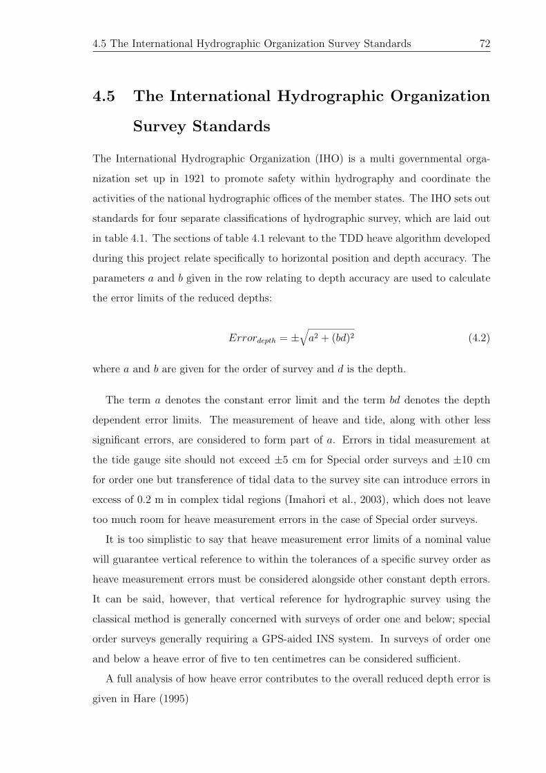
4.5 The International Hydrographic Organization Survey Standards 72
4.5 The International Hydrographic Organization
Survey Standards
The International Hydrographic Organization (IHO) is a multi governmental orga-
nization set up in 1921 to promote safety within hydrography and coordinate the
activities of the national hydrographic offices of the member states. The IHO sets out
standards for four separate classifications of hydrographic survey, which are laid out
in table 4.1. The sections of table 4.1 relevant to the TDD heave algorithm developed
during this project relate specifically to horizontal position and depth accuracy. The
parameters a and b given in the row relating to depth accuracy are used to calculate
the error limits of the reduced depths:
Errordepth = ±√a2 + (bd)2 (4.2)
where a and b are given for the order of survey and d is the depth.
The term a denotes the constant error limit and the term bd denotes the depth
dependent error limits. The measurement of heave and tide, along with other less
significant errors, are considered to form part of a. Errors in tidal measurement at
the tide gauge site should not exceed ±5 cm for Special order surveys and ±10 cm
for order one but transference of tidal data to the survey site can introduce errors in
excess of 0.2 m in complex tidal regions (Imahori et al., 2003), which does not leave
too much room for heave measurement errors in the case of Special order surveys.
It is too simplistic to say that heave measurement error limits of a nominal value
will guarantee vertical reference to within the tolerances of a specific survey order as
heave measurement errors must be considered alongside other constant depth errors.
It can be said, however, that vertical reference for hydrographic survey using the
classical method is generally concerned with surveys of order one and below; special
order surveys generally requiring a GPS-aided INS system. In surveys of order one
and below a heave error of five to ten centimetres can be considered sufficient.
A full analysis of how heave error contributes to the overall reduced depth error is
given in Hare (1995)

4.5 The International Hydrographic Organization Survey Standards 73
Ord
er
Speci
al
12
3
Exam
ple
sof
typic
alare
as
Har
bou
rs,
ber
thin
gar
-ea
san
das
soci
ated
critic
alch
annel
sw
ith
min
imum
under
keel
clea
rance
s
Har
bou
rs,
har
bou
rap
-pro
ach
chan
nel
s,re
com
-m
ended
trac
ks
and
som
eco
asta
lar
eas
wit
hdep
ths
up
to10
0m
Are
asnot
des
crib
edin
Spec
ialO
rder
and
Ord
er1,
orar
eas
up
to20
0m
wat
erdep
th
Offsh
ore
area
snot
de-
scri
bed
inSpec
ial
Ord
eror
Ord
ers
1an
d2
Hori
zonta
lacc
ura
cy(9
5%
confidence
level)
2m
5m
+5%
ofdep
th20
m+
5%of
dep
th15
0m
+5%
ofdep
th
Depth
acc
ura
cyfo
rre
duce
ddepth
s(9
5%
confidence
level)
a=
0.25
m,b
=0.
0075
ma
=0.
5m
,b
=0.
013
ma
=1
m,b
=0.
023
mSam
eas
Ord
er2
100%
bott
om
searc
hC
ompuls
ory
Req
uired
inse
lect
edar
-ea
sM
aybe
requir
edin
se-
lect
edar
eas
Not
applica
ble
Syst
em
dete
c-ti
on
capability
Cubic
feat
ure
s>
1m
Cubic
feat
ure
s>
2m
indep
ths
up
to40
m;
10%
ofdep
thbey
ond
40m
Sam
eas
Ord
er1
Not
applica
ble
Maxim
um
line
spaci
ng
Not
applica
ble
as10
0%se
arch
nec
essa
ry3
xav
erag
edep
thor
25m
,w
hic
hev
eris
grea
ter
3-4
xav
erag
edep
thor
200
m,
whic
hev
eris
grea
ter
4x
aver
age
dep
th
Tab
le4.
1:Sum
mar
yof
min
imum
stan
dar
ds
for
hydro
grap
hic
surv
eys
(IH
O,19
98)

Chapter 5
Development of an INS BasedHeave Algorithm
5.1 Introduction
From an early stage in the project it was evident that there would be a need for
comparison of any GPS heave based algorithm produced to both the best reference
available, and also to heave sensors currently on the market. To this end it was
decided to develop Matlab code that would be able to produce a heave output
equivalent to that provided by systems currently on the market from raw IMU gyro
and accelerometer outputs. It was envisaged that this would provide a test platform
against which to compare the GPS based heave output should a heave motion sensor
not be available in the sea trials conducted, and also to allow heave to be produced
from a range of IMU sensors.
Heave can be produced from raw IMU outputs using various methods, one of which
is to mechanize the raw output of a strapdown IMU and incorporate a feedback
damping loop to damp the vertical channel output. This process allows an estimation
of the higher frequency vertical displacement of the vessel whilst removing the drift
associated with the use of an INS. The feedback damping loop approach still has
problems associated with its use which are evident from the frequency and transient
analysis of the algorithms developed as part of this chapter. These problems were
overcome in this thesis through the development of the GPS based heave algorithm
which is far less susceptible to these errors and usability issues.
A heave sensing algorithm was developed that was intended to give an idea of the
74

5.2 INS Mechanisation 75
accuracy of heave measurement achievable with inertial sensors and also to highlight
the characteristics of heave motion sensing using inertial technologies. The algo-
rithm developed was not intended to form a complete system or be as accurate as a
commercially available heave motion sensor, but merely to be instructive as to the
comparison of the GPS based heave algorithm with heave produced from inertial
sensors. This chapter details the processes in the development of the INS based heave
algorithm, showing the methods employed for strapdown INS mechanization used and
the evolution of the damping of the vertical channel.
5.2 INS Mechanisation
It is clear from the information already given in chapter 2 that a full mechanisation
of raw IMU outputs into the navigation frame is not required for heave estimation
using inertial sensors; position information is not an output of an AHRS system.
Instead, all that is required is the rotation of the raw accelerometer outputs measured
in the body frame into the navigation frame. Velocity aiding is used in heave sensors
as described in §2.5 to maintain a level platform through the sensing of the local
gravity acceleration. The vertical accelerations in the navigation frame are then
double integrated in a feedback damping loop to produce heave.
The heave algorithm developed during this project does not use any velocity aiding
but keeps the platform level in the navigation frame through IMU gyros alone. Drift
in the gyros will cause a drift in the local level as sensed by the gyros over time
but the quality of the gyros over the course of the few hours for which it would be
required this error was not considered significant. All aspects of full mechanisation
except the resolution of horizontal velocity and position are required in the inertial
heave algorithm developed, and as part of the work of the thesis a full mechanisation
algorithm was developed. The entire mechanisation algorithm is included here for
completeness before in depth discussion of the vertical channel damping loop.
5.2.1 Initialization and Alignment
Initialization of an INS must occur as a result of a measurement from an external
sensor as described in §2.3.1. In the case of the heave algorithm developed it was

5.2 INS Mechanisation 76
understood that the algorithm would either be used in a simulated environment where
initial position and velocity were controllable, or that there would be a number of GPS
receivers on board any vessel used in sea trials. In each of these cases it would be
possible to provide a good estimate of initial position and velocity to the algorithm.
Alignment of an INS is discussed in §2.3.2 and ensures that an INS has a good initial
estimate of attitude. This section of INS mechanisation has been omitted from this
work. The reason for this, as with system initialization, is that the heave algorithm
is only intended for use as a test platform and, as such, will only be used in either
simulated environments or when conducting sea trials. Under simulated conditions
an exact value for initial attitude can be provided and when conducting sea trials
the Applanix POSRS system will be fitted to the vessel providing good estimates of
attitude that can be fed to the algorithm.
As has been explained in chapter 2 AHRS units are supported by external sensors
such as GPS or magnetometers, which aid initialization and alignment and maintain
a level platform during operation. Algorithms to implement this aiding have not been
included in the inertial based heave algorithm developed for this thesis for the reasons
given above.
5.2.2 The INS Mechanisation Computation Loop
There follows a step through of the first iteration of the computation loop for INS
mechanisation using the initial values passed after initialization and alignment.
5.2.2.1 Earth and Transport Rate
Earth and transport rate are both initially calculated using the position and velocity
values passed to the algorithm for initialization.
Earth rate is that rotation of the earth frame with respect to the inertial frame
due to rotation of the Earth on its axis and is a function of system latitude. It has
been shown in equation 2.36 to be expressed in the navigation frame by
ωnie =
[ωie cosλ 0 −ωie sinλ
]T(5.1)
Transport rate is the rotation of the system platform with respect to the inertial

5.2 INS Mechanisation 77
frame caused by the traveling of the system over the Earth’s surface. This has been
shown in equation 2.37 to be expressed in the navigation frame as
ωnen =
[vE
Rλ+h−vN
Rφ+hvE tanλRλ+h
]T(5.2)
These two values for Earth and transport rate can then be used to correct the raw
IMU outputs for Corriolis acceleration.
5.2.2.2 Gravity Compensation
The local gravity vector is determined using a gravity model taken from Steiler and
Winter (1982), which first calculates the gravity vector as a function of latitude at
sea level:
g(0) = 9.780318(1 + 5.3024× 10⁻³sin2L− 5.9× 10⁻⁶sin22L) (5.3)
The rate of change of the gravity vector as a function of height is then calculated
by
dg(0)
dh= −3.0877× 10⁻⁶(1− 1.39× 10⁻³sin2L) (5.4)
5.2.2.3 Formation of the Navigation Frame Mechanisation Equation
The navigation frame mechanisation equation previously expressed in equation 2.42
is formed initially using the position, velocity and attitude values presented to the
algorithm, and the Earth and transport rate values calculated.
A direction cosine matrix is formed from the initial attitude that allows the accel-
erations measured by the IMU in the body frame to be rotated into the navigation
frame using equation 2.5, and Earth and transport rate are used to compute the
Corriolis acceleration. These combine with the gravity vector to form the navigation
frame mechanisation equation previously expressed in equation 2.42.
vn = Cbnf
b − (2ωnie + ωn
en)× vn + gn (5.5)

5.2 INS Mechanisation 78
5.2.2.4 Velocity and Position Updates
Integration of equation 5.5 will yield a velocity update that can be added to the
previous velocity value to give current velocity in the navigation frame. A further
integration yields a position update that can also be added to the previous position to
give current position. A complication with the position update is that the navigation
frame is not an ideal representation of position due to it being a flat plane tangential
to the surface of the Earth. For this reason it is desirable to express system position in
the geodetic frame of latitude (λ), longitude (φ) and height (h). The position updates
can then be expressed
λ =vN
RN + h(5.6)
φ =vEsecL
RE + h(5.7)
h = −vD (5.8)
5.2.2.5 Attitude Computation
Attitude is computed by firstly updating the quaternion elements as described in §2.4
where the quaternion propagates in accordance with
q = 0.5q · pbnb (5.9)
where,
pbnb =
ωbnb
0
(5.10)
and ωbnb are the raw attitude rate measurements recorded by the gyros of the IMU.
The updated quaternion parameters are then used to compute an updated direction
cosine matrix:

5.2 INS Mechanisation 79
Cbn =
(d2 + a2 − b2 − c2) 2(ab− dc) 2(ac+ db)
2(ab+ dc) (d2 + a2 − b2 − c2) 2(bc− da)
2(ac− db) 2(bc+ da) (d2 + a2 − b2 − c2)
(5.11)
This is then used to compute attitude based on equation 2.5.
5.2.2.6 Subsequent Loop Iterations
The new values for system position, velocity and attitude are now fed back into
the algorithm and the computation loop begins again. From this positive feedback
configuration it is easy to see how drift of the output from an inertial system is of a
quadratic nature as any error in the raw measurements and calculations is fed back
into the next iteration of the algorithm.
5.2.3 Fourth Order Runge-Kutta Numerical Integration
Integration of the navigation frame mechanisation equation and the quaternion prop-
agation equation must be undertaken using numerical methods because the function
to be integrated is represented by numerical values (based on the raw IMU outputs).
There are many methods of integrating a function numerically, some more compu-
tationally intensive than others. During the development of the INS mechanisation
code the simple trapezium rule (James, 2001) was implemented but this was later
replaced by the more accurate fourth order Runge-Kutta method (Kreyszig, 1988;
Jeffrey, 1989).
Essentially a generalization of Simpson’s rule the fourth order Runge-Kutta method
of numerical integration was first demonstrated by C. Runge at the turn of the century
and subsequently improved by W. Kutta. It is supposed that x and y assume the
values xn and yn after the nth integration step of the numerical integration of the
function
y = f(x, y) (5.12)
Using an integration step size of h, the algorithm is given as

5.3 INS Vertical Channel Damping 80
k1 = f(xn, yn) (5.13)
k2 = f(xn +h
2, yn +
k1
2) (5.14)
k3 = f(xn +h
2, yn +
k2
2) (5.15)
k4 = f(xn + h, yn + k3) (5.16)
xn+1 = xn + h (5.17)
yn+1 = yn +k1 + 2k2 + 2k3 + k4
6(5.18)
and shows that the computation of four intermediary quantities (k1, k2, k3 and k4) is
required before the value yn+1 can be calculated. It can be shown that the
truncation error per step is of the order of h5 (Collatz, 1966) making this a fourth
order method. It is important to note that each integration using fourth order
Runge-Kutta on sampled data will result in a solution at half the sampling rate.
This is caused by the need to have measurements at x = xn + h2.
It is instructive to point out that the navigation frame mechanisation equation
forms the function in the case at hand. When integrating to estimate velocity
v = Cbnf
b + (2ωnie + ωn
en)× vn + gn (5.19)
= f(fn, vn) (5.20)
and when integrating to estimate position
p =[
vN
RN + h
vEsecL
RE + h− vD
]T(5.21)
= f(fn, pgeo) (5.22)
5.3 INS Vertical Channel Damping
The position estimation from each channel of an INS (North, East and Down) will drift
over time due to the positive feedback configuration inherent in the mechanisation

5.3 INS Vertical Channel Damping 81
process (Farrell and Barth, 1999; Jekeli, 2001; Titterton and Weston, 2004). The
rate of this drift will increase over time and can very quickly result in an INS output
that has large position errors; the phenomenon is more evident in the vertical channel
because of the gravity compensation fed back in the mechanisation.
The nature of heave motion of a vessel is such that it is only considered to
occur at relatively high frequencies, nominally greater than 0.04 Hz (Godhavn, 2000),
resulting in a heave output that can be considered to have a zero mean and consists
of high frequency displacement away from that mean. In essence the low frequency
motions measured on the vertical channel of the INS can be filtered out, a process
which also removes the drift on that channel. There are various ways to achieve
this; one technique, employed in this thesis, is to include a feedback damping loop
on the vertical channel of the INS. This section details the processes used in the
implementation of a third order feedback damping loop into the vertical channel of
the INS mechanisation software.
5.3.1 The Baro-inertial Altimeter
For decades the avionics industry has used a damped INS output to improve the
accuracy with which they can measure vertical velocity. This involves the use of a
third order feedback damping loop, using the barometric altitude from the air data
computer as a reference, a system called a baro-inertial altimeter.
The baro-inertial altimeter recognizes the long term instability of INS measure-
ments and attempts to mitigate the errors associated with this by integrating the
INS with a barometric altitude reference input. The inclusion of the long term
stable barometric measurements results in a system that incorporates the short term
advantages of INS without the long term drift. A full explanation of the operation
of the system is given in Blanchard (1971); Siouris (1993); Kayton and Fried (1997).
The basic principle is that an error signal is generated which is the difference between
the altitude derived from the INS and the barometric altitude. This error signal is
then fed back through gains to provide acceleration and velocity corrections which
filter out low frequency motion and drift.

5.3 INS Vertical Channel Damping 82
5.3.1.1 A Heave Filter Based on the Baro-inertial Altimeter
Heave motion is predominantly oscillatory in nature and so produces a time series
that is assumed to have zero mean. Using this assumption a filter can be designed
based on the baro-inertial altimeter to measure vertical heave displacement.
A filter of this kind, developed as part of the work of this project, was used in
a paper concerning structural health monitoring (Hide et al., 2005). The motion
experienced by large structures is similar in many respects to the heave motion of a
vessel and so damped INS outputs lend themselves very well to this field.
A block schematic of a third order feedback damping loop used in a baro-inertial
altimeter is given in figure 5.1. The reference input to the loop would be barometric
altitude in a baro-inertial loop, but for heave motion sensing this is held at zero. The
error signal is generated between the reference and the INS derived height output (h)
to give
err = h− ref (5.23)
In the case of the heave measurement feedback loop, the reference was zero so the
error signal fed back is simply h. The gain C4 is used to account for altimeter lag
in the baro-inertial altimeter caused by the dynamic lag of the pressure transducer.
This is unnecessary when the loop is configured for heave measurement as no pressure
measurements are required and consequently C4 was set to zero. Values for each of
the feedback gains C1, C2 and C3 were taken from Siouris (1993):
C1 =3
τ(5.24)
C2 = 2ω2s +
3
τ 2(5.25)
C3 =1
τ 3(5.26)
where τ is the loop time constant and can be set by the user and ωs is the Schuler
frequency.
The vertical accelerations are input on the left hand side of the loop and are inte-
grated twice at the blocks labeled 1/s to produce vertical velocity and position. A new

5.3 INS Vertical Channel Damping 83
Figure 5.1: Block schematic diagram of a third order feedback damping loop
gravity calculation is provided by 2ω2s and is fed back to the incoming accelerations.
The error signal is fed back through gain C1 to correct the velocity, and through the
gains C2 and C3 and an integration step to correct the acceleration.
5.3.1.2 Frequency and Transient Analysis of the Baro-inertial AltimeterBased Heave Filter
The error signal and the gains that form the feedback damping loop correct the
accelerations and velocity that are calculated in the vertical channel of the INS.
The result of this feedback configuration is a system which behaves differently when
subjected to signals of varying frequencies. The calculation of C1, C2 and C3 are such
that they produce three poles at the complex frequency
s = −1
τ(5.27)
where s is the Laplace operator (Lidner, 1999). This results in a transfer function of
H(s) =1
(s+ 1τ)3
(5.28)
This transfer function can be used to produce plots that demonstrates the frequency
response of the feedback damping loop with varying values of time constant (τ). Fig-
ure 5.2 shows the frequency and phase response of the third order feedback damping

5.3 INS Vertical Channel Damping 84
loop shown in figure 5.1 using values of 50, 100 and 200 for τ . It can be seen from
figure 5.2 that the higher the value of τ the greater the amount of low frequency
motion passed by the feedback loop. This results in a heave estimate that includes
more of the lower frequency motion of the vessel and is desirable except that, if pushed
too far, this may begin to include INS vertical channel drift. Higher values of τ also
affect the responsiveness of the feedback loop in the time domain as demonstrated
in figure 5.3 which shows the impulse response of the feedback loop with the same
three values of τ as used in figure 5.2. The impulse response of the heave filter is
calculated by taking the inverse Laplace transform of the transfer function given in
equation 5.28.
L[H(s)] = L
[1
(s+ 1τ)3
](5.29)
= 0.5t2e(−tτ) (5.30)
With a larger value of τ the output of the feedback loop takes longer to settle and
so is less responsive to higher frequency inputs. It is also noted from figure 5.3 that
the impulse response shows the loop to be over damped. The damping of the INS
heave filter based on the baro-inertial altimeter is not currently configurable. This
results in a heave filter that cannot be adequately tuned for different sea states and
so may lack some flexibility in terms of heave measurement.
5.3.1.3 Redesign of the Heave Filter to Incorporate a Damping Coefficient
The short coming associated with the lack of damping control led to the redesign of
the heave filter based on a transfer function seen in Weiss and DeVries (1977). This
work shows a heave filter transfer function that incorporates a damping coefficient, ζ:
H(s) =1
(s+ α)(s2 + sζωns+ ω2n)
(5.31)
Where α is the real root s−1 and ωn is the natural frequency in rads/s which is
related to the time constant by ωn = 2π/τ .
This transfer function allows the recalculation of the feedback gains C1, C2 and C3
incorporating ζ and setting ωn = α.

5.3 INS Vertical Channel Damping 85
Figure 5.2: Frequency and phase response of baro-inertial altimeter with varying timeconstant
Figure 5.3: Impulse response of baro-inertial altimeter with varying time constant

5.3 INS Vertical Channel Damping 86
C1 = (1 + 2ζ)ωn (5.32)
C2 = 2ω2s + (1 + 2ζ)ω2
n (5.33)
C3 = ω3n (5.34)
5.3.1.4 Transient Analysis of the Redesigned Heave Filter
The redesign of the heave filter to incorporate some damping control allows greater
flexibility when tuning to the sea conditions. This flexibility is demonstrated in figures
5.4 and 5.5 which show how the time constant and damping coefficient alter the
transient behaviour of the filter. In figure 5.4 the impulse response of the filter is shown
with different values of τ as in figure 5.3 except that now the damping coefficient is
set to 1/√
2 (critically damped). It is still evident that a larger value of τ increases
the settling time of the filter but with control of the damping coefficient this settling
time is considerably reduced. Figure 5.5 shows the effect of the damping coefficient
on filter settling time and shows that the larger the value of ζ the greater the amount
of damping provided.
5.3.2 Heave Filter Tuning
When employing a feedback loop to damp the vertical channel of an INS there is a
trade-off between the ability of the filter to track the heave motion (performance)
and its ability to remove accelerometer noise and bias (robustness) (Godhavn, 2000).
This trade-off means that the filter must be tuned to suit sea conditions and vessel
characteristics. A guide to the effect of the damping coefficient and time constant on
the heave measurement capabilities of a heave filter is given in table 5.1. Generally, it
is possible to say that a smaller τ results in better tracking of the vessel heave motion
but increases the amount of noise on the signal, whereas a larger τ will reduce the
noise but decrease the filter’s ability to track higher frequency motion and vice-versa
for the damping coefficient.

5.3 INS Vertical Channel Damping 87
Figure 5.4: Impulse response of redesigned heave filter with varying time constant
Figure 5.5: Impulse response of redesigned heave filter with varying dampingcoefficient

5.4 Use of Inertial Based Heave Algorithms in Hydrographic Survey 88
Heave Filter Parameter Steady State Error Settling TimeDamping Coefficient Increase Increase Decrease
Decrease Decrease IncreaseTime Constant Increase Decrease Increase
Decrease Increase Decrease
Table 5.1: Table showing the generalised effect of the damping coefficient and thetime constant on heave measurement
5.4 Use of Inertial Based Heave Algorithms in Hy-
drographic Survey
This chapter has detailed the techniques and methods used in the development of an
inertial based heave algorithm for use in this project. As has already been mentioned,
the use of such technologies in the hydrographic survey industry brings along with
it some problems and limitations that can be overcome through the use of the novel
GPS heave algorithm developed for use with off the shelf low cost receivers.
This section discusses the problems related to the use of inertial technologies for
heave measurement with specific reference to the low cost GPS algorithm developed
during the PhD.
5.4.1 Summary of Inertial Heave Algorithm
It is instructive here to summarize the inertial heave algorithm developed for the
project and presented in the preceding sections of this chapter. Figure 5.6 shows a
block schematic view of the inertial based heave algorithm. For clarity the process of
INS mechanisation and vertical channel damping have been separated.
Initialization and alignment in an INS would normally occur through a process
of coarse leveling and gyro compassing as previously explained in chapter 2 but in
the case of an AHRS system, which is fitted to a vessel and so never stationary,
external sensors are used to give velocity aiding. These external measurements allow
the alignment of the non-stationary platform and also stabilize the gyro outputs used
for attitude determination. The INS mechanisation stage in this instance rotates the
raw body frame accelerations from the IMU into the navigation frame before vertical
channel damping is undertaken. Heave filter tuning through the time constant and

5.4 Use of Inertial Based Heave Algorithms in Hydrographic Survey 89
Figure 5.6: Block schematic diagram of the inertial heave algorithm
damping coefficient can change the characteristics of the heave output and are altered
to suit vessel conditions.
5.4.2 Turn Induced Heave and Filter Transient Behaviour
The transient response of the heave algorithm has been assessed in §5.3.1.2 and the
plots of the impulse response of the heave filter seen in figures 5.4 and 5.5 demonstrate
that the heave filter has a certain transient response to large inputs. Dependent on
the filter tuning parameters the heave output will ‘ring’ following a large input and
so will require time to settle.
When a hydrographic survey vessel makes a turn at the end of a survey line a large
input to the heave filter is generated, which causes a transient response similar to that
seen in figures 5.4 and 5.5. The result of this is that the inertial heave sensor must be
given time to settle again before the output can be considered accurate with settling
times varying between 20 seconds and over 112
minutes dependent on the system used
(Parker and Mallace, 2006).
The settling time of heave filters is of major importance to the hydrographic survey
industry because they add directly to the length of time it takes for hydrographers
to complete a survey. If a heave filter takes a minute to settle after a turn, this
will add more than 2 minutes to each survey line which, when multiplied by the
number of survey lines in the entire survey and the cost of putting a vessel to sea, can
incur large costs for the survey company. In addition, a long run in to survey lines
may not be possible if the survey is to be conducted in a confined space. The GPS
velocity based heave algorithm developed for use on low cost GPS receivers overcomes

5.4 Use of Inertial Based Heave Algorithms in Hydrographic Survey 90
this stability limitation of inertial based heave sensors because it does not employ a
feedback damping loop. Instead, a high pass filter is employed to remove the drift
seen on the GPS based heave output as explained in chapter 6. This does result in a
delay on the heave output but this would not pose a problem in the survey industry
as there is no compelling requirement for heave data in real time.
5.4.3 Heave Filter Tuning
Filter tuning, as described in §5.3.2, can have a significant effect on the output seen
from an inertial based heave filter. The heave filter must be tuned during installation
so as to be compatible with vessel dynamic behaviour and in addition the user is
expected to make an assessment of the sea state during the survey and set the
filter tuning parameters accordingly. This is something of a black art and incorrect
parameters can easily be set. Moreover, the burden placed on the user to set the
filter tuning parameters can often be overlooked, the settings simply remaining in a
given configuration. Both these scenarios can lead to significant errors in the heave
compensation for a survey.
The problem of heave filter tuning is surmounted when the GPS velocity based
heave algorithm developed during this PhD is used because sea state and vessel
dynamic characteristics play no part in its determination of heave. There are no
transients experienced by the GPS algorithm as it is does not incorporate a feedback
loop. This results in the same level of accuracy regardless of the vessel used or the
sea conditions experienced.
5.4.4 Cost Implications of Inertial Heave Systems
As well as the cost implications already covered as part of the inertial heave algorithms
stability limitations, there is a large cost involved in the use of inertial technologies for
heave measurement based solely on their physical cost. Anecdotal evidence suggests
that prices for inertial based heave sensors range from £12,000 to £25,000. When
this is compared to the few hundred pounds that a low cost GPS receiver may
cost, the financial savings become obvious. It is acknowledged, however, that heave
measurement using inertial technologies is usual only one output of an AHRS system

5.4 Use of Inertial Based Heave Algorithms in Hydrographic Survey 91
that will also provide heading and attitude information for echo sounder beam steering
a feature that could not be provided by a single GPS receiver but could be possible
using multiple receivers all calculating TDD velocity.

Chapter 6
Development of a GPS VelocityBased Heave Algorithm
6.1 Introduction
There are a number of problems associated with the measurement of heave using
inertial technologies, mainly surrounding usability, cost and long term instability.
These can lead to inaccuracies in the measured heave and can also increase the time
required to complete an offshore survey. These problems can largely be overcome
through the use of the new heave algorithm developed for this project based on the
carrier phase pseudo-ranges recorded using a U-Blox Antaris low cost GPS receiver.
This method does not suffer from the same error sources as velocities derived from an
INS, and can also be said to provide a much more stable heave output.
A heave algorithm was developed which extracted a highly accurate velocity es-
timate from a stand-alone GPS receiver using temporally differenced carrier phase
pseudo-ranges. These velocities were then integrated to produce relative position,
which, in the vertical channel, can provide an estimate of vessel heave. Drift, which
grew over time, was evident on the relative position data produced in this way due
to bias errors in the estimated velocity. A high pass filter was designed that would
remove this drift but allow motion in the heave frequency band to remain.
The new heave algorithm develpoed during this research is the first to use a double
difference approach to temporally differenced carrier phase velocity estimation. This
approach calculates a first difference between observations across adjacent epochs
from the same satellite and a second difference that removes the receiver clock by
92

6.2 Velocity From Time-Differenced Carrier Phase Pseudo-range 93
differencing observations between satellites. It is the first algorithm that is specifically
designed for use with commercially available low cost GPS receivers that record the
carrier phase pseudo-range observable, and to have cycle slip handling based on the
least squares residuals and a weighting scheme that takes advantage of the signal-to-
noise ratio of each observation.
Strong advantages are available to the hydrographic survey industry through the
use of the newly developed GPS based heave algorithm, not least reduced cost and
reduced operator burden as there is no requirement to set time constants and damping
factors as with inertial based heave sensors. This chapter shows the development
of this GPS velocity based heave algorithm and gives details of all the algorithms,
methods and techniques used when estimating heave in this way.
6.2 Velocity From Time-Differenced Carrier Phase
Pseudo-range
The estimation of velocity from GPS can be undertaken using various methods, some
of which are discussed in §3.6. The method used to produce the GPS based heave
algorithm developed as part of this project is time differenced carrier phase pseudo-
range (Itani et al., 2000; Serrano et al., 2004b; van Graas and Soloviev, 2004), a
method often referred to as temporal differencing. This is currently the most accurate
velocity estimation method to utilize only a single, stand-alone, GPS receiver because
it is based on the carrier phase pseudo-range observable which contains less noise than
the pseudo-range rate observable.
This section outlines a process of temporal differencing that actually implements
a second difference of the carrier phase pseudo-range equation between two satellites
and derives all of the equations required. This method will remove the receiver clock
error term and, due to its nature, is termed temporal double differencing (TDD).
6.2.1 The Temporal Double Difference Observation Equation
Derivation of the TDD observation equation begins with the carrier phase pseudo-
range observation equation derived in §3.3.2 with time frames removed for increased
clarity of the TDD concept.

6.2 Velocity From Time-Differenced Carrier Phase Pseudo-range 94
φsr =
f
cρs
r − f [δτr − δts] +N sr + I + T + ε (6.1)
The first difference, that between observations from a single satellite recorded at
adjacent epochs, results in the removal of the integer ambiguity term, N s from 6.1.
φs1r (t1, t2) = φs1
r (t2)− φs1r (t1)
=f
cρs1
r (t1, t2)− fδτr(t1, t2) + ε (6.2)
Equation 6.2 describes the single differenced observations taken across two epochs.
The integer ambiguity term, N s, has been differenced away, the atmosphere is com-
pensated for through the use of algorithms explained in §6.2.3 and the change in range
and receiver clock drift terms remain. The satellite clock drift term is calculable from
the GPS navigation message and is considered known.
The second difference occurs between two single difference equations generated
from observations from separate satellites:
φs1s2r (t1, t2) = φs2
r (t1, t2)− φs1r (t1, t2)
=f
cρs1s2
r (t1, t2) + ε (6.3)
In equation 6.3 the receiver clock drift term, δτr(t1, t2), is differenced away and ε is a
combined error term that covers all remaining satellite, receiver and multipath errors.
6.2.2 The TDD Processing Algorithm
The algorithm described in the following sections has been implemented in Matlab
and is largely based on van Graas and Soloviev (2004), although that work deals only
with temporal differencing as opposed to the temporal double differencing used in
this thesis. This section derives the TDD velocity algorithm from the observation
equations given in §6.2.1.
Defining the necessary terms:
Ψ = ECEF XYZ position of satellite
ψ = ECEF XYZ position of receiver

6.2 Velocity From Time-Differenced Carrier Phase Pseudo-range 95
ρ = satellite to receiver range
e = line of sight unit vector
In addition, t1 and t2, when they appear in parenthesis after one of the terms defined
above, denote the epoch from which the term originated.
The satellite to receiver range can be expressed as the dot product of the line of
sight unit vector and the difference of satellite and receiver position:
ρ(t1) = e(t1) · (Ψ(t1)− ψ(t1)) (6.4)
Therefore, the single difference of the satellite receiver range as per equation 6.2 can
be expressed as
ρ(t1, t2) = e(t2) · (Ψ(t2)− ψ(t2))− e(t1) · (Ψ(t1)− ψ(t1)) (6.5)
= e(t2) ·Ψ(t2)− e(t1) ·Ψ(t1)− e(t2) · ψ(t2) + e(t1) · ψ(t1) (6.6)
The receiver position at t2, ψ(t2), can be expressed in terms of the receiver position
at t1 and a correction term.
ψ(t2) = ψ(t1) + δψ (6.7)
Substituting this into equation 6.6 yields
ρ(t1, t2) =
e(t2) ·Ψ(t2)− e(t1) ·Ψ(t1)− e(t2) · ψ(t1)
+ e(t1) · ψ(t1)− e(t2) · δψ (6.8)
In equation 6.8, e(t2) ·Ψ(t2)−e(t1) ·Ψ(t1) represents the change in range caused by
satellite motion over the epoch and is analogous to satellite velocity along the line of
sight vector when data is collected at 1 Hz. Also, e(t2) ·ψ(t1)+ e(t1) ·ψ(t1) represents

6.2 Velocity From Time-Differenced Carrier Phase Pseudo-range 96
the change in satellite to receiver geometry over the epoch. This allows equation 6.8
to be rewritten as
ρ(t1, t2) = Ψ(t1, t2)− geo(t1, t2)− e(t2) · δψ (6.9)
Equation 6.9 can now be substituted into equation 6.2 to yield
φs1r (t1, t2) =
f
c
[Ψs1(t1, t2)− geos1(t1, t2)− e(t2) · δψ
]− fδτr(t1, t2) + ε (6.10)
If equation 6.10 is produced for two satellites then a further difference can be con-
ducted that will remove the receiver clock drift term fδτr(t1, t2) resulting in
φs1s2r (t1, t2) = φs2
r (t1, t2)− φs1r (t1, t2)
=f
c
[Ψs1s2(t1, t2)− geos1s2(t1, t2)− es1s2(t2) · δψ
]+ ε (6.11)
which is the TDD observation equation.
Collecting together the known terms to the right hand side and the unknown terms
to the left hand side of equation 6.11 yields
− es1s2(t2) · δψ + ε = φs1s2r (t1, t2)−
f
c
[Ψs1(t1, t2)− geos1(t1, t2)
](6.12)
For simplification the following shorthand representations are used
∆φ = φs1s2r (t1, t2)−
f
c
[Ψs1(t1, t2)− geos1(t1, t2)
]e = es1s2(t2)
A system of equations can then be formed for n+ 1 satellites using the algorithm
set out above that can be expressed in matrix form as
l = Ax (6.13)

6.2 Velocity From Time-Differenced Carrier Phase Pseudo-range 97
where
l =
∆φ1
∆φ2
...
∆φn
(6.14)
A =
e1
e2...
en
(6.15)
x =
δψx
δψy
δψz
(6.16)
Least squares can then be used to solve for x which is the average receiver velocity
over the epoch.
6.2.3 Specific Models and Techniques Used in the TDD Ve-locity Algorithm
This section describes each of the various models and techniques used within the TDD
velocity algorithm in more detail.
6.2.3.1 Satellite Ephemeris Calculation
In order to process any of the observations recorded by the GPS receivers, satellite
position must first be calculated. The TDD algorithm did this through the use of the
navigation message transmitted by each satellite. Raw observation data collected
by a GPS receiver was first converted into RINEX v2.1 files, an observation file
and a navigation file. The navigation file contained all the information required
to calculate satellite ephemeris. Calculation of satellite ephemeris was conducted
using the algorithms laid out by the GPS JPO (1997) in the GPS interface control
document.

6.2 Velocity From Time-Differenced Carrier Phase Pseudo-range 98
To calculate satellite velocity for use in the estimation of user velocity, satellite
positions from adjacent epochs were differenced, which achieves satellite velocity
accuracies to ±1 mm/s (Zhang et al., 2006).
6.2.3.2 Stand-alone GPS Position
Once satellite ephemeris was calculated and the position of each satellite known
for a given time, stand-alone GPS position was then estimated using the equations
discussed in §3.5.1. Calculation of receiver stand-alone position was important in the
TDD algorithm for the formulation of the user to satellite unit vector. Stand-alone
position was sufficient for the calculation of this vector due to the scales involved; the
GPS satellites were upwards of 20,000 km away from the receiver and so a receiver
position accuracy of around 10 m had little effect on the overall unit vector, which
was calculated by
esr =
Ψs − ψr
|Ψs − ψr|(6.17)
where esr is the receiver to satellite unit vector, Ψs is satellite position and ψr is
receiver position.
6.2.3.3 Tropospheric Correction
Tropospheric correction was provided for both the stand-alone position algorithm and
the TDD velocity algorithm through the STANAG (1990) tropospheric model. The
algorithm for tropospheric delay mitigation is given below; the part of the algorithm
relating to altitudes between 0 and 1 km only was coded into the algorithm because
of the intended application area.
The tropospheric range error estimated by STANAG (1990) can be written as
R(h, θ) = f(θ)∆R(h) (6.18)
where
R(h, θ) = total range error in metres
∆R(h) = range error as a function of altitude in metres
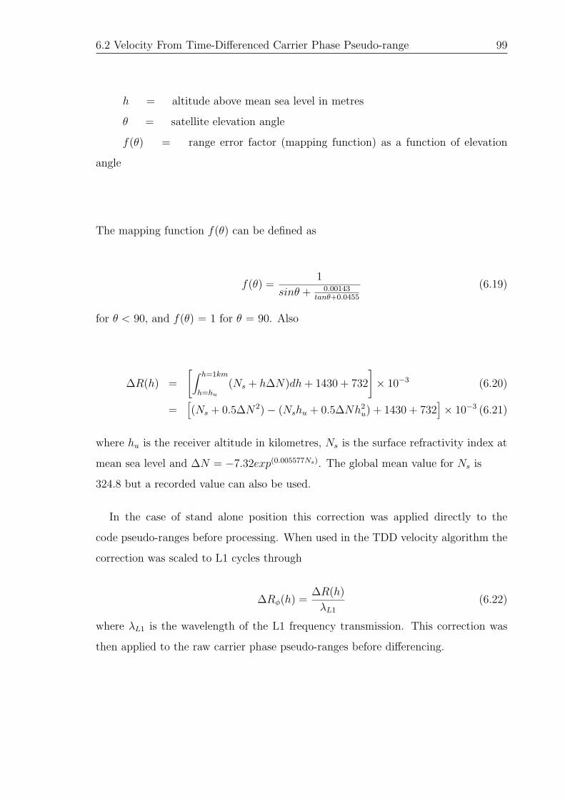
6.2 Velocity From Time-Differenced Carrier Phase Pseudo-range 99
h = altitude above mean sea level in metres
θ = satellite elevation angle
f(θ) = range error factor (mapping function) as a function of elevation
angle
The mapping function f(θ) can be defined as
f(θ) =1
sinθ + 0.00143tanθ+0.0455
(6.19)
for θ < 90, and f(θ) = 1 for θ = 90. Also
∆R(h) =
[∫ h=1km
h=hu
(Ns + h∆N)dh+ 1430 + 732
]× 10−3 (6.20)
=[(Ns + 0.5∆N2)− (Nshu + 0.5∆Nh2
u) + 1430 + 732]× 10−3 (6.21)
where hu is the receiver altitude in kilometres, Ns is the surface refractivity index at
mean sea level and ∆N = −7.32exp(0.005577Ns). The global mean value for Ns is
324.8 but a recorded value can also be used.
In the case of stand alone position this correction was applied directly to the
code pseudo-ranges before processing. When used in the TDD velocity algorithm the
correction was scaled to L1 cycles through
∆Rφ(h) =∆R(h)
λL1
(6.22)
where λL1 is the wavelength of the L1 frequency transmission. This correction was
then applied to the raw carrier phase pseudo-ranges before differencing.

6.2 Velocity From Time-Differenced Carrier Phase Pseudo-range 100
6.2.3.4 Ionospheric Correction
Ionospheric corrections were applied to the algorithm in two separate ways, dependent
on the mode of data collection. For dual frequency receivers the dual frequency data
was used to remove almost all of the ionospheric delay while for single frequency
receivers the Klobuchar (1996) ionospheric model was used.
The dual frequency data was corrected for ionospheric delay using observations on
both the L1 and L2 frequencies (Parkinson and Spilker, 1996a; GPS JPO, 1997; Misra
and Enge, 2004). The equation for this when using code pseudo-ranges was given in
equation 3.15 and this was used when estimating stand-alone position. In the TDD
velocity algorithm, however, carrier phase pseudo-range measurements were used and,
in this case, the equation can be represented as below.
IφL1 =φL1f1f2 − φL2f
22
f 22 − f 2
1
(6.23)
Use of dual frequency data removed almost all of the ionospheric delay that ap-
peared on the carrier phase pseudo-range observable on L1 although some residual
effects still remained. There was also some component of this correction that was
affected by receiver noise. Receiver noise was present on the carrier phase pseudo-
range observable and so was also present on IφL1. This manifested as high frequency
changes in the ionospheric delay, a notion which is empirically unsound. IφL1 was
therefore filtered through a low pass filter that removed much of the noise. This
process introduced a delay in the output of the TDD velocity algorithm through the
group delay of the filter, but this was considered unimportant since there was to be a
filter used to remove the drift from the eventual heave output, which will introduce
a larger group delay as described in §6.3. The low pass filter used was merely a
running average which took the mean of IφL1 for 24 epochs either side of the current
epoch. The smoothed dual frequency ionospheric correction had reduced noise and
so produced a less noisy TDD velocity output.
Ionospheric correction for single frequency data was provided by the Klobuchar
(1996) ionospheric model. This used a set of parameters, α and β, which each
contained four elements and were transmitted in the GPS navigation message. The

6.2 Velocity From Time-Differenced Carrier Phase Pseudo-range 101
algorithm used for this is given below.
The earth centred angle, ψ, was first calculated:
ψ =0.0137
(θ + 0.11)− 0.022 (6.24)
where θ is the satellite elevation angle.
Then the subionospheric latitude, λl could be computed:
λl = λ+ ψcosA (6.25)
where λ is the user receiver latitude and A is the satellite azimuth. Here the
maximum range of λl is ±0.416 such that if λl > 0.416, then λl = 0.416 and if
λl < −0.416, then λl = −0.416.
The subionospheric longitude, φl, was computed next:
φl = φ+
(ψsinA
cosλl
)(6.26)
where φ is user receiver longitude.
The geomagnetic latitude, λm, of the subionospheric location looking toward each
GPS satellite could then be calculated:
λm = λl + 0.064cos(φl − 1.617) (6.27)
Then local time, tl at the subionospheric point:
tl = 4.32× 10⁴φl +GPS time (6.28)
Now the slant factor, F , was calculated:

6.2 Velocity From Time-Differenced Carrier Phase Pseudo-range 102
F = 1.0 + 16.0× (0.53− θ)3 (6.29)
Then, the ionospheric time delay, Tiono was found by first computing the period of
model (PER) and subsequently x:
PER =3∑
n=0
βnλnm (6.30)
x =2π(tl − 50400)
PER(6.31)
Then Tiono could be computed from either
Tiono = F (5× 10⁻⁹) (6.32)
for |x| > 1.57. Or
Tiono = F
[5× 10⁻⁹ +
3∑n=0
αnφnm ×
(1− x2
2+x4
24
)](6.33)
The terms α and β in equations 6.33 and 6.30 respectively are those parameters
transmitted in the GPS navigation message.
As with tropospheric delay mitigation, this correction was applied directly to
code pseudo-ranges when stand-alone position was required. For the TDD velocity
algorithm the correction was scaled to L1 cycles, as described in equation 6.22 and
applied before differencing.
6.2.3.5 Correction for Satellite Loss
The nature of TDD velocity requires that two adjacent epochs of data are available
for each satellite to be used in the algorithm. If a satellite was lost below the elevation
mask then it was also removed from the observations of the previous epoch and as such
played no part in the estimation of TDD velocity. A similar technique was applied
to new satellites that appeared above the elevation mask in that they could not be
used in the TDD velocity algorithm until at least two adjacent epochs of data were
available.

6.2 Velocity From Time-Differenced Carrier Phase Pseudo-range 103
6.2.3.6 Cycle Slip Handling
The majority of cycle slips that may occur in the measurement of the carrier phase
pseudo-range observable are handled inherently as part of the TDD algorithm itself.
In order to difference the carrier phase pseudo-range observable across adjacent epochs
as described above, there had to be two consecutive epochs of data available to the
algorithm. When in the case of a particular satellite there were not consecutive
observations, that satellite’s data was discarded and not included in the algorithm for
that epoch. This applied when a satellite’s signal was lost for any reason and so did not
appear in the RINEX file, and also when it was regained and consequently reappeared.
Through this system the majority of cycle slips, which were caused through satellite
signal loss, were prevented from having an impact on the TDD velocity solution.
In addition to the cycle slip immunity offered by the TDD velocity algorithm, a
process of least squares analysis was developed that would remove any ‘bad’ obser-
vations that have been subject to slips and have introduced an error in the TDD
velocity estimation. After TDD processing the least squares residuals were analysed
and their mean value calculated. If a the residual of a particular observation was seen
to differ from the mean of the residuals by a sufficient amount then this observation
was removed from the system of equations and the least squares estimation computed
again.
Under the majority of circumstances this algorithm was sufficient to remove the
observation containing the cycle slip but, because the TDD algorithm differences car-
rier phase pseudo-ranges from seperate satellites, cycle slips were not always removed
in this way. In the TDD algorithm a reference satellite is chosen, the observations of
which are used to difference with the observations from the other usable satellites. If
the cycle slip occured on the observation from the reference satellite then all residuals
would be affected. In this instance the reference satellite observations were removed
from the algorithm, a new reference satellite was selected and the least squares
estimation computed again with the new reference satellite.
On rare occasions even this second attempt to provide cycle slip immunity was
not sufficient and under these circumstances it was considered that cycle slips had

6.2 Velocity From Time-Differenced Carrier Phase Pseudo-range 104
occured on multiple, possibly all, channels of the receiver. Algorithms exist to repair
these errors in carrier phase pseudo-range data but they have not been investigated as
part of this research. Instead, the epochs where this has occured have been removed
from the data set.
6.2.3.7 Carrier-to-Noise Density Weighting Scheme
Weighting schemes can be applied to the least squares processing of GPS observations
in order to weight more heavily any high quality observations and decrease the
influence of poor quality observations. These weighting schemes can improve the
quality of the position and velocity outputs produced from receiver raw observations,
particularly in the case of low cost receivers such as the U-Blox Antaris where tracking
loop componentry is of a low quality. In the case of low cost GPS receivers the
thermal noise and noise introduced by the code and carrier tracking loops due to low
quality componentry can be much more significant than that seen in higher grade
dual frequency receivers.
The use of the U-Blox Antaris low cost receiver in this thesis has necessitated the
development of a weighting scheme to better handle the raw carrier phase pseudo-
range observables. Weighting schemes have been suggested based upon both satellite
elevation angle and observation signal-to-noise ratio (Collins and Langley, 1999) but
analysis of the stand-alone position and TDD velocity residuals from the least squares
estimation using the U-Blox receiver suggested a strong correlation between poor
quality observations and carrier-to-noise density, C/N0. For this reason, and because
they are considered to be potentially more powerful, it was decided to employ a
weighting scheme based upon the carrier-to-noise density of each observation. Collins
and Langley (1999) implemented a weighting scheme based upon the approximation
of the formula for calculating carrier tracking loop noise given in Langley (1997).
σL1 =
√B
c/n0
· λL1
2π(6.34)
where σL1 is the error on the carrier phase measurement (m), B is the carrier tracking
loop bandwidth (Hz), c/n0 is the carrier-to-noise density expressed as a ratio (=10C/N0
10
in dB-Hz) and λL1 is the L1 carrier wavelength.
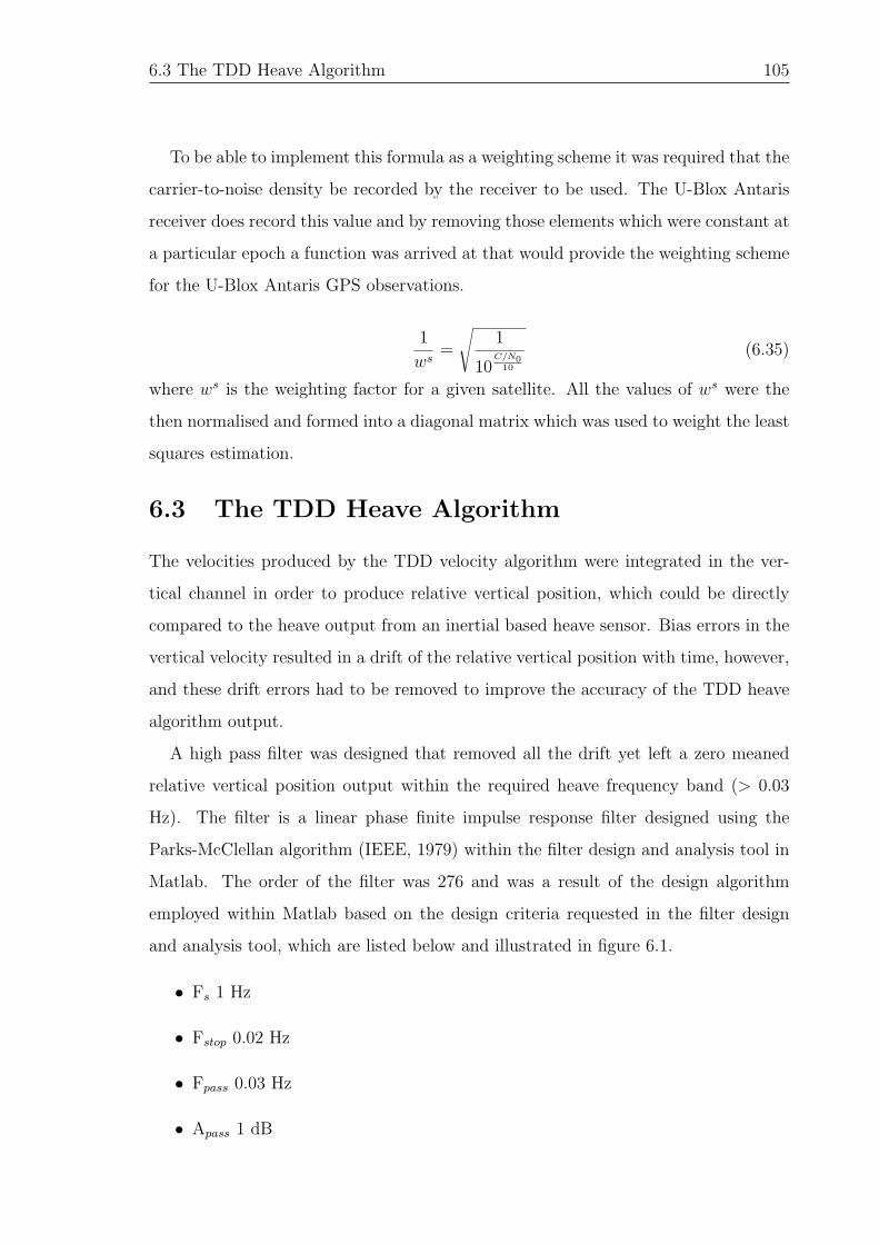
6.3 The TDD Heave Algorithm 105
To be able to implement this formula as a weighting scheme it was required that the
carrier-to-noise density be recorded by the receiver to be used. The U-Blox Antaris
receiver does record this value and by removing those elements which were constant at
a particular epoch a function was arrived at that would provide the weighting scheme
for the U-Blox Antaris GPS observations.
1
ws=
√1
10C/N0
10
(6.35)
where ws is the weighting factor for a given satellite. All the values of ws were the
then normalised and formed into a diagonal matrix which was used to weight the least
squares estimation.
6.3 The TDD Heave Algorithm
The velocities produced by the TDD velocity algorithm were integrated in the ver-
tical channel in order to produce relative vertical position, which could be directly
compared to the heave output from an inertial based heave sensor. Bias errors in the
vertical velocity resulted in a drift of the relative vertical position with time, however,
and these drift errors had to be removed to improve the accuracy of the TDD heave
algorithm output.
A high pass filter was designed that removed all the drift yet left a zero meaned
relative vertical position output within the required heave frequency band (> 0.03
Hz). The filter is a linear phase finite impulse response filter designed using the
Parks-McClellan algorithm (IEEE, 1979) within the filter design and analysis tool in
Matlab. The order of the filter was 276 and was a result of the design algorithm
employed within Matlab based on the design criteria requested in the filter design
and analysis tool, which are listed below and illustrated in figure 6.1.
• Fs 1 Hz
• Fstop 0.02 Hz
• Fpass 0.03 Hz
• Apass 1 dB

6.3 The TDD Heave Algorithm 106
• Astop -80 dB
Figure 6.1: High pass filter design criteria required by Matlab filter design and analysistool
The order of the filter was not considered an important factor when designing the
heave filter as the TDD heave algorithm was always intended to be a near real time
system. Increasing the performance of the filter in terms of its design criteria would
have the effect of increasing the filter order and, hence, the filter group delay. The
transfer function of the heave filter is shown in figure 6.2. It had a -3dB cut-off
frequency of 0.03 Hz and imparted a group delay of 138 samples on the heave output
data when GPS observables were recorded at 1 Hz.
The heave filter designed was used to remove all the drift from the relative position
output gained from the integration of the TDD velocities and the bias errors associated
with it.
A block schematic diagram of the full TDD heave algorithm is included here at
figure 6.3 showing the entire process from raw GPS data collection through to heave
output.

6.3 The TDD Heave Algorithm 107
Figure 6.2: Frequency and phase response of high pass heave filter
Figure 6.3: Block schematic diagram of the TDD heave algorithm

Chapter 7
The Spirent GSS7700 GPS/SBASSimulator Trials
7.1 Introduction
The IESSG has purchased a highly versatile piece of test equipment, called a Spirent
GSS7700 GPS/SBAS Simulator, that can simulate the entire GPS constellation and
generate signals that can be fed directly into a GPS receiver. The Spirent simulator
simulates the GPS signals transmitted by each of the GPS satellites as they would be
received by a GPS receiver that was undergoing the dynamics laid out in the simulator
scenario. As such, the Spirent simulator provides an excellent platform from which to
test different GPS receivers against one another and has been used extensively during
the development and testing of the TDD velocity algorithm discussed in chapter 6.
A trial was developed to assess the quality of the phase pseudo-range observable
recorded with a commercially available low cost GPS receiver, and its ability to be
used to estimate receiver velocity using the TDD velocity algorithm. A distinction was
drawn for the purposes of this trial between the TDD velocity algorithm, which uses
TDD to estimate receiver velocity, and the TDD heave algorithm, which integrates
the TDD velocity estimate and applies the high pass filter to produce a heave output.
The TDD velocity algorithm has been tested using three separate GPS receivers: one
low cost and two dual frequency. They have each been used to collect simulated
raw GPS observables under varying simulated dynamic conditions and the use of the
Spirent simulator allowed the extraction of truth data that meant a highly accurate
assessment of receiver performance was possible. The TDD heave algorithm has been
108

7.2 The Spirent GSS7700 GPS/SBAS Simulator 109
tested using a simulated marine scenario with dynamics close to those experienced
under real marine conditions.
This trial was the first to assess the performance of the TDD velocity and heave
algorithms using commercially available low cost GPS receivers under the controlled
conditions of a simulated environment. It has allowed an accurate assessment of
the ability of low cost receivers to provide a quality phase pseudo-range observable
and helped develop an understanding of the likely error sources, information vital
to the continued development of low cost receivers for accurate position and velocity
applications. This work expanded on the work already conducted in the estimation
of precise GPS velocity based on time differenced carrier phase pseudo-ranges using
a similar simulator (Ryan et al., 1997), which has tested a temporally differenced
carrier phase pseudo-range based velocity technique under various dynamics using
higher grade GPS receivers.
This chapter discusses the Spirent GSS7700 GPS/SBAS Simulator and the partic-
ular elements used in this project, the trial conducted on the simulator and goes on
to present the results of the trial.
7.2 The Spirent GSS7700 GPS/SBAS Simulator
The Spirent GSS7700 GPS/SBAS Simulator is a tool that provides a comprehen-
sive development and testing environment for satellite navigation hardware (Spirent,
2006). The Spirent simulator can simulate the environment experienced by a GPS
receiver while on a static or kinematic platform. The GPS transmitted signals can be
simulated and fed directly into an existing GPS receiver via an RF cable as though
that receiver where undergoing a set of predetermined vehicle dynamics, with full
control over a number of error sources.
The Spirent simulator can be considered to consist of two elements, a brief descrip-
tion of both is given in the following two subsections.
7.2.1 Simulator Hardware
The hardware purchased by the IESSG consists of two RF signal generators, a PC
and a pre-amp unit. A picture of the setup used in the simulator trial is given in

7.2 The Spirent GSS7700 GPS/SBAS Simulator 110
figure 7.1 and shows each of the main hardware elements required.
The signal generators generate and transmit the simulated GPS signals that will be
received at the receiver. Essentially, they convert the calculated pseudo-ranges into
the correct GPS messages from each satellite in view; the PC is used to configure the
signal generators using the SimGEN software explained in §7.2.2; and the pre-amp
has been designed to simulate the pre-amps that are found in many GPS antennas.
7.2.2 Simulator Software
SimGEN is the software that is provided as a development environment for the
designed simulations, termed scenarios. A set of description or source files go together
to define the scenario. The principle description files used during the simulator trial
were the motion file, which describes the motion of the receiver to be simulated, and an
atmosphere file that define what atmospheric effects are to be modelled. Navigation
data to describe satellite orbits can also be provided to the simulator so as to simulate
a particular date as accurately as possible.
The software uses the description files to run models that calculate such parameters
as pseudo-range, atmospheric delays and satellite position. Each of these parameters
can be output by the simulator, providing an excellent testbed for development of any
GPS navigation software.
7.2.3 Simulator Setup and Error Models
The Spirent simulator is tremendously versatile and gives the user complete control
over many of the error sources and accuracy parameters of the space section of the
GPS. For much of the trial all the error models that can be implemented using
the Spirent simulator were turned off as the simulator trial was primarily focussed
on isolating receiver based errors. Where atmospheric modelling was required the
STANAG (1990) model was used to impart tropospheric error on the simulated signals
and the Klobuchar (1996) model was used for ionospheric delay modelling. All other
models and error sources were turned off for the simulator trial but in future tests
the Spirent simulator could prove a powerful tool in the assessment of the impact of
various space segment based error sources on TDD velocity estimation using low cost

7.3 Trial Methodology 111
Figure 7.1: Spirent GNSS Simulator
receivers.
Satellite orbit information was provided to the simulator from a global RINEX
v2.1 navigation file for the simulated trial date downloaded from the CORS website
(National Geodetic Survey, 2007). This allowed a realistic simulation of the actual
conditions experienced on the day in terms of satellite availability. Satellite clock
offsets and drifts were also contained within the navigation file and modeled as such
within the simualtor.
7.3 Trial Methodology
The simulator trial was designed to test both the TDD velocity and heave algorithms
developed as part of the project, and the effect of the use of low cost receivers com-
pared to geodetic grade receivers. The hardware simulator, unlike software simulators,
produces simulated GPS signals that can be fed directly into real GPS receivers. This
allows a thorough assessment of receivers against each other as the errors introduced

7.3 Trial Methodology 112
by each can be isolated. With this in mind three separate types of receiver were
selected for the trials:
• Leica 530 Dual Frequency Receiver
• Novatel OEM4 Dual Frequency Receiver
• U-Blox Antaris LEA-4T Single Frequency Receiver
Each receiver was selected to represent a different section of the GPS receiver
market: the Leica 530 is a dual frequency geodetic receiver that is primarily used in
the land survey industry to record static observations, the Novatel OEM4 is another
dual frequency receiver that has been designed for the navigation market, and the U-
Blox Antaris is a single frequency low cost receiver that can record the carrier phase
pseudo-range observable.
Three scenarios were programmed into the Spirent simulator to test each receiver
under different dynamic conditions. Four trials where then designed that would
effectively test each receiver and also demonstrate the operability and limitations
of the TDD velocity and heave algorithms. An arbitrary date of 24 January 2006 was
selected to be the trial date for all simulator trials and the ephemeris data for that
date, downloaded from National Geodetic Survey (2007), was loaded into each of the
three scenarios.
An auxiliary trial, trial 5, is also included here although it did not involve the use
of the Spirent simulator but rather the collection of real GPS data.
7.3.1 The Simulated Scenarios
Three scenarios were developed and programmed into the Spirent simulator. These
were designed to test the algorithm under different dynamics and are outlined below.
7.3.1.1 Static
The static scenario simulated a static GPS receiver at the same location as a real
GPS antenna sited on the turret of the IESSG building. The position of the simulated
receiver was programmed into SimGEN as

7.3 Trial Methodology 113
• Latitude: 52 56′ 26.49612′′N
• Longitude: 1 11′ 32.32482′′W
• Height: 98.47 m
7.3.1.2 Marine
A marine scenario was developed that was intended to deliver the most realistic
simulation of the intended algorithm environment. A motion file was programmed
into the simulator using SimGEN. The motion file held the vessel static, in the same
position as simulated for the static scenario, for a period of 650 s so that each of the
GPS receivers used would have sufficient time to lock on to all the satellites before
and simulated motion began. The scenario then took the simulated vessel from the
start position in a straight line in a north-westerly direction for a further 1,150 s.
Over the course of the simulation four separate sea states of varying severity were
simulated. SimGEN only allows for sinusoidal heave motion within the sea state file
and so realistic heave motion cannot be simulated but the principles of heave motion
remain the same. Therefore, during the marine scenario the TDD velocities computed
using the three separate receivers were used to create a heave plot of vertical motion,
which was compared directly to heave derived from true vertical motion.
A plan view of the trajectory of the marine scenario is shown in figure 7.2 and the
height profile can be seen in figure 7.3. Whilst the height profile plot in figure 7.3 does
not clearly show the frequency of the heave in each of the separate sea state zones
the details of each sea state are given in table 7.1. In addition to the trajectory of
the marine scenario, it is also necessary to include the velocity profile, seen in figure
7.4, which shows the changes in North, East and Down velocity with time during the
scenario.
Sea State Wave Height (m) Wave Frequency (Hz)1 1.5 0.42 1.5 0.23 1.5 0.14 1.5 0.05
Table 7.1: Table of sea states used in simulated marine scenario

7.3 Trial Methodology 114
Figure 7.2: Plan view of simulated marine scenario trajectory
Figure 7.3: Height profile of simulated marine scenario

7.3 Trial Methodology 115
Figure 7.4: Velocity profile of simulated marine scenario
7.3.1.3 High Dynamics
In order to test the dynamic stress performance of the signal tracking loops on
each receiver a high dynamic scenario was designed. This used the aircraft vehicle
model within SimGEN and subjected the simulated aircraft to rapid accelerations
and changes of direction. The high dynamics scenario began at the same position as
that detailed in §7.3.1.1, which was the position for the static trial. This position was
held for 300 s to allow each receiver to lock on to all satellites before high dynamic
motion began. A series of accelerations, turns and climbs were then initiated over the
course of the simulation. A plan view of the simulated high dynamics trajectory is
given in figure 7.5 and the height profile is shown in figure 7.6. The velocity profile is
also included in figure 7.7.
7.3.2 The Trials
The three scenarios were designed to test the algorithm and receivers under differ-
ent dynamics; a series of trials were developed to isolate receiver based errors and
demonstrate the functionality of the TDD velocity and heave algorithms. The trials

7.3 Trial Methodology 116
Figure 7.5: Plan view of simulated high dynamics scenario
Figure 7.6: Height profile of simulated high dynamics scenario

7.3 Trial Methodology 117
Figure 7.7: Velocity profile of simulated high dynamics scenario
are numbered one to five and each had a specific objective, which is set out in the
following subsections.
7.3.2.1 Trial 1: Receiver Test
Trial one was designed to isolate and quantify errors specific to the particular receiver
used during data collection. In order to achieve this all errors controllable within
SimGEN were turned off and pure geometric range data was fed from the simulator
into each receiver. Therefore any raw observables recorded only displayed errors
introduced by the receiver.
It was suspected that each receiver would behave differently dependent on the
dynamics to which it was subjected and the setup of the signal tracking loops within
receiver firmware. It was therefore decided that each receiver should record data from
all three scenarios in turn, resulting in three separate tests within trial one.
• Static Test: comparison of TDD GPS velocity from all three receivers while
subjected to the static scenario with all errors turned off.
• Marine Test: comparison of TDD GPS heave from all three receivers while
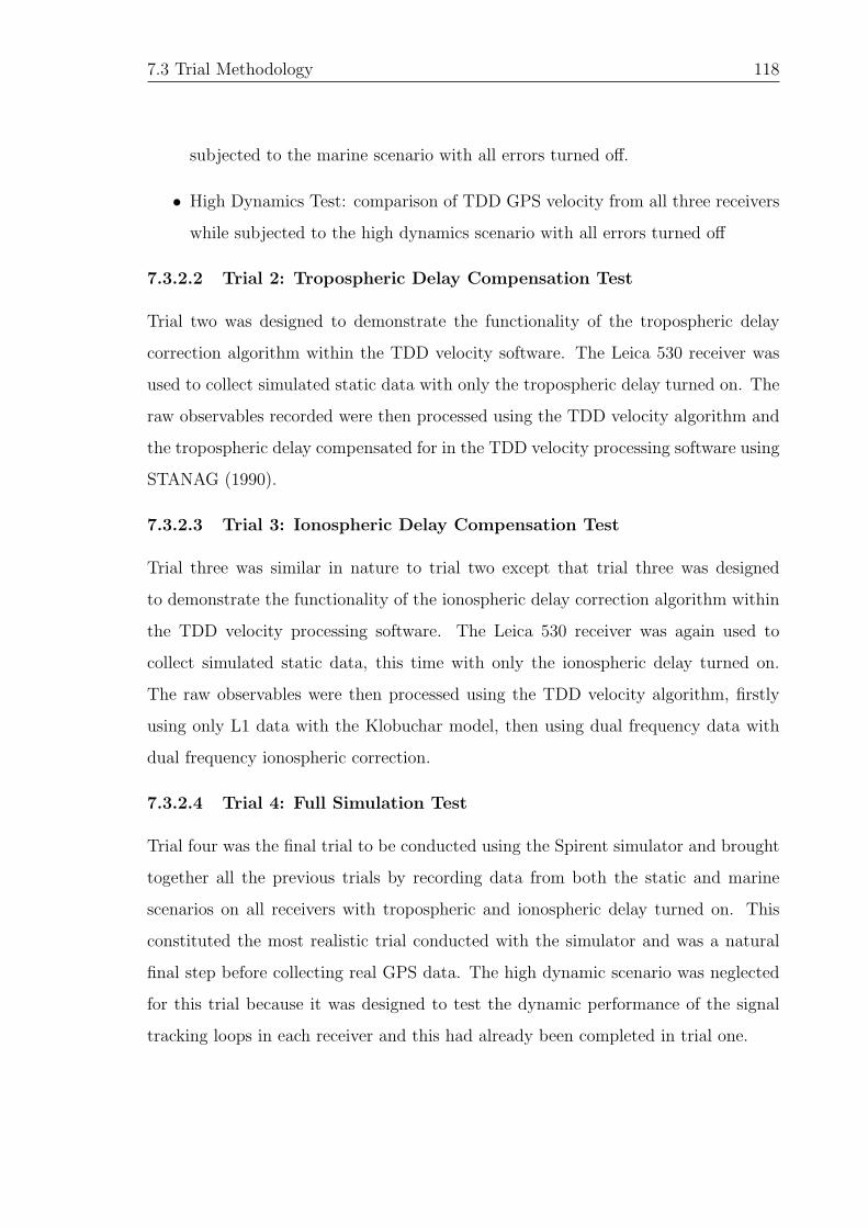
7.3 Trial Methodology 118
subjected to the marine scenario with all errors turned off.
• High Dynamics Test: comparison of TDD GPS velocity from all three receivers
while subjected to the high dynamics scenario with all errors turned off
7.3.2.2 Trial 2: Tropospheric Delay Compensation Test
Trial two was designed to demonstrate the functionality of the tropospheric delay
correction algorithm within the TDD velocity software. The Leica 530 receiver was
used to collect simulated static data with only the tropospheric delay turned on. The
raw observables recorded were then processed using the TDD velocity algorithm and
the tropospheric delay compensated for in the TDD velocity processing software using
STANAG (1990).
7.3.2.3 Trial 3: Ionospheric Delay Compensation Test
Trial three was similar in nature to trial two except that trial three was designed
to demonstrate the functionality of the ionospheric delay correction algorithm within
the TDD velocity processing software. The Leica 530 receiver was again used to
collect simulated static data, this time with only the ionospheric delay turned on.
The raw observables were then processed using the TDD velocity algorithm, firstly
using only L1 data with the Klobuchar model, then using dual frequency data with
dual frequency ionospheric correction.
7.3.2.4 Trial 4: Full Simulation Test
Trial four was the final trial to be conducted using the Spirent simulator and brought
together all the previous trials by recording data from both the static and marine
scenarios on all receivers with tropospheric and ionospheric delay turned on. This
constituted the most realistic trial conducted with the simulator and was a natural
final step before collecting real GPS data. The high dynamic scenario was neglected
for this trial because it was designed to test the dynamic performance of the signal
tracking loops in each receiver and this had already been completed in trial one.
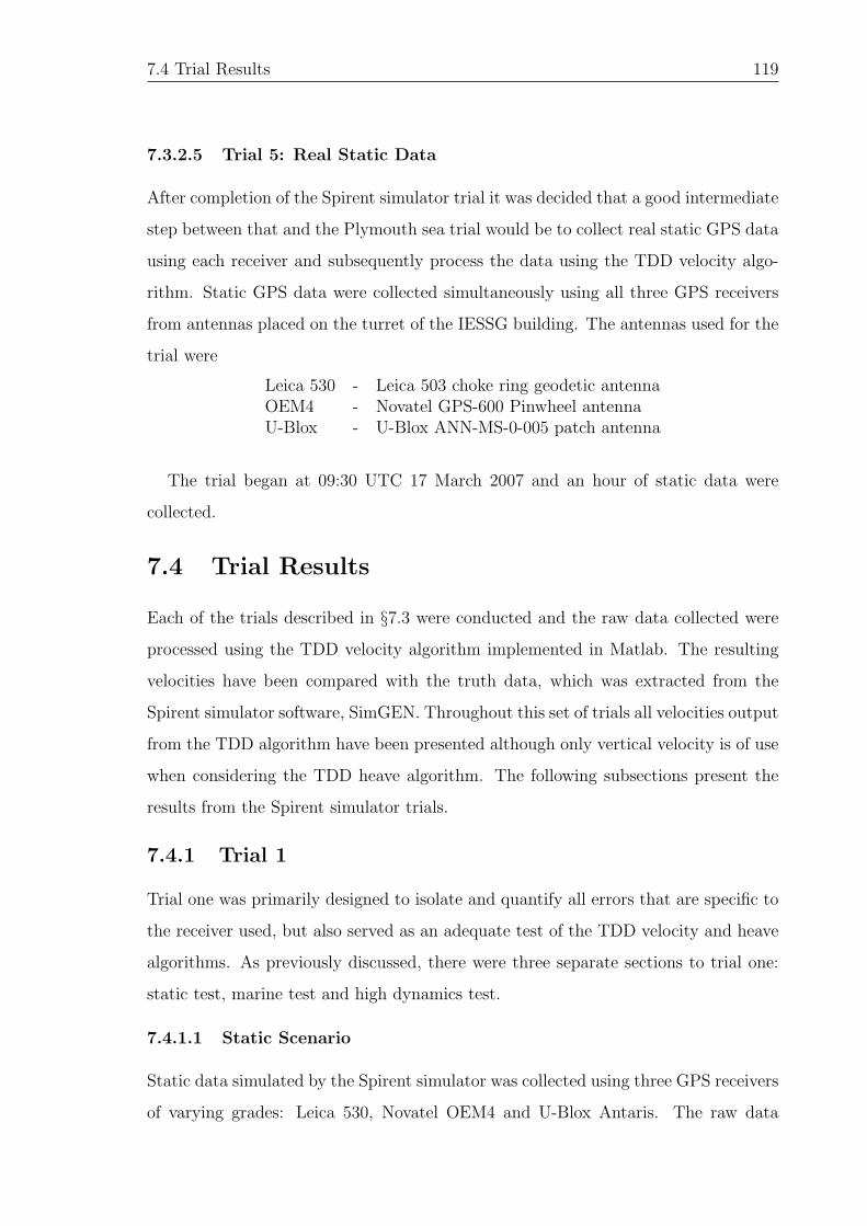
7.4 Trial Results 119
7.3.2.5 Trial 5: Real Static Data
After completion of the Spirent simulator trial it was decided that a good intermediate
step between that and the Plymouth sea trial would be to collect real static GPS data
using each receiver and subsequently process the data using the TDD velocity algo-
rithm. Static GPS data were collected simultaneously using all three GPS receivers
from antennas placed on the turret of the IESSG building. The antennas used for the
trial were
Leica 530 - Leica 503 choke ring geodetic antennaOEM4 - Novatel GPS-600 Pinwheel antennaU-Blox - U-Blox ANN-MS-0-005 patch antenna
The trial began at 09:30 UTC 17 March 2007 and an hour of static data were
collected.
7.4 Trial Results
Each of the trials described in §7.3 were conducted and the raw data collected were
processed using the TDD velocity algorithm implemented in Matlab. The resulting
velocities have been compared with the truth data, which was extracted from the
Spirent simulator software, SimGEN. Throughout this set of trials all velocities output
from the TDD algorithm have been presented although only vertical velocity is of use
when considering the TDD heave algorithm. The following subsections present the
results from the Spirent simulator trials.
7.4.1 Trial 1
Trial one was primarily designed to isolate and quantify all errors that are specific to
the receiver used, but also served as an adequate test of the TDD velocity and heave
algorithms. As previously discussed, there were three separate sections to trial one:
static test, marine test and high dynamics test.
7.4.1.1 Static Scenario
Static data simulated by the Spirent simulator was collected using three GPS receivers
of varying grades: Leica 530, Novatel OEM4 and U-Blox Antaris. The raw data

7.4 Trial Results 120
collected were then converted into RINEX v2.1 files ready for processing through the
TDD velocity algorithm. The velocities output by the algorithm are shown in figures
7.8, 7.9 and 7.10 for Leica 530, Novatel OEM4 and U-Blox Antaris respectively. The
data collected was from a static scenario and the plots of TDD velocity can therefore
also be considered error plots. The error can be shown to be normally distributed and
so the standard deviation of the error is presented in table 7.2; the mean of the error
experienced during the static scenario was at the micrometre or tens of micrometer
level and so was considered negligible and not included in the results of table 7.2.
Table 7.2 shows that the U-Blox receiver performed to the same standard as both
the dual frequency receivers when in a static environment. The figures presented in
the table show standard deviation and mean error values for the U-Blox receiver of the
same order as for the Leica and the Novatel. These results were slightly unexpected
considering the difference in cost between the receivers but were thought to probably
be an artefact of the tracking loop algorithms employed in the U-Blox receiver. It is
accepted that the Leica and Novatel will most likely utilize higher grade componentry
within the receiver, but when static the U-Blox receiver may be able to use the lack
of dynamics to alter the bandwidth of its tracking loops. This analysis is largely
conjecture but it is certainly safe to say from these results that, under static error
free conditions, the U-Blox receiver can perform at least as well as the Leica and
Novatel receivers.
Receiver 1σ Standard Dev. (mm/s)Type North East DownLeica 530 0.8 0.7 2.0OEM4 0.7 0.6 1.6U-Blox 0.8 1.0 3.4
Table 7.2: Results of static test of TDD velocity algorithm using error free simulateddata
7.4.1.2 Marine Scenario
The marine scenario was designed to test the TDD heave algorithm in an environment
that would be as close as possible to the intended environment of use. Error free data
were once again collected using the same three receivers, this time being subjected to a

7.4 Trial Results 121
Figure 7.8: Leica 530 dual frequency receiver TDD velocity from simulated static
Figure 7.9: Novatel OEM4 dual frequency receiver TDD velocity from simulated staticdata

7.4 Trial Results 122
Figure 7.10: U-Blox Antaris single frequency receiver TDD velocity from simulatedstatic data
simulated marine environment. These data were then processed using the TDD heave
algorithm as in the static test and the results compared to a heave output created
from the true marine height profile seen in figure 7.4. This was done by simply passing
the truth height data through the same high pass filter that was used to remove drift
from the integrated TDD vertical velocities in the heave algorithm.
When the velocity profiles produced using data from each receiver were compared
to the true velocity profiles extracted from SimGEN, the results showed characteristics
largely similar to those demonstrated in the following analysis of positional heave data.
This trial was designed to test the TDD heave algorithm but, as the TDD heave
algorithm is based on velocity estimates, the results for positional heave expressed
below apply equally well for TDD velocity.
A strong correlation was seen between the truth height data and the relative
height data produced through the integration of TDD velocities. Figure 7.11 shows
the difference plot of the true height and integrated TDD velocity using Leica 530
dual frequency data; the bias of 98.470 m on the truth height was removed for this
comparison. The results in figure 7.11 clearly show the drift on the integrated TDD

7.4 Trial Results 123
Figure 7.11: Leica 530 integrated TDD position drift error from the marine scenario
velocity caused by bias errors in velocity estimation. This drift was removed by passing
the integrated TDD velocity through the high pass filter designed for the TDD heave
algorithm and detailed in §6.3. Figure 7.12 shows a comparison between high pass
filtered true height and high pass filtered integrated Leica 530 TDD velocity and it
can be seen that the drift was removed by the filter; the results gained from data
collected with the Novatel OEM4 and U-Blox Antaris GPS receivers can be seen in
figures 7.13 and 7.14 respectively.
A bias was seen on the error plot of approximately 6 mm, which was caused by a
residual left after the high pass filtering of the true height data. The high pass filter
has finite stop band attenuation of -80 dB and so a residual height will remain after
filtering. This hypothesis was proven using the formula to calculate gain in dB:
A = 20log(S1
S2
)(7.1)
where A is the gain in dB and S1 and S2 are the levels of the signals. Setting the
values of S2 = 98.470 m and S1 = 6 mm yields a gain of -84 dB, which is very close
to the stop band attenuation of the high pass filter.
It can be seen from the error plots in figures 7.12, 7.13 and 7.14 that, when subjected
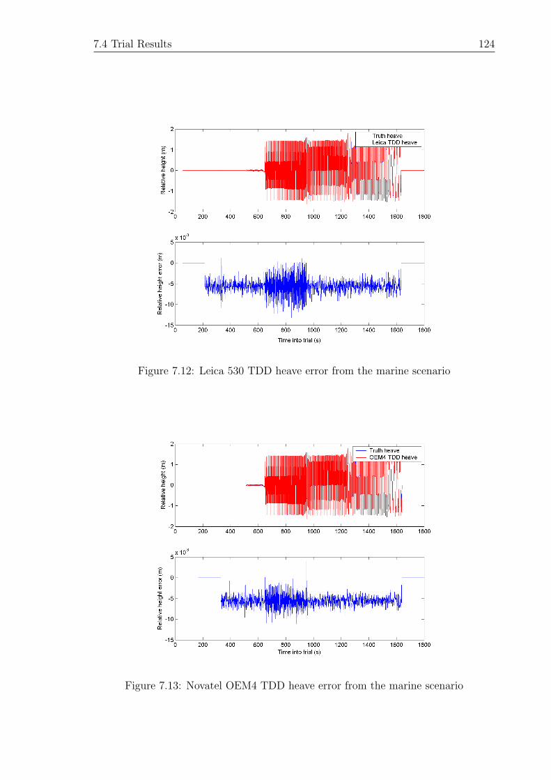
7.4 Trial Results 124
Figure 7.12: Leica 530 TDD heave error from the marine scenario
Figure 7.13: Novatel OEM4 TDD heave error from the marine scenario

7.4 Trial Results 125
Figure 7.14: U-Blox Antaris TDD heave error from the marine scenario
to a dynamic scenario, the Leica and Novatel receivers clearly outperformed the U-
Blox receiver with errors which appeared over an order of magnitude smaller under
visual inspection. It was also noted that the areas which contained the largest error
on all the vertical velocity error plots coincided with the time when the receiver was
subjected to the highest frequency of motion. Table 7.3 shows the errors in the TDD
heave from each receiver when subjected to the various sea states during the trial.
The high level of performance of the Novatel and Leica dual frequency receivers
suggested that there was no catastrophic failure in the TDD heave algorithm. It was
therefore assumed that the large errors seen in the results of the U-Blox receiver were
caused by the receiver itself and, more specifically, the receiver tracking loops. The
results in table 7.3 show that the errors in the TDD heave from the U-Blox receiver
were much greater than those seen in the Leica and Novatel receivers during sea state
one yet they quickly reduced to levels of a similar magnitude when the frequency
of motion was decreased during the remaining sea states. The TDD heave errors
experienced by the U-Blox receiver during sea states three and four were no different
to those seen when using the Leica and Novatel. A plot of the magnitude of the
accelerations simulated in the Spirent simulator during the marine trial can be seen in

7.4 Trial Results 126
figure 7.15 and the peak and mean accelerations during the trial are presented in table
7.4. Correlation of table 7.4 with table 7.3 gives an indication of what level of receiver
induced error can be expected due to dynamic stress and suggests that degradation
of performance of the U-Blox receiver began to be significant when accelerations of
approximately 3 m/s2 were experienced.
Leica 530 Nov OEM4 U-Blox AntarisSea State std (1σ) mean std (1σ) mean std (1σ) mean
(mm) (mm) (mm) (mm) (mm) (mm)1 3.4 -5.6 2.6 -5.5 70.4 -4.42 1.4 -5.6 1.2 -5.5 6.4 -6.23 1.2 -5.6 1.1 -5.7 0.9 -5.604 1.4 -5.6 1.4 -5.9 0.82 -5.6
Table 7.3: Receiver induced heave errors for each section of the simulated marinescenario
Sea State Mean Acceleration (m/s2) Peak Acceleration (m/s2)1 5.993 9.4572 1.510 3.6003 0.379 0.9224 0.095 0.232
Table 7.4: Mean accelerations simulated during the marine trial
Frequency analysis of the error experienced in TDD heave from each of the U-Blox
receiver showed that the large errors seen were strongly linked to the frequency of
motion experienced by the receiver at higher frequencies. The FFT of the error in
U-Blox TDD heave can be seen in figure 7.16 where each plot relates to the FFT
of a separate section of the scenario during which the receiver was subjected to a
particular frequency of vertical motion. The frequency analysis shown in figure 7.16
clearly shows that the error occurred at the frequency of motion experienced by the
receiver as the spikes in the FFT data occur at 0.4 Hz, 0.2 Hz and 0.1 Hz, the same
frequencies of motion used in the marine scenario. Once frequency of motion has
dropped to 0.05 Hz the power in the error signal at that frequency appears to have
dropped below the noise level and so has little effect on the error. It can also be
seen in the figure 7.16 that the Gaussian noise was of a greater magnitude when the
receiver experienced the higher frequencies of motion.

7.4 Trial Results 127
It was clear from these results that the errors introduced by the U-Blox receiver
when in motion were far larger than those introduced by either the Leica or the
Novatel. These errors included a Gaussian component and a component that occurred
at the frequency of motion with both components seen regardless of the receiver used.
The largest errors occurred when the receiver was subjected to the highest frequencies
of motion (in this trial a sinusoidal motion at 0.4 Hz saw the largest magnitude of
error) and consequently when the signal tracking loops within the receiver are placed
under the most dynamic stress. It was the dynamic stress that was thought to cause
that error in the heave estimate which occurs at the frequency of motion. The extra
dynamic stress on the carrier tracking loop was handled more easily in the receivers
with higher grade componentry than in the U-Blox. It is believed that the relatively
sluggish dynamic performance of the U-Blox receiver caused a significant lag in the
output of the carrier tracking loop, and resulted in the heave error at the frequency
of motion. Also, as discussed in §3.3.4, it was thought that the increased receiver
dynamics resulted in an increase in carrier tracking loop bandwidth in order to track
the GPS signals, which had an adverse effect on carrier tracking loop noise.
The true cause of the dynamic stress error at the firmware level is difficult to
appreciate fully but it can certainly be surmised from the results obtained that higher
accelerations, which place the receiver tracking loops under greater dynamic stress,
cause errors in the U-Blox receiver that can be more than an order of magnitude
greater than those seen in either of the dual frequency receivers.
7.4.1.3 High Dynamic Scenario
The high dynamic scenario was designed to place the signal tracking loops under far
greater dynamic stress than in the marine test. This would endorse the findings of
the marine test and give an idea of the magnitude of error that may occur when using
the TDD velocity algorithm in more dynamic applications.
The TDD velocities calculated using the raw observables from each receiver were
compared to the velocities extracted from the simulator truth file. The error plots
based on velocities from each of the three receivers can be seen in figures 7.17, 7.18
and 7.19.

7.4 Trial Results 128
Figure 7.15: Magnitude of simulated vessel acceleration during the marine trial
Figure 7.16: Frequency analysis of error in U-Blox Antaris TDD velocity duringmarine trial

7.4 Trial Results 129
Figure 7.17: Leica 530 dual frequency receiver induced velocity error from simulatedhigh dynamics data
The error seen for both the Leica and the Novatel was found to have a normal
distribution with a few outliers that, through visual inspection, can be seen to coincide
with some of the large accelerations induced as part of the high dynamics scenario.
The errors associated with these large accelerations occur due to the excessive stress
placed on the carrier tracking loop within the receivers but in both the Leica and
Novatel receivers, normally distributed errors followed quickly after constant velocity
was resumed.
The error for the U-Blox receiver seen in figure 7.19 shows much more prominent
errors that also coincide with the times of the large accelerations in the scenario, which
are around an order of magnitude greater than those seen from either the Leica or the
Novatel. During the periods of the scenario when constant velocity was experienced
the error in the U-Blox receiver is normally distributed but the time required for this
is greater than with the higher grade receivers.

7.4 Trial Results 130
Figure 7.18: Novatel OEM4 dual frequency receiver induced error from simulated highdynamics data
Figure 7.19: U-Blox Antaris single frequency receiver induced error from simulatedhigh dynamics data

7.4 Trial Results 131
7.4.2 Trial 2
Trial two was test to confirm the functionality of the tropospheric correction used in
the TDD velocity algorithm and also to give an idea of the magnitude of the error
that may be seen in the TDD velocity estimation due to unmitigated tropospheric
effects. Static data was collected using the Leica 530 receiver only, this time with
the tropospheric error modeled within SimGEN using the STANAG (1990). This
error was then compensated for within the TDD velocity algorithm using the same
algorithm. The magnitude of the errors seen in the uncompensated TDD velocity
solution showed the likely errors caused by unmitigated tropospheric effects, and the
functionality of the tropospheric compensation within the TDD velocity algorithm
was demonstrated in the compensated TDD velocity estimation.
Two sets of TDD processed velocities from simulated static data with tropospheric
error modeling turned on and collected using a Leica 530 can be seen in figures 7.20 and
7.21. Figure 7.20 shows the velocities with no tropospheric correction applied during
processing and it is clear from these plots that the rate of change of the troposphere
can be a significant source of error and must be mitigated within the TDD velocity
algorithm. Figure 7.21 shows the same data processed with the STANAG (1990)
tropospheric model applied and shows a plot with bias error removed.
The results presented in figures 7.20 and 7.21 are summarized in table 7.5. The
figures for the error in the TDD velocity when tropospheric delay remained uncom-
pensated were greater than those seen when the STANAG (1990) tropospheric model
was employed in the TDD velocity algorithm. The uncompensated figures did not
show a great deal of extra error but the statistical analysis hid bias errors of ±2
mm/s in horizontal velocity and ±4 mm/s in vertical velocity. The figures for the
TDD velocity when tropospheric delay compensation was employed compared very
well with the static error free figures presented in table 7.2 from trial one. This
was expected as the TDD algorithm employed the same tropospheric model as the
simulator but did prove the functionality of this algorithm employed in the Matlab
code.

7.4 Trial Results 132
Tropospheric 1σ Standard Dev. Mean ErrorCompensation (mm/s) (mm/s)Method N E D N E DUncompensated 1.2 1.0 2.6 -0.2 -0.6 0.3STANAG 0.7 0.8 1.9 0.0 0.0 0.0
Table 7.5: Leica 530 TDD velocity error for static data with tropospheric delaymodeled
Figure 7.20: Leica 530 TDD velocities from simulated static data with troposphericerror modeled and no correction applied
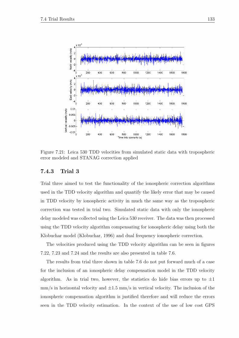
7.4 Trial Results 133
Figure 7.21: Leica 530 TDD velocities from simulated static data with troposphericerror modeled and STANAG correction applied
7.4.3 Trial 3
Trial three aimed to test the functionality of the ionospheric correction algorithms
used in the TDD velocity algorithm and quantify the likely error that may be caused
in TDD velocity by ionospheric activity in much the same way as the tropospheric
correction was tested in trial two. Simulated static data with only the ionospheric
delay modeled was collected using the Leica 530 receiver. The data was then processed
using the TDD velocity algorithm compensating for ionospheric delay using both the
Klobuchar model (Klobuchar, 1996) and dual frequency ionospheric correction.
The velocities produced using the TDD velocity algorithm can be seen in figures
7.22, 7.23 and 7.24 and the results are also presented in table 7.6.
The results from trial three shown in table 7.6 do not put forward much of a case
for the inclusion of an ionospheric delay compensation model in the TDD velocity
algorithm. As in trial two, however, the statistics do hide bias errors up to ±1
mm/s in horizontal velocity and ±1.5 mm/s in vertical velocity. The inclusion of the
ionospheric compensation algorithm is justified therefore and will reduce the errors
seen in the TDD velocity estimation. In the context of the use of low cost GPS

7.4 Trial Results 134
Ionospheric 1σ Standard Dev. Mean ErrorCorrection (mm/s) (mm/s)Method N E D N E DUncompensated 0.8 0.7 2.1 0.1 -0.3 0.8Klobuchar 0.8 0.7 2.0 0.1 0.2 -0.2Dual Frequency 0.8 0.7 2.0 0.1 0.1 0.8
Table 7.6: Standard deviation and mean error using Klobuchar and dual frequencyionospheric correction
Figure 7.22: TDD processed simulated static data with ionosphere modeled and nocorrection applied
receivers for the estimation of TDD heave as is used throughout this thesis, the errors
associated with single frequency data collection can be expected to be reasonably
small and not to give too great a disadvantage.
7.4.4 Trial 4
As a final trial using the simulator data was collected using all three receivers from
both the static and marine scenarios with both ionospheric and tropospheric errors
modeled. This was thought to be a good final test of the TDD algorithm before the
collection and processing of real GPS data. In this trial the TDD velocities seen during
the static scenario are presented but, as in trial one, the marine scenario analysis is

7.4 Trial Results 135
Figure 7.23: TDD processed simulated static data with ionosphere modeled andKlobuchar correction applied
Figure 7.24: TDD processed simulated static data with ionosphere modeled and dualfrequency correction applied

7.4 Trial Results 136
Receiver 1σ Standard Dev. (mm/s)Type N E DLeica 530 0.8 0.7 2.0OEM4 0.6 0.6 1.6U-Blox 0.6 0.7 1.5
Table 7.7: Standard deviation and mean error of TDD processed simulated staticdata with tropospheric and ionospheric correction
conducted on the TDD heave output.
The TDD processed velocity errors are presented in table 7.7 for the static scenario
and table 7.8 for the marine scenario. The mean error results were all negligible for
the static scenario and so were not included in table 7.7. It is accepted that the error
for the marine scenario will not exhibit a normal distribution and that errors will be
larger during separate sections of the marine simulation due to the errors highlighted
by the analysis in §7.4.1.2 and so errors are expressed for each section of the scenario
individually.
The results for the static scenario show a strong correlation with the static scenario
results seen in trial one. Each receiver had TDD processed velocity errors of a
similar magnitude showing that, under static conditions, all receivers had similar
performance.
The results for the marine scenario again substantiate the findings of trial one and
show that the U-Blox receiver was outperformed by both the Leica and the Novatel
receivers under dynamic conditions. The results show a striking resemblance to those
from the marine scenario in trial one.
Leica 530 Nov OEM4 U-Blox AntarisSea State std (1σ) mean std (1σ) mean std (1σ) mean
(mm) (mm) (mm) (mm) (mm) (mm)1 2.5 -5.6 2.5 -5.6 76.1 -5.62 1.4 -5.6 1.7 -5.5 6.5 -5.43 2.1 -5.6 1.6 -5.5 2.1 -5.64 2.2 -5.6 1.8 -5.8 2.4 -5.8
Table 7.8: Standard deviation and mean error of TDD processed simulated marinedata with tropospheric and ionospheric correction

7.5 Spirent Simulator Trial Summary 137
7.4.5 Trial 5
Trial five has been added to this chapter although it did not involve use of the
Spirent simulator. It was designed as an interim trial between data collected on
the simulator and data collected during the sea trial, discussed in chapter 8. Static
data was recorded using all three receivers from the turret on the IESSG building.
Now that the simulator was no longer in use antennas were required for each receiver.
It was decided that the antennas used in the sea trial would also be used in this static
trial so as to gain an idea of the accuracy of the each receiver/antenna combination.
The results of trial 5 can be seen in table 7.9, and the plots of TDD velocity from
each of the three receivers is displayed in figures 7.25, 7.26 and 7.27.
The results shown in table 7.9 agree very strongly with the results shown for trials
one and four, conducted with the Spirent simulator. Each antenna appeared able to
record raw observations that, when processed through the TDD velocity algorithm,
resulted in velocity errors of a similar magnitude. The TDD velocity algorithm was
capable of estimating receiver velocity at the mm/s level under static conditions using
any of the receivers.
The results of this trial endorse the results of trial three, which suggested that
ionospheric effects would have little effect on the TDD velocity algorithm performance.
In this trial the U-Blox low cost single frequency receiver has performed as well as
the dual frequency Leica and Novatel receivers. Thus, there is little benefit from the
use of dual frequency receivers when in use with the TDD velocity algorithm.
Receiver 1σ Standard Deviation (m/s) Mean Error (m/s)Type N E D N E DLeica 530 1.9 1.5 3.4 0.0 0.1 -0.2OEM4 2.0 1.8 3.8 0.0 0.2 -0.1U-Blox 1.8 1.1 3.6 0.3 0.1 0.6
Table 7.9: Standard deviation and mean error of TDD processed static GPS data
7.5 Spirent Simulator Trial Summary
The simulator trials and the collection of real static GPS data have been a strong aid
in the development of the TDD velocity algorithm, the discovery of its limitations and

7.5 Spirent Simulator Trial Summary 138
Figure 7.25: TDD processed static GPS collected using Leica 530 dual frequencyreceiver
Figure 7.26: TDD processed static GPS data collected using OEM4 dual frequencyreceiver

7.5 Spirent Simulator Trial Summary 139
Figure 7.27: TDD processed static GPS data collected using U-Blox Antaris singlefrequency receiver
for analysis of the effects of the use of low cost receivers compared to dual frequency
geodetic receivers.
Trial one used simulated, error free, data collected using each of the three receivers
and three scenarios to test the effects of the receiver on the accuracy of TDD processed
velocity and TDD processed heave. Results of the static scenario showed that under
static conditions the U-Blox receiver performed to the same standard as the Leica
and Novatel receivers. During the marine scenario, however, the U-Blox receiver
was unable to cope with the same level of dynamic stress as the Leica and Novatel,
although the accelerations experienced were very high. Under simulated marine
dynamics the noise introduced by the U-Blox increased by approximately an order of
magnitude at very high accelerations and performance began to deviate significantly
from the performance of the other two receivers at accelerations of around 3 m/s2.
These results were substantiated by a further high dynamics test.
Trial two collected simulated static data with tropospheric delay only modeled in
SimGEN. The data were collected using only the Leica 530 receiver and then processed
through the TDD velocity algorithm where the STANAG tropospheric model was

7.5 Spirent Simulator Trial Summary 140
used to compensate for tropospheric delay. The results showed that uncompensated
tropospheric delay error can produce bias errors in the order of ±2 mm/s in horizontal
velocity and ±4 mm/s in vertical velocity and, as such, should be compensated
for. The results for the tropospheric delay compensated TDD velocities showed the
tropospheric delay compensation algorithm to be working effectively.
Trial three was similar in nature to trial two but this time tested the functionality
of the ionospheric compensation algorithms for both single and dual frequency re-
ceivers and the magnitude of error in the TDD velocity estimation due to ionospheric
activity. Simulated static data were collected, again using the Leica 530, with only
ionospheric delay modeled within SimGEN using the Klobuchar model. The data
were then processed using the TDD velocity algorithm and both the Klobuchar and
dual frequency ionospheric correction algorithms used to compensate for ionospheric
delay. The results showed that ionospheric effects could be expected to have an effect
on TDD velocity estimates of up to ±1 mm/s in horizontal velocity and ±1.5 mm/s
in vertical velocity. This level of error justified the inclusion of compensation models
in the TDD velocity algorithm but did suggest that the use of single frequency data
from low cost GPS receivers would have little effect on overall velocity accuracy using
the TDD velocity algorithm. Trial three also showed both algorithms to be effective in
the removal of ionospheric delay. A simulator based anomaly was that the Klobuchar
model performed equally as well as the dual frequency algorithm due to the fact that
the model applied in SimGEN is Klobuchar. This would not occur with real GPS
data.
Trial four used simulated data from both the static and marine scenarios, collected
using all three receivers and with both tropospheric and ionospheric delays modeled.
These data were processed using the TDD velocity algorithm and the results showed
the algorithm to be fully operational and endorsed those results seen in trials one
through three.
Trial five has further endorsed the results seen in trials one and four but using real
static GPS data. A slightly surprising result was that the single and dual frequency
processed data produced TDD velocity errors of a similar magnitude. The simulator
trials have demonstrated that receiver based error under static conditions is the same

7.5 Spirent Simulator Trial Summary 141
for all three receivers. The same algorithms are used for all three receivers except when
mitigating for the ionosphere. The results of trial five suggest that the Klobuchar
model provides rate of change data for ionospheric delay that is of equal accuracy to
that provided by the dual frequency algorithm.

Chapter 8
The Plymouth Sea Trial
8.1 Introduction
A sea trial of the developed low cost TDD heave algorithm was conducted in Plymouth
on 2 August 2006 with the help of Sonardyne International Ltd., the industrial partner
in the PhD project. The trial was intended to test the performance of the TDD heave
algorithm as an alternative to inertial based heave algorithms by collecting raw GPS
data from the same three receivers used in the simulator trials detailed in chapter 7,
processing it through the TDD heave algorithm and comparing the heave results to
those obtained from both inertial based sensors and an Applanix POSRS fitted to the
vessel.
This was the first time an attempt had been made to assess the performance of a
heave algorithm based on TDD velocity and implemented on one of a new generation
of commercially available low cost receivers capable of recording the carrier phase
pseudo range observable. The use of the Applanix POSRS gave very stable reference
data that allowed each of the heave sensors to be assessed in key areas of the trial.
The comprehensiveness of the trial that tested TDD heave using a varying array of
GPS receivers against both the inertial technologies currently available and a highly
accurate GPS-aided INS allowed the first complete assessment of TDD heave using
low cost receivers.
This chapter discusses the trial methodology and gives an explicit breakdown of
the sensors used in the trial and how they were fitted to the vessel. The results of the
trial are also presented for TDD heave from all three receivers compared to reference
142

8.2 Trial Methodology 143
data provided by an Applanix POSRS system and heave data recorded with inertial
based sensors.
8.2 Trial Methodology
The sea trial was conducted on 2 August 2006. The vessel used for the trial, the
Marco, was owned by Sonardyne International Ltd.. Sonardyne have a testing and
training facility based at Pier House, Turnchapel, Plymouth where they are able to
train industry personnel on Sonardyne equipments and also test their own research
and development projects under marine conditions.
Use of the Marco allowed the design and execution of a sea trial for the TDD
heave algorithm so that its performance could be measured against reference data
and inertial based heave data recorded at the same time. This section outlines the
methodology employed when conducting the sea trials and which equipments and
sensors were used.
8.2.1 Trial Overview
The sea trial was designed to test the TDD heave algorithm under marine conditions,
comparing the heave output produced with both reference data and inertial based
heave data. To achieve this the following sensors and equipments were used.
• Applanix POSRS including Novatel OEM4 GPS receiver and a Novatel GPS
600 Pinwheel antenna
• Two Leica 530 GPS receivers (numbered 1 and 2) and two Leica 504 choke ring
antennas
• U-Blox Antaris AEK-4T GPS receiver and an ANN-MS-0-005 patch antenna
• Honeywell HG1700 tactical grade IMU
• GPS reference station data supplied by Ordnance Survey
A TSS DMS500 MAHRS heave, pitch and roll sensor was also installed on the
Marco but the data collected from this sensor were unusable due to time tagging

8.2 Trial Methodology 144
errors. Once all the required sensors where fitted to Marco a trial was conducted
that followed the general procedure of an approximately 20 minute initialization and
alignment period followed by a period of simulated survey lines within the Plymouth
breakwater.
8.2.2 The Applanix POSRS System
The Applanix POSRS system is a highly accurate GPS-aided INS system purchased
by the IESSG to provide reference data for any trials conducted as part of its research
threads. The system is similar in nature to the Applanix POSMV system described in
§4.4.1. The main difference between the POSMV and the POSRS used in this trial is
that a navigation grade IMU (Honeywell CIMU) is used in place of the tactical grade
IMU (Litton LN200) in the POSRS. The POSRS system also uses only one Novatel
OEM4 dual frequency GPS receiver rather than the two used to provide the GAMS
data in the POSMV. The higher grade of IMU provides a degree of accuracy during
GPS outages that is greater than that achieved when using the POSMV and once
aligned provides a high degree of heading accuracy due to the quality of the gyros.
With the POSMV heading stability is provided through GAMS as, with tactical a
grade IMU, the use of only one GPS receiver can provide a less stable heading reference
during periods when vessel heading experiences little change (Hide, 2003).
The data collected using the POSRS has been processed using POSPac v4.1, the
processing software provided with the system, to produce smoothed best estimate of
trajectory (SBET) data. The process involved in reaching this output is to process
the raw GPS data forwards and backwards to produce interferometric GPS, then
to combine this with the IMU data using a loosely coupled Kalman filter algorithm
before smoothing forwards and backwards.
The components of the Applanix POSRS can be seen in figure 8.1 and the accura-
cies of the CIMU are quoted in table 2.1.
8.2.3 The Marco and the Sensor Configuration
The Marco has a length over all of 35’, a beam of 12’6” and an approximate cruising
speed of nine knots. She is owned and operated by Sonardyne International Ltd. and

8.2 Trial Methodology 145
Figure 8.1: The Applanix POSRS
can be seen in figure 8.2. She is used by Sonardyne as a test platform for research
and development projects and as a training vessel for industry training courses. The
Marco is berthed in Plymouth and was kindly made available by Sonardyne for this
sea trial.
All sensors required were fitted to the Marco the day before the trial: the IMUs were
fitted below deck as seen in figure 8.3 with the Honeywell CIMU placed on the lubber
line and the Honeywell HG1700 just to starboard. GPS antennas were fitted to the
vessel in various positions dependent on availability of space. The Novatel Pinwheel
antenna which formed part of the POSRS system was fitted to a mast, which was held
rigid using two supporting struts, at the bow of the Marco as shown in figure 8.4. The
Leica 504 choke ring antennas and the U-Blox ANN-MS-0-005 patch antenna where
all fitted on a boom located on the starboard side of the Marco as shown in figure
8.5. The boom was held rigid with respect to the vessel with supporting struts and
could be raised and lowered to aid antenna fitting. Figure 8.5a shows the boom in its
lowered state with each antenna fitted and 8.5b shows the boom in its elevated state
to give a clear view of the sky. When fitted to the boom the Leica 504 antennas were
2 m apart and the U-Blox ANN-MS-0-005 antenna was placed between the two Leica

8.2 Trial Methodology 146
Figure 8.2: The Marco
504 antennas as shown in figure 8.6.
The setup of the Leica antennas was designed to place them on a fixed baseline
which was longitudinally aligned with the vessel to allow data to be collected that
could provide vessel heading rate using the TDD velocity algorithm.
8.2.4 Trial Trajectory
The sea trial was conducted on the 2nd August 2006 between the approximate times
of 09:30 and 12:30 and the trial SBET trajectory and height profile as computed
by POSPac can be seen in figures 8.7 and 8.8 respectively. The trial began by
sailing the Marco out into the Plymouth Sound where a period of initialization lasting
about 15-20 minutes began, which consisted of repeated figure of eight turns; these
dynamics were included in order to align the POSRS. Once the POSRS was aligned
then two simulated survey lines were undertaken before the vessel was taken out
beyond the breakwater to conduct further survey lines. It can be seen from figure 8.7
that the simulated survey lines do not run parallel to each other at all times. This
was due to the Marco only being fitted with a magnetic compass from which to derive
current heading. Despite the best efforts of the captain inconsistent survey lines were
inevitable.
The approximate timings for each action conducted during the trial are given in
table 8.1:

8.2 Trial Methodology 147
Figure 8.3: IMU configuration below deck on the Marco
Figure 8.4: Placement of Novatel Pinwheel antenna for OEM4 receiver and POSRSsystem

8.2 Trial Methodology 148
Figure 8.5: The placement of the Leica 504 and U-Blox ANN-MS-0-005 antennas
Figure 8.6: Diagram of the boom with the Leica 504 and U-Blox ANN-MS-0-005antennas fitted
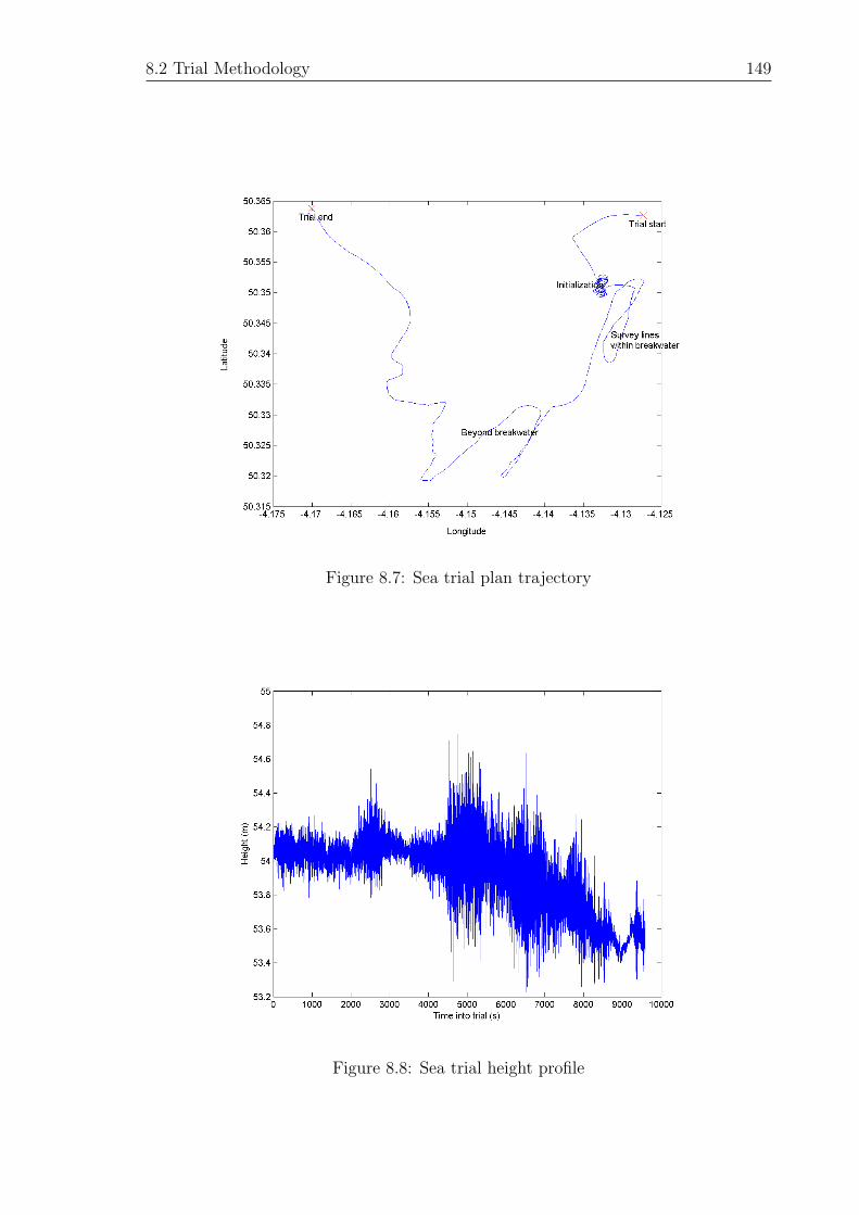
8.2 Trial Methodology 149
Figure 8.7: Sea trial plan trajectory
Figure 8.8: Sea trial height profile

8.2 Trial Methodology 150
Action Time Taken Time Into Trial Key to fig 8.11Steam into Plymouth Sound 1000 s 0-1000 s 1Initialization turns 1000 s 1000-2000 s 2Survey lines within breakwater 1500 s 2000-3500 s 3Steam out beyond breakwater 1100 s 3500-4600 s 4Survey Lines beyond breakwater 1500 s 4600-6100 s 5Steam back to alternative berth 3300 s 6100-9400 s 6Stationary at berth 200 s 9400-9600 s 7
Table 8.1: Times for each action conducted during the sea trial
8.2.5 Vessel Reference Point and Lever Arm Separations
The positional reference point for the trial was taken to be the computational centre
of the CIMU below deck. This is the default option when processing within POSPac
and so was the natural choice. This location was also chosen because the POSRS was
to provide reference data for the trial and all other sensors were to be compared to it.
As has been shown in figure 8.3 the HG1700 was located very close to the CIMU
fitted to the same metal plate. The lever arm between the HG1700 and the CIMU
was measured based on their location on the IMU locating plate and knowledge of the
computation centres of each IMU (all lever arm dimensions are expressed in metres):
lHG1700 =
0.095
0.240
0.005
Due to space restrictions the GPS antennas had to be located on the Marco in areas
which were not ideal for the trial. The ideal location for the GPS antennas when in
operation with the TDD heave algorithm is for them to be collocated with the centre
of gravity of the vessel in order to reduce the effects of roll, pitch and heading on the
heave output. This is usually impossible but at the very least the X and Y lever arm
values should be kept to a minimum, which will also keep lever arm effects on the
heave output to a minimum. In the case of the Marco this was not possible and so
the lever arm values for each antenna were
lLeica1 =
−3.250
2.186
−2.707

8.2 Trial Methodology 151
lLeica2 =
−5.250
2.186
−2.707
lOEM4 =
2.336
0.038
−3.548
lU−Blox =
−4.150
2.186
−2.707
where the x-axis ran from the reference point to the bow, the y-axis ran from the
reference point to the starboard side and the z-axis completed the right hand
coordinate system and ran from the reference point down through the bottom of the
vessel.
The lever arm offsets for the OEM4 and Leica 1 antennas were calculated during the
post processing in POSPac; the lever arm offset for the Leica 2 and U-Blox antennas
were calculated through knowledge of their fixed baseline with respect to the Leica 1
antenna when all three were placed on the boom. Each lever arm value was used to
‘move’ the data recorded with a particular sensor to the computational centre of the
CIMU, the positional reference point for the trial. This was done using the attitude
information extracted from the Applanix POSRS.
Lever arm accuracy has an effect on the accuracy of the TDD heave output because
inaccuracies in the lever arm estimate result in incorrect lever arm compensation and
introduce vertical displacement errors into the TDD velocity algorithm. The effect of
lever arm accuracy can be appreciable at the roll and pitch angles experienced on a
hydrographic survey vessel if a lever arm estimate of within 10 cm or better cannot be
provided. During the Plymouth sea trial the Marco experienced roll and pitch angles

8.3 Trial Results 152
of up to 5 degrees during survey lines, which, using a lever arm estimate with a 10
cm error, would equate to a vertical displacement error of approximately 0.9 cm.
In a marketable TDD heave system used on board a hydrographic survey vessel
POSRS attitude would not be available and as a result careful placing of the GPS
antenna would be an important factor. As already explained this would involve
keeping x and y-axis lever arm to a minimum as they have the greatest effect on
the vertical displacement of the antenna due to changes in vessel attitude. When no
accurate estimate of vessel attitude is available this will help keep attitude dependent
errors to a minimum.
8.3 Trial Results
The results of the sea trial are presented in three distinct sections: POSRS SBET
Data, IMU derived heave and TDD heave. The section for SBET heave looks at the
reference heave data across the entire trial and describes the vertical motion of the
vessel with respect to vessel location and actions. The IMU derived heave section
compares IMU derived heave with SBET heave and assesses its performance in key
areas of the trial. The TDD heave section compares TDD derived heave from the
newly developed algorithm with SBET heave and looks again at the key areas of the
trial.
8.3.1 POSRS SBET Data
The Applanix POSRS was used during the trial to provide reference data against
which the IMU derived heave and the new method of heave measurement using the
low cost U-Blox receiver were compared. This section looks at the quality of the
POSRS SBET data and the derivation of the SBET heave before looking at the
vertical dynamics of the vessel during the entire trial.
8.3.1.1 SBET Data Quality
The SBET data processed in POSPac represented the best available reference trajec-
tory that can be extracted from the data recorded. The reference station data was
provided by the Ordnance Survey and was collected at 1 Hz using a Leica 530 dual

8.3 Trial Results 153
frequency receiver. The raw GPS data collected on the vessel was recorded at 4 Hz
using a Novatel OEM4 dual frequency receiver and the IMU data at 200 Hz using
the Honeywell CIMU. All data were time tagged and logged using the Applanix POS
computer system. The baseline between the reference GPS receiver and the roving
GPS receiver on the vessel ranged between 6 km and 11 km.
The GPS data were processed using the POSGPS software supplied by Applanix.
Reference station and rover data were processed both forwards and backwards to
provide a post processed interferometric GPS solution for the trial. The satellite
availability during the trial can be seen in figure 8.9 and the quality factor for the
post processed GPS solution in figure 8.10. There are five possible quality factors for
processed GPS data within POSGPS:
1. Fixed integer ambiguity
2. Stable float
3. Converging float
4. DGPS or worse
5. Single point
Figure 8.10 shows that much of the processed GPS for the sea trial had a fixed
integer solution with the quality only dropping to a stable float solution for brief
periods during the trial. The post processed GPS solution was then processed with
the raw CIMU data to attain the SBET solution in POSPac.
The post processed Kalman filtered GPS-aided INS solution that has been forward
and backward smoothed within POSPac provides the best estimate of the trajectory
of the vessel during the trial. The POSPac derived estimates of position quality for
the SBET solution were
• North position error (1σ) 1.0 cm
• East position error (1σ) 1.0 cm

8.3 Trial Results 154
Figure 8.9: The number of GPS satellites available during the sea trial
Figure 8.10: The POSGPS quality factor of the processed GPS solution for the seatrial

8.3 Trial Results 155
• Down position error (1σ) 2.3 cm
8.3.1.2 SBET Heave
SBET heave is a data series similar to heave but produced from POSRS post processed
height data. To achieve this data series the SBET height data seen in figure 8.8 were
resampled to 1 Hz and passed through the heave filter described in §6.3.
Figure 8.11 shows the SBET heave data for the entire trial with the plot split into
sections which correspond to the actions represented in table 8.1. This representation
of the heave data is instructive as it clearly shows how heave motion can change
dependent on such factors as sea state and vessel heading. Sections 1-4 of figure 8.11
represent actions undertaken within the breakwater and much of sections 5 and 6
took place beyond the breakwater. Comparison of the heave in these sections shows
the change in sea state once the vessel was beyond the breakwater with a greater
amplitude of heave.
Figure 8.12 and 8.13 show an enlarged view of sections 3 and 5 of figure 8.11
respectively. They show a clear difference in the heave motion of the vessel dependent
on vessel heading and wave direction. In figure 8.12 the first simulated survey line
(2000-2750 s) was in a South-South Westerly direction into the oncoming waves. As
a result of this the amplitude of the measured heave is greater than that during the
second line (2750-3500 s), which was in the opposite direction, the same direction as
wave motion. The same analysis can be applied to the plot shown in figure 8.13. Pitch
motion of the vessel will have had a significant influence on this heave measurement
because of the lever arm due to the CIMU of the POSRS system not being placed at
the centre of gravity of the vessel. This would be mitigated were the data to be used
in a survey but for the purposes of the trial the position of the CIMU is used as the
reference point.
Analysis of the performance of IMU derived heave and the TDD heave algorithm
will be primarily concerned with sections 2, 3 and 5 of the trial as shown in figure
8.11 as these provide dynamics that allow a thorough analysis of inertial based heave
and low cost TDD heave.

8.3 Trial Results 156
Figure 8.11: SBET heave over the complete trial
Figure 8.12: SBET heave data for the two survey lines within the breakwater (section3 of figure 8.11)

8.3 Trial Results 157
Figure 8.13: SBET heave data for the two survey lines outside the breakwater (section5 of figure 8.11)
8.3.2 IMU Derived Heave
The IMU derived heave data was processed using the algorithm laid out in chapter 5
and data collected using a Honeywell HG1700 tactical grade IMU, the manufacturer
published accuracies of which can be viewed in table 2.1.
Figures 8.14, 8.15 and 8.16 show a comparison between SBET heave and IMU
derived heave in three key areas of the trial. Figure 8.14 shows the period of the trial
during which the figure of eight initialization turns were conducted and very clearly
demonstrates the instability of the feedback damping loop applied to the vertical
channel of the IMU output. Vessel turns induce a large input into the heave filter
and the transient performance of the feedback damping loop discussed in chapter 5
results in a ringing of the output. A period of time is required after a turn before the
output from the feedback damping loop has settled once again. This phenomenon
is well known and is seen in figure 8.15 at approximately 2,750 s and in 8.16 at
approximately 5,500 s when the vessel put in a turn between the simulated survey
lines. Comparison of heave error in figures 8.15 and 8.16 with heading data taken from
the SBET solution shows a direct correlation between the IMU derived heave error
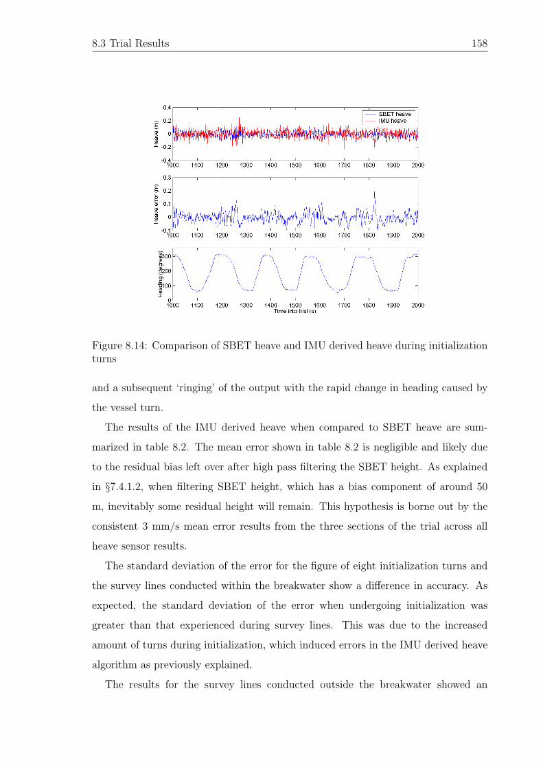
8.3 Trial Results 158
Figure 8.14: Comparison of SBET heave and IMU derived heave during initializationturns
and a subsequent ‘ringing’ of the output with the rapid change in heading caused by
the vessel turn.
The results of the IMU derived heave when compared to SBET heave are sum-
marized in table 8.2. The mean error shown in table 8.2 is negligible and likely due
to the residual bias left over after high pass filtering the SBET height. As explained
in §7.4.1.2, when filtering SBET height, which has a bias component of around 50
m, inevitably some residual height will remain. This hypothesis is borne out by the
consistent 3 mm/s mean error results from the three sections of the trial across all
heave sensor results.
The standard deviation of the error for the figure of eight initialization turns and
the survey lines conducted within the breakwater show a difference in accuracy. As
expected, the standard deviation of the error when undergoing initialization was
greater than that experienced during survey lines. This was due to the increased
amount of turns during initialization, which induced errors in the IMU derived heave
algorithm as previously explained.
The results for the survey lines conducted outside the breakwater showed an

8.3 Trial Results 159
Figure 8.15: Comparison of SBET heave and IMU derived heave during survey lineswithin the breakwater
Figure 8.16: Comparison of SBET heave and IMU derived heave during survey linesoutside of the breakwater

8.3 Trial Results 160
Action Key to figure 8.11 Standard Dev. (1σ) Mean Error(cm) (cm)
Initialization 2 3.8 -0.3Lines within breakwater 3 2.9 -0.3Lines beyond breakwater 5 7.2 -0.3
Table 8.2: IMU derived heave errors
unexpectedly high standard deviation when compared to SBET heave. This was
probably caused by the increased magnitude of heave once outside the breakwater,
which went from a nominal height of ±0.2 m to a value of around ±0.5 m. This
increase in heave magnitude was likely to have an adverse effect on IMU derived
heave output due to the transient response of the feedback damping loop discussed
in chapter 5. The results of IMU derived heave outside the breakwater were a little
disappointing but it should be remembered that the IMU heave algorithm developed
during this thesis is by no means complete and was only ever intended to demonstrate
inertial heave characteristics and give an indication of the likely heave errors. It is
expected that heave measurement using a commercially available inertial based heave
sensor would have greater accuracy.
The IMU derived heave results demonstrated the ability of the inertial based heave
algorithm to measure vessel heave motion, but also highlighted the instability inherent
in the use of that type of algorithm.
8.3.3 TDD Heave
The TDD heave results were achieved using the same three GPS receivers used in
the simulator trial. Raw data were collected on each receiver throughout the trial
and processed using the TDD heave algorithm described in chapter 6. All GPS data
processed were subjected to an elevation mask of 15 degrees.
Each of the data sets collected with the various GPS receivers is discussed in the
following section and the results of the TDD processed heave assessed against SBET
heave. The same three areas of the trial were analysed for TDD heave as were analysed
with the output from the inertial heave algorithm.

8.3 Trial Results 161
8.3.3.1 Leica 530 Receiver
The data collected with the Leica 530 receiver were dual frequency data recorded at
1 Hz. The number of satellites available across the duration of the trial can be seen
in figure 8.17.
Figures 8.18 and 8.19 and 8.20 show the comparison of TDD heave from the Leica
receiver with the SBET derived heave in the three areas analysed in section 8.3.2.
The results are summarized in table 8.3. Taking the over arching view of the results
shown in table 8.3 the level of noise on the TDD heave produced with the Leica 530
receiver can be said to be slightly greater than that found when using the inertial
based heave sensor with standard deviations of the error signal over a centimetre
greater when conducting survey lines. Looking at each area in more detail does show
some interesting results, however.
During the initialization turns undertaken at the start of the trial the error from
the TDD Leica heave showed none of the large heading dependent excursions from
SBET heave that were seen with the IMU derived heave. Indeed, the amount of error
seen in the TDD Leica heave during this period was the same as that seen during the
survey lines. This demonstrated the increased stability of the TDD heave algorithm
over the inertial based algorithm. This was demonstrated again when the vessel turn
between survey lines was undertaken in figure 8.19 (2,750 s). Here no deviation from
the SBET heave was seen as a result of the turn. The magnitude of the standard
deviation of the error for the Leica TDD heave output was of a similar order to that
seen when using IMU derived heave in both of the key areas of the trial, certainly to
within the 2.3 cm POSPac quoted vertical position accuracy of the SBET data. The
main difference between the two sets of results was that the Leica TDD heave was not
adversely affected by vessel turns and instability as was the case in the IMU derived
heave.
The results for the Leica, Novatel and U-Blox TDD heave error during the sur-
vey lines conducted beyond the breakwater are discussed later in this chapter at
§8.3.4along with further analysis relating to the quality of the results.

8.3 Trial Results 162
Figure 8.17: Satellite availability for Leica 530 receiver during sea trial
Figure 8.18: Leica 530 TDD heave error during initialization turns
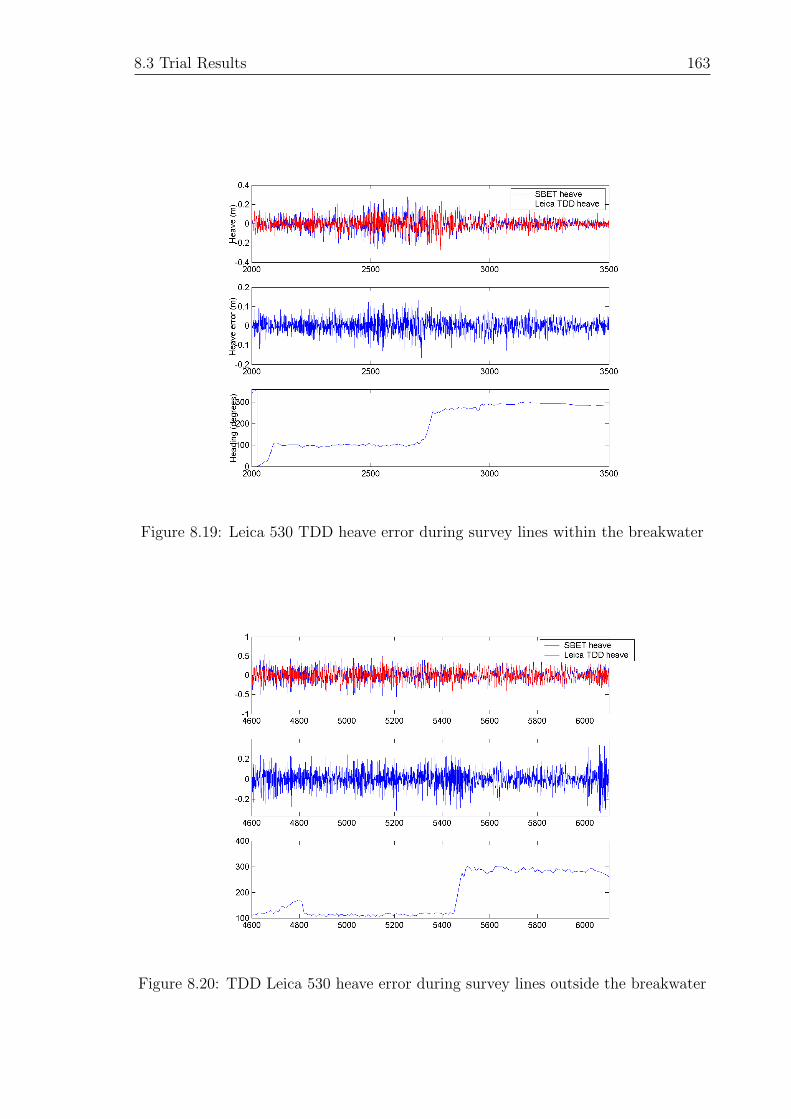
8.3 Trial Results 163
Figure 8.19: Leica 530 TDD heave error during survey lines within the breakwater
Figure 8.20: TDD Leica 530 heave error during survey lines outside the breakwater
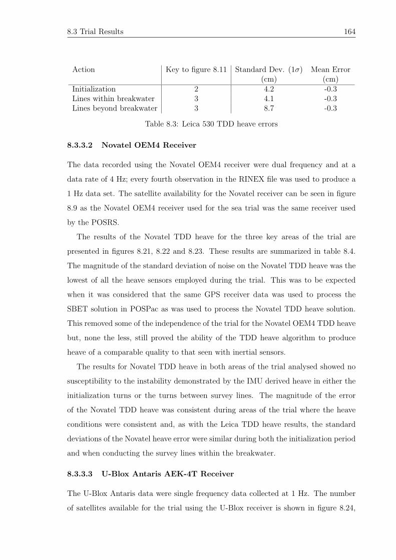
8.3 Trial Results 164
Action Key to figure 8.11 Standard Dev. (1σ) Mean Error(cm) (cm)
Initialization 2 4.2 -0.3Lines within breakwater 3 4.1 -0.3Lines beyond breakwater 3 8.7 -0.3
Table 8.3: Leica 530 TDD heave errors
8.3.3.2 Novatel OEM4 Receiver
The data recorded using the Novatel OEM4 receiver were dual frequency and at a
data rate of 4 Hz; every fourth observation in the RINEX file was used to produce a
1 Hz data set. The satellite availability for the Novatel receiver can be seen in figure
8.9 as the Novatel OEM4 receiver used for the sea trial was the same receiver used
by the POSRS.
The results of the Novatel TDD heave for the three key areas of the trial are
presented in figures 8.21, 8.22 and 8.23. These results are summarized in table 8.4.
The magnitude of the standard deviation of noise on the Novatel TDD heave was the
lowest of all the heave sensors employed during the trial. This was to be expected
when it was considered that the same GPS receiver data was used to process the
SBET solution in POSPac as was used to process the Novatel TDD heave solution.
This removed some of the independence of the trial for the Novatel OEM4 TDD heave
but, none the less, still proved the ability of the TDD heave algorithm to produce
heave of a comparable quality to that seen with inertial sensors.
The results for Novatel TDD heave in both areas of the trial analysed showed no
susceptibility to the instability demonstrated by the IMU derived heave in either the
initialization turns or the turns between survey lines. The magnitude of the error
of the Novatel TDD heave was consistent during areas of the trial where the heave
conditions were consistent and, as with the Leica TDD heave results, the standard
deviations of the Novatel heave error were similar during both the initialization period
and when conducting the survey lines within the breakwater.
8.3.3.3 U-Blox Antaris AEK-4T Receiver
The U-Blox Antaris data were single frequency data collected at 1 Hz. The number
of satellites available for the trial using the U-Blox receiver is shown in figure 8.24,

8.3 Trial Results 165
Figure 8.21: Novatel OEM4 TDD heave error during initialization turns
Figure 8.22: Novatel OEM4 TDD heave error during survey lines within the break-water

8.3 Trial Results 166
Figure 8.23: Novatel OEM4 TDD heave error during survey lines outside thebreakwater
Action Key to figure 8.11 Standard Dev. (1σ) Mean Error(cm) (cm)
Initialization 2 2.5 -0.3Lines within breakwater 3 2.8 -0.3Lines beyond breakwater 5 6.0 -0.3
Table 8.4: Novatel OEM4 TDD heave errors
which shows a depleted number when compared to the satellites available for both
the Leica 530 and the Novatel OEM4. This was caused by the cycle slip handling
algorithm, which removed the observations from satellites in which a slip had occurred
and so reduced the number of usable observations. More complete cycle slip handling
algorithms may be able to not only detect cycle slips but also repair them and allow
data that includes slips to still be used in the TDD processing.
The results for U-Blox TDD heave gained during the sea trial can be seen in figures
8.25, 8.26 and and are summarized in table 8.5.
It can be seen from the plots shown in figure 8.25 that some large excursions of U-
Blox TDD heave from SBET heave occurred during the initialization turns conducted
during the trial (1,050 s, 1,250 s and 1,430 s). These were caused by cycle slips that

8.3 Trial Results 167
Figure 8.24: Satellite availability for U-Blox Antaris during sea trial
Action Key to figure 8.11 Standard Dev. (1σ) Mean Error(cm) (cm)
Initialization 2 5.5 -0.3Lines within breakwater 3 5.1 -0.3Lines beyond breakwater 5 10.2 -0.3
Table 8.5: U-Blox Antaris TDD heave errors
were not detected by the cycle slip handling algorithm developed in this research and
integrated into the TDD heave algorithm. Despite the removal of the vast majority of
the cycle slips in the U-Blox data some still remained and caused spikes in the TDD
velocity estimate, which, when integrated and filtered in the TDD heave algorithm,
produced long periods of heave estimation with large errors. It is thought that further
research into a more suitable cycle slip handling algorithm would remove the remaining
cycle slips resulting in better quality data.
The areas of the heave error plots in figures 8.25, 8.26 and 8.27 that were not
affected by cycle slip based errors were taken to be representative of the magnitude of
errors that would be achievable if all cycle slips were removed from the U-Blox data.
As such, the standard deviation of error values quoted in table 8.5 have had the large
errors caused by undetected cycle slips removed.

8.3 Trial Results 168
Figure 8.25: U-Blox Antaris TDD heave error during initialization turns
Figure 8.26: U-Blox Antaris TDD heave error during survey lines within thebreakwater

8.3 Trial Results 169
Figure 8.27: U-Blox Antaris TDD heave error during survey lines conducted outsidethe breakwater
The magnitude of the standard deviation of heave error for U-Blox TDD heave was
only slightly greater than that seen for Leica TDD heave and heave from the inertial
algorithm. The comparison with Novatel TDD heave showed less favourable results
but this was due to the lack of independence already discussed in §8.3.3.2.
There are no obvious effects on U-Blox TDD heave during the sea trial of the errors
correlated with acceleration seen in chapter 7. This is explained by the plot of the
magnitude of vessel acceleration experienced during the sea trial shown in figure 8.28
which shows that the accelerations experienced during the sea trial were rarely over 2
cm/s2, which, based on the results of the simulator trial, was insufficient to produce
large errors in the U-Blox TDD velocity estimate.
The extra noise in the results from U-Blox TDD heave were expected based on the
assessment of receiver induced measurement noise given in §3.3.4 but did not degrade
the heave solution to the extent where it could not provide heave compensation
capable of meeting the IHO survey order one as described in §4.5. Inertial based
heave sensors also provide heave data to within IHO survey order one (Parker and
Mallace, 2006) meaning that heave measured using the TDD heave algorithm and a

8.3 Trial Results 170
Figure 8.28: Magnitude of acceleration experienced during the plymouth sea trial
U-Blox low cost commercially available receiver is of a comparable standard to inertial
based heave technologies.
8.3.4 The Effect of GPS Data Rate on the Sea Trial Results
The TDD heave results presented in the preceding sections of this chapter were all
based on GPS data recorded at 1 Hz. When the sea trial was originally conducted
it was thought that a 1 Hz data rate would be sufficient to record all the significant
heave motion of the vessel. In reality, the results of the TDD heave during the sea
trial were disappointing, which prompted an analysis of the effects of the 1 Hz GPS
data rate on the resulting TDD heave error.
8.3.4.1 Frequency Range of SBET Heave and 1 Hz TDD Heave Error
Frequency analysis of the SBET heave motion of the vessel during the trial revealed
that there was a significant amount of power in vessel heave motion that occurred
at or above the Nyquist frequency when using data recorded at 1 Hz. Figure 8.29
shows the vessel heave motion across the entire trial in the frequency domain and a
significant proportion of the signal power appears at or above the Nyquist frequency

8.3 Trial Results 171
Figure 8.29: Frequency analysis of SBET heave across the entire trial
of 0.5 Hz. Further frequency analysis was conducted on the SBET heave in sections
relating to each individual survey line conducted within the breakwater. Figures 8.30
(a) and (b) show the heave motion during survey line one (2,000-2,750 s) and survey
line two (2,750-3,500 s) respectively. They show that the heave motion during line
two had significantly less power above or near the Nyquist frequency.
Table 8.6 shows the heave error seen on Novatel OEM4 1 Hz TDD heave during the
survey lines within the breakwater split into the individual lines one and two. When
the plots shown in figure 8.30 were correlated with the data presented in table 8.6 it
was seen that the heave error was greater when the frequencies of the heave motion
were at or above the Nyquist frequency. The same analysis could be conducted on
each individual survey line conducted beyond the breakwater.
Action Standard Dev. (1σ) Mean Error(cm) (cm)
Survey line 1 4.0 -0.3Survey line 2 1.8 -0.3
Table 8.6: Novatel OEM4 1 Hz TDD heave error during lines conducted within thebreakwater
It was thought that the heave experienced by the vessel that exceeded or was in

8.3 Trial Results 172
Figure 8.30: Frequency analysis of SBET heave during line 1 (a) and line 2 (b)conducted within the breakwater
the proximity of the Nyquist frequency caused the 1 Hz heave motion to be under
sampled. This resulted in signal aliasing in the heave motion when expressed at 1 Hz.
8.3.4.2 Novatel OEM4 4 Hz TDD Heave
The findings resulting from the heave frequency analysis were endorsed by the results
gained from Novatel TDD heave when processed at 4 Hz shown in figures 8.31, 8.32
and 8.33 for the three key areas of the trial, results which are summarized in table
8.7. The Novatel OEM4 receiver was the only receiver to record data at a higher rate
during the sea trial and so was the only receiver for which higher rate TDD heave
could be processed.
Action Key to figure 8.11 Standard Dev. (1σ) Mean Error(cm) (cm)
Initialization 2 1.6 -0.3Lines within breakwater 3 1.7 -0.3Lines beyond breakwater 5 2.7 -0.3
Table 8.7: Novatel OEM4 4 Hz TDD heave errors
The results for the 4 Hz Novatel OEM4 data presented in table 8.7 showed a marked

8.3 Trial Results 173
Figure 8.31: Novatel OEM4 4 Hz TDD heave error during initialization turns
improvement over the results for the same receiver recorded at 1 Hz and shown in
table 8.4. The increased data rate pushed the Nyquist frequency up to 2 Hz, which
was more than adequate to cover all the frequencies of motion seen in figure 8.29
so the 4 Hz heave was not subject to the aliasing which occurred in the 1 Hz data.
In addition, the heave error shown in figures 8.32 and 8.33 can be seen to be of a
similar magnitude during both individual lines leading to the conclusion that higher
frequency heave motion was no longer adversely affecting the heave error.
Doubts were expressed in §8.3.3.2 as to the independence of Novatel OEM4 TDD
heave from the SBET reference data given that the same GPS data being used for
both heave solutions. For this reason a new SBET solution was processed using the
CIMU data aided by 1 Hz Leica 530 GPS data. A heave estimate based on this new
SBET solution was compared to the Novatel 4 Hz TDD heave estimate and the results
are presented in table 8.8. These results show similar levels of accuracy to those seen
in table 8.7 and demonstrate the high quality of heave estimation possible using the
TDD heave algorithm.

8.4 Plymouth Sea Trial Summary 174
Figure 8.32: Novatel OEM4 TDD 4 Hz heave error during survey lines conductedwithin the breakwater
Action Key to figure 8.11 Standard Dev. (1σ) Mean Error(cm) (cm)
Initialization 2 1.5 0.4Lines within breakwater 3 1.8 0.4Lines beyond breakwater 5 2.7 0.4
Table 8.8: Novatel OEM4 4 Hz TDD heave errors when compared to SBET dataprocessed using 1 Hz Leica 530 GPS data
8.4 Plymouth Sea Trial Summary
The sea trial was conducted on 2 August 2006 between 09:30 and 12:30 in and around
the Plymouth Sound. Data was collected using three GPS receivers of various grades
to produce TDD heave, an HG1700 IMU to create IMU derived heave using the
algorithm developed during this project and a GPS-aided INS Applanix POSRS to
provide truth data.
The trial has successfully proved the ability of the TDD heave algorithm to estimate
heave to within the tolerances required to achieve the IHO survey order 1, while
removing the troubling issues surrounding inertial based heave algorithms such as
stability and usability. This section summarizes the main results of the sea trial.

8.4 Plymouth Sea Trial Summary 175
Figure 8.33: Novatel OEM4 TDD 4 Hz heave error during survey lines conductedbeyond the breakwater
8.4.1 IMU Derived Heave
IMU derived heave using the inertial heave algorithm developed during this project
was compared to SBET heave recorded using the highly accurate GPS-aided INS
Applanix POSRS. The results have shown that the IMU derived heave had an error
standard deviation of 3.8 cm during the period of figure of eight initialization turns,
2.9 cm during the simulated survey lines conducted within the breakwater and 7.2 cm
during the simulated survey lines conducted outside the breakwater. The magnitude
of the errors in IMU derived heave were somewhat disappointing but they should be
taken in the context of the IMU heave algorithm quality. The purpose of the IMU
heave algorithm is to give an idea of the accuracies possible with inertial technologies
but also to highlight their shortcomings in respect to instability and usability.
The instability problems associated with the use of inertial technologies in this
application were highlighted with deviations of IMU derived heave from SBET heave
during and after turns, a phenomenon known as turn induced heave that resulted in
decreased accuracy. Usability is always an issue with inertial based heave measure-
ment as the time constant and damping coefficients for the feedback loop must be

8.4 Plymouth Sea Trial Summary 176
optimally set.
8.4.2 TDD Heave
The TDD heave produced from the two high grade GPS receivers used in the trial
was of a similar accuracy to that seen when using inertial sensors with the Leica
receiver achieving error standard deviations of 4.2 cm during initialization, 4.1 cm
during the survey lines within the breakwater and 8.7 cm during survey lines beyond
the breakwater. The Novatel results were similar, achieving 2.5 cm, 2.8 cm and
6.0 cm in the same periods of the trial. The results were not just concerned with
heave measurement accuracy, however, and it was important to note that the TDD
heave algorithm exhibited no turn induced heave, which corrupted the accuracy of
the inertial based heave during the initialization period and during the turn after the
first survey line. The TDD heave algorithm also places no burden on the user to set
the filter parameters to suit vessel characteristics and current sea state conditions.
The results of the U-Blox TDD heave, although slightly degraded in accuracy from
the results seen from the two higher grade receivers and the IMU derived heave,
showed that the new TDD heave algorithm designed for use with low cost GPS
receivers is likely to be able to compete with inertial based algorithms to provide
heave data capable of IHO survey order one. The main problem with data from
the U-Blox receiver compared to the data from the higher grade receivers was the
existence of a large number of cycle slips, some of which were not detectable using the
algorithms employed in this research. Still the standard deviations of the heave error
using U-Blox TDD heave were 5.5 cm, 5.1 cm and 10.2 cm in the three key areas of
the trial.
A key factor in the accuracy of the TDD heave estimates quoted above has been the
data rate of the GPS data. All the results were based on 1 Hz GPS data and analysis
has shown that this was insufficient to capture all the heave motion experienced by
the vessel and prevent aliasing in the heave estimation. Using Novatel OEM4 data
collected at 4 Hz has demonstrated much improved accuracies (1σ) of 1.5 cm, 1.8 cm
and 2.7 cm during the three key areas of the trial when compared to an independent
SBET solution processed using 1 Hz Leica 530 GPS data.

8.4 Plymouth Sea Trial Summary 177
It is strongly expected that U-Blox GPS data recorded at 4 Hz would see accuracy
improvements over its 1 Hz counterpart of a similar order to those seen when using
the Novatel OEM4.

Chapter 9
Summary, Conclusions and FutureRecommendations
This chapter of the thesis summarizes the work undertaken for the project highlighting
the main points and the areas of novelty that the work has accomplished. There is
also a section that draws conclusions from the results found during the two sets of
trials conducted. Finally, there is a section that makes some recommendations for
future work based on the experience gained throughout the project and the results of
the two trials.
9.1 Thesis Summary
The aim of the project was to develop a heave algorithm for use with off the shelf
low cost GPS receivers such as the U-Blox Antaris. This algorithm was to overcome
some of the problems and limitations associated with the use of inertial sensors for
the measurement of heave in three areas:
• Cost
• Stability
• Usability
This has been achieved through the development of a highly accurate velocity
estimation algorithm using stand-alone low cost GPS receivers, termed temporal
double difference (TDD). Carrier phase pseudo-range observations from adjacent
epochs were differenced to produce user velocity, the vertical channel of which was
178

9.1 Thesis Summary 179
then integrated to produce relative vertical position. A high pass filter was also
designed that was then used to remove any drift on the relative position output that
may exist due to bias errors on the vertical velocity estimation, resulting in highly
accurate heave estimation.
The algorithm has been extensively tested in both a simulated and a real world
marine environment. The simulator trial, conducted using a Spirent hardware sim-
ulator, tested the accuracy of the TDD velocity algorithm under varying dynamic
conditions and using receivers of varying grades allowing the errors associated with
low cost receivers to be quantified. The sea trial was conducted using a vessel owned by
Sonardyne International Ltd. and allowed the testing of the algorithm under marine
conditions. The TDD heave algorithm was implemented using data collected from
varying grades of GPS receiver and tested against the results from both an inertial
heave algorithm developed for the project and highly accurate truth data recorded
using an Applanix POSRS GPS-aided INS system.
The recent introduction of off the shelf low cost GPS receivers with the ability to
measure and record the raw carrier phase pseudo-range observable has allowed their
use in the TDD algorithm developed for this project, and it has been the first work
to look at their use for the measurement of hydrographic survey vessel heave motion.
The simulator trial conducted using the Spirent simulator purchased by the IESSG
has, for the first time, quantified the errors associated with low cost receivers in the
measurement of the carrier phase pseudo-range observable through the comparison of
the U-Blox Antaris results with those from higher grade dual frequency receivers, and
through the collection of data under varying dynamic scenarios. The comprehensive
nature of the sea trials conducted in Plymouth have been the first to have produced a
full assessment of the TDD heave algorithm implemented on commercially available
low cost receivers. It has tested the algorithm against an entire suite of further
heave motion sensors including the use of various stand-alone GPS receivers for TDD
heave, an inertial based heave sensor and heave data collected using the POSRS; this
is something that is not seen in previous works.
9.2 Conclusions 180
9.2 Conclusions
Two separate trials have been conducted for this thesis, which have been used to
thoroughly test different aspects of the TDD algorithm developed during the project.
Both of these trials have proven the performance of the TDD velocity and heave
algorithms and the conclusions that can be drawn from each are presented below.
9.2.1 The Spirent Simulator Trials
The Spirent simulator trial conducted as part of the research contained within this
thesis has been the first to explore the quality of the recorded carrier phase pseudo-
range observable measured with commercially available low cost GPS receivers when
compared to the measurements taken from dual frequency receivers. By using three
separate receivers of varying grades to record simulated data from the same scenarios
receiver based errors were isolated and quantified. This was extended to cover data
from three distinct sets of dynamics that were able to test the performance of the
receiver signal tracking loops under dynamic stress. Further tests were able to intro-
duce simulated errors such as tropospheric and ionospheric delay allowing their effects
on the TDD velocity estimation to be determined. The conclusions drawn from the
Spirent simulator are itemized below.
• Under static conditions the TDD velocity estimation using the U-Blox receiver
was of a comparable quality to those seen when using the Novatel and Leica
receivers. This is thought to be caused by the limitation of the bandwidth
of the signal tracking loop within the U-Blox receiver based on the knowledge
that the receiver is stationary. The use of this extra information enables the
U-Blox receiver to level the playing field somewhat, allowing the signal tracking
loops within the receiver to record accurate measurements of the carrier phase
pseudo-range observable with reduced tracking loop bandwidth whilst acting
well within their dynamic stress limitations.
• When under dynamic conditions, of the order of which may be expected in
a marine environment, a divergence in the performance of the three receivers
was found to exist. The quality of the measurements recorded with the U-Blox

9.2 Conclusions 181
receiver was now significantly reduced when compared to those recorded using
either the Novatel or the Leica. As such the TDD heave estimates produced
using the data from the U-Blox receiver were also less accurate than those
produced from data recorded using the Leica or Novatel receivers. Errors in
TDD heave from the U-Blox receiver were approximately an order of magnitude
greater than those seen from the other receivers at the highest frequencies of
motion. These results were emphatically endorsed by those seen when the
receivers were subjected to a high dynamic scenario.
• The velocity estimate calculated using the TDD velocity algorithm can be
significantly affected by the rate of change of the errors associated with the
atmosphere. This was proven during trials two and three when tropospheric
and ionospheric errors were modeled within the simulator. The magnitude
of potential error in TDD velocity if the simulated tropospheric error source
was left unmitigated was ±2 mm/s in horizontal velocity and ±4 mm/s in
vertical velocity. The magnitude of possible error experienced for unmitigated
ionospheric delay was smaller at ±1 mm/s in horizontal velocity and ±1.5 mm/s
in vertical velocity suggesting that the penalty in TDD velocity accuracy for
single frequency data collection may be small.
• The final simulator trial brought together all the aspects of the previous trials
by testing the full TDD velocity and heave algorithms in the static and marine
environments with atmospheric errors simulated. This provided a natural last
step between the simulator trial and the collection of real data and the results
were similar to those seen in trial one, which was to be expected given the results
that of the previous trials.
• As a final prelude to the collection of data for the sea trial real static GPS
data were collected using each of the three receivers used in the simulator trial
along with their respective antennas. The results of this trial endorsed the
results of the simulator trial inasmuch as the TDD velocity performance of the
U-Blox receiver was equal to that of the Leica an Novatel receivers under static
conditions.

9.2 Conclusions 182
9.2.2 The Sea Trial
The sea trial was conducted in order to test the TDD heave algorithm calculated using
data recorded with the three receivers previously used in the simulator trial against
an IMU derived heave estimate and highly accurate Applanix POSRS reference data.
The magnitude of the IMU derived heave error was considered to be too great,
which was likely due to the quality of the algorithm in use. The heave algorithm
developed during the project was simply a damped INS vertical channel and employed
none of the velocity aiding algorithms that commercial heave sensors use, which are
explained in §2.5. The IMU derived heave results did demonstrate the stability and
usability issues implicit with the use of inertial heave sensors, however.
The TDD heave for each receiver used in the trial was compared to the SBET
heave solution. The results demonstrated clearly the benefits available to the TDD
heave user compared to the inertial based heave user. Each receiver’s TDD heave
output demonstrated increased stability over IMU derived heave and no tuning was
required by the user as is required with inertial heave sensors. The magnitude of the
errors seen in the TDD heave solution using all three receivers were larger than was
expected due to the under sampling of vessel heave motion at 1 Hz. Even with the
aliasing that occurred due to that under sampling, the results do show the ability
of U-Blox TDD heave to compete with heave produced from other GPS receivers in
terms of accuracy.
The TDD heave results for the sea trial were all based on GPS data recorded at 1
Hz. Through analysis this data rate was found to be inadequate for the measurement
of the frequency of heave motion experienced by the vessel during the trial. A 4
Hz TDD heave solution was processed using data collected from the Novatel OEM4
receiver, the only receiver used in the trial to log raw observables at a higher data
rate. The Novatel 4 Hz TDD heave was compared to an SBET solution that was
processed in POSPac using the 1 Hz Leica 530 collected during the trial; this was
done so as to provide independent reference data as the previous SBET solution was
processed using the Novatel OEM4 data. The Novatel 4 Hz TDD heave showed a
vastly increased level of performance over the heave solutions using 1 Hz data and

9.3 Recommendations for Future Work 183
exhibited no adverse effects due to higher frequency heave motion.
Overall, the results of the sea trial show the ability of TDD heave to measure heave
to the accuracy required for at least IHO survey order one and possibly IHO special
order when using high grade GPS receivers such as the Novatel OEM4. It is expected
that U-Blox TDD heave would see a marked improvement in accuracy over the figures
stated in chapter 8 if data were collected at a higher rate, say 4 Hz. The TDD heave
outputs exhibited no errors due to the temporal instability that is experienced in the
use of inertial based heave sensors and also required no inputs from the user. These
factors show the ability of TDD heave using commercially available low cost GPS
receivers to compete with inertial based sensors in terms of accuracy, and generate
savings to the survey industry. These savings come in the form of reduced unit cost,
reduced lead in time to survey lines and reduced user burden.
9.3 Recommendations for Future Work
The research conducted during this project and presented in this thesis has proven the
ability of commercially available low cost GPS receivers to be used in a TDD heave
algorithm that can potentially measure heave to meet IHO survey order one. It has
also highlighted some of the limitations of these receivers under high accelerations and
quantified the level of error introduced by them compared to higher grade receivers.
In order to continue the research and make further advancements in this field certain
recommendations are made here for future work.
The first, and most obvious, recommendation to be made is that a further sea
trial is carried out using the U-Blox GPS receiver or similar recording data at a rate
suitable to adequately sample the entire frequency spectrum of vessel heave. the work
carried out in this thesis proves the TDD algorithm using a Novatel OEM4 receiver
and suggests that similar results could be achievable using a U-Blox receiver but a
sea trial is required to fully prove that.
A further recommendation surrounds the issue of vessel attitude. Many applica-
tions for heave sensors require the estimation of vessel attitude such as the need for
echo-sounder beam steering onboard a hydrographic survey vessel. This is provided as

9.3 Recommendations for Future Work 184
an output when using inertial based AHRS units but is not available through the use of
a single receiver in a TDD heave algorithm. The use of multiple receivers may provide
a way to resolve attitude rate through their relative TDD velocities, however, and this
should be explored fully so that TDD heave sensors may compete with inertial based
technologies in the hydrographic survey industry market. In many instances multiple
receivers already exist onboard vessels and the exploitation of raw measurements from
these may remove the need the installation of others; a microprocessor based system
that can exploit these opportunistic GPS observables to produce heave and attitude
rate may be possible.
A severe limitation of the U-Blox receiver used in this trial to produce reliable
heave measurement has been the requirement of a robust and accurate cycle slip
detection and repair algorithm. The algorithm developed for use in this thesis is
based on analysis of the least squares residuals from the TDD velocity algorithm and
removing any that appear to differ from the others by a nominal value. This has
proved adequate for the purposes of this project and has removed the majority of
cycle slips but some still remained. Removal or repair of all cycle slips is a necessary
step in the production of a robust low cost TDD heave estimate as the nature of
the TDD heave algorithm exacerbates the effects of cycle slips when they are passed
through the high pass filter.
A final recommendation offered is the coupling of low cost GPS receivers with
low cost MEMS technology IMUs to provide a complete low cost GPS-aided INS for
use in the hydrographic survey market. It is thought that the use of inertial based
algorithms exploited by AHRSs implemented with MEMS grade IMUs could be aided
using the TDD velocities produced from a low cost GPS receiver to produce a Kalman
filtered heave solution that will show robustness to momentary GPS signal loss. This
notion can be extended further to produce a complete GPS-aided INS based solely on
low cost sensors that can provide a low cost alternative to systems currently on the
market such as the Applanix POSMV.

References
Admiralty, 1987. Admiralty Manual of Navigation.
Alkan, R., 2003. Reduction of heave, pitch and roll effects in hydrographic surveying.
Survey Review (37), 208–217.
Ashkenazi, V., Moore, T., Lowe, D., Moore, D., Woodworth, P., Rae, J., 1996.
Offshore sea measurement using GPS. Civil Engineering Surveyor GIS/GPS Sup-
plement .
Bingley, R., 1998. GPS observables and algorithms, lecture presented as part of the
Royal Navy Long Hydrographic Course.
Bisnath, S., Wells, D., Howden, S., Dodd, D., Wiesenburg, D., 2004. Developement
of an operational RTK GPS-equipped buoy for tidal datum determination. Inter-
national Hydrographic review 5 (1), 54–64.
Blanchard, R. L., November 1971. A new algorithm for computing inertial altitude
and vertical velocity. IEEE Transactions on Aerospace and Electronic Systems AES-
7 (6).
Canter, P., Corcoran, R., October 2004 2004. New generation of POS a boost for
hydrographic surveying. International Ocean Systems .
Chamber of Shipping, 2004. Annual review.
Chang, C. C., Sun, Y. D., 2004. Application of a GPS-based method to tidal datum
transfer. The Hydrograghic Journal (112), 15–20.
Collatz, L., 1966. The Numerical Treatment of Differential Equations. Springer.
185

References 186
Collins, J. P., Langley, R. B., March 1999. Possible weighting schemes for GPS
carrier phase observations in the presence of multipath. Tech. Rep. DAAH04-96-C-
0086/TCN98151, United States Army Corps of Engineers Topographic Engineering
Centre.
Corcoran, R., Pronk, B., 2003. POS/MV model 320 V3 ethernet and SCSI ICD.
Farrell, J., Barth, M., 1999. The Global Positioning System and Inertial Navigation.
McGraw-Hill.
Gelb, A., 1982. Applied Optimal Estimation, 7th Edition. MIT Press.
Godhavn, J.-M., September 2000. High quality heave measurements based on GPS
RTK and accelerometer technology. In: Oceans 2000 MT S/IEEE Conference and
Exhibition. Vol. 1. pp. 309–314.
GPS JPO, September 1997. Interface Control Document ICD-GPS-200. GPS Joint
Programs Office, Revision IRN-200C-002.
Grubin, C., 1970. Derivation of the quaternion scheme via the euler axis and angle.
Journal of Spacecraft and Rockets 7, 1261–1263.
Hare, R., September 1995. Depth and positioning error budgets for multi-beam
echosounding. International Hydrographic Review .
Hide, C., 2003. Integration of GPS and low cost INS measurements. Ph.D. thesis,
University of Nottingham.
Hide, C., Blake, S., Meng, X., Roberts, G., Moore, T., Park, D., September 2005. An
investigation in the use of GPS and INS sensors for structural health monitoring.
In: ION GPS 2005. Long Beach, California.
Hide, C., Moore, T., Smith, M., August 2004. Performance of gps and low-cost ins
integration in marine survey. International Hydrographic Review 5 (2).
Hoffmann-Wellenhoff, B., Lichtenegger, H., Collins, J., 2001. GPS: Theory and
Practice, 5th Edition. Springer-Verlag/Wien.

References 187
IEEE, 1979. Programs for Digital Signal Processing. IEEE Press, algorithm 5.1.
IHO, April 1998. IHO standards for hydrographic surveys: Special publicatiion no.
44.
Imahori, G., Gibson, W. M., Tronvig, K., 2003. Improvements to water level reducers
for hydrographic surveys in hydrodynamically complex tidal regimes. In: US Hydro
2003. Mississippi.
Ingham, A. E., 1992. Hydrography for the Surveying Engineer. Blackwell.
Itani, K., Hayashi, N., Ueno, M., 2000. Low-cost wave sensor using time differential
carrier phase observations. In: ION GPS 2000. Salt Lake City.
James, G., 2001. Modern Engineering Mathematics, 3rd Edition. Prentice Hall.
Jeffrey, A., 1989. Mathematics for Engineers and Scientists, 4th Edition. van Nostrand
Reinhold.
Jekeli, C., 2001. Inertial Navigation Systems with Geodetic Applications. de Gruyter.
Kalman, R. E., 1960. A new approach to linear filtering and prediction problems.
Transactions of the ASME–Journal of Basic Engineering 82, 35–45.
Kaplan, E. D., 1996. Understanding GPS: Principles and Applications. Artech House.
Kayton, M., Fried, W. R., 1997. Avionics Navigation Systems, 2nd Edition. John
Wiley & Sons.
Kielland, P., Hagglund, J., 1995. Using DGPS to measure the heave motion of
hydrographic survey vessels. In: Institute of Navigation NTM 95.
Klobuchar, J. A., 1996. Ionospheric Effects on GPS. Vol. 1 of Global positioning Sys-
tem:Theory and Applications. American Institute of Aeronautics and Astronautics,
pp. 485–515.
Kongsberg, January 2005. MRU Z Data Sheet.

References 188
Kreyszig, E., 1988. Advanced Engineering Mathematics, sixth Edition. John Wiley &
Sons.
Kunysz, W., January 1998. Effect of antenna performance on the GPS signal accuracy.
In: ION National Technical Meeting 1998. Long Beach, California.
Langley, R. B., June 1997. GPS receiver system noise. GPS World 8 (6), 40–45.
Lidner, D. K., 1999. Introduction to Signals and Systems. McGraw-Hill.
Luscombe, J., 2003. Gyrocompass velocity aiding, internal report for Sonardyne Intl.
Marine Accidents and Investigations Branch, 2004. Annual report.
Martin, R. J., Broadbent, G. J., 2004. Chart datum for hydrography. The Hydro-
graphic Journal (112), 9–14.
Maybeck, P. S., 1979. Stochastic models, estimation, and control. Vol. 141 of
Mathematics in Science and Engineering.
Misra, P., Enge, P., 2004. Global Positioning System: Signals, Measurement and
Performance. Ganga-Jamuna Press.
Mostafa, M., Hutton, J., Reid, B., 2001. GPS/IMU products - the applanix approach.
In: 48th Photogrammetry Week. Stuttgart.
National Geodetic Survey, March 2007. Continually operating reference stations.
[Online], available at <http:\\www.ngs.noaa.gov/CORS/cors-data.html>.
Parker, D., Mallace, D., 2006. Motion sensor performance: Direct comparison using
2005 common dataset. Hydro International 10 (1).
Parkinson, B. W., Spilker, J. J., 1996a. Global Positioning System: Theory and
Application. Vol. 1. American Institute of Aeronautics and Astronautics.
Parkinson, B. W., Spilker, J. J., 1996b. Global Positioning System: Theory and
Application. Vol. 2. American Institute of Aeronautics and Astronautics.
Port of London Authority, 2004. Port of london authority annual report. Tech. rep.

References 189
Reefer, 2007. Annual reefer shipping market review and forecast.
Reinking, J., Harting, A., October 2002. Heave determination by stand-alone GPS
and/or inertial sensors. In: Hydro 2002. Kiel, Germany.
Riley, J. L., Milbert, D. G., Mader, G. L., 2003. Hydrographic surveying on a tidal
datum with kinematic GPS: NOS case study in delaware bay. In: US Hydro 2003.
Mississippi.
Rogers, R. M., 2000. Applied Mathematics in Integrated Navigation Systems. AIAA.
Ryan, S., Lachapelle, G., E, C. M., September 1997. DGPS kinematic carrier phase
signal simulation analysis in the velocity domain. In: Proceedings of ION GPS ’97.
Kansas City, Missouri.
Sanders, P., 2003. RTK tide basics. Hydro International 7 (10), 26–29.
Scarfe, B., 2002. Measuring water level correction (wlc) using RTK GPS. The
Hydrograghic Journal (104).
Serrano, L., Don, K., Langley, R. B., September 2004a. A single GPS receiver as a real
time, accurate velocity and acceleration sensor. In: ION GNSS 2004. Long Beach,
CA, pp. 2021–2034.
Serrano, L., Donghyun, K., Langley, R. B., Itani, K., Ueno, M., January 2004b. A
GPS velocity sensor: How accurate can it be? - a first look. In: ION NTM 2004.
San Diego, CA.
Siouris, G., 1993. Aerospace Avionic Systems A Modern Synthesis. Academic Press.
Spirent, September 2006. SimGen Software User Manual. Spirent Communications
Ltd., Aspen Way, Paignton, Devon, No. DGP00686AAA, Issue 1-20.
STANAG, 1990. NATO standardization agreement (STANAG) 4294.
Steiler, B., Winter, H., September 1982. Flight test instrumentation volume 15 on
gyroscopic instruments and their application to flight testing. AGARD AG-160-
Vol.15, NATO.

References 190
Terai, K., 2004. Precise vertical position fixing: Kinematic-gps validation in japans
inland seas. Hydro International 9 (10), 7–9.
Titterton, D., Weston, J., 2004. Strapdown Inertial Navigation Technology, 2nd
Edition. IEE.
USDOD, 1991. NAVSTAR GPS user equipment introduction. Tech. rep., GPS Joint
Program Office.
van Dierendonck, A. J., 1996. GPS Receivers. Vol. 1 of Global positioning System:
Theory and Applications. American Institute of Aeronautics and Astronautics,
Ch. 8, pp. 329–407.
van Graas, F., Soloviev, A., 2004. Precise velocity estimation using a stand-alone GPS
receiver. Navigation: Journal of the Institute of Navigation 51 (4).
VTTSS Ltd, 2005. Meridan Attitude and Heading Reference System Data Sheet.
Weiss, I., DeVries, T., October 1977. Ship motion measurement filter design. IEEE
Journal of Oceanic Engineering 2, 325–330.
Welch, G., Bishop, G., February 2001. An introduction to the kalman
filter. Tech. Rep. TR 95-041, University of North Carolina, available
at <http://www.cs.unc.edu/~welch/media/pdf/kalman_intro.pdf>, [Accessed
March 2007].
Zhang, J., Zhang, K., Grenfell, R., Deakin, R., 2006. GPS satellite velocity and
acceleration determination using the broadcast ephemeris. Journal of Navigation
59 (2), 293–305.
Zhoa, J., Hughes Clarke, J. E., Brucker, S., Duffy, G., 2004. On the fly gps tide
measurement along the saint john river. International Hydrographic Review 5 (3),
48–58.