Improved randomized approximation algorithms for lot-sizing …dbertsim/papers/ApproximationAlgorithms/Improved... · Improved Randomized Approximation Algorithms for Lot-Sizing Problems

Improved Randomized Approximation Algorithms for Lot-Sizing Problems

Chung-Piaw Teo 1 Dimitris Bertsimas 1

Sloan School of Management and Operations Research Center, MIT

1 Introduction

We consider in this paper multi-product, lot-sizing problems that arise in man- ufacturing and inventory systems. We describe the problem in a manufactruring setting. There is a set N of products. For each product j E N there is a set ~-j (called predecessors of product j) of products consumed in producing product j. We define the product network G to be a directed network with node set N and arc set A = {(i,j) : i E ~rj). In other words, the network G corresponds to the flow of materials in the system and contains no circuit.

External demand di for product i is assumed to be constant in time. Clearly in order to satisfy the demand orders should be placed for the products dynami- cally in time. If an order is placed for product i, an ordering cost Ki is incurred. Moreover, an incremental echelon holding cost hi is incurred per unit time the item spends in inventory. The production rate is assumed to be infinite. The objective is to schedule orders for each of the products over an infinite horizon so as to minimize long-run average cost.

As the optimal dynamic policy can be very complicated, the research community (see for instance Roundy [18, 19], Jackson, Maxwell and Muckstadt [10], Muckstadt and Roundy [14]) has focused on stationary and nested policies de- fined as follows: Orders are placed periodically in time at equal intervals, for each of the products in the system (stationary policies). If product j precedes product i, then an order is placed for product j only when an order is placed for product i at the same time (nested policies). Therefore, under a stationary and nested policy the objective is to decide the period Ti that an order is placed. The reason stationary and nested policies are attractive is that they are easy to implement. Muckstadt and Roundy [14] discuss in detail the rationale of using order intervals ~ as variables.

The problem of designing an optimal stationary and nested policy can then be formulated (see [18]) as the following nonlinear integer programming problem.

(PNs) = m i n G(T) -= i~eN (~ + Hi~)

~jj e {1,2,3.. .} if (i,j) e A,

360

Ti = kiTL for each i, ki E Z+

Period TL is called the base period and it can be constant or allowed to vary, depending on the model. The coefficient Hi is given by Hi = (hi - ~;-]~je~ hj)Di and Di represents the aggregate demand, which is calculated recursively starting from products with si = g by Di = di + ~k~s~ Dt~ (si is the set of successors of product i).

We consider the following convex relaxation of the problem:

T~ >_ ~ if (i,j) E A, 2q >_ TL for each i.

Notice that the constraints Ti > Tj model the condition that policies are nested. As the objective function is convex, the relaxation (PR) can be solved in

polynomial time using interior point algorithms or the algorithm by Hochbaum and Shanktikumar [9]. For systems with special structure the runnning time can be improved substantially. For instance, ff G is a tree, Jackson and Roundy [11] show that the relaxed problem can be solved in O(nlogn) time, where n -- ]N I, When G corresponds to a star graph, Queyranne [151, and also Lu Lu and Posner [12] showed that the relaxed problem can be solved in O(n) time, using a linear time median finding algorithm.

Regarding approximation algorithms, Roundy ([18, 19]), and Maxwell and Muckstadt [13] showed how to round an optimal solution of the relaxed problem (PR) to a feasible solution for (PJvs). The policies constructed are called power- of-two policies, where each 7~ is of the form 2P~TL, where p~ is integer. Let ZH be the value of the heuristic used. They obtained the following bounds:

1. f f TL is not fixed, but subject to optimization, then

Z / / < 1 ~ 1 . 0 2 .

zR - v~log 2

2 . If TL is fixed, then

- - ~ 1 . 0 6 . z R -

The technique used is deterministic rounding and convex duality. The technique utilizes the properties of the optimal relaxed solution. In both cases the bounds are tight. These results are often referred in the literature as 98% and 94% effective lot-sizing policies respectively.

These results have been extensively studied and extended to other versions of lot-sizing problems: finite production rates (Atkins, Queyranne and Sun [1]),

361

individual capacity bounds of the form 2t~TL < Ti < 2UiTL and more general cost structures (Zheng [21]), and backlog (Atkins et al. [1]). All these extensions use determinisitc rounding to generate power-of-two policies with the same 94% and 98% bounds.

In this paper, we propose a new approach to these lot-sizing problems that uses randomized rounding. This design technique has been used extensively by the discrete optimization community. It was first introduced by Raghavan and Thompson [16], and was used subsequently for a variety of other combinatorial problems. See for instance Goemans and Williamson [7, 8], Bertsimas and Vohra [3], Bertsimas et al. [2]. Our contributions in this paper are as follows:

. We propose new 94% and 98% randomized rounding algorithms for Prob- lem (PNs) under both the fixed and the variable base period models. Our proof is simple and unlike the original deterministic rounding does not depend on the structure of the optimal solution. Roundy's 98% algorithm can be obtained by derandomizing our algorithm. However, derandomizing the 94% algorithm leads to a different deterministic algorithm. The randomized rounding method is interesting in its own right as it introduces dependencies in the rounding process and generates random variables with distributions with nonlinear density functions.

. We study a generalization of the fixed based model by allowing the base period TL to vary over a finite set of choices {2k/PTL : k integer}, with p, TL fixed. We propose a randomized rounding algorithm that produces a

1 power-of two policy with bound ~ ~ +1 , where p denote the number

of points TL is allowed to vary. For p = 1 and p - or, the bound reduces to 1.06 and 1.02 respectively. For the one warehouse, multi-retailer problem (OWMR), Lu Lu and Posner [12] have also obtained a similar bound for a class of integer-ratio policies.

3. For a general production distribution network under nested policies, we propose new convex relaxations and randomized rounding algorithms that use ~ = 2P~TL or 3.2P~TL. This improves the bound for the fixed base period case from 1.06 to 1.043 and for the special case of Problem (OWMR) to 1.031.

. Our techniques generalize to several other extensions considered in the literature (eapacitated versions, submodular cost functions and multiple resource constrained problems)

362

2 R a n d o m i z e d r o u n d i n g and l o t - s i z i n g prob- l e m s

In this section, we introduce the key randomized rounding ideas used in this paper.

2 .1 A n e w 9 4 % a p p r o x i m a t i o n a l g o r i t h m

In this section we consider the case of fixed base period TL. We consider the following rounding scheme:

A l g o r i t h m A: Let T "- (T1, . . . , T,~) be a feasible solution to relaxation (PR), and Ti -- 2P~z~TL, where 1 ~ zi _ 2. Generate a point Y in the interval [1, 2], with probability distribution F(y) - ~1+y~/2" If z~ < Y, then

T~ ~ = 2V'TL, else T~ ~ = 2P'+ITL.

The above rounding scheme always generates a feasible solution (T~, T~, . . . , T~) to problem (PNs). We only need to check that the precedence constraints T/<_ Tj are preserved. If pj > p~, then Tf > T~ ~ If pj = Pi, then since Tj > T/, we must have zj > zi. Hence zi > y only if zj > y.

T h e o r e m 1. Given any feasible solution (T1, . . . , T , ) to Problem ( PR) with cost G(T), Algorithm A returns a power-of-two policy (with fixed base TL) with an expected cost of not more than 1.06 G(T).

Proof : It is easy to see that

E(T~ ~ = 2P'TL(1 -- F(z~)) + 2P'+ITLF(z~) = Ti 1 + F(z~)

Zi

_ 3~ J i + l / v ~ = ~ < 2 ~ ~ 1.06 ~ .

Similarly,

~ i ~ 1 ( 1 - F ( z ' ) ) + 11 T~. 2 E( . ) -- 22'TL 2P' TLF(z ' ) = (1 e(z~))z,

1 3z~ v~+l/V~ 1 - ~z~+2 < 2 ~"

3Z ' The bound follows since the maximum value of the function ~ is at most

3V~/4. n

363

Note that the distribution function F(y) is chosen so that (1 + F(y))/y = y(1 - F(y)/2) --- 3y/(y ~ + 2). The maximum is attained at the point y = v~

with a value of ~ ~ 1.06. Furthermore, using the optimal solution to (PR) as input to the rounding process, we obtain a 94% approximation algorithm to the original lot-sizing problem. De- randomlza t lon . The above randomized algorithm can be made deterministic: Sort the zi's in non-decreasing order, say zt _< z2 _< . . . _.< zn. For all y in [zi, zi+t), the randomized algorithm returns the same solution. Hence, there are at most n + 1 distinct solutions obtained. Thus the best solution can be obtained in O(n log n) time, which is the time needed for the sorting operation.

2 .2 T h e 9 8 % a p p r o x i m a t i o n a l g o r i t h m r e v i s i t e d

The same insensitivity result can also be improved to a 98% guarantee, if one allows the base period TL to vary, i.e., TL is a variable in (PR). In fact, Roundy's 98% algorithm [18, 19] already has this feature. We recast Roundy's algorithm into the following randomized rounding algorithm:

Algorithm B: Let T = (T1,. . . , T,, TL) be a feasible solution to (PR), with TL > O. Let 7] = 2P~TLzi, where 1 < zi < 2. Generate a point Y in the interval [1, 2], with probability distribution F(y) = ~ If Y > zl, log 2 "

then T/~ = 2 e ' ~ else T/~ = 2 p'+I Y Let T/~ = Y , / 2" 2~"~L"

The rounded solution T/~ is chosen to ensure that it lies in the interval [ ~ , v~T/]. Furthermore, it is clear that (T~', 7~ , . . . , T ~ T~) is a feasible solution

to (PNs).

T h e o r e m 2 . Given any feasible solution (Tt , . . . , Tn, TL) to Problem (PR) with cost G(T), Algorithm B returns a power-of-two policy (T~, Ty, . . . , T ~ T~) with

G T expected cost at most ~ ~ 1.02 G(T).

Proof: Without loss of generality, we may assume TL = 1. Then

j~' 2P'+ldy+ f;~ 2P'dy E(Ti~ = v~log 2

[2(z, - 1) + (2 - z,)] T,

v~ log 2 log 2 vf2"

Similarly,

v~ f~' 2-P'-x(1/y2)dy + V~ f~ 2-P'(1/y2)dy E(1/Ti ~ =

log 2

364

v 2-p,(1/2- - 1/2+ �88 1 log 2 - 7] log 2V~'

and the theorem follows. []

D e - r a n d o m i z a t i o n . Suppose zl < z2 < . . . _< zn. For y in [zi, Zi+l), suppose the algorithm returns a policy with cost A/y + By, then for all other y~ in the same interval, the algorithm returns a policy with cost A/y ~ + By ~. By choosing a y~ in the interval that maximizes this term, and doing the same for each interval partitioned by the zi's, we obtained an O(n log n) deterministic algorithm, which is exactly Roundy's rounding procedure.

The argument used above can easily be adapted to analyze more general costs in the objective function. For instance, we have the following:

T h e o r e m 3. Under Algorithm B,

3 = T : E T ( . - 4 1 o g ( 2 ) 1.082 ;

1 1 T 3 v~log(2) -< E ( ~ ) V , ~ _< 41---og(2) ;

v~log(2) -< E(T~~ �9 j - ~ ;

< 106 k~O /

T2 1 The above inequalities imply new bounds (91.8%) if there are i , ~ , T i T j

or T~ terms in the objective function. Tj

2 .3 U n i f i c a t i o n o f t h e 9 4 % a n d 9 8 % b o u n d s

The 94% and 98% performance bounds assume that the base period is fixed and optimally selected respectively. The 94% bound is attained by a power-of- two policy, where every order interval is a fixed multiple of a preselected base period. The 98% approximation algorithm, however~ cannot ensure that the base planning period belongs to a preselected set. In this section, we propose a technique to bridge the gap between the performance of these two algorithms, by giving progressively more flexibility to the choice of base periods. We assume that the allowed base periods are in the set ,~ = {2zp : j integer}.

Consider the following randomized rounding algorithm.

365

A l g o r i t h m C: Let 7~ = 2Wzi, where 1 < zi < 2. Let Y be a random number generated in the interval [2 -~ , 2~) , with distribution function

21/'Y2-1 . Construct a power-of-two policy as follows: F(y) = (2tt,_i)(i+~2)

Select the base period TL = 2 j/p with probability ~.

{ 2p,+12 if zi > �9 . t

2 P Y T/~ = 2Pi-12p z . i f zi < v~

2 v~ 2 ~ otherwise.

T h e o r e m 4 . Given any feasible lot-sizing policy (711,..., T,) in (Pn) with cost G(T), Algorithm C returns a power-of-two policy T ~ with expected cost at most

( :2r 2V~p(27 - 1) ) G(T).

Note that for p = 1 and p = ~ , we obtain the 94% and 98% bounds respectively. For p = 2, the bound already improves to 97%. This observation implies that for the fixed base period model, the 94% bound might be improved considerably by considering only two distinct base periods, both integral multiples of TL. In the next section, we use this observation to derive an improved approximation algorithm.

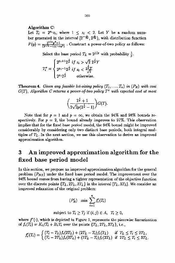
3 An improved approximation algorithm for the fixed base period model In this section, we propose an improved approximation algorithm for the general problem (Plvs) under the fixed base period model. The improvement over the 94% bound comes from having a tighter representation of the objective function over the discrete points {TL, 2TL, 3TL} in the interval [TL, 3TL]. We consider an improved relaxation of the original problem:

n

(P~) min ~ f [ ( T i ) i = l

subject to 7~ > 7~ if (i, j) e A, 7] >_ 0,

where if(.), which is depicted in Figure 1, represents the piecewise linearization of fi(Ti) = Ki/Ti + HiTi over the points {TL, 2TL, 3TL}, i.e.,

f~(7~) = ( (7] - TL)f~(2TL) + (2TL -- 7~)f~(TL) if TL < T~ < 2TL, (T~ 2Tz.)fi(3TL) + (3TL - Ti)fi(2TL) if 2TL < Ti < 3TL.

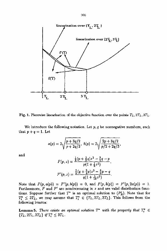
366

l ineTzat ion over tTL, 2T L ]

/ / linearization over [2Tt~ 3T~

i i i . . . . . . . . . . . . . j . . . . .

[ T L 2 T L 3 T L

Fig. 1. Piecewise linearization of the objective function over the points TL, 2TL, 3T~.

We introduce the following notation. Let p, q be nonnegative numbers, such that p + q = 1. Let

and

2" ~ o / 2p + 3q/2 ~ = V p--4-~q/3' b(p) = ,V~,/-/-~2-~- 3,

- - - ~ q - - p F(p,z) "- ~(p+ "~q)z2 3

- - ~ p - q F'(p,z)= ~(q+ ap)z2 4 q(1 + ~z2)

Note that F(p,a(p)) = F'(p,b(p)) = 0, and f (p ,b(p)) = F'(p, 2a(p)) = 1. Furthermore, F and F' are nondecreasing in z and are valid distribution functions. Suppose further that T* is an optimal solution to (P~). Note that for T~' < 3TL, we may assume that Ti* e {TL, 2TL, 3TL}. This follows from the following lemma:

L e m m a 5. There exists an optimal solution T* with the property that Ti* E {TL, 2TL, 3TL} if T~* <_ 3TL.

367

Consider the following rounding algorithm:

A l g o r i t h m D: Let p = 0.7, q = 0.3. Let a = a(0.7) and b = b(0.3). Note that a < b < 2a. Select Policy 1 below with probability p, and Policy 2 with probability q. Pol icy 1: Let Ti* = 2P~TLzi, where zi is in the interval [1, 2). Let Y be a random number generated in the interval [a(p), b(p)] with distribution function F(p, y). Let

{2e~TL if2zi < Y, T/I = 2P~+ITL if2zi > Y.

Pol icy 2: Let Ti* = 3.2P'TLZ~, where z~ is in the interval [1, 2). Let Y' be a random number generated in the interval [b(p), 2a(p)] with distribution function F'(p, y). For Ti > 3TL, let

{3.2PiTL if3z~ < Y', 7'2 = 3.2P'+ITL if3z~ > Y'.

For all items i with 7} = 2TL, we round them (simultaneously) to 3TL with probability ~ and to TL with probability ~4" Note that in this way, for T / = 2TL,

E(T~) 8 = 2TLE(1_). -

Finally, if Ti* - TL, Ti 2 -- TL.

Let T denote the vector of ordering intervals under the selected policy.

T h e o r e m 6. The expected cost of the policy T produced by algorithm D is at most 1.043 times the value of the continuous relaxation (P~).

Proof : Without loss of generality, we assume TL = 1. If Ti* = 2, then

E(Ti - 2TLE( ~--~) = p+ 8q = 1.0428...

Thus we only need to consider the ease when Ti* greater than 3. Suppose Ti* lies in (1) [2k'a, 2k'b] or (2) (2k'b, 2k'+la]. In case (1), Policy 2 always rounds 7~ to 3 . 2 k~, whereas in case (2), Policy 1 always rounds Ti to 2 k~+~. Case ( 1 ) : T/* lies in [2V'a, 2V'b], i.e., T/* = 2V'wi, where wi E [a, hi. Then

E(Ti) = pE(T2) + qE(T?) = T/* (3q + p2(1 + F(p, wi))), wi wi

368

and

E ( ~i = P E ( ~'~sl ) + q E ( ~---~s~ ) =1"-~'7 i ( q "w . +p(1 F ( p , w ,

We have chosen F(p, .) such that

3 + F(p, wi)) wi F(p, w,) q - - + p2(1 = q-~- + p(1 )wi/2. w~ w~ 2

With this choice of F(p, .), and p = 0.7, q = 0.3, we can optimize the bound over the range of w~ to obtain

E(7 ) - - ~ = T ; E ( ~ ) < 1.043.

Case (2) : Ti* lies in (2P'b, 2P~+la], i.e. T* = 2P~wi where wi e (b, 2a]. Then

E(pT: + qT?) = r*(p~w ~ + q3(1 + F'(p, wi))), r

and 1 , 3wi F'( wi))wi/3). E ( P ~---[,I + q ~-~.2 ) = "~ t P -'4 "- + q (1 2

We have chosen F~(p, .) such that

P~w/4 + q3(1 + F~(P,wi wi)) = P'-4"3wi + q(1 Fl(~w~))wi/3.

With this choice of F'(p, .), again we have

E(pT~ + qT~ 2) . 1 1 = E(p + < 1.043 T,*

Hence the result follows. []

We next show that if T i" > v~Ts for all i we can improve the approximation guarantee. This result will be useful in the next section. We consider the following modified rounding algorithm:

A l g o r i t h m E: Let p = 0.5, q = 0.5. Select Policy 1 with probability p and Policy 2 otherwise: Pol icy 1: The same as in Algorithm D. Pol icy 2: For Ti* > 3TL, the same as in Algorithm D. For Ti* in [V~TL, 3TL], we round T~ to 3TL.

The following result follows from a similar analysis to Theorem 6.

T h e o r e m 7. If T~ >__ v~TL for all i, then the expected cost of the policy T obtained from Algorithm E is at most 1.031 times the optimal value of the continuous relaxation ( PR).

369

4 An improved approximation algorithm for the (OWMR) problem In this section we improve the guarantee of 1.043 to 1.031 for the problem of a single warehouse supplying and distributing items to a group of n retailers. For distribution systems Roundy [18] has showed that the optimal nested policy can be arbitrarily bad compared to the optimal stationary policy. Under the assumption that the retailers place their order only when their inventory level is zero, he showed that there is an optimal stationary policy which satisfies the integer ratio property, i.e., the ratio of the ordering interval T/ for retailer i and the ordering interval To of the warehouse is either an integer or 1 over an integer. He has also constructed similar 94% and 98% approximation algorithms for problem (OWMR), with fixed and variable base period respectively.

The problem can be modelled as follows (see [18]):

n n

(PowMR) min C(T)= ~ ( K J T / ) + Z ( g , max(To,~) + H{~) i..~O i----1

subject to ~00 E {ki, :ki integer},

T/ integer for all i = 0, . n, T L ~ ~ '

where g, - �89 hod,, and Hi -- �89 ( h, - ho)d,. We consider the following relaxation:

n . n

(PRowMR) min ~(K, /T~) + ~ ( g , max(T0,T/) + HIT/) i = 0 i----1

subject to T/ _ TL for all i = 0 , . . . , n.

The constraint T / > TL is a relaxation of the condition that each T/is an integral multiple of TL. Let T/*, i = 0, l , . . . , n be a solution of the relaxation (PRowMR).

In this section, we improve on the approximation bound for the fixed base period model, by using six stronger relaxations. These relaxations correspond to the requirement that either T~) ~_ 6TL or T~) = kTL for k in {1, 2, 3, 4, 5}.

We first consider the relaxation

n

(Ps) Zs -- m i n { Z ( f ~ ( ~ ) +g/max(T0,T/)) +go~To: TO >_ 6TL,Ti >_ TL}, i----1

where f~(T/) = fi(Ti) -- Ki /T/+ Hi~ if T/ >_ 3TL, and f~(T~) is the piecewise linearization of f~(T/) over the points {TL, 2TL, 3TL}. Note that this relaxation provides a lower bound to the optimal value of (PowMR). Z6 can be computed in O(n) time by using a linear time median finding algorithm, as suggested in

370

Queyranne [15] or Lu Lu and Posner [12]. Let T/* be the optimal solution of relaxation (P6). Following Lemma 5 we may assume that T/* e {Ts 2TL, 3TL) if T/* < 3TL. We apply Algorithm E that leaves those T* with values TL or 2TL unchanged.

L e m m a 8. Algorithm E applied to an optimal solution to relaxation (P6) produces an integer ratio policy with cost within 1.031 of Z6.

Proof: Policies 1 and 2 of Algorithm E round those T/* with values greater than or equal to 3TL to a power-of-two policy of the type 2PITL or 2P~(3TL). Those T/* with values TL or 2TL are left unchanged. The expected gap between T/* and the rounded value 7} again satisfies

E(1/7}) E(7}) < 1.031, < 1.031.

T/* - l / T * -

Note that in addition, because of the dependence in the rounding process,

E[max(7], T0)] = max(E[7}], E[T0])I < 1.031 max(T/*, T~).

Note that since T~ > 6TL, T~ is rounded to a multiple of 4TL (under Policy 1) or multiples of 6TL (under Policy 2). Therefore, the policy constructed need not satisfy the condition To > 6TL, since Policy 1 might round T~ down to 4TL. However, the policy obtained is an integer ratio policy. [3

We next consider the case that T~ = kTL, k E {1,2,3,4,5}. Let f~(Ti) denote a partial piecewise linearization of fi(7}) in the interval [TL, 3kTL], over the points TL, kTL,2kTL, 3kTL. Particularly for k = 4, in addition to TL, 4TL, 8TL, 12TL we include the point 2TL in the linearization. For k E {1, 2, 3, 4, 5} we consider the following five relaxations, in which we fix the value of To to be kTL and consider the linearization f~ (7}) instead of fl (Ti):

n

(Pk) Zk = rain{Ca(T) = Ko/(kTL) + ~ ( g l max(kTL, 7}) q- f~ (7~)) : !/} >_ TL}. i = l

Note that each relaxation can be solved in O(n). Moreover,

L e m m a 9. There exists an optimal solution T k fo Zk with the property that if T/~ < 3kTL, then

T~' ~ {TL, kTL, 2kTL, 3kTL} for k = 1, 2, 3, 5

T~ ~ {TL, 2TL, 4TL, 8TL, 12TL} for k = 4.

We next show that Algorithm E applied to the optimal solution of relaxation (Pk) produces an integer ratio policy within 1.031 of Z~.

371

L e m m a 10. For k = 1 , . . . , 5 Algorithm E applied to an optimal solution of relaxation ( Pk ) that satisfies Lemma 9 produces an integer ratio policy with cost within 1.031 of Z~.

Combining Lemmas 8 and 10 we obtain

T h e o r e m 11. For the one-warehouse-multi-retailer problem with fixed base period, there is an O(n) time 96.9~ approximation algorithm.

5 E x t e n s i o n s

Since our prior analysis did not utilize any structure of the optimal solution, our proof techniques cover several extensions of the basic models almost effort- lessly. Our techniques produce randomized rounding algorithms for the following problems considered in the literature:

1. Capacitated lot-sizing problems, in which we add constraints 21~TL < 7] < 2mTL for each i. Since the Algorithms A and B preserve these properties, Theorems 1 and 2 apply also for this capacitated version of the problem, giving rise to 94% and 98% power-of-two policies respectively. The same result was also derived in Federgruen and Zheng [6] by extending Roundy's approach to the capacitated version.

2. Submodular ordering costs introduced in Federgruen et al. [5] and Zheng [211:

(PsuB) Z = minmax XJ'( k--i + HIT/) T

T~ _<Tj if (/ , j) c A ,

T / > T/; for each i. k E P ,

where P - - {k: Z k j < K(S), Z kj = K(N),kj > 0},

j@S jEN

and K(S) submodular. Algorithms A and B can be used to round the fractional optimal solution in (PsuB) to 94% and 98% optimal power-of- two solutions. Furthermore, if T/* _> v~TL for all i, then the fixed base period bound can be improved further to 96.9%, using Theorem 7.

3. Resource constrained lot-sizing problems considered in Roundy [20], in which we add to (PNs) constraints of the type

aij/7~ < Ai, i = 1, . . . ,m. J

372

He showed that there is a power-of-two policy for the variable base period case with cost at most 1.44 times the optimal solution. We can generalize this result to the lot-sizing problems with submodular joint cost function. Consider the following algorithm:

A l g o r i t h m F: Let (k*, T*) be an optimal solution to (PsuB) with the resource constraints added. Use Tj = V~Tj* in Algorithm B to obtain a power-of-two policy T ~ .

First note that Tf lies in the interval [Tj/v/'2, TjV~] and hence Tj ~ > Tj*. Therefore, T/~ satisfies the resource constraints.

T h e o r e m 12. Let T* be an optimal solution to the resource constrained version of (PsuB). Using Algorithm F on T*, we obtain a power-of-two policy with cost at most 1.44 times of the optimal.

Proof : Since scaling by v~ does not affect the ordering of T~, the solution k* is also a maximum solution to G(T~ Therefore, the result follows directly from the following observation:

and

1 -T" = 1----V~T.* ~ 1.44Tj* E(T;) < V log(2) v log(2)

< 1 1

D

References

1. D. Atkins, M. Queyrarme and D. Sun. Lot sizing policies for finite production rate assembly systems, Operations Research, 40, 126-141, 1992.

2. D. Bertsimas, C. Teo and R. Vohra. Nonlinear relaxations and improved randomized approximation algorithms for multicut problems, Proc. 4th IPCO Conference, 29-39, 1995.

3. D. Bertsimas and R. Vohra. Linear programming relaxations, approximation al- gorithras and randomization : a unified view of covering problems, Preprint 1994.

4. G. Dobson. The Economic Lot-Scheduling Problem: Achieving Feasibility using Time-Varying Lot Sizes, Operations Research, 35, 764-771, 1987.

5. A. Federgruen, M. Queyranne and Y.S. Zheng. Simple power-of-two policies are close to optimal in a general class of production/dlstrlbution system with general joint setup costs, Mathematics of Operations Research, 17, 4, 1992.

373

6. A. Federgruen and Y.S. Zheng. Optimal power-of-two replenishment strategies in capacitated general production/distribution networks, Management Science, 39, 6, 710-727, 1993.

7. M.X. Goemans and David Williamson. A new 3/4 approximation algorithm for MAX SAT, Proc. 3rd IPCO Conference, 313-321, 1993.

8. M.X. Goemans and David Williamson..878 approximation algorithms for MAX- CUT and MAX 2SAT, Proc. 26th Annual ACM STOC, 422-431, 1994.

9. D. Hochbaum and G. Shanthikumar. Convex separable optimization is not much harder than linear optimization, Journal o] ACM, 37, 843-861, 1990.

10. P. Jackson, W. Maxwell and J. Muckstadt. The joint replenishment problem with power-of-two restriction. AIIE Trans., 17, 25-32, 1985.

11. P. Jackson and R. Roundy. Minimizing separable convex objective on arbitrarily directed trees of variable upperbound constraints, Mathematics of Operations Research, 16, 504-533, 1991.

12. Lu Lu and M. Posner. Approximation procedures for the one-warehouse multi- retailer system, management Science, 40, 1305-1316, 1994.

13. W.L. Maxwell and J.A. Muckstadt. Establishing consistent and realistic reorder intervals in Production-distribution systems, Operations Research, 33, 1316-1341, 1985.

14. J.A. Muckstadt and R.O. Rotmdy. Analysis of Multisatage Production Systems, in: S.C. Graves, A.H.G. Rirmooy Kan and P.H. Zipkin (ed.) Logistics of Production and Inventory, North Holland, 59-131, 1993.

15. M. Queyrarme. Finding 94%-effective policies in linear time for some production/inventory systems, Unpublished manuscript, 1987.

16. P. Raghavan and C. Thompson. Randomized rounding : a technique for provably good algorithms and algorihmic proofs, Combinatorica 7, 365-374, 1987.

17. M. Rosenblatt and M. Kaspi. A dynamic programming algorithm for joint replenishment under general order cost functions, Management Science, 31, 369-373, 1985.

18. R.O. Roundy. 98% Effective integer-ratio lot-sizing for one warehouse multi- retailer systems, Management Science, 31(11),1416-1430, 1985.

19. R.O. Roundy. A 98% Effective lot-sizing rule for a multi-product, multi-stage production inventory system, Mathematics of Operations Research, 11, 699-727, 1986.

20. R.O. Roundy. Rounding off to powers of two in continuous relaxations of capacitated lot sizing problems, Management Science, 35, 1433-1442, 1989.

21. Y.S. Zheng. Replenishment strategies for production/distribution networks with general joint setup costs, Ph.D. Thesis, Columbia University, New York, 1987.

Documents

Improved randomized approximation algorithms for lot-sizing …dbertsim/papers/ApproximationAlgorithms/Improved... · Improved Randomized Approximation Algorithms for Lot-Sizing Problems