Embed Size (px)
Citation preview

TREBALL FINAL DE GRAU
TÍTOL DEL TFG: Time to land prediction based on machine learning
models TITULACIÓ: Grau en Enginyeria d’Aeronavegació AUTOR: Àlex Asenjo Carvajal DIRECTOR: Cristina Barrado Muxi DATA: 17 de juliol de 2020

Títol: Time to land prediction based on machine learning models Autor: Àlex Asenjo Carvajal Director: Cristina Barrado Muxi Data: 17 de juliol de 2020
Resumen
El objetivo de éste trabajo final de grado es evaluar diferentes modelos de machine learning (ML) para predecir el tiempo que tardará en aterrizar cualquier avión en el aeropuerto de Josep Tarradellas Barcelona-El Prat. Para tener una mejor idea de lo que es realmente el ML y como se puede usar en el campo de la gestión del tráfico aéreo (ATM), se ha hecho una breve introducción de los diferentes tipos de aprendizaje que existen además de la mención de las diferentes áreas de influencia de éste tipo de algoritmos en proyectos impulsados por el programa Europeo de I+D en ATM Single European Sky ATM Research Joint Undertaking (SESAR JU), como por ejemplo, mejorar la predicción de tráfico, el flujo de pasajeros en aeropuertos y la eficiencia de las operaciones aéreas. Para alcanzar el objetivo del proyecto, la mayor parte de los datos, con los que más tarde se alimentarán los algoritmos, se han extraído de mensajes ADS-B sin procesar. Parte de estos datos como coordenadas, alturas, etc. se han extraído de manera directa de los reportes ADS-B mientras que otra información como la categoría de estela turbulenta (WTC), la pista de aterrizaje y los datos meteorológicos, se han obtenido de manera indirecta a partir de otros datos de los reportes y mediante el uso de diferentes bases de datos. En cuanto a las conclusiones obtenidas al final del proyecto, el mejor modelo hallado para predecir el tiempo de aterrizaje de los aviones con destino el aeropuerto Josep Tarradellas Barcelona-El Prat, ha sido el RandomForestRegressor, siendo un tipo de aprendizaje supervisado y, como su nombre indica, basado en la regresión. Aparte de ser el modelo más preciso y exacto, es el que presenta menores tiempos de fit y score, siendo parámetros clave para una hipotética implementación real. Finalmente, y en aras de no descartar ninguna posibilidad de mejora, es probable la obtención de mejores modelos mediante el uso de una mayor potencia computacional debido a la alta exigencia de recursos requeridos en algunas partes del proyecto.


Title: Time to land prediction based on machine learning models Author: Àlex Asenjo Carvajal Director: Cristina Barrado Muxi Date: July 17th, 2020
Overview
The aim of the present Bachelor Final Project is to evaluate different machine learning (ML) models to predict the time any aircraft would take to land at Josep Tarradellas Barcelona-El Prat Airport.
To get a better picture of what ML really is and how it can be used in the air traffic management (ATM) field, a brief introduction of the different types of learning apart from viewing the areas of influence of this type of algorithms in some projects driven by the European R&D ATM program SESAR JU such as improving traffic predictability, enhancing the passenger flow in airports and improving airport operations’ performance.
To achieve the goal of the project, raw ADS-B messages sent by nearby aircraft of the airport have been used as the main source of information from which various ML algorithms have been fed with. Part of the data extracted from those messages like coordinates, altitudes, etc. have been used directly after being correspondingly processed and other type of information like the wake turbulence category (WTC), the landing runway and the meteorology have been obtained from indirect deduction from other fields of ADS-B messages and by using various databases. Regarding the conclusions obtained at the end of this project, the best model found to predict the time any aircraft attempting to land at Josep Tarradellas Barcelona-El Prat Airport would need to do so is the RandomForestRegressor, being a supervised learning type of ML and as its name suggests, a regression-based model. Apart from being the most precise and accurate model, it is also the one with the most reasonable fit and score time, being key parameters when talking about a hypothetical actual implementation. Finally, so as not to not discard any options for improvement, it is probable that better solutions can be achieved with the use of higher computational power due to the amount of calculations needed for some parts of the project.

INDEX
INTRODUCTION ................................................................................................ 1
CHAPTER 1. MACHINE LEARNING .............................................................. 3
1.1 Introduction to Machine Learning .................................................................... 3 1.1.1 Types of Machine Learning Systems ...................................................... 3
1.2 ML on ATM ......................................................................................................... 6 1.2.1 Traffic predictability .................................................................................. 6 1.2.2 Passenger flow at airports ....................................................................... 7 1.2.3 Airport operations .................................................................................... 7 1.2.4 Recent investigations............................................................................... 7
1.3 Tools and models .............................................................................................. 8 1.3.1 Scikit-learn ............................................................................................... 8 1.3.2 Models ..................................................................................................... 8 1.3.3 Splitter methods ..................................................................................... 10 1.3.4 Hyper-parameter optimizers .................................................................. 13 1.3.5 Metrics ................................................................................................... 13 1.3.6 Evaluation & Validation .......................................................................... 14
1.4 Methodology .................................................................................................... 15
CHAPTER 2. DATA COLLECTION AND PREPARATION .......................... 16
2.1 Data collection ................................................................................................. 16 2.1.1 Flightradar24 .......................................................................................... 16 2.1.2 ADS-B Antenna ..................................................................................... 16 2.1.3 Bleriot ..................................................................................................... 18
2.2 Data pre-processing ........................................................................................ 19 2.2.1 ADS-B Decoder ..................................................................................... 19 2.2.2 Dataset creation ..................................................................................... 22
2.3 Data filtering and preparation ........................................................................ 26 2.3.1 Numerical features ................................................................................. 26 2.3.2 Categorical features............................................................................... 27 2.3.3 Dataset overview ................................................................................... 27
CHAPTER 3. RESULTS................................................................................ 29
CHAPTER 4. CONCLUSIONS ...................................................................... 35
BIBLIOGRAPHY .............................................................................................. 36
LIST OF FIGURES Fig. 1.1 Supervised learning .............................................................................. 4 Fig. 1.2 Unsupervised learning .......................................................................... 5 Fig. 1.3 Semi-supervised learning ...................................................................... 5 Fig. 1.4 Reinforced learning ............................................................................... 6 Fig. 1.5 One hidden layer MLP .......................................................................... 9
Fig. 1.6 Random forest scheme ....................................................................... 10 Fig. 1.7 Train_test_split scheme ...................................................................... 11 Fig. 1.8 Stratified Shuffle Split scheme ............................................................ 12 Fig. 1.9 Categories generated to preserve the proportions of samples ............ 12 Fig. 1.10 Methodology scheme ........................................................................ 15
Fig. 2.1 Radarcape setup scheme ................................................................... 17 Fig. 2.2 Decoder IP address without receiving flights. ..................................... 17
Fig. 2.3 Reduction in the number of operations during the second half of March .................................................................................................................. 18
Fig. 2.4 Data pipeline ....................................................................................... 19 Fig. 2.5 Sample of an already encoded file ...................................................... 21
Fig. 2.6 KML file generated from the CSV file .................................................. 21 Fig. 2.7 Flight trajectory of an aircraft. Landings highlighted ............................ 23
Fig. 2.8 False landings ..................................................................................... 23 Fig. 2.9 Example of the aircraft positioning: ARP distance of 67,916km and ARP
azimuth of 79,85º ...................................................................................... 24
Fig. 2.10 Result of the data processing and preparation .................................. 28 Fig. 3.1 Cross-validation evaluation of RMSE and R2 ...................................... 30 Fig. 3.2 Cross-validation evaluation of fit and score times ............................... 31
Fig. 3.3 Cross-validation RMSE, % of under RMSE, 𝑅2 and 𝑅2 ...................... 32
Fig. 3.4 Known vs. predicted TTL. Case 3.3.1 ................................................. 33
Fig. 3.5 Prediction error histogram ................................................................... 34
Fig. 3.6 Go-around ........................................................................................... 34

LIST OF TABLES Table 2.1 Relation of ADS-B fields and information extracted ......................... 19 Table 2.2 Different unit cells structure and format. Unit cell of line 1 is not
repeated .................................................................................................... 20
ACRONYMS, ABBREVIATIONS AND DEFINITIONS ADS-B Automatic Dependent Surveillance – Broadcast AI Artificial Intelligence AMSL Above Mean Sea Level ANN Artificial Neural Network ARP Airport Reference Point ASR Automatic Speech Recognition ATM Air Traffic Management ETA Estimated Time of Arrival LNA Low Noise Amplifier GS Ground Speed HCA Hierarchical Cluster Analysis IAS Indicated Airspeed IP Internet Protocol MAHALO Modern ATM via Human/Automation Learning Optimization METAR Meteorological Aerodrome Report ML Machine Learning MLP Multi-layer Perceptron NaN Not a Number NAS Network Attached Storage OLS Ordinary Least Squares PCA Principal Component Analysis RMSE Root-Mean-Square Error SESAR JU Single European Sky ATM Research Joint Undertaking STAR Standard Terminal Arrival Route TAS True Airspeed TTL Time to land UPS Uninterruptible Power Supply

ACKNOWLEDGEMENTS I would like to greatly thank my family and friends for being there for these four years. I also want to express my gratitude to my tutor Cristina Barrado Muxi, whose support and dedication made it possible and to Enric Pastor, Xavier Prats, Marcos Pérez, Daniel García-Monteavaro, Jaune Assens y Francesc Fernandez for their contribution to the project.

INTRODUCTION 1
INTRODUCTION In the last decade, followed by the improvement of the calculation capacity, the field of the Artificial Intelligence (AI) and its subfields have suffered a boom. With the implementation of new ML algorithms, modern problems now can be tackled in a more efficient way such as object, facial and voice recognition software that automatically improves over time. In the last lustrum, the SESAR JU program has implemented AI and ML in many projects with the objective of solving complex problems such as traffic predictability or improving airport operations with the common objective of increasing the efficiency and lowering the costs of an increasingly complex European network. Airports rely on control centres and ultimately on the control tower to manage and sequence incoming flights. Besides flight trajectory prediction software to forecast the volume of arrivals, it is very useful for air traffic controllers to have an additional dimension to sequence arrivals: the time. A very useful tool to help air traffic controllers in the process of sequencing incoming aircraft to their final approach path in the most efficient way could be adding this fourth dimension to offer a consistent way of arrival flights’ sequencing and thus, reducing controller’s workload. It is in this context where this project rises. The final objective is offering the estimated time of arrival (ETA) of flights landing at Josep Tarradellas Barcelona-El Prat Airport with the implementation of ML models. To accomplish that the project aims towards predicting the time to land (TTL) of those flights and thus, deducing its ETA. The project is structured in three main chapters: Chapter one introduces the basis of ML and describes the influence, contribution and possibilities of ML in the European ATM. It also presents the software used, Scikit-learn, and its many implemented features, tools and models. The closure of this chapter explains the methodology used to determine which of the ML models is the best in predicting the TTL. Chapter two describes each step of data acquisition needed to feed the models. Starting with data acquisition from raw ADS-B reports from a local network server and concluding with data pre-processing, filtering and preparation to fit ML algorithms’ requirements. The third and final chapter is focused in extracting all the results and considering the key parameters that could affect the final decision such as the overall performance of each model and the time required to fit and evaluate the model. Far from perfection this project hopes to contribute the philosophy of the ML and apply it to improve the existing infrastructure. The main code of the project is uploaded to GitHub repository: https://github.com/alexasenjo/TFG-library.git.

2 Time to land prediction based on machine learning models

MACHINE LEARNING 3
CHAPTER 1. MACHINE LEARNING
This chapter introduces the basis of ML, its applications and capabilities and the tools and used to implement it in the current project.
1.1 Introduction to Machine Learning
ML is a branch of AI based in computer algorithms with the ability to parse data, learn from it and then make prediction from new data. The concept was first introduced by Arthur Samuel in 1952 when he wrote a program to play the game of draughts and learn the more it played by implementing a search tree [1] and choosing its next move over a minimax [2] strategy.
1.1.1 Types of Machine Learning Systems
Depending on which type of data will be used as input, needed as output or simply by the type of problem is meant to solve, there are many different approaches. The most frequently used are:
• Supervised learning
• Unsupervised learning
• Semi-supervised learning
• Reinforcement learning
1.1.1.1 Supervised learning
This type of ML is characterized by the inclusion of the desired output (label) that the model is meant to predict within the training set. This type of approach is widely used to solve classification and regression problems where a discrete categorization or a numeric value has to be predicted, respectively. The most important supervised learning models are:
• Linear Regression
• Neural Networks1
• Decision Trees and Random Forest The dataset is the information which the model is fed with and is composed of three main elements:
• Labels: the value to predict. In this project is the TTL.
• Features: each characteristic chosen (position, altitude, etc.).
• Instances: each flight of the dataset that contains all the features plus the label.
1 Some neural network architectures can be unsupervised, such as autoencoders and restricted Boltzmann machines. They can also be semi-supervised, such as in Deep belief networks and unsupervised pretraining.
4 Time to land prediction based on machine learning models
In this fashion, the dataset is a 𝑛 × 𝑚 matrix where 𝑛 is the number of instances
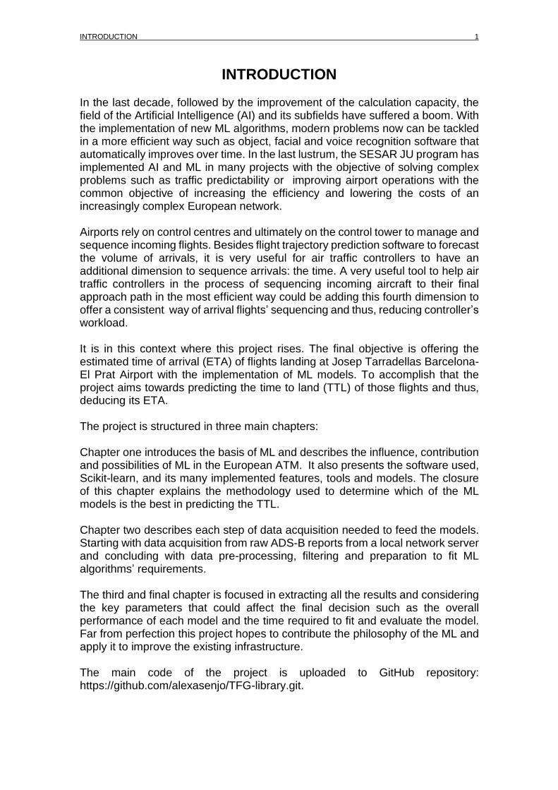
and 𝑚 is the number of features plus one (in this case there is only one label per instance). It is very important to mention why it is necessary to split the dataset in two subsets: the training and the test set. The training set is used to fit the model and its labels are used to adjust it. The test set is used to evaluate the model and its labels are not passed to the model, instead, they are used to validate the predictions done by the model. Fig. 1.1 illustrates the concept of any supervised learning model and the proper use of the training and test set.
Fig. 1.1 Supervised learning
1.1.1.2 Unsupervised learning
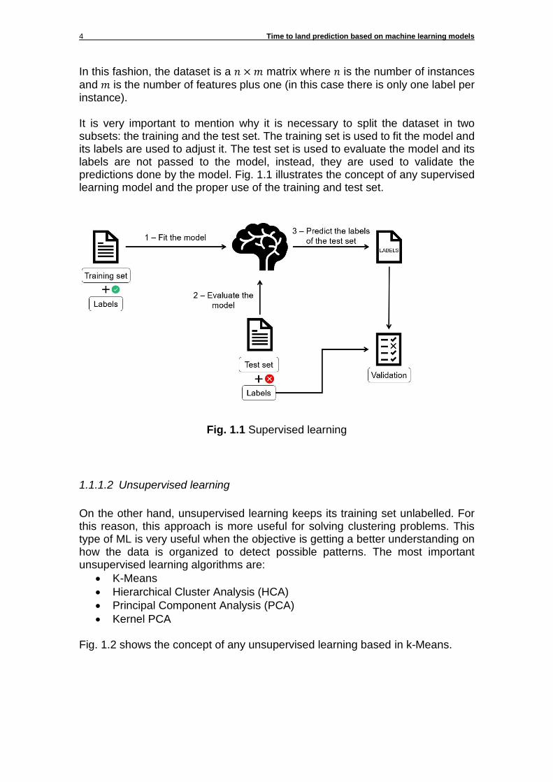
On the other hand, unsupervised learning keeps its training set unlabelled. For this reason, this approach is more useful for solving clustering problems. This type of ML is very useful when the objective is getting a better understanding on how the data is organized to detect possible patterns. The most important unsupervised learning algorithms are:
• K-Means
• Hierarchical Cluster Analysis (HCA)
• Principal Component Analysis (PCA)
• Kernel PCA Fig. 1.2 shows the concept of any unsupervised learning based in k-Means.
MACHINE LEARNING 5
Fig. 1.2 Unsupervised learning
1.1.1.3 Semi-supervised learning
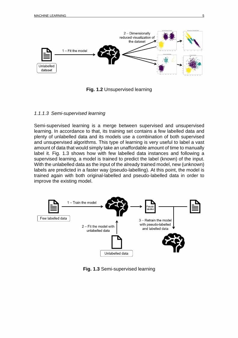
Semi-supervised learning is a merge between supervised and unsupervised learning. In accordance to that, its training set contains a few labelled data and plenty of unlabelled data and its models use a combination of both supervised and unsupervised algorithms. This type of learning is very useful to label a vast amount of data that would simply take an unaffordable amount of time to manually label it. Fig. 1.3 shows how with few labelled data instances and following a supervised learning, a model is trained to predict the label (known) of the input. With the unlabelled data as the input of the already trained model, new (unknown) labels are predicted in a faster way (pseudo-labelling). At this point, the model is trained again with both original-labelled and pseudo-labelled data in order to improve the existing model.
Fig. 1.3 Semi-supervised learning
6 Time to land prediction based on machine learning models
1.1.1.4 Reinforcement learning
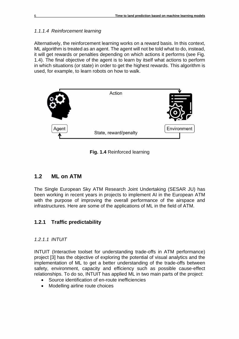
Alternatively, the reinforcement learning works on a reward basis. In this context, ML algorithm is treated as an agent. The agent will not be told what to do, instead, it will get rewards or penalties depending on which actions it performs (see Fig. 1.4). The final objective of the agent is to learn by itself what actions to perform in which situations (or state) in order to get the highest rewards. This algorithm is used, for example, to learn robots on how to walk.
Fig. 1.4 Reinforced learning
1.2 ML on ATM
The Single European Sky ATM Research Joint Undertaking (SESAR JU) has been working in recent years in projects to implement AI in the European ATM with the purpose of improving the overall performance of the airspace and infrastructures. Here are some of the applications of ML in the field of ATM.
1.2.1 Traffic predictability
1.2.1.1 INTUIT
INTUIT (Interactive toolset for understanding trade-offs in ATM performance) project [3] has the objective of exploring the potential of visual analytics and the implementation of ML to get a better understanding of the trade-offs between safety, environment, capacity and efficiency such as possible cause-effect relationships. To do so, INTUIT has applied ML in two main parts of the project:
• Source identification of en-route inefficiencies
• Modelling airline route choices
MACHINE LEARNING 7
1.2.1.2 COPTRA
COPTRA (Combining Probable Trajectories) project [4] has the objective of predicting the flight trajectory closer to the take-off. The actual implementation of ML in this project is to predict the speed at any given moment of the climb phase of the take-off in order to further estimate the occupancy of determined air-sectors near airports.
1.2.2 Passenger flow at airports
1.2.2.1 BigData4ATM [5]
With the big data phenomenon and with the use of ML techniques, this project aims towards analysing and combining passenger-centric geo-located data with other more traditional demographic and economic data to inform ATC decision-making processes.
1.2.3 Airport operations
1.2.3.1 MALORCA
MALORCA (Machine Learning of Speech Recognition Models for Controller Assistance) project [6] designed a ML based solution to improve ATC communications in order to avoid manual input of ATC commands with the implementation of automatic speech recognition (ASR).
1.2.4 Recent investigations
1.2.4.1 MAHALO
MAHALO (Modern ATM via Human/Automation Learning Optimization) project [7] aims towards an explainable system for problem solving between aircrew and ATC with the implementation of ML. It is expected to increase the airspace capacity, performance and safety. It will also investigate how well the ML decisions are explained to the ATC in order understand the decision making of the algorithm and the conformity of the decisions, that is, the similarity between AI and ATC decisions.
8 Time to land prediction based on machine learning models
1.3 Tools and models
1.3.1 Scikit-learn
Scikit-learn is an open source python-based library which provides various tools to implement ML algorithms. It is a good starting point to begin any ML project due to its wide range of tools and functions. Scikit-learn offers a wide variety of ML models in addition to a great repository of common ML practices as model fitting, data pre-processing and model selection and evaluation among other.
1.3.2 Models
Considering the type of problem intended to solve, the most convenient type of learning is clearly the supervised one since the label or the value to predict is clearly defined (TTL) and the fact this value is a continuous numeric one, regression models will be used.
1.3.2.1 Linear Regression
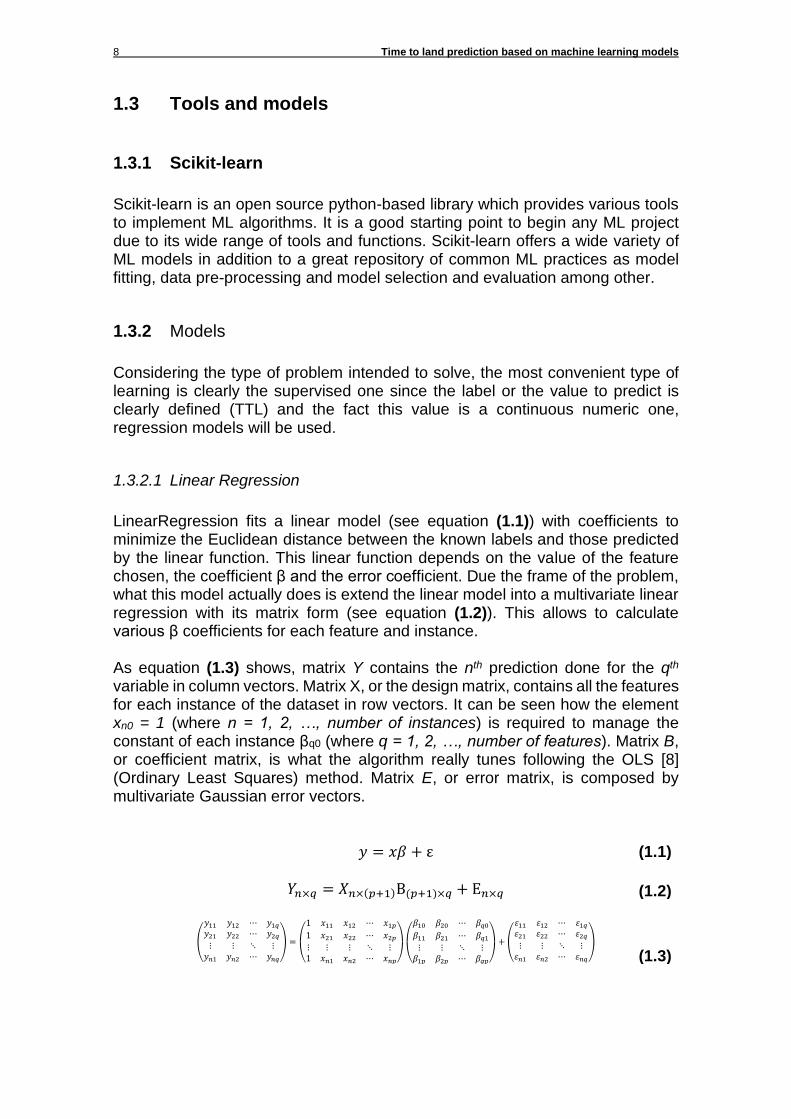
LinearRegression fits a linear model (see equation (1.1)) with coefficients to minimize the Euclidean distance between the known labels and those predicted by the linear function. This linear function depends on the value of the feature chosen, the coefficient β and the error coefficient. Due the frame of the problem, what this model actually does is extend the linear model into a multivariate linear regression with its matrix form (see equation (1.2)). This allows to calculate various β coefficients for each feature and instance. As equation (1.3) shows, matrix Y contains the nth prediction done for the qth variable in column vectors. Matrix X, or the design matrix, contains all the features for each instance of the dataset in row vectors. It can be seen how the element xn0 = 1 (where n = 1, 2, …, number of instances) is required to manage the constant of each instance βq0 (where q = 1, 2, …, number of features). Matrix B, or coefficient matrix, is what the algorithm really tunes following the OLS [8] (Ordinary Least Squares) method. Matrix E, or error matrix, is composed by multivariate Gaussian error vectors. 𝑦 = 𝑥𝛽 + ε (1.1)
𝑌𝑛×𝑞 = 𝑋𝑛×(𝑝+1)Β(𝑝+1)×𝑞 + Ε𝑛×𝑞 (1.2)
(
𝑦11 𝑦12 ⋯ 𝑦1𝑞𝑦21 𝑦22 ⋯ 𝑦2𝑞⋮ ⋮ ⋱ ⋮𝑦𝑛1 𝑦𝑛2 ⋯ 𝑦𝑛𝑞
) =
(
1 𝑥11 𝑥12 ⋯ 𝑥1𝑝1 𝑥21 𝑥22 ⋯ 𝑥2𝑝⋮ ⋮ ⋮ ⋱ ⋮1 𝑥𝑛1 𝑥𝑛2 ⋯ 𝑥𝑛𝑝)
(
𝛽10 𝛽20 ⋯ 𝛽𝑞0𝛽11 𝛽21 ⋯ 𝛽𝑞1⋮ ⋮ ⋱ ⋮𝛽1𝑝 𝛽2𝑝 ⋯ 𝛽𝑞𝑝)
+ (
𝜀11 𝜀12 ⋯ 𝜀1𝑞𝜀21 𝜀22 ⋯ 𝜀2𝑞⋮ ⋮ ⋱ ⋮𝜀𝑛1 𝜀𝑛2 ⋯ 𝜀𝑛𝑞
) (1.3)
MACHINE LEARNING 9
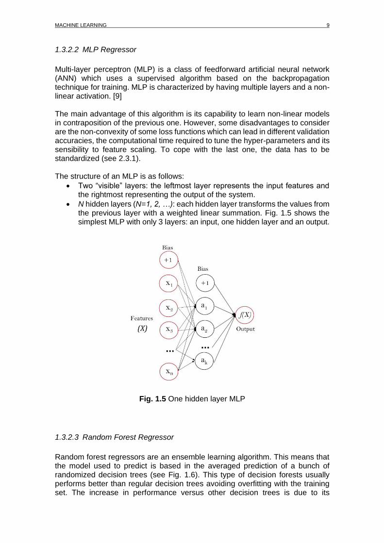
1.3.2.2 MLP Regressor
Multi-layer perceptron (MLP) is a class of feedforward artificial neural network (ANN) which uses a supervised algorithm based on the backpropagation technique for training. MLP is characterized by having multiple layers and a non-linear activation. [9] The main advantage of this algorithm is its capability to learn non-linear models in contraposition of the previous one. However, some disadvantages to consider are the non-convexity of some loss functions which can lead in different validation accuracies, the computational time required to tune the hyper-parameters and its sensibility to feature scaling. To cope with the last one, the data has to be standardized (see 2.3.1). The structure of an MLP is as follows:
• Two “visible” layers: the leftmost layer represents the input features and the rightmost representing the output of the system.
• N hidden layers (N=1, 2, …): each hidden layer transforms the values from the previous layer with a weighted linear summation. Fig. 1.5 shows the simplest MLP with only 3 layers: an input, one hidden layer and an output.
Fig. 1.5 One hidden layer MLP
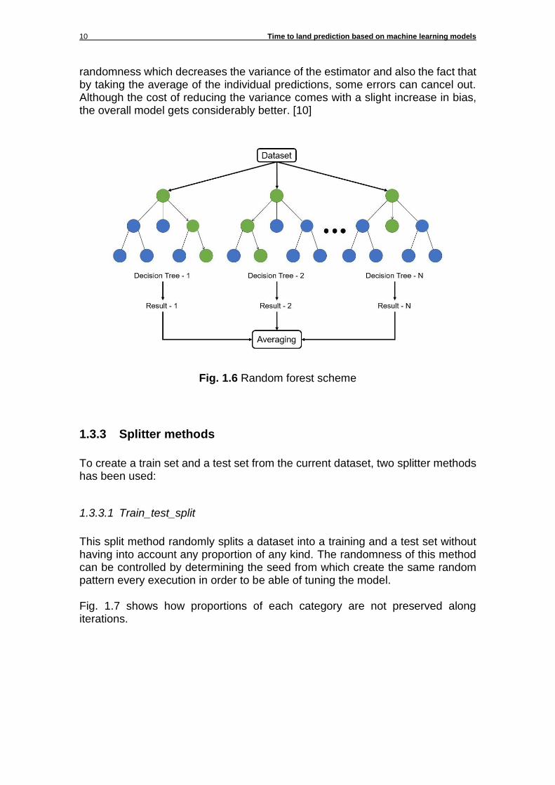
1.3.2.3 Random Forest Regressor
Random forest regressors are an ensemble learning algorithm. This means that the model used to predict is based in the averaged prediction of a bunch of randomized decision trees (see Fig. 1.6). This type of decision forests usually performs better than regular decision trees avoiding overfitting with the training set. The increase in performance versus other decision trees is due to its
10 Time to land prediction based on machine learning models
randomness which decreases the variance of the estimator and also the fact that by taking the average of the individual predictions, some errors can cancel out. Although the cost of reducing the variance comes with a slight increase in bias, the overall model gets considerably better. [10]
Fig. 1.6 Random forest scheme
1.3.3 Splitter methods
To create a train set and a test set from the current dataset, two splitter methods has been used:
1.3.3.1 Train_test_split
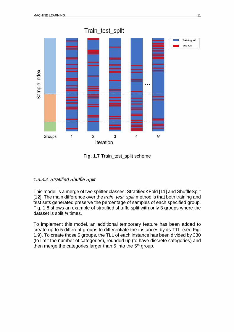
This split method randomly splits a dataset into a training and a test set without having into account any proportion of any kind. The randomness of this method can be controlled by determining the seed from which create the same random pattern every execution in order to be able of tuning the model. Fig. 1.7 shows how proportions of each category are not preserved along iterations.
MACHINE LEARNING 11
Fig. 1.7 Train_test_split scheme
1.3.3.2 Stratified Shuffle Split
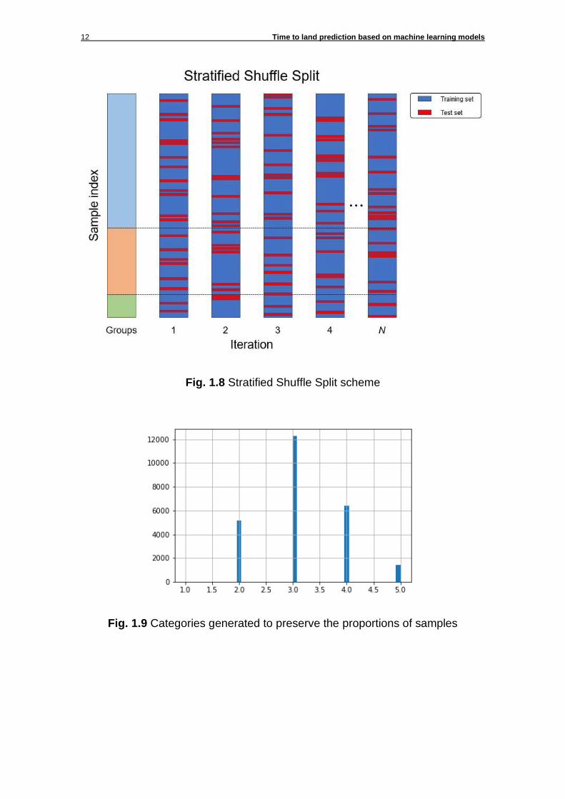
This model is a merge of two splitter classes: StratifiedKFold [11] and ShuffleSplit [12]. The main difference over the train_test_split method is that both training and test sets generated preserve the percentage of samples of each specified group. Fig. 1.8 shows an example of stratified shuffle split with only 3 groups where the dataset is split N times. To implement this model, an additional temporary feature has been added to create up to 5 different groups to differentiate the instances by its TTL (see Fig. 1.9). To create those 5 groups, the TLL of each instance has been divided by 330 (to limit the number of categories), rounded up (to have discrete categories) and then merge the categories larger than 5 into the 5th group.
12 Time to land prediction based on machine learning models
Fig. 1.8 Stratified Shuffle Split scheme
Fig. 1.9 Categories generated to preserve the proportions of samples
MACHINE LEARNING 13
1.3.4 Hyper-parameter optimizers
Scikit-learn offers many methods to tune estimators. For this task, two of them have been chosen: GridSearchCV and RandomizedSearchCV.
1.3.4.1 GridSearchCV
This method is an exhaustive way to try and evaluate the response of the estimator with determined values specified with the param_grid parameter. When a GridSearchCV element is fitted with a dataset, all possible combinations of the estimator parameters specified in the param_grid are evaluated and the best combination of parameters is used to predict new values. One major drawback of this method is that due its combinational nature, it’s execution can be very time-consuming if the number of elements contained in the param_grid is not especially taken into account.
1.3.4.2 RandomizedSearchCV
Like the previous method, this one evaluates a certain number of estimators with different parameter configurations in order to retain the best one. However, it has some benefits over the exhaustive search given its randomness:
• The budget can be selected regardless of the number of parameters of the estimator and its possible values. To do so, scipy.stats module provides many distributions for sampling parameters and generate independent random samples on consecutive calls.
• There is no performance penalty in the addition of parameters without influence in the model.
1.3.5 Metrics
1.3.5.1 RMSE RMSE is the measure of the average error committed, in this case, in a prediction. RMSE is a common metric to measure the overall accuracy of the model. In
equation (1.4), �̂�𝑛 is the predicted value of the 𝑛𝑡ℎ instance, 𝑦𝑛 is the label or real value of the same instance and 𝑁 is the total number of instances.
𝑅𝑀𝑆𝐸 = √∑ (�̂�𝑛 − 𝑦𝑛)2𝑁𝑛=1
𝑁
(1.4)

14 Time to land prediction based on machine learning models
1.3.5.2 𝑅2 and adjusted 𝑅2
As its name implies, the adjusted 𝑅2 is a correction of the𝑅2 [13]. 𝑅2 (also known as coefficient of determination) measures the proportion of the variance in the label that is predictable from the features of the instances, that is, the correlation between features and labels. Its scale is measured in percentage from 0 (totally uncorrelated) to 100% (totally correlated). The drawback of 𝑅2 is that in basically
every regression model, by adding features, the value of the 𝑅2 increases, giving the false impression of improving the model.
To solve this, the 𝑎𝑑𝑗𝑢𝑠𝑡𝑒𝑑 𝑅2 (or �̅�2) considers the impact of the number of features in the correlation. By doing this, it gives a better idea of how much of the
correlation is due the addition of “extra” variables. �̅�2 increases when the number
of features in the correlation enhances the value of the 𝑅2 and decreases when
the number of features is inflating the value of 𝑅2 meaningless. (1.5) shows the
expression of �̅�2 where 𝑛 is the number of instances and 𝑝 is the number of
features used in the prediction. The value of 𝑅2 is automatically computed by the built-in Scikit-learn tools.
�̅�2 = 1 −(1 − 𝑅2)(𝑛 − 1)
𝑛 − 𝑝 − 1
(1.5)
1.3.6 Evaluation & Validation
Scikit-learn functions cross_validate and cross_val_predict have been used to respectively evaluate and validate each model and configuration.
1.3.6.1 Cross_validate
Very similar to another built-in function called cross_val_score, this one allows for multiple metrics to be evaluated and also returns fit-times, score-times and test-scores.
1.3.6.2 Cross_val_predict
Its basis is very similar to the cross_validate function but in this case, the output is the predicted value input when the instance is in the test set. Its main function is to visualize the predictions of different models.
MACHINE LEARNING 15
1.4 Methodology
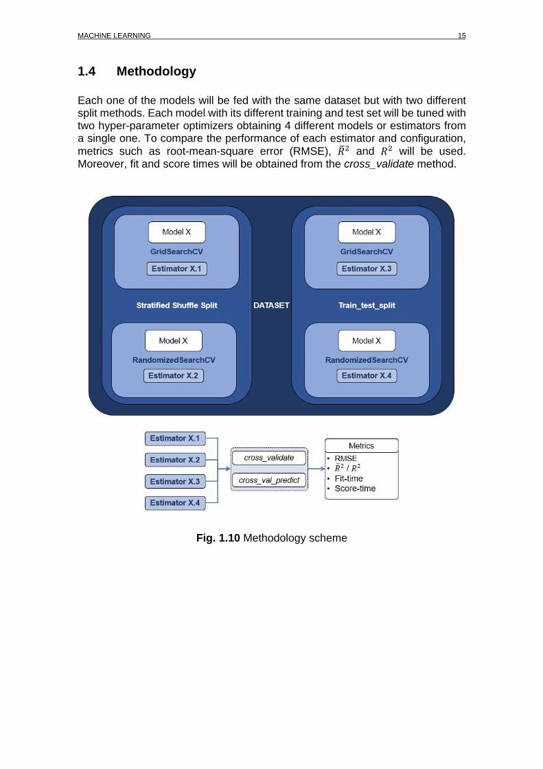
Each one of the models will be fed with the same dataset but with two different split methods. Each model with its different training and test set will be tuned with two hyper-parameter optimizers obtaining 4 different models or estimators from a single one. To compare the performance of each estimator and configuration,
metrics such as root-mean-square error (RMSE), �̅�2 and 𝑅2 will be used. Moreover, fit and score times will be obtained from the cross_validate method.
Fig. 1.10 Methodology scheme
16 Time to land prediction based on machine learning models
CHAPTER 2. DATA COLLECTION AND PREPARATION This chapter presents the process of getting the raw data from Automatic Dependent Surveillance – Broadcast (ADS-B) reports, processing it to extract the relevant information and final preparation to fit the requirements of the ML algorithms.
2.1 Data collection
For any ML model, one of the most important elements is the data with which will be fed. At a first glance it seems a good idea to use the ADS-B Mode-S reports sent by the aircraft to any nearby ground station since those reports contain relevant information of each aircraft such as the speed, the position, the altitude, the heading, etc. To minimize some of the avoidable biases it is very important to consider a dataset big enough to be able of training and then evaluate the model properly. The appropriate size of the dataset highly depends on the complexity of the problem so to keep it simple, in this particular case the amount of data to use will be as large as possible.
2.1.1 Flightradar24
A feasible way to obtain flight information was flightradar24’s webpage. This portal shares an historical database of flights from up to 3 years ago. In this case the amount of data available is vast. However, the fact that each flight had to be downloaded one by one and the daily limit of 60 downloads per day made this not a viable option. It would take more than 5 months and a half just to collect a 10,000 flights dataset.
2.1.2 ADS-B Antenna
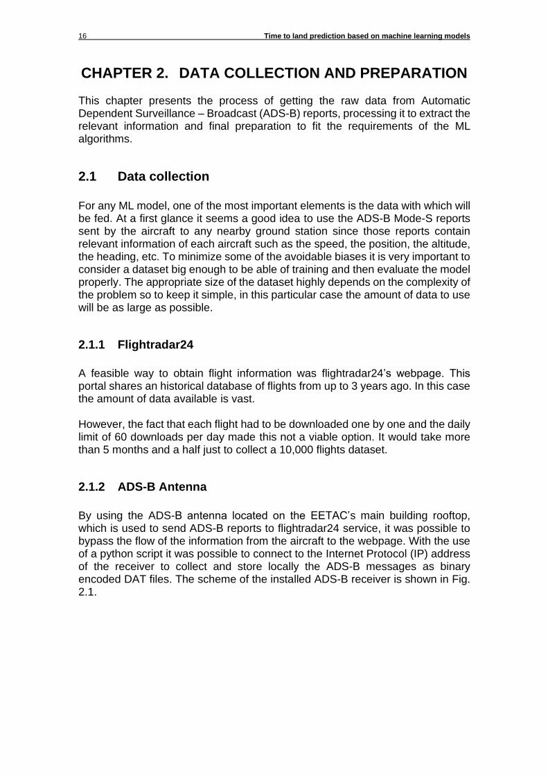
By using the ADS-B antenna located on the EETAC’s main building rooftop, which is used to send ADS-B reports to flightradar24 service, it was possible to bypass the flow of the information from the aircraft to the webpage. With the use of a python script it was possible to connect to the Internet Protocol (IP) address of the receiver to collect and store locally the ADS-B messages as binary encoded DAT files. The scheme of the installed ADS-B receiver is shown in Fig. 2.1.
DATA COLLECTION AND PREPARATION 17
Fig. 2.1 Radarcape setup scheme
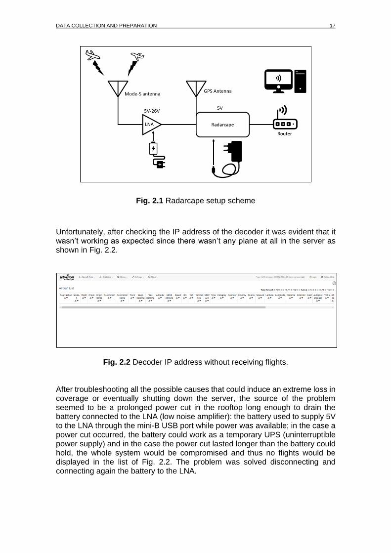
Unfortunately, after checking the IP address of the decoder it was evident that it wasn’t working as expected since there wasn’t any plane at all in the server as shown in Fig. 2.2.
Fig. 2.2 Decoder IP address without receiving flights.
After troubleshooting all the possible causes that could induce an extreme loss in coverage or eventually shutting down the server, the source of the problem seemed to be a prolonged power cut in the rooftop long enough to drain the battery connected to the LNA (low noise amplifier): the battery used to supply 5V to the LNA through the mini-B USB port while power was available; in the case a power cut occurred, the battery could work as a temporary UPS (uninterruptible power supply) and in the case the power cut lasted longer than the battery could hold, the whole system would be compromised and thus no flights would be displayed in the list of Fig. 2.2. The problem was solved disconnecting and connecting again the battery to the LNA.
18 Time to land prediction based on machine learning models
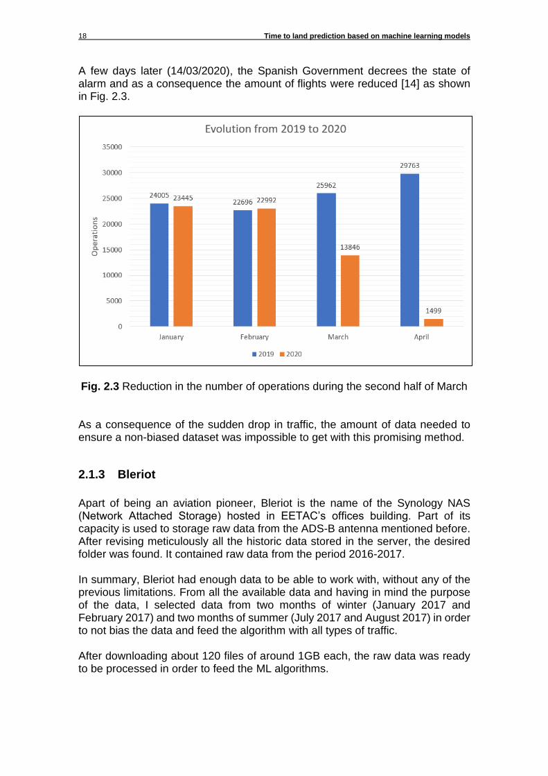
A few days later (14/03/2020), the Spanish Government decrees the state of alarm and as a consequence the amount of flights were reduced [14] as shown in Fig. 2.3.
Fig. 2.3 Reduction in the number of operations during the second half of March As a consequence of the sudden drop in traffic, the amount of data needed to ensure a non-biased dataset was impossible to get with this promising method.
2.1.3 Bleriot
Apart of being an aviation pioneer, Bleriot is the name of the Synology NAS (Network Attached Storage) hosted in EETAC’s offices building. Part of its capacity is used to storage raw data from the ADS-B antenna mentioned before. After revising meticulously all the historic data stored in the server, the desired folder was found. It contained raw data from the period 2016-2017. In summary, Bleriot had enough data to be able to work with, without any of the previous limitations. From all the available data and having in mind the purpose of the data, I selected data from two months of winter (January 2017 and February 2017) and two months of summer (July 2017 and August 2017) in order to not bias the data and feed the algorithm with all types of traffic. After downloading about 120 files of around 1GB each, the raw data was ready to be processed in order to feed the ML algorithms.
DATA COLLECTION AND PREPARATION 19
2.2 Data pre-processing
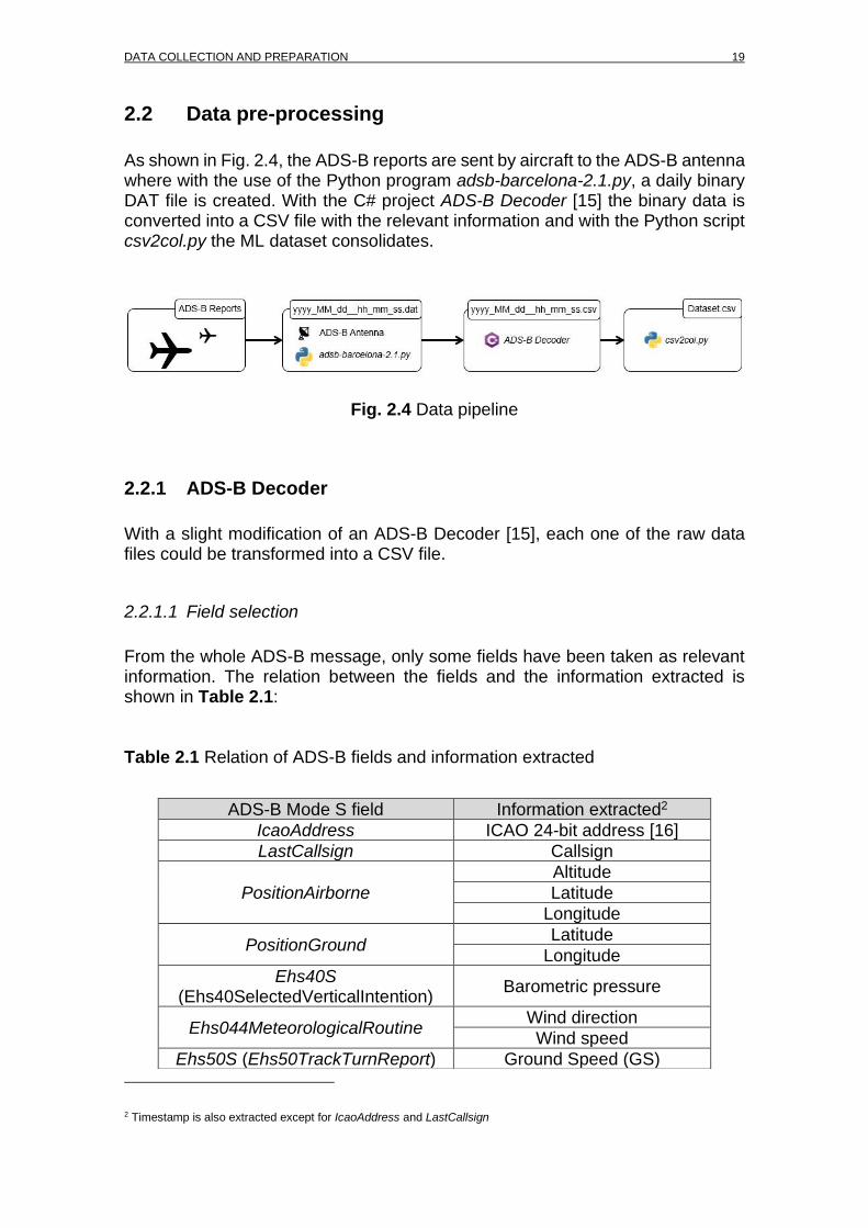
As shown in Fig. 2.4, the ADS-B reports are sent by aircraft to the ADS-B antenna where with the use of the Python program adsb-barcelona-2.1.py, a daily binary DAT file is created. With the C# project ADS-B Decoder [15] the binary data is converted into a CSV file with the relevant information and with the Python script csv2col.py the ML dataset consolidates.
Fig. 2.4 Data pipeline
2.2.1 ADS-B Decoder
With a slight modification of an ADS-B Decoder [15], each one of the raw data files could be transformed into a CSV file.
2.2.1.1 Field selection
From the whole ADS-B message, only some fields have been taken as relevant information. The relation between the fields and the information extracted is shown in Table 2.1: Table 2.1 Relation of ADS-B fields and information extracted
2 Timestamp is also extracted except for IcaoAddress and LastCallsign
ADS-B Mode S field Information extracted2
IcaoAddress ICAO 24-bit address [16]
LastCallsign Callsign
PositionAirborne
Altitude
Latitude
Longitude
PositionGround Latitude
Longitude
Ehs40S (Ehs40SelectedVerticalIntention)
Barometric pressure
Ehs044MeteorologicalRoutine Wind direction
Wind speed
Ehs50S (Ehs50TrackTurnReport) Ground Speed (GS)
20 Time to land prediction based on machine learning models
2.2.1.2 Data structure
The data has been structured in a certain way in order to cope with the variability in length of the data or the total absence of it as some of the fields are not mandatory but valuable enough to consider them. The type of format chosen is CSV because it allows the visualization of the data using a spreadsheet in order to check in a fast manner if the data consistency was enough to be used later. The way the information is arranged inside the file have been done having in mind the later processing with csv2col.py. The file structure is based on the repetition of a unit cell. This unit cell is composed of 8 lines and each of them is the repetition of a different unit cell except the line containing the callsign and the ICAO code. Table 2.2 shows every unit cell of which the file is made of. Table 2.2 Different unit cells structure and format. Unit cell of line 1 is not repeated
Flight unit cell
Line No. Field unit cell
1 Callsign; ICAO 24-bit address
2 Heading; Timestamp
3 Latitude; Longitude; Altitude [ft];
Timestamp
4 Latitude; Longitude; Timestamp
5 IAS [kt]; Timestamp
6 Barometric pressure [hPa]; Timestamp
7 Wind direction; Wind speed [kt];
Timestamp
8 GS [kt]; TAS [kt]; Timestamp
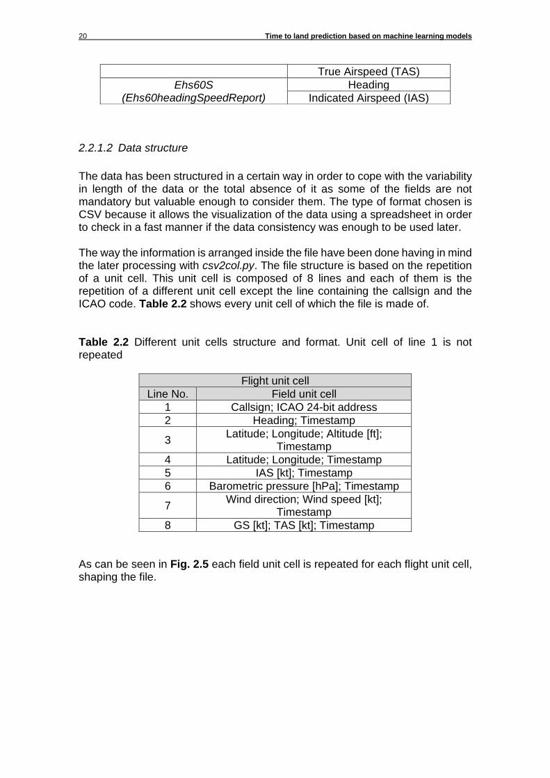
As can be seen in Fig. 2.5 each field unit cell is repeated for each flight unit cell, shaping the file.
True Airspeed (TAS)
Ehs60S (Ehs60headingSpeedReport)
Heading
Indicated Airspeed (IAS)
DATA COLLECTION AND PREPARATION 21
Fig. 2.5 Sample of an already encoded file
2.2.1.3 KML generation
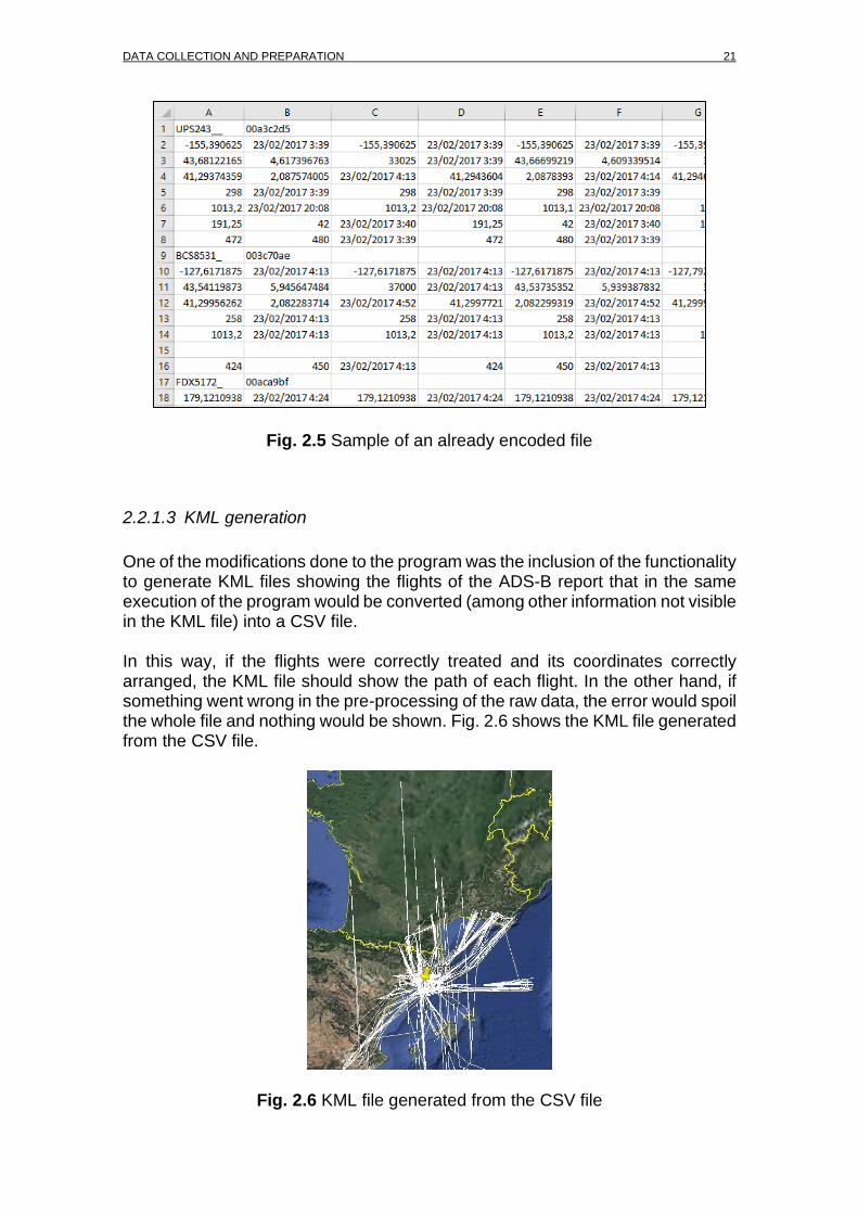
One of the modifications done to the program was the inclusion of the functionality to generate KML files showing the flights of the ADS-B report that in the same execution of the program would be converted (among other information not visible in the KML file) into a CSV file. In this way, if the flights were correctly treated and its coordinates correctly arranged, the KML file should show the path of each flight. In the other hand, if something went wrong in the pre-processing of the raw data, the error would spoil the whole file and nothing would be shown. Fig. 2.6 shows the KML file generated from the CSV file.
Fig. 2.6 KML file generated from the CSV file
22 Time to land prediction based on machine learning models
2.2.2 Dataset creation
The main purpose of this program is to convert the considerable size of most of the fields into individual alphanumeric values that will be contained in the matrix that later on will feed the ML model.
2.2.2.1 Flight identification
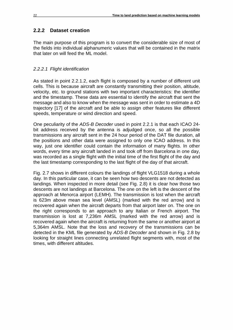
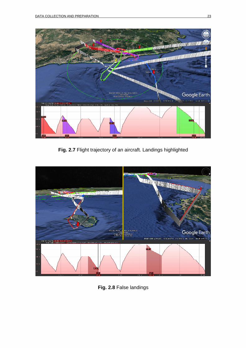
As stated in point 2.2.1.2, each flight is composed by a number of different unit cells. This is because aircraft are constantly transmitting their position, altitude, velocity, etc. to ground stations with two important characteristics: the identifier and the timestamp. These data are essential to identify the aircraft that sent the message and also to know when the message was sent in order to estimate a 4D trajectory [17] of the aircraft and be able to assign other features like different speeds, temperature or wind direction and speed. One peculiarity of the ADS-B Decoder used in point 2.2.1 is that each ICAO 24-bit address received by the antenna is adjudged once, so all the possible transmissions any aircraft sent in the 24 hour period of the DAT file duration, all the positions and other data were assigned to only one ICAO address. In this way, just one identifier could contain the information of many flights. In other words, every time any aircraft landed in and took off from Barcelona in one day, was recorded as a single flight with the initial time of the first flight of the day and the last timestamp corresponding to the last flight of the day of that aircraft. Fig. 2.7 shows in different colours the landings of flight VLG1518 during a whole day. In this particular case, it can be seen how two descents are not detected as landings. When inspected in more detail (see Fig. 2.8) it is clear how those two descents are not landings at Barcelona. The one on the left is the descent of the approach at Menorca airport (LEMH). The transmission is lost when the aircraft is 623m above mean sea level (AMSL) (marked with the red arrow) and is recovered again when the aircraft departs from that airport later on. The one on the right corresponds to an approach to any Italian or French airport. The transmission is lost at 7,236m AMSL (marked with the red arrow) and is recovered again when the aircraft is returning from the same or another airport at 5,364m AMSL. Note that the loss and recovery of the transmissions can be detected in the KML file generated by ADS-B Decoder and shown in Fig. 2.8 by looking for straight lines connecting unrelated flight segments with, most of the times, with different altitudes.
DATA COLLECTION AND PREPARATION 23
Fig. 2.7 Flight trajectory of an aircraft. Landings highlighted
Fig. 2.8 False landings
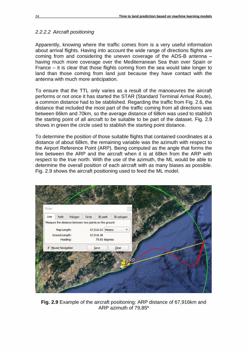
24 Time to land prediction based on machine learning models
2.2.2.2 Aircraft positioning
Apparently, knowing where the traffic comes from is a very useful information about arrival flights. Having into account the wide range of directions flights are coming from and considering the uneven coverage of the ADS-B antenna – having much more coverage over the Mediterranean Sea than over Spain or France – it is clear that those flights coming from the sea would take longer to land than those coming from land just because they have contact with the antenna with much more anticipation. To ensure that the TTL only varies as a result of the manoeuvres the aircraft performs or not once it has started the STAR (Standard Terminal Arrival Route), a common distance had to be stablished. Regarding the traffic from Fig. 2.6, the distance that included the most part of the traffic coming from all directions was between 66km and 70km, so the average distance of 68km was used to stablish the starting point of all aircraft to be suitable to be part of the dataset. Fig. 2.9 shows in green the circle used to stablish the starting point distance. To determine the position of those suitable flights that contained coordinates at a distance of about 68km, the remaining variable was the azimuth with respect to the Airport Reference Point (ARP). Being computed as the angle that forms the line between the ARP and the aircraft when it is at 68km from the ARP with respect to the true north. With the use of the azimuth, the ML would be able to determine the overall position of each aircraft with as many biases as possible. Fig. 2.9 shows the aircraft positioning used to feed the ML model.
Fig. 2.9 Example of the aircraft positioning: ARP distance of 67,916km and ARP azimuth of 79,85º
DATA COLLECTION AND PREPARATION 25
2.2.2.3 Feature selection
At this point, the features extracted from the original raw data are the minimum to identify each flight and the bare minimum information as the initial position with respect to the airport. However, the number of features needed to adequately train a ML model has to be grater and give some type of extra information. Flights are already divided into one at a time arrival flights but with the unique built-in feature of the timestamp. The use of the timestamp makes feasible to pick what information is needed from the ADS-B message codified in the CSV file. In this way, fields as “Heading”, “Altitude”, “IAS” and “GS” were added to the matrix (the value of each field when the flight was at 68km of the ARP). Other features needed some preparation as for example, the meteorology. This one is a very useful feature since the weather is a key factor in the capacity of any airport and can determine whether the ATC gives shortcuts or holdings in the approach. Unfortunately, this information was very scarce in the ADS-B messages as it is not a mandatory field. To tackle this inconvenient, a local DDBB was created by downloading the meteorological aerodrome reports (METAR) (from December 2016 to November 2017) from OGIMET’s webpage. With each flight initial timestamp, it was possible to find the appropriate METAR and parse its information: “Barometric pressure”, “Wind direction”, “Wind variability”, “Wind speed” and “Visibility”. Another important aspect to consider when scheduling arrivals is the minimum distance needed between different aircraft types in order to sequence them for the final approach. With the available data, the mix index is the most suitable metric that shows the overall aircraft type mixing that the airspace has. Equation (2.1) shows the expression to compute the mix index [18] where C is the percent of class C or smaller aircraft and D is the percent of class D or greater aircraft. 𝑀𝑖𝑥 𝑖𝑛𝑑𝑒𝑥 (%) = (𝐶 + 3𝐷) (2.1)
To compute the mix index, it is necessary to know the WTC [19] of each aircraft. After a lot of research, it was possible to know the aircraft model and type by searching the ICAO 24-bit address in an online database. One problem was the time required to search one by one each aircraft and saving the useful information in a local database. This problem was solved by coding a custom web scraper [20] to automate the whole process. However, a limit of 150 queries per day limited the speed of the overall process. After some days executing the web scraper code with most of the aircraft, a local database containing ICAO 24-bit addresses and its aircraft type and WTC was created. In this way, the code could be executed as many times as necessary without the dependence of a third-party software. In any case, if necessary, the web scraper code is executed automatically by the program if an unparsed aircraft is detected and adds it to the local database for the next execution.
26 Time to land prediction based on machine learning models
By using the callsign of each aircraft, the airline of each flight could be extracted and used in the ML model. As using each different airline as a different feature would be tedious and useless for the ML (adding many features/columns without adding much information is counterproductive), a merging of airlines into four groups was the best option to store this information and, in this way, it could be even more useful. Those four groups referred to four different regions from all over the world that implies a very different type of traffic: European, North American, South American and other airlines. With the adequate treat of the last coordinates of each flight and crossing them with the positions of each runway threshold, it was possible to extract the runway of each flight in a consistent way. In this way, it could be seen if there is more preferability by ATC to give more shortcuts in any specific runway making the time to land lower. Additionally, the day of the week of each flight was added to the features of the matrix due its simplicity and the fact that could bring light to know if exists any pattern of congestion that leads to a lower rate of shortcuts before or after the weekends, for example.
2.3 Data filtering and preparation
Until this point, every transformation has been done with the purpose of better understanding the data and its meaning but, from now on, each transformation will aim towards adapting the data for the requirements of ML algorithms. Some Scikit-learn built-in functions and utilities will be used.
2.3.1 Numerical features
To work properly, any ML algorithm needs a robust dataset and, as the size of the dataset is big enough to make unfeasible a strict check of the values, it is highly advisable to implement an automatic method to standardize the data. The first step is to be sure that all the numeric values are, in fact, numbers. By using a pipeline [21], the implementation of an imputer [22] was direct: if any value of the dataset (from those features specified as numbers) is detected as a NaN (Not a Number) type, that NaN value will be replaced by the median of the values of that same numeric feature that are not NaN. The second and the last step in the processing of numerical features is to standardize the data. The aim of this step is to make the data more manageable for most part of the algorithms and leading into better solutions. One possible solution could be using the “MinMaxScaler” [23] function that consists in the scaling of all the values from 0 to 1. The major drawback of this method is its sensitivity to outliers. The appearance of a single outlier could represent the condensation of the relevant data in a much narrower margin leading in a possible worsening of the results. In the other hand, the “StandardScaler” [24] function transforms the data in a such way that its distribution has a mean value of 0 and
DATA COLLECTION AND PREPARATION 27
a standard deviation of 1. This means that the scale differences between features (e.g. “Initial_time” values range from 0 to 86400s while “Day_of_the_week” goes from 0 to 6 and “Mix_index” values can be up to 300) can be removed in order to compare its values without compromising the data. It is very important to ensure that the function “StandardScaler” is used properly. To not condition the results, it is indispensable to fit the scaler to the training set only, and once the scaler has been trained, transform the training set and the test set using the same scale. So, in this case, if the scaler is fitted with both training and test set, the performance of the model will be unbeatable just because you are asking the same questions you made to tune the model.
2.3.2 Categorical features
Categorical or alphanumeric attributes need a special care in order to be used. Those categorical attributes are “WTC” and “RWY”. With the implementation of a “LabelBinarizer” [25] it is possible to convert each categorical feature into as many binary rows as categories it has. In this way, the feature “RWY” is transformed into 5 independent columns or new features each one indicating every available runway: 02, 07L, 07R, 25L and 25R. The “WTC” feature is split into L (Light), M (Medium), H (Heavy) and J (Super). This categorization has been done according to the ICAO standard [26].
2.3.3 Dataset overview
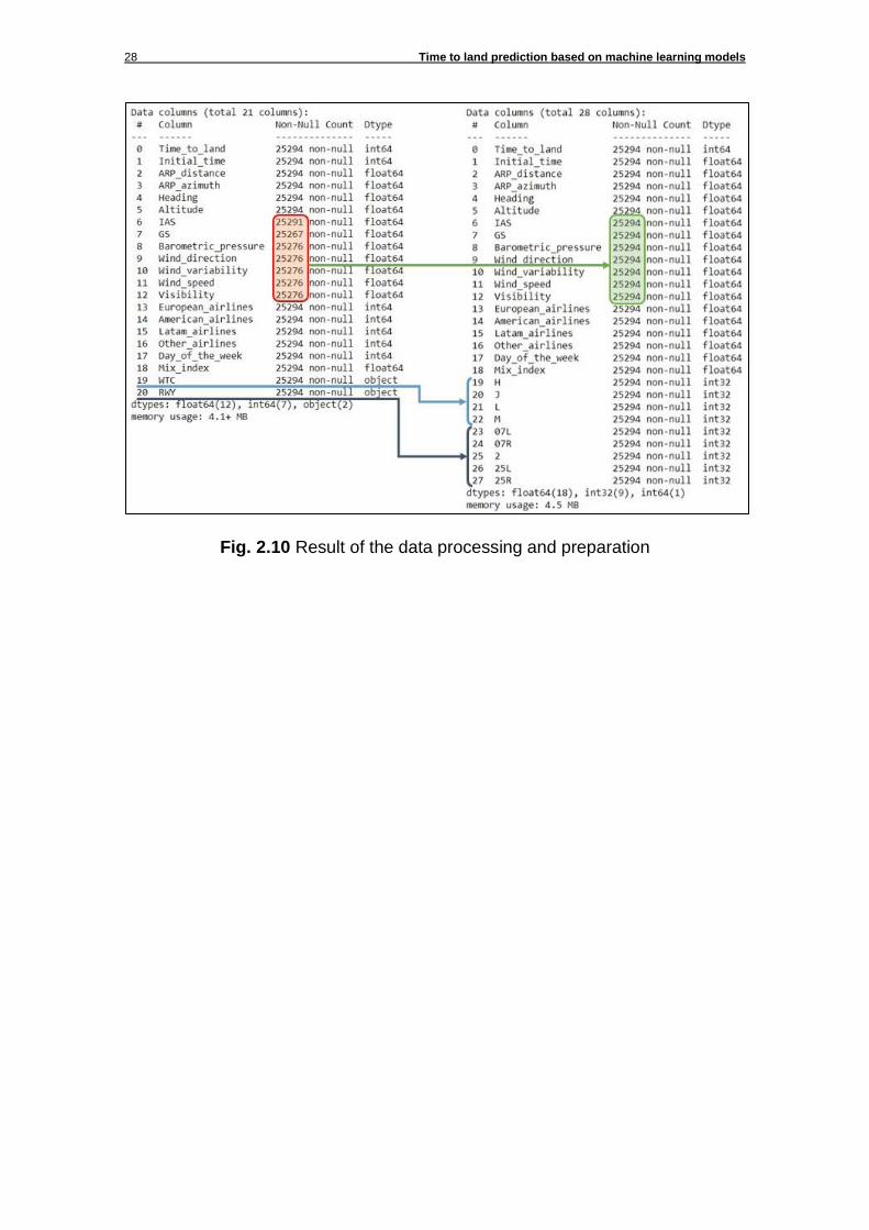
As can be seen in Fig. 2.10, after processing the data with the Scikit-learn library, now all features have the same number of non-null elements thanks to the imputer. Moreover, the total number of features seems to have 9 more elements although being the expansion of the categorical features as explained in 2.3.2.
28 Time to land prediction based on machine learning models
Fig. 2.10 Result of the data processing and preparation
RESULTS 29
CHAPTER 3. RESULTS The following structure has been used to establish a context from which to refer each different model and configuration: 1. Linear Regression
1.1. StratifiedShuffleSplit 1.1.1. GridSearchCV 1.1.2. RandomizedSearchCV
1.2. Train_test_split 1.2.1. GridSearchCV 1.2.2. RandomizedSearchCV
1.3. Cross-validation 1.3.1. Estimator A (1.1.1) 1.3.2. Estimator B (1.1.2) 1.3.3. Estimator C (1.2.1) 1.3.4. Estimator D (1.2.2)
2. MLP Regressor 2.1. StratifiedShuffleSplit
2.1.1. GridSearchCV 2.1.2. RandomizedSearchCV
2.2. Train_test_split 2.2.1. GridSearchCV
2.2.2. RandomizedSearchCV 2.3. Cross-validation
2.3.1. Estimator E (2.1.1) 2.3.2. Estimator F (2.1.2) 2.3.3. Estimator G (2.2.1) 2.3.4. Estimator H (2.2.2)
3. Random Forest Regressor 3.1. StratifiedShuffleSplit
3.1.1. GridSearchCV 3.1.2. RandomizedSearchCV
3.2. Train_test_split 3.2.1. GridSearchCV 3.2.2. RandomizedSearchCV
3.3. Cross-validation 3.3.1. Estimator I (3.1.1) 3.3.2. Estimator J (3.1.2) 3.3.3. Estimator K (3.2.1) 3.3.4. Estimator L (3.2.2)
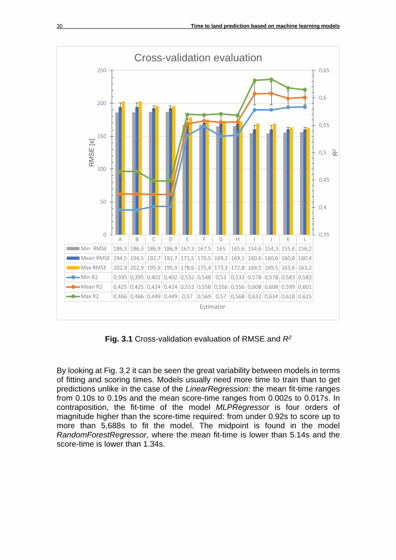
With this scheme, the estimator “A” is based in the LinearRegression model with the training set and the test set generated with the StratifiedShuffleSplit method and with a GridSearchCV as hyper-parameters tuner and so on and so forth. The following results have been obtained by running the cross_validate and cross_val_predict functions for each one of the pre-tuned estimators using the corresponding method: Fig. 3.1 shows how the mean RMSE drops from 194.5s (3 minutes and 14 seconds) with the estimator A to 160.4s (2 minutes and 40 seconds) with the estimator I while, with the same number of features, the mean R2 increases from 0.425 with the estimator A to 0.608 with the estimators I and J. Also, except for estimators E, F, G and H (MLPRegressor), the value of the R2 seems to follow a tendency towards reducing its variability in those cases where the split of the training set and the test set have been done by the method train_test_split (estimators C, D, K and L).
30 Time to land prediction based on machine learning models
Fig. 3.1 Cross-validation evaluation of RMSE and R2
By looking at Fig. 3.2 it can be seen the great variability between models in terms of fitting and scoring times. Models usually need more time to train than to get predictions unlike in the case of the LinearRegression: the mean fit-time ranges from 0.10s to 0.19s and the mean score-time ranges from 0.002s to 0.017s. In contraposition, the fit-time of the model MLPRegressor is four orders of magnitude higher than the score-time required: from under 0.92s to score up to more than 5,688s to fit the model. The midpoint is found in the model RandomForestRegressor, where the mean fit-time is lower than 5.14s and the score-time is lower than 1.34s.
A B C D E F G H I J K L
Min RMSE 186,3 186,3 186,9 186,9 167,3 167,5 165 165,6 154,6 154,3 155,6 156,2
Mean RMSE 194,5 194,5 192,7 192,7 171,5 170,5 169,2 169,1 160,6 160,6 160,8 160,4
Max RMSE 202,9 202,9 195,9 195,9 178,6 175,4 173,3 172,8 169,5 169,5 163,6 163,2
Min R2 0,395 0,395 0,402 0,402 0,532 0,548 0,53 0,533 0,578 0,578 0,583 0,583
Mean R2 0,425 0,425 0,424 0,424 0,553 0,558 0,556 0,556 0,608 0,608 0,599 0,601
Max R2 0,466 0,466 0,449 0,449 0,57 0,569 0,57 0,568 0,632 0,634 0,618 0,615
0,35
0,4
0,45
0,5
0,55
0,6
0,65
0
50
100
150
200
250
R2
RM
SE
[s]
Estimator
Cross-validation evaluation
RESULTS 31
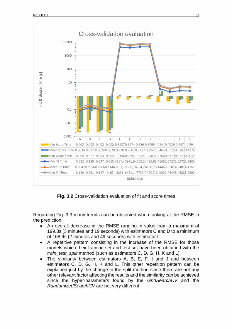
Fig. 3.2 Cross-validation evaluation of fit and score times
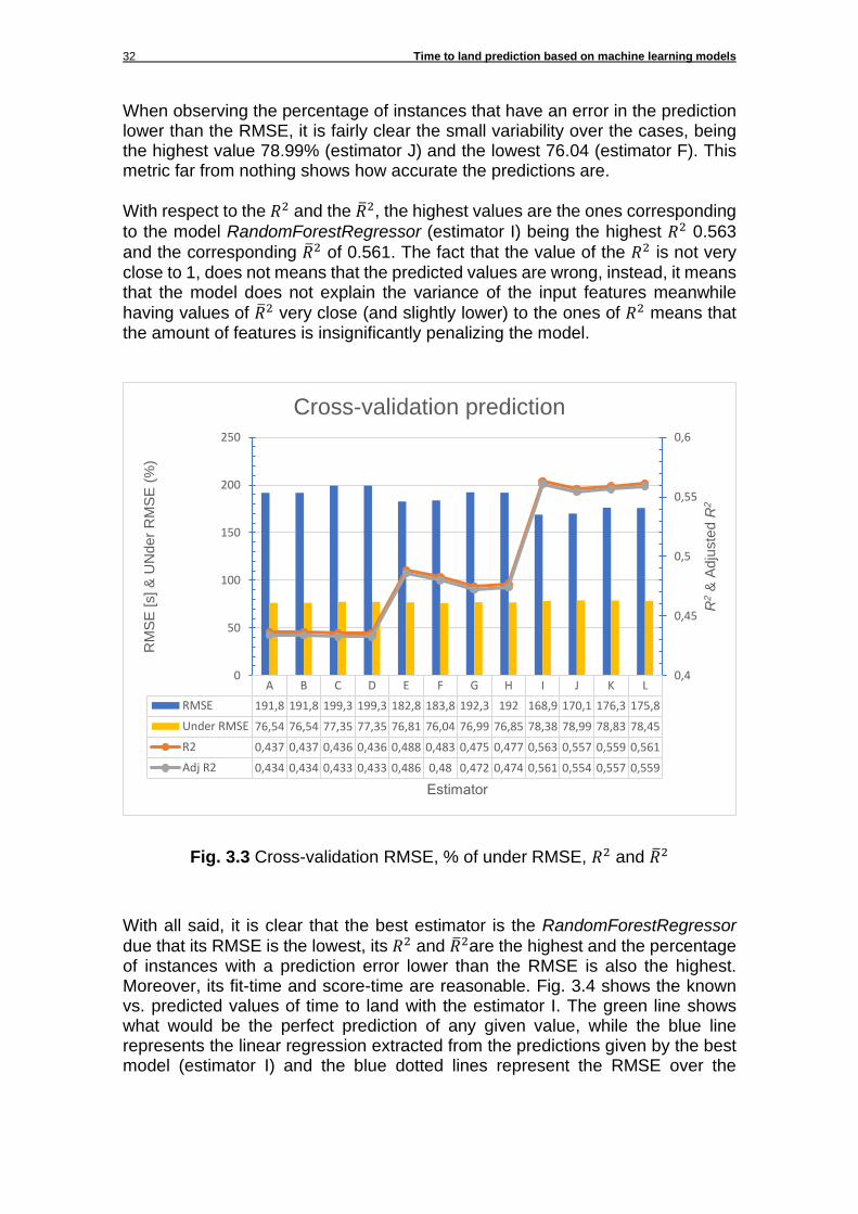
Regarding Fig. 3.3 many trends can be observed when looking at the RMSE in the prediction:
• An overall decrease in the RMSE ranging in value from a maximum of 199.3s (3 minutes and 19 seconds) with estimators C and D to a minimum of 168.9s (2 minutes and 49 seconds) with estimator I.
• A repetitive pattern consisting in the increase of the RMSE for those models which their training set and test set have been obtained with the train_test_split method (such as estimators C, D, G, H, K and L).
• The similarity between estimators A, B, E, F, I and J and between estimators C, D, G, H, K and L. This other repetition pattern can be explained just by the change in the split method since there are not any other relevant factor affecting the results and the similarity can be achieved since the hyper-parameters found by the GridSearchCV and the RandomizedSearchCV are not very different.
A B C D E F G H I J K L
Min Score Time 0,002 0,002 0,002 0,002 0,62870,5274 0,656 0,6095 0,34 0,4029 0,247 0,29
Mean Score Time 0,0034 0,017 0,00240,0028 0,928 0,76670,8727 0,894 1,34640,57250,52670,4179
Max Score Time 0,005 0,077 0,003 0,004 1,01980,92931,00241,21872,47660,62790,61290,5039
Min Fit Time 0,082 0,139 0,097 0,065 4357,43991,94559,24485,93,46652,07272,55762,3886
Mean Fit Time 0,10420,19560,10660,11487237,25688,16734,26190,75,14443,35014,84014,4761
Max Fit Time 0,139 0,261 0,127 0,15 8236 6481,1 7799 7429,7 6,406 3,74445,44825,0592
0,001
0,01
0,1
1
10
100
1000
10000F
it &
Score
TIm
e [s]
Estimator
Cross-validation evaluation
32 Time to land prediction based on machine learning models
When observing the percentage of instances that have an error in the prediction lower than the RMSE, it is fairly clear the small variability over the cases, being the highest value 78.99% (estimator J) and the lowest 76.04 (estimator F). This metric far from nothing shows how accurate the predictions are.
With respect to the 𝑅2 and the �̅�2, the highest values are the ones corresponding
to the model RandomForestRegressor (estimator I) being the highest 𝑅2 0.563
and the corresponding �̅�2 of 0.561. The fact that the value of the 𝑅2 is not very close to 1, does not means that the predicted values are wrong, instead, it means that the model does not explain the variance of the input features meanwhile
having values of �̅�2 very close (and slightly lower) to the ones of 𝑅2 means that the amount of features is insignificantly penalizing the model.
Fig. 3.3 Cross-validation RMSE, % of under RMSE, 𝑅2 and �̅�2
With all said, it is clear that the best estimator is the RandomForestRegressor
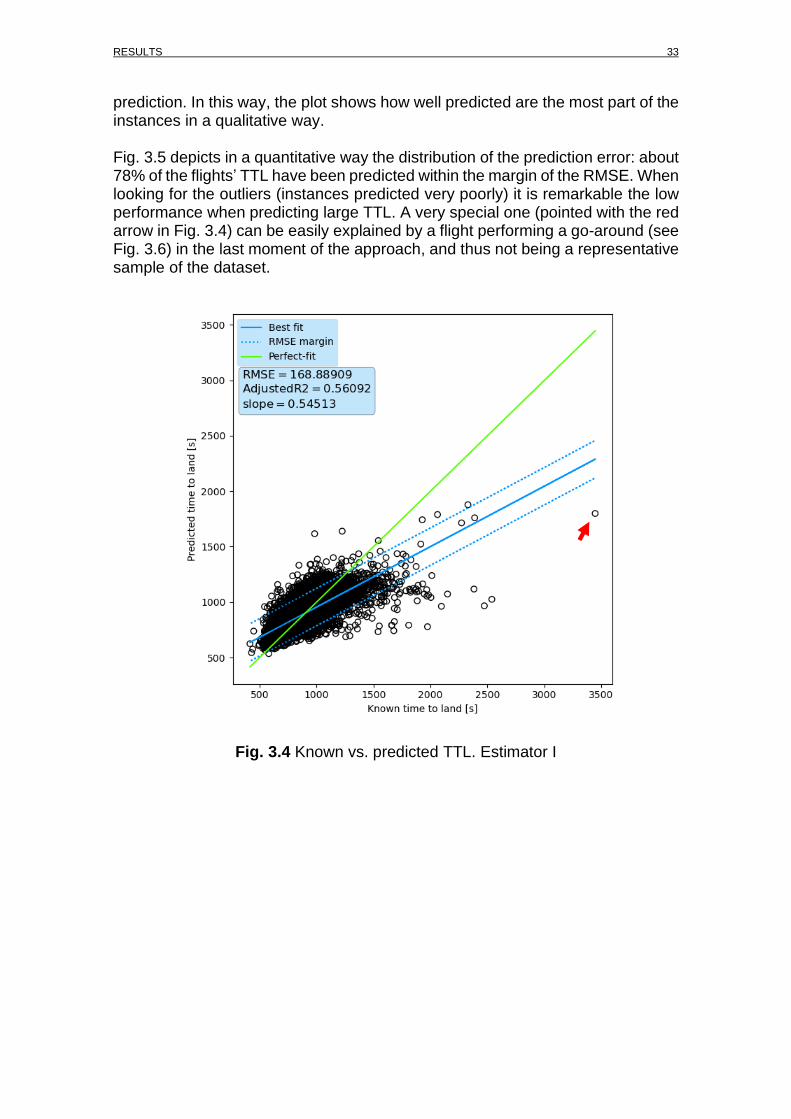
due that its RMSE is the lowest, its 𝑅2 and �̅�2are the highest and the percentage of instances with a prediction error lower than the RMSE is also the highest. Moreover, its fit-time and score-time are reasonable. Fig. 3.4 shows the known vs. predicted values of time to land with the estimator I. The green line shows what would be the perfect prediction of any given value, while the blue line represents the linear regression extracted from the predictions given by the best model (estimator I) and the blue dotted lines represent the RMSE over the
A B C D E F G H I J K L
RMSE 191,8 191,8 199,3 199,3 182,8 183,8 192,3 192 168,9 170,1 176,3 175,8
Under RMSE 76,54 76,54 77,35 77,35 76,81 76,04 76,99 76,85 78,38 78,99 78,83 78,45
R2 0,437 0,437 0,436 0,436 0,488 0,483 0,475 0,477 0,563 0,557 0,559 0,561
Adj R2 0,434 0,434 0,433 0,433 0,486 0,48 0,472 0,474 0,561 0,554 0,557 0,559
0,4
0,45
0,5
0,55
0,6
0
50
100
150
200
250
R2
& A
dju
ste
d R
2
RM
SE
[s] &
UN
der
RM
SE
(%
)
Estimator
Cross-validation prediction
RESULTS 33
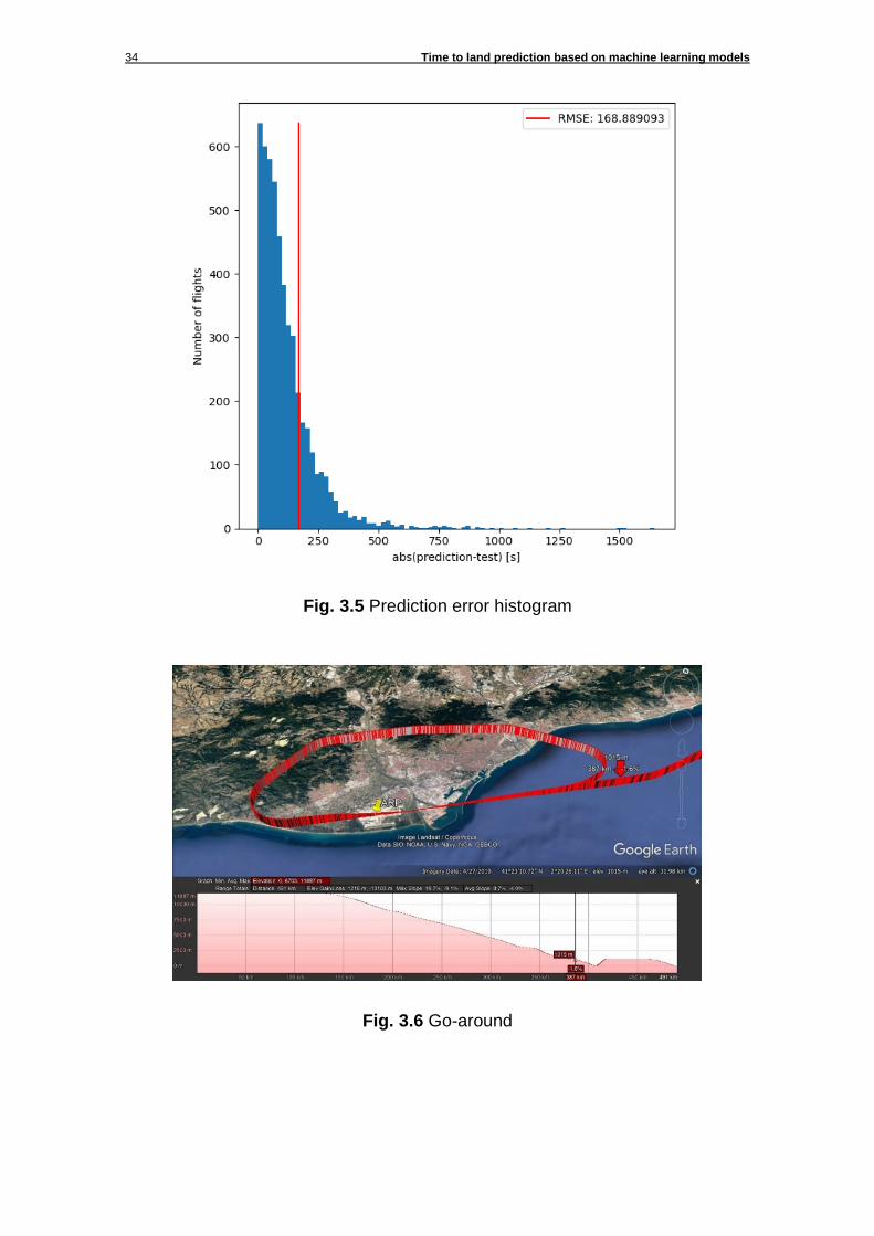
prediction. In this way, the plot shows how well predicted are the most part of the instances in a qualitative way. Fig. 3.5 depicts in a quantitative way the distribution of the prediction error: about 78% of the flights’ TTL have been predicted within the margin of the RMSE. When looking for the outliers (instances predicted very poorly) it is remarkable the low performance when predicting large TTL. A very special one (pointed with the red arrow in Fig. 3.4) can be easily explained by a flight performing a go-around (see Fig. 3.6) in the last moment of the approach, and thus not being a representative sample of the dataset.
Fig. 3.4 Known vs. predicted TTL. Estimator I
34 Time to land prediction based on machine learning models
Fig. 3.5 Prediction error histogram
Fig. 3.6 Go-around

CONCLUSIONS 35
CHAPTER 4. CONCLUSIONS After the realization of the project, it is necessary to recapitulate and extract all the conclusions related to the initial objective: predict the time any aircraft would take to land in Josep Tarradellas Barcelona-El Prat Airport. In the one hand, it has been proven the feasibility of predicting the amount of time required to land from a certain distance, to the chosen airport. Following the mentioned methodology, the most precise and accurate model has been the RandomForestRegressor with the lowest values of RMSE and the highest 𝑅2 and
�̅�2 while keeping the most part of predictions within the RMSE margin. More specifically, from the four variants of the same model, the best is that with the training and test models split using the stratified shuffle split function and with the hyper-parameters tuned found with the exhaustive search using the GridSearchCV method. Although not being the fastest model in terms of fitting and scoring, it offers the best combinations of both: the fit-time is slightly larger than the score-time so it is more convenient to be implemented in a real environment. In the other hand, because of the computational power needed to execute some ML algorithms given its combinational nature, the existence of a solution with better predictions is feasible. Although, considering the limited resources of this project and its reasonable results, it is hopeful start which can lead to new projects. Another aspect to get better results would be the inclusion of more data in the dataset to minimise the effect of outliers (produced by go-arounds, for example). Also, the input data could be widen by the inclusion of more effective range of ADS-B coverage by using reports received from nearby ADS-B antennas as it is done with the flightradar24 network.

36 Time to land prediction based on machine learning models
Bibliography
[1] Wikipedia, “Search tree,” [Online]. Available: https://en.wikipedia.org/wiki/Search_tree.
[2] Wikipedia, “Minimax,” [Online]. Available: https://en.wikipedia.org/wiki/Minimax.
[3] SESAR, “INTERACTIVE TOOLSET FOR UNDERSTANDING TRADE-OFFS IN ATM PERFORMANCE - INTUIT,” [Online]. Available: https://www.sesarju.eu/projects/intuit.
[4] SESAR, “COPTRA,” [Online]. Available: https://www.sesarju.eu/projects/coptra.
[5] BigData4ATM, “BigData4ATM,” [Online]. Available: https://www.bigdata4atm.eu/.
[6] SESAR, “MALORCA: Improving ATM efficiency through artificial intelligence,” [Online]. Available: https://www.sesarju.eu/projects/malorca.
[7] SESAR Joint Undertaking, “Modern ATM via Human/Automation Learning Optimisation,” [Online]. Available: https://cordis.europa.eu/project/id/892970.
[8] Wikipedia, “Ordinary Least Squares,” [Online]. Available: https://en.wikipedia.org/wiki/Ordinary_least_squares.
[9] Wikipedia, “Multi-layer perceptron,” [Online]. Available: https://en.wikipedia.org/wiki/Multilayer_perceptron.
[10] Wikipedia, “Random Forest Regressor,” [Online]. Available: https://en.wikipedia.org/wiki/Random_forest.
[11] Scikit-learn, “StratifiedKFold,” [Online]. Available: https://scikit-learn.org/stable/modules/generated/sklearn.model_selection.StratifiedKFold.html.
[12] Scikit-learn, “ShuffleSplit,” [Online]. Available: https://scikit-learn.org/stable/modules/generated/sklearn.model_selection.ShuffleSplit.html.
[13] Wikipedia, “R2,” [Online]. Available: https://en.wikipedia.org/wiki/Coefficient_of_determination.
[14] Aena, “Estadísticas de tráfico aereo. Informes mensuales,” [Online]. Available: http://www.aena.es/csee/ccurl/131/368/3.Estadisticas_Marzo_2020%20(1).pdf.
[15] M. P. Batlle, “ADS-B Decoder”.
[16] Wikipedia, “ICAO 24-bit address,” [Online]. Available: https://en.wikipedia.org/wiki/Aviation_transponder_interrogation_modes#ICAO_24-bit_address.
[17] SKYbrary, “4D trajectory Concept,” [Online]. Available: https://www.skybrary.aero/index.php/4D_Trajectory_Concept?utm_source=SKYbrary&utm_campaign=b60834be85-SKYbrary_Highlight_06_01_2014&utm_medium=email&utm_term=0_e405169b04-b60834be85-264059017.

Bibliography 37
[18] The LPA Group, “Airfield Demand/Capacity Analysis & Facility Requirements,” [Online]. Available: https://www.flyjacksonville.com/PDFs/HegMP/HEGChapterRequirements(05-12-08).pdf.
[19] Wikipedia, “Wake turbulence,” [Online]. Available: https://en.wikipedia.org/wiki/Wake_turbulence.
[20] Wikipedia, “Web scraping,” [Online]. Available: https://en.wikipedia.org/wiki/Web_scraping.
[21] Scikit-learn, “Pipeline,” [Online]. Available: https://scikit-learn.org/stable/modules/generated/sklearn.pipeline.Pipeline.html.
[22] Scikit-learn, “SimpleImputer,” [Online]. Available: https://scikit-learn.org/stable/modules/generated/sklearn.impute.SimpleImputer.html.
[23] Scikit-learn, “MinMaxScaler,” [Online]. Available: https://scikit-learn.org/stable/modules/generated/sklearn.preprocessing.MinMaxScaler.html.
[24] Scikit-learn, “StandardScaler,” [Online]. Available: https://scikit-learn.org/stable/modules/generated/sklearn.preprocessing.StandardScaler.html.
[25] Scikit-learn, “LabelBinarizer,” [Online]. Available: https://scikit-learn.org/stable/modules/generated/sklearn.preprocessing.LabelBinarizer.html.
[26] ICAO, “Doc. 8643. Part 2 - Aircraft type designators (decode)”.
[27] J. Sun, “The 1090MHz Riddle,” 2017. [Online]. Available: https://mode-s.org/decode/book-the_1090mhz_riddle-junzi_sun.pdf.
[28] Wikipedia, “Root-mean-square deviation,” [Online]. Available: https://en.wikipedia.org/wiki/Root-mean-square_deviation.
[29] Scikit-learn, “Scikit-learn: Machine Learning in Python, Pedregosa et al., JMLR 12, pp. 2825-2830, 2011.”.
[30] S. Raschka, “Scale training test,” [Online]. Available: https://sebastianraschka.com/faq/docs/scale-training-test.html.
[31] N. E. Helwig, “Multiple Linear Regression,” [Online]. Available: http://users.stat.umn.edu/~helwig/notes/mvlr-Notes.pdf.