Embed Size (px)
Citation preview
Treball Final de Grau
Tutor
Dra. Anna de Juan Capdevila Departamento de Química Analítica
Design and application of chemometric methods to the determination of compounds of interest in biodiesels.
Diseño y aplicación de métodos quimiométricos para la determinación de compuestos de interés en biodiésel.
Rodrigo Rocha de Oliveira June 2013


Aquesta obra esta subjecta a la llicència de: Reconeixement–NoComercial-SenseObraDerivada
http://creativecommons.org/licenses/by-nc-nd/3.0/es/


To my parents, Maria Dalva Rocha de Oliveira and
Raimundo Gregório de Oliveira. For the love, education and effort
given to me.
Acknowledgements
I would like to thank Dr. Anna de Juan and Dr. Kássio Lima for the opportunity to
develop this work and the rich knowledge transmitted.
I would also like to thank my friends from the Chemometrics groups (UFRN and UB)
and the friends that I knew through this journey in this wonderful city.
I’m very thankful to the financial support provided by the Brazilian government through
the exchange grant and the laboratories LCL (UFRN) and Lamoc (Inmetro).
Finally, I would like to thank my beloved family for always gave me strength and
support to rise in this life. And to my kind girlfriend for her patience and understanding.
What I cannot create, I do not understand
Richard Feynman.

REPORT

Design and application of chemometric methods to the determination of compounds of interest in biodiesels. 1
CONTENTS
SUMMARY 3
RESUMEN 5
1. INTRODUCTION 7
1.1. BIODIESEL 7
1.2. CHEMOMETRICS 9
1.3. SPECTROSCOPIC APPLICATIONS IN BIODIESEL ANALYSIS 10
2. EXPERIMENTAL 11
2.1. RAW MATERIALS AND SAMPLE PREPARATION 11
2.2. INSTRUMENTATION AND EXPERIMENTAL MEASUREMENTS 12
3. DATA TREATMENT 13
3.1. DATASETS 13
3.2. CHEMOMETRIC METHODS 15
3.2.1. Partial least squares (PLS) regression 15
3.2.2. Multivariate curve resolution alternating least squares (MCR-ALS) 17
3.2.2.1. Correlation constraint 19
3.2.3. Figures of merit 22
3.2.4. Chemometric software 23
4. RESULTS AND DISCUSSION 25
4.1. ANALYSIS OF DIESEL AND BIODIESEL BLENDS 25
4.2. ANALYSIS OF BIODIESELS AND ANTIOXIDANT MIXTURES 29
CONCLUSIONS 33
REFERENCES 35
APPENDICES 39
APPENDIX 1. MAIN MCR-ALS FUNCTION 41

2 Rocha de Oliveira, Rodrigo
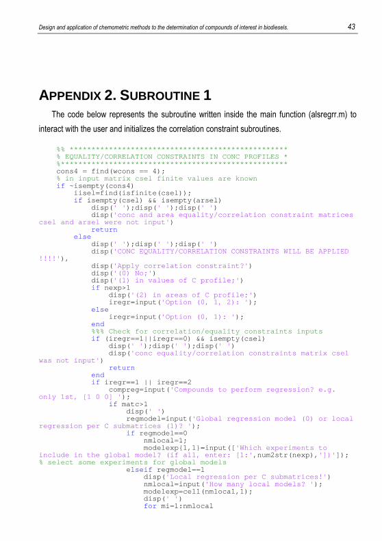
APPENDIX 2. SUBROUTINE 1 43
APPENDIX 3. SUBROUTINE 2 45
APPENDIX 4. CORRELATION CONSTRAINT FUNCTION 47
APPENDIX 5. COMPACT DISC 49
Design and application of chemometric methods to the determination of compounds of interest in biodiesels. 3
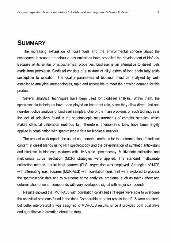
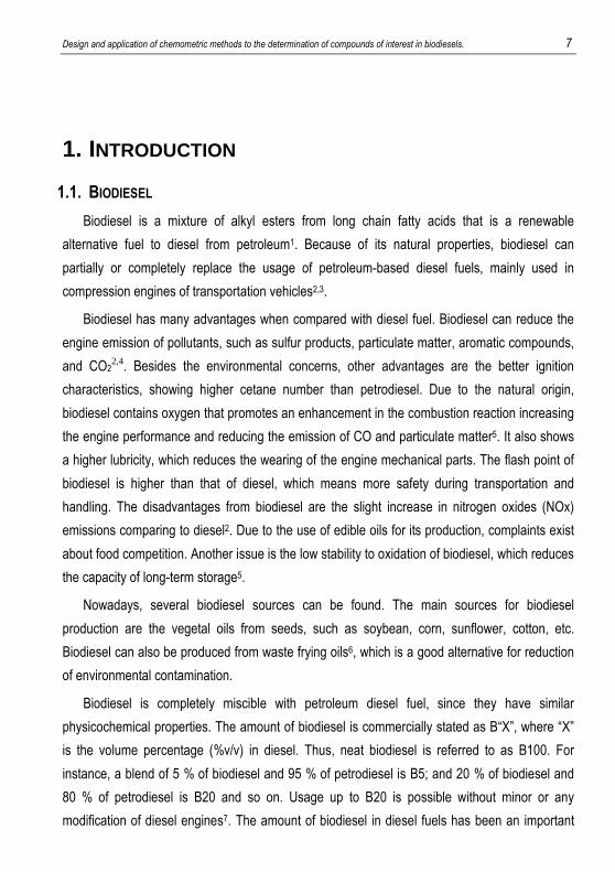
SUMMARY The increasing exhaustion of fossil fuels and the environmental concern about the
consequent increased greenhouse gas emissions have propelled the development of biofuels.
Because of its similar physicochemical properties, biodiesel is an alternative to diesel fuels
made from petroleum. Biodiesel consists of a mixture of alkyl esters of long chain fatty acids
susceptible to oxidation. The quality parameters of biodiesel must be analyzed by well-
established analytical methodologies, rapid and accessible to meet the growing demand for this
product.
Several analytical techniques have been used for biodiesel analysis. Within them, the
spectroscopic techniques have been played an important role, since they allow direct, fast and
non-destructive analysis of biodiesel samples. One of the main problems of such techniques is
the lack of selectivity found in the spectroscopic measurements of complex samples, which
makes classical calibration methods fail. Therefore, chemometric tools have been largely
applied in combination with spectroscopic data for biodiesel analysis.
The present work reports the use of chemometric methods for the determination of biodiesel
content in diesel blends using NIR spectroscopy and the determination of synthetic antioxidant
and biodiesel in biodiesel mixtures with UV-Visible spectroscopy. Multivariate calibration and
multivariate curve resolution (MCR) strategies were applied. The standard multivariate
calibration method, partial least squares (PLS) regression was employed. Strategies of MCR
with alternating least squares (MCR-ALS) with correlation constraint were explored to process
the spectroscopic data and to overcome some analytical problems, such as matrix effect and
determination of minor compounds with very overlapped signal with major compounds.
Results showed that MCR-ALS with correlation constraint strategies were able to overcome
the analytical problems found in the data. Comparable or better results than PLS were obtained,
but better interpretability was assigned to MCR-ALS results, since it provided both qualitative
and quantitative information about the data.

Design and application of chemometric methods to the determination of compounds of interest in biodiesels. 5
RESUMEN El creciente aumento del consumo de combustibles fósiles y la preocupación por el
consiguiente aumento de la emisión de gases de efecto invernadero han promovido el
desarrollo de biocombustibles. El biodiésel es una alternativa para el diésel de petróleo debido
a sus semejantes propiedades físico-químicas. El biodiésel consta de una mezcla de ésteres
alquílicos de ácidos grasos de cadena larga susceptibles a oxidación. Los parámetros de
calidad de biodiésel deben ser analizados por metodologías analíticas robustas, rápidas y
asequibles para cubrir la demanda creciente del producto.
Diversas técnicas analíticas han sido utilizadas para el análisis de biodiésel. Dentro de las
cuales, las técnicas espectroscópicas han tenido un papel muy importante, ya que permiten un
análisis de biodiésel directo, rápido y no destructivo. Uno de los principales problemas de estas
técnicas es la falta de selectividad en la señal asociada a muestras complejas, lo cual hace que
los métodos de calibración clásicos fracasen. Por eso, son necesarias herramientas
quimiométricas en combinación con datos espectroscópicos para el análisis de biodiésel.
El presente trabajo presenta el uso de métodos quimiométricos para la determinación de
biodiésel en mezclas con diésel utilizando espectroscopia NIR y para la determinación de
antioxidante y biodiésel en mezclas de biodiésel utilizando espectroscopia UV-Visible. Se han
empleado calibración multivariante y estrategias de resolución multivariante de curvas (MCR).
Se ha empleado el método de calibración multivariante estándar, la regresión por el método de
los mínimos cuadrados parciales (PLS). También se han utilizado estrategias MCR por
mínimos cuadrados alternados (MCR-ALS) y la restricción de correlación para procesar los
datos espectroscópicos y superar problemas analíticos, como el efecto de matriz y la
determinación de compuestos minoritarios con una señal muy solapada con la de compuestos
mayoritarios.
Los resultados indican que MCR-ALS con estrategias de restricción de correlación fue
capaz de resolver los problemas mencionados anteriormente. Se obtuvieron resultados
comparables o mejores que con el método PLS. Sin embargo, los resultados obtenidos con

6 Rocha de Oliveira, Rodrigo
MCR-ALS tienen una mayor interpretabilidad, porque este método proporciona información
cualitativa y cuantitativa acerca de los datos.
Design and application of chemometric methods to the determination of compounds of interest in biodiesels. 7
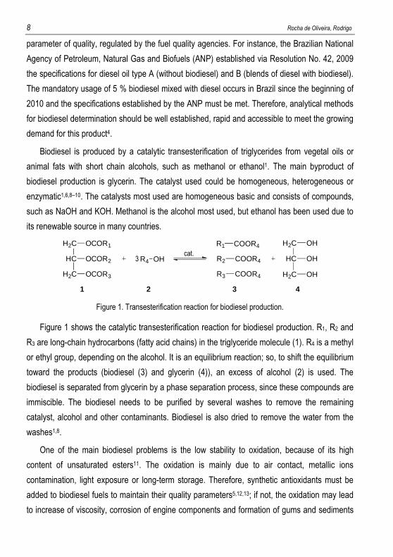
1. INTRODUCTION
1.1. BIODIESEL
Biodiesel is a mixture of alkyl esters from long chain fatty acids that is a renewable
alternative fuel to diesel from petroleum1. Because of its natural properties, biodiesel can
partially or completely replace the usage of petroleum-based diesel fuels, mainly used in
compression engines of transportation vehicles2,3.
Biodiesel has many advantages when compared with diesel fuel. Biodiesel can reduce the
engine emission of pollutants, such as sulfur products, particulate matter, aromatic compounds,
and CO22,4. Besides the environmental concerns, other advantages are the better ignition
characteristics, showing higher cetane number than petrodiesel. Due to the natural origin,
biodiesel contains oxygen that promotes an enhancement in the combustion reaction increasing
the engine performance and reducing the emission of CO and particulate matter5. It also shows
a higher lubricity, which reduces the wearing of the engine mechanical parts. The flash point of
biodiesel is higher than that of diesel, which means more safety during transportation and
handling. The disadvantages from biodiesel are the slight increase in nitrogen oxides (NOx)
emissions comparing to diesel2. Due to the use of edible oils for its production, complaints exist
about food competition. Another issue is the low stability to oxidation of biodiesel, which reduces
the capacity of long-term storage5.
Nowadays, several biodiesel sources can be found. The main sources for biodiesel
production are the vegetal oils from seeds, such as soybean, corn, sunflower, cotton, etc.
Biodiesel can also be produced from waste frying oils6, which is a good alternative for reduction
of environmental contamination.
Biodiesel is completely miscible with petroleum diesel fuel, since they have similar
physicochemical properties. The amount of biodiesel is commercially stated as B“X”, where “X”
is the volume percentage (%v/v) in diesel. Thus, neat biodiesel is referred to as B100. For
instance, a blend of 5 % of biodiesel and 95 % of petrodiesel is B5; and 20 % of biodiesel and
80 % of petrodiesel is B20 and so on. Usage up to B20 is possible without minor or any
modification of diesel engines7. The amount of biodiesel in diesel fuels has been an important
8 Rocha de Oliveira, Rodrigo
parameter of quality, regulated by the fuel quality agencies. For instance, the Brazilian National
Agency of Petroleum, Natural Gas and Biofuels (ANP) established via Resolution No. 42, 2009
the specifications for diesel oil type A (without biodiesel) and B (blends of diesel with biodiesel).
The mandatory usage of 5 % biodiesel mixed with diesel occurs in Brazil since the beginning of
2010 and the specifications established by the ANP must be met. Therefore, analytical methods
for biodiesel determination should be well established, rapid and accessible to meet the growing
demand for this product4.
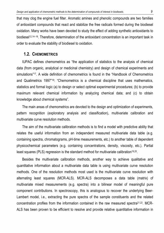
Biodiesel is produced by a catalytic transesterification of triglycerides from vegetal oils or
animal fats with short chain alcohols, such as methanol or ethanol1. The main byproduct of
biodiesel production is glycerin. The catalyst used could be homogeneous, heterogeneous or
enzymatic1,6,8–10. The catalysts most used are homogeneous basic and consists of compounds,
such as NaOH and KOH. Methanol is the alcohol most used, but ethanol has been used due to
its renewable source in many countries.
Figure 1. Transesterification reaction for biodiesel production.
Figure 1 shows the catalytic transesterification reaction for biodiesel production. R1, R2 and
R3 are long-chain hydrocarbons (fatty acid chains) in the triglyceride molecule (1). R4 is a methyl
or ethyl group, depending on the alcohol. It is an equilibrium reaction; so, to shift the equilibrium
toward the products (biodiesel (3) and glycerin (4)), an excess of alcohol (2) is used. The
biodiesel is separated from glycerin by a phase separation process, since these compounds are
immiscible. The biodiesel needs to be purified by several washes to remove the remaining
catalyst, alcohol and other contaminants. Biodiesel is also dried to remove the water from the
washes1,8.
One of the main biodiesel problems is the low stability to oxidation, because of its high
content of unsaturated esters11. The oxidation is mainly due to air contact, metallic ions
contamination, light exposure or long-term storage. Therefore, synthetic antioxidants must be
added to biodiesel fuels to maintain their quality parameters5,12,13; if not, the oxidation may lead
to increase of viscosity, corrosion of engine components and formation of gums and sediments
H2C
HC
H2C
OCOR1
OCOR2
OCOR3
R4 OH
H2C
HC
H2C
OH
OH
OH
R1 COOR4
R2 COOR4
R3 COOR4
3cat.
1 2 3 4
Design and application of chemometric methods to the determination of compounds of interest in biodiesels. 9
that may clog the engine fuel filter. Aromatic amines and phenolic compounds are two families
of antioxidant compounds that react and stabilize the free radicals formed during the biodiesel
oxidation. Many works have been devoted to study the effect of adding synthetic antioxidants to
biodiesel12,14–16. Therefore, determination of the antioxidant concentration is an important task in
order to evaluate the stability of biodiesel to oxidation.
1.2. CHEMOMETRICS
IUPAC defines chemometrics as “the application of statistics to the analysis of chemical
data (from organic, analytical or medicinal chemistry) and design of chemical experiments and
simulations”17. A wide definition of chemometrics is found in the “Handbook of Chemometrics
and Qualimetrics 1997”18: “Chemometrics is a chemical discipline that uses mathematics,
statistics and formal logic (a) to design or select optimal experimental procedures; (b) to provide
maximum relevant chemical information by analyzing chemical data; and (c) to obtain
knowledge about chemical systems”.
The main areas of chemometrics are devoted to the design and optimization of experiments,
pattern recognition (exploratory analysis and classification), multivariate calibration and
multivariate curve resolution methods.
The aim of the multivariate calibration methods is to find a model with predictive ability that
relates the useful information from an independent measured multivariate data table (e.g.
containing spectra, chromatograms, pH-time measurements, etc.) to another table of dependent
physicochemical parameters (e.g. containing concentrations, density, viscosity, etc.). Partial
least squares (PLS) regression is the standard method for multivariate calibration19,20.
Besides the multivariate calibration methods, another way to achieve qualitative and
quantitative information about a multivariate data table is using multivariate curve resolution
methods. One of the resolution methods most used is the multivariate curve resolution with
alternating least squares (MCR-ALS). MCR-ALS decomposes a data table (matrix) of
multivariate mixed measurements (e.g. spectra) into a bilinear model of meaningful pure
component contributions. In spectroscopy, this is analogous to recover the underlying Beer-
Lambert model, i.e., extracting the pure spectra of the sample constituents and the related
concentration profiles from the information contained in the raw measured spectra21,22. MCR-
ALS has been proven to be efficient to resolve and provide relative quantitative information in
10 Rocha de Oliveira, Rodrigo
different types of complex processes and mixtures21, such as liquid chromatography with diode
array detection23–25 and spectral data from industrial processes26,27.
Detailed explanation about PLS and MCR-ALS methods and the suitable multivariate data
structures are provided in section 3.
1.3. SPECTROSCOPIC AND CHEMOMETRICS APPLICATIONS IN BIODIESEL
Spectroscopic techniques have been applied for the determination of several parameters in
biodiesel. All the spectroscopic range from ultraviolet to mid infrared absorption spectroscopy
has been used in many works for determination of biodiesel parameters from different
sources28–37, as well as molecular fluorescence spectroscopy38,39. Biodiesel analysis with
infrared spectroscopy has been the subject of many works, due to the direct, reliable, fast and
non-destructive sample analysis29,33. Spectroscopic measurements suffer for the lack of
selectivity when complex samples are analyzed, since the signal are very overlapped which
makes classical calibration methods fail. Thus, analytical techniques, such as near infrared
(NIR) spectroscopy need the use of chemometrics tools to solve these analytical problems.
Several chemometric methods have been applied to spectroscopic biodiesel analysis.
Linear multivariate calibration methods, such as multivariate linear regression (MLR), principal
component regression, partial least squares (PLS) regression, and non-linear methods, such as
support vector machines (SVM) and artificial neural networks (ANN) have been often used to
extract information from NIR spectra for determination of quality parameters in biodiesel and
biodiesel/diesel blends29,32,34–36. Chemometric methods for classification, such as soft
independent modeling of class analogy (SIMCA), hierarchical cluster analysis (HCA),
successive projections algorithm with linear discriminant analysis (SPA-LDA) and PLS
discriminant analysis (PLS-DA) have been used to classify biodiesel according to the production
source37–39. Variable selection methods, such as Genetic Algorithm, interval-PLS, SPA and
others, have been used to reduce the number of used spectral variables and improve the
abilities of calibration and classification models29,32,39,40.
Different analytical methodologies were proposed for biodiesel antioxidant analysis. Tormin
et. al. developed methods based on the amperometric determination of tert-
butylhydroquinone41, butylated hydroxyanisole42 and mixtures of the two compounds by batch-
injection analysis43 in synthetic samples of biodiesel. The aromatic amine N,N’-Di-sec-butyl-p-
phenylenediamine (PDA) has been proven to be an efficient antioxidant and a versatile artificial
Design and application of chemometric methods to the determination of compounds of interest in biodiesels. 11
marker for biodiesel and has been analyzed by easy ambient sonic-spray ionization mass
spectrometry44. Peaks in the mid infrared region were also used for calibration and
determination of PDA antioxidant in sunflower biodiesel mixtures45.
MCR-ALS has been applied in a few works for biodiesel analysis. Only two works were
found, where MCR-ALS was used to resolve spectrophotometric sequential injection analysis
data in the determination of sulphate and acidity of biodiesel samples46,47.
2. EXPERIMENTAL
2.1. RAW MATERIALS AND SAMPLE PREPARATION
Two sets of samples were used in this work. The first set of samples contained mixtures of
neat diesel and soybean biodiesel provided by the Laboratory of Fuels and Lubricants (LCL) of
the Federal University of Rio Grande do Norte (UFRN), RN, Brazil. Biodiesel was prepared by
the basic catalyzed transesterification reaction of commercial soybean vegetal oil with methanol.
38 samples were prepared in two batches of 30 and 8 samples, respectively. The first batch
was prepared and submitted to natural aging for about three months before measurement. The
second batch was freshly prepared and measured. Percentage of biodiesel in samples was
determined following the European method EN 14078 and ranged from 0 to 20.5% (v/v).
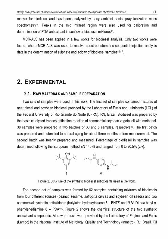
Figure 2. Structure of the synthetic biodiesel antioxidants used in the work.
The second set of samples was formed by 62 samples containing mixtures of biodiesels
from four different sources (peanut, sesame, Jatropha curcas and soybean oil seeds) and two
commercial synthetic antioxidants (butylated hydroxytoluene 5 – BHT48 and N,N’ -Di-sec-butyl-p-
phenylenediamine 6 – PDA49). Figure 2 shows the chemical structure of the two synthetic
antioxidant compounds. All raw products were provided by the Laboratory of Engines and Fuels
(Lamoc) in the National Institute of Metrology, Quality and Technology (Inmetro), RJ, Brazil. Oil
12 Rocha de Oliveira, Rodrigo
seed extraction and biodiesel synthesis were carried out by Lamoc following the method used
in45. A cubic D-optimal mixture design was developed with Design-Expert® (Stat-Ease Inc.,
Minneapolis, MN, USA) software to set the composition of the samples. All samples were
prepared according to the required composition for a total sample mass of 4 g. The
concentration of antioxidants covered the range commercially used for biodiesel fuels. To
achieve low concentration levels for antioxidants, diluted stock solutions of each antioxidant
were prepared using each biodiesel as solvent. The range of concentrations for each compound
is described in Table 1.
Table 1 Experimental concentration statistics for the six components in the 62 mixture samples.
Kind of biodiesel [% w/w] Antioxidant [ppm]
PNa SEb JCc SBd BHTe PDAf
Min. 0.18 0.19 0.18 0.18 2 1
Max. 99.38 99.30 99.39 53 2632 1006
Mean 24.42 26.12 23.56 22.33 892 302
Std. 18.07 19.71 19.23 15.01 712 232 (a) PN: peanut. (b) SE: sesame. (c) JC: Jatropha curcas. (d) SB: soybean. (e) BHT: butylated hydroxytoluene. (f) PDA: N,N’-Di-sec-butyl-p-phenylenediamine.
2.2. INSTRUMENTATION AND EXPERIMENTAL MEASUREMENTS
Near infrared spectra of biodiesel blends were recorded using a FT-NIR spectrophotometer
model MB 160 (Bomem). Spectra were collected in cells with two optical pathlengths: 10 mm
(for the spectral range between 1105 – 1677 nm) and 1.0 mm (for the spectral range between
2111 – 3216 nm) to compensate the different signal intensity in the two spectral ranges
acquired.
UV-Visible spectra of biodiesel and antioxidant mixtures were acquired with a UV-Visible
spectrophotometer model Evolution 60S (Thermo Scientific) in the spectral range 370 – 670 nm,
with a wavelength increment of 2 nm among consecutive measurements. A 10 mm pathlength
quartz cuvette was used.
Pure compound NIR and UV-Visible spectrum were also recorded to be used afterwards in
the chemometric analysis.
Design and application of chemometric methods to the determination of compounds of interest in biodiesels. 13
3. DATA TREATMENT
3.1. DATASETS
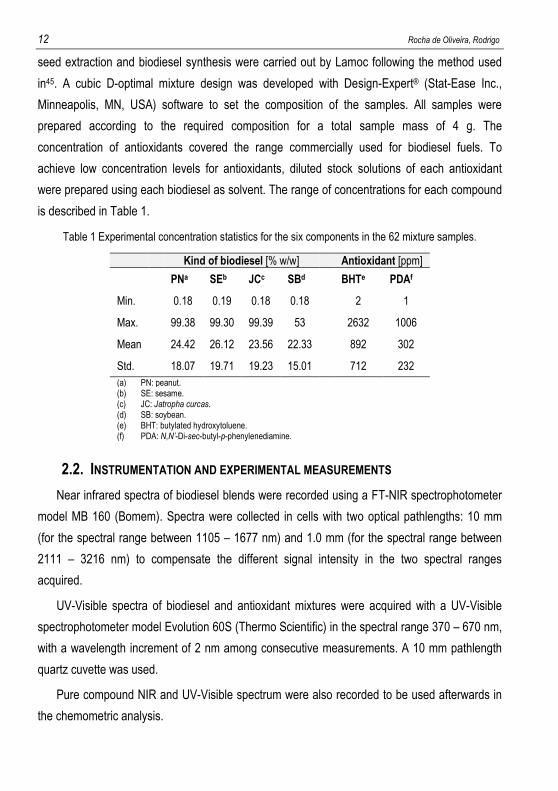
A dataset matrix formed by multivariate data is usually designed as a matrix � of size �� � ��, where � is the number of rows that represent the different samples and � is the number
of columns that, in this case, are the wavelengths of the acquired spectra. Figure 3 shows the
representation of a multivariate data matrix �, where ���,� means the absorbance of sample � at wavelength �.
Figure 3. Structure representation of a multivariate data matrix.
The first set of samples, which contained the blends of biodiesel and diesel, gave a data
matrix formed by the NIR spectra collected. Two samples were removed as spectral outliers
from the first batch; thus, the final size of the matrix was �36 � 1224� , with the rows
containing the samples spectra and the columns designing the wavelength variables. The first
28 spectra were from the first aged batch and the last 8 from the second fresh batch. The first
801 columns were associated with the spectral range (1105 – 1677 nm), referred to spectra
collected with the 10 mm pathlength cell, and the last 423 columns covered the range (2111 –
3216 nm), used in the spectra recorded with the 1.0 mm pathlength cell. Figure 4a shows the
original NIR spectra covering the two spectral ranges used. The spectral preprocessing
methods applied were the offset correction to remove negative values in the spectra, followed
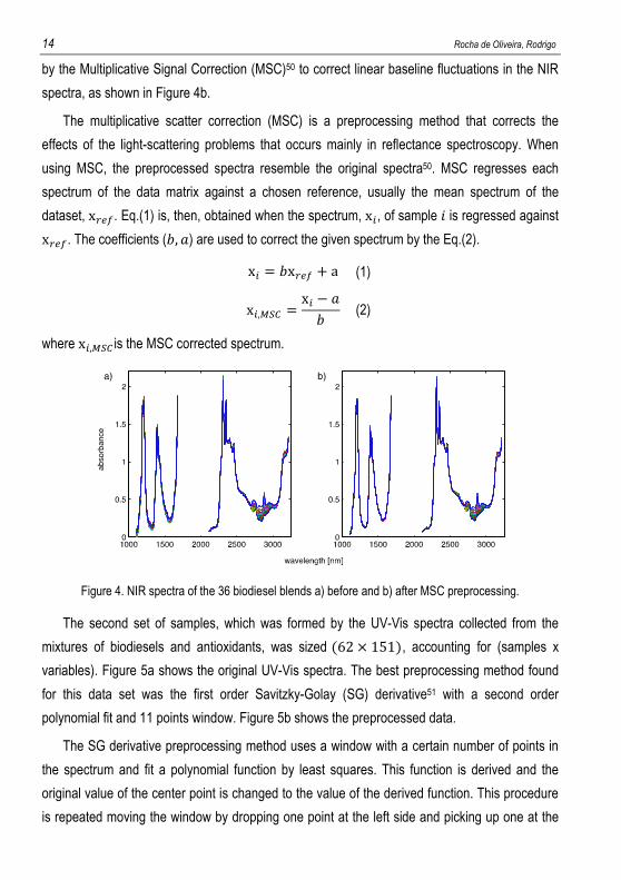
14 Rocha de Oliveira, Rodrigo
by the Multiplicative Signal Correction (MSC)50 to correct linear baseline fluctuations in the NIR
spectra, as shown in Figure 4b.
The multiplicative scatter correction (MSC) is a preprocessing method that corrects the
effects of the light-scattering problems that occurs mainly in reflectance spectroscopy. When
using MSC, the preprocessed spectra resemble the original spectra50. MSC regresses each
spectrum of the data matrix against a chosen reference, usually the mean spectrum of the
dataset, x���. Eq.(1) is, then, obtained when the spectrum, x�, of sample � is regressed against x���. The coefficients (�, �) are used to correct the given spectrum by the Eq.(2).
x� = �x��� + a (1)
x�,��� = x� − �� (2)
where x�,��� is the MSC corrected spectrum.
Figure 4. NIR spectra of the 36 biodiesel blends a) before and b) after MSC preprocessing.
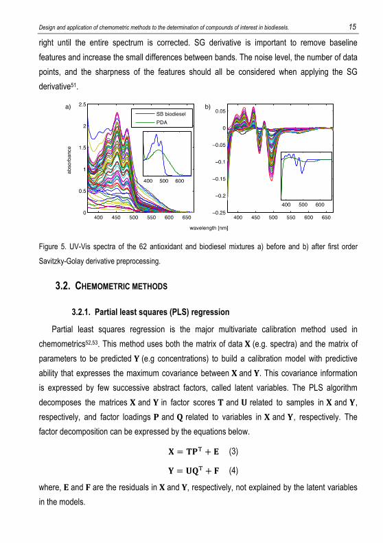
The second set of samples, which was formed by the UV-Vis spectra collected from the
mixtures of biodiesels and antioxidants, was sized (62 × 151), accounting for (samples x
variables). Figure 5a shows the original UV-Vis spectra. The best preprocessing method found
for this data set was the first order Savitzky-Golay (SG) derivative51 with a second order
polynomial fit and 11 points window. Figure 5b shows the preprocessed data.
The SG derivative preprocessing method uses a window with a certain number of points in
the spectrum and fit a polynomial function by least squares. This function is derived and the
original value of the center point is changed to the value of the derived function. This procedure
is repeated moving the window by dropping one point at the left side and picking up one at the
Design and application of chemometric methods to the determination of compounds of interest in biodiesels. 15
right until the entire spectrum is corrected. SG derivative is important to remove baseline
features and increase the small differences between bands. The noise level, the number of data
points, and the sharpness of the features should all be considered when applying the SG
derivative51.
Figure 5. UV-Vis spectra of the 62 antioxidant and biodiesel mixtures a) before and b) after first order
Savitzky-Golay derivative preprocessing.
3.2. CHEMOMETRIC METHODS
3.2.1. Partial least squares (PLS) regression
Partial least squares regression is the major multivariate calibration method used in
chemometrics52,53. This method uses both the matrix of data � (e.g. spectra) and the matrix of
parameters to be predicted � (e.g concentrations) to build a calibration model with predictive
ability that expresses the maximum covariance between � and �. This covariance information
is expressed by few successive abstract factors, called latent variables. The PLS algorithm
decomposes the matrices � and � in factor scores and ! related to samples in � and �,
respectively, and factor loadings " and # related to variables in � and �, respectively. The
factor decomposition can be expressed by the equations below.
� = "$ + % (3)
� = !#$ + & (4)
where, % and & are the residuals in � and �, respectively, not explained by the latent variables
in the models.
16 Rocha de Oliveira, Rodrigo
The regression model is obtained by the Eq.(5) using and !.
! = '"() (5)
where '"() is the vector of regression coefficients.
The number of latent variables is an important parameter to be considered during the
construction of PLS models, since if a lower number than necessary is selected, the model does
not use the necessary data variability to predict the parameter. On the other hand, if a higher
number of variables are used, there is an over-fitted model that uses unnecessary information
about the data, modeling noise and other data variation. Thus, a certain criterion must be taken
to choose the number of latent variables, such as cross-validation methods or external
validation samples. More details and description of PLS algorithm can be found
elsewhere19,20,54.
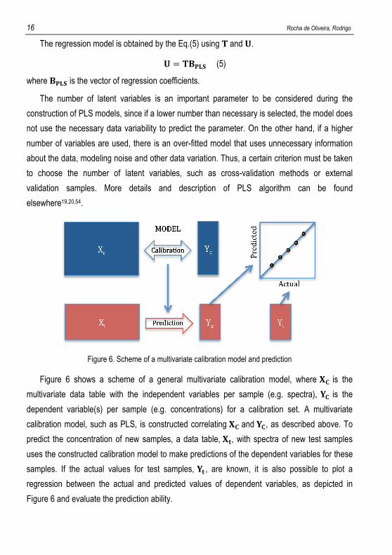
Figure 6. Scheme of a multivariate calibration model and prediction
Figure 6 shows a scheme of a general multivariate calibration model, where �* is the
multivariate data table with the independent variables per sample (e.g. spectra), �* is the
dependent variable(s) per sample (e.g. concentrations) for a calibration set. A multivariate
calibration model, such as PLS, is constructed correlating �* and �*, as described above. To
predict the concentration of new samples, a data table, �+, with spectra of new test samples
uses the constructed calibration model to make predictions of the dependent variables for these
samples. If the actual values for test samples, �+ , are known, it is also possible to plot a
regression between the actual and predicted values of dependent variables, as depicted in
Figure 6 and evaluate the prediction ability.
Design and application of chemometric methods to the determination of compounds of interest in biodiesels. 17
3.2.2. Multivariate curve resolution alternating least squares (MCR-ALS)
MCR-ALS assumes a bilinear model that is the multiwavelength extension of the Lambert-
Beer’s law25,27,55,56 and is described in matrix form by the expression,
� = *)$ + % (6)
where ��� � �� is a data matrix containing the NIR or UV-Vis spectra of the � samples for the � wavelengths recorded, *�� � ,� and )$�, � �� are the matrices with the concentration and
spectral profile of the , pure components in the samples, respectively. % has the same size of � and contains the variance not explained by the bilinear model, related to the experimental
error. In contrast to PLS, MCR-ALS does not use the matrix � to decompose the model. The
information in this matrix could be used after or during the MCR decomposition to construct
external or internal univariate calibration models with the calibration samples. Prediction of test
samples can be done during or after optimization. The procedure to make internal univariate
calibration models during the iteration is called correlation constraint and is explained in detail in
section 3.2.2.1.
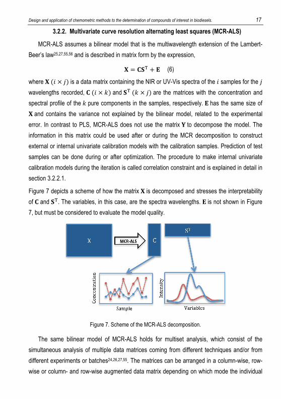
Figure 7 depicts a scheme of how the matrix � is decomposed and stresses the interpretability
of * and )$. The variables, in this case, are the spectra wavelengths. % is not shown in Figure
7, but must be considered to evaluate the model quality.
Figure 7. Scheme of the MCR-ALS decomposition.
The same bilinear model of MCR-ALS holds for multiset analysis, which consist of the
simultaneous analysis of multiple data matrices coming from different techniques and/or from
different experiments or batches24,26,27,55. The matrices can be arranged in a column-wise, row-
wise or column- and row-wise augmented data matrix depending on which mode the individual
18 Rocha de Oliveira, Rodrigo
matrices have in common57,58. A column-wise augmented matrix multiset was used in the
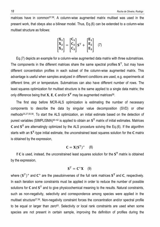
present work, that obeys also a bilinear model. Thus, Eq.(6) can be extended to a column-wise
multiset structure as follows:
-�.�/�01 = -*.*/*01 )$ +-%.%/%01 (7)
Eq.(7) depicts an example for a column-wise augmented data matrix with three submatrices.
The components in the different matrices share the same spectral profiles )$, but may have
different concentration profiles in each subset of the column-wise augmented matrix. This
advantage is useful when samples analyzed in different conditions are used, e.g. experiments at
different time, pH or temperature. Submatrices can also have different number of rows. The
least squares optimization for multiset structure is the same applied to a single data matrix; the
only difference being that �, %, * and/or ) may be augmented matrices59.
The first step before MCR-ALS optimization is estimating the number of necessary
components to describe the data by singular value decomposition (SVD) or other
methods25,27,55,56. To start the ALS optimization, an initial estimate based on the detection of
purest variables (SIMPLISMA)60–62 is applied to obtain an ) matrix of initial estimates. Matrices * and ) are alternatingly optimized by the ALS procedure solving the Eq.(6). If the algorithm
starts with an ) -type initial estimate, the unconstrained least squares solution for the * matrix
is obtained by the expression,
* = ��)$�2 (8)
If * is used, instead, the unconstrained least squares solution for the ) matrix is obtained
by the expression,
)$ = *2� (9)
where �)$�2 and *2 are the pseudoinverses of the full rank matrices ) and *, respectively.
In each iteration some constraints must be applied in order to reduce the number of possible
solutions for * and )$ and to give physicochemical meaning to the results. Natural constraints,
such as non-negativity, selectivity and correspondence among species were applied in the
multiset structure27,56. Non-negativity constraint forces the concentration and/or spectral profile
to be equal or larger than zero63. Selectivity or local rank constraints are used when some
species are not present in certain sample, improving the definition of profiles during the
Design and application of chemometric methods to the determination of compounds of interest in biodiesels. 19
iterations25. When multiset data are used, the correspondence among species constraint can be
used similarly to the selectivity constraint. In this case, a binary coded matrix sized (number of
subsets x number of components) sets the presence or absence of components in each single * subset matrix56. Another less common constraint is the correlation constraint that builds
internal univariate calibration models between reference concentration values in calibration
samples and the analogous values in MCR concentration profiles. This constraint allows
prediction of concentration values in unknown samples and provides concentration profiles in
real concentration units. This methodology has been applied successfully to quantify metal
ions64, industrial mixtures in the production process of vinyl acetate monomer65, ascorbic acid in
powder juices and tetracycline in serum samples66, steroid drugs in pharmaceutical samples,
and moisture and protein in forage samples67. This constraint was further extended for first
order data in multiset analysis and for correction of matrix effect in the determination of
paracetamol in tablets contained in blister packages using Raman spectroscopy68. Detailed
description of the correlation constraint can be found below in section 3.2.2.1.
The ALS optimization procedure finishes when a certain convergence criterion is
achieved56. Usually, the convergence is reached when the relative difference between the root
mean square of the residuals matrix % between consecutive iterations is lower than a threshold
value, commonly set to 0.1%. The quality of the MCR-ALS fit to the experimental data matrix is
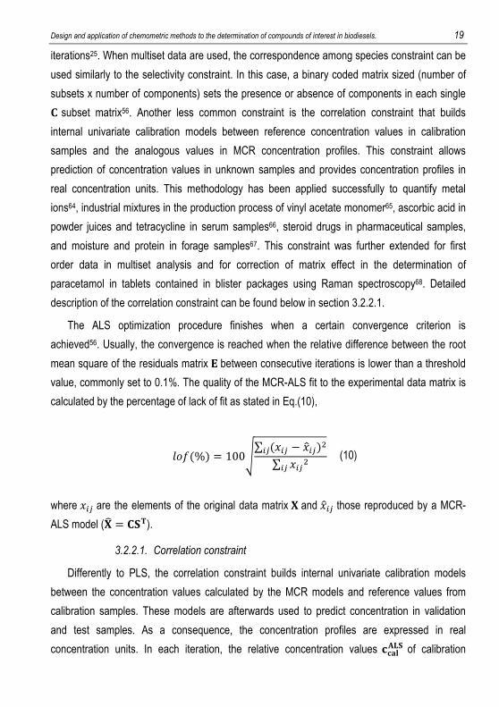
calculated by the percentage of lack of fit as stated in Eq.(10),
345�%� = 1008∑ (�� − �:�);� ∑ �� ;� (10)
where �� are the elements of the original data matrix � and �:� those reproduced by a MCR-
ALS model (�< = *) ).
3.2.2.1. Correlation constraint
Differently to PLS, the correlation constraint builds internal univariate calibration models
between the concentration values calculated by the MCR models and reference values from
calibration samples. These models are afterwards used to predict concentration in validation
and test samples. As a consequence, the concentration profiles are expressed in real
concentration units. In each iteration, the relative concentration values ==>?@() of calibration
20 Rocha de Oliveira, Rodrigo
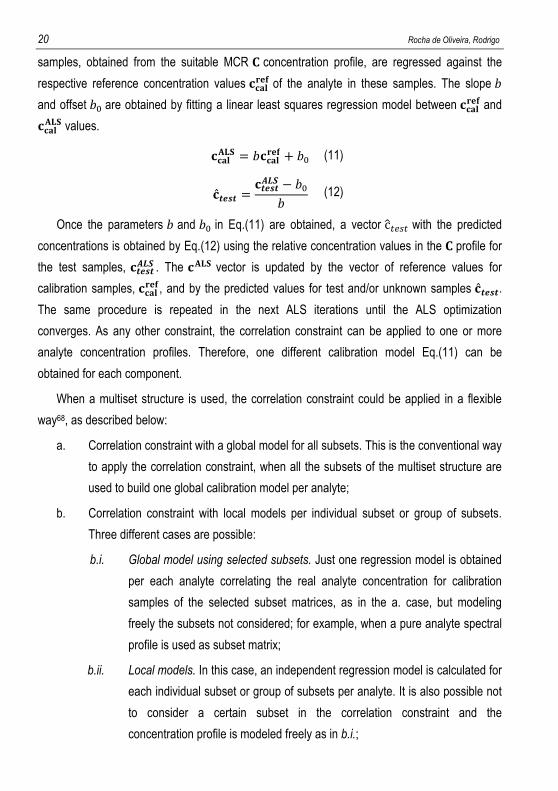
samples, obtained from the suitable MCR * concentration profile, are regressed against the
respective reference concentration values ==>?ABC of the analyte in these samples. The slope �
and offset �D are obtained by fitting a linear least squares regression model between ==>?ABC and ==>?@() values.
==>?@() = �==>?ABC + �D (11)
=FGHF = =FGHFIJK − �D� (12)
Once the parameters � and �D in Eq.(11) are obtained, a vector c:M�NM with the predicted
concentrations is obtained by Eq.(12) using the relative concentration values in the * profile for
the test samples, =FGHFIJK . The =@() vector is updated by the vector of reference values for
calibration samples, ==>?ABC, and by the predicted values for test and/or unknown samples =FGHF.
The same procedure is repeated in the next ALS iterations until the ALS optimization
converges. As any other constraint, the correlation constraint can be applied to one or more
analyte concentration profiles. Therefore, one different calibration model Eq.(11) can be
obtained for each component.
When a multiset structure is used, the correlation constraint could be applied in a flexible
way68, as described below:
a. Correlation constraint with a global model for all subsets. This is the conventional way
to apply the correlation constraint, when all the subsets of the multiset structure are
used to build one global calibration model per analyte;
b. Correlation constraint with local models per individual subset or group of subsets.
Three different cases are possible:
b.i. Global model using selected subsets. Just one regression model is obtained
per each analyte correlating the real analyte concentration for calibration
samples of the selected subset matrices, as in the a. case, but modeling
freely the subsets not considered; for example, when a pure analyte spectral
profile is used as subset matrix;
b.ii. Local models. In this case, an independent regression model is calculated for
each individual subset or group of subsets per analyte. It is also possible not
to consider a certain subset in the correlation constraint and the
concentration profile is modeled freely as in b.i.;
Design and application of chemometric methods to the determination of compounds of interest in biodiesels. 21
b.iii. Local models with matrix effect correction. The local models could also be
useful to overcome matrix effect problems between samples in different
subset matrices68. This means that there is a different relationship between
the concentration values *O and signal response �O of the analytes for each O subset affected by the matrix effect. So, the common spectral profile matrix ) is different in scale for each subset. To overcome this effect, one subset
should be taken as reference and a rescaling procedure must be applied in
the concentration values of the other subset suffering matrix effect before
updating the constrained concentration profile for the next ALS iteration. The
nonscaled vectors of real concentrations values predicted by each local
regression model for calibration and test samples are separately stored
during the analysis and recovered at the end of the MCR optimization as the
real quantitative information.
The matrix effect can be caused by different reasons such as temperature, time, sample
properties and/or variation of instrumental conditions. This effect was observed in the present
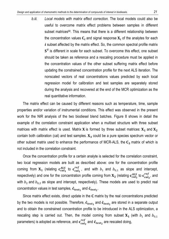
work for the NIR analysis of the two biodiesel blend batches. Figure 8 shows in detail the
example of the correlation constraint application when a multiset structure with three subset
matrices with matrix effect is used. Matrix � is formed by three subset matrices: �. and �/
contain both calibration (cal) and test samples. �0 could be a pure species spectrum vector or
other subset matrix used to enhance the performance of MCR-ALS, the *0 matrix of which is
not included in the correlation constraint.
Once the concentration profile for a certain analyte is selected for the correlation constraint,
two local regression models are built as described above: one for the concentration profile
coming from �. (relating =PQR.IJK to =PQR.SGT , and with �U and �D,U as slope and intercept,
respectively) and one for the concentration profile coming from �/ (relating =PQR/IJK to =PQR/SGT , and
with �; and �D,; as slope and intercept, respectively). These models are used to predict real
concentration values in test samples, =FGHF. and =FGHF/ .
Since matrix effect exists, direct update in the * matrix by the real concentrations predicted
by the two models is not possible. Therefore, =FGHF. and =FGHF/ are stored in a separate output
and to obtain the constrained concentration profile to be introduced in the ALS optimization, a
rescaling step is carried out. Then, the model coming from subset �. (with �U and �D,U
parameters) is adopted as reference, and =PQR/SGT and =FGHF/ are rescaled doing,
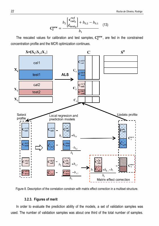
22 Rocha de Oliveira, Rodrigo
*/VBW = �; X =PQR/SGT=FGHF/Y + �D,; − �D,U�U
(13)
The rescaled values for calibration and test samples, */VBW , are fed in the constrained
concentration profile and the MCR optimization continues.
Figure 8. Description of the correlation constrain with matrix effect correction in a multiset structure.
3.2.3. Figures of merit
In order to evaluate the prediction ability of the models, a set of validation samples was
used. The number of validation samples was about one third of the total number of samples.
Design and application of chemometric methods to the determination of compounds of interest in biodiesels. 23
From the predicted Z values for these samples, some figures of merit69 were calculated
according to the following expressions.
Root mean square error of prediction (RMSEP),
RMSEP = 8∑ �Z� − Z��;�aU b (14)
Standard error of prediction (SEP),
SEP = 8∑ �Z� − Z� − ���c�;�aU b − 1 (15)
Bias,
bias = ∑ (Z� − Z�)�aU b (16)
Relative percentage error in concentration predictions (RE%),
RE�%� = 1008∑ (Z� − Z�);�aU ∑ Z�;�aU (17)
where Z� and Z� are the actual and predicted analyte concentration in sample �, respectively,
and b is the total number of samples used in the validation set.
A linear regression fit was performed between actual and predicted analyte concentration.
Slope, offset and squared correlation coefficient were also calculated. To check the similarity
between experimental and MCR-ALS recovered pure component spectral profile, a correlation
coefficient was calculated. This parameter gave a measure of how similar the shape of the
individual recovered spectral profile is to the real experimental pure component spectrum.
3.2.4. Chemometric software
Data pre-processing and PLS analysis were carried out using PLS Toolbox software
package (Eigenvector Research, Manson, WA, USA) for MATLAB (The MathWorks, Natick, MA,
USA). A graphical user interface for classical MCR-ALS by Jaumot et al.56 was used and can be
freely downloaded in the MCR web page70. Calculations of figures of merit and MCR-ALS with
the correlation constraint models were performed with laboratory-written MATLAB routines and
functions. The author participated in the implementation of the extension of the correlation

24 Rocha de Oliveira, Rodrigo
constraint to deal with high order data, such as 2D fluorescence matrices. Part of the developed
MATLAB main functions and subroutines are provided in the Appendices 1-4. A digital copy of
the complete MATLAB functions are recorded in a compact disc attached to the Appendix 5.
Design and application of chemometric methods to the determination of compounds of interest in biodiesels. 25
4. RESULTS AND DISCUSSION
4.1. ANALYSIS OF DIESEL AND BIODIESEL BLENDS
Figure 4a and Figure 4b showed the NIR spectra for the 36 diesel and biodiesel blends
before and after preprocessing, respectively, see page 14. The absorbance of the first spectral
range were multiplied by a constant scaling factor of 2.5 in order to balance the intensity
differences between the two ranges. Important bands present in the spectra are the second
overtone located in the 1150-1250 nm spectral range, the combination region at 1300-1515 nm
for the C-H stretch, the combination region for the C-H bond and combination bands for the
C=O and C-H bonds covering overlapping bands in the 2100-2500 nm spectral range33,71.
The PLS models used the matrix of preprocessed data divided in two input matrices, one
with the calibration sample spectra and the other with the test samples spectra as required by
the algorithm. Calibration samples were selected using the most influential samples in the data,
for this, the Kennard-Stones algorithm was used72. About two thirds of the total number of
samples were selected for the calibration set, and the rest were used to test the calibration
model. The leave-one-out cross validation method was used for determination of the number of
PLS latent variables (LV) by evaluating the evolution of the root mean square error of cross-
validation (RMSECV). The optimum number of latent variables was that with the lowest
RMSECV. The cross-validation model indicated two latent variables, but better results were
achieved using three, as explained below.
Model 1 in Table 2 shows the results obtained when PLS regression with two latent
variables was employed in the NIR data for prediction of biodiesel concentration. Figure 9a
shows the regression plot for the predictions of biodiesel content vs. actual values. It was
observed different linear trends in the representation of predicted versus reference values. The
samples above the � = g curve were from the second batch and the samples below, from the
first batch. This indicated that there was a batch-to-batch matrix effect. The reason could be
assigned to the long time of storage of the first batch that promoted natural ageing of the
sample mixtures. The strategy to alleviate the matrix effect was including more latent variables
in the PLS models. Model 2 shows the results when three latent variables were used. A slight
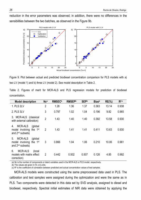
26 Rocha de Oliveira, Rodrigo
reduction in the error parameters was observed; in addition, there were no differences in the
sensibilities between the two batches, as observed in the Figure 9b.
Figure 9. Plot between actual and predicted biodiesel concentration comparison for PLS models with a)
two LV (model 1) and b) three LV (model 2). See model description in Table 2.
Table 2. Figures of merit for MCR-ALS and PLS regression models for prediction of biodiesel
concentration.
Model description Nca RMSECb RMSEPb SEPb Biasb RE(%) R2 c
1. PLS 2LV 2 1.28 1.36 1.37 0.363 13.14 0.938
2. PLS 3LV 3 0.797 1.02 1.04 0.196 9.82 0.965
3. MCR-ALS (classical with external calibration)
2 1.43 1.40 1.40 0.392 13.58 0.930
4. MCR-ALS (global model involving the 1st and 2nd subsets)
2 1.43 1.41 1.41 0.411 13.63 0.930
5. MCR-ALS (global model involving the 1st and 2nd subsets)
3 0.866 1.04 1.06 0.210 10.06 0.961
6. MCR-ALS (local models with matrix effect correction)
2 0.442 0.502 0.507 0.126 4.85 0.992
(a) Nc is the number of components or latent variables used in the MCR-ALS or PLS model, respectively. (b) The values are given in [% v/v] units. (c) R2 is the coefficient of correlation between predicted and actual concentration values of test samples.
MCR-ALS models were constructed using the same preprocessed data used in PLS. The
calibration and test samples were assigned during the optimization and were the same as in
PLS. Two components were detected in this data set by SVD analysis, assigned to diesel and
biodiesel, respectively. Spectral initial estimates of NIR data were obtained by applying the
Design and application of chemometric methods to the determination of compounds of interest in biodiesels. 27
SIMPLISMA approach62 to the multiset formed by the two batches. Before starting MCR-ALS, a
third subset matrix with the pure spectrum of neat biodiesel was input in the multiset structure,
giving a final multiset structure similar to the matrix � depicted in Figure 8, where �., �/ and �0 were the first batch, the second batch and the pure biodiesel experimental spectrum,
respectively.
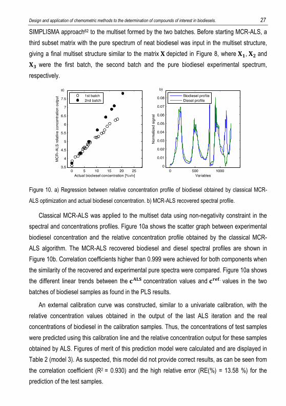
Figure 10. a) Regression between relative concentration profile of biodiesel obtained by classical MCR-
ALS optimization and actual biodiesel concentration. b) MCR-ALS recovered spectral profile.
Classical MCR-ALS was applied to the multiset data using non-negativity constraint in the
spectral and concentrations profiles. Figure 10a shows the scatter graph between experimental
biodiesel concentration and the relative concentration profile obtained by the classical MCR-
ALS algorithm. The MCR-ALS recovered biodiesel and diesel spectral profiles are shown in
Figure 10b. Correlation coefficients higher than 0.999 were achieved for both components when
the similarity of the recovered and experimental pure spectra were compared. Figure 10a shows
the different linear trends between the =@() concentration values and =ABC. values in the two
batches of biodiesel samples as found in the PLS results.
An external calibration curve was constructed, similar to a univariate calibration, with the
relative concentration values obtained in the output of the last ALS iteration and the real
concentrations of biodiesel in the calibration samples. Thus, the concentrations of test samples
were predicted using this calibration line and the relative concentration output for these samples
obtained by ALS. Figures of merit of this prediction model were calculated and are displayed in
Table 2 (model 3). As suspected, this model did not provide correct results, as can be seen from
the correlation coefficient (R2 = 0.930) and the high relative error (RE(%) = 13.58 %) for the
prediction of the test samples.
28 Rocha de Oliveira, Rodrigo
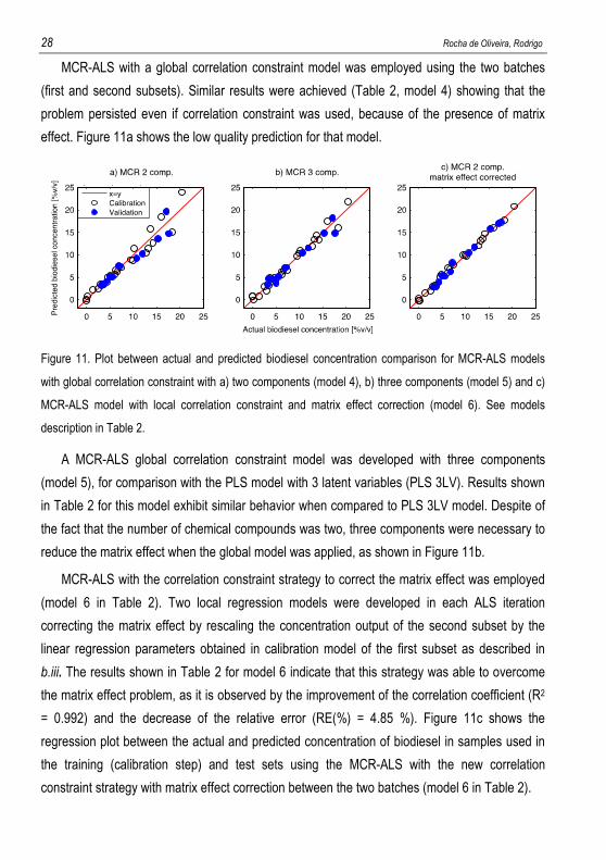
MCR-ALS with a global correlation constraint model was employed using the two batches
(first and second subsets). Similar results were achieved (Table 2, model 4) showing that the
problem persisted even if correlation constraint was used, because of the presence of matrix
effect. Figure 11a shows the low quality prediction for that model.
Figure 11. Plot between actual and predicted biodiesel concentration comparison for MCR-ALS models
with global correlation constraint with a) two components (model 4), b) three components (model 5) and c)
MCR-ALS model with local correlation constraint and matrix effect correction (model 6). See models
description in Table 2.
A MCR-ALS global correlation constraint model was developed with three components
(model 5), for comparison with the PLS model with 3 latent variables (PLS 3LV). Results shown
in Table 2 for this model exhibit similar behavior when compared to PLS 3LV model. Despite of
the fact that the number of chemical compounds was two, three components were necessary to
reduce the matrix effect when the global model was applied, as shown in Figure 11b.
MCR-ALS with the correlation constraint strategy to correct the matrix effect was employed
(model 6 in Table 2). Two local regression models were developed in each ALS iteration
correcting the matrix effect by rescaling the concentration output of the second subset by the
linear regression parameters obtained in calibration model of the first subset as described in
b.iii. The results shown in Table 2 for model 6 indicate that this strategy was able to overcome
the matrix effect problem, as it is observed by the improvement of the correlation coefficient (R2
= 0.992) and the decrease of the relative error (RE(%) = 4.85 %). Figure 11c shows the
regression plot between the actual and predicted concentration of biodiesel in samples used in
the training (calibration step) and test sets using the MCR-ALS with the new correlation
constraint strategy with matrix effect correction between the two batches (model 6 in Table 2).
Design and application of chemometric methods to the determination of compounds of interest in biodiesels. 29
None of the global combination models (PLS or MCR-ALS) with three components
outperformed the MCR-ALS model with two components and matrix effect correction. However,
including additional components in calibration models is a good alternative if a variable matrix
effect among samples exist and local models for separate sample subsets with a common
matrix effect cannot be performed67.
4.2. ANALYSIS OF BIODIESELS AND ANTIOXIDANT MIXTURES
This data was employed to show the application of correlation constraint in a more complex
situation for the determination of one kind of biodiesel and one antioxidant at low concentration
level in a mixture with biodiesels from different sources. Figure 5a and Figure 5b showed the
original and the preprocessed spectra of the 62 sample mixtures, respectively, see page 15. For
biodiesels, the main contribution for the spectral signal was from the soybean biodiesel due to
the high absorptivity of chromophores in the broad bands from 400-500 nm. The antioxidants
concentrations in the samples were very low and only PDA (N,N’-Di-sec-butyl-p-
phenylenediamine) contributed to the overall signal, but with spectral bands very overlapped
with the soybean (SB) biodiesel. The other compounds had lower signal and were completely
overlapped by the SB biodiesel compound signal. The first order SG derivative raises the
overlapped band differences between SB biodiesel and PDA in the original spectra, as
observed in Figure 5b.
PLS regression models were constructed using the preprocessed data. Calibration samples
were selected using the samples that covered the full antioxidant concentration range. About
two thirds of the total number of samples were selected for the calibration set, and the rest were
used to test the calibration model. The number of latent variables was chosen by cross-
validation. 5 latent variables were chosen for the calibration models built for the two compounds.
The results are displayed in Table 3 (models 1 and 4) for prediction of SB biodiesel and PDA,
respectively. Good prediction results were obtained for both compounds, squared correlation
coefficient between actual and predicted concentration values were superior to 0.990 and
relative error lower than 1 % and 2 %, for SB biodiesel and PDA, respectively.
MCR-ALS models were constructed and compared to PLS results. An SVD analysis was
applied to determine the number of components in the data. Four to six components could be a
reasonable choice by SVD analysis, but further analysis of the MCR-ALS and prediction results
showed that six components provided better results. MCR-ALS spectral initial estimates for the
30 Rocha de Oliveira, Rodrigo
six components were estimated by SIMPLISMA using the non-preprocessed data. That was
because the SIMPLISMA approach was not suitable for data with negative values present in the
derivative spectra. The selected initial estimates were submitted to the same preprocessing
before the MCR-ALS optimization. Due to the presence of negative values in the preprocessed
spectra, non-negativity constraint was only applied in the concentration profiles. Pure
experimental SB biodiesel and PDA antioxidant preprocessed spectrum were inserted as a
subset matrix. This strategy allows a better recovery of the spectral profiles by the MCR-ALS
models, mainly for PDA, because of the low spectral signal intensity in comparison to the
soybean (SB) biodiesel spectrum.
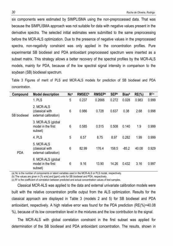
Table 3 Figures of merit of PLS and MCR-ALS models for prediction of SB biodiesel and PDA
concentration.
Compound Model description Nca RMSECb RMSEPb SEPb Biasb RE(%) R2 c
SB biodiesel
1. PLS 5 0.237 0.2666 0.272 0.028 0.983 0.999
2. MCR-ALS (classical with external calibration)
6 0.986 0.728 0.637 0.38 2.68 0.998
3. MCR-ALS (global model in the first subset)
6 0.585 0.515 0.508 0.140 1.9 0.999
PDA
4. PLS 5 6.57 8.75 8.97 0.282 1.99 0.999
5. MCR-ALS (classical with external calibration)
6 82.99 176.4 158.5 -85.2 40.08 0.929
6. MCR-ALS (global model in the first subset)
6 9.16 13.90 14.26 0.432 3.16 0.997
(a) Nc is the number of components or latent variables used in the MCR-ALS or PLS model, respectively. (b) The values are given in [% w/w] and [ppm] units for SB biodiesel and PDA, respectively. (c) R2 is the coefficient of correlation between predicted and actual concentration values of test samples.
Classical MCR-ALS was applied to the data and external univariate calibration models were
built with the relative concentration profile output from the ALS optimization. Results for the
classical approach are displayed in Table 3 (models 2 and 5) for SB biodiesel and PDA
antioxidant, respectively. A high relative error was found for the PDA prediction (RE(%)=40.08
%), because of its low concentration level in the mixtures and the low contribution to the signal.
The MCR-ALS with global correlation constraint in the first subset was applied for
determination of the SB biodiesel and PDA antioxidant concentration. The results, shown in
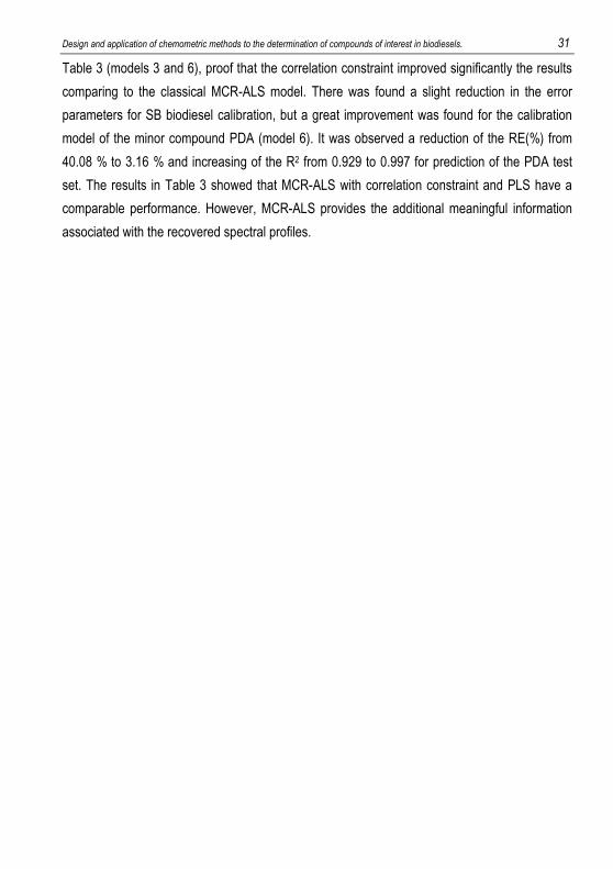
Design and application of chemometric methods to the determination of compounds of interest in biodiesels. 31
Table 3 (models 3 and 6), proof that the correlation constraint improved significantly the results
comparing to the classical MCR-ALS model. There was found a slight reduction in the error
parameters for SB biodiesel calibration, but a great improvement was found for the calibration
model of the minor compound PDA (model 6). It was observed a reduction of the RE(%) from
40.08 % to 3.16 % and increasing of the R2 from 0.929 to 0.997 for prediction of the PDA test
set. The results in Table 3 showed that MCR-ALS with correlation constraint and PLS have a
comparable performance. However, MCR-ALS provides the additional meaningful information
associated with the recovered spectral profiles.

Design and application of chemometric methods to the determination of compounds of interest in biodiesels. 33
CONCLUSIONS The MCR-ALS method with the correlation constraint in the multiset approach has been
demonstrated to be a useful and accurate tool for quantification of biodiesel blend level using
NIR spectroscopy and biodiesel and synthetic PDA antioxidant in biodiesel mixtures using UV-
Visible spectroscopy. The recent modification in the correlation constraint to correct the batch-
to-batch matrix effect found between ageing biodiesel/diesel blends was successfully applied in
this work. Only slightly worse results were obtained by increasing the number of components in
the MCR-ALS modeling, as was proven to happen in PLS regression models to alleviate the
matrix effect. It is useful in cases where there is a variable and insufficient defined matrix effect.
The correlation constraint was also applied for a complex case where a minor antioxidant
compound with an overlapped signal with other compounds had to be determined. It was shown
that the correlation constraint was crucial to improve the recovered profiles and prediction
results in comparison to classical MCR-ALS models with a posteriori building of calibration
models.

Design and application of chemometric methods to the determination of compounds of interest in biodiesels. 35
REFERENCES 1. Singh, S. P.; Singh, D. Biodiesel production through the use of different sources and characterization
of oils and their esters as the substitute of diesel: A review. Renewable Sustainable Energy Rev. 2010, 14, 200–216.
2. Knothe, G.; Dunn, R. O.; Bagby, M. O. Biodiesel: The Use of Vegetable Oils and Their Derivatives as Alternative Diesel Fuels. ACS Symp. Ser. 1997, 666, 172–208.
3. Salvi, B. L.; Subramanian, K. A.; Panwar, N. L. Alternative fuels for transportation vehicles: A technical review. Renewable Sustainable Energy Rev. 2013, 25, 404–419.
4. Monteiro, M. R.; Ambrozin, A. R. P.; Lião, L. M.; Ferreira, A. G. Critical review on analytical methods for biodiesel characterization. Talanta 2008, 77, 593–605.
5. Knothe, G. Some aspects of biodiesel oxidative stability. Fuel Process. Technol. 2007, 88, 669–677. 6. Felizardo, P.; Neiva Correia, M. J.; Raposo, I.; Mendes, J. F.; Berkemeier, R.; Bordado, J. M.; Correia,
M. J. N. Production of biodiesel from waste frying oils. Waste Manage. 2006, 26, 487–494. 7. Biodiesel Handling and Use Guide, Fourth Edition. National Renewable Energy Laboratory, U.S.
Department of Energy.; Oak Ridge, TN, 2009. 8. Leung, D. Y. C.; Wu, X.; Leung, M. K. H. A review on biodiesel production using catalyzed
transesterification. Appl. Energy 2010, 87, 1083–1095. 9. Enweremadu, C. C.; Mbarawa, M. M. Technical aspects of production and analysis of biodiesel from
used cooking oil—A review. Renewable Sustainable Energy Rev. 2009, 13, 2205–2224. 10. Gog, A.; Roman, M.; Toşa, M.; Paizs, C.; Irimie, F. D. Biodiesel production using enzymatic
transesterification – Current state and perspectives. Renewable Energy 2012, 39, 10–16. 11. Jain, S.; Sharma, M. P. Stability of biodiesel and its blends: A review. Renewable Sustainable Energy
Rev. 2010, 14, 667–678. 12. Dunn, R. O. Effect of antioxidants on the oxidative stability of methyl soyate ( biodiesel ) B. Fuel
Process. Technol. 2005, 86, 1071–1085. 13. Aquino, I. P.; Hernandez, R. P. B.; Chicoma, D. L.; Pinto, H. P. F.; Aoki, I. V. Influence of light,
temperature and metallic ions on biodiesel degradation and corrosiveness to copper and brass. Fuel 2012, 102, 795–807.
14. Focke, W. W.; Westhuizen, I. Van Der; Grobler, A. B. L.; Nshoane, K. T.; Reddy, J. K.; Luyt, A. S. The effect of synthetic antioxidants on the oxidative stability of biodiesel. Fuel 2012, 94, 227–233.
15. Lapuerta, M.; Rodríguez-Fernández, J.; Ramos, Á.; Álvarez, B. Effect of the test temperature and anti-oxidant addition on the oxidation stability of commercial biodiesel fuels. Fuel 2012, 93, 391–396.
16. Dinkov, R.; Hristov, G.; Stratiev, D.; Aldayri, V. B. Effect of commercially available antioxidants over biodiesel/diesel blends stability. Fuel 2009, 88, 732–737.
17. IUPAC Compendium of Chemical Terminology; Nič, M.; Jirát, J.; Košata, B.; Jenkins, A.; McNaught, A., Eds.; 2nd ed.; IUPAC: Research Triagle Park, NC, 2009.
18. Massart, D. L.; Vandeginste, B.G.M. Buydens, L. M. C.; de Jong, S.; Lewi, P. J.; Smeyers-Verbeke, J. Handbook of Chemometrics and Qualimetrics. Part A. In Data Handling in Science and Technology 20A; Elsevier Science B.V.: Amsterdam, 1997.
19. Martens, H.; Naes, T. Multivariate Calibration; Wiley: New York, 1991. 20. Thomas, E. V. A Primer on Multivariate Calibration. Anal. Chem. 1994, 66, 795A–804A. 21. de Juan, A.; Tauler, R. Chemometrics applied to unravel multicomponent processes and mixtures.
Anal. Chim. Acta 2003, 500, 195–210.
36 Rocha de Oliveira, Rodrigo
22. de Juan, A.; Tauler, R. Multivariate Curve Resolution (MCR) from 2000: Progress in Concepts and Applications. Crit. Rev. Anal. Chem. 2006, 36, 163–176.
23. Gargallo, R.; Tauler, R.; Cuesta-Sánchez, F.; Massart, D. L. Validation of alternating least-squares multivariate curve resolution for chromatographic resolution and quantitation. TrAC, Trends Anal. Chem. 1996, 15, 279–286.
24. Tauler, R.; Barceló, D. Multivariate curve resolution applied to liquid chromatography-diode array detection. TrAC, Trends Anal. Chem. 1993, 12, 319–327.
25. Tauler, R.; Smilde, A.; Kowalski, B. R. Selectivity , local rank , three-way data analysis and ambiguity in multivariate curve resolution. J. Chemom. 1995, 9, 31–58.
26. Tauler, R.; Smilde, A. K.; Henshaw, J. M.; Burgess, L. W.; Kowalski, B. R. Multicomponent Determination of Chlorinated Hydrocarbons Using a Reaction-Based Chemical Sensor . 2 . Chemical Speciation Using Multivariate Curve Resolution. Anal. Chem. 1994, 66, 3337–3344.
27. Tauler, R.; Kowalski, B. R.; Fleming, S. Multivariate Curve Resolution Applied to Spectral Data from Multiple Runs of an Industrial Process. Anal. Chem. 1993, 65, 2040–2047.
28. Souza, F. H. N.; de Almeida, L. R.; Batista, F. S. C. L.; Rios, M. A. de S. UV-Visible Spectroscopy Study of Oxidative Degradation of Sunflower Biodiesel. Energy Sci. Technol. 2011, 2, 56–61.
29. de Vasconcelos, F. V. C.; de Souza, P. F. B.; Pimentel, M. F.; Pontes, M. J. C.; Pereira, C. F. Using near-infrared overtone regions to determine biodiesel content and adulteration of diesel/biodiesel blends with vegetable oils. Anal. Chim. Acta 2012, 716, 101–7.
30. Zawadzki, A.; Shrestha, D. S.; He, B. Biodiesel blend level detection using ultraviolet absorption spectra. Trans. ASABE 2007, 50, 1349–1353.
31. Rocha, W. F.; Nogueira, R.; Vaz, B. G. Validation of model of multivariate calibration: an application to the determination of biodiesel blend levels in diesel by near-infrared spectroscopy. J. Chemom. 2012, 26, 456–461.
32. Fernandes, D. D. S.; Gomes, A. A.; da Costa, G. B.; da Silva, G. W. B.; Véras, G. Determination of biodiesel content in biodiesel/diesel blends using NIR and visible spectroscopy with variable selection. Talanta 2011, 87, 30–4.
33. Zhang, W. Review on analysis of biodiesel with infrared spectroscopy. Renewable Sustainable Energy Rev. 2012, 16, 6048–6058.
34. Alves, J. C. L.; Poppi, R. J. Biodiesel content determination in diesel fuel blends using near infrared (NIR) spectroscopy and support vector machines (SVM). Talanta 2013, 104, 155–61.
35. Balabin, R. M.; Lomakina, E. I.; Safieva, R. Z. Neural network (ANN) approach to biodiesel analysis: Analysis of biodiesel density, kinematic viscosity, methanol and water contents using near infrared (NIR) spectroscopy. Fuel 2011, 90, 2007–2015.
36. Gaydou, V.; Kister, J.; Dupuy, N. Evaluation of multiblock NIR/MIR PLS predictive models to detect adulteration of diesel/biodiesel blends by vegetal oil. Chemom. Intell. Lab. Syst. 2011, 106, 190–197.
37. Veras, G.; Gomes, A. D. A.; da Silva, A. C.; de Brito, A. L. B.; de Almeida, P. B. A.; de Medeiros, E. P. Classification of biodiesel using NIR spectrometry and multivariate techniques. Talanta 2010, 83, 565–8.
38. Caires, A. R. L.; Lima, V. S.; Oliveira, S. L. Quantification of biodiesel content in diesel/biodiesel blends by fluorescence spectroscopy: Evaluation of the dependence on biodiesel feedstock. Renewable Energy 2012, 46, 137–140.
39. Insausti, M.; Gomes, A. A.; Cruz, F. V; Pistonesi, M. F.; Araujo, M. C. U.; Galvão, R. K. H.; Pereira, C. F.; Band, B. S. F. Screening analysis of biodiesel feedstock using UV-vis, NIR and synchronous fluorescence spectrometries and the successive projections algorithm. Talanta 2012, 97, 579–83.
40. Balabin, R. M.; Smirnov, S. V. Variable selection in near-infrared spectroscopy: benchmarking of feature selection methods on biodiesel data. Anal. Chim. Acta 2011, 692, 63–72.
41. Tormin, T. F.; Gimenes, D. T.; Silva, L. G.; Ruggiero, R.; Richter, E. M.; Ferreira, V. S.; Muñoz, R. A. A. Direct amperometric determination of tert-butylhydroquinone in biodiesel. Talanta 2010, 82, 1599–603.
Design and application of chemometric methods to the determination of compounds of interest in biodiesels. 37
42. Tormin, T. F.; Gimenes, D. T.; Richter, E. M.; Muñoz, R. A. A. Fast and direct determination of butylated hydroxyanisole in biodiesel by batch injection analysis with amperometric detection. Talanta 2011, 85, 1274–1278.
43. Tormin, T. F.; Cunha, R. R.; Richter, E. M.; Muñoz, R. A. A. Fast simultaneous determination of BHA and TBHQ antioxidants in biodiesel by batch injection analysis using pulsed-amperometric detection. Talanta 2012, 99, 527–31.
44. Alberici, R. M.; Simas, R. C.; Abdelnur, P. V; Eberlin, M. N.; Souza, V. de; Sá, G. F. de A Highly Effective Antioxidant and Artificial Marker for Biodiesel. Energy Fuels 2010, 24, 6522–6526.
45. Batista, L. N.; Silva, V. F.; Fonseca, M. G.; Pissurno, E. C. G.; Daroda, R. J.; Cunha, V. S.; Kunigami, C. N.; de Santa Maria, L. C. Easy to use spectrophotometric method for determination of aromatic diamines in biodiesel samples. Microchem. J. 2013, 106, 17–22.
46. del Río, V.; Larrechi, M. S.; Callao, M. P. Determination of sulphate in water and biodiesel samples by a sequential injection analysis--multivariate curve resolution method. Anal. Chim. Acta 2010, 676, 28–33.
47. del Río, V.; Larrechi, M. S.; Callao, M. P. Sequential injection titration method using second-order signals: determination of acidity in plant oils and biodiesel samples. Talanta 2010, 81, 1572–7.
48. Baynox Solution. http://www.biofuelsystems.com/other/baynox_solution_data.pdf (accessed Jan 12, 2013).
49. SANTOFLEX 44PD. http://www.solutia.com/pdf/MSDS/SANTOFLEX 44PD-LIQ 921101_GB_GB UK.pdf (accessed Jan 12, 2013).
50. Kramer, K. E.; Morris, R. E.; Rose-Pehrsson, S. L. Comparison of two multiplicative signal correction strategies for calibration transfer without standards. Chemom. Intell. Lab. Syst. 2008, 92, 33–43.
51. Savitzky, A.; Golay, M. J. E. Smoothing and Differentiation of Data by Simplified Least Squares Procedures. Anal. Chem. 1964, 36, 1627–1639.
52. Brereton, R. G. Introduction to multivariate calibration in analytical chemistry. Analyst 2000, 125, 2125–2154.
53. Booksh, K. S.; Kowalski, B. R. Theory of Analytical Chemistry. Anal. Chem. 1994, 66, 782A–791A. 54. Haaland, D. M.; Thomas, E. V. Partial Least-Squares Methods for Spectral Analyses . 1 . Relation to
Other Quantitative Calibration Methods and the Extraction of Qualitative Information. Anal. Chem. 1988, 60, 1193–1202.
55. Tauler, R. Multivariate curve resolution applied to second order data. Chemom. Intell. Lab. Syst. 1995, 30, 133–146.
56. Jaumot, J.; Gargallo, R.; de Juan, A.; Tauler, R. A graphical user-friendly interface for MCR-ALS: a new tool for multivariate curve resolution in MATLAB. Chemom. Intell. Lab. Syst. 2005, 76, 101–110.
57. Alier, M.; Felipe, M.; Hernàndez, I.; Tauler, R. Variation patterns of nitric oxide in Catalonia during the period from 2001 to 2006 using multivariate data analysis methods. Anal. Chim. Acta 2009, 642, 77–88.
58. Alier, M.; Felipe, M.; Hernández, I.; Tauler, R. Trilinearity and component interaction constraints in the multivariate curve resolution investigation of NO and O3 pollution in Barcelona. Anal. Bioanal. Chem. 2011, 399, 2015–29.
59. Tauler, R.; Maeder, M.; de Juan, A. Multiset Data Analysis: Extended Multivariate Curve Resolution. In Comprehensive chemometrics: chemical and biochemical data analysis four-volume set. Vol. 2, Chapter 2.24, S.D. Brown, R. Tauler, B. Walczak; Elsevier, 2009; Vol. 2, pp. 473–505.
60. Windig, W.; Guilment, J. Interactive Self-Modeling Mixture Analysis. Anal. Chem. 1991, 63, 1425–1432.
61. Windig, W.; Stephenson, D. A. Self-Modeling Mixture Analysis of Second-Derivative Near-Infrared Spectral Data Using the Simplisma Approach. Anal. Chem. 1992, 64, 2735–2742.
62. Windig, W. Spectral data files for self-modeling curve resolution with examples using the Simplisma approach. Chemom. Intell. Lab. Syst. 1997, 36, 3–16.
63. Bro, R.; Jong, S. A fast non-negativity-constrained least squares algorithm. J. Chemom. 1997, 11, 393–401.
38 Rocha de Oliveira, Rodrigo
64. Antunes, M. C.; Simão, J. E. J.; Duarte, A. C.; Tauler, R. Multivariate curve resolution of overlapping voltammetric peaks: quantitative analysis of binary and quaternary metal mixtures. Analyst 2002, 127, 809–817.
65. Richards, S. E.; Becker, E.; Tauler, R.; Walmsley, A. D. A novel approach to the quantification of industrial mixtures from the Vinyl Acetate Monomer (VAM) process using Near Infrared spectroscopic data and a Quantitative Self Modeling Curve Resolution (SMCR) methodology. Chemom. Intell. Lab. Syst. 2008, 94, 9–18.
66. Goicoechea, H. C.; Olivieri, A. C.; Tauler, R. Application of the correlation constrained multivariate curve resolution alternating least-squares method for analyte quantitation in the presence of unexpected interferences using first-order instrumental data. Analyst 2010, 135, 636–642.
67. Azzouz, T.; Tauler, R. Application of multivariate curve resolution alternating least squares (MCR-ALS) to the quantitative analysis of pharmaceutical and agricultural samples. Talanta 2008, 74, 1201–1210.
68. Lyndgaard, L. B.; Van den Berg, F.; de Juan, A. Quantification of paracetamol through tablet blister packages by Raman spectroscopy and multivariate curve resolution-alternating least squares. Chemom. Intell. Lab. Syst. 2013, 125, 58–66.
69. Olivieri, A. C.; Faber, N. M.; Ferré, J.; Boqué, R.; Kalivas, J. H.; Mark, H. Uncertainty estimation and figures of merit for multivariate calibration (IUPAC Technical Report). Pure. Appl. Chem. 2006, 78, 633–661.
70. MCR web page. http://www.mcrals.info (accessed Jan 12, 2013). 71. Xiaobo, Z.; Jiewen, Z.; Povey, M. J. W.; Holmes, M.; Hanpin, M. Variables selection methods in near-
infrared spectroscopy. Anal. Chim. Acta 2010, 667, 14–32. 72. Kennard, R. W.; Stone, L. A. Computer Aided Design of Experiments. Technometrics 1969, 11, 137–
148.

Design and application of chemometric methods to the determination of compounds of interest in biodiesels. 39
APPENDICES

40 Rocha de Oliveira, Rodrigo
Design and application of chemometric methods to the determination of compounds of interest in biodiesels. 41
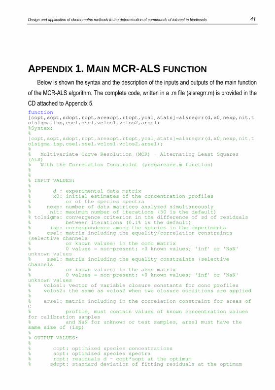
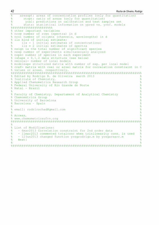
APPENDIX 1. MAIN MCR-ALS FUNCTION Below is shown the syntax and the description of the inputs and outputs of the main function
of the MCR-ALS algorithm. The complete code, written in a .m file (alsregrr.m) is provided in the
CD attached to Appendix 5. function [copt,sopt,sdopt,ropt,areaopt,rtopt,ycal,stats]=als regrr(d,x0,nexp,nit,tolsigma,isp,csel,ssel,vclos1,vclos2,arsel) %Syntax: % [copt,sopt,sdopt,ropt,areaopt,rtopt,ycal,stats]=als regrr(d,x0,nexp,nit,tolsigma,isp,csel,ssel,vclos1,vclos2,arsel); % % Multivariate Curve Resolution (MCR) - Alternati ng Least Squares (ALS) % With the Correlation Constraint (yregarearr.m f unction) % % % INPUT VALUES: % % d : experimental data matrix % x0: initial estimates of the concentration profiles % or of the species spectra % nexp: number of data matrices analyzed simult aneously % nit: maximum number of iterations (50 is the default) % tolsigma: convergence criterion in the difference of sd of residuals % between iterations (0.1% is the default ) % isp: correspondence among the species in the experiments % csel: matrix including the equality/correlati on constraints (selective channels % or known values) in the conc matrix % 0 values = non-present; >0 known values ; 'inf' or 'NaN' unknown values % ssel: matrix including the equality constrain ts (selective channels % or known values) in the abss matrix % 0 values = non-present; >0 known values ; 'inf' or 'NaN' unknown values % vclos1: vector of variable closure constants f or conc profiles % vclos2: the same as vclos2 when two closure co nditions are applied % % arsel: matrix including in the correlation con straint for areas of C % profile, must contain values of known c oncentration values for calibration samples % and NaN for unknown or test samples, ar sel must have the same size of (isp) % % OUTPUT VALUES: % % copt: optimized species concentrations % sopt: optimized species spectra % ropt: residuals d - copt*sopt at the optimu m % sdopt: standard deviation of fitting residua ls at the optimum
42 Rocha de Oliveira, Rodrigo
% areaopt: areas of concentration profiles (only for quantitation) % rtopt: ratio of areas (only for quantitation ) % ycal: predictions on calibration and test s amples set % stats: statistical information on ypred vs. yref. models %%%%%%%%%%%%%%%%%%%%%%% % other important variables % nrow number of rows (spectra) in d % ncol number of columns (channels, wavelengths) in d % ils kind of initial estimate; % ils = 1 initial estimates of concentrations; % ils = 2 initial estimates of spectra % nsign is the total number of significant species % nexp number of experiments simultaneously analyze d % nspec number of species in each experiment % ishape = 0,1,2 data structure (see below) % nmlocal= number of local models % modelexp= structured matrix with number of exp. p er local model % cref= matrix with csel or arsel matrix for correl ation constraint in C % values or areas, respectively. %%%%%%%%%%%%%%%%%%%%%%%%%%%%%%%%%%%%%%%%%%%%%%%%%%%%%%%%%%%%%%%%%%%%%%%% % Edited by Rodrigo R. de Oliveira march 2013 % % Institute of Chemistry, % % Applied Chemometrics Research Group % % Federal University of Rio Grande do Norte % % Natal - Brazil % % % % Faculty of Chemistry, Departament of Analytical C hemistry % % Chemometrics Group % % University of Barcelona % % Barcelona - Spain % % % % email: [email protected] % % % % Access, % % www.chemometricsufrn.org % %%%%%%%%%%%%%%%%%%%%%%%%%%%%%%%%%%%%%%%%%%%%%%%%%%%%%%%%%%%%%%%%%%%%%%%% % % % List of Modifications: % % - 6mar2013 Correlation constraint for 2nd order data % % - 11mar2013 commented totalconc when trinlinear ity cons. is used % % - 12jun2013 changed function yregrodrigo.m by y regarearr.m % % Next: % % % %%%%%%%%%%%%%%%%%%%%%%%%%%%%%%%%%%%%%%%%%%%%%%%%%%%%%%%%%%%%%%%%%%%%%%%%
Design and application of chemometric methods to the determination of compounds of interest in biodiesels. 43
APPENDIX 2. SUBROUTINE 1 The code below represents the subroutine written inside the main function (alsregrr.m) to
interact with the user and initializes the correlation constraint subroutines.
%% ******************************************** ****** % EQUALITY/CORRELATION CONSTRAINTS IN CONC PROFILES * %************************************************** ** cons4 = find(wcons == 4); % in input matrix csel finite values are known if ~isempty(cons4) iisel=find(isfinite(csel)); if isempty(csel) && isempty(arsel) disp( ' ' );disp( ' ' );disp( ' ' ) disp( 'conc and area equality/correlation constraint matr ices csel and arsel were not input' ) return else disp( ' ' );disp( ' ' );disp( ' ' ) disp( 'CONC EQUALITY/CORRELATION CONSTRAINTS WILL BE APPL IED !!!!' ), disp( 'Apply correlation constraint?' ) disp( '(0) No;' ) disp( '(1) in values of C profile;' ) if nexp>1 disp( '(2) in areas of C profile;' ) iregr=input( 'Option (0, 1, 2): ' ); else iregr=input( 'Option (0, 1): ' ); end %%% Check for correlation/equality constraints inpu ts if (iregr==1||iregr==0) && isempty(csel) disp( ' ' );disp( ' ' );disp( ' ' ) disp( 'conc equality/correlation constraints matrix csel was not input' ) return end if iregr==1 || iregr==2 compreg=input( 'Compounds to perform regression? e.g. only 1st, [1 0 0] ' ); if matc>1 disp( ' ' ) regmodel=input( 'Global regression model (0) or local regression per C submatrices (1)? ' ); if regmodel==0 nmlocal=1; modelexp{1,1}=input([ 'Which experiments to include in the global model? (if all, enter: [1:' ,num2str(nexp), '])' ]); % select some experiments for global models elseif regmodel==1 disp( 'Local regression per C submatrices!' ) nmlocal=input( 'How many local models? ' ); modelexp=cell(nmlocal,1); disp( ' ' ) for mi=1:nmlocal

44 Rocha de Oliveira, Rodrigo
disp([ 'Model ' ,num2str(mi)]); modelexp{mi,1}=input( 'Which submatrices? ' ); end if nmlocal>1 mateffect=input( 'Is there matrix effect among models,i.e., different slopes? YES(1), NO(0)' ); end end end else disp( ' ' );disp( ' ' );disp( ' ' ) disp( 'ONLY CONC. EQUALITY CONSTRAINTS WILL BE APPLIED !!!!' ) end end end
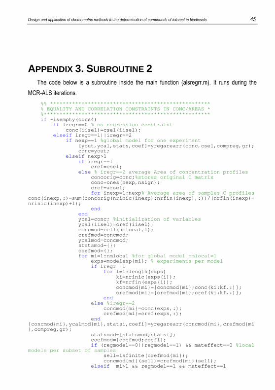
Design and application of chemometric methods to the determination of compounds of interest in biodiesels. 45
APPENDIX 3. SUBROUTINE 2 The code below is a subroutine inside the main function (alsregrr.m). It runs during the
MCR-ALS iterations.
%% ******************************************** ******* % EQUALITY AND CORRELATION CONSTRAINTS IN CONC/AREAS * %************************************************** *** if ~isempty(cons4) if iregr==0 % no regression constraint conc(iisel)=csel(iisel); elseif iregr==1||iregr==2 if nexp==1 %global model for one experiment [yout,ycal,stats,coef]=yregarearr(c onc,csel,compreg,gr); conc=yout; elseif nexp>1 if iregr==1 cref=csel; else % iregr==2 average Area of concentration profiles concorig=conc; %stores original C matrix conc=ones(nexp,nsign); cref=arsel; for inexp=1:nexp % Average area of samples C profiles conc(inexp,:)=sum(concorig(nrinic(inexp):nrfin(inex p),:))/(nrfin(inexp)-nrinic(inexp)+1); end end ycal=conc; %initialization of variables ycal(iisel)=cref(iisel); concmod=cell(nmlocal,1); crefmod=concmod; ycalmod=concmod; statsmod={}; coefmod={}; for mi=1:nmlocal %for global model nmlocal=1 exps=modelexp{mi}; % experiments per model if iregr==1 for i=1:length(exps) ki=nrinic(exps(i)); kf=nrfin(exps(i)); concmod{mi}=[concmod{mi };conc(ki:kf,:)]; crefmod{mi}=[crefmod{mi };cref(ki:kf,:)]; end else %iregr==2 concmod{mi}=conc(exps,:); crefmod{mi}=cref(exps,:); end [concmod{mi},ycalmod{mi},statsi,coefi]=yregarearr(c oncmod{mi},crefmod{mi},compreg,gr); statsmod=[statsmod;statsi]; coefmod=[coefmod;coefi]; if (regmodel==0||regmodel==1) && mateffect==0 %local models per subset of samples sell=isfinite(crefmod{mi}); concmod{mi}(sell)=crefmod{m i}(sell); elseif mi>1 && regmodel==1 && mateffect==1
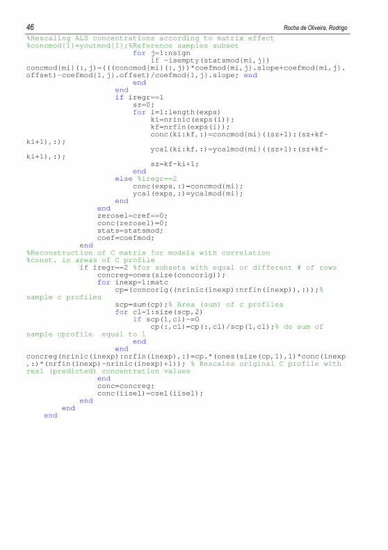
46 Rocha de Oliveira, Rodrigo
%Rescaling ALS concentrations according to matrix e ffect %concmod{1}=youtmod{1};%Reference samples subset for j=1:nsign if ~isempty(statsmod{mi,j}) concmod{mi}(:,j)=(((concmod{mi}(:,j))*coefmod{mi,j} .slope+coefmod{mi,j}.offset)-coefmod{1,j}.offset)/coefmod{1,j}.slope; end end end if iregr==1 sz=0; for i=1:length(exps) ki=nrinic(exps(i)); kf=nrfin(exps(i)); conc(ki:kf,:)=concmod{m i}((sz+1):(sz+kf-ki+1),:); ycal(ki:kf,:)=ycalmod{m i}((sz+1):(sz+kf-ki+1),:); sz=kf-ki+1; end else %iregr==2 conc(exps,:)=concmod{mi}; ycal(exps,:)=ycalmod{mi}; end end zerosel=cref==0; conc(zerosel)=0; stats=statsmod; coef=coefmod; end %Reconstruction of C matrix for models with correla tion %const. in areas of C profile if iregr==2 %for subsets with equal or different # of rows concreg=ones(size(concorig)); for inexp=1:matc cp=(concorig((nrinic(inexp):nrf in(inexp)),:)); % sample c profiles scp=sum(cp); % Area (sum) of c profiles for cl=1:size(scp,2) if scp(1,cl)~=0 cp(:,cl)=cp(:,cl)/scp(1 ,cl); % do sum of sample cprofile equal to 1 end end concreg(nrinic(inexp):nrfin(inexp),:)=cp.*(ones(siz e(cp,1),1)*conc(inexp,:)*(nrfin(inexp)-nrinic(inexp)+1)); % Rescales original C profile with real (predicted) concentration values end conc=concreg; conc(iisel)=csel(iisel); end end end
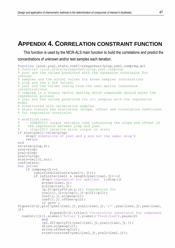
Design and application of chemometric methods to the determination of compounds of interest in biodiesels. 47
APPENDIX 4. CORRELATION CONSTRAINT FUNCTION This function is used by the MCR-ALS main function to build the correlations and predict the
concentrations of unknown and/or test samples each iteration.
function [yout,ycal,stats,coef]=yregarearr(yinp,ysel,compre g,gr) % function [yout,stats]=yregarearr(yinp,ysel,compre g) % yout are the values predicted with the rgression constraint for unknown % samples and the actual values for known samples ( calibration) % yinp are the y ALS values; % ysel are the values coming from the csel matrix ( reference concentrations) % compreg is a binary vector setting which compound s should enter the regression process % ycal are the values predicted for all samples wit h the regression model % constructed with calibration samples % stats contain tha statistics (slope, offset and c orrelation coeficient % for regression constraint % modifications: % - 22MAR2013 output variable coef containing the slope and offset of % the regression between yimp and ysel % - 11apr2013 relative error output in stats if size(ysel)~=size(yinp) disp( 'dimensions of ysel and y are not the same; stop' ) return end nc=size(yinp,2); yout=yinp; ycal=yinp; ycalc=yinp; stats=cell(1,nc); coef=stats; for j=1:nc if compreg(j)==1 isel=find(isfinite(ysel(:,j))); if isfinite(isel) & length(ysel(isel,j))>=2 disp( 'regression for species: ' );disp(j) x=ysel(isel,j); y=yinp(isel,j); [p,S]=polyfit(x,y,1); %regression fit ycalc(:,j)=(yinp(:,j)-p(2))/p(1); coef{1,j}.slope=p(1); coef{1,j}.offset=p(2); if gr== 'y' figure(2+j),plot(ysel(isel,j),ycalc(isel,j), 'r*' ,ysel(isel,j),ysel(isel,j)) figure(2+j),title([ 'Correlation constraint for component ' num2str(j)]),xlabel( 'Actual' ),ylabel( 'Predicted' ),pause(2) end [p2,S2]=polyfit(ysel(isel,j),ycalc(isel ,j),1); stind.slope=p2(1); stind.offset=p2(2); rcoef=corrcoef(ysel(isel,j),ycalc(isel, j));

48 Rocha de Oliveira, Rodrigo
stind.r=rcoef(1,2); stind.RMSEC=S2.normr/sqrt(length(x)); dev=ysel(isel,j)-ycalc(isel,j); erel=100*sqrt(dev'*dev/(ysel(isel,j)'*y sel(isel,j))); % relative error also useful to know stind.erel=erel; ycal(:,j)=ycalc(:,j); ycalc(isel,j)=ysel(isel,j); yout(:,j)=ycalc(:,j); stats{1,j}=stind; end end end end

Design and application of chemometric methods to the determination of compounds of interest in biodiesels. 49
APPENDIX 5. COMPACT DISC This CD contains the functions developed during the work to perform the MCR-ALS models.
This version includes extension of the correlation constraint developed to correlate the profiles
areas obtained by MCR with the concentrations in cases where high order data are employed,
such as excitation x emission fluorescence matrices.
CD