Embed Size (px)
Citation preview
Treball Final de Grau
Tutor/s
Dr. Jordi Bonet Ruiz Department of Chemical Engineering
Dr. Joan Llorens Llacuna Department of Chemical Engineering
Fluid circulation simulation in heat exchangers:
Shell and tube (CFD - ANSYS®)
Simulació de la circulació de fluids en bescanviadors de calor:
Carcassa i tubs (CFD - ANSYS®)
Gerard Minella Sivill June 2016


Aquesta obra està subjecta a la llicència de: Reconeixement–NoComercial-SenseObraDerivada
http://creativecommons.org/licenses/by-nc-nd/3.0/es/


Si no conozco alguna cosa, la investigaré
Louis Pasteur
En primer lloc voldria donar les gràcies als meus tutors per tota la dedicació, paciència i
confiança que m’han mostrat durant aquests mesos. A part de ser grans professors sou grans
persones.
Als companys amb qui durant aquests anys de carrera hem anat fent camí i les grans hores
de feina conjunta per a tirar endavant. Sobretot fer menció als companys que han cursat aquest
semestre el TFG amb qui més relació he tingut durant aquest temps i he pogut conèixer amb més
detall.
A la meva parella, que sempre m’ha sabut animar en els mals moments i per tota la paciència
que ha tingut amb mi, gràcies pel dia a dia, ets un dels pilars fonamentals de la meva vida.
Als meus pares, que són les persones que m’han fet créixer i ser com sóc, estic molt orgullós
de tot el que han fet per mi, gràcies.
Al meu avi, el Nonno, sense tu no hagués arribat pas on sóc, les infinites gràcies de tot cor
per tot el que has fet per mi, hi ha coses que no s’oblidaran mai a la vida i a tu et portaré
eternament dins del meu cor. “Siempre sucede lo mejor” que tu dius.


REPORT


Fluid circulation simulation in heat exchangers: Shell and tube (CFD – ANSYS®) 1
CONTENTS
1. SUMMARY 3
2. RESUM 5
3. INTRODUCTION 7
3.1. Shell and tube Classical Model 8
3.2. Computational Fluid Dynamics (CFD) Model 9
3.2.1. Turbulence Model 10
3.2.1.1. Standard k-ε Model 10
3.2.1.2. Transport equations for the Standard k-ε Model 10
3.3. ANSYS® 11
3.3.1. Geometry (DesignModeler) 12
3.3.2. Meshing 12
3.3.3. Boundary Conditions 12
3.3.4. Solver 13
3.3.5. Results 13
4. OBJECTIVES 14
5. MATERIAL AND METHODS 15
5.1. Geometry (DesignModeler) 15
5.1.1. Symmetry 17
5.2. Meshing 17
5.2.1. Inflation 20
5.3. Boundary Conditions 21
5.3.1. Velocity Inlet 21
5.3.2. Pressure Outlet 22
5.3.3. Shell Wall 22
2 Minella Sivill, Gerard
5.3.4. Simulations 22
5.3.4.1. Simulations for a 0.2 m length heat exchanger 22
5.3.4.2. Simulations for a 0.4 m length heat exchanger 23
5.4. Solver 23
6. RESULTS 24
6.1. Heat exchanger base case (0.2 m length) 25
6.1.1. Co-current with low velocity tubes side (1st Simulation) 25
6.1.2. Counter-current with low velocity tubes side (2nd Simulation) 31
6.1.3. Co-current with fast velocity tubes side (3rd Simulation) 35
6.1.4. Counter-current with fast velocity tubes side (4th Simulation) 38
6.2. Heat exchanger case (0.4 m length) 41
6.2.1. Co-current with low velocity tubes side (5th Simulation) 41
6.2.2. Counter-current with low velocity tubes side (6th Simulation) 45
6.2.3. Co-current with fast velocity tubes side (7th Simulation) 48
6.2.4. Counter-current with fast velocity tubes side (8th Simulation) 51
7. CONCLUSIONS 55
8. REFERENCE AND NOTES 57
9. ACRONYMS 59

Fluid circulation simulation in heat exchangers: Shell and tube (CFD – ANSYS®) 3
1. SUMMARY
In this final project degree several simulations are performed on shell and tube heat
exchanger using ANSYS® v16.2 software - student version.
This software contains the simulation tool Fluent which is specific to Computational Fluid
Dynamics (CFD) applications, which allows the resolution of the mathematical model at
microscopic level.
This software is used to generate the geometry of the heat exchanger and mesh. Boundary
conditions and turbulence model are selected according to the recommended or generally used
for this particular issue.
ANSYS® results are compared to the classical equations available in chemical engineering
handbooks. A rather good agreement is obtained and the main differences are consequence of
the fact that in classical equations it is assumed that the profiles are stabilized meanwhile in the
simulations are not.
Keywords: Convection coefficient, Pressure drop, Turbulence, Mesh, Microscopic Balance.


Fluid circulation simulation in heat exchangers: Shell and tube (CFD – ANSYS®) 5
2. RESUM
En el present treball final de grau, es duen a terme vàries simulacions d’un bescanviador de
calor de carcassa i tubs mitjançant el software ANSYS® v16.2 versió d’estudiant.
Aquest software conté l’eina de simulació Fluent que és específica per l’aplicació en dinàmica
de fluids computacional (CFD), que permet resoldre els models matemàtics a nivell microscòpic.
El software s’utilitza per generar la geometria del bescanviador de calor amb el seu mallat
corresponent. Les condicions de contorn i el model de turbulència són seleccionats d’acord amb
el que es recomana o s’utilitza generalment per aquest estudi en particular.
Els resultats d’ANSYS® són comparats amb les equacions clàssiques disponibles en els
handbooks d’enginyeria química. Les principals diferències resulten ser conseqüència del fet que
en les equacions clàssiques s’assumeix que els perfils estan estabilitzats mentre que en les
simulacions no.
Paraules clau: Coeficient de convecció, Pèrdues de càrrega, Turbulència, Mallat, Balanços
microscòpics.


Fluid circulation simulation in heat exchangers: Shell and tube (CFD – ANSYS®) 7
3. INTRODUCTION
Shell and tube heat exchangers in their various forms are probably the most widespread and
commonly used equipment in the process industries. They are essential equipment for all the
major industries like chemical and petrochemical plants, oil refineries, power plants and
metallurgical operations. They are employed for several applications such as heating, cooling,
condensation and boiling.
Shell and tube consists of a bundle of tubes enclosed in a cylindrical shell. Shell baffles direct
the fluid flow and support the tubes. The basic principle of a heat exchangers is two fluids flowing
at different temperatures separated by a wall. The driving force for heat transfer by conduction
and convection is the temperature difference at both sides of the wall.
During the past 25 years, Computational Fluid Dynamics (CFD) is being increasingly used
due to the increase of computational power as well as numerical techniques. Novel baffles
configurations and shapes have been developed in order to improve heat transfer efficiency and
low pressure drops. The presence of baffles produce complex flow patterns not covered in
classical chemical engineering equations and CFD has been used for their assessment. Trefoil-
hole baffles (Zhou et al, 2015) and ROD-baffles (Dong et al, 2007) are studied as alternative to
common baffles. On the other hand, on the tube side, helically coiled tube (Alimoradi and Veysi,
2016) has been evaluated.

8 Minella Sivill, Gerard
3.1. SHELL AND TUBE CLASSICAL MODEL
The classical equations for shell and tubes to determine the convection coefficient h and the
pressure drop ΔP for turbulent flow are presented in this section. The shell-side convection
coefficient (Eq. 1) and pressure drop (Eq. 2) are calculated using the expressions indicated by
Sinnott (2008). The tubes-side convection coefficient (Eq. 3) and pressure drop (Eq. 4) are
calculated using the expressions indicated by Levenspiel (1993) and Sinnott (2008) respectively.
The equation 3 has been taken from Levenspiel (1993) instead of the Sinnott (2008) expression
because it includes a correction term considering the ratio of equivalent diameter and length that
makes it more accurate.
𝑁𝑢 = ℎ𝑠 𝑑𝑒
𝑘𝑓
= 𝑗ℎ 𝑅𝑒 𝑃𝑟1
3⁄ ( µ
µ𝑤
)0.14
𝛥𝑃𝑠 = 8 𝑗𝑓 ( 𝐷𝑠
𝑑𝑒
) ( 𝐿
𝑙𝐵 )
𝜌 𝑢𝑠2
2 (
µ
µ𝑤
)−0.14
𝑁𝑢 = ℎ𝑖 𝑑𝑒
𝑘= 0.023 [1 + (
𝑑𝑒
𝐿) ]
0.7
𝑅𝑒0.8 𝑃𝑟1
3⁄ ( µ
µ𝑤
)0.14
Figure 1. Typical shell and tube heat exchanger
(1)
(2)
(3)

Fluid circulation simulation in heat exchangers: Shell and tube (CFD – ANSYS®) 9
𝛥𝑃𝑖 = 8 𝑗𝑓 ( 𝐿
𝑑𝑖
) 𝜌𝑢2
2 (
µ
µ𝑤
)−0.14
3.2. COMPUTATIONAL FLUID DYNAMICS (CFD) MODEL
Computational Fluid Dynamics is the name given to the numerical method of solving the mass
(Eq 5) and energy (Eq 6) balances (continuity) and momentum equations (Eq 7 and 8) (all of
them are called transport equations) including also other equations such as turbulence equations.
The following transport equations are in the form in which they are implemented in ANSYS®
Fluent 16.2 student-version. Its solver solves the 3D Cartesian coordinate, finite volume transient
transport equations.
The equation for conservation of mass, or continuity equation, can be written as follows:
𝜕𝜌
𝜕𝑡+ 𝛻 · ( 𝜌 �⃗� ) = 0
The conservation of energy is described by:
𝜕( 𝜌 𝐸 )
𝜕𝑡+ 𝛻 · (𝑢 ⃗⃗ ⃗( 𝜌 𝐸 + 𝑃 )) = −𝛻 · (∑ℎ𝑗 𝐽𝑗
𝑗
) + 𝑆
The conservation of momentum is described by:
𝜕(𝜌 �⃗� )
𝜕𝑡+ 𝛻 · (𝜌 �⃗� �⃗� ) = −𝛻𝑃 + 𝜌 𝑔 + 𝛻 · (𝜏 ̿) + 𝐹
Where the stress tensor is given by:
𝜏̿ = µ (( 𝛻�⃗� + 𝛻�⃗� 𝑟 ) −2
3 𝛻 · �⃗� 𝐼)
(4)
(5)
(6)
(7)
(8)

10 Minella Sivill, Gerard
3.2.1. Turbulence Model
Turbulence is the three-dimensional unsteady random motion observed in fluids at moderate
to high Reynolds numbers. Many quantities of technical interest depend on turbulence, including
the mixing of momentum, energy and species, the heat transfer, the pressure losses and
efficiency and the forces on aerodynamic bodies. It is considered turbulent flow when Re > 4,000
and fully turbulent flow when Re > 10,000.
3.2.1.1. Standard k-ε Model
Two-equation turbulence models allow the determination of both, a turbulent length and time
scale by solving two separate transport equations. The standard k-ε model in ANSYS® Fluent
falls within this class of models and has become the workhorse of practical engineering flow
calculations. Robustness, economy, and reasonable accuracy for a wide range of turbulent flows
explain its popularity in industrial flow and heat transfer simulations. It is a semi-empirical model,
and the derivation of the model equations relies on phenomenological considerations and
empiricism.
The standard k-ε model is based on model transport equations for the turbulence kinetic
energy (k) and its dissipation rate (ε). The model transport equation for k is derived from the exact
equation, while the model transport equation for ε was obtained using physical reasoning and
bears little resemblance to its mathematically exact counterpart.
The standard k-ε model gets good prediction results at high Reynolds in a relatively simple
geometry and works better than other models. Standard k-ε is also good at capturing the
temperature profile. It is also observed that the standard k-ε model tends to overestimate the
convection coefficient slightly (Pal et al, 2016).
3.2.1.2. Transport equations for the Standard k-ε Model
The turbulence kinetic energy, k, and its rate of dissipation, ε, are obtained from the following
transport equations:
𝜕𝑘
𝜕𝑡+
𝜕(𝑢𝑗)𝑘
𝜕𝑥𝑗
= 1
𝜌
𝜕
𝜕𝑥𝑗
[ ( µ +µ𝑡
𝜎𝑘
)𝜕𝑘
𝜕𝑥𝑗
] + 𝑃𝑘
𝜌− 𝜀 (9)

Fluid circulation simulation in heat exchangers: Shell and tube (CFD – ANSYS®) 11
𝜕𝜀
𝜕𝑡+
𝜕(𝑢𝑗)𝜀
𝜕𝑥𝑗
= 1
𝜌
𝜕
𝜕𝑥𝑗
[ ( µ +µ𝑡
𝜎𝜀
)𝜕𝜀
𝜕𝑥𝑗
] + 𝐶𝜀1
𝜀
𝑘 𝑃𝑘
𝜌− 𝐶𝜀2
𝜀2
𝑘
Where:
𝑃𝑘 = µ𝑡 ( 𝜕(𝑢𝑖)
𝜕𝑥𝑗
+𝜕(𝑢𝑗)
𝜕𝑥𝑖
)𝜕(𝑢𝑖)
𝜕𝑥𝑗
The turbulent viscosity, µt, is computed by combining k and ε as follows:
µ𝑡 = 𝜌 𝐶µ 𝑘2
𝜀
The model constants have the following default values:
C1ε = 1.44; C2ε = 1.92; Cµ = 0.09; σk = 1.0; σε = 1.3
These default values have been determined from experiments for fundamental turbulent flows.
3.3. ANSYS®
Industry leaders use ANSYS® to create complete virtual prototypes of complex products and
systems, comprised of mechanical, electronics, fluids and embedded software components
which incorporate all the physical phenomena that exist in real world environments (ANSYS®,
2016).
The general workflow of the CFD for ANSYS® modeling involves 5 major steps:
Definition of the geometry
Creation of the mesh from the model’s geometry
Establish the boundary conditions
Solver
Results visualization and treatment
(10)

12 Minella Sivill, Gerard
3.3.1. Geometry (DesignModeler)
DesignModeler is the build in CAD (Computer Aided Drawing) package within the ANSYS®
Fluent workbench project. Although external CAD files can be imported, it is preferable to use the
built-in CAD for a better compatibility with the successive steps. The CAD sketch is the first step
in the simulation process. Geometric forms represent actual design details or be an
approximation of the design using simplified components.
3.3.2. Meshing
In order to analyze fluid flows, flow domains are split into smaller subdomains (made up of
geometric primitives like hexahedral and tetrahedral in 3D), and discretized governing equations
are solved inside each of these portions of the domain. Each of these portions of the domain are
known as elements or cells, and the collection of all elements is known as mesh or grid. The
continuous system of equations previously described is discretized in this work as finite elements
defined by the mesh.
For the next step of this project, creating the mesh, the geometry previously created is
imported to the Meshing module. Mesh generation is one of the most critical aspects of
engineering simulation. The mesh controls must be set before meshing the solid model. Mesh
controls allows to establish such factors as the element shape, midsize node placement, and
element size to be used in meshing the sketch. Too many cells consume a lot of memory and it
takes a longer time to solve the equations, and too few may lead to inaccurate results. Moreover,
in the student version there are a limited number of nodes. Consequently an optimum mesh must
be found (ANSYS® Meshing, 2016).
3.3.3. Boundary Conditions
ANSYS® Fluent sets the boundary and cell zone conditions in the current model by
comparing the zone name associated with each set of conditions in the file with the zone names
in the model. If the model does not contain a matching zone name for a set of boundary
conditions, those conditions are ignored. Boundary conditions consist of flow inlets and outlets
boundaries with its corresponding temperature, wall specifications, the symmetries, the pole
boundaries and internal face boundaries.
Fluid circulation simulation in heat exchangers: Shell and tube (CFD – ANSYS®) 13
3.3.4. Solver
The CFD defined equations are solved using an iterative numerical convergence method.
This means criteria for stopping the process are needed. The choice of criteria depends on the
CFD model used and requires some judgment by the user. ANSYS® Fluent produces residuals
as indicators of convergence. Residuals are the differences in the value of a quantity between
two iterations. This means that lower residuals then results less change. Furthermore, small
residuals are a sign of mathematical convergence.
ANSYS® Fluent, by default, considers that the system converges when the values are under:
10 -3 for the continuity equation.
10 -3 for the x-velocity.
10 -3 for the y-velocity .
10 -3 for the z-velocity.
10 -6 for the energy equation.
10 -3 for the k equation.
10 -3 for the ε equation.
3.3.5. Results
It is possible to export the results from the Solver into the visualitzation environment for an
easy understanding using the Post program.
Several variables such as temperature, velocity, pressure, a.s.o. can be represented in
different cut planes. Furthermore, the Post processing allows for instance the determination of
variables such as the termometer temperature of tube section and the averaged convection
coefficient. CFD-Post can generate isosurface, animations, particle tracks, streamlines, vector
plots, countour plots, etc. providing an insight on the unit behaviour.

14 Minella Sivill, Gerard
4. OBJECTIVES
The main objectives for this project are the following:
Learn how to use properly the simulation software ANSYS® v16.2 student-version which
was exposed in the subject Transport Phenomena of the Chemical Engineering degree of
the University of Barcelona.
Elaborate the geometry and the mesh of the problem in 3D, establish the boundary
conditions and do some simulations with Fluent tool for Computational Fluid Dynamics, CFD.
Obtain convection coefficients and pressure drop for co-current and counter-current
cases in shell and tube heat exchangers simulated with ANSYS®.
Compare convection coefficient and pressure drop simulated with ANSYS® with the ones
obtained with analytical equations from the classical chemical engineering books.
Plot the evolution of temperature, pressure and velocity in the simulations performed.

Fluid circulation simulation in heat exchangers: Shell and tube (CFD – ANSYS®) 15
5. MATERIAL AND METHODS
This section consists of the description of the procedure used to perform the shell and tube
heat exchanger simulation.
The heat exchanger operates either co-currently or counter-currently. It consists of a heat
exchanger in 3D of 7 tubes, one in the middle and six equally distributed around the central tube
and the shell. Two heat exchangers lengths are considered in this study: 0.2 m and 0.4 m. The
heat exchanger length, is limited by the number of nodes in the academic version and the
calculation power of the computer. A small number of nodes provides a poor precision, while a
too much discretized space (large number of nodes) leads to a long simulation time required to
reach a converged solution.
5.1. GEOMETRY (DESIGNMODELER)
As previously mentioned, the geometry of the heat exchanger consists of 7 tubes with one of
them in the middle. The hot fluid flows through the shell and the cold fluid through the tubes.
In order to obtain the design of the heat exchanger, different sketches have been used, one
in order to draw the inner diameter of the tube, and another to draw the outer diameter and the
last one to draw the diameter of the shell. The nominal diameters implemented are (Sinnott,
2008):
Inner diameter of tubes: 1.68 cm
Outer diameter of tubes: 2 cm
Diameter of the shell: 15 cm

16 Minella Sivill, Gerard
Sketches are plot in the YZ Plane so that the fluid flows corresponds to the X axis positive
direction. In order to reproduce the depth of the 3 sketches in 3D the Extrude tool is used in the
Both – Symmetry direction of 10 cm and 20 cm respectively in order to have, in both directions
(front and back) of the sketch the mentioned depth. This generates the 0.2 m and 0.4 m length
of the heat exchanger, respectively.
Using the Extrude tool an Add Frozen has been executed for the shell, therefore an
independent body is created, with separate faces and edges. For the sketches of the tubes it has
been done a Slice Material to slice out resultant body (tubes) from the existing Frozen body and
identify the presence of the tubes side independently of the shell side.
Figure 2. Heat exchanger of 0.2 m
Figure 3. Heat exchanger of 0.4 m

Fluid circulation simulation in heat exchangers: Shell and tube (CFD – ANSYS®) 17
5.1.1. Symmetry
The Symmetry tool has been used in order to obtain the design of only a half of the heat
exchanger. In this way, ANSYS® will perform the simulation as if the whole heat exchanger was
present but the symmetry provides the advantage of working only with half of the nodes, which
saves also in computation effort. The plane where the Symmetry is applied is the ZX Plane.
5.2. MESHING
In this step, the geometry defined before is meshed. The default mesh controls of ANSYS®
program generates a mesh that is already adequate for the model analyzed. Nevertheless, a
more precise mesh is required where the changes are greater, i.e. for the tubes. In the shell a
thinner mesh than the ANSYS® default but not as fine as the tube’s mesh.
Figure 4. ZY Plane

18 Minella Sivill, Gerard
The parameters modified are:
For the 0.2 m heat exchanger:
Display:
Physics preference: CFD
Solver preference: Fluent
Sizing:
Use Advanced Size Function: On: Curvature
Relevance Center: Fine
Smoothing: High
Min Size: 3.81 · 10 -5 m (Tubes)
Max Size: 7.62 · 10 -3 m (Shell)
Based on the previously results for the 0.2 m heat exchanger:
Statistics:
Nodes: 118,977
Elements: 134,682
Aspect Ratio:
Min: 1.0362
Max: 11.645
For the 0.4 m heat exchanger:
Sizing:
Min Size: 6.33 · 10 -5 m (Tubes)
Max Size: 1.26 · 10 -2 m (Shell)

Fluid circulation simulation in heat exchangers: Shell and tube (CFD – ANSYS®) 19
Based on the previously results for the 0.4 m heat exchanger:
Statistics:
Nodes: 204,422
Elements: 240,319
Aspect Ratio:
Min: 1.2094
Max: 12.18
Figure 5. ZY Plane Mesh (L = 0.2 m)

20 Minella Sivill, Gerard
5.2.1. Inflation
To adequately resolve flow gradients near the wall a smaller mesh cells near the wall are
required. An efficient way to achieve this is by inflating the wall surface mesh to produce layers
of thin prismatic cells called inflation layers. Due to that, the inflation at the both tubes sides
provides a more accurate heat transfer coefficients. By default 5 inflation layers in each side have
been stablished.
Figure 6. Isometric Plane Mesh (L = 0.2 m)
Figure 7. Inflation

Fluid circulation simulation in heat exchangers: Shell and tube (CFD – ANSYS®) 21
5.3. BOUNDARY CONDITIONS
It is assumed that the heat exchanger tubes are made of copper and that the shell and tube
fluids are both water. For the construction of the heat exchanger is required a weldable material
(Perry, 2008). Table 1 provides the properties of copper and in the Table 2 are shown the
properties of water.
Table 1. Properties of copper
Material Solid Copper (Cu)
Density (kg/m3) 8978
Cp (J/kg·K) 381
Thermal Conductivity (W/m·K) 387.6
Table 2. Properties of water
Material Fluid Water (H2O)
Density (kg/m3) 998.2
Cp (J/kg·K) 4,182
Thermal Conductivity (W/m·K) 0.6
Viscosity (kg/m·s) 0.001003
5.3.1. Velocity Inlet
Velocity inlet boundary conditions are used to define the flow velocity. In this case the velocity
inlet must be specified for both shell and tubes. A plug flow is assumed as an initial condition.
Inside the shell, it is recommended that water does not flow below a velocity of 0.3 m/s. For the
tubes it is recommended that water does not flow below 1.5 m/s (Sinnott, 2008). As it is discussed
later, some simulations have been done with a velocity of 0.7 m/s also to make the results more
graphically visible. In this section is where the initial temperature of the shell and tubes is selected
too, this information is retrieved in Table 3.

22 Minella Sivill, Gerard
5.3.2. Pressure Outlet
In this section has been set P = 0 at the exit of the shell and tubes. With this boundary
condition ANSYS® processes that there is atmospheric pressure at the exit of the shell and tubes,
for that reason ANSYS® calculates in each point the corresponding pressure from the inlet to the
outlet where atmospheric pressure is meant to be.
5.3.3. Shell Wall
For the shell wall, the heat flux set towards the exterior is zero, so that ANSYS® process
that walls of the shell as adiabatic.
5.3.4. Simulations
5.3.4.1. Simulations for a 0.2 m length heat exchanger
Inlet conditions for the shell and tubes are necessary to be established in order to evaluate
the convective coefficients and the pressure drop of the heat exchanger. Temperature and
velocity are defined in this step. Reynolds number is higher from 4,000 so the flow is fully
turbulent. Table 3 and Table 4 shows the different inlet conditions for the heat exchanger base
case (0.2 m length) and for the heat exchanger case (0.4 m length).
Table 3. Inlet conditions for a length of 0.2 m
Simulation 1 2 3 4
Type of Flow Co-current Counter-current Co-current Counter-current
Velocity (m/s) 0.7 0.7 1.5 1.5
T shell (ºC) 90 90 90 90
T tubes (ºC) 10 10 10 10
Reynolds shell 20342 20342 20342 20342
Reynolds tubes 11739 11739 25155 25155

Fluid circulation simulation in heat exchangers: Shell and tube (CFD – ANSYS®) 23
5.3.4.2. Simulations for a 0.4 m length heat exchanger
Table 4. Inlet conditions for a length of 0.4 m
Simulation 5 6 7 8
Type of Flow Co-current Counter-current Co-current Counter-current
Velocity (m/s) 0.7 0.7 1.5 1.5
T shell (ºC) 90 90 90 90
T tubes (ºC) 10 10 10 10
Reynolds shell 20342 20342 20342 20342
Reynolds tubes 11739 11739 25155 25155
5.4. SOLVER
In order to make the simulations, the same type of Solver method has been used for all 8
case studies, the model used is the Standard k-ε as already mentioned in the section 3.2.2.1.
Details of this Solver are the following:
Turbulence Model: k-ε
k-ε Model: Standard
Near-Wall Treatment: Enhanced Wall Treatment
Pressure-Velocity Coupling: Coupled
Gradient: Least Squares Cell Based
Pressure: Second Order
Momentum: Second Order Upwind
Turbulent Kinetic Energy: Second Order Upwind
Turbulent Dissipation Rate: Second Order Upwind
Energy: Second Order Upwind
Precision: Double Precision

24 Minella Sivill, Gerard
6. RESULTS
ANSYS® results are compared to the classical equations for the shell and tube heat
exchanger. To apply the classical equations to obtain the convection coefficient and the pressure
drop (equations available in section 3.1.1 and 3.1.2) an average of the temperatures values from
the inlet to the outlet of the tube side and shell side have been considered for the fluid, an average
of the temperatures values for the tubes walls have been considered too in order to calculate the
fluid viscosity at the bulk fluid temperature and the fluid viscosity at the wall (Serth, 2007).
Eight scenarios have been simulated, half of them with 0.2 m and the other half with 0.4 m
heat exchanger length. All the CFD equations (available in section 3.2.1 and 3.2.2) have
converged according to the residuals values as described in section 3.3.4.
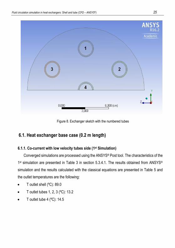
Post program visualization tools are used to get insights on the internal behavior: inside shell
and tubes. The tubes are numbered for their identification, being the central tube the number 4
(Figure 8).
Fluid circulation simulation in heat exchangers: Shell and tube (CFD – ANSYS®) 25
6.1. Heat exchanger base case (0.2 m length)
6.1.1. Co-current with low velocity tubes side (1st Simulation)
Converged simulations are processed using the ANSYS® Post tool. The characteristics of the
1st simulation are presented in Table 3 in section 5.3.4.1. The results obtained from ANSYS®
simulation and the results calculated with the classical equations are presented in Table 5 and
the outlet temperatures are the following:
T outlet shell (ºC): 89.0
T outlet tubes 1, 2, 3 (ºC): 13.2
T outlet tube 4 (ºC): 14.5
Figure 8. Exchanger sketch with the numbered tubes

26 Minella Sivill, Gerard
1st Simulation ANSYS® CLASSICAL Dif. (%)
hs tubes 1,2,3 (W/m2·K) 3670 2230 39
hs tube 4 (W/m2·K) 4137 2222 46
hi tubes 1,2,3 (W/m2·K) 4553 3715 18
hi tube 4 (W/m2·K) 5150 3713 28
ΔPs (Pa) 9.1 11.9 31
ΔPi (Pa) 136.9 102.7 25
The central tube number 4 has higher convection coefficients than the other surrounding
tubes according to ANSYS® simulation (Table 5). Hence the central tube outlet temperature is
higher than for the other tubes. The reason is that its central location confers a higher velocity
gradient and turbulence than for the other tubes where the fluid is slow down in contact with the
shell. The unit symmetry means that all the surrounding tubes have the same results. The
classical equations do not take into account the tube location in the shell and all the tubes are
equivalent.
Table 5. Results and comparison for the 1st Simulation
Figure 9. Velocity Isosurface XY Plane

Fluid circulation simulation in heat exchangers: Shell and tube (CFD – ANSYS®) 27
The difference between ANSYS® results and the Classical results is consequence of the fact
that the classical equations do not take into account the non-stabilized profiles while ANSYS®
considers the microscopic balances in each point of the control volume. For the tube side
convection coefficient, Eq. 3 in section 3.1.2 takes into account the non-stabilized profile, hence
the difference between ANSYS® and classical equations is lower than for the shell side, where
this term has not been developed.
Figure 10 shows the unstabilized profile of temperature for the 2nd and 3rd tube. A ZX Plane
that cuts in the middle of the 2nd and the 3rd tube is created in order to visualize the evolution of
the temperature along the tubes. The stablished range to visualize the variation of the
temperature in the tubes is about 10 ºC and for that reason the shell is all above this temperature
(red colour).
Figure 10. Isometric Temperature Contour 1st Simulation

28 Minella Sivill, Gerard
Figure 11 shows the comparison between the ZX Plane presented in Figure 10 and the
Symmetry Plane in order to visualize the difference between the middle tube and the rest of the
tubes (2nd and 3rd ones, as represented here) as it has been noticed before, outlet temperature
for 4th tube is higher.
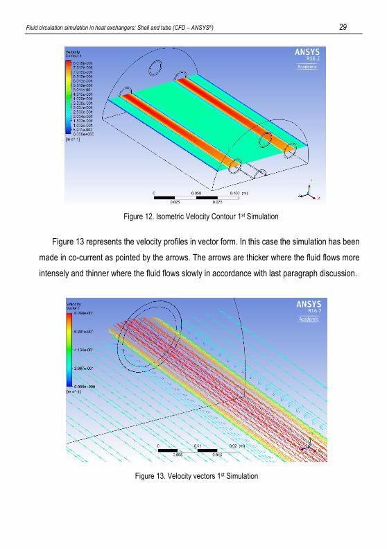
Using the same ZX Plane, the unstabilized profile of velocity is clearly identified. In this case,
all the tubes have the same velocity contour inside, also the 4th tube. Figure 12 shows the plug
flow at the entrance and how it evolves along the tube while the fluid slows down near the walls
and moves faster in the middle. The averaged velocity in a section is constant as the flow rate
must be constant according to the overall mass balance. The fluid flowing inside the shell is also
slowed down by the tubes outer walls.
Figure 11. Temperature Contours 1st Simulation
Fluid circulation simulation in heat exchangers: Shell and tube (CFD – ANSYS®) 29
Figure 13 represents the velocity profiles in vector form. In this case the simulation has been
made in co-current as pointed by the arrows. The arrows are thicker where the fluid flows more
intensely and thinner where the fluid flows slowly in accordance with last paragraph discussion.
Figure 12. Isometric Velocity Contour 1st Simulation
Figure 13. Velocity vectors 1st Simulation

30 Minella Sivill, Gerard
The Figure 14 shows the pressure drop from the inlet to the outlet. Outlet pressure is zero
and specified as boundary condition which means that at the outlet of the heat exchanger there
is the atmospheric pressure. Pressure profiles are the same for all tubes, therefore using the ZX
plane defined previously, pressure drop is observed for tubes 2 and 3. The highest pressure drop
ΔP corresponds to the tubes, and very low ΔP in the shell, which is represented in blue color
(Figure 14).
The heat exchanger is made of 7 tubes and the shell, as described in section 5.1.1, although
for ease of calculation effort, only half of it is plotted, taking advantage of the symmetry tool.
Therefore, ANSYS® calculates as if the whole heat exchanger is present. In Figure 15 the entire
heat exchanger is plotted in order to visualize the variation of pressure in all the tubes, while
Figure 16 illustrates the entire heat exchanger covered by the shell to visualize the temperature
contour.
Figure 14. Isometric Pressure Contour 1st Simulation

Fluid circulation simulation in heat exchangers: Shell and tube (CFD – ANSYS®) 31
6.1.2. Counter - Current with low velocity tubes side (2nd Simulation)
The characteristics of the 2nd simulation are presented in Table 3 in section 5.3.4.1. In this
section is discussed the effect of operating the heat exchanger in counter-current instead of co-
current as in the previous section (6.1.1).
The results obtained from ANSYS® simulation and the results calculated with the classical
equations are presented in Table 6 and the outlet temperatures are the following:
T outlet shell (ºC): 89.0
T outlet tubes 1, 2, 3 (ºC): 13.6
T outlet tube 4 (ºC): 15.1
Figure 15. Pressure contour tubes from whole heat exchanger (Pa)
Figure 16. Temperature contour from whole heat exchanger (ºC)

32 Minella Sivill, Gerard
2nd Simulation ANSYS® CLASSICAL Dif. (%)
hs tubes 1,2,3 (W/m2·K) 3720 2234 40
hs tube 4 (W/m2·K) 4199 2237 47
hi tubes 1,2,3 (W/m2·K) 4627 3733 19
hi tube 4 (W/m2·K) 5233 3699 29
ΔPs (Pa) 9.1 11.9 31
ΔPi (Pa) 136.9 102.5 25
The same tendency observed in the 1st simulation is observed for the 2nd simulation. As far
as the convection coefficients are concerned, the results from ANSYS® turned out to be higher
than the ones calculated with the classical equations of chemical engineering handbooks. The
pressures drops turned out to be the same ones obtained in the 1st Simulation because the only
parameter that has been changed is the flow direction, in this case counter-current. It is also
observed that the outlet temperature of tube 4 keeps being higher than the other tubes because
it shows also higher convection coefficients.
In this 2nd simulation, the fluid flows through the tubes in counter-current, which results in a
higher outlet temperature of the tubes and a slightly lower outlet temperature of the shell. The
convection coefficients turn out to be higher compared with the co-current case with the same
operating parameters. That is, is observed that indeed, working in a counter-current flow a higher
efficiency is achieved. In the case of classical equations a very little variation in the coefficients
and pressure drop is observed because temperature is only relevant for the calculus of
viscosities.
Figure 17 shows the unstabilized profile of temperature in an Isometric Plane. A slight
difference between Figure 10 can be observed due to the major efficiency of counter-current flow
in terms of the outlet temperature.
Table 6. Results and comparison for the 2nd Simulation

Fluid circulation simulation in heat exchangers: Shell and tube (CFD – ANSYS®) 33
A comparison between the plane that cuts the 2nd and 3rd tube with the symmetry plane is
realized in order to visualize the difference of temperatures in Figure 18.
Figure 17. Isometric Temperature Contour 2nd Simulation
Figure 18. Temperature Contours 2nd Simulation

34 Minella Sivill, Gerard
As far as the velocity is concerned, the plot is the same as the 1st simulation, as it has been
mentioned, the only thing that has been varied is the side where the fluid enters in the tubes.
If velocity vectors are represented, it will be observed that the fluid of the shell flows in an
opposite way to the fluid of the tubes because the arrows point out in an opposite direction.
Figure 19. Velocity Contour 2nd Simulation
Figure 20. Velocity vectors 2nd Simulation

Fluid circulation simulation in heat exchangers: Shell and tube (CFD – ANSYS®) 35
Figure 21 shows that the plot of the pressure evolution is the same as the 1st simulation.
6.1.3. Co-Current with fast velocity tubes side (3rd Simulation)
The characteristics of the 3rd simulation are presented in Table 3 in section 5.3.4.1. The aim
of the section is to study the effect of the flow rate inside the tubes.
For this 3rd simulation, the procedure is the same as the previous simulations:
T outlet shell (ºC): 88.9
T outlet tubes 1, 2, 3 (ºC): 12.0
T outlet tube 4 (ºC): 15.0
3rd Simulation ANSYS® CLASSICAL Dif. (%)
hs tubes 1,2,3 (W/m2·K) 6673 2166 68
hs tube 4 (W/m2·K) 7393 2168 71
hi tubes 1,2,3 (W/m2·K) 8523 6657 22
hi tube 4 (W/m2·K) 9484 6666 30
ΔPs (Pa) 9.1 12.2 34
ΔPi (Pa) 467.1 484.6 4
Table 7. Results and comparison for the 3rd Simulation
Figure 21. Pressure Contour 2nd Simulation

36 Minella Sivill, Gerard
The main differences between classical and ANSYS have been already discussed in section
6.1.1 and this section focus on the effect of a flow rate increase inside the tubes. Comparing the
convective coefficients of Table 5 and Table 6 from Table 7 it is stated that now they are higher
than the other previous simulations due to the higher velocity in the tubes from 0.7 m/s to 1.5
m/s. In Table 7 there is a difference between the shell side coefficients of the classical equations
and the ANSYS® ones. The classical equations consider only the shell side for the calculation of
the shell side convective coefficients without considering the interaction with inside the tubes,
which in turn are taken into account in ANSYS® software.
The pressure drop of the tubes has been increase compared with the 1st and 2nd simulation
due to the higher velocity of the fluid.
Figure 22 shows the evolution of the temperature through the tubes in this 3rd simulation. As
a consequence of the increase of velocity, the outlet temperature of tubes that surrounds the
central tube are lower than in previous simulations due to the less time that the fluid is flowing
inside the tubes even though the higher convective coefficients.
Figure 22. Temperature Contour 3rd Simulation

Fluid circulation simulation in heat exchangers: Shell and tube (CFD – ANSYS®) 37
The central tube is 3ºC above the surrounding tubes, which difference is showed in Figure 23.
Velocity contours for the 3rd simulation are showed at Figure 24. It can be observed that the
velocity of tubes is higher than in the shell. The range of the flow velocities has changed
to a larger value so the color of the shell has also changed compared to the 1st and 2nd simulation.
Figure 23. Temperature Contours 3rd Simulation
Figure 24. Velocity Contour 3rd Simulation

38 Minella Sivill, Gerard
There is a significant variation with the pressure in the present simulation compared to the
previous ones. The fact that the fluid flows in a higher velocity inside the tubes produces a higher
pressure drop ΔP between the inlet and the outlet of all the tubes (Figure 25).
6.1.4. Counter-Current with fast velocity tubes side (4th Simulation)
The characteristics of the 4th simulation are presented in Table 3 in section 5.3.4.1. Finally,
the effect of increasing the flow rate is also performed for the counter-current case. For this 4th
simulation, the procedure is the same as the previous simulations:
T outlet shell (ºC): 88.8
T outlet tubes 1, 2, 3 (ºC): 12.2
T outlet tube 4 (ºC): 15.1
Figure 25. Pressure Contour 3rd Simulation

Fluid circulation simulation in heat exchangers: Shell and tube (CFD – ANSYS®) 39
In the last simulation for the 0.2 m length heat exchanger, the same behavior as the previous
simulations is appreciated. There is the difference between ANSYS® and the classical equations
(discussed in section 6.1.1). The fact that operating in counter-current is more efficient than
operating in co-current and also operating in counter-current flow has higher convection
coefficients and outlet temperatures (discussed in section 6.2.2). The different convective
coefficients between ANSYS® and the classical equations in the shell side when the velocity of
the tubes is changed (discussed in section 6.3.3). No parameters have been modified so the
pressure drop is still the same as the 3rd simulation.
An Isometric Plane is presented in Figure 26 to visualize the non-stabilized temperature
profiles for the 4th simulation.
4th Simulation ANSYS® CLASSICAL Dif. (%)
hs tubes 1,2,3 (W/m2·K) 6777 2237 67
hs tube 4 (W/m2·K) 7534 2162 71
hi tubes 1,2,3 (W/m2·K) 8682 6727 23
hi tube 4 (W/m2·K) 9678 6623 32
ΔPs (Pa) 9.1 12.1 33
ΔPi (Pa) 466.1 485.3 4
Table 8. Results and comparison for the 4th Simulation
Figure 26. Temperature Contour 4th Simulation

40 Minella Sivill, Gerard
The different outlets temperatures between the plane that cuts in the middle of the 2nd and
the 3rd tube and the symmetry plane which contains the 4th tube is showed in Figure 27.
The tube number 4 has no yellow colors at the outlet in their walls compared to the other
tubes and it can be also observed that in tubes 2 and 3 at the middle of the tubes they have an
intense blue color while tube number 4 not so much.
The velocity contour has been the same as the 3rd simulation as a consequence that no
parameters have been modified.
Figure 27. Temperature Contours 4th Simulation
Figure 28. Velocity Contour 4th Simulation

Fluid circulation simulation in heat exchangers: Shell and tube (CFD – ANSYS®) 41
A little variation is visualized in the pressure contour compared to the 3rd simulation in Figure
29. That is because the value of the legend has varied hence there is less red color in the inlet
of the tubes, despite this the value for the pressure inlet and the pressure drop ΔP remains equal
to the 3rd simulation.
6.2. Heat exchanger case (0.4 m length)
In this section the four simulations performed for the 0.2 m length heat exchanger base case
are reproduced again with a 0.4 m heat exchanger to determine the effect of the heat exchanger
length.
6.2.1. Co-current with low velocity tubes side (5th Simulation)
The characteristics of the 5th simulation are presented in Table 4 in section 5.3.4.2.
For this 5th simulation, the procedure is the same as the previous simulations but in a 0.4 m
length heat exchanger:
T outlet shell (ºC): 88.5
T outlet tubes 1, 2, 3 (ºC): 15.8
T outlet tube 4 (ºC): 16.5
Figure 29. Pressure Contour 4th Simulation

42 Minella Sivill, Gerard
5th Simulation ANSYS® CLASSICAL Dif. (%)
hs tubes 1,2,3 (W/m2·K) 3527 2228 37
hs tube 4 (W/m2·K) 3887 2219 43
hi tubes 1,2,3 (W/m2·K) 4360 3501 20
hi tube 4 (W/m2·K) 4822 3485 28
ΔPs (Pa) 15.1 23.7 57
ΔPi (Pa) 248.8 209.5 16
Comparing the results obtained in that simulation from the 1st simulation, the conditions were
the same with the difference of the length of the heat exchanger. The outlet temperatures are
higher due to the major length of the heat exchanger. It can be observed that in that case, the
convection coefficients are lower than the 1st simulation. In the classical method, the convection
coefficients are lower due to the term of viscosities. The average of the temperatures is higher in
the tube side and for that reason the convection coefficients get a lower value. In the shell side
is practically the same value because the variation of temperature through the shell is very low.
For the ANSYS® case with a 0.4 m length heat exchanger, the profiles are more stabilized than
for the 0.2 m heat exchanger case. For that reason the velocity gradients are lower and the
turbulence is lower. With a lower turbulence the value of the convection coefficients are lower
too.
The pressure drop has been increased compared with the 1st simulation due to the major
length of the heat exchanger. According to Bernoulli the length has been duplicate and the
pressure drop in the tubes side for the ANSYS® and the classical case has been approximately
duplicate too.
Figure 30 shows the variation of the temperature though the heat exchanger. A large
difference compared with the 0.2 m heat exchanger is observed.
Table 9. Results and comparison for the 5th Simulation

Fluid circulation simulation in heat exchangers: Shell and tube (CFD – ANSYS®) 43
The difference between the tubes number 2 and 3 with the tube number 4 is visualized in
Figure 31.
Figure 30. Temperature Contour 5th Simulation
Figure 31. Temperature Contours 5th Simulation

44 Minella Sivill, Gerard
Figure 32 shows the evolution of velocity inside the tubes.
Figure 33 illustrates the way the velocity is slowed down by the walls and how it increases at
the center while the fluid is flowing through the tubes at the outlet of tubes with a better precision.
Figure 32. Velocity Contour 5th Simulation
Figure 33. Velocity Outlet Contour 5th Simulation

Fluid circulation simulation in heat exchangers: Shell and tube (CFD – ANSYS®) 45
Figure 34 allows to visualize the pressure drop from the inlet to the outlet of the tubes.
6.2.2. Counter-current with low velocity tubes side (6th Simulation)
The characteristics of the 6th simulation are presented in Table 4 in section 5.3.4.2.
For this 6th simulation, the procedure is the same as the previous simulation:
T outlet shell (ºC): 88.4
T outlet tubes 1, 2, 3 (ºC): 16.1
T outlet tube 4 (ºC): 16.8
6th Simulation ANSYS® CLASSICAL Dif. (%)
hs tubes 1,2,3 (W/m2·K) 3577 2228 38
hs tube 4 (W/m2·K) 3940 2224 44
hi tubes 1,2,3 (W/m2·K) 4426 3515 21
hi tube 4 (W/m2·K) 4893 3501 28
ΔPs (Pa) 15.1 23.7 57
ΔPi (Pa) 248.8 206.8 17
Table 10. Results and comparison for the 6th Simulation
Figure 34. Pressure Contour 5th Simulation

46 Minella Sivill, Gerard
The results for that simulation keeps in the line discussed in detail in the previous sections.
The values of the convective coefficients operating in counter-current are higher than the co-
current due to the major efficiency in the 0.4 m heat exchanger case. Comparing the counter-
current convective coefficients with the ones obtained in the 0.2 m heat exchanger they continue
to have a lower value. The pressure drop values only have changed a few in the classical model
due to the little variation of temperature in the viscosity term.
A little difference in the outlet temperature can be observed compared to the co-current 0.4
m case.
Comparing the tube number 4 with tubes number 2 and 3, the difference is lower in terms of
visualization because the difference is about 0.8 ºC. In a more detailed analysis a small difference
can be observed in terms of colors defining the temperature inside the tubes (Figure 36).
Figure 35. Temperature Contour 6th Simulation

Fluid circulation simulation in heat exchangers: Shell and tube (CFD – ANSYS®) 47
The following figures illustrate that velocity and pressure maintain in the line as the previous
simulations (Figure 37 and Figure 38, respectively).
Figure 36. Temperature Contours 6th Simulation
Figure 37. Velocity Contour 6th Simulation

48 Minella Sivill, Gerard
6.2.3. Co-current with fast velocity tubes side (7th Simulation)
The characteristics of the 7th simulation are presented in Table 4 in section 5.3.4.2.
For this 7th simulation, the procedure is the same as the previous simulation:
T outlet shell (ºC): 88.0
T outlet tubes 1, 2, 3 (ºC): 13.4
T outlet tube 4 (ºC): 15.3
7th Simulation ANSYS® CLASSICAL Dif. (%)
hs tubes 1,2,3 (W/m2·K) 6453 2170 66
hs tube 4 (W/m2·K) 7010 2166 69
hi tubes 1,2,3 (W/m2·K) 8192 6274 23
hi tube 4 (W/m2·K) 8953 6241 30
ΔPs (Pa) 15.1 23.6 56
ΔPi (Pa) 849.6 945.2 11
Table 11. Results and comparison for the 7th Simulation
Figure 38. Pressure Contour 6th Simulation

Fluid circulation simulation in heat exchangers: Shell and tube (CFD – ANSYS®) 49
The results for this simulation keeps in the line discussed in detail in the other previous
sections.
Table 11 shows the results for the simulation. The rate inside the tubes is 1.5 m/s that
provides a higher pressure drop together with the increase of the length of the heat exchanger.
In the shell side all the parameters have been kept equal from all the simulations, only the length
of the heat exchanger produces a bit higher pressure drop compared to the simulations of the
0.2 m heat exchanger.
The values for the outlet temperatures are lower than the 0.7 m/s co-current and counter-
current cases in consequence of the less time the fluid is flowing inside the tubes.
Figure 39 can show this phenomena, the fluid is not heated as much as the other simulations
for the 0.4 m heat exchanger.
The difference of about 2 ºC between the central tube and surrounding tubes is illustrated in
Figure 40.
Figure 39. Temperature Contour 7th Simulation

50 Minella Sivill, Gerard
Velocity contour is showed in Figure 41 with the same observations discussed in previous
simulations.
Figure 40. Temperature Contours 7th Simulation
Figure 41. Velocity Contour 7th Simulation

Fluid circulation simulation in heat exchangers: Shell and tube (CFD – ANSYS®) 51
There is a clear difference between all the simulations performed and this one in particular.
The pressure drop has been the highest of all the simulations due to the velocity inside the tubes
and the length of the heat exchanger. Figure 42 shows the values for the pressure from the inlet
to the outlet.
6.2.4. Counter-Current with fast velocity tubes side (8th Simulation)
The characteristics of the 8th simulation are presented in Table 12 in section 5.3.4.2.
For this 8th simulation, the procedure is the same as the previous simulation:
T outlet shell (ºC): 87.9
T outlet tubes 1, 2, 3 (ºC): 13.6
T outlet tube 4 (ºC): 15.7
Figure 42. Pressure Contour 7th Simulation
52 Minella Sivill, Gerard
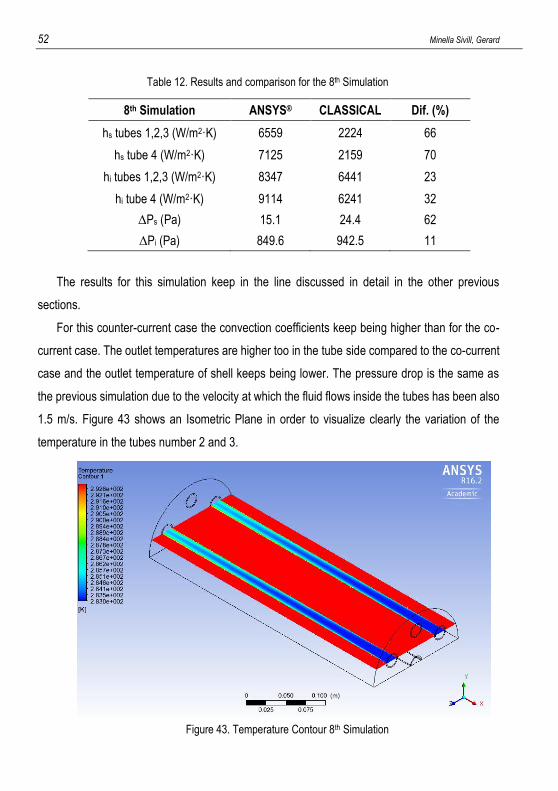
8th Simulation ANSYS® CLASSICAL Dif. (%)
hs tubes 1,2,3 (W/m2·K) 6559 2224 66
hs tube 4 (W/m2·K) 7125 2159 70
hi tubes 1,2,3 (W/m2·K) 8347 6441 23
hi tube 4 (W/m2·K) 9114 6241 32
ΔPs (Pa) 15.1 24.4 62
ΔPi (Pa) 849.6 942.5 11
The results for this simulation keep in the line discussed in detail in the other previous
sections.
For this counter-current case the convection coefficients keep being higher than for the co-
current case. The outlet temperatures are higher too in the tube side compared to the co-current
case and the outlet temperature of shell keeps being lower. The pressure drop is the same as
the previous simulation due to the velocity at which the fluid flows inside the tubes has been also
1.5 m/s. Figure 43 shows an Isometric Plane in order to visualize clearly the variation of the
temperature in the tubes number 2 and 3.
Table 12. Results and comparison for the 8th Simulation
Figure 43. Temperature Contour 8th Simulation

Fluid circulation simulation in heat exchangers: Shell and tube (CFD – ANSYS®) 53
The different evolution of the temperatures for tubes number 2 and 3 compared with the tube
number 4 is presented in Figure 44 in a contour plot to visualize the variation of the colors.
Velocity contour is showed in Figure 45 with the same observations discussed in previous
simulations.
Figure 44. Temperature Contours 8th Simulation
Figure 45. Velocity Contour 8th Simulation
54 Minella Sivill, Gerard
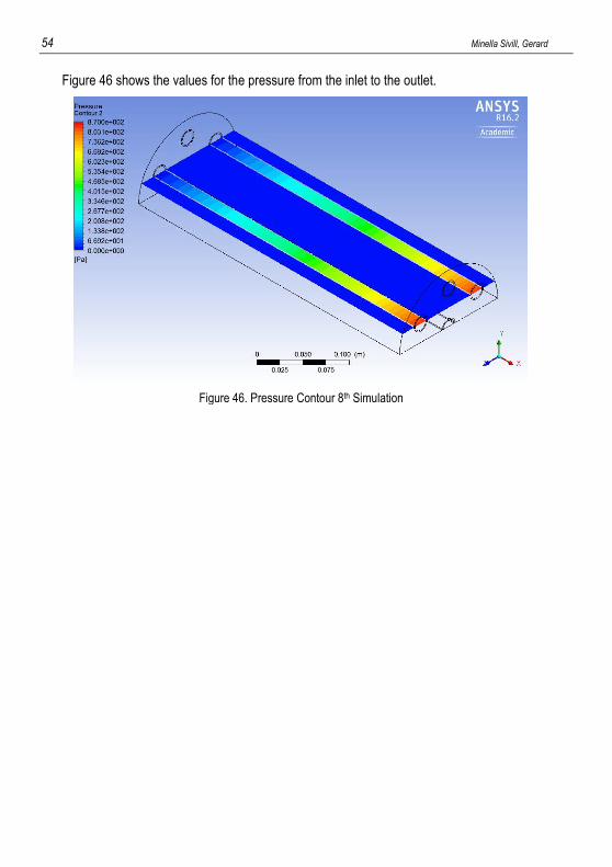
Figure 46 shows the values for the pressure from the inlet to the outlet.
Figure 46. Pressure Contour 8th Simulation
Fluid circulation simulation in heat exchangers: Shell and tube (CFD – ANSYS®) 55
7. CONCLUSIONS
ANSYS® software allows to have a virtual laboratory able to save experimental
laboratory time. The results have a rather good precision and parameters are easily
assessed.
ANSYS® takes into account the non-stabilized profiles while the majority of classical
equations are only developed for the stabilized conditions.
ANSYS® takes into account the interaction between the shell side and the tubes
side for the convection coefficients. Without changing any parameter for the shell
side, the convection coefficients have increased also in the shell side when the flow
rate inside the tubes increases. The classical equations calculate the convection
coefficients for the shell independently of the tubes.
It can be observed that effectively operating in counter-current is more efficient than
operating in co-current.
ANSYS® takes into account the position of tubes inside the shell and how the
turbulence can affect the convection coefficients. This aspect is not considered in
classical equations.
Working with ANSYS® a numeric visualization at microscopic level is provided with
the Post-Processing program once the solution of the balances has been
converged. Different contour plots such as temperature, velocity and pressure are
represented for the shell and tube heat exchanger.


Fluid circulation simulation in heat exchangers: Shell and tube (CFD – ANSYS®) 57
8. REFERENCES AND NOTES
ANSYS® Fluent 16.2 in Workbench User’s Guide. ANSYS, Inc. License Manager Release 16.2, 2016
ANSYS® Meshing User’s Guide. ANSYS, Inc. License Manager Release 16.2, 2016
ANSYS® Fluent Theory Guide. ANSYS, Inc. License Manager Release 16.2, 2016
Alimoradi, A.; Veysi F. Prediction of heat transfer coefficients of shell and coiled tube heat exchangers using
numerical method and experimental validation. International Journal of Thermal Sciences. 2016, 107, 196 –
208
Dong, Q.W.; Wang, Y.Q.; Liu, M.S. Numerical and experimental investigation of shell side characteristics for
RODbaffle heat exchanger. Applied Thermal Engineering. 2007, 28, 651 - 660
Levenspiel, O. Flujo de fluidos e intercambio de calor. Barcelona: Reverté. 1993
Llorens, J. Apunts de Fenòmens de Transport. Universitat de Barcelona. 2016
Pal, E.; Kumar, I.; Joshi, J.B.; Maheshwari, N.K. CFD Simulations of shell side flow in a shell and tube type
heat exchanger with and without baffles. Chemical Engineering Science. 2016, 143, 314 - 340
Perry, R.H.; Green, D.W. Perry’s Chemical Engineers’ Handbook, 8th Edition. McGraw-Hill: United States of
America. 2008
Serth, R.W. Process heat transfer, principles and applications. 1st Edition. Burlington: Elsevier. 2007
Sinnott, R.K. Chemical Engineering Design. 4th Edition. Burlington: Elsevier. 2008, 6
Wen, J.; Yang, H.; Jian, G.; Tong, X.; Li, K.; Wang, S. Energy and cost optimization of shell and tube heat
exchanger with helical baffles using Kriging metamodel base don MOGA. International Journal of Heat and
Mass Transfer. 2016, 98, 29 - 39
Zhang, M.; Meng, F.; Geng, Z. CFD simulation on shell and tube heat exchangers with small angle helical
baffles. Chemical Science Engineering. 2015, 9(2), 183 – 193
Zhou, G.; Xiao, J.; Zhu, L.; Wang, J.; Tu, S. A numerical study on the shell side turbulent heat transfer
enhancement of shell and tube heat exchanger with trefoil-hole baffles. 7th International Conference on
Applied Energy. 2015, 75, 3174 - 3179


Fluid circulation simulation in heat exchangers: Shell and tube (CFD – ANSYS®) 59
9. ACRONYMS
Nu Nusselt number
hs Convection coefficient for the shell side (W/m2·K)
de Equivalent diameter (m)
kf Fluid thermal conductivity (W/m·K)
jh Heat transfer factor
Re Reynolds number
Pr Prandtl number
µ Fluid viscosity at the bulk fluid temperature (Pa·s)
µw Fluid viscosity at the wall (Pa·s)
ΔPs Pressure drop for the shell side (Pa)
jf Friction factor
Ds Shell diameter (m)
L Tube length (m)
lB Baffle spacing (m)
ρ Density (kg/m3)
us Fluid velocity of the shell side (m/s)
ut Fluid velocity of the tube side (m/s)
hi Convection coefficient for the tube side (W/m2·K)
ΔPi Pressure drop for the tube side (Pa)
di Inlet diameter (m)
�⃗� The velocity vector (m/s)
E The total energy per unit mass (J)
P The static pressure (Pa)

60 Minella Sivill, Gerard
Jj Flux mass (kg/s)
𝑔 Gravitational force (N)
𝜏̿ The stress tensor
𝐹 External body forces (N)
I The unit tensor (matrix identity)
k Turbulence kinetic energy (J/kg)
ε Turbulence dissipation rate (J/kg·s)
T Temperature (ºC)
σε Turbulent Prandtl number for ε
σk Turbulent Prandtl number for k