Embed Size (px)
Citation preview
Treball Final de Grau
Tutors
Dra. Alexandra E. Bonet Ruiz
Dr. Ricardo Torres Castillo
Secció Departamental d’Enginyeria Química
ANSYS Fluent simulation of a solar chimney
Simulació d’una xemeneia solar en ANSYS Fluent
Ricardo Moya Chamizo
June, 2017


Aquesta obra està subjecta a la llicència de:
Reconeixement–NoComercial-SenseObraDerivada
http://creativecommons.org/licenses/by-nc-nd/3.0/es/


En primer lloc, agrair als meus pares, i companys de classe tota la confiança, ànims i suport
absoluts que m’han prestat, sense ells tot hauria sigut molt complex.
En segon lloc, dono les gracies als meus tutors, Ricard Torres i Alexandra Bonet, per les
ajudes indiscutibles rebudes per part seva, tant referides al treball com consells aleatoris de tots
els camps d’enginyeria, i sobretot pel seu comportament humà.
Finalment dono les gracies a la resta del professorat, per tot el que he après gracies a les
seves classes i per conseqüència la confiança personal que he guanyat en vers a la vida laboral.


REPORT


Study of a Solar Chimney using CFD (ANSYS®) 9
CONTENTS
1. SUMMARY. . . . . . . . . . . . . . . . . . . . . . . . . . . . . . . . . . . . . . . . . . . . . . . . . . . . . . . . . . . . . . . . . . . . . . . . .10
2. RESUM. . . . . . . . . . . . . . . . . . . . . . . . . . . . . . . . . . . . . . . . . . . . . . . . . . . . . . . . . . . . . . . . . . . .11
3. INTRODUCTION. . . . . . . . . . . . . . . . . . . . . . . . . . . . . . . . . . . . . . . . . . . . . . . . . . . . . . . . . . . . . . 13
3.1. State of the art. . . . . . . . . . . . . . . . . . . . . . . . . . . . . . . . . . . . . . . . . . . . . . . . . . . . . . . . . . . . . . .16
3.2. Project which the simulation is based on. . . . . . . . . . . . . . . . . . . . . . . . . . . . . . . . . . . . . .19
4. OBJECTIVES. . . . . . . . . . . . . . . . . . . . . . . . . . . . . . . . . . . . . . . . . . . . . . . . . . . . . . . . . . . . . . . 21
5. MATERIALS AND METHODS: USING ANSYS®. . . . . . . . . . . . . . . . . . . . . . . . . . . . . . . . . . . . . . . . 22
5.1 Geometry design. . . . . . . . . . . . . . . . . . . . . . . . . . . . . . . . . . . . . . . . . . . . . . . . . . . . . . . . . . . . 23
5.2 Mesh generation. . . . . . . . . . . . . . . . . . . . . . . . . . . . . . . . . . . . . . . . . . . . . . . . . . . . . . . . . . . . .28
5.3 Simulation setup. . . . . . . . . . . . . . . . . . . . . . . . . . . . . . . . . . . . . . . . . . . . . . . . . . . . . . . . . . . ..32
6. RESULTS AND DISCUSSION. . . . . . . . . . . . . . . . . . . . . . . . . . . . . . . . . . . . . . . . . . . . . . . . . . . . . 36
6.1. Temperature contours, graphics and integrals. . . . . . . . . . . . . . . . . . . . . . . . . . . . . . . .. 37
6.2. Density contours, graphics and integrals. . . . . . . . . . . . . . . . . . . . . . . . . . . . . . . . . . . . . 43
6.3. Velocity contours, graphics and integrals. . . . . . . . . . . . . . . . . . . . . . . . . . . . . . . . . . . . . 47
7. CONCLUSIONS. . . . . . . . . . . . . . . . . . . . . . . . . . . . . . . . . . . . . . . . . . . . . . . . . . . . . . . . . . . . . . .56
8. RECOMMENDATIONS. . . . . . . . . . . . . . . . . . . . . . . . . . . . . . . . . . . . . . . . . . . . . . . . . . . . . . . . . .57
9. FUTURE WORK. . . . . . . . . . . . . . . . . . . . . . . . . . . . . . . . . . . . . . . . . . . . . . . . . . . . . . . . . . . . . . 58
10. REFERENCES AND NOTES. . . . . . . . . . . . . . . . . . . . . . . . . . . . . . . . . . . . . . . . . . . . . . . . . . . . . . . . . . .59
11. NOMENCLATURE & SYMBOLS. . . . . . . . . . . . . . . . . . . . . . . . . . . . . . . . . . . . . . . . . . . . . . . . . . . . . . . .60

10 Moya Chamizo Ricardo
1. SUMMARY
This final degree project aims to model a chimney to incorporate it in a future work, which is a whole solar chimney model, also to compare temperature data obtained from an experimental pilot plant (literature) with temperature data obtained from two ANSYS® simulated models. To make a comparison of the results, there will be a study of temperature at different heights marked as 10#, 11# and 12#, matching the available experimental points. The simulation used models are: model with atmosphere, to obtain the indoor and outdoor data as accurate as possible, and a model without atmosphere. Once the results are obtained and compared to experimental data, the both simulated models would be compared between them. Finally, there will be studies of temperature, density, velocity and turbulence for both.
There is detailed explanation of each ANSYS® module. The explained modules are the Geometry design, Mesh Generation and Model Setup of Fluent, being this last one to quantify and export results, emphasizing in distributions, profiles, contours and values of temperature, density and velocity throughout the system. In the Geometry Design, the chosen geometry was 2D, in order to make it easier to compute.
The solar chimney dimensions are: a cylinder with, 8 m high and 30 cm diameter for both models. In the atmosphere model, the atmosphere dimensions surrounding chimney cylinder are 160 meters high and 3 meters in width with respect to the center of the chimney. For both models, the outdoor temperature and pressure are 305.5 K and 101,325 Pa respectively. The chimney inlet temperature is 322.4 K.
The pictures were obtained as contour and vector formats. The distributions of temperature, density, velocity and turbulence throughout the system are shown. The graphical profiles of temperature, density and speed at different heights and, the numerical data tables of temperature, density, velocity and Reynolds, are shown for both models too. The obtained results of the simulation, have a similarity for the atmosphere model and the model without atmosphere of 99.7% and 99.5% respectively between them and the experimental data.
The results of temperature in each of the predetermined heights are nearly identical to the experimental data in both simulations.
The atmosphere model reproduces more realistic results than the model without atmosphere.
Given that the goal of the study is to compare the results with a real case, confirms the fact that the two models give acceptable and similar values.
If there is an interest in designing a new chimney, it is recommended the implementation of the atmosphere model.
Given the results of comparing models, it is verified that all the results as density, speed, Reynolds and heat transfer coefficients are correct.

Study of a Solar Chimney using CFD (ANSYS®) 11
2. RESUM
Aquest treball final de grau pretén modelitzar una xemeneia per adaptar-la posteriorment
a un model complet d’una xemeneia solar i també comparar les dades de temperatura obtingudes
d’un cas experimental (bibliogràfic) amb les dades de temperatura obtingudes en els dos models
simulats amb el programa ANSYS®. Per tal de comparar els resultats, es realitzarà l’estudi de
temperatura a les diferents altures predeterminades i senyalitzades com a 10#, 11# i 12#,
utilitzant un model amb atmosfera inclosa, per aconseguir les dades de l’interior i l’exterior de la
forma més acurada possible i, un model sense incloure l’atmosfera envoltant. Un cop obtinguts i
comparats els resultats amb les dades experimentals, es compararan els dos models simulats
entre ells, i finalment, es realitzaran estudis de temperatura, densitat, velocitat i turbulència per
ambdós.
S’ha realitzat una explicació detallada de cada mòdul de l’ANSYS®. Els mòduls explicats
han sigut el Geometry design, el Mesh generation i el Model Setup del Fluent, havent sigut aquest
últim programat per quantificar i exportar resultats, emfatitzant en les distribucions, perfils,
contorns y valors de temperatura, densitat i velocitat en tot el sistema d’estudi. En el Geometry
Design es va optar per realitzar l’estudi per pura geometria en 2D, per facilitar la velocitat de
computació. En el Mesh generation es va optar per fer la malla de la forma mes complexa,
manualment. En el Model Setup del Fluent s’han trobat dificultats amb els “under-relaxation
factors”, per motiu del temps de computació requerit.
Les característiques de la xemeneia solar son: un cilindre de 8 m d’altura i 30 cm de
diàmetre per ambdós models, les dimensions de la atmosfera circumdant en el cas del model
amb atmosfera son 160 m d’altura i 3 m d’amplada respecte del centre de la xemeneia. Per als
dos models, la temperatura exterior és de 305,5 K, la pressió atmosfèrica és de 101.325 Pa i, a
l’entrada de la xemeneia la temperatura d’entrada és de 322,4 K.
S’han obtingut imatges en format “contours” i vectorials de les distribucions de
temperatura, densitat, velocitat i turbulència en tot el sistema, gràfics dels perfils de temperatura,
densitat i velocitat a diferents altures preestablertes, i taules de dades d’integrals realitzades a
les diferents altures preestablertes, amb resultats numèrics de temperatura, densitat, velocitat i
Reynolds, per ambdós models. Els resultats obtinguts per la simulació tenen una similitud amb
les dades experimentals, pels models amb atmosfera i sense atmosfera de 99,7% i 99,5%
respectivament.

12 Moya Chamizo Ricardo
Els resultats de temperatura en cadascuna de les altures predeterminades son
pràcticament idèntics a les dades experimentals en les dues simulacions. Es pot observar com
el model amb atmosfera reprodueix resultats més realistes que els del model sense atmosfera.
En el cas de que el que interessa sigui dissenyar una nova xemeneia, es recomana la
realització del model amb atmosfera. Tenint en compte els resultats de temperatura y pressió
obtinguts en la comparació de models, es verifica que tots els resultats obtinguts, com la densitat,
la velocitat, el Reynolds i els coeficients de transmissió de calor son reproduïbles i de confiança.

Study of a Solar Chimney using CFD (ANSYS®) 13
3. INTRODUCTION
The concept of Solar chimney power technology was first conceived in 1931 by Hanns
Gunther, and was proven with the successful operation of a pilot plant constructed in Manzanares
(Spain) in the early 1980s. The natural ventilation is the best way to improve the indoor thermal
and breeze comfort and to reduce the energy consumption that is used in artificial ventilation
systems. A solar chimney system uses solar radiation to heat the air inside a control volume,
thereby converting the thermal energy into kinetic energy.
The increase in world population and the improvement of living standards led to a growing
demand for electricity. The limited availability of fossil fuels and environmental pollution caused
by them, push the development of innovative technologies to produce electricity from renewable
energy sources. With a view to sustainable development, therefore, the energy future must have
as protagonists renewable sources (solar, geothermal, wind, etc.), which are not exhausted and
have no environmental impact because they do not produce greenhouse gases.
In building constructions after the international energy crisis in 1973, the energy required
for heating and cooling of buildings was approximately 40% of the total world energy consumption.
The indoor environment for summer is normally obtained by air conditioning or ventilation
including mechanical ventilation and natural ventilation (N. Pasumarthi, 1998). Natural ventilation
not only can save energy and life cycle costs, but also can alleviate the environmental charge
from the products used in energy production. There is not only one purpose, but the first one is to
replace the air conditioning systems in certain regions. Modern society, is characterized by high
civilization level and advanced accommodations, involving heating supply for the severe winter
and air conditioning for warm summer. The annual summary report of International Energy
Agency (IEA) shows that for the well-insulated office buildings, with a well-controlled natural
ventilation system can reduce more than 50% of energy requirement.
A solar chimney is essentially divided into two parts, one is the solar air heater (collector)
and the second one is the chimney, as shown in Figure 1 and 2. Two configurations usually used
are: vertical solar chimney with vertical absorber geometry, and roof solar chimney. For the
vertical configuration, vertical glass or steel is used to gain solar heat (there are also mechanical
issues because of the wind, therefore the material must be resistant). The temperature difference
between vertical glass duct and interior room produces a pressure difference. An interior air will
go out through inlet because of this pressure difference. The temperature difference is a
determining factor of performance of solar chimney. Designing a solar chimney includes height,
14 Moya Chamizo Ricardo
width and depth of cavity, type of glazing, type of absorber, etc. Besides these system parameters,
other factors such as the location, climate, and orientation can also affect its performance.
The present study considered the same structural parameters as (Zhou et al. 2007) did
use in their real and physic Solar chimney. Their project which was published as experimental
and theoretical results, is going to be used in order to make a comparison between their results
and the ones obtained by (ANSYS Fluent User's Guide) Fluent simulator. The Schematic diagram
of the proposed model with the collector drown for a better understand is shown in Figure 2.
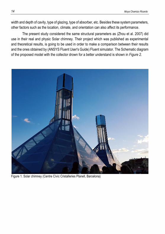
Figure 1. Solar chimney (Centre Cívic Cristalleries Planell, Barcelona)

Study of a Solar Chimney using CFD (ANSYS®) 15
Figure 2. Diagram of solar chimney proposed model (with collector and red axis-symmetric centerline)
16 Moya Chamizo Ricardo
3.1. STATE OF THE ART
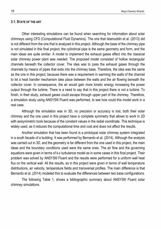
Other interesting simulations can be found when searching for information about solar
chimneys using CFD (Computational Fluid Dynamics). The one that Islamuddin et al. (2013) did
is not different from the one that is analyzed in this project. Although the base of the chimney pipe
is not simulated in this final project, the cylindrical pipe is the same geometry and form, and the
main ideas are quite similar. A model to implement the exhaust gases effect into the classical
solar chimney power plant was needed. The proposed model consisted of hollow rectangular
channels beneath the collector cover. The idea was to pass the exhaust gases through the
channels by means of pipes that exits into the chimney base. Therefore, the idea was the same
as the one in this project, because there was a requirement in warming the walls of the channel
to let a heat transfer mechanism take place between the walls and the air flowing beneath the
collector cover. In consequence, the air would gain more kinetic energy increasing the power
output through the turbine. There is a need to say that in this project there is not a turbine. To
finish, in their study, exhaust gases could escape through upper part of the chimney. Therefore,
a simulation study using ANSYS® Fluent was performed, to see how could this model work in a
real case.
Although the simulation was in 3D, no precision or accuracy is lost, both their solar
chimney and the one used in this project have a complete symmetry that allows to work in 2D
with axisymmetric tools because of the constant values in the radial coordinate. This technique is
widely used, as it reduces the computational time and cost and does not affect the results.
Another simulation that has been found is a prototypal solar chimney system integrated
in a south facade of a building. It was performed by Bernardo et al. (2014). Although the analysis
was carried out in 3D, and the geometry is far different from the one used in this project, the main
ideas and the boundary conditions used were the same ones. The air flow and the governing
equations were given in terms of k-ε turbulence model as in some cases in this final project. Their
problem was solved by ANSYS® Fluent and the results were performed for a uniform wall heat
flux on the vertical wall. All the results, as in this project were given in terms of wall temperature
distributions, air velocity, temperature fields and transversal profiles. The main difference is that
Bernardo et al. (2014) modeled this to evaluate the differences between two base configurations.
The following Table 1, shows a bibliographic summary about ANSYS® Fluent solar
chimney simulations.

Study of a Solar Chimney using CFD (ANSYS®) 17
Table 1. Summary table of ANSYS® simulations with properties and generalities. hs (heath transfer
coefficient), Eext (external emissivity), K-∈ (turbulent method). In green, this project.
References Real
format
Format
and model
Outlet
boundary
conditions
Inlet
boundary
conditions
Chimney
walls
boundary
conditions
Collector
boundary
conditions
Atmosphere
walls
boundary
conditions
Atmosphere
Interior
Islamuddin et al. 2013
3D cylinder + Conic Collector
3D, unavailable
Top chimney zone (circular). Pressure outlet
Bottom chimney zone (circular). Mass inlet
unavailable unavailable none none
Bernardo et al. 2014
3D squared
3D, Turbulent
K-∈
Top chimney zone (square). Pressure outlet
Bottom chimney zone (square). Pressure inlet
Heat flux none none none
Sudprasert et al. 2016
3D cylinder
2D, Turbulent
K-∈
Top left chimney zone (circular). Pressure outlet
Bottom left chimney zone (circular). Pressure inlet
Constant temperature (∞ heat transfer coefficient)
none none none
Hu et al. 2017 3D cone + Conic Collector
2D, Turbulent
K-∈
Top chimney zone (circular). Pressure outlet
Bottom chimney zone (circular). Pressure inlet
Adiabatic wall
Mixed wall: T, hs, Eext
none none
Degree final project
3D cylinder
2D, Turbulent
K-∈
Top chimney zone (circular). Pressure outlet
Bottom chimney zone (circular). Velocity inlet
Convection/ conduction/ convection
none Constant temperature
Real gas
Degree final project
3D cylinder
2D, Turbulent
K-∈
Top chimney zone (circular). Pressure outlet
Bottom chimney zone (circular). Velocity inlet
Constant temperature (∞ heat transfer coefficient)
none none none
In the simulation of Bernardo et al. (2014), all the thermophilically fluid properties were
assumed to be invariant except the density, which is different from this project where the density
and the viscosity are both variant. The compression work, viscous dissipation and radiative
transport were negligibly small, in this project all those are used as not negligible to make the

18 Moya Chamizo Ricardo
study more realistic. They considered the steady, turbulent, 3D natural convection flow in a solar
chimney as shown in Figures 3 and 4.
Figure 3. Geometry configuration Figure 4. Temperature field on vertical surface

Study of a Solar Chimney using CFD (ANSYS®) 19
3.2. PROJECT WHICH THE SIMULATION IS BASED ON
The previously mentioned work of Zhou et al. (2007), is an experimental study of
temperature field in a solar chimney power setup. This final project is based in their work.
Therefore, is important to be said that all the parameters that are used in this project are extracted
from the mentioned work in order to check if the ANSYS® Fluent is capable to make the simulation
and deliver the same results.
In order to perform a detailed investigation into the measured temperature field in solar
chimney power system, a pilot experimental setup was built as shown in Figure 5, consisted in a
10 m diameter air collector, 8 m chimney height and 30 cm chimney diameter, it was built in HUST,
China. It is why in this project the 8 m tall chimney is defined as the cylinder, but there is no
collector defined, because all the experimental and numeric information given is at the chimney
inlet and outlet and there is not anything explained about materials, thickness and composition of
the base collector. The chimney was built on the roof of a building, to avoid the shadows of
buildings on the collector.
Figure 5. Pilot experimental setup (Zhou et al. 2007)
The cylinder of the schematic diagram shown in Figure 6, is going to be the pattern for
this one, in fact the tags shown in Figure 6 (#9, 10#, 11#, 12#) are the nomenclature used in the
present final project. The #9 is going to be the fluid flow entrance (inlet) of the pipe, and the 10#,
11#, 12# are going to be diferent heighs where the wall temperature, air temperature, density and
velocity distributions inside and outside the chimney, as well as temperature, density and velocity
fields and transversal profiles are going to be shown. Also, another experimental performance

20 Moya Chamizo Ricardo
with a prototype solar chimney was checked (Kulunk, 1985), this was done to check the similarity
between them in order to understand better the results.
To check if the values of velocity are the correct ones, and therefore the simulation is well
done, the temperature surface integral in each height must have the same numeric value as (Zhou
et al. 2007), with the minimum error possible. (see Figure 7).
Figure 6. Schematic diagram of proposed model
The boundary conditions that have been extracted from the Zhou et al. (2007) project
would be the following ones: ambient air 305.5 K, velocity inlet 2.13 m/s, and pressure outlet
1 atm.
Figure 7. Distribution of air temperatures at different heights in solar chimney on a typical warm
day (ambient temperature; 305.5 K, updraft velocity in the chimney; 2.13 m/s)
Study of a Solar Chimney using CFD (ANSYS®) 21
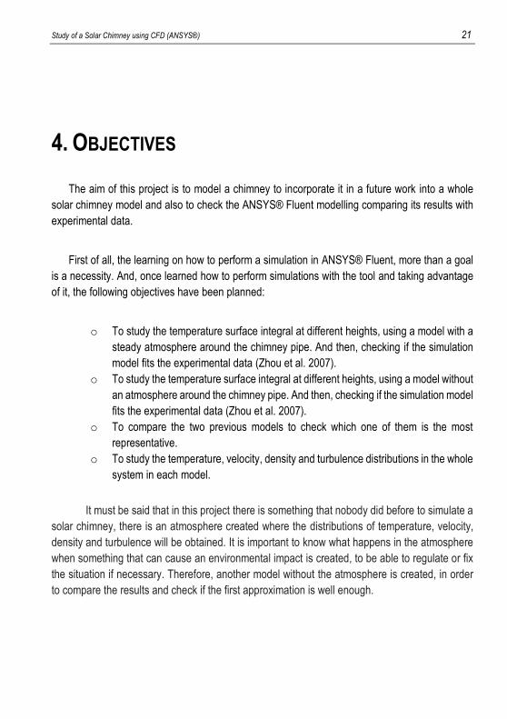
4. OBJECTIVES
The aim of this project is to model a chimney to incorporate it in a future work into a whole
solar chimney model and also to check the ANSYS® Fluent modelling comparing its results with
experimental data.
First of all, the learning on how to perform a simulation in ANSYS® Fluent, more than a goal
is a necessity. And, once learned how to perform simulations with the tool and taking advantage
of it, the following objectives have been planned:
o To study the temperature surface integral at different heights, using a model with a
steady atmosphere around the chimney pipe. And then, checking if the simulation
model fits the experimental data (Zhou et al. 2007).
o To study the temperature surface integral at different heights, using a model without
an atmosphere around the chimney pipe. And then, checking if the simulation model
fits the experimental data (Zhou et al. 2007).
o To compare the two previous models to check which one of them is the most
representative.
o To study the temperature, velocity, density and turbulence distributions in the whole
system in each model.
It must be said that in this project there is something that nobody did before to simulate a
solar chimney, there is an atmosphere created where the distributions of temperature, velocity,
density and turbulence will be obtained. It is important to know what happens in the atmosphere
when something that can cause an environmental impact is created, to be able to regulate or fix
the situation if necessary. Therefore, another model without the atmosphere is created, in order
to compare the results and check if the first approximation is well enough.

22 Moya Chamizo Ricardo
5. MATERIALS AND METHODS: USING ANSYS®
This simulation is going to be done by computational fluid dynamics modelling, using
ANSYS® Fluent commercial software.
Computational fluid dynamics (CFD), is the cheaper way in designing and running simulations
and experiments, and there is no need to create or build the pilot plant. The cost of pilot plant
building and repeating the process until the desired result is quite large.
Selecting the appropriate models is the way that is going to give the correct results, because
there is no precision or accuracy if the global model is not well done. In the following subsections,
the chosen models are explained, and reasons why they are used are given.
The ANSYS® commercial software provides access to several modules that allow to simulate
a high number of scenarios focusing in many different engineering cases. The Fluent is one of
those ANSYS® modules, and its characteristics and sub-models are suitable for the solar
chimney that is going to be simulated.
A brief description of how does the software program work is going to be explained in order
to understand better the work, also it is going to be explained what does the user need to perform
a simulation.
Each step is going to be explained to perform a successfully simulation. Focusing on the
mathematical models and on the boundary conditions formation setup.
The previous steps that must be completed to perform a simulation are the following:
1- Geometry design
2- Mesh generation
3- Models set up
Study of a Solar Chimney using CFD (ANSYS®) 23
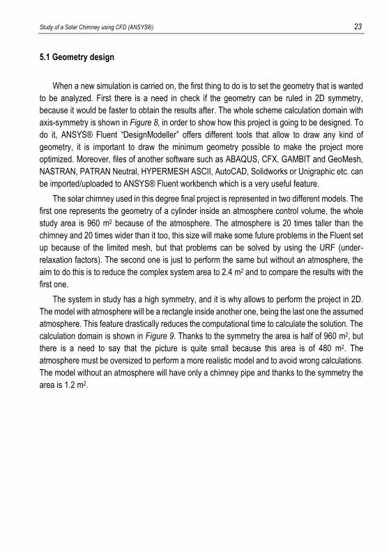
5.1 Geometry design
When a new simulation is carried on, the first thing to do is to set the geometry that is wanted
to be analyzed. First there is a need in check if the geometry can be ruled in 2D symmetry,
because it would be faster to obtain the results after. The whole scheme calculation domain with
axis-symmetry is shown in Figure 8, in order to show how this project is going to be designed. To
do it, ANSYS® Fluent “DesignModeller” offers different tools that allow to draw any kind of
geometry, it is important to draw the minimum geometry possible to make the project more
optimized. Moreover, files of another software such as ABAQUS, CFX, GAMBIT and GeoMesh,
NASTRAN, PATRAN Neutral, HYPERMESH ASCII, AutoCAD, Solidworks or Unigraphic etc. can
be imported/uploaded to ANSYS® Fluent workbench which is a very useful feature.
The solar chimney used in this degree final project is represented in two different models. The
first one represents the geometry of a cylinder inside an atmosphere control volume, the whole
study area is 960 m2 because of the atmosphere. The atmosphere is 20 times taller than the
chimney and 20 times wider than it too, this size will make some future problems in the Fluent set
up because of the limited mesh, but that problems can be solved by using the URF (under-
relaxation factors). The second one is just to perform the same but without an atmosphere, the
aim to do this is to reduce the complex system area to 2.4 m2 and to compare the results with the
first one.
The system in study has a high symmetry, and it is why allows to perform the project in 2D.
The model with atmosphere will be a rectangle inside another one, being the last one the assumed
atmosphere. This feature drastically reduces the computational time to calculate the solution. The
calculation domain is shown in Figure 9. Thanks to the symmetry the area is half of 960 m2, but
there is a need to say that the picture is quite small because this area is of 480 m2. The
atmosphere must be oversized to perform a more realistic model and to avoid wrong calculations.
The model without an atmosphere will have only a chimney pipe and thanks to the symmetry the
area is 1.2 m2.

24 Moya Chamizo Ricardo
Figure 8. Whole scheme calculation domain with axis-symmetry in red
Study of a Solar Chimney using CFD (ANSYS®) 25
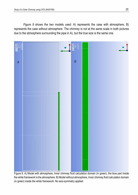
Figure 9 shows the two models used: A) represents the case with atmosphere, B)
represents the case without atmosphere. The chimney is not at the same scale in both pictures
due to the atmosphere surrounding the pipe in A), but the true size is the same one.
Figure 9. A) Model with atmosphere, Inner chimney fluid calculation domain (in green), the blue part inside
the white framework is the atmosphere. B) Model without atmosphere, Inner chimney fluid calculation domain
(in green) inside the white framework. No axis-symmetry applied
A)
B)

26 Moya Chamizo Ricardo
The model without atmosphere is so small, thereby all the model can be shown in
Figure 9, but the model with atmosphere is oversized and it is why this one will need more pictures
to understand and represent it better. Figure 10 shows the solid wall of the chimney surrounded
by the fluid atmosphere and inner chimney fluid. To make more space in the project sheets, all
the next chimney pictures will be shown in horizontal.
Figure 10. Chimney wall calculation domain (in green). The blue part surrounded by the white framework is
the atmosphere and the inner chimney fluid. No axis-symmetry applied
To finish, Figure 11, shows the most relevant part of the whole atmosphere, a zoom is
used because of the oversizing to let the concept be more understandable.
Figure 11. Atmosphere calculation domain (in green). The blue part surrounded by the white framework is
the inner chimney fluid. White framework represents the chimney wall. No axis-symmetry applied

Study of a Solar Chimney using CFD (ANSYS®) 27
To lay out the dimensions of the atmosphere model, without the symmetry applied,
another schematic Figure 12 is shown but this one in vertical. The model without atmosphere
would be the same chimney but without the surrounding atmosphere.
Figure 12. Atmosphere model, whole domain scheme without symmetry applied

28 Moya Chamizo Ricardo
5.2 Mesh generation
Once the geometry has been drawn or imported from other program, the system must be
discretized to solve the mathematical model with the finite elements method. To solve the project
without discretizing it, microscopic balances should be solved, which are differential equations.
But if the project is discretized, several finite elements are created, and the size of that thousands
of finite elements are such small that those differential equations from the microscopic balances
can be transformed to algebraic equations, which require less effort to be calculated and thereby
optimizes the process.
The solution is never 100% exact, but it is near to it, because the equations transformation is
just an approximation. This approximation is going to be better and closer to 99.99% if finite
elements size is reduced. Nevertheless, as smaller the finite elements size, the higher number of
nodes should be calculated. Therefore, the mesh cannot be too thin, otherwise the computational
time to perform the simulation would be too high. Moreover, in the ANSYS student license there
is a maximum number of nodes that can be used, in this case there are 500,000.
In order to minimize the error, a very common strategy is to create inflation zones or just make
manual meshing and therefore increasing the number of nodes in the sites that is predictable that
the numbers are going to change more (that last technique is the most complex one and the one
that has been used in this project), and then reducing the number of them in the other parts of the
study. To sum up, both techniques consist of mesh refining only in the zones where a lot of
changes are expected to happen, such as inlets, outlets, walls, and the places where the profiles
or distributions plots are needed. By doing this, the accuracy is increased in the most important
zones while the computational time is still reasonable.
In the solar chimney pipe used in this study, the zones that need an inflation or a fine meshing
are the air inlet, air outlet, chimney walls (where is going to be heat conduction), chimney interior
near the wall (where is going to be heat convection) and in the atmosphere model, the atmosphere
near the chimney wall (where is going to be heat convection too), moreover the other parts must
have a good mesh, because the velocity and density distribution and profiles are wanted.
It is important to say that the mesh must be full squared in order to predict a good result and
a good transmission of the mesh into the Fluent calculation software. In the following pictures is
going to be shown the mesh.
To make more space in the project sheets, all the following chimney pictures will be shown in
horizontal as happened in the geometry section.
Study of a Solar Chimney using CFD (ANSYS®) 29
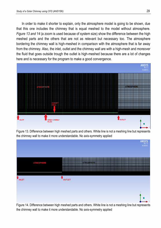
In order to make it shorter to explain, only the atmosphere model is going to be shown, due
that this one includes the chimney that is equal meshed to the model without atmosphere.
Figure 13 and 14 (a zoom is used because of system size) show the difference between the high
meshed parts and the others that are not as relevant but necessary too. The atmosphere
bordering the chimney wall is high-meshed in comparison with the atmosphere that is far away
from the chimney. Also, the inlet, outlet and the chimney wall are with a high-mesh and moreover
the fluid that goes outside trough the outlet is high-meshed because there are a lot of changes
here and is necessary for the program to make a good convergence.
Figure 13. Difference between high meshed parts and others. White line is not a meshing line but represents
the chimney wall to make it more understandable. No axis-symmetry applied
Figure 14. Difference between high meshed parts and others. White line is not a meshing line but represents
the chimney wall to make it more understandable. No axis-symmetry applied
30 Moya Chamizo Ricardo
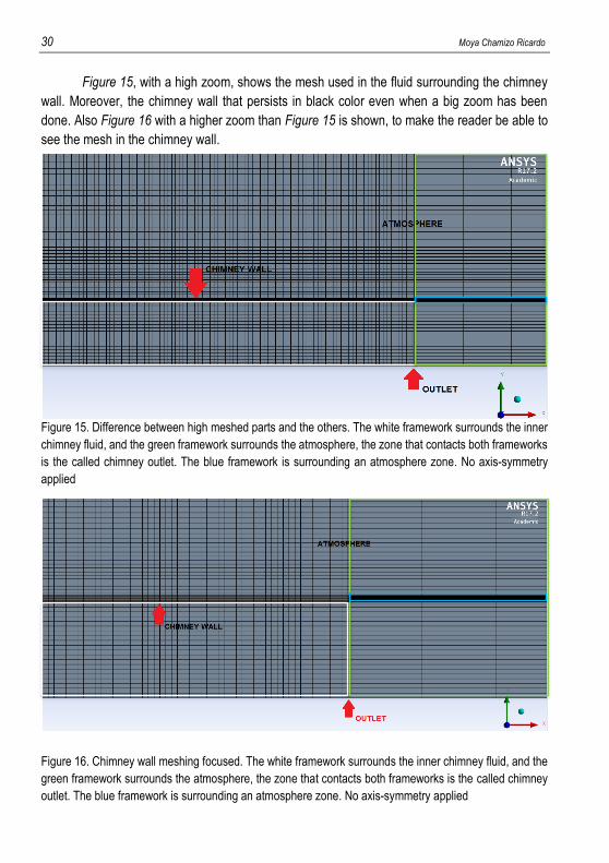
Figure 15, with a high zoom, shows the mesh used in the fluid surrounding the chimney
wall. Moreover, the chimney wall that persists in black color even when a big zoom has been
done. Also Figure 16 with a higher zoom than Figure 15 is shown, to make the reader be able to
see the mesh in the chimney wall.
Figure 15. Difference between high meshed parts and the others. The white framework surrounds the inner
chimney fluid, and the green framework surrounds the atmosphere, the zone that contacts both frameworks
is the called chimney outlet. The blue framework is surrounding an atmosphere zone. No axis-symmetry
applied
Figure 16. Chimney wall meshing focused. The white framework surrounds the inner chimney fluid, and the
green framework surrounds the atmosphere, the zone that contacts both frameworks is the called chimney
outlet. The blue framework is surrounding an atmosphere zone. No axis-symmetry applied

Study of a Solar Chimney using CFD (ANSYS®) 31
There is a need to say that a black meshing zone, persists in Figure 15 and 16. This zone
surrounded by the blue framework, represents a part of the atmosphere. This location is important
to be high meshed, because there will be high changes in the temperature, the density, the
velocity and the turbulence, due to the pure convection heat transfer outside the chimney.

32 Moya Chamizo Ricardo
5.3 Simulation setup
ANSYS® Fluent module is going to be used in this step. The two previous steps are general
for all ANSYS® simulation such as Static Structural, Transient Structural, Thermal-Electric, etc.
And once completed, the appropriate module is chosen to simulate the system behavior.
In this step the correct models, materials, boundary conditions, cell zone conditions, mesh
interfaces, reference values, etc. should be chosen. Is crucial to obtain a reliable solution. The
resolution methods and controls are established.
In the model definition section (multiphase, energy, viscous model, acoustics, etc.), where the
equations that will be used to calculate the process will be ready to check, one must consider the
mathematical model that governs the process to analyze. In Fluent case, there are several
mathematical models, the ones that are going to be used are the Turbulent k-∈ viscous model
and the energy model. There are composed of fluid flow equations, which are series of balances
and fluid properties, including the overall mass balance, known as the continuity equation, the
momentum balance, the energy balance, which is decomposed in different equations, and partial
mass balances. The information about the energy equations is extracted from (Krisst, 1983).
Those equations are:
Continuity
𝛿𝜌
𝛿𝑡+ 𝛻. (𝜌𝑈) = 𝑆𝑚 (1)
Momentum
𝛿𝜌𝑈
𝛿𝑡+ (𝛻. 𝜌𝑈𝑈) = −𝛻𝑝 + 𝛻. 𝜏 + 𝜌𝑔 (2)
𝜏 = µ [ (𝛻 𝑈 + 𝛻 𝑈𝑇) −2
3 𝛻 · 𝑈 𝐼] (3)
Enthalpy
𝛿𝜌𝐸
𝛿𝑡+ 𝛻. (𝑈(𝜌𝐸 + 𝜌)) = 𝛻. (𝑘𝑒𝑓𝑓 𝛻𝑇 − [∑ ℎ𝑗 𝐽𝑗 + (ẑ𝑒𝑓𝑓 · 𝑈)]𝑙 +Sh (4)
Study of a Solar Chimney using CFD (ANSYS®) 33
𝐸 = ℎ − 𝑃
𝜌+
𝑈2
2 (5)
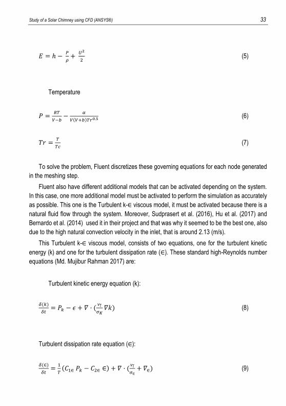
Temperature
𝑃 =𝑅𝑇
𝑉−𝑏−
𝛼
𝑉(𝑉+𝑏)𝑇𝑟0.5 (6)
𝑇𝑟 =𝑇
𝑇𝑐 (7)
To solve the problem, Fluent discretizes these governing equations for each node generated
in the meshing step.
Fluent also have different additional models that can be activated depending on the system.
In this case, one more additional model must be activated to perform the simulation as accurately
as possible. This one is the Turbulent k-∈ viscous model, it must be activated because there is a
natural fluid flow through the system. Moreover, Sudprasert et al. (2016), Hu et al. (2017) and
Bernardo et al. (2014) used it in their project and that was why it seemed to be the best one, also
due to the high natural convection velocity in the inlet, that is around 2.13 (m/s).
This Turbulent k-∈ viscous model, consists of two equations, one for the turbulent kinetic
energy (k) and one for the turbulent dissipation rate (∈). These standard high-Reynolds number
equations (Md. Mujibur Rahman 2017) are:
Turbulent kinetic energy equation (k):
𝛿(𝑘)
𝛿𝑡= 𝑃𝑘 − 𝜖 + 𝛻 · (
vT
𝜎𝐾𝛻𝑘) (8)
Turbulent dissipation rate equation (∈):
𝛿(∈)
𝛿𝑡=
1
𝑇(𝐶1∈ 𝑃𝑘 − 𝐶2∈ ∈) + 𝛻 · (
vT
𝜎∈+ 𝛻∈) (9)
34 Moya Chamizo Ricardo
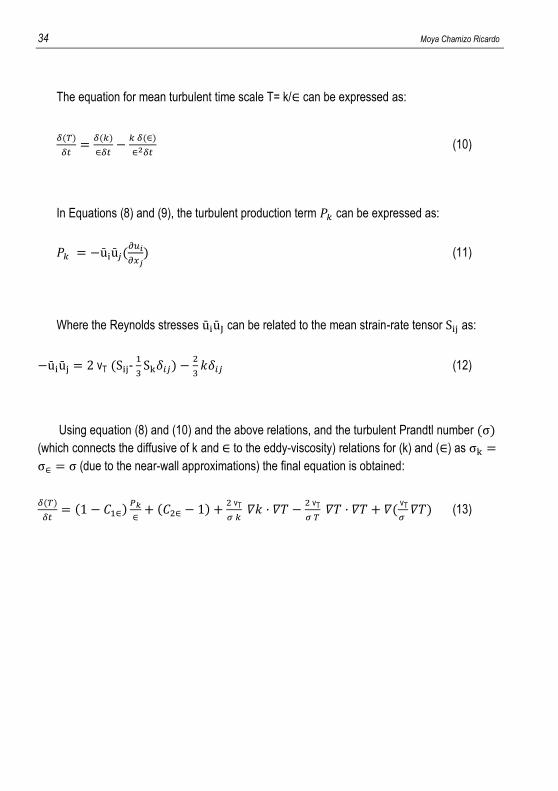
The equation for mean turbulent time scale T= k/∈ can be expressed as:
𝛿(𝑇)
𝛿𝑡=
𝛿(𝑘)
∈𝛿𝑡−
𝑘 𝛿(∈)
∈2𝛿𝑡 (10)
In Equations (8) and (9), the turbulent production term 𝑃𝑘 can be expressed as:
𝑃𝑘 = −ūiū𝑗(∂𝑢𝑖
∂𝑥𝑗) (11)
Where the Reynolds stresses ūiūJ can be related to the mean strain-rate tensor Sij as:
−ūiūj = 2 vT (Sij- 1
3Sk𝛿𝑖𝑗) −
2
3𝑘𝛿𝑖𝑗 (12)
Using equation (8) and (10) and the above relations, and the turbulent Prandtl number (σ)
(which connects the diffusive of k and ∈ to the eddy-viscosity) relations for (k) and (∈) as σk =
σ∈ = σ (due to the near-wall approximations) the final equation is obtained:
𝛿(𝑇)
𝛿𝑡= (1 − 𝐶1∈)
𝑃𝑘
∈+ (𝐶2∈ − 1) +
2 vT
𝜎 𝑘 𝛻𝑘 · 𝛻𝑇 −
2 vT
𝜎 𝑇 𝛻𝑇 · 𝛻𝑇 + 𝛻(
vT
𝜎 𝛻𝑇) (13)

Study of a Solar Chimney using CFD (ANSYS®) 35
Also, when the model and solver are checked, the most important part of the simulation (the
correct convergence of the calculations) must be checked too. Sometimes the project simulated
in ANSYS® Fluent have converge difficulties due to the residual errors or meshing and geometry
problems.
There are other kind of problems more difficult to correct. One of them is the non-convergence
between the equations and the nodes that have been created. To correct this, the URF
(under-relaxation factors) will be used. The pressure-based solver as this one, uses
under-relaxation of equations to control the update of computed variables at each iteration. This
means that all equations solved using the pressure-based solver, will have under-relaxation
factors associated with them.
In ANSYS® Fluent, the default under-relaxation parameters for all variables are set to values
that are near optimal for the largest possible number of cases. These values are suitable for many
problems, but for some particularly nonlinear problems (e.g., some turbulent flows or
natural-convection problems, as this one) it is prudent to reduce the under-relaxation factors
initially.
It is a good practice to begin a calculation using the default under-relaxation factors. If the
residuals continue to increase after the first 4 or 5 iterations, the best idea should be to reduce
the under-relaxation factors. Occasionally, it is important to make changes in the under-relaxation
factors and resume calculations, only to find that the residuals begin to increase. This often results
from increasing the under-relaxation factors too much.
The viscosity and density are under-relaxed from iteration to iteration (if they are variable as
in present work). Also, if the enthalpy equation is solved directly instead of the temperature
equation, the update of temperature based on enthalpy will be under-relaxed.
For most flows, the default under-relaxation factors do not usually require modification. If
unstable or divergent behavior is observed, however, a great reduction of the under-relaxation
factors for pressure, momentum, k, and ∈ from their default values to about 0.2, 0.5, 0.5 and 0.5,
respectively, would be fine if the simulation is like this one. In problems where density is strongly
coupled with temperature, as in very high Rayleigh number natural convection as this project or
in mixed convection flows, it is wise to also under-relax the temperature equation and/or density.
For other scalar equations (e.g., swirl, species, mixture fraction and variance) the default
under-relaxation factors may be too aggressive for some problems, especially at the beginning of
the calculation. Those should be reduced to 0.8 to facilitate convergence.
36 Moya Chamizo Ricardo
6. RESULTS AND DISCUSSION
As described before, the most important variables to analyze in a solar chimney with natural
convection are temperature, density and velocity in each point of the system. Therefore, their
profiles, contours and distributions will be discussed.
Furthermore, another important values and longitudinal image distributions will be exposed in
order to understand better the simulation, as for example, the surface heat transfer coefficients
for the chimney walls in contact with indoor and outdoor air. Also, the turbulent distributions are
shown inside and outside the chimney, and the Reynolds values in each height.
Moreover, there is a need to say that the graphics will be exported from ANSYS® Fluent
setup, because there are so much nodes, and it is impossible to transfer all the data in to Excel
or any other program that allows to build graphics.
The distribution contour pictures, the graphics and the non-graphical results that are going to
be shown will be exposed in the following order:
- Temperature contours, graphics and integrals
- Density contours, graphics and integrals
- Velocity contours, graphics and integrals
Study of a Solar Chimney using CFD (ANSYS®) 37
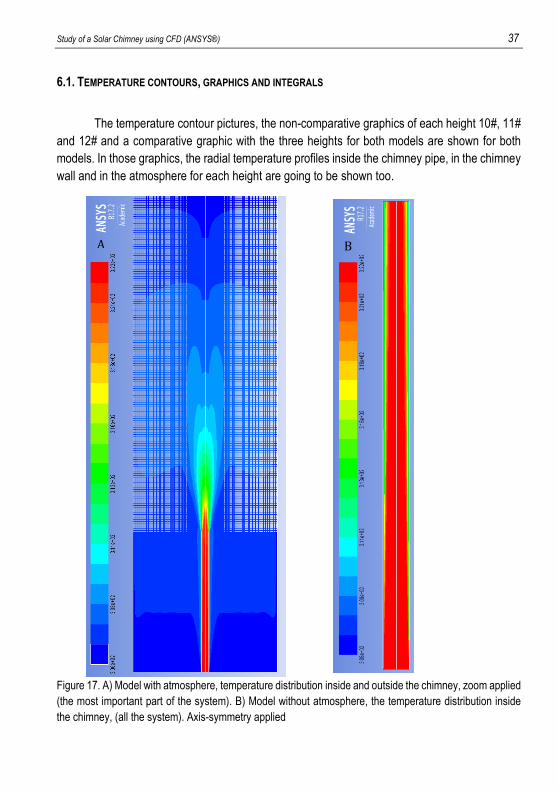
6.1. TEMPERATURE CONTOURS, GRAPHICS AND INTEGRALS
The temperature contour pictures, the non-comparative graphics of each height 10#, 11#
and 12# and a comparative graphic with the three heights for both models are shown for both
models. In those graphics, the radial temperature profiles inside the chimney pipe, in the chimney
wall and in the atmosphere for each height are going to be shown too.
Figure 17. A) Model with atmosphere, temperature distribution inside and outside the chimney, zoom applied
(the most important part of the system). B) Model without atmosphere, the temperature distribution inside
the chimney, (all the system). Axis-symmetry applied
A)
B)

38 Moya Chamizo Ricardo
Figure 18. A) Model with atmosphere, 10#, 10# chim and 10# atm radial temperature profiles inside and
outside the chimney. The vertical black line references the chimney wall. B) Model without atmosphere,
radial temperature profile of 10#. (These are not comparative graphics)
Figure 19. A) Model with atmosphere, 11#, 11# chim and 11# atm radial temperature profiles inside and
outside the chimney. The vertical black line references the chimney wall. B) Model without atmosphere,
radial temperature profile of 11#. (These are not comparative graphics)
Figure 20. A) Model with atmosphere, 12#, 12# chim and 12# atm radial temperature profiles inside and
outside the chimney. The vertical black line references the chimney wall. B) Model without atmosphere,
radial temperature profile of 12#. (These are not comparative graphics)
A)
B)
B)
B)
A)
A)
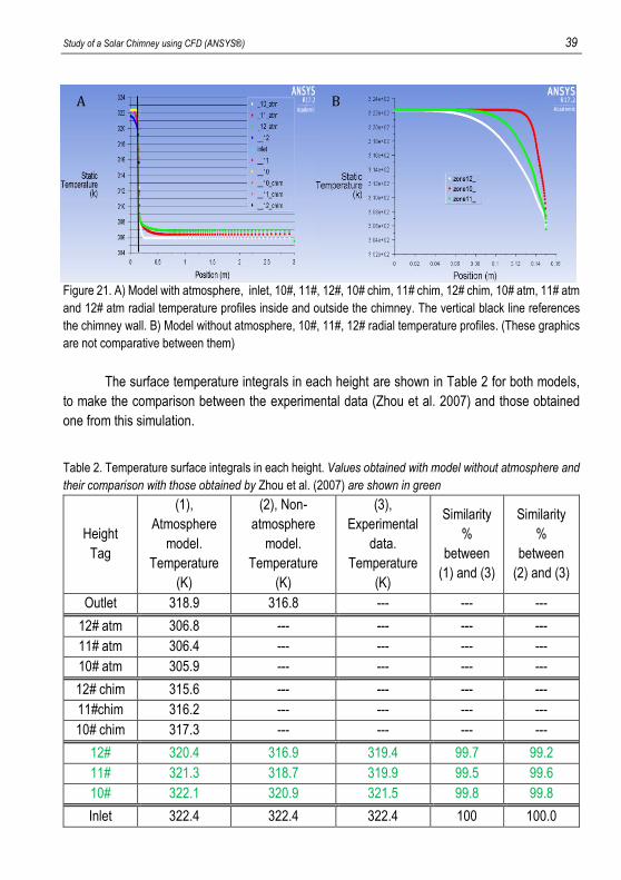
Study of a Solar Chimney using CFD (ANSYS®) 39
Figure 21. A) Model with atmosphere, inlet, 10#, 11#, 12#, 10# chim, 11# chim, 12# chim, 10# atm, 11# atm
and 12# atm radial temperature profiles inside and outside the chimney. The vertical black line references
the chimney wall. B) Model without atmosphere, 10#, 11#, 12# radial temperature profiles. (These graphics
are not comparative between them)
The surface temperature integrals in each height are shown in Table 2 for both models,
to make the comparison between the experimental data (Zhou et al. 2007) and those obtained
one from this simulation.
Table 2. Temperature surface integrals in each height. Values obtained with model without atmosphere and
their comparison with those obtained by Zhou et al. (2007) are shown in green
Height
Tag
(1),
Atmosphere
model.
Temperature
(K)
(2), Non-
atmosphere
model.
Temperature
(K)
(3),
Experimental
data.
Temperature
(K)
Similarity
%
between
(1) and (3)
Similarity
%
between
(2) and (3)
Outlet 318.9 316.8 --- --- ---
12# atm 306.8 --- --- --- ---
11# atm 306.4 --- --- --- ---
10# atm 305.9 --- --- --- ---
12# chim 315.6 --- --- --- ---
11#chim 316.2 --- --- --- ---
10# chim 317.3 --- --- --- ---
12# 320.4 316.9 319.4 99.7 99.2
11# 321.3 318.7 319.9 99.5 99.6
10# 322.1 320.9 321.5 99.8 99.8
Inlet 322.4 322.4 322.4 100 100.0
B)
A)

40 Moya Chamizo Ricardo
The longitudinal surface heat transfer coefficients values that have been obtained from
the external chimney wall layer in contact with the atmosphere layer, and from the interior chimney
wall layer in contact with the interior fluid layer, are going to be shown in a table 3.
Table 3. Surface heat transfer coefficients that have been obtained from a longitudinal integral in the
corresponding layers
Tag
Atmosphere model.
Surface heat transfer
coefficient [W/(m2·K)]
Non-atmosphere model.
Surface heat transfer
coefficient [W/(m2·K)]
Atmosphere – chimney wall 1.30 ---
Interior fluid – chimney wall 1.40 6.84
In Figure 17 where the temperature distribution is shown, it is important to consider the
chimney inlet. The inlet temperature is 322.4 K for both models, with this temperature at the
beginning of the simulation, the contours complete the energy equations showing the temperature
distributions. The heat flow goes to the pipe wall by convection heat transfer through the fluid and
through the pipe wall by conduction heat transfer. Only in the atmosphere model it goes with
convection heat transfer trough the atmosphere.
In the atmosphere model, the temperature is smaller in the upper parts of the chimney,
because the wall absorbs heat and it leaks to the surrounding atmosphere. The same happens in
the non-atmosphere model but the heat goes nowhere in the simulation because there is no layer
there.
In the same Figure 17 and focusing on the atmosphere model, near the chimney outlet,
in the outdoors, a “tongue” can be seen, this one is created because there is only convection heat
transfer due that there is not a wall. This causes a faster heat exchange and the temperature of
the air increases faster. But the temperature goes down to the atmosphere one 305.5 K at
approximately 30 m tall.
In Figures 18, 19, 20 and 21 the radial temperature profiles can be seen for both models.
Focusing in Figure 21, the B) that corresponds to the non-atmosphere model, only shows the
temperature inside the pipe at different heights. It has the same behavior as the atmosphere
model, A). In A) case, the temperature in 10# (_10) is higher that the temperature in 11# (_11)
and 12# (_12), because in the inlet the temperature is 322.4 K and the heat is liberated from the
pipe to the atmosphere reducing the temperature inside the chimney. The same happens in the
wall, in 10# chim (_10_chim) the temperature is higher than in 11# chim (_11_chim) and in 12#
chim (_12_chim). But something different happens outside the chimney, were the temperature
before running the simulation is 305.5 K. The temperature in 12# atm (_12_atm) is higher than in

Study of a Solar Chimney using CFD (ANSYS®) 41
11# atm (_11_atm) and this one is higher than the temperature in 10# atm (_10_atm). This
happens because the temperature in the atmosphere grows up when the chimney inner
temperature goes down due to the heat flow released to the outside.
In table 2, it is important to see that the temperature is not the same, but it is close for
both models. In the atmosphere model, the simulation was carried without air convection in the
atmosphere. This means that in the simulation it was a static fluid before the temperature started
changing its density and the natural advection started. This convection would directly take part in
the temperature of the wall, cooling it and reducing the inner chimney temperature to the wanted
one. In order to check this, the values of the non-atmosphere model, which has a constant
temperature boundary condition at the chimney wall, are shown in table 2.
In the atmosphere model, the heat transfer coefficients that can be seen in table 3 are
very low values. This is caused because the air started the simulation as static fluid, and all the
convection that was created in the simulation was due to the natural advection of the fluid.
In the non-atmosphere model, the heat transfer coefficient at the outdoor is supposed to
be very high because of the constant temperature boundary condition, (cannot obtain the value
because there is not a layer there to obtain it). Due to this, the indoor heat transfer coefficient in
the non-atmosphere model is higher than in the atmosphere model.
In this case an additional Figure 22 is build, to make the reader have an idea about the
temperature fluctuations in the longitudinal axis inside the chimney wall for the atmosphere model.
Figure 22. Temperature profile inside the chimney wall in the longitudinal axis (h = height) (interior-solid =
interior wall, which means the interior part of the chimney wall)
h

42 Moya Chamizo Ricardo
The Figure 22 corresponds to the atmosphere model. There is no chance to obtain a
graphic like this one for the non-atmosphere model, because the boundary condition in the
chimney wall, is a constant temperature. This boundary condition simulates a high convection. In
order to make the reader understand better the difference between the 2 models, a new two
graphics (Figure 23) with the temperature profiles of 10#, 11# and 12# heights inside the chimney
pipe are going to be shown.
Figure 23. A) Model with atmosphere, 10#, 11# and 12# radial temperature profiles inside the chimney. B)
Model without atmosphere, 10#, 11#, 12# radial temperature profiles. (These graphics are comparative
between them)
B)
A)

Study of a Solar Chimney using CFD (ANSYS®) 43
6.2. DENSITY CONTOURS, GRAPHICS AND INTEGRALS
The density contour pictures, the graphics of each height 10#, 11# and 12#, a comparative
graphic with the three heights and a table will show in this section for both models. In those
graphics, the radial density profiles inside the chimney pipe and in the atmosphere for each height
will also show.
Figure 24. A) Model with atmosphere, density distribution inside and outside the chimney, zoom applied (the
most important part of the system). B) Model without atmosphere, density distribution inside the chimney,
(all the system). Axis-symmetry applied
A)
B)
44 Moya Chamizo Ricardo
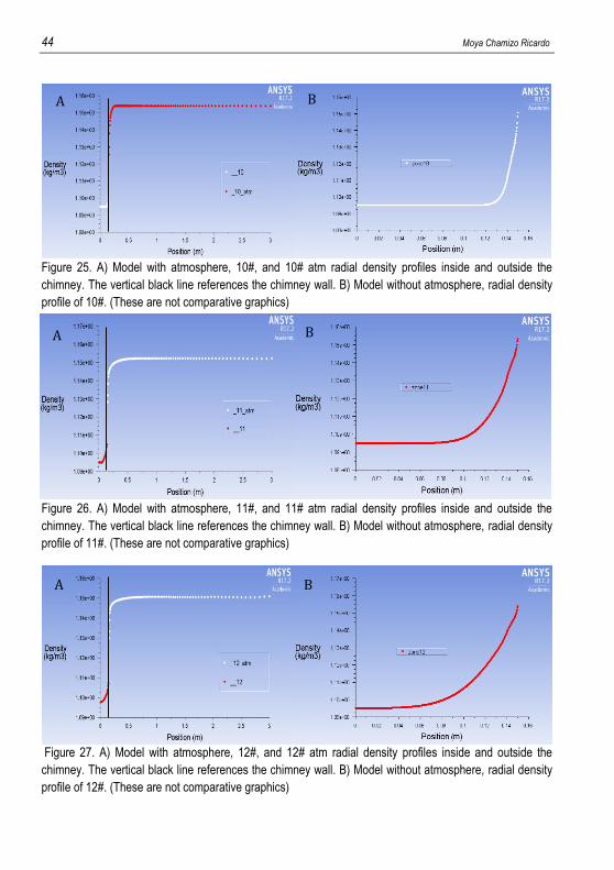
Figure 25. A) Model with atmosphere, 10#, and 10# atm radial density profiles inside and outside the
chimney. The vertical black line references the chimney wall. B) Model without atmosphere, radial density
profile of 10#. (These are not comparative graphics)
Figure 26. A) Model with atmosphere, 11#, and 11# atm radial density profiles inside and outside the
chimney. The vertical black line references the chimney wall. B) Model without atmosphere, radial density
profile of 11#. (These are not comparative graphics)
Figure 27. A) Model with atmosphere, 12#, and 12# atm radial density profiles inside and outside the
chimney. The vertical black line references the chimney wall. B) Model without atmosphere, radial density
profile of 12#. (These are not comparative graphics)
A)
A)
A)
B)
B)
B)

Study of a Solar Chimney using CFD (ANSYS®) 45
Figure 28. A) Model with atmosphere, inlet, 10#, 11#, 12#,10# atm, 11# atm and 12# atm radial density
profiles inside and outside the chimney. The vertical black line references the chimney wall. B) Model without
atmosphere, 10#, 11#, 12# radial density profiles. (These graphics are not comparative between them)
Table 4: Density surface integrals in each height. In this case, there is no comparison between the
experimental data (Zhouet al. 2007) and the simulation data, because experimental density is unknown
Height Tag
(1), Atmosphere
model.
Density (kg/m3)
(2), Non-
atmosphere model.
Density (kg/m3)
Similarity % between
(1) and (2)
Outlet 1.106 1.116 99.10
12# atm 1.151 --- ---
11# atm 1.152 --- ---
10# atm 1.154 --- ---
12# 1.105 1.114 99.19
11# 1.102 1.107 99.54
10# 1.097 1.100 99.72
Inlet 1.095 1.095 100.00
Figure 24 shows the density distribution for both models. The picture is like the
temperature one, but with reversed colors. This effect is caused due that the density is a
temperature function. When the temperature changes, the density inversely changes.
The density is the cause of the fluid buoyancy. It is the induction force that will make the
fluid to move up through the chimney. It is important to say that the weather depends directly on
the results. The atmosphere temperature is around 305.5 K in the atmosphere model, and in the
non-atmosphere model the chimney wall is always at 305.5 K. This means that the difference
between the density inside the chimney pipe and outside it, is not as different as it could be in
winter temperatures. Moreover, in the atmosphere model, the heat flow that goes outside the
chimney, is the one that makes the interior chimney fluid to be colder near the walls than in the
A)
B)

46 Moya Chamizo Ricardo
center of the pipe. Due to this, the density in this chimney part is higher than in the middle of it,
where the temperature is maintained and the density is nearly to be constant. The same happens
in the non-atmosphere model, the program knows that the heat flow must go out, but it cannot be
seen due there is no layer there.
This higher density near the chimney wall, which can be seen in both models, is such an
important characteristic of the system. The fluid doesn’t go up at the same velocity in those parts.
That lower velocity near the walls makes the fluid to become a wall in comparison with the fluid
that is in the middle of the pipe. Due to this, the effective diameter where the fluid is circulating
through is being reduced. This diameter reduction caused by the high-density fluid near the walls
is such a section reduction. Therefore, this effect is creating a velocity increment in the middle
part of the chimney where the fluid will go faster.
In the atmosphere model, concretely in the outlet of the chimney, a “tongue” can be seen,
this is created because there is only convection heat transfer due that there is not a wall. This
means that, the heat exchange is faster through the atmosphere and the temperature increases
faster reducing the density in each point. The temperature goes down to the atmosphere one
305.5 K at approximately 30 m tall, which means that the density will be higher there.
Figures 25, 26, 27 and 28 show the radial density profiles for both models. Focusing on
Figure 28, the case B), that corresponds to the non-atmosphere model, shows the density inside
the pipe at different heights. In B) case, the density has the same behavior as in the atmosphere
model A) inside the pipe. The density in 12# (_12) is higher that the density in 11# (_11) and 10#
(_10), because in the inlet the temperature is 322.4 K and the heat is liberated from the pipe
reducing the temperature inside the chimney and thereby increasing the density near the walls.
In the atmosphere model, something different happens outside the chimney, where the
temperature before running the simulation was 305.5 K. The density in 10# atm (_10_atm) is
higher than in 11# atm (_11_atm) and this one is higher than the density in 12# atm (_12_atm),
this happens because the air temperature increases when the chimney inner temperature
decreases due to the heat flux that is liberated to the atmosphere. This effect will decrease the
density in the higher parts of the chimney. In the A) case, concretely in the atmosphere, a constant
density zone can be seen, because the heat flux is not too high to change the temperature of the
fluid that is far away from the chimney wall. This happens in all the heights where there is a
chimney wall domain. When the chimney pipe finishes the above mentioned “tongue”, changes
the temperature of that atmosphere easily, due that there is not a wall. Therefore, the density is
changing there too.
In table 4, it is important to note that there is no comparison between the experimental
data (Zhou et al. 2007) and present simulation data.
When a simulation is performed, all the results as temperature, density and velocity will
be obtained at once. If the temperature values are correct, the density values will be correct too.

Study of a Solar Chimney using CFD (ANSYS®) 47
6.3. VELOCITY CONTOURS, GRAPHICS AND INTEGRALS
The velocity contour pictures and the graphics of each height 10#, 11# and 12# and a
comparative graphic with the three heights will be shown in the present section for both models.
In those graphics, the radial velocity profiles inside the chimney pipe and in the atmosphere for
each height will be shown too.
Figure 29. A) Model with atmosphere, velocity distribution inside and outside the chimney, zoom applied (the
most important part of the system). B) Model without atmosphere, velocity distribution inside the chimney,
(all the system). Axis-symmetry applied
A)
B)

48 Moya Chamizo Ricardo
Figure 30. A) Model with atmosphere, 10#, and 10# atm radial velocity profiles inside and outside the
chimney. The vertical black line references the chimney wall. B) Model without atmosphere, radial velocity
profile of 10#. (These are not comparative graphics)
Figure 31. A) Model with atmosphere, 11#, and 11# atm radial velocity profiles inside and outside the
chimney, the vertical black line references the chimney wall. B) Model without atmosphere, radial velocity
profile of 11#. (These are not comparative graphics
Figure 32. A) Model with atmosphere, 12#, and 12# atm radial velocity profiles inside and outside the
chimney. The vertical black line references the chimney wall. B) Model without atmosphere, radial velocity
profile of 12#. (These are not comparative graphics)
A)
A)
A)
B)
B)
B)

Study of a Solar Chimney using CFD (ANSYS®) 49
Figure 33. A) Model with atmosphere, inlet, 10#, 11#, 12#,10# atm, 11# atm and 12# atm radial velocity
profiles inside and outside the chimney. The vertical black line references the chimney wall. B) Model without
atmosphere, 10#, 11#, 12# radial velocity profiles. (These graphics are not comparative between them)
The surface velocity integrals of each height are shown in table 5 and the surface Reynolds
integrals of each height will be shown in table 6, to show the flux model.
Table 5: Velocity surface integrals in each height. In this case, there is no comparison between the
experimental data (Zhou et al. 2007) and the simulation data, because velocity experimental data is unknown
Height Tag
(1), Atmosphere
model.
Velocity (m/s)
(2), Non-atmosphere
model. Velocity (m/s)
Similarity %
between (1) and
(2)
Outlet 2.111 2.094 99.19
12# atm 0.030 --- ---
11# atm 0.014 --- ---
10# atm 0.003 --- ---
12# 2.118 2.095 99.71
11# 2.124 2.107 99.71
10# 2.128 2.122 99.99
Inlet 2.130 2.130 100
A)
B)

50 Moya Chamizo Ricardo
Table 6: Reynolds surface integrals for both models at each height. There is no comparison between the
experimental data (Zhou et al. 2007) and the simulation data, because Reynolds experimental data is
unknown
Height Tag (1), Atmosphere model.
Reynolds
(2), Non-atmosphere
model.
Reynolds
Similarity %
between (1)
and (2)
Outlet 18.211 17.957 98.61
12# atm 1.132 --- ---
11# atm 3.127 --- ---
10# atm 2.352 --- ---
12# 18.876 17.971 95.21
11# 44.648 18.165 40.68
10# 94.459 18.348 19.42
Inlet 84.798 20.316 23.95

Study of a Solar Chimney using CFD (ANSYS®) 51
In this case, some additional pictures are built to show the behavior of velocity contours
and vectors near the walls in both models. To show this effect, some pictures with a high zoom
and vertical format are used. Also, a picture for the air turbulence was built for both models.
Figure 34. A) Model with atmosphere, velocity contour, zoom applied. Left picture, fluid entrance into the
system. Right picture, continuation of the left picture until the outlet. Axis-symmetry applied
A)
A)

52 Moya Chamizo Ricardo
Figure 35. A) Model with atmosphere, velocity vectors, zoom applied. Left picture, fluid entrance into the
system. Right picture, continuation of the left picture until the outlet. Axis-symmetry applied
A)
A)

Study of a Solar Chimney using CFD (ANSYS®) 53
Figure 36. B) Model without atmosphere, velocity vectors, zoom applied. Left picture, fluid entrance into the
system. Right picture, continuation of the left picture until the outlet. No axis-symmetric applied, only radial
direction
B)
B)

54 Moya Chamizo Ricardo
Figure 37. A) Model with atmosphere, turbulence distribution inside and outside the chimney, zoom applied (the most important part of the system). B) Model without atmosphere, turbulence distribution inside the chimney, (all the system). Axis-symmetry applied
A)
B)
Study of a Solar Chimney using CFD (ANSYS®) 55
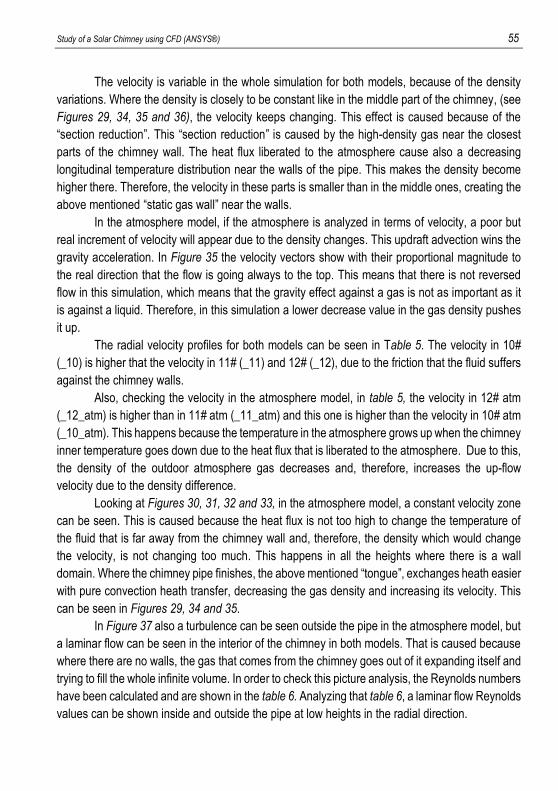
The velocity is variable in the whole simulation for both models, because of the density
variations. Where the density is closely to be constant like in the middle part of the chimney, (see
Figures 29, 34, 35 and 36), the velocity keeps changing. This effect is caused because of the
“section reduction”. This “section reduction” is caused by the high-density gas near the closest
parts of the chimney wall. The heat flux liberated to the atmosphere cause also a decreasing
longitudinal temperature distribution near the walls of the pipe. This makes the density become
higher there. Therefore, the velocity in these parts is smaller than in the middle ones, creating the
above mentioned “static gas wall” near the walls.
In the atmosphere model, if the atmosphere is analyzed in terms of velocity, a poor but
real increment of velocity will appear due to the density changes. This updraft advection wins the
gravity acceleration. In Figure 35 the velocity vectors show with their proportional magnitude to
the real direction that the flow is going always to the top. This means that there is not reversed
flow in this simulation, which means that the gravity effect against a gas is not as important as it
is against a liquid. Therefore, in this simulation a lower decrease value in the gas density pushes
it up.
The radial velocity profiles for both models can be seen in Table 5. The velocity in 10#
(_10) is higher that the velocity in 11# (_11) and 12# (_12), due to the friction that the fluid suffers
against the chimney walls.
Also, checking the velocity in the atmosphere model, in table 5, the velocity in 12# atm
(_12_atm) is higher than in 11# atm (_11_atm) and this one is higher than the velocity in 10# atm
(_10_atm). This happens because the temperature in the atmosphere grows up when the chimney
inner temperature goes down due to the heat flux that is liberated to the atmosphere. Due to this,
the density of the outdoor atmosphere gas decreases and, therefore, increases the up-flow
velocity due to the density difference.
Looking at Figures 30, 31, 32 and 33, in the atmosphere model, a constant velocity zone
can be seen. This is caused because the heat flux is not too high to change the temperature of
the fluid that is far away from the chimney wall and, therefore, the density which would change
the velocity, is not changing too much. This happens in all the heights where there is a wall
domain. Where the chimney pipe finishes, the above mentioned “tongue”, exchanges heath easier
with pure convection heath transfer, decreasing the gas density and increasing its velocity. This
can be seen in Figures 29, 34 and 35.
In Figure 37 also a turbulence can be seen outside the pipe in the atmosphere model, but
a laminar flow can be seen in the interior of the chimney in both models. That is caused because
where there are no walls, the gas that comes from the chimney goes out of it expanding itself and
trying to fill the whole infinite volume. In order to check this picture analysis, the Reynolds numbers
have been calculated and are shown in the table 6. Analyzing that table 6, a laminar flow Reynolds
values can be shown inside and outside the pipe at low heights in the radial direction.

56 Moya Chamizo Ricardo
7. CONCLUSIONS
1- After studying the state of the art of solar chimney simulations it can be stated that this work
presents the first simulation of solar chimney with surrounding atmosphere. The atmosphere
model of this project is determined as representative, given the similarity between the
obtained results and the experimental data (Zhou, et al. 2007). Emphasizing the temperature
results obtained in the simulation, in the different predetermined heights, it is concluded that
the similarity between these and the experimental data is 99.7%.
2- After studying the state of the art of solar chimney simulations in ANSYS® Fluent, and
knowing that it is the model used by other authors. The non-atmosphere model of this project
is determined as representative, given the similarity between the results obtained and the
experimental data (Zhou, et al. 2007). Emphasizing the temperature results obtained in the
simulation, in the different predetermined heights, it is concluded that the similarity between
these and the experimental data is 99.5%.
3- Considering that the goal of the study is to compare the results with the existing real data
and not to design a device, both models are equally valid, but the atmosphere model is more
representative.
4- Validated the temperature results for both models, it is possible to say that the obtained
results of density, velocity and turbulence are expected to match with the experimental data
(Zhou, et al. 2007).
5- Thanks to the atmosphere model, it has been possible to confirm changes of speed in the
air surrounding the chimney given the variation in its density. By overcoming the action of
gravity, all the surrounding air generates upward currents.
Study of a Solar Chimney using CFD (ANSYS®) 57
8. RECOMMENDATIONS
The following recommendations are based on trial and error tests. Also of knowledge
obtained throughout the simulation process. And, obtained from other sources of information related to ANSYS Fluent, such as the Workbench operator's manual and the ANSYS® Fluent users guide.
- The use of "URF" relaxation factors is recommended whenever possible (see page 35).
- It is recommended to always carry out 2D solar chimney studies whenever possible,
using the symmetry of the systems, to avoid unnecessary node calculation. Especially, in cases where other systems are adapted to the chimney or if it is a case with atmosphere, because of the substantial number of nodes generated.
- It is recommended the square meshing, to facilitate the computation of the results.
- To design a solar chimney it is recommended to do it with a model that includes an
atmosphere. With an atmosphere surrounding the pipe, the outdoor possible impacts can be known.
- If it is desired to design a solar chimney in conjunction with a structure, be it a building or an installation, it is recommended to use the model with atmosphere if many nodes are available. In case that enough nodes are not available it is recommended to make the model without atmosphere, since the approximation will be correct enough.
- If it is desired to evaluate the interior behavior of the chimney, against external variations,
whether changes of humidity, air velocity, ambient temperature, solar radiation, changes in the composition of the outside air, chimney construction materials, etc. It is recommended to use a model with atmosphere.
- If it is desired to evaluate the interior behavior of the chimney, against changes in
temperature, pressure, speed, composition, etc. It is recommended to use any model. The approximations that will give both will be very similar.
58 Moya Chamizo Ricardo
9. FUTURE WORK
The project can be extended by different means, among others:
1- Addition:
a. Of a structure under the chimney, being it a collector, a building, a factory, or
a house, attaching to them an entrance of air.
b. Once a system such as case (a) has been added, an air humidification system
at the entrance can be added to it to reduce the temperature of the area and
thus to create a more adequate ventilation system. Also, a good idea would
be adding a cooling system in the air intake without having to change the
composition of it.
c. Add a turbine to the chimney top to take advantage of the kinetic energy of
the fluid and create electrical energy.
2- Behavioral evaluation of the chimney:
a. Against changes in solar radiation, whether changes in the angle or intensity
of incident radiation.
b. If there are modifications in the building materials of the chimney.
c. If the fluid were flue gases, instead of natural air.
d. Changing the indoor flow composition.
e. Changing the outdoor fluid composition.
f. Changing the outdoor temperature and humidity.
These ideas are proposed to carry out a much more exhaustive and concrete study of this phenomenon, being able to contribute in the creation of a new concept of ventilation for living homes or industries, applicable anywhere in the world and being completely free, sustainable and natural.

Study of a Solar Chimney using CFD (ANSYS®) 59
10. REFERENCES AND NOTES
Bernardo Buonomo et al. Thermal and fluid dynamic analysis of solar chimney building
systems.Via Roma 29, 81031 Aversa (CE), Italy,ResearchGate,2014.
Hu Siyang, Dennis Y.C.Leung, Jhon C.Y.Chan Impact of the geometry of divergent chimneys
on the power output of a solar chimney power plant.Pokfulan Road, Hong Kong, China /
Shilong South Road, Foshan, Guangdong 528200, China,ELSEVIER,2017.
Islamuddin Azeemuddin, HussainH Al-Kayiem and Syed I Gilani Simulation of solar
chimney power plant with an external heat source.Department of Mechanical Engineering,
Universiti of Teknologi Petronas, Malaysia,IOPSCIENCE,2013.
Krisst R.J.K Energy transfer system. Energy 63, 8-11.Alt. Sour.,s.n.,1983.
Kulunk A prototype solar convection chimney operated under Izmit conditions.Miami Beach,
Florida,Proceddings of 7th Miami International Conference on Alternative Energy Sources
Md. Mujibur Rahman Ville Vuorinen, Ramesh K. Agarwal, Md Mizanur Rahman One-
Equation Turbulence Model Based on k/epsilon.s.l.,Conference SciTech,2017.
N. Pasumarthi S.A.Sherif Experimental and theoretical performance of a demonstration solar
chimney model.s.l.,International Journal of Energy Research,1998.
Sudprasert Sudaporn, Chatchawin Chinsorranant, Phadungsak Rattanadecho Numerical
study of vertical solar chimneys with moist air in a hot and humid climate.Klontuang,
Patumthani, Thailand,ELSEVIER,2016.
Zhou Xinping et al. Experimental study of temperature field in a solar chimney power setup.1037 Luoyu Road. Wuhan, Hubei 430074, China,ELSEVIER,2007.
ANSYS Fluent User's Guide, ANSYS®s.l.,ANSYS, inc. Southpointe 275 Technology Drive
Canonsburg, PA 15317.
60 Moya Chamizo Ricardo
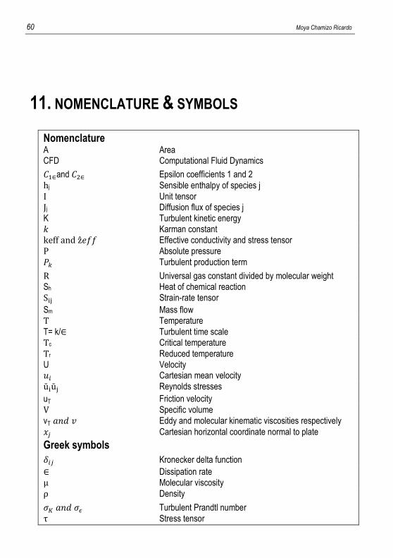
11. NOMENCLATURE & SYMBOLS
Nomenclature A Area CFD Computational Fluid Dynamics
𝐶1∈and 𝐶2∈ Epsilon coefficients 1 and 2
hj Sensible enthalpy of species j
I Unit tensor Jj Diffusion flux of species j K Turbulent kinetic energy 𝑘 Karman constant keff and ẑ𝑒𝑓𝑓 Effective conductivity and stress tensor
P Absolute pressure
𝑃𝑘 Turbulent production term
R Universal gas constant divided by molecular weight Sh Heat of chemical reaction Sij Strain-rate tensor
Sm Mass flow T Temperature
T= k/∈ Turbulent time scale Tc Critical temperature
Tr Reduced temperature U Velocity 𝑢𝑖 Cartesian mean velocity
ūiūj Reynolds stresses
uT Friction velocity
V Specific volume vT 𝑎𝑛𝑑 𝑣 Eddy and molecular kinematic viscosities respectively
𝑥𝑗 Cartesian horizontal coordinate normal to plate
Greek symbols
𝛿𝑖𝑗 Kronecker delta function
∈ Dissipation rate µ Molecular viscosity
ρ Density
𝜎𝐾 𝑎𝑛𝑑 𝜎𝜖 Turbulent Prandtl number
τ Stress tensor

Study of a Solar Chimney using CFD (ANSYS®) 61
62 Moya Chamizo Ricardo
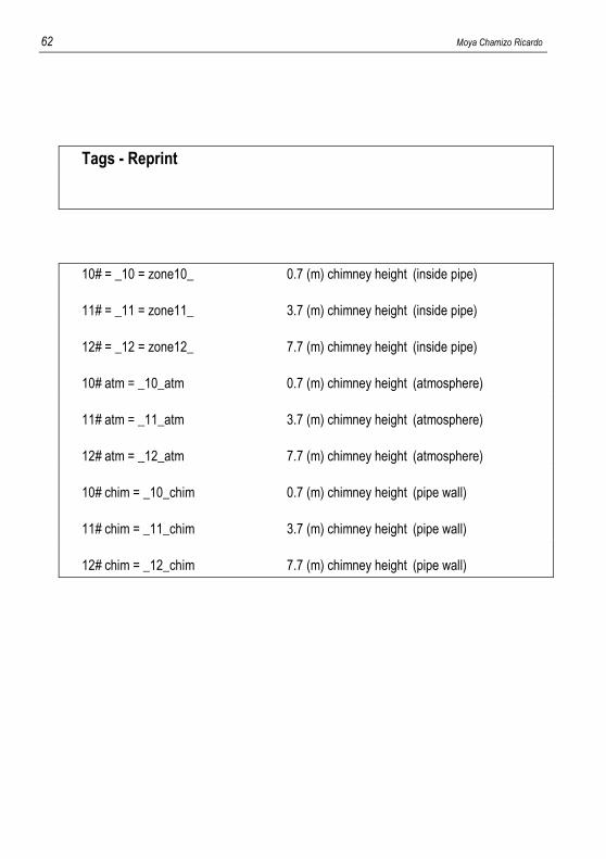
Tags - Reprint
10# = _10 = zone10_ 0.7 (m) chimney height (inside pipe)
11# = _11 = zone11_ 3.7 (m) chimney height (inside pipe)
12# = _12 = zone12_ 7.7 (m) chimney height (inside pipe)
10# atm = _10_atm 0.7 (m) chimney height (atmosphere)
11# atm = _11_atm 3.7 (m) chimney height (atmosphere)
12# atm = _12_atm 7.7 (m) chimney height (atmosphere)
10# chim = _10_chim 0.7 (m) chimney height (pipe wall)
11# chim = _11_chim 3.7 (m) chimney height (pipe wall)
12# chim = _12_chim 7.7 (m) chimney height (pipe wall)