Embed Size (px)
Citation preview
Treball Final de Grau
Tutor/s
Dr. David Curcó Cantarell Departament d’Enginyeria Química
Obtaining distillation and residue curves for nonideal ternary systems.
Obtención de curvas de destilación y residuo para sistemas ternarios no ideales.
Héctor Cruzado Valverde January 2015


Aquesta obra esta subjecta a la llicència de: Reconeixement–NoComercial-SenseObraDerivada
http://creativecommons.org/licenses/by-nc-nd/3.0/es/

No podemos resolver problemas pensando de la misma manera que cuando los creamos.
Albert Einstein
Agradecimientos a las personas que me han acompañado en este viaje que ha sido la
universidad: mis padres, compañeros, amigos, tutores y profesores. Sin duda alguna ese apoyo
recibido me ha influenciado y ayudado a alcanzar mis metas.
Agradezco el esfuerzo que han puesto mis padres al invertir en mi educación.
Este trabajo no podría haberse completado sin la gran ayuda que ha sido mi tutor de TFG, el
Dr. David Curcó, parte de su trabajo se encuentra en el programa creado.
La universidad ha sido para mí una experiencia placentera y me ha hecho progresar de
muchas maneras, el camino puede ser difícil a veces pero con dedicación podemos resolver
cualquier problema y al hacerlo sabemos que hemos aprendido algo nuevo. Aún queda un largo
camino, y aún más por aprender.


REPORT

Obtaining distillation and residue curves for nonideal ternary systems 1
CONTENTS
1. SUMMARY 3
2. RESUM 5
3. INTRODUCTION 7
3.1. 1st Residue curve map 8
3.1.1. 2nd Residue curves 9
3.1.2. 2nd Thermodynamic model and considerations 10
3.1.2.1. 3rd UNIFAC model 10
3.1.2.2. 3rd Ideal vapour phase 11
3.1.2.3. 3rd Liquid-Vapour equilibrium 11
3.1.2.4. 3rd Vapour pressure 12
3.1.3. 2nd Features of RCM 12
3.2. 1st Distillation curve map 13
3.2.1. 2nd Distillation curves 15
3.2.2. 2nd Thermodynamic model and considerations 16
3.2.3. 2nd Distillation borders 16
4. OBJECTIVES 16
5. DEVELOPMENT: RCM DESIGNER 17
5.1. 1st Bibliography review 17
5.2. 1st Election of the algorithm 17
5.3. 1st Codification 18
5.4. 1st Validation of the results 19
6. RESULTS AND DISCUSSION 20
6.1. 1st Sections of the program 20
6.1.1. 2nd Section 1: New RCM 21
2 Cruzado Valverde, Héctor
6.1.2. 2nd Section 2: Customization 23
6.2. 1st Analysis of E-acetate/M-acetate/Methanol mixture 24
6.3. 1st Ternary mixture: Acetone/Methanol/Hexane 33
7. CONCLUSIONS 35
8. REFERENCES AND NOTES 37
APPENDICES 39
APPENDIX 1: RAYLEIGH EQUATION 41
APPENDIX 2: NEWTON-RAPHSON METHOD 43
APPENDIX 3: RCM DESIGNER AND DISTILLATION CURVES 45
Obtaining distillation and residue curves for nonideal ternary systems 3
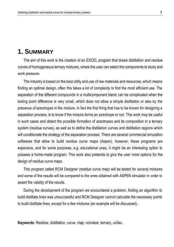
1. SUMMARY
The aim of this work is the creation of an EXCEL program that draws distillation and residue
curves of homogeneous ternary mixtures, where the user can select the components to study and
work pressure.
The industry is based on the best utility and use of raw materials and resources, which means
finding an optimal design, often this takes a lot of complexity to find the most efficient use. The
separation of the different compounds in a multicomponent blend can be complicated when the
boiling point difference is very small, which does not allow a simple distillation or also by the
presence of azeotropes in the mixture. In fact the first thing that has to be known for designing a
separation process, is to know if the mixture forms an azeotrope or not. This work may be useful
in such cases and detect the possible formation of azeotropes and its composition in a ternary
system (residue curves), as well as to define the distillation curves and distillation regions which
will conditionate the strategy of the separation process. There are several commercial simulation
softwares that allow to build residue curve maps (Aspen), however, these programs are
expensive, and for some purposes, e.g. educational ones, it might be an interesting option to
possess a home-made program. This work also pretends to give the user more options for the
design of residue curve maps.
This program called RCM Designer (residue curve map) will be tested for several mixtures
and some of the results will be compared to the ones obtained with ASPEN simulator in order to
assert the validity of the results.
During the development of the program we encountered a problem, finding an algorithm to
build distillate lines was unsuccessful and RCM Designer cannot calculate the necessary points
to build distillate lines, except for a few mixtures (an example will be discussed).
Keywords: Residue, distillation, curve, map, nonideal, ternary, unifac.

Obtaining distillation and residue curves for nonideal ternary systems 5
2. RESUMEN
El tema de este trabajo es la creación de un programa EXCEL que dibuje curvas de
destilación y de residuo de mezclas ternarias homogéneas, de manera que el usuario seleccione
los componentes a estudiar, así como la presión de trabajo.
La industria se basa en la mejor utilidad y aprovechamiento de las materias primas y recursos,
es decir en la búsqueda de un diseño óptimo, esto muchas veces suele llevar una gran
complejidad para encontrar el uso más eficiente. La separación de un sistema multicomponente
en componentes puros puede ser complicada cuando la diferencia de puntos de ebullición es
muy pequeña, lo cual no permite una destilación simple o también por la presencia de azeótropos
en la mezcla. De hecho, lo primero que debe conocerse en el diseño de un proceso de
separación, es saber si la mezcla forma un azeótropo o no. Este trabajo puede ser útil en dichos
casos ya que detecta la posible formación de un azeótropo y su composición en el sistema
ternario (curvas de residuo), también define las líneas de destilación y regiones de destilación
que condicionaran la estrategia del proceso de separación. Existen diversos software
comerciales de simulación que permiten construir mapas de curvas de residuo (Aspen), sin
embargo, estos programas son caros, por ejemplo para uso didáctico puede ser interesante optar
por poseer un programa casero. Este trabajo además pretende darle al usuario más opciones
para diseñar mapas de curvas de residuo.
El programa llamado RCM Designer (diseñador de mapa de curvas de residuo) será puesto
a prueba con diferentes mezclas y algunos de los resultados serán comparados con los obtenidos
mediante el simulador ASPEN para así afirmar la validez de los resultados.
Durante el desarrollo del programa surgió un problema al encontrar un algoritmo que
construyera líneas de destilado por lo cual RCM Designer no puede construirlas exceptuando
algunas mezclas (un ejemplo de esto será discutido).
Palabras clave: Residuo, destilación, curva, mapa, no ideal, ternario, unifac.

Obtaining distillation and residue curves for nonideal ternary systems 7
3. INTRODUCTION
The distillation and residue curves are mainly used as a step in the sequencing of
separation trains because they establish a kind of frontier in which a feed can be separated.
Being this method of study in the mixtures when azeotropes are formed and therefore it’s
required an azeotropic distillation.
As expected, the calculation complexity is conditioned by the number of components
present in the mixture, being able to consider three different cases: binary mixtures, ternary
mixtures or multicomponent mixtures. For binary mixtures, calculation is relatively simple,
widely studied and explained, this can be resolved graphically by McCabe-Thiele or Ponchon-
Savarit methods or analytically by Sorel- Lewis.
For the ternary mixtures, solving equilibrium equations for non-ideal blends is more
complicated. Even when graphical methods can be applied these are not as obvious as it
cannot be represented on a plane of two directions as in binary mixtures, instead it is
necessary working with three-dimensional representations.
Since the case of ternary mixtures will be our topic of study, the subject will be addressed
using projections in a ternary diagram and not three-dimensional representations (set of
multiple projections), this projections work at a given pressure by the user. In the industry,
azeotropic mixtures with more than three compounds are rather unusual.
The calculation methods for ternary mixtures are the same as in the binary mixtures but
its application is not so widely explained for this case and not found in elementary textbooks.
Moreover , since the algebraic resolution of multicomponent systems is the same as for the
ternary mixture calculation can be approached in the same way however It is not possible to
obtain the graphic resolution in multicomponent systems and will not be discussed in this
work .
8 Cruzado Valverde, Héctor
3.1. 1ST RESIDUE CURVE MAP
The study of residue curve maps allow us to detect the azeotropes formed in the mixture
and to know the possible areas of separation and compare the potential separator agents
during the azeotropic or extractive distillation. Although this last use is specific to distillation
curve maps we will use it this way because the trajectories described by the distillation
curves and residue curves of a ternary system are similar in form but not coincident.
For this the use of triangular diagrams allowing us represent residue curves that correspond
to these mixtures at a specified pressure.
A residue curve is the representation of change of composition in the liquid in the boiler
in a simple discontinuous distillation. A set of residue curves (obtained changing the initial
concentration in the bailer), at a given pressure, form a residue curve map.
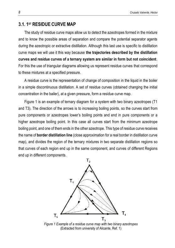
Figure 1 is an example of ternary diagram for a system with two binary azeotropes (T1
and T3). The direction of the arrows is to increasing boiling points, so the curves start from
pure components or azeotropes lower’s boiling points and end in pure components or a
higher azeotrope boiling point. In this case all curves start from the minimum azeotrope
boiling point, and one of them ends in the other azeotrope. This type of residue curve receives
the name of border distillation line (close approximation for a real border in distillation curve
map), and divides the region of the ternary mixtures in two separate distillation regions so
that curves of each region end up in the same component, and curves of different Regions
end up in different components.
Figure 1 Example of a residue curve map with two binary azeotropes (Extracted from university of Alicante, Ref. 1)
Obtaining distillation and residue curves for nonideal ternary systems 9
The interest of these maps lies in the analogy between the composition profiles during
rectification and the curves of simple distillation, providing information on the evolution of the
balance of the system. Moreover, the map’s features determines the validity of a separating
agent for a given separation, being directly related to the sequence of columns and how they
operate.
3.1.1. 2nd Residue Curves
A residue curve is the representation of the evolution of the composition of the residue
over time in a simple distillation.
Its calculation is relatively simple since the curves are only a function of the liquid-vapour
equilibrium and this balance is used to represent the ternary mixtures.
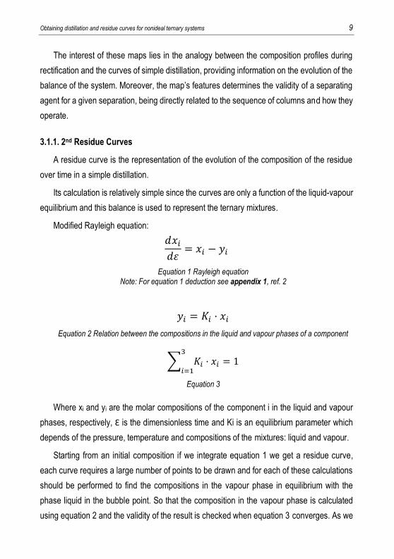
Modified Rayleigh equation:
𝑑𝑥𝑖𝑑𝜀= 𝑥𝑖 − 𝑦𝑖
Equation 1 Rayleigh equation Note: For equation 1 deduction see appendix 1, ref. 2
𝑦𝑖 = 𝐾𝑖 · 𝑥𝑖
Equation 2 Relation between the compositions in the liquid and vapour phases of a component
∑ 𝐾𝑖 · 𝑥𝑖3
𝑖=1= 1
Equation 3
Where xi and yi are the molar compositions of the component i in the liquid and vapour
phases, respectively, Ɛ is the dimensionless time and Ki is an equilibrium parameter which
depends of the pressure, temperature and compositions of the mixtures: liquid and vapour.
Starting from an initial composition if we integrate equation 1 we get a residue curve,
each curve requires a large number of points to be drawn and for each of these calculations
should be performed to find the compositions in the vapour phase in equilibrium with the
phase liquid in the bubble point. So that the composition in the vapour phase is calculated
using equation 2 and the validity of the result is checked when equation 3 converges. As we
10 Cruzado Valverde, Héctor
can see then an iterative calculation is necessary where if equation 3 is not satisfied it will be
repeat the process until it converges.
To a mixture of 3 components have the following variables: T, P, Ɛ, x1, x2, x3, y1, y2, y3.
So we have eight unknown variables and 9 equations (3 from equation 1, 3 from equation 2,
1 from equation 3 and a condition that the sum of x1, x2 and x3 is equal to 1). The equations
are solved by fixing P and introducing an initial concentration in the liquid, and to find the next
point Rayleight equation is integrated with increasing and decreasing intervals of time.
When the integration is done forward in time the curve will eventually end in the less
volatile compound or in a maximum-boiling azeotrope, on the other hand if the integration is
done backwards in time the curve will end in a minimum-boiling azeotrope or in one of the
less volatile compounds.
3.1.2. 2nd Thermodynamic model and considerations
In equation 2, parameter K is function of total pressure, vapour pressures and the activity
coefficients. There are different methods to calculate activity coefficients such as WILSON,
NTRL, UNIQUAC and UNIFAC, being this last method the one used by the program.
3.1.2.1. 3rd UNIFAC model
The UNIFAC model is a semi-empirical method for the prediction of activity coefficients
in non-ideal mixtures. It is based on the group contribution method, using the functional
groups that form each molecule to calculate the activity coefficients, each molecule is
characterized by two structural parameters, a volume parameter r surface parameter q.
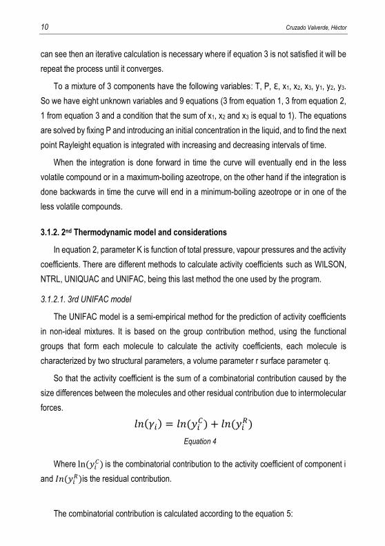
So that the activity coefficient is the sum of a combinatorial contribution caused by the
size differences between the molecules and other residual contribution due to intermolecular
forces.
𝑙𝑛(𝛾𝑖) = 𝑙𝑛(𝑦𝑖𝐶) + 𝑙𝑛(𝑦𝑖
𝑅)
Equation 4
Where ln(𝑦𝑖𝐶) is the combinatorial contribution to the activity coefficient of component i
and 𝐼𝑛(𝑦𝑖𝑅)is the residual contribution.
The combinatorial contribution is calculated according to the equation 5:
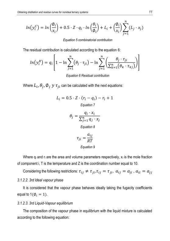
Obtaining distillation and residue curves for nonideal ternary systems 11
𝑙𝑛(𝑦𝑖𝐶) = 𝑙𝑛 (
∅𝑖𝑥𝑖) + 0.5 · 𝑍 · 𝑞𝑖 · 𝑙𝑛 (
𝜃𝑖∅𝑖) + 𝐿𝑖 + (
∅𝑖𝑥𝑖)∑(𝐿𝑗
𝑛
𝑗=1
· 𝑥𝑗)
Equation 5 combinatorial contribution
The residual contribution is calculated according to the equation 6:
𝑙𝑛(𝑦𝑖𝑅) = 𝑞𝑖 [1 − ln∑(𝜃𝑗 · 𝜏𝑗𝑖)
𝑛
𝑗=1
− ln∑(𝜃𝑗 · 𝜏𝑗𝑖
∑ (𝜃𝑘 · 𝜏𝑘𝑗)𝑛𝑘=1
)
𝑛
𝑗=1
]
Equation 6 Residual contribution
Where 𝐿𝑖 , 𝜃𝑗 , ∅𝑗𝑦𝜏𝑗𝑖 can be calculated with the next equations:
𝐿𝑖 = 0.5 · 𝑍 · (𝑟𝑖 − 𝑞𝑖) − 𝑟𝑖 + 1
Equation 7
𝜃𝑗 =𝑞𝑖 · 𝑥𝑖
∑ 𝑞𝑗 · 𝑥𝑗𝑛𝑗=1
Equation 8
𝜏𝑗𝑖 =𝑎𝑖𝑗
𝑅𝑇
Equation 9
Where qi and ri are the area and volume parameters respectively, x i is the mole fraction
of component i, T is the temperature and Z is the coordination number equal to 10.
Considering the following restrictions: 𝜏𝑖𝑗 ≠ 𝜏𝑗𝑖 ,𝜏𝑖𝑗 = 𝜏𝑗𝑖, 𝑎𝑖𝑗 = 𝑎𝑗𝑖 , 𝑎𝑖𝑖 = 𝑎𝑗𝑗
3.1.2.2. 3rd Ideal vapour phase
It is considered that the vapour phase behaves ideally taking the fugacity coefficients
equal to 1(∅𝑖 = 1).
3.1.2.3. 3rd Liquid-Vapour equilibrium
The composition of the vapour phase in equilibrium with the liquid mixture is calculated
according to the following equation:
12 Cruzado Valverde, Héctor
Figure 2 Stable node (Reproduced from university of Alicante, Ref. 1)
𝑦𝑖 =𝑥𝑖 · 𝛾𝑖 · 𝑃𝑖
𝑠𝑎𝑡
𝑃
Equation 10
3.1.2.4. 3rd Vapour pressure
The vapour pressure can be calculated with the extended Antoine equation:
𝑙𝑛(𝑃𝑠𝑎𝑡) = 𝐴 ∗ 𝐿𝑜𝑔(𝑇) + 𝐵/𝑇 + 𝐶 + 𝐷 ∗ 𝑇2)
Equation 11 Extended Antoine equation
Where T is the temperature, and the values of A, B, C and D are specific of each
component, giving the result in mmHg.
3.1.3. 2nd Features of residue curve maps
In a triangular diagram, all vertices (pure components) and the points where the
azeotropes are represented are singular points or fixed points of the residue curves because
in these points dx/dƐ=0.
Three different cases can be presented in a residue curve map.
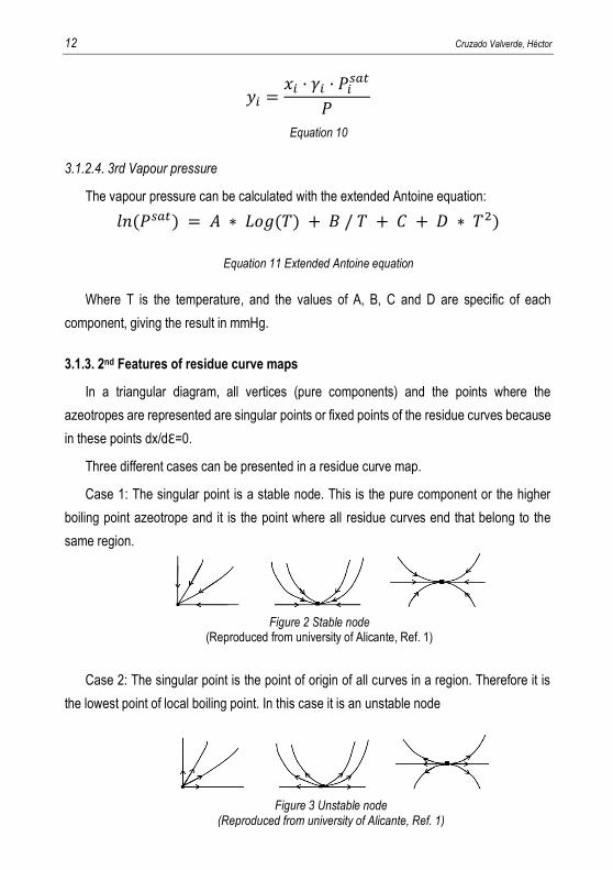
Case 1: The singular point is a stable node. This is the pure component or the higher
boiling point azeotrope and it is the point where all residue curves end that belong to the
same region.
Case 2: The singular point is the point of origin of all curves in a region. Therefore it is
the lowest point of local boiling point. In this case it is an unstable node
Figure 3 Unstable node (Reproduced from university of Alicante, Ref. 1)
Obtaining distillation and residue curves for nonideal ternary systems 13
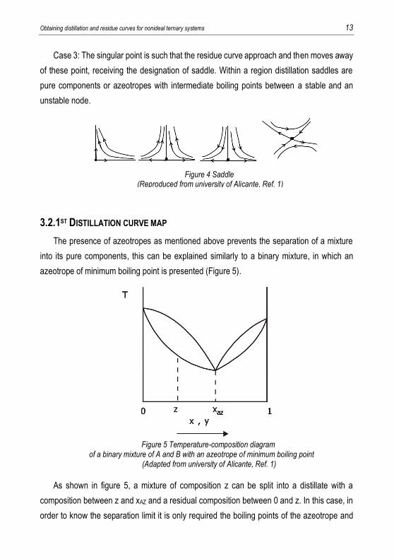
Case 3: The singular point is such that the residue curve approach and then moves away
of these point, receiving the designation of saddle. Within a region distillation saddles are
pure components or azeotropes with intermediate boiling points between a stable and an
unstable node.
3.2.1ST DISTILLATION CURVE MAP
The presence of azeotropes as mentioned above prevents the separation of a mixture
into its pure components, this can be explained similarly to a binary mixture, in which an
azeotrope of minimum boiling point is presented (Figure 5).
As shown in figure 5, a mixture of composition z can be split into a distillate with a
composition between z and xAZ and a residual composition between 0 and z. In this case, in
order to know the separation limit it is only required the boiling points of the azeotrope and
Figure 4 Saddle (Reproduced from university of Alicante, Ref. 1)
Figure 5 Temperature-composition diagram of a binary mixture of A and B with an azeotrope of minimum boiling point
(Adapted from university of Alicante, Ref. 1) .
14 Cruzado Valverde, Héctor
pure components and the azeotrope’s concentration. However for a ternary mixture is not so
simple, though the same information is required and the composition obtained depends on
the initial concentration in the ternary diagram too, when there is an azeotrope the
composition profiles in a rectifying column cannot go any zone but it is limited by internal
borders (distillation border) that divide the diagram into different zones (distillation regions).
It is necessary to know these boundaries, otherwise when there are actual azeotropes, a
distillation problem for ternary mixtures can’t be solved correctly.
Recently, an application for binary mixtures with azeotropes has been reported, known as
assisted distillation in which a separator agent allows separate the initial components in
concentrations that could not be achieved by ordinary distillation. [Note: information obtained
from ref. 1]
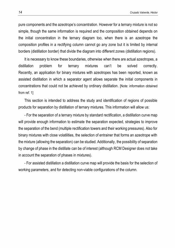
This section is intended to address the study and identification of regions of possible
products for separation by distillation of ternary mixtures. This information will allow us:
- For the separation of a ternary mixture by standard rectification, a distillation curve map
will provide enough information to estimate the separation expected, strategies to improve
the separation of the bend (multiple rectification towers and their working pressures). Also for
binary mixtures with close volatilities, the selection of entrainer that forms an azeotrope with
the mixture (allowing the separation) can be studied. Additionally, the possibility of separation
by change of phase in the distillate can be of interest (although RCM Designer does not take
in account the separation of phases in mixtures).
- For assisted distillation a distillation curve map will provide the basis for the selection of
working parameters, and for detecting non-viable configurations of the column.
Obtaining distillation and residue curves for nonideal ternary systems 15
3.2.1 2nd Distillation curves
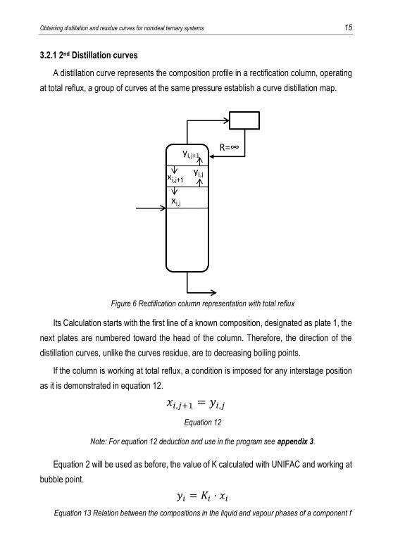
A distillation curve represents the composition profile in a rectification column, operating
at total reflux, a group of curves at the same pressure establish a curve distillation map.
Its Calculation starts with the first line of a known composition, designated as plate 1, the
next plates are numbered toward the head of the column. Therefore, the direction of the
distillation curves, unlike the curves residue, are to decreasing boiling points.
If the column is working at total reflux, a condition is imposed for any interstage position
as it is demonstrated in equation 12.
𝑥𝑖,𝑗+1 = 𝑦𝑖,𝑗
Equation 12
Note: For equation 12 deduction and use in the program see appendix 3.
Equation 2 will be used as before, the value of K calculated with UNIFAC and working at
bubble point.
𝑦𝑖 = 𝐾𝑖 · 𝑥𝑖
Equation 13 Relation between the compositions in the liquid and vapour phases of a component f
Figure 6 Rectification column representation with total reflux
16 Cruzado Valverde, Héctor
3.2.2 2nd Thermodynamic model and considerations
The equations used will be same as in the previous section (residue curves). So the
UNIFAC method will be used to estimate the activity, considering the behaviour of the vapour
phase as ideal. Also the liquid-vapour equilibrium and bubble pressure will be calculated as
before (equations 10 and 11, respectively).
3.2.3 2nd Distillation borders
Distillation borders appear as a result of the changes in the relative volatility in ternary
mixtures due to the presence of azeotrope’s boiling points.
A study of these borders show that they must meet the following condition:
- The relative volatilities of the two components along the border tend to be equal to
1, because when passing through the border, a reversal of the volatility will occur.
Of great interest is the effect of distillation boundaries on the operation of distillation
towers. To summarize a growing body of literature, it is well established that the composition
of a distillation tower operating at total reflux cannot cross the distillation-line boundaries,
except under unusual circumstances, where these boundaries exhibit a high degree of
curvature. This provides the total-reflux bound on the possible (feasible) compositions for the
distillate and bottoms products. [“Product & Process Design Principles” p. 269, ref. 2]
4. OBJECTIVES
- The objective of this work is to build a computer program using Excel that draws
distillation and residue curve maps of components selected by the user.
- The program will show possible azeotropes in the mixture and its nature (maximum or
minimum boiling point, or saddle).
- Validate the results using a commercial simulator and data found experimentally.
Obtaining distillation and residue curves for nonideal ternary systems 17
5. DEVELOPMENT: RCM DESIGNER
In order to create the program, this project will follow four basic steps: bibliography review,
election of the algorithm, codification, and validation of the results.
5.1 1ST BIBLIOGRAPHY REVIEW
Selection of the thermodynamic model, in this case UNIFAC model (equations 4 to 9).
Also it is selected the equations that will be used in the calculation of pure components
and ternary mixtures, these are presented in the introduction (equations 1, 2, 3, 10 and 11).
Selection of different compounds to study, using the data base from CHERIC (Chemical
Engineering Research Information Center).
5.2 1ST ELECTION OF THE ALGORITHM
This section it’s focus in the development of a simple algorithm for the construction of
residue curve maps, using the proper equations for plotting residue curves and for the
thermodynamic model. The process’s mathematical model used in the program involves the
equations for vapour-liquid equilibrium, the extended Antoine equation (Equation 11) for the
calculation of the vapour pressures and the equations present in the thermodynamic model
UNIFAC (Equations 4 to 9). The database CHERIC will be used to obtain the parameters for
the Antoine equation.
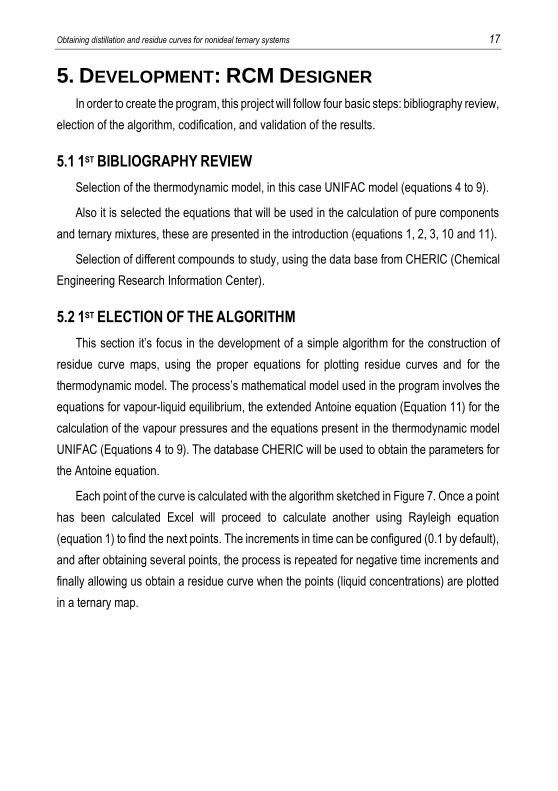
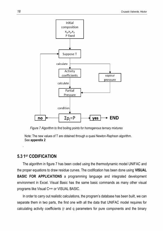
Each point of the curve is calculated with the algorithm sketched in Figure 7. Once a point
has been calculated Excel will proceed to calculate another using Rayleigh equation
(equation 1) to find the next points. The increments in time can be configured (0.1 by default),
and after obtaining several points, the process is repeated for negative time increments and
finally allowing us obtain a residue curve when the points (liquid concentrations) are plotted
in a ternary map.
18 Cruzado Valverde, Héctor
.
5.3 1ST CODIFICATION
The algorithm in figure 7 has been coded using the thermodynamic model UNIFAC and
the proper equations to draw residue curves. The codification has been done using VISUAL
BASIC FOR APPLICATIONS a programming language and integrated development
environment in Excel. Visual Basic has the same basic commands as many other visual
programs like Visual C++ or VISUAL BASIC.
In order to carry out realistic calculations, the program’s database has been built, we can
separate them in two parts, the first one with all the data that UNIFAC model requires for
calculating activity coefficients (r and q parameters for pure components and the binary
Figure 7 Algorithm to find boiling points for homogenous ternary mixtures
Note: The new values of T are obtained through a quasi Newton-Raphson algorithm. See appendix 2
Obtaining distillation and residue curves for nonideal ternary systems 19
interaction parameters). The second data base contains Antoine’s equation constants
required for calculating vapour pressure.
Note: UNIFAC model has been coded by Dr. David Curcó Cantarell (Department of
Chemistry Engineering, University of Barcelona).
5.4 1ST VALIDATION OF THE RESULTS
In order to check if the residue curve maps plotted represent correctly the reality with its
stable and unstable nodes and saddles, we compare with maps created with Aspen Plus, an
AspenTech simulator. Aspen Plus is a recognized software created to simulate and design
distillation columns and it has an application for drawing residue curve maps.
For this we need to vary the work conditions for both programs and evaluate the response
for this changes. It is known that the mixture’s behaviour varies depending on the system
pressure, because it affects the molecule interaction of the components, and hence their
relative volatility. With the intention of observing the software’s accuracy in the calculation
and plotting of residue curve maps at different pressures, different maps were built, the results
being compared with those calculated by Aspen.
The comparison criteria will be the trends and location of the different nodes (stable,
unstable or saddle) at different pressures keeping the same initial compositions for both
programs.
20 Cruzado Valverde, Héctor
6. RESULTS AND DISCUSSION
6.1 1ST SECTIONS OF THE PROGRAM
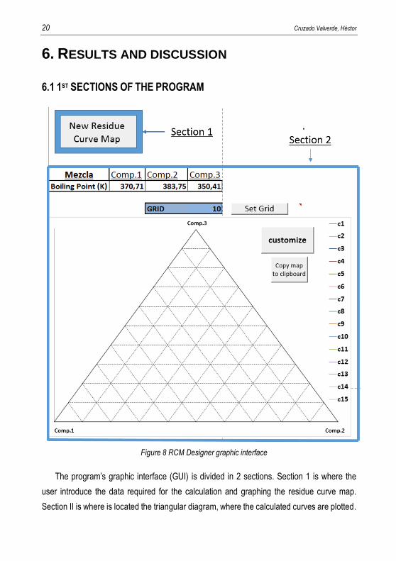
The program’s graphic interface (GUI) is divided in 2 sections. Section 1 is where the
user introduce the data required for the calculation and graphing the residue curve map.
Section II is where is located the triangular diagram, where the calculated curves are plotted.
Figure 8 RCM Designer graphic interface
Obtaining distillation and residue curves for nonideal ternary systems 21
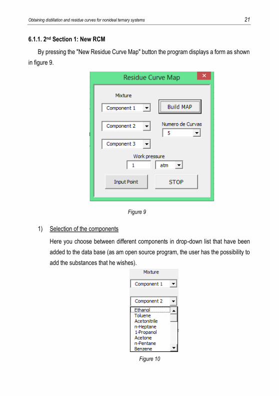
6.1.1. 2nd Section 1: New RCM
By pressing the "New Residue Curve Map" button the program displays a form as shown
in figure 9.
1) Selection of the components
Here you choose between different components in drop-down list that have been
added to the data base (as am open source program, the user has the possibility to
add the substances that he wishes).
Figure 9
Figure 10
22 Cruzado Valverde, Héctor
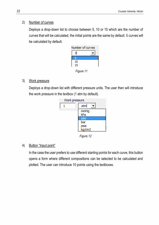
2) Number of curves
Deploys a drop-down list to choose between 5, 10 or 15 which are the number of
curves that will be calculated, the initial points are the same by default. 5 curves will
be calculated by default.
3) Work pressure
Deploys a drop-down list with different pressure units. The user then will introduce
the work pressure in the textbox (1 atm by default).
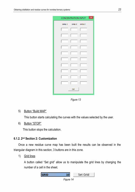
4) Button “Input point”
In the case the user prefers to use different starting points for each curve, this button
opens a form where different compositions can be selected to be calculated and
plotted. The user can introduce 10 points using the textboxes.
Figure 11
Figure 12
Obtaining distillation and residue curves for nonideal ternary systems 23
5) Button “Build MAP”
This button starts calculating the curves with the values selected by the user.
6) Button “STOP”
This button stops the calculation.
6.1.2. 2nd Section 2: Customization
Once a new residue curve map has been built the results can be observed in the
triangular diagram in this section, 3 buttons are in this zone.
1) Grid lines
A button called “Set grid” allow us to manipulate the grid lines by changing the
number of a cell in the sheet.
Figure 13
Figure 14
24 Cruzado Valverde, Héctor
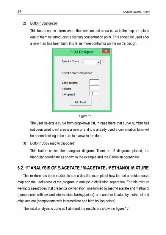
2) Button “Customize”
This button opens a form where the user can add a new curve to the map or replace
one of them by introducing a starting concentration point. This should be used after
a new map has been built, this let us more control for on the map’s design.
The user selects a curve from drop-down list, in case there that curve number has
not been used it will create a new one, if it is already used a confirmation form will
be opened asking to be sure to overwrite the data.
3) Button “Copy map to clipboard”
This button copies the triangular diagram. There are 2 diagrams plotted, the
triangular coordinate as shown in the example and the Cartesian coordinate.
6.2. 1ST ANALYSIS OF E-ACETATE / M-ACETATE / METHANOL MIXTURE
This mixture has been studied to see a detailed example of how to read a residue curve
map and the usefulness of the program to analyse a distillation separation. For this mixture
we find 2 azeotropes that present a low variation, one formed by methyl acetate and methanol
(components with low and intermediate boiling points), and another located by methanol and
ethyl acetate (components with intermediate and high boiling points).
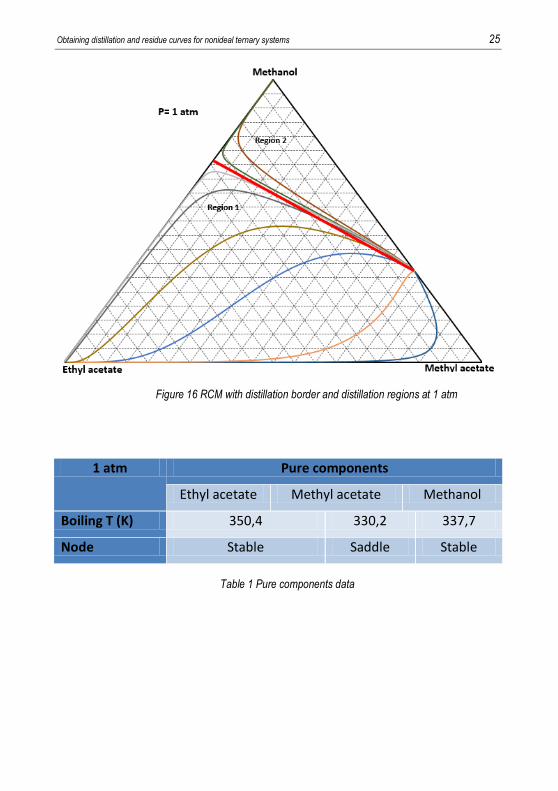
The initial analysis is done at 1 atm and the results are shown in figure 16.
Figure 15
Obtaining distillation and residue curves for nonideal ternary systems 25
Table 1 Pure components data
1 atm Pure components
Ethyl acetate Methyl acetate Methanol
Boiling T (K) 350,4 330,2 337,7
Node Stable Saddle Stable
Figure 16 RCM with distillation border and distillation regions at 1 atm

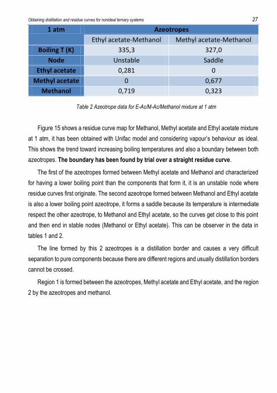
Obtaining distillation and residue curves for nonideal ternary systems 27
1 atm Azeotropes
Ethyl acetate-Methanol Methyl acetate-Methanol
Boiling T (K) 335,3 327,0
Node Unstable Saddle
Ethyl acetate 0,281 0
Methyl acetate 0 0,677
Methanol 0,719 0,323
Figure 15 shows a residue curve map for Methanol, Methyl acetate and Ethyl acetate mixture
at 1 atm, it has been obtained with Unifac model and considering vapour’s behaviour as ideal.
This shows the trend toward increasing boiling temperatures and also a boundary between both
azeotropes. The boundary has been found by trial over a straight residue curve.
The first of the azeotropes formed between Methyl acetate and Methanol and characterized
for having a lower boiling point than the components that form it, it is an unstable node where
residue curves first originate. The second azeotrope formed between Methanol and Ethyl acetate
is also a lower boiling point azeotrope, it forms a saddle because its temperature is intermediate
respect the other azeotrope, to Methanol and Ethyl acetate, so the curves get close to this point
and then end in stable nodes (Methanol or Ethyl acetate). This can be observer in the data in
tables 1 and 2.
The line formed by this 2 azeotropes is a distillation border and causes a very difficult
separation to pure components because there are different regions and usually distillation borders
cannot be crossed.
Region 1 is formed between the azeotropes, Methyl acetate and Ethyl acetate, and the region
2 by the azeotropes and methanol.
Table 2 Azeotrope data for E-Ac/M-Ac/Methanol mixture at 1 atm
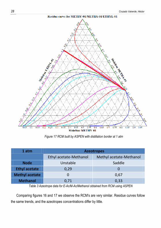
28 Cruzado Valverde, Héctor
1 atm Azeotropes
Ethyl acetate-Methanol Methyl acetate-Methanol
Node Unstable Saddle
Ethyl acetate 0,29 0
Methyl acetate 0 0,67
Methanol 0,71 0,33 Table 3 Azeotrope data for E-Ac/M-Ac/Methanol obtained from RCM using ASPEN
Comparing figures 16 and 17 we observe the RCM’s are very similar. Residue curves follow
the same trends, and the azeotropes concentrations differ by little.
Figure 17 RCM built by ASPEN with distillation border at 1 atm
Obtaining distillation and residue curves for nonideal ternary systems 29
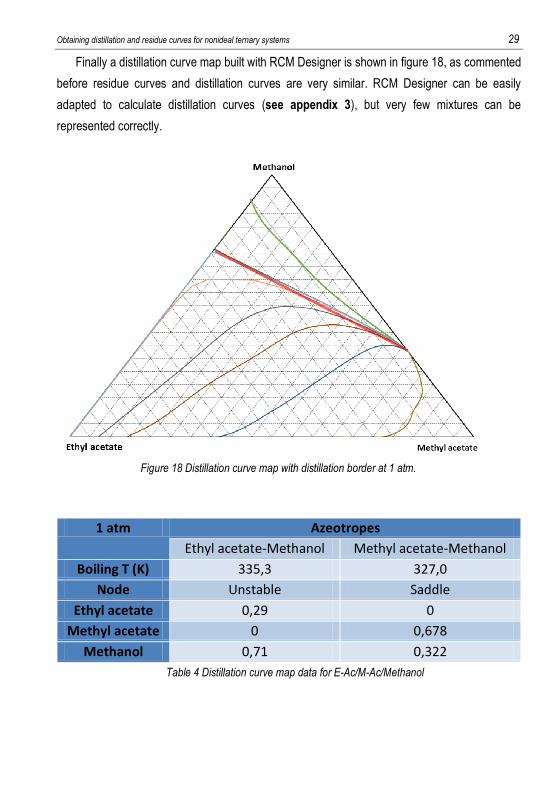
Finally a distillation curve map built with RCM Designer is shown in figure 18, as commented
before residue curves and distillation curves are very similar. RCM Designer can be easily
adapted to calculate distillation curves (see appendix 3), but very few mixtures can be
represented correctly.
1 atm Azeotropes
Ethyl acetate-Methanol Methyl acetate-Methanol
Boiling T (K) 335,3 327,0
Node Unstable Saddle
Ethyl acetate 0,29 0
Methyl acetate 0 0,678
Methanol 0,71 0,322
Table 4 Distillation curve map data for E-Ac/M-Ac/Methanol
Figure 18 Distillation curve map with distillation border at 1 atm.
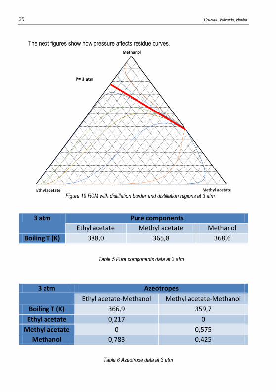
30 Cruzado Valverde, Héctor
The next figures show how pressure affects residue curves.
3 atm Pure components
Ethyl acetate Methyl acetate Methanol
Boiling T (K) 388,0 365,8 368,6
Table 5 Pure components data at 3 atm
Table 6 Azeotrope data at 3 atm
3 atm Azeotropes
Ethyl acetate-Methanol Methyl acetate-Methanol
Boiling T (K) 366,9 359,7
Ethyl acetate 0,217 0
Methyl acetate 0 0,575
Methanol 0,783 0,425
Figure 19 RCM with distillation border and distillation regions at 3 atm
Obtaining distillation and residue curves for nonideal ternary systems 31
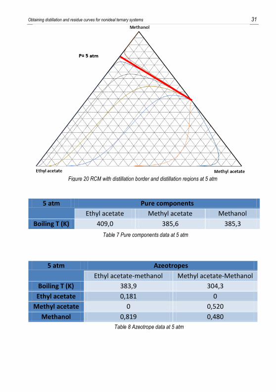
Table 7 Pure components data at 5 atm
5 atm Pure components
Ethyl acetate Methyl acetate Methanol
Boiling T (K) 409,0 385,6 385,3
Table 8 Azeotrope data at 5 atm
5 atm Azeotropes
Ethyl acetate-methanol Methyl acetate-Methanol
Boiling T (K) 383,9 304,3
Ethyl acetate 0,181 0
Methyl acetate 0 0,520
Methanol 0,819 0,480
Figure 20 RCM with distillation border and distillation regions at 5 atm
32 Cruzado Valverde, Héctor
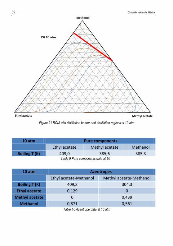
10 atm Azeotropes
Ethyl acetate-Methanol Methyl acetate-Methanol
Boiling T (K) 409,8 304,3
Ethyl acetate 0,129 0
Methyl acetate 0 0,439
Methanol 0,871 0,561 Table 10 Azeotrope data at 10 atm
10 atm Pure components
Ethyl acetate Methyl acetate Methanol
Boiling T (K) 409,0 385,6 385,3 Table 9 Pure components data at 10
Figure 21 RCM with distillation border and distillation regions at 10 atm
Obtaining distillation and residue curves for nonideal ternary systems 33
As shown in in figures 19, 20 and 21 changing the system’s pressure modifies the residue
curve map, in this case we can observe how the distillation border moves, because with increasing
pressures Ethyl acetate-Methanol azeotrope change its composition approximating to the pure
methanol node. Observing how pressure affects the system we can affirm that it is possible to
brake this azeotrope at very high pressures. So pressure modifies residue curves, azeotrope’s
compositions and also distillation borders and its curvature, because of this RCM’s are so
important, they define the ranges where a mixture can be separated with each distillation
sequence.
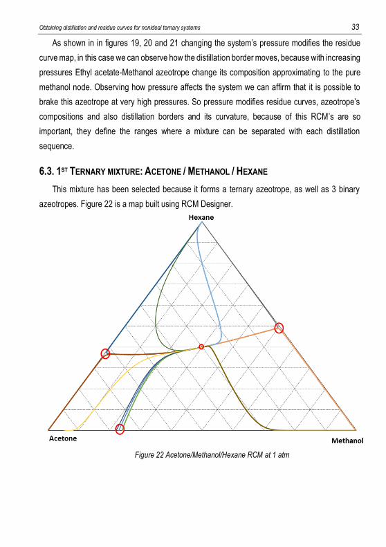
6.3. 1ST TERNARY MIXTURE: ACETONE / METHANOL / HEXANE
This mixture has been selected because it forms a ternary azeotrope, as well as 3 binary
azeotropes. Figure 22 is a map built using RCM Designer.
Figure 22 Acetone/Methanol/Hexane RCM at 1 atm
34 Cruzado Valverde, Héctor
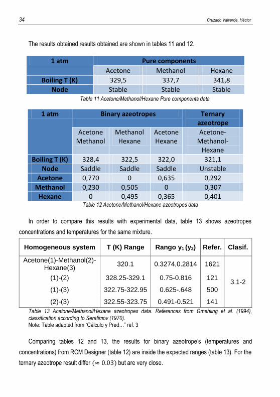
The results obtained results obtained are shown in tables 11 and 12.
1 atm Binary azeotropes Ternary azeotrope
Acetone Methanol
Methanol Hexane
Acetone Hexane
Acetone-Methanol-
Hexane
Boiling T (K) 328,4 322,5 322,0 321,1
Node Saddle Saddle Saddle Unstable
Acetone 0,770 0 0,635 0,292
Methanol 0,230 0,505 0 0,307
Hexane 0 0,495 0,365 0,401 Table 12 Acetone/Methanol/Hexane azeotropes data
In order to compare this results with experimental data, table 13 shows azeotropes
concentrations and temperatures for the same mixture.
Homogeneous system T (K) Range Rango y1 (y2) Refer. Clasif.
Acetone(1)-Methanol(2)-Hexane(3)
320.1 0.3274,0.2814 1621
3.1-2 (1)-(2) 328.25-329.1 0.75-0.816 121
(1)-(3) 322.75-322.95 0.625-.648 500
(2)-(3) 322.55-323.75 0.491-0.521 141
Table 13 Acetone/Methanol/Hexane azeotropes data. References from Gmehling et al. (1994), classification according to Serafimov (1970). Note: Table adapted from “Cálculo y Pred…” ref. 3
Comparing tables 12 and 13, the results for binary azeotrope’s (temperatures and
concentrations) from RCM Designer (table 12) are inside the expected ranges (table 13). For the
ternary azeotrope result differ (≈ 0.03) but are very close.
1 atm Pure components
Acetone Methanol Hexane
Boiling T (K) 329,5 337,7 341,8
Node Stable Stable Stable Table 11 Acetone/Methanol/Hexane Pure components data
Obtaining distillation and residue curves for nonideal ternary systems 35
7. CONCLUSIONS
Comparing the results obtained with ASPEN we can assert that RCM Designer is consistent,
because residue curves show the same trends, forms, the same nodes and also changes in the
working pressure affect both programs similarly.
RCM Designer has limitations to predict some ternary azeotropes due to the thermodynamic
model used, the program cannot predict azeotropes for some mixtures where alcohols are present
(propanol for example).
The program, in most cases is not able to plot distillation curves since the algorithm necessary
for it is complicated, nevertheless RCM can be adapted (see appendix 3) to calculate distillation
curves but the necessary points to be plotted are insufficient for the majority of mixtures. As a
recommendation for future works, the development of an algorithm specific for distillation curves
would be necessary.

Obtaining distillation and residue curves for nonideal ternary systems 37
8. REFERENCES AND NOTES 1. Amparo Gómez siurana, Alicia Font Escamilla, Antonio Marcilla Gomis. Universidad de Alicante. Dpto.
Ingeniería Química: Ampliación de Operaciones de Separación. http://iq.ua.es/Destilacion/ (accessed Feb 25, 2014).
2. Warren D Seider, Junior D Seader, Daniel R Lewin. Product & Process Design Principles: Synthesis, Analysis and Evaluation, 2nd ed.;John Wiley & Sons: New York, 1999, pp 259-282.
3. Lorenz T. Biegler, Ignacio E. Grossmann, Arthur W. Westerberg. Systematic methods of chemical process design; Prentice Hall PTR, 1997.
4. MANDAGARAN, Beatriz A y CAMPANELLA, Enrique A. Cálculo y Predicción de Azeótropos Multicomponentes con Modelos de Coeficientes de Actividad. Inf. tecnol. [Online]. 2008, vol.19, n.5, pp. 73-84. ISSN 0718-0764. http://dx.doi.org/10.4067/S0718-07642008000500009 (accessed Nov 10, 2014).

Obtaining distillation and residue curves for nonideal ternary systems 39
APPENDICES

Obtaining distillation and residue curves for nonideal ternary systems 41
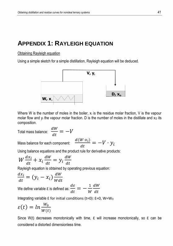
APPENDIX 1: RAYLEIGH EQUATION
Obtaining Rayleigh equation
Using a simple sketch for a simple distillation, Rayleigh equation will be deduced.
Where W is the number of moles in the boiler, x i is the residue molar fraction, V is the vapour molar flow and yi the vapour molar fraction. D is the number of moles in the distillate and xD its composition.
Total mass balance: 𝑑𝑊
𝑑𝑡= −𝑉
Mass balance for each component: 𝑑(𝑊·𝑥𝑖)
𝑑𝑡= −𝑉 · 𝑦𝑖
Using balance equations and the product rule for derivative products:
𝑊𝑑𝑥𝑖
𝑑𝑡+ 𝑥𝑖
𝑑𝑊
𝑑𝑡= 𝑦𝑖
𝑑𝑊
𝑑𝑡
Rayleigh equation is obtained by operating previous equation:
𝑑𝑥𝑖
𝑑𝑡= (𝑦𝑖 − 𝑥𝑖)
𝑑𝑊
𝑊𝑑𝑡
We define variable Ɛ is defined as: 𝑑𝜀
𝑑𝑡= −
1
𝑊
𝑑𝑊
𝑑𝑡
Integrating variable Ɛ for initial conditions (t=0): Ɛ=0, W=W0
𝜀(𝑡) = 𝑙𝑛𝑊0
𝑊(𝑡)
Since W(t) decreases monotonically with time, Ɛ will increase monotonically, so Ɛ can be
considered a distorted dimensionless time.
42 Cruzado Valverde, Héctor
Introducing variable Ɛ in Rayleigh equation and operating, we obtain the extended Rayleigh
equation used in the program.
𝑑𝑥𝑖
𝑑𝜀= (𝑦𝑖 − 𝑥𝑖)
Obtaining distillation and residue curves for nonideal ternary systems 43
APPENDIX 2: NEWTON-RAPHSON METHOD
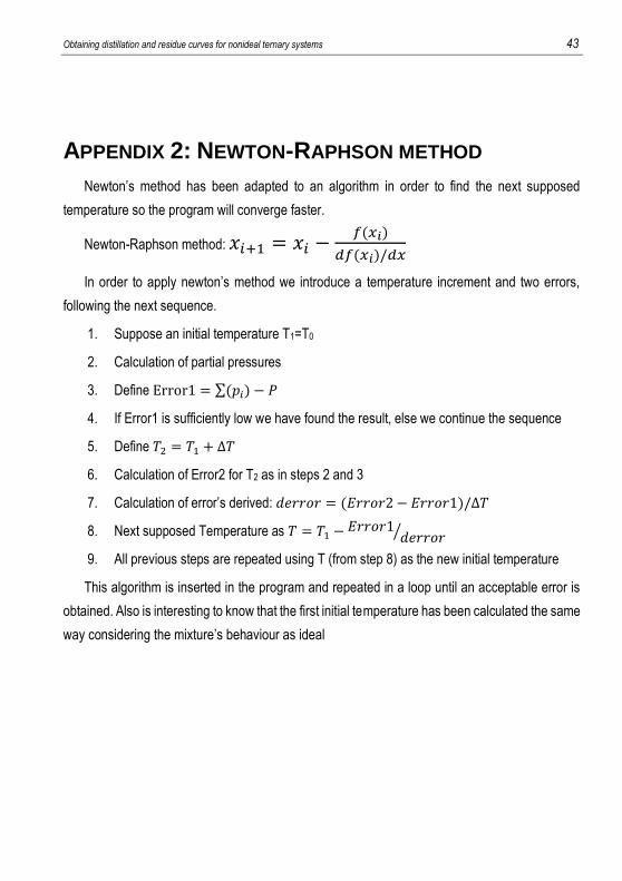
Newton’s method has been adapted to an algorithm in order to find the next supposed
temperature so the program will converge faster.
Newton-Raphson method: 𝑥𝑖+1 = 𝑥𝑖 −𝑓(𝑥𝑖)
𝑑𝑓(𝑥𝑖)/𝑑𝑥
In order to apply newton’s method we introduce a temperature increment and two errors,
following the next sequence.
1. Suppose an initial temperature T1=T0
2. Calculation of partial pressures
3. Define Error1 = ∑(𝑝𝑖) − 𝑃
4. If Error1 is sufficiently low we have found the result, else we continue the sequence
5. Define 𝑇2 = 𝑇1 + ∆𝑇
6. Calculation of Error2 for T2 as in steps 2 and 3
7. Calculation of error’s derived: 𝑑𝑒𝑟𝑟𝑜𝑟 = (𝐸𝑟𝑟𝑜𝑟2 − 𝐸𝑟𝑟𝑜𝑟1)/∆𝑇
8. Next supposed Temperature as 𝑇 = 𝑇1 −𝐸𝑟𝑟𝑜𝑟1
𝑑𝑒𝑟𝑟𝑜𝑟⁄
9. All previous steps are repeated using T (from step 8) as the new initial temperature
This algorithm is inserted in the program and repeated in a loop until an acceptable error is
obtained. Also is interesting to know that the first initial temperature has been calculated the same
way considering the mixture’s behaviour as ideal

Títol. Si és massa llarg cal truncar-lo i posar punts suspensius... 45
APPENDIX 3: RCM DESIGNER AND DISTILLATION
CURVES
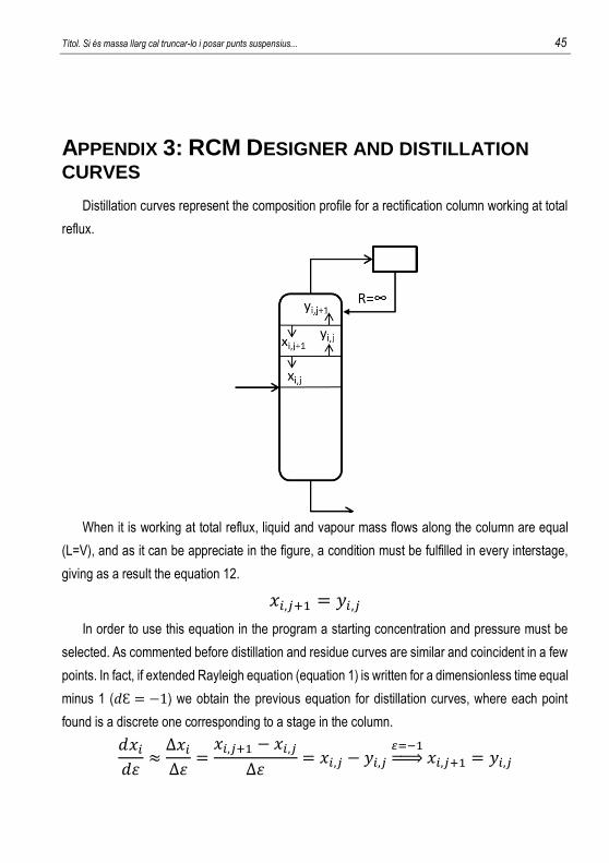
Distillation curves represent the composition profile for a rectification column working at total
reflux.
When it is working at total reflux, liquid and vapour mass flows along the column are equal
(L=V), and as it can be appreciate in the figure, a condition must be fulfilled in every interstage,
giving as a result the equation 12.
𝑥𝑖,𝑗+1 = 𝑦𝑖,𝑗
In order to use this equation in the program a starting concentration and pressure must be
selected. As commented before distillation and residue curves are similar and coincident in a few
points. In fact, if extended Rayleigh equation (equation 1) is written for a dimensionless time equal
minus 1 (𝑑Ɛ = −1) we obtain the previous equation for distillation curves, where each point
found is a discrete one corresponding to a stage in the column.
𝑑𝑥𝑖𝑑𝜀≈∆𝑥𝑖∆𝜀=𝑥𝑖,𝑗+1 − 𝑥𝑖,𝑗
∆𝜀= 𝑥𝑖,𝑗 − 𝑦𝑖,𝑗
𝜀=−1⇒ 𝑥𝑖,𝑗+1 = 𝑦𝑖,𝑗