Embed Size (px)
Citation preview

Treball Final de Grau
Tutor/s
Dr. Manel Vicente Chemical engineering department
Dr. Jose Maria Gutiérrez Chemical engineering department
Production scheduling of multipurpose batch plants. Application to a case of production plant for active pharmaceutical ingredients (API’s).
Programació de la producció en plantes discontinues multi propòsit. Aplicació a un cas de una planta de producció de principis actius (API’s)
Bernat Rosa Serrat January of 2014

Aquesta obra esta subjecta a la llicència de: Reconeixement–NoComercial-SenseObraDerivada
http://creativecommons.org/licenses/by-nc-nd/3.0/es/

There is a theory which states that if ever anyone discovers exactly what the
Universe is for and why it is here, it will instantly disappear and be replaced
by something even more bizarre and inexplicable.
-The hitchhiker’s guide to galaxy


REPORT

Production scheduling of multipurpose batch plants. Application to a case of production plant for active pharmaceutical ingredients 1
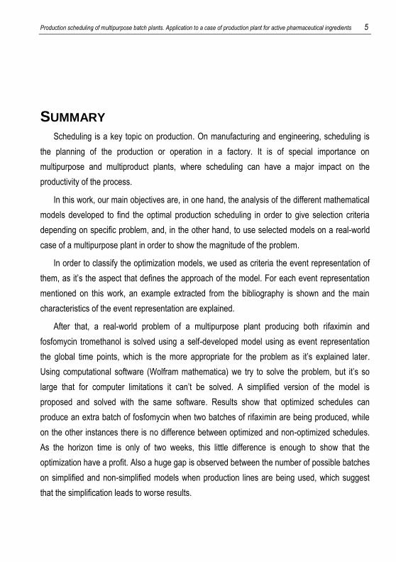
CONTENTS
SUMMARY 5
RESUM 7
INTRODUCTION 9
OBJECTIVES 12
OPTIMIZATION MODELS 12
CLASSIFICATION OF OPTIMIZATION MODELS 13
Time representation 13
Material balances 14
Event representation 14
Objective function 17
MODELING ASPECTS OF OPTIMIZATION MODELS 17
Global time intervals 18
Global time points 19
Unit-specific time events 21
Time slots 25
Unit-specific immediate precedence 26
Immediate precedence 27
General precedence 28
THE REAL CASE 30
THE PROCESS 30
MODELING ASPECTS OF THE PROCESS 34
Simplified model 37
RESULTS 38
CONCLUSIONS 43

REFERENCES AND NOTES 45
APPENDICES 47
APPENDIX 1: SORT DESCRIPTIVE TITLE 49
APPENDIX 2: SORT DESCRIPTIVE TITLE 23

Production scheduling of multipurpose batch plants. Application to a case of production plant for active pharmaceutical ingredients 3

Production scheduling of multipurpose batch plants. Application to a case of production plant for active pharmaceutical ingredients 5
SUMMARY
Scheduling is a key topic on production. On manufacturing and engineering, scheduling is
the planning of the production or operation in a factory. It is of special importance on
multipurpose and multiproduct plants, where scheduling can have a major impact on the
productivity of the process.
In this work, our main objectives are, in one hand, the analysis of the different mathematical
models developed to find the optimal production scheduling in order to give selection criteria
depending on specific problem, and, in the other hand, to use selected models on a real-world
case of a multipurpose plant in order to show the magnitude of the problem.
In order to classify the optimization models, we used as criteria the event representation of
them, as it’s the aspect that defines the approach of the model. For each event representation
mentioned on this work, an example extracted from the bibliography is shown and the main
characteristics of the event representation are explained.
After that, a real-world problem of a multipurpose plant producing both rifaximin and
fosfomycin tromethanol is solved using a self-developed model using as event representation
the global time points, which is the more appropriate for the problem as it’s explained later.
Using computational software (Wolfram mathematica) we try to solve the problem, but it’s so
large that for computer limitations it can’t be solved. A simplified version of the model is
proposed and solved with the same software. Results show that optimized schedules can
produce an extra batch of fosfomycin when two batches of rifaximin are being produced, while
on the other instances there is no difference between optimized and non-optimized schedules.
As the horizon time is only of two weeks, this little difference is enough to show that the
optimization have a profit. Also a huge gap is observed between the number of possible batches
on simplified and non-simplified models when production lines are being used, which suggest
that the simplification leads to worse results.

Production scheduling of multipurpose batch plants. Application to a case of production plant for active pharmaceutical ingredients 7
RESUM
Un aspecte clau en la producció és la programació de la operació o producció en fàbrica.
És d’especial importància en plantes multi producte i multi propòsit , on la programació de la
producció pot tenir un efecte important en la productivitat del procés.
En aquest treball, els principals objectius son, per una part, el anàlisis de diferents models
matemàtics desenvolupats per altres autors que busquen la programació òptima d’una planta i,
per l’altre banda, desenvolupar el nostre propi model per a un cas real i mostrar la magnitud
d’aquest tipus de problemes.
Els models d’optimització s’han classificat segons el tipus de representació
d’esdeveniments que utilitzen, ja que és l’aspecte que defineix l’estratègia per abordar el
problema. Per cada tipus de representació d’esdeveniments mencionat en aquest treball es
mostra un model matemàtic que l’utilitza com a exemple, i s’expliquen les seves principals
característiques.
A continuació, s’aborda la programació de una planta multi propòsit que produeix rifaximina
i fosfomicina tro metanol. Com que cap dels models trobats en la bibliografia s’adaptava al
nostre cas, s’ha desenvolupat un model propi que utilitza el model de global time points com a
representació d’esdeveniments, ja que resulta el més apropiat per al problema en qüestió, tal i
com s’explica en l’apartat corresponent. Utilitzant software matemàtic, en aquest cas el Wolfram
Mathematica, s’intenta solucionar el problema però resulta ser massa voluminós per a les
nostres maquines. Una versió simplificada del model es proposa i es soluciona amb el mateix
software. Els resultats mostren que utilitzant una programació optimitzada es pot produir un lot
extra de fosfomicina quan dos lots de rifaximina s’han de produir abans de la data límit, mentre
que no hi ha diferencies en els altres casos. Ara bé, es considera una data límit de dos
setmanes i aquesta petita diferencia és una millora considerable a llarg termini. Cal destacar
que els resultats mostren una gran diferencia de possibles lots que es poden produir quan
s’utilitza el model simplificat i quan no en l’únic cas del qual es tenen resultats, que és utilitzant

8 Rosa Serrat, Bernat
línies de producció. Aquest fet suggereix que la simplificació, malgrat ser necessària, condueix
a pitjors resultats.

Production scheduling of multipurpose batch plants. Application to a case of production plant for active pharmaceutical ingredients 9
INTRODUCTION
One key topic in process management is planning and scheduling. Scheduling is the
process of deciding how to commit resources between a number of possible tasks. On
manufacturing and engineering, scheduling is the planning of the production or operation in a
factory. It is of special importance on multipurpose and multiprocessing plants, where
scheduling can have a major impact on the productivity of the process. While production deals
with detailed timing of specific manufacturing steps, campaign planning is related to controlling
costs over long periods of time. Both need extensive data and good, feasible solutions. Optimal
plans and schedules may not always be required to satisfy the real-world business needs.
Production scheduling is the short-term look at the requirements for each product to be
made. Decisions that must be made at this level include which equipment to use if multiple units
are available, start and stop time of each task on each piece of equipment and allocation of
resources to support the production of those tasks.
Campaign planning is a medium-term look. The time scale for campaign planning depends
on both the business and production structure. Decisions to be made include production goals,
day when each campaign starts and stops, which production line to use if multiple lines are
available in the facility and sequence of campaigns on each line. Right now, computational
power of current software solutions has blurred the distinction between campaign planning and
production scheduling, as they allow more detailed decisions to be made over a longer time
period.
The long-term view of this decision-making process may be considered supply-chain
planning. In this case, supply planning would include selecting what products to make in which
years, choosing manufacturing sites, utilizing third party contractors, etc. At present, the
strategic planning activities are still at too high a level to be automated in the same systems as
planning and scheduling.
10 Rosa Serrat, Bernat
Production scheduling is needed to react effectively to change. If an appropriate
mathematical model is available, management can deal with any changes soon after they occur,
or formulate what-if scenarios to help solve issues before they happen.
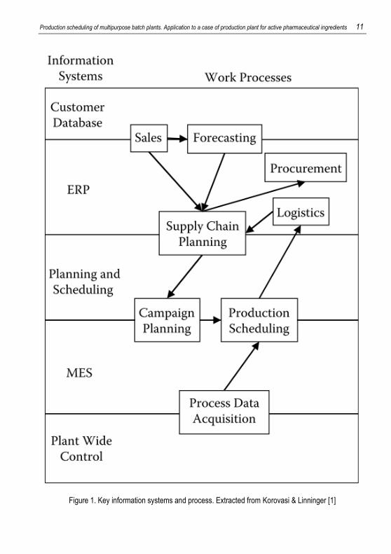
Planning and scheduling fit between the enterprise resource planning (ERP) and
manufacturing execution systems (MES). Figure 1 shows the key information systems that
relate to planning and scheduling. As can be seen, there’s a loop of information between
supply-chain planning, campaign planning and production scheduling. So in order to use all the
available information, a computer-integrated manufacturing (CIM) system must be used. The
CIM system integrates the flow of all the manufacturing information into one computer system.
Edgar [2] said that not all the chemical industry has reached this level of integration.
On chemical industry, there’s a large variety of problems, each one with a different
methodology required in order to solve it, but most of those methods have a similar core.
Specific restrictions, variables and parameters will be used in order to represent all the special
characteristics a problem can have.
Production scheduling of multipurpose batch plants. Application to a case of production plant for active pharmaceutical ingredients 11
Figure 1. Key information systems and process. Extracted from Korovasi & Linninger [1]
12 Rosa Serrat, Bernat
1. OBJECTIVES
In this work, our main objectives are, in one hand, the analysis of the different mathematical
models developed to find the optimal production scheduling in order to give selection criteria
depending on specific problem, and, in the other hand, to use selected models on a real-world
case of a multipurpose plant in order to show the magnitude of the problem.
In order to elaborate the analysis, a bibliographical research will be done, focusing on those
models that could be applied on our problem. Our approach is to explain how these models
work, and how they represent the real-life problems. So, first we will elaborate a classification of
the discussed models, then the models will be described and at last models will be compared,
with a brief explanation on which problems can be used for and why.
To show the magnitude of scheduling problems, we will use the real-world case as an
example. First, we will explain the processes of the plant, and then the scheduling problem with
all its variables. Then we will show two different ways to solve it, one more complex than the
other as it has a higher detail level. On the simpler way, a more detailed analysis will be done;
showing how large is the problem.
Last, we will show our results of real-world case scheduling, obtained after solving the
problem using Wolfram Mathematica, and compare them with non-optimal solutions, with the
idea of showing why optimal solutions are required.
2. OPTIMIZATION MODELS
Mathematical programming has been used for many years to plan and schedule.
Optimization models are based on deterministic data. They determine a set of decision
variables that represent the decisions that must be made, such as start time or allocation of
tasks on units. Together with parameters (constants that define the process, such as processing
time), constraints are generated that specify the restrictions on and interactions between the
decision variables. A feasible solution is any solution that satisfies all the constraints. In order to
determine the optimal solution, an objective function that quantifies the consequences of the
decision variables is needed.
Production scheduling of multipurpose batch plants. Application to a case of production plant for active pharmaceutical ingredients 13
Because the decision variables involve sequencing in addition to resource and equipment
allocation, binary and integer variables are required. Most mathematical models are based on
mixed integer lineal programming (MILP) or mixed integer non-linear programming (MINLP).
Solving as MILP is preferred over a MINLP because of the robustness of the available solvers
and the generally quicker solution times for the problems.
2.1 CLASSIFICATION OF OPTIMIZATION MODELS
Four main aspects are considered in order to elaborate a classification of the models: time
representation, material balances, event representation and objective function.
2.1.1 Time representation
Depending on whether the events of the schedule can only take place at some predefined
time points or can occur at any moment during the time horizon of interest, optimization
approaches can be classified into discrete and continuous time formulations.
Discrete time models
Discrete time models divide the scheduling horizon into a finite number of time intervals with
predefined duration and allow the events such as the beginning or ending of tasks to happen
only at the boundaries of these time periods. Discrete time models have a simpler structure and
are easier to solve, as its constraints are monitored only at those known time points, but the size
of the mathematical model as well as its computational efficiency depend on the number of time
intervals postulated, which is defined as a function of the problem data and the desired
accuracy of the solution. Also sub-optimal or even infeasible schedules may be generated
because of the reduction of the domain of timing decisions. Despite being simplified versions,
discrete time models can be convenient for a wide variety of industrial applications, especially in
those cases where a reasonable number of intervals is sufficient to obtain the desired problem
representation.
Continuous time models
In these formulations, timing decisions are represented as continuous variables defining the
exact times at which the events take place. On this models, less variables are needed and more
flexible solutions can be generated, but because of the modeling of variable processing times,
14 Rosa Serrat, Bernat
resource and inventory limitations usually needs the definition of more complicated constraints,
which increase the model complexity.
2.1.2 Material balances
One thing we need to know is the batching of the process, which is the optimization of the
number of batches and the size of each one. It can be either integrated in the optimization
model or not. If it’s integrated, usually implies large model sizes, so its scheduling horizons
should be shorter. These models employ state-task network (STN) or resource-task network
(RTN) concept to represent the problem. STN-based models represent the problem assuming
that processing tasks produce and consume states (materials). The RTN-based formulations
employ a uniform treatment and representation framework for all available resources through
the idea that processing and storage tasks consume and release resources at their beginning
and ending times, respectively.
For detailed production scheduling two stages are used. First batching converts the primary
requirements of products into individual batches aiming at optimizing some criterion. Then those
batches are allocated using the available manufacturing resource. This method can deal with
larger problems, especially when there are quite intermediates or final products.
2.1.3 Event representation
Scheduling models are based on different concepts that arrange the events of the schedule
over time, so the maximum capacity of the shared resources is never exceed. There are five
cases, but precedence representations include three different modes that are really similar
between them:
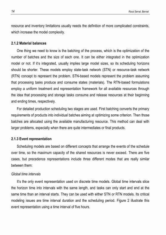
Global time intervals
It’s the only event representation used on discrete time models. Global time intervals slice
the horizon time into intervals with the same length, and tasks can only start and end at the
same time than an interval starts. They can be used with either STN or RTN models. Its critical
modeling issues are time interval duration and the scheduling period. Figure 2 illustrate this
event representation using a time interval of five hours.
Production scheduling of multipurpose batch plants. Application to a case of production plant for active pharmaceutical ingredients 15
Figure 2. Global time intervals representation
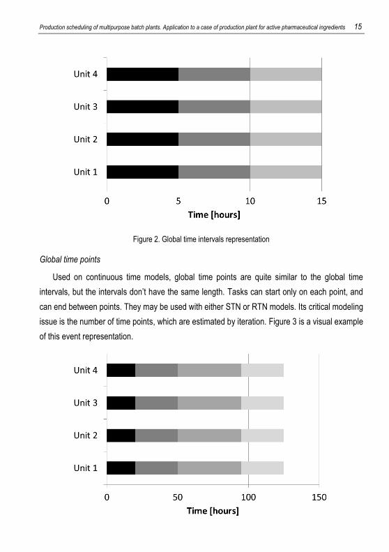
Global time points
Used on continuous time models, global time points are quite similar to the global time
intervals, but the intervals don’t have the same length. Tasks can start only on each point, and
can end between points. They may be used with either STN or RTN models. Its critical modeling
issue is the number of time points, which are estimated by iteration. Figure 3 is a visual example
of this event representation.
16 Rosa Serrat, Bernat
Figure 3. Global time points representation
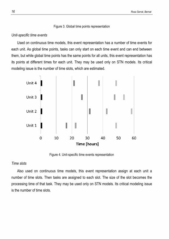
Unit-specific time events
Used on continuous time models, this event representation has a number of time events for
each unit. As global time points, tasks can only start on each time event and can end between
them, but while global time points has the same points for all units, this event representation has
its points at different times for each unit. They may be used only on STN models. Its critical
modeling issue is the number of time slots, which are estimated.
Figure 4. Unit-specific time events representation
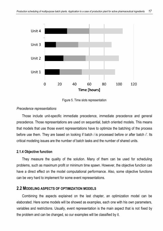
Time slots
Also used on continuous time models, this event representation assign at each unit a
number of time slots. Then tasks are assigned to each slot. The size of the slot becomes the
processing time of that task. They may be used only on STN models. Its critical modeling issue
is the number of time slots.
Production scheduling of multipurpose batch plants. Application to a case of production plant for active pharmaceutical ingredients 17
Figure 5. Time slots representation
Precedence representations
Those include unit-specific immediate precedence, immediate precedence and general
precedence. Those representations are used on sequential, batch oriented models. This means
that models that use those event representations have to optimize the batching of the process
before use them. They are based on looking if batch i is processed before or after batch i’. Its
critical modeling issues are the number of batch tasks and the number of shared units.
2.1.4 Objective function
They measure the quality of the solution. Many of them can be used for scheduling
problems, such as maximum profit or minimum time spawn. However, the objective function can
have a direct effect on the model computational performance. Also, some objective functions
can be very hard to implement for some event representations.
2.2 MODELING ASPECTS OF OPTIMIZATION MODELS
Combining the aspects explained on the last chapter, an optimization model can be
elaborated. Here some models will be showed as examples, each one with his own parameters,
variables and restrictions. Usually, event representation is the main aspect that is not fixed by
the problem and can be changed, so our examples will be classified by it.
18 Rosa Serrat, Bernat
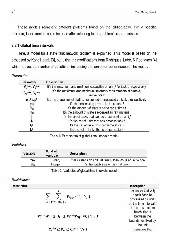
Those models represent different problems found on the bibliography. For a specific
problem, those models could be used after adapting to the problem’s characteristics.
2.2.1 Global time intervals
Here, a model for a state task network problem is explained. This model is based on the
proposed by Kondili et al. [3], but using the modifications from Rodrigues, Latre, & Rodrigues [4]
which reduce the number of equations, increasing the computer performance of the model.
Parameters
Parameter Description
Vijmax, Vij
min It’s the maximum and minimum capacities on unit j for task i, respectively
Csmax, Cs
min It’s the maximum and minimum inventory requirements of state s, respectively
ρisc, ρis
p It’s the proportion of state s consumed or produced on task i, respectively ptij It’s the processing time of task i on unit j Dst It’s the amount of state s delivered at time t Пst It’s the amount of state s received as raw material Ij It’s the set of tasks that can be processed on unit j Ji It’s the set of units that can process task i Isc It’s the set of tasks that consume state s Isp It’s the set of tasks that produce state s
Table 1. Parameters of global time intervals model
Variables
Variable Kind of variable
Description
Wijt Binary If task i starts on unit j at time t, then Wijt is equal to one Bijt Integer It’s the batch size of task i at time t.
Table 2. Variables of global time intervals model
Restrictions
Restriction Description
∑ ∑
It ensures that only a task i can be
processed on unit j on the time interval t
It ensures that the batch size is between the
boundaries fixed by the unit
It ensures that
Production scheduling of multipurpose batch plants. Application to a case of production plant for active pharmaceutical ingredients 19
inventory requirements of
state s are always accomplished
∑ ∑
∑ ∑
∏
Represents the material balance of
state s on time t
Table 3. Restrictions of global time intervals model
As it’s said, global time intervals is the only model used on discrete time. It is a simplified
model, and it’s a good option when a small amount of time intervals are required. This means
that processing times have a maximum common denominator high enough to seize the horizon
time on a few time intervals. They have a problem with changeover time, as usually those are
small compared with processing times and lean to smaller maximum common denominators, so
on process where those are critical (because there are a lot of changeovers, or they got a cost
assigned) this model is not desirable.
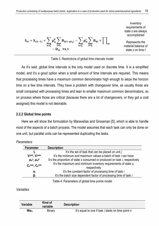
2.2.2 Global time points
Here we will show the formulation by Maravelias and Grossman [5], which is able to handle
most of the aspects of a batch process. The model assumes that each task can only be done on
one unit, but parallel units can be represented duplicating the tasks.
Parameters
Parameter Description
Ij It’s the set of task that can be placed on unit j Vi
min, Vimax It’s the minimum and maximum values a batch of task i can have
ρisc, ρis
p It’s the proportion of state s consumed or produced on task i, respectively
Csmax, Cs
min It’s the maximum and minimum inventory requirements of state s,
respectively αi It’s the constant factor of processing time of task i βi It’s the batch size dependent factor of processing time of task i
Table 4. Parameters of global time points model
Variables
Variable Kind of variable
Description
Wsin Binary It’s equal to one if task i starts on time point n
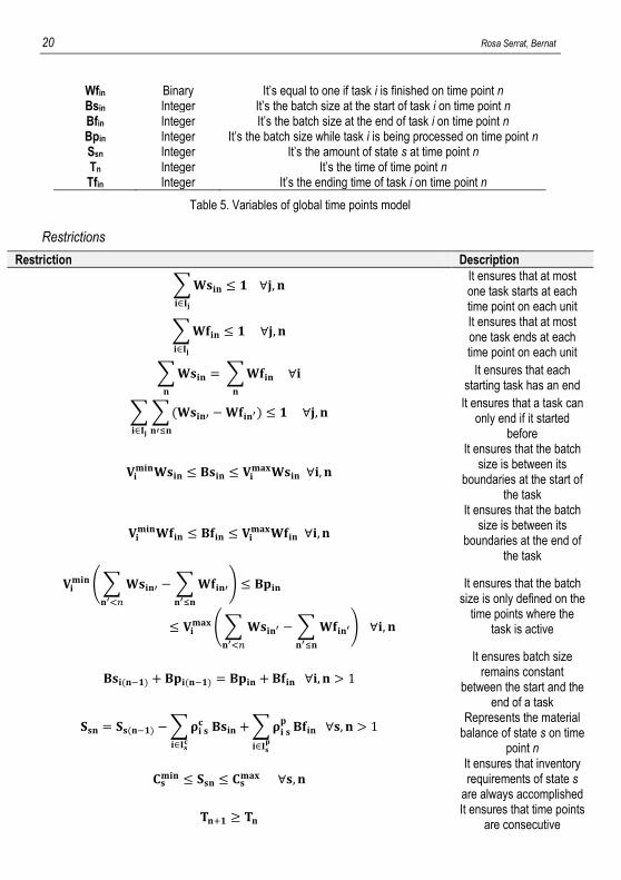
20 Rosa Serrat, Bernat
Wfin Binary It’s equal to one if task i is finished on time point n Bsin Integer It’s the batch size at the start of task i on time point n Bfin Integer It’s the batch size at the end of task i on time point n Bpin Integer It’s the batch size while task i is being processed on time point n Ssn Integer It’s the amount of state s at time point n Tn Integer It’s the time of time point n Tfin Integer It’s the ending time of task i on time point n
Table 5. Variables of global time points model
Restrictions
Restriction Description
∑
It ensures that at most one task starts at each time point on each unit
∑
It ensures that at most one task ends at each time point on each unit
∑
∑
It ensures that each starting task has an end
∑ ∑
It ensures that a task can
only end if it started before
It ensures that the batch size is between its
boundaries at the start of the task
It ensures that the batch size is between its
boundaries at the end of the task
(∑
∑
)
(∑
∑
)
It ensures that the batch size is only defined on the
time points where the task is active
It ensures batch size remains constant
between the start and the end of a task
∑
∑
Represents the material
balance of state s on time point n
It ensures that inventory requirements of state s
are always accomplished
It ensures that time points
are consecutive
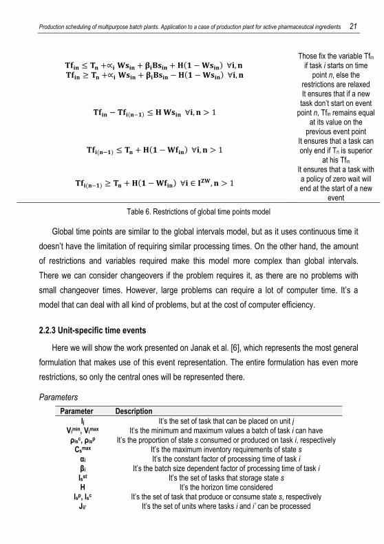
Production scheduling of multipurpose batch plants. Application to a case of production plant for active pharmaceutical ingredients 21
Those fix the variable Tfin if task i starts on time
point n, else the restrictions are relaxed
It ensures that if a new task don’t start on event
point n, Tfin remains equal at its value on the
previous event point
It ensures that a task can only end if Tn is superior
at his Tfin
It ensures that a task with a policy of zero wait will end at the start of a new
event
Table 6. Restrictions of global time points model
Global time points are similar to the global intervals model, but as it uses continuous time it
doesn’t have the limitation of requiring similar processing times. On the other hand, the amount
of restrictions and variables required make this model more complex than global intervals.
There we can consider changeovers if the problem requires it, as there are no problems with
small changeover times. However, large problems can require a lot of computer time. It’s a
model that can deal with all kind of problems, but at the cost of computer efficiency.
2.2.3 Unit-specific time events
Here we will show the work presented on Janak et al. [6], which represents the most general
formulation that makes use of this event representation. The entire formulation has even more
restrictions, so only the central ones will be represented there.
Parameters
Parameter Description
Ij It’s the set of task that can be placed on unit j Vi
min, Vimax It’s the minimum and maximum values a batch of task i can have
ρisc, ρis
p It’s the proportion of state s consumed or produced on task i, respectively Cs
max It’s the maximum inventory requirements of state s αi It’s the constant factor of processing time of task i βi It’s the batch size dependent factor of processing time of task i Isst It’s the set of tasks that storage state s H It’s the horizon time considered
Isp, Isc It’s the set of task that produce or consume state s, respectively Jii’ It’s the set of units where tasks i and i’ can be processed
22 Rosa Serrat, Bernat
Ji It’s the set of units where task i can be processed Szw it’s the set of states where a zero wait policy is applied
Table 7. Parameters of unit-specific time events model
Variables
Variable Kind of variable
Description
Win Binary It equals to one when task i is active on event point n Wsin Binary It equals to one when task i begins on event point n Wfin Binary It equals to one when task i ends on event point n Bin Integer It’s the batch size of an active task i at event point n Bsin Integer It’s the batch size of a starting task i at event point n Bfin Integer It’s the batch size of an ending task i at event point n
Bistn Integer It’s the batch size of storage task i at event point n Ssn Integer It’s the amount of state s at event point n Tsin Integer It’s the starting time of task i at event point n Tfin Integer It’s the ending time of task i at event point n
Table 8. Variables of unit-specific time events model
Restrictions
Restriction Description
∑
It ensures that at most one task starts at each time point on
each unit
∑
∑
It defines when a task is active
∑
∑
It ensures that
every starting task has an end
∑
∑
It ensures that a task can only start
if all previous starting tasks have ended
∑
∑
It ensures that a task can only end if it started on a previous event point and hasn’t
ended before event point n
It ensures that batch size is between its
Production scheduling of multipurpose batch plants. Application to a case of production plant for active pharmaceutical ingredients 23
boundaries
( )
( )
Those force the batch size to
remain constant as long as the
task is active, as it can go through multiple event
points
This set of restrictions force the batch size at the start of task i to be equal at the
batch size of active task i, only if task i is active,
else those restrictions
become redundant
This set of restrictions force the batch size at the end of task i
to be equal at the batch size of
active task i, only if task i is active,
else those restrictions
become redundant
It ensures that maximum storage
is never surpassed
∑
∑
∑
∑
Represents the material balance
of state s on event point n
Those ensures that if task i is not active on event point n, then its
processing time is equal to zero
( ) If task i is active
24 Rosa Serrat, Bernat
on event point n-1 and doesn’t end
there, this restriction force the starting time of event n to be
equal to the ending time at n-
1. Else, this restriction is
relaxed
( ∑
)
( ∑
)
Those restrictions define the ending
time of a task i starting at event
point n and ending at a later event point n’, so
ending time of event point n’ is equal to starting time of n plus the processing time of
i
It ensures that
tasks are sequential
( )
It ensures that task i can only start after its
correspondent changeover, if it’s
consecutive to task i’
( )
It ensures that if a task i’ produces state s and task i consumes that s, then task i would
be processed right after i’
( )
It ensures a zero wait police on a
state s
Table 9. Restrictions of unit-specific time events model
Similar to the global time points, this model is more computer efficient on problems where
only few units are used or the processing times of the problem’s tasks are really different
Production scheduling of multipurpose batch plants. Application to a case of production plant for active pharmaceutical ingredients 25
between themselves. On this cases, it can solve the same problem with less events than the
global time points requires, meaning that less variables and restrictions would be required and
thus getting and answer faster. However, it’s not as flexible as global time points and there are
cases where it would be less computer efficiently, as the extra restrictions and variables of the
model won’t be compensated by the fewer events.
2.2.4 Time slots
Here we will show the original model of time slots developed by Pinto and Grossman [7],
assuming a multistage sequential scheduling problem with parallel units.
Parameters
Parameter Description
Li It’s the set of processing stages of batch i Kj It’s the set of slots of unit j Jil It’s the set of units where processing stages l of batch i can be processed pij It’s the processing task of batch i on unit j
Suij It’s the setup time of batch i on unit j M A large integer number
Table 10. Parameters of time slots model
Variables
Variable Kind of variable
Description
Wijkl Binary If processing stage l of batch i starts on unit j at slot k, then it equals to
one Tsil Integer It’s the starting time of processing stage l of batch i Tsjk Integer It’s the starting time of slot k on unit j Tfil Integer It’s the ending time of processing stage l of batch i Tfjk Integer It’s the ending time of slot k on unit j
Table 11. Variables of time slots model
Restrictions
Restriction Description
∑ ∑
It ensures that every processing task of a batch i is assigned to a
slot
∑∑
It ensures that at most each slot has at most one processing task
assigned
( )
( )
Those restrictions force the starting time of a slot on unit j to
26 Rosa Serrat, Bernat
be equal to the starting time of processing task from batch i, if
it’s assigned to that slot.
∑∑
∑ ∑
( )
Those restrictions force the ending times of the slot and the
processing task to coincide when the task is assigned at that slot.
It enforces that no overlap
between time slots happens
It enforces that processing tasks are sequential. For a zero wait police, this restriction must be
equality.
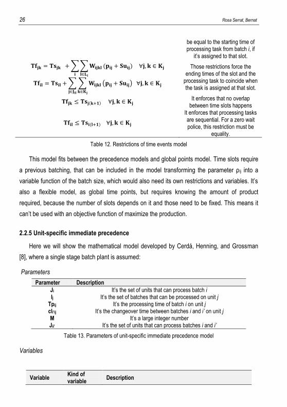
Table 12. Restrictions of time events model
This model fits between the precedence models and global points model. Time slots require
a previous batching, that can be included in the model transforming the parameter ρ ij into a
variable function of the batch size, which would also need its own restrictions and variables. It’s
also a flexible model, as global time points, but requires knowing the amount of product
required, because the number of slots depends on it and those need to be fixed. This means it
can’t be used with an objective function of maximize the production.
2.2.5 Unit-specific immediate precedence
Here we will show the mathematical model developed by Cerdá, Henning, and Grossman
[8], where a single stage batch plant is assumed:
Parameters
Parameter Description
Ji It’s the set of units that can process batch i Ij It’s the set of batches that can be processed on unit j
Tpij It’s the processing time of batch i on unit j cli’ij It’s the changeover time between batches i and i’ on unit j M It’s a large integer number Jii’ It’s the set of units that can process batches i and i’
Table 13. Parameters of unit-specific immediate precedence model
Variables
Variable Kind of variable
Description
Production scheduling of multipurpose batch plants. Application to a case of production plant for active pharmaceutical ingredients 27
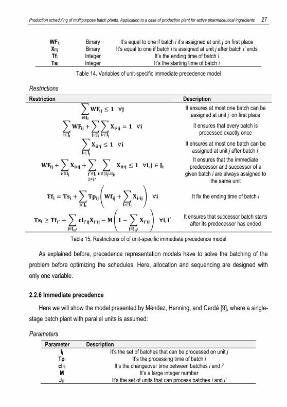
WFij Binary It’s equal to one if batch i it’s assigned at unit j on first place Xi’ij Binary It’s equal to one if batch i is assigned at unit j after batch i’ ends Tfi Integer It’s the ending time of batch i Tsi Integer It’s the starting time of batch i
Table 14. Variables of unit-specific immediate precedence model
Restrictions
Restriction Description
∑
It ensures at most one batch can be assigned at unit j on first place
∑
∑∑
It ensures that every batch is processed exactly once
∑
It ensures at most one batch can be assigned at unit j after batch i’
∑
∑ ∑
It ensures that the immediate
predecessor and successor of a given batch i are always assigned to
the same unit
∑ ( ∑
)
It fix the ending time of batch i
∑
( ∑
) It ensures that successor batch starts
after its predecessor has ended
Table 15. Restrictions of of unit-specific immediate precedence model
As explained before, precedence representation models have to solve the batching of the
problem before optimizing the schedules. Here, allocation and sequencing are designed with
only one variable.
2.2.6 Immediate precedence
Here we will show the model presented by Méndez, Henning, and Cerdá [9], where a single-
stage batch plant with parallel units is assumed:
Parameters
Parameter Description
Ij It’s the set of batches that can be processed on unit j Tpi It’s the processing time of batch i cli’i It’s the changeover time between batches i and i’ M It’s a large integer number Jii’ It’s the set of units that can process batches i and i’
28 Rosa Serrat, Bernat
Table 16. Parameters of immediate precedence model
Variables
Variable Kind of variable
Description
WFij Binary It’s equal to one if batch i it’s assigned at unit j on first place Wij Binary It’s equal to one if batch i is assigned at unit j but not on first place Xi’i Binary It’s equal to one if batch i’ it’s the immediate predecessor of i Tfi Integer It’s the ending time of batch i Tsi Integer It’s the starting time of batch i
Table 17. Variables of immediate precedence model
Restrictions
Restriction Description
∑
It ensures that at most one batch would be processed first on unit j
∑
∑
It ensures that all batches are allocated on a unit
Those ensures that a batch i predeceased by i’ would be allocated on the same unit j
∑
∑
It ensures that a batch would be processed only once
∑
It ensures each batch would have at most one predecessor
∑
It fixes the ending time of batch i
∑( )
It prevents batch overlapping
Table 18. Restrictions of immediate precedence model
In contrast with the previous model, here allocation and sequencing decisions are divided
into two different sets of binary variables.
2.2.7 General precedence
Here a model developed by Méndez, Henning and Cerdá [10] is showed, assuming a
multistage sequential scheduling problem with multiple parallel units:
Production scheduling of multipurpose batch plants. Application to a case of production plant for active pharmaceutical ingredients 29
Parameters
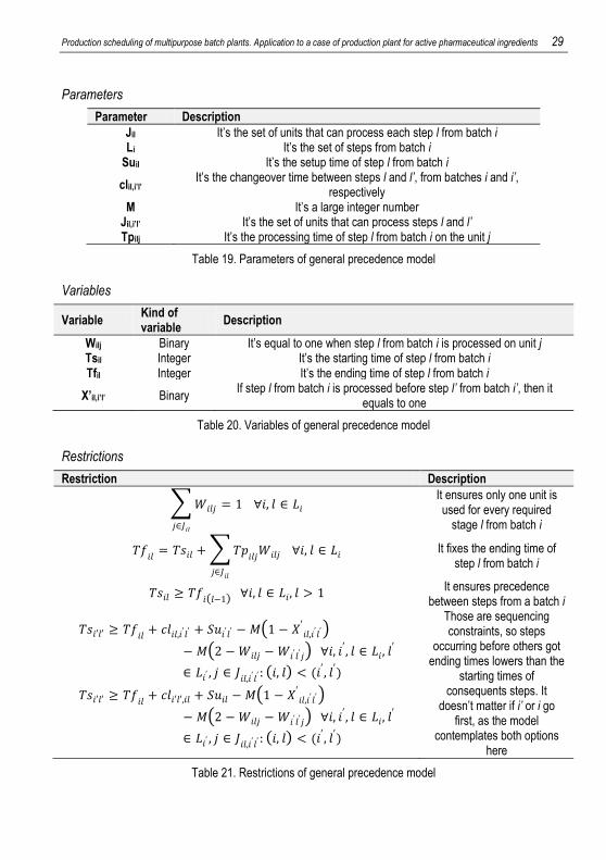
Parameter Description
Jil It’s the set of units that can process each step l from batch i Li It’s the set of steps from batch i
Suil It’s the setup time of step l from batch i
clil,i’l’ It’s the changeover time between steps l and l’, from batches i and i’,
respectively M It’s a large integer number
Jil,i’l’ It’s the set of units that can process steps l and l’ Tpilj It’s the processing time of step l from batch i on the unit j
Table 19. Parameters of general precedence model
Variables
Variable Kind of variable
Description
Wilj Binary It’s equal to one when step l from batch i is processed on unit j Tsil Integer It’s the starting time of step l from batch i Tfil Integer It’s the ending time of step l from batch i
X’il,i’l’ Binary If step l from batch i is processed before step l’ from batch i’, then it
equals to one
Table 20. Variables of general precedence model
Restrictions
Restriction Description
∑
It ensures only one unit is used for every required
stage l from batch i
∑
It fixes the ending time of step l from batch i
It ensures precedence between steps from a batch i
(
)
( )
(
)
( )
Those are sequencing constraints, so steps
occurring before others got ending times lowers than the
starting times of consequents steps. It
doesn’t matter if i’ or i go first, as the model
contemplates both options here
Table 21. Restrictions of general precedence model
30 Rosa Serrat, Bernat
This model not only looks at the immediate precedence, but considers all the previous
batches processed before.
3. THE REAL CASE
3.1 THE PROCESS
The real-case is a multipurpose batch plant processing both rifaximin and fosfomycin,
alongside other products that take place on another zone of the plant. Our equipment consists
of four identical reactors (R1, R2, R3, R4), two filters (F5, F6), two centrifuges (C7, C8), four
rotatory dryers (D11, D12, D13, D14), an ionic exchange column (B9) used explicitly on
fosfomycin production with his regeneration equipment (B10), two sieves (S15, S16) and a set
of pipes, bombs and other auxiliary equipment. We won’t take into account limitations such as
number of employers (which could be a problem when multiple tasks begging at the same time)
or auxiliary resources limitation.
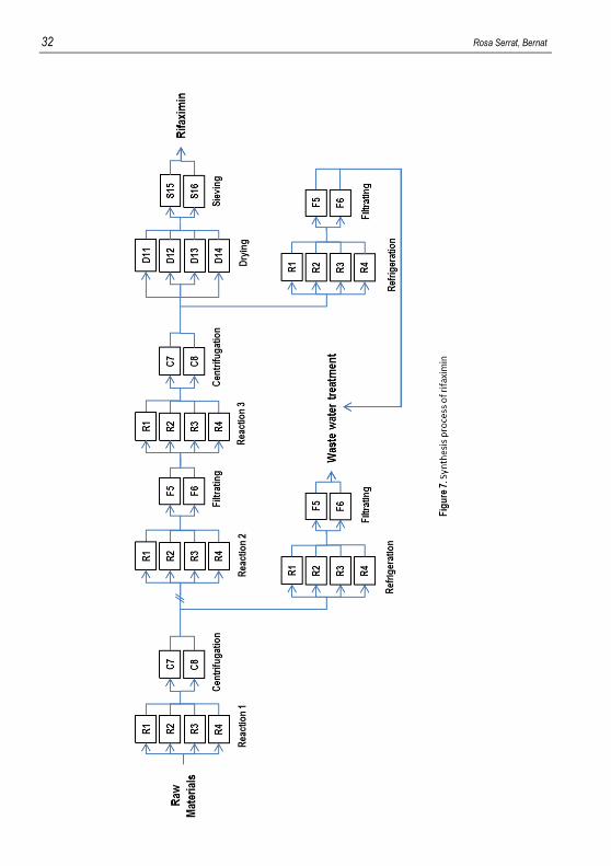
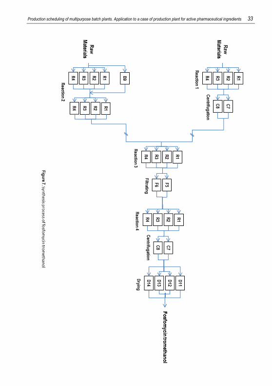
Rifaximin is an API (Active Pharmaceutical Ingredient), an antibiotic used for diarrhea and to
prevent the effects of a hepatic encephalopathy. On this plant is produced on a two steps
process.
Fosfomycin tromethanol is an API, a broad-spectrum antibiotic used on urinary tract
infections. On this plant is produced in a three steps process.
Each step has an amount of tasks, which are formed from a set of subtasks. For example,
on the process of rifaximin, its first step (producing technical rifaximin) is formed from the next
tasks: reaction 1 (which includes as subtasks charging the reactor with the raw materials, the
reaction, the precipitation of the products, the discharge of the reactor and its cleaning),
centrifugation, refrigeration of the mother liquors, filtrating and sending to waste water
treatment.
Figure 6 and Figure 7 show the two processes with each task and which units can do those.
As it can be seen, most tasks can be processed on multiple units.

Production scheduling of multipurpose batch plants. Application to a case of production plant for active pharmaceutical ingredients 31
A manual approach to the problem would take a large amount of time. With a rough
estimation, we have about nine hundred billions of possible schedules in order to elaborate one
batch of each product, and it has an exponential ratio with the number of batches, so for two
batches of each product we would talk about 7·1020 possible schedules. While not all are viable,
and only a few would result optimal, that’s still a huge number of possibilities, and we are
looking only at the tasks, not the subtasks, which would increase even more the number of non-
viable or non-optimal solutions. Moreover, there we are not considering things as batching,
which affect at the process time and the number of batches.
Also, the process has some restrictions. Most tasks must commit right after another and
some subtasks must be processed at the same time (for example, the discharge of a reactor,
the filtration of the discharged product and the charge of the reactor where the filtrated product
goes are active at the same time). Moreover, subtasks from a task must be processed on the
same unit. Usually a horizon time will be fixed, so our products should be ready before that time.
Obviously, a unit can only process one task each time, and the process can only be stopped at
the end of each step.
As it can be seen, a manual approach is not viable at all on this problem. In order to found
an optimal solution, a mathematical model must be done which contains all the characteristics
of the problem.
32 Rosa Serrat, Bernat
Production scheduling of multipurpose batch plants. Application to a case of production plant for active pharmaceutical ingredients 33
34 Rosa Serrat, Bernat
3.2 MODELING ASPECTS OF THE PROCESS
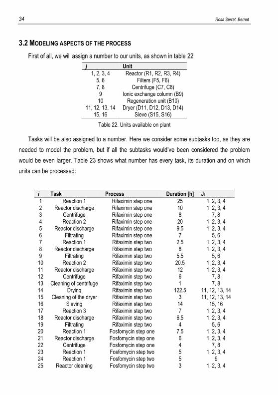
First of all, we will assign a number to our units, as shown in table 22
j Unit
1, 2, 3, 4 Reactor (R1, R2, R3, R4) 5, 6 Filters (F5, F6) 7, 8 Centrifuge (C7, C8)
9 Ionic exchange column (B9) 10 Regeneration unit (B10)
11, 12, 13, 14 Dryer (D11, D12, D13, D14) 15, 16 Sieve (S15, S16)
Table 22. Units available on plant
Tasks will be also assigned to a number. Here we consider some subtasks too, as they are
needed to model the problem, but if all the subtasks would’ve been considered the problem
would be even larger. Table 23 shows what number has every task, its duration and on which
units can be processed:
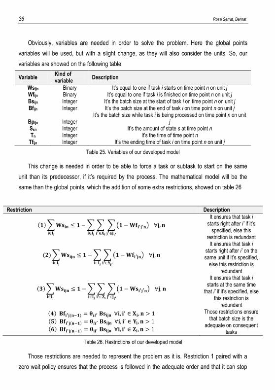
i Task Process Duration [h] Ji
1 Reaction 1 Rifaximin step one 25 1, 2, 3, 4 2 Reactor discharge Rifaximin step one 10 1, 2, 3, 4 3 Centrifuge Rifaximin step one 8 7, 8 4 Reaction 2 Rifaximin step one 20 1, 2, 3, 4 5 Reactor discharge Rifaximin step one 9.5 1, 2, 3, 4 6 Filtrating Rifaximin step one 7 5, 6 7 Reaction 1 Rifaximin step two 2.5 1, 2, 3, 4 8 Reactor discharge Rifaximin step two 8 1, 2, 3, 4 9 Filtrating Rifaximin step two 5.5 5, 6 10 Reaction 2 Rifaximin step two 20.5 1, 2, 3, 4 11 Reactor discharge Rifaximin step two 12 1, 2, 3, 4 12 Centrifuge Rifaximin step two 6 7, 8 13 Cleaning of centrifuge Rifaximin step two 1 7, 8 14 Drying Rifaximin step two 122.5 11, 12, 13, 14 15 Cleaning of the dryer Rifaximin step two 3 11, 12, 13, 14 16 Sieving Rifaximin step two 14 15, 16 17 Reaction 3 Rifaximin step two 7 1, 2, 3, 4 18 Reactor discharge Rifaximin step two 6.5 1, 2, 3, 4 19 Filtrating Rifaximin step two 4 5, 6 20 Reaction 1 Fosfomycin step one 7.5 1, 2, 3, 4 21 Reactor discharge Fosfomycin step one 6 1, 2, 3, 4 22 Centrifuge Fosfomycin step one 4 7, 8 23 Reaction 1 Fosfomycin step two 5 1, 2, 3, 4 24 Reaction 1 Fosfomycin step two 5 9 25 Reactor cleaning Fosfomycin step two 3 1, 2, 3, 4
Production scheduling of multipurpose batch plants. Application to a case of production plant for active pharmaceutical ingredients 35
26 Reaction 2 Fosfomycin step two 8 1, 2, 3, 4 27 Reaction 1 Fosfomycin step three 3.5 1, 2, 3, 4 28 Reactor discharge Fosfomycin step three 5.5 1, 2, 3, 4 29 Filtrating Fosfomycin step three 2.5 5, 6 30 Reaction 2 Fosfomycin step three 20 1, 2, 3, 4 31 Reactor discharge Fosfomycin step three 7 1, 2, 3, 4 32 Centrifuge Fosfomycin step three 4 7, 8 33 Centrifuge cleaning Fosfomycin step three 1 7, 8 34 Drying Fosfomycin step three 6 11, 12, 13, 14 35 Regeneration Fosfomycin regeneration 21 10 36 Regeneration Fosfomycin regeneration 21 9
Table 23. Tasks processed on our plant
Now that we have both units and tasks, next step is the time. Our base model will be the
global points model, as precedence models and unit-based event points don’t let us start
subtasks at the same time, global interval can’t be used on continuous time (and we got such a
disparity on task’s ending times that makes discrete time a non-desirable option) and slot-based
models won’t let us use as objective function the maximum production on a given horizon time,
which is the easiest objective function to implant. Also, global point model can be adapted to our
problem with only a few minor changes.
So, our set of units is J, I stands for the set of tasks and N would be our global points.
Parameters we will need to concrete our problem are listed on table 24:
Parameter Description
Ij It’s the set of task that can be placed on unit j Vi
min, Vimax It’s the minimum and maximum values a batch of task i can have
ρisc, ρis
p It’s the proportion of state s consumed or produced on task i, respectively
Csmax, Cs
min It’s the maximum and minimum inventory requirements of state s,
respectively αi It’s the constant factor of processing time of task i Xi It’s the set of tasks that must be processed right before i. βi It’s the batch size dependent factor of processing time of task i Zi It’s the set of tasks that must start at the same time than i θii’ It’s the proportion between batch size on task i and task i’
Table 24. Parameters of our developed model
Those are the usual parameters on global points, except for the last four, which are
exclusive of this problem.
36 Rosa Serrat, Bernat
Obviously, variables are needed in order to solve the problem. Here the global points
variables will be used, but with a slight change, as they will also consider the units. So, our
variables are showed on the following table:
Variable Kind of variable
Description
Wsijn Binary It’s equal to one if task i starts on time point n on unit j Wfijn Binary It’s equal to one if task i is finished on time point n on unit j Bsijn Integer It’s the batch size at the start of task i on time point n on unit j Bfijn Integer It’s the batch size at the end of task i on time point n on unit j
Bpijn Integer It’s the batch size while task i is being processed on time point n on unit
j Ssn Integer It’s the amount of state s at time point n Tn Integer It’s the time of time point n
Tfijn Integer It’s the ending time of task i on time point n on unit j
Table 25. Variables of our developed model
This change is needed in order to be able to force a task or subtask to start on the same
unit than its predecessor, if it’s required by the process. The mathematical model will be the
same than the global points, which the addition of some extra restrictions, showed on table 26
Restriction Description
∑
∑ ∑ ∑( )
It ensures that task i starts right after i’ if it’s
specified, else this restriction is redundant
∑
∑ ∑ ( )
It ensures that task i starts right after i’ on the same unit if it’s specified,
else this restriction is redundant
∑
∑ ∑ ∑( )
It ensures that task i starts at the same time
that i’ if it’s specified, else this restriction is
redundant
Those restrictions ensure that batch size is the
adequate on consequent tasks
Table 26. Restrictions of our developed model
Those restrictions are needed to represent the problem as it is. Restriction 1 paired with a
zero wait policy ensures that the process is followed in the adequate order and that it can stop

Production scheduling of multipurpose batch plants. Application to a case of production plant for active pharmaceutical ingredients 37
only at the end of a step. Restriction 2 is needed so consequent subtasks from a single task
happen on the same unit. Restriction 3 is needed because, as explained before, there are some
subtasks that must start at the same time, like the charge of a reactor with the discharge of the
previous reactor. Restrictions 4, 5 and 6 are there to ensure that the global mass balance of the
process remains constant, and no changes occur between tasks.
When trying to solve this problem with this model, we find that is such a large problem that
our computer is not prepared to solve it. It’s both a hardware and software problem, as neither
our computer is prepared for intensive CPU usage, and our software, Wolfram Mathematica, is
a generic software that is not specialized on this kind of problems. In order to solve the problem
with our tools, a simplified version of it is considered.
3.2.2 Simplified Model
Here, the main change is the number of tasks and the number of units. We will consider
only the steps of the processes and two groups of units, each one including two reactors, a
centrifuge, and a filter. The ionic-exchange column, its regeneration system, the dryers and the
sieves and the tasks that happen are also considered, but not all in an explicit way.
Another thing that will be simplified is the batch size, which will be fixed. This allows us to
take out all the restrictions and variables related to the batch size, and also make the
processing time of each task a constant.
So, on this simplified model, those are our units:
j Unit
1, 2 Basic equipment 3 Regeneration
4, 5, 6, 7 Dryers
Table 27. Simplified units available on our plant
The ionic exchange column will be represented using the resin as a prime material that
would be consumed on the corresponding step and will be produced by the regeneration task.
Also, no more than one batch of resin can be storage, so after each use of the column,
regeneration is required. Sieving time is added at dryer’s time, as with our layout never more
than two sieves will be required at once. This way, fewer variables are required and the model
requires less computer time, at the cost of precision.
38 Rosa Serrat, Bernat
Therefore, those would be our tasks:
i Task Process Duration [h] Ji
1 Rifaximin step one Rifaximin 55 1, 2 2 Rifaximin step two Rifaximin 70 1, 2 3 Rifaximin drying Rifaximin 136.5 4, 5, 6, 7 4 Fosfomicyn step one Fosfomicyn 14 1, 2 5 Fosfomicyn step two Fosfomicyn 13 1, 2 6 Fosfomicyn step three Fosfomicyn 31 1, 2 7 Fosfomicyn drying Fosfomicyn 5 4, 5, 6, 7 8 Regeneration Fosfomicyn 29 3
Table 28. Simplified tasks processed on our plant
We are considering eight tasks instead of thirty-six, so our number of variables decreases
dramatically. Rifaximin’s drying includes the sieving, as stated before.
Even with those simplifications, the problem is still large enough to be needed to solve with
a computer. As a rough estimation, there are sixteen millions of schedules when trying to
produce a batch of each product.
The simplified problem can be easily adapted to other mathematical models, like the unit-
specific time event or time slots, as there are no tasks starting at the same time. Still, if our
objective function is maximum production, time slots can’t be used.
On our next section we will show our results and compare them to non-optimized schedules.
Our program can be found on the annexes.
3.3 RESULTS
With these results, our main objective is to show that an optimization can have a great
impact on a problem. The objective function used here is maximum production. In order to be
able to solve the problem a small horizon time of two weeks has been fixed, so less event points
will be needed.
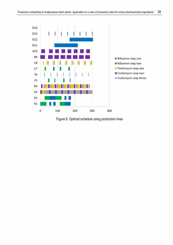
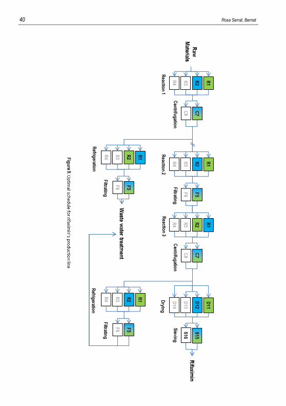
Figure 8 shows the scheduling for our plant if two lines of production are used, one for
rifaximin and the other for fosfomycin tromethanol. The same schedule is showed on fig 9 for
the rifaximin batches, on an easier way to follow it. Grey units are those that belong to the
fosfomycin production line, and therefore can’t be used for rifaximin production. Green units are
those that are used on the first batch of rifaximin and blue units represent those used on the
second batch.
Production scheduling of multipurpose batch plants. Application to a case of production plant for active pharmaceutical ingredients 39
Figure 8. Optimal schedule using production lines
40 Rosa Serrat, Bernat
Production scheduling of multipurpose batch plants. Application to a case of production plant for active pharmaceutical ingredients 41
Schedules from the other solutions can be found on appendix I. Table 29 shows the results
obtained:
Method
Batches of fosfomycin with
none of rifaximin
Batches of fosfomycin with
one batch of rifaximin
Batches of fosfomycin with two batches of
rifaximin
Batches of fosfomycin with three batches of
rifaximin Production lines
without simplification
8 8 8 -
Production lines with
simplification 5 5 - -
Non-optimized model with
simplification 7 6 4 -
Optimized model with
simplification 7 6 5 -
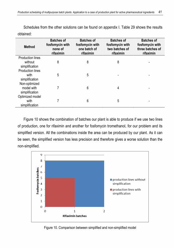
Figure 10 shows the combination of batches our plant is able to produce if we use two lines
of production, one for rifaximin and another for fosfomycin tromethanol, for our problem and its
simplified version. All the combinations inside the area can be produced by our plant. As it can
be seen, the simplified version has less precision and therefore gives a worse solution than the
non-simplified.
Figure 10. Comparison between simplified and non-simplified model
42 Rosa Serrat, Bernat
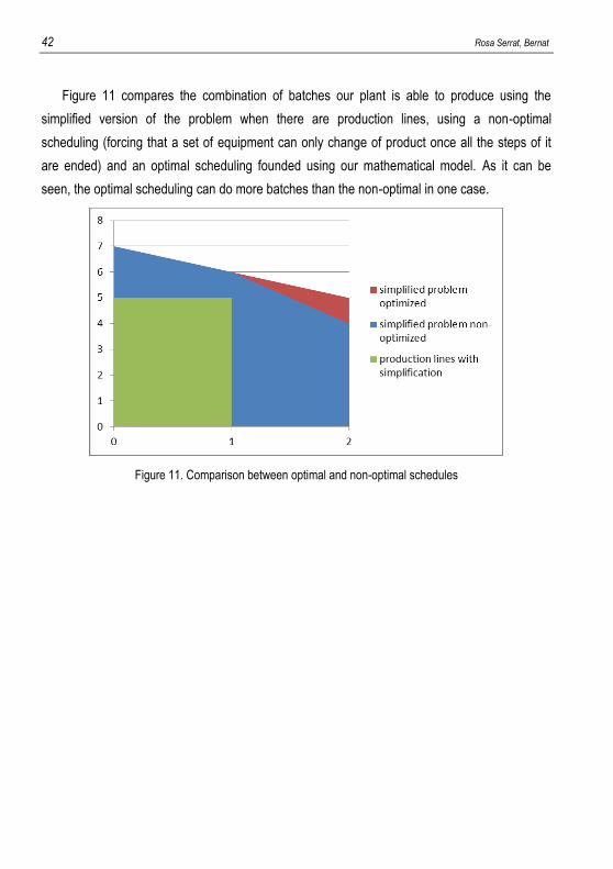
Figure 11 compares the combination of batches our plant is able to produce using the
simplified version of the problem when there are production lines, using a non-optimal
scheduling (forcing that a set of equipment can only change of product once all the steps of it
are ended) and an optimal scheduling founded using our mathematical model. As it can be
seen, the optimal scheduling can do more batches than the non-optimal in one case.
Figure 11. Comparison between optimal and non-optimal schedules
Production scheduling of multipurpose batch plants. Application to a case of production plant for active pharmaceutical ingredients 43
4. CONCLUSIONS
After analyzing the different models found on the bibliography, one of the conclusions of the
work is that each problem requires a specific model for it, so there is no universal model that
can be used always. This lead to generic models that with a few modifications can be used in a
wide amount of problems, but even those generic models can’t be used on all the kinds of
problems. Those generic models differ basically on which kind of event representation use and
how their material balances are represented.
For our real world problem, a model using global time points as its event representation has
been developed. Of all the possible event representations, it is the one that not only can
represent the problem as it is, also does it in a simple way and can be easily adapted to similar
problems, such as a different objective function or a change on the number of units. Discrete
time can’t be used there, as there is a big gap between the times required for each task, so a lot
of time intervals would be needed, making it unviable. The other continuous time event
representations either can’t be adapted to our problem for its special characteristics, like forcing
tasks to start at the same time on different units, or can’t be easily adapted to it, which leads to
a large problem.
The optimization model is still a large problem, so a simplified version of it is developed.
Comparing the schedules between the simplified version and the original problem, assuming
production lines, a remarkable diminution of the capacity of the plant is observed, so we can
assume that the simplification, while necessary for our problem, leads to worse solutions than
the original model. A conclusion we can take from here is that, when elaborating an optimization
model, the simpler it is the better it will work, as those models grow exponentially with the
horizon time. Therefore, a critical part of the scheduling optimization is the selection of the
adequate event representation, mass balance representation, time representation and objective
function.
With the results, it can be seen that the optimized schedule allows to an extra fosfomycin
batch when two batches of rifaximin are produced, compared with a non-optimized schedule.
With a horizon time of two weeks, that’s an important increase, so one conclusion is that the
optimization is valuable. Also, both the optimized and non-optimized schedules are better way
than using production lines, so if there are no problems of cross-product contamination
production lines should be avoided.

44 Rosa Serrat, Bernat
Production scheduling of multipurpose batch plants. Application to a case of production plant for active pharmaceutical ingredients 45
REFERENCES AND NOTES 1. Korovesi, Ekaterini; Linninger, Andreas A. Batch Processes, 1st ed.; Taylor & Francis Group, LLC. 2. Edgar, T.F (2000)., Process information: achieving a unified view, Chem. Eng. Prog., 96, 51–57. 3. Kondili, E., Pantelides, C. C., & Sargent, W. H. (1993). A general algorithm for short-term scheduling
of batch operations-I. MILP formulation. Computers and Chemical Engineering, 2, 211–227. 4. Rodrigues, M. T. M., Latre, L. G., & Rodrigues, L. C. A. (2000). Shortterm planning and scheduling in
multipurpose batch chemical plants: A multi-level approach. Computers and Chemical Engineering, 24, 2247–2258.
5. Maravelias, C. T., & Grossmann, I. E. (2003). New general continuous-time state-task network formulation for short-term scheduling of multipurpose batch plants. Industrial and Engineering Chemistry Research, 42, 3056–3074.
6. Janak, S. L., Lin, X., & Floudas, C. A. (2004). Enhanced continuoustime unit-specific event-based formulation for short-term scheduling of multipurpose batch processes: Resource constraints and mixed storage policies. Industrial and Engineering Chemistry Research, 43, 2516–2533.
7. Pinto, J. M., & Grossmann, I. E. (1997). A logic-based approach to scheduling problems with resource constraints. Computers and Chemical Engineering, 21, 801–818.
8. Cerdá, J., Henning, G. P., & Grossmann, I. E. (1997). A mixed-integer linear programming model for short-term scheduling of single-stage multiproduct batch plants with parallel lines. Industrial and Engineering Chemistry Research, 36, 1695–1707.
9. Méndez, C. A., Henning, G. P., & Cerdá, J. (2001). An MILP continuoustime approach to short-term scheduling of resource-constrained multistage flowshop batch facilities. Computers and Chemical Engineering, 25, 701–711.
10. Carlos A. Méndez, Jaime Cerdá, Ignacio E. Grossmann, Iiro Harjunkoski, Marco Fahl (2006). State-of-the-art review of optimization methods for short-term scheduling of batch processes. Computers and Chemical Engineering 30, 913–946.
11. Muge Erdirik-Dogan, Ignacio E. Grossmann (2008). Slot-Based Formulation for the Short-Term Scheduling of Multistage, Multiproduct Batch Plants with Sequence-Dependent Changeovers. Ind. Eng. Chem. Res. 47, 1159-1183.
12. Songsong Liu, Jose M. Pinto, Lazaros G. Papageorgiou (2010). Single-Stage Scheduling of Multiproduct Batch Plants: An Edible-Oil Deodorizer Case Study. Ind. Eng. Chem. Res., 49, 8657–8669
13. Munawar A. Shaik, Stacy L. Janak, Christodoulos A. Floudas (2006). Continuous-Time Models for Short-Term Scheduling of Multipurpose Batch Plants: A Comparative Study. Ind. Eng. Chem. Res. 45, 6190-6209
14. Pablo A. Marchetti, Carlos A. Méndez, Jaime Cerdá (2010). Mixed-Integer Linear Programming Monolithic Formulations for Lot-Sizing and Scheduling of Single-Stage Batch Facilities. Ind. Eng. Chem. Res. 49, 6482–6498
15. Carlos A. Méndez, Jaime Cerdá (2000). Optimal scheduling of a resource-constrained multiproduct batch plant supplying intermediates to nearby end-product facilities. Computers and Chemical Engineering 24 (2000) 369-376

46 Rosa Serrat, Bernat

APPENDICES

48 Rosa Serrat, Bernat
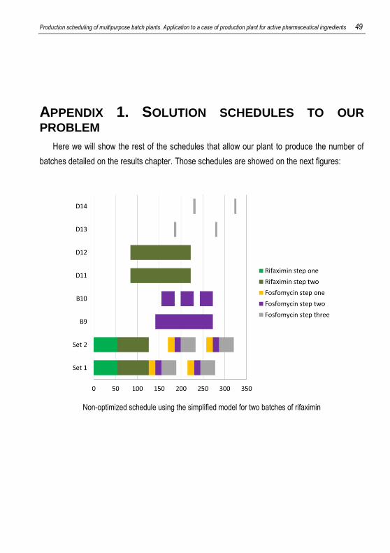
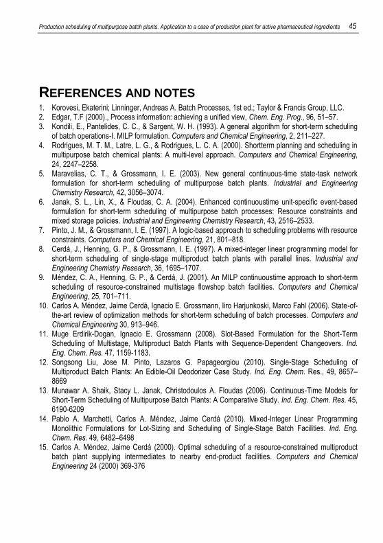
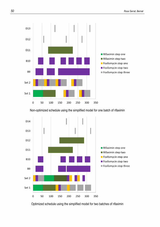
Production scheduling of multipurpose batch plants. Application to a case of production plant for active pharmaceutical ingredients 49
APPENDIX 1. SOLUTION SCHEDULES TO OUR
PROBLEM
Here we will show the rest of the schedules that allow our plant to produce the number of
batches detailed on the results chapter. Those schedules are showed on the next figures:
Non-optimized schedule using the simplified model for two batches of rifaximin
50 Rosa Serrat, Bernat
Non-optimized schedule using the simplified model for one batch of rifaximin
Optimized schedule using the simplified model for two batches of rifaximin
Production scheduling of multipurpose batch plants. Application to a case of production plant for active pharmaceutical ingredients 51
Optimized schedule using the simplified model for a batch of rifaximin
Schedule for production lines using the simplified model
52 Rosa Serrat, Bernat
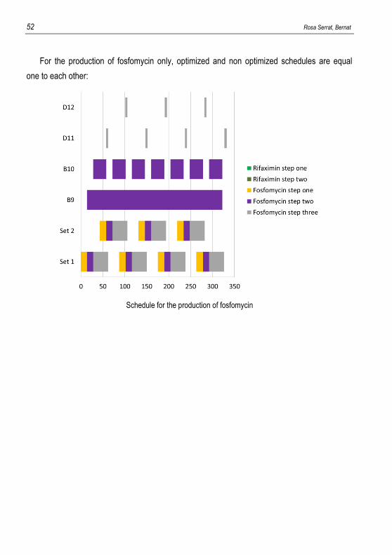
For the production of fosfomycin only, optimized and non optimized schedules are equal
one to each other:
Schedule for the production of fosfomycin

Production scheduling of multipurpose batch plants. Application to a case of production plant for active pharmaceutical ingredients 53
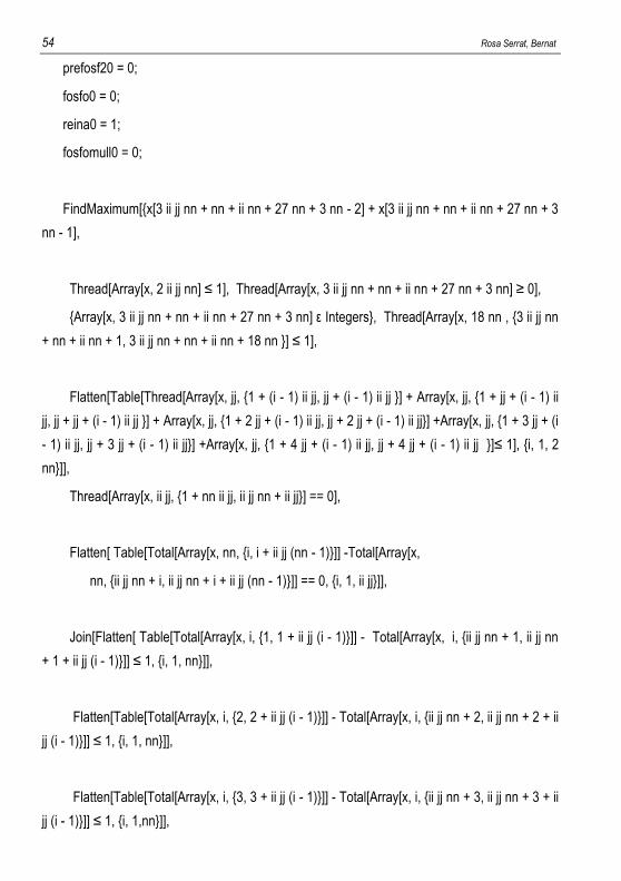
APPENDIX 2. MATHEMATICA PROGRAM
Here is the Mathematica problema used for the resolution of our simplified problem. ii
stands for the number of tasks of the problem, nn the number of time points and jj the number of
available units.
ii = 5;
jj = 2;
nn = 30;
horizon = 336;
alfa1 = 55;
alfa2 = 70;
alfa3 = 14;
alfa4 = 13;
alfa5 = 31;
rifos = 100;
reg = 29;
fosfos = 5;
rifos0 = 0;
rifot0 = 0;
rifomull0 = 0;
prefosf10 = 0;
54 Rosa Serrat, Bernat
prefosf20 = 0;
fosfo0 = 0;
reina0 = 1;
fosfomull0 = 0;
FindMaximum[{x[3 ii jj nn + nn + ii nn + 27 nn + 3 nn - 2] + x[3 ii jj nn + nn + ii nn + 27 nn + 3
nn - 1],
Thread[Array[x, 2 ii jj nn] ≤ 1], Thread[Array[x, 3 ii jj nn + nn + ii nn + 27 nn + 3 nn] ≥ 0],
{Array[x, 3 ii jj nn + nn + ii nn + 27 nn + 3 nn] ε Integers}, Thread[Array[x, 18 nn , {3 ii jj nn
+ nn + ii nn + 1, 3 ii jj nn + nn + ii nn + 18 nn }] ≤ 1],
Flatten[Table[Thread[Array[x, jj, {1 + (i - 1) ii jj, jj + (i - 1) ii jj }] + Array[x, jj, {1 + jj + (i - 1) ii
jj, jj + jj + (i - 1) ii jj }] + Array[x, jj, {1 + 2 jj + (i - 1) ii jj, jj + 2 jj + (i - 1) ii jj}] +Array[x, jj, {1 + 3 jj + (i
- 1) ii jj, jj + 3 jj + (i - 1) ii jj}] +Array[x, jj, {1 + 4 jj + (i - 1) ii jj, jj + 4 jj + (i - 1) ii jj }]≤ 1], {i, 1, 2
nn}]],
Thread[Array[x, ii jj, {1 + nn ii jj, ii jj nn + ii jj}] == 0],
Flatten[ Table[Total[Array[x, nn, {i, i + ii jj (nn - 1)}]] -Total[Array[x,
nn, {ii jj nn + i, ii jj nn + i + ii jj (nn - 1)}]] == 0, {i, 1, ii jj}]],
Join[Flatten[ Table[Total[Array[x, i, {1, 1 + ii jj (i - 1)}]] - Total[Array[x, i, {ii jj nn + 1, ii jj nn
+ 1 + ii jj (i - 1)}]] ≤ 1, {i, 1, nn}]],
Flatten[Table[Total[Array[x, i, {2, 2 + ii jj (i - 1)}]] - Total[Array[x, i, {ii jj nn + 2, ii jj nn + 2 + ii
jj (i - 1)}]] ≤ 1, {i, 1, nn}]],
Flatten[Table[Total[Array[x, i, {3, 3 + ii jj (i - 1)}]] - Total[Array[x, i, {ii jj nn + 3, ii jj nn + 3 + ii
jj (i - 1)}]] ≤ 1, {i, 1,nn}]],
Production scheduling of multipurpose batch plants. Application to a case of production plant for active pharmaceutical ingredients 55
Flatten[Table[Total[Array[x, i, {4, 4 + ii jj (i - 1)}]] - 4Total[Array[x, 4 i, {ii jj nn + 4, 4
ii jj nn + 4 + ii jj (i - 1)}]] ≤ 1, {i, 1, 4nn}]],
Flatten[Table[Total[Array[x, i, {5, 5 + ii jj (i - 1)}]] - Total[Array[x, i, {ii jj nn + 5, ii jj nn + 5 + ii
jj (i - 1)}]] ≤ 1, {i, 1, nn}]],Flatten[Table[Total[Array[x, i, {6, 6 + ii jj (i - 1)}]] - Total[Array[x, i, {ii jj nn
+ 6, ii jj nn + 6 + ii jj (i - 1)}]] ≤ 1, {i, 1, nn}]],
Flatten[Table[Total[Array[x, i, {7, 7 + ii jj (i - 1)}]] - Total[Array[x, i, {ii jj nn + 7, ii jj nn + 7 + ii
jj (i - 1)}]] ≤ 1, {i, 1, nn}]],
Flatten[Table[Total[Array[x, i, {8, 8 + ii jj (i - 1)}]] - Total[Array[x, i, {ii jj nn + 8, i jj nn + 8 + ii
jj (i - 1)}]] ≤ 1, {i, 1, nn}]],
Flatten[Table[Total[Array[x, i, {9, 9 + ii jj (i - 1)}]] - Total[Array[x, i, {ii jj nn + 9, ii jj nn + 9 + ii
jj (i - 1)}]] ≤ 1, {i, 1, nn}]],
Flatten[Table[Total[Array[x, i, {10, 10 + ii jj (i - 1)}]] - Total[Array[x, i, {ii jj nn + 10, ii jj nn +
10 + ii jj (i - 1)}]] ≤ 1, {i, 1, nn}]]],
Join[Flatten[Table[Total[Array[x, i, {1, 1 + ii jj (i - 1)}]] - Total[Array[x, i, {ii jj nn + 1, ii jj nn +
1 + ii jj (i - 1)}]] ≥ 0, {i, 1, nn}]],
Flatten[Table[Total[Array[x, i, {2, 2 + ii jj (i - 1)}]] - Total[Array[x, i, {ii jj nn + 2, ii jj nn + 2 + ii
jj (i - 1)}]] ≥ 0, {i, 1, nn}]],
Flatten[Table[Total[Array[x, i, {3, 3 + ii jj (i - 1)}]] - Total[Array[x, i, {ii jj nn + 3, ii jj nn + 3 + ii
jj (i - 1)}]] ≥ 0, {i, 1, nn}]],
56 Rosa Serrat, Bernat
Flatten[Table[Total[Array[x, i, {4, 4 + ii jj (i - 1)}]] - Total[Array[x, i, {ii jj nn + 4, ii jj nn + 4 + ii jj
(i - 1)}]] ≥ 0, {i, 1, nn}]],
Flatten[Table[Total[Array[x, i, {5, 5 + ii jj (i - 1)}]] - otal[Array[x, i, {ii jj nn + 5, ii jj nn + 5 + ii jj
(i - 1)}]] ≥ 0, {i, 1, nn}]],
Flatten[Table[Total[Array[x, i, {6, 6 + ii jj (i - 1)}]] - Total[ Array[x, i, {ii jj nn + 6,ii jj nn + 6 + ii
jj (i - 1)}]] ≥ 0, {i, 1, nn}]],
Flatten[Table[Total[Array[x, i, {7, 7 + ii jj (i - 1)}]] - Total[Array[x, i, {ii jj nn + 7,
ii jj nn + 7 + ii jj (i - 1)}]] ≥ 0, {i,1, nn}]],
Flatten[
Table[Total[Array[x, i, {8, 8 + ii jj (i - 1)}]] - Total[Array[x,
i, {ii jj nn + 8, ii jj nn + 8 + ii jj (i - 1)}]] ≥ 0, {i,1, nn}]],
Flatten[ Table[Total[Array[x, i, {9, 9 + ii jj (i - 1)}]] - Total[Array[x,
i, {ii jj nn + 9, ii jj nn + 9 + ii jj (i - 1)}]] ≥ 0, {i, 1, nn}]],
Flatten[
Table[Total[Array[x, i, {10, 10 + ii jj (i - 1)}]] - Total[Array[x, i, {ii jj nn + 10, ii jj nn + 10 + ii
jj (i - 1)}]] ≥ 0, {i, 1, nn}]]],
Join[Flatten[ Table[Total[Array[x, i ii, {1, i ii jj - 1}]] - Total[Array[x, i ii, {ii jj nn + 1, ii jj nn +
i ii jj - 1}]] ≤ 1, {i, 1, nn}]], Flatten[ Table[Total[Array[x, i ii, {2, i ii jj}]] - Total[Array[x, i ii, {ii jj nn +
2, ii jj nn + i ii jj}]] ≤
1, {i, 1, nn}]], Flatten[ Table[Total[Array[x, i ii, {1, i ii jj - 1}]] - Total[Array[x, i ii, {ii jj nn + 1,
ii jj nn + i ii jj - 1}]] ≥ 0, {i, 1,
Production scheduling of multipurpose batch plants. Application to a case of production plant for active pharmaceutical ingredients 57
nn}]], Flatten[ Table[Total[Array[x, i ii, {2, i ii jj}]] - Total[Array[x, i ii, {ii jj nn + 2, ii jj nn +
i ii jj}]] ≥ 0, {i, 1, nn}]]],
x[3 ii jj nn + 1 + ii nn] == 0,
x[3 ii jj nn + nn + ii nn] == horizon,
Thread[Array[x, nn ii jj, {2 ii jj nn + 1, 3 ii jj nn}] ≤ x[3 ii jj nn + nn + ii nn]],
Thread[Array[x, nn - 1, {3 ii jj nn + 1 + ii nn, 3 ii jj nn + nn - 1 + ii nn}] ≤ Array[x, nn - 1,
{3 ii jj nn + 2 + ii nn, 3 ii jj nn + nn + ii nn}]],
Flatten[ Table[Thread[ Array[x, ii jj, {1 + 2 ii nn jj + i ii jj, 2 ii nn jj + (i + 1) ii jj}] -
Array[x, ii jj, {1 + 2 ii nn jj + (i - 1) ii jj, 2 ii nn jj + i ii jj}] ≤ horizon Array[x, ii jj, {1 + i ii jj, (i + 1)
ii jj}]], {i, 1, nn - 1}]],
Flatten[ Table[Thread[-Array[x, ii jj, {1 + 2 ii nn jj + i ii jj, 2 ii nn jj + (i + 1) ii jj}] + Array[x, ii
jj, {1 + 2 ii nn jj + (i - 1) ii jj, 2 ii nn jj + i ii jj}] ≤ horizon Array[x, ii jj, {1 + i ii jj, (i + 1) ii jj}]], {i, 1,
nn - 1}]],
Join[Flatten[ Table[Thread[ Array[x, jj, {2 ii jj nn + 1 + (i - 1) ii jj}] ≤ x[3 ii nn jj + ii nn + i] +
horizon (1 -
Array[x, jj, {nn jj ii + 1 + (i - 1) ii jj, nn jj ii + jj + (i - 1) ii jj}])], {i, 1, nn}]], Flatten[Table[
Thread[Array[x, jj, {2 ii jj nn + 1 + jj + (i - 1) ii jj}] ≤ x[3 ii nn jj + ii nn + i] + horizon (1 - Array[x,
jj, {nn jj ii + jj + 1 + (i - 1) ii jj, nn jj ii + jj + jj + (i - 1) ii jj}]) ], {i, 1, nn}]], Flatten[ Table[Thread[
Array[x,
jj, {2 ii jj nn + 1 + 2 jj + (i - 1) ii jj}] ≤ x[3 ii nn jj + ii nn + i] + horizon (1 - Array[x, jj, {nn jj
ii + 2 jj + 1 + (i - 1) ii jj,
nn jj ii + jj + 2 jj + (i - 1) ii jj}]) ], {i, 1, nn}]], Flatten[Table[ Thread[Array[x, jj, {2 ii jj nn +
1 + 3 jj + (i - 1) ii jj}] ≤ x[3 ii nn jj + ii nn + i] + horizon (1 - Array[x, jj, {nn jj ii + 3 jj + 1 + (i - 1)
58 Rosa Serrat, Bernat
ii jj, nn jj ii + jj + 3 jj + (i - 1) ii jj}]) ], {i, 1, nn}]], Flatten[Table[ Thread[Array[x, jj, {2 ii jj nn +
1 +
4 jj + (i - 1) ii jj}] ≤ x[3 ii nn jj + ii nn + i] + horizon (1 - Array[x, jj, {nn jj ii + 4 jj + 1 + (i -
1) ii jj,
nn jj ii + jj + 4 jj + (i - 1) ii jj}]) ], {i, 1, nn}]]],
Join[Flatten[ Table[Thread[ Array[x, jj, {2 ii jj nn + 1 + (i - 1) ii jj, 2 ii jj nn + jj + (i - 1) ii jj}]
≤
x[3 ii jj nn + ii nn + i] + alfa1 Array[x, jj, {1 + (i - 1) ii jj, jj + (i - 1) ii jj}] + horizon (1 -
Array[x, jj, {1 + (i - 1) ii jj, jj + (i - 1) ii jj}])], {i, 1, nn}]], Flatten[ Table[Thread[ Array[x,
jj, {2 ii jj nn + 1 + jj + (i - 1) ii jj, 2 ii jj nn + jj + jj + (i - 1) ii jj}] ≤ x[3 ii jj nn + ii nn + i] +
alfa2 Array[x, jj, {1 + (i - 1) ii jj + jj, jj + jj + (i - 1) ii jj}] + horizon (1 - Array[x, jj, {1 + (i - 1) ii jj
+ jj,
jj + jj + (i - 1) ii jj}])], {i, 1, nn}]], Flatten[Table[ Thread[Array[x, jj, {2 ii jj nn + 1 + 2 jj + (i
- 1) ii jj,
2 ii jj nn + 2 jj + jj + (i - 1) ii jj}] ≤ x[3 ii jj nn + ii nn + i] + alfa3 Array[x, jj, {1 + (i - 1) ii jj + 2
jj, jj + 2 jj + (i - 1) ii jj}] +
horizon (1 - Array[x, jj, {1 + (i - 1) ii jj + 2 jj, jj + 2 jj + (i - 1) ii jj}])], {i, 1, nn}]],
Flatten[Table[
Thread[Array[x, jj, {2 ii jj nn + 1 + 3 jj + (i - 1) ii jj, 2 ii jj nn + 3 jj + jj + (i - 1) ii jj}] ≤ x[3 ii jj
nn + ii nn + i] +
alfa4 Array[x, jj, {1 + (i - 1) ii jj + 3 jj, jj + 3 jj + (i - 1) ii jj}] + horizon (1 - Array[x, jj, {1 +
(i - 1) ii jj + 3 jj,
jj + 3 jj + (i - 1) ii jj}])], {i, 1, nn}]], Flatten[Table[ Thread[Array[x, jj, {2 ii jj nn + 1 + 4 jj +
(i - 1) ii jj,
2 ii jj nn + 4 jj + jj + (i - 1) ii jj}] ≤ x[3 ii jj nn + ii nn + i] + alfa5 Array[x, jj, {1 + (i - 1) ii jj + 4
jj, jj + 4 jj + (i - 1) ii jj}] +
horizon (1 - Array[x, jj, {1 + (i - 1) ii jj + 4 jj, jj + 4 jj + (i - 1) ii jj}])], {i, 1, nn}]]],
Production scheduling of multipurpose batch plants. Application to a case of production plant for active pharmaceutical ingredients 59
Join[Flatten[ Table[Thread[ Array[x, jj, {2 ii jj nn + 1 + (i - 1) ii jj, 2 ii jj nn + jj + (i - 1) ii
jj}] ≥
x[3 ii jj nn + ii nn + i] + alfa1 Array[x, jj, {1 + (i - 1) ii jj, jj + (i - 1) ii jj}] - horizon (1 -
Array[x, jj, {1 + (i - 1) ii jj, jj + (i - 1) ii jj}])], {i, 1, nn}]], Flatten[ Table[Thread[ Array[x,
jj, {2 ii jj nn + 1 + jj + (i - 1) ii jj,
2 ii jj nn + jj + jj + (i - 1) ii jj}] ≥ x[3 ii jj nn + ii nn + i] + alfa2 Array[x, jj, {1 + (i - 1) ii jj + jj, jj
+ (i - 1) ii jj + jj}] -
horizon (1 - Array[x, jj, {1 + (i - 1) ii jj + jj, jj + (i - 1) ii jj + jj}])], {i, 1, nn}]],
Flatten[Table[
Thread[Array[x, jj, {2 ii jj nn + 1 + 2 jj + (i - 1) ii jj, 2 ii jj nn + 2 jj + jj + (i - 1) ii jj}] ≥ x[3 ii
jj nn + ii nn + i] +
alfa3 Array[x, jj, {1 + (i - 1) ii jj + 2 jj, jj + (i - 1) ii jj + 2 jj}] - horizon (1 - Array[x, jj, {1 + (i
- 1) ii jj + 2 jj,
jj + (i - 1) ii jj + 2 jj}])], {i, 1, nn}]], Flatten[Table[ Thread[Array[x, jj, {2 ii jj nn + 1 + 3 jj +
(i - 1) ii jj,
2 ii jj nn + 3 jj + jj + (i - 1) ii jj}] ≥ x[3 ii jj nn + ii nn + i] + alfa4 Array[x, jj, {1 + (i - 1) ii jj +
3 jj, jj + (i - 1) ii jj + 3 jj}] -
horizon (1 - Array[x, jj, {1 + (i - 1) ii jj + 3 jj, jj + (i - 1) ii jj + 3 jj}])], {i, 1, nn}]],
Flatten[Table[
Thread[Array[x, jj, {2 ii jj nn + 1 + 4 jj + (i - 1) ii jj, 2 ii jj nn + jj + 4 jj + (i - 1) ii jj}] ≥ x[3 ii
jj nn + ii nn + i] +
alfa5 Array[x, jj, {1 + (i - 1) ii jj + 4 jj, jj + (i - 1) ii jj + 4 jj}] - horizon (1 - Array[x, jj, {1 + (i
- 1) ii jj + 4 jj,
jj + (i - 1) ii jj + 4 jj}])], {i, 1, nn}]]],
Thread[Array[x, 1, {3 ii jj nn + 1, 3 ii jj nn + 1}] == rifot0 + Total[Array[x, jj, {ii jj nn + 1, ii jj nn
+ jj}]] - Total[Array[x, jj, {3, 2 jj}]]],
60 Rosa Serrat, Bernat
Thread[Array[x, 1, {3 ii jj nn + 2, 3 ii jj nn + 2}] == rifomull0 + Total[Array[x, jj, {ii jj nn + 3, ii
jj nn + jj + 2}]] – Total[Array[x, 4, {3 ii jj nn + nn + ii nn + 1, 3 ii jj nn + nn + ii nn + 4}]]],
Thread[Array[x, 1, {3 ii jj nn + 3, 3 ii jj nn + 3}] == prefosf10 + Total[Array[x, jj, {ii jj nn + 5,
ii jj nn + jj + 4}]] -
Total[Array[x, jj, {9, 5 jj}]]],
Thread[Array[x, 1, {3 ii jj nn + 4, 3 ii jj nn + 4}] == prefosf20 + Total[Array[x, jj, {ii jj nn + 7,
ii jj nn + jj + 6}]] -
Total[Array[x, jj, {9, 5 jj}]]],
Thread[Array[x, 1, {3 ii jj nn + 5, 3 ii jj nn + 5}] == fosfomull0 + Total[Array[x, jj, {ii jj nn +
9, ii jj nn + jj + 8}]] - Total[Array[x, 4, {3 ii jj nn + nn + ii nn + 5, 3 ii jj nn + nn + ii nn + 8}]]],
Flatten[ Table[Thread[ Array[x, 1, {3 ii jj nn + (i - 1) ii + 1, 3 ii jj nn + (i - 1) ii + 1}] ==
x[3 ii jj nn + 1 + (i - 2) ii] +
Total[Array[x, jj, {ii jj nn + 1 + ii jj (i - 1), ii jj nn + jj + ii jj (i - 1)}]] - Total[Array[x, jj, {3 + ii
jj (i - 1), 2 jj + ii jj (i - 1)}]]], {i, 2,
nn}]],
Flatten[ Table[Thread[ Array[x, 1, {3 ii jj nn + (i - 1) ii + 2, 3 ii jj nn + (i - 1) ii + 2}] ==
Array[x,
1, {3 ii jj nn + ii (i - 2) + 2, 3 ii jj nn + ii (i - 2) + 2}] + Total[Array[x, jj, {ii jj nn + 3 + ii jj (i -
1),
ii jj nn + 2 + jj + ii jj (i - 1)}]] - Total[Array[x, 4, {3 ii jj nn + nn + ii nn + 1 + (i - 1) 9, 3 ii jj nn
+ nn + ii nn + 4 + (i - 1) 9}]]], {i, 2, nn}]],
Flatten[ Table[Thread[ x[3 ii jj nn + 3 + (i - 1) ii] == x[3 ii jj nn + 3 + (i - 2) ii] +
Total[Array[x,
Production scheduling of multipurpose batch plants. Application to a case of production plant for active pharmaceutical ingredients 61
jj, {ii jj nn + 5 + ii jj (i - 1), ii jj nn + jj + ii jj (i - 1) + 4}]] - Total[Array[x, jj, {9 + ii jj (i - 1), jj ii
+ ii jj (i - 1)}]]], {i, 2,
nn}]],
Flatten[ Table[Thread[ x[3 ii jj nn + 4 + (i - 1) ii] == x[3 ii jj nn + 4 + (i - 2) ii] +
Total[Array[x,
jj, {ii jj nn + 7 + ii jj (i - 1), ii jj nn + jj + ii jj (i - 1) + 6}]] - Total[Array[x, jj, {9 + ii jj (i - 1), jj ii
+ ii jj (i - 1)}]]], {i, 2,
nn}]],
Flatten[ Table[Thread[ x[3 ii jj nn + 5 + (i - 1) ii] == x[3 ii jj nn + 5 + (i - 2) ii] +
Total[Array[x,
jj, {ii jj nn + 9 + ii jj (i - 1), ii jj nn + jj + ii jj (i - 1) + 8}]] - Total[ Array[x, 4, {3 ii jj nn + nn +
ii nn + 5 + (i - 1) 9,
3 ii jj nn + nn + ii nn + 8 + (i - 1) 9}]]], {i, 2, nn}]],
Flatten[ Table[Thread[ Array[x, 4, {3 ii jj nn + nn + ii nn + 1 + (i - 1) 9, 3 ii jj nn + nn + ii
nn + (i - 1) 9 + 4}] +
Array[x, 4, {3 ii jj nn + nn + ii nn + 5 + (i - 1) 9, 3 ii jj nn + nn + ii nn + (i - 1) 9 + 8}] ≤ 1],
{i, 1, nn}]],
Flatten[ Table[Thread[ Array[x, 1, {3 ii jj nn + nn + ii nn + 9 + (i - 1) 9, 3 ii jj nn + nn + ii
nn + 9 + (i - 1) 9}] ≤
1], {i, 1, nn}]],
Flatten[ Table[Total[ Array[x, nn, {3 ii jj nn + nn + ii nn + i, 3 ii jj nn + nn + ii nn + i + 9
(nn - 1)}]] -
62 Rosa Serrat, Bernat
Total[Array[x, nn, {3 ii jj nn + nn + ii nn + 9 nn + i, 3 ii jj nn + nn + ii nn + i + 9 (nn) + 9
(nn - 1)}]] ==
0, {i, 1, 9}]],
Join[Flatten[ Table[Total[ Array[x, i, {3 ii jj nn + nn + ii nn + 1, 3 ii jj nn + nn + ii nn + 1 +
9 (i - 1)}]] -
Total[ Array[x, i, {3 ii jj nn + nn + ii nn + 9 nn + 1, 3 ii jj nn + nn + ii nn + 9 nn + 1 + 9 (i -
1)}]] ≤ 1, {i, 1, nn}]],
Flatten[ Table[Total[ Array[x, i, {3 ii jj nn + nn + ii nn + 2, 3 ii jj nn + nn + ii nn + 2 + 9 (i -
1)}]] -
Total[Array[x, i, {3 ii jj nn + nn + ii nn + 9 nn + 2, 3 ii jj nn + nn + ii nn + 9 nn + 2 + 9 (i -
1)}]] ≤ 1, {i, 1, nn}]],
Flatten[ Table[Total[ Array[x, i, {3 ii jj nn + nn + ii nn + 3, 3 ii jj nn + nn + ii nn + 3 + 9 (i -
1)}]] - Total[Array[x, i, {3 ii jj nn + nn + ii nn + 9 nn + 3, 3 ii jj nn + nn + ii nn + 9 nn + 3 + 9 (i -
1)}]] ≤ 1, {i, 1, nn}]],
Flatten[ Table[Total[ Array[x, i, {3 ii jj nn + nn + ii nn + 4, 3 ii jj nn + nn + ii nn + 4 + 9 (i -
1)}]] -
Total[Array[x, i, {3 ii jj nn + nn + ii nn + 9 nn + 4, 3 ii jj nn + nn + ii nn + 9 nn + 4 + 9 (i -
1)}]] ≤ 1, {i, 1, nn}]],
Flatten[ Table[Total[ Array[x, i, {3 ii jj nn + nn + ii nn + 5, 3 ii jj nn + nn + ii nn + 5 + 9 (i -
1)}]] -
Total[Array[x, i, {3 ii jj nn + nn + ii nn + 9 nn + 5, 3 ii jj nn + nn + ii nn + 9 nn + 5 + 9 (i -
1)}]] ≤ 1, {i, 1, nn}]],
Flatten[ Table[Total[ Array[x, i, {3 ii jj nn + nn + ii nn + 6, 3 ii jj nn + nn + ii nn + 6 + 9 (i -
1)}]] -
Total[Array[x, i, {3 ii jj nn + nn + ii nn + 9 nn + 6, 3 ii jj nn + nn + ii nn + 9 nn + 6 + 9 (i -
1)}]] ≤ 1, {i, 1, nn}]], Flatten[
Table[Total[ Array[x, i, {3 ii jj nn + nn + ii nn + 7, 3 ii jj nn + nn + ii nn + 7 + 9 (i - 1)}]] -
Total[Array[x,
Production scheduling of multipurpose batch plants. Application to a case of production plant for active pharmaceutical ingredients 63
i, {3 ii jj nn + nn + ii nn + 9 nn + 7, 3 ii jj nn + nn + ii nn + 9 nn + 7 + 9 (i - 1)}]] ≤ 1, {i, 1,
nn}]], Flatten[ Table[Total[ Array[x, i, {3 ii jj nn + nn + ii nn + 8, 3 ii jj nn + nn + ii nn + 8 + 9 (i
- 1)}]] - Total[Array[x, i, {3 ii jj nn + nn + ii nn + 9 nn + 8, 3 ii jj nn + nn + ii nn + 9 nn + 8 + 9
(i - 1)}]] ≤ 1, {i, 1, nn}]], Flatten[ Table[Total[ Array[x, i, {3 ii jj nn + nn + ii nn + 9, 3 ii jj nn +
nn + ii nn + 9 + 9 (i - 1)}]] - Total[Array[x, i, {3 ii jj nn + nn + ii nn + 9 nn + 9, 3 ii jj nn + nn + ii
nn + 9 nn + 9 + 9 (i – 1)}]] ≤ 1, {i, 1, nn}]]],
Join[Flatten[ Table[Total[ Array[x, i, {3 ii jj nn + nn + ii nn + 1, 3 ii jj nn + nn + ii nn + 1 +
9 (i - 1)}]] -
Total[Array[x, i, {3 ii jj nn + nn + ii nn + 9 nn + 1, 3 ii jj nn + nn + ii nn + 9 nn + 1 + 9 (i -
1)}]] ≥ 0, {i, 1, nn}]],
Flatten[ Table[Total[ Array[x, i, {3 ii jj nn + nn + ii nn + 2, 3 ii jj nn + nn + ii nn + 2 + 9 (i -
1)}]] - Total[Array[x, i, {3 ii jj nn + nn + ii nn + 9 nn + 2, 3 ii jj nn + nn + ii nn + 9 nn + 2 + 9 (i -
1)}]] ≥ 0, {i, 1, nn}]],
Flatten[ Table[Total[ Array[x, i, {3 ii jj nn + nn + ii nn + 3, 3 ii jj nn + nn + ii nn + 3 + 9 (i -
1)}]] -
Total[Array[x, i, {3 ii jj nn + nn + ii nn + 9 nn + 3, 3 ii jj nn + nn + ii nn + 9 nn + 3 + 9 (i -
1)}]] ≥ 0, {i, 1, nn}]],
Flatten[ Table[Total[ Array[x, i, {3 ii jj nn + nn + ii nn + 4, 3 ii jj nn + nn + ii nn + 4 + 9 (i -
1)}]] -
Total[Array[x, i, {3 ii jj nn + nn + ii nn + 9 nn + 4, 3 ii jj nn + nn + ii nn + 9 nn + 4 + 9 (i -
1)}]] ≥ 0, {i, 1, nn}]],
Flatten[ Table[Total[ Array[x, i, {3 ii jj nn + nn + ii nn + 5, 3 ii jj nn + nn + ii nn + 5 + 9 (i -
1)}]] -
Total[Array[x, i, {3 ii jj nn + nn + ii nn + 9 nn + 5, 3 ii jj nn + nn + ii nn + 9 nn + 5 + 9 (i -
1)}]] ≥ 0, {i, 1, nn}]],
Flatten[ Table[Total[ Array[x, i, {3 ii jj nn + nn + ii nn + 6, 3 ii jj nn + nn + ii nn + 6 + 9 (i -
1)}]] -
64 Rosa Serrat, Bernat
Total[Array[x, i, {3 ii jj nn + nn + ii nn + 9 nn + 6, 3 ii jj nn + nn + ii nn + 9 nn + 6 + 9 (i -
1)}]] ≥ 0, {i, 1, nn}]],
Flatten[ Table[Total[ Array[x, i, {3 ii jj nn + nn + ii nn + 7, 3 ii jj nn + nn + ii nn + 7 + 9 (i -
1)}]] -
Total[Array[x, i, {3 ii jj nn + nn + ii nn + 9 nn + 7, 3 ii jj nn + nn + ii nn + 9 nn + 7 + 9 (i -
1)}]] ≥ 0, {i, 1, nn}]],
Flatten[ Table[Total[ Array[x, i, {3 ii jj nn + nn + ii nn + 8, 3 ii jj nn + nn + ii nn + 8 + 9 (i -
1)}]] -
Total[Array[x, i, {3 ii jj nn + nn + ii nn + 9 nn + 8, 3 ii jj nn + nn + ii nn + 9 nn + 8 + 9 (i -
1)}]] ≥ 0, {i, 1, nn}]],
Flatten[ Table[Total[ Array[x, i, {3 ii jj nn + nn + ii nn + 9, 3 ii jj nn + nn + ii nn + 9 + 9 (i -
1)}]] -
Total[Array[x, i, {3 ii jj nn + nn + ii nn + 9 nn + 9, 3 ii jj nn + nn + ii nn + 9 nn + 9 + 9 (i -
1)}]] ≥ 0, {i, 1, nn}]]],
Flatten[ Table[Thread[ Array[x, 9, {3 ii jj nn + nn + ii nn + 1 + 2 9 nn + i 9, 3 ii jj nn +
nn + ii nn + 2 9 nn + (i + 1) 9}] -
Array[x, 9, {3 ii jj nn + nn + ii nn + 1 + 2 nn 9 + (i - 1) 9, 3 ii jj nn + nn + ii nn + 2 9 nn + i
9}] ≤
horizon Array[x, 9, {3 ii jj nn + nn + ii nn + 1 + i 9, 3 ii jj nn + nn + ii nn + (i + 1) 9}]], {i, 1,
nn - 1}]],
Flatten[ Table[Thread[-Array[x, 9, {3 ii jj nn + nn + ii nn + 1 + 2 9 nn + i 9, 3 ii jj nn + nn
+ ii nn + 2 9 nn + (i + 1) 9}] +
Array[x, 9, {3 ii jj nn + nn + ii nn + 1 + 2 9 nn + (i - 1) 9, 3 ii jj nn + nn + ii nn + 2 9 nn + i
9}] ≤
horizon Array[x, 9, {3 ii jj nn + nn + ii nn + 1 + 1 + i 9, 3 ii jj nn + nn + ii nn + 1 + (i + 1)
9}]], {i, 1, nn - 1}]],
Join[Flatten[ Table[Thread[ Array[x, 4, {3 ii jj nn + nn + ii nn + 2 9 nn + 1 + (i - 1) 9}] ≤
x[3 ii nn jj + ii nn + i] +
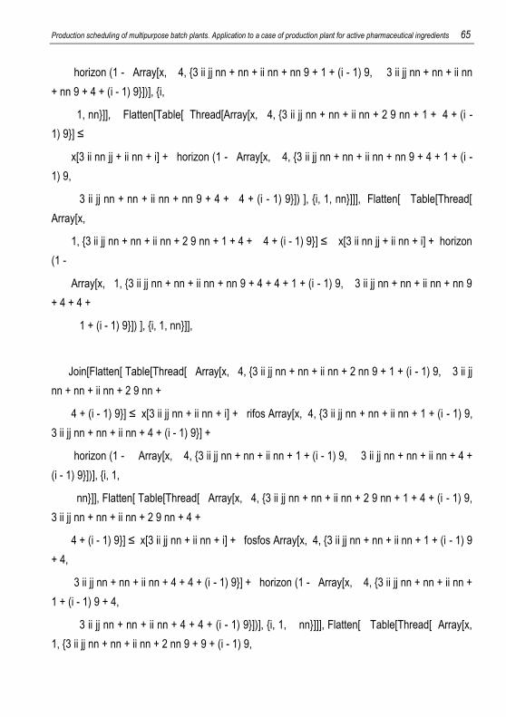
Production scheduling of multipurpose batch plants. Application to a case of production plant for active pharmaceutical ingredients 65
horizon (1 - Array[x, 4, {3 ii jj nn + nn + ii nn + nn 9 + 1 + (i - 1) 9, 3 ii jj nn + nn + ii nn
+ nn 9 + 4 + (i - 1) 9}])], {i,
1, nn}]], Flatten[Table[ Thread[Array[x, 4, {3 ii jj nn + nn + ii nn + 2 9 nn + 1 + 4 + (i -
1) 9}] ≤
x[3 ii nn jj + ii nn + i] + horizon (1 - Array[x, 4, {3 ii jj nn + nn + ii nn + nn 9 + 4 + 1 + (i -
1) 9,
3 ii jj nn + nn + ii nn + nn 9 + 4 + 4 + (i - 1) 9}]) ], {i, 1, nn}]]], Flatten[ Table[Thread[
Array[x,
1, {3 ii jj nn + nn + ii nn + 2 9 nn + 1 + 4 + 4 + (i - 1) 9}] ≤ x[3 ii nn jj + ii nn + i] + horizon
(1 -
Array[x, 1, {3 ii jj nn + nn + ii nn + nn 9 + 4 + 4 + 1 + (i - 1) 9, 3 ii jj nn + nn + ii nn + nn 9
+ 4 + 4 +
1 + (i - 1) 9}]) ], {i, 1, nn}]],
Join[Flatten[ Table[Thread[ Array[x, 4, {3 ii jj nn + nn + ii nn + 2 nn 9 + 1 + (i - 1) 9, 3 ii jj
nn + nn + ii nn + 2 9 nn +
4 + (i - 1) 9}] ≤ x[3 ii jj nn + ii nn + i] + rifos Array[x, 4, {3 ii jj nn + nn + ii nn + 1 + (i - 1) 9,
3 ii jj nn + nn + ii nn + 4 + (i - 1) 9}] +
horizon (1 - Array[x, 4, {3 ii jj nn + nn + ii nn + 1 + (i - 1) 9, 3 ii jj nn + nn + ii nn + 4 +
(i - 1) 9}])], {i, 1,
nn}]], Flatten[ Table[Thread[ Array[x, 4, {3 ii jj nn + nn + ii nn + 2 9 nn + 1 + 4 + (i - 1) 9,
3 ii jj nn + nn + ii nn + 2 9 nn + 4 +
4 + (i - 1) 9}] ≤ x[3 ii jj nn + ii nn + i] + fosfos Array[x, 4, {3 ii jj nn + nn + ii nn + 1 + (i - 1) 9
+ 4,
3 ii jj nn + nn + ii nn + 4 + 4 + (i - 1) 9}] + horizon (1 - Array[x, 4, {3 ii jj nn + nn + ii nn +
1 + (i - 1) 9 + 4,
3 ii jj nn + nn + ii nn + 4 + 4 + (i - 1) 9}])], {i, 1, nn}]]], Flatten[ Table[Thread[ Array[x,
1, {3 ii jj nn + nn + ii nn + 2 nn 9 + 9 + (i - 1) 9,
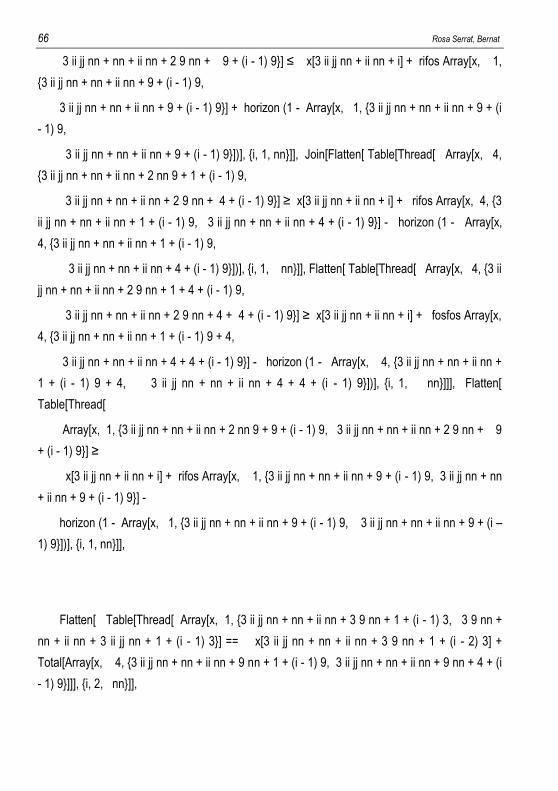
66 Rosa Serrat, Bernat
3 ii jj nn + nn + ii nn + 2 9 nn + 9 + (i - 1) 9}] ≤ x[3 ii jj nn + ii nn + i] + rifos Array[x, 1,
{3 ii jj nn + nn + ii nn + 9 + (i - 1) 9,
3 ii jj nn + nn + ii nn + 9 + (i - 1) 9}] + horizon (1 - Array[x, 1, {3 ii jj nn + nn + ii nn + 9 + (i
- 1) 9,
3 ii jj nn + nn + ii nn + 9 + (i - 1) 9}])], {i, 1, nn}]], Join[Flatten[ Table[Thread[ Array[x, 4,
{3 ii jj nn + nn + ii nn + 2 nn 9 + 1 + (i - 1) 9,
3 ii jj nn + nn + ii nn + 2 9 nn + 4 + (i - 1) 9}] ≥ x[3 ii jj nn + ii nn + i] + rifos Array[x, 4, {3
ii jj nn + nn + ii nn + 1 + (i - 1) 9, 3 ii jj nn + nn + ii nn + 4 + (i - 1) 9}] - horizon (1 - Array[x,
4, {3 ii jj nn + nn + ii nn + 1 + (i - 1) 9,
3 ii jj nn + nn + ii nn + 4 + (i - 1) 9}])], {i, 1, nn}]], Flatten[ Table[Thread[ Array[x, 4, {3 ii
jj nn + nn + ii nn + 2 9 nn + 1 + 4 + (i - 1) 9,
3 ii jj nn + nn + ii nn + 2 9 nn + 4 + 4 + (i - 1) 9}] ≥ x[3 ii jj nn + ii nn + i] + fosfos Array[x,
4, {3 ii jj nn + nn + ii nn + 1 + (i - 1) 9 + 4,
3 ii jj nn + nn + ii nn + 4 + 4 + (i - 1) 9}] - horizon (1 - Array[x, 4, {3 ii jj nn + nn + ii nn +
1 + (i - 1) 9 + 4, 3 ii jj nn + nn + ii nn + 4 + 4 + (i - 1) 9}])], {i, 1, nn}]]], Flatten[
Table[Thread[
Array[x, 1, {3 ii jj nn + nn + ii nn + 2 nn 9 + 9 + (i - 1) 9, 3 ii jj nn + nn + ii nn + 2 9 nn + 9
+ (i - 1) 9}] ≥
x[3 ii jj nn + ii nn + i] + rifos Array[x, 1, {3 ii jj nn + nn + ii nn + 9 + (i - 1) 9, 3 ii jj nn + nn
+ ii nn + 9 + (i - 1) 9}] -
horizon (1 - Array[x, 1, {3 ii jj nn + nn + ii nn + 9 + (i - 1) 9, 3 ii jj nn + nn + ii nn + 9 + (i –
1) 9}])], {i, 1, nn}]],
Flatten[ Table[Thread[ Array[x, 1, {3 ii jj nn + nn + ii nn + 3 9 nn + 1 + (i - 1) 3, 3 9 nn +
nn + ii nn + 3 ii jj nn + 1 + (i - 1) 3}] == x[3 ii jj nn + nn + ii nn + 3 9 nn + 1 + (i - 2) 3] +
Total[Array[x, 4, {3 ii jj nn + nn + ii nn + 9 nn + 1 + (i - 1) 9, 3 ii jj nn + nn + ii nn + 9 nn + 4 + (i
- 1) 9}]]], {i, 2, nn}]],
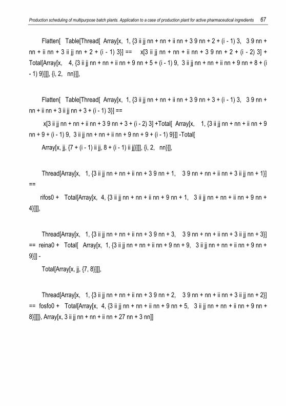
Production scheduling of multipurpose batch plants. Application to a case of production plant for active pharmaceutical ingredients 67
Flatten[ Table[Thread[ Array[x, 1, {3 ii jj nn + nn + ii nn + 3 9 nn + 2 + (i - 1) 3, 3 9 nn +
nn + ii nn + 3 ii jj nn + 2 + (i - 1) 3}] == x[3 ii jj nn + nn + ii nn + 3 9 nn + 2 + (i - 2) 3] +
Total[Array[x, 4, {3 ii jj nn + nn + ii nn + 9 nn + 5 + (i - 1) 9, 3 ii jj nn + nn + ii nn + 9 nn + 8 + (i
- 1) 9}]]], {i, 2, nn}]],
Flatten[ Table[Thread[ Array[x, 1, {3 ii jj nn + nn + ii nn + 3 9 nn + 3 + (i - 1) 3, 3 9 nn +
nn + ii nn + 3 ii jj nn + 3 + (i - 1) 3}] ==
x[3 ii jj nn + nn + ii nn + 3 9 nn + 3 + (i - 2) 3] +Total[ Array[x, 1, {3 ii jj nn + nn + ii nn + 9
nn + 9 + (i - 1) 9, 3 ii jj nn + nn + ii nn + 9 nn + 9 + (i - 1) 9}]] -Total[
Array[x, jj, {7 + (i - 1) ii jj, 8 + (i - 1) ii jj}]]], {i, 2, nn}]],
Thread[Array[x, 1, {3 ii jj nn + nn + ii nn + 3 9 nn + 1, 3 9 nn + nn + ii nn + 3 ii jj nn + 1}]
==
rifos0 + Total[Array[x, 4, {3 ii jj nn + nn + ii nn + 9 nn + 1, 3 ii jj nn + nn + ii nn + 9 nn +
4}]]],
Thread[Array[x, 1, {3 ii jj nn + nn + ii nn + 3 9 nn + 3, 3 9 nn + nn + ii nn + 3 ii jj nn + 3}]
== reina0 + Total[ Array[x, 1, {3 ii jj nn + nn + ii nn + 9 nn + 9, 3 ii jj nn + nn + ii nn + 9 nn +
9}]] -
Total[Array[x, jj, {7, 8}]]],
Thread[Array[x, 1, {3 ii jj nn + nn + ii nn + 3 9 nn + 2, 3 9 nn + nn + ii nn + 3 ii jj nn + 2}]
== fosfo0 + Total[Array[x, 4, {3 ii jj nn + nn + ii nn + 9 nn + 5, 3 ii jj nn + nn + ii nn + 9 nn +
8}]]]}, Array[x, 3 ii jj nn + nn + ii nn + 27 nn + 3 nn]]

68 Rosa Serrat, Bernat