Embed Size (px)
Citation preview

The water footprint of India A study on water use in relation to the consumption of agricultural goods in the Indian states Master thesis Date: April 2007 Author: D.A. Kampman
Email: [email protected]
Graduation committee: Prof. Dr. Ir. A.Y. Hoekstra (University of Twente)
Dr. Ir. M.S. Krol (University of Twente)


“As I travel around the world, people think the only place where there is potential conflict over water is the Middle East, but they are completely wrong. We have the
problem all over the world. “ (Koffi Annan)
“When the well is dry, we learn the value of water”
(Benjamin Franklin)


Preface The completion of this study means the completion of the Master course Civil Engineering & Management at the University of Twente. I started with the execution of this study in May 2006. After a good start, I got stuck on the many decisional crossroads this subject has to offer and I slowly realised that this study might not shake up the world as much as I had hoped. However, after making some rough decisions, I began to see the light and things started to fall into place. In the last period of this study, I have tried hard to write a comprehensible report on the subject, including a relevant link to the Indian society. And although there is still room for improvements, I am very satisfied with the current result. I would like to thank a number of people without whom this result would not have been possible. First of all, I would like to thank the members of my graduation committee. I would like to thank Arjen Hoekstra for his advice, criticism and ideas, for helping me with the overall direction of the study and for offering me a look in the interesting kitchen of multidisciplinary water management. I would like to thank Maarten Krol for his profound analysis of my concept reports, which undoubtedly increased the scientific value of the study. I would like to thank both Arjen Hoekstra and Maarten Krol for the pleasant collaboration during the execution of this study. I also would like to thank Ashok Chapagain for his sharing his knowledge on the subject. Next, I would like to thank my colleagues at the graduation chamber for their pleasant company, for the discussions in the coffee corner and for sharing the good times and “de uren van nood en ontbering” with me. I also would like to thank my parents for creating a steady base in this life for me, for their advice and for their ever present support. Finally, I would like to thank Rianne for her love, faith and encouragement. Although from a long distance during the weeks, her support has been immensely important to me. Doeke Kampman Enschede, April 2007 Acknowledgement This study has been executed at the University of Twente under the department of Water Engineering & Management between May 2006 and April 2007. I would like to thank the department of Water Engineering & Management for offering me the necessary facilities during this period.


Summary The concept of the water footprint has been developed to create an indicator of water use in relation to the consumption by people. The water footprint of a country is defined as the volume of water needed for the production of the goods and services consumed by the inhabitants of the country. The water footprint is divided into a blue, a green and a gray component. The blue component refers to the evaporation of groundwater and surface water during the production of a commodity, the green component to the evaporation of rain water for crop growth, and the gray component to the water required to dilute the water pollution that is caused by the production of the commodity to acceptable levels. In the next fifty years, India is projected to face the challenge of feeding a population of 1.6 billion people with a higher level of welfare than at present. The current view of the Indian government on food security is to hold on to the goal of food self sufficiency. Knowing that agriculture is the main consumer of water, the implied increase in food demand will increase the pressure on the renewable water resources. In order to reduce the pressure on renewable water resources, the Indian government is considering the concept of river interlinking as the solution for water scarcity in the drier regions. This concept means that water abundant regions will provide water to water scarce regions through the connection of rivers. Whether the interlinking of rivers will provide enough water to solve the observed and future water deficit and what the side effects of the project will be is still unclear. This study indicates why the water scarce regions have a water deficit. In the period 1997‐2001, the water footprint of the inhabitants of the Indian states varied between 451 and 1357 m3/cap/yr with an average of 777 m3/cap/yr. Of this average, 658 m3/cap/yr originated from local water resources and 119 m3/cap/yr from water resources of other states or other nations. Furthermore, the blue component of the average water footprint came to 227 m3/cap/yr, the green component to 459 m3/cap/yr and the gray component to 92 m3/cap/yr. During the study period, the total virtual water flow as a result of interstate trade in agricultural commodities in India was 106 billion m3/yr, which was 13% of the total water use in Indian agriculture. In the same period, the net international export from India was 15 billion m3/yr. Of the total virtual water flow within India, 35% was due to the interstate trade in milled rice, 17% due the interstate trade in raw sugar and 14% due to the interstate trade in edible oils. The largest interregional net virtual water flow was 22 billion m3/yr and flowed from North India to East India. As a result of international and interstate virtual water flows, the states Haryana, Madhya Pradesh, Punjab and Uttar Pradesh had the largest net export of virtual water and Bihar, Jharkhand and Kerala had the largest net import of virtual water. The water scarcity from the perspective of consumption is the highest in the states of Rajasthan, Punjab, Uttar Pradesh, Tamil Nadu and Haryana. This means that the water resources of these states are closest to be exhausted in case of food self sufficiency. Because most of the states are also net exporters of virtual water, the water scarcity from production perspective is even higher in these states. The total net global water saving as a result of the interstate trade in agricultural commodities in India was 41 billion m3/yr. This means the total water use in Indian agriculture was 5%

lower than it would have been without interstate trade. The interstate trade in wheat alone already caused a global water saving of 23 billion m3/yr. Looking at the river interlinking project from the perspective of the virtual water flows as calculated in this study, it can be seen that the proposed water transfer from East to North India has a direction exactly opposite to the direction of the virtual water flow as a result of interstate trade. In this study, it is demonstrated that an increase in water productivity in the water abundant states has a better chance of reducing the national water scarcity than the proposed water transfer. The river interlinking project mainly reduces local water scarcity, while water scarcity needs to be reduced significantly at a national level in order to remain food self sufficient as a nation. The only long term option for reducing the national water scarcity and remaining food self sufficient is to increase the water productivity in India. The largest opportunity for this increase lies in East India, where there is an abundance of water and a large increase in water productivity seems possible.


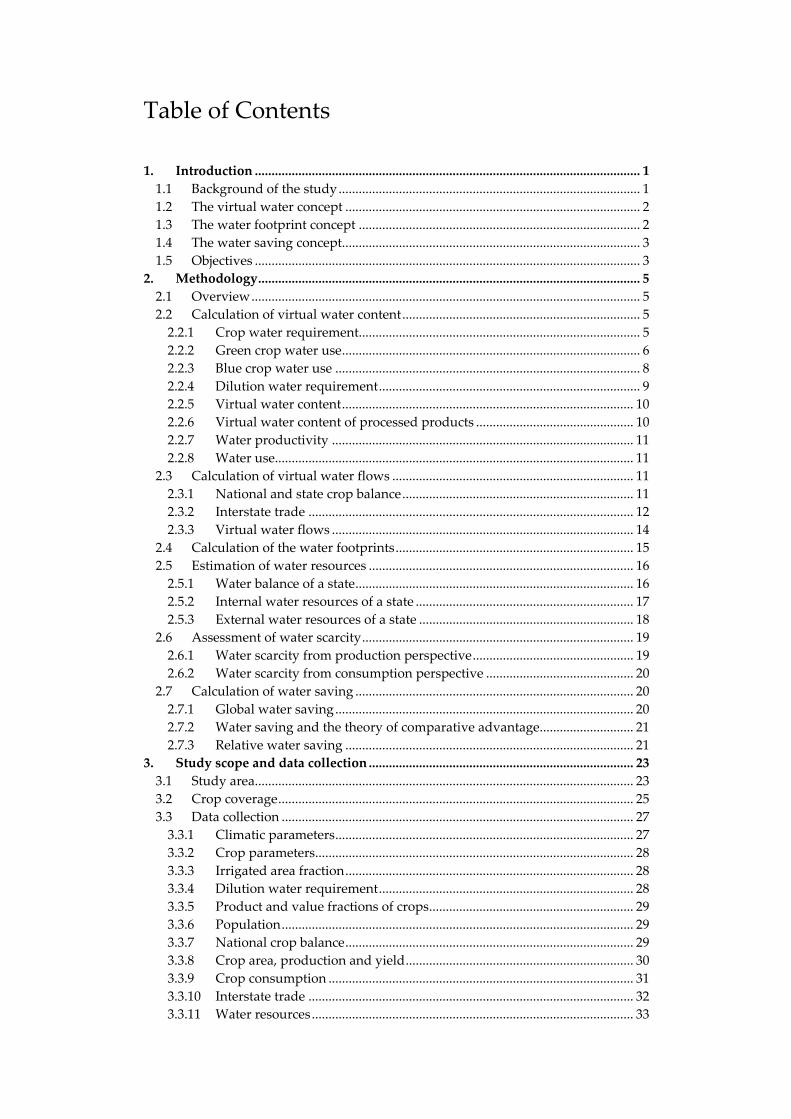
Table of Contents 1. Introduction ................................................................................................................... 1 1.1 Background of the study.......................................................................................... 1 1.2 The virtual water concept ........................................................................................ 2 1.3 The water footprint concept .................................................................................... 2 1.4 The water saving concept......................................................................................... 3 1.5 Objectives ................................................................................................................... 3
2. Methodology.................................................................................................................. 5 2.1 Overview.................................................................................................................... 5 2.2 Calculation of virtual water content....................................................................... 5 2.2.1 Crop water requirement.................................................................................... 5 2.2.2 Green crop water use......................................................................................... 6 2.2.3 Blue crop water use ........................................................................................... 8 2.2.4 Dilution water requirement.............................................................................. 9 2.2.5 Virtual water content....................................................................................... 10 2.2.6 Virtual water content of processed products ............................................... 10 2.2.7 Water productivity .......................................................................................... 11 2.2.8 Water use........................................................................................................... 11
2.3 Calculation of virtual water flows ........................................................................ 11 2.3.1 National and state crop balance..................................................................... 11 2.3.2 Interstate trade ................................................................................................. 12 2.3.3 Virtual water flows .......................................................................................... 14
2.4 Calculation of the water footprints....................................................................... 15 2.5 Estimation of water resources ............................................................................... 16 2.5.1 Water balance of a state................................................................................... 16 2.5.2 Internal water resources of a state ................................................................. 17 2.5.3 External water resources of a state ................................................................ 18
2.6 Assessment of water scarcity................................................................................. 19 2.6.1 Water scarcity from production perspective................................................ 19 2.6.2 Water scarcity from consumption perspective ............................................ 20
2.7 Calculation of water saving ................................................................................... 20 2.7.1 Global water saving......................................................................................... 20 2.7.2 Water saving and the theory of comparative advantage............................ 21 2.7.3 Relative water saving ...................................................................................... 21
3. Study scope and data collection ............................................................................... 23 3.1 Study area................................................................................................................. 23 3.2 Crop coverage.......................................................................................................... 25 3.3 Data collection ......................................................................................................... 27 3.3.1 Climatic parameters......................................................................................... 27 3.3.2 Crop parameters............................................................................................... 28 3.3.3 Irrigated area fraction...................................................................................... 28 3.3.4 Dilution water requirement............................................................................ 28 3.3.5 Product and value fractions of crops............................................................. 29 3.3.6 Population......................................................................................................... 29 3.3.7 National crop balance...................................................................................... 29 3.3.8 Crop area, production and yield.................................................................... 30 3.3.9 Crop consumption ........................................................................................... 31 3.3.10 Interstate trade ................................................................................................. 32 3.3.11 Water resources................................................................................................ 33
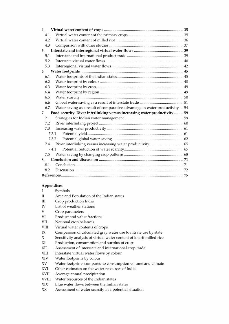
4. Virtual water content of crops .................................................................................. 35 4.1 Virtual water content of the primary crops ......................................................... 35 4.2 Virtual water content of milled rice...................................................................... 36 4.3 Comparison with other studies............................................................................. 37
5. Interstate and interregional virtual water flows ................................................... 39 5.1 Interstate and international product trade .......................................................... 39 5.2 Interstate virtual water flows ................................................................................ 40 5.3 Interregional virtual water flows .......................................................................... 42
6. Water footprints .......................................................................................................... 45 6.1 Water footprints of the Indian states .................................................................... 45 6.2 Water footprint by colour ...................................................................................... 48 6.3 Water footprint by crop.......................................................................................... 49 6.4 Water footprint by region ...................................................................................... 49 6.5 Water scarcity .......................................................................................................... 50 6.6 Global water saving as a result of interstate trade ............................................. 51 6.7 Water saving as a result of comparative advantage in water productivity .... 54
7. Food security: River interlinking versus increasing water productivity.......... 59 7.1 Strategies for Indian water management............................................................. 59 7.2 River interlinking project ....................................................................................... 60 7.3 Increasing water productivity ............................................................................... 61 7.3.1 Potential yield................................................................................................... 61 7.3.2 Potential global water saving ......................................................................... 62
7.4 River interlinking versus increasing water productivity................................... 65 7.4.1 Potential reduction of water scarcity............................................................. 65
7.5 Water saving by changing crop patterns ............................................................. 68 8. Conclusion and discussion ....................................................................................... 71 8.1 Conclusion ............................................................................................................... 71 8.2 Discussion ................................................................................................................ 72
References.............................................................................................................................. 75 Appendices I Symbols II Area and Population of the Indian states III Crop production India IV List of weather stations V Crop parameters VI Product and value fractions VII National crop balances VIII Virtual water contents of crops IX Comparison of calculated gray water use to nitrate use by state X Sensitivity analysis of virtual water content of kharif milled rice XI Production, consumption and surplus of crops XII Assessment of interstate and international crop trade XIII Interstate virtual water flows by colour XIV Water footprints by colour XV Water footprints compared to consumption volume and climate XVI Other estimates on the water resources of India XVII Average annual precipitation XVIII Water resources of the Indian states XIX Blue water flows between the Indian states XX Assessment of water scarcity in a potential situation


1. Introduction
1.1 Background of the study With over one billion people, India currently has the world’s second largest population. The estimate of the amount of people living in India in the year 2050 is 1.6 billion (United Nations, 2004). This is an increase in population of approximately 50% in the next fifty years. Next to this population growth the total Gross Domestic Product (GDP) per capita in India is also growing rapidly (7.1% in 2005 (World Bank, 2006)). Furthermore, there currently is a net export of agricultural products from India, which has shown an increase in the past decade (FAO, 2006a), which is likely to persist. These developments will lead to a large growth in the total food demand in India in the near future. How can India cope with this scenario? Can the production of food be increased? And if so, should India increase its food production or should India import more products from other countries? Since most of the utilizable water supply in India is used for crop production (Hoekstra & Chapagain, 2007), an important criterion for the evaluation of a possible food supply strategy is the pressure on renewable water resources. At the moment there are regions in India that are determined as water scarce, as the water availability per is capita is less than 1000 m3/yr, which is either caused by the lack of natural water resources or a result of over exploitation of groundwater resources for irrigation purposes (CGWB, 1989; Bobba et al., 1997). The pressure on water resources is also increasing through the increase in water pollution caused by diffuse agricultural sources in the form of animal manure, fertilizers and pesticides. While the application of fertilizers and pesticides is currently low compared to developed countries, the intensification of agriculture is bound to cause an increase of diffuse agricultural pollution. The monitoring of groundwater and surface water have currently only resulted in the reporting of high nitrate concentrations in groundwater, which is in most cases linked directly to diffuse agricultural sources (Agrawal, 1999). The current point of view of the Indian government on the topic of food security is to hold on to the goal of national food self sufficiency. The begging bowl image of the sixties is something that is still carved in the minds of the Indian people and is to be prevented at all cost (Gupta & Deshpande, 2004; Planning Commission, 2002). In order to reduce the pressure on the renewable water resources, the Indian government is considering the concept of river interlinking as the solution for water scarcity in the drier regions. This concept means that water abundant regions will provide water to water scarce regions through the connection of rivers (NWDA, 2006). Whether the interlinking of rivers will provide enough water to solve the water deficit and what the side effects of the project will be is still unclear (Radhakrishna, 2003).
1
Water footprint of India Introduction
Since the interlinking of rivers is such an enormous project, it is useful to see to what extent another strategy can reduce the water scarcity in the drier regions.
1.2 The virtual water concept This other water scarcity reducing strategy can be quantitatively described with the concept of virtual water. This concept defines the virtual water content of a commodity as the volume of water that is actually used to produce the commodity, measured at the place where the commodity is actually produced (Allen, 1993, 1994). The inverse of the virtual water content is known as the water productivity of a crop. With the virtual water content, the production and the trade flow of a crop can be translated into the water use and the virtual water flow of crop. So instead of increasing local water resources by importing water, the water use in the water deficit regions can be reduced by an increase in water productivity or a change in the existing trade pattern. The water productivity of a crop can be increased when a significant gap exists between the current and potential water productivity. A change in the existing trade pattern is possible if importing states can increase their crop production and can be become less dependent, self sufficient or even exporters.
1.3 The water footprint concept In line with the concept of virtual water, the concept of the water footprint has been introduced to create a consumption‐based indicator of water use (Hoekstra & Hung, 2004; Hoekstra & Chapagain, 2007). This in contrast to the traditional production‐sector‐based indicators of water use, that are useful in water management but do not indicate the water that is actually needed by the inhabitants of a country in relation to their consumption pattern. The water footprint is defined as the volume of water needed for the production of the goods and services consumed by the inhabitants of a country. This concept is developed in analogy to the concept of the ecological footprint (Wackernagel & Rees, 1996). The water footprint can be divided into an internal and an external water footprint. The internal component covers the use of domestic water resources and the external component covers the use of water resources elsewhere. Furthermore, an agricultural, an industrial and a domestic component of the water footprint can be assessed. Here, the agricultural component corresponds with the water use in the agricultural sector (i.e. in the form of crop evapotranspiration or water pollution), the industrial component corresponds with the water use in the industrial sector and the domestic component with the water use in the domestic sector. Finally, the water footprint can be divided into a blue, a green and a gray water footprint. The blue component covers the use of groundwater and surface water during the production of a commodity, the green component covers the use of rain water for crop growth, and the gray component covers the water required to dilute the water that is polluted during the production of the commodity. The distinction between green and blue water has been introduced by Falkenmark & Rockström (1993). The gray component has been introduced by Chapagain et al. (2006).
2

Water footprint of India Introduction
1.4 The water saving concept With the current water productivity in India and the food demand scenario for the year 2050, it seems inevitable for India to become an importer of virtual water (Falkenmark, 1997; Yang et al., 2003; Falkenmark & Lannerstad, 2005). This is because the average (utilizable) water availability per capita in India will drop below the minimum amount of water needed to feed a person in the near future. This means that water scarcity is not only a local problem in India but also a national problem. Given that the total water resources are more or less fixed, neglecting possible climatic changes, the only way to reduce the national water scarcity is to reduce the total water use with a constant or growing food production. This means that an increase in water productivity is needed together with water saving on a global scale. Global water saving is created when a product that is traded has a higher virtual water content in the importing state than in the exporting state (Chapagain & Hoekstra, 2006). This means that the water loss in the exporting state is lower than the water saving in the importing state. If the water loss as a result of trade is larger than the water saving, there is a global loss.
1.5 Objectives To get more insight on whether the water scarcity in the Indian states is caused by local consumption or by the export of agricultural commodities to other states or countries, the water footprints of the Indian states are assessed in this study. The first target of this study is to assess the international and interstate virtual water flows from and to the Indian states and create a net virtual water balance for each state. In order to assess these virtual water flows, the import, export and virtual water contents of the crops need to be calculated for each Indian state. Because data on crop trade is not directly available at the state level, the trade of a crop is estimated based on the production and consumption volumes per state and the national balance of a crop. The second target is to assess the water footprints related to the consumption of agricultural commodities of the Indian states. This is determined by the water use in the states and the virtual water flows from and to the states. The third target is to assess the water scarcity in the Indian states. To this end, the water resources are estimated by state. Water scarcity is assessed from the production perspective by comparing water availability to the water use in a state, and from the consumption perspective by comparing water availability to the water footprint of a state. The fourth target is to assess global water saving as a result of interstate trade in agricultural commodities. Global water saving is calculated from the difference between the virtual water content of the crop in the importing and exporting state. Global water saving gives an indication of the relative water use efficiency of interstate trade in agricultural commodities in India. The fifth and last target of this study is to compare the river interlinking project to the outcome of the previous objectives. This might give an indication to what extent the local and national water scarcity can be reduced more by water transport through the connection of
3

Water footprint of India Introduction
rivers or by a combination of an increase in water productivity and a change in interstate trade patterns. The period of analysis in this study is 1997‐2001, because this is the most recent five‐year period for which all necessary data could be obtained. The scope of the study is limited to agricultural commodities, since they are responsible for the major part of global water use (Postel et al., 1996). Livestock products are not taken into account, because they are more difficult to assess and generally contribute a small part to the total trade in virtual water (Chapagain & Hoekstra, 2003).
4

2. Methodology
2.1 Overview The starting point in this methodology is the calculation of the green, blue and gray virtual water content of a crop by season and by state. This calculation is derived from a method used by Chapagain et al. (2006). The following step is the estimation of the international and interstate trade of a crop by state. This estimation is based on the method used by Ma et al. (2006). With the virtual water contents, the crop production of a state is translated into the water use of a state and the interstate crop trade of a state into the virtual water flow of a state. The total water use and the gross virtual water flows of a state determine the water footprint of a state. Next, the water resources of the Indian states are estimated. Together with the water footprint, the water resources give an indication of the water scarcity in the Indian states. Finally, the global water saving as a result of interstate trade is calculated. Throughout this chapter, independent variable c denotes crop, s state, t time steps of 10 days, p agricultural product, rb river basin and us upstream state. A summary of all used symbols in this study is presented in Appendix I.
2.2 Calculation of virtual water content
2.2.1 Crop water requirement The calculation of the virtual water content of a crop starts with the calculation of the volume of water that is required for the crop growth. Crop water requirement (CWR, m3/ha) is defined as the volume of water that is required to compensate the water loss of a crop through evapotranspiration under growth conditions with no constraint by water shortage (Allen et al., 1998). The CWR is calculated by accumulating the data on the crop evapotranspiration under optimal conditions (ETc,opt, mm/day) over the complete growing period.
[ ] [ tscETscCWRlp
toptc ,,10,
1,∑
=
∗= ] (1)
Here, the factor 10 is included to convert mm into m3/ha and the summation is done in time steps of 10 days over the full growing period lp. It is worth noticing that in this calculation each month is taken to be equal to 3 time steps of 10 days, which means that all months are assumed to consist of exactly 30 days. The ETc, opt is calculated as follows:
5
Water footprint of India Methodology
[ ] [ ] [sETcKscET ocoptc ∗ ]=,, (2)
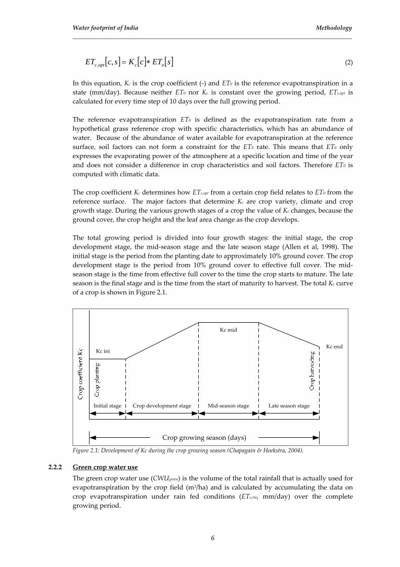
In this equation, Kc is the crop coefficient (‐) and ET0 is the reference evapotranspiration in a state (mm/day). Because neither ET0 nor Kc is constant over the growing period, ETc,opt is calculated for every time step of 10 days over the full growing period. The reference evapotranspiration ET0 is defined as the evapotranspiration rate from a hypothetical grass reference crop with specific characteristics, which has an abundance of water. Because of the abundance of water available for evapotranspiration at the reference surface, soil factors can not form a constraint for the ET0 rate. This means that ET0 only expresses the evaporating power of the atmosphere at a specific location and time of the year and does not consider a difference in crop characteristics and soil factors. Therefore ET0 is computed with climatic data. The crop coefficient Kc determines how ETc,opt from a certain crop field relates to ET0 from the reference surface. The major factors that determine Kc are crop variety, climate and crop growth stage. During the various growth stages of a crop the value of Kc changes, because the ground cover, the crop height and the leaf area change as the crop develops. The total growing period is divided into four growth stages: the initial stage, the crop development stage, the mid‐season stage and the late season stage (Allen et al, 1998). The initial stage is the period from the planting date to approximately 10% ground cover. The crop development stage is the period from 10% ground cover to effective full cover. The mid‐season stage is the time from effective full cover to the time the crop starts to mature. The late season is the final stage and is the time from the start of maturity to harvest. The total Kc curve of a crop is shown in Figure 2.1.
Crop growing season (days)
Crop development stage Mid‐season stage Late season stageInitial stage
Kc ini
Kc mid
Kc end
Figure 2.1: Development of Kc during the crop growing season (Chapagain & Hoekstra, 2004).
2.2.2 Green crop water use The green crop water use (CWUgreen) is the volume of the total rainfall that is actually used for evapotranspiration by the crop field (m3/ha) and is calculated by accumulating the data on crop evapotranspiration under rain fed conditions (ETc,rw, mm/day) over the complete growing period.
6

Water footprint of India Methodology
[ ] [ tscETscCWUlp
trwcgreen ,,*10,
1,∑
=
= ] (3)
As in the calculation of the CWR, the factor 10 is included to convert mm into m3/ha and the summation is done over the full growth period lp (day) in time steps of 10 days. The ETc,rw is determined as follows:
[ ] [ ] [ ]),,(, ,, sPscETMinscET effoptcrwc = (4)
Here, Peff is the effective rainfall (mm/day), which is defined as the amount of the total precipitation (Ptot, mm/day) that can be used for evapotranspiration by the crop and the soil surface. Equation 4 shows that ETc,rw is equal to Peff if Peff is lower than ETc,opt, and that ETc,rw is equal to ETc,opt if Peff is higher than ETc,opt. This is because a crop uses as much water as possible for ETc,opt, but never uses more water than it requires for optimal growth. The fact that in some time steps a part of the Peff is not used for evapotranspiration, and is thus still available as soil moisture for a following time step, is not taken into account in this study. The effective rainfall Peff is generated from Ptot by CROPWAT (FAO, 2006b). CROPWAT calculates with a simplified version of the USDA method. This is a simplification because the soil type and the net depth of irrigation application are not taken into account in this method (Dastane, 1978). The simplified method consists of equations 5 and 6. The factor 30 is added to these equations, because the original equations assume monthly values instead of daily values. The relation between Peff and Ptot that is created by these equations is presented in Figure 2.2.
)2.030
125(12530
30250
tottotefftot PPPP ∗−∗∗=→≤ (5)
totefftot PPP ∗+=→> 1.030
12530250
(6)
012345678910
0 1 2 3 4 5 6 7 8 9 10
Total rainfall (mm/day)
250/30 ≈ 8.3Ptot
Peff
Effective rainfall (m
m/day)
Figure 2.2: The relation between effective rainfall and total rainfall
7
Water footprint of India Methodology
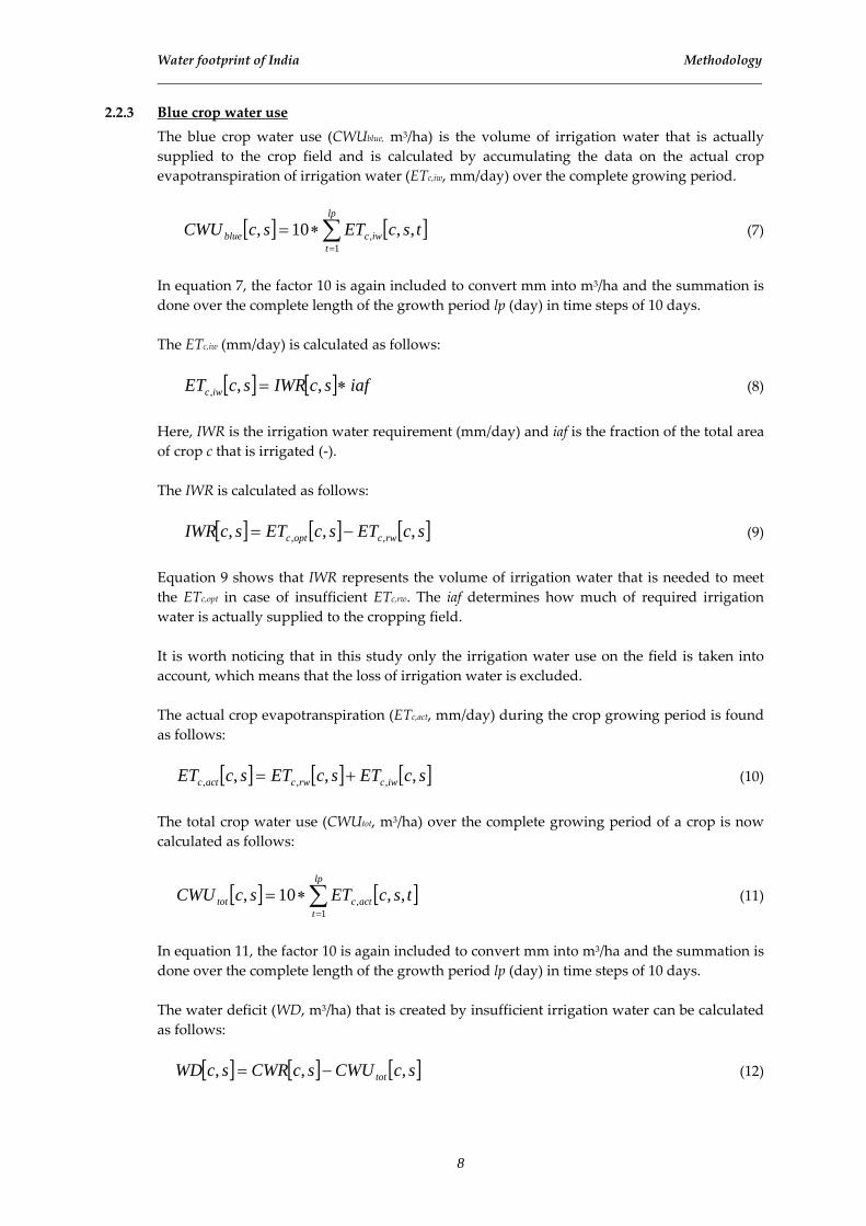
2.2.3 Blue crop water use The blue crop water use (CWUblue, m3/ha) is the volume of irrigation water that is actually supplied to the crop field and is calculated by accumulating the data on the actual crop evapotranspiration of irrigation water (ETc,iw, mm/day) over the complete growing period.
[ ] [ tscETscCWUlp
tiwcblue ,,10,
1,∑
=
∗= ] (7)
In equation 7, the factor 10 is again included to convert mm into m3/ha and the summation is done over the complete length of the growth period lp (day) in time steps of 10 days. The ETc,iw (mm/day) is calculated as follows:
[ ] [ ] iafscIWRscET iwc ∗= ,,, (8)
Here, IWR is the irrigation water requirement (mm/day) and iaf is the fraction of the total area of crop c that is irrigated (‐). The IWR is calculated as follows:
[ ] [ ] [ ]scETscETscIWR rwcoptc ,,, ,, −= (9)
Equation 9 shows that IWR represents the volume of irrigation water that is needed to meet the ETc,opt in case of insufficient ETc,rw. The iaf determines how much of required irrigation water is actually supplied to the cropping field. It is worth noticing that in this study only the irrigation water use on the field is taken into account, which means that the loss of irrigation water is excluded. The actual crop evapotranspiration (ETc,act, mm/day) during the crop growing period is found as follows:
[ ] [ ] [ ]scETscETscET iwcrwcactc ,,, ,,, += (10)
The total crop water use (CWUtot, m3/ha) over the complete growing period of a crop is now calculated as follows:
[ ] [ tscETscCWUlp
tactctot ,,10,
1,∑
=
∗= ] (11)
In equation 11, the factor 10 is again included to convert mm into m3/ha and the summation is done over the complete length of the growth period lp (day) in time steps of 10 days. The water deficit (WD, m3/ha) that is created by insufficient irrigation water can be calculated as follows:
[ ] [ ] [ ]scCWUscCWRscWD tot ,,, −= (12)
8

Water footprint of India Methodology
An example of the assessment of Peff , ETc,rw, ETc,opt, ETc,act, is given for the milled rice in the state of Kerala in Figure 2.3.
0.0
1.0
2.0
3.0
4.0
5.0
6.0
7.0
Time (day)
(mm/day
)
Jun Jul Aug Sep Oct Nov
IWR
ETc,iw Peff = ETc,rw
ETc,opt = ETc,act = ETc,rw
Peff ETc,opt ETc,act
Green water use
Blue water use
WD
Figure 2.3: Assessment of Peff, ETc,rw, ETc,act, ETc,opt, IWR and ETc,iw for milled rice in Kerala.
2.2.4 Dilution water requirement The dilution water requirement (DWR, m3/ha) is here taken to be the volume that is needed to dilute the nitrate that has leached to the groundwater to the desired level and is calculated as follows:
[ ] [ ] dfscNscDWR leached ∗= ,, (13) Here, Nleached is the amount of nitrate that has leached to the groundwater (ton N/ha) and df is the dilution factor (m3/ton). The Nleached is calculated as follows:
[ ] [ ] lfscNscN usedleached ∗= ,, (14) In this formula, Nused is the total amount of nitrate supplied to the field (ton N/ha) and lf is the leaching factor, which the fraction of the total supplied amount of nitrate that eventually leaches to the groundwater (‐). The dilution factor is calculated as follows:
rldf
610= (15)
Here, rl is the recommended level of nitrogen (mg N/l). The factor 106 is added to the formula to convert l/mg into m3/ton.
9

Water footprint of India Methodology
2.2.5 Virtual water content The total virtual water content of a crop (VWCtot, m3/ton) is divided into a green component (VWCgreen, m3/ton), a blue component (VWCblue, m3/ton) and a gray component (VWCgray, m3/ton).
[ ] [ ] [ ] [ ]scVWCscVWCscVWCscVWC graybluegreentot ,,,, ++= (16)
The VWCgreen, VWCblue and VWCgray are determined as follows:
[ ] [ ][ ]scY
scCWUscVWC
c
greengreen ,
,, = (17)
[ ] [ ][ ]scY
scCWUscVWC
c
blueblue ,
,, = (18)
[ ] [ ][ ]scY
scDWRscVWCc
gray ,,, = (19)
Here, Yc is the yield of a crop (ton/ha). It is worth noticing that in contrast to the VWCgreen and the VWCblue, the VWCgray may not refer to an actual water use, but to a required water use.
2.2.6 Virtual water content of processed products The VWC of a processed product depends on the product fraction (pf, (‐)) and value fraction (vf, (‐)) of the processed product. The product fraction (pf, (‐)) of a processed product is the weight of the processed product (ton) divided by the weight of the primary crop (ton). The value fraction of a processed crop is calculated as follows:
[ ] [ ] [ ][ ] [ ]( )∑ ∗∗
=ppfpv
ppfpvpvf (20)
In this equation, v is the market value of the processed crop (US$/ton) and “∑(v*pf)” the aggregated market value of all the processed crops obtained from the primary crop (US$/ton). The virtual water content of the processed crop (VWCpc, m3/ton) is now calculated as follows:
[ ] [ ] [ ][ ]ppf
pvfscVWCscVWC pc∗
=,, (21)
Here, VWC refers to the virtual water content of the primary crop (m3/ton). In the calculation of the VWC of processed products, the possible process water requirements are not taken into account.
10
Water footprint of India Methodology
2.2.7 Water productivity The water productivity of a crop (WP, ton/m3) is the crop production per unit of water volume and is calculated as follows:
[ ] [ ]scVWCscWP
,1, = (22)
2.2.8 Water use The total agricultural water use (AWU, m3/yr) is the total volume of water that is used to produce crops and is calculated as follows:
[ ] [ ] [ ](∑=
∗=cn
cscPscVWCsAWU
1,, )
)
)
)
(23)
In this equation, P represents the annual production volume (ton/yr). The AWU can be divided into a green, a blue and a gray component as follows:
[ ] [ ] [ ](∑=
∗=cn
cgreengreen scPscVWCsAWU
1,, (24)
[ ] [ ] [ ](∑=
∗=cn
cblueblue scPscVWCsAWU
1,, (25)
[ ] [ ] [ ](∑=
∗=cn
cgraygray scPscVWCsAWU
1,, (26)
Here, AWUgreen is total green agricultural water use (m3/yr) AWUblue is the total blue agricultural water use (m3/yr) and AWUgray the total gray agricultural water use (m3/yr).
2.3 Calculation of virtual water flows
2.3.1 National and state crop balance The estimation of the interstate trade flow of a crop starts with the assessment of the national crop balance for the study period 1997‐2001 (FAO, 2006a). In the national crop balance, the total crop supply (St, ton/yr) is by definition equal to the total crop utilization (Ut, ton/yr).
[ ] [ ]cUcS tt = (27) The St and Ut are calculated as follows:
[ ] [ ] [ ] [ ] [ ] [ ]cEcSDcSIcIcPcS intttinttt ,, −+−+= (28)
[ ] [ ] [ ] [ ] [ ] [ ] [ ]cCcOucWcMcSdcFdcU ttttttt +++++= (29) Here, Pt is the total production (ton/yr), It,in is the total international import (ton/yr), SIt is the total stock increase (ton/yr), SDt is the total stock decrease (ton/yr), Et,in is the total international export (ton/yr), Fdt is the total animal feed (ton/yr), Sdt is the total seed use
11

Water footprint of India Methodology
(ton/yr), Mt is the total manufacture (ton/yr), Wt is the total waste (ton/yr), Out is the total other use (ton/yr) and Ct is the total consumption (ton/yr). In theory, the crop balance of a state is analogue to the national crop balance, in which the supply (Ss, ton/yr) is again equal to the utilization (Us, ton/yr).
[ ] [ ]scUscS ss ,, = (30) The relation between the national balance and the state balance is as follows:
[ ] [ ]∑=
=n
sst scScS
1
, (31)
[ ] [ ]∑=
=n
sst scUcU
1
, (32)
The Ss and Us are calculated as follows:
[ ] [ ] [ ] [ ] [ ] [ ] [ ] [ scEscEscSDscSIscIscIscPscS issinsssissinsss ,,,,,,,, ,,,, − ]−+−++= (33)
[ ] [ ] [ ] [ ] [ ] [ ] [ scCscOuscWscMscSdscFdscU sssssss ,,,,,,, ]+++++= (34) Here, Ps is the production (ton/yr), Is,it is the international import (ton/yr), Is,is is the interstate import (ton/yr), SIs is the stock increase (ton/yr), SDs is the stock decrease (ton/yr), Es,it is the international export (ton/yr), Es,is is the interstate export (ton/yr), Fds is animal feed (ton/yr), Sds is the seed use (ton/yr), Ms is the manufacture (ton/yr), Ws is the waste (ton/yr), Ous is the other use (ton/yr) and Cs is the consumption (ton/yr). In the national balance of a crop, the interstate trade (Tt,is, ton/yr) is excluded, because the total interstate import of a country is by definition equal to the total interstate export. The Tt,is is calculated as follows:
[ ] [ ] [∑∑==
==n
siss
n
sissist scEscIcT
1,
1,, ,, ] (35)
2.3.2 Interstate trade The interstate trade of a crop is calculated from the state crop balances. In the state crop balance, the production (Ps) and the consumption (Cs) are directly available. Furthermore, the crop seed use (Sds) and the crop waste (Ws) are calculated as fixed percentages of Ps. The Sds and Ws are calculated as follows:
[ ] [ ][ ] [ scPcPcSd
scSd st
ts ,, ∗= ] (36)
[ ] [ ][ ] [ scPcPcW
scW st
ts ,, ∗= ] (37)
12

Water footprint of India Methodology
The remaining parameters in the state crop balance are calculated with the surplus of a crop in a state (Sps, ton/yr), which is calculated as follows:
[ ] [ ] [ ] [ ]( ) [ ]scCscWscSdscPscSp sssss ,,,,, −−−= (38) Next the following distinction is made:
0, ≥=+ sss SpifSpSp (39)
00, <=+ ss SpifSp (40)
0, <=− sss SpifSpSp (41)
00, ≥=− ss SpifSp (42)
The following assumptions are made for the calculation of the interstate export Es,is and interstate import Is,is : • Only states with a positive crop surplus (Sps,+, ton/yr), use a crop for other purposes than
consumption (Cs), seed (Sds) and waste (Ws) and are therefore the only contributors to SIt, Et,in, Et,is, Fdt, Mt and Out.
• Only states with a negative crop surplus (Sps,‐, ton/yr) receive a part of SDt, It,in and It,is. The stock increase or the stock decrease does not contribute to interstate trade; in the case of a stock increase the crop is stored within the state of production, and in the case of a stock decrease the crop is provided within the state of consumption. This is actually incorrect, because the stock is either stored at the place of production or at the place of consumption, which means crop trade either takes place before or after storage.
• The assessed volumes of feed (Fds), manufacture (Ms) and other use (Ous) are all utilized within the state of production. Here we assume that livestock products that originate from the animals that consumed the animal feed are consumed in the state of production.
The international export Es,in, the interstate export Es,is, the international import Is,in and the interstate import Is,is of crop c in state s are now calculated as follows:
[ ] [ ] [ ]
[ ]⎟⎟⎟⎟⎟
⎠
⎞
⎜⎜⎜⎜⎜
⎝
⎛
∗=
∑=+
+
+
scSp
scSpcEscE m
ss
sintins
,
,,
1,,
,,, (43)
[ ] [ ] [ ] [ ] [ ]( ) [ ]
[ ]⎟⎟⎟⎟⎟
⎠
⎞
⎜⎜⎜⎜⎜
⎝
⎛
∗+−−=
∑=+
+
++
scSp
scSpcRUcSIscEscSpscE m
ss
sttinssiss
,
,,,,
1,,
,,,, (44)
[ ] [ ] [ ] [ ]cOucMcFdcRU tttt ++= (45)
13

Water footprint of India Methodology
[ ] [ ] [ ]
[ ]⎟⎟⎟⎟⎟
⎠
⎞
⎜⎜⎜⎜⎜
⎝
⎛
∗=
∑−
=−−
−
scSp
scSpcIscI mn
ss
sintins
,
,,
1,,
,,, (46)
[ ] [ ] [ ] [ ]( ) [ ]
[ ]⎟⎟⎟⎟⎟
⎠
⎞
⎜⎜⎜⎜⎜
⎝
⎛
∗−−=
∑−
=−−
−−
scSp
scSpcSDscIscSpscI mn
ss
stinssiss
,
,,,,
1,,
,,,, (47)
In equations 43 and 46, it can be seen that a state with a large crop surplus contributes more to the total international crop export than a state with a small crop surplus. In Figure 2.4, all parameters that determine the interstate and international crop trade are presented.
Figure 2.4: Framework of parameters that determine the interstate and international crop trade. Finally, the total interstate export Et,is is distributed over the total interstate import It,is. This distribution is based on the assumption that crops are traded as much as possible with neighbouring states. The first distribution step is to assess the flows between adjacent states, when no other states are directly competitive. A second step can be used for assessing the short distance trade flows that remain after the first step. In the last step the remaining crop deficits are filled up by the remaining crop surplus.
2.3.3 Virtual water flows The virtual water flow of a crop is the trade flow of a crop expressed in the volume of water it virtually contains. The virtual water flow as a result of crop trade between two states (VWFs, m3/yr) is calculated as follows: [ ] [ ] [ ] [ ] [ ]22112121 ,,,,,,,, scVWCsscIscVWCsscEsscVWF sss ∗−∗= (48)
Here, Es is the interstate export from state 1 to state 2 (tons/yr), Is is the interstate import from state 2 into state 1 (tons/yr) and VWC is the virtual water content in the exporting state (m3/ton).
14

Water footprint of India Methodology
The total virtual water flow as a result of all crop trade between two states (VWFs,tot, m3/yr) is calculated as follows:
[ ] [ 211
21, ,,, sscVWFssVWFn
cstots ∑
=
= ] (49)
The net virtual water balance of a state is assessed in the form of the net virtual water import (VWInet, m3/yr), which is calculated as follows:
[ ] [ ]211
,1 ,2
ssVWFsVWIn
stotsnet ∑
=
−= (50)
2.4 Calculation of the water footprints The water footprint of a country (WFP, m3/yr) is defined as the total volume of water used, directly or indirectly, to produce goods and service consumed by the inhabitants of the country (Hoekstra & Chapagain, 2007). In this study the total water footprint only represents the agricultural part of the footprint. The total WFP is divided into an internal water footprint (WFPi, m3/yr) and an external water footprint (WFPe, m3/yr) as follows:
[ ] [ ] [ ]sWFPsWFPsWFP eitot += (51) The WFPi covers the use of internal water resources to produce crops consumed by the inhabitants of the state and is calculated as follows:
[ ] [ ] [ ]sVWEsAWUsWFP grossi −= (52)
Here, VWEgross is the gross export of virtual water from a state (m3/yr). The WFPe covers the use of water resources of other states or other countries to produce crops consumed by the inhabitants of the state concerned. The WFPe is calculated as follows:
[ ] [ ]sVWIsWFP grosse = (53)
Here, VWIgross is the gross import of virtual water into a state (m3/yr). Since the water footprint is based on human consumption, it is useful to calculate the water footprint per capita (WFPcap, m3/cap/yr). This gives a better view of the water use in the states and makes the water footprints better comparable. The WFPcap is calculated as follows:
[ ] [ ][ ]sPop
sWFPsWFP tot
cap = (54)
15
Water footprint of India Methodology
Here, Pop is the total population (capita). The green, blue and gray water footprint can be found by calculating with the green, blue and gray component of the total virtual water content separately. In the case of the calculation of the water footprint of a region, the import and export between states with a region are considered as a contribution to the internal water footprint.
2.5 Estimation of water resources
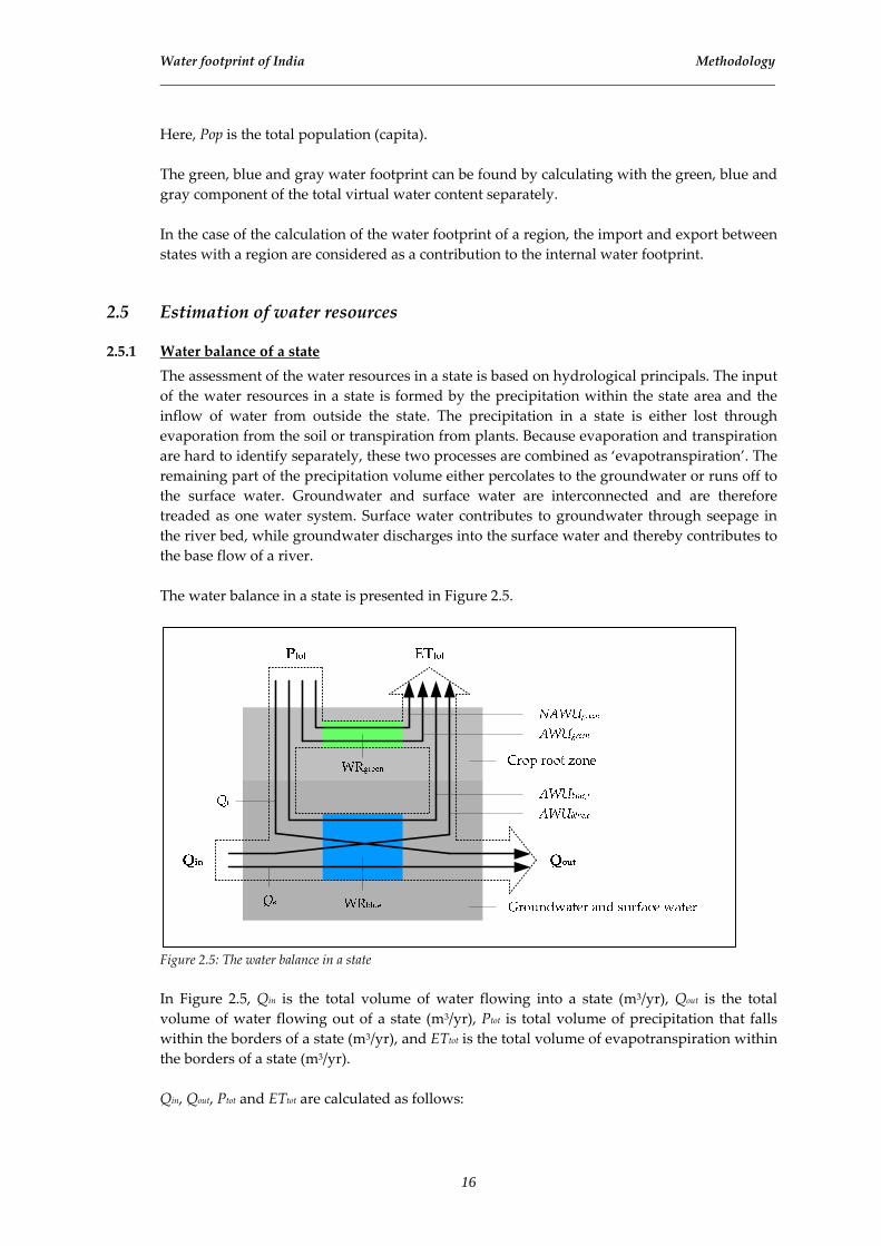
2.5.1 Water balance of a state The assessment of the water resources in a state is based on hydrological principals. The input of the water resources in a state is formed by the precipitation within the state area and the inflow of water from outside the state. The precipitation in a state is either lost through evaporation from the soil or transpiration from plants. Because evaporation and transpiration are hard to identify separately, these two processes are combined as ‘evapotranspiration’. The remaining part of the precipitation volume either percolates to the groundwater or runs off to the surface water. Groundwater and surface water are interconnected and are therefore treaded as one water system. Surface water contributes to groundwater through seepage in the river bed, while groundwater discharges into the surface water and thereby contributes to the base flow of a river. The water balance in a state is presented in Figure 2.5.
Figure 2.5: The water balance in a state In Figure 2.5, Qin is the total volume of water flowing into a state (m3/yr), Qout is the total volume of water flowing out of a state (m3/yr), Ptot is total volume of precipitation that falls within the borders of a state (m3/yr), and ETtot is the total volume of evapotranspiration within the borders of a state (m3/yr). Qin, Qout, Ptot and ETtot are calculated as follows:
16
Water footprint of India Methodology
[ ] [ ] [ ]sQsAWUsQ eebluein += , (55)
[ ] [ ] [sQsQsQ eiout += ] (56)
[ ] [ ] [ ] [ ] [ ]sAWUsNAWUsAWUsQsP ibluegreengreenitot ,+++= (57)
[ ] [ ] [ ] [ ] sAWUsAWUsNAWUsAWUsET eblueibluegreengreentot ,, [ ]+++= (58)
Here, AWUblue,e is the total use of external irrigation water (m3/yr), Qe is the outflow of external water from the state (m3/yr), Qi is the outflow of internal water from the state (m3/yr), AWUgreen is the total use of rainwater (m3/yr), NAWUgreen is the total use of rainwater in non agricultural areas (m3/yr), and AWUblue,i is the total use of internal irrigation water (m3/yr). As can be seen in Figure 2.5, a distinction is made between green water resources (WRgreen, m3/yr) and blue water resources (WRblue, m3/yr). The blue water resources can be further divided into an internal and an external component.
2.5.2 Internal water resources of a state Green water resources (WRgreen, m3/yr) are by definition internal water resources and are here defined as the total volume of vapour flows from the surface area in a state under rain fed conditions. The WRgreen are calculated as follows:
[ ] [ ] [ ]sNAWUsAWUsWR greengreengreen += (59)
The NAWUgreen are estimated as follows:
[ ] [ ] [ ]( ) [ ]sAsETsPMinsNAWU agricnoneffgreen ∗= 0, (60)
Here, Anonagric is the non agricultural area in a state (ha/yr). It is worth noticing that in this study, the non agricultural area, from which NAWUgreen is calculated, also represents the agricultural area that is not taken into account. The internal blue water resources (WRblue,i, m3/yr) capture the average annual flow in rivers and the recharge of groundwater generated from endogenous precipitation. The WRblue,i are calculated as follows:
[ ] [ ] [ ]sWRsPsWR greentotiblue −=, (61)
The total outflow of internal water from a state (Qi, m3/yr) is calculated as follows:
[ ] [ ] [ ]sAWUsWRsQ iblueibluei ,, −= (62)
Here, AWUblue,i is assessed as follows:
[ ] [ ] [ ] [ ]( )sWRsETsWRMinsAWU greentotiblueiblue −= ,,, (63)
In equation 63, the assumption is made that blue water use in a state originates as much as possible from internal water resources. The calculated AWUblue can now be separated into
17

Water footprint of India Methodology
AWUblue,i and AWUblue,e. This may lead to an underestimation of Qi and AWUblue,e and to an overestimation of Qe and AWUblue,i, while Qout remains the same. This also means that AWUblue,e only becomes larger than zero when Qi becomes zero, which is the case when the Qout is smaller than Qin.
2.5.3 External water resources of a state The external blue water resources of a state (WRblue,e, m3/yr) are defined as the total average annual flow in rivers and recharge of groundwater in a state that find their origin in other states or other countries. The assumption is made that the volume of groundwater that crosses state borders is negligible and is therefore omitted in this assessment. Furthermore the assumption is made that the transport of surface water between across state borders is only in the form of the larger rivers in India. The first step in the assessment of interstate river flows is the allocation of the river basin areas to the involved state areas. The total area of a state in a river basin (As,rb, km2) is calculated as follows:
[ ] [ ] [sArbArbsA srbrbs I=,, ] (64)
Here, As is the total area of a state (km2) and Arb is the total area of a river basin (km2). The part of the outflow of internal water resources of a state that contributes to the discharge volume of a river basin (Qi,rb, m3/yr) is calculated as follows:
[ ] [ ] [ ][ ]sA
sQrbsArbsQ
s
irbsrbi
∗=
,, ,
, (65)
The total outflow of water from a state in a river basin (Qout,rb, m3/yr) is now calculated as follows:
[ ] [ ] [ ]rbsQrbsQrbsQ rberbirbout ,,, ,,, += (66)
Here, Qe,rb is the part of the outflow of external water resources of a state that contributes to the discharge volume of river basin rb (m3/yr), which is calculated as follows:
[ ] [ ] [ ]sAWUrbsQrbsQ ebluerbinrbe ,,, ,, −= (67)
In Equation 67, Qin,rb is the inflow of external water resources into a state in a river basin (m3/yr), which is calculated as follows:
[ ] [∑=
=p
usrbirbin usrbsQrbsQ
1,, ,,, ] (68)
Here, us denotes a state upstream of state s, and p is the amount of states upstream of state s in river basin rb. The states upstream of state s in river basin rb are determined by the flow direction of the rivers through the states in river basin rb.
18
Water footprint of India Methodology
The WRblue,e of state s are now calculated as follows:
[ ] [ ]rbsQsWRk
rbrbineblue ,,, ∑= (69)
Here, k is the amount of river basins state s falls in. The total discharge volume of river basin rb (Qrb, m3/yr) is found as follows:
[ ] [ ]∑=
=n
soutrb rbsQrbQ
1
, (70)
Because of climatic variations within states, this calculation method might lead to an underestimate or overestimate of the discharge volume of the river basins. Unlike with the internal blue water resources, the external blue water resources of the states are interdependent on state scale. This means that the external water use in a state influences the external water availability downstream. The more states upstream of a state, the less accurate the calculated volume of external water resources is. Apart from this, the spatial variations are different for internal and external resources. For the internal resources the water availability is likely to be more spread over the state area, while the water availability from the external resources is limited to the area relatively close to the river flow. This assessment of water resources differs from other methods of assessing water resources. First of all, green water resources are taken into account. Second of all, in the assessment of internal renewable (blue) water resources, the withdrawal of irrigation water is taken into account.
2.6 Assessment of water scarcity
2.6.1 Water scarcity from production perspective Traditionally, water scarcity is seen from production perspective (WSprod, (‐)) by comparing water use to the available water resources in a state. This water scarcity is here divided into green water scarcity (WSprod,green, (‐)) and blue water scarcity (WSprod,blue, (‐)). The WSprod, WSprod,green and WSprod,blue are calculated as follows:
[ ] [ ] [ ] [ ][ ]sWR
sAWUsAWUsAWUsWS
tot
graybluegreenprod
++= (71)
[ ] [ ][ ]sWR
sAWUsWS
green
greengreenprod =, (72)
[ ] [ ] [ ][ ]sWR
sAWUsAWUsWS
blue
grayblueblueprod
+=, (73)
19
Water footprint of India Methodology
By definition the water scarcity from production perspective is between 0 and 1. Because of temporal and spatial dynamics in the water resources, not all water resources can be used and therefore water scarcity from production perspective will never reach 1. At which volume of water use the water becomes “scarce” is thus determined by the volume of utilizable water resources in a state.
2.6.2 Water scarcity from consumption perspective The green and blue water scarcity in a state can also be seen from consumption perspective (WScons, (‐)) by comparing the water footprint to the available water resources in a state. Also this water scarcity can be divided into green water scarcity (WScons,green, (‐)) and blue water scarcity (WScons,blue, (‐)). The WScons, WScons,green and WScons,blue are calculated as follows:
[ ] [ ] [ ] [ ][ ]sWR
sWFPsWFPsWFPsWS
tot
graygreenbluecons
++= (74)
[ ] [ ][ ]sWR
sWFPsWS
green
greengreencons =, (75)
[ ] [ ] [ ][ ]sWR
sWFPsWFPsWS
blue
dilutionbluebluecons
+=, (76)
In contrast to WSprod, the WScons can be more than 1. This is the case when more water is needed to produce the food for the inhabitants than is available in a state, which is the case in completely urban states like Delhi.
2.7 Calculation of water saving
2.7.1 Global water saving Water saving in a state is realised by a net import of a crop. The volume of water it would have taken to produce the imported amount of crop in the importing state itself is the water volume that is saved. The water saving in a state as a result of a net import of a crop (ΔSs, m3/yr) is calculated as follows:
[ ] [ ] [ ]( ) [ ] [ ]( )( ) [ scVWCscEscEscIscIscS insissinsisss ,,,,,, ,,,, ]∗+−+=Δ (77)
The global water saving as a result of interstate commodity trade (ΔSg, m3/yr) is calculated as follows:
[ ] [ ] [ ] [ ]( )eeiiieieg scVWCscVWCsscTsscS ,,,,,, −∗=Δ (78)
20

Water footprint of India Methodology
It can be seen that global water saving becomes negative (global water loss) when the VWC in the importing state is lower than the VWC in the exporting state. The total global water saving as a result of interstate commodity trade is found by summing up the global water savings of all interstate trade flows of a commodity. The global water saving as a result of interstate trade is divided into a blue, a green and a gray component. These components are found by calculating with blue, green and gray component of VWC separately.
2.7.2 Water saving and the theory of comparative advantage Based on equation 78, water is only globally saved when there is an absolute advantage in water productivity in the exporting state. This would mean that the export of crops from states with a natural absolute disadvantage in water productivity will never lead to global water saving. However, the economic theory of comparative advantage (Ricardo, 1817) shows how two states can both gain from crop trade if they specialize in the production of crops for which they have a comparative advantage and import the crops for which they have a comparative disadvantage. In the case of water productivity, this means that the absolute water saving that is realised by focussing on the relative advantage in water productivity is higher than the absolute water saving that is realised by focussing on the absolute advantage in water productivity (Wichelns, 2007). If we consider the states s1 and s2, which both produce the crops c1 and c2, next to the absolute advantages in water productivity, the relative advantage in water productivity can be determined. Equations 79 and 80 present the two possible situations.
[ ][ ]
[ ][ ]22
21
12
11
,,
,,
scWPscWP
scWPscWP
< (79)
[ ][ ]
[ ][ ]22
21
12
11
,,
,,
scWPscWP
scWPscWP
> (80)
In the first situation, state s1 has a comparative advantage in crop c1 and a comparative disadvantage in crop c2, while state s2 has a comparative advantage in crop c2 and a comparative disadvantage in crop c1. In the second situation, state s1 has a comparative advantage in crop c2 and a comparative disadvantage in crop c1, while state s2 has a comparative advantage in crop c1 and a comparative disadvantage in crop c2. State s1 should therefore specialize in crop c1 in the first situation and in crop c2 in the second situation, while state s2 should specialize in crop c2 in the first situation and in crop c1 in the second situation. These recommended specializations only depend on relative water productivities.
2.7.3 Relative water saving Apart from absolute water saving, there is also relative water saving. Relative water saving is realised by increasing the part of the vapour flow that contributes to the biomass of the crop
21
Water footprint of India Methodology
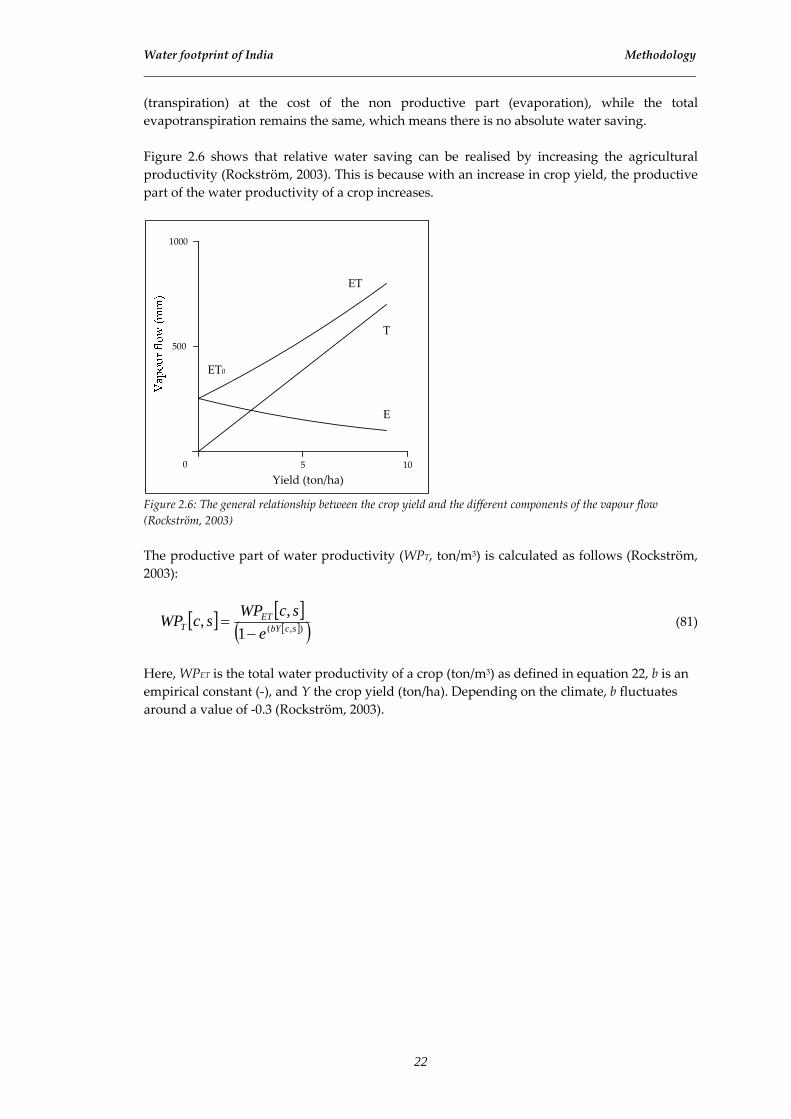
(transpiration) at the cost of the non productive part (evaporation), while the total evapotranspiration remains the same, which means there is no absolute water saving. Figure 2.6 shows that relative water saving can be realised by increasing the agricultural productivity (Rockström, 2003). This is because with an increase in crop yield, the productive part of the water productivity of a crop increases.
ET
T
E
ET0
Yield (ton/ha)
1000
500
0 5 10
Figure 2.6: The general relationship between the crop yield and the different components of the vapour flow (Rockström, 2003) The productive part of water productivity (WPT, ton/m3) is calculated as follows (Rockström, 2003):
[ ] [ ][ ]( )),(1,, scbY
ETT e
scWPscWP−
= (81)
Here, WPET is the total water productivity of a crop (ton/m3) as defined in equation 22, b is an empirical constant (‐), and Y the crop yield (ton/ha). Depending on the climate, b fluctuates around a value of ‐0.3 (Rockström, 2003).
22

3. Study scope and data collection
3.1 Study area India is located in South Asia bordering with Pakistan, China, Nepal, Bhutan, Myanmar and Bangladesh. In the north, along the border with China, India is situated in the Himalayan Range. Large rivers like the Indus, the Ganges and the Brahmaputra spring from this mountainous area. Below the Himalayan Range the Indo‐Gangetic Plain is found, which decreases from the west to the east. In the west, against the border with South Pakistan (Latitude 25°‐28°), the Thar Desert is situated. In the southern peninsular part of India the Deccan Plateau is found, with coastal hill regions (Western and Eastern Ghats). The southern part of India is surrounded by the Arabian Sea on the west side and the Bay of Bengal on the east side. Apart from the Thar Desert these geological features are all visible in the elevation map of India (Figure 3.1).
Figure 3.1: Elevation map of India (Source: en.wikipedia.org)
23

Water footprint of India Study scope and data collection
On a political scale India is divided into thirty‐six administrative divisions; twenty‐nine states, six union territories and the national capital territory Delhi (see Figure 3.2). The six union territories are Andaman & Nicobar Islands, Chandigarh (also the capital of both Punjab and Haryana), Dadra & Nagar Haveli, Daman & Diu, Lakshadweep Islands and Pondicherry. The states and the union territory of Pondicherry have an own local government. The remaining union territories are directly controlled by the national government, which is settled in Delhi.
Figure 3.2: Map of the Indian states & Union Territories (CDC, 2007) Approximately 70 % of the Indian population is currently living in rural areas (FAO, 2006a). This percentage is decreasing as a result of an increase in urbanisation in the past decades. In this study the following administrative divisions are excluded; Andaman & Nicobar Islands, Arunachal Pradesh, Chandigarh, Dadra & Nagar Haveli, Daman & Diu, Goa, Lakshadweep Islands, Manipur, Meghalaya, Mizoram, Nagaland, Sikkim and Tripura. These states and union territories are not taken into account, because they either have little area suitable for agriculture or have a small population (Appendix II). Therefore they are assumed to have no significant influence on the results of the study. Only in the assessment of the interstate trade, these areas are included to close the national crop balances. Another reason for the exclusion of these areas is that the precipitation is not well reported because of the small amount or even the absence of weather stations.
24

Water footprint of India Study scope and data collection
In November 2000, three states were split into two separate states; Uttaranchal was carved out of Uttar Pradesh, Jharkhand out of Bihar and Chhattisgarh out of Madhya Pradesh. Since this happened during the period on which this study is focused, it is worth noticing that data on the states involved prior November 2000 represent the combined performance of the split up states, which is separated by their relative individual performance after November 2000. Finally, the India can also be divided into four larger regions; northern, western, eastern and southern India. Northern India consists of Jammu & Kashmir, Himachal Pradesh, Punjab, Haryana, Uttaranchal, Uttar Pradesh and Delhi. Western India consists of Rajasthan, Gujarat, Madhya Pradesh and Maharashtra. Eastern India consists of Bihar, Jharkhand, West Bengal, Assam, Orissa and Chhattisgarh. And southern India consists of Karnataka, Andhra Pradesh, Kerala and Tamil Nadu. The total area considered in this study is 94% of the total territory of India and covers 98% of the population (Appendix II).
3.2 Crop coverage Not all crops that are grown in India can be taken into account in this study. Therefore a selection of crops is made. FAO distinguishes 176 primary crops in the FAOSTAT database (FAO, 2006a), of which 80 are produced in India in the period 1997‐2001 (Appendix III). These 80 crops can be summarized in 12 crop categories. The 12 crop categories and their total water use, production value and land use are given in Table 3.1.
1 Source: FAO (2006a), 2 Water use = production * Indian average virtual water content (source: Chapagain & Hoekstra, 2004), 3 Production value = production * producer price (US$ 1997‐2001, source: FAO, 2006a).
Table 3.1. Water use, production value and land use per crop category in the period 1997‐2001 Production1 Water use2 Production value3 Land use1
Crop categories 106 ton/yr 109 m3/yr % 109 US$/yr % 106 ha/yr %
Cereals 233 581 61 30 39 101 57
Oil crops 37 154 16 10 13 35 20
Pulses 13 58 6 5 6 21 12
Sugar crops 286 46 5 5 7 4 2
Fruits 45 39 4 11 14 4 2
Spices 2 17 2 2 2 3 1
Vegetables 68 16 2 9 11 5 3
Tree nuts 1 10 1 1 1 1 1
Stimulants 1 9 1 1 1 1 0
Starchy roots 30 7 1 3 4 2 1
Vegetable fibres 2 6 1 0 0 1 0
Other 1 6 1 1 1 1 0
Total 719 949 100 77 100 178 100
The water use of a crop is the production volume multiplied with the virtual water content of the crop (Chapagain & Hoekstra, 2004). The total crop water use in India is 949 billion m3/yr.
25
Water footprint of India Study scope and data collection
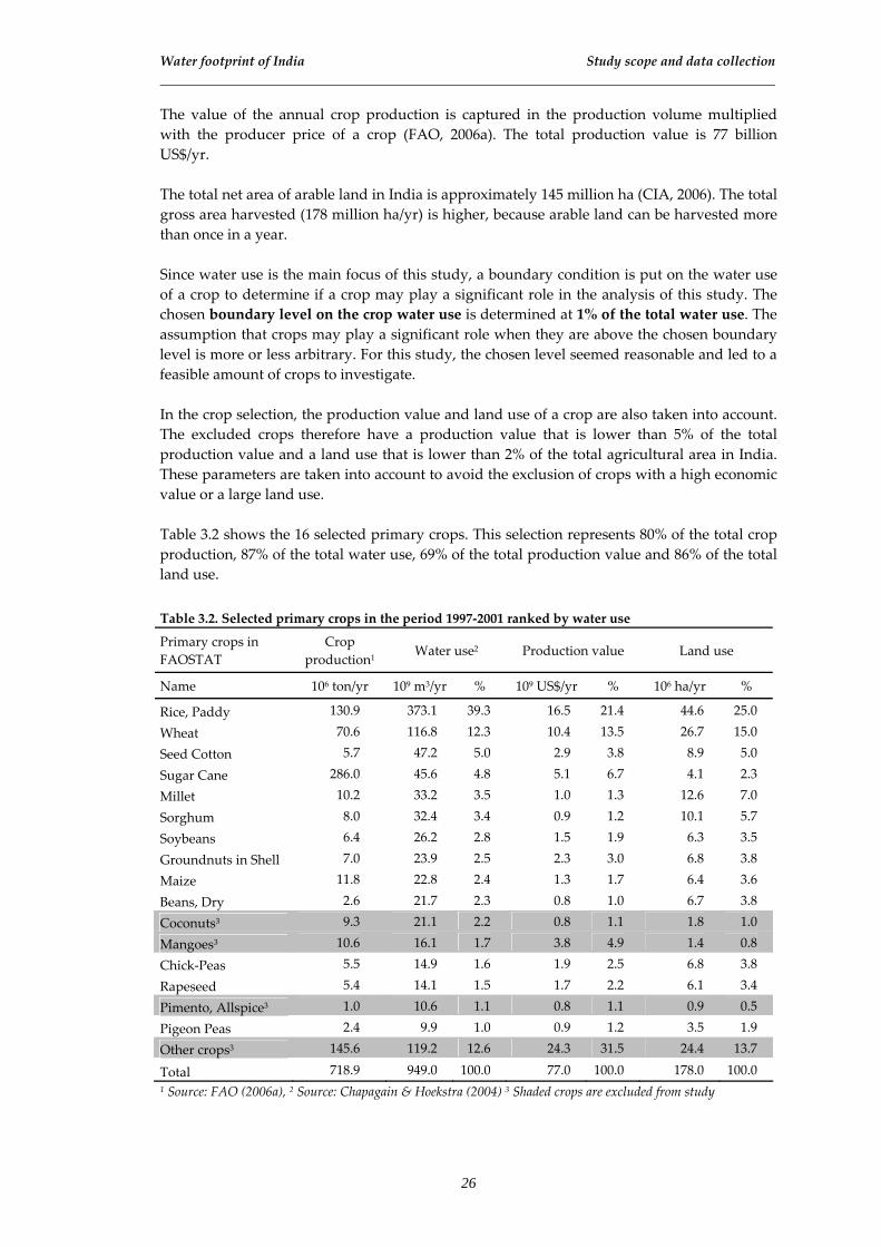
The value of the annual crop production is captured in the production volume multiplied with the producer price of a crop (FAO, 2006a). The total production value is 77 billion US$/yr. The total net area of arable land in India is approximately 145 million ha (CIA, 2006). The total gross area harvested (178 million ha/yr) is higher, because arable land can be harvested more than once in a year. Since water use is the main focus of this study, a boundary condition is put on the water use of a crop to determine if a crop may play a significant role in the analysis of this study. The chosen boundary level on the crop water use is determined at 1% of the total water use. The assumption that crops may play a significant role when they are above the chosen boundary level is more or less arbitrary. For this study, the chosen level seemed reasonable and led to a feasible amount of crops to investigate. In the crop selection, the production value and land use of a crop are also taken into account. The excluded crops therefore have a production value that is lower than 5% of the total production value and a land use that is lower than 2% of the total agricultural area in India. These parameters are taken into account to avoid the exclusion of crops with a high economic value or a large land use. Table 3.2 shows the 16 selected primary crops. This selection represents 80% of the total crop production, 87% of the total water use, 69% of the total production value and 86% of the total land use. Table 3.2. Selected primary crops in the period 1997‐2001 ranked by water use
Primary crops in FAOSTAT
Crop production1 Water use2 Production value Land use
Name 106 ton/yr 109 m3/yr % 109 US$/yr % 106 ha/yr %
Rice, Paddy 130.9 373.1 39.3 16.5 21.4 44.6 25.0
Wheat 70.6 116.8 12.3 10.4 13.5 26.7 15.0
Seed Cotton 5.7 47.2 5.0 2.9 3.8 8.9 5.0
Sugar Cane 286.0 45.6 4.8 5.1 6.7 4.1 2.3
Millet 10.2 33.2 3.5 1.0 1.3 12.6 7.0
Sorghum 8.0 32.4 3.4 0.9 1.2 10.1 5.7
Soybeans 6.4 26.2 2.8 1.5 1.9 6.3 3.5
Groundnuts in Shell 7.0 23.9 2.5 2.3 3.0 6.8 3.8
Maize 11.8 22.8 2.4 1.3 1.7 6.4 3.6
Beans, Dry 2.6 21.7 2.3 0.8 1.0 6.7 3.8
Coconuts3 9.3 21.1 2.2 0.8 1.1 1.8 1.0
Mangoes3 10.6 16.1 1.7 3.8 4.9 1.4 0.8
Chick‐Peas 5.5 14.9 1.6 1.9 2.5 6.8 3.8
Rapeseed 5.4 14.1 1.5 1.7 2.2 6.1 3.4
Pimento, Allspice3 1.0 10.6 1.1 0.8 1.1 0.9 0.5
Pigeon Peas 2.4 9.9 1.0 0.9 1.2 3.5 1.9
Other crops3 145.6 119.2 12.6 24.3 31.5 24.4 13.7
Total 718.9 949.0 100.0 77.0 100.0 178.0 100.0 1 Source: FAO (2006a), 2 Source: Chapagain & Hoekstra (2004) 3 Shaded crops are excluded from study
26
Water footprint of India Study scope and data collection
The primary crop “fresh vegetables not elsewhere specified” is omitted in table 3.2, although the production value is 5.3% of the national total. The reason for this is that this crop is already a leftover category within the category vegetables and therefore not suitable for further investigation, because data on individual crops are necessary to make an equal comparison between the states possible. At this point, it can be seen that not all crop categories from table 3.1 are well represented in the individual crop ranking in table 3.2. Based on these two tables the decision is made that the selected crops within the crop categories cereals, oil crops, pulses and sugar crops are further investigated in this study. This means that relatively important crops like mangoes and pimento are excluded. Furthermore coconut is excluded from this study, because of the lack of trade data on the processed products of this crop (like coir) and the lack of possible changes in the location of the crop production. According to this analysis, the selection of crops now represent 77% of the total crop production, 82% of the total water use, 61% of the total production value and 84% of the total land use. Finally, it is worth noticing that although rice is harvested as paddy rice, we only use the milled rice equivalent, which represents all the processed rice products interpolated to the equivalent of milled rice. Furthermore, it should be noted that all sugar originates from sugar cane in India and that the generic name dry beans in this study represents the crops mung bean, black gram and moth bean.
3.3 Data collection
3.3.1 Climatic parameters The data on the reference evapotranspiration (ET0) are calculated in CROPWAT (FAO, 2006b). In this program, the average ET0 is calculated per month with the FAO Penman‐Monteith method for 160 weather stations in India. Climatic data on these weather stations that are required as the input for this computation are taken from CLIMWAT (FAO, 2006c), which is the climatic database of CROPWAT. The available weather stations and the accompanying states are given in Appendix V. The average ET0 in a certain state for a certain month is found by taking the mean of the ET0 of all the weather stations situated in that state in that month. The amount of weather stations used per state varies from 1 in Himachal Pradesh and Delhi to 14 in Uttar Pradesh. In total 9 weather stations are excluded from the calculation of the average ET0, because they are either situated in non agricultural areas like deserts and mountains or very clearly cause an uneven distribution of the weather stations over the state area. The exclusion of these particular stations (Appendix IV) still does not guarantee that the calculated average ET0 is the “real” average ET0 of the state. In some states there are simple too few stations to present a reliable value for the entire state. The Ptot and Peff data for the 160 weather stations are again taken from CLIMWAT (FAO, 2006c) and the average Ptot and Peff per state is again found by taking the mean of the Ptot and Peff of all the weather stations situated in that state in that month. In the calculation of the virtual water contents, the same weather stations that are excluded in the calculation of the average ET0 per month per state are excluded here, because they are either situated in non agricultural areas like deserts and mountains or very clearly cause an uneven distribution of the weather stations over the state area. In the calculation of the internal and external blue water resources this might lead to a small underestimation in the case of the exclusion of rainy mountainous weather stations and to a small overestimation in the case of the exclusion of dry desert weather stations.
27

Water footprint of India Study scope and data collection
3.3.2 Crop parameters Data on the duration of the different growing stages, sowing and harvesting periods and crop coefficients are taken from Allen et al. (1998), Directorate of Rice Development (2006a) and Directorate of Pulses Development (2006a). Because of climatic differences and duration differences of crop varieties, the sowing and harvesting periods vary per region. To keep this study feasible a maximum of two sets of crop parameters are created for entire India; one for the wet season (kharif), which is roughly from June to December, and one for the dry season (rabi), which is roughly from December to April. For every crop the duration of these seasons is assessed, which is the same for all the Indian states. The generated parameters of the studied primary crops are presented in Appendix V.
3.3.3 Irrigated area fraction The data on the irrigated area fraction (iaf, (‐)) are taken from Directorate of Economics and Statistics (2003, 2004). The primary data are presented as the fraction of the total area of a crop under irrigation in a state during the agricultural years 1999‐2000 and 2000‐2001. The average iaf of these two agricultural years is taken as the total irrigated area fraction (iaftot(‐)). For the crops that are grown in one season, the iaf is equal to iaftot. For the crops that are grown in two seasons (kharif and rabi), the assumption is made that the iaf during rabi is as high as possible. The reason for this assumption is that the irrigation water is required the most during the dry season. The iaf during rabi and kharif is calculated as follows:
[ ] [ ]( )( )[ ]scA
iafscAscAMiniaf
rabi
tottotrabirabi ,
,,, ∗= (82)
[ ] [ ][ ]scA
iafscAiafscAiaf
kharif
rabirabitottotkharif ,
,, ∗−∗= (83)
Here, Arabi is the area of crop c in state s during rabi (ha/yr), Akharif is the area of crop c in state s during kharif (ha/yr) and Atot is the total area of crop c in state s (ha/yr). In the case of maize in Tamil Nadu, an exception is made for the calculation of the iaf during kharif and rabi. The reason for this is that in this special case, the irrigation water requirement as a percentage of the total water requirement is higher during kharif than during rabi. Therefore the iaf of maize in Tamil Nadu during the wet season is assumed to be as high as possible.
3.3.4 Dilution water requirement The data on the use of nitrate in fertilizers are taken from FAO (2005). FAO provides data on nitrate consumption (kg N/ha) for the most important crops in India in the agricultural year 2003‐2004 for irrigated and rain fed areas, in which no distinction is made between the states. The assumption is made that the values of the year 2003‐2004 also apply to the period 1997‐2001. Since the nitrate use is not given for all studied crops, the following assumptions are made: • The nitrate use on pearl millet is taken as the nitrate use on finger millet and small millets. • The nitrate use on pigeon peas is taken as the nitrate use on all pulses and soybean.
28

Water footprint of India Study scope and data collection
The total nitrate use for a crop (Nuse, kg N/ha) is now calculated as follows:
[ ] [ ] [ ] [ ]( ) [ ]scNsciafsciafscNscN rfauseiauseuse ,,1,,, ,, ∗−+∗= (84)
Here, Nuse,ia is the nitrate use on crop c in irrigated areas (kg N/ha), Nuse,rfa is the nitrate use on crop c in rain fed areas (kg/ha) and iaf is the irrigated area fraction (‐). The total nitrate use by states is taken from Directorate of Economics and Statistics (2003). These values are used for the comparison of the total gray water use in the different states as calculated in this study to the total gray water use in the different states as calculated from the total nitrate use. The leaching factor of nitrate is in this study determined at 0.10. This value is taken from Chapagain et al. (2006). The recommended level of nitrogen (N) in the groundwater is in this study taken to be 10 mg N/l (EPA, 2006; Chapagain et al., 2006), which corresponds with a nitrate (NO3ˉ) level of 44 mg/l (Agrawal, 1999). There are twelve states in India where nitrate levels are measured in the groundwater above the recommended level (Ministry of Water Resources, 2006a). The highest nitrate levels are found in Haryana and Punjab (Agrawal, 1999).
3.3.5 Product and value fractions of crops The product fractions of the crops for India are taken from FAO (2006a, 2006d) and are based on data from the period 1992‐1996. The assumption is made that these values are still accurate for our study period. The value fractions are taken from Chapagain & Hoekstra (2004). The product and value fractions of the studied crops used in this study are presented in Appendix VI.
3.3.6 Population The urban and rural population of the states are taken from Census of India (2006) and FAO (2006a). Census of India gives detailed data for the year 2001 for every state and FAO gives the total urban and rural population for the years 1997‐2001. The average population during the study period is found by combining the total number from FAO with the state distribution from Census of India. A map of the variation in the population density over the country and the total rural and urban population per state are presented in Appendix II. Data on the average income per state in the period 1997‐2001 is taken from Chandigarh Administration (2006).
3.3.7 National crop balance In the national crop balance, the domestic supply (production, import, export, stock change) and the domestic utilization (animal feed, seed, manufacturing, waste, uses and food) of a crop are determined for the study period 1997‐2001 (Appendix VII). In this study, the national balance of a crop is the average of the five annual crop balances, which are taken from the five annual food balance sheets of India (FAO, 2006a). In the cases when the primary crop is processed before consumption, the national balance is given for the primary crop and the processed crop. These annual crop balances are chosen as a base in this study, because no other balance includes other utilizations than human consumption.
29

Water footprint of India Study scope and data collection
In the national crop balance of sugar cane, the production, seed, feed, manufacture and food volumes for sugar cane for the years 1998 and 1999 have been adjusted to the production and utilization volumes of sugar cane as presented by the statistical database of the Indian Institute of Sugarcane Research (IISR, 2006). This is done because IISR are likely to present more reliable data. The national crop balance of the crop category pulses is only given for dry beans, dry peas and other pulses (FAO, 2006a). Since dry peas is not taken into account in this study and the utilizations of dry beans and other pulses are of the same percentage, the national balance is only assessed for pulses as a whole. Since there is no national balance for cotton lint, the assumption is made that all produced cotton lint that is not exported (FAO, 2006a), is used for local human consumption or exported to other states.
3.3.8 Crop area, production and yield The production data of cereals, oil crops and pulses are taken from Directorate of Economics and Statistics (2003, 2004), Directorate of Rice Development (2006b), Directorate of Wheat Development (2006), Directorate of Pulses Development (2006b) and FAORAP (2006). The production data of sugarcane are taken from the statistical database of the Indian Institute of Sugarcane Research (IISR, 2006). The production data of oil crops for the year 1997 is not available on state level and is therefore estimated on the total national production during 1997 and the relative state production volumes during the other years of the study period. The state production volumes are divided over the two main crop seasons in India: • kharif (wet monsoon season), which is approximately from June to November • rabi (dry winter season), which is approximately from November to April Besides these two main seasons, there are also crops grown during the summer season (also known as the pre‐kharif season), which is approximately from April to September, and thus overlaps the other two seasons. But since the crop production during this period is very low, this season is not taken into account in this study. The crop production during this season is either added to the crop production in the kharif season or to the crop production in the rabi season. The primary production data are presented in agricultural years, which are from July to June, while the data in the crop balances are presented in calendar years, which are from January to December (see Figure 3.3). Therefore, the production data from 1996‐1997 to 2000‐2001 are used for the rabi crops and the production data from 1997‐1998 to 2001‐2002 are used for the kharif crops. If a crop is grown in both seasons, the season with the largest crop production determines if the crop is here considered as a rabi crop or a kharif crop. This means that, for example, in the case of milled rice, kharif is considered as the main season, which means that the rabi production of calendar year 2002 is used and the rabi production of calendar year 1997 is excluded. In this step the following crops are considered as rabi crops; wheat, sugar cane, rapeseed and chickpeas. All other crops are here considered as kharif crops.
30

Water footprint of India Study scope and data collection
Figure 3.3: The overlap of calendar years and agricultural years
3.3.9 Crop consumption The data on the consumption of crops in the different states are all taken from reports of NSSO. This organisation carries out socio‐economic surveys throughout India on a regular basis. This means that the consumption of most commodities is estimated at least every five years. NSSO provides the state consumption per capita in rural and urban areas. For the crop category cereals, the consumption data for the years 1997‐2001 are taken from the NSSO (1998, 1999, 2001a, 2002, 2003). For the crop categories oil crops and sugar crops, the consumption data for the year 1999‐2000 are taken from NSSO (2001b). For the crop category pulses, the consumption data for the year 1999‐2000 are taken from NSSO (2001a). And for cotton lint, the consumption data for the year 2000‐2001 are taken from NSSO (2002). In the consumption data of oil crops, sugar crops and pulses some unrealistically high values are found for three north eastern states (Arunachal Pradesh, Manipur and Mizoram). For these states, the consumption data for year 1993‐1994 are taken from NSSO (1997). The total computed annual consumption per state (Cs,comp, ton/yr) is generated as follows:
[ ] [ ] [ ] urbanurbancapruralruralcapcomps PopscCPopscCscC ∗+∗= ,,, ,,, (85)
Here, Ccap,rural is consumption of a crop per capita in the rural area of a state (ton/cap/yr), Poprural is the rural population is a state (cap), Ccap,urban is consumption of a crop per capita in the urban area of a state (ton/cap/yr) and Popurban is the urban population in a state (cap). Next, the computed consumption volume of a state is interpolated to the consumption volume as given in the state crop balance (Cs, ton/yr), which is done to keep the national crop balance closed. The Cs is now calculated as follows:
[ ]
[ ] [ ]
[ ]∑=
⎟⎟⎠
⎞⎜⎜⎝
⎛
∗⎟⎟⎠
⎞⎜⎜⎝
⎛
=n
s
comps
tcomps
s
pfscC
cCpf
scC
scC
1
,
,
,
,
, (86)
Here, Ct is the consumption in the national crop balance (ton/yr) and pf the product fraction of the edible equivalent of crop c (‐). In general, the total computed crop consumption is a little lower than consumption as given in the national crop balance. But similarity between these two national crop consumption
31

Water footprint of India Study scope and data collection
volumes can be expected, because FAO regularly uses specific information on consumption trends from household surveys for benchmarking their estimates for subsequent years. According to FAO, the difference between the two numbers reflects “waste occurring between the retail level and the kitchen and losses of edible food and nutrients in the household, e.g., during storage, in preparation and cooking (which affect vitamins and minerals to a greater extent than calories, protein and fat), as plate‐waste, or as quantities fed to domestic animals and pets, or that thrown away”. Only in the case of chickpeas, non centrifugal and raw sugar, soybean and other edible oils, the computed consumption is significantly lower than the consumption as given in the national crop balance. The reason for this can be the exclusion of intermediate crop consumption in the NSSO method (NSSO, 2005). Intermediate consumption is here interpreted as the part of the crop that is used up in the process of further production (for example in factories or restaurants). The fact that there is a considerable volume of intermediate crop consumption in the case of crops involved is realistic. In the case of chickpeas, 60% is processed into a flour known as besan (Price et al., 2003), which is often mixed with flour from cereals. In the case of raw cane sugar, a large amount ends up in sweets, which are very popular in India, or other products. In the case of soybean and other edible oils, the soybean cake is processed into flour, which can again be mixed with flour from cereals, and a large part of the oil ends up in a mix of soybean oil and palm oil, which is known as vanaspati (Dohlman et al., 2003). In the special case of pigeon peas, the computed consumption is higher than the consumption in the national balance. This overestimation seems to indicate an error in the assessment of either FAO (2006a) or NSSO (2001a). Finally, it should be noted that the consumption data of cotton lint is presented as the average monthly expenditure on clothing per capita. Here, the assumption is made that the share of cotton lint in clothing is equal for all states. Since the consumption values are interpolated to the total value in the national balance, the unit of the consumption data does not form a problem.
3.3.10 Interstate trade For the crops that are processed before consumption, the surplus and interstate trade are calculated in the edible equivalent. The reason for this is that the processed crop may have a by‐product with a certain value that might be traded differently. An example of this is soybean which is processed into soybean oil and soybean cake. In these cases, the export, animal feed and primary crop consumption in the national balance of the primary crop are first transformed to the processed equivalent by the product fraction and then added to the crop utilizations in the national balance of the processed crop. In the case of pulses, the surplus of pulses is only calculated for pulses as a whole and the assumption is made that the interstate trade consists of chickpeas only. The reason for this is that, apart from the individual crop balances that are lacking, the computed consumption values of the individual pulses are too dodgy. The assumption is made that summing up the individual pulse consumption before the interpolation to the national balance eventually gives a better indication of total pulse consumption in a state than summing up after interpolating to the national balance. This assumption is based on the principle that individual pulses are exchangeable, which means that locally produced pulses are consumed before imported pulses. The interstate trade of pulses is caused by the interstate export of pulses from Madhya Pradesh, Maharashtra and Rajasthan. Based on the reported
32
Water footprint of India Study scope and data collection
consumption and production of the individual pulses in these three states (NSSO, 2001a, Directorate of Pulses, 2006b)), the assumption is made that the interstate trade of pulses exists of chickpeas only. In the case of edible oils, the surplus is calculated for groundnut oil, rapeseed oil and remaining edible oils and the assumption is made that the interstate trade of the remaining edible oils consists of soybean oil only. The reason for this is that, apart from the traditional Indian edible oils groundnut oil and rapeseed oil, the computed consumption values of the edible oils are heavily underestimated. For the remaining edible oils (soybean oil and cottonseed oil), the same assumption is made as for pulses. The surplus of this group is therefore calculated for the remaining edible oils as a whole. In the calculation of surplus of remaining edible oils, sunflower seed oil, coconut oil and palm oil are included. These oils are included in this step, to prevent an oblique situation in the final surplus of the remaining edible oils in the Indian states. The interstate trade of the remaining edible oils is now only caused by the interstate export from Madhya Pradesh. Based on the consumption of edible oils in this state (NSSO, 2001b) and the production of soybean, the assumption is made that the interstate trade of the remaining edible oils exists of soybean only. In line with the rest of the study this would mean that Madhya Pradesh is the only state that uses the crop for other utilizations that human consumption, seed use and waste. Since the coverage of all national utilizations of all remaining edible oils would create a deficit of remaining edible oils in Madhya Pradesh, the remaining utilizations of the primary crops are in this case taken as a fixed percentage of the production (like the assessment of the seed use and waste of a crop) and the import goes to the stock increase (this is because it is unclear where the imported oils are consumed). Madhya Pradesh now only has to cover the stock increase and export of soybean.
3.3.11 Water resources In this study, the water resources of the Indian states are not calculated from existing estimates on the water resources in India. Still a few studies on the water resources of India are analysed as a rough check for the calculated water resources in this study. These estimates on the water resources of India (Chaturvedi, 1985; FAO, 2003, 2006e; Ministry of Water Resources, 2006b) are presented in Appendix XVI. From the previous estimates of the water resources in India, the conclusion can be made that precipitation estimates range from 3559 to 4000 km3 (1083 to 1194 mm), blue water resources estimates range from 1272 to 1650 km3 and green water resources estimates range from 2287 to 2350 km3. Because precipitation is the single input of the calculation of the internal water resources, it determines a large part of the outcome of the internal blue and green water resources. Especially the blue water resources seem to be sensitive to change in precipitation. The green water resources seem to be less sensitive to change in precipitation. A map of the average annual precipitation, taken from India Meteorological Department (IMD, 2006), is shown in Appendix XVII. As can be seen in Appendix XVII, there is an enormous spatial and temporal variation in the precipitation in India; the north eastern part and the Western Ghats receive considerably more rainfall than the central part of the Deccan plateau and most parts of north western India. The two spatial extremes are the north eastern state Meghalaya, where the hill station Cherrapunji receives the most rainfall in the world (11420 mm), and the Rajasthan desert, where some of the driest places on earth can be found. Furthermore, India receives around 75% of its annual precipitation during the monsoons. Nearly all Indian states receive most of their rainfall during the south west monsoon which takes place in India from June to the end of September.
33
Water footprint of India Study scope and data collection
Only Tamil Nadu receives most of its rainfall during the north east monsoon which takes place in India from October to December. Since precipitation is of large importance for the outcome of the estimates on water resources, rainfall data are taken from IITM (2006), which collected rainfall data for India from the year 1871 and onwards. In these data four Himalayan states are excluded; Jammu & Kashmir, Himachal Pradesh, Uttaranchal and Arunachal Pradesh. These data lead to an average annual precipitation of 1088 mm. In the calculation of the external blue water resources, the data on state areas situated in river basins and the direction of rivers through the Indian states (Appendix XIX) are taken from Ministry of Water Resources (2006c). The total annual inflow of water from other countries (China, Nepal and Bhutan) is taken to be 636 km3 (FAO, 2006e). This estimate is for a large part based on one rough number (347 km3) of the Chinese government, which represents the inflow from China to Jammu & Kashmir (Indus river basin) and Arunachal Pradesh (Brahmaputra river basin). Based on data of the weather stations in Jammu & Kashmir, it seems that the eastern part of this state, where the Indus enters the country, receives very little rainfall. It is worth noticing that the highest Himalayan Range which is in India situated in the states of Himachal Pradesh and Uttaranchal seems to act as a precipitation barrier. This conclusion is based on data from weather stations in the involved states and the annual rainfall map of India. The assumption is made that the precipitation in the far western part of Tibet, where the Indus springs from, is of the same magnitude as in the eastern part of Jammu & Kashmir. This assumption lead to the estimate that 20 km3 of water annually enters India through the Indus river basin (10 km3 in the Indus and 10 km3 in the Satluj tributary). This estimate means that a volume 327 km3 of water flows from China to India through the Brahmaputra basin. The inflow from Nepal and Bhutan is estimated at 210 km3 and 90 km3 (FAO, 2006e). The inflow from Nepal enters India in the states Uttar Pradesh and Bihar and is thereby part of the Ganges river basin. FAO estimates that the distribution is 80 km3 to Uttar Pradesh and 130 km3 to Bihar. The inflow from Bhutan contributes entirely to the Brahmaputra basin though the states West Bengal and Assam. In this study the assumption is made that the distribution is 15 km3 to West Bengal and 75 km3 to Assam, which is based on the percentage of the total area of Bhutan that contribute to the two Indian states.
34

4. Virtual water content of crops
4.1 Virtual water content of the primary crops The blue, green, gray and total virtual water content of the primary crops is tabulated by state in Appendix VIII. The virtual water content of crops that are grown during kharif (wet season) as well as rabi (dry season), is presented for kharif, rabi and the total of both seasons, which is the average of both seasons weighted by the seasonal production in a state. In general, the virtual water content of the crops is relatively lower in the northern and southern states and relatively higher in the western and eastern states. This variation in virtual water contents is largely determined by the difference in crop yield. This difference is mainly caused by the difference in development of the agricultural areas, which can be expressed in the form of a high or low fraction of irrigated area and a high or low fertilizer use. Another reason for a variation in the virtual water content of a crop is the difference in climate. In general, the influence of climate on the magnitude of the virtual water content is not very high. On one hand, a higher evapotranspiration rate leads to a higher crop water requirement and therefore to a higher crop water use, but on the other hand, a higher evapotranspiration rate leads to a higher biomass of the crop, which leads to a higher yield. However, with a lower crop yield, the non productive part of the evapotranspiration rate (the part that does not contribute to the biomass of the crop) is relatively higher and therefore the influence of the climate on the virtual water content is relatively higher. The blue, green and gray component of the total water use is given by crop in Figure 4.1.
0
50
100
150
200
250
300
350
Milledrice
Wheat Coarsecereals
Sugarcane
Pulses Oil crops Seedcotton
Water use (billion m3/yr)
Gray
GreenBlue
Figure 4.1: The blue, green and gray volume of water used in India for crop production in the period 1997‐2001.
35
Water footprint of India Virtual water contents of crops
The total volume of water used in India for the production of the studied primary crops is 792 billion m3/yr. The total blue water use is 219 billion m3/yr, the total green water use 479 billion m3/yr and the total gray water use billion 95 m3/yr. Figure 4.1 shows that the production of milled rice is responsible for a water use of 348 billion m3/yr, which is 44% of the total water use, and that the production of wheat uses a water volume of 100 billion m3/yr, which is 13% of the total water use. Furthermore Figure 4.1 shows that the water use in case of milled rice consists mainly (67%) of green water and that the water use in case of wheat consists mainly (58%) of blue water. According to Directorate of Economics and Statistics (2003), the average nitrate use in India during the study period is 11.2 billion kg N/yr. Applying the leaching factor of 10% and a recommended level of 10 mg N/l, this translates in a total gray water use of 112 billion m3/yr for the dilution of the total nitrate consumption in the Indian agriculture. This means that 85% of the total gray water use is represented in this study. Since this gray water use is based on the average nitrate use for crops in whole India, the calculated gray water use is compared to the total nitrate consumption per state (Directorate of Economics and Statistics, 2003). This comparison shows that the gray water use in Andhra Pradesh, Karnataka and Punjab is underestimated in this study and that the gray water use is Madhya Pradesh, Chhattisgarh, Orissa and Rajasthan is overestimated (Appendix IX). In this study, the crops grown in the dry season (rabi) in non irrigated areas receive too little water during the growth period, which results in an underestimation of the virtual water content of a crop (Appendix VIII). The first reason for this underestimation of crop water use is the fact that a crop might be grown in a part of a state which receives more precipitation than the state average precipitation, which is used in this study. An example of this is the growth of soybean in Rajasthan under rain fed conditions, which takes place in the relatively wet south eastern part of the state. Another reason might be an incorrect assessment of the growth periods of the crops in the different states, which are in this study taken to be the same for all states. A third reason can be the fact that there might still be green water available in the soil after the monsoon, which is not taken into account in this study.
4.2 Virtual water content of milled rice Because milled rice is the crop with the largest contribution to the water use in India, the virtual water content of milled rice is described here with more detail. The virtual water content of milled rice varies from 2914 m3/ton in Punjab to 8142 m3/ton in Madhya Pradesh, with a national average of 4073 m3/ton. The wide range in the virtual water content of milled rice in India is mainly caused by differences in crop yield, which has a large correlation with the fraction of the crop area under irrigation (Appendix X). The yield of milled rice grown under rain fed conditions is considerably lower than the yield of milled rice grown under irrigated conditions, which is caused by a higher potential yield of the variety that is grown under irrigation, which requires a high level of irrigation and a high fertilizer use (Directorate of Rice Development, 2006c). The variation of the virtual water content of milled rice over the Indian states is shown in Figure 4.2.
36

Water footprint of India Virtual water contents of crops
VWC (m3/ton)< 35003500 - 45004500 - 55005500 - 6500> 6500 no value
Figure 4.2: The total virtual water content of milled rice in the Indian states during the period 1997‐2001. Comparable states like Punjab and Haryana have a significant difference in the virtual water content of milled rice, because in this study no distinction is made between basmati rice and non basmati rice in the irrigated areas in North India. Basmati rice, only grown in North India, requires relatively more water than non basmati rice (Directorate of Rice Development, 2006a, 2006b) and the fraction basmati rice to the total rice production is considerably larger in Haryana than in Punjab. Finally, it is worth noticing that milled rice is grown during two seasons in East India. In the dry season the yields are relatively higher, because milled rice is grown under irrigation in this season. With this extra season, the total virtual water content is reduced a little in the eastern states.
4.3 Comparison with other studies The average virtual water content for whole India as calculated in this study (Appendix VIII) and as calculated by Chapagain & Hoekstra (2004) are presented for the studied crops in Table 4.1. It should be noted that the values as calculated by Chapagain & Hoekstra do not include the gray component of the virtual water content and should therefore be compared with the sum of the blue and the green component as calculated in this study.
37

Water footprint of India Virtual water contents of crops
Table 4.1: Average virtual water content for the studied primary crops in India1
Virtual water content Crop Season
Blue Green Gray Total Chapagain & Hoekstra2
Unit m3/ton Year 1997‐2001
Kharif 775 3086 430 4290 ‐ Rabi 2093 330 344 2767 ‐
Milled rice
Total 963 2692 417 4073 4113 Wheat Rabi 822 214 376 1412 1654
Kharif 75 2281 231 2587 ‐ Rabi 780 351 210 1342 ‐
Maize
Total 182 1989 228 2399 1937 Millet Kharif 56 3892 273 4222 3269
Kharif 27 4163 282 4473 ‐ Rabi 690 1149 496 2335 ‐
Sorghum
Total 301 2918 370 3589 4053 Sugar cane Rabi 126 91 18 234 159 Chickpeas Rabi 1159 598 314 2071 2712 Pigeon peas Kharif 127 5497 297 5922 4066
Kharif 233 8597 662 9492 ‐ Rabi 533 1484 445 2463 ‐
Dry beans
Total 313 6706 604 7623 8335 Soybean Kharif 23 3308 196 3526 4124
Kharif 95 4356 243 4694 ‐ Rabi 2715 381 218 3315 ‐
Groundnut in shell
Total 705 3430 237 4372 3420 Rapeseed Rabi 2553 635 785 3972 2618 Seed cotton Kharif 1887 7300 1446 10633 8264 1 Source: Appendix VIII, 2 Total virtual water content as calculated by Chapagain & Hoekstra (2004). From our current study results, the conclusion can be made that in the case of some crops, there is a significant difference between the values as calculated by Chapagain & Hoekstra and values as calculated in this study. It is interesting to know what assumptions in both studies caused this difference. The following general conclusions on the differences between the two studies can be made: • Chapagain & Hoekstra use only one set of monthly values of ET0 for entire India. For the
crops that are not grown all over India, this leads to different values. Wheat for example is mostly grown in northern India, where it can get relatively cold in the dry winter season. Therefore the average crop water requirement of wheat in India is determined at 304 mm in this study against 438 mm in the study of Chapagain & Hoekstra.
• For some crops other growth periods are used in this study, which leads to a different ETc. • Chapagain & Hoekstra assume the irrigated area is 100%, while in fact this is not the case,
because a significant part of the crops grown in India are rain fed. This leads to lower values of the water use in this study.
• Chapagain & Hoekstra add extra water to the crop water requirement of milled rice to compensate for the high level of percolation. In this study this is not done, since percolated water does not leave the water system and is therefore not considered as lost.
Furthermore, the blue water use as calculated in this study can be compared with a study on irrigation water use (Rosegrant et al., 2002), in which the irrigation water consumption in India in 1995 is estimated at 321 billion m3/yr. This is 47% higher than the value calculated in this study. Two possible reasons for this significant difference can be the exclusion of irrigation water losses in this study and the exclusion of approximately 20% of the crops.
38
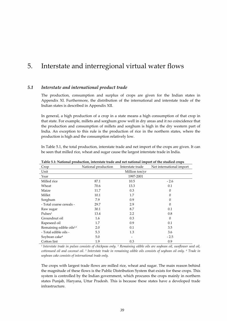
5. Interstate and interregional virtual water flows
5.1 Interstate and international product trade The production, consumption and surplus of crops are given for the Indian states in Appendix XI. Furthermore, the distribution of the international and interstate trade of the Indian states is described in Appendix XII. In general, a high production of a crop in a state means a high consumption of that crop in that state. For example, millets and sorghum grow well in dry areas and it no coincidence that the production and consumption of millets and sorghum is high in the dry western part of India. An exception to this rule is the production of rice in the northern states, where the production is high and the consumption relatively low. In Table 5.1, the total production, interstate trade and net import of the crops are given. It can be seen that milled rice, wheat and sugar cause the largest interstate trade in India. Table 5.1: National production, interstate trade and net national import of the studied crops Crop National production Interstate trade Net international import Unit Million ton/yr Year 1997‐2001 Milled rice 87.1 10.5 ‐ 2.6 Wheat 70.6 13.3 0.1 Maize 11.7 0.3 0 Millet 10.1 1.7 0 Sorghum 7.9 0.9 0 ‐ Total coarse cereals ‐ 29.7 2.9 0 Raw sugar 30.1 8.7 0.1 Pulses1 13.4 2.2 0.8 Groundnut oil 1.6 0.3 0 Rapeseed oil 1.7 0.9 0.1 Remaining edible oils2,3 2.0 0.1 3.5 ‐ Total edible oils ‐ 5.3 1.3 3.6 Soybean cake4 5.0 ‐ ‐ 2.5 Cotton lint 1.9 0.3 0.9 1 Interstate trade in pulses consists of chickpeas only. 2 Remaining edible oils are soybean oil, sunflower seed oil, cottonseed oil and coconut oil. 3 Interstate trade in remaining edible oils consists of soybean oil only. 4 Trade in soybean cake consists of international trade only. The crops with largest trade flows are milled rice, wheat and sugar. The main reason behind the magnitude of these flows is the Public Distribution System that exists for these crops. This system is controlled by the Indian government, which procures the crops mainly in northern states Punjab, Haryana, Uttar Pradesh. This is because these states have a developed trade infrastructure.
39

Water footprint of India Interstate and interregional virtual water flows
The largest interstate trade flows are created by the interstate trade in milled rice and wheat from Punjab to Bihar, Kerala and Maharashtra and from Uttar Pradesh to Bihar and Jharkhand (Appendix XII). The largest international trade flows are caused by the export of soybean cake (from Madhya Pradesh) to South East Asia, the export of milled rice, and the international import of palm oil from Indonesia and Malaysia (FAO, 2006a).
5.2 Interstate virtual water flows The net virtual water flows between the states are presented in Appendix XIII. The total interstate and international virtual water import and export from and to the Indian states together the net virtual water import is given in Table 5.2. Table 5.2: Water use, virtual water flows and net import by state
Virtual water export Virtual water import States
Water use Interstate International Interstate International1
Net VW import
Unit 106 m3/yr Year 1997‐2001 Andhra Pradesh 66652 4952 1711 569 774 ‐5319 Assam 17812 4 0 2304 155 2455 Bihar 38283 149 1 14469 983 15302 Chhattisgarh 27912 2835 699 2544 558 ‐431 Delhi 267 0 0 4026 683 4709 Gujarat 42678 3847 3120 9186 941 3160 Haryana 31956 13006 2105 638 339 ‐14134 Himachal Pradesh 2439 26 0 1439 212 1626 Jammu & Kashmir 4143 26 0 3101 178 3254 Jharkhand 11593 0 0 8853 430 9283 Karnataka 43358 3130 365 3699 214 418 Kerala 2897 0 2 10180 891 11069 Madhya Pradesh 64863 7671 8254 4933 162 ‐10831 Maharashtra 80390 5788 3949 11836 1461 3560 Orissa 37801 149 21 4552 416 4797 Punjab 43036 19351 4095 1658 914 ‐20874 Rajasthan 60169 9852 388 5504 512 ‐4224 Tamil Nadu 35496 4293 285 1397 967 ‐2214 Uttar Pradesh 127855 24542 2988 4777 1953 ‐20800 Uttaranchal 5581 1447 126 960 164 ‐449 West Bengal 47141 4447 1094 6238 749 1445 Total 792321 105516 29203 105516 13953 ‐15250 1 National import is blue and green water only (Chapagain & Hoekstra, 2004). Since no distinction is made between green and blue by Chapagain & Hoekstra, the total international virtual water import is contributed entirely to the blue external water footprint. The total virtual water flow as a result of interstate crop trade in India is 106 billion m3/yr. This is 13% of the total water use. The export of virtual water is 29 billion m3/yr (4% of the total water use) and the import of virtual water is 14 billion m3/yr, which results in a net export of 15 billion m3/yr. So in total 17% of the total volume of water used for crop production in India is exported to other states or countries.
40
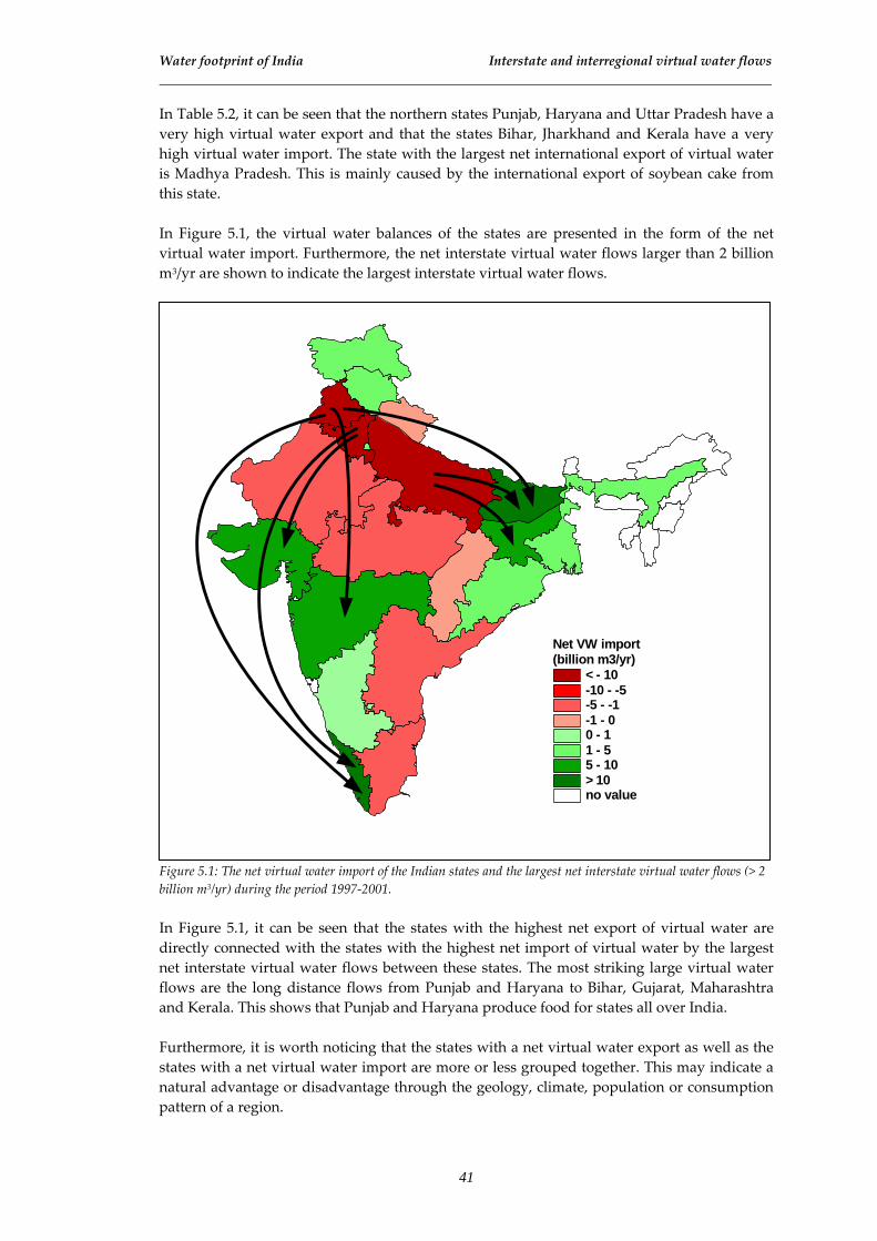
Water footprint of India Interstate and interregional virtual water flows
In Table 5.2, it can be seen that the northern states Punjab, Haryana and Uttar Pradesh have a very high virtual water export and that the states Bihar, Jharkhand and Kerala have a very high virtual water import. The state with the largest net international export of virtual water is Madhya Pradesh. This is mainly caused by the international export of soybean cake from this state. In Figure 5.1, the virtual water balances of the states are presented in the form of the net virtual water import. Furthermore, the net interstate virtual water flows larger than 2 billion m3/yr are shown to indicate the largest interstate virtual water flows.
Net VW import(billion m3/yr)
< - 10-10 - -5-5 - -1-1 - 00 - 11 - 55 - 10> 10no value
Figure 5.1: The net virtual water import of the Indian states and the largest net interstate virtual water flows (> 2 billion m3/yr) during the period 1997‐2001. In Figure 5.1, it can be seen that the states with the highest net export of virtual water are directly connected with the states with the highest net import of virtual water by the largest net interstate virtual water flows between these states. The most striking large virtual water flows are the long distance flows from Punjab and Haryana to Bihar, Gujarat, Maharashtra and Kerala. This shows that Punjab and Haryana produce food for states all over India. Furthermore, it is worth noticing that the states with a net virtual water export as well as the states with a net virtual water import are more or less grouped together. This may indicate a natural advantage or disadvantage through the geology, climate, population or consumption pattern of a region.
41
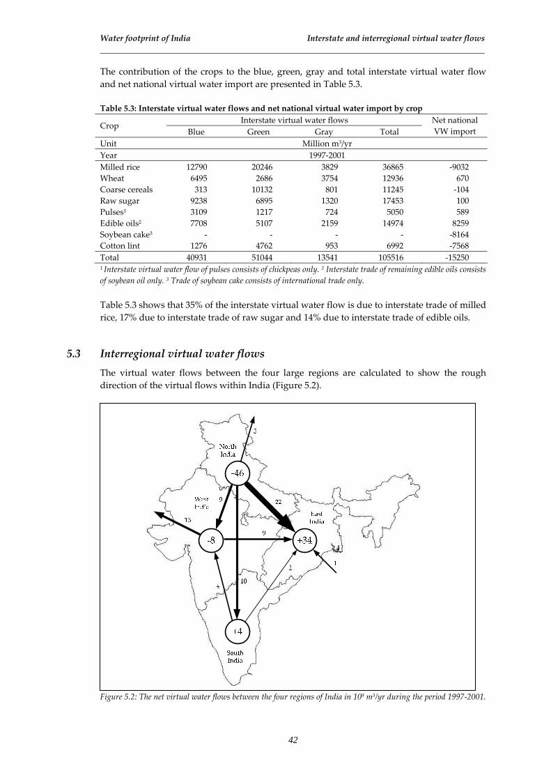
Water footprint of India Interstate and interregional virtual water flows
The contribution of the crops to the blue, green, gray and total interstate virtual water flow and net national virtual water import are presented in Table 5.3. Table 5.3: Interstate virtual water flows and net national virtual water import by crop
Interstate virtual water flows Crop
Blue Green Gray Total Net national VW import
Unit Million m3/yr Year 1997‐2001 Milled rice 12790 20246 3829 36865 ‐9032 Wheat 6495 2686 3754 12936 670 Coarse cereals 313 10132 801 11245 ‐104 Raw sugar 9238 6895 1320 17453 100 Pulses1 3109 1217 724 5050 589 Edible oils2 7708 5107 2159 14974 8259 Soybean cake3 ‐ ‐ ‐ ‐ ‐8164 Cotton lint 1276 4762 953 6992 ‐7568 Total 40931 51044 13541 105516 ‐15250 1 Interstate virtual water flow of pulses consists of chickpeas only. 2 Interstate trade of remaining edible oils consists of soybean oil only. 3 Trade of soybean cake consists of international trade only. Table 5.3 shows that 35% of the interstate virtual water flow is due to interstate trade of milled rice, 17% due to interstate trade of raw sugar and 14% due to interstate trade of edible oils.
5.3 Interregional virtual water flows The virtual water flows between the four large regions are calculated to show the rough direction of the virtual flows within India (Figure 5.2).
Figure 5.2: The net virtual water flows between the four regions of India in 109 m3/yr during the period 1997‐2001.
42

Water footprint of India Interstate and interregional virtual water flows
Figure 5.2 shows that the largest interregional virtual water flow is from North India to East India. This virtual water flow has a volume of 22 billion m3/yr and consists for 54% of rice, for 21% of raw sugar and for 18% of wheat. Furthermore, this total water volume of 22 billion m3/yr consists for 38% of blue water, 48% of green water and for 14% of gray water. The interregional virtual water flow from North to East India originates for 66% from Uttar Pradesh, 19% from Punjab and 13% from Haryana and is destined for 52% for Bihar, 29% for Jharkhand and 14% for West Bengal. Table 5.2 and Figure 5.2 show a total net international export of virtual water of 15 billion m3/yr. This shows a relatively good resemblance with the study of Chapagain & Hoekstra (2004), in which the net international export of virtual water is determined at 18 billion m3/yr.
43

44
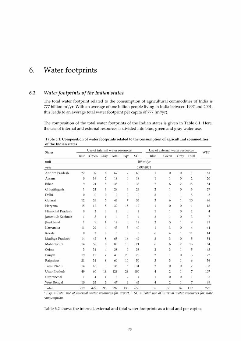
6. Water footprints
6.1 Water footprints of the Indian states The total water footprint related to the consumption of agricultural commodities of India is 777 billion m3/yr. With an average of one billion people living in India between 1997 and 2001, this leads to an average total water footprint per capita of 777 (m3/yr). The composition of the total water footprints of the Indian states is given in Table 6.1. Here, the use of internal and external resources is divided into blue, green and gray water use. Table 6.1: Composition of water footprints related to the consumption of agricultural commodities of the Indian states
Use of internal water resources Use of external water resources States Blue Green Gray Total Exp1 SC2 Blue Green Gray Total
WFP
unit 109 m3/yr
year 1997‐2001
Andhra Pradesh 22 39 6 67 7 60 1 0 0 1 61
Assam 0 16 2 18 0 18 1 1 0 2 20
Bihar 9 24 5 38 0 38 7 6 2 15 54
Chhattisgarh 1 24 3 28 4 24 2 1 0 3 27
Delhi 0 0 0 0 0 0 3 1 1 5 5
Gujarat 12 26 5 43 7 36 3 6 1 10 46
Haryana 15 12 5 32 15 17 1 0 0 1 18
Himachal Pradesh 0 2 0 2 0 2 1 1 0 2 4
Jammu & Kashmir 1 3 1 4 0 4 2 1 0 3 7
Jharkhand 1 9 1 12 0 12 3 5 1 9 21
Karnataka 11 29 4 43 3 40 1 3 0 4 44
Kerala 0 2 0 3 0 3 6 4 1 11 14
Madhya Pradesh 14 42 8 65 16 49 2 3 0 5 54
Maharashtra 14 58 8 80 10 71 6 6 2 13 84
Orissa 3 31 4 38 0 38 2 3 1 5 43
Punjab 19 17 7 43 23 20 2 1 0 3 22
Rajasthan 21 31 8 60 10 50 3 3 1 6 56
Tamil Nadu 14 18 3 35 5 31 2 0 0 2 33
Uttar Pradesh 49 60 18 128 28 100 4 2 1 7 107
Uttaranchal 1 4 1 6 2 4 1 0 0 1 5
West Bengal 10 32 5 47 6 42 4 2 1 7 49
Total 219 479 95 792 135 658 55 51 14 119 7771 Exp = Total use of internal water resources for export, 2 SC = Total use of internal water resources for state consumption. Table 6.2 shows the internal, external and total water footprints as a total and per capita.
45
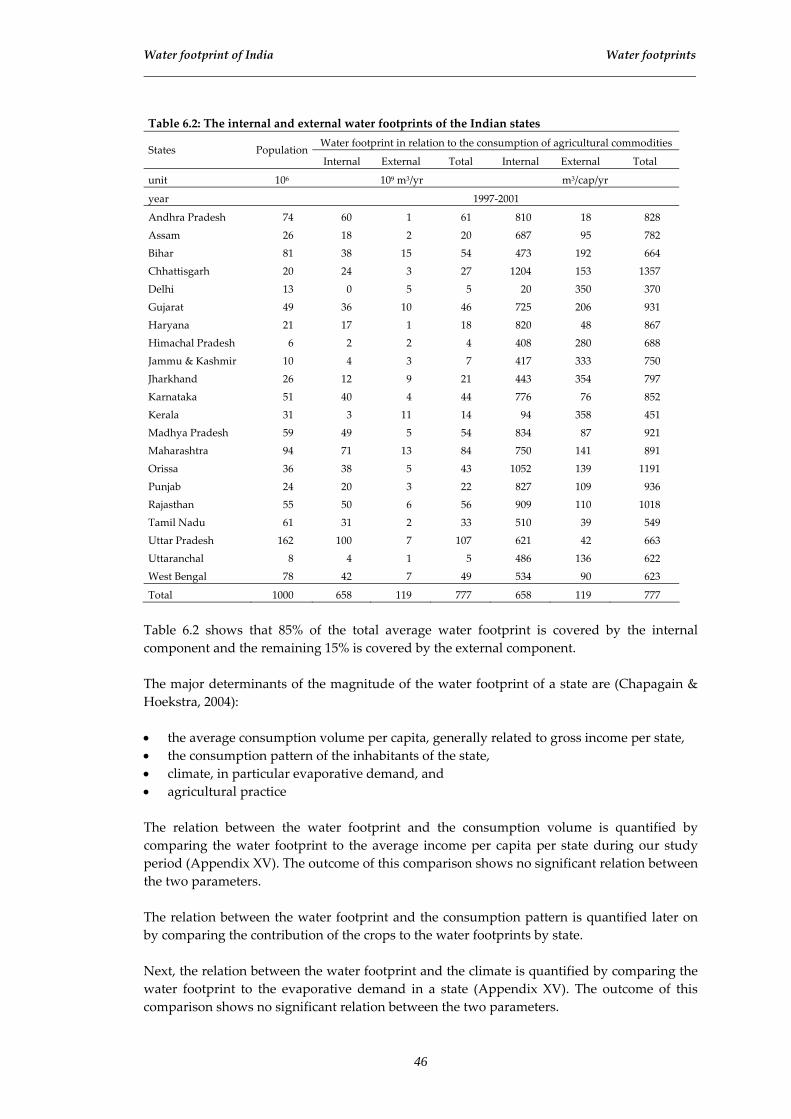
Water footprint of India Water footprints
Table 6.2: The internal and external water footprints of the Indian states
Water footprint in relation to the consumption of agricultural commodities States Population
Internal External Total Internal External Total
unit 106 109 m3/yr m3/cap/yr
year 1997‐2001
Andhra Pradesh 74 60 1 61 810 18 828
Assam 26 18 2 20 687 95 782
Bihar 81 38 15 54 473 192 664
Chhattisgarh 20 24 3 27 1204 153 1357
Delhi 13 0 5 5 20 350 370
Gujarat 49 36 10 46 725 206 931
Haryana 21 17 1 18 820 48 867
Himachal Pradesh 6 2 2 4 408 280 688
Jammu & Kashmir 10 4 3 7 417 333 750
Jharkhand 26 12 9 21 443 354 797
Karnataka 51 40 4 44 776 76 852
Kerala 31 3 11 14 94 358 451
Madhya Pradesh 59 49 5 54 834 87 921
Maharashtra 94 71 13 84 750 141 891
Orissa 36 38 5 43 1052 139 1191
Punjab 24 20 3 22 827 109 936
Rajasthan 55 50 6 56 909 110 1018
Tamil Nadu 61 31 2 33 510 39 549
Uttar Pradesh 162 100 7 107 621 42 663
Uttaranchal 8 4 1 5 486 136 622
West Bengal 78 42 7 49 534 90 623
Total 1000 658 119 777 658 119 777
Table 6.2 shows that 85% of the total average water footprint is covered by the internal component and the remaining 15% is covered by the external component. The major determinants of the magnitude of the water footprint of a state are (Chapagain & Hoekstra, 2004): • the average consumption volume per capita, generally related to gross income per state, • the consumption pattern of the inhabitants of the state, • climate, in particular evaporative demand, and • agricultural practice The relation between the water footprint and the consumption volume is quantified by comparing the water footprint to the average income per capita per state during our study period (Appendix XV). The outcome of this comparison shows no significant relation between the two parameters. The relation between the water footprint and the consumption pattern is quantified later on by comparing the contribution of the crops to the water footprints by state. Next, the relation between the water footprint and the climate is quantified by comparing the water footprint to the evaporative demand in a state (Appendix XV). The outcome of this comparison shows no significant relation between the two parameters.
46
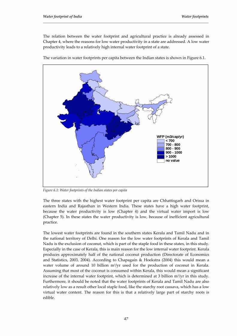
Water footprint of India Water footprints
The relation between the water footprint and agricultural practice is already assessed in Chapter 4, where the reasons for low water productivity in a state are addressed. A low water productivity leads to a relatively high internal water footprint of a state. The variation in water footprints per capita between the Indian states is shown in Figure 6.1.
WFP (m3/cap/yr)< 700700 - 800800 - 900900 - 1000> 1000no value
Figure 6.1: Water footprints of the Indian states per capita The three states with the highest water footprint per capita are Chhattisgarh and Orissa in eastern India and Rajasthan in Western India. These states have a high water footprint, because the water productivity is low (Chapter 4) and the virtual water import is low (Chapter 5). In these states the water productivity is low, because of inefficient agricultural practice. The lowest water footprints are found in the southern states Kerala and Tamil Nadu and in the national territory of Delhi. One reason for the low water footprints of Kerala and Tamil Nadu is the exclusion of coconut, which is part of the staple food in these states, in this study. Especially in the case of Kerala, this is main reason for the low internal water footprint. Kerala produces approximately half of the national coconut production (Directorate of Economics and Statistics, 2003, 2004). According to Chapagain & Hoekstra (2004) this would mean a water volume of around 10 billion m3/yr used for the production of coconut in Kerala. Assuming that most of the coconut is consumed within Kerala, this would mean a significant increase of the internal water footprint, which is determined at 3 billion m3/yr in this study. Furthermore, it should be noted that the water footprints of Kerala and Tamil Nadu are also relatively low as a result other local staple food, like the starchy root cassava, which has a low virtual water content. The reason for this is that a relatively large part of starchy roots is edible.
47

Water footprint of India Water footprints
The water footprint in Delhi is low because of the large percentage of the population living in urban area. Since a large part of the crops in Delhi are consumed as processed products, the intermediate consumption is high and the reported consumption low.
6.2 Water footprint by colour In Figure 6.2, the blue, green and gray components of the water footprints per capita are presented by state. The blue, green and gray water footprints of the states are tabulated in Appendix XIV.
0
200
400
600
800
1000
1200
1400
Andhra Pradesh
Assam Bih
ar
ChhattisgarhDelhi
Gujarat
Haryana
Himachal Pradesh
Jammu and K
ashmir
Jharkhand
Karnataka
Kerala
Madhya Pradesh
Maharashtra
Orissa
Punjab
Rajasthan
Tamil Nadu
Uttar Pradesh
Uttaranchal
West Bengal
Water footprint (m3/cap/yr)
gray
green
blue
Figure 6.2: Water footprints per capita and the contribution of the water colours for the Indian states during the period 1997‐2001. Figure 6.2 shows that the two states with the highest total water footprint, Chhattisgarh and Orissa, have the highest green water footprint, but one of the lowest blue water footprint. Furthermore, Figure 6.2 shows that Punjab and Haryana have the highest blue water footprint, but have a relatively low green water footprint. The total water footprint of India of 777 billion m3/yr consists for 227 billion m3/yr (29%) of blue water, for 459 billion m3/yr (59%) of green water and for 92 billion m3/yr (12%) of gray water. It is worth noticing that the calculated water footprint in this study is based on the consumption of approximately 82% of the crop production (see chapter 3.2). In the study of Chapagain & Hoekstra (2004), the total water footprint of the consumption of agricultural commodities of India is assessed at 927 billion m3/yr. 82% of this value is 760 billion m3/yr. Since the gray component is not taken into account in the study of Chapagain & Hoekstra, this value is compared to the sum of the blue and the green component of the water footprint in this study, which is 685 billion m3/yr. This shows that the water footprint of India in this study is 10% lower than the water footprint as calculated by Chapagain & Hoekstra (2004). A reason for this lower value in the current study can be the fact that the actual water use is calculated, while Chapagain & Hoekstra (2004) calculated the optimal water use.
48

Water footprint of India Water footprints
6.3 Water footprint by crop Besides the distinction between the blue, green and gray water footprint, the total water footprint can be divided into the water footprint of the individual crops. The contribution of the studied crops to the water footprints of the Indian states are presented in Figure 6.3.
0
200
400
600
800
1000
1200
1400
Andhra Pradesh
Assam Bih
ar
ChhattisgarhDelhi
Gujarat
Haryana
Himachal Pradesh
Jammu and K
ashmir
Jharkhand
Karnataka
Kerala
Madhya Pradesh
Maharashtra
Orissa
Punjab
Rajasthan
Tamil Nadu
Uttar Pradesh
Uttaranchal
West Bengal
Water footprint (m3/cap/yr)
cotton lint
edible oils
pulses
sugar
coarse cereals
wheat
rice
Figure 6.3: Water footprints per capita and the contribution of the different crops for the Indian states during the period 1997‐2001. Figure 6.3 shows that there is a relation between the water footprint and consumption pattern. The water footprint is significantly influenced by the fact that the staple food in a state consists of rice or wheat, or the fact that there is a high or low level of oil and sugar consumption. The magnitude of the water footprint of a state is determined by the average virtual water content of the crops that are consumed in that state.
6.4 Water footprint by region The internal, external and total water footprint of the four regions of India is given as a total and per capita in Table 6.3. In the calculation of the water footprint of a region, the interstate virtual water flows within a region are considered as part of the internal water footprint. Table 6.3: Water footprints of the consumption of agricultural commodities of the Indian regions
Total state region footprint Water footprint per capita States
Internal External Total Internal External Total unit 109 m3/yr m3/cap/yr year 1997‐2001 North 154 15 169 632 62 694 East 175 41 215 655 153 808 West 211 29 240 820 113 933 South 137 16 153 629 75 704 Total 658 119 777 658 119 777
49
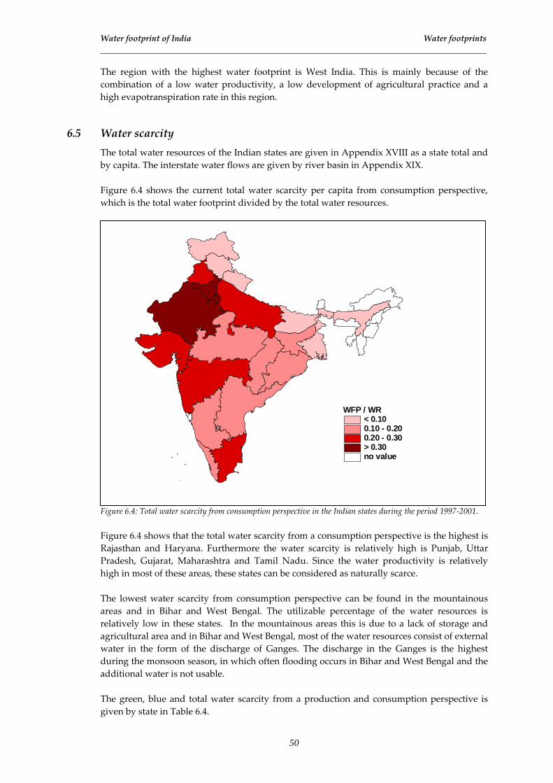
Water footprint of India Water footprints
The region with the highest water footprint is West India. This is mainly because of the combination of a low water productivity, a low development of agricultural practice and a high evapotranspiration rate in this region.
6.5 Water scarcity The total water resources of the Indian states are given in Appendix XVIII as a state total and by capita. The interstate water flows are given by river basin in Appendix XIX. Figure 6.4 shows the current total water scarcity per capita from consumption perspective, which is the total water footprint divided by the total water resources.
WFP / WR< 0.100.10 - 0.200.20 - 0.30> 0.30no value
Figure 6.4: Total water scarcity from consumption perspective in the Indian states during the period 1997‐2001. Figure 6.4 shows that the total water scarcity from a consumption perspective is the highest is Rajasthan and Haryana. Furthermore the water scarcity is relatively high is Punjab, Uttar Pradesh, Gujarat, Maharashtra and Tamil Nadu. Since the water productivity is relatively high in most of these areas, these states can be considered as naturally scarce. The lowest water scarcity from consumption perspective can be found in the mountainous areas and in Bihar and West Bengal. The utilizable percentage of the water resources is relatively low in these states. In the mountainous areas this is due to a lack of storage and agricultural area and in Bihar and West Bengal, most of the water resources consist of external water in the form of the discharge of Ganges. The discharge in the Ganges is the highest during the monsoon season, in which often flooding occurs in Bihar and West Bengal and the additional water is not usable. The green, blue and total water scarcity from a production and consumption perspective is given by state in Table 6.4.
50

Water footprint of India Water footprints
Table 6.4: blue and green water scarcity from consumption and production perspective
Water scarcity Consumption perspective Production perspective
States Blue Green Total Blue Green Total unit ― year 1997‐2001 Andhra Pradesh 0.10 0.18 0.13 0.10 0.21 0.14 Assam 0.01 0.22 0.03 0.00 0.21 0.02 Bihar 0.05 0.47 0.10 0.03 0.38 0.07 Chhattisgarh 0.05 0.24 0.13 0.04 0.26 0.14 Delhi 14.37 1.89 4.85 0.70 0.12 0.26 Gujarat 0.13 0.32 0.20 0.12 0.29 0.19 Haryana 0.52 0.28 0.40 0.90 0.54 0.71 Himachal Pradesh 0.02 0.07 0.04 0.01 0.05 0.02 Jammu & Kashmir 0.07 0.04 0.05 0.03 0.03 0.03 Jharkhand 0.10 0.26 0.17 0.03 0.17 0.10 Karnataka 0.10 0.21 0.15 0.10 0.20 0.15 Kerala 0.11 0.17 0.13 0.01 0.06 0.03 Madhya Pradesh 0.11 0.20 0.15 0.12 0.25 0.18 Maharashtra 0.17 0.32 0.25 0.15 0.33 0.24 Orissa 0.05 0.27 0.14 0.03 0.25 0.12 Punjab 0.24 0.32 0.26 0.45 0.65 0.51 Rajasthan 0.54 0.24 0.32 0.63 0.24 0.35 Tamil Nadu 0.29 0.17 0.22 0.29 0.19 0.23 Uttar Pradesh 0.18 0.34 0.23 0.20 0.43 0.27 Uttaranchal 0.05 0.07 0.06 0.04 0.10 0.07 West Bengal 0.03 0.41 0.07 0.03 0.43 0.07 Total India 0.14 0.22 0.18 0.13 0.23 0.18 Table 6.4 shows that the national blue, green and total water scarcity from consumption perspective closely matches the national blue, green and total water scarcity from production perspective. This is because the net international export of virtual water is relatively small in India. The high blue water scarcity from production perspective in Punjab, Haryana, Rajasthan and Tamil Nadu is line with the current status on water scarcity in the Indus, Luni and Cauvery river basins (Bobba et al., 1997; Rosegrant et al., 2002; Gupta & Deshpande, 2004; Falkenmark, 2005). In Table 6.4, it can be seen that the states with a high water scarcity from production perspective, Haryana, Punjab and Rajasthan, also have a relatively high water scarcity from consumption perspective.
6.6 Global water saving as a result of interstate trade The global water saving as a result of interstate trade in crops during the study period is given for the Indian states by colour and as a net total in Table 6.5.
51
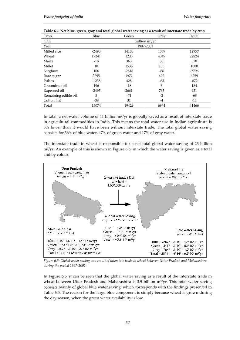
Water footprint of India Water footprints
Table 6.4: Net blue, green, gray and total global water saving as a result of interstate trade by crop Crop Blue Green Gray Total Unit million m3/yr Year 1997‐2001 Milled rice ‐2490 14108 1339 12957 Wheat 17241 1235 4349 22824 Maize ‐18 363 33 378 Millet 10 1536 135 1680 Sorghum 106 ‐2816 ‐86 ‐2796 Raw sugar 3795 1972 492 6259 Pulses ‐1238 428 ‐63 ‐872 Groundnut oil 196 ‐18 6 184 Rapeseed oil ‐2495 2661 765 931 Remaining edible oil 5 ‐71 ‐2 ‐68 Cotton lint ‐38 31 ‐4 ‐11 Total 15074 19429 6964 41466 In total, a net water volume of 41 billion m3/yr is globally saved as a result of interstate trade in agricultural commodities in India. This means the total water use in Indian agriculture is 5% lower than it would have been without interstate trade. The total global water saving consists for 36% of blue water, 47% of green water and 17% of gray water. The interstate trade in wheat is responsible for a net total global water saving of 23 billion m3/yr. An example of this is shown in Figure 6.5, in which the water saving is given as a total and by colour.
Figure 6.5: Global water saving as a result of interstate trade in wheat between Uttar Pradesh and Maharashtra during the period 1997‐2001. In Figure 6.5, it can be seen that the global water saving as a result of the interstate trade in wheat between Uttar Pradesh and Maharashtra is 3.9 billion m3/yr. This total water saving consists mainly of global blue water saving, which corresponds with the findings presented in Table 6.5. The reason for the large blue component is simply because wheat is grown during the dry season, when the green water availability is low.
52

Water footprint of India Water footprints
The interstate trade in milled rice is responsible for a net total global water saving of 13 billion m3/yr. An example of this is shown in Figure 6.6, in which the global water saving is given as a total and by colour.
Figure 6.6: Global water saving as a result of interstate trade in milled rice between Uttar Pradesh and Bihar during the period 1997‐2001. Figure 6.6 shows that the global water saving as a result of the interstate trade in milled rice from Uttar Pradesh to Bihar is 1.1 billion m3/yr. Figure 6.6 and Table 6.5 show that interstate trade in milled rice leads to global green and gray water saving, but to global blue water loss. The interstate trade in raw cane sugar is responsible for a net total global water saving of 6 billion m3/yr. In Figure 6.7 shows an example of water saving by colour and as a total, in which the interstate trade in raw cane sugar leads to global water loss.
Figure 6.7: Global water saving as a result of interstate trade in raw cane sugar between Uttar Pradesh and West Bengal during the period 1997‐2001.
53
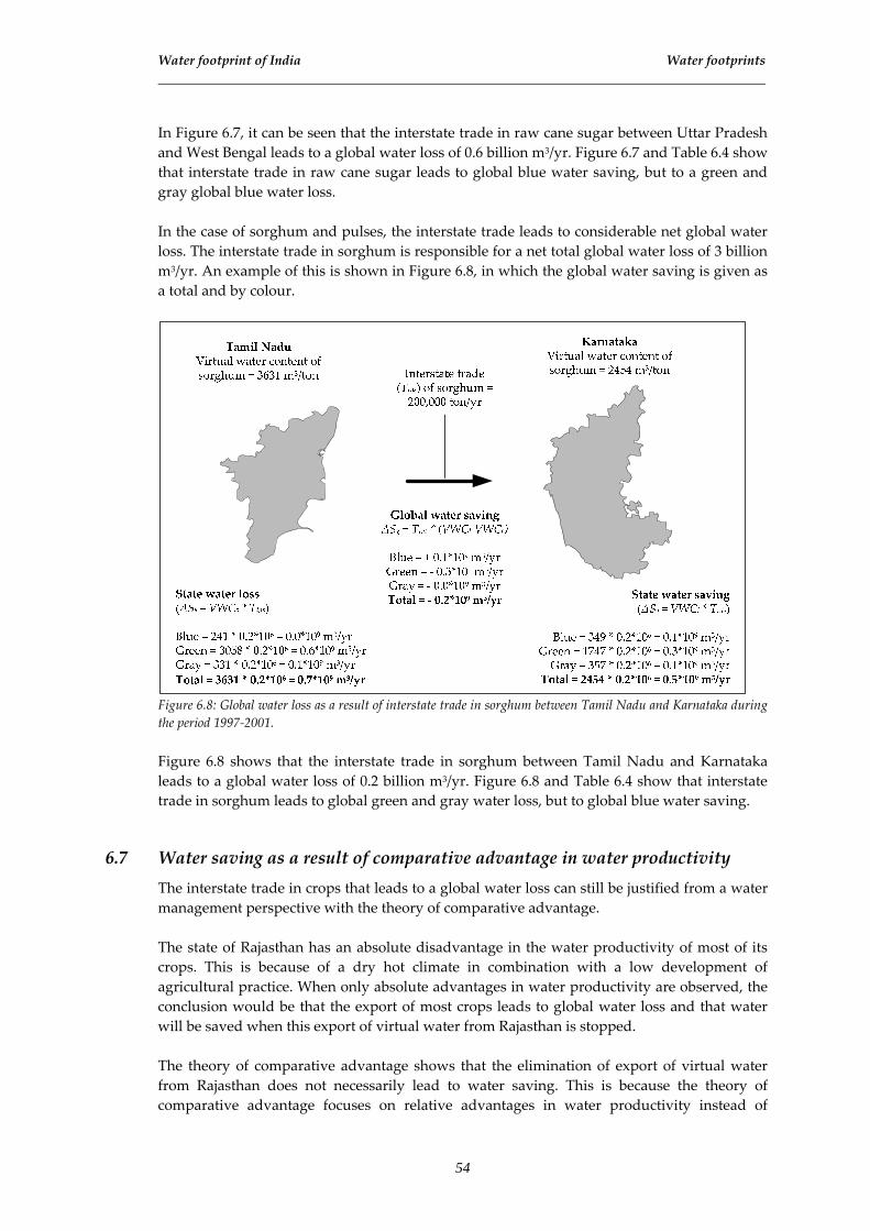
Water footprint of India Water footprints
In Figure 6.7, it can be seen that the interstate trade in raw cane sugar between Uttar Pradesh and West Bengal leads to a global water loss of 0.6 billion m3/yr. Figure 6.7 and Table 6.4 show that interstate trade in raw cane sugar leads to global blue water saving, but to a green and gray global blue water loss. In the case of sorghum and pulses, the interstate trade leads to considerable net global water loss. The interstate trade in sorghum is responsible for a net total global water loss of 3 billion m3/yr. An example of this is shown in Figure 6.8, in which the global water saving is given as a total and by colour.
Figure 6.8: Global water loss as a result of interstate trade in sorghum between Tamil Nadu and Karnataka during the period 1997‐2001. Figure 6.8 shows that the interstate trade in sorghum between Tamil Nadu and Karnataka leads to a global water loss of 0.2 billion m3/yr. Figure 6.8 and Table 6.4 show that interstate trade in sorghum leads to global green and gray water loss, but to global blue water saving.
6.7 Water saving as a result of comparative advantage in water productivity The interstate trade in crops that leads to a global water loss can still be justified from a water management perspective with the theory of comparative advantage. The state of Rajasthan has an absolute disadvantage in the water productivity of most of its crops. This is because of a dry hot climate in combination with a low development of agricultural practice. When only absolute advantages in water productivity are observed, the conclusion would be that the export of most crops leads to global water loss and that water will be saved when this export of virtual water from Rajasthan is stopped. The theory of comparative advantage shows that the elimination of export of virtual water from Rajasthan does not necessarily lead to water saving. This is because the theory of comparative advantage focuses on relative advantages in water productivity instead of
54

Water footprint of India Water footprints
absolute advantages in water productivity. The logic behind this theory is that when a state has an absolute disadvantage in water productivity of all crops, the maximum global benefit from the state water resources is created when these water resources are used to produce the crop, of which the water productivity has the least absolute disadvantage. In the period 1997‐2001, Rajasthan exported 0.10 million ton/yr of chickpeas to Punjab and 0.12 million ton/yr of rapeseed oil to Uttar Pradesh and imported 0.40 million ton/yr of wheat from Punjab and 0.50 million ton/yr of raw sugar from Uttar Pradesh. The global water saving as a result of interstate trade in chickpeas and wheat between Rajasthan and Punjab is shown in Figure 6.9.
Figure 6.9: Global water savings as a result of interstate trade in chickpeas and wheat between Rajasthan and Punjab the period 1997‐2001. Figure 6.9 shows that the interstate trade in wheat from Punjab to Rajasthan leads to global water saving and that the interstate trade in chickpeas from Rajasthan to Punjab leads to global water loss. The global water saving as a result of interstate trade in rapeseed oil and raw sugar between Rajasthan and Uttar Pradesh is shown in Figure 6.10.
55
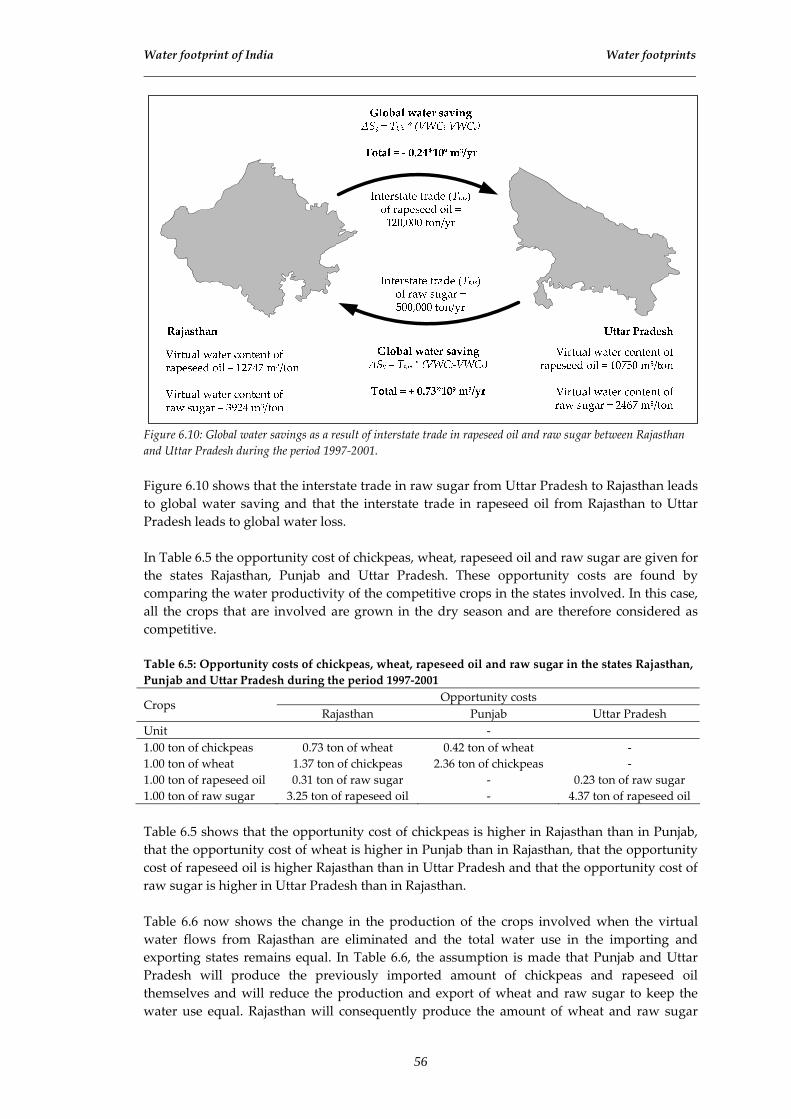
Water footprint of India Water footprints
Figure 6.10: Global water savings as a result of interstate trade in rapeseed oil and raw sugar between Rajasthan and Uttar Pradesh during the period 1997‐2001. Figure 6.10 shows that the interstate trade in raw sugar from Uttar Pradesh to Rajasthan leads to global water saving and that the interstate trade in rapeseed oil from Rajasthan to Uttar Pradesh leads to global water loss. In Table 6.5 the opportunity cost of chickpeas, wheat, rapeseed oil and raw sugar are given for the states Rajasthan, Punjab and Uttar Pradesh. These opportunity costs are found by comparing the water productivity of the competitive crops in the states involved. In this case, all the crops that are involved are grown in the dry season and are therefore considered as competitive. Table 6.5: Opportunity costs of chickpeas, wheat, rapeseed oil and raw sugar in the states Rajasthan, Punjab and Uttar Pradesh during the period 1997‐2001
Opportunity costs Crops
Rajasthan Punjab Uttar Pradesh Unit ‐ 1.00 ton of chickpeas 0.73 ton of wheat 0.42 ton of wheat ‐ 1.00 ton of wheat 1.37 ton of chickpeas 2.36 ton of chickpeas ‐ 1.00 ton of rapeseed oil 0.31 ton of raw sugar ‐ 0.23 ton of raw sugar 1.00 ton of raw sugar 3.25 ton of rapeseed oil ‐ 4.37 ton of rapeseed oil Table 6.5 shows that the opportunity cost of chickpeas is higher in Rajasthan than in Punjab, that the opportunity cost of wheat is higher in Punjab than in Rajasthan, that the opportunity cost of rapeseed oil is higher Rajasthan than in Uttar Pradesh and that the opportunity cost of raw sugar is higher in Uttar Pradesh than in Rajasthan. Table 6.6 now shows the change in the production of the crops involved when the virtual water flows from Rajasthan are eliminated and the total water use in the importing and exporting states remains equal. In Table 6.6, the assumption is made that Punjab and Uttar Pradesh will produce the previously imported amount of chickpeas and rapeseed oil themselves and will reduce the production and export of wheat and raw sugar to keep the water use equal. Rajasthan will consequently produce the amount of wheat and raw sugar
56

Water footprint of India Water footprints
that is no longer imported from Punjab and Uttar Pradesh and will reduce the production of chickpeas and rapeseed oil to keep the water use equal. Table 6.6: The change in crop production with the elimination of the export of chickpeas from Rajasthan to Punjab and the export of rapeseed oil from Rajasthan to Uttar Pradesh in the period 1997‐2001 when the total water use in the states remains equal
Rajasthan Punjab Uttar Pradesh Total Unit Million ton/yr Chickpeas ‐ 0.17 + 0.10 ‐ ‐ 0.07 Wheat + 0.24 ‐ 0.24 ‐ 0 Rapeseed oil ‐ 0.16 ‐ + 0.12 ‐ 0.04 Raw sugar + 0.52 ‐ ‐ 0.52 0 Table 6.6 shows that the elimination of export of chickpeas and rapeseed oil from Rajasthan to Punjab and Uttar Pradesh, leads to a decrease in crop production, while the water use remains equal. This means that although this export of chickpeas and rapeseed oil leads to global water loss, the water loss would be even larger when these export flows are eliminated. Another state that has an absolute disadvantage in the water productivity of most its crops is Madhya Pradesh. This is mainly because of the low development of agricultural practice. The theory of comparative advantage again shows that the export of some crops can still be justified from water management perspective in Madhya Pradesh. In the period 1997‐2001, Madhya Pradesh exported 0.12 million ton/yr of soybean oil and 0.40 million ton/yr of wheat to the rest of India and imported 1.30 million ton/yr of raw sugar and 0.40 million ton/yr of milled rice from the rest of India. The global water saving as a result of the interstate export of soybean oil and wheat from Madhya Pradesh and the interstate import of raw sugar and milled rice into Madhya Pradesh is shown in Figure 6.10.
Figure 6.11: Global water saving as a result of interstate trade in soybean oil, wheat, raw sugar and milled rice between Madhya Pradesh and the rest of India during the period 1997‐2001.
57

Water footprint of India Water footprints
Figure 6.11 shows that the interstate export of soybean oil and wheat from Madhya Pradesh leads to global water loss and that the interstate import of raw sugar and milled rice into Madhya Pradesh leads to global water saving. Table 6.7 shows the opportunity cost of soybean oil, milled rice, wheat and raw sugar for Madhya Pradesh and for the rest of India. These opportunity costs are found by comparing the water productivity of the competitive crops in the states involved. In this case, soybean oil and milled rice are seen as competitive because they are both grown in the wet season and wheat and raw sugar are seen as competitive because they are both grown in the dry season. Table 6.7: Opportunity costs of soybean oil, milled rice, wheat and raw sugar in Madhya Pradesh and whole India during the period 1997‐2001
Opportunity costs Crops
Madhya Pradesh India Unit ‐ 1.00 ton of soybean oil 0.88 ton of milled rice 1.64 ton of milled rice 1.00 ton of milled rice 1.13 ton of soybean oil 0.61 ton of soybean oil 1.00 ton of wheat 0.49 ton of raw sugar 0.63 ton of raw sugar 1.00 ton of raw sugar 2.04 ton of wheat 1.58 ton of wheat Table 6.7 shows that the opportunity cost of soybean oil and wheat is higher in Madhya Pradesh than in the rest of India and that the opportunity cost of milled rice and raw sugar is higher in the rest of India than in Madhya Pradesh. Table 6.8 now shows the change in production with the elimination of the virtual water flows from Madhya Pradesh when the total water use in the importing and exporting states remains equal. In Table 6.8, the assumption is made that the rest of India will produce the previously imported amount of soybean oil and wheat itself and will reduce the production and export of milled rice and raw sugar to keep the water use equal. Madhya Pradesh will consequently produce the amount of milled rice and raw sugar that is no longer imported and will reduce the production of soybean oil and wheat to keep the water use equal. Table 6.8: The change in crop production with the elimination of the interstate export of soybean oil and wheat from Madhya Pradesh in the period 1997‐2001 when the total water use in the states remains equal
Madhya Pradesh India Total Unit Million ton/yr Soybean oil ‐ 0.22 + 0.12 ‐ 0.10 Milled rice + 0.20 ‐ 0.20 0 Wheat ‐ 0.52 + 0.40 ‐ 0.12 Raw sugar + 0.25 ‐ 0.25 0 Table 6.8 shows that the elimination of the export of soybean oil and wheat from Madhya Pradesh to the rest of India, leads to a decrease in crop production, while the water use remains equal. This means that although this export of soybean oil and wheat leads to global water loss, the water loss would be even larger when these export flows are eliminated.
58

7. Food security: River interlinking versus increasing water productivity
7.1 Strategies for Indian water management The Indian population will be approximately 1.6 billion people in the year 2050 (United Nations, 2006). Furthermore, the average wealth in India is also growing rapidly. This will lead to an absolute increase in the food demand. From the perspective of water resources management, in which food production equals water use, there are in general three alternative strategies to meet the increasing food demand: • Water self sufficiency on state level • Water self sufficiency on national level • National virtual water import Here, water self sufficiency means that a state or nation only uses its current internal and external water resources for food self sufficiency. The first alternative is a situation where all Indian states are water self sufficient. This would mean that the consumption pattern should be shifted to those crops that yield the most with the water resources in the particular state. The second alternative is the situation where India is nationally water self sufficient and thus food self sufficient. This is more or less the current situation in which states are importing virtual water from other states. The third alternative is a situation in which water self sufficiency is no longer obtained and virtual water is imported from other countries. Falkenmark (1997, 2005) claims that, in the case of India, virtual water import will be necessary in the near future and that food self sufficiency as a goal will have to be given up. However, this alternative is currently not considered as an option by the Indian government. If India wants to remain food self sufficient with its rapidly growing population, given that there is a minimum of water use needed to produce the daily diet of the Indian people, water scarcity must be reduced. At the moment, the Indian government is considering the project of the Interlinking of Rivers (ILR). ILR aims to reduce the water scarcity in water deficit regions by increasing the local water resources with the import of water through the newly constructed connections of rivers.
59
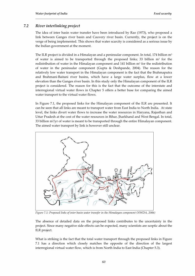
Water footprint of India Food security
7.2 River interlinking project The idea of inter basin water transfer have been introduced by Rao (1973), who proposed a link between Ganges river basin and Cauvery river basin. Currently, the project is on the verge of being implemented. This shows that water scarcity is considered as a serious issue by the Indian government at the moment. The ILR project is divided in a Himalayan and a peninsular component. In total, 174 billion m3 of water is aimed to be transported through the proposed links; 33 billion m3 for the redistribution of water in the Himalayan component and 141 billion m3 for the redistribution of water in the peninsular component (Gupta & Deshpande, 2004). The reason for the relatively low water transport in the Himalayan component is the fact that the Brahmaputra and Brahmani‐Baitani river basins, which have a large water surplus, flow at a lower elevation than the Ganges river basin. In this study only the Himalayan component of the ILR project is considered. The reason for this is the fact that the outcome of the interstate and interregional virtual water flows in Chapter 5 offers a better base for comparing the aimed water transport to the virtual water flows. In Figure 7.1, the proposed links for the Himalayan component of the ILR are presented. It can be seen that all links are meant to transport water from East India to North India. At state level, the links divert water flows to increase the water resources in Haryana, Rajasthan and Uttar Pradesh at the cost of the water resources in Bihar, Jharkhand and West Bengal. In total, 33 billion m3/yr of water is meant to be transported through the entire Himalayan component. The aimed water transport by link is however still unclear.
Figure 7.1: Proposed links of inter basin water transfer in the Himalayan component (NWDA, 2006) The absence of detailed data on the proposed links contributes to the uncertainty in the project. Since many negative side effects can be expected, many scientists are sceptic about the ILR project. What is striking is the fact that the total water transport through the proposed links in Figure 7.1 has a direction which closely matches the opposite of the direction of the largest interregional virtual water flow, which is from North India to East India (Chapter 5.3).
60

Water footprint of India Food security
Since the real and virtual flows are opposite to each other, the question rises if it is possible to eliminate both flows. This is done by taking away the dependency of food import of East India. Since water is not the limiting factor to the crop production in East India, an increase in water productivity in that region can lead to an increase in crop production. The question is whether this increase in water productivity in East India is possible.
7.3 Increasing water productivity
7.3.1 Potential yield An increase of the water productivity of a crop starts with the increase of the yield of a crop. This is possible when a significant gap exists between the current and potential yield of crop. Potential yield is defined here as the maximum yield that can be generated for a certain crop in a certain state when all needs for an optimal crop growth are supplied. The current yield of a crop depends on many factors; climate (the occurrence of drought or flooding and the amount of sun hours), irrigated or rain fed area, amount of fertilizer use, use of high yielding varieties, water salinity, access to energy (diesel pumps or electricity), tribal or non tribal area (Phansalkar & Verma, 2005) and soil type. We assume that the potential crop yield only depends on the climate. To demonstrate the result of a possible increase in yield, the example of milled rice in Bihar, Punjab and Uttar Pradesh is used here. This example is used because Bihar is largest importer of virtual water in East India, Punjab and Uttar Pradesh are the largest exporters of virtual water in North India, and milled rice is the crop with the largest contribution to the virtual water flow from North to East India. In this example only milled rice grown during kharif is taken into account, because this offers a better comparison between the states. During the study period, the yield of milled rice in Bihar during kharif is 1476 kg/ha. This results in an annual production of 5.1 million ton of milled rice. This is not enough to meet the annual consumption in Bihar of 7.1 million ton of milled rice. The deficit is mainly imported from the northern states Uttar Pradesh and Punjab. The yield of milled rice in Punjab in the study period is 3403 kg/ha and in Uttar Pradesh 2031 kg/ha. The difference in yield between the three states is mainly caused by the fraction irrigated area. In Punjab this fraction is 0.992, while in Uttar Pradesh this is 0.657 and in Bihar 0.393. In the irrigated areas, a rice variety is grown that requires relatively more fertilizer and a reliable supply of water (through irrigation), but has a considerable higher yield than the rice variety grown in the rain fed areas. This rice variety was introduced during the green revolution, which started in Asia in the late sixties of the previous century. Based on climatic factors, Uttar Pradesh and Bihar have a slightly lower potential yield than Punjab. Uttar Pradesh can potentially reach 95% of the maximum rice yield in Punjab and Bihar 92% (Aggarwal et al., 2000). Since we are only looking at the relative difference in crop yield, the assumption is made here that Punjab has already reached its potential yield, which is in this case 3403 kg/ha. This would mean that the potential yield in Uttar Pradesh is 3241 kg/ha and in Bihar 3144 kg/ha.
61

Water footprint of India Food security
7.3.2 Potential global water saving An increase in yield to the potential level leads to an increase in water productivity and thus in a decrease in virtual water content. The components of the crop water use of milled rice under the current growth conditions are calculated as presented in Table 7.1 (Appendix VI). Table 7.1: Calculation of the components of the crop water use of milled rice grown in the wet season under current growth conditions in Bihar, Punjab and Uttar Pradesh CWR CWUgreen IWR iaf CWUblue N use CWUgray Yield VWC unit m3/ha m3/ha m3/ha ‐ m3/ha kg/ha m3/ha kg/ha m3/ton year 1997‐2001 Bihar 7620 5878 1742 0.39 685 75 750 1476 4954 Punjab 8922 4234 4688 0.99 4651 103 1030 3403 2914 Uttar Pradesh 8207 5392 2816 0.66 1849 87 873 2031 3995 Assuming that it takes the same irrigated area fraction and nitrate use as in Punjab to achieve the potential yields in Bihar and Uttar Pradesh, the components of the crop water use of milled rice under optimal growth conditions are calculated as presented in Table 7.2. Table 7.2: Calculation of the components of the crop water use of milled rice grown in the wet season under optimal growth conditions in Bihar, Punjab and Uttar Pradesh CWR CWUgreen IWR iaf CWUblue N use CWUgray Yield VWC unit m3/ha m3/ha m3/ha ‐ m3/ha kg/ha m3/ha kg/ha m3/ton year 1997‐2001 Bihar 7620 5878 1742 0.99 1725 103 1030 3144 2747 Punjab 8922 4234 4688 0.99 4641 103 1030 3403 2914 Uttar Pradesh 8207 5392 2816 0.99 2788 103 1030 3241 2842 Table 7.1 and Table 7.2 show that the green crop water use (CWUgreen) remains the same, the blue crop water use (CWUblue) increases with the irrigated area fraction (iaf) and the gray crop water use (CWUgray) increases with the use of nitrate (N use). In Table 7.3, the blue, green, gray and total virtual water content of milled rice grown in the wet season in Punjab, Uttar Pradesh and Bihar is given for the current yields and for the potential yields. Table 7.3: Current and potential virtual water contents of milled rice grown in the wet season in Bihar, Punjab and Uttar Pradesh Bihar Punjab Uttar Pradesh VWC Current Potential Current Potential Current Potential unit m3/ton year 1997‐2001 Blue 464 549 1367 1367 910 860 Green 3982 1870 1244 1244 2654 1664 Gray 508 328 303 303 430 318 Total 4954 2747 2914 2914 3995 2842 In the current situation Bihar imports 1.2 million ton of milled rice from Uttar Pradesh and 0.8 million ton from Punjab. Actually Bihar also imports a little from Haryana, but this is neglected here.
62

Water footprint of India Food security
In Table 7.4, the reduction of the total water use as a result of the current interstate trade is presented for the current water productivities. Although the situation of food self sufficiency in Bihar is not possible given the current yield and land availability, this is still assumed in the calculation to show the reduction of the total water use as a result of interstate trade in the current situation. In this calculation, the total production and consumption is kept constant. Table 7.4: Reduction of total water use as a result of current interstate trade with the current water productivity of milled rice grown in the wet season in Bihar, Punjab and Uttar Pradesh while keeping the production and consumption constant
No interstate trade with current water productivities
Current interstate trade with current water productivities
Water use Water use States
P1 C2
blue green gray total P1 C2
blue green gray total
reduction total
water use
unit 106 ton/yr 109 m3/yr 106 ton/yr 109 m3/yr % year 1997‐2001 Bihar 7.1 7.1 3.3 28.3 3.6 35.2 5.1 7.1 2.4 20.3 2.6 25.3 +28.1 Punjab 7.7 2.3 10.5 9.6 2.3 22.4 8.5 2.3 11.6 10.6 2.6 24.8 ‐10.7 UP3 10.7 7.4 9.7 28.4 4.6 42.7 11.9 7.4 10.8 31.6 5.1 47.5 ‐11.2 Total 25.5 16.8 23.5 66.3 10.5 100.3 25.5 16.8 24.8 62.5 10.3 97.6 +2.7 1 P = production, 2 C = consumption, 3 UP = Uttar Pradesh Table 7.4 shows that with the current water productivities of milled rice in states involved, the current interstate trade pattern results in a reduction of the total water use of 2.7%. In Table 7.5, the reduction of the total water use as a result of the current interstate trade with the potential water productivities is presented. In this situation, food self sufficiency in Bihar is realistic given the potential yield and land availability. In this calculation the total production and consumption is again kept constant. Table 7.5: Reduction of total water use as a result of current interstate trade with the potential water productivity of milled rice grown in the wet season in Bihar, Punjab and Uttar Pradesh while keeping the production and consumption constant
No interstate trade with potential water productivities
Current interstate trade with potential water productivities
Water use Water use States
P1 C2
blue green gray total P1 C2
blue green gray total
reduction total
water use
unit 106 ton/yr 109 m3/yr 106 ton/yr 109 m3/yr % year 1997‐2001 Bihar 7.1 7.1 3.9 13.3 2.3 19.5 5.1 7.1 2.8 9.5 1.7 14.0 +28.2 Punjab 7.7 2.3 10.5 9.6 2.3 22.4 8.5 2.3 11.6 10.6 2.6 24.8 ‐10.7 UP3 10.7 7.4 9.2 17.8 3.4 30.4 11.9 7.4 10.2 19.8 3.8 33.8 ‐11.2 Total 25.5 16.8 23.6 40.7 8.0 72.3 25.5 16.8 24.6 39.9 8.1 72.6 ‐0.4 1 P = production, 2 C = consumption, 3 UP = Uttar Pradesh Table 7.5 shows that with the potential water productivities of milled rice in states involved, the current interstate trade results in no reduction of the total water use. Table 7.6 presents the reduction of the blue, green and gray water use as a result of the increase in water productivity, in the case of no interstate trade and the current interstate trade, and as a result of the current interstate trade, for the current and potential water productivities.
63

Water footprint of India Food security
Table 7.6: Reduction of the blue, green, gray and total water use as a result of current interstate trade with the current and potential water productivity of milled rice grown in the wet season in Bihar, Punjab and Uttar Pradesh while keeping the production and consumption constant Reduction of water use with the
increase in water productivity (%) Reduction of water use with current interstate trade of milled rice (%)
No interstate trade
Current interstate trade
Current water productivity
Potential water productivity
Blue water use ‐0.4 +0.8 ‐5.5 ‐4.2 Green water use +38.6 +36.2 +5.7 +2.0 Gray water use +23.8 +21.4 +1.9 +1.3 Total water use +27.9 +25.6 +2.7 ‐0.4
Table 7.6 shows that with the increase in water productivity of milled rice grown during the wet season in Bihar and Uttar Pradesh, a large volume of green and gray water is saved. Furthermore Table 7.6 shows that the current interstate trade in milled rice from Punjab and Uttar Pradesh to Bihar results in a green and gray water saving at the cost of a blue water loss. Table 7.4 and Table 7.5 show that by increasing the water productivities and eliminating the interstate trade of milled rice between the states involved, a water volume of 25.3 billion m3 is globally saved. Of this total, 21.8 billion m3 consists of green water saving. The remaining water saving consists of 1.2 billion m3/yr of blue water and 2.3 billion m3/yr of gray water. Green water saving may seem useless, as non used green water is lost though evaporation anyway and therefore has a low opportunity cost. In this example, the area used for milled rice growth in Bihar is reduced with the new yield and production volume. If the area, which is not used for milled rice growth anymore, remains unused, the green water saving is useless. If this area is used for more milled rice production, Rockström (2003) and Rockström & Gordon (2001, 2002) show that with an increase in yield and a fixed crop area, the total water productivity remains equal, but the productive part of the water productivity increases. In this example, this means that a relatively larger fraction of the green water, that is lost through evapotranspiration, contributes to the biomass of the crop. And by making better use of green water resources, the crop production can be reduced in places where relatively more blue water resources are needed for crop growth. In that case relative green water saving leads to absolute blue water saving. Apart from resulting in global water saving, the increase in water productivity in combination with the elimination of the current interstate trade also results in a change in water scarcity in the states of Bihar, Punjab and Uttar Pradesh. This change in water scarcity from production and consumption perspective in the states involved is presented in Table 7.7. Table 7.7: Change in blue, green and total water scarcity from consumption and production perspective in Bihar, Punjab and Uttar Pradesh with the increase in water productivity combined with the omission of the current interstate trade in milled rice between the states involved
Water scarcity from production perspective1 Water scarcity from consumption perspective1
Current situation2 Potential situation3 Current situation2 Potential situation3States B G T B G T B G T B G T
Bihar 0.03 0.38 0.07 0.03 0.27 0.06 0.05 0.47 0.10 0.04 0.29 0.07 Punjab 0.45 0.65 0.51 0.43 0.61 0.48 0.24 0.32 0.26 0.24 0.32 0.26 UP 0.20 0.43 0.27 0.19 0.34 0.23 0.18 0.34 0.23 0.17 0.29 0.21 1 B = blue water scarcity, G = green water scarcity, T = total water scarcity, 2 Source: Table 6.3, 3 Source: Appendix XX.
64

Water footprint of India Food security
Table 7.7 shows that increase in water productivity in combination with the omission of the current interstate trade in milled rice from Punjab and Uttar Pradesh to Bihar results in a reduction of the total water scarcity from production perspective in all three states. Furthermore, the water scarcity from consumption perspective is reduced in Bihar and Uttar Pradesh, because the internal water footprint in these two states in reduced through the increase in water productivity (see Appendix XX). The large decrease in the green water scarcity from both perspectives in Bihar seems strange, because the green crop water use can not be changed. The reason for this decrease is simply because the potential yield and the potential production of milled rice of 7.1 million ton/yr combined need a smaller crop area. In other words; with the potential yield and the current area cropped with milled rice, a production larger than 7.1 can be realised. Since our examples assume less agricultural area, less green water is used for evapotranspiration. Large increases in water productivity are also possible in the eastern states Chhattisgarh, Jharkhand, and Orissa, because the water productivity is generally low in these states.
7.4 River interlinking versus increasing water productivity
7.4.1 Potential reduction of water scarcity In Figure 7.2, water scarcity from production perspective in the present situation is compared to the current net import of virtual water for the northern and eastern states. Furthermore, the water scarcity is given for a situation without virtual water flows, in which the assumption is made that all consumed goods are produced within the state of consumption. For the importing states this means that the additional products in these states are produced at the same water efficiency level as the currently imported products and that the required agricultural area for this additional production of goods is available. In Figure 7.2, the national water scarcity is shown as a reference for relative water scarcity or water abundance.
-21000
0
21000
0.00 0.30 0.60
Figure 7.2: Water scarcity from production perspective versus net import virtual water import in the eastern and northern states of India.
65

Water footprint of India Food security
The gray lines in Figure 7.2 show the development of the water scarcity from production perspective if the exporting states stop exporting and the importing states start producing all previously imported goods themselves at the same efficiency as in the current exporting states. These lines show that the northern states remain relatively water scarce when they stop exporting virtual water and that the eastern states remain relatively water abundant when they become food self sufficient, which is line with our findings in Figure 6.4. Whether real water is transported from east to the north or less virtual water is transported from the north to the east, both options result in a reduction of water scarcity in the water scarce northern states at the expense of the water abundant eastern states. With the execution of the river interlinking project, the national average water scarcity is not directly changed. This is because the total national water use and total national water resources are not directly changed. The national water scarcity will only drop if the production in the areas with high water productivity increases at the cost of the production in the areas with low water productivity. This can only be realised in case the northern states can significantly increase their agricultural area. Since it is unclear how much water the northern states will actually receive through the ILR project, the reduction of the local water scarcity is hard to estimate. Based on the magnitude of the total water use compared to the magnitude of the total aimed real water transport, it seems impossible to bring the water scarcity from consumption perspective in the northern states below the national water scarcity with the ILR project. With the increase in water productivity in the water abundant states in combination with the elimination of the virtual water flows between the north and the east, the national average water scarcity can be reduced significantly. This is because the increase in water productivity reduces the total water footprint and therefore reduces the national water scarcity. In Figure 7.3, the four possible combinations of water scarcity from production perspective and net import of virtual water in a state are given. Here, a state is water abundant when the water scarcity in that state is below the national water scarcity and a state is water scarce when the water scarcity in that state is above the national water scarcity. Figure 7.3 also shows the consequences of the following strategies; the interlinking of rivers to transport water from water abundant areas to water scarce areas (A), the reduction of the food export in the water scarce states and of food import in the water abundant states (B), and the increase in water productivity (C).
66

Water footprint of India Food security
Water abundant stateswith net importof virtual water
Water abundant stateswith net exportof virtual water
Water scarce states with net importof virtual water
Water scarce stateswith net exportof virtual water
Net virtual water import
Net virtual water export
Water scarce
Water abundant
A,C
B
B
A,C
AC
BB+C
B+C B
A
C
Figure 7.3: The four combinations of water scarcity and net import of virtual water and the consequences of the following strategies; the interlinking of rivers to transport water from water abundant areas to water scarce areas (A), the reduction of the food export in the water scarce states and of food import in the water abundant states (B), and the increase in water productivity (C). Figure 7.3 shows that strategy A (ILR project) reduces the water scarcity in the water scarce states at the cost of the water abundant states. However, this is not enough to shift these states from water scarce to water abundant. Furthermore, Figure 7.3 shows that a combination of strategy B and strategy C reduces the water scarcity in the water scarce states and keeps the water scarcity in the water abundant states more or less constant, which means that the national water scarcity is reduced. As can be seen in Figure 7.3, the ILR project does not change the illogical situation from a water management perspective. Since the volume of water that can be transported is limited, the northern states can not become water abundant states. In order to change the illogical situation in which a large part of the water abundance in the eastern states is unutilized, the eastern states have to change from importing virtual water to exporting virtual water. If the agricultural area cannot be expanded, the only way to achieve this is to increase the water productivity. So all in all, the ILR project reduces local water scarcity, but will not significantly reduce the national water scarcity. Furthermore, in the case of milled rice, a trade flow is currently maintained that causes a global saving of green and gray water, but a global loss of blue water. From the perspective of logical water management, the transport of (blue) water only seems useful when a virtual water flow is maintained that results in global blue water saving. Yang (2003) indicates that there is a water resources threshold with respect to the import of cereals. Below this threshold, cereal import demand will increase exponentially with the decrease of the water availability per capita. This would mean that the northern states eventually are bound to reduce their export of virtual water and maybe even start importing virtual water.
67

Water footprint of India Food security
7.5 Water saving by changing crop patterns Finally, after presenting the option of reducing or increasing crop production and changing the direction of trade, the option of changing crop patterns in order to achieve global water saving is briefly discussed here. The theory of comparative advantage is used here to evaluate changes in crop patterns in the Indian states. The three important parameters in this evaluation are the potential yield, the water requirement and the water productivity of a crop. In Figure 7.4, the possible relation between the total water availability and the crop yield of two crops is shown. Here, the potential yield is found when the water availability equals the crop water requirement. The steepness of the curve represents the water productivity.
Figure 7.4: The possible relation between the total water availability for evapotranspiration and the crop yield for two crops in a state Figure 7.4 shows a situation in which crop 1 generates a higher yield in states with a relatively low water availability and crop 2 generates a higher yield in states with a relatively high water availability. When two crops are compared to each other, the boundary condition is that the crops are competitive. In the case of green water use, crops are only competitive if they are grown in the same season under comparable conditions. In the case of blue water use, crops can also be competitive if they are not grown in the same season, because blue water, especially in the form of groundwater, is available over a longer time period. In this study we have seen that in the current situation a large amount of milled rice as well as wheat is annually exported from Punjab and Uttar Pradesh to Bihar. Based on the theory of comparative advantage, Bihar must have a relative advantage in water productivity for one of these two crops. Because milled rice and wheat are not grown in during the same season, we only compare blue and gray water use. The opportunity costs of milled rice and wheat in the states Bihar, Punjab and Uttar Pradesh are presented in Table 7.8.
68
Water footprint of India Food security
Table 7.8: Opportunity costs of milled rice and wheat in the states Bihar, Punjab and Uttar Pradesh with the exclusion of green water productivity in the present situation during the period 1997‐2001
Opportunity costs Crops
Bihar Punjab Uttar Pradesh Unit ‐ 1.00 ton of milled rice 0.72 ton of wheat 3.00 ton of wheat 1.09 ton of wheat 1.00 ton of wheat 1.39 ton of milled rice 0.33 ton of milled rice 0.92 ton of milled rice From Table 7.8, the conclusion can be carefully made that Bihar currently has a relative advantage in blue and gray water productivity of milled rice when compared to Punjab and Uttar Pradesh. This means that the current trade flows of milled rice from Punjab and Uttar Pradesh to Bihar do not save water according to the theory of comparative advantage. It is worth noticing that the relative advantage in water productivity of a crop may change when the calculation is made for potential crop yields instead of actual crop yields. In this case this is not likely to happen, as Bihar receives significantly more green water than Punjab and Uttar Pradesh in the wet season, and therefore requires relatively less blue water for rice growth, and receives less green water than Punjab and Uttar Pradesh in the dry season, and therefore requires relatively more blue water for wheat growth. Of course it is still too early to make such a conclusion. We just want to indicate that a state like Bihar currently has no significant crop export, while there must be a crop in which Bihar has the highest relative advantage in water productivity. When looking at the current trade patterns and the theory of comparative advantage in the present situation, it might be useful to include the yield response factor of a crop in the analysis. The yield response factor is a constant that determines the sensitivity of the crop yield to water deficit (Doorenbos & Kassam, 1979). The comparison of relative advantages in water productivities of crops might not be sufficient to determine the optimal policies for maximizing the social benefits from limited water resources (Wichelns, 2001). This means that the availability of labour, capital and land in a state should also be taken into account in the calculation of relative advantages in water productivity of crops. This is because water is not always the limiting factor for the increase in crop production. In Bihar for example, there is enough water and labour, but the production is limited by the availability of land and capital.
69

70
8. Conclusion and discussion
8.1 Conclusion In the period 1997‐2001, the total virtual water flow as a result of interstate trade in agricultural commodities in India was 106 billion m3/yr, which was equal to 13% of the total water use in Indian agriculture. In the same period, the net international export from India was 15 billion m3/yr. A comparable study for China showed a total virtual water flow between Chinese sub‐regions of billion 128 m3/yr in the year 1999, which was equal to 10% of the total agricultural water use in China (Ma et al., 2006). In the period 1997‐2001, the global sum of international virtual water flows related to the trade of agricultural commodities was 987 billion m3/yr (Chapagain and Hoekstra, 2004). Of the total virtual water flow within India, 35% is due to the interstate trade of milled rice, 17% due the interstate trade of raw sugar and 14% due to the interstate trade of edible oils. The largest interregional net virtual water flow is 22 billion m3/yr and flows from the North India to the East India. As a result of international and interstate virtual water flows, the states Haryana, Madhya Pradesh, Punjab and Uttar Pradesh relatively have the largest negative virtual water balance and Bihar, Jharkhand and Kerala relatively have the largest positive virtual water balance. During our study period, the average water footprint of the consumption of agricultural commodities in India was 777 m3/cap/yr. In the same period, the average global water footprint of the consumption of agricultural commodities was 1066 m3/cap/yr, which did not include gray water use. The internal component is responsible for 658 m3/cap/yr and the external component for 119 m3/cap/yr. Furthermore, the blue component came to 227 m3/cap/yr, the green component to 459 m3/cap/yr and the gray component to 92 m3/cap/yr. A significant relation is visible between high water footprints and poor agricultural practice in the Indian states. The states Chhattisgarh and Orissa have the highest water footprint, which is mainly because of the low water productivity in the local rice production. For India as a whole, the water use from consumption perspective (777 billion m3/yr) was very close to the water use from production perspective (792 billion m3/yr). However, for individual states, like Bihar and Punjab, the consumption perspective often provides a very new picture if compared to the traditional production perspective. From the perspective of consumption, the water scarcity is the highest in the Rajasthan, Punjab, Uttar Pradesh, Tamil Nadu and Haryana. This means that the water resources of these states are closest to be exhausted in case of food self sufficiency. Because most of these states are also net exporters of virtual water, the water scarcity from a production perspective is even higher in these states. The total net global water saving as a result of the interstate trade in agricultural commodities in India was 41 billion m3/yr. This means the total water use in Indian agriculture was 5%
71

Water footprint of India Conclusion and discussion
lower than it would have been without interstate trade. The interstate trade in wheat alone already caused a global water saving of 23 billion m3/yr. It must be noted that the above mentioned numbers are somewhat uncertain, as this study is based on approximately 77% of the total crop production, 61% of the total production value and 84% of the total agricultural land use in India. Currently, India is considering implementing the concept of river interlinking. This concept means that water abundant regions will provide water to water scarce regions through the connection of rivers. Looking at the interlinking project from the perspective of the virtual water flows as calculated in this study, it can be seen that the proposed water transfer from East to North India has a direction exactly opposite to the direction of the virtual water flow as a result of interstate trade. In this study, it is demonstrated that an increase in water productivity in the water abundant states has a better chance of reducing the national water scarcity than the proposed water transfer. The river interlinking project mainly reduces local water scarcity, while water scarcity needs to be reduced significantly at a national level in order to remain food self sufficient as a nation. The only long term option for reducing the national water scarcity and remaining food self sufficient is to increase the water productivity in India. The largest opportunity for this increase lies in East India, where there is an abundance of water and a large increase in water productivity seems possible.
8.2 Discussion The methodology used in this study is largely based on earlier studies, which already calculated international virtual water flows and water footprints of nations (Hoekstra & Chapagain, 2007), virtual water flows and water footprints within a nation (Ma et al., 2006), the water footprint of a product (Chapagain et al., 2006) and global water saving as a result of international trade (Chapagain & Hoekstra, 2006). In this study, these previous methodologies are integrated and upgraded where possible. The main upgrades are the incorporation and assessment of green and blue water resources and the demonstration of how a consumption perspective on water management can quantitatively dispute water management strategies that are determined with a production perspective. The data that is used and generated in this study are rough and in some cases not complete. The roughness is due to the large scale of the study areas. Since one set of climatic parameters per state is used and only one set of crop parameters for whole India per season, the calculated virtual water content of crops do catch the main regional patterns but seem quite unreliable in the case of rain fed crops grown during the dry season. An incompleteness of this study is due the exclusion of crops. Important crops like coconuts, mango and pimento still represent a significant part of the total water use. Furthermore, the livestock products are excluded from this study. During the study period livestock products contributed a small part to the total water use in Indian agriculture. But the production and interstate of especially milk is increasing quickly. For example, Gujarat has an enormous milk production and where Gujarat in this study is assessed as an importer of virtual water, the inclusion of milk might well turn Gujarat into a net exporter of virtual water. The external water resources are very roughly estimated. The influence of large hill ranges like the Western Ghats are not taken into account. And in the assessment of the current water
72

Water footprint of India Conclusion and discussion
scarcity, the determination of the utilizable fraction of the total water resources will improve the reliability of the water scarcity at state level. This study covers the period 1997‐2001 and since patterns of crop production and crop trade change in time as a result of the average increase in welfare, the data that is used and generated might become less suitable to describe the present and future situations. By only looking at virtual water, the social benefits from limited water resources will not be maximized. So the fact that we are only looking at water resources is a limitation to this study. The availability of labour, capital and land should therefore be included in the relative advantage of the water productivity of crops. This might also change the importance of certain crops, which might not require much water, but may require much labour, land or capital. However, since the food self sufficiency is projected to become critical in the future, the present point of view is important for the future of India. It could be argued that the importance of water is small compared to the importance of land, labour, energy and capital. For example, irrigation in Bihar is currently executed with diesel pumps while in Punjab electricity is available, which is much cheaper. Water is a relatively costless resource, while products with virtual water embodied in it are seen as relatively costly. In other words; the import of real water feeds the perception of self sufficiency, whereas the import of virtual water feeds the perception of dependency. This study also misses a more detailed case study, which would have given a better insight in the practical implementation possibilities of both the river interlinking project and the increase in water productivity. Still we feel that this study gives a good indication of the virtual water flows in India, because it is indisputable that the direction of the largest virtual water flow is opposite to the direction of the aimed real water transport and that the water productivity in East India still has a large gap with the potential water productivity. In general, we can also dispute whether the exclusion of the alternative of national virtual water import to meet the increasing food demand is a smart move, because whatever internal solution will be chosen to meet the food demand in the future in India, the average water availability per capita in India will keep dropping with the increase in population.
73

74

References
Aggarwal, P.K., Talukdar, K.K., Mall, R.K., 2000. Potential yields of rice‐wheat system in the Indo‐Gangetic Plains if India. Consortium Paper Series 10. Rice‐wheat consortium for the Indo‐Gangetic Plains, New Delhi. Agrawal, G.D., 1999. Diffuse agricultural water pollution in India. Water Science and Technology, Vol. 39, p.33‐47. Allan, J.A., 1993. Fortunately there are substitutes for water otherwise our hydro‐political futures would be impossible. In: Priorities for water resources allocation and management, ODA, London, p. 13‐26. Allan, J.A., 1994. Overall perspectives on countries and regions. In: Rogers, P., Lydon, P. (editors). Water in the Arab World: perspectives and prognoses. Harvard University Press, Cambridge, Massachusetts, p. 65‐100. Allen, R.G., Pereira, L.S., Raes, D. and Smith, M., 1998. Crop evapotranspiration – Guidelines for computing crop water requirements. FAO Irrigation and Drainage Papers, Vol. 56, FAO, Rome, Italy. Bobba, A.G., Singh, V.P., Bengtsson, L., 1997. Sustainable Development of Water Resources in India. Environmental Management, Vol. 21, p. 367‐393. CDC, 2007. The Centers for Disease Control and Prevention, Atlanta, USA. www.cdc.gov/epiinfo/asia.htm Census of India, 2006. Census Data online. Registrar General and Census Commissioner, Government of India, New Delhi. http://www.censusindia.net CGWD, 1989. Ground water statistics. Central Groundwater Board, Ministry of Irrigation and Power, Department of Irrigation, Ministry of water resources, Government of India, Faridabad. Chandigarh Administration, 2006. Statistics. Chandigarh Administration, Chandigarh. http://sampark.chd.nic.in/images/statistics/SDP2005R6.pdf Chapagain, A.K., Hoekstra, A.Y., 2003. Virtual water flows between nations in relation to trade in livestock and livestock products. Value of Water Research Report Series No. 13, UNESCO‐IHE Institute for Water Education, Delft, the Netherlands. http://www.waterfootprint.org/Reports/Report13.pdf Chapagain, A.K, Hoekstra, A.Y., 2004. Water footprints of nations. Value of Water Research Report Series No. 16, UNESCO‐IHE Institute for Water Education, Delft, the Netherlands. http://www.waterfootprint.org/Reports/Report16Vol1.pdf Chapagain, A.K., Hoekstra, A.Y., 2006. Water saving through international trade of agricultural products. Hydrol. Earth Syst. Sci., 10, p.455‐468. Chapagain, A.K., Hoekstra, A.Y., Savenije, H.H.G., Gautam, R., 2006. The water footprint of cotton consumption: An assessment of the impact of worldwide consumption of cotton products on the water resources in the cotton producing countries. Ecological Economics 60, p. 186‐203. Chaturvedi, M.C., 1985. Water resources of India – an overview. Sadhana. Vol. 8, p. 13‐38.
75
Water footprint of India References
CIA, 2006. The World Factbook. Central Intelligence Agency, Government of United States of America, Washington D.C. https://www.cia.gov/cia/publications/factbook/geos/in.html Dastane, N.G., 1978. Effective rainfall in irrigated agriculture. FAO Irrigation and Drainage Papers. Vol. 25, FAO, Rome, Italy. Directorate of Economics and Statistics, 2003. Agricultural Statistics at a Glance. Agricultural Statistics Division, Directorate of Economics and Statistics, Ministry of Agriculture, Government of India, New Delhi. Directorate of Economics and Statistics, 2004. Agricultural Statistics at a Glance. Agricultural Statistics Division, Directorate of Economics and Statistics, Ministry of Agriculture, Government of India, New Delhi. Directorate of Rice Development, 2006a. Status Paper on Rice. Ministry of Agriculture, Government of India, Patna. http://www.dacnet.nic.in/rice Directorate of Rice Development, 2006b. Statistical Handbook. Ministry of Agriculture, Government of India, Patna. http://www.dacnet.nic.in/rice Directorate of Rice Development, 2006c. Productivity Analysis. Ministry of Agriculture, Government of India, Patna. http://www.dacnet.nic.in/rice Directorate of Pulses Development, 2006a. Varieties of pulses. Ministry of Agriculture, Government of India, Bhopal. http://dacnet.nic.in/pulses/APY‐website.pdf Directorate of Pulses Development, 2006b. Statistics. Ministry of Agriculture, Government of India, Bhopal. http://dacnet.nic.in/pulses/ VARIETIES‐Web%20site.pdf Directorate of Wheat Development, 2006. Statistics. Ministry of Agriculture, Government of India, Ghaziabad. http://dacnet.nic.in/dwd/wheat_prod1/wheat‐annx3.pdf Dohlman, E., Persaud, S., Landes, R., 2003. India’s Edible Oil Sector: Imports Fill Rising Demand. United States Department of Agriculture, Washington D.C. Doorenbos, J., Kassam, A.H., 1979. Yield Response to Water. FAO Irrigation and Drainage Papers. Vol. 33, FAO, Rome, Italy. http://www.fao.org/AG/AGL/aglw/cropwater/part.stm EPA, 2006. List of drinking water contaminants: groundwater and drinking water. US Environmental Protection Agency, Washington D.C. Falkenmark, M., Rockström, J., 1993. Curbing rural exodus from tropical drylands. Ambio 22, p.427‐437. Falkenmark, M., 1997. Meeting water requirements of an expanding world population. Phil. Trans. R. Soc. Lond. B. 352, p. 929‐936. Falkenmark, M., Lannerstad, M., 2005. Consumptive water use to feed humanity – curing the blind spot. Hydrology and Earth System Sciences, Vol.9, p. 15‐28. FAO, 2003. Review of the World Water Resources by Country. Water Reports 23. Food and Agricultural Organization of the United Nations, Rome, Italy. FAO, 2005. Fertilizer use by crop in India. Food and Agricultural Organization of the United Nations, Rome, Italy. FAO, 2006a. ‘FAOSTAT on‐line database’, Food and Agriculture Organization of the United Nations, Rome, Italy
76

Water footprint of India References
FAO, 2006b. CROPWAT model. Food and Agriculture Organization of the United Nations, Rome, Italy. http://www.fao.org/ag/AGL/aglw/cropwat.stm FAO, 2006c. CLIMWAT database. Food and Agriculture Organization of the United Nations, Rome, Italy. http://www.fao.org/ag/AGL/aglw/climwat.stm FAO, 2006d. Technical Conversion Factors for Agricultural Commodities. Food and Agriculture Organization of the United Nations, Rome, Italy. http://www.fao.org/WAICENT/FAOINFO/ECONOMIC/ESS/pdf/tcf.pdf FAO, 2006e. AQUASTAT database, Food and Agriculture Organization of the United Nations, Rome, Italy FAORAP, 2006. Regional Data Exchange System on food and Agricultural Statistics in Asia and the Pacific Countries. Regional Office for Asia and the Pacific, Food and Agricultural Organization, Bangkok, Thailand. Gupta, S.K., Deshpande, R.D., 2004. Water for India in 2050: first‐order assessment of available options. Current Science, Vol.86, No.9. Hoekstra, A.Y., Chapagain, A.K., 2007. Water footprints of nations: Water use by people as function of their consumption pattern. Water Resources Management 21, p.35‐48. Hoekstra, A.Y., Hung, P.Q., 2004. Globalisation of water resources: international virtual water flows in relation to crop trade. Global Environmental Change 15, p.45‐56. IISR, 2006. Statistics. Indian Institute of Sugar Cane Research, Lucknow. http://iisr.nic.in IITM, 2006. Data. Indian Institute of Tropical Meteorology, Pune. http://www.tropmet.res.in IMD, 2006. Normal rainfall maps. India Meteorological Department, New Delhi. http://www.imd.ernet.in/section/climate/annual‐rainfall.htm Ma, J., Hoekstra, A.Y., Wang, H., Chapagain, A.K., Wang, D., 2006. Virtual versus real water transfers within China. Phil.Trans.R.Soc.B., Vol.361, p.835‐842. Ministry of Water Resources, 2006a. Ground Water pollution. Ministry of Water Resources, Government of India, New Delhi. Ministry of Water Resources, 2006b. Water statistics. Ministry of Water Resources, Government of India, New Delhi. Ministry of Water Resources, 2006c. River basin maps. Ministry of Water Resources, Government of India, New Delhi. NSSO, 1997. Consumption of Some Important Commodities in India 1993‐1994. National Sample Survey Organisation Report 404, Department of Statistics, Ministry of Statistics & Programme Implementation, Government of India, New Delhi. NSSO, 1998. Household Consumer Expenditure and Employment Situation in India in 1997. National Sample Survey Organisation Report 442, Department of Statistics, Ministry of Statistics & Programme Implementation, Government of India, New Delhi. NSSO, 1999. Household Consumer Expenditure and Employment Situation in India in 1998. National Sample Survey Organisation Report 448, Department of Statistics, Ministry of Statistics & Programme Implementation, Government of India, New Delhi.
77

Water footprint of India References
NSSO, 2001a. Level and Pattern of Consumer Expenditure in India 1999‐2000. National Sample Survey Organisation Report 457, Department of Statistics, Ministry of Statistics & Programme Implementation, Government of India, New Delhi. NSSO, 2001b. Consumption of Some Important Commodities in India 1999‐2000. National Sample Survey Organisation Report 461, Department of Statistics, Ministry of Statistics & Programme Implementation, Government of India, New Delhi. NSSO, 2002. Household Consumer Expenditure and Employment – Unemployment Situation in India 2000‐2001. National Sample Survey Organisation Report 476, Department of Statistics, Ministry of Statistics & Programme Implementation, Government of India, New Delhi. NSSO, 2003. Household Consumer Expenditure and Employment – Unemployment Situation in India 2001‐2002. National Sample Survey Organisation Report 481, Department of Statistics, Ministry of Statistics & Programme Implementation, Government of India, New Delhi. NSSO, 2005. Sarvekshana, Journal of National Sample Survey Organisation, 88th Issue Vol XXV No.4 & Vol XXVI Vol.1. Department of Statistics, Ministry of Statistics & Programme Implementation, Government of India, New Delhi. NWDA, 2006. Inter Basin Water Transfer Proposals. National Water Development Agency. A Society under Ministry of Water Resources, Government of India, New Delhi. Phansalkar, S.J., Verma, S., 2005. Mainstreaming the Margins – Water‐centric Livelihood Strategies for Revitalizing Tribal Agriculture in Central India. Angus & Grapher, New Delhi. Planning Commission, 2002. Tenth Five Year Plan 2002‐2007. Planning Commission, Government of India, New Delhi. http://planningcommission.nic.in/ Postel, S.L., Daily, G.C., Ehrlich, P.R., 1996. Human Appropriation of Renewable Fresh Water. Science, Vol. 271, p.785‐788. Price, G.K., Landes, R., Govindan, A., 2003. India’s Pulse Sector: Results of Field Research. United States Department of Agriculture, Washington D.C. Radhakrishna, B.P., 2003. Linking of major rivers of India – Bane or boon? Current Science, Vol. 84, p. 1390‐1394. Rao, K.L., 1973. India’s Water Wealth. Orient Longman, New Delhi. Ricardo, D., 1817. On the Principles of Political Economy and Taxation. John Murray, Albemarle‐street, London. Rockström, J., Gordon, L., 2001. Assessment of Green Water Flows to Sustain Major Biomes of the World: Implications for Future Ecohydrological Landscape Management. Phys. Chem. Earth (B), Vol.26, No.11‐12, p. 843‐851. Rockström, J., Gordon, L., 2002. The Role of Green Water in Sustaining Ecological Functions – A Global Assessment. Water and Ecology, GAIA 11, No.4, p.267‐272. Rockström, J., 2003. Water for food and nature in drought‐prone tropics: vapour shift in rain‐fed agriculture. Phil. Trans. R. Soc. Lond. B. 358, p. 1997–2009. Rosegrant, M.V., Cai, X., Cline, S.A., 2002. World Water and Food to 2025. International Food Policy Research Institute, Washington D.C., USA.
78

Water footprint of India References
United Nations, 2004. World population prospects: The 2004 Revision, Volume III: Analytical Report. United Nations Department of Economic and Social Affairs, New York, USA. Wackerhagel, M., Rees, W., 1996. Our ecological footprint: Reducing human impact on the Earth. New Society Publishers, Gabriola Island, BC, Canada. Wichelns, D., 2001. The role of ‘virtual water’ in efforts to achieve food security and other national goals, with an example from Egypt. Agricultural Water Management 49, p.131‐151. Wichelns, D., 2007. Virtual Water: An Economic Perspective. In: Trimble, S.W. (ed.) Encyclopedia of Water Science, Taylor & Francis, New York. Article in press. World Bank, 2006. India at a Glance 2005. Data & Statistics, World Bank, Washington D.C., USA. http://siteresources.worldbank.org/INTSARMACECOGRO/34004333‐1148990480174/21048623/India.pdf Yang, H., Reichert, P., Abbaspour, K.C., Zehnder, A.J.B., 2003. A Water Resources Threshold and Its Implications for Food Security. Environmental Science & Technology. Vol. 37, p. 3048‐3054.
79