Task Specialization in U.S. Cities from 1880-2000∗

Guy MichaelsLondon School of Economics and CEP†

Ferdinand RauchUniversity of Oxford and CEP‡

Stephen J. ReddingPrinceton University and CEP§

August 25, 2017

Abstract

We develop a new methodology for quantifying the tasks undertaken within occupations using over3,000 verbs from more than 12,000 occupational descriptions in the Dictionary of Occupational Titles(DOTs). Using micro-data from the United States from 1880-2000, we nd an increase in the employmentshare of interactive occupations within sectors over time that is larger in metro areas than non-metroareas. We interpret these ndings using a model in which reductions in transport and communicationcosts induce urban areas to specialize according to their comparative advantage in interactive tasks. Wepresenting suggestive evidence relating increases in employment in interactive occupations to improve-ments in transport and communication technologies. Our ndings highlight a change in the nature ofagglomeration over time towards an increased emphasis on human interaction.

KEYWORDS: Economic Development, Human Interaction, Urbanization.JEL CLASSIFICATION: N92, O18, R12

∗We are grateful to the Centre for Economic Performance and Princeton University for research support. We are also grateful toGilles Duranton and Matt Turner for sharing data. We thank William D. Caughlin and George Kupczak for their help with data. Wealso thank the editor, four referees, Don Davis, Gilles Duranton, Gene Grossman, Gordon Hanson, Marco Manacorda, Alan Manning,Nathan Nunn, Vernon Henderson, Rick Hornbeck, Gianmarco Ottaviano, Steve Pischke, Esteban Rossi-Hansberg, Yona Rubinstein,Will Strange, Nancy Qian, Tony Venables and seminar and conference participants at Copenhagen, the London School of Economics,MIT, NARSC, Oxford, Sorbonne and Sussex for helpful comments and suggestions. The usual disclaimer applies.

†CEP, LSE, Houghton Street, WC2A 2AE, London, UK. Email: g.michaels@lse.ac.uk. Tel: +44(0)20-7852-3518.‡Department of Economics, University of Oxford, Manor Road, Oxford, OX1 3UQ. Email: ferdinand.rauch@economics.ox.ac.uk.

Tel: +44(0)77214-88037.§Fisher Hall, Princeton, NJ 08540. Email: reddings@princeton.edu. Tel: +1(609) 258-4016.

1

1 Introduction

Agglomeration forces are widely understood to play a central role in sustaining the dense concentrations of

population observed in urban areas. Much less is known about the detailed tasks undertaken in urban areas

and how these have changed over time. Yet understanding the task content of employment in urban and

rural areas is central to evaluating alternative theories of agglomeration and assessing the likely impact of

improvements in transport and communication technologies on spatial concentrations of economic activity.

In this paper, we provide new evidence on the detailed tasks undertaken by workers in urban and rural areas

over a long historical time period in the United States (U.S.). We develop a new methodology for measuring

the individual tasks undertaken within occupations using the verbs from occupational descriptions in the

Dictionary of Occupational Titles (DOTs). We implement this methodology using micro data on employment

in disaggregated occupations and sectors in metro and non-metro areas from 1880-2000.

To measure the individual tasks undertaken within each occupation, we use over 3,000 verbs from more

than 12,000 occupational descriptions in both historical and contemporary editions of the Dictionary of Oc-

cupational Titles (DOTs). Using these verbs, we nd a systematic change in the composition of employment

across tasks in urban versus rural areas over time. We quantify this change in task content using the meaning

of verbs from Roget’s Thesaurus, as the standard reference for English usage. In both metro and non-metro

areas, we nd a systematic reallocation of employment over time towards interactive occupations, which in-

volve tasks described by verbs that appear in thesaurus categories concerned with thought, communication

and inter-social activity. At the beginning of our sample period, metro areas actually have lower shares of

employment in interactive occupations than non-metro areas. Over time, employment growth in interactive

occupations is much higher in metro areas, so that by the end of our sample period the initial pattern of

specialization is reversed, and metro areas are more interactive than non-metro areas. This increasing inter-

activeness of employment at higher population densities is observed not only between metro and non-metro

areas but also across metro areas of dierent population densities. While in 1880 there is little relationship

between specialization in interactive occupations and population density, by 2000 this relationship is positive,

strong and statistically signicant. Taken together, these results suggest that human interaction has become

increasingly important in agglomerations of economic activity over time.

To interpret these empirical results, we develop a model of the spatial distribution of employment across

occupations, sectors and locations. The model features trade in the nal good produced by each sector and

in the tasks undertaken by the occupations within each sector. When the costs of trading tasks between

locations are prohibitively high, all tasks are performed where the nal good is produced. As the costs of

trading tasks fall, it becomes feasible to unbundle production across locations and trade tasks between them. If

agglomeration forces are stronger for interactive tasks, densely-populated urban locations have a comparative

advantage in interactive tasks, which implies that reductions in task trade costs induce them to specialize

2

in more-interactive occupations, while more sparsely-populated rural locations specialize in less-interactive

occupations.

We provide empirical evidence on the relationship between changes in the interactiveness of employment

and the major innovations in transport and communication technology that occurred during our sample

period. Following the award of Alexander Graham Bell’s patent for the telephone in 1886, the U.S. telephone

network grew rapidly in the opening decades of the twentieth century.1 After the award of Karl Benz’s patent

for the internal combustion engine in 1879 and after the passage of the Federal Aid Road Act of 1916 and the

Federal Highway Act of 1921, the U.S. road network and automobile use expanded rapidly over the same

period.2 We examine the implications of these new transport and communication technologies by combining

county data on employment by occupation and sector for 1880 and 1930 with newly-collected county data on

telephone use and the road network in the 1930s. We develop instruments for the geographical dissemination

of both technologies. For the telephone, we use its network properties to construct an instrument based

on proximity to nodes on the American Telegraph and Telephone’s (AT&T) company’s long distance trunk

network, whose construction was inuenced by the strategic objectives of connecting the nation as a whole.

For roads, we use the 1922 “Pershing Map” of highway routes of military importance for coastal and border

defense.3 We provide suggestive evidence connecting increases in the interactiveness of employment to the

diusion of these new technologies predicted by our instruments.

Our paper is related to a number of literatures. We build on the wider literature on agglomeration

economies, as surveyed in Duranton and Puga (2004) and Rosenthal and Strange (2004). One strand of this

literature emphasizes dierences in the composition of economic activity between urban and rural areas.

Studies emphasizing the role of human capital and skills in promoting agglomeration include Glaeser and

Saiz (2004), Glaeser and Resseger (2010), Bacolod, Blum and Strange (2009a), Glaeser, Ponzetto and Toblo

(2014) and Moretti (2004). Particular types of skills are highlighted in Bacalod, Blum and Strange (2009b),

which introduces the concept of soft skills that enable agents to interact in cities and industry clusters. More

generally, the role of idea generation and exchange is emphasized in Davis and Dingel (2012), which develops

a system of cities model in which costly idea exchange is the agglomeration force.

Another line of research has distinguished dierent dimensions along which cities specialize. Duranton

and Puga (2005) provides theory and evidence that in recent decades cities have shifted from specializing by

sector – with integrated headquarters and plants – to specializing mainly by function - with headquarters

and business services clustered in larger cities and plants clustered in smaller areas.4 Rossi-Hansberg, Sarte

and Owens (2009) develops a model in which rms choose locations of their headquarters and production fa-1See, for example, John (2010). The electric telegraph was patented much earlier in 1837 by Samuel Morse and the U.S. telegraph

network was largely complete by 1880 (see Standage 2007).2See, for example, Swift (2011).3Following the Federal Aid Highway Act of 1921, the Bureau of Public Roads commissioned General John J. Pershing to draw up

a map of roads of military importance in the event of war, as discussed further below.4See Henderson (1974) for the classic analysis of industry specialization and the size distribution of cities.

3

cilities, and argues that the increased separation of these locations accounts for observed changes in patterns

of residential and business activity. Ota and Fujita (1993) models the distinction between the front-unit (e.g.

business oce) and back-unit (e.g. plant or back-oce) of rms and explores its implications for city struc-

ture. Helsley and Strange (2007) explicitly analyzes the vertical integration decision of the rm in conjunction

with its location decision. Fujita and Tabuchi (1997) provides evidence that the increased separation of head-

quarters and production has contributed to observed changes in the distribution of economic activity across

Japanese regions.5 Related research has examined the impact of roads and urban growth (e.g. Baum-Snow

2007 and Duranton and Turner 2012) and the implications of innovations in communication technologies for

cities (e.g. Pool 1977, Fischer 1992, Gaspar and Glaeser 1998, Leamer and Storper 2001).

Our analysis is also related to the task-based approach to the labor market, including in particular Autor,

Levy and Murnane (2003, henceforth ALM), Acemoglu and Autor (2011), Autor and Handel (2009), Autor

(2013), Gray (2013), and Deming (2017). This research has developed measures of the task content of em-

ployment based on numerical scores from the Dictionary of Occupations (DOTs), such as “Direction, Control

and Planning (DCP).” Prior to this research, the canonical model of the labor market in terms of skilled and

unskilled labor had assumed that technological change is skill-biased. In contrast, this task-based approach

recognizes that the direction of technological change is endogenous, as emphasized in Acemoglu (1998) and

Acemoglu (2002). Therefore the extent to which new technologies complement or substitute for skills or

tasks can change over time. In the labor literature, Autor, Katz, and Krueger (1998) argue that there was an

acceleration in the skill-bias of technical change in the 1980s and 1990s. In the historical literature, several

studies have argued that technical change often replaced rather than complemented skilled artisans in the

nineteenth-century, including Hounshell (1985), James and Skinner (1985) and Mokyr (1992).6

Relative to each these lines of research, our main contribution is to develop a new approach for measuring

individual production tasks that uses the verbs from occupational descriptions and their meanings. Using

this new methodology, we are able to track the production tasks performed by workers at a much higher

resolution than has hitherto been possible. We use our approach to provide evidence on changes in the task

content of employment over a much longer historical time period than previously considered. We also apply

this approach to the organization of economic activity in urban and rural areas separately.

The remainder of the paper is structured as follows. Section 2 discusses the data. Section 3 introduces our

methodology and presents our main empirical results on changes in the task content of employment in urban5Other dimensions of specialization in urban areas examined in existing research include localization versus urbanization exter-

nalities (e.g. Jacobs 1969, Henderson 2003); the division of labor (e.g. Duranton and Jayet 2011); diversied versus specialized cities(e.g. Duranton and Puga 2001); employment in newly-created occupations (e.g. Lin 2011); and agglomeration versus rm selection(in particular Combes et al. 2012).

6In their classic study of the race between technology and skills, Goldin and Katz (2008) present evidence that manufacturingtechnologies were skill complementary in the early-twentieth century, but may have been skill substituting prior to that time. Insubsequent work, Katz and Margo (2014) report some evidence of de-skilling in manufacturing during the nineteenth-century, butnd a reallocation of employment towards high-skill jobs for the aggregate economy as a whole.

4

and rural areas over time. Section 4 outlines a theoretical framework for interpreting these empirical results

that points to the role played by transportation and communication technologies. Section 5 provides further

evidence on explanations for the observed changes in the task content of employment and their relationship

with changes in transportation and communication technologies. Section 6 concludes.

2 Data

Our empirical analysis uses two main sources of data. The rst is individual-level records from the U.S.

Population Census for twenty-year intervals from 1880-2000 from Integrated Public Use Microdata Series

(IPUMS): see Ruggles et al. (2010). These census micro data report individuals’ location, occupation and

sector, as well as other demographic information. We use these data to determine whether an individual is

located in a metro area as well as the occupation and sector in which an individual is employed. A metro area

is dened as a region consisting of a large urban core together with surrounding communities that have a

high degree of economic and social integration with the urban core.7 We weight individuals by their person

weights to ensure the representativeness of the sample. Our main dataset is a panel from 1880-2000 that uses

information on the share of employment within an occupation and sector in metro areas. To provide evidence

on improvements in communication and transportation technologies, we also use long-dierenced data from

1880-1930, aggregating our individual-level data to the county level.

We use the standardized 1950 occupation classication from IPUMS, which distinguishes eleven two-digit

occupations (e.g. “Clerical and Kindred”) and 281 three-digit occupations (e.g. “Opticians and Lens Grinders

and Polishers”). We also use the standardized 1950 sector classication from IPUMS, which distinguishes

twelve two-digit sectors (e.g. “Finance, Insurance and Real Estate”) and 158 three-digit sectors (e.g. “Motor

Vehicles and Motor Vehicle Equipment”).8 Since we are concerned with employment structure, we omit

workers who do not report an occupation and a sector (e.g. because they are unemployed or out of the labor

force). We also exclude workers in agricultural occupations or sectors, because we compare task specialization

in urban and rural areas over time, and agriculture is unsurprisingly overwhelmingly located in rural areas.9

We use time-varying denitions of metro areas to ensure that they correspond to meaningful economic units.

However, we also report robustness tests, in which we hold the sample composition of metro areas constant

over time, and in which we use administrative cities whose boundaries are more stable over time.

Our second main data source is the Dictionary of Occupational Titles (U.S. Department of Labor 1991),

which contains detailed descriptions of more than 12,000 occupations. Following Autor et al. (2003), previous7From 1950 onwards, the denitions of metropolitan areas are those constructed by the Census Bureau. Before 1950, IPUMS

applies to the historical population data the same criteria as used by the Census Bureau from 1950 onwards.8See IPUMS for the full concordance between two-digit and three-digit occupations and sectors. While both occupation and sector

classications are standardized by IPUMS, there are a small number of occupations and sectors that enter and exit the sample overtime. All our results are robust to restricting attention to occupations and sectors that are present in all years.

9Our key ndings, however, are robust to the inclusion of these agricultural workers. For further analysis of the relationshipbetween urbanization and structural transformation away from agriculture, see Michaels et al. (2012).

5

research using DOTs typically uses the numerical scores that were constructed for each occupation by the

Department of Labor (e.g. a Non-routine Interactive measure based on the Direction, Control and Planning

of Activities (DCP) numerical score). In contrast, we use verbs from the detailed occupational descriptions

in DOTs to directly measure the tasks performed by workers in each occupation. We use a list of over 3,000

English verbs from “Writing English,” a company that oers English language consulting.10 This approach

enables us to provide a rich analysis of the tasks undertaken in urban and rural areas using the verbs and

occupational descriptions without being restricted to the numerical scores. Nonetheless, we also compare our

measures of occupational characteristics to those from the numerical scores. We match the DOTs occupations

to the three-digit occupations in our census data using the crosswalk developed by ALM. In our baseline

specication, we use a time-invariant measure of tasks based on the occupational descriptions from the digital

edition of the 1991 DOTs, which ensures that our results are not driven by changes in language use over time.

In sensitivity checks, we also report results using digitized occupational descriptions from the rst edition of

the DOTs in 1939 (U.S. Department of Labor 1939).

We complement these two main data sources with information from a variety of other sources. We use

the standard reference for word usage in English (Roget’s Thesaurus) to quantify the meanings of verbs

from the occupational descriptions.11 We use ArcGIS shapeles from the National Historical Geographical

Information System (NHGIS) to track the evolution of county boundaries over time. We also use measures of

improvements in transport and communication technologies. We measure the length of roads in each county

using a georeferenced 1931 road map (Gallup 1931).12 At the beginning of our sample in 1880, most U.S.

roads were little more than dirt tracks (see, for example, Swift 2011) and widespread paved road construction

only occurred following the Federal Aid Road Act of 1916 and the Federal Highway Act of 1921. Therefore

we use the 1931 map to construct a measure of the growth of the paved road network from 1880-1930. We

measure the number of residence telephones in each county in 1935 using newly-digitized data from American

Telephone and Telegraph Company (AT&T 1935). The telephone was not patented until 1876 just before the

beginning of our sample period and the telephone network developed rapidly from 1890 onwards (see, for

example, Fischer 1992). Therefore we use the data on telephones to construct a measure of the growth of

telephones from 1880-1930. To address the concern that the road network could be inuenced by changes

in the interactiveness of economic activity, we use an instrument based on the “Pershing” map of highway

routes of military importance for coastal and border defense. To address similar concerns for the telephone,

we use an instrument based on proximity to primary and secondary outlets on AT&T’s long distance trunk

network, whose construction was inuenced by the strategic objective of connecting the nation as a whole.10See http://www.writingenglish.com/englishverbs.htm.11We use a computer-searchable edition of Roget (1911) from the University of Chicago.12Recent economics research on the U.S. road network has largely concentrated on the later development of the interstate highway

system, as in Baum-Snow (2007), Michaels (2008) and Duranton and Turner (2012).

6

3 Empirical Evidence on Task Specialization

In this section, we present our main results on changes in the task content of employment in urban and rural

areas over time. In subsection 3.1, we begin by characterizing changes in specialization across occupations

and sectors in metro areas relative to non-metro areas over our long historical time period. In subsection

3.2, we introduce our new methodology for measuring individual production tasks using the verbs from

occupational descriptions. In subsection 3.3, we explain how we quantify the meanings of these verbs using

Roget’s thesaurus, and introduce a new measure of the interactiveness of the tasks undertaken by workers.

In subsection 3.4, we demonstrate the robustness of our results across a range of specications.

3.1 Specialization Across Occupations and Sectors

To provide some initial motivating evidence of changes in specialization across occupations and sectors in

metro areas relative to non-metro areas, we estimate the following regression for each year t separately using

data across occupations o and sectors s:

MetroShareost = µot + ηst + εost, (1)

where MetroShareost is the share of employment in metro areas in occupation o, sector s and year t; observa-

tions are weighted by person weights; µot are occupation-year xed eects; ηst are sector-year xed eects;

and εost is a stochastic error. We normalize the sector-year and occupation-year xed eects so that they

each sum to zero in each year, and hence they capture deviations from the overall mean in each year. While

we estimate the above regression using a share as the left-hand side variable so that the estimated coecients

have a natural interpretation as frequencies, we nd a very similar pattern of results in a robustness test in

which we use a logistic transformation of the left-hand side variable: MetroShareost/(1−MetroShareost).

The occupation-year xed eects (µot) capture the average probability of being in a metro area for work-

ers in each occupation in each year, after controlling for dierences across sectors in metro probabilities.

Similarly, the sector-year xed eects (ηit) capture the average probability of being located in a metro area

for workers in each sector in each year, after controlling for dierences across occupations in metro proba-

bilities. The sector and occupation xed eects are separately identied because there is substantial overlap

in occupations and sectors, such that each sector contains multiple occupations and each occupation is em-

ployed in several sectors.13 We estimate this regression using both the aggregate (two-digit) and disaggregate

(three-digit) denitions of occupations and sectors discussed above.

As reported in Table 1 for two-digit occupations and sectors, we nd substantial changes in specialization

across occupations and sectors in metro areas relative to non-metro areas over time. From Panel A, in 1880,

“Clerical and Kindred” workers were the most likely to be located in metro areas. In contrast, by 2000, “Clerical13The average three-digit sector employs workers from 111 three-digit occupations, while the average three-digit occupation

contains workers employed in 81 sectors.

7

and Kindred” workers were ranked only fourth, and “Professional and Technical” workers were the most

likely to be located in metro areas. From 1880-2000, declines in ranks were observed for “Craftsmen” (from 2

to 6) and “Operatives” (from 3 to 7), while increases in ranks were observed for “Professional and Technical”

workers (from 7 to 1) and “Managers, Ocials and Proprietors” (from 6 to 3). As apparent from the rst and

fourth columns of the table, these changes in ranks reect substantial changes in the probabilities of workers

in individual occupations being located in metro areas over time.

Since the regression (1) includes sector-year xed eects, these changes in the metro probabilities for each

occupation are not driven by changes in sector composition, but rather reect changes in the organization

of economic activity within sectors. Nonetheless, we also observe substantial changes in sector structure

in metro areas relative to non-metro areas over time. From Panel B, declines in ranks from 1880-2000 were

observed for “Wholesale and Retail Trade” (from 2 to 6) and “Manufacturing” (from 4 to 10). In contrast,

increases in ranks from 1880-2000 were observed for “Transportation, Communication and Other Utilities”

(from 6 to 3) and “Business and Repair Services” (from 9 to 1).

In Figures A1 and A2 of the web appendix, we show the evolution of the occupation and sector coecients

across each of the twenty-year intervals in our data. While “Professional and Technical” workers display an

increased propensity to locate in metro areas from 1880-1960, the probability that “Managers, Ocials and

Proprietors” are located in urban areas increases particularly sharply from 1940-2000. In contrast, the likeli-

hood that “Craftsmen” are found in metro areas declines throughout our sample period, while the probability

for “Clerical and Kindred” workers declines from 1900 onwards, and the probability for “Service” workers

initially rises until 1920 and later declines until around 1960.

Such changes in specialization are not limited to the aggregate categories considered so far, but are also

found using more disaggregated measures of occupations and sectors. In Table A1 of the web appendix,

we report the results of estimating the regression (1) including three-digit-occupation-year and three-digit-

sector-year xed eects. Panels A and B report the twenty occupations within the largest increases and

decreases respectively in the within-sector probability of being located in a metro area from 1880-2000. Both

the top agglomerating occupations in Panel A and the top dispersing occupations in Panel B are diverse

and span multiple sectors. For example, leading agglomerating occupations include “Editors and Reporters,”

“Buyers and Department Heads,” and “Judges and Lawyers,” while prominent dispersing occupations are

“Book Binders,” “Welders and Flame Cutters,” and “Upholsterers.” In our empirical analysis below, we provide

evidence on the systematic characteristics shared by occupations that agglomerate versus disperse over time.

3.2 Measuring the Tasks Undertaken by Occupations

We now introduce our new methodology for individual production tasks using the detailed descriptions from

more than 12,000 disaggregated occupations included in the DOTs. We use the verbs from each occupation’s

8

description to measure the tasks performed by workers within that occupation, because verbs capture an

action (bring, read, walk, run, learn), an occurrence (happen, become), or a state of being (be, exist, stand),

and hence capture the task being performed. To focus on persistent characteristics of occupations and abstract

from changes in word use over time, our baseline analysis uses time-invariant occupational descriptions from

the 1991 digital edition of the DOTs. While the tasks undertaken within each occupation can change over time,

the relative task content of occupations is likely to be more stable. To provide evidence on the extent to which

this is the case, we have also digitized the occupational descriptions from the rst edition of the DOTs in 1939.

Although the descriptions of occupations are less detailed and the boundaries between occupations are less

clear in the historical DOTs, we nd a similar pattern of results using both sets of occupational descriptions,

as discussed further below.

The rst step of our procedure uses a list of over 3,000 English verbs from “Writing English,” a company

that oers English language consulting. Using this list of verbs, we search each occupational description in

the 1991 DOTs for occurrences of each verb in the rst-person singular (e.g. (I) talk), third-person singular

(e.g. (she) talks) or present participle (e.g. (he is) talking).14 For example, the occupational description for an

Economist is:

“ECONOMIST: Plans, designs, and conducts research to aid in interpretation of economic re-

lationships and in solution of problems arising from production and distribution of goods and

services: Studies economic and statistical data in area of specialization, such as nance, labor, or

agriculture. Devises methods and procedures for collecting and processing data, utilizing knowl-

edge of available sources of data and various econometric and sampling techniques. Compiles

data relating to research area, such as employment, productivity, and wages and hours. Reviews

and analyzes economic data in order to prepare reports detailing results of investigation, and to

stay abreast of economic changes ...,”

where the words detected by our procedure as capturing the tasks performed by an economist are italicized.15

Note that sometimes the rst-person singular, third-person singular or present participle forms of a verb

have the same spelling as the corresponding adjectives and nouns (e.g. “prepare reports”). In this case, our

procedure treats these adjectives and nouns as verbs. To the extent that the use of the same word as an

adjective or noun is closely related to its use as a verb, both uses are likely to capture the tasks performed.

From this rst step, we obtain the number of occurrences of each verb for each DOTs occupation. We

next match the more than 12,000 DOTs occupations to IPUMS standardized 1950 occupations using the cross-

walk developed by ALM. Finally, we calculate the frequency with which each verb v is used for each IPUMS14An emerging literature in economics and the social sciences uses textual search as the basis for quantitative analysis: see for

example Gentzkow et al. (2012) on political inuence and Michel et al. (2011) on culture.15As an indication of the wide coverage of our list of over 3,000 verbs, only 1,830 appear in the 1991 DOTs occupational descriptions.

9

occupation o:

VerbFreqvo =Appearances of verb v matched to o

Appearances of all verbs matched to o,

where we focus on the frequency rather than the number of verb uses to capture the relative importance of

tasks for an occupation and to control for potential variation in the length of the occupational descriptions

matched to each IPUMS occupation.

We provide evidence on changes in task specialization in metro areas relative to non-metro areas over time

by estimating the following regression for each verb v and year t separately using data across occupations o

and sectors s:

MetroShareost = αvtVerbFreqvo + ηvst + εost, (2)

where MetroShareost is again the share of employment in metro areas in occupation o, sector s and year t;

VerbFreqvo is dened above for verb v and occupation o; ηvst are verb-sector-year xed eects; and εost is a

stochastic error.

The coecient of interest αvt captures a conditional correlation: the correlation between occupations’

shares of employment in metro areas and their frequency of use of verb v. The verb-sector-year xed eects

(ηvst) control for dierences across sectors in the frequency of verb use and for dierences across sectors and

over time in the concentration of employment in metro areas. Since VerbFreqvo is time invariant, a rise in

αvt over time implies that employment in occupations using that verb is increasingly concentrating in metro

areas within sectors over time.

In Panels A and B of Table 2, we report for each year the ten verbs with the highest and lowest standardized

coecient αvt (the estimated coecient multiplied by the standard deviation of VerbFreqvo).16 As apparent

from Panel A, we nd substantial changes in the tasks most concentrated in metro areas within sectors over

time. In 1880, the verbs with the highest metro employment shares typically involve physical tasks such as

“Braid,” “Sew,” “Stretch” and “Thread.” By 1920, the top ten verbs include an increased number of clerical tasks,

such as “Bill,” “File,” “Notice,” and “Record.” By 1980 and 2000, the leading metro verbs include a proliferation

of interactive tasks, such as “Analyze,” “Advise,” “Confer” and “Report.” As shown in Panel B, we also nd

some changes in the tasks least concentrated in metro areas, although here the pattern is less clear cut (e.g.

“Tread” appears from 1880-1960 and “Turn” appears from 1960-2000).

3.3 Quantifying Task Specialization

The approach developed in the previous section allows us to provide a detailed characterization of the tasks

performed in urban and rural areas using the full list of verbs and all occupational descriptions. In this

section, we now develop a quantitative measure of task specialization based on the meanings of these verbs.16We nd a similar pattern of results just using the estimated coecients instead of the estimated coecients times the standard

deviation of VerbFreqvo.

10

To do so, we use the online computer-searchable version of Roget’s Thesaurus (1911), which has been the

standard reference for English language use for more than a century, and explicitly classies words according

to their underlying concepts and meanings. Roget’s classication was inspired by natural history, with its

hierarchy of Phyla, Classes, Orders and Families. Therefore words are grouped according to progressively

more disaggregated classications that capture ever more subtle variations in meaning. A key advantage of

this classication is that it explicitly takes into account that words can have dierent meanings depending

on context by including extensive cross-references to link related groups of words.17

Roget’s Thesaurus is organized into “Classes” which are further disaggregated into the progressively ner

partitions of “Divisions,” “Sections” and “Categories.” There are 6 classes, 10 divisions, 38 sections and around

1,000 categories.18 The rst three classes cover the external world: Class I (Abstract Relations) deals with

ideas such as number, order and time; Class II (Space) is concerned with movement, shapes and sizes; and

Class III (Matter) covers the physical world and humankind’s perception of it by means of the ve senses.

The last three classes relate to the internal world of human beings: the human mind (Class IV, Intellect), the

human will (Class V, Volition) and the human heart and soul (Class VI, Emotion, Religion and Morality).

To characterize the meaning of each verb v, we use the frequency with which it appears in each partition

k of Roget’s Thesaurus:

ThesFreqvk =Appearances of verb v in category k of thesaurus

Total appearances of verb v in thesaurus, (3)

where the partition k could be a class, division, section or category of the thesaurus; our use of a frequency

takes into account that each verb can have multiple meanings and provides a measure of the relative impor-

tance of each meaning. In counting verb appearances, we make use of the thesaurus’s structure, in which

words with similar meanings appear under each thesaurus Category in a list separated by commas or semi-

colons. Based on this structure, we count appearances of a verb that are followed by a comma or semi-colon,

which enables us to abstract from appearances of a word in idioms that do not reect its common usage.19

Combining the frequency with which a verb appears in each occupation’s description (VerbFreqvo in

the previous section) and the frequency with which the verb appears in each category of the thesaurus

(ThesFreqvk), we construct a quantitative measure of the extent to which the tasks performed in an occu-17For further discussion of the genesis of Roget’s Thesaurus, see for example Hüllen (2003).18Division is an intermediate level in between class and section, which is only used in the thesaurus to disaggregate Classes IV and

V. In particular, “Class IV Words Relating to the Intellectual Faculties” is split into “Division I Formation of Ideas” and “Division IICommunication of Ideas.” Additionally, “Class V Words Relating to the Voluntary Powers” is split into “Division I Individual Volition”and “Division II Intersocial Volition.” Classes I-III and VI are not disaggregated into divisions.

19For example, the verb “Consult” appears in six thesaurus Categories. The entry followed by a comma is 695 Advice, whichcaptures the word’s meaning. Entries not followed by a comma correspond to idiomatic uses not closely related to the word’smeaning: 133 Lateness (“consult one’s pillow”); 463 Experiment (“consult the barometer”); 707 Aid (“consult the wishes of”); 943Selshness (“consult one’s own pleasure”); 968 Lawyer (“juris consult [Latin]”). We do not require that a verb is preceded by acomma or semi-colon, because this would exclude the rst verb listed under each thesaurus category.

11

pation involve the concepts from each thesaurus category :

TaskContentko =∑v∈V

VerbFreqvo × ThesFreqvk.

We use this measure to examine changes in task specialization in metro areas relative to non-metro areas

over time by estimating an analogous regression for each thesaurus category k and year t as for each verb

and year in the previous section:

MetroShareost = βktTaskContentko + ηkst + εost, (4)

where MetroShareost is the share of employment in metro areas in occupation o, sector s and year t; TaskContentko

is dened above for thesaurus partition k and occupation o; ηkst are thesaurus-category-year xed eects;

and εost is a stochastic error.

The coecient of interest βkt again captures a conditional correlation: the correlation between occupa-

tions’ shares of employment in metro areas and their frequency of use of verbs in thesaurus category k. The

thesaurus-category-sector-year xed eects (ηkst) control for dierences across sectors in the frequency of

use of thesaurus categories and dierences across sectors and over time in the concentration of employment

in metro areas. Since TaskContentko is time invariant, a rise in βkt over time implies that employment in

occupations using that category of the thesaurus is increasingly concentrating in metro areas within sectors

over time.

In Table 3, we report the estimation results for the thirty-eight sections of the thesaurus (denoted by S),

organized by the 6 classes (denoted by C) and 10 divisions of the thesaurus (denoted by D). We calculate the

standardized coecient for each thesaurus section (the estimated coecient βkt multiplied by the variable’s

standard deviation) and report the ranking of these standardized coecients in 1880 and 2000 as well the

dierence in rankings between these two years (1880 minus 2000).20 Since the thesaurus section with the

highest standardized coecient is assigned a rank of one, positive dierences in rankings correspond to

thesaurus sections that are becoming more concentrated in metro areas within sectors over time.

The results in Table 3 reveal a sharp change the relative ranking of thesaurus sections involving the

external world (Classes I-III) and those involving the internal world of human beings (Classes IV-VI). In 1880,

the top-ve thesaurus sections most concentrated in metro areas included: Quantity (Class I), Time (Class

I), Dimensions (Class II), Matter in General (Class III), and Aections in General (Class VI). In contrast, in

2000, the top-ve thesaurus sections were: Nature of Ideas Communicated (Class IV), Special Intersocial

Volition (Class V), Extension of Thought (Class IV), Reasoning Processes (Class IV), and Results of Reasoning

(Class IV). The correlation between the rankings of the thesaurus sections in 1880 and 2000 is negative and

statistically signicant (-0.63).20Again we nd a similar pattern of results using just the estimated coecient instead of the estimated coecient times the

standard deviation of TaskContentko.

12

Positive changes in ranks in Table 3 are typically concentrated in thesaurus Classes IV and V, which

correspond to the human mind and the human will respectively. These Classes include Class IV, Division

1 (Formation of Ideas), Class IV, Division 2 (Communication of Ideas) and Class V, Division 2 (Intersocial

Volition). We summarize this combination of tasks – thought, communication and intersocial activity – as

“interactiveness.” Our interpretation is that interaction inherently involves each of these components: think-

ing for oneself, communication these thoughts, and communicating them to other people in a social envi-

ronment. We exclude Class V, Division 1 (Individual Volition) from our denition of interactiveness, because

it is more concerned with individual reection and decision making (e.g. motive, habit, willingness, choice)

rather than interaction between people. Although some of the categories in Class VI could be interpreted as

interactive (e.g. Section III, “Sympathetic Aections”), the other categories within this class seem to point

more to contemplation and introspection than interaction between people (e.g. “Aections in General,” “Per-

sonal Aections,” “Moral Aection,” and “Religious Aection”). Furthermore, the interpersonal relationships

described in “Sympathetic Aections” seem to largely concern relationships outside of work.

Therefore, we measure the interactiveness of an occupation using the frequency with which verbs appear

in that occupation’s description and the frequency with which those verbs appear in Divisions 1 and 2 of

Class IV and Division 2 of Class V of the thesaurus:

Interactiveo =∑v∈V

FreqVerbvo × FreqInteractivev, (5)

where FreqVerbvo is the frequency with which verb v is used for occupation o from above; FreqInteractivev

is the frequency with which verb v appears in these partitions of the thesaurus (computed as in (3)). We also

report results below for all four divisions of Classes IV and V of the thesaurus.

In Panels A and B of Table 4, we report the top ten and bottom ten interactive occupations using our

measure. While any single quantitative measure of interactiveness is unlikely to capture the full meaning

of this concept, the occupations identied by our procedure as having high and low levels of interactiveness

appear intuitive. “Buyers and Department Heads”, “Clergymen” and “Pharmacists” arguably perform more

interactive tasks than “Blasters and Powdermen”, “Roofers and Slaters” and “Welders and Flame Cutters.”

In Figure 1, we measure the interactiveness of metro areas, non-metro areas and the economy as a whole

using the employment-weighted average of interactiveness for each occupation. In this measure, interactive-

ness only diers between metro and non-metro areas to the extent that they have dierent distributions of

employment across occupations:

Interactivejt =

O∑o=1

EojtEjt

Interactiveo, j ∈ M,N , (6)

where j indexes a type of location and we again denote metro areas by M and non-metro areas by N ; Eojt

corresponds to employment in occupation o in location type j ∈ M,N in year t.

13

In 1880, metro and non-metro areas have similar levels of interactiveness, with if anything metro areas

having lower interactiveness than non-metro areas. Over time, interactiveness increases in both sets of lo-

cations, but this increase is greater in metro areas than in non-metro areas. This increase in the relative

interactiveness of metro areas is particularly sharp from 1900-1920, which coincides with the dissemination

of improvements in communication and transport technologies in the form of the telephone and roads and

the automobile. In our empirical analysis below, we provide further evidence on the extent to which changes

in interactiveness are related to these new communication and transport technologies.

3.4 Robustness

Having presented our baseline evidence of an increase in the interactiveness of employment in metro areas

relative to non-metro areas over time, we now document the robustness of this nding across a range of

dierent specications.

3.4.1 1939 DOTs

Our baseline specication measures the task content of employment using time-invariant occupational de-

scriptions from the 1991 DOTs. While this approach ensures that our ndings are not driven by changes

in language use over time, it assumes that the relative task content of occupations is persistent over time.

One concern is that the interactiveness of occupations could have changed over time and these changes in

interactiveness could be correlated with occupations’ shares of employment in metro areas.

To address this concern, we replicated our analysis using the rst edition of the DOTs from 1939. We

digitized the occupational descriptions in the 1939 DOTs and implemented our procedure of searching for

verbs in each occupational description. The boundaries between occupations are less well dened and the

occupational descriptions are less detailed in the 1939 DOTs, which implies that the resulting measures of

the task content of employment are likely to be less precise than those using the 1991 DOTs. Nonetheless, as

reported in Table A2 of the web appendix, we nd similar changes in task specialization in this robustness test.

The verbs most correlated with metro employment shares in 1880 include physical tasks such as “Retouch”,

“Trawl”, and “Lure.” In contrast, the verbs most correlated with metro employment shares in 2000 include

interactive tasks such as “Advise,” “Question,” and “Appraise.”

Using the verbs from the 1939 occupational descriptions and the frequency with which these verbs ap-

pear in Class IV and Division 2 of Class V of the thesaurus, we again nd increase in the interactiveness of

employment over time that is more rapid in metro areas than in non-metro areas, as shown in Figure A3 in

the web appendix. This similarity of the results using both the 1939 and 1991 occupational descriptions sug-

gests that our ndings are unlikely to be driven by changes in the relative interactiveness of occupations over

time. Indeed, although the layout of the occupational descriptions implies that our measure of interactiveness

using the 1939 DOTs is less precise than our baseline measure using the 1991 DOTs (which by itself would

14

induce an imperfect correlation), we nd that they are positively and statistically signicantly correlated. As

reported in Table A3 of the web appendix, the unweighted correlation coecient between the 1939 and 1991

measures across the sample of occupations in 2000 is 0.62.

3.4.2 Metro Areas and Administrative Cities

Our analysis has so far used variation between metro and non-metro areas. To provide further evidence

of a relative increase in the interactiveness of employment in densely-populated locations, we now present

evidence using a dierent source of variation across metro areas of diering population densities.

In the top-left and top-right panels of Figure 2, we display mean interactiveness for each metro area (as

calculated using (6)) against log population density for 1880 and 2000 respectively, as well as the tted values

and condence intervals from locally-weighted linear least squares regressions. To make the panels more

legible, we omit a few outliers on both ends of the distribution from the gure (but not from the locally-

weighted linear least squares regressions). We use time-varying denitions of metro areas to ensure that

they correspond to meaningful economic units, which implies that the number of observations changes over

time as new metro areas enter the sample, as can be seen from comparing the two panels. In 1880, we nd

little relationship between interactiveness and log population density across metro areas, which is reected

in a negative but statistically insignicant OLS coecient (standard error) of -0.0002 (0.0013). In contrast, in

2000, we nd a positive and statistically signicant relationship between interactiveness and log population

density, which is reected in an OLS coecient (standard error) of 0.0018 (0.0002). In the bottom-left panel of

Figure 2, we show that even when we restrict the 2000 sample to metro areas that exist in 1880, we continue

to nd a positive relationship that is statistically signicant at the 10 percent level, conrming that these

ndings are not driven by a change in the composition of metro areas. Therefore the increase in the relative

interactiveness of densely-populated locations over time is observed not only comparing metro and non-

metro areas but also comparing metro areas of diering population densities. Metro areas with relatively high

levels of interactiveness conditional on population density in 2000 include Boston (BOS, MA) and New York

(NYC, CT/NY/NJ), while those with low levels of interactiveness conditional on population density include

Anniston (ANN, AL) and Manseld (MAN, OH).

Although we use time-varying denitions of the boundaries of metro areas to ensure that they correspond

to meaningful economic units, we nd similar results if we instead dene urban areas as administrative cities,

which have much more stable geographical boundaries over time. Again we nd an increase in the relative

interactiveness of urban areas over time, whether we compare administrative cities to all other locations

(Figure A4 in the web appendix) or only to non-metro areas (Figure A5 in the web appendix). Therefore the

increase in the relative interactiveness of urban areas also occurs within existing geographical boundaries.

15

3.4.3 Other Occupational Characteristics

Our approach of using verbs from the occupational descriptions enables us to measure individual production

tasks at a much ner level of resolution than has hitherto been possible. We now compare aggregations of

our individual task measures, such as interactiveness, to existing measures of tasks, including the numerical

scores from the DOTs used by ALM. Since these numerical scores are not available in the rst edition of the

DOTs in 1939, we use their values from the 1991 digital edition of the DOTs.

As a point of comparison, in Figure A8 of the web appendix, we show the employment-weighted average

of the ve ALM measures of task inputs over our long historical time period (analogous to Figure 1 in ALM but

for 1880-2000 instead of 1960-2000). In Figures A9-A10 of the appendix, we show the employment-weighted

average of our measures of task inputs based on the 38 thesaurus sections. As is clear from these gures,

there is a lot more variation using our thesaurus measures than using the ve numerical scores. Therefore,

we obtain a much richer picture of changes in task inputs over time and in urban versus rural areas using our

measures based on the meanings of verbs from occupational descriptions.

In Table A3 of the appendix, we report the correlation coecients between our interactiveness measure

and other measures of occupation characteristics across the sample of occupations in 2000. We report both

unweighted correlations and correlated weighted by occupation employment. The highest correlation coe-

cients are for the Non-routine Interactive (Direction, Control and Planning (DCP)) and Non-routine Analytic

(MATH) used by ALM. While both of these measures are related to the concepts of thought, communication

and intersocial activity captured by our interactiveness measure, the correlations are around 0.5. Therefore

our interactiveness measure captures distinctive information about the tasks performed by workers within

occupations. While DCP is orientated towards top-down interactions between workers (e.g. between a man-

ager and her subordinates), our measure captures all interactions between workers (e.g. between members of

a product design team). Although MATH is orientated towards thought, our measure of interactiveness also

captures communication and intersocial activity.

As a further check on our measure of interactiveness, Table A4 reports the top-ve verbs concentrated in

each thesaurus section. We nd that the verbs most concentrated in those sections of the thesaurus included

in our denition of interactiveness do indeed seem to involve interactive tasks. For example, the top-ve

verbs most concentrated in “Class IV. Division II. Section I. Nature of Ideas Communicated” are “Annotate,”

“Decipher,” “Interpret,” “Fudge,” and “Clarify.” As a nal check on our measure of interactiveness, Table A5

in the web appendix compares it to a number of other measures of interactiveness from the Occupational

Information Network (O∗NET). In particular, we report the correlation across occupations between our mea-

sure of interactiveness and seventeen subcategories of the work activity “Interacting with Others” from the

Occupational Information Network (O*NET). These measures were constructed by US Department of La-

bor/Employment and Training Administration (USDOL/ETA) based on questionnaires about detailed work

16

activities issued to a random sample of businesses and workers. Panel A reports unweighted correlations,

while Panel B reports correlations weighted by employment. The measures cover a wide range of forms of

interaction, including “Assisting and caring for others” and “Resolving conict and negotiating with others.”

We nd that the correlations with our measure of interactiveness are all positive and typically statistically

signicant. The ve categories with the highest unweighted correlations are as follows: “Communicating

with persons outside organization,” “Establishing and maintaining interpersonal relationships,” “Performing

administrative activities,” “Resolving conict and negotiating with others,” and “Provide consultation and ad-

vice to others.” These ve categories appear to correspond to the concepts of thought, communication and

intersocial activity captured in our measure of interactiveness.

4 Theoretical Model

In this section, we outline a theoretical model that we use to interpret our empirical nding of an increased

interactiveness of employment in urban areas relative to rural areas over time.21 The model explains the

distribution of employment across occupations, sectors and locations. Despite allowing for a large number

of locations and a rich geography of trade costs, the model remains tractable, because of the stochastic for-

mulation of productivity dierences across occupations, sectors and locations. The key predictions of the

model are comparative statics with respect to the costs of trading the tasks produced by each occupation and

the nal goods produced by each sector. When these costs are large, all locations have similar employment

structures across sectors, and all tasks within each sector are undertaken in the same location where the nal

good is produced. As the costs of trading nal goods and tasks fall, locations specialize across sectors and

across occupations within sectors according to their comparative advantage as determined by productivity

dierences. If densely-populated urban locations have a comparative advantage in interactive tasks relative

to sparsely-populated rural locations, the model predicts that a fall in the costs of trading tasks leads to an

increase in the interactiveness of employment within sectors in urban relative to rural areas.

4.1 Preferences and Endowments

The economy consists of many locations indexed by n ∈ N . Each location n is endowed with an exogenous

supply of land Hn. The economy as a whole is endowed with a measure of workers L, who are perfectly mobile

across locations. Workers’ preferences are dened over a goods consumption index (Cn) and residential land

use (Hn) and are assumed to take the Cobb-Douglas form:22

Un =

(Cnα

)α( Hn

1− α

)1−α, 0 < α < 1. (7)

21A more detailed exposition of the model including the technical derivations of relationships is contained in the web appendix.22For empirical evidence using U.S. data in support of the constant expenditure share implied by the Cobb-Douglas functional

form, see Davis and Ortalo-Magne (2011).

17

The goods consumption index (Cn) is assumed to be a constant elasticity of substitution (CES) function of

consumption indices for a number of sectors (e.g. Manufacturing, Services) indexed by s ∈ S:

Cn =

[∑s∈S

Cβ−1β

ns

] ββ−1

, (8)

where β is the elasticity of substitution between sectors. Sectors can be either substitutes (β > 1) or com-

plements in goods consumption (0 < β < 1), where the standard assumption in the literature on structural

transformation in macroeconomics is complements (e.g. Ngai and Pissarides 2007, Yi and Zhang 2013).

The consumption index for each sector is in turn a CES function of consumption of a continuum of goods

(e.g. Motor Vehicles, Drugs and Medicines) indexed by j ∈ [0, 1]:

Cns =

[∫ 1

0cns(j)

σs−1σs dj

] σsσs−1

, (9)

where the elasticity of substitution between goods σs varies across sectors. While in the data we observe

a nite number of goods within sectors, we adopt the theoretical assumption of a continuum of goods for

reasons of tractability, because it enables us to make use of law of large numbers results in determining

specialization at the sectoral level. Goods can be either substitutes (σs > 1) or complements (0 < σs < 1)

and we can allow any ranking of the elasticities of substitution between goods and sectors, although the

conventional assumption in such a nested CES structure is a higher elasticity of substitution at the more

disaggregated level (σs > β).

Expenditure on residential land in each location is assumed to be redistributed lump-sum to residents of

that location, as in Helpman (1998). Therefore total income in each location (vnLn) equals payments to labor

used in production (wnLn) plus expenditure on residential land (rnHn = (1− α)vnLn):

vnLn = wnLn + (1− α) vnLn =wnLnα

, (10)

where vn is income per worker; wn is the wage; rn is the land rent; Ln is the population of location n; and

equilibrium land rents in each location are determined by land market clearing.

4.2 Production

Goods are homogeneous in the sense that one unit of a given good is the same as any other unit of that

good. Production occurs under conditions of perfect competition and constant returns to scale. The cost to a

consumer in location n of purchasing one unit of good j within sector s from location i is therefore:

pnis(j) =dnisGis(j)

zis(j), (11)

where dnis are iceberg goods trade costs, such that dnis > 1 must be shipped from location i to location n

within sector s in order for one unit to arrive; zis(j) is productivity for good j within sector s in location i;

18

and Gis(j) is the unit cost of the composite factor of production used for good j within sector s in location

i, as determined below.

Final goods productivity is stochastic and modeled as in Eaton and Kortum (2002) and Costinot, Donaldson

and Komunjer (2012). Final goods productivity for each good, sector and location is assumed to be drawn

independently from a Fréchet distribution:23

Fis(z) = e−TisLηsis z

θs, (12)

where θs > 1 is the Fréchet shape parameter that controls the dispersion of productivity across goods within

each sector; Tis is a scale parameter that controls average productivity for each sector s and location i; Lis is

employment in sector s and location i; and ηs parameterizes the strength of agglomeration forces in sector

s. We model these agglomeration forces as external economies of scale (as in Ethier 1982), which imply that

average productivity in sector s in location i is increasing in employment in that sector and location.

We assume that the nal good for each sector is produced using a number of stages of production, where

each stage of production within a sector is supplied by a separate occupation indexed by o ∈ Os (e.g. Man-

agers, Operatives). Output of good j within sector s in location i (yis(j)) is a CES function of the inputs of

each occupation (Xiso(j)):

yis(j) =

[∑o∈Os

Xiso(j)µs−1µs

] µsµs−1

, (13)

where µs is the elasticity of substitution between occupations and again we can allow occupations to be either

substitutes (µs > 1) or complements (0 < µs < 1). We allow sectors to dier in terms of the set of occupations

Os, and rms within each sector adjust the proportions with which workers in dierent occupations are

employed depending their cost.

Workers within each occupation perform a continuum of tasks t ∈ [0, 1] as in Grossman and Rossi-

Hansberg (2008) (e.g. as captured by the verbs Advising, Typing, Stretching, Stamping in our empirical anal-

ysis). The input for occupation o and good j within sector s and location i (Xiso(j)) is a CES function of the

inputs for these tasks (xiso(j, t)):

Xiso(j) =

[∫ 1

0xiso(j, t)

νso−1νso dt

] νsoνso−1

(14)

where the elasticity of substitution between tasks νso varies across sectors and occupations. While in the

data we observe a nite number of tasks within occupations, we again adopt the theoretical assumption of

a continuum of tasks for reasons of tractability, because it enables us to make use of law of large numbers

results in determining specialization at the occupational level.24 We allow tasks within occupations to be23To simplify the exposition, we use i to denote locations of production and n to denote locations of consumption, except where

otherwise indicated.24To reduce the notational burden, we assume the same [0, 1] interval of tasks for all occupations, but it is straightforward to allow

this interval to vary across occupations.

19

either substitutes (νso > 1) or complements (0 < νso < 1), and we can consider any ranking of the elasticities

of substitution between tasks and occupations, although the conventional assumption in such a nested CES

structure is again a higher elasticity of substitution at the more disaggregated level (νso > µs).25

Tasks are performed by labor using a constant returns to scale technology and can be traded between

locations. For example, product design can be undertaken in one location, while production and assembly

occur in another location. The cost to a rm in locationn of sourcing a task t from location iwithin occupation

o and sector s is:

gniso(j, t) =τnisowiaiso(j, t)

, (15)

wherewi is the wage; τniso are iceberg task trade costs, such that τniso > 1 units of the task must be performed

in location i in order for one unit to be completed in location n for occupation o and sector s; aiso(j, t) is

productivity for task t and good j within occupation o and sector s in location i.

Input productivity for each task, occupation, sector and location is also stochastic and is assumed to be

drawn independently from a Fréchet distribution:

Fiso = e−UisoLχsoiso a

−εso, (16)

where εso > 1 is the Fréchet shape parameter that controls the dispersion of productivity across tasks within

occupations; Uiso is a scale parameter that controls average productivity for each occupation o, sector s and

location i; Liso is employment in occupation o, sector s and location i; and χso parameterizes the strength of

agglomeration forces in occupation o and sector s. We again model these agglomeration forces as external

economies of scale (as in Grossman and Rossi-Hansberg 2012), which imply that average productivity in

occupation o and sector s in location i is increasing in employment in that occupation, sector and location.

4.3 Trade in Tasks

Firms within a given location n source each task twithin an occupation o, good j and sector s from the lowest

cost source of supply for that task:

gnso(j, t) = min gniso(j, t); i ∈ N .

Given nite task trade costs, locations supply tasks for which they have high productivity draws themselves,

and source other tasks for which they have low productivity draws from other locations. Using our assump-

tion of a Fréchet distribution of input productivity, the share of rm costs in location n accounted for by tasks

sourced from location i within occupation o and sector s (λniso) is equal to the fraction of tasks sourced from25While we interpret production as being undertaken by workers in occupations that perform many tasks, an equivalent interpre-

tation is that each occupation corresponds to a stage of production and each task corresponds to an intermediate input within thatstage of production.

20

that location:26

λniso =UisoL

χsoiso (τnisowi)

−εso∑k∈N UksoL

χsokso (τnksowk)

−εso . (17)

Intuitively, the share of rm costs accounted for by tasks from each location depends on production costs

in each location (as determined by wageswi, the exogenous productivity parameterUiso, and the endogenous

component of productivity from agglomeration forces Lχsoiso ) and the bilateral costs of trading tasks (τniso).

4.4 Trade in Final Goods

Consumers within a given location n source each nal good j within a sector s from the lowest cost source

of supply for that nal good:

pns(j) = min pnis(j); i ∈ N .

For nite nal goods trade costs, locations supply nal goods for which they have low unit costs themselves,

and source other nal goods for which they have high units costs from other locations. These unit costs for

nal goods depend on input productivities and trade in tasks, as characterized in the previous subsection, as

well on nal goods productivities. Using our assumption of a Fréchet distribution of nal goods productivity,

the share of location n’s expenditure on nal goods produced in location i within sector s (πnis) is equal to

the fraction of nal goods sourced from that location:27

πnis =TisL

ηsis (dnisΦiswi)

−θs∑k∈N TksL

ηsks (dnksΦkswk)

−θs , (18)

where Φis is a summary statistic for the unit costs of sourcing the tasks for all occupations in sector s in

location i, as derived in the web appendix.

Intuitively, the share of expenditure on nal goods from each location within a given sector depends

on production costs in each location (as determined by wages wi, the unit cost summary statistic Φis, the

exogenous productivity parameter Tis, and the endogenous component of productivity from agglomeration

forces Lηsis ) and the bilateral costs of trading nal goods (dnis).

4.5 Population Mobility

Population mobility implies that workers must receive the same indirect utility in all populated locations:

Vn =vn

Pαn r1−αn

= V , (19)

26Since the Fréchet distribution is unbounded from above, each location draws an arbitrarily high input productivity for a positivemeasure of tasks. To allow for the possibility that a location may not have positive employment in an occupation o and sector s, wetake limUiso → 0, in which case the location’s employment in that occupation and sector converges to zero. Similarly, to allow forthe possibility that an occupation o may not be traded, we take lim dnis → ∞, in which case trade in that occupation converges tozero.

27Since the Fréchet distribution is unbounded from above, each location draws an arbitrarily high nal goods productivity for apositive measure of nal goods. To allow for the possibility that a location may not have positive employment in a sector s, we takelimTis → 0, in which case the location’s employment in that sector converges to zero. Similarly, to allow for the possibility that asector s may not be traded, we take lim dnis → ∞, in which case trade in that sector converges to zero.

21

where indirect utility depends on per capita income (vn), the consumption goods price index (Pn) and land

rents (rn). Labor market clearing requires that the sum of total employment across all locations equals the

economy’s labor supply: ∑n∈N

Ln = L. (20)

In the web appendix, we provide a further characterization of the general equilibrium of the model, including

the distribution of population across locations (Ln) and each location’s own trade share for nal goods (πnns)

and tasks (λnnso).

4.6 Reductions in Transport and Communication Costs

The distribution of employment across occupations, sectors and locations in the model is determined by two

sets of forces: productivity dierences (which depend on both an exogenous component and an endogenous

component through agglomeration forces) and the costs of trading both tasks and nal goods. Together these

two sets of forces determine comparative advantages across occupations within sectors and across sectors.

Patterns of comparative advantage across occupations within sectors can be characterized by a double

dierence for a given import market. The rst dierence computes the ratio of exports of tasks from two

locations i and k in a third market n in a single occupation; the second dierence compares this ratio of

exports of tasks for two separate occupations o and m. Taking this double dierence in the unit cost share in

equation (17), we obtain:

λniso/λnksoλnism/λnksm

=

[UisoL

χsoiso (τnisowi)

−εso] / [UksoLχsokso (τnksowk)−εso][

UismLχsoism (τnismwi)

−εsm] / [UksmLχsoksm (τnksmwk)−εsm] . (21)

Therefore, a location i specializes more in occupation o relative to occupationm compared to another location

kwhen it has lower production costs (as determined by wageswi, the exogenous productivity parameterUiso,

and the endogenous component of productivity from agglomeration forces Lχsoiso ) and lower bilateral costs of

trading tasks (as determined by τniso)

Patterns of comparative advantage across sectors can be characterized by an analogous double dierence

for a given import market. The rst dierence computes the ratio of exports of nal goods from two locations

i and k in a third market n in a single sector; the second dierence compares this ratio of exports of nal

goods for two separate sectors s and r. Taking this double dierence in the expenditure share in equation

(18), we obtain:

πnis/πnksπnir/πnkr

=

[TisL

ηsis (dnisΦiswi)

−θs]/[TksL

ηsks (dnksΦkswk)

−θs]

[TirL

ηrir (dnirΦirwi)

−θr]/[TkrL

ηrkr (dnkrΦkrwk)

−θr] . (22)

Therefore a location i specializes more in sector s relative to sector r compared to another location k when

it has lower production costs (as determined by wages wi, the unit cost summary statistic Φis, the exogenous

22

productivity parameter Tis, and the endogenous component of productivity from agglomeration forces Lηsis )

and lower bilateral costs of trading nal goods (as determined by dnis).

When the costs of trading tasks and nal goods are large, all locations have similar employment struc-

tures across sectors, and all tasks within each sector are undertaken in the same location where the nal

good is produced. As the costs of trading nal goods and tasks fall, locations specialize across sectors and

across occupations within sectors according to their comparative advantage as determined by productivity

dierences.28 If densely-populated urban locations have a comparative advantage in interactive tasks relative

to sparsely-populated rural locations (e.g. as argued in Gaspar and Glaeser 1998), the model predicts that a

fall in the costs of trading tasks leads to an increase in the interactiveness of employment within sectors in

urban relative to rural areas.

Therefore, the model highlights the role of reductions in communication costs (e.g. telephones) and im-

provements in transport technologies (e.g. roads and the automobile) in inuencing the interactiveness of

employment. In interpreting these predictions, several caveats are relevant. In particular, the model implies

that relative productivities across occupations, sectors and locations are an important determinant of compar-

ative advantage across occupations within sectors and across sectors (and hence matter for the interactiveness

of employment). Additionally, our long historical time period includes other changes that could have inu-

enced the relative importance of dierent occupations, including the extent to which technological change

was skill-biased. In the historical literature, several studies argue that technical change often replaced–rather

than complemented–skilled artisans in the nineteenth-century, including Hounshell (1985), James and Skin-

ner (1985) and Mokyr (1992). However, there remains substantial debate about the extent to which this was

the case. In their classic study of the race between technology and skills, Goldin and Katz (2008) present

evidence that manufacturing technologies were skill complementary in the early-twentieth century, but may

have been skill substituting prior to that time.29 In subsequent work, Katz and Margo (2014) report some ev-

idence of de-skilling in manufacturing during the nineteenth-century, but nd a reallocation of employment

towards high-skill jobs for the aggregate economy as a whole.30

5 Explaining Increased Interactiveness

Having established a robust increase in the interactiveness of employment in urban areas relative to ru-

ral areas, and having developed a model to interpret these results in terms of specialization according to28For further discussion of trade in tasks and the unbundling of production, see for example Baldwin (2014).29Using data from the early-twentieth century, Gray (2013) nds that electrication led to a polarization of the employment dis-

tribution, increasing the demand for non-routine and routine cognitive tasks, while simultaneously reducing relative demand for thenon-routine manual jobs which comprised the middle of the skill distribution.

30In a study of the merchant shipping industry in the late-nineteenth and early-twentieth centuries, Chin, Juhn and Thompson(2006) nd that the adoption of the steam engine raised skill premia. Using data on manufacturing plants in the late-nineteenthcentury, Atack, Bateman and Margo (2004) nd that plant wages are decreasing in size, but are increasing in the use of steam power,which is consistent with technology-skill complementarity.

23

comparative advantage, we now provide further evidence on explanations for the observed changes in in-

teractiveness. First, we decompose the overall change in interactiveness into the contributions of individual

occupations and sectors, which enables us to explore explanations that emphasize particular occupations and

sectors. Second, we report regression specications using variation in interactiveness between sectors, within

sectors, and within sectors and occupations over time. Using these regressions, we explore the importance of

the constituent components of interactiveness (thought, communication and intersocial) and present evidence

on a number of potential explanations. Third, we provide evidence on the relationship between changes in

interactiveness and the dissemination of new communication and transport technologies.

5.1 Decomposing Interactiveness

We begin by decomposing the change in the overall interactiveness of metro and non-metro areas into the

contributions of each two-digit occupation and sector. Overall interactiveness for metro and non-metro areas

is the employment-weighted average of interactiveness for each two-digit-sector-occupation cell:

Ijt =∑z∈Ω

∑o∈Ωz

EojtEjt

Io, j ∈ M,N , (23)

where z indexes two-digit-sector-occupation cells; o indexes disaggregated three-digit occupations within

these cells; and t indexes time; Ω is the set of two-digit-sector-occupation cells; Ωz is the set of three-digit

occupations within each cell z; the interactiveness of each three-digit occupation is measured using (5) based

on the time-invariant occupational descriptions from the 1991 DOTs.

Taking dierences between times T and t > T , the change in the overall interactiveness of metro and

non-metro areas can be decomposed as follows:

4Ijt =∑z∈Ω

∑o∈Ωz

[4(EojtEjt

)]Io, j ∈ M,N , (24)

where4Ijt = Ijt−IjT ;4 (Eojt/Ejt) is the change in the employment share of occupation o in location j ∈

M,N; and we have used the fact that occupation interactiveness is constant over time. Taking dierences

again between metro and non-metro areas, we obtain an analogous decomposition of the change in the relative

interactiveness of metro and non-metro areas:

4IMt −4INt =∑z∈Ω

∑o∈Ωz

[4EoMt

EMt−4EoNt

ENt

]Io, (25)

where the right-hand sides of the decompositions (24) and (25) are summations over the contributions from

each two-digit-sector-occupation-cell. These contributions correspond to a matrix with two-digit sectors for

rows and two-digit occupations for columns, where the right-hand side is a summation across both rows and

columns. Metro areas display a larger increase in interactiveness than non-metro areas to the extent that they

experience a greater reallocation of employment shares towards high-interactiveness occupations.

24

Figure 3 and 4 summarize the results from the decompositions of the change in the relative interactiveness

of metro and non-metro areas in equation (25). Figure 3 shows the contributions for each two-digit occupa-

tion (summing across sectors in the rows of the matrix of contributions) for each twenty-year interval in

our sample, while Figure 4 show the corresponding contributions for each two-digit sector (summing across

occupations in the columns of the matrix of contributions).31 Figures A6 and A7 in the web appendix report

analogous results from the decompositions of the change in interactiveness for metro and non-metro areas

separately in equation (24).

Figure 3 show that the sharp increase in the relative interactiveness of metro areas from 1880-1920 is

largely driven by positive contributions from Clerks, with Operatives, Sales Workers and Managers all making

negative contributions. From 1920-1960, Professionals (and to a lesser but growing extent Managers) make the

largest positive contributions, while Craftsmen and Operatives make negative contributions. From 1960-2000,

Professionals and Managers have the largest positive contributions, while Clerks have the largest negative

contribution. Figure 4 shows that Professional and Business services are the two sectors that make the largest

contributions to the increase in the relative interactiveness of metro areas over the sample period as a whole.

Business Services make positive contributions towards the beginning and end of the sample period, while

Professional Services become more important later on. While the contribution from Manufacturing is initially

positive, it becomes negative later in the sample period.

Taking these decomposition results together, the increase in the relative interactiveness of metro areas

is not driven by any one occupation or sector. Our results are not solely explained by Managers (whose

contribution only becomes positive towards the end of our sample period). Clerks and Professionals make

notable positive contributions towards the beginning and end of our sample period respectively. Our results

are also not simply driven by a decline of Manufacturing in urban areas (indeed Manufacturing makes a

positive contribution in the early decades of our sample when some of the largest changes in interactiveness

were observed). Similarly, our ndings are not simply attributable to an expansion of Services in urban

areas (indeed Services was a relatively small share of employment in the early decades of our sample when

some of the largest changes in interactiveness were observed). Furthermore, our regression specications

above include sector-year xed eects, which control for common changes across all occupations within

each sector. Therefore, our results cannot simply be explained by reallocation across sectors, and instead

reective a pervasive reallocation of employment towards more interactive occupations within sectors.

5.2 Variation Within and Between Sectors

We now provide further evidence against explanations based on reallocation across sectors (such as the move-

ment of manufacturing jobs out of cities or the concentration of service jobs in cities) by exploiting variation31Since the change in overall interactiveness is the sum across all elements in the matrix, adding the sums for occupations and the

sums for sectors would result in double-counting (since each element would be counted twice).

25

within versus between sectors. We begin by examining between-sector variation. We dene sector interac-

tiveness as the employment-weighted mean of the interactiveness of each occupation:

Interactivest =∑o

EostEst

Interactiveo. (26)

Using this measures, we run a regression across sectors of the share of a sector’s employment in metro areas

(MetroSharest) on its interactiveness (Interactivest) for each year separately:

MetroSharest = αtInteractivest + εst, (27)

where εst is a stochastic error; αt captures the correlation between sectors’ shares of employment in metro

areas and their interactiveness in each year. While we estimate the above regression and the remaining

regressions in this section using a share as the left-hand side variable so that the estimated coecients have

a natural interpretation as frequencies, we again nd a very similar pattern of results in a robustness test in

which we use a logistic transformation of the left-hand side variable: MetroSharest/(1−MetroSharest).

Panel A of Table 5 reports the results, where each cell in the table corresponds to a separate regression.

In 1880, there is a negative but statistically insignicant correlation between a sector’s metro employment

share and its interactiveness. Starting in 1900, there is an increase in the correlation between a sector’s metro

employment share and its interactiveness, which is particularly sharp from 1900-1940, and becomes positive

and statistically signicant at conventional critical values in 1960. Therefore more interactive sectors become

increasingly concentrated in metro areas over time. Although the estimated coecients on the interactiveness

measure do not become signicant until 1960, there is a relatively constant increase in the value of these

coecients across decades, as also shown in Figure 1.

Panel A of Table 5 also breaks out overall interactiveness into its three components of thought (Class IV,

Division 1), communication (Class IV, Division 2), and intersocial (Class V, Division 2). We also include for

comparison individual volition (Class V, Division 1). Interpreting the magnitudes of the coecients for these

measures in Table 5 involves taking into account both the estimated coecients and the standard deviations

of each thesaurus measure. In Table A6 of the web appendix, we report the corresponding beta coecients,

which scale the estimated coecients using the standard deviations of the dependent and independent vari-

ables. We nd a broad increase in the concentration of each of the components of interactiveness in urban

areas, which is larger for thought and communication and smaller for intersocial volition. The increase in

the beta coecients for our overall measure of interactiveness can be larger or smaller than for its individual

components, depending on the correlation in verb use across these components and the relative standard

deviations of the verbs in each component.

In principle, these changes in patterns of specialization in metro versus non-metro areas could be ex-

plained in terms of relative demand or relative supply. An increase in the relative demand for an occupation

26

raises both its employment and its wage (and hence raises its wagebill). In contrast, an increase in the rel-

ative supply of an occupation raises its employment but reduces its wage (and hence reduces its wagebill if

the demand for occupations is inelastic). To assess the relative importance of these two explanations, Panel

A of Table 5 also reports the results of regressions in which we measure sector interactiveness using wage-

bill shares instead of employment shares in equation (26). Although the wage data are available for a much

shorter time period than the employment data, we nd a similar pattern of results using this alternative left-

hand side variable, which is consistent with relative demand moving relative wagebills and employment in

the same direction.

Having established these relationships between sectors, we next examine within-sector variation. We run

a regression across sectors and occupations of the share of a sector-occupation’s employment in metro areas

(MetroShareost) on occupation interactiveness (Interactiveo) for each year separately:

Metroost = αtInteractiveo + ηst + εost, (28)

where ηst are sector-year xed eects and εost is a stochastic error. The sector-year xed eects (ηst) control

for changes in sector composition over time, so that the coecientαt is identied solely from variation within

sectors. The coecient αt captures the within-sector correlation between the share of employment in metro

areas and the interactiveness of occupations.

Panel B of Table 5 reports the results, where each cell in the table again corresponds to a separate regres-

sion. In line with our previous results, the correlation between metro employment shares and interactiveness

is negative in 1880. Over time, this correlation becomes more positive and becomes statistically signicant

by 1960. Therefore, within sectors, more interactive occupations become increasingly concentrated in metro

areas over time. This nding of the same pattern of reallocation across occupations both between and within

sectors is consistent with a wide-ranging secular process favoring specialization in interactive occupations

in metro areas.

Panel B of Table 5 also breaks out overall interactiveness into its three components of thought, commu-

nication and intersocial volition. We again also include individual volition for comparison. We nd a similar

pattern of results as in Panel A, with an increase in coecient for all three components of interactiveness.

Panel B of Table 5 also reports the results of regressions in which we measure sector interactiveness using

wagebill shares instead of employment shares in equation (26). For the shorter period over which we have

the wage data, we again nd a similar pattern of results using this alternative left-hand side variable, which

is consistent with relative demand moving relative wagebills and employment in the same direction.

Finally, to use variation within sectors and occupations, we pool our sector-occupation data over time and

estimate a panel data regression that facilitates the inclusion of sector, occupation and year xed eects. We

regress the share of a sector-occupation’s employment in metro areas on these xed eects and interaction

27

terms between time dummies and our measure of occupation interactiveness:

MetroShareost = αt [Interactiveo × Yeart] + µo + ηs + δt + εost, (29)

where εost is a stochastic error; we choose 1880 as the excluded year from the interaction terms. The occupa-

tion xed eects (µo) control for time-invariant dierences between metro and non-metro areas in the share

of an occupation in employment and capture the main eect of occupation interactiveness. The sector xed

eects (ηs) control for time-invariant dierences between metro and non-metro areas in the share of a sector

in employment. The year xed eects (δt) control for changes in the shares of metro areas in employment

across all occupations and sectors. The coecients αt capture the change in the correlation between metro

employment shares and interactiveness relative to 1880.

Table 6 reports the estimation results. Column (1) conrms our ndings above of an increasing correla-

tion between metro employment shares and occupation interactiveness over time, which becomes positive

and statistically signicant by 1960. As shown in Column (2), this increasing correlation between metro em-

ployment shares and occupation interactiveness is robust to replacing the sector and year xed eects with

sector-year xed eects to control for changes in sector composition over time. These sector-year xed ef-

fects also control for variation arising from variations in metropolitan area status of counties arising from

sectoral specialisation.

In Columns (3)-(4), we examine an alternative potential explanation for our ndings based based on

changes in female labor force participation. Over our long historical time period, female labor force partic-

ipation increased substantially, which implies that more and more couples face a colocation problem where

both partners are looking for work in a common location (e.g. Costa and Kahn 2000). Since solving such a

colocation problem is likely to be easier in more densely-populated locations, one concern is that the move-

ment of such “power couples” into densely-populated locations could be driving the increase in the relative

concentration of employment in interactive occupations in metro areas. Although it is not necessarily the

case that power couples work in interactive occupations, Columns (3) and (4) provide evidence against this

concern by estimating the specication in Column (2) separately for single and married people. Comparing

the two columns, we nd a similar pattern of results irrespective of marital status, which suggests that our

ndings are not being driven by the location decisions of power couples.

In Columns (5)-(6), we provide further evidence against explanations based on individual sectors. In

Column (5), we include only workers in the manufacturing sector and demonstrate a similar pattern of results,

which corroborates that our ndings are not simply being driven by the rise of the services sector in urban

areas. In Column (6), we include only workers in the services sector, which conrms that our ndings are not

simply being driven by a decline in manufacturing in urban areas. Therefore the increase in the interactiveness

of urban areas over time does not simply reect manufacturing jobs moving out of cities or service jobs moving

into cities.

28

In Columns (7)-(8), we examine the role of dierences in human capital across cities. Glaeser and Resseger

(2010) nd that the positive average relationship between productivity and metro area population is driven by

a strong positive relationship for more-skilled metro areas, whereas this relationship is almost non-existent for

less-skilled metro areas. Using Glaeser and Resseger (2010)’s classication of metro areas by skill, Columns (7)

and (8) re-estimate the specication in Column (2) excluding more and less-skilled metro areas respectively.32

In both samples, we nd a positive and statistically signicant increase in the relative concentration of em-

ployment in interactive occupations in metro areas over time. Therefore, although the size of this increase

is larger in the sample excluding less-skilled metro areas, even in the sample excluding more-skilled metro

areas we nd the same reallocation of employment towards interactive occupations in metro areas. Therefore

our ndings of an increased interactiveness of urban areas are not simply explained by dierences in levels

of human capital across cities.

5.3 Improvements in Transport and Communication Technologies

We now provide some suggestive evidence on the role of improvements in transport and communication

technologies in inuencing the interactiveness of employment. We combine data on employment by occupa-

tion, sector and county for 1880 and 1930 with information on the spatial diusion of the telephone and road

network in the opening decades of the twentieth century. We focus on this period because both the telephone

and paved highways were virtually non-existent in 1880 and diused rapidly from 1880-1930; we observe the

largest increase in the relative interactiveness of metro areas over these decades; and county identiers are

reported in the individual-level population census data for these years.

Our baseline specication regresses the change in interactiveness in each county from 1880-1930 (4Interactivec)

on log telephones per capita (Phonepcc) and highways per kilometer (Highwaypac) in the 1930s:

4Interactivec = αP ln (Phonepcc) + αHHighwaypac +XcαX + uc, (30)

where Phonepcc is residence telephones in 1935 divided by population in 1930; Highwaypac is the length

of highways from the Gallup (1931) map in each county divided by county area; Xc are controls for other

county characteristics; uc is a stochastic error; since telephones and paved highways were both essentially

non-existent in 1880, the values of these variables in the 1930s capture their growth from 1880-1930.

Telephones and highways are unlikely to be randomly assigned to counties. Therefore a concern is that

changes in interactiveness and the diusion of these technologies both could be inuenced by omitted third

factors that enter the error term uc and hence induce a correlation between the diusion of these technologies

and the error term. In particular, we have already shown that more densely-populated locations experienced

an increase in their relative interactiveness over time, and telephones and highways may have also diused32In Glaeser and Resseger (2010)’s classication, more-skilled Metropolitan Statistical Areas (MSAs) have a share of adults with

college degrees of greater than 25.025 percent in 2006. The year 1960 is omitted in Columns (7) and (8) because the IPUMS 1960 datado not contain the identiers for individual MSAs.

29

more rapidly to more densely-populated locations. For this reason, we include among our controls Xc each

county’s initial log population in 1880 and its log area.

To further address the concern that telephones and roads are non-randomly assigned, we develop instru-

ments based on institutional features of the development of the telephone and highway network. We include

these instruments alongside our controls in the following rst-stage regressions:

ln (Phonepcc) = βPZPc + βHZHc +XcβX + εc, (31)

Highwaypac = γPZPc + γHZHc +XcγX + ωc, (32)

where ZPc is our instrument for telephones (P is mnemonic for phones) and ZHc is our instrument for

highways (H is mnemonic for highways); εc and ωc are stochastic errors.

To develop an instrument for log telephones per capita, we exploit the network structure of telephone

communication. Following Alexander Graham Bell’s successful ling for a patent in 1876, the Bell Telephone

Company was incorporated in 1877, and the rst telephone exchange was opened under license from Bell

Telephone in New Haven, CT in 1878. As local telephone exchanges began to emerge in major U.S. cities,

the American Telephone and Telegraph Company (AT&T) was formed in 1885 as a subsidiary of American

Bell Telephone to build and operate a long distance telephone network. In these early years, there was con-

siderable debate within American Bell Telephone about the strategic rationale for developing a long distance

network and whether such a network would be protable given that much of the initial demand for telephones

appeared to be local (see for example John 2010).

By the end of 1885, the rst long distance line was completed between New York and Philadelphia with an

initial capacity of one telephone call, and it was not until 1892 that a long distance line to Chicago was nished

again with an initial capacity of one call. Following Theodore Vail’s accession to the Presidency of AT&T in

1907, the company aggressively pursued the development of its long distance network, with the strategic goals

of connecting the nation as a whole (e.g. Osbourne 1930) and pressing for nationwide monopoly powers

under Vail’s slogan of “One System, One Policy, Universal Service.” Ultimately this goal was achieved in

1913 with the issuance of the Kingsbury Commitment, which established AT&T as a government-sponsored

monopoly, in return for it divesting its interests in the manufacture of telephone and telegraph equipment

and allowing independent telephone companies to connect with its long distance network. By 1915, the rst

transcontinental long distance line to San Francisco was completed.

As our instrument for county log telephones per capita, we use county proximity to AT&T’s long distance

network (see Map A1 in the web appendix). We measure proximity using the log of the sum of the distances

from each county’s centroid to the nearest primary and secondary outlets on this network, which captures

the centrality of each county relative to the network. This instrument uses the fact that AT&T’s long distance

network was developed with the strategic objective of connecting the nation rather than based on interac-

tiveness in individual counties. Our identifying assumption is that conditional on our controls for initial

30

population and area there is no direct eect of proximity to long distance outlets on county interactiveness

other than through log telephones per capita. The locations of these long distance outlets have predictive

power for log telephones per capita, because they facilitated the connection of local telephone companies

to the long distance network, which increased the value of a telephone connection to local subscribers, and

hence increased telephone diusion. In this way, we exploit the network properties of the telephone, which

it shares with for example distribution networks, as in Holmes (2011).

Our instrument for highways per kilometer uses the institutional development of the U.S. highways net-

work. In 1880, paved roads were the exception and were concentrated in the immediate vicinity of central

business districts.33 Demand for road improvements grew following the production of the rst American

gasoline-powered automobile in Chicopee, Massachusetts in 1893 and the rapid growth in car registrations,

which reached 8,000 in 1900, nearly 33,000 in 1903 and over 10 million by 1921 (U.S. Department of Transport

1976, Lewis 1997 and Swift 2011). The federal government’s involvement in the road network dates back to

the formation of the Oce of Road Inquiry in 1893, which became the Oce of Public Roads in 1905 and the

Bureau of Public Roads in 1915. Federal government participation was stimulated in part by its responsibility

for the postal service, which was a department of the federal government from 1792-1971. Thus the Federal

Aid Road Act of 1916 provided federal funding for rural post roads on the condition that these roads were

open to public at no charge and that states submitted plans, surveys and estimates for the approval of the

Secretary of Agriculture.

The scale of federal government participation grew with the Federal Aid Highway Act of 1921, which

provided 50-50 matching funds for state highway building. Each state was required to propose a system of

roads for federal aid that did not exceed 7 percent of its highway mileage, and the Department of Agriculture

was authorized to publish a map of the network on which federal aid would be spent by November 1923.

As part of the planning process for this network, the Bureau of Public Roads commissioned General John J.

Pershing to draw up a map of roads of military importance in the event of war. This “Pershing Map” identied

75,000 miles of road as strategically important for reasons of coastal and border defense (see Map A2 in the

web appendix).34 More than 10,000 miles of Federal Aid Highways were laid down in 1922 and by 1929 more

than 90 percent of the Federal Aid Highways (around 170,000 miles) had been improved.

We instrument the length of highways per kilometer from the Gallup (1931) map using the length of

Pershing highways per kilometer within each county from the Pershing Map. Our identifying assumption

is that conditional on our controls for initial population and area there is no direct eect of Pershing high-

ways per kilometer on county interactiveness other than through actual highways per kilometer. Pershing

highways per kilometer have predictive power for actual highways per kilometer, because these highways of33At the end of 1909, concrete accounted for only nine miles of state and county roads (Macdonald 1928).34Consistent with these objectives, the Pershing Map excluded parts of the Deep South and Florida that were considered to be

suciently swampy as to render foreign invasion impractical.

31

military importance were incorporated into the nal network of Federal Aid Highways in the Department of

Agriculture’s 1923 map.

In Column (1) of Table 7, we begin by running an OLS regression of the change in county interactiveness

from 1880-1930 on county log telephones per capita in 1935, highways per kilometer in 1931 and our con-

trols (equation (30)). We nd a positive and statistically signicant coecient for telephones and a positive

but statistically insignicant coecient for highways.35 In Column (2), we report our instrumental variables

estimates of equations (30)-(32). We nd positive and statistically signicant coecients for both telephones

and highways. Therefore both the diusion of telephones induced by AT&T’s long distance network and the

development of highways for military reasons raise county interactiveness. The increase in the estimated

coecients on highways between the OLS and IV specications is consistent with the view that conditional

on our controls for population density highways are disproportionately assigned to locations with lower

growth in interactiveness. This nding is in line with Duranton and Turner (2012)’s results for the later

interstate highway system, in which conditional on their controls highways also appear to be disproportion-

ately assigned to relatively less-developed locations. While these specications control for population density

through the inclusion of log population and log area, we also nd a very similar pattern of results if we also

include a (0,1) dummy for whether a county is located within a metro area.

In Columns (3)-(4) of Table 7, we report the rst-stage regressions for phones and highways respectively,

while Column (5) reports the reduced-form regression. We nd that proximity to the AT&T long distance net-

work and Pershing highways have predictive power for the endogenous variables, with rst-stage F-statistics

on the excluded exogenous variables of 38.40 and 26.35 in Columns (3) and (4) respectively. Consistent with

this, we reject the null hypotheses of underidentication and weak identication in the Kleibergen-Paap test

statistics reported in Column (2).

We acknowledge several caveats to these results. We cannot denitively rule out that areas on the Per-

shing map and further from ATT trunk lines could otherwise have changed dierently even in the absence

of improvements in transportation and communication technologies. Our sample also includes counties in

cities, where the network connections may have been designed to connect these urban areas, and hence our

empirical approach diers from studies that focus solely on rural areas on the route between cities. Nonethe-

less, these results provide some suggestive evidence that the change in the interactiveness of employment is

related to reductions in transportation and communication costs.35As discussed in the data section above, our telephones data for 1935 are for residence telephones. Separate data for business and

residence telephones are available for 1945 and we nd a strong correlation between them. Regressing log residence telephones onlog business telephones across counties in 1945, we nd an estimated coecient (standard error) of 0.8950 (0.0090) and a regressionR-squared of 0.87.

32

6 Conclusions

While there is a large literature on agglomeration, there is relatively little evidence on the tasks undertaken

within cities and how these have changed over time. We develop a new methodology for quantifying the

tasks undertaken in urban and rural areas that uses over 3,000 verbs from more than 12,000 occupational

descriptions over a period of more than a century. We rst characterize changes in the task content of em-

ployment using verbs and their meanings in a way that imposes little prior structure on the data. Guided

by these ndings, we construct a quantitative measure of the interactiveness of occupations based on the

frequency with which verbs from the occupational descriptions appear in thesaurus categories involving

thought, communication and intersocial activity. Using this measure, we nd an increase in the employment

share of interactive occupations within sectors over time that is larger in metro areas than non-metro areas.

These ndings highlight a change in the nature of agglomeration over time towards an increased emphasis

on human interaction.

We interpret these ndings using a model of trade in the tasks produced by each occupation and in the

nal goods produced by each sector. When the costs of trading tasks and nal goods are large, all locations

have similar employment structures across sectors, and all tasks within each sector are undertaken in the

same location where the nal good is produced. As the costs of trading nal goods and tasks fall, locations

specialize across sectors and across occupations within sectors according to their comparative advantage as

determined by productivity dierences. If densely-populated urban locations have a comparative advantage

in interactive tasks relative to sparsely-populated rural locations, a fall in trade costs leads to an increase in

the interactiveness of employment within sectors in urban relative to rural areas.

Guided by these predictions, we examine alternative potential explanations for the increase in the interac-

tiveness of employment in urban areas relative to rural areas over time. Our results are not simply explained

by reallocation across sectors, because our regressions control for sector-year xed eects. Furthermore, we

nd a similar pattern of results when we restrict attention to workers within manufacturing or workers within

services. Although we nd that the movement of manufacturing jobs out of cities contributes towards the

observed changes in interactiveness, it is only part of the story, because we also nd important contributions

from Business Services, Personal Services and Professional Services. We establish similar results using both

employment and wagebill shares, consistent with an explanation for changes in interactiveness in terms of

movements in relative demand. Finally, we provide suggestive evidence that the increase in interactiveness

is related to improvements in communication and transport technologies, using the diusion of telephones

and highways in the late-nineteenth and early-twentieth centuries.

33

References

[1] Acemoglu, D. (1998) “Why do New Technologies Complement Skills? Directed Technical Change andWage Inequality,” Quarterly Journal of Economics, 113, 1055-1090.

[2] Acemoglu, D. (2002) “Directed Technical Change,” Review of Economic Studies, 69, 781-810.

[3] Acemoglu, D and D. Autor (2011) “Skills, Tasks and Technologies: Implications for Employment andEarnings,” in Handbook of Labor Economics, ed. by O. Ashenfelter and D. Card, vol. 4B, chapter 12, 1043-1171, Amsterdam: Elsevier.

[4] American Telephone and Telegraph Company (1935) Residence Telephones by Counties, New York: Amer-ican Telephone and Telegraph Company

[5] Autor, D. (2013) “The ‘Task Approach’ to Labor Markets: An Overview,” Journal for Labour MarketResearch, 1-15.

[6] Autor, David H. and Michael J. Handel (2009) “Putting Tasks to the Test: Human Capital, Job Tasks andWages,” Journal of Labor Economics, 31(2), S59-S96.

[7] Autor, D., L. Katz, and A. Krueger (1998) “Computing Inequality: Have Computers Changed the LaborMarket?,” Quarterly Journal of Economics, 113, 1169-1214.

[8] Autor, David H., Frank Levy and Richard J. Murnane (2003) “The Skill Content of Recent TechnologicalChange: An Empirical Exploration,” Quarterly Journal of Economics, November, 1279-1333.

[9] Bacolod, Marigee, Bernardo S. Blum and William C. Strange (2009a) “Skills in the City,” Journal of UrbanEconomics, 65, 136-153.

[10] Bacolod, Marigee, Bernardo S. Blum and William C. Strange (2009b) “Urban Interactions: Soft SkillsVersus Specialization,” Journal of Economic Geography, 9, 227-262.

[11] Baldwin, Richard E. (2014) “Trade and Industrialisation after Globalisation’s 2nd Unbundling: HowBuilding and Joining a Supply Chain are Dierent and Why it Matters,” in Robert Feenstra and AlanTaylor (Eds.), Globalization in an Age of Crisis: Multilateral Economic Cooperation in the Twenty-FirstCentury, Chapter 5, pp. 165-212, Chicago: University of Chicago Press.

[12] Baum-Snow, Nate (2007) “Did Highways Cause Suburbanization?” Quarterly Journal of Economics,122(2), 775-805.

[13] Combes, Pierre-Philippe Combes, Gilles Duranton, Laurent Gobillon, Diego Puga and Sebastien Roux(2012) “The Productivity Advantages of Large Cities: Distinguishing Agglomeration from Firm Selec-tion,” Econometrica, 80(6), 2543-2594.

[14] Costa, Dora L. and Matthew E. Kahn (2000) “Power Couples: Changes In The Locational Choice Of TheCollege Educated, 1940-1990,” Quarterly Journal of Economics, 115(4), 1287-1315.

[15] Costinot, Arnaud, Dave Donaldson and Ivana Komunjer (2012) “What Goods Do Countries Trade? AQuantitative Exploration of Ricardo’s Ideas,” Review of Economic Studies, 79(2), 581-608.

[16] Davis, Donald R. and Jonathan I. Dingel (2012) “A Spatial Knowledge Economy,” NBER Working Paper,18188.

[17] Davis, Morris A. and François Ortalo-Magne (2011) “Household Expenditures, Wages, Rents,” Review ofEconomic Dynamics, 14(2), 248-261.

34

[18] Deming, David J. (2017) “The Growing Importance of Social Skills in the Labor Market,” Quarterly Journalof Economics, forthcoming.

[19] Duranton, Gilles and Diego Puga (2001) “Nursery Cities: Urban diversity, process innovation, and thelife cycle of products”, American Economic Review, 91(5), 1454-1477.

[20] Duranton, Gilles and Diego Puga (2004) “Micro-foundations of Urban Agglomeration Economies,” Chap-ter 48 in (eds.) J. V. Henderson and J.F. Thisse, Handbook of Regional and Urban Economics, Volume 4,Amsterdam: Elsevier North Holland.

[21] Duranton, Gilles and Diego Puga (2005) “From Sectoral to Functional Urban Specialization,” Journal ofUrban Economics, 343-370.

[22] Duranton, Gilles and Hubert Jayet (2011) “Is the Division of Labour Limited by the Extent of the Market?Evidence from French Cities,” Journal of Urban Economics, 69(1), 56-71.

[23] Duranton, Gilles and Matthew Turner (2012) “Urban Growth and Transportation,” Review of EconomicStudies, forthcoming.

[24] Eaton, Jonathan and Samuel S. Kortum (2002) “Technology, Geography, and Trade,” Econometrica, 70(5)(2002), 1741-1779.

[25] Ethier, Wilfred J. (1982) “Decreasing Costs in International Trade and Frank Graham’s Argument forProtection,” Econometrica, 50, 1243-1268.

[26] Fischer, Claude S. (1992) America Calling: A Social History of the Telephone to 1940, Los Angeles: Univer-sity of California Press.

[27] Fujita, Masahisa and Takatoshi Tabuchi (1997) “Regional Growth in Postwar Japan,” Regional Science andUrban Economics, 27, 643-670.

[28] Gallup (1931) Motor Trails Map of the United States, Kansas City: Gallup Map Company.

[29] Gaspar, Jess and Edward L. Glaeser (1998) “Information Technology and the Future of Cities,” Journal ofUrban Economics, 43(1), 136-156.

[30] Gentzkow, Matthew, Jesse M. Shapiro and Michael Sinkinson (2012) “Competition and Ideological Di-versity: Historical Evidence from U.S. Newspapers,” Chicago Booth School of Business, mimeograph.

[31] Glaeser, Edward L. and Albert Saiz (2004) “The Rise of the Skilled City,” Brookings-Wharton Papers onUrban Aairs, 5, 47-94. .

[32] Glaeser, Edward L., A. M. Ponzetto and Kristina Tobio (2014) “Cities, Skills and Regional Change,” Re-gional Studies, 48(1), 7-43.

[33] Glaeser, Edward L. and Matthew G. Resseger (2010) “The Complementarity Between Cities and Skills,”Journal of Regional Science, 50(1), 221-244.

[34] Goldin, C., and L. Katz (2008) The Race between Education and Technology, Cambridge MA: HarvardUniversity Press.

[35] Gray, Rowena (2013) “Taking Technology to Task: The Skill Content of Technological Change in EarlyTwentieth Century U.S.” Explorations in Economic History, 50(3), 351-367.

[36] Grossman, Gene and Esteban Rossi-Hansberg (2008) “Trading Tasks: A Simple Theory of Oshoring,”American Economic Review, 98(5), 1978-1997.

35

[37] Grossman, Gene and Esteban Rossi-Hansberg (2012) “Task Trade between Similar Countries,” Economet-rica, 80(2), 593-629.

[38] Helpman, Elhanan (1998) “The Size of Regions,” In Topics in Public Economics: Theoretical and AppliedAnalysis, ed. David Pines, Efraim Sadka, and Itzhak Zilcha, Cambridge: Cambridge University Press.

[39] Helsley, Robert W. and William C. Strange (2007) “Agglomeration, Opportunism and the Organizationof Production,” Journal of Urban Economics, 62, 55-75.

[40] Henderson, J. Vernon (1974) “The Sizes and Types of Cities,” American Economic Review, 64(4), 640-56.

[41] Henderson, J. Vernon (2003) “Marshall’s Scale Economies,” Journal of Urban Economics, 53, 1-28.

[42] Holmes, Thomas J. (2011) “The Diusion of Wal-Mart and Economies of Density,” Econometrica, 79(1),253-302.

[43] Hounshell, D. A. (1985) From the American System to Mass Production, 1800-1932: The Development ofManufacturing Technology in the United States, Baltimore: Johns Hopkins University Press.

[44] Hüllen, Werner (2003) A History of Roget’s Thesaurus: Origins, Development, and Design, Oxford: OxfordUniversity Press.

[45] Jacobs, J. (1969) The Economy of Cities, Random House.

[46] James, J. A., and J. S. Skinner (1985) “The Resolution of the Labor-scarcity Paradox,” Journal of EconomicHistory, 45(3), 513-540.

[47] John, Richard R. (2010) Network Nation: Inventing American Telecommunications, Cambridge MA: Bellk-nap Press.

[48] Leamer, Edward and Michael Storper (2001) “The Economic Geography of the Internet Age,” Journal ofInternational Business Studies, 32(4), 641-665.

[49] Lewis, Tom (1997) Divided Highways: Building the Interstate Highways, Transforming American Life, NewYork, N.Y.: Viking.

[50] Lin, Jerey (2011) “Technological Adaptation, Cities and New Work,” Review of Economics and Statistics,93(2), 554-574.

[51] Katz, L. F., and R. A. Margo (2014) “Technical Change and the Relative Demand for Skilled Labor: TheUnited States in Historical Perspective,” in Human Capital in History: The American Record, ed. by L. P.Boustan, C. Frydman, and R. A. Margo, pp. 15-58, Chicago: University of Chicago Press.

[52] Macdonald, Thomas H. (1928) “The History and Development of Road Building in the United States,”Transactions of the American Society of Civil Engineers, 92, 1181-1206.

[53] Michaels, Guy (2008) “The Eect of Trade on the Demand for Skill - Evidence from the Interstate High-way System,” Review of Economics and Statistics, 90(4), 683-701.

[54] Michaels, Guy, Ferdinand Rauch and Stephen Redding (2012) “Urbanization and Structural Transforma-tion,” Quarterly Journal of Economics, 127, 535-586.

[55] Michel, Jean-Baptiste, Yuan Kui Shen, Aviva Presser Aiden, Adrian Veres, Matthew K. Gray, The GoogleBooks Team, Joseph P. Pickett, Dale Hoiberg, Dan Clancy, Peter Norvig, Jon Orwant, Steven Pinker,Martin A. Nowak, and Erez Lieberman Aiden (2011) “Quantitative Analysis of Culture Using Millions ofDigitized Books,” Science, 331, 176-182.

36

[56] Mokyr, J. (1992) The Lever of Riches: Technological Creativity and Economic Progress, Oxford: OxfordUniversity Press.

[57] Moretti, Enrico (2004) “Human Capital Externalities in Cities,” Chapter 51 in (eds) V. Henderson and J.F.Thisse, Handbook of Urban and Regional Economics, Amsterdam: North Holland-Elsevier.

[58] Ngai, Rachel, and Chris Pissarides (2007) “Structural Change in a Multi-sector Model of Growth,” Amer-ican Economic Review, 97(1), 429-443.

[59] Osbourne, H. S. (1930) “A General Switching Plan for Telephone Toll Service,” Bell System TechnicalJournal, 9, 429-447.

[60] Ota, Mitsuru and Masahisa Fujita (1993) “Communication Technologies and Spatial Organization ofMulti-unit Firms in Metropolitan Areas,” Regional Science and Urban Economics, 23, 695-729.

[61] Pool, Ithiel de Sola (1977) The Social Impact of the Telephone, Cambridge MA: MIT Press.

[62] Roget, Peter Mark (1911) Thesaurus of English Words and Phrases, Computer Readable Version of 1911Edition, Evergreen Review, Inc.

[63] Rosenthal, Stuart S. and William C. Strange (2004) “Evidence on the Nature and Sources of Agglomer-ation Economics,” Chapter 49 in (eds.) J. V. Henderson and J.F. Thisse, Handbook of Regional and UrbanEconomics, Volume 4, Amsterdam: Elsevier North Holland.

[64] Rossi-Hansberg, Esteban, Pierre-Daniel Sarte and Raymond Owens III (2009) “Firm Fragmentation andUrban Patterns,” International Economic Review, 50(1), 143-186.

[65] Ruggles, Steven, J. Trent Alexander, Katie Genadek, Ronald Goeken, Matthew B. Schroeder, and MatthewSobek (2010) Integrated Public Use Microdata Series, Version 5.0 [Machine-readable database]. Minneapo-lis: University of Minnesota.

[66] Standage, Tom (2007) The Victorian Internet: The Remarkable Story of the Telegraph and the NineteenthCentury’s On-line Pioneers, New York: Walker & Company.

[67] Swift, Earl (2011) The Big Roads: The Untold Story of the Engineers, Visionaries, and Trailblazers WhoCreated the American Superhighways, Mariner Books.

[68] U. S. Department of Labor (1939) Dictionary of Occupational Titles, Washington DC: U.S. Department ofLabor.

[69] U. S. Department of Labor (1991) Dictionary of Occupational Titles, Washington DC: U.S. Department ofLabor.

[70] U.S. Department of Transportation (1976) America’s Highways 1776-1976: A History of the Federal AidProgram, Washington DC: U.S. Government Printing Oce.

[71] Yi, Kei-Mu and Jing Zhang (2013) “Structural Change in an Open Economy,” Journal of Monetary Eco-nomics, 60(6), 667-682.

37

Table 1: Metro Area Specialization for Aggregate Occupations and Sectors

Panel A

Two-digit occupation Coefficient

1880 Standard Error

1880 Rank 1880

Coefficient 2000

Standard Error 2000

Rank 2000

Clerical and Kindred 0.15 0.08 1 0.04 0.01 4 Craftsmen 0.09 0.06 2 -0.01 0.01 6 Operatives 0.06 0.07 3 -0.05 0.01 7 Sales workers 0.01 0.07 4 0.05 0.01 2 Service Workers 0.00 0.08 5 0.00 0.01 5 Managers, Officials, and Proprietors -0.03 0.08 6 0.05 0.01 3 Professional, Technical -0.07 0.08 7 0.07 0.01 1 Laborers -0.2 0.18 8 -0.15 0.07 8

Panel B

Two-digit sector Coefficient

1880 Standard Error

1880 Rank 1880

Coefficient 2000

Standard Error 2000

Rank 2000

Entertainment and Recreation Services 0.29 0.08 1 0.04 0.01 4 Wholesale and Retail Trade 0.13 0.05 2 0.02 0.01 6 Finance, Insurance, and Real Estate 0.13 0.06 3 0.06 0.01 2 Manufacturing 0.06 0.05 4 -0.01 0.01 10 Personal Services 0.01 0.06 5 0.03 0.01 5 Transportation, Communication, and Other Utilities 0.01 0.04 6 0.05 0.01 3 Public Administration -0.03 0.07 7 0.01 0.01 7 Professional and Related Services -0.03 0.06 8 0.00 0.01 9 Business and Repair Services -0.12 0.08 9 0.08 0.01 1 Construction -0.14 0.08 10 0.00 0.01 8 Mining -0.31 0.05 11 -0.27 0.03 11

Notes: Table reports the estimated coefficients from a regression of the share of employment in metro areas within an occupation, sector and year on two-digit occupation-year and two-digit sector-year fixed effects (equation (1) in the paper). A separate regression is estimated for each year. Occupation and sector fixed effects are each normalized to sum to zero in each year. Standard errors are clustered by occupation. Occupations and sectors are sorted by the rank of their estimated coefficients for 1880.

Table 2: Verbs Most and Least Strongly Correlated with Metro Area Employment Shares

Notes: Table reports the ranks of standardized coefficients from a regression of the share of employment in metro areas within an occupation, sector and year on the frequency with which a verb is used for an occupation and three-digit sector-year fixed effects (equation (2) in the paper). A separate regression is estimated for each verb and year. Sector fixed effects are normalized to sum to zero in each year. Estimated coefficients are normalized by the standard deviation for the verb frequency. Verbs are sorted by the rank of their standardized coefficients. Verbs are from the time-invariant occupational descriptions from the 1991 Dictionary of Occupations (DOTs).

Panel A: Verbs Most Strongly Correlated with Metro Area Employment Shares Rank 1880 1900 1920 1940 1960 1980 2000 1 Thread Thread File File Document Identify Develop 2 Stretch Stitch Distribute Bill Schedule Document Determine 3 Interfere Telephone Record Take File Advise Analyze 4 Hand Sew Notice Compile Record Concern Factor 5 Ravel Hand Telephone Distribute Distribute Report Review 6 Sew Assist Bill Pay Compile Schedule Confer 7 Braid Visit Envelope Letter Notice Develop Advise 8 Visit Describe Document Notice Identify Analyze Report 9 Receive Number Learn Record Send Determine Concern 10 Sack Stamp Number Send Notify Notify Plan Panel B: Verbs Least Strongly Correlated with Metro Area Employment Shares Rank 1880 1900 1920 1940 1960 1980 2000 1821 Conduct Abstract Counsel Recur Accord Power Restrain 1822 Teach Tread Discuss Enlist Feed Pour Cut 1823 Channel Pinch Hear Labor Escape Erect Power 1824 Sound Assign Assign Tread Hook Clean Massage 1825 Rule Settle Teach Assign Traverse Massage Remove 1826 Matter Matter Matter Approve Tread Pump Feed 1827 Drill Tunnel Consolidate Extract Loosen Cut Clean 1828 Tread Sound Rule Tunnel Range Feed Pump 1829 Tunnel Rule Tunnel Malt Activate Move Move 1830 Pinch Sole Sound Establish Turn Turn Turn

Table 3: Ranking of Thesaurus Sections by Concentration in Metro Areas in 1880 and 2000

Notes: Coefficients from a regression of the share of employment in metro areas within an occupation, sector and year on the frequency with which the verbs used for an occupation are classified within thesaurus sections and three-digit sector-year fixed effects (equation (4) in the paper). A separate regression is estimated for each thesaurus section and year. Verbs are from the time invariant occupational descriptions from the 1991 Dictionary of Occupations. Thesaurus sections ranks in 1880 and 2000 based on their estimated coefficient normalized by the standard deviation for the thesaurus section frequency, the largest value is assigned a rank of one. The difference in ranks in the final column is defined such that a positive value corresponds to a thesaurus section that becomes more concentrated in metro areas from 1880-2000.

Thesaurus Class (C), Division (D) and Section (S) Rank

Section 1880

Rank Section

2000 Difference

C 1, Abstract relations, S I. EXISTENCE 15 12 3 C 1, Abstract relations, S II. RELATION 6 15 -9 C 1, Abstract relations, S III. QUANTITY 1 34 -33 C 1, Abstract relations, S IV. ORDER 23 9 14 C 1, Abstract relations, S V. NUMBER 24 10 14 C 1, Abstract relations, S VI. TIME 3 23 -20 C 1, Abstract relations, S VII. CHANGE 34 11 23 C 1, Abstract relations, S VIII. CAUSATION 26 22 4 C 2, Space, S I. SPACE I N GENERAL 10 32 -22 C 2, Space, S II. DIMENSIONS 4 36 -32 C 2, Space, S IV. MOTION 19 27 -8 C 3, Matter, S I. MATTER IN GENERAL 2 31 -29 C 3, Matter, S II. INORGANIC MATTER 7 37 -30 C 3, Matter, S III. ORGANIC MATTER 11 38 -27 C 4, Intellect, D I, S I. OPERATIONS OF INTELLECT IN GENERAL 21 14 7 C 4, Intellect, D I, S II. PRECURSORY CONDITIONS & OPERATIONS 16 19 -3 C 4, Intellect, D I, S III. MATERIALS FOR REASONING 25 7 18 C 4, Intellect, D I, S IV. REASONING PROCESSES 35 4 31 C 4, Intellect, D I, S V. RESULTS OF REASONING 33 5 28 C 4, Intellect, D I, S VI. EXTENSION OF THOUGHT 8 3 5 C 4, Intellect, D I, S VII. CREATIVE THOUGHT 38 21 17 C 4, Intellect, D II, S I. NATURE OF IDEAS COMMUNICATED. 27 1 26 C 4, Intellect, D II, S II. MODES OF COMMUNICATION 28 17 11 C 4, Intellect, D II, S III. MEANS OF COMMUNICATING IDEAS 32 18 14 C 5, Will, D I, S I. VOLITION IN GENERAL 14 29 -15 C 5, Will, D I, S II. Prospective Volition 1 29 20 9 C 5, Will, D I, S III. VOLUNTARY ACTION 20 33 -13 C 5, Will, D I, S IV. ANTAGONISM 30 16 14 C 5, Will, D II, S I. GENERAL INTERSOCIAL VOLITION 31 13 18 C 5, Will, D II, S II. SPECIAL INTERSOCIAL VOLITION 37 2 35 C 5, Will, D II, S III. CONDITIONAL INTERSOCIAL VOLITION 9 30 -21 C 5, Will, D II, S IV. POSSESSIVE RELATIONS 13 8 5 C 5, Will, S V. RESULTS OF VOLUNTARY ACTION 22 25 -3 C 6, Emotion, Religion, Morality, S I. AFFECTIONS IN GENERAL 5 35 -30 C 6, Emotion, Religion, Morality, S II. PERSONAL AFFECTIONS 12 28 -16 C 6, Emotion, Religion, Morality, S III. SYMPATHETIC AFFECTIONS 18 26 -8 C 6, Emotion, Religion, Morality, S IV. MORAL AFFECTIONS 36 6 30 C 6, Emotion, Religion, Morality, S V. RELIGIOUS AFFECTIONS 17 24 -7

Table 4: Most and Least Interactive Occupations

Notes: The table reports the ten occupations with the lowest and highest interactiveness, as measured by the frequency of verb use in Class IV, Division 1 (Formation of Ideas), Class IV, Division 2 (Communication of Ideas) and Class V, Division 2 (Intersocial Volition) of Roget's Thesaurus. Verbs are from the time-invariant occupational descriptions from the 1991 Dictionary of Occupations (DOTs)

Panel A: Top Ten Interactive Occupations Economists Nurses, professional Pharmacists Clergymen Religious workers Accountants and auditors Postmasters Buyers and dept heads, store Aeronautical-Engineers Statisticians and actuaries Panel B: Bottom Ten Interactive Occupations Brickmasons,stonemasons, and tile setters Attendants, auto service and parking Painters, except construction or maintenance Plumbers and pipe fitters Upholsterers Asbestos and insulation workers Welders and flame cutters Blasters and powdermen Dressmakers and seamstresses except factory Roofers and slaters

Table 5: Metro Employment and Wagebill Shares and Interactiveness

Notes: Each cell of each panel of the table corresponds to a separate regression. Coefficients estimated from a regression of the share of either employment or the wagebill in metro areas on the frequency with which the verbs from occupational descriptions appear in a thesaurus section; the wagebill data are only available from 1940 onwards; the frequency with which verbs appear in a thesaurus section is measured using time-invariant occupational descriptions from the 1991 Dictionary of Occupations (DOTs); Interactiveness is the frequency with which verbs from occupational descriptions appear in Class IV, Division 1, Class IV, Division 2 and Class V, Division 2 of the thesaurus; Thought is the frequency with which verbs appear in Class IV (Division 1) of the thesaurus; Communication is the frequency with which verbs appear in Class IV (Division 2) of the thesaurus; Intersocial is the frequency with which verbs appear in Class V (Division 2) of the thesaurus; Individual volition is the frequency with which verbs appear in Class V (Division 1). In Panel A, observations are three-digit sectors for each year, the frequency of verb use for each sector is the employment-weighted average of the frequency for occupations within that sector, and standard errors are heteroskedasticity robust (equation (27) in the paper). In Panel B, observations are three-digit sectors and occupations for each year, three-digit sector-year fixed effects are included, and standard errors in Panel B are heteroskedasticity robust and clustered on occupation (equation (28) in the paper). * significant at 10%; ** significant at 5%; *** significant at 1%.

Panel A: Between sectors LHS Measure 1880 1900 1920 1940 1960 1980 2000 Employment Interactiveness -0.130 -0.132 0.258 0.556 0.728*** 0.901*** 0.814***

(0.267) (0.239) (0.419) (0.405) (0.267) (0.200) (0.182) Employment Thought -0.722*** -1.293*** -1.806*** -0.622 0.190 0.788*** 1.202***

(0.260) (0.261) (0.357) (0.487) (0.310) (0.274) (0.237) Employment Communication -0.459*** -0.582*** -0.645*** -0.220 0.210 0.360* 0.530**

(0.146) (0.151) (0.186) (0.266) (0.193) (0.208) (0.233) Employment Intersocial -0.351** -0.481*** -0.599*** -0.117 0.101 0.268** 0.342***

(0.135) (0.135) (0.165) (0.209) (0.133) (0.122) (0.109) Employment Individual volition -0.157*** -0.195*** -0.268*** -0.212*** -0.115** 0.019 0.085

(0.051) (0.054) (0.079) (0.059) (0.054) (0.054) (0.062) Wagebill Interactiveness 0.557 0.557* 0.814*** 0.733***

(0.366) (0.283) (0.215) (0.201) Panel B: Within sectors LHS Measure 1880 1900 1920 1940 1960 1980 2000 Employment Interactiveness -0.410*** -0.261** -0.104 -0.036 0.190*** 0.274*** 0.317***

(0.120) (0.119) (0.119) (0.119) (0.064) (0.051) (0.040) Employment Thought -0.340** -0.411*** -0.299*** -0.145 0.153*** 0.227*** 0.246***

(0.134) (0.132) (0.093) (0.095) (0.049) (0.037) (0.039) Employment Communication -0.041 -0.042 0.025 0.118 0.183*** 0.168*** 0.140***

(0.144) (0.118) (0.098) (0.079) (0.036) (0.032) (0.038) Employment Intersocial -0.030 -0.081 -0.017 0.0197 0.105*** 0.0652* 0.046

(0.130) (0.078) (0.058) (0.049) (0.032) (0.034) (0.048) Employment Individual volition -0.095* -0.058 -0.021 -0.016 0.006 0.015 0.027**

(0.056) (0.070) (0.054) (0.039) (0.025) (0.016) (0.013) Wagebill Interactiveness 0.0430 0.207*** 0.281*** 0.311***

(0.0874) (0.0529) (0.0433) (0.0374) Sector-year fixed effects Yes Yes Yes Yes Yes Yes Yes

Table 6: Metro Area Employment Shares and Interactiveness, Within-sector and Within-Occupation

Notes: Each column of the table corresponds to a separate regression (equation (29) in the paper). Estimation sample is a panel of observations on three-digit occupations, three-digit sectors and years for twenty-year time periods from 1880-2000; 1880 is the excluded year from the interaction terms; interactiveness is the frequency with which verbs from 1991 occupational descriptions appear in Class IV, Division 1 (Formation of Ideas), Class IV, Division 2 (Communication of Ideas) and Class V, Division 2 (Intersocial Volition) of the thesaurus. Married only sample includes married workers only. Single only sample excludes married workers. Manufacturing only sample includes workers in manufacturing only. Services only sample includes workers in services only. More and less-skilled metro areas are defined as in Glaeser and Resseger (2009), based on whether the share of adults with a college degree in a Metropolitan Statistical Area (MSA) is greater than or less than 25.025 percent in 2006. The year 1960 is omitted in Columns (7) and (8) because the IPUMS 1960 data do not contain the identifiers for individual MSAs. Standard errors are heteroskedasticity robust and clustered on occupation; * significant at 10%; ** significant at 5%; *** significant at 1%.

(1) (2) (3) (4) (5) (6) (7) (8)

Metro Employment

Share

Metro Employment

Share

Metro Employment

Share

Metro Employment

Share

Metro Employment

Share

Metro Employment

Share

Metro Employment

Share

Metro Employment

Share Interactiveness x 1900 -0.261** 0.104 -0.001 0.260 0.076 0.126 -0.032 0.119

(0.117) (0.162) (0.019) (0.224) (0.159) (0.198) (0.092) (0.158) Interactiveness x 1920 -0.104 0.187 0.019 0.428 0.328 0.214 -0.012 0.218

(0.118) (0.218) (0.198) (0.273) (0.198) (0.234) (0.102) (0.203) Interactiveness x 1940 -0.04 0.321 0.177 0.534* 0.424** 0.405 0.012 0.409

(0.119) (0.235) (0.231) (0.286) (0.210) (0.251) (0.124) (0.157) Interactiveness x 1960 0.190** 0.485*** 0.331* 0.756*** 0.578*** 0.563***

(0.064) (0.185) (0.180) (0.243) (0.200) (0.215) Interactiveness x 1980 0.274*** 0.560*** 0.449*** 0.777*** 0.658*** 0.651*** 0.295*** 0.633***

(0.052) (0.174) (0.168) (0.231) (0.191) (0.210) (0.090) (0.160) Interactiveness x 2000 0.317*** 0.596*** 0.478*** 0.798*** 0.794*** 0.697*** 0.339*** 0.684***

(0.040) (0.174) (0.169) (0.233) (0.196) (0.227) (0.091) (0.157) Observations 56,760 56,760 50,180 42,460 23,189 31,133 38,647 45,130 Occupation fixed effects Yes Yes Yes Yes Yes Yes Yes Sector-Year fixed effects Yes Yes Yes Yes Yes Yes Yes Yes Married only sample Yes Single only sample Yes Manufacturing only Yes Services only Yes No more skilled MSAs Yes No less skilled MSAs Yes

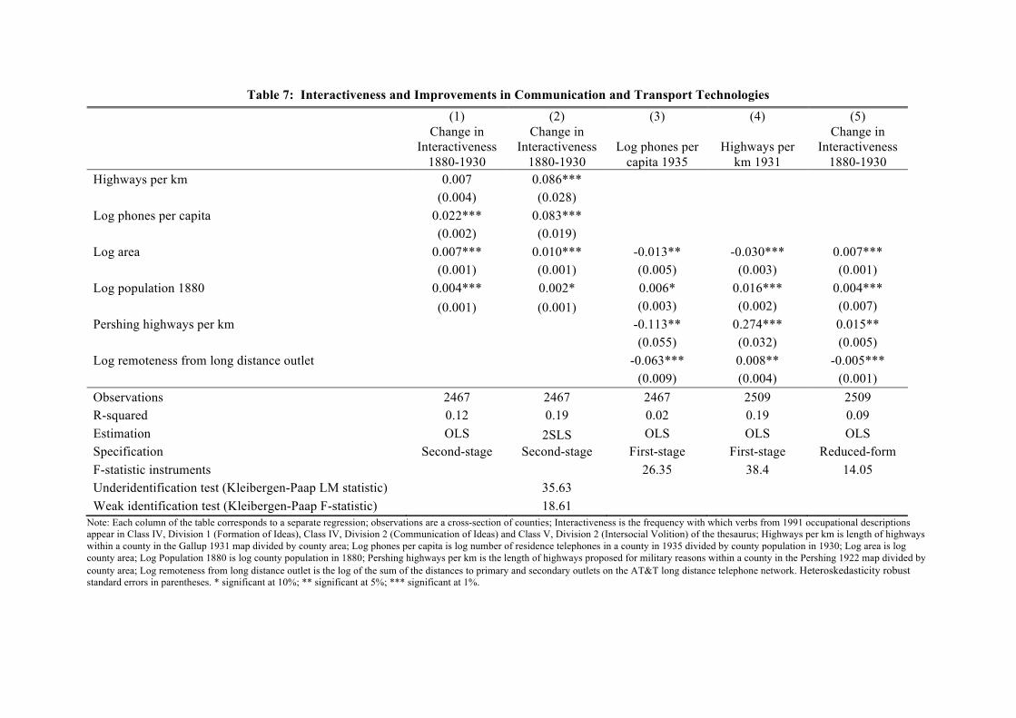
Table 7: Interactiveness and Improvements in Communication and Transport Technologies

Note: Each column of the table corresponds to a separate regression; observations are a cross-section of counties; Interactiveness is the frequency with which verbs from 1991 occupational descriptions appear in Class IV, Division 1 (Formation of Ideas), Class IV, Division 2 (Communication of Ideas) and Class V, Division 2 (Intersocial Volition) of the thesaurus; Highways per km is length of highways within a county in the Gallup 1931 map divided by county area; Log phones per capita is log number of residence telephones in a county in 1935 divided by county population in 1930; Log area is log county area; Log Population 1880 is log county population in 1880; Pershing highways per km is the length of highways proposed for military reasons within a county in the Pershing 1922 map divided by county area; Log remoteness from long distance outlet is the log of the sum of the distances to primary and secondary outlets on the AT&T long distance telephone network. Heteroskedasticity robust standard errors in parentheses. * significant at 10%; ** significant at 5%; *** significant at 1%.

(1) Change in

Interactiveness 1880-1930

(2) Change in

Interactiveness 1880-1930

(3)

Log phones per capita 1935

(4)

Highways per km 1931

(5) Change in

Interactiveness 1880-1930

Highways per km 0.007 0.086*** (0.004) (0.028) Log phones per capita 0.022*** 0.083*** (0.002) (0.019) Log area 0.007*** 0.010*** -0.013** -0.030*** 0.007***

(0.001) (0.001) (0.005) (0.003) (0.001) Log population 1880 0.004*** 0.002* 0.006* 0.016*** 0.004***

(0.001) (0.001) (0.003) (0.002) (0.007) Pershing highways per km -0.113** 0.274*** 0.015**

(0.055) (0.032) (0.005) Log remoteness from long distance outlet -0.063*** 0.008** -0.005***

(0.009) (0.004) (0.001) Observations 2467 2467 2467 2509 2509 R-squared 0.12 0.19 0.02 0.19 0.09 Estimation OLS 2SLS OLS OLS OLS Specification Second-stage Second-stage First-stage First-stage Reduced-form F-statistic instruments 26.35 38.4 14.05 Underidentification test (Kleibergen-Paap LM statistic) 35.63 Weak identification test (Kleibergen-Paap F-statistic) 18.61

.49

.51

.53

.55

.57

Inte

ract

iven

ess

1880 1900 1920 1940 1960 1980 2000Year

Overall Mean

Overall mean

.49

.51

.53

.55

.57

Inte

ract

iven

ess

1880 1900 1920 1940 1960 1980 2000Year

Metro Non-Metro

Mean by metro

Notes: Mean interactiveness is the employment-weighted average of interactiveness for each occupation. Interactiveness for eachoccupation is measured using the frequency with which verbs from time-invariant occupational descriptions from the 1991 DOTsappear in Class IV, Division 1 (Formation of Ideas), Class IV, Division 2 (Communication of Ideas) and Class V, Division 2 (Intersocial Volition)of the thesaurus.

Figure 1: Mean Interactiveness in Metro and Non-Metro Areas over Time

RIC, VA

ROC, NY

KCY, MO-KS

IND, IN

WOR, MA

NHV, CT

COL, OH

NOR, LA

LOU, KY/IN

PVD, MA/RIPBG, PA

SFR, CA

STL, MO-IL

DTR, MI CVL, OH BUF, NY

PHI, PA/NJ

CIN OH/KY/IN CHI, IL

NYC, CT/NY/NJ

BTM, MD

.495

.5.5

05.5

1.5

15

6 7 8 9 10

Panel A: 1880 MSAs

STC, PA

ROC, MN

TUS, AL

RMT, NC

TOP, KS

SFE, NM

RDG, CA

MUN, IN

NAS, NH

WCO, TX

MAN, NH

PCY, FL

RIC, WA

KOK, INSTC, MN

KAN, IL

MAN, OH

WIL, NC

HOU, LA

MON, LA

VIS, CA

RAC, WILCR, WI

JAC, TN

MER, CA

SAV, GA

NBD, MA

WOR, MA

GAD, AL

SLU, CA

UTI, NYHAT, MS

LIM, OH

SAL, CA

SBD, IN

SCR, CA

MED, OR

ROA, VA

GOL, NC

LAR, TX

OLY, WA

GTJ, CO

JAM, NY

SAL, OR

LNV, TX

LCR, NMOCA, FL

TAL, FL

ICY, IA

ODE, TX

MYR, SC

HAG, MD

GLE, NY

JOP, MO

KEN, WI

PTL, ME

NPL, FL

YOR, PA

SPR, MO

TRE, NJ

JAN, WI

LCH, LA

GRE, NC

SFD, CT

JAC, MI

JVL, NC

FLA, AZ-UT

RCK, ILLYN, VA

SHR, LA

SBA, CA

FLO, AL

LFY, IN

SPO, WA

DAN, VA

REN, NV

LUB, TX

FAR, ND/MN

DEC, ILRDG, PA

FIT, MA

SAG, MI

PRO, UT

STO, CA

PEO, IL

JON, PA

WIL, DE/NJ/MD

DOV, DE

NBU, NY

GRE, CO

FSM, AR/OK

YOU, OH-PA

LFA, LADOT, AL

WIC, KS

SRO, CA

MON, AL

LIN, NE

FWA, FL

EC, WI

MAC, GA

PEN, FL

NHV, CT

LEX, KY

DEC, AL

BRA, TX

VAL, CA

SAR, FL

MOD, CA

TOL, OH/MI

SPR, MA

GBA, WI

ELK, IN

SCR, PA

VTA, CA

FLI, MI

MCA, TX

CLA, TN/KY

JON, TN/VA

TUL, OKTXC, TXKIL, TX

GAI, FL

TAC, WASYR, NY

COL, MO

DUL, MN/WI

MEL, FL

MOB, AL

TUC, AZ

FCO, CO

DAN, CT

COL, GA/AL

HUN, AL

FPI, FL

MAD, WI

OMA, NE/IA

EVA, IN/KY

HAM, OH

HIC, NC

LAK, FL

JC, NJ

CHA, VA

CHI, CA

LAN, PA

PAL, FL

ERI, PA

LAN, MI

FAY, AR

JAC, MS

FAY, NC

DUT, NY

BOU, CO

KAL, MICC, TX

LR, AR

EUG, ORDAV, IL

BRY, TX

BLO, IN

FMY, FL

CHA, ILCED, IA

BIL, MT

ROC, NY

KNX, TN

RIC, VA

OKC, OK

PVD, MA/RI

BLO, IL

FWA, INBEN, MI

SLC, UT

BAR, MA

DM, IA

RAL, NC

HAR, PA

MEM, TN/AR/MS

BEL, WA

BRO, TX

DAY, FL

BRE, WA

LOU, KY/IN

SAT, TX

MON, NJ

NOR, LAAUB, AL

HAR, CT

MDX, NJ

BRO, MA

SAC, CA

LAW, MA/NH

ANN, AL

SJO, CA

NAS, TN

BER, NJ

ELP, TXFRE, CA

GRE, SC

BIN, NY

SFR, CA

LOW, MA/NH

HON, HITAM, FLORL, FL

CHA, TN/GA

NOR, VA

BRI, CT

PTL, OR

CAN, OH

MIL, WIJVL, FL

COL, CO

CHA,SC

COL, SC

OAK, CA

GTR, MI

STL, WA

ATH, GA

LV, NV

BIL, MS

PBG, PA

NAR, NJ

STL, MO-IL

SDG, CA

GAR, IN

BOI, ID

RIV, CA

BEA,TX

GRE, NC

MIA, FL

ALT, PA

KCY, MO-KS

IND, INASH, NCDAY, OH

PHX, AZ

NAS, NY

ALX, LA

DC, DC/MD/VA

FLA, FLMIN, MN

ORA, CA

ACY, NJ

AMA, TX

AUG, GA-SC

ANC, AK

BAK, CA

BIR, AL

Bat, LA

PHI, PA/NJ

APP, WI

COL, OH

BUF, NY

FWO, TXCIN OH/KY/IN

ALB, GA

DEN, CO

CHA, SC

.54

.55

.56

.57

.58

7 8 9 10 11

Panel B: 2000 MSAs

WOR, MANHV, CT

TOL, OH/MISCR, PA

SYR, NY

ROC, NY

RIC, VA

PVD, MA/RI

LOU, KY/IN

NOR, LA

SFR, CA

PBG, PA

STL, MO-IL

KCY, MO-KS

IND, IN

DC, DC/MD/VA

PHI, PA/NJ

COL, OH

BUF, NY

CIN OH/KY/IN

.55

.555

.56

.565

.57

.575

7 8 9 10 11 12

Panel C: 2000 MSAs, using only 1880 MSAs

Notes: X-axes are log population density. Y-axes are mean interactiveness. Mean interactiveness is the employment-weighted average ofinteractiveness for each occupation. Interactiveness for each occupation is measured using the frequency with which verbs from time-invariantoccupational descriptions from the 1991 DOTs appear in Class IV, Division 1 (Formation of Ideas), Class IV, Division 2 (Communicationof Ideas) and Class V, Division 2 (Intersocial Volition) of the thesaurus. Thick solid lines are the fitted values from locally-weightedlinear least squares regressions. Thin solid lines are 95 percent point confidence intervals. Figures (but not the regressions)are truncated at both ends for outliers.

Figure 2: Mean Interactiveness Across Metro Areas in 1880 and 2000

-.04

-.02

0.0

2.0

4.0

6

1900 1920 1940 1960 1980 2000

Clerical and Kindred

-.04

-.02

0.0

2.0

4.0

6

1900 1920 1940 1960 1980 2000

Craftsmen

-.04

-.02

0.0

2.0

4.0

6

1900 1920 1940 1960 1980 2000

Operatives

-.04

-.02

0.0

2.0

4.0

6

1900 1920 1940 1960 1980 2000

Sales Workers

-.04

-.02

0.0

2.0

4.0

6

1900 1920 1940 1960 1980 2000

Laborers

-.04

-.02

0.0

2.0

4.0

6

1900 1920 1940 1960 1980 2000

Service Workers

-.04

-.02

0.0

2.0

4.0

6

1900 1920 1940 1960 1980 2000

Managers

-.04

-.02

0.0

2.0

4.0

6

1900 1920 1940 1960 1980 2000

Professionals

Notes: Decomposition of the difference between mean and non-metro areas in the change in mean interactiveness over 20-year time periods(equation (25) in the paper) into the contributions of two-digit occupations. X-axes are 20-year differences. Y-axes are differences in the changein mean interactiveness between metro and non-metro areas. Mean interactiveness is the employment-weighted average of interactiveness foreach three-digit occupation. Interactiveness for each three-digit occupation is measured using the frequency with which verbs from time-invariantoccupational descriptions from the 1991 DOTs appear in Class IV, Division 1 (Formation of Ideas), Class IV, Division 2 (Communication of Ideas)and Class V, Division 2 (Intersocial Volition) of the thesaurus.

Figure 3: Decomposition of Difference in Change inInteractiveness Between Metro and Non-Metro Areas, Occupations

-.04

-.02

0.0

2.0

4

1900 1920 1940 1960 1980 2000

Manufacturing

-.04

-.02

0.0

2.0

4

1900 1920 1940 1960 1980 2000

Mining

-.04

-.02

0.0

2.0

4

1900 1920 1940 1960 1980 2000

Public Admin

-.04

-.02

0.0

2.0

4

1900 1920 1940 1960 1980 2000

Finance

-.04

-.02

0.0

2.0

4

1900 1920 1940 1960 1980 2000

Transportation-.0

4-.0

20

.02

.04

1900 1920 1940 1960 1980 2000

Entertainment

-.04

-.02

0.0

2.0

4

1900 1920 1940 1960 1980 2000

Trade

-.04

-.02

0.0

2.0

4

1900 1920 1940 1960 1980 2000

Construction

-.04

-.02

0.0

2.0

4

1900 1920 1940 1960 1980 2000

Business

-.04

-.02

0.0

2.0

4

1900 1920 1940 1960 1980 2000

Personal

-.04

-.02

0.0

2.0

4

1900 1920 1940 1960 1980 2000

Professional

Notes: Decomposition of the difference between mean and non-metro areas in the change in mean interactiveness over 20-year time periods(equation (25) in the paper) into the contributions of two-digit sectors. X-axes are 20-year differences. Y-axes are differences in the changein mean interactiveness between metro and non-metro areas. Mean interactiveness is the employment-weighted average of interactiveness foreach three-digit occupation. Interactiveness for each three-digit occupation is measured using the frequency with which verbs from time-invariantoccupational descriptions from the 1991 DOTs appear in Class IV, Division 1 (Formation of Ideas), Class IV, Division 2 (Communication of Ideas)and Class V, Division 2 (Intersocial Volition) of the thesaurus.

Figure 4: Decomposition of Difference in Change inInteractiveness Between Metro and Non-Metro Areas, Sectors