Solvency II: Principi e modelli per il ... - sia-attuari.it · Milano, 11 ottobre 2012 Solvency II: Principi e modelli per il calcolo del rischio nell’assicurazione vita

Milano, 11 ottobre 2012

Solvency II: Principi e modelli per il calcolo del rischio nell’assicurazione vita

2AGENDA

Solvency II Framework

1. An Introduction to Solvency II

2. Solvency 2 Definitions: Available Capital and Cap ital Requirement

3. Best Estimate of Liabilities: calculation process and examples

4. Required Capital: calculation process and example s

5. Applying Solvency II models: Risk Drivers and Pra ctical Examples

6. New Products and Capital Absorption: definitions and examples

3AGENDA




3. Best Estimate of Liabilities: calculations proces s and examples

4. Required Capital: calculations process and exampl es



4

We are defining rules to ensure the financial stability of an insurance and reinsurancecompany

1. adequacy of technical provisions to meet insurance obligations towardsthe policyholders;

2. availability of eligible and sufficient assets to cover the technicalprovisions;

3. respect of a minimum capital adequacy requirement (SCR)

Where are we?

An Introduction to Solvency 2

1. Calculation of the SH capital invested in the company (available capital)

2. Calculation of the capital requirement3. Verify that Available Capital > Capital Requirement

5

Current EU rule: “Solvency 1”

Where are we?

Available Capital = Net Asset Value (local GAAP) + adjustments for assets eligibility

Capital Requirement = 1. 4% x Reserves = “measuring the financial risks”2. 0.3% x Sum at Risk = “measuring the demographic risk s”

Next Future: “Solvency 2”

Available Capital = Net Asset Value (based on the market evaluation of assets and liabilities)

Capital Requirement (SCR) = The capital requirement is based on the market evaluation of assets and liabilities, consid ering the effective risks which the undertakings are exposed to


6Solvency II DirectiveSolvency II is based on a three pillars approach:

Pillar ICapital Requirements

• Assets and Liabilities Valuation (market consistent)

• Available Capital / Own Funds: Tier 1, Tier 2, Tier 3

• Capital Requirements:• Solvency Capital

Requirement (SCR)• Minimum Capital

Requirement (MCR)

SOLVENCY II FRAMEWORK

Pillar IISupervisory Review

• Supervisory power and processes

• Capital add-ons• Pillar II dampener

• Corporate Governance• Risk Management• Internal Audit• Actuarial functions• Compliance

• ORSA (Own Risk and Solvency Assessment)

Pillar IIIDisclosure Requirements

• Report to the market

• Report to the Supervisory Authority

«CALCULATIONS & NUMBERS»

Fomal Requirement to enhance the real «Risk

Management»

ReportingConsistency between

pillars and system


7Solvency II timeline

Local regulation towards

Solvency II i.e.Reg. 20 ISVAP,

MaRisk Germany,…

Dec 2009

22 Apr 2009:Solvency II Directive approved

31st Dec 2012*

Dec 2011

Dec 2010

Solvency II adoption

Nov 2009:Stress Tests

EIOPA

Jan 2010 EIOPA proposes Level 2

Directive

31 Jul 10: deadline for ISVAP for Internal Model

Draft of Level 2 Directive

Dec 2011 Level 3 (EIOPA)

Oct 2011: Level 2 Directive approved(European

Commission)

17 Dec 2009:Solvency II Directive published (Level 1)

QIS5

(*) The European Commission is considering the prop osal of postponing the date of entry into force of the Directive from 31 October 2012 to 31 December 2 012.

OMNIBUS 2

Potential delay

2015?


8AGENDA








9Methodology: Available Capital

Available Capital under Economic Balance Sheet

• Available Capital is the difference between the fair value of assets and the fair value of all liabilities

• Fair Value of Insurance Liabilities is estimated by projecting and discounting all future cash flows on a market consistent basis. It has two components: the Best Estimate Liability (BEL) and the Risk Margin.

– BEL is based on market values where they exist, and on estimates of market values where they do not exist (mark to model approach)

– Risk Margin reflects the margin required over BEL for situations where market prices cannot be observed, and is calculated using a cost of capital approach.

– Fair Value of Liabilities also includes the deferred tax liability from tax on profits that are expected to emerge on the difference between fair values and fiscal values of assets and liabilities.

Available Capital

BestEstimate

ofLiabilities

Risk Margin

Market value of assets

Available

Capital

Fair Value

of

Liabilities

Solvency 2 Definitions: Available Capital and Capit al Requirement

10

Risk Capital

Probability

ValueExpectedValue

Worst CaseValue

• Risk Capital is equal to the difference between

Available Capital (expected value) and Available

Capital (worst case value) after the “worst-case

scenario” (1-year value at risk approach, at a confidence

level consistent with the risk appetite)

• The mentioned “worst-case scenario” is referring to the

joint occurrence of negative outcomes of the different risks

Distribution of Available CapitalTotal Balance Sheet Approach

Available Capital

BestEstimate

ofLiabilities

Risk MarginMarket value of assets

Risk Capital

under Economic

Balance Sheet

Risk Capital (SCR) is the capital necessary to absorb the maximum loss of Available

Capital, identified according to a 1-year value at risk approach, at a specified confidence

level consistent with the risk appetite : at 99.5% (BBB) for Solvency II purposes.

Methodology: Risk Capital

AVAILABLE CAPITAL

FAIR VALUE OF

LIABILITIES

Solvency 2 Definitions: Available Capital and Capit al Requirement

11AGENDA








12Methodology: Available Capital

Available Capital under Economic Balance Sheet

• Available Capital is the difference between the fair value of assets and the fair value of all liabilities

• Fair Value of Insurance Liabilities is estimated by projecting and discounting all future cash flows on a market consistent basis. It has two components: the Best Estimate Liability (BEL) and the Risk Margin.

– BEL is based on market values where they exist, and on estimates of market values where they do not exist (mark to model approach)

– Risk Margin reflects the margin required over BEL for situations where market prices cannot be observed, and is calculated using a cost of capital approach.

– Fair Value of Liabilities also includes the deferred tax liability from tax on profits that are expected to emerge on the difference between fair values and fiscal values of assets and liabilities.

Available Capital

BestEstimate

ofLiabilities

Risk Margin

Market value of assets

Available

Capital

Fair Value

of

Liabilities

Best Estimate of Liabilities: calculations process and examples

13BEL = Present Value of Net Cash Flows


14BEL: Assets Projection


15BEL: Asset and Liabilities Projection


16BEL: Methodological Aspects

TP.1.213. Future cash-flows also need to be split into guaranteed anddiscretionary benefits because, as stated in Article 108 of the Level 1 text,the loss absorbing capacity of technical provisions is limited by thetechnical provisions relating to the future discretionary benefits. The riskmitigation effect provided by future discretionary benefits shall be nohigher than the sum of technical provisions and deferred taxes relating tothose future discretionary benefits.

BEL = Minimum guaranteed provisions + Future Discr etionary benefits (FDB )

FDB = BEL - Minimum guaranteed provisions

Future Cash Flows and Best Estimate Breakdown



Deterministic valuation where the revaluation of th e benefits is equal to the minimum guaranteed rate of return

How to calculate the minimum guarantee provisions


18Methodology: Understanding the FDB

Best Estimate of Liabilities

T+1Expense

T+2Expense

T+3Expense + Maturity Benefit

Avg yearly accrual 3.6%

MinimumGuarantee

FDB

MinimumGuarantee

FDB

FDB = BEL - Minimum guaranteed provisions

Min Gar 2%

Example:Premium = 100minimum guarantee for maturity benefits = 2%profit sharing = 60%Revaluation = max (2%, 60% x investment return)

• Projected Return on Asset = 6%

• Yearly revaluation= max (2%; 60% x 6%) = 3.6%

• Maturity Payment= 100 x (1+ 3.6%)^3 = 111

• Minimum Gurantee Benefit= 100 x (1 + 2%)^3 = 106

• FDB = 111 – 106 = 5



2.2.3.1 Definition of “best estimate” and allowance for uncertaintyTP.1.59. The best estimate shall correspond to the probability weighted average of future cash-flows

taking account of the time value of money, using the relevant risk-free interest rate termstructure.

TP.1.67. Valuation techniques considered to be appropriate actuarial and statistical methodologies tocalculate the best estimate as required by Article 86(a) include: simulation, deterministic andanalytical techniques (based on the distribution of future of cash-flows) or a combination thereof.

Present value of net cash-flows taking into conside ration embedded options, if exist

Is the “best estimate” a “good enough” estimate?



How the Embedded Options affects the BEL?

• Maturity Benefit before revaluation = 100


• Expected Return: 3 possible scenarios 0% - 5% - 10%

Deterministic (Traditional) Approach: Valuation in the Central Scenario:

Correct Approach:

return Unit Linked w/o guarantee Unit Linked 3% guar antee

5% 100 x (1 + 5%) = 105 100 x (1 + 5%) = 105

return Unit Linked w/o guarantee Unit Linked 3% guar antee

0% 100 x (1 + 0%) = 100 100 x (1 + 3%) = 103

5% 100 x (1 + 5%) = 105 100 x (1 + 5%) = 105

10% 100 x (1 + 10%) = 110 100 x (1 + 10%) = 110

avg (100+105+110) / 3 = 105 (103+105+110) / 3 = 106

Average of the valuation in all the scenarios

• For Unit Linked w/o guarantee: BEL (centrale) = average BEL (in all the scenarios)

• For Unit Linked with guarantee: BEL (centrale) < average BEL (in all the scenarios)

106 – 105 = 1 is the cost of the guarantee


-3,50%

-1,50%

0,50%

2,50%

4,50%

6,50%

8,50%

-3,50%

-1,50%

0,50%

2,50%

4,50%

6,50%

8,50%

CONTRACT W/O GUARANTEE YEARLY GUARANTEE «OUT OF THE MONEY»

Central (no gar) = AVG1000scen Central < AVG1000scen

Asymmetries:CE < AVG1000scen

C.E. curveStochastic scenariosMin Gar

The guarantee is out of the money:• CE = CE(no gar)• Cost of the Guarantee = CE - AVG1000scen

For product without guarantee CE = AVG1000scenNo need for stochastic scenarios.



YEARLY GUARANTEE «IN THE MONEY»

Central < AVG1000scen Central < AVG1000scen

C.E. curveStochastic scenariosMin Gar

The guarantee is out of the money:• CE = CE(no gar)• Cost of the Guarantee = CE - AVG1000scen

-3,50%

-1,50%

0,50%

2,50%

4,50%

6,50%

8,50%

The guarantee is «in the money»:• CE < CE(no gar)• Cost of the Guarantee :

Intrinsic Value = CE – CE(no gar) + Time Value = AVG1000scen – CE

AT MATURITY GUARANTEE

0%

50%

100%

150%

200%

250%

Asymmetries:CE <

AVG1000scen

Asymmetries:CE < AVG1000scen

«in the money»CE > CE(no gar)

Reserves in the C.E. curveReserves in the stochastic scenariosReserves at the minimum guarantee



1. Deterministic approach: for business where cash flows do not depend on, or move linearlywith market movements (i.e. business not characterised by asymmetries in shareholder’sresults), the calculation can be performed using the certainty equivalent approach.� Definition of a central scenario to project assets and liabilities and to discount the cash

flows

2. Analytic Approach: In case of business where the cash flows generated by the financialoptions can be easily separated from the underlying liability (e.g. some unit-linked products),closed form solutions may be appropriate.� Deterministic valuation of the product ignoring the financial options� Closed form solutions to determine the value of the financial options (e.g. Black-Scholes

formula)� It does not allow for any policyholder or management actions.

BEL Calculation: different approaches for different liabi lities

Contracts w/o profit sharing and guarantees

Contracts with “simple” financial options



3.Stochastic simulation approach : for business where cash-flows contain options andfinancial guarantees, characterised by asymmetric relationship between assets and liabilities,e.g. traditional participating business

� Availability of Actuarial Tool to project future cash flows of assets and liabilities (ALM view),which is able to run a full set of economic scenarios, tacking into consideration managementrules and policyholder behaviour

� Availability of Application Tool to generate stochastic scenarios for projections of asset pricesand returns

Contracts with guarantee and profit sharing


25Market Consistent Valuation

A valuation algorithm is a method for converting projected cash flows into a present value.A valuation is market consistent if it replicates the market prices of the assets.

The natural method of valuing such assets (or liabilities) would be to calculate the expectedvalue of present value of future cash flows

future cash flows at time t

discount factor

The calculation of expected value requires a probability distribution

There are two ways of valuing cash flows which must produce equivalent values under themodern financial economic theory:

� discount cash flows at the reference risk rate using risk-neutral probabilities

� consider real world probabilities discounting cash flows with the use of risk-adjusted rate (deflator)



Arbitrage-free pricing is the foundation for the basis of financial theory and pricing

If two assets yield the same set of future cash flows, they must have the same price in themarket otherwise a risk-free profit (arbitrage opportunity) could be made by takingappropriate positions in the underlying assets

What is the forward price agreed today of an equity in 1 year ha ving:

S = Equity price = 100g = Expected equity yield = 7%r = Risk-free growth rate = 3%

i. S*(1+g)/(1+r) = 100*1.07/1.03 = 103.88

ii. S*(1+r) = 100*1.03= 103

Contract

i ii

Forward Sell Sell

Buy one share -100.00 -100.00

Borrow 100 at risk free 100.00 100.00

Forward price receipts 103.88 103.00

Repay borrowings 103.00 103.00

Net cash flow 0.88 0.00

Answer


27Market Consistent Valuation – Risk Neutral

One of the major consequences of the Black and Scholes result is that the value of anoption does not depend on the risk preferences of the investor

From the other side, as the risk preferences of investors do not affect the value of theoption, any equity risk premium is irrelevant

In the risk neutral valuation

� the expected excess return over the risk reference rate is zero for all the assets

� interest rate used to discount future cash flows is the reference risk rate

� As consequence, the probability are calibrated to the market

time 0

Scenario 1 Scenario 2 Expected return

Reference rate 3% 3%

Equity price 100 115 95 3%

Bond 100 103 103 3%

Probability 40% 60%

time 1


28Market Consistent Valuation – Real World

In the real world investors are not risk neutral and risk premiums are a fact of life ininvestment decisions which themselves affect the performance of assets.

Moving from a risk-neutral to real world

� The return of the assets changes, reflecting the risk premiums of investors for assetswith different risk characteristics and this happen in tandem with the use of the realprobability distribution of return

� To produce a market consistent valuation, the reference rate can no longer be used anda risk-adjusted rate for each scenario (deflator) has to be derived

time 0

Scenario 1 Scenario 2 Expected return

Deflator 86.3% 105.9%

Equity price 100 115 95 4%

Bond 100 103 103 3%

Probability 45% 55%

time 1



In the Risk Neutral Environment, setting the risk free rates has always 2 effects on thecalculation of the Best Estimate of the Liabilities:


A: It defines the “discount factors”

Increasing the risk free rates, increase the discount factors,

decrasing the BEL


In the Risk Neutral Environment, setting the risk free rates has always 2 effects on thecalculation of the Best Estimate of the Liabilities:


B: It defines the average expected return on the assets

Increasing the risk free rates, increases the projected

returns, increasing the BEL

31Why Economic Scenario Generators?

The financial products sold by insurance companies often contain guarantees and optionsof numerous varieties, (i.e. maturity guarantee, multi-period guarantees)

At the time of policy initiation, the options embedded in insurance contracts were so far out-of-the-money, that the companies disregarded their value as it was considered negligiblecompared with the costs associated with the valuation.

In light of current economic events and new legislations, insurance companies haverealised the importance of properly managing their options and guarantees and it is one ofthe most challenging problems faced by insurance companies today.


32Economic Scenario Generators

0

1

2

3

4

5

0 10 20 30 40

Real world Real world

• reflect the expected future evolution of the economy by the insurance company (reflect the real world, hence the name)

• include risk premium • calibration of volatilities is usually

based on analysis of historical data

Economic Scenario

Market consistentMarket consistent

• reproduce market prices• risk neutral, i.e. they do not include risk

premium• calibration of volatilities is usually

based on implied market data• arbitrage free

Interest

Rate

Interest

Rate

Equity

Real

Estate

Real

Estate

Real

Yield

Real

Yield

Credit


33Economic Scenario Generators – Interest rate models

Short rate : based on instantaneous short rate� Equilibrium or endogenous term structure

term structure of interest rate in an outputVasicek (1977), Dothan (1978), Cox-Ingersoll-Ross (1985)

� No-arbitragematch the term structure of interest rateHull-White (1990)

Black-Karasinski (1991)

� Forward rate : based on instantaneous forward rateinstantaneous forward Heath-Jarrow-Morton (1992)

� LIBOR and swap market : describe the evolution of rates directly observable in the market

Instantaneous rate

not observable in

the market

Arbitrage free, are

perfect for market

consistent valuation

Easy to calibrate

The interest rate model is a central part of the ESG, as the price of most of the financialinstruments are related to interest rates.A large number of models have been developed in the few decades:

Good pricing only

for atm asset

Good pricing only

for all assets

Hard to calibrate



Considering interest rate models where the market yield curve is a direct input, it ispossible to derive an excellent-fitting model yield curve (the delta are reallyunimportant).



The calibration of the volatility of the term structure is based on swaption prices, sincethese instruments gives the holder the right, but not the obligation, to enter an interestrate swap at a given future date, the maturity date of the swaption


36Economic Scenario Generators – Credit model Calibrat ion

The most used Credit model is the Jarrow, Lando and Turnbull (1997) that is able to

� fit market credit spread for each rating class matching a single spread of agiven rating and maturity

� provide a risk-neutral probability through annual transition matrix movingbonds to a different rating class (including default)

AAA AA A BBB BB B CCC D

AAA 90.0% 8.0% 1.0% 0.5% 0.3% 0.2% 0.0% 0.0%

AA 2.0% 86.0% 3.0% 2.5% 2.3% 2.2% 1.6% 0.4%

A 1.5% 2.0% 84.0% 5.0% 2.8% 2.4% 1.8% 0.5%

BBB 0.4% 1.8% 2.5% 81.0% 4.0% 3.2% 4.0% 3.1%

BB 0.3% 1.2% 1.3% 7.0% 78.0% 3.5% 4.5% 4.2%

B 0.2% 0.3% 0.5% 2.5% 4.0% 75.0% 5.0% 12.5%

CCC 0.1% 0.2% 0.4% 1.4% 2.0% 3.0% 71.0% 21.9%

D 0.0% 0.0% 0.0% 0.0% 0.0% 0.0% 0.0% 100.0%

Rating at End of Period

Ra

tin

g a

t st

art

of

pe

rio

d


37Economic Scenario Generators – Equity model Calibrat ion

Equity models are calibrated to equity implied volatilities, that are generally traded withterms up to two years; long terms are available over-the-counter (OTC) frominvestment bank. The choice depends on the users’ appetite for sophistication andliability profile

Constant volatility

(CV)

is the Black-Scholes log-normalmodel implied volatilities of optionswill be quite invariant with respect tooption term and strike.

Time varying deterministic volatility

(TVDV)

volatility vary by time accordingmonotonic deterministic functionIt captures the term structure ofimplied volatilities but are stillinvariant by strike

Stochastic volatility jump diffusion (SVJD)

captures the term structure and thevolatility skew


38Economic Scenario Generators – Reduce Sampling Error

The Monte Carlo technique is subject to statistical error (“sampling error”); to reducethe magnitude of sampling error it is possible to

� Run more simulation : the size of sampling error scales with the square root of thenumber of simulations. This mean that we would need to run 4 times the number ofscenarios to halve the sampling error.

� Variance reduction techniques : “adjust” the simulations, or the cash flowsproduced by them, or the weights assigned to them in a way that ensures theresulting valuations are still “valid” but the sampling error is reduced.

Martingale test is performed verifying that the discounted prices of the asset is thesame as today’s price

Equity Risk free Deflator PV Equity Equity Risk free Deflator PV Equity

0 1.00 0 1.00

1 1.05 5% 95.24% 1.00 1 1.03 3% 97.09% 1.00

2 1.10 5% 90.70% 1.00 2 1.06 3% 94.26% 1.00

3 1.17 5% 86.38% 1.01 3 1.11 3% 91.51% 1.01

4 1.23 5% 82.27% 1.01 4 1.13 3% 88.85% 1.01

5 1.29 5% 78.35% 1.01 5 1.17 3% 86.26% 1.01

6 1.35 5% 74.62% 1.01 6 1.21 3% 83.75% 1.01

7 1.42 5% 71.07% 1.01 7 1.24 3% 81.31% 1.01

8 1.49 5% 67.68% 1.01 8 1.28 3% 78.94% 1.01

9 1.58 5% 64.46% 1.02 9 1.33 3% 76.64% 1.02

10 1.66 5% 61.39% 1.02 10 1.37 3% 74.41% 1.02


39Economic Scenario Generators – How Many simulations?

Martingale test is so used to determine how many simulations are to be considered inthe calibration of Economic Scenario.


40Valuation Framework “the story so far”

The “Market Consistency”

The calculation of technical provisions should be consistent with the valuation of assets and other liabilities, market consistent and in line with international developments in accounting and supervision.

The Solvency 2 directive prescribes that:

The CFO Forum in 2008 defines market consistent

principles for the Embedded Vale Calculation


41CFO Forum and MCEV Principles

� In May 2004, the CFO Forum published the European Embedded Value Principles and member companies agreed to adopt EEVP from 2006 (with reference to 2005 financial year)

� EEV Principles consisted of 12 Principles and65 related areas of Guidance

� Other 127 comments, collected in the “Basis for Conclusions”, summarised the considerations in producing the Principles and Guidance

� In October 2005, additional guidance on EEV disclosures was published to improve consistency of disclosures and sensitivities



European Embedded Value Principles

�� Principle 1 Introduction

�� Principle 2 Coverage

�� Principle 3 EV Definitions

�� Principle 4 Free Surplus

�� Principle 5 Required capital

�� Principle 6 Future shareholder cash flow from the in-force covered business

�� Principle 7 Financial options and

guarantees

�� Principle 8 New Business and renewals

�� Principle 9 Assessment of appropriate projection assumptions

�� Principle 10 Economic assumptions

�� Principle 11 Participating business

�� Principle 12 Disclosure

Required use of appropriate approaches ( e.g. stochastic simulations) to determine the impact of financial guarantees



CFO Forum – June 2008: launch of MCEV Principles

On the 4th June 2008, the CFO published the Market Consistent Embedded Value

Principles

MCEV Principles:

� replaced the EEV Principles (i.e. standalone document, no t supplement to EEV)

� at beginning compulsory from year-end 2009 for CFO Forum members(early adoption was possible)

� mandated independent external reviewof results as well as methodology and assumptions



Financial Options and

Guarantees

�� Principle 7

Frictional Costs of Required Capital

�� Principle 8

Required Capital�� Principle 5

Value of in-force Covered Business

�� Principle 6

�� Principle 9

�� Principle 4

�� Principle 3

�� Principle 2

�� Principle 1

Cost of Residual Non Headgeable Risks

Free Surplus

MCEV Definitions

Coverage

Introduction

Financial Options and

Guarantees

�� Principle 7

Frictional Costs of Required Capital

�� Principle 8

Required Capital�� Principle 5

Value of in-force Covered Business

�� Principle 6

�� Principle 9

�� Principle 4

�� Principle 3

�� Principle 2

�� Principle 1

Cost of Residual Non Headgeable Risks

Free Surplus

MCEV Definitions

Coverage

Introduction

Stochastic models�� Principle 15

Investment Returns and Discount Rates

�� Principle 13

Reference Rates�� Principle 14

�� Principle 17

�� Principle 16

�� Principle 12

�� Principle 11

�� Principle 10

Disclosure

Participating business

Economic Assumptions

Assessment of Appropriate Non Economic Projection Assumptions

New Business and

Renewals

Stochastic models�� Principle 15

Investment Returns and Discount Rates

�� Principle 13

Reference Rates�� Principle 14

�� Principle 17

�� Principle 16

�� Principle 12

�� Principle 11

�� Principle 10

Disclosure

Participating business

Economic Assumptions

Assessment of Appropriate Non Economic Projection Assumptions

New Business and

Renewals

Market Consistent Embedded Value Principles



The launch of MCEV Principles was initially welcomed by analysts and investor community and it was seen as a step in the right direction

Main implications of the MCEV Principles:

�all projected cash flows should be valued in line with the price of similar cash flows that are traded in the capital markets [Principle 3 & 7]

�use of swap rates as reference rates (i.e. proxy for risk-free rate) [Principle 14]

�no adjustment for liquidity premium is allowed [Principle 14]

�volatility assumptions should be based on implied volatilities derived from the market as at the valuation date (rather than based on historic volatilities) [Principle 15]

� required capital should include amounts required to meet internal objectives (based on internal risk assessment or targeted credit rating) [Principle 5]

�explicit and separate allowance for the cost of non hedgeable risks [Principle 9]


46Financial market situation at YE2008: a “dislocated ” market

Par Rate EUR (Swap) vs Par Rate ITA (Govt) - YE2008

1.00%

2.00%

3.00%

4.00%

5.00%

6.00%

1 2 3 4 5 6 7 8 9 10 11 12 13 14 15 16 17 18 19 20 21 22 23 24 25 26 27 28 29 30

EUR (swap) ITA (govt)

Average ∆ (Swap - Govt) -0.94%

For Italy government bond rates higher than swap ra tes


47CFO Forum - December 2008: tackling extreme financia l


48CFO Forum - May 2009: deferral of mandatory date

CFO Forum statement• further work needed• mandatory date of MCEV Principles

reporting deferred from 2009 to 2011


49CFO Forum - October 2009: amendment of MCEV principl es

In October 2009, the CFO Forum announced a change to its MCEV Principles to reflect the inclusion of a liquidity premium


50Latest developments – YE2011 Tackling the sovereign debt crisis


51Latest developments – Setting the Risk Free Rates

The risk-free rate term structure is one of the most critical areas of Solvency2 framework, for the

Fair Value of Liabilities and Available Capital.

The European Commission has defined in the QIS5 TS the risk free rate as

«SWAP – 10 bps + ILLIQUIDITY PREMIUM * %bucket»

BUT

The recent volatility in the financial market requests a «predictable counter-cyclical mechanism»

to reduce the volatility without producing other undesirable effects.

Without a predictable counter-cyclical mechanism, insurers will be faced with uncertainty in

managing risk which may lead to improper risk management (forced sale of assets and

inappropriate ALM).

Lots of proposal are under discussion. The following are the most relevant open issues:

• the basic risk-free interest rate term structure (including credit spread)

• a counter-cyclical premium (only where market is dislocated)

• a matching adjustment (only for specific products)

• an extrapolation model (including UFR and convergence speed).

In the Trialogue should be agreed an exhaustive package for LTG. An Impact Assessment should be

performed during next months


52Counter Cyclical Premium: when and how

The CCP should include

� an illiquidity premium (IP)

� a government spread premium (GSP)

Periods of distress will be independently identified by EITHER of these two triggers (Corporate bond

spread OR Sovereign bond spread).

When the CCP triggers are activeted, the risk free rate can be:

Risk Free = SWAP – credit adjustment + α * IP + β * GSP

GSP = f (AAA&Other, swap, AA,default)


53Counter Cyclical Premium: when and how

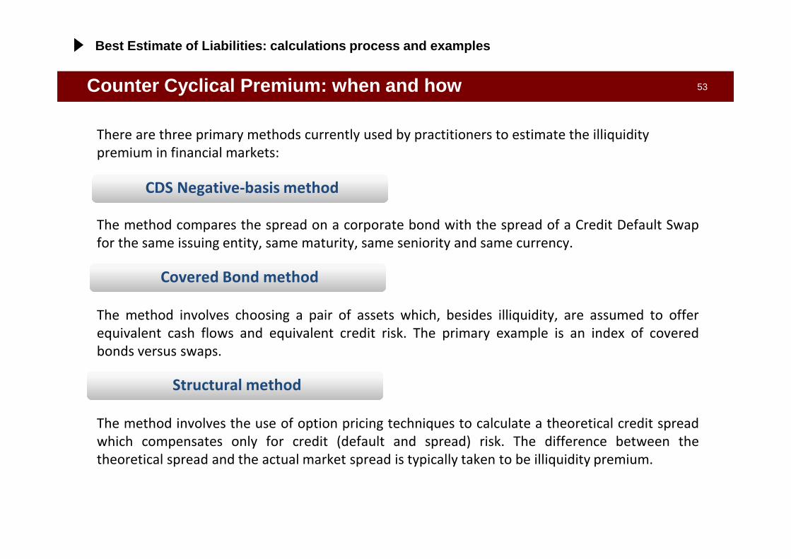
There are three primary methods currently used by practitioners to estimate the illiquidity

premium in financial markets:

The method compares the spread on a corporate bond with the spread of a Credit Default Swap

for the same issuing entity, same maturity, same seniority and same currency.

The method involves choosing a pair of assets which, besides illiquidity, are assumed to offer

equivalent cash flows and equivalent credit risk. The primary example is an index of covered

bonds versus swaps.

The method involves the use of option pricing techniques to calculate a theoretical credit spread

which compensates only for credit (default and spread) risk. The difference between the

theoretical spread and the actual market spread is typically taken to be illiquidity premium.

CDS Negative-basis method

Structural method

Covered Bond method


54Derivation of the illiquidity premium

By making use of estimates derived from a number of different methods together EIOPA

creates an overall estimate.

To do this a “proxy” method based on a simple transformation of the observed credit

spread is proposed:

The corporate bond spread is so considered to be comprised of three components:

� an allowance for the cost of default

� a risk premium to compensate bond

holders for bearing credit risk

� an illiquidity premium to compensate

for the costs and associated

uncertainty of trading illiquid bonds


55A practical example


CCP = (Govies Adj. ; Illiquidity) = 178 bps

56A simplified example (1/2)

Illiquidity Premium: what impact if asset allocation is 100% Government Bond ?The result depends on the rationale underlying spread widening

Illiquidity premium Govies Spread

CCP – Govies Spread Adjustment: what impact if asset allocation is 100% Basket of Government Bond?The result depends on the rationale underlying spread widening

Index Market Condition Asset Liabilities Own Fund Note6 Official YE2011 1.419 1.374 44 RF = swap rate + IP (118bps)7 Spread + 100 1.419 1.289 130 RF = swap rate + IP (118bps) +100bps8 Spread + 100 1.305 1.374 -69 RF = swap rate + IP (118bps)

Index Market Condition Asset Liabilities Own Fund Note9 Official YE2011 1.419 1.275 144 RF = swap rate + GSP (180bps)10 Spread + 100 1.394 1.252 142 RF = swap rate + GSP (180bps) + 21bps11 Spread + 100 1.305 1.177 128 RF = swap rate + GSP (180bps) + 100 bps

Basket SpreadBTP Spread Only


57A simplified example (2/2)

BTP spread Basket Spread with 459 bps BTP

CCP – Govies Spread Adjustment: what impact if asset allocation is 100% BTP ?The result depends on the rationale underlying spread widening

CCP – Govies Spread Adjustment: what impact if asset allocation is 100% BUND ?The result depends on the rationale underlying spread widening

Index Market Condition Asset Liabilities Own Fund Note12 Official YE2011 1.419 1.275 144 RF = swap rate + GSP (180bps)13 Spread + 100 1.305 1.252 53 RF = swap rate + GSP (180bps) + 21bps14 Spread + 100 898 1.177 -279 RF = swap rate + GSP (180bps) + 100 bps

Index Market Condition Asset Liabilities Own Fund Note15 Official YE2011 1.419 1.275 144 RF = swap rate + GSP (180bps)16 Spread + 100 1.419 1.252 167 RF = swap rate + GSP (180bps) + 21bps17 Spread + 100 1.419 1.177 242 RF = swap rate + GSP (180bps) + 100 bps

Basket Spread with 459 bps BTP

BTP spread


58Why a matching adjustment applied to a broader rang e of business?

�MA has been introduced in Omnibus II for a limited number of products only.

�European Insurance industry asks the application of MA to a broader range ofinsurance business since:

� Level playing field for all participants across Europe.� Avoids making own funds appear more volatile than they actually are.

Insurers can demonstrate that they mitigate spread risks (typically investing in assets heldto maturity) and are generally not exposed to forced sale of the corresponding assets. Thissubstantially eliminates the exposure of insurers to market movements.

THE MATCHING ADJUSMENT PROPOSAL CAPTURES AND ARTICU LATES IN PRINCIPLES THE UNDERLYING ECONOMICS DESCRIBED ABOVE

�Solvency2 should capture the real risks for insurers: proposed SII regime makesinsurance business more volatile than it really is.

�The inclusion of a MA removes the inclusion of risk to which the insurer is not exposed

�A Europe-wide application of a MA will promote stable long term investment and willsupport national governments and real economy through investment in sovereign bondsand long-term economic growth projects.


59Example: Italian Product (profit sharing via Segreg ated Fund)

Currently excluded because assets and liabilities are not fully matched

and underwriting risks other than expense and longevity risk exist


60Extrapolation – Smith Wilson Approach


61Extrapolation – From QIS5 to new industry proposal


62What does “best estimate operative assumptions” mea n?

Open issues

� Mortality and longevity: selection factor or/and future trend?

� Lapse: are the historical observations useful to infer the future?

� Lapse: what type of link between market and surrenders?

� Expense: is the S2 going concern?

� Expense: what type of inflation?


63Mortality assumptions – Lee Carter model

Lee Carter approach to mortality forecast takes into account a stochastic projection model both to

Best Estimate and Worst Case valuation

� Observed mortality rates are random variables representing past mortality

� Forecasted mortality rates are estimates of random variables representing future mortality

Mortality forecasts: BE and WC estimation

0.00%

0.01%

0.02%

0.03%

0.04%

0.05%

0.06%

0.07%

0.08%

1950 1960 1970 1980 1990 2000 2010 2020 2030 2040 2050 2060

Historic SIM Age 35 (BE) Age 35 (down) Age 35 (up)

Sample: observed from mortality

rates

A model linking the probabilistic structure of the stochastic process to

the sample

BE proj

WC up

WC down

Random paths of stochastic process


64Mortality assumptions – Lee Carter model Example (It aly)

Historical and projected mortality rates – q(x,t)


65Mortality assumptions – Selection factor

)(*)(Pr

,,hSh qq

oj

txtx=

The mortality in the various underwriting classes and product groups can be expected to differ from projected mortality rates

Major selection factor causes:

• Age and sex

• Smoker status

• Socioeconomic status

• Method and quality of underwriting

• Sales channel

• Types of product

∑

∑=

i

Ei

i

Ai

hDeath

hDeathhs

)(

)()(ˆ

)(*)( Pr, hExposuresqhDeath i

ojtx

Ei =


66Mortality assumptions – Selection factor

Application to real portfolioSelection factors from 1996 to 2010 grouped in bukets of ages Average selection factors for different age bukets

considering different periods


67Mortality assumptions – Local GAAP vs. Best Estimate

Term Life contract

Age 40

Term 10

I order mortality table SIM 2003

II order mortality table 80% SIM 2003

Technical interest 3%

Premium loading 10%

n. of contracts 1,000

Premium 213

Sum in case of death 100,000


68Impact of mortality improvement assumptions

Annual Premium - Individual Term Lifeportfolio

(23,200 policies)

One Model Point of AP IndividualTerm Life portfolio(7 policies – male – issue year 2007duration 15 years I order mortality table SIM1981)

EBS YE2011

valuation (1)

Mortality

Improvement ∆∆∆∆%

Local GAAP reserves 5.849,29 5.849,29

Best Estimate

BEL 8.824,29- 10.493,31- -19%

Worst Case at 99.5%

10% mortality stress

Lee Carter

stress

BEL 8.292,53- 9.396,68- -13%

RAC - Mortality trend 531,76 1.096,64 106%


BEL 7.761,25-

RAC - Mortality trend 1.063,04

EBS YE2011

Mortality

Improvement ∆∆∆∆%

Local GAAP reserves 32.377.899,40 32.377.899,40

Best Estimate

BEL 28.841.557,47- 36.340.271,13- -26%

Worst Case at 99.5%


Lee Carter

stress

BEL 24.864.107,31- 27.560.064,14- -11%

RAC - Mortality trend 3.977.450,16 8.780.206,99 121%


BEL 20.895.855,89-

RAC - Mortality trend 7.945.701,58


69AGENDA








70

Risk Capital

Probability

ValueExpectedValue

Worst CaseValue

• Risk Capital is equal to the difference between

Available Capital (expected value) and Available

Capital (worst case value) after the “worst-case

scenario” (1-year value at risk approach, at a confidence

level consistent with the risk appetite)

• The mentioned “worst-case scenario” is referring to the

joint occurrence of negative outcomes of the different risks

Distribution of Available CapitalTotal Balance Sheet Approach

Available Capital

BestEstimate

ofLiabilities

Risk MarginMarket value of assets

Risk Capital

under Economic

Balance Sheet

Risk Capital is the capital necessary to absorb the maximum loss of Available Capital,

identified according to a 1-year value at risk approach, at a specified confidence level

consistent with the risk appetite : at 99.5% (BBB) for Solvency II purposes.

Methodology: Risk Capital

AVAILABLE CAPITAL

FAIR VALUE OF

LIABILITIES

Required Capital: calculations process and examples

71Methodology for Risk Capital: Theoretical approach

Discounting to t=0 at risk free rate

Risk Capital

Probability

ValueExpected

Value0.50%

Worst CaseValue

Available Capital

EconomicBalance Sheet

at t=0

SolvencyBalance Sheet

at t=0

0 1 Time

AvailableCapital

Realistic simulation of the business over the first year

Market consistent revaluationof liabilities at t=1

Joint distribution of all the risk

factors

1.000 simulation for each realistic

simulation:10.000 x 1.000


72Methodology for Risk capital: Modular Approach (1/3 )

density f(x)

Markets

Credit Risk

Longevity

Mortality

Operating Events

LapsesExpenses

Identification of Risk Factors that affects theAC distribution

f(x)

Risk FactorBEWC

Focus on the single risk factors:for each of them the stress levelcorresponding to desired confidencelevel is determined

alternative solution: Modular approach

ACAC

Best Estimate Worst Case risk factor i

SCR = AC (BE) – AC(WCi)0 1 Time

AvailableCapital

Best Estimate

Worst case(risk factor i)


73

BE WC

RISK FACTOR 1

BE WC

RISK DRIVER nRISK FACTOR 2

BE WC. . . . . . .

1……. CorrRCn;3CorrRCn;2CorrRCn;1RCn

1……. ……. …….…….

1CorrRC3;2CorrRC3;1RC3

1CorrRC2;1RC2

1RC1

RCn…….RC3RC2RC1

1……. CorrRCn;3CorrRCn;2CorrRCn;1RCn

1……. ……. …….…….

1CorrRC3;2CorrRC3;1RC3

1CorrRC2;1RC2

1RC1

RCn…….RC3RC2RC1

crrxc

rxcRCRCCorrRCRC ••= ∑

The stress impacts for all the risk drivers are finallyaggregated using a correlation matrix in stressconditions

Methodology for Risk capital: Modular Approach (2/3 )


74

Solvency II Framework: risk overview

Methodology for Risk capital: Modular Approach (3/3 )


75QIS5 – Final Results


76Methodology: Risk Capital

Is the Standard Formula the unique way to evaluate SCR for Solvency2

purpose?

�� Solvency II framework allows Companies to adopt an Internal Model or

a Partial Internal Model.

BUT

Internal Model (IM) and Partial Internal Model (PIM) must beapproved!

To obtain the approval, Companies are required to demonstra tethat their IM / PIM verifies some Tests and Standards explicitlyreported in the Solvency II Directive.


77Methodology: Risk Capital

StatisticalQuality

Standard

CalibrationStandard

Data quality – Adequate, applicable and relevant act uarial and statistical tecniques –PDF based on current and credible information and r ealistic assumptions – Coverage

of all material risks – Inclusion of mitigation tecn iques and diversification effects

The Internal Model must provide policyholder and be neficiaries with the same level of protection equivalent to the Standard Formula della formula standard (i.e. VaR 99,5%)

UseTest

The Internal Model must be widely used in and plays an important role in the Company’s system of governance

ValidationStandard

DocumentationStandard

A regular model validation cycle must be put in pla ce that includes monitoring the performance of the Internal Model, reviewing the on -going appropriateness of its

specification and testing its results against exper ience

Company must document the design and operational de tails of the Internal Model, guaranteeing compliance with Directive articles 120 -124, with focus on theory,

assumptions, mathematical and empirical basis and c ircumstances for not working

Profit and Loss

Attribution

The Internal Model must identify the sources of pro fits and losses and must explain those sources in respect of categorisation of inter nal model risks and the Company’s

risk profile

External Modeland Data

All the above mentioned requirements must be consid ered also regarding the use of external model and data obtained from a 3rd party


78Other Risk Based Capital Models

Different approaches can be implemented to evaluate Risk based Capital

�VaR or Tail VaR*: Solvency 2 vs Swiss Solvency Test

�One year or multi-year?

�Modular approach ?

�Probability distribution forecast? Using which type of model?

�Including or not loss absorbency capability of liability ?

�Internal model or standard formula?

*Value at Risk (VaR): massima perdita attesa, in uno specifico orizzonte temporale e ad un predefinito livello di confidenza.

TailVaR: media delle perdite che eccedono, in uno specifico orizzonte temporale un predefinito livello di confidenza.

Riassumendo, considerando 10.000 perdite simulate, il VaR sarà uguale alla 50-esima maggiore perdita mentre il TAilVAR

sarà la media delle 50 perdite maggiori.


79

Solvency II Framework: Underwriting Risk

Methodology for Risk capital: Underwriting Risk


80

Generali Group

Valuation Framework for Underwriting Risks

Available Capital: Pre Stress

Asset Liabilities

AvailableCapital

Available Capital: Post Stress

Pre Stress Post Stress

AvailableCapital

AvailableCapital

SCR

Risk Capital: ∆ Available Capital

� Calculation of MarketValue of the Assets andFair Value of theLiabilities in the CentralScenario with BestEstimate Assumptions

� Definition of the stressedunderwriting stressedfinancial assumptions

� Calculation of the BestEstiamate of theLiabilities in the stressedscenario

� Calculation of the SCR asthe difference betweenthe Available capital inthe central and in thestressed scenario

Stress

Asset Liabilities

AvailableCapital

Underwriting Risk


LONGEVITY RISK – annuity contracts

Change of Mortality Assumptions

Fair Value of Liabilities

1. Before Stress

2. After Stress


T+1Annuity

T+2Annuity

T+3Annuity

T+4Annuity

T+5Annuity

T+1Annuity

T+2Annuity

T+3Annuity

T+4Annuity

T+5Annuity

T+6Annuity

Mortality assumptions = qx (1- 25%)

Underwriting Risk


82

Solvency II Framework: Underwriting Risk

Methodology for Risk capital: Market Risk


Valuation Framework for Market and Credit Risks

Available Capital: Pre Stress

Asset Liabilities

AvailableCapital

Available Capital: Post Stress

Asset Liabilities

AvailableCapital

Stress


AvailableCapital

AvailableCapital

SCR

Risk Capital: ∆ Available Capital

� Calculation of MarketValue of the Assets andFair Value of theLiabilities in the CentralScenario with BestEstimate Assumptions

� Definition of the stressedfinancial stressedfinancial assumptions

� Calculation of the Marketvalue of the assets andthe Best Estimate of theLiabilities in the stressedscenario

� Calculation of the SCR asthe difference betweenthe Available capital inthe central and in thestressed scenario



Alternative definition of SCR: change in assets – change in liabilities

SCR = ∆ AC SCR = ∆ MVA - ∆ FVL

LAC “basic” interpretation and LAC index


AvailableCapital

AvailableCapital

SCR

Asset

SCR∆ MVA

∆ FVL

Liabilities

Asset

SCR

∆ MVA∆ FVL

Liabilities

SCR may be lower than ∆MVA,as the loss on the assets canbe partially “absorbed” by areduction of the Liabilities

LAC index =∆ Market value of Assets

∆ Fair value of Liabilities

� The SCR formula can berewritten as thedifference between thechange in market valueof the assets and thechange in market valueof the liabilities (pre andpost stress)

� This is the maininterpretation of theabsorbency capacity andit is applicable for Equity,Credit, Property andCurrency risks.



Equity Risk: Immediate loss in market value of the assets

1.Unit Linked Contract

∆ MVA

The benefits are constantlylinked to the return on theassets. The absorption isalmost «complete».LAC index = 90% - 95%

Asset Liabilities

SCR

∆ FVL

1. Before Stress 2. After Stress




850 BOND

150 EQUITY

950 FVL

50 AC

MV Equity - 33%= -50 850 BOND

100 EQUITY

903 FVL

47 AC

Change in Market Value = 50Change in Liabilities = 47SCR = AC – ACequity = 50 – 47 = 3Liability absorption = change in liabilities / chan ge in assets = 47/50 = 95%

Unit Linked Portfolio w/o Guarantee

• In a unit linked contract the market risk is in charge of the insured;• the asset stress produced only a “proportional reduction” of the expected profits(total MVAssets = -8% -> AC -8%)



2.Contract Without Profit Sharing

1. Before Stress 2. After Stress

SCR∆ MVA

No liability absorption.The SCR is equal to the lossin market value of the assets.LAC index = 0%

Asset Liabilities




Term Assurance

850 BOND

150 EQUITY

300 FVL

700 AC

MV Equity - 33%=-50 850 BOND

100 EQUITY

300 FVL

650 AC

• In a term the market risk is in charge of the insurer• the asset stress doesn’t affect the liabilities, therefore all the stress produces aPVFP reduction

Change in Market Value = 50Change in Liabilities= 0SCR = AC – ACequity = 50Liability absorption = change in liabilities / chan ge in assets = 0/50 = 0%



3.Traditional Saving contract minimum guarantee and pr ofit sharing


T+1Expense

T+2Expense


MinimumGuarantee

FDB


T+1Expense

T+2Expense


MinimumGuarantee

FDB

MinimumGuarantee

FDB

FDB

MinimumGuarantee

T+3Expense +

Maturity Benefit

T+3Expense +

Maturity Benefit




3.Traditional Saving contract minimum guarantee and pr ofit sharing

SCR

∆ MVA

The benefits are linked to thereturn on the assets. Theonly absorbing liability is theFDB.0% ≤ LAC index < 100%

Asset Liabilities

∆ FVL

Pre stress

MinimumGuarantee

FDBFDB

MinimumGuarantee

Post stressPre stress Post stress

Asset Liabilities

∆ MVA



91Methodology for Risk capital: Market Risk

850BONDCORP

150EQUITY

600 MinimumGuarantee

250AC

850BONDCORP

100EQUITY 240

AC

Change in Market value of Assets = 150*33% = 50Change in FVL = 750 – 710 = 40Change in AC = 250 – 240 = 10Liability absorption = 10/ 40 = 80%The loss is shared: 20% SH, 80% PH

Case C: Product with guarantee and Profit Sharing (80%)

• In a product with profit sharing, both proifts and losses are shared; the % ofsharing is a function of the portfolio structure and the level of the stress• In general we can notice an absence of linearity among the loss sharingpartecipation and the increase of the stress level

150 FDB

600 MinimumGuarantee

110 FDB

MV Equity - 33%=-50


92Methodology for Risk capital: Market Risk

1. the calculation of the market value of the assets and the fair value of the technical provisions at valuation date:

Equity Risk - The calculation process requires :

Fair Value Technical

Provisions:750

Market Value

Government Bonds: 450Corporate Bonds: 400Equities: 150

Asset Allocation

2. Calculation of the 99,5% stress on the asset side is calculated : i.e. the loss of 50 (150*33%).

3. re-valuation of the value of the technical provisions in the1,000 scenarios where the initial assets have a lower value (-50).The revaluation of benefits can be decreased according tothe profit sharing rules.

Fair Value of Tech.

Provisions:710

Loss on assets:

Tech. Provision decrease:

Capital requirement beforeabsorption:

Net capital requirement:

4. The capital requirement is not equal to 50 euro (as innon life segment) but 10 euro (50-40), by ceding part of theloss (80%) to the policyholders, through the absorptionprovided by the profit sharing rules.

Equity risk capital charge:

The liabilities absorption capability, depends on theexpected returns and on the level of the guarantees.

Corporate Bond

GovernmentBond

Equity

50

50

-40

10


Loss Absorbency Capacity – Equity Risk

Equity Risk: the LAC asymmetry

LAC vs change in expected returns

0,0%

20,0%

40,0%

60,0%

80,0%

100,0%

0,0% 0,5% 1,0% 1,5% 2,0% 2,5% 3,0% 3,5%

1.Profit

SharingEffect

2.Increased

Cost of the Guarantee

3.Exhaustionof the FDB

Sources of LAC asymmetry:




0,0%

20,0%

40,0%

60,0%

80,0%

100,0%

0,0% 0,5% 1,0% 1,5% 2,0% 2,5% 3,0% 3,5%

1.Profit

SharingEffect

2.Increased






1. Profit Sharing «mitigating» effect

MinimumGuarantee

FDB

Liabilities

Avg Return PH Return

6.5%

2.5%

2.7%

Gar = 2.5%

Bonus = 2.7%

PH = max(gar, 80% x return)

Asset

MinimumGuarantee

FDB

Liabilities


5.0%2.5%Gar = 2.5%

Bonus = 1.5%

Asset

∆ MVA-1.5%

1.5%-1.2%

-1.5%LAC = = 80% = Profit sharing

-1.2%

Before Stress

After Stress





0,0%

20,0%

40,0%

60,0%

80,0%

100,0%

0,0% 0,5% 1,0% 1,5% 2,0% 2,5% 3,0% 3,5%

1.Profit

SharingEffect

2.Increased



Risk Capital Calculation


2. Increased cost of the Guarantee

Cost of the guarantee

Cost of the guarantee 2.5%

1.5%

Liabilities

2.5%

2.2%

Liabilitiesw/o Guar

2.5%

3.0%

Liabilities Liabilitiesw/o Guar

2.5%

2.7%

Stochastic scenarios before stress

Stochastic scenarios after stress





0,0%

20,0%

40,0%

60,0%

80,0%

100,0%

0,0% 0,5% 1,0% 1,5% 2,0% 2,5% 3,0% 3,5%

1.Profit

SharingEffect

2.Increased


3.Exhaustion of the FDB



3. Exhaustion of the FDB


5.0%2.5%

Asset

∆ MVA-1.5%

1.5%-1.2%

-1.5%LAC = = 80%

-1.2%


2.5% 2.5%Asset

∆ MVA

-4.0%-2.7%

-4.0%LAC =

-2.7%


1.5% 2.5%Asset

∆ MVA

-5.0%-2.7%

-5.0%LAC =

-2.7%

= 67%

= 54%


100AGENDA








101Solvency 2 – Risk Optimization

Applying Solvency II models: Risk Drivers and Pract ical Examples

ASSETS

LIABILITIES

Asset management:

�Asset allocation based on effective risks Company want

to be exposed to

�Counterparty selection for monitoring credit and

concentration risks

Asset management:

�Asset allocation based on effective risks Company want

to be exposed to

�Counterparty selection for monitoring credit and

concentration risks

Product design and definition:

�Products generatingAvailable Capital

�Products allowing for liability absorbency

capacity

Product design and definition:

�Products generatingAvailable Capital

�Products allowing for liability absorbency

capacity

Under Solvency II perspective, risk optimization can be performed both on assets and

liabilities, considering also the impact on Available Capital and the dynamic interaction

between assets and liabilities .

102ORSA & SAA: A Segregated Fund Example

Applying Solvency II models: Risk Drivers and Pract ical Examples

SCR 244 SCR 135 SCR 218 SCR 287

103AGENDA








104New Products and Value

Products and Capital Absorption: definitions and ex amples

New Business Value = present value, at issue date, of future industrial profits (after taxesand reinsurance) expected to emerge from all contracts issued during the last

105New Products: Profit ratios based on «volumes»

New Business Margin (NBM) = NBV / APE = New Business Value/Annual Premium Equivalent (Regular premium+single premium/10)

� It is a multi-period profitability indicator

� Strength : widely used and easy to understand� Weaknesses : normalized assumption of 10 years of duration for single premiums

NBV/P.V. Premiums

� Expresses the profitability as a percentage of the products yearly turnover

� Strength : solves the problem of the normalization used in the NBM, representing the effective duration of the contract

= New Business Value/Present Value of Future Premiums

NBV/P. V. Reserves

�Expresses the profitability as a percentage of assets under management of the company related to the product under analysis

� Strength : is a good measure of the annual profitability in terms of managed assets� Weakness : meaningless for products where the mathematical reserve is a very small amount

(e.g. Pure risk products)

= New Business Value/Present Value of Future Premiums


106New Products: Profit ratios based on «volumes»

Profitability ratios based on volumes: which indicator should we look at?

� NBM: the less profitable is Product 1� the denominator is the same for the 3 products (equal to 1000) and hence increasing the term brings to higher

NBV that is reported to the same amount leading to a higher value of the ratio� the effect of the annual loss of the fee (0.15% between Products 1 and 3) is lower of the effect of gaining it for

a longer time

� NBV/PVP: the less profitable is Product 3� the denominator varies i.e. increases with the term; in Product 3 the NBV (the same as in the NBM) is divided

by a higher amount

� NBV/PVR: the less profitable is Product 3 but the most profitable is Product 1� this indicator rewards the product with higher management fee


107New Products: Profit Breakdown

� Gives indication on the equilibrium of the product among different sources of profits :

– What is the main source of profit of the product?– Is it highly exposed on the financial side?– Are the loadings sufficient to cover the expenses?


108New Products: Capital Absorption

� In a Solvency II perspective, when a new product is launched, it shall be evaluated in terms of

capital absorption and remuneration

� Estimate of the SCR at product level, possibly with simplified procedures that avoid fully

stochastic calculations but too strong approximations (e.g. rescaling of the SCR calculated for the

total new production or even worse that on the existing contracts) may be meaningless leading

to totally misleading allocation of capital to the new product the company is going to launch

Solvency II is not only only quantitative time consuming and reporting but it is:�an instrument to improve the risk management in the ‘’real world’ ’�a better efficiency in the capital management

SCR split into sources of risk


109New Products: a multiple dimensions view


110ORSA: New Product and Capital Absorption

Q: What does Free Surplus mean at product level?

A: Free Surplus = NBV - SCR

Q: When a new product is self financing?

A: When it does not require a capital injection:� In Solvency 1: NEVER� In Solvency 2: «could be» if the expected profits are

considered as TIER 1 capital



-120

-80

-40

-

40

80

0,00% 0,50% 1,00% 1,50% 2,00% 2,50% 3,00%

Fre

e S

urpl

us*

Minimum Guarantee Rate

The product is self-financing

The product has to be financedthrough other sources of profits

Max self-financing guarantee

Single PremiumYearly Guarantee

90/10 with profit contract , 15 yrs contractual term: Single vs Annual Premium



-120

-80

-40

-

40

80

0,00% 0,50% 1,00% 1,50% 2,00% 2,50% 3,00%

Fre

e S

urpl

us


Annual PremiumYearly Guarantee

The product is self-financing

The product has to be financedthrough other sources of profits

Single PremiumYearly Guarantee

90/10 with profit contract , 15 yrs contractual term: Single vs Annual Premium

Max self-financing guaranteeMax self-financing guarantee



-120

-80

-40

-

40

80

0,00% 0,50% 1,00% 1,50% 2,00% 2,50% 3,00%

Fre

e S

urpl

us


KEY POINTS�instantaneous shocks�permanent variation 1 y calibrated�instantaneous stress on asset

exposures

Single Premium

AnnualPremium

PVFP 41 36

SCR 52 18

FREE SURPLUS

-11 18

Single Premium Annual Premium

Interest Rate

Equity

CreditIR

Volatility

Interest Rate

Equity

Credit

IRVolatility

SCR BREAKDOWN

Example: 1.5% guarantee


114New Product and SAA: Duration GAP


SCR

115New Product and SAA: Investing in Equity


Documents

Solvency II: Principi e modelli per il ... - sia-attuari.it · Milano, 11 ottobre 2012 Solvency II: Principi e modelli per il calcolo del rischio nell’assicurazione vita