SLAC-PUB-8439,hep-lat/0004016

The Lattice Schwinger Model: Con�nement, Anomalies, Chiral

Fermions and All That �

Kirill Melnikovy and Marvin Weinstein z

Stanford Linear Accelerator Center

Stanford University, Stanford, CA 94309

(April 24 2000)

Abstract

In order to better understand what to expect from numerical CORE com-

putations for two-dimensional massless QED (the Schwinger model) we wish

to obtain some analytic control over the approach to the continuum limit for

various choices of fermion derivative. To this end we study the Hamiltonian

formulation of the lattice Schwinger model (i.e., the theory de�ned on the

spatial lattice with continuous time) in A0 = 0 gauge. We begin with a dis-

cussion of the solution of the Hamilton equations of motion in the continuum,

we then parallel the derivation of the continuum solution within the lattice

framework for a range of fermion derivatives. The equations of motion for

the Fourier transform of the lattice charge density operator show explicitly

why it is a regulated version of this operator which corresponds to the point-

split operator of the continuum theory and the sense in which the regulated

lattice operator can be treated as a Bose �eld. The same formulas explicitly

exhibit operators whose matrix elements measure the lack of approach to the

continuum physics. We show that both chirality violating Wilson-type and

chirality preserving SLAC-type derivatives correctly reproduce the continuum

theory and show that there is a clear connection between the strong and weak

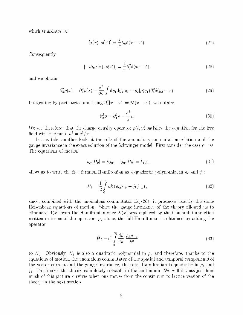
coupling limits of a theory based upon a generalized SLAC-type derivative.

�Work supported by Department of Energy contract DE-AC03-76SF00515.

ye-mail: melnikov@slac.stanford.edu

ze-mail: niv@slac.stanford.edu

1

I. INTRODUCTION

It was argued in an earlier paper [1] that the Contractor Renormalization Group(CORE)

method can be used to map a theory of lattice fermions and gauge �elds into an equivalent

highly frustrated anti-ferromagnet. Although explicit computations were presented only

for the free fermion theory, it was argued that a corresponding mapping must exist for the

interacting theory because the space of retained states used for the free theory coincides with

the set of lowest energy states of the strongly coupled gauge theory. While this argument

is true, it is obviously important to have a better understanding of the details of how the

mapping works. In order to get some experience with this process for a theory which is

well understood we decided to study the lattice Schwinger model (i.e., two-dimensional

QED), since the exact continuum solution of this model exists. Before diving into the

CORE computation, however, we �rst needed to understand the degree to which the lattice

model exhibits the interesting features of the continuum theory. This paper is devoted to

an analytical treatment of the lattice Schwinger model with an eye to clarifying the physics

which underlines the continuum solution and identifying those general features of the model

which should provide an ultimate check of the correctness of any numerical solution.

The continuum Schwinger model [2{7], in addition to being a non-trivial interacting

theory of fermions and gauge �elds, provides a laboratory for studying a wide range of

interesting phenomena. It exhibits: con�nement of the fermionic degrees of freedom and

the concomitant appearance of a massive boson in the exact spectrum; breaking of chiral

symmetry through the axial anomaly; screening of external charges and background electric

�elds; in�nite degeneracy of the vacuum states of the theory (theta parameters); and the

ability to produce arbitrary fermionic polarization charge densities by applying an operator

of the form eiRdx�(x)j0

5(x) to the vacuum state (due to the anomalous commutator of the

electric and axial-charge density operators). It is important to ask which of these features can

be understood in the lattice theory before taking the continuum limit and how complicated

a CORE computation has to be in order to extract this physics. Although the literature

contains discussions of various aspects of the model, such as con�nement and the axial

anomaly [8{11], we are not aware of any systematic discussion of the theory which attempts

to parallel the derivation of the continuum solution within the lattice framework. This is

what we do in this paper.

In order to make the physics as transparent as possible we formulate the Hamiltonian

version of the theory in A0 = 0 gauge and only then rewrite it within the super-selected

sector of gauge-invariant states. We then study the Hamilton equations of motion for the

electric charge density operator, whose form is completely determined by the way in which

local gauge invariance is introduced into the lattice theory. Obviously, the form of the

operator equations of motion depends upon the speci�c lattice fermion derivative and so

we study this problem for a wide class of di�erent derivatives; in particular, generalizations

of the so-called SLAC derivative [13], which explicitly maintain the lattice chiral symmetry

and generalizations of the Wilson derivative [12], which break the chiral symmetry for non-

zero momenta. We �nd that all of these approaches produce a satisfactory treatment of the

continuum theory, however the detailed physical picture of how things work varies greatly.

We show that a key issue for connecting the lattice theory to the continuum theory is

which lattice currents go over to the continuum current operators j0(x) and j50(x). Obviously

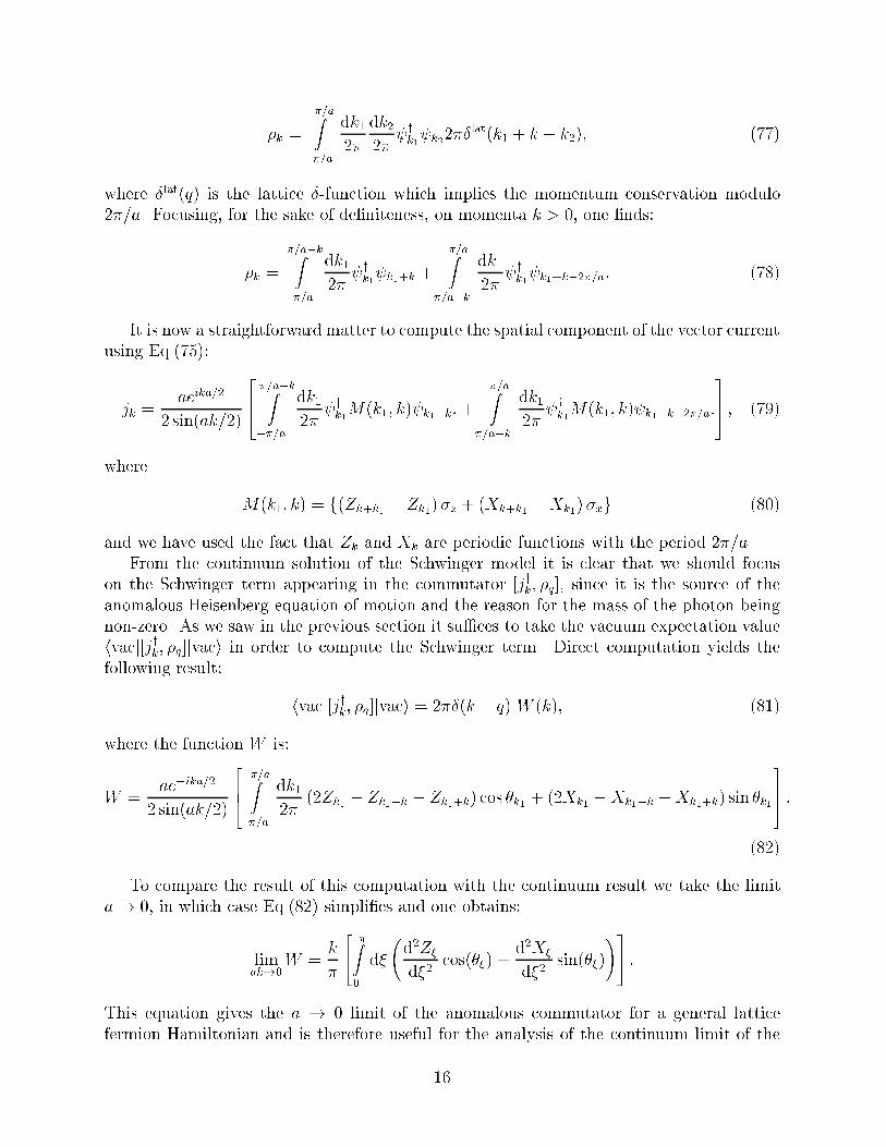
2

the local lattice charge density operator, whose form is �xed by the way in which one

introduces gauge invariance, cannot have this property because the normal ordered version

of this operator satis�es the identity j0(i)3 = j0(i) for all values of the lattice spacing (since

only the charges 0; 1;�1 can exist on a single lattice site). On the other hand, as we will

show, the Fourier transform j0(k) can be treated as a boson operator and the the dynamics

of the theory tells us that the current operators of the continuum theory are obtained by

forming an appropriately regulated version of these lattice operators.

In order to make our discussion essentially self-contained we begin by brie y reviewing

the A0 = 0 gauge treatment of the Hamiltonian version of the continuum Schwinger model.

We discuss: the need for imposing a state condition, such as restricting to gauge-invariant

states; why only the total Q = 0 sector of the theory can exist at �nite energy; and why

di�erent sectors of gauge-invariant states exist and are labelled by a continuous parameter

�1=2 � � � 1=2, which can be identi�ed as a background electric �eld . Finally, we review

the Hamiltonian derivation of the fact that the electric charge density is a free massive Bose

�eld and the role played by the anomalous commutator of the electric and axial charge

density operators in the derivation of this result. After reviewing the continuum theory we

set up and discuss the physics of the lattice version of the Schwinger model in A0(x) = 0

gauge. We then parallel the continuum arguments as closely as possible for a variety of

fermion derivatives. A careful treatment of the Hamilton equations of motion for the Fourier

transform of the charge density operator leads to an understanding of how regulated versions

of these operators go over to the point-split operators of the continuum theory and the sense

in which these regulated operators can be treated as Bose �elds. The di�erence between the

way in which things work for generalized SLAC-type derivatives and Wilson-type derivatives

becomes clear due to this discussion, as does the connection between the strong and weak

coupling theory for generalized SLAC-type derivatives.

II. THE CONTINUUM SCHWINGER MODEL

Hamiltonian formulations of the continuum Schwinger model have been discussed in the

literature [6,7]. Our discussion will parallel these discussions to a degree but will di�er in

important details. Our goal is to allow the reader to understand the important features of

the Schwinger model without unnecessary formalism.

As we have already noted, the Schwinger model is simply QED in 1+ 1 dimensions, and

has a Lagrangian density given by:

L = � (i@� � + eA� �) �1

4F��F

��: (1)

In 1 + 1 dimensions there are only three anti-commuting matrices, 0; 1; 5, and so

they can be realized in terms of the Pauli �-matrices:

0 = �i�x; 1 = �i�y; 5 = 0 1 = �z: (2)

3

In order to enable us to give the most physical treatment of gauge-invariance of the theory

we choose to work in temporal, or A0(x) = 0, gauge. Making this choice the Lagrangian

density becomes:

L = � (i@� � � eA(x) 1) +1

2(@0A(x))

2: (3)

Here, for convenience, we have denoted the spatial component of the vector potential as

A(x) and dropped its subscript. Eq.(3) tells us that the electric �eld,

E(x) = @0A(x); (4)

is the canonical momentum conjugate to A(x) and it has the usual equal-time commutation

relations with A(x):

[E(x); A(x0)] = �i�(x� x0): (5)

Similarly, the fermion operators satisfy the anti-commutation relations

f y�(x); �(x0)g = �(x� x0)���: (6)

It follows immediately that the Hamiltonian in A0 = 0 gauge is

H =

Zdx

"E(x)2

2+ y(x) (i@1 + ieA(x)) �z (x)

#: (7)

There is an essential piece of the physics of working in A0 = 0 gauge which requires

discussion. Since we begin by setting A0 = 0 in the Lagrangian, we cannot vary L with

respect to A0 or @0A0, and so we do not obtain Gauss' law

G(x) =�@xE(x)� e y(x) (x)

�= 0 (8)

as an operator equation of motion. In fact, using the canonical commutation relation, Eq.(5),

we see that

e�iRdy�(y)A(y) G(x) ei

Rdy�(y)A(y) =

�@x(E(x) + �(x))� e y(x) (x)

�= G(x) + @x�(x): (9)

This means that even if we start with a state j�i for which

G(x)j�i = 0; (10)

we can generate states of the form

j��i = eiRd��(�)A(�)j�i (11)

for which

G(x) j��i = @x�(x)j��i: (12)

4

Fortunately, the operators G(x) (which we identify with the generators of time-independent

gauge transformations) commute with one another and with H, and so they can all be

simultaneously diagonalized. Thus we are free to impose Eq.(10) as a state condition because

the Hamiltonian cannot take us out of this sector of the Hilbert space. Actually, we are free

to impose the more general condition of Eq.(12) for any arbitrary function �(x). What

all this means is that the canonical quantization of the Schwinger model in A0 = 0 gauge

produces not one, but rather an in�nite number of theories distinguished from one another

by the fact that they have, in addition to the dynamical fermion �elds, di�erent static

classical background charge distributions �(x)class = @x�(x). This shouldn't be a surprise

because one should be able to formulate QED in the presence of an arbitrary distribution

of static classical background charges. By quantizing in A0 = 0 gauge all we are doing is

obtaining all of these possibilities at the same time.

Since, on physical grounds, we are not interested in formulating the Schwinger model in

the presence of any non-dynamical charge density, it is customary to limit attention to the

so-called gauge-invariant states de�ned by the condition that �(x)class = 0. Note that this

doesn't quite reduce us to a single possibility since all it means is that @x�(x) = 0 or, in other

words, �(x) can be an arbitrary constant. If we make such a transformation we shift the

operators E(x) by a constant, which means that we are free to formulate the theory in the

presence of a constant background �eld �. If we worked in �nite volume this would amount to

allowing for the possiblity that there are non-vanishing classical charges on the boundaries;

i.e. the remaining sectors of the theory di�er by a choice of boundary conditions. One key

question associated with the Schwinger model is whether or not the physics is di�erent for

di�erent values of the background �eld. In particular, does the ground-state energy density,

which is certainly di�erent for the free theory, depend upon the value of � when interacting

fermions are introduced into the game.

A simple argument given by Coleman [5] shows that values of � which di�er by an integer

must be equivalent to one another. Before giving the details of the argument it is important

to note that in one dimension the solution to the equation

@xE(x) =Xj

ej �(x� xj) (13)

for a set of charges ej located at positions xj only has a �nite energy solution when the

total chargeP

j ej = 0. This is so because Eq.(13) tells us that in the regions between the

two charges E(x) is constant and it changes by an amount ej at each point xj. If the sum

of the ej's is not zero then, assuming the �eld vanishes to the left of the �rst charge at x1,

the �eld must continue to in�nity to the right of the last charge. This means that in order

to minimize the �eld energyRE2(x)=2 one or more of the charges must move o� to in�nity

leaving behind a totally neutral system. In particular, if we assume no background �eld

then the energy of a pair of particles with charges �1 separated by a distance s is s=2. In

the presence of a background �eld � > 0 the situation is di�erent. When the �eld is present,

there is a background energy density equal to �2=2. If one now separates a pair of charges

oriented so as to reduce the �eld between the charges to ��1, the total change in the energy

of the system is given by

�E =(�s�2 + s(�� 1)2)

2=s(1� 2�)

2; (14)

5

where the term �s�2 occurs because in the region of length s we have replaced the original

background �eld � by ��1. From Eq.(14) it follows that for � < 1=2 increasing the separation

between the charges costs energy, while for � > 1=2 separating the charges will gain energy

(i.e., by moving the charges o� to in�nity one reduces the background �eld to �0

= �� 1 and

gains an in�nite amount of energy). Clearly with that kind of energy gain nothing can stop

this process from happening and, since the only change in the problem is that now there will

be pairs of charges at �1, it will continue until the background �eld is reduced to the region

�1=2 � � � 1=2. For historical reasons this reduced range of � is usually parametrized by an

angle � = 2�� and is one of the two angles which label the exact solutions to the continuum

Schwinger model [3,5].

If we work in the sector of physical states for which

Qtotj�i = e

1Z�1

d� �(�)j�i = 0; (15)

we can solve for E(x) in terms of �(x)

E = e

xZd� �(�); Qtot = e

1Z�1

d� �(�) = 0: (16)

Substituting this into the Hamiltonian we obtain

H =

Zdx ~ y(x)i@x�z ~ (x)�

e2

4

Zdxdy~�(x)jx� yj~�(y); (17)

where ~ (x) = e�iR x�1

d� A(�) (x). This �eld transformation enables us to eliminate the term

A(x) from the Hamiltonian and simultaneously preserve the canonical commutation relations

of operators (x), y(x). It is important to observe that even if we had not been able to

eliminate E(x) from the Hamiltonian we could have still made this de�nition but it would

not have been particularly useful since in that case E(x) would have non-trivial equal time

commutators with the fermion �elds and we couldn't use the canonical quantization rules

to carry out computations. Note, in what follows we will, by abuse of notation, drop the

tilde and simply write ~ (x) as (x).

The content of the exact solution of this model is that it is the theory of a free boson

of mass m2 = e2=� and, moreover, the charge density operator �(x) can be used as an

interpolating �eld for this particle because it satis�es a free �eld equation with the same

mass. To see how this happens all we need to do is derive the Heisenberg equations of

motion for �(x).

The time derivative of �(x) is

@0�(x) =1

i[�(x); H]: (18)

Since �(x) commutes with itself, we use canonical equal time anti-commutation relations for

the fermionic �elds Eq.(6) and obtain:

@0�(x) = @xj(x); (19)

6

where j(x) = y(x)�z (x). Eq.(19) simply states that divergence of the vector current

vanishes; i.e., the vector current is conserved.

The second derivative of the charge density operator is now given by

@20�(x) =1

i[@xj(x); H]; (20)

which evaluates to

@20�(x) = @2x�(x)�e2

4

Zdy1dy2jy1 � y2j (�(y1)[�i@xj(x); �(y2)] + [�i@xj(x); �(y1)]�(y2)) :

The key point in the solution of the Schwinger model is the commutator of j(x) and

�(x0). It is known that this commutator acquires a Schwinger term which we will compute

by considering Fourier components of the currents:

�(x) =

Zdk

2�e�ikx�k; j(x) =

Zdk

2�e�ikxjk: (21)

By introducing creation and annihilation operators for the upper uk and lower dk com-

ponents of the fermion �elds with standard anticommutation relations:

fuyk; uqg = 2��(k � q); fdyk; dqg = 2��(k � q); (22)

one obtains:

[jk; �q] =

Zdl

2�

�uy

l�k ul+q � uy

l�k�q ul � (u! d)�: (23)

At �rst sight, this is zero, since the integration momenta l can be shifted l! l�q in the �rstterm of the integrand. This, however, is not true. The problem is that the momenta shifts

can be safely done only in the operators that are normal ordered with respect to the vacuum

state, otherwise the di�erence of two in�nite c-numbers appears. Since, in this basis, the

e = 0 Hamiltonian H0 reads:

H0 =

Zdk

2�k�uy

kuk � dy

kdk�; (24)

the vacuum (the lowest energy eigenstate of H0) is obtained by �lling all negative energy

states

jvaci =Yk<0

uy

k

Yk>0

dy

kj0i; (25)

where j0i is the state annihilated by the uk's and dk's. One may see, that for q 6= �k in

Eq.(23), the right hand side annihilates the vacuum and hence momenta shifts are allowed.

For k = �q, however, this is not the case, and that can be easily seen by considering

[jk; ��k]jvaci. One �nally obtains:

[jk; �q] =k

�2��(k + q); (26)

7

which translates to:

[j(x); �(x0)] =i

�@x�(x� x0): (27)

Consequently

[�i@xj(x); �(x0)] =1

�@2x�(x� x0); (28)

and we obtain:

@20�(x) = @2x�(x)�e2

2�

Zdy1dy2jy1 � y2j�(y1)@2x�(y2 � x): (29)

Integrating by parts twice and using @2xjx� x0j = 2�(x� x0), we obtain:

@20� = @2x��e2

��: (30)

We see therefore, that the charge density operator �(t; x) satis�es the equation for the free

�eld with the mass �2 = e2=�.

Let us take another look at the role of the anomalous commutation relation and the

gauge invariance in the exact solution of the Schwinger model. First consider the case e = 0.

The equations of motion

[�k; H0] = kjk; [jk; H0] = k�k; (31)

allow us to write the free fermion Hamiltonian as a quadratic polynomial in �k and jk:

H0 =1

2

1Z0

dk (�k��k + jkj�k) ; (32)

since, combined with the anomalous commutator Eq.(26), it produces exactly the same

Heisenberg equations of motion. Since the gauge invariance of the theory allowed us to

eliminate A(x) from the Hamiltonian once E(x) was replaced by the Coulomb interaction

written in terms of the operators �k alone, the full Hamiltonian is obtained by adding the

operator

HI = e21Z0

dk

2�

�k��k

k2(33)

to H0. Obviously, HI is also a quadratic polynomial in �k and therefore, thanks to the

equations of motion, the anomalous commutator of the spatial and temporal components of

the vector current and the gauge invariance, the total Hamiltonian is quadratic in �k and

jk. This makes the theory completely solvable in the continuum. We will discuss just how

much of this picture survives when one moves from the continuum to lattice version of the

theory in the next section.

8

To complete the usual bosonization of the theory we observe that �k and jk don't satisfy

canonical commutation relations, however a simple rescaling remedies this problem and at

the same time casts the Hamiltonian into a more familiar form. To be precise, since �k has

no k = 0 term1, we can de�ne

�k =

p�

k�k; �k =

p� jk: (34)

Then, using Eq.(26), we see that

[�k; �q] = 2��(k + q); (35)

and the Hamiltonian takes the form

H =

Z1

0

dk

2�

�k��k + (k2 +

e2

�)�k��k

!: (36)

Given the canonical commutation relations for �k and �k and this form of the Hamiltonian,

it is obvious that we are dealing with the theory of a free massive Bose �eld.

Let us now turn to the question of the dependence of the theory on the background

electric �eld, or rather to the more general question of what happens in the Schwinger model

if we introduce static classical charges. The remarkable property of the Schwinger model is

that independent of their magnitude these charges are screened completely. Understanding

how this occurs will fully answer the question of how the theory depends upon a background

electric �eld, since we already noted that having a background �eld of magnitude �1=2 �� � 1=2 corresponds to having classical charges of magnitude �� on the boundaries (or

equivalently at �1 ).

From the solution of the theory in terms of j(x) it is easy to understand the screening

phenomena, since it follows immediately from Eq.(30). Let us consider the Schwinger model

with two external charges of the opposite sign:

�ext(x) = eQext (�(x� x1)� �(x� x2)) : (37)

As we have seen already, Eq.(10) gets modi�ed to include the external charge density. For

this reason the part of the Hamiltonian corresponding to the Coulomb interaction acquires

an additional term and the new equation of motion becomes:

@20� = @2x�� �2 (�(x) + �ext(x)) ; (38)

where �2 = e2=�. This equation implies that there is now a classical, time-independent

component of the charge density operator induced by the external charge which satis�es:

�ind(x) = ��2eQext

Zdk

2�

cos(kjx� x1j)k2 + �2

� (x1 ! x2): (39)

1�0 6= 0 would imply that the system is not neutral and that would violate the state condition

G(x)j�i = 0.

9

Computing the integral, we obtain for the induced charge density:

�ind = �eQext�

2

�e��jx�x1j � e��jx�x2j

�; (40)

which, as advertised, screens the external charge densities. One interesting feature of the

screening is that two external charges get screened independently from each other [7]. Note

also that the screening occurs on the scales �x � 1=�, which for small coupling constant

can be rather large. Nevertheless, if we now move the external charges o� to in�nity, so as

to go over to the sector which in the free theory would have an external background �eld, we

see that this �eld is totally screened in the groundstate of the interacting theory. Moreover,

since all of the screening takes place within a �nite distance of the boundary, there is no

contribution to the groundstate energy density coming from the background �eld.

We should point out that while the previous computation makes it clear that there

shouldn't be a change in the energy density of the groundstate, it is not at all obvious that

there isn't a �nite change in the energy of the state due to the regions surrounding the

screened external charge. In fact, there clearly is such a change when the external charges

are located at a �nite distance from one another; however, the question of what happens as

one moves these charges to plus and minus in�nity is a bit subtle. The crux of the issue

has to do with a de�nition of the limiting process. As will become apparent in a moment

the conventional treatment of the Schwinger model amounts to a prescription in which one

de�nes the Hamiltonian of the system as a limit

H = lim!1

H = lim!1

Zd� H(�) (41)

where is the closed �nite interval = [�!; !]. With this de�nition in mind the usual

prescription is to �rst take the classical background charges to plus and minus in�nity and

then to take the limit !1. Given this prescription it is clear that the total Hamiltonian

de�ned in this way never sees the classical screened charges and therefore there is no change

in the vacuum energy. In order to see that this is the usual prescription which follows from

bosonization of the model let us go back to Eq.(36) and modify it to include the possibility

of having an arbitrary external classical charge density �ext(x). In con�guration space we

obtain:

H =

Zdx

1

2�(x)2 +

1

2(@x�(x))

2 +e2

�(�(x) + �(x))2

!; (42)

where �(x) is the function which satis�es the equation

�ext(x) =1p�@x�(x): (43)

Now, if we set �(x) equal to a constant � we see that all we have to do is de�ne ~�(x) = �(x)+�

and the Hamiltonian becomes identical to the one without a background �eld:

H =

Zdx

1

2~�(x)2 +

1

2(@x~�(x))

2 +e2

�~�(x)2

!: (44)

10

This is the usual way of handling this issue and so we see that this treatment says that

the groundstate energy is independent of the external constant background �eld, which

corresponds to the prescription we gave above.

To complete our discussion of the continuum Schwinger model we present another way

of seeing the screening of the classical background �eld which doesn't require working with

the exact solution to the problem, but only the anomalous commutation relation of �(x)

and j(x). The key to this discussion is the introduction of the conserved gauge-dependent

current

~j(x) = j(x) +e

�A(x): (45)

Obviously, since A(x) doesn't commute with the gauge-generators G(x) de�ned in Eq.(8),

this current mixes states which satisfy di�erent forms of the general state-condition de�ned

in Eq.(11). This means that we should think of ~j(x) as operating in the full Hilbert space of

the theory obtained by canonical quantization in A0 = 0 gauge without imposing any gauge

condition. To show that ~j(x) is conserved we commute it with the Hamiltonian to obtain

@0~j(x) =1

i

h~j;H

i=

1

i[j(x); H] +

e

i�[A(x); H] : (46)

Now, a slight rewrite of the derivation of Eq.(30) gives

1

i[j(x); H] = @0j(x) = @x�(x)�

e2

�@�1x �(x) = @x�(x)�

e

�E(x) (47)

and since by construction @oA(x) = E(x), we obtain

@0~j(x)� @x�(x) = 0; (48)

which means the current is conserved. Integrating this equation over all space we obtain,

under the usual assumptions about surface terms, that�Zdx ~j(x); H

�= 0; (49)

a fact we will use in a moment.

To understand the signi�cance of the fact that ~j(x) is conserved imagine that we start

in a sector of the theory whose lowest energy state satis�es h0jG(x)j0i = 0. Next consider

the transformed state

U(�) j0i = eiRd��(�)(j(�)+ e

�A(�))j0i: (50)

We already saw in Eq.(11) and Eq.(12) that the e�ect of the term proportional to A(�) in

the exponent is to shift the �eld E(x) so that

h0jU y(�)G(x)U(�)j0i = e

�@x�(x): (51)

This equation says that U(�) takes us from a state with no background charge density

to one with background charge density equal to e@x�(x)=�. Similarly, it follows from the

commutations relations of �(x) and j(x) and an integration by parts, that

11

h0jU y(�) �(x)U(�)j0i = � e�@x�(x): (52)

Thus, the total e�ect of applying U(�) to the vacuum of sector of the theory with no classical

charges is to map this state into a sector which has a non-vanishing classical charge density

and at the same time to produce a fermionic charge polarization which cancels it exactly.

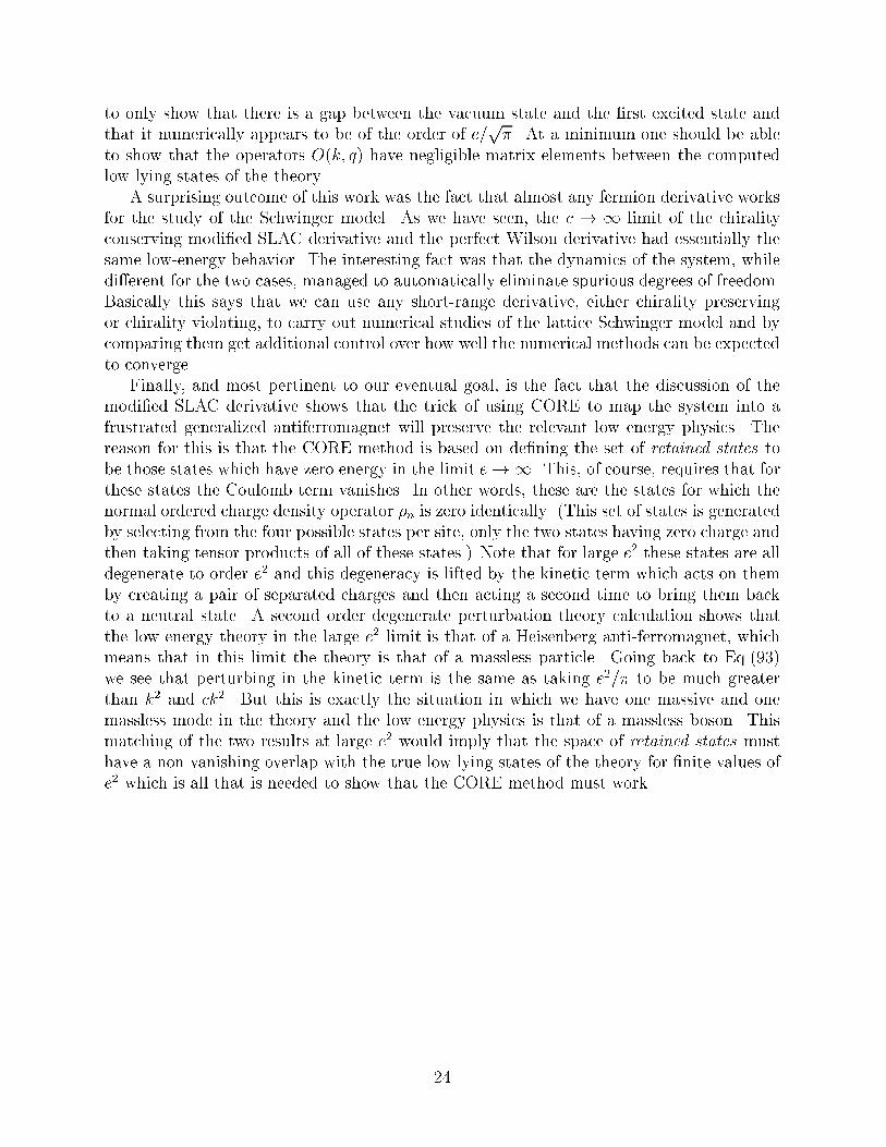
Now imagine that �(x) is chosen as in Fig.1. Since @x�(x) vanishes except in the two narrow

regions around xL and xR we see that the e�ect of this operator is to map the original state

into one which has equal and opposite classical charge densities around xL and xR and

induced cancelling fermionic polarization charge densities. As we move xL and xR to minus

and plus in�nity respectively the function �(x) becomes a constant and in the limit, the fact

that U(�) commutes with H implies that

h0jU yHU j0i = h0jHj0i: (53)

Hence, the energy of the vacuum of the sector with an arbitrary background �eld is the same

as the energy of the vacuum of the sector with no background �eld, which agrees with the

previous argument for the bosonized version of the theory.

III. THE LATTICE SCHWINGER MODEL

Let us now discuss the Hamiltonian version of the Schwinger model on a lattice. In

the Hamiltonian formalism time is continuous and space is taken to be an in�nite lattice

whose points are separated by a distance a. As in the continuum, we work in A0 = 0 gauge.

Furthermore, we introduce fermionic variables yn and n associated with each site on the

spatial lattice and replace the continuous �elds A(x) and E(x) by conjugate variables An

and En associated with the link (n; n + 1) joining the sites n and n + 1. This leads to a

lattice Hamiltonian of the form

H = HE +Hf ; (54)

where

HE =a

2

Xn

E2n; Hf =

Xn;n

0

( yn)�K(n� n

0

)�� e�ie

Pn0

�1

j=nAj ( n0 )

�: (55)

Here the kinetic term K(n�n0)�� is a two-by-two matrix for each value of n�n0 , the fermion

�elds satisfy the anti-commutation relationsn( yn)

�; ( n0 )�o= �n;n0��;� (56)

and the link �elds satisfy the usual harmonic oscillator commutation relations

[An; En0 ] = i�n;n0 : (57)

Note that the fermion �elds are dimensionless and in order to make the connection to

continuum �elds we will have to rescale them by a factor of 1=pa to give them dimensions

12

of mass1=2. In direct analogy to the continuum theory, the eigenvalue of the operator En is

the electric ux carried by the link (n; n + 1). Since, as we have seen, the operator e�ieAn

shifts the ux on the link (n; n + 1) by e it follows that if we de�ne the normal ordered

charge density operator to be

�n =: ( y

n n) :; (58)

then the operators

G(n) = En+1 � En � e�n (59)

commute with the Hamiltonian. Hence, similar to the continuum, we are free to impose the

discrete version of Gauss' law

G(n) j�i = �classn j�i (60)

as a general state condition. Therefore we see that the lattice and continuum versions of the

Schwinger model are essentially the same, in that canonical quantization in A0 = 0 gauge

gives not one version of two-dimensional QED but rather an in�nite number of versions of

the theory corresponding to quantizing in the presence of an arbitrary classical background

charge distribution. Note that the form of Gauss' law expressed in Eq.(60) requires us to use

the local charge density operator �n as the lattice analog of the continuum charge density

operator.

Paralleling the discussion of the continuum theory as closely as possible, we focus at-

tention on the zero charge sector of the space of gauge-invariant states; i.e., the ones that

satisfy the state condition

G(n)j�i = 0: (61)

Once again, in this sector we can explicitly solve for En in terms of �n and eliminate the

factors of eieAn by incorporating them in the de�nition of n. In this way, in the Q = 0

sector of gauge-invariant states, the lattice Hamiltonian can be written as:

H = Hf �e2 a

4

Xn;m

�njn�mj�m: (62)

Because the kinetic term K(n�n0)�� is a function of the di�erence of n and n0

we can write

the Hamiltonian in momentum space as:

H =

�=aZ��=a

dk

2� y

k fZk�z +Xk�xg k +e2a2

4

�=aZ��=a

dk

2�

�k ��k

1� cos ak: (63)

Here we have rewritten the Fourier transform of K(n � n0

)�� in terms of two functions Zk

and Xk, allowing for a very general class of fermion derivatives. Note that in Eq.(63) and all

the equations to follow we have adopted the convention that all momentum space operators

are normalized in a way that the continuum limit is reproduced by taking a ! 0 without

any additional �eld renormalization. For example:

13

f( yk)�; ( q)�g = 2��(k � q)���: (64)

Taking our clue from the discussion of the continuum theory we now turn to the derivation

of the Heisenberg equations of motion for the current �n. The �rst step, namely computing

@0�n =1

i[�n; H] ; (65)

leads us to identify the result of this computation with the divergence of the spatial compo-

nent of the vector current (or, alternatively, the time component of the axial-vector current)

jn. Since the discussion to follow is necessarily a bit detailed it is helpful to summarize what

it will show us in advance. First, we will see that unlike the charge density operator the

current jn is intrinsically point-split as a consequence of the equations of motion. Second, as

in the continuum, the important part of the computation of @0jn, by taking its commutator

with H, involves commuting the jn and �n. This computation will show that one cannot

solve the lattice Schwinger model exactly for any �nite value of the lattice spacing a because

this lattice commutation relation is not the same as its continuum counterpart. Note that

this feature is related to the properties of the free lattice Hamiltonian rather than being a

consequence of the interaction. The same computation will show that the continuum limit

of the naive commutators does not approach the continuum values for the Schwinger model;

from this we will see why, on dynamical grounds, one has to study what amounts to a

point-split version of �n in order to get the correct physics.

For the purpose of illustration, let us consider explicit forms of Xk and Zk corresponding

to a number of popular fermion derivatives. In the case of the naive fermion derivative

Zk = sin(ka)=a; Xk = 0; in the case of the Wilson fermion derivative Zk = sin(ka)=a; Xk =

r=a (1 � cos(ak)); and for the SLAC derivative one has Zk = k; Xk = 0. Given any one

of these derivatives it is easy to �nd the one-particle energy levels of the non-interacting

Hamiltonian Hf by rotating the �elds:

�k = Uk k; (66)

where

Uk = ei �2�y = cos

�

2

!+ i�y sin

�

2

!; (67)

and

cos �k =Zk

Ek

; sin(�k) =Xk

Ek

; Ek =qX2

k + Z2k :

This unitary transformation diagonalizes the Hamiltonian:

Hf =

�=aZ��=a

dk

2�Ek �

y

k�z�k; (68)

and if we introduce creation and annihilation operators for the �-�elds

�k =

ukdk

!; (69)

14

with fuyk; uqg = 2��(k � q) and fdyk; dqg = 2��(k � q), we obtain:

Hf =

�=aZ��=a

dk

2�Ek

�uy

kuk � dy

kdk�: (70)

Finally, the vacuum state of the free theory is obtained by �lling the negative energy sea;

i.e.,

jvaci =Y

��=a<k<�=a

dy

kj0i: (71)

Given these equations it is a straightforward matter to compute the commutator of H

with �n to obtain @0�n:

@0�n =1

i[�n; H]; (72)

which in the continuum theory is equal to @xj(x) (where j(x) is identi�ed as the spatial

component of the vector current, or the time component of the axial-vector current). Com-

puting the commutator of H with �n is straightforward but we must say a few words about

how we identify jn. Basically, in order to maintain the parallel to the continuum discussion

we de�ne the quantity equal to @0�n as the lattice derivative of jn; i.e.,

@0�n =1

a(jn+1 � jn) : (73)

With this identi�cation, the algebra of matrices in two dimensions ensures that the spatial

component of the vector current coincides with the temporal component of the axial current,

and therefore all the currents we are going to work with appear to be de�ned. Clearly,

di�erent lattice fermion derivatives will produce di�erent de�nitions of the spatial component

of the vector current operator, an inescapable consequence of the Heisenberg equations of

motion.

To derive an explicit form for jn, we Fourier transform Eq.(73). De�ning

�k =Xn

�neikan; (74)

we obtain:

@0�k =1

i[�k; H]: (75)

Writing the right hand side of this equation as:

1

a

Xn

(jn+1 � jn) eikan =

�2i sin(ak=2)e�ika=2a

jk; (76)

de�nes the Fourier transform of the spatial component of the vector current. Explicit com-

putation of �k yields:

15

�k =

�=aZ��=a

dk1

2�

dk2

2� y

k1 k22��

lat(k1 + k � k2); (77)

where �lat(q) is the lattice �-function which implies the momentum conservation modulo

2�=a. Focusing, for the sake of de�niteness, on momenta k > 0, one �nds:

�k =

�=a�kZ��=a

dk1

2� y

k1 k1+k +

�=aZ�=a�k

dk1

2� y

k1 k1+k�2�=a: (78)

It is now a straightforward matter to compute the spatial component of the vector current

using Eq.(75):

jk =aeika=2

2 sin(ak=2)

264�=a�kZ��=a

dk1

2� y

k1M(k1; k) k1+k: +

�=aZ�=a�k

dk1

2� y

k1M(k1; k) k1+k�2�=a:

375 ; (79)

where

M(k1; k) = f(Zk+k1 � Zk1)�z + (Xk+k1 �Xk1)�xg (80)

and we have used the fact that Zk and Xk are periodic functions with the period 2�=a.

From the continuum solution of the Schwinger model it is clear that we should focus

on the Schwinger term appearing in the commutator [jy

k; �q], since it is the source of the

anomalous Heisenberg equation of motion and the reason for the mass of the photon being

non-zero. As we saw in the previous section it su�ces to take the vacuum expectation value

hvacj[jyk; �q]jvaci in order to compute the Schwinger term. Direct computation yields the

following result:

hvacj[jyk; �q]jvaci = 2��(k � q) W (k); (81)

where the function W is:

W =ae�ika=2

2 sin(ak=2)

264

�=aZ��=a

dk1

2�(2Zk1 � Zk1�k � Zk1+k) cos �k1 + (2Xk1 �Xk1�k �Xk1+k) sin �k1

375 :

(82)

To compare the result of this computation with the continuum result we take the limit

a! 0, in which case Eq.(82) simpli�es and one obtains:

limak!0

W =k

�

24 �Z0

d�

d2Z�

d�2cos(��) +

d2X�

d�2sin(��)

!35 :

This equation gives the a ! 0 limit of the anomalous commutator for a general lattice

fermion Hamiltonian and is therefore useful for the analysis of the continuum limit of the

16

various choices for the fermion derivative. To get a feeling for how things work let us consider

several speci�c examples.

Let us begin with the case of the naive lattice fermion derivative, where Z� = sin �,

X� = 0, E� = j sin �j. In this case we obtain:

limak!0

W = �k�

�Z0

d� sin � = �2k

�: (83)

This shows that the anomalous commutator is two times larger than the continuum result,

which implies that in the a ! 0 limit the mass of the photon is two times larger than in

the continuum theory. In principle, this result should have been expected since the lattice

theory with the naive fermion derivative has an exact SU(2) symmetry for all values of a

and as a consequence of this symmetry the fermion spectrum is doubled as is evident from

the form of Ek. Thus, it follows that the continuum limit of the naive theory is not the

original Schwinger model, but rather an SU(2)-Schwinger model which is known to have a

photon mass which is 2e2=�.

In case of Wilson fermions we have Z� = sin �, X� = r(1� cos �) and E� =qZ2� +X2

� .

By explicit calculation one �nds:

limak!0

W = �2k

�; (84)

Once again the result is two times larger than the continuum one2, but in this case the low

energy spectrum is clearly undoubled and the reason for the discrepancy between the lattice

and continuum results must be di�erent.

In order to clarify the underlying physics, it is instructive to consider somewhat un-

conventional fermion derivatives. Let us begin by considering a modi�ed SLAC fermion

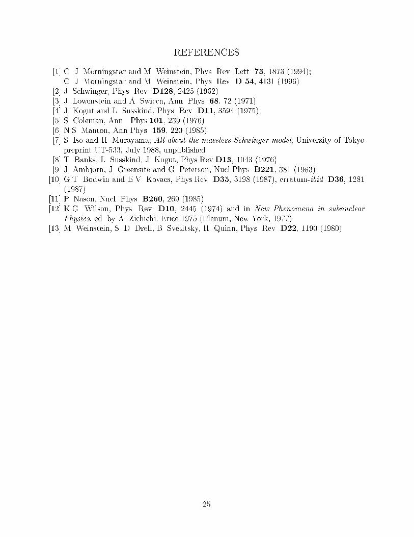
derivative [11]. Consider the free fermion Hamiltonian de�ned by (k > 0, Z�k = �Zk):

Zk = k�

���

a� k

�+

�

�� 1

��

a� k

��

�k � �

�

a

�; Xk = 0; (85)

and Ek is equal to jZkj. A plot of Ek is shown in Fig.2. Computing the second derivative of

Zk one obtains:

�d2Z�

d�2= �

���

a� �

�+

�

1� ��

�� � �

�

a

�; (86)

2The fact that the anomalous commutator for Wilson fermions is r-independent in the a ! 0

limit is a bit of a miracle and we do not quite understand the reason for that. Note however, that

a similar situation has been observed in earlier calculations of the chiral anomaly in the lattice

Schwinger model with Wilson fermions [9]. It is generally accepted that the continuum limit of

the Schwinger model with Wilson fermions gives correct anomaly and correctly reproduces all

other continuum results. However, there is no direct contradiction with our statement since, as we

explained and as our result seem to illustrate, di�erent currents lead to di�erent results.

17

and the anomalous commutator becomes:

limak!0

W =�k�

1 +

�

1� �

!: (87)

To understand the information encoded in this form of the anomalous commutator let us

consider what happens in the continuum limit. It is clear from the plot of Ek for this modi�ed

SLAC derivative that two species of fermions survive in the limit a! 0. Note however that

dEk=dk is quite di�erent for the two linear regions of the spectrum, which means that the two

species propagate with very di�erent speeds. The anomalous commutator is really the sum

of two contributions: one coming from 0 < k < ��=a and the other from ��=a < k < �=a

and these contributions can be easily identi�ed with the di�erent fermions. Since both

fermions are charged, they both contribute to the anomalous commutator and to the mass

gap.

Given the simple nature of this fermion derivative it is clear how to separate the contri-

butions of the two fermion species to the total current. The easiest way to do this is to put

a sharp momentum cut-o� somewhere below and above the turning point ��=a. With this

prescription we write the charge density operator as a sum of three contributions:

�k = �(1)

k + �(2)

k + �(3)

k ; (88)

where

�(1)

k =

�1�=aZ��1�=a

dk1

2� y

k1 k1+k; �

(3)

k =

Zjk1j>�2�=a

dk1

2� y

k1 k1+k +

�=aZ�=a�k

dk1

2� y

k1 k1+k�2�=a; (89)

and �1 < � < �2. The �(2)

k provides for the remaining contribution to the charge density

and it is only sensitive to fermions with momenta �1�=a < jkj < �2�=a. Now, following our

previous argument, we de�ne the corresponding spatial components of the vector current by

explicitly commuting the above charge densities with the Hamiltonian.

A straightforward computation shows that in the limit of vanishingly small lattice spacing

the anomalous commutators of the above currents are given by:

[�j(1)

k

�y; �(1)q ] = �k

�2��(k � q);

[�j(2)

k

�y; �(2)q ] = 0;

[�j(3)

k

�y; �(3)q ] = �ck

�2��(k � q); (90)

where we introduced c = �=(1 � �), which is the velocity of the fermions in the region

k � �. Note that in all of these formulas there are also non-vanishing normal-ordered

operators coming from large momentum excitations which we have not displayed. These

operators annihilate the vacuum and one can argue that they are unimportant for small k

physics. This �nal point, which is intimately related to the sense in which jk can be treated

as a boson operator, merits elaboration and we will return to it immediately after completing

our discussion of the equations of motion.

18

Proceeding with our computation of the equations of motion for �(1)

k and �(3)

k we obtain:

�@20�(1)

k = k2�(1)

k +e2

��totk ;

�@20�(3)

k = c2k2�(3)

k + ce2

��totk ; (91)

where the total charge density operator appears on the right hand side of these equations and

so �(2)

k is still included. Consistent with the point made above and subject to the discussion

to follow we will set it to zero, since for small energies fermions with such high momenta are

not excited.

From the equations for the commutators we see that the �eld �(3)

k is not canonically

normalized and so we introduce the new �eld ~�3k = 1=pc�

(3)

k and its commutation relation

with the corresponding current becomes canonical. The equations of motion become:

�@20�(1)

k = k2�(1)

k +e2

�

��(1)

k +pc~�

(3)

k

�;

�@20 ~�(3)

k = c2k2~�(3)

k +e2

�

�pc�

(1)

k + c~�(3)

k

�: (92)

The energies of elementary excitations can be determined from the eigenvalues of the matrix

M =

k2 + e2=�

pc e2=�p

c e2=� c2k2 + c e2=�

!: (93)

The matrix is easily analyzed in the limit of large c which corresponds to the large slope of

the fermion derivative in the region k � �. Note that the original SLAC fermion derivative

corresponds to c!1 limit.

It is then easy to see that there are two di�erent limits in this equation. For small

momenta ck2 � e2=�, there are two eigenvalues:

E1 =pck; E2 =

p1 + c

e

�:

Hence there is a zero mass eigenstate which is the Goldstone boson of the theory. The other

excitation is the massive one. If we consider the limit c!1, the region of momenta sensitive

to the Goldstone mode shrinks to zero (see Fig.3) and the mass of the other excitation goes

to in�nity.

For larger momenta, ck2 � e2=�, the mixing of two states becomes small, they propagate

independently and their energies are given by:

E1 =

sk2 +

e2

�; E2 =

sc2k2 + c

e2

�: (94)

In this momentum region the energy of the lower excitation approaches the result of the con-

tinuum theory of a bosonic �eld with the mass e2=�, the other excitation becomes in�nitely

heavy and decouples explicitly (see Ref. [11]). Hence, as we approach the limit c ! 1(which is equivalent to the orginal form of the SLAC derivative), the continuum limit of the

19

theory has a massive boson of mass m2 = e2=� and an isolated state at k = 0 which can be

identi�ed with a seized Goldstone mode [4].

Since the main purpose of this paper is to provide an analytic framework for CORE

computations to follow we should point out that the fact that there is a Goldstone mode

when e2=� � ck2 is quite signi�cant since it relates to the whole question of how the strong-

coupling limit of the model connects to the weak coupling theory and whether one can get

the correct physics by projecting onto the sector spanned by the e ! 1 eigenstates. We

will have more to say about this point in the conclusions, but �rst we should complete our

discussion of terms we ignored in the commutator of [jk; �q].

While this preceding argument leading to Eq.(92) makes the lattice discussion look re-

markably like the continuum Schwinger model, we are not really �nished. The issue which

still needs discussion relates to the interpretation of �k and jk as boson �elds. This is more

than an academic issue. Although, as we have shown, the vacuum expectation value of

the commutator of jk and �q gives the required Schwinger term, computation of the full

commutator contains an extra piece which, if it has non-vanishing matrix elements between

states whose energy remains �nite in the a ! 0 limit, ruins the interpretation of jk and �qas boson �elds. This is the issue which we will now address.

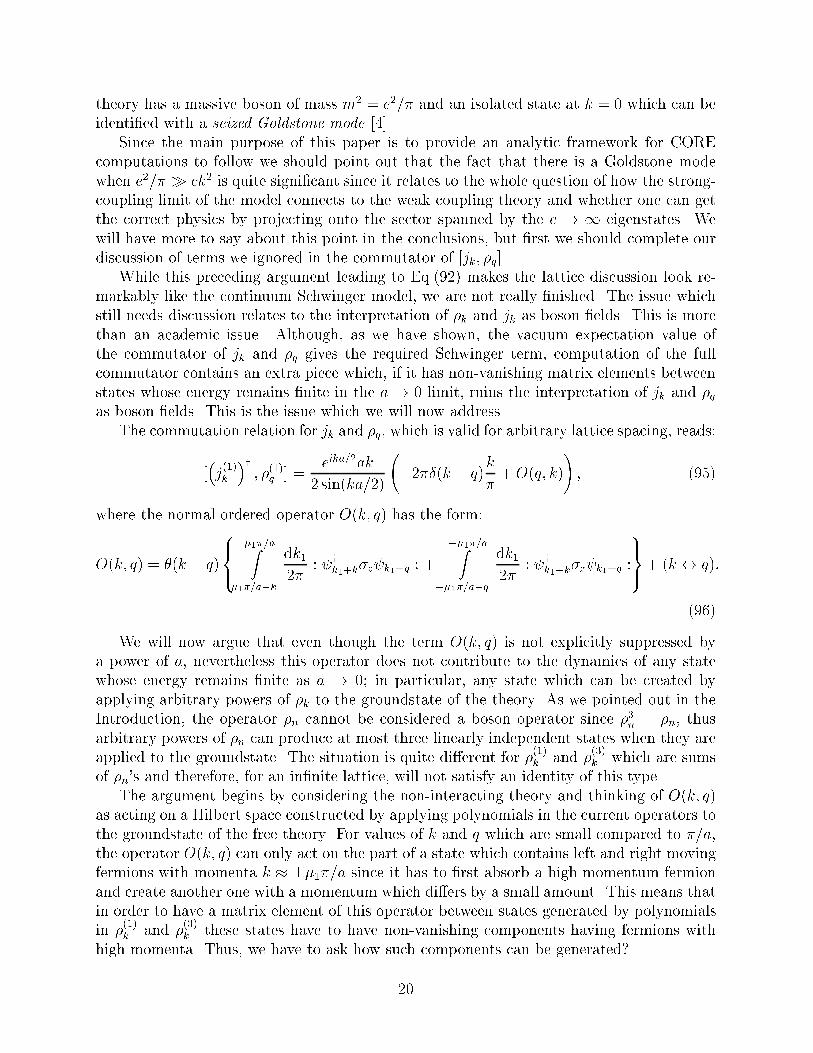
The commutation relation for jk and �q, which is valid for arbitrary lattice spacing, reads:

[�j(1)

k

�y; �(1)q ] =

eika=2ak

2 sin(ka=2)

�2��(k � q)

k

�+O(q; k)

!; (95)

where the normal ordered operator O(k; q) has the form:

O(k; q) = �(k � q)

8><>:

�1�=aZ�1�=a�k

dk1

2�:

y

k1+k�z k1+q : +

��1�=aZ��1�=a�q

dk1

2�:

y

k1+k�z k1+q :

9>=>;+ (k $ q):

(96)

We will now argue that even though the term O(k; q) is not explicitly suppressed by

a power of a, nevertheless this operator does not contribute to the dynamics of any state

whose energy remains �nite as a ! 0; in particular, any state which can be created by

applying arbitrary powers of �k to the groundstate of the theory. As we pointed out in the

Introduction, the operator �n cannot be considered a boson operator since �3n = �n, thus

arbitrary powers of �n can produce at most three linearly independent states when they are

applied to the groundstate. The situation is quite di�erent for �(1)

k and �(3)

k which are sums

of �n's and therefore, for an in�nite lattice, will not satisfy an identity of this type.

The argument begins by considering the non-interacting theory and thinking of O(k; q)

as acting on a Hilbert space constructed by applying polynomials in the current operators to

the groundstate of the free theory. For values of k and q which are small compared to �=a,

the operator O(k; q) can only act on the part of a state which contains left and right moving

fermions with momenta k � ��1�=a since it has to �rst absorb a high momentum fermion

and create another one with a momentum which di�ers by a small amount. This means that

in order to have a matrix element of this operator between states generated by polynomials

in �(1)

k and �(3)

k these states have to have non-vanishing components having fermions with

high momenta. Thus, we have to ask how such components can be generated?

20

Both �(1)

k and �(3)

k are bilinears in fermion creation and annihilation operators and, being

normal ordered, can only absorb a fermion at one momentum and create a replacement at

another momentum. Generically these operators are of the general form:

�(i)k =

Zdk1

2�

�uy

k1uk1+k + d

y

k1dk1+k

�(97)

and since for the modi�ed SLAC derivative Xk = 0, the vacuum, as in the continuum, is

given by Eq.(25). If we now, for the sake of de�niteness, consider

�(1)

k>0jvaci = �(1)

k

Yk<0

uy

k

Yk>0

dy

kj0i (98)

we see that almost all terms in �(i)k annihilate the vacuum state. The only terms which act

non-trivially are ones were either uk1+k or dk1+k can absorb a particle and then either uy

k1or

dy

k1can create a particle. Clearly, for small k > 0 only the dk1 terms can act, since if k1 < 0

and k1+k > 0 then dk1+k can absorb a d from the vacuum state and dy

k1can create a d. The

uk terms cannot act non-trivially because in order for uk1+k to absorb a particle, k1 + k has

to be less than zero, in which case k1 < 0 and therefore uy

k1annihilates the resulting state. If,

however, k < 0 then it is the uy

k1uk1+k term which acts non-trivially and the corresponding

d term annihilates the state. In either event the important point is that the �(i)k only creates

and absorbs particles from the vacuum which are within a distance jkj of the top of the

negative energy sea (i.e., the fermi-surface) thus creating a particle anti-particle pair.

The next step is to see what happens if we apply �(i)k to the state we just generated.

What we get is

�(i)k

2

jvaci = 1

(2�)2

Zdk1 dk2

�uy

k2uk2+k + d

y

k2dk2+k

� �uy

k1uk1+k + d

y

k1dk1+k

�jvaci: (99)

It should be clear that for almost all k1 and k2 in the allowed region �(i)k

2

creates two low

momentum particle anti-particle pairs and in fact for given allowed k1 and k2 there are 2!

ways of getting the same two-pair state; however, for a given k1 there is exactly one value of

k2 for which one can create a higher energy one-pair state by absorbing one of the particles in

the pair created by the �rst application of �(i)k and promoting it to higher momentum. From

this it follows that the factor needed to normalize this state is greater than 1=p2!. Similarly,

if one hits this state with another power of �(i)k almost all of the terms would create three

low energy particle anti-particle pairs and each of these three pair states would be created

3! times. As in the previous case however there would be a single term which could promote

the previous single higher energy one-pair state to yet higher energy. Note, however, that

since the normalization of this state would have to be larger than 1=p3! (which we are

beginning to recognize as the normalization factor which goes with a three boson state)

the coe�cient of this higher energy single-pair state appearing in the normalized version

of the state created by �(i)3

k is getting smaller each time. If one now imagines carrying

out this process p-times the argument generalizes in the obvious way. The state obtained

by applying p powers of �(i)k to jvaci is going to be mostly made of p di�erent low-energy

particle anti-particle states, each of which will be arrived at in p! ways. Furthermore, there

21

will be a single particle anti-particle pair state with individual momenta p times larger than

k. Since now the normalization factor of this state is bigger than p!, the coe�cient of this

single higher energy pair state is getting very small relative to the part of the wavefunction

made of p low energy pair states. A more careful discussion of this point would also take

into account the fact that the same procedure will generate two-pair, three-pair, etc., parts

of the wavefunction. However, the point is that if we keep k � �, where � is a maximal

energy we wish to consider and �a! 0 in the continuum limit, then in order to achieve the

fermionic level with momenta �1�=a, one should create a state jNk jvaci with

N � �1�

ak� �1�

a�!1: (100)

The energy of this bosonic state is � Etyp � �1�=a ! 1; and it is easy to see that the

probability of �nding a single high momentum pair state equals to 1=N !! 0. The factors of

p! which appear in the normalization of the jpjvaci states thus produce the explanation of

both why we can think of �(i)k as a boson operator and why O(k; q) has no signi�cant matrix

elements between normalized states generated by applying arbitrary powers of �(i)k to jvaci.

The main point of the above discussion is that as we approach the continuum limit the

essential physics of the model is taking place near the top of the negative energy sea and so

it is useful to limit our attention to modi�ed operators �(i)k that only have support in these

regions. For the model based upon a modi�ed SLAC derivative we saw that, since the low

energy spectrum of the theory was explicitly doubled, the non-split fermion current really

was made up of two parts: the �rst, coming from states near k � 0 and the other from k � �.

Leaving aside the complications related to the existence of the Goldstone mode, we see that

the dynamics of the theory tells us that the current constructed out of the fermionic �elds

with small momenta is essentially the current with the correct continuum limit. The large

momentum part of the current decouples from the continuum limit after the limit c!1 is

taken. From this point of view, we see that the dynamics of the lattice model tells us that in

order to take the continuum limit of the theory we have to restrict attention to only a part

of the unregulated lattice current. This is essentially equivalent to adopting a point-splitting

procedure for de�ning the current in the continuum theory.

Though these peculiarities have been made obvious because of the explicit doubling,

our calculation of the anomalous commutation relation shows that for the non-point-split

currents the large momentum modes do not decouple automatically, even without fermion

doubling. To have explicit decoupling one has to construct the currents by explicitly cutting

o� the region of large momentum. If in the small momentum region the fermion derivative is

su�ciently continuum-like (i.e., linear) then we are assured that: the current constructed in

this way will have correct anomalous commutation relations modulo corrections suppressed

by inverse cut-o�; the equations of motion for this current will be free equations of motion

with an additional source term given by high momentum fermionic modes; if the cut-o� is

su�ciently large in physical energy units (as opposed to lattice units), such a current operator

will correspond to a continuum bosonic degree of freedom for all low-energy purposes.

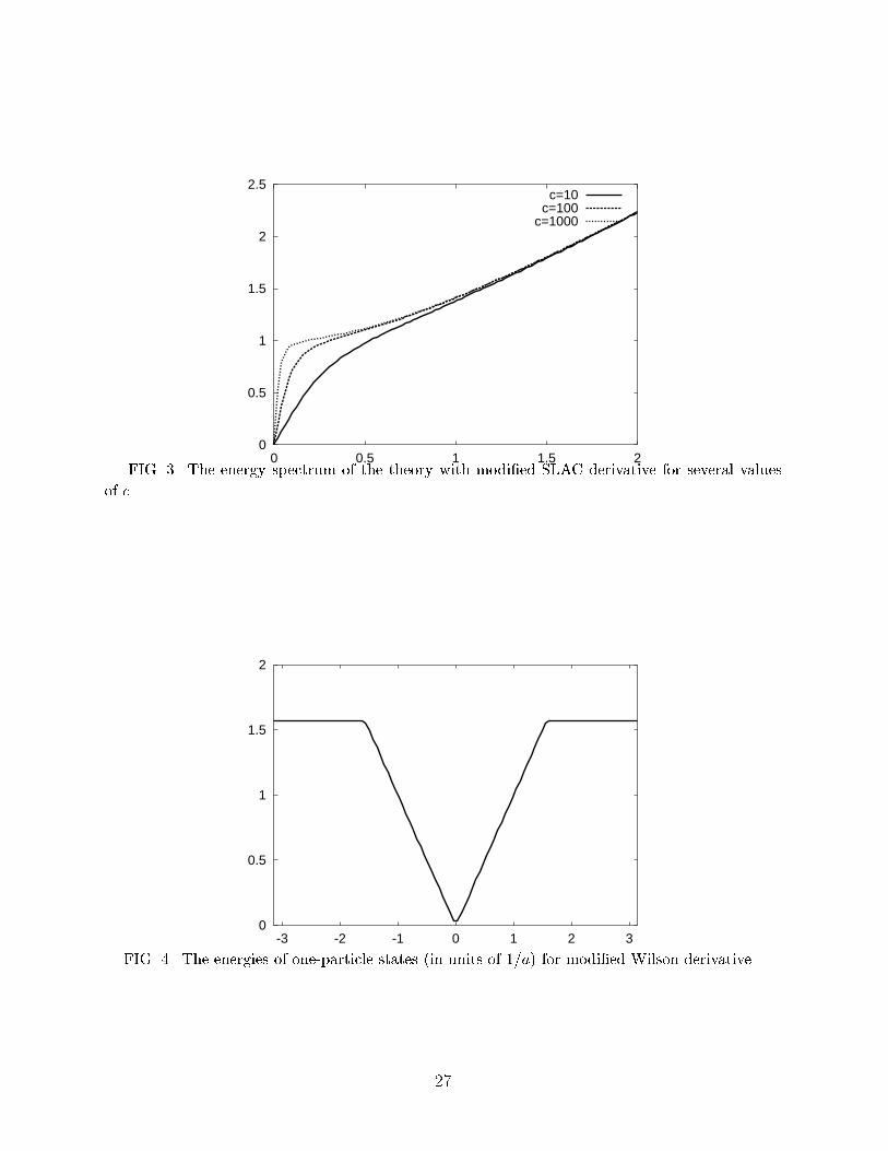
To conclude this section let us consider a simple example of what we will refer to as a

perfect Wilson model for the fermion derivative. It is de�ned by

Zk = k�

��

2a� k

�+

�

2asin (� � ka) �

�k � �

2a

�; Xk =

�

2acos (� � ka) �

�k � �

2a

�;

22

where we have de�ned Zk and Xk for k > 0, and assumed that Z�k = Zk and X�k = Xk.

The one-particle energy spectrum is shown in Fig.4.

One may easily check (using our general result for the anomalous commutator) that for

this model, in the limit a! 0, the commutator for the non-split currents [jk; �q] di�ers from

the continuum limit, even though in this case there is no doubling and the theory remains

continuum-like up to momenta k � �=(2a). Note, however, that if we construct a low energy

current by restricting to the linear region of the derivative function, as in the case of the

modi�ed SLAC derivative, we can guarantee that the high momenta modes do not have an

in uence on the dynamics of the low energy current and we can verify that this low-energy

current and its time derivative satisfy the desired anomalous commutation relations. Once

we establish this fact we can proceed to derive the Heisenberg equations of motion for this

low-energy (or regulated) version of the current and make the connection to the continuum

theory. Conceptually, our example of the perfect Wilson fermion derivative is very close to

Wilson's original proposal. All we have done is to enlarge the region of momentum space

in which the lattice derivative looks identical to the continuum derivative so as to make it

easier to see why this type of fermion derivative works once the proper current operators

have been identi�ed.

IV. CONCLUSIONS

As we have said in the Introduction our aim is to use the lattice Schwinger model to

test the idea that one can use CORE methods to map gauge theories into highly frustrated

spin antiferromagnerst and then use the same methods to study these spin systems. The

Schwinger model is a very good place to test this notion since the continuum model exhibits

a rich spectrum of physical phenomena, anomalous commutators, background electric �elds,

charge screening, etc., and so it is important that any numerical treatment of this model

be able to see these e�ects. We had several major goals in this paper: �rst, to get some

analytic control over the physics of the lattice Schwinger model in order to understand

which features of the continuum theory we might expect to emerge easily from a numerical

computation and which might be di�cult to obtain; second, to gain a feeling for how much

of this physics we might hope to see if we �rst use CORE to map the lattice Schwinger

model into a highly-frustrated generalized antiferromagnet and then to analyze the physics

of that spin system before carrying out detailed numerical computations; third, to get a

better understanding of how the low-energy physics of the lattice system depends upon the

choice of fermion derivative and why, on dynamical grounds, the lattice currents of interest

are those which correspond to continuum point-split currents.

To accomplish our goals we studied Hamiltonian formulations of both the continuum

and lattice Schwinger model and then, by paralleling the solution of the continuum version

of the theory in the lattice framework, identi�ed those features of the lattice theory which

di�er from the continuum theory and identi�ed the operators of the lattice theory which go

over smoothly to their continuum counterparts. It became apparent from the treatment of

the equations of motion for the various forms of the charge density in the lattice theory that

getting the right behavior involves showing that one is close enough to the continuum limit

so that the appropriately de�ned currents act as bosons; in other words, it is not su�cient

23

to only show that there is a gap between the vacuum state and the �rst excited state and

that it numerically appears to be of the order of e=p�. At a minimum one should be able

to show that the operators O(k; q) have negligible matrix elements between the computed

low-lying states of the theory.

A surprising outcome of this work was the fact that almost any fermion derivative works

for the study of the Schwinger model. As we have seen, the c ! 1 limit of the chirality

conserving modi�ed SLAC derivative and the perfect Wilson derivative had essentially the

same low-energy behavior. The interesting fact was that the dynamics of the system, while

di�erent for the two cases, managed to automatically eliminate spurious degrees of freedom.

Basically this says that we can use any short-range derivative, either chirality preserving

or chirality violating, to carry out numerical studies of the lattice Schwinger model and by

comparing them get additional control over how well the numerical methods can be expected

to converge.

Finally, and most pertinent to our eventual goal, is the fact that the discussion of the

modi�ed SLAC derivative shows that the trick of using CORE to map the system into a

frustrated generalized antiferromagnet will preserve the relevant low energy physics. The

reason for this is that the CORE method is based on de�ning the set of retained states to

be those states which have zero energy in the limit e!1. This, of course, requires that for

these states the Coulomb term vanishes. In other words, these are the states for which the

normal ordered charge density operator �n is zero identically. (This set of states is generated

by selecting from the four possible states per site, only the two states having zero charge and

then taking tensor products of all of these states.) Note that for large e2 these states are all

degenerate to order e2 and this degeneracy is lifted by the kinetic term which acts on them

by creating a pair of separated charges and then acting a second time to bring them back

to a neutral state. A second order degenerate perturbation theory calculation shows that

the low energy theory in the large e2 limit is that of a Heisenberg anti-ferromagnet, which

means that in this limit the theory is that of a massless particle. Going back to Eq.(93)

we see that perturbing in the kinetic term is the same as taking e2=� to be much greater

than k2 and ck2. But this is exactly the situation in which we have one massive and one

massless mode in the theory and the low energy physics is that of a massless boson. This

matching of the two results at large e2 would imply that the space of retained states must

have a non-vanishing overlap with the true low lying states of the theory for �nite values of

e2 which is all that is needed to show that the CORE method must work.

24

REFERENCES

[1] C. J. Morningstar and M. Weinstein, Phys. Rev. Lett. 73, 1873 (1994);

C. J. Morningstar and M. Weinstein, Phys. Rev. D 54, 4131 (1996).

[2] J. Schwinger, Phys. Rev. D128, 2425 (1962).

[3] J. Lowenstein and A. Swieca, Ann. Phys. 68, 72 (1971).

[4] J. Kogut and L. Susskind, Phys. Rev. D11, 3594 (1975).

[5] S. Coleman, Ann. Phys.101, 239 (1976).

[6] N.S. Manton, Ann Phys. 159, 220 (1985).

[7] S. Iso and H. Murayama, All about the massless Schwinger model, University of Tokyo

preprint UT-533, July 1988, unpublished.

[8] T. Banks, L. Susskind, J. Kogut, Phys.Rev.D13, 1043 (1976).

[9] J. Ambjorn, J. Greensite and G. Peterson, Nucl.Phys. B221, 381 (1983).

[10] G.T. Bodwin and E.V. Kovacs, Phys.Rev. D35, 3198 (1987), erratum-ibid. D36, 1281

(1987).

[11] P. Nason, Nucl. Phys. B260, 269 (1985).

[12] K.G. Wilson, Phys. Rev. D10, 2445 (1974) and in New Phenomena in subnuclear

Physics, ed. by A. Zichichi, Erice 1975 (Plenum, New York, 1977).

[13] M. Weinstein, S. D. Drell, B. Svetitsky, H. Quinn, Phys. Rev. D22, 1190 (1980).

25

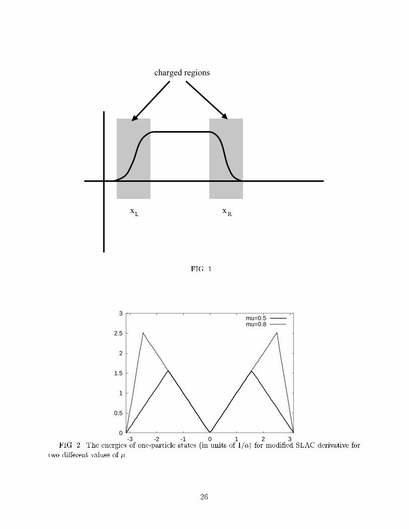
FIG. 1.

0

0.5

1

1.5

2

2.5

3

-3 -2 -1 0 1 2 3

mu=0.5mu=0.8

FIG. 2. The energies of one-particle states (in units of 1=a) for modi�ed SLAC derivative for

two di�erent values of �.

26

0

0.5

1

1.5

2

2.5

0 0.5 1 1.5 2

c=10c=100

c=1000

FIG. 3. The energy spectrum of the theory with modi�ed SLAC derivative for several values

of c.

0

0.5

1

1.5

2

-3 -2 -1 0 1 2 3

FIG. 4. The energies of one-particle states (in units of 1=a) for modi�ed Wilson derivative.

27