SLAG’ - WE3 - 3322

April 1084

w

The t-EXPANSION:

A NON-PERTURBATIVE ANALYTIC TOOL FOR HAMILTONIAN SYSTEMS’

D. HORNS AND M. WEINSTEIN

Stanford Linear Accelerator Center

Stanford University, Stanford, California 04305

Submitted to Physical Review D

* Work supported by the Department of Energy, contract DE - AC03 - 76SFOO515

t On leave from Tel-Aviv University, Israel

ABSTRACT

A systematic non-perturbative scheme is developed to calculate the ground-

state expectation values of arbitrary operators for any Hamiltonian system.

Quantities computed in this way converge rapidly to their true expectation val-

ues. The method is based upon the use of the operator eatH to contract any

trial-state onto the true groundstate of the Hamiltonian H. We express all ex-

pectation values in the contracted state as a power series in t, and reconstruct

the t -+ 00 behavior by means of Pad6 approximants. The problem associated

with factors of spatial volume is taken care of by developing a connected graph

expansion for matrix elements of arbitrary operators taken between arbitrary

states. We investigate Pad& methods for the t-series and discuss the merits of

various procedures. & examples of the power of this technique we present results

obtained for the Heisenberg and Ising models in 1+1 dimensions starting from

_ simple mean-field wavefunctions. The improvement upon mean-field results is re-

markable for the amount of effort required. The connection between our method

and conventional perturbation theory is established; and a generalization of the

technique which allows us to exploit off-diagonal matrix elements is introduced.

This bi-state procedure is used to develop a t-expansion for the ground-state

energy of the Ising model which is, term by term, self-dual.

2

1. INTRODUCTION

It has become clear that analyzing confinement and computing the properties

of hadrons requires the development of non-perturbative methods for dealing

with quantum field theories. Conventional renormalization techniques require

a perturbative framework and so, in order to remove all divergences from the

theory, Wilson I11 introduced a lattice formulation of Euclidean gauge-theories

which was transcribed into Hamiltonian langauge by Kogut and Susskind If one

adopts this formalism the problem becomes one of being able to analyze this sort

of theory for all values of the coupling constant. It quickly became clear that

strong coupling perturbation theory could not be relied upon to study the physics

of the weak coupling limit, i.e. the limit of interest for the continuum theory, and

other techniques would be necessary. Up to now much effort has been invested in

Monte Carlo calculations in an attempt to systematically compute the quantities

. of physical interest. The drawback of the Monte Carlo technique is the amount

of computer time required to study even small lattices; this, of course, makes it

hard to trust these results as guides to the physics of the continuum. Another

drawback of the Monte Carlo technique is that it is entirely numerical and one has

no way of getting a feeling for what is essential and what is superfluous. In order

to obtain information of this nature there would seem to be no substitute for

non-perturbative analytic techniques which can be used to systematically study

Hamiltonian systems in general. In this paper we present a new non-perturbative

scheme which can be applied to a wide class of Hamiltonian lattice theories. While this should be of general interest to people working on many-body and

condensed matter problems, we are particularly attracted to the method because

it holds great promise of working well for lattice gauge-theories. For pedagogical

reasons this paper will focus on some simple Hamiltonian lattice systems in order to present the basic ideas and show how well the approximation scheme converges.

&The application of these techniques to lattice gauge theories will be presented

elsewhere.

3

In looking for a candidate for a non-perturbative computational scheme appli-

cable to a wide variety of problems, one is tempted to turn to variational methods.

There are many variational techniques which allow for non-perturbative calcula-

tion of the ground-state, and low-lying excited states, of a Hamiltonian system.

The principal virtue of these methods is they allow the computation of effects,

such as the existence of phase transitions, which cannot be treated within the

framework of ordinary perturbation theory. Their principal drawback is that

there is no simple scheme for systematically improving upon the initial result.

In the section which follows we will show how to rectify this situation and de-

velop a non-perturbative expansion, henceforth referred to as the t-expansion,

which allows one to systematically improve upon the results of any variational,

or perturbative, calculation. The application of this method to specific examples

shows that successive approximations to quantities of physical interest converge

rapidly to their true ground-state expectation values.

We begin by presenting the simple idea behind this scheme and establish the

rules for calculating in a general theory. Next, we present the results of applying

this technique to some sample problems. After the reader has gotten a feeling

for the way in which the technique works, we establish the connection of this

method to the usual perturbation expansion, and present a generalization of the

basic scheme which may play an important role in the analysis of lattice gauge

theories.

4

2. FUNDAMENTALS

2.1 THE BASIC IDEA

Non-perturbative techniques such as Hartree, Hartree-Fock, mean-field and

real-space renormalization group approximations, are variational calculations for

the ground-state of a Hamiltonian system. In each case one picks a trial state,

I&) , which depends upon a set of variational parameters, {o} = oi, . . . , cr,,,

and determines the best values for these parameters by minimizing

EO(~l,...,%) = (tDol H No) (toolSo) - (2.1)

Assuming that we have chosen such a variational wavefunction we note that the

normalized state

is, for any finite value of t, a better approximation to the true vacuum. To prove

this expand [$J ) t in eigenstates of H, and observe that

e-tH/2 It+!Jt) = C cn e-c~t/21n)e n

(2.3)

It follows from (2.3) that the coefficient of the true vacuum state which appears

in the expansion of I$t) is larger than in I$Jo) . As long as the initial state I$J~)

has an overlap with the true ground-state quantities like

w = Wtl 0 19th (24 and in particular

E(t) = (St1 H ISA (2.5)

-are guaranteed to converge to their true ground-state expectation values in the

limit t --) 00. This contraction of the wavefunction onto the lowest eigenstate

5

of the Hamiltonian rapidly eliminates states which have energies far larger than

the lowest state and if accurately computed, provides an upper bound upon the

ground-state energy for any finite value of t.

2.2 CLUSTEREXPANSION

Focusing on the problem of computing the ground-state energy for a system

defined by a Hamiltonian, H, we see that evaluation of (2.2) and (2.5) requires

the computation of ratios like

E(t) = k-d He-‘H ‘tlto) Wol ctH MO) * P-6)

In general, we cannot exponentiate the Hamiltonian of a quantum system, so some

way of approximating the ratio must be developed. Our approach is to expand

. (2.6) to a fixed order in the variable t and then use PadC approximants to recon-

struct the function. This method is appealing since computing ($01 OH” I&), for

I$+)) belonging to th e class of variational wavefunctions under consideration, is

straightforward. There is, however, an important conceptual point which must

be addressed before plunging into such a calculation. This problem is that for a

system of volume V, the expectation value ($01 H” I&), is proportional to V”.

Since we are interested in the limit V --) 00, there seems to be a problem in

defining our approximation procedure.

This problem is familiar from statistical mechanics and is due to the fact

that the normalization factor

z(t) = W0l eetH I$O), (2.7)

is, for a system of volume V, of the form a

z(t) = e-tV3(t). (2.8)

6

The powers of volume appearing in

Z(t) = 2 ~‘(llol H” ‘$0) (24 n-0 .

can be taken into account by systematically rearranging terms into a calculation of the function 7 . Actually, what we want to compute are ratios of the form

O(t) = (+Ole -tH/2 0 e-tH/2 1 $to)

z(t) , (2.10)

which must be free of such difficulties. This suggests that expanding (2.10) as a

power series in t must yield expansion for O(t), of the form

O(t) = c y (OHy (2.11) n ’

wherein all of the coefficients (OH”)’ have the same volume dependence as 0.

Pursuing the analogy with statistical mechanics, and for that matter with field

theory in general, we refer to the coefficients, Oi, as connected coefficients. A

precise formulation of this result for the case 0 = H is:

Theorem I: 2% ratio ($01 HewtH I+o)/($J~I~ eMtH ‘$0) can be written aa

NoI HewtH ‘$0) Me-tH ‘$0) = n-0 n! c 00 w(Hn+l)c

where, (H”+l )” ia defined recursively,

Proof: Rewrite the ratio as

($01 HeBtH ‘hd = ~W)“(tDol Hn+lI$o)/n! W0l e-tH ‘$0) ~WP’Wol H” WOW -

7

Replace the expectation value ($01 Hn+l I$J~) by

($01 H”+l NO) = 2 (:) (Hp+lje (tiol Hn-P l+ojs p-0

Observe that if we let n = m + p, then the p and m sums

can be done independently. Grouping terms and cancellmg

the sums over m appearing in both the numerator and de-

nominator leads to the desired result. Q.E.D.

This result is easily generalized to the case of an arbitrary operator 0. The

explicit form for the connected matrix elements appearing in (2.11) are

(OHrn)’ = IOHm) - e (y) (OHm-p)c (tc(01 HP I&) , p-1

(2.12)

where (OHm) is defined to be

(OH”)= & ($01 H~oH~-p I+~). (2.13)

2.3 PADEAPPROXIMANTS

Having obtained O(t) = ($01 OeetH I$Jo)/($Jo~ eatH ‘$0) as a power series in t,

we must decide what to do with this information, Our approach is to Pad6 the

series, in order to obtain a good approximation to O(t) over a larger range in t.

Since there is more than one way in which to Pad6 a function, we have to specify

the particular strategy which we will adopt.

The obvious approach is to take the series

N 1 O(t) = C 2 Qn(-t)n

n-0 ’ (2.14)

8

and improve it by forming diagonal Pad& approximants: diagonal approximants

are preferred because we expect the function O(t) to tend smoothly to its exact

value as t --* 00 . There are however, several problems associated with this

prescription. First, there is the problem of establishing a criterion for determining

the maximum value of t for which we can trust the calculation. The natural

criterion which comes to mind is that we only trust our calculation over the range

in which several Pad6 approximants agree. Since computation of the (N, N)-Pad6

approximant requires the series for O(t) to order t2N, we see that restricting

ourselves to diagonal Pad6 approximants requires going to rather high orders in

t in order to check the convergence of the calculation. At this point we observe

that the use of diagonal Pad& approximants is forced only if we hope to extract

the t = 00 value of O(t) from our calculation. If, however, we are satisfied

with a reliable computation of the same quantity for a finite value of t, then the

motivation for restricting attention to diagonal approximants disappears.

There is another method for using Pad6 approximants which liberates us

from the restriction to diagonal approximants, converges better for small values

of t and does not preclude extrapolation of the results to t = 00. To motivate

this approach let us consider the problem of computing the vacuum energy E(t),

defined by

E(t) (+o’ He-tH '$0) (2.15)

Begin by noting that E(t) is a monotonically decreasing function of t. To prove

this differentiate (2.15) with respect to t, to obtain

dE(t) - = -{ (‘,b’ H2 ‘p!+) - (tit1 H ‘$42 ), dt

(2.16)

which is the negative of the expectation value of the positive operator ( H-(H) )2.

This piece of information is very useful since it says that if we Pad6 the series

-for (2.16), then we know for sure that the approximation is breaking down if the

Pad6 of the derivative becomes positive. When this happens we have determined

9

the largest value of t for which we can expect the Pad6 of the ground-state energy

to be reliable. We also know that the derivative (2.16) must be integrable, and

so must vanish faster than t-’ as t -+ 00. This implies that we should restrict

attention to (L, L + M)-Pad6 approximants for M 2 2 . By integrating the

(L, L+M)-Pad6 approximant from 0 to t we obtain a larger set of approximations

to E(t) without giving up the ability to extrapolate to t = 00 .

There is another advantage to using Pad6 approximants for the derivative

of the function instead of for the function itself. Namely, this method can be

expected to accurately reconstruct functions like E(t) over a larger range in t.

This happens because the Pad& approximant constructs a function with specified

asymptotic behavior and a particular Taylor series around t = 0. In general,

forcing the asymptotic behvior of the function affects its reconstruction even for

moderate values of t. However, if we Pad6 the derivative of the function and then

. integrate, errors made in reconstructing the derivative for moderate values of t

take longer to have an effect upon the reconstruction of the function. Another

virtue of this method is that it allows accurate reconstruction of functions whose

straightforward Pad& approximants fail to converge wellj31 ; e.g., f(t) = tanh(t).

We will discuss the significance of this fact in chapter 7. Before continuing with

the development of the theory behind this technique, let us turn to a specific

example.

10

3. THE HEISENBERG ANTIFERROMAGNET

3.1 THE MODEL:

As a first test of the application of this formalism let us consider the Heisen-

berg anti-ferromagnet in l+l-dimensions. This model is defined by the Hamil-

tonian

H = :x3(i) J(i + 1) . (3-l) i

Using the Bethe ansatzl’) one can solve this model exactly and show that the

ground-state energy density is

E ezact = - ln (2) + 0.25 = -0.4431 . P-2)

We will now study the application of the method just outlined to the problem

of computing E(t) starting from a wavefunction 19s) which is a tensor product

of single site wavefunctions; i.e., a Hamiltonian mean field state. The particular

state we choose is an eigenstate of aZ(i) for every point i, with eigenvalues

Since the expectation values of a, and by vanish for this choice of wavefunction,

the energy density is

&o = +ol H I$o) = -;

which differs by almost a factor of two from (3.2) .

(34

11

3.2 THE CALCULATION:

In order to compute the term of order P in the expansion of E(t) we must

evaluate the expectation values (HP+l)c. Thus, the coefficient of the term of

order to is just ($01 H Iybo), or -.25. To compute the term of order t we evaluate

(H2)” = ($01 H2 ItDo) - (tiolH l+o)2

- ($01 aa(i)gc2(i + 1) l&) ($Qlup(j)~p(j + 1) ltio) I -

At this point the virtue of working with a simple product wave-function becomes

obvious; for the particular state which we have chosen,

(bl II %M MO> = n (@ola,,(~,) l+o) p==l,...,n p-l,...,n

(3.6)

so long as ir # i2 # . . . # i,. Hence, the terms in (3.5) for which i # j or j f 1

cancel exactly, leaving

where the dependence of each of the terms on the points i, i + 1, , . . has been

suppressed because of the translation invariance of the trial wave function.

This example exhibits a general feature of a calculation done using a mean-

field wavefunction; namely, in this case connected means keeping only terms

in H” in which the operators touch one another. One can adopt a graphical

* notation wherein a link stands for a term a,(i)ao(i + I), and then the set of

graphs which contribute up to order t2 are shown in Fig. 1 Clearly the graphs

12

corresponding to higher order terms in the Taylor expansion in t are obtained

by decorating the lower order graphs, being careful to take combinatoric factors

into account. In this way it is a straightforward problem to generate the various

terms of the t-expansion for E(t).

Before discussing the results obtained from these calculations there is one fact

which we should point out, since it greatly simplifies the task of carrying out these

calculations. We have just observed that for a mean-field wave function connected

matrix elements correspond to terms which are connected in the obvious sense

that the all operators touch at least one other operator. This implies that for

the example being considered, computing (HP)” for an infinite lattice and a

periodic lattice having only p + 1 sites, is the same. This is true because only

terms which correspond to chains of operators which completely wrap around the

lattice distinguish one situation from the other. It follows that one can evaluate

t the terms of order tp in our expansion, i.e. expectation values of HP+l, by

computing on a finite lattice having p + 2 sites. This allows us to use a computer

to carry out our computation without loss of generality. We emphasize that this trick is very different from calculating exact results for a finite lattice. The

finite lattice we use is nothing more than a computational device to allow us to

numerically, as opposed to symbolically, exactly compute the terms (HP) c for

the theory defined on an infinite lattice.

By making use of this trick we compute the connected coefficients for the

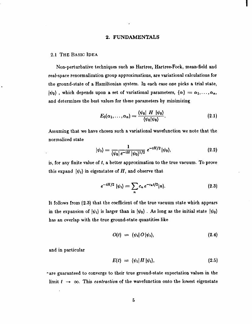
ground-state energy density to order t ‘I. In Fig. 2 we contrast the results ob-

tained by directly forming diagonal Pad6 approximants to the energy density, to

the results obtained by forming off diagonal Pad6 approximants to the derivative

of the energy density and then integrating. We also plot both the behavior of

the Taylor series in the same range and the exact answer. In figure 2 we display

all of the diagonal Pad& which can be formed with our data, and it is clear their

- convergence to the exact answer is fairly slow. This should be contrasted with the

single curve which shows that many of the off-diagonal Pad&s agree with one an-

13

other and converge rapidly to the correct result. Of the integrable approximants

which correspond to calculations carried out to order t7, the 1-5 and 2-4 Pad&s

best approximate the exact answer; i.e., &IS = -43982 and &21 = -.441892,

versus &=a& = -. 44315. The fractional errors for these two case are .75% and

.27% respectively; this should be compared with Anderson’sI calculation of this

quantity in the spin-wave approximation which is on the order of 4% .

Note that in this example the wavefunction I$o) had no variational parameter

associated with it. We will now turn to a second example in order to see how the

method works when there is a variational parameter to play with.

4. THE l+l-DIMENSIONAL ISING MODEL

4.1 THEMODEL

The Ising Model in 1 + 1 dimensions has long been used to compare different

computational techniques. It is defined by the Hamiltonian

H = -Ca.(i)-xCcl,(i)a,(i+l). i i

Our mean-field (Ml?) variational state is a product state

Iti01 = n lej, 4j)

i

(4-l)

(4.2)

where the single site states lflj,#j) are defined in terms of eigenstates of the

operator a=(j) to be

lej, 4j) = COS( % ej) 1 a,(j) = 1) + e’+ Sin( 1 ej) I a,(j) = -1) . (4.3)

If we choose 8 and 4 to be constants, independent of the point j, it follows that

t =(bz) = cos e

x =(4 =sinec0s4 (44

Y “kd = sin Bsin4

14

The MF approximation amounts to

WOW I$o) = -v(t + xz2) . P-5)

Note, that y does not appear here and so must be chosen to vanish (which also

means 4 = 0) in order to minimize (4.5) . Minimization of (4.5) with respect

to 0 gives a disordered phase (Z = 0, z = 1) for 0 5 X 5 l/2 and an ordered

phase with a broken symmetry (z # 0) for X 2 l/2. It is known from the exact

solution to this model that the model has a second order phase transition between

these phases located at X = 1. This differs by factor of 2 from the location of

the phase transition predicted by the mean field approximation. In addition to

missing the location of the phase transition the mean field approximation also

fails to give correct critical indices, and only gives a good approximation to the

energy density for X > 1, i.e. deep within the ordered phase.

4.2 THECONTRACTIONOPERATORCALCULATION

Applying our method we find the following first few terms of the perturbative

energy density by calculating the connected matrix elements of H

&PI Taylor = -(z + Xx2) - t[1- t2 - 4Xx22 + X2(1 + 2x2 - 3z4))

+h t2 [--2(z3 - z) - X( 18z2x2 - 4x2 - 2y2)

- X2(3622’ - 16.~~ - 42) - X3(202’ - 24x4 + 4x2)] . V-6)

It is interesting to note that y dependence shows up for the first time in the Xt2

term and is quite insignificant. For all practical purposes one may choose y = 0.

This continues to be true even to the next few orders in t.

Using (4.6) one can evaluate the l-l Pad6 approximant. This alone causes

*a considerable shift of the critical point. However, in order to do better, we

would like to compute higher PadC approximants. To avoid the complexity of

15

a hand calculation we again turn to the computer in order to evaluate the de-

sired connected matrix elements. As before this is done by computing connected

coefficients for a theory defined on a finite lattice. In what follows we work to

order t6 and therefore must compute (H’)‘. This means that for our numerical

calculation we work on a lattice with eight sites. The computation was carried

out for various values of the parameter 8; the resulting Pad6 approximants are

studied for fixed t as functions of 8. However, before discussing the results of

these computations there is an important technical point which should be made

which relates to the question of determining the range in t for which our Pad&

can be expected to converge.

For the Hamiltonian defined in (4.1), the parameter X is taken to range over

the region 0 5 X 5 00. A problem which arises at this juncture is that we

compute an approximation to E(t) by terminating a Taylor series at a finite

order in t, hence we do not expect the Pad6 approximants formed from this

series to converge for the same range in f for all values of X. The problem is to

find a way of resealing t so as to minimize this effect. We observe that for X >> 1

the Taylor series to order t”, which consists of terms up to order X”+l, diverges

strongly as X ---+ CO. This can be avoided if we rewrite the Hamiltonian, H, so as

to compactify the range of the coefficients; e.g., use a Hamiltonian of the form

H(a) = - cos a a,(j) + sin d a=( j)u,( j + 1) I . (4.7)

In fact, it is only necessary to use H(a) in the contraction operator, and con-

tinue to evaluate all expectation values as before. The precise way in which we

implement this procedure is to let cos Q = l/d-, sin cu = X/X/~ and

define &(f, f?) to be

V-8)

I For fixed t the functions E (t, 0) provide a t9 - dependent upper bound upon

the true vacuum energy. For a fixed value of t we obtain a best bound by

16

I

minimizing E(f, e) with respect to 8. In this sense, the functions E(t, 0) computed

for a fixed value of t play the role of efiecfive potentiala, and we will refer to

them as such. Note that since we do not compute the functions &(t, e) exactly,

but attempt to reconstruct them using Pad6 approximants, the functions we

plot are not necessarily true bounds. In particular, these potentials are reliable

guides to the location of the true minimum in 8 only to the degree in which the Pad6 approximants have converged. For this reason the way in which we

extract information from our calculation is to compare the curves obtained by

constructing various Pad6 approximants. We define the range of 8 for which we

can trust these effective potentials by requiring several Pad6 approximants to

agree. Examples of effective potentials are presented in figures 3-6.

4.3 DISCUSSION OF RESULTS

Figure 3 displays results obtained for a value of X deep in the ordered phase.

The uppermost dashed curve is &(O, e), which corresponds to the familiar Hamil-

tonian mean-field calculation. The three curves which appear below it correspond

to effective potentials [(l, e), E(3,e) and &(5,0) respectively. Solid lines repre-

sent curves obtained by integrating the O-5 Pad6 approximant to d&(t, B)/df, and

points signify values obtained by integrating the l-4 Pad6 approximants. Differ-

ent symbols have been chosen to indicate the results of the 1-4 Pad6 approximant

for the three different f values. This was done in order to make it easy to see

what is happening when the O-5 and l-4 Pad6 approximants no longer agree with

one another. Obviously, for figure 3 this is completely unnecessary.

Figure 3(a) exhibits the behavior of the various effective potentials over the

entire range in 0, and figure 3(b) h s ows what these potentials look like when they

are magnified to more clearly exhibit the structure of the results in the region

of the minimum. These pictures are typical of the behavior seen in the region

*of X > 1.5. In this region the Pad& agree with one another to high precision

and the location of the minimum of all of the effective potentials is quite close

17

to the value obtained from the simple mean-field calculation. The actual best

values of the energy density,however, become increasingly accurate for larger

values of t. The interesting feature of this particular class of curves is the way

in which the effective potentials change as we go to larger values of f. Figure 3

clearly exhibits the fact that the greatest improvements in the estimate of the

vacuum energy occur for trial states which lie far away from the true eigenstate,

and that the total variation of the estimate of the energy density over the entire

range in 0 gets progressively smaller. This is just what one would expect if our

approximation is working correctly, since the result one would obtain for 1= 03

should be the completely flat lower dot-dash line, which is simply a plot of the

exact ground-state energy density for this value of A.

Turning to figures 4(a) and 4(b) we see a much more complicated situation.

Once again, the dashed curve is the f = 0, or mean-field, effective potential;

. and the three curves lying below it give the effective potentials corresponding to

t= 1,3 and 5 respectively. In this figure we see that the O-5 and l-4 t = 5 Pad6

approximants strongly disagree with one another for 8 < 1. This same sort of

disagreement would have been seen in the picture for X = 10 had we plotted

potentials for t’s greater than 5. Presumably, the extrapolation to large t values

would be more stable if one calculated to t8 or t”. This conjecture is supported

by IO-site calculations carried out for a much smaller set of 0 values.

The most striking feature of the curves shown in figure 4 is the enormous

disagreement between the 1 = 5, &5 and l-4 Pad6 approximants for t9 < .5. In

fact the O-5 approximant undershoots the exact energy. As mentioned previously

this signifies the breakdown of our approximation since we know that the exact

effective potential must be an upper bound on the ground-state energy density

for all values of t. From this we see a typical feature of all the calculations, one

Pad6 approximant can be very inaccurate for a range of t and 8, however com-

* parison of several Pad& usually allows us to resolve any ambiguity. Figure 4(b)

exhibits the complicated structures that can occur in any one Pad6 approximant.

18

Note that a reliable estimate of the energy density comes from the point where

the various approximations agree. Had we plotted effective potentials for more

values in the region 0 2 t < 3 we would have seen that the minimum for each

of these functions would be contained in the interval 1.19 < 0 < 1.4. When the

curves split apart the different approximants develop secondary minima. When

this starts to happen one has no reliable way to choose among them. The most cautious approach in this event would be to limit the value of t which one uses

to be less than or equal to the first t value at which the splitting occurs. Inspec-

tion of figure 4(b), h owever, shows that one can be somewhat bolder. Namely,

one can follow the minimum through increasing t values, then choose the best

approximation for larger t-values to be the value of E(t) at the point at which

the various Pad&s continue to agree. In this way, one is able to reliably extend

the calculation to higher values of t than the straightforward approach would

allow. Note, that in figure 4(b) the best point according to this criterion is a

local extremum for some of the Pad& .

Figure 5 exhibits the same set of curves for the critical value X = 1. Now, if

we follow the minimum in through increasing values of t we find that the reliable

region corresponds to 8 5 1. There is nothing particularly striking about these

curves. The only point worth making is that for t < 5 the minimum occurs for a

non-zero value of 8; hence, this calculation incorrectly predicts the critical point

of the theory to be below 1.

The last set of effective potentials diplayed in Fig. 6are typical of the region

.5 5 X 5 .9. We see that for t 2 3 the minima of the various effective potentials

all move to e = 0. In fact, more careful study shows that if we limit ourselves to

f= 3, then the phase transition occurs for X - .9. Since we know that the mean-

field transition occurs at X = .5, the minimum of all Pad& must be at 8 = 0 in

the region 0 2 X 5 .5. As before, the values of E(t) at the minimum improve with I increasing t. Considering that we have only computed our expansion to order

ts, we feel that these results represent a significant improvement over mean-field

19

results for a modest effort. This improvement is made much more striking if we

compare these results to what is obtained by using more complicated block-mean

field or real-space Hamiltonian renormalization group techniques; these methods

require one to work very hard to get results which are not this good.

Having discussed the various effective potentials, we will now explain how we

obtained our values for the ground-state energy density, magnetization, etc.. In

figure 7 we exhibit the energy density obtained from the 1-4 Pad& evaluated for

t = 3. The choice of the 1-4 Pad6 versus the O-5 Pad6 is completely arbitrary,

since for this value of t the difference between the two functions at the minimum

is on the order of a few times lo- 4. Obviously, errors of this magnitude are not

visible on the plot shown in figure 7. It is obvious that the agreement between

this calculation and the exact answer is quite good. In fact, over most of the

range 0 ,< X 5 00 the relative difference between our calculation and the exact

’ answer is on the order of 10W4, and it grows to 4. lOa in a very narrow region

surrounding the point X = .9. This small discrepancy shifts the singularity of

the second derivative of the energy density (i.e., the specific heat) from X = 1 to

x N .9.

The last two curves are plots of our computation of the magnetization; i.e.,

the expectation value of the operator c(az(j))/V computed according to equa-

tions (2.11) (2.12) and (2.13). The crosses in figure 8 corresponds to the values

of the magnetization computed for asymptotic t, i.e. values of t for which the

magnetization has become a constant. Since the O-5 and 1-4 Pad&s agree with

one another to an accuracy which would not be visible on the plot we do not

bother to indicate which is plotted. The solid curve shown in figure 8 is a plot

of the function

.

which is to be compared to the dot-dash curve which is the exact magnetization

20

as a function of X i.e.

+ x(uJj)) = (1- (1/X)2)125w i

(4.10)

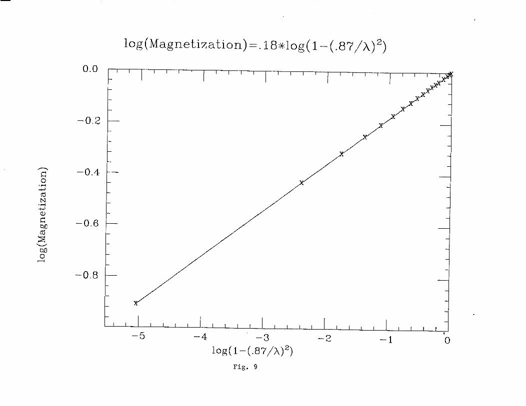
The crosses in figure 9 present the same data, except that we are plotting

log M(X) versus the variable log (1 - ( $I)2). The solid curve is a straight line of

slope .18 chosen to pass exactly through the point in the lower left hand corner

of the graph. It is clear from this graph that it fits a power law of the type (4.9).

While the results presented in this section are by no means in perfect agree-

ment with the exact answer for the 1+1-dimensional Ising model the reader

should recall that they are to be compared to the results of the mean-field ex-

pansion which predicts a phase transition at A, = 0.5 and a magnetization,

M(X)MF which is given by

q%fF = (l-(g-t (4.11)

By computing out to sixth order in t we are able to significantly improve these

predictions in a systematic way.

21

5. TWO PARAMETER EXPANSIONS

5.1 THECONNECTIONTOPERTURBATIONTHEORY

The contraction technique we have introduced is based upon expanding in a

parameter t which does not appear in the Hamiltonian. Therefore, it is applica-

ble even when there is no identifiable small parameter which can be exploited to

develop the more familiar perturbation expansion. Nevertheless there are situa-

tions, such as in the case of the 1+1-dimensional Hamiltonian Ising model, where

such an identifiable parameter does exist and so one is tempted to ask how our

method relates to more familiar techniques. This section has two purposes: first,

we will establish the precise connection between our expansion and the usual per-

turbative expansion; second, we will indicate the way in which one can exploit

this connection to simplify the problem of computing connected coefficients for

a class of interesting problems.

Begin with a Hamiltonian

H=Ho+xV (5.1)

where x is to be identified with the small parameter appearing in the usual pertur-

bation expansion. The operator Ho is referred to as the unperturbed Hamiltonian,

and its complete set of eigenstates will be denoted as I&), with eigenvalues E”,.

In particular, the lowest eigenstate of Ho will be denoted by 140). For the case

of the Ising model discussed in the preceding section x is to identified with X or

l/X depending upon whether we are considering the weak or strong-coupling ex-

pansion. Since the connected coefficient of the term of order t” in our expansion

for the ground-state energy density is obtained by computing expectation values

of (Ho + xV)“+l, it is obvious that each term of order t” is a polynomial of order

n + 1 in the parameter x. Hence, it follows that our series can be rewritten as

E(f) E E(x, t) = (Ho) + 2 (-t)“+px”+l (gV”+‘) c, nsao (n + PI!

(5.2)

22

where the symbol (HiV”+‘) ’ stands for the appropriate sum of connected matrix elements. The next question is, how must this series be resummed in order to

obtain the usual perturbation expansion. To do this in the most straightforward

manner we will present the discussion in a way which directly parallels the usual

development of a perturbation expansion.

To establish the connection between our contraction formula and perturba-

tion theory in x we consider the operator eetHi2 applied to the lowest eigenstate

of HO, 140); i.e., consider ratios of the form

For now focus on the energy E(t) which can be written as

E(t) = (401 IA+ MO) (401 e-tH 140) * (5.4)

In analogy with the construction of the interaction representation we define the

operator

F-5)

This is not a unitary operator, as in the Schrijdinger problem, however it does

obey the same group property

Wl, t2w2, t3) = w, t3).

The operator U(t) E U(f, 0) satisfies the differential equation

w 0 -- = xV(t)u(t) dt (5.7)

* where

V(f) = etHo ViBtHo.

23

w4

(5.8)

The solution to (5.7) is the time-ordered exponential

-z j V(r)dr U(t) = Te 0 . (5.9)

Expanding U(t) in x one obtains a power series in x whose coefficients are

complicated functions of f. It follows from (5.7) that the function E(t) is simply

E(t) = (~olHe-‘H MO) = JJO + Jtiol V(ww l$o) (4ol ctH MO) O ($01 W) 140) (5.10)

Substituting the Taylor expansion for U(t) in both the numerator and denomi-

nator of (5.10) we obtain an expression for E(t) which suffers from the the same

problem addressed by Theorem I, namely the coefficients of x” diverge as V”+l.

The solution of this problem proceeds as before; we observe that the ratio (5.10)

must, term by term as a power series in x, be free of all volume divergences.

Hence, we know that

(hl WW) 140) (4olw)l~o) =.c,7

O” (-‘I” (vn+l(t)) e

= (5.11)

where each connected matrix element appearing on the right hand side of (5.11) is

proportional to one power of the volume. Once again, connected matrix-elements

are defined recursively by

(V”+‘(t))’ =@ol W)Tt/t V(W)” 140) 0

“+1-P(t)) “(#ol T(/’ V(T)d+’ I&). 0

(5.12)

We have now established two equivalent expansions for E(x, t); namely,

e E(x, f) = I$ + x c O” k$” (v”“(t)) c = 2 9 (H”+‘(x)) ‘. (5.13)

n=O * n-0 ’

24

Expanding (V”+‘(t)) as a power series in f, and (H”+‘(x)) as a power series in x we obtain the double power series expansion of equation (5.2). Now, however,

we are able to identify the connected matrix element (HgVn+l)e either as the

coefficient of f”+P appearing in the expansion of (V”+‘(t)) ‘, or as the term of

order x”+* appearing in the coefficient of f”+p in our original t-expansion.

We now argue that by inserting a complete set of intermediate states into

(5.11) using the recursive definition (5.12) and taking the limit t + co we obtain

the familiar perturbation expansion. To see how this works consider the first few

terms of the expansion; i.e.,

E(x, 4 = G + 4401 v MO) - X2”S0 l(&l v l4”)l 2 1 - ef(g-EO,)

E$ -$I +-- ! t5-14)

where we have inserted a complete set of intermediate states and explicitly car-

ried out the necessary integrations over the r-variables. It is this integration

which converts an expression free of energy denominators into one with such

denominators. Taking the limit t + 00 we see that the decreasing exponential in

the term of order x2 vanishes leaving us with the familiar result of second-order

perturbation-theory. Note that expanding this term around t = 0 one finds that

it starts like f , as it should, and that the energy denominators disappear, as they

must, when we expand this result as a Taylor-series in t.

5.2 EXPLOITING THE DOUBLE EXPANSION

Note, that it is often true that V connects 140) to one, or at most a small

number of other eigenstates of Ho. When this happens then it is quite simple to

compute the analogue of (5.14) directly and use it to generate the t-expansion.

From a computational point of view this observation can greatly simplify the

task of computing connected matrix elements for the general t-expansion.

A more important point relating to the general structure of the two parameter

expansion has to do with the general question of convergence, both of Taylor

25

series and sets of Pad6 approximants. On the one hand, the general f-expansion

amounts to first summing over all orders in z corresponding to the same power

in t and then constructing Pad&s to the resulting Taylor series in t. On the other

hand, perturbation theory corresponds to summing over all terms multiplied by

the same power of 2 in order to obtain a sum of decreasing exponentials in t; then,

taking the limit t --* 00. Which of these procedures can be expected to work best obviously depends upon the region of z and t under consideration. In the region

x << 1, where we might expect perturbation theory to be rapidly convergent, it is

in general preferable to use the Taylor-expansion in z, leaving the t-dependence

in the form of decreasing exponentials. In this case one is not exploiting the

contraction approach at all. However, when z is large and simple perturbation

theory in x can no longer be trusted, the contraction approach comes into its

own. In addition, perturbation theory is usually only an asymptotic series; the

fact that the contraction approach is expected to converge gives us a prescription

for resumming the finite t perturbation expansion in order to render it more

convergent. We will discuss questions of convergence in chapter 7.

Another point is that there is no reason why the parameter t appearing in

our general formulae cannot be replaced by a complex parameter z, so long as we

take the limit X(z) + 00. This would correspond to the usual Gell-Mann Iowl’

expansion, if we take matrix elements between two different states defined by

taking t = t(~ + ;) and z* = t(c - i). The next section is devoted to the theory of such expansions and we will delay discussion of this point to that section.

Finally we would like to point out that the perturbative technique combines

with the variational approach in a straightforward fashion. The trick is to replace

the variation of the parameters in I$c) by an equivalent variation of parameters in

a “shadow-Hamiltonian”~-Q1 i.e., an unperturbed Hamiltonian HO whose lowest

eigenstate is I&). This is useful since in a general case it is easier to change

-parameters in the Hamiltonian than in the wave-function. Another virtue of this

approach is that it is often easier to guess, on physical grounds, what operators

26

(or order parameters) should be varied in Ho; whereas it may be quite difficult

to find the correct direction to choose in Hilbert-space. Subtracting the shadow-

Hamiltonian from the true Hamiltonian we obtain a separation of the type of

(5.1), however in general this no longer leads to a simple perturbation theory

and can prove cumbersome in practice. The decision of whether to use the

perturbative technique or directly calculate the t-expansion should be made on

the basis of the problem to be studied.

6. BI-STATE CONTRACTION SCHEME

To this point we have focused on a contraction scheme based upon taking

diagonal matrix elements of operators. This method is powerful and easy to im-

plement for a wide variety of Hamiltonians; nevertheless, there are problems for

which it is desireable to be able to compute with off-diagonal matrix elements.

For example consider the problem of computing the ground-state energy den-

sity or string-tension for a non-abelian lattice gauge theory. For a non-abelian

theory there is only one gauge-invariant mean-field state which can be written

down, i.e., the infinite coupling vacuum. If we restrict our analysis to diagonal

matrix elements and product wavefunctions, then we lose the ability to introduce

a variational parameter. As we have already seen, however, without a variational

parameter we give up a considerable amount of accuracy. A variational parame-

ter can be introduced by using a mean-field wavefunction which is non-trivial but

such a wavefunction is no longer gaugeinvariant; hence, we are unable to trust

computations of the string-tension, etc., obtained in this way. It is therefore

highly desireable to develop a scheme which allows us to introduce a variational

parameter without abandoning the explicit gauge-invariance of the computation.

The technique which we will now discuss, which exploits two states and computes

off-diagonal matrix elements, has this virtue. The application of this approach

-to the study of lattice gauge-theories is currently under investigation, and will be

presented elsewhere. We will show here that this bi-state computational scheme

27

is useful whenever we can construct a good approximation to the vacuum wave-

function of a Hamiltonian system for two widely different values of the coupling

constant, because in that case it allows us to construct an expansion about both

points simultaneously. As an example of this aspect of the scheme we will show

how it can be used to construct an explicitly self-dual series for the energy density

of the Ising model in 1+1 dimensions.

6.1 GENERALFORMALISM

Begin by considering two different states I&) and 1x0). Using either of these

states by themselves we can construct the improved states I+,) and Ixt), and use

them to construct two independent approximations to the vacuum energy; i.e.,

-tH MO)) E+(t) = ($+I H (?Jt) = -d(ln($ol;t ,

and

-tH 1x0) ‘%(t) = (xtl H Ixt) = -@‘(X0$

,

(64

(f-9

both of which have the true vacuum energy as an asymptotic limit. Next consider

the expression

4l4$ol ctH lxo)) Q%(t) = - dt - (6.3)

We will refer to this as the bi-state contracted energy. As a matter of convenience

we will assume that I$Jo) and 1x0) have been chosen so that E+Jt) is real. In

contradistinction to E+ and EX, (6.3) is not, by itself, an upper-bound on the

vacuum-energy. It is, however, guaranteed to converge to the true energy in the

limit t + 00. To convert this information into a form which does provide a

bound we make use of the Schwartz inequality a

I(+01 ewtH IXo)12 5 ($01 eDtH I$o) (XoI e-tH Ixo). (64

28

Integrating (6.1), (6.2) and (6.3) with respect to t we can solve for the various

quantities which appear in (6.4). For example, we find

(qol fFtH - j &(r)dr

I?W = (tool$o)e 0 , (6.5)

and analogous expressions for the other matrix elements of eatH. Inserting them

into the Schwartz inequality leads to the result

t

t 2X J

E&)d7 + In ($01 tDo)(xol x0) >

IWol xo)12 - / W&) + ~x(W~ > 2tE”ae, - (6.6)

0 0

which tells us that the lefthand side of (6.6) is an upper bound upon the true

vacuum energy. In addition, it tells us that this quantity is always greater than

or equal to the minimum diagonal approximation to the energy. Having recast

the bi-state computation into the form of an upper bound we may exploit this

bound by varying the left-hand side of (6.6) to fix the choice of the parameters

in I&) and 1x0). Note that it is necessary to integrate to large t-values if one

wishes to render the role of the logarithmic term in (6.6) negligible. To do this

reliably, however, will generally require computation of many connected matrix

elements. If one can extrapolate to large t one may apply the criterion of a

stationary point in parameter-space to 2x1 &Jr)& directly, although it is not

truly an upper bound. In practice there should not be much difference between

these two methods for reasonable t values.

The Schwartz inequality (6.4) can also be used to obtain

Ih( 2 lbhl H Ixt)l. (6.7)

-The right-hand side is yet another expression that tends to the desired asymptotic

limit; which, however, cannot be exploited since our treatment of the cancellation

29

of volume factors in the t-expansion does not apply to this quantity, whereas it

does apply to E+,(t). We should point out that since our proof of Theorem I

did not make use of the state appearing on the left and right hand sides of the

expectation value, and in fact did not even require that they be the same state,

the result of Theorem I generalizes to the bi-state situation. Hence, all of the

tools which we have developed carry over directly. The only change which must

be made is that there is an arbitrariness in the definition of connected matrix

elements having to do with the normalization one chooses for the states I+c) and

1x0). Since these normalizations are arbitrary one may choose, without any loss

of generality,

(tiolY4J = 1

($01 x0) = 1. (6.8)

In this case, all definitions of connected matrix elements are as before except that

all operators are to be taken between (Qal and 1x0).

6.2 APPLICATION To THE ISING MODEL

As an example of the application of the b&state method to a specihc problem

let us consider our previous example, the Ising model in l+l dimensions. In this

model we know the form of the vacuum wave-function at opposite extrema of the

coupling X (i.e. strong and weak couplings), the problem is to construct a way

of simultaneously interpolating from both ends of parameter space to the region

X = 1. This kind of extrapolation is just what the b&state scheme does for us.

If we let I&) and 1x0) be the exact strong- and weak-coupling groundstates,

respectively, we have a systematic procedure that allows us to approach the true

vacuum throughout the entire range of couplmgs. More specifically we choose these states to satisfy

a

~3b) MO) = l?bo) f-4.) 1x0) = 1x0) (6.9)

30

It is obvious that I&) is the vacuum of the Ising Hamiltonian

H = -c a3(i) - X ~al(i)al(i + 1) i i

(6.10)

in the limit X = 0; and 1x0) is one of the two degenerate vacuua in the limit x = 00.

Perhaps the most amusing feature of this application of the bi-state technique

is that the t-expansion which is generated has the very interesting property of

being term by term self-dual. To our knowledge this is the only systematic

expansion which exhibits this discrete symmetry of the exact theory. For non-

experts we point out that the duality transformation for the Ising model in l+l

dimensions amounts to replacing the point variables u by another set of Pauli

spin-matrices r associated with the links of the lattice. If one denotes every link

by the point to its left, the relations between these two sets of operators should

be 03(i) = 71(i - 1)71(i)

73(i) = Ul(i)Ul(i + 1)’ (6.11)

It follows that H(X) turns into AH@-‘) for the onedimensional system in which

the links (which are dual to the lattice points) form an equivalent system to the

one we started with. The duality relation should hold for every energy level of

the Hamiltonian

E&l) = XE&+). (6.12)

Performing the duality transformation on I+u) and 1x0) one finds that they

interchange their roles. Since in this basis all the matrix elements that we need

will be real it follows that they will automatically be self-dual; thus guaranteeing

that the resulting energy-function will obey (6.12) .

In our treatment of the Ising model as a bi-state calculation we fixed the two

states I@o) and 1x0), and therefore have no variational parameters with which

31

to play. As a result the energy, calculated to the same order in t as in chapter

3, is less accurate over the entire range in X. There, the biggest error was on

the order of lo- 3 at the phase transition, and on the order of lo-’ elsewhere;

here, on the other hand, the relative error is on the order of 10e3 throughout.

Another feature of this result is that to this order in t the calculation does not

show a phase-transition. The second derivative of the energy-density, however,

does peak at X = 1, the self-dual point. This means that consecutive higher

orders in t are required to slowly build up the singularity associated with the

second-order phase-transition at the correct point.

6.3 GAUGE THEORIES

We expect the bi-state calculational scheme to be particularly useful for local

gauge theories. Characteristically such models can be easily solved in the strong-

coupling regime, but they are very difficult to tackle in the weak-coupling regime,

which happens to be the one of interest. The difficulty arises because local gauge-

invariance has to be maintained by the vacuum wave-function. This rules out

a mean-link ansatz, that could otherwise be appropriate for the weak-coupling

region unless it is properly projected onto its gauge-invariant part. While one can

formulate a gauge-projected mean field calculationl1ol it is in general prohibitively

complicated to implement. The bi-state approach manages to allow us to use

non-trivial product wave-functions without going through such a complicated

procedure. If one uses the strong-coupling wave-function for I&), one is free to

use any state for 1x0) without worrying about its gauge properties. The fact that

I&) and H are gauge-invariant, guarantees that only the gauge-invariant part of

1x0) will be involved in the calculation. This provides an enormous simplification

of the problem.

A particularly straightforward series is developed if one uses a mean-link state

‘for 1x0). In this case, since both I$o) and 1x0) have no link-link correlations, we find that connected diagrams are still ones which touch in configuration-

32

space. With this ansatz the bi-state approach allows for calculations in the

weak-coupling regime that were up to now unique to strong-coupling perturbation

theory.

6.4 COMPLEX t

Finally let us return to the remark that we are free to choose the parameter

t to be a complex variable t. In particular we could choose z to be t = (i + ~)t,

where epsilon is a small positive real number. In this case the state

I$(%)) = e-qc+qH Itjo) (6.13)

becomes the usual time dependent state of the Schroedinger representation in the

limit t 4 0. Now let us recall that the usual formulation of perturbation theory

for Green’s functions, etc. involves the computation of time-ordered products

of fields between states I@(t)) and 1+(-t)) in the limit t + 00. Clearly, this can

be thought of as an example of a bi-state calculation take between states 1$(z))

and hW)h h w ere z is taken as indicated and the limit E -+ 0 is to be under-

stood. Aside from the fact that it is always interesting to be able to establish the

connections between different approaches, this observation is interesting because

it raises the question of whether or not this formalism can be used to calculate

scattering amplitudes as well as energy levels. It also raises the question of if the

series in the complex variable z and perturbative parameter z can be rendered

even more convergent by resumming it in a manner which is different from the

one we have used in this paper.

33

7. ANALYTICITY OF THE t-EXPANSION

Up to now we have discussed the t-expansions as if E(t) and Z(t) are guar-

anteed to be analytic functions of t, independently of the initial states I$e) and

1x0). This is not necessarily the case. If one starts with a wavefunction which

is a sufficiently bad approximation to the true ground-state of the system, then

Z(t), etc. may be non-analytic. If this occurs it will affect the convergence of the

Pad6 approximants, and so it is important to be aware of this possiblity.

The simplest way to see that this can happen is to expand the state I$J~) in

a complete set of eigenstates of H; i.e.,

Wo) = Ccnln) n

and rewrite the norm Z(t) as

Z(t) = (+ol CtH I$o) = c c~c,e-tEm n

= c

e-tEte+s(E”) . ?

Em

(7.1)

P-2)

SW”) = log(~c~c,) is the sum over all eigenstates of H having energy En.

This procedure maps the problem of computing Z(t) into the problem of com-

puting the partition function for a classical system at temperature l/f, with

entropy S(&). Thus, if this equivalent classical system exhibits a finite temper-

ature phase transition, then quantities like E(t) will be non-analytic in t; higher

derivatives of this function will exhibit singularities. Obviously, if the en’s vanish

sufficiently rapidly as a function of E, there will be no problem, the extreme case

being that all but a finite number of the en’s vanish. Our discussion of theories

a in one spatial dimension was protected from this problem because in one spatial

dimension there are no phase transitions at finite temperature.

34

We hasten to emphasize the fact that while this is a possible problem, this

lack of analyticity only manifests itself for some choices of a trial wavefunction;

in general, it can be avoided if one chooses a wavefunction with some care.

Presumably, this sort of effect will be signaled by the fact that several Pad6

approximants will exhibit singular behavior at the uamc value of t .

We will now discuss several examples and present a criterion for telling when,

within a class of trial wavefunctions, one may encounter non-analyticity in t. This

criterion is a conjecture and certainly doesn’t have the status of a theorem, but

we believe that it generally provides a guide to when we can get into trouble.

Our basic aim is to use this criterion to compare lattice spin systems and lattice

gauge-theories. We will argue that the spin system can present some difliculties

as soon as the dimension of the spatial lattice is greater than or equal to 2. On

the other hand, the non-abelian lattice gauge theory can be expected to present

no particular difficulties if the spatial dimension of the lattice is less than or

equal to 5. We reemphasize that this argument does not mean that one cannot

use the t-expansion to analyze spin systems in two and more dimensions; rather,

it says that if one does, one has to be more careful in choosing the starting

wavefunction for a spin system than for a gauge theory. We conclude with the

example of similar problems which can be encountered for a quantum mechanical

system with a single degree of freedom. This example is included in order to show

how changing the wavefunction can avoid difficulties.

7.1 SPIN MODELS

Consider a higher dimensional spin system of the Ising type; i.e., theories

defined by Hamiltonians of the form

H=x -u,(j) - xa,&$ + ii) 1 . 3 (7.3)

- As in the l+l dimensional Ising model, these theories exhibit ordered and disor-

dered phases. The completely disordered phase corresponds to the case X = 0,

35

and the completely ordered phase to the case X = 00. We denote the vacua of

theX=OandX = 00 Hamiltonians by 140) and l&,0) respectively. As in the

l+l dimensional theory, we can use the general class of mean-field wavefunctions

which depend on the single parameter 0 to interpolate between 140) and I&).

We now ask what happens if we attempt to use the contraction technique

to construct l&,) starting from I&-,). More precisely, we wish to compute the

t-dependence of the function

Z(t) = (SOle-tHl#O), (74

where the state 140) is defined to be the state for which

Qwo) = MO)* (7.5)

In effect we want to know if we get the correct ground-state energy, etc., using

that wavefunction which lies furthest from the true vacuum. Our conjecture

is that if this works, then we can expect our general calculation to be free of

trouble. Conversely, if this calculation exhibits a phase transition in t, then we

can expect to have problems.

Note that the state, which is an eigenstate of all a,(;) with eigenvalue 1, can

be rewritten in terms of eigenstates of cr=(:) as

IW = qJV[l --+I+ I -I], 1 a (7.6)

where V stands for the number of lattice sites. This product state is, up to the

normalization factor of (l/fi)v, j us a sum over all of the eigenstates of the t X = cc Hamiltonian

ti = - c u&rz(~). V-7) (:,?I

36

Hence, we see that with this choice of 140)

which is immediately recognizable as the classical Ising model in d-dimensions

(where d is the spatial dimension of our lattice).

It is easy to show that in the case of one spatial dimension

Z(t) = (cosh(t))v (W

and

which explains our interest in

that this function is analytic

of the fact that there are no

E(t) = tanh(t); (7.10)

being able to Pad6 functions of this type. The fact

for alI finite values of t is just a specific example

phase transitions at finite temperature in one di-

mension. If the spatial dimension of our lattice is 2 or greater, however, then we

know that the classical statistical mechanics problem does exhibit a phase tran-

sition. Hence, for these theories if one uses the X = 0 wave-function to calculate

physical quantities one can run into problems with analyticity in t. Presumably,

a variational ansatz, is capable of avoiding such problems.

Note that if one chooses for I&) the wavefunction

and chooses for a the X = 0 Hamiltonian

(7.11)

37

the same sort of argument indicates that there is nothing to worry about. In this

case we obtain E(t) = tanh( t), as in the case of the one dimensional theory, and

everything is completely analytic. Apparently, the difference between these cases

is that when starting from the disordered vacuum the contraction operation has

no way of choosing between the two possible ordered vacua of fi. Obviously, if we

start from one of the two ordered states and try to contract onto the single totally

disordered state the situation will be better. In any event, the lesson we wish

to leave the reader with is that one can, if one is not careful, run into problems

with analyticity in t; however, simple modifications of the starting wavefunction

can in general avoid these problems.

7.2 GAUGE-THEORIES

Let us now apply the same argument to the case of a lattice gauge theory.

In this case the basic variables, the fields of the model, are continuous functions

taking values on a compact Lie group. We will show that for these gauge the+

ries a t-expansion built upon the simplest strong coupling wav+function can be

expected to generate a non-analytic function of t when the spatial dimension of

the theory is greater than a critical dimension, d,. Fortunately, we will find that

for an abelian theory d, = 4 and for a non-abelian theory d, = 5. Thus, for

the theories of physical interest we do not expect to have any difficulty with the

application of our methods in their simplest possible form.

Consider a lattice gauge-theory defined by a Hamiltonian of the form

H = 4’ c E: - L ~(‘rrcr, + kc.), ha g2 P (7.12)

where 1 stands for lattice links, and p for plaquettes. Choose for It,6c) the wave

function which is annihilated by all of the electric field variables. Following

‘the logic used for the spin models let us analyze the zero coupling Hamiltonian

fi obtained by dropping the E”, term from (7.12). As before this represents

38

the worst possible mismatch between wavefunction and Hamiltonian, and so our

conjecture is that if the Z(t) is analytic in this case it will be analytic for finite

g. Evaluating the norm of the contracted state we obtain

(7.13)

which can be immediately recognized as the Wilson action for a Euclidean lattice

gauge theory in d-dimensions; recall our problem is assumed to be formulated in

d+l space-time dimensions. If the gauge theory under consideration is abelian,

then we know that for d = 4 the theory exhibits a phase transition; hence, we

could expect problems for t-expansion for an abelain theory in five space-time

dimensions. For a non-abelian theory the belief is that the Wilson theory does

not have a phase-transition below d = 5, and so the t-expansion is expected to

converge for all theories in the interesting case of four space-time dimensions.

Hence, we believe that this method will run into no difficulties for the case of a

pure gauge theory in 3+1-dimensions.

7.3 THEANHARMONIC OSCILLATOR

We will now show that one can run into difficulties even when dealing with

quantum mechanical problems of one degree of freedom when the quantum vari-

ables of the problem are continuous and non-compact. To see how this occurs,

and to see what must be done to avoid it, we consider the anharmonic oscillator.

The anharmonic oscillator is defined by a Hamiltonian of the form

H = p2 + z4 . (7.14)

Clearly, in this example we will run into no difficulties with volume factors, so

much of the formalism of connected graphs is not essential. Nevertheless, one

a still has to divide the expectation value of H by the norm of the improved state,

and so the formula is still useful.

39

Let us choose I&) to be a Gaussian wave-function, i.e., the ground state of

some harmonic oscillator shadow-Hamiltonian

.

Ho+0 = 2 IdO

(7.15)

Since w is directly related to the width of the wave-function we see that we may

vary w so as to obtain the best expectation value for

&=I $Wtlrodz. (7.16)

It is a straightforward matter to compute the t-expansion for this problem; unfor-

tunately, the results are quite disappointing since the straight Pade approximants

fail to converge well near t = 0, and so it is difficult to understand how to con-

tinue to larger t’s. The difficulty encountered in this calculation can be easily

understood if we apply our conjecture and study the properties of the Z(t) which

corresponds to contracting an arbitrary gaussian wavefunction using the simpli-

fied Hamiltonian fi = x4. In this case the problem of computing (&I e-” I&)

reduces to the computation of an integral of the form

J e-tZ’e-CVZ2dz (7.17)

which diverges for t < 0. This is the problem which the Pad4 approximants were

trying to reproduce, and since it is an effect due to choosing a bad wavefunction

no clever modification of the PadC prescription will really be able to rescue the

situation.

Clearly, the problem encountered here is simple to solve; one only has to

choose for I+o) a wavefunction which vanishes sufficiently rapidly as z + co.

s This is the route that should be chosen for multi-dimensional models with non-

compact variables where one has to rely on the t-expansion to deal with problems

40

associated with factors of volume. However, it is interesting to note that for

the simple quantum mechanics problem there exists an alternative to choosing

a better behaved starting wavefunction. We will conclude our discussion by

presenting this alternative since it is a useful technique for a class of interesting

problems.

The fact that the Taylor series for the exponential of the Hamiltonian has no

radius of convergence around t = 0 does not reflect on the logic of the contraction

technique; it merely implies that approximation of emtH by a power series in t

is not possible. There is another approximation of the exponential which can be

used in this situation, and that is to approximate it by polynomials, &(t) defined

bY

&(f) = (l- g)y (7.18)

since

,-tH/2 (7.19)

To use (7.18) and (7.19) we approximate the norm of I+!+) by

(7.20)

and hold 6 = t/2n fixed while increasing n. With this prescription the limit

n -+ 00 coincides with the limit t -+ 00.

This approximation has two advantages:

1. Using it in (7.20) yields a positive norm for every value of n.

2. It is free of any singularity in t yet it converges uniformly as n --) 00.

If one computes with this procedure for c s 0.01 and n = 20 one obtains the

- ground-state energy to fifteen significant figures. The convergence is extremely

rapid.

41

This concludes what we have to say about questions of convergence of the

t-expansion, except to emphasize that this is a subject which merits considerably

more study.

ACKNOWLEDGEMENTS

We would like to thank R. Blankenbecler and R. Sugar for helpful sugges-

tions. In particular, it was their insistance that our formalism should allow us to

work between two different states which led to the bi-state method introduced

in chapter 6. We are also indebted to M. Karliner for many helpful discussions.

42

REFERENCES

1) K. G. Wilson, Pbys. Rev. DlO (1974), 2445.

2) J. Kogut and L. Susskind, Pbys. Rev. Dll (1975), 395.

3) G. A. Baker Jr. Essentials of Pack? Approximmts Acacdemic Press

N.Y., 1975.

4) H. A. Bethe, 2. Pbys. 71 (1931), 205.

5) P. W. Anderson, Pbys. Rev. 88 (1952), 694.

6) P. Pfeuty, Am. Pbys.(N. I’.) 57 (1970), 79.

7) M. Gell-Mann and F. Low, Pbys. Rev. 84 (1951), 350.

8) D. Horn, Pbys. Rev. D23 (1981), 1824.

9) H. Quinn and M. Weinstein, Pbys. Rev. D26 (1982), 1661.

10) D. Horn and M. Weinstein, Pbys. Rev. D25 (1982), 3331.

43

I

FIGURE CAF’TIONS

1. Connected diagrams for the Heisenberg anti-ferromagnet up to order t2.

2. Comparison of various ways for using the f-expansion to obtain the

groundstate energy density. The curve marked J!$..~~~ is a plot of the

Taylor series. The curves (l,l), (2,2) and (3,3) are diagonal PadC approx-

imants. Four curves obtained by integrating the (0,4), (1,4), (1,s) and

(2,4) PadC approximants to the derivative of the energy density coincide

with one another on this scale, and all have asymptotic values which are

very close to the exact answer.

3. (a) Effective potentials forX = 10. The curves showing the t=O (mean

field theory), t = 1,f = 3 and f = 5 effective potentials monotonically converge to the exact answer represented by the straight line. Solid

curves correspond to the result obtained from the (0,5)-Pad6 approxi-

mant, and symbols indicate the result of using the (1,4)-Pad&s . The

circles mark the curve obtained from the l-4 Padi! approximation to the

f = 1 data, the crosses mark the l-4 PadC approximation to the f = 3

data, and the sharp-signs denote the results of the l-4 Pad6 approxima-

tion to the derivative integrated to f = 5. (b) Same plots where the

region of the minimum is magnified

4. (a) Effective potentials for X = 1.428. The notation is as in Fig. 3. (b)

This is a magnification of the region around the minimum. Note that

the &5 and 1-4 Pad&s for f = 3,s disagree substantially except at the location of the minimum of the f = 1 curves.

5. Plot of effective potentials for X = 1.

6. (a) Effective potentials for X = .833. Notation as before.Effective poten-

tials for higher f-values have a minimum at 8 = 0, indicating a transition

to the disordered phase has occured.

44

I

7. Energy density from (l&Pad& evaluated at f = 3

8. Linear plot of magnetization versus X . The broken curve is the exact

result, and the solid curve represents a fit to our calculated values by a

function having the same form but with a different exponent and X,.

9. A log-log plot of our results for the magnetization

45

P -

t ’ - 0

l e o- e

3-84 4771Al

Fig. 1

Ener

gy

Dens

ity

0 0 bl

? 09

rtP

. N

l-u* b bl

0 - L I

I I

I

0 0

0 b

k T-

h2

0-l

0 c-

n I

I I

I

-; I

-I I I I I I

dlLL

I I \ I I \ \ \ \ \ \ I 72

-N

I- I I

I I

I I

I I.

I I

I I

I I

I I

I

Ener

gy

I 6 do

6

-A

rL

0,

(, I,,

I

I I

I -4

L I

L I

I I

I I

I I

I

I I

1 I

I

Ener

gy

I E cb

cb

El

b

b

e -!-

I i

I I I I I I I

Ener

gy

0 bl

I I

I I

I I

I 1

I 1

I I

I I

I I

I I

I ‘c

I’?

I

I

Ener

gy

I

- - -

I I

II 11

1

I I

I I

I I

I I

I I

I I

r, f’ \

.

Ener

gy

I F ib

-P

.--

/ ,,

/ ,’

-

Ener

gy

C C b

n

I F e 0

I w

I I

I I

- I

I I

I I

I I

I I

I I

I I

I I

I

-I

I I I I I I I -

I I I

-

/ /

/ /

/

-

. .

. .

P-

C----

i 1

-

Mag

netiz

atio

n

I 0 co

log(

Mag

netiz

atio

n)

I 0 I 0 zu

0 0