Embed Size (px)
Citation preview
RTL implementation of Viterbi decoder
Master’s thesis performed in Computer Engineering
by
WEI CHEN Reg nr: LiTH-ISY-EX--06/3886--SE
Linköping June 02, 2006

RTL implementation of Viterbi decoder
Master thesis
performed in Electronics Systems, Dept. of Computer Engineering
at Linköpings universitet
by Wei Chen
Reg nr: LiTH-ISY-EX--06/3886--SE
Examiner: Professor Dake Liu
Linköpings Universitet
Linköping June 02, 2006


Presentation Date June 02, 2006 Publishing Date (Electronic version) June 02, 2006
Electronics Systems, Dept. of Computer Engineering 581 83 Linköping
URL, Electronic Version http://urn.kb.se/resolve?urn=urn:nbn:se:liu:diva-3886
Publication Title: RTL implementation of Viterbi decoder Author(s): Wei Chen
Abstract A forward error correction technique known as convolutional coding with Viterbi decoding was explored in this final thesis. This Viterbi project is part of the baseband Error control project at electrical engineering department, Linköping University. In this project, the basic Viterbi decoder behavior model was built and simulated. The convolutional encoder, puncturing, 3 bit soft decision, BPSK and AWGN channel were implemented in MATLAB code. The BER was tested to evaluate the decoding performance. The main issue of this thesis is to implement the RTL level model of Viterbi decoder. With the testing results of behavior model, with minimizing the data path, register size and butterflies in the design, we try to achieve a low silicon cost design. The RTL Viterbi decoder model includes the Branch Metric block, the Add-Compare-Select block, the trace-back block, the decoding block and next state block. With all done, we further understand about the Viterbi decoding algorithm and the DSP implementation methods.
Keywords Viterbi decoder, Convolutional coding, Puncturing, Soft-decision, FEC, Error Control System
Language Y English Other (specify below)
69 Number of Pages
Type of Publication Licentiate thesis Y Degree thesis Thesis C-level Thesis D-level Report Other (specify below)
ISBN (Licentiate thesis) ISRN: LiTH-ISY-EX--06/3886—SE
Title of series (Licentiate thesis) Series number/ISSN (Licentiate thesis)
Abstract
A forward error correction technique known as convolutional coding with Viterbi decoding was explored in this final thesis. This Viterbi project is part of the baseband Error control project at electrical engineering department, Linköping University. In this project, the basic Viterbi decoder behavior model was built and simulated. The convolutional encoder, puncturing, 3 bit soft decision, BPSK and AWGN channel were implemented in MATLAB code. The BER was tested to evaluate the decoding performance. The main issue of this thesis is to implement the RTL level model of Viterbi decoder. With the testing results of behavior model, with minimizing the data path, register size and butterflies in the design, we try to achieve a low silicon cost design. The RTL Viterbi decoder model includes the Branch Metric block, the Add-Compare-Select block, the trace-back block, the decoding block and next state block. With all done, we further understand about the Viterbi decoding algorithm and the DSP implementation methods.
1
Contents 1 Background ...............................................................................................................................5
1.1 Introduction ....................................................................................................................5 1.2 Purpose...........................................................................................................................5 1.3 Method ...........................................................................................................................5 1.4 Report structure ..............................................................................................................5
2 Viterbi decoding algorithm .......................................................................................................6 2.1 Overview and introduction.............................................................................................6 2.2 Convolutional coding .....................................................................................................6 2.3 Euclidean distance..........................................................................................................9 2.4 The Viterbi Algorithm ....................................................................................................9
3 Behavior model of the Viterbi Decoder ..................................................................................12 3.1 System Overview .........................................................................................................12 3.2 Data generator ..............................................................................................................12 3.3 Convolutional Encoder.................................................................................................13 3.4 Puncturing Coding........................................................................................................13 3.5 BPSK Modulation ........................................................................................................14 3.6 AWGN channel ............................................................................................................15 3.7 De-modulation..............................................................................................................16 3.8 De-puncturing coding...................................................................................................16 3.9 Viterbi decoding: ..........................................................................................................16 3.10 The Performance Estimation block: .............................................................................17
4 RTL model of the Viterbi Decoder..........................................................................................18 4.1 The Next state ROM: ...................................................................................................21 4.2 The BMU block: ..........................................................................................................23 4.3 The ACS block .............................................................................................................24 4.4 The Trace-back block ...................................................................................................25 4.5 The decoding block ......................................................................................................26
5 Results.....................................................................................................................................27 5.1 Performance of Viterbi decoder with different rate:.....................................................27 5.2 Waveform of RTL implantation ...................................................................................30
6 Discussion ...............................................................................................................................31 7 Future work.............................................................................................................................32 8 References...............................................................................................................................33 9 Appendix.................................................................................................................................34
9.1 Matlab files...................................................................................................................34 9.2 vhdl files.......................................................................................................................49
2
List of Figures
Figure 2.1 a simple Viterbi decoding system Figure 2.2 an 1/2 rate, constrain length 3, convolutional encoder Figure 2.3 the FSM of the example convolutional encoder Figure 2.4 a trellis diagram of example convolutional encoder Figure 2.5 an example of Euclidean distance’ Figure 2.6 the flow chat of the Viterbi decoding Figure 3.1 the block layout of simulation system Figure 3.2 a convolutional encoder for proposed Viterbi decoder Figure 3.3 a rate 2/3 puncture coding Figure 3.4 the constellation diagram for BPSK Figure 3.5 the AWGN channel Figure 3.6 the BER of BPSK modulation in AWGN channel Figure 3.7 he 3-bit soft decisions Figure 3.8 he Viterbi decoding diagram Figure 4.1 the Flow Chart of the Viterbi decoder Figure 4.2 the Function allocations in micro architecture of Viterbi decoder Figure 4.3 the Finite State Machine of Viterbi decoder Figure 4.4 the Next State ROM hardware implementation Figure 4.5 the BMU block Figure 4.6 one possible path hardware implementation examples Figure 4.7 the butterfly module Figure 4.8 the ACS Module Figure 4.9 the trace-back block Figure 4.10 the decode data block Figure 5.1 the simulation results with a 1/2 rate Figure 5.2 the simulation results with a 2/3 rate Figure 5.3 the simulation results with a 3/4 rate Figure 5.4 the simulation results combined with 3 rates Figure 5.5 the BER testing for different data-path length Figure 5.5 the simulation waveform results

3
List of Tables
Table 2.1 the common generator sequence
Table 3.1 the parameters of the convolutional encoder
Table 4.1 the next-state-and- output metric.

4
Acknowledgements
This final year project has been carried out at the Department of Electrical Engineering, Linkoping’s University. I would like to thank my examiner professor Dake Liu for his guidance, and for giving me the opportunity to do my final year project. Also I would to like to thank my parents. With their love, I finish all the study in Sweden.
5
1. Background
Introduction
Convolutional encoding and Viterbi decoding are error correction techniques widely used in communication systems to improve the bit error rate (BER) performance. With more and more implementation standards using the Viterbi decoding algorithm as the error control system, exploring a high performance Viterbi decoding with low silicon cost is needed. This thesis aimed a RTL Implementation of Viterbi Decoder is one project in Computer Engineering Division of Electrical Engineering Department, Linköping University.
Purpose
The initial intent of this project was to design a high performance Viterbi decoder with low silicon cost for the convolution decoding. The first step was to study the algorithm of the convolutional coding and the corresponding Viterbi decoding. Second, to build a behavior level system simulation was necessary. Also puncturing coding was implemented to verify different transmission rates. Finally, with the behavior model results, a RTL level Viterbi decoder will be designed.
Method
To realize this project, MATLAB was chosen for development mainly because of its ease of use and may predefined mathematical functions in behavior model. The FPGA advantage personal 6.0, for its friendly vhdl language interface and easy debugging, was choose to implement the RTL level Viterbi decoder.
Report structure
In the next chapter an introduction to convolutional coding and Viterbi decoding will be given, followed by a chapter about the behavior model of the Viterbi algorithm system. Then a RTL level system will be introduced. Then plots of simulation results are given and the results are discussed.
6
2. Viterbi decoding algorithm
Overview and introduction
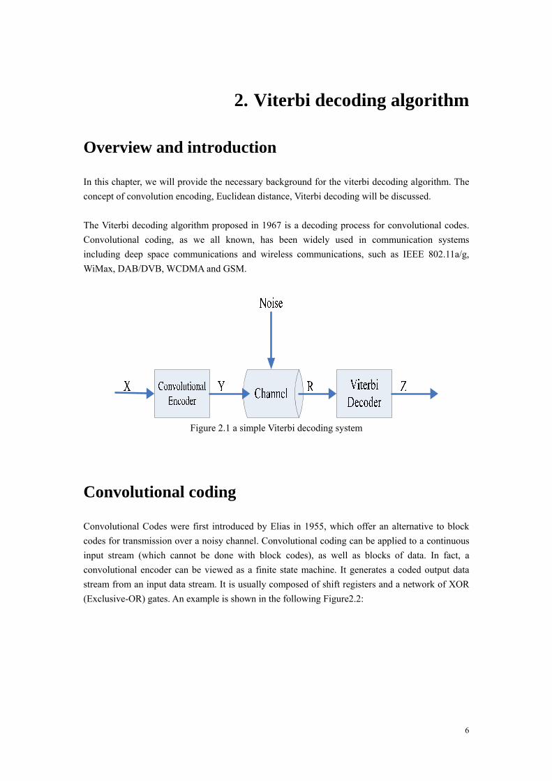
In this chapter, we will provide the necessary background for the viterbi decoding algorithm. The concept of convolution encoding, Euclidean distance, Viterbi decoding will be discussed. The Viterbi decoding algorithm proposed in 1967 is a decoding process for convolutional codes. Convolutional coding, as we all known, has been widely used in communication systems including deep space communications and wireless communications, such as IEEE 802.11a/g, WiMax, DAB/DVB, WCDMA and GSM.
Figure 2.1 a simple Viterbi decoding system
Convolutional coding
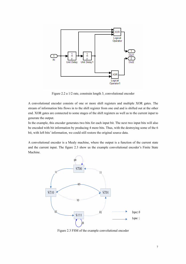
Convolutional Codes were first introduced by Elias in 1955, which offer an alternative to block codes for transmission over a noisy channel. Convolutional coding can be applied to a continuous input stream (which cannot be done with block codes), as well as blocks of data. In fact, a convolutional encoder can be viewed as a finite state machine. It generates a coded output data stream from an input data stream. It is usually composed of shift registers and a network of XOR (Exclusive-OR) gates. An example is shown in the following Figure2.2:
7
Figure 2.2 a 1/2 rate, constrain length 3, convolutional encoder
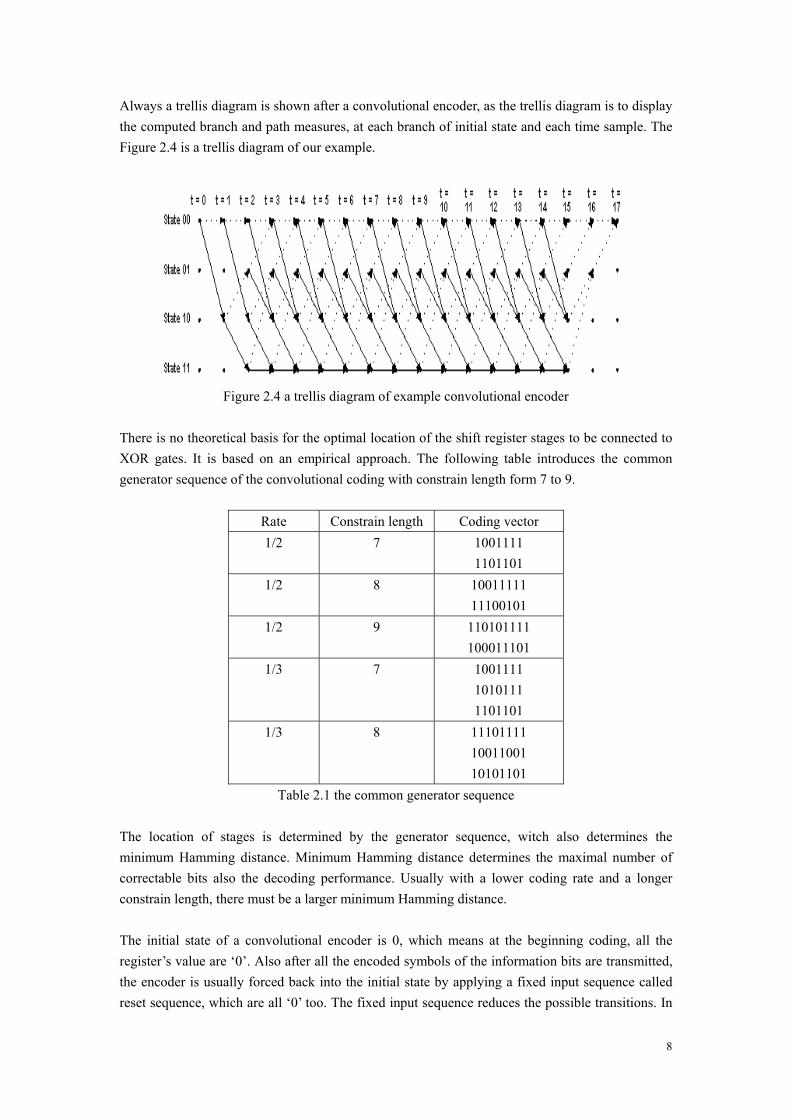
A convolutional encoder consists of one or more shift registers and multiple XOR gates. The stream of information bits flows in to the shift register from one end and is shifted out at the other end. XOR gates are connected to some stages of the shift registers as well as to the current input to generate the output. In the example, this encoder generates two bits for each input bit. The next two input bits will also be encoded with bit information by producing 4 more bits. Thus, with the destroying some of the 6 bit, with left bits’ information, we could still restore the original source data. A convolutional encoder is a Mealy machine, where the output is a function of the current state and the current input. The figure 2.3 show us the example convolutional encoder’s Finite State Machine.
Figure 2.3 FSM of the example convolutional encoder
8
Always a trellis diagram is shown after a convolutional encoder, as the trellis diagram is to display the computed branch and path measures, at each branch of initial state and each time sample. The Figure 2.4 is a trellis diagram of our example.
Figure 2.4 a trellis diagram of example convolutional encoder
There is no theoretical basis for the optimal location of the shift register stages to be connected to XOR gates. It is based on an empirical approach. The following table introduces the common generator sequence of the convolutional coding with constrain length form 7 to 9.
Rate Constrain length Coding vector 1/2 7 1001111
1101101 1/2 8 10011111
11100101 1/2 9 110101111
100011101 1/3 7 1001111
1010111 1101101
1/3 8 11101111 10011001 10101101
Table 2.1 the common generator sequence The location of stages is determined by the generator sequence, witch also determines the minimum Hamming distance. Minimum Hamming distance determines the maximal number of correctable bits also the decoding performance. Usually with a lower coding rate and a longer constrain length, there must be a larger minimum Hamming distance. The initial state of a convolutional encoder is 0, which means at the beginning coding, all the register’s value are ‘0’. Also after all the encoded symbols of the information bits are transmitted, the encoder is usually forced back into the initial state by applying a fixed input sequence called reset sequence, which are all ‘0’ too. The fixed input sequence reduces the possible transitions. In
9
this manner, the trellis shrinks until it reaches the initial state. It should be noted that, there is a unique path for every code word that begins and stops at the initial state.
Euclidean distance
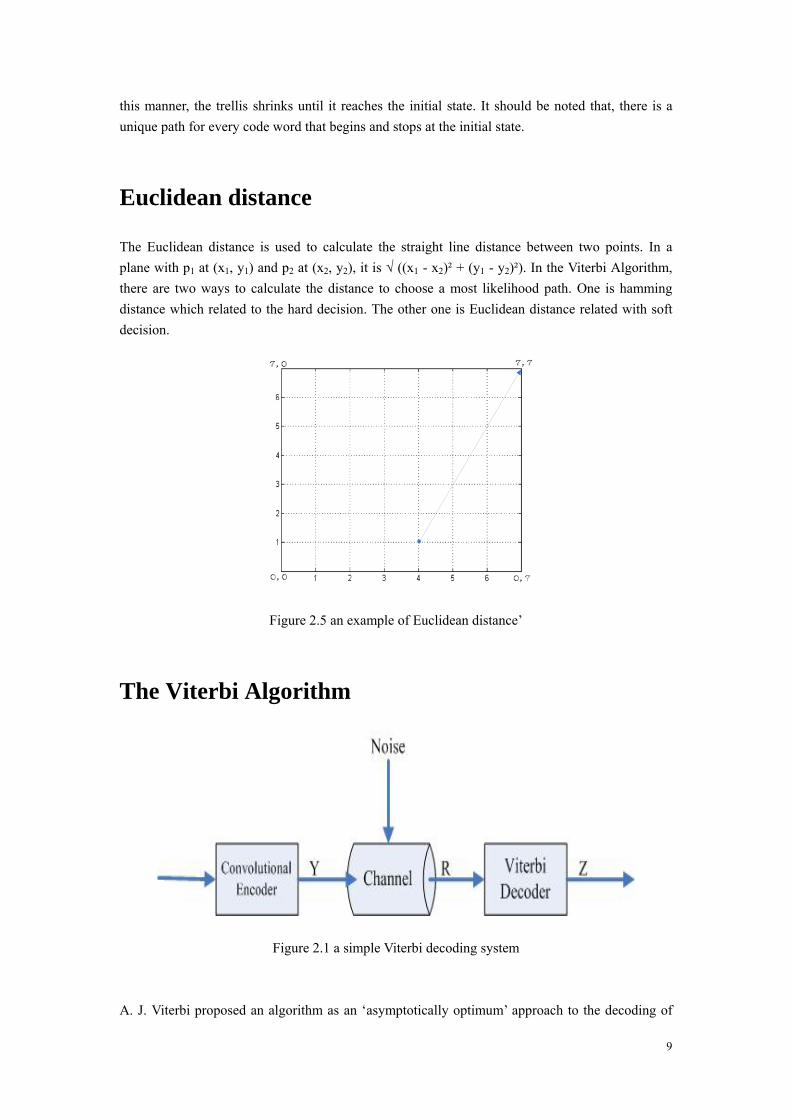
The Euclidean distance is used to calculate the straight line distance between two points. In a plane with p1 at (x1, y1) and p2 at (x2, y2), it is √ ((x1 - x2)² + (y1 - y2)²). In the Viterbi Algorithm, there are two ways to calculate the distance to choose a most likelihood path. One is hamming distance which related to the hard decision. The other one is Euclidean distance related with soft decision.
Figure 2.5 an example of Euclidean distance’
The Viterbi Algorithm
Figure 2.1 a simple Viterbi decoding system A. J. Viterbi proposed an algorithm as an ‘asymptotically optimum’ approach to the decoding of
10
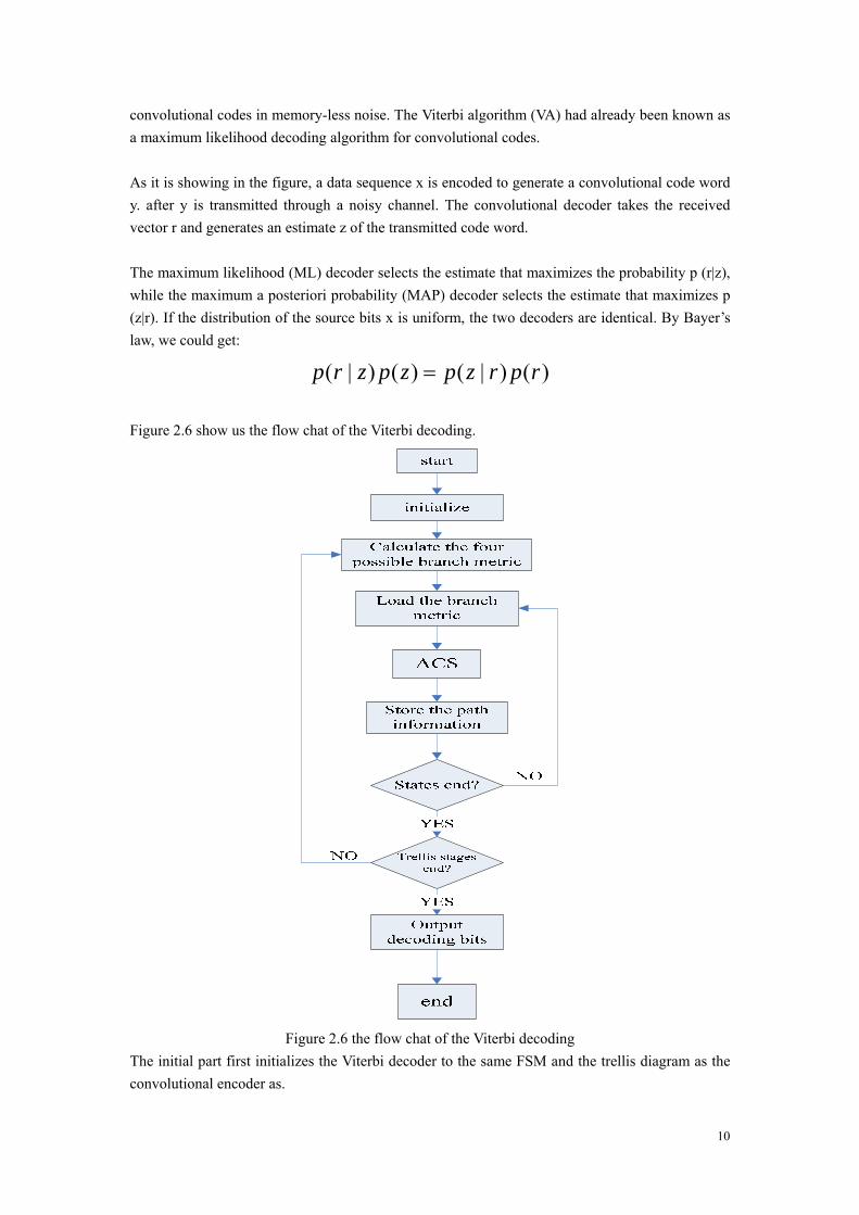
convolutional codes in memory-less noise. The Viterbi algorithm (VA) had already been known as a maximum likelihood decoding algorithm for convolutional codes. As it is showing in the figure, a data sequence x is encoded to generate a convolutional code word y. after y is transmitted through a noisy channel. The convolutional decoder takes the received vector r and generates an estimate z of the transmitted code word. The maximum likelihood (ML) decoder selects the estimate that maximizes the probability p (r|z), while the maximum a posteriori probability (MAP) decoder selects the estimate that maximizes p (z|r). If the distribution of the source bits x is uniform, the two decoders are identical. By Bayer’s law, we could get:
)()|()()|( rprzpzpzrp = Figure 2.6 show us the flow chat of the Viterbi decoding.
Figure 2.6 the flow chat of the Viterbi decoding
The initial part first initializes the Viterbi decoder to the same FSM and the trellis diagram as the convolutional encoder as.

11
Then in each time clock, the decoder computes the four possible branches metric’s Euclidean distance. For each state, ACS block compute the two possible paths Euclidean distance and select a small one. At the same time, ACS block will record the survival state metric. A trellis structure is built along the way, where each state transition is noted with all the relevant information like path metric and the decision bit. When all the data bits have been received, and the trellis has been completed, the last stage of the trellis is used as the starting point for tracing back. The trace-back operation outputs the decoded data, as it traces back along the maximum likelihood path.
12
3. Behavior model of the Viterbi Decoder
System Overview
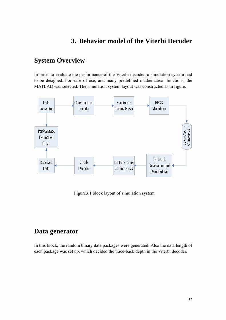
In order to evaluate the performance of the Viterbi decoder, a simulation system had to be designed. For ease of use, and many predefined mathematical functions, the MATLAB was selected. The simulation system layout was constructed as in figure.
Figure3.1 block layout of simulation system
Data generator
In this block, the random binary data packages were generated. Also the data length of each package was set up, which decided the trace-back depth in the Viterbi decoder.
13
Convolutional Encoder
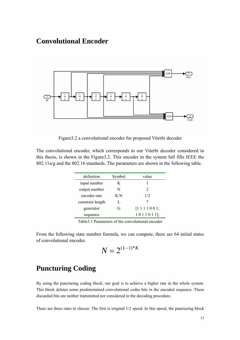
Figure3.2 a convolutional encoder for proposed Viterbi decoder
The convolutional encoder, which corresponds to our Viterbi decoder considered in this thesis, is shown in the Figure3.2. This encoder in the system full fills IEEE the 802.11a/g and the 802.16 standards. The parameters are shown in the following table.
definition Symbol value input number K 1 output number N 2 encoder rate K/N 1/2
constrain length L 7 generator sequence
G [1 1 1 1 0 0 1; 1 0 1 1 0 1 1];
Table3.1 Parameters of the convolutional encoder From the following state number formula, we can compute, there are 64 initial states of convolutional encoder.
KLN *)1(2 −=
Puncturing Coding
By using the puncturing coding block, our goal is to achieve a higher rate in the whole system. This block deletes some predetermined convolutional codes bits in the encoded sequence. These discarded bits are neither transmitted nor considered in the decoding procedure. There are three rates to choose. The first is original 1/2 speed. In this speed, the puncturing block
14
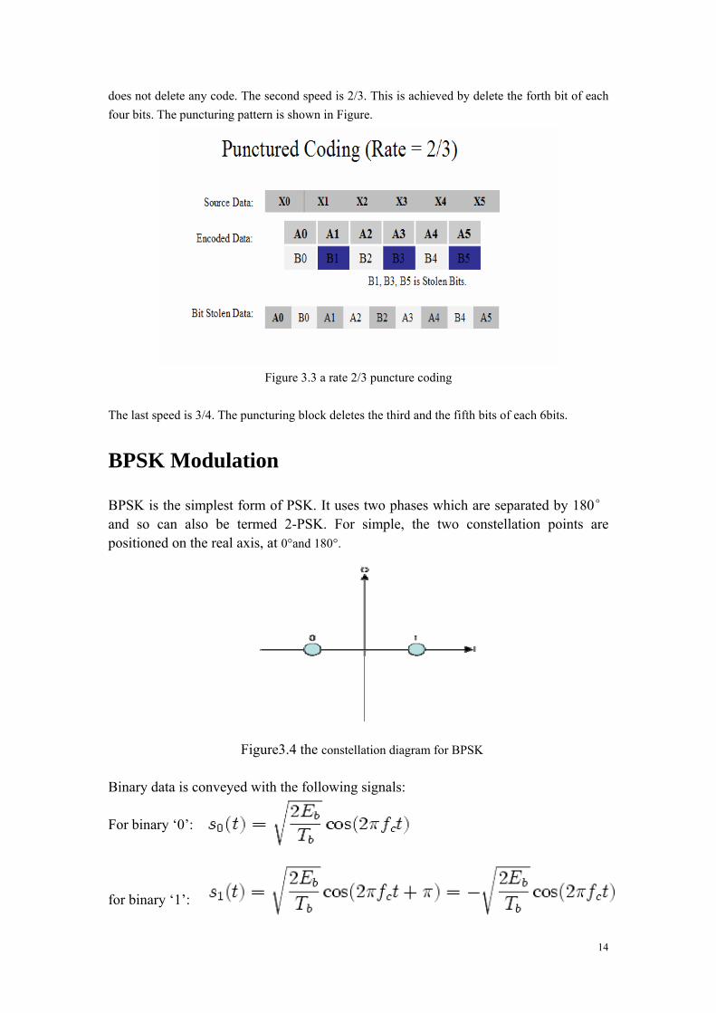
does not delete any code. The second speed is 2/3. This is achieved by delete the forth bit of each four bits. The puncturing pattern is shown in Figure.
Figure 3.3 a rate 2/3 puncture coding
The last speed is 3/4. The puncturing block deletes the third and the fifth bits of each 6bits.
BPSK Modulation
BPSK is the simplest form of PSK. It uses two phases which are separated by 180° and so can also be termed 2-PSK. For simple, the two constellation points are positioned on the real axis, at 0°and 180°.
Figure3.4 the constellation diagram for BPSK Binary data is conveyed with the following signals: For binary ‘0’: for binary ‘1’:
15
AWGN channel
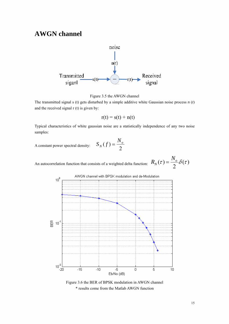
Figure 3.5 the AWGN channel The transmitted signal s (t) gets disturbed by a simple additive white Gaussian noise process n (t) and the received signal r (t) is given by:
r(t) = s(t) + n(t) Typical characteristics of white gaussian noise are a statistically independence of any two noise samples:
A constant power spectral density: 2)( o
NN
fS =
An autocorrelation function that consists of a weighted delta function: )(2
)( τδτ oN
NR =
Figure 3.6 the BER of BPSK modulation in AWGN channel
* results come from the Matlab AWGN function
16
De-modulation
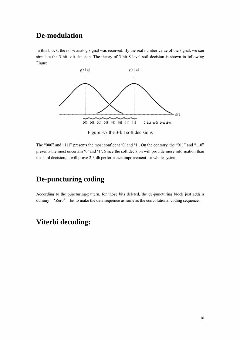
In this block, the noise analog signal was received. By the real number value of the signal, we can simulate the 3 bit soft decision. The theory of 3 bit 8 level soft decision is shown in following Figure.
Figure 3.7 the 3-bit soft decisions
The “000” and “111” presents the most confident ‘0’ and ‘1’. On the contrary, the “011” and “110” presents the most uncertain ‘0’ and ‘1’. Since the soft decision will provide more information than the hard decision, it will prove 2-3 db performance improvement for whole system.
De-puncturing coding
According to the puncturing-pattern, for those bits deleted, the de-puncturing block just adds a dummy ‘Zero’ bit to make the data sequence as same as the convolutional coding sequence.
Viterbi decoding:
17
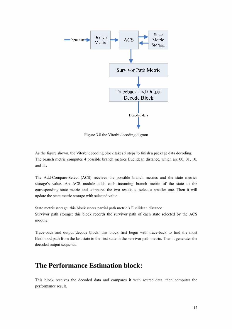
Figure 3.8 the Viterbi decoding digram
As the figure shown, the Viterbi decoding block takes 5 steps to finish a package data decoding. The branch metric computes 4 possible branch metrics Euclidean distance, which are 00, 01, 10, and 11. The Add-Compare-Select (ACS) receives the possible branch metrics and the state metrics storage’s value. An ACS module adds each incoming branch metric of the state to the corresponding state metric and compares the two results to select a smaller one. Then it will update the state metric storage with selected value. State metric storage: this block stores partial path metric’s Euclidean distance. Survivor path storage: this block records the survivor path of each state selected by the ACS module. Trace-back and output decode block: this block first begin with trace-back to find the most likelihood path from the last state to the first state in the survivor path metric. Then it generates the decoded output sequence.
The Performance Estimation block:
This block receives the decoded data and compares it with source data, then computer the performance result.
18
4. RTL model of the Viterbi Decoder
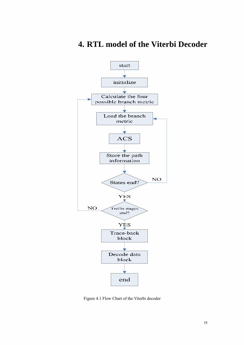
Figure 4.1 Flow Chart of the Viterbi decoder
19
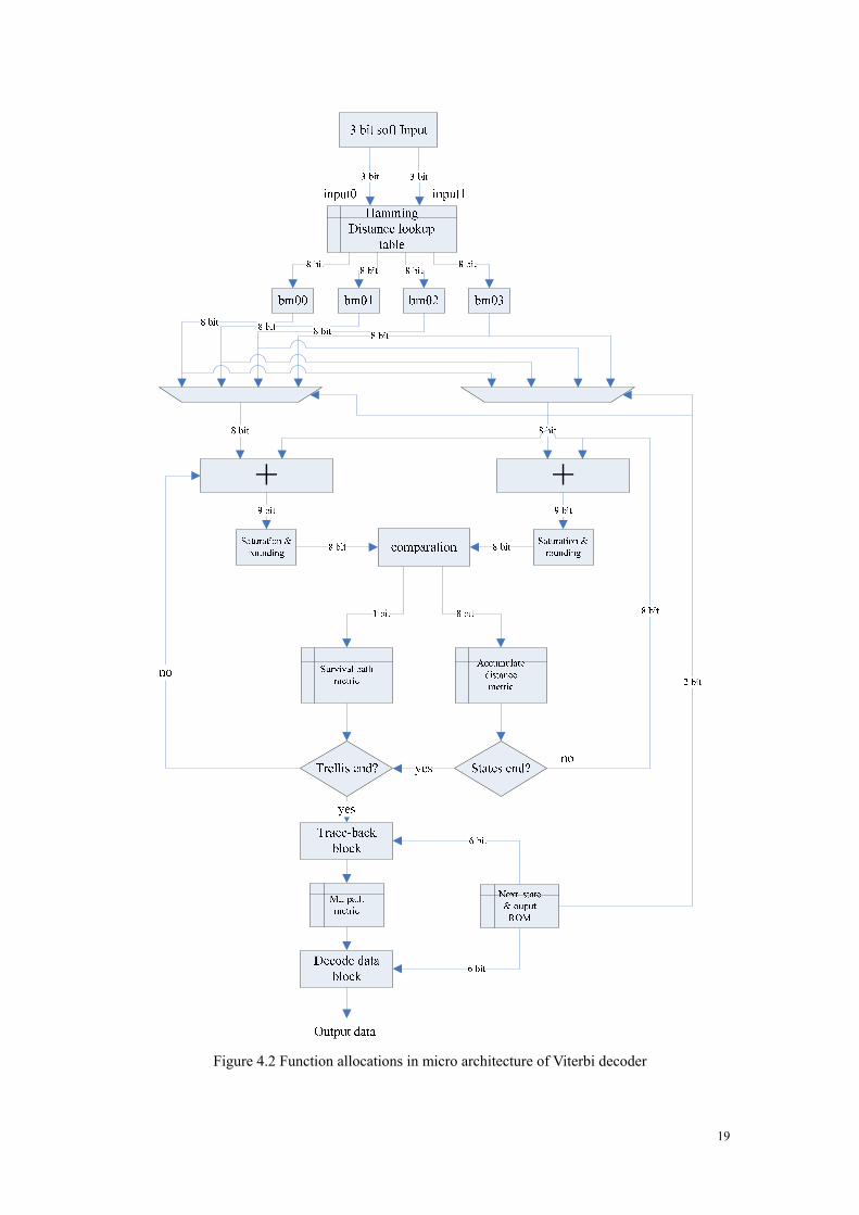
Figure 4.2 Function allocations in micro architecture of Viterbi decoder
20
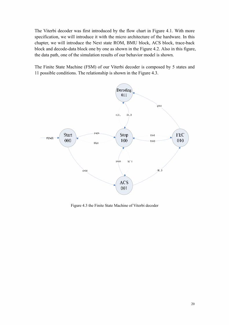
The Viterbi decoder was first introduced by the flow chart in Figure 4.1. With more specification, we will introduce it with the micro architecture of the hardware. In this chapter, we will introduce the Next state ROM, BMU block, ACS block, trace-back block and decode-data block one by one as shown in the Figure 4.2. Also in this figure, the data path, one of the simulation results of our behavior model is shown. The Finite State Machine (FSM) of our Viterbi decoder is composed by 5 states and 11 possible conditions. The relationship is shown in the Figure 4.3.
Figure 4.3 the Finite State Machine of Viterbi decoder
21
The Next state ROM:
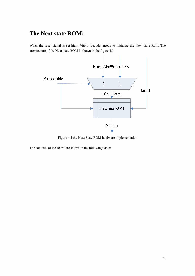
When the reset signal is set high, Viterbi decoder needs to initialize the Next state Rom. The architecture of the Next state ROM is shown in the figure 4.3.
Figure 4.4 the Next State ROM hardware implementation
The contexts of the ROM are shown in the following table:
22
Previous state
Next state and 2output-bit With Input 0
Next state and 2output-bit With Input 1
Previous state
Next state and 2output-bit With Input 0
Next state and 2output-bit With Input 1
000000 00000000 10000011 100000 01000010 11000001 000001 00000011 10000000 100001 01000001 11000010 000010 00000101 10000110 100010 01000111 11000100 000011 00000110 10000101 100011 01000100 11000111 000100 00001000 10001011 100100 01001010 11001001 000101 00001011 10001000 100101 01001001 11001010 000110 00001101 10001110 100110 01001111 11001100 000111 00001110 10001101 100111 01001100 11001111 001000 00010011 10010000 101000 01010001 11010010 001001 00010000 10010011 101001 01010010 11010001 001010 00010110 10010101 101010 01010100 11010111 001011 00010101 10010110 101011 01010111 11010100 001100 00011011 10011000 101100 01011001 11011010 001101 00011000 10011011 101101 01011010 11011001 001110 00011110 10011101 101110 01011100 11011111 001111 00011101 10011110 101111 01011111 11011100 010000 00100011 10100000 110000 01100001 11100010 010001 00100000 10100011 110001 01100010 11100001 010010 00100110 10100101 110010 01100100 11100111 010011 00100101 10100110 110011 01100111 11100100 010100 00101011 10101000 110100 01101001 11101010 010101 00101000 10101011 110101 01101010 11101001 010110 00101110 10101101 110110 01101100 11101111 010111 00101101 10101110 110111 01101111 11101100 011000 00110000 10110011 111000 01110010 11110001 011001 00110011 10110000 111001 01110001 11110010 011010 00110101 10110110 111010 01110111 11110100 011011 00110110 10110101 111011 01110100 11110111 011100 00111000 10111011 111100 01111010 11111001 011101 00111011 10111000 111101 01111001 11111010 011110 00111101 10111110 111110 01111111 11111110 011111 00111110 10111101 111111 01111100 11111111
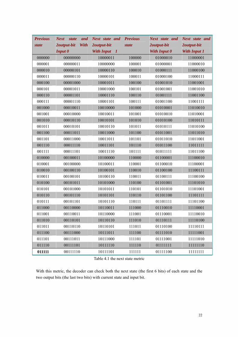
Table 4.1 the next state metric
With this metric, the decoder can check both the next state (the first 6 bits) of each state and the two output bits (the last two bits) with current state and input bit.
23
The BMU block:
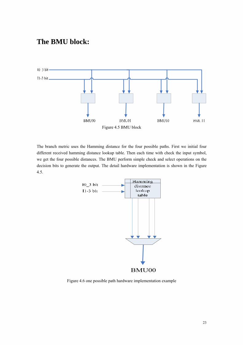
Figure 4.5 BMU block
The branch metric uses the Hamming distance for the four possible paths. First we initial four different received hamming distance lookup table. Then each time with check the input symbol, we get the four possible distances. The BMU perform simple check and select operations on the decision bits to generate the output. The detail hardware implementation is shown in the Figure 4.5.
Figure 4.6 one possible path hardware implementation example

24
The ACS block
When the 4 possible input distance is ready, the ACS block’ butterfly module adds the results and the related distance value stored in the state metric storage to get the each two paths for the 64 initial states. The butterfly module is shown in the next figure. Since, each butterfly computes 4 possible paths and selects the two smaller distance paths form. We have totally 32 butterflies.
Figure 4.7 the butterfly module
For each nod (state), the ACS module selects a smaller one as the survival path and stores them to the accumulated state metric storage block and the survivor path metric. Following Figure is the ACS module.
8 bit full adder
BMU00
8 bit full adder
BMU11
Survivor PM 0 1
accumulated state metric storage
FEC Figure 4.8 the ACS Module
25
When trellis diagram is reached its finial state, the survivor path metric is been set up. In this metric, it use one bit to record all the survival states from which one of the previous state (0 is from higher path with 1 from lower path.).
The Trace-back block
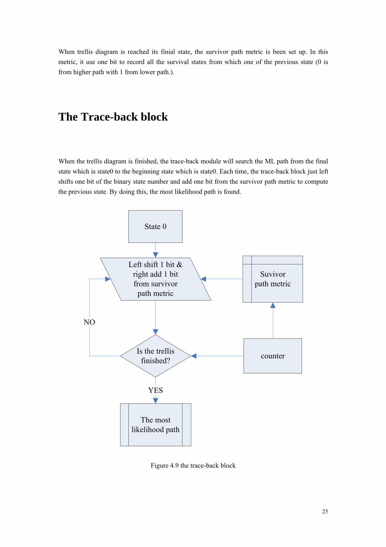
When the trellis diagram is finished, the trace-back module will search the ML path from the final state which is state0 to the beginning state which is state0. Each time, the trace-back block just left shifts one bit of the binary state number and add one bit from the survivor path metric to compute the previous state. By doing this, the most likelihood path is found.
Suvivor path metric
Left shift 1 bit & right add 1 bit from survivor
path metric
The most likelihood path
counter
State 0
Is the trellis finished?
NO
YES
Figure 4.9 the trace-back block
26
The decoding block
Figure 4.10 the decode data block
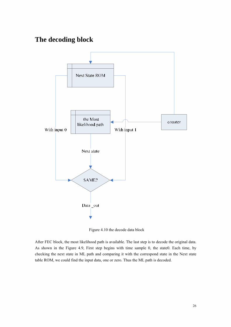
After FEC block, the most likelihood path is available. The last step is to decode the original data. As shown in the Figure 4.9, First step begins with time sample 0, the state0. Each time, by checking the next state in ML path and comparing it with the correspond state in the Next state table ROM, we could find the input data, one or zero. Thus the ML path is decoded.
27
5. Results
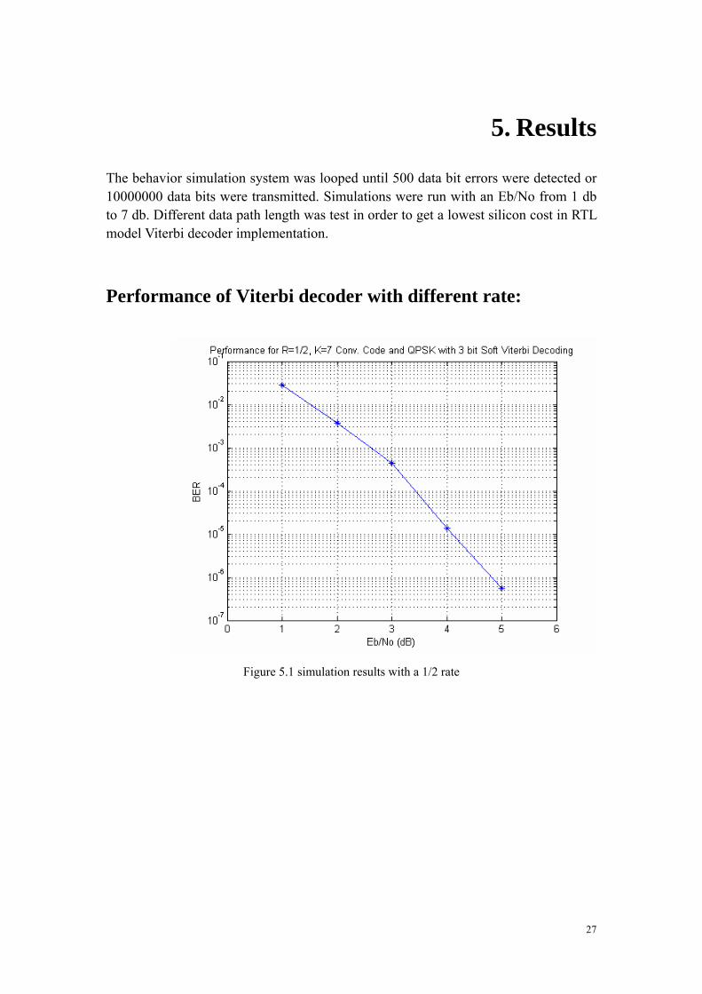
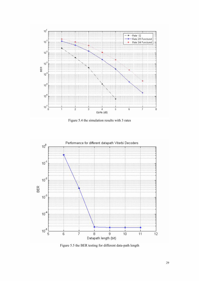
The behavior simulation system was looped until 500 data bit errors were detected or 10000000 data bits were transmitted. Simulations were run with an Eb/No from 1 db to 7 db. Different data path length was test in order to get a lowest silicon cost in RTL model Viterbi decoder implementation.
Performance of Viterbi decoder with different rate:
Figure 5.1 simulation results with a 1/2 rate
28
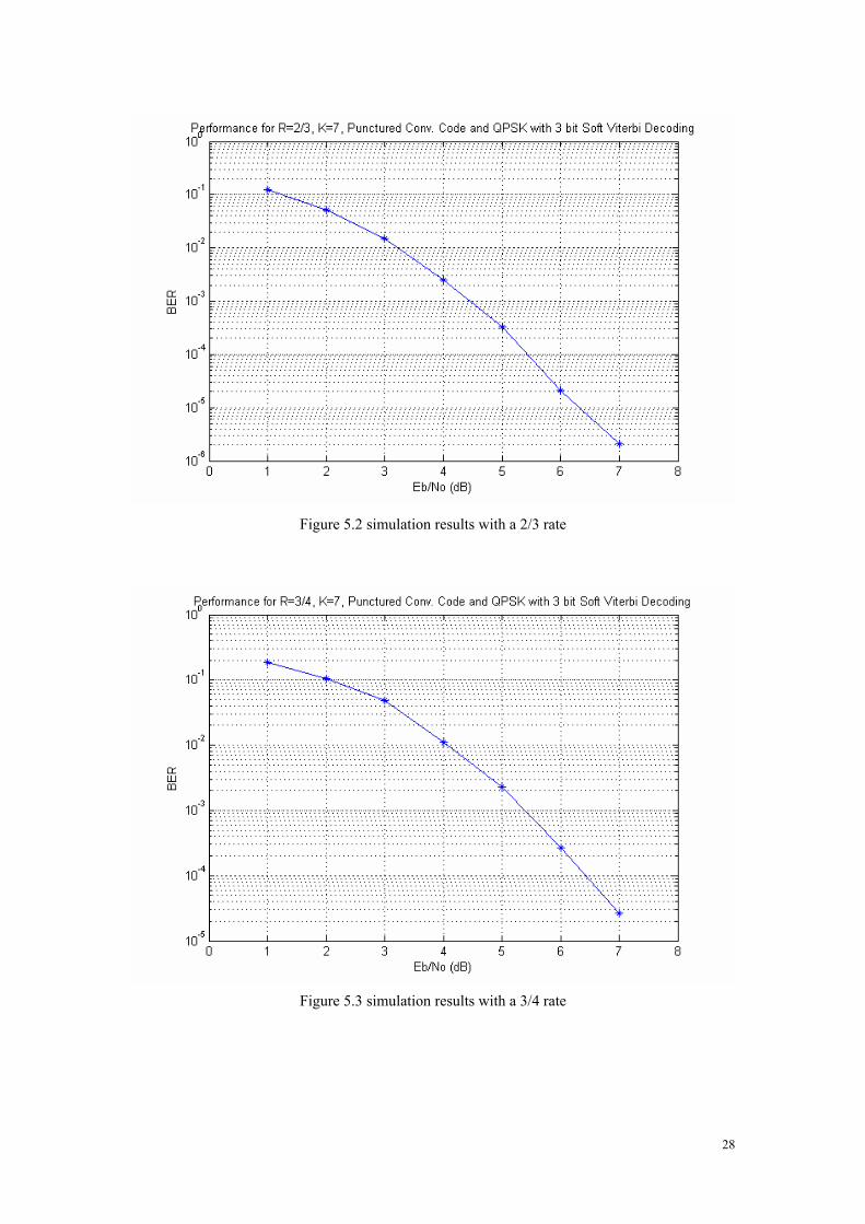
Figure 5.2 simulation results with a 2/3 rate
Figure 5.3 simulation results with a 3/4 rate
29
Figure 5.4 the simulation results with 3 rates
Figure 5.5 the BER testing for different data-path length
30
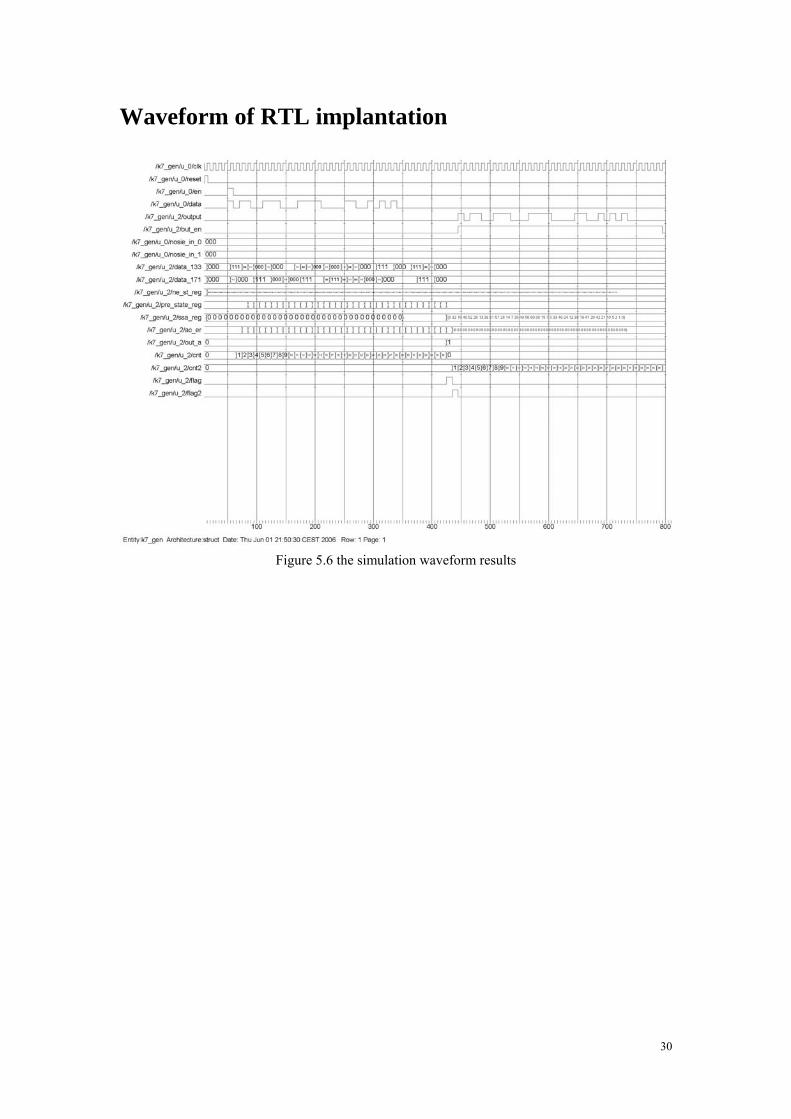
Waveform of RTL implantation
Figure 5.6 the simulation waveform results

31
6. Discussion
By building the convolutional encoder and Viterbi decoder in the behavior model, the MATLAB simulation results give us a light on its performance and how to implement it in a RTL system. From the results, we find the Viterbi decoding algorithm is mature error correct system, which will give us a BER at 8.6E-007 at 5db on an AWGN channel with BPSK modulation. By puncturing, for rate 2/3, we will pay around a 2db cost. For rate 3/4, we will pay for a 3 db cost during the transmission.

32
7. Future work
For the time issue, we do not implement a higher performance Viterbi decoder with such as pipelining or interleaving. So in the future, with Pipeline or interleave the ACS and the trace-back and output decode block, we can make it better. Another trend is to implement a Viterbi decoder in the Turbo code algorithm. With different require specification, there must be a modify in the original design.
33
8. References
[1] Chip Fleming: A Tutorial on Convolutional Coding with Viterbi Decoding; Spectrum Application; Jun, 2003; [2] Dake Liu: Design of Embedded DSP processors; Computer Engineering Division of Electrical Engineering Department, Linköping University; 2004 [3] Stephen B. Wicker: Error Control Systems for Digital Communication and Storage; Prentice Hall; (1995) [4] John G. Proakis, Masoud Salehi; Contemporary communication systems using MATLAB; Brooks; 2000 [5] Rodger E. Ziemer, Roger L. Peterson: Introduction to digital communication; Prentice-Hall International (UK), cop. 2001 [6] Samirkumar Ranpara: On a Viterbi Decoder design for low power dissipation; Virginia Polytechnic Institute and State University; April, 1999; [7] Simon Haykin and Michael Moher: Modern wireless communications; Pearson Prentice Hall, 2005 [8] Simon Haykin; Digital communications; Wiley, cop. 1988 [9] Stephen J. Chapman: MATLAB programming for engineers; Thomson, 2004
34
9. Appendix
Matlab files
data_gen.m function [data] = data_gen(l); % the data generator generates the binary data source with length l temp=rand(1,l); for x= 1:l if(temp(x)<0.5) data(x)=0; else data(x)=1; end end
cnv_encd.m function output=cnv_encd(g,k0,input) % the convolutional encoder % g is the generator matrix of the convolutional code % k0 is the number of bits entering the encoder at each clock cycle. % Check to see if extra zero-padding is necessary. if rem(length(input),k0) > 0 input=[input,zeros(size(1:k0-rem(length(input),k0)))]; end n=length(input)/k0; % Check the size of matrix g. if rem(size(g,2),k0) > 0 error('Error, g is not of the right size.') end % Determine l and n0. l=size(g,2)/k0; n0=size(g,1); % add extra zeros u=[zeros(size(1:(l-1)*k0)),input,zeros(size(1:(l-1)*k0))];
35
u1=u(l*k0:-1:1); for i=1:n+l-2 u1=[u1,u((i+l)*k0:-1:i*k0+1)]; end uu=reshape(u1,l*k0,n+l-1); % Determine the output output=reshape(rem(g*uu,2),1,n0*(l+n-1));
puncture.m function [data_pun] = puncture(data_conv, rate); % the puncturing block, data_conv is the binary data after puncturing % there are 3 kind of rates which is selected by the rate p1 = length(data_conv); if rate == 1 % rate 1/2 data_pun = data_conv; elseif rate == 2 % rate 2/3 if rem(p1, 4) == 0 p2 = p1/4; for i = 1: p2 data_pun(1 + (i-1)*3) = data_conv(1 + (i-1)*4); data_pun(2 + (i-1)*3) = data_conv(2 + (i-1)*4); data_pun(3 + (i-1)*3) = data_conv(3 + (i-1)*4); end else p4 = (p1 - rem(p1, 4))/4; p5 = rem(p1, 4); for i = 1: p4 data_pun(1 + (i-1)*3) = data_conv(1 + (i-1)*4); data_pun(2 + (i-1)*3) = data_conv(2 + (i-1)*4); data_pun(3 + (i-1)*3) = data_conv(3 + (i-1)*4); end for i = 1 : p5 data_pun(3*p4 + i)= data_conv(p1 -p5 +i); end end elseif rate == 3 % rate 3/4 if rem(p1, 6) == 0
36
p3 = p1/6; for i = 1: p3 data_pun(1 + (i-1)*4) = data_conv(1 + (i-1)*6); data_pun(2 + (i-1)*4) = data_conv(2 + (i-1)*6); data_pun(3 + (i-1)*4) = data_conv(3 + (i-1)*6); data_pun(4 + (i-1)*4) = data_conv(6 + (i-1)*6); end else p4 = (p1 - rem(p1, 6))/6; p5 = rem(p1, 6); for i = 1: p4 data_pun(1 + (i-1)*4) = data_conv(1 + (i-1)*6); data_pun(2 + (i-1)*4) = data_conv(2 + (i-1)*6); data_pun(3 + (i-1)*4) = data_conv(3 + (i-1)*6); data_pun(4 + (i-1)*4) = data_conv(6 + (i-1)*6); end for i = 1 : p5 data_pun(4*p4 + i)= data_conv(p1 - p5 + i); end end else error('The setup of rate is out of range!!!') end
awgn_test.m % setup e = 0; l = 50000; snr = 0; % Data generator temp=rand(1,l); for a= 1:l if(temp(a)<0.5) data(a)=0; else data(a)=1; end end % bpsk modulation for b = 1 : l
37
if data(b) == 0 temp1(b) = -1; else temp1(b) = 1; end end % AWGN channel temp2 = awgn(temp1, snr); for c= 1 : l if temp2(c) <= 0 data_dec(c) = 0 ; else data_dec(c) = 1; end end % BER caculation for m= 1:l if (data(m) ~=data_dec(m)), e = e + 1; end end BER = e/l;
bpsk_awgn.m function data_dec = bpsk_awgn(data_pun, hard_soft, snr) %bpsk modulation, awgn and 3 bit soft decision block %data_pun is the data after puncturing l = length(data_pun); if hard_soft == 0 %hard decision for i = 1 : l if data_pun(i) == 0 temp1(i) = -1; else temp1(i) = 1; end end temp2 = awgn(temp1, snr, 0, 1234); for i = 1 : l
38
if temp2(i) <= 0 data_dec(i) = 0 ; else data_dec(i) = 1; end end elseif hard_soft == 1 % 3 bit soft decision for i = 1 : l if data_pun(i) == 0 temp1(i) = -1; else temp1(i) = 1; end end temp2 = awgn(temp1, snr, 0); for i = 1 : l if temp2(i) <= -0.8571 data_dec(i) = 0; elseif temp2(i) <= -0.5714 data_dec(i) = 1; elseif temp2(i) <= -0.2857 data_dec(i) = 2; elseif temp2(i) <= 0 data_dec(i) = 3; elseif temp2(i) <= 0.2857 data_dec(i) = 4; elseif temp2(i) <= 0.5714 data_dec(i) = 5; elseif temp2(i) <= 0.8571 data_dec(i) = 6; elseif temp2(i) > 0.8571 data_dec(i) = 7; end end end
insert_zero.m function [data_insert_zero] = insert_zero (data_soft_de, rate, hard_soft,
fl);
39
% check the sizes if hard_soft == 1 p1 = length(data_soft_de); if rate == 1 data_insert_zero = data_soft_de; elseif rate == 2 if rem(p1, 3) == 0 p2 = p1/3; for i = 1: p2 data_insert_zero(1 + (i-1)*4) = data_soft_de(1 + (i-1)*3); data_insert_zero(2 + (i-1)*4) = data_soft_de(2 + (i-1)*3); data_insert_zero(3 + (i-1)*4) = data_soft_de(3 + (i-1)*3); data_insert_zero(4 + (i-1)*4) = 3; end else p3 = rem(p1, 3); p2 = (p1 - p3)/3; for i = 1: p2 data_insert_zero(1 + (i-1)*4) = data_soft_de(1 + (i-1)*3); data_insert_zero(2 + (i-1)*4) = data_soft_de(2 + (i-1)*3); data_insert_zero(3 + (i-1)*4) = data_soft_de(3 + (i-1)*3); data_insert_zero(4 + (i-1)*4) = 3; end for i= 1: p3 data_insert_zero(4*p2 + i) = data_soft_de(3*p2 + i); end end elseif rate == 3 if rem(p1, 4)~= 0 p3 = rem(p1, 4); p2 = (p1 - p3)/4; for i = 1: p2 data_insert_zero(1 + (i-1)*6) = data_soft_de(1 + (i-1)*4); data_insert_zero(2 + (i-1)*6) = data_soft_de(2 + (i-1)*4); data_insert_zero(3 + (i-1)*6) = 3; data_insert_zero(4 + (i-1)*6) = data_soft_de(3 + (i-1)*4); data_insert_zero(5 + (i-1)*6) = 3; data_insert_zero(6 + (i-1)*6) = data_soft_de(4 + (i-1)*4); end for i= 1: p3 data_insert_zero(6*p2 + i) = data_soft_de(4*p2 + i);
40
end elseif rem(p1, 4) == 0 & fl == 0 p2 = p1/4; for i = 1: p2 data_insert_zero(1 + (i-1)*6) = data_soft_de(1 + (i-1)*4); data_insert_zero(2 + (i-1)*6) = data_soft_de(2 + (i-1)*4); data_insert_zero(3 + (i-1)*6) = 3; data_insert_zero(4 + (i-1)*6) = data_soft_de(3 + (i-1)*4) ; data_insert_zero(5 + (i-1)*6) = 3; data_insert_zero(6 + (i-1)*6) = data_soft_de(4 + (i-1)*4); end elseif rem(p1, 4) == 0 & fl == 1 p2 = p1/4; for i = 1: (p2-1) data_insert_zero(1 + (i-1)*6) = data_soft_de(1 + (i-1)*4); data_insert_zero(2 + (i-1)*6) = data_soft_de(2 + (i-1)*4); data_insert_zero(3 + (i-1)*6) = 3; data_insert_zero(4 + (i-1)*6) = data_soft_de(3 + (i-1)*4) ; data_insert_zero(5 + (i-1)*6) = 3; data_insert_zero(6 + (i-1)*6) = data_soft_de(4 + (i-1)*4); end data_insert_zero((p2-1)*6+1) = data_soft_de((p2-1)*4+1); data_insert_zero((p2-1)*6+2) = data_soft_de((p2-1)*4+2); data_insert_zero((p2-1)*6+3) = data_soft_de((p2-1)*4+3); data_insert_zero((p2-1)*6+4) = data_soft_de((p2-1)*4+4); end else error('The setup of rate is out of range!!!') end elseif hard_soft == 0 p1 = length(data_soft_de); if rate == 1 data_insert_zero = data_soft_de; elseif rate == 2 if rem(p1, 3) == 0 p2 = p1/3; for i = 1: p2 data_insert_zero(1 + (i-1)*4) = data_soft_de(1 + (i-1)*3); data_insert_zero(2 + (i-1)*4) = data_soft_de(2 + (i-1)*3); data_insert_zero(3 + (i-1)*4) = data_soft_de(3 + (i-1)*3);
41
data_insert_zero(4 + (i-1)*4) = 0; end else p3 = rem(p1, 3); p2 = (p1 - p3)/3; for i = 1: p2 data_insert_zero(1 + (i-1)*4) = data_soft_de(1 + (i-1)*3); data_insert_zero(2 + (i-1)*4) = data_soft_de(2 + (i-1)*3); data_insert_zero(3 + (i-1)*4) = data_soft_de(3 + (i-1)*3); data_insert_zero(4 + (i-1)*4) = 0; end for i= 1: p3 data_insert_zero(4*p2 + i) = data_soft_de(3*p2 + i); end end elseif rate == 3 if rem(p1, 4)~= 0 p3 = rem(p1, 4); p2 = (p1 - p3)/4; for i = 1: p2 data_insert_zero(1 + (i-1)*6) = data_soft_de(1 + (i-1)*4); data_insert_zero(2 + (i-1)*6) = data_soft_de(2 + (i-1)*4); data_insert_zero(3 + (i-1)*6) = 0; data_insert_zero(4 + (i-1)*6) = data_soft_de(3 + (i-1)*4); data_insert_zero(5 + (i-1)*6) = 0; data_insert_zero(6 + (i-1)*6) = data_soft_de(4 + (i-1)*4); end for i= 1: p3 data_insert_zero(6*p2 + i) = data_soft_de(4*p2 + i); end elseif rem(p1, 4) == 0 & fl == 0 p2 = p1/4; for i = 1: p2 data_insert_zero(1 + (i-1)*6) = data_soft_de(1 + (i-1)*4); data_insert_zero(2 + (i-1)*6) = data_soft_de(2 + (i-1)*4); data_insert_zero(3 + (i-1)*6) = 0; data_insert_zero(4 + (i-1)*6) = data_soft_de(3 + (i-1)*4) ; data_insert_zero(5 + (i-1)*6) = 0; data_insert_zero(6 + (i-1)*6) = data_soft_de(4 + (i-1)*4); end elseif rem(p1, 4) == 0 & fl ~= 0 p2 = p1/4;
42
for i = 1: p2-2 data_insert_zero(1 + (i-1)*6) = data_soft_de(1 + (i-1)*4); data_insert_zero(2 + (i-1)*6) = data_soft_de(2 + (i-1)*4); data_insert_zero(3 + (i-1)*6) = 0; data_insert_zero(4 + (i-1)*6) = data_soft_de(3 + (i-1)*4) ; data_insert_zero(5 + (i-1)*6) = 0; data_insert_zero(6 + (i-1)*6) = data_soft_de(4 + (i-1)*4); end data_insert_zero((p2-2)*6+1) = data_soft_de((p2-1)*4+1); data_insert_zero((p2-2)*6+2) = data_soft_de((p2-1)*4+2); data_insert_zero((p2-2)*6+3) = data_soft_de((p2-1)*4+3); data_insert_zero((p2-2)*6+4) = data_soft_de((p2-1)*4+4); end else error('The setup of rate is out of range!!!') end end
flag.m function [pun]= flag(data_soft_de, rate); % generate the flag for Viterbi decoder dealing with the dummy zeros l = length(data_soft_de); if rate == 1 for i=1:l pun(l) = 0; end elseif rate == 2 for i=1:l if rem (i, 4) == 0 pun(i)=1; else pun(i)=0; end end elseif rate == 3 t1 = (l-rem(l,6))/6; for i=0:t1-1 pun(6*(i)+1)=0; pun(6*(i)+2)=0; pun(6*(i)+3)=1;
43
pun(6*(i)+4)=0; pun(6*(i)+5)=1; pun(6*(i)+6)=0; end for j =( l - rem(l,6) ):l pun(j)=0; end end
Viterbi.m function [decoder_output]=viterbi(G,k,channel_output,data_pun) % The Viterbi decoder for convolutional codes n=size(G,1); % check the sizes if rem(size(G,2),k) ~=0 error('Size of G and k do not agree') end if rem(size(channel_output,2),n) ~=0 error('channel output not of the right size') end L=size(G,2)/k; number_of_states=2^((L-1)*k); % Generate state transition matrix, output matrix, and input matrix. for j=0:number_of_states-1 for l=0:2^k-1 [next_state,memory_contents]=nxt_stat(j,l,L,k); input(j+1,next_state+1)=l; branch_output=rem(memory_contents*G',2); nextstate(j+1,l+1)=next_state; output(j+1,l+1)=bin2deci(branch_output); end end state_metric=zeros(number_of_states,2); depth_of_trellis=length(channel_output)/n; channel_output_matrix=reshape(channel_output,n,depth_of_trellis); survivor_state=zeros(number_of_states,depth_of_trellis+1); flag_output=reshape(flag_data,n,depth_of_trellis); % Start decoding of non-tail channel outputs.
44
for i=1:depth_of_trellis-L+1 flag=zeros(1,number_of_states); if i <= L step=2^((L-i)*k); else step=1; end for j=0:step:number_of_states-1 for l=0:2^k-1 branch_metric=0; binary_output=deci2bin(output(j+1,l+1),n); for ll=1:n if flag_output(ll,i)==0
branch_metric=branch_metric+metric1(channel_output_matrix(ll,i),binar
y_output(ll)); else branch_metric= branch_metric; end end if((state_metric(nextstate(j+1,l+1)+1,2) >
state_metric(j+1,1)+branch_metric) | flag(nextstate(j+1,l+1)+1)==0) % state_metric(nextstate(j+1,l+1)+1,2) =
state_metric(j+1,1)+branch_metric; a = state_metric(j+1,1)+branch_metric; if a >511 a = 511 ; end state_metric(nextstate(j+1,l+1)+1,2) = a; survivor_state(nextstate(j+1,l+1)+1,i+1)=j; flag(nextstate(j+1,l+1)+1)=1; end end end state_metric=state_metric(:,2:-1:1); end % Start decoding of the tail channel-outputs. for i=depth_of_trellis-L+2:depth_of_trellis flag=zeros(1,number_of_states);
45
last_stop=number_of_states/(2^((i-depth_of_trellis+L-2)*k)); for j=0:last_stop-1 branch_metric=0; binary_output=deci2bin(output(j+1,1),n); for ll=1:n if flag_output(ll,i)==0
branch_metric=branch_metric+metric1(channel_output_matrix(ll,i),binar
y_output(ll)); else branch_metric= branch_metric; end end if((state_metric(nextstate(j+1,1)+1,2) > state_metric(j+1,1)... +branch_metric) | flag(nextstate(j+1,1)+1)==0) %state_metric(nextstate(j+1,1)+1,2)=
state_metric(j+1,1)+branch_metric; a = state_metric(j+1,1)+branch_metric; if a > 511 a = 511; end state_metric(nextstate(j+1,1)+1,2) = a; survivor_state(nextstate(j+1,1)+1,i+1)=j; flag(nextstate(j+1,1)+1)=1; end end state_metric=state_metric(:,2:-1:1); end % Generate the decoder output from the optimal path. state_sequence=zeros(1,depth_of_trellis+1); state_sequence(1,depth_of_trellis)=survivor_state(1,depth_of_trellis+
1); for i=1:depth_of_trellis
state_sequence(1,depth_of_trellis-i+1)=survivor_state((state_sequence
(1,depth_of_trellis+2-i)... +1),depth_of_trellis-i+2); end decodeder_output_matrix=zeros(k,depth_of_trellis-L+1); for i=1:depth_of_trellis-L+1
dec_output_deci=input(state_sequence(1,i)+1,state_sequence(1,i+1)+1);
46
dec_output_bin=deci2bin(dec_output_deci,k); decoder_output_matrix(:,i)=dec_output_bin(k:-1:1)'; end decoder_output=reshape(decoder_output_matrix,1,k*(depth_of_trellis-L+
1)); cumulated_metric=state_metric(1,1);
bin2deci.m % binary to decimal
function y=bin2deci(x) l=length(x); y=(l-1:-1:0); y=2.^y; y=x*y';
deci2bin.m % decimal to binary function y=deci2bin(x,l) y = zeros(1,l); i = 1; while x>=0 & i<=l y(i)=rem(x,2); x=(x-y(i))/2; i=i+1; end y=y(l:-1:1);
metric.m function distance=metric(x,y) % calculate the Hamming distance if y == 1 distance= (7 - x);
else distance=(x);
end
47
top_level_viterbi_decoding.m % top level of the Viterbi decoder close all; clear all; clc % MATLAB script for viterbi simulation % the viterbi decoder's constrain lenth is 7, with hard decision. %setup the inistal state n = 0; % the total number of testing data package l = 29; % the input data length e = 0; % errors found in the simulation snr = 1; % snr ratio in db. g = [1 1 1 1 0 0 1; 1 0 1 1 0 1 1]; sequence generator k = 1; % input bit number hard_soft = 1; % 0 hard decision, 1 soft decision rate = 3; % coding rate with punturing, 1 with rate 1/2, 2 with rate 2/3,
3 with rate 3/4, %check the data source length if rem(l,6)~= 0 fl = 1; else fl = 0; end %convolution coding part while n < 10000 n= n + 1; %data generator: data = data_gen(l); % convolutional encoder data_conv = cnv_encd(g, k, data); % puncturing block data_pun = puncture(data_conv, rate); % BPSK modulation and AWGN channel data_dec = bpsk_awgn(data_pun, hard_soft, snr); % depuncturing block
48
data_insert_zero = insert_zero(data_dec, rate, hard_soft, fl); flag_pun = flag(data_insert_zero, rate); % Viterbi decoder data_decoded = viterbi(g,k,data_insert_zero,flag_pun); % checking the decoded data with data source for m= 1:l if (data(m) ~=data_decoded(m)), e = e + 1; end end end % caculate the BER p = e/(n*l);
49
vhdl files
sin_gen.vhdl
--generate the necessary signals for the Viterbi decoder test bench
LIBRARY ieee;
USE ieee.std_logic_1164.all;
USE ieee.std_logic_arith.all;
USE ieee.std_logic_unsigned.all;
ENTITY gen IS
PORT(
clk, reset : OUT std_logic;
en : OUT std_logic;
data : OUT std_logic;
nosie_in_0, nosie_in_1 : OUT std_logic_vector(2 downto 0)
);
-- Declarations
END gen ;
--
ARCHITECTURE sig OF gen IS
constant period : time := 10 ns;
signal Clk_gen : std_logic := '0';
BEGIN
process(Clk_gen)
begin
Clk_gen <= not Clk_gen after period/2;
end process;
clk <= Clk_gen;
reset <= '0',
'1' after 11 ns,
'0' after 16 ns;
data <= '0',
'0' after 11 ns,
'1' after 50 ns,
50
'0' after 60 ns,
'1' after 70 ns,
'1' after 80 ns,
'0' after 90 ns,
'0' after 100 ns,
'1' after 110 ns,
'1' after 120 ns,
'1' after 130 ns,
'0' after 140 ns,
'0' after 150 ns,
'0' after 160 ns,
'1' after 170 ns,
'1' after 180 ns,
'1' after 190 ns,
'1' after 200 ns,
'0' after 210 ns,
'0' after 220 ns,
'0' after 230 ns,
'0' after 240 ns,
'1' after 250 ns,
'1' after 260 ns,
'0' after 270 ns,
'0' after 280 ns,
'1' after 290 ns,
'0' after 300 ns,
'1' after 310 ns,
'0' after 320 ns,
'1' after 330 ns,
'0' after 340 ns,
'0' after 350 ns,
'0' after 360 ns,
'0' after 370 ns,
'0' after 380 ns,
'0' after 390 ns;
en <= '0',
'0' after 11 ns,
'1' after 50 ns,
'0' after 60 ns;
nosie_in_0 <= "000";
nosie_in_1 <= "000";
END ARCHITECTURE sig;
51
Conv_Encoder.vhdl
-- the convolutional encoder
LIBRARY ieee;
USE ieee.std_logic_1164.all;
USE ieee.std_logic_arith.all;
USE ieee.std_logic_unsigned.all;
ENTITY enc IS
PORT(
clk : IN std_logic;
reset : IN std_logic;
en, data : IN std_logic;
enable : OUT std_logic;
data_en : OUT std_logic_vector (1 DOWNTO 0)
);
-- Declarations
END enc ;
--
ARCHITECTURE k7 OF enc IS
signal ff : std_logic_vector( 6 downto 0 );
BEGIN
process(clk, reset)
begin
if clk'event and clk ='1' then
if reset = '1' then
ff <= "0000000";
else
ff <= ff(5 downto 0) & data ;
if en = '1' then
enable <= '1';
else enable <= '0';
end if;
end if;
end if;
end process;
52
data_en(0) <= ff(0) xor ff(2) xor ff(3) xor ff(5) xor ff(6); -- 133
data_en(1) <= ff(0) xor ff(1) xor ff(2) xor ff(3) xor ff(6); -- 171
END ARCHITECTURE k7;
Noise.vhdl
-- add noise to the encoded data
LIBRARY ieee;
USE ieee.std_logic_1164.all;
USE ieee.std_logic_arith.all;
USE ieee.std_logic_unsigned.all;
ENTITY k7_noise IS
END ENTITY k7_noise ;
ARCHITECTURE k7 OF k7_noise IS
BEGIN
process(in_data)
variable in_data_0 : std_logic_vector(2 downto 0);
variable in_data_1 : std_logic_vector(2 downto 0);
begin
if in_data(0) = '1' then
in_data_0 := "111";
else in_data_0 := "000";
end if;
if in_data(1) = '1' then
in_data_1 := "111";
else in_data_1 := "000";
end if;
in_data_0 := (in_data_0(0) xor nosie_in_0(0)) & (in_data_0(1) xor nosie_in_0(1))
&(in_data_0(2) xor nosie_in_0(2));
in_data_1 := (in_data_1(0) xor nosie_in_1(0)) & (in_data_1(1) xor nosie_in_1(1))
&(in_data_1(2) xor nosie_in_1(2));
out_no_0 <= in_data_0;
out_no_1 <= in_data_1;
end process;
END ARCHITECTURE k7;
53
Viterbi_Decoder.vhdl
LIBRARY ieee;
USE ieee.std_logic_1164.all;
USE ieee.std_logic_arith.all;
USE ieee.std_logic_unsigned.all;
ENTITY decoder IS
PORT(
output : OUT std_logic;
enable : IN std_logic;
reset : IN std_logic;
clk : IN std_logic;
data_en : IN std_logic_vector (1 DOWNTO 0)
);
-- Declarations
END decoder ;
--
ARCHITECTURE k7 OF decoder IS
type matrix_1 is array ( 0 to 63 , 0 to 1 ) of std_logic_vector(7 downto 0);
type matrix_2 is array ( 0 to 63 , 0 to 35) of integer range 0 to 63;
type matrix_3 is array ( 0 to 63 , 0 to 1 ) of std_logic_vector(7 downto 0)
type matrix_4 is array ( 0 to 35 ) of integer range 0 to 63;
type matrix_5 is array ( 0 to 63 ) of std_logic_vector(7 downto 0);
type matrix_6 is array ( 0 to 34 ) of integer;
signal ne_st_reg : matrix_1; -- next states and the output reg
signal pre_state_reg : matrix_2; -- previous_state for trace back
signal aem_reg : matrix_3 ; -- aem
signal ssa_reg : matrix_4; -- trace back
signal ac_er : matrix_5; -- accumalated metric value
signal result : matrix_6;
signal out_a : integer range 0 to 63;
signal cnt : integer := 0 ; -- internal counter
signal in00_sq, in01_sq, in10_sq, in11_sq : integer; --input data with squared
signal tr_do : std_logic;
signal en, flag : std_logic;
54
BEGIN
process(clk, reset) -- initialize the regs.
-- first part is to initialize the next_state and the output rom
variable lp1 : std_logic_vector(5 DOWNTO 0);
variable lp2 : std_logic;
begin
if rising_edge(clk) and reset = '1' then
lp1 := "000000";
lp2 := '0';
for l1 in 0 to 63 loop
for l2 in 0 to 1 loop
lp1 := conv_std_logic_vector(l1, 6);
if l2 = 0 then
lp2 := '0';
else lp2 := '1';
end if;
ne_st_reg(l1, l2) <= lp2 & lp1(5 downto 1) & (lp2 xor lp1(5) xor lp1(4) xor lp1(3)
xor
lp1(0)) & (lp2 xor lp1(4) xor lp1(3) xor lp1(1) xor
lp1(0));
end loop;
end loop;
end if;
end process;
-- second part is to compute the aem matrix
process(clk, enable) -- get the data and compute the acm
variable in0_171, in1_171, in0_133, in1_133 : integer; variable t1 : std_logic_vector (5 downto 0);
variable t2, t3, t4, t5 : integer range 0 to 63;
variable aem_reg : matrix_3 ; -- aem
begin
if rising_edge(clk) then
55
if enable = '1' then
cnt <= cnt + 1;
else
if cnt = 36 then
cnt <= 0;
elsif cnt = 0 then
cnt <= 0;
else
cnt <= cnt + 1;
end if;
end if;
-- this is the BMU part to calculate the 4 possible hamming distance.
in0_133:= "00000" & data_133; in1_133:= "00000111" - ("00000" & data_133); in0_171:= "00000" & data_171; in1_171:= "00000111" - ("00000" & data_171);
in00_sq <= in0_171 + in0_133; in01_sq <= in0_171 + in1_133;
in10_sq <= in1_171 + in0_133;
in11_sq <= in1_171 + in1_133;
-- cnt is the counter to count the trellis diagram to tell us which step now.
case cnt is
when 0 =>
ac_er <= (others => 0);
for l1 in 0 to 63 loop
aem_reg(l1, 0) := 0;
aem_reg(l1, 1) := 0;
end loop;
when 1 =>
ac_er(0) <= in00_sq ;
ac_er(32) <= in11_sq ;
pre_state_reg(0,0) <= 0;
pre_state_reg(32,0) <= 0;
56
when 2 =>
ac_er(0) <= in00_sq + ac_er(0);
ac_er(32) <= in11_sq + ac_er(0);
ac_er(16) <= in10_sq + ac_er(32);
ac_er(48) <= in01_sq + ac_er(32);
pre_state_reg(0,1) <= 0;
pre_state_reg(32,1) <= 0;
pre_state_reg(16,1) <= 32;
pre_state_reg(48,1) <= 32;
when 3 =>
ac_er(0) <= in00_sq + ac_er(0);
ac_er(32) <= in11_sq + ac_er(0);
ac_er(16) <= in10_sq + ac_er(32);
ac_er(48) <= in01_sq + ac_er(32);
ac_er(8) <= in11_sq + ac_er(16);
ac_er(40) <= in00_sq + ac_er(16);
ac_er(24) <= in01_sq + ac_er(48);
ac_er(56) <= in10_sq + ac_er(48);
pre_state_reg(0,2) <= 0;
pre_state_reg(32,2) <= 0;
pre_state_reg(16,2) <= 32;
pre_state_reg(48,2) <= 32;
pre_state_reg(8,2) <= 16;
pre_state_reg(40,2) <= 16;
pre_state_reg(24,2) <= 48;
pre_state_reg(56,2) <= 48;
when 4 =>
ac_er(0) <= in00_sq + ac_er(0);
ac_er(32) <= in11_sq + ac_er(0);
ac_er(16) <= in10_sq + ac_er(32);
57
ac_er(48) <= in01_sq + ac_er(32);
ac_er(8) <= in11_sq + ac_er(16);
ac_er(40) <= in00_sq + ac_er(16);
ac_er(24) <= in01_sq + ac_er(48);
ac_er(56) <= in10_sq + ac_er(48);
ac_er(4) <= in11_sq + ac_er(8);
ac_er(36) <= in00_sq + ac_er(8);
ac_er(20) <= in01_sq + ac_er(40);
ac_er(52) <= in10_sq + ac_er(40);
ac_er(12) <= in00_sq + ac_er(24);
ac_er(44) <= in11_sq + ac_er(24);
ac_er(28) <= in10_sq + ac_er(56);
ac_er(60) <= in01_sq + ac_er(56);
pre_state_reg(0 ,3) <= 0;
pre_state_reg(32,3) <= 0;
pre_state_reg(16,3) <= 32;
pre_state_reg(48,3) <= 32;
pre_state_reg(8 ,3) <= 16;
pre_state_reg(40,3) <= 16;
pre_state_reg(24,3) <= 48;
pre_state_reg(56,3) <= 48;
pre_state_reg(4 ,3) <= 8;
pre_state_reg(36,3) <= 8;
pre_state_reg(20,3) <= 40;
pre_state_reg(52,3) <= 40;
pre_state_reg(12,3) <= 24;
pre_state_reg(44,3) <= 24;
pre_state_reg(28,3) <= 56;
pre_state_reg(60,3) <= 56;
when 5 =>
ac_er(0) <= in00_sq + ac_er(0);
ac_er(32) <= in11_sq + ac_er(0);
58
ac_er(16) <= in10_sq + ac_er(32);
ac_er(48) <= in01_sq + ac_er(32);
ac_er(8) <= in11_sq + ac_er(16);
ac_er(40) <= in00_sq + ac_er(16);
ac_er(24) <= in01_sq + ac_er(48);
ac_er(56) <= in10_sq + ac_er(48);
ac_er(4) <= in11_sq + ac_er(8);
ac_er(36) <= in00_sq + ac_er(8);
ac_er(20) <= in01_sq + ac_er(40);
ac_er(52) <= in10_sq + ac_er(40);
ac_er(12) <= in00_sq + ac_er(24);
ac_er(44) <= in11_sq + ac_er(24);
ac_er(28) <= in10_sq + ac_er(56);
ac_er(60) <= in01_sq + ac_er(56);
ac_er(2) <= in00_sq + ac_er(4);
ac_er(34) <= in11_sq + ac_er(4);
ac_er(18) <= in10_sq + ac_er(36);
ac_er(50) <= in01_sq + ac_er(36);
ac_er(10) <= in11_sq + ac_er(20);
ac_er(42) <= in00_sq + ac_er(20);
ac_er(26) <= in01_sq + ac_er(52);
ac_er(58) <= in10_sq + ac_er(52);
ac_er(6) <= in11_sq + ac_er(12);
ac_er(38) <= in00_sq + ac_er(12);
ac_er(22) <= in01_sq + ac_er(44);
ac_er(54) <= in10_sq + ac_er(44);
ac_er(14) <= in00_sq + ac_er(28);
ac_er(46) <= in11_sq + ac_er(28);
ac_er(30) <= in10_sq + ac_er(60);
ac_er(62) <= in01_sq + ac_er(60);
59
pre_state_reg(0 ,4) <= 0;
pre_state_reg(32,4) <= 0;
pre_state_reg(16,4) <= 32;
pre_state_reg(48,4) <= 32;
pre_state_reg(8 ,4) <= 16;
pre_state_reg(40,4) <= 16;
pre_state_reg(24,4) <= 48;
pre_state_reg(56,4) <= 48;
pre_state_reg(4 ,4) <= 8;
pre_state_reg(36,4) <= 8;
pre_state_reg(20,4) <= 40;
pre_state_reg(52,4) <= 40;
pre_state_reg(12,4) <= 24;
pre_state_reg(44,4) <= 24;
pre_state_reg(28,4) <= 56;
pre_state_reg(60,4) <= 56;
pre_state_reg(2 ,4) <= 4;
pre_state_reg(34,4) <= 4;
pre_state_reg(18,4) <= 36;
pre_state_reg(50,4) <= 36;
pre_state_reg(10,4) <= 20;
pre_state_reg(42,4) <= 20;
pre_state_reg(26,4) <= 52;
pre_state_reg(58,4) <= 52;
pre_state_reg(6 ,4) <= 12;
pre_state_reg(38,4) <= 12;
pre_state_reg(22,4) <= 44;
pre_state_reg(54,4) <= 44;
pre_state_reg(14,4) <= 28;
pre_state_reg(46,4) <= 28;
pre_state_reg(30,4) <= 60;
pre_state_reg(62,4) <= 60;
when 6 =>
ac_er(0) <= in00_sq + ac_er(0);
ac_er(32) <= in11_sq + ac_er(0);
ac_er(16) <= in10_sq + ac_er(32);
ac_er(48) <= in01_sq + ac_er(32);
60
ac_er(8) <= in11_sq + ac_er(16);
ac_er(40) <= in00_sq + ac_er(16);
ac_er(24) <= in01_sq + ac_er(48);
ac_er(56) <= in10_sq + ac_er(48);
ac_er(4) <= in11_sq + ac_er(8);
ac_er(36) <= in00_sq + ac_er(8);
ac_er(20) <= in01_sq + ac_er(40);
ac_er(52) <= in10_sq + ac_er(40);
ac_er(12) <= in00_sq + ac_er(24);
ac_er(44) <= in11_sq + ac_er(24);
ac_er(28) <= in10_sq + ac_er(56);
ac_er(60) <= in01_sq + ac_er(56);
ac_er(2) <= in00_sq + ac_er(4);
ac_er(34) <= in11_sq + ac_er(4);
ac_er(18) <= in10_sq + ac_er(36);
ac_er(50) <= in01_sq + ac_er(36);
ac_er(10) <= in11_sq + ac_er(20);
ac_er(42) <= in00_sq + ac_er(20);
ac_er(26) <= in01_sq + ac_er(52);
ac_er(58) <= in10_sq + ac_er(52);
ac_er(6) <= in11_sq + ac_er(12);
ac_er(38) <= in00_sq + ac_er(12);
ac_er(22) <= in01_sq + ac_er(44);
ac_er(54) <= in10_sq + ac_er(44);
ac_er(14) <= in00_sq + ac_er(28);
ac_er(46) <= in11_sq + ac_er(28);
ac_er(30) <= in10_sq + ac_er(60);
ac_er(62) <= in01_sq + ac_er(60);
ac_er(1) <= in01_sq + ac_er(2);
61
ac_er(33) <= in10_sq + ac_er(2);
ac_er(17) <= in11_sq + ac_er(34);
ac_er(49) <= in00_sq + ac_er(34);
ac_er(9) <= in10_sq + ac_er(18);
ac_er(41) <= in01_sq + ac_er(18);
ac_er(25) <= in00_sq + ac_er(50);
ac_er(57) <= in11_sq + ac_er(50);
ac_er(5) <= in10_sq + ac_er(10);
ac_er(37) <= in01_sq + ac_er(10);
ac_er(21) <= in00_sq + ac_er(42);
ac_er(53) <= in11_sq + ac_er(42);
ac_er(13) <= in01_sq + ac_er(26);
ac_er(45) <= in10_sq + ac_er(26);
ac_er(29) <= in11_sq + ac_er(58);
ac_er(61) <= in00_sq + ac_er(58);
ac_er(3) <= in01_sq + ac_er(6);
ac_er(35) <= in10_sq + ac_er(6);
ac_er(19) <= in11_sq + ac_er(38);
ac_er(51) <= in00_sq + ac_er(38);
ac_er(11) <= in10_sq + ac_er(22);
ac_er(43) <= in01_sq + ac_er(22);
ac_er(27) <= in00_sq + ac_er(54);
ac_er(59) <= in11_sq + ac_er(54);
ac_er(7) <= in10_sq + ac_er(14);
ac_er(39) <= in01_sq + ac_er(14);
ac_er(23) <= in00_sq + ac_er(46);
ac_er(55) <= in11_sq + ac_er(46);
ac_er(15) <= in01_sq + ac_er(30);
ac_er(47) <= in10_sq + ac_er(30);
62
ac_er(31) <= in11_sq + ac_er(62);
ac_er(63) <= in00_sq + ac_er(62);
pre_state_reg(0 ,5) <= 0;
pre_state_reg(32,5) <= 0;
pre_state_reg(16,5) <= 32;
pre_state_reg(48,5) <= 32;
pre_state_reg(8 ,5) <= 16;
pre_state_reg(40,5) <= 16;
pre_state_reg(24,5) <= 48;
pre_state_reg(56,5) <= 48;
pre_state_reg(4 ,5) <= 8;
pre_state_reg(36,5) <= 8;
pre_state_reg(20,5) <= 40;
pre_state_reg(52,5) <= 40;
pre_state_reg(12,5) <= 24;
pre_state_reg(44,5) <= 24;
pre_state_reg(28,5) <= 56;
pre_state_reg(60,5) <= 56;
pre_state_reg(2 ,5) <= 4;
pre_state_reg(34,5) <= 4;
pre_state_reg(18,5) <= 36;
pre_state_reg(50,5) <= 36;
pre_state_reg(10,5) <= 20;
pre_state_reg(42,5) <= 20;
pre_state_reg(26,5) <= 52;
pre_state_reg(58,5) <= 52;
pre_state_reg(6 ,5) <= 12;
pre_state_reg(38,5) <= 12;
pre_state_reg(22,5) <= 44;
pre_state_reg(54,5) <= 44;
pre_state_reg(14,5) <= 28;
pre_state_reg(46,5) <= 28;
pre_state_reg(30,5) <= 60;
pre_state_reg(62,5) <= 60;
pre_state_reg(1 ,5) <= 2;
pre_state_reg(33,5) <= 2;
63
pre_state_reg(17,5) <= 34;
pre_state_reg(49,5) <= 34;
pre_state_reg(9 ,5) <= 18;
pre_state_reg(41,5) <= 18;
pre_state_reg(25,5) <= 50;
pre_state_reg(57,5) <= 50;
pre_state_reg(5 ,5) <= 10;
pre_state_reg(37,5) <= 10;
pre_state_reg(21,5) <= 42;
pre_state_reg(53,5) <= 42;
pre_state_reg(13,5) <= 26;
pre_state_reg(45,5) <= 26;
pre_state_reg(29,5) <= 58;
pre_state_reg(61,5) <= 58;
pre_state_reg(1 ,5) <= 6;
pre_state_reg(35,5) <= 6;
pre_state_reg(19,5) <= 38;
pre_state_reg(51,5) <= 38;
pre_state_reg(11,5) <= 22;
pre_state_reg(43,5) <= 22;
pre_state_reg(27,5) <= 54;
pre_state_reg(59,5) <= 54;
pre_state_reg(7 ,5) <= 14;
pre_state_reg(39,5) <= 14;
pre_state_reg(23,5) <= 46;
pre_state_reg(55,5) <= 46;
pre_state_reg(15,5) <= 30;
pre_state_reg(47,5) <= 30;
pre_state_reg(31,5) <= 62;
pre_state_reg(63,5) <= 62;
when others =>
aem_reg(0, 0) <= in00_sq + ac_er(0); aem_reg(32, 0) <= in11_sq + ac_er(0);
aem_reg(16, 0) <= in10_sq + ac_er(32); aem_reg(48, 0) <= in01_sq + ac_er(32);
aem_reg(8, 0) <= in11_sq + ac_er(16); aem_reg(40, 0) <= in00_sq + ac_er(16);
64
aem_reg(24, 0) <= in01_sq + ac_er(48); aem_reg(56, 0) <= in10_sq + ac_er(48);
aem_reg(4, 0) <= in11_sq + ac_er(8); aem_reg(36, 0) <= in00_sq + ac_er(8);
aem_reg(20, 0) <= in01_sq + ac_er(40); aem_reg(52, 0) <= in10_sq + ac_er(40);
aem_reg(12, 0) <= in00_sq + ac_er(24); aem_reg(44, 0) <= in11_sq + ac_er(24);
aem_reg(28, 0) <= in10_sq + ac_er(56); aem_reg(60, 0) <= in01_sq + ac_er(56);
aem_reg(2, 0) <= in00_sq + ac_er(4); aem_reg(34, 0) <= in11_sq + ac_er(4);
aem_reg(18, 0) <= in10_sq + ac_er(36); aem_reg(50, 0) <= in01_sq + ac_er(36);
aem_reg(10, 0) <= in11_sq + ac_er(20); aem_reg(42, 0) <= in00_sq + ac_er(20);
aem_reg(26, 0) <= in01_sq + ac_er(52); aem_reg(58, 0) <= in10_sq + ac_er(52);
aem_reg(6, 0) <= in11_sq + ac_er(12); aem_reg(38, 0) <= in00_sq + ac_er(12);
aem_reg(22, 0) <= in01_sq + ac_er(44); aem_reg(54, 0) <= in10_sq + ac_er(44);
aem_reg(14, 0) <= in00_sq + ac_er(28); aem_reg(46, 0) <= in11_sq + ac_er(28);
aem_reg(30, 0) <= in10_sq + ac_er(60); aem_reg(62, 0) <= in01_sq + ac_er(60);
aem_reg(1, 0) <= in01_sq + ac_er(2); aem_reg(33, 0) <= in10_sq + ac_er(2);
65
aem_reg(17, 0) <= in11_sq + ac_er(34); aem_reg(49, 0) <= in00_sq + ac_er(34);
aem_reg(9, 0) <= in10_sq + ac_er(18); aem_reg(41, 0) <= in01_sq + ac_er(18);
aem_reg(25, 0) <= in00_sq + ac_er(50); aem_reg(57, 0) <= in11_sq + ac_er(50);
aem_reg(5, 0) <= in10_sq + ac_er(10); aem_reg(37, 0) <= in01_sq + ac_er(10);
aem_reg(21, 0) <= in00_sq + ac_er(42); aem_reg(53, 0) <= in11_sq + ac_er(42);
aem_reg(13, 0) <= in01_sq + ac_er(26); aem_reg(45, 0) <= in10_sq + ac_er(26);
aem_reg(29, 0) <= in11_sq + ac_er(58); aem_reg(61, 0) <= in00_sq + ac_er(58);
aem_reg(3, 0) <= in01_sq + ac_er(6); aem_reg(35, 0) <= in10_sq + ac_er(6);
aem_reg(19, 0) <= in11_sq + ac_er(38); aem_reg(51, 0) <= in00_sq + ac_er(38);
aem_reg(11, 0) <= in10_sq + ac_er(22); aem_reg(43, 0) <= in01_sq + ac_er(22);
aem_reg(27, 0) <= in00_sq + ac_er(54); aem_reg(59, 0) <= in11_sq + ac_er(54);
aem_reg(7, 0) <= in10_sq + ac_er(14); aem_reg(39, 0) <= in01_sq + ac_er(14);
aem_reg(23, 0) <= in00_sq + ac_er(46); aem_reg(55, 0) <= in11_sq + ac_er(46);
aem_reg(15, 0) <= in01_sq + ac_er(30); aem_reg(47, 0) <= in10_sq + ac_er(30);
aem_reg(31, 0) <= in11_sq + ac_er(62);
66
aem_reg(63, 0) <= in00_sq + ac_er(62);
aem_reg(8, 1) <= in00_sq + ac_er(17); aem_reg(40, 1) <= in11_sq + ac_er(17);
aem_reg(24, 1) <= in10_sq + ac_er(49); aem_reg(56, 1) <= in01_sq + ac_er(49);
aem_reg(12, 1) <= in11_sq + ac_er(25); aem_reg(44, 1) <= in00_sq + ac_er(25);
aem_reg(28, 1) <= in01_sq + ac_er(57); aem_reg(60, 1) <= in10_sq + ac_er(57);
aem_reg(10, 1) <= in00_sq + ac_er(21); aem_reg(42, 1) <= in11_sq + ac_er(21);
aem_reg(26, 1) <= in10_sq + ac_er(53); aem_reg(58, 1) <= in01_sq + ac_er(53);
aem_reg(14, 1) <= in11_sq + ac_er(29); aem_reg(46, 1) <= in00_sq + ac_er(29);
aem_reg(30, 1) <= in01_sq + ac_er(61); aem_reg(62, 1) <= in10_sq + ac_er(61); aem_reg(9, 1) <= in01_sq + ac_er(19); aem_reg(41, 1) <= in10_sq + ac_er(19);
aem_reg(25, 1) <= in11_sq + ac_er(51); aem_reg(57, 1) <= in00_sq + ac_er(51);
aem_reg(13, 1) <= in10_sq + ac_er(27); aem_reg(45, 1) <= in01_sq + ac_er(27);
aem_reg(29, 1) <= in00_sq + ac_er(59); aem_reg(61, 1) <= in11_sq + ac_er(59);
aem_reg(11, 1) <= in01_sq + ac_er(23); aem_reg(43, 1) <= in10_sq + ac_er(23);
aem_reg(27, 1) <= in11_sq + ac_er(55); aem_reg(59, 1) <= in00_sq + ac_er(55);
67
aem_reg(15, 1) <= in10_sq + ac_er(31); aem_reg(47, 1) <= in01_sq + ac_er(31);
aem_reg(31, 1) <= in00_sq + ac_er(63); aem_reg(63, 1) <= in11_sq + ac_er(63); aem_reg(0, 1) <= in11_sq + ac_er(1); aem_reg(32, 1) <= in00_sq + ac_er(1);
aem_reg(16, 1) <= in01_sq + ac_er(33); aem_reg(48, 1) <= in10_sq + ac_er(33);
aem_reg(4, 1) <= in00_sq + ac_er(9); aem_reg(36, 1) <= in11_sq + ac_er(9);
aem_reg(20, 1) <= in10_sq + ac_er(41); aem_reg(52, 1) <= in01_sq + ac_er(41);
aem_reg(2, 1) <= in11_sq + ac_er(5); aem_reg(34, 1) <= in00_sq + ac_er(5);
aem_reg(18, 1) <= in01_sq + ac_er(37); aem_reg(50, 1) <= in10_sq + ac_er(37);
aem_reg(6, 1) <= in00_sq + ac_er(13); aem_reg(38, 1) <= in11_sq + ac_er(13);
aem_reg(22, 1) <= in10_sq + ac_er(45); aem_reg(54, 1) <= in01_sq + ac_er(45);
aem_reg(1, 1) <= in10_sq + ac_er(3); aem_reg(33, 1) <= in01_sq + ac_er(3);
aem_reg(17, 1) <= in00_sq + ac_er(35); aem_reg(49, 1) <= in11_sq + ac_er(35);
aem_reg(5, 1) <= in01_sq + ac_er(11); aem_reg(37, 1) <= in10_sq + ac_er(11);
aem_reg(21, 1) <= in11_sq + ac_er(43); aem_reg(53, 1) <= in00_sq + ac_er(43);
aem_reg(3, 1) <= in10_sq + ac_er(7);
68
aem_reg(35, 1) <= in01_sq + ac_er(7);
aem_reg(19, 1) <= in00_sq + ac_er(39); aem_reg(51, 1) <= in11_sq + ac_er(39);
aem_reg(7, 1) <= in01_sq + ac_er(15); aem_reg(39, 1) <= in10_sq + ac_er(15);
aem_reg(23, 1) <= in11_sq + ac_er(47); aem_reg(55, 1) <= in00_sq + ac_er(47); end case;
-- the following part compare each 2 possible path and select a small one and write the
survival path to the survival path register.
if (cnt >= 7) and (cnt <= 36) then
for l1 in 0 to 63 loop
t1 := conv_std_logic_vector(l1, 6);
if aem_reg(l1, 0) < aem_reg(l1, 1) then
ac_er(l1) <= aem_reg(l1, 0);
pre_state_reg(l1, (cnt - 1 )) <= conv_integer(t1(4
downto 0) & '0');
else ac_er(l1) <= aem_reg(l1, 1);
pre_state_reg(l1, (cnt - 1)) <= conv_integer(t1(4
downto 0) & '1');
end if;
end loop;
end if;
-- this is the trace back part which finds the Most Likelihood Path
if cnt = 36 then
t2 := 0;
ssa_reg(35) <= pre_state_reg(0, 35);
out_a <= 1;
for l2 in 35 downto 0 loop
t2 := pre_state_reg(t2 , l2);
ssa_reg(l2) <= t2;
flag <= '1';
end loop;
else flag <= '0';
end if;
-- when the flag is one, it means the FEC part is done. Then the decoder begins to decode
69
the data
if flag = '1' then
t4:= 0;
for l1 in 0 to 34 loop
t3 := ssa_reg(l1);
t4 := ssa_reg(l1+1);
if t4 = conv_integer (ne_st_reg(t3, 0)(7 downto 2)) then
result(l1) <= 0;
elsif t4 = conv_integer (ne_st_reg(t3, 1)(7 downto 2)) then
result(l1) <= 1;
else result(l1) <= 2;
end if;
end loop;
end if;
end if;
end process;
END ARCHITECTURE k7;

På svenska Detta dokument hålls tillgängligt på Internet – eller dess framtida ersättare – under en längre tid från publiceringsdatum under förutsättning att inga extra-ordinära omständigheter uppstår.
Tillgång till dokumentet innebär tillstånd för var och en att läsa, ladda ner, skriva ut enstaka kopior för enskilt bruk och att använda det oförändrat för ickekommersiell forskning och för undervisning. Överföring av upphovsrätten vid en senare tidpunkt kan inte upphäva detta tillstånd. All annan användning av dokumentet kräver upphovsmannens medgivande. För att garantera äktheten, säkerheten och tillgängligheten finns det lösningar av teknisk och administrativ art.
Upphovsmannens ideella rätt innefattar rätt att bli nämnd som upphovsman i den omfattning som god sed kräver vid användning av dokumentet på ovan beskrivna sätt samt skydd mot att dokumentet ändras eller presenteras i sådan form eller i sådant sammanhang som är kränkande för upphovsmannens litterära eller konstnärliga anseende eller egenart.
För ytterligare information om Linköping University Electronic Press se förlagets hemsida http://www.ep.liu.se/ In English The publishers will keep this document online on the Internet - or its possible replacement - for a considerable time from the date of publication barring exceptional circumstances.
The online availability of the document implies a permanent permission for anyone to read, to download, to print out single copies for your own use and to use it unchanged for any non-commercial research and educational purpose. Subsequent transfers of copyright cannot revoke this permission. All other uses of the document are conditional on the consent of the copyright owner. The publisher has taken technical and administrative measures to assure authenticity, security and accessibility.
According to intellectual property law the author has the right to be mentioned when his/her work is accessed as described above and to be protected against infringement.
For additional information about the Linköping University Electronic Press and its procedures for publication and for assurance of document integrity, please refer to its WWW home page: http://www.ep.liu.se/ © [WEI CHEN]