Part V: Competitiv Ma ˇ ae Partial Equ bri Competitive

Outline Market Demand Timing Very Short Run Short-Run Shifts in Supply and Demand Comparative Statics

Part V: CompetitiveMarkets12. ae Partial Equilibrium CompetitiveModel13. General Equilibrium andWelfare

1 / 34


Chapter 12ae Partial EquilibriumCompetitiveModel

Part I

Ming-Ching Luoh

2021.3.5.

2 / 34


Market Demand

Timing of the Supply Response

Very Short Run

Short-Run Price Determination

Shi�s in Supply and Demand Curves: A Graphical Analysis

A Comparative StaticsModel ofMarket Equilibrium

3 / 34


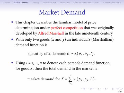
Market Demand● ais chapter describes the familiarmodel of price

determination under perfect competition that was originallydeveloped by AlfredMarshall in the late nineteenth century.

● With only two goods (x and y) an individual’s (Marshallian)demand function is

quantity of x demanded = x(px , py , I).

● Using i = 1,⋯, n to denote each person’s demand functionfor good x, then the total demand in themarket is

market demand for X =n∑i=1

xi(px , py , Ii).

4 / 34


aemarket demand curve

● To construct themarket demand curve for good X, we allowpx to vary while holding py and the income of eachindividual constant.

● aemarket demand curve is a “horizontal sum" of eachindividual’s demand curve.

● If each individual’s demand for x is downward sloping, themarket demand curve will also be downward sloping.

5 / 34


Figure 12.1 Construction of a Demand Curve from IndividualDemand Curves

6 / 34


Shi�s in theMarket Demand Curve

● aemarket demand summarizes the ceteris paribusrelationship between X and px .

● Changes in px result in movements along the curve (changein quantity demanded).

● Changes in other determinants of the demand for X causethe demand curve to shi� to a new position (change indemand).

7 / 34


Example 12.1 Shi�s in Market Demand

● Suppose that individual 1’s demand for oranges is given by:

x1 = 10 − 2px + 0.1I1 + 0.5py ,

where px is price of oranges, I1 is individual 1’s income. andpy is price of grapefruit.

● Individual 2’s demand for oranges is

x2 = 17 − px + 0.05I2 + 0.5py .

Hence, themarket demand function is

X(px , py , I1, I2) = x1 + x2 = 27 − 3px + 0.1I1 + 0.05I2 + py .

8 / 34


● If py = 4, I1 = 40, and I2 = 20, themarket demand curve is

X = 27 − 3px + 4 + 1 + 4 = 36 − 3px

● If py rises to 6, themarket demand curve shi�s outward to

X = 27 − 3px + 4 + 1 + 6 = 38 − 3px

● If I1 fell to 30 while I2 rose to 30, themarket demand wouldshi� inward to

X = 27 − 3px + 3 + 1.5 + 4 = 35.5 − 3px

9 / 34


Generalization

● Assume that there are m individuals in the economy, thenthe jth individual’s demand for the ith good will depend onall prices and on I j. ais can be denoted by

xi , j = xi , j(p1,⋯, pn , I j)

where i = 1,⋯, n and j = 1,⋯, n.

● Market demand. aemarket demand function for a good Xiis the sum of each individual’s demand for that good:

Xi(p1,⋯, pn , I1,⋯, Im) =m∑j=1

xi , j(p1,⋯, pn , I j)

● aemarket demand function depends on the prices of allgoods and the incomes and preferences of all buyers.

10 / 34


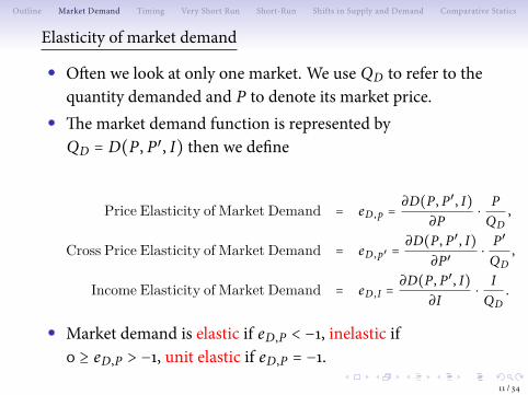
Elasticity ofmarket demand

● O�en we look at only onemarket. We use QD to refer to thequantity demanded and P to denote itsmarket price.

● aemarket demand function is represented byQD = D(P, P′, I) then we deûne

Price Elasticity of Market Demand = eD ,p =∂D(P, P′ , I)

∂P⋅

PQD

,

Cross Price Elasticity of Market Demand = eD ,p′ =∂D(P, P′ , I)

∂P′⋅

P′

QD,

Income Elasticity of Market Demand = eD ,I =∂D(P, P′ , I)

∂I⋅

IQD

.

● Market demand is elastic if eD,P < −1, inelastic if0 ≥ eD,P > −1, unit elastic if eD,P = −1.

11 / 34


Timing of the Supply Response

● It has been traditional in economics to discuss pricing inthree diòerent time period.

● In the very short run, there is no supply response.● In the short run, existing ûrmsmay change the quantity they

are supplying, but no new ûrms can enter the industry.● In the long run, new ûrmsmay enter an industry, thereby

producing a �exible supply response.

12 / 34


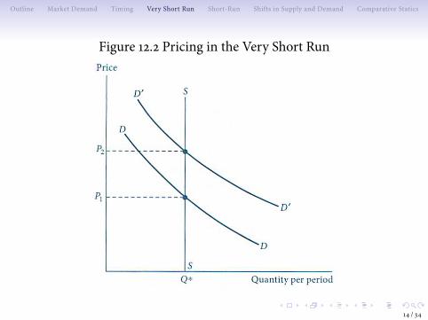
Pricing in the Very Short Run

● In the very short run, there is no supply response tochanging market conditions.

● Price acts only as a device for rationing demand. Price willadjust to clear themarket.

● ae supply curve is a vertical line.

13 / 34


Figure 12.2 Pricing in the Very Short Run

14 / 34


Short-Run Price Determination

● In the short-run, the number of ûrms in an industry is ûxed.● aese ûrms are able to adjust the quantity they are

producing in response to changing conditions.● aey can do this by altering the levels of the variable inputs

they employ.

15 / 34


Perfect competition. A perfectly competitivemarket is one thatobeys the following assumptions.

● aere are a large number of ûrms, each producing the samehomogeneous product.

● Each ûrm attempts to maximize proûts.● Each ûrm is a price taker: its actions have no eòect on the

market price.● Prices are assumed to be known by all market participants—

information is perfect.● Transactions are costless: Buyers and sellers incur no costs in

making exchanges (more in Chapter 18).

16 / 34


Short-run market supply curve

● ae quantity of output supplied to the entiremarket in theshort run is the sum of the quantities supplied by each ûrm.

● ae total amount supplied by each ûrm depends on theprice.

● ae relationship between price and quantity supplied iscalled short-runmarket supply curve.

● Because each ûrm’s short-run supply curve has a positiveslope, themarket supply curve will also have a positive slope.

17 / 34


Figure 12.3 Short-Run Market Supply Curve

18 / 34


Short-run market supply function● Short-run market supply function. ae short-run market

supply function shows total quantity supplied by each ûrm toamarket:

QS(P, v ,w) = S(P, v ,w) =n∑i=1

qi(P, v ,w),

where qi(P, v ,w) represent the short-run supply functionfor each of the n ûrms in the industry.

● Firms are assumed to face the samemarket price and thesame prices for inputs.

● ae short-run market supply curve shows thetwo-dimensional relationship between Q and P, holding vand w (and each ûrm’s technology) constant. If v ,w, ortechnology were to change, the supply curve would shi� to anew location.

19 / 34


Short-run supply elasticity

● Short-run supply elasticity describes the responsiveness ofquantity supplied to changes in market price.

● aismeasure shows how proportional changes in marketprice aremet by changes in total output.

eS , P =Percentage Change in Q supplied

Percentage Change in P= ∂QS

∂P⋅ PQS

.

● Because price and quantity supplied are positively related,eS , P > 0.

● High values for eS ,P imply that small increases in marketprice lead to a relatively large supply response by ûrmsbecausemarginal costs do not increase steeply and inputprice interaction eòects are small.

20 / 34


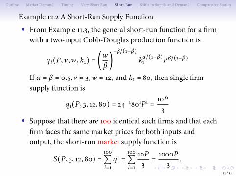
Example 12.2 A Short-Run Supply Function● From Example 11.3, the general short-run function for a ûrm

with a two-input Cobb-Douglas production function is

qi(P, v ,w , k1) = (wβ)−β/(1−β)

kα/(1−β)1 Pβ/(1−β)

If α = β = 0.5, v = 3,w = 12, and k1 = 80, then single ûrmsupply function is

qi(P, 3, 12, 80) = 24−1801P1 = 10P3

● Suppose that there are 100 identical such ûrms and that eachûrm faces the samemarket prices for both inputs andoutput, the short-run market supply function is

S(P, 3, 12, 80) =100∑i=1

qi =100∑i=1

10P3= 1000P

3.

21 / 34


● ae short-run elasticity of supply is

eS ,P =∂S(P, 3, 12, 80)

∂P⋅ PS= 1000

3⋅ P1000P/3 = 1.

● Eòect of an increase in w, Suppose wage increases to w = 15,the single ûrm’s supply function becomes

qi(P, 3, 15, 80) = 30−1801P1 = 8P3

and themarket supply function is

S(P, 3, 15, 80) =100∑i=1

8P3= 800P

3

At a price of P = 12, quantity supplied is QS = 3200, witheach ûrm producing qi = 32.

22 / 34


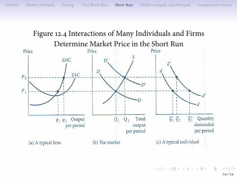
Equilibrium price determination

● Equilibrium price. An equilibrium price is one at whichquantity demanded is equal to quantity supplied. At such aprice, neither suppliers nor demanders have an incentive toalter their economic decisions. An equilibrium price (P∗)solves the equation

D(P∗, P′, I) = S(P∗, v ,w)

or,more compactly,

D(P∗) = S(P∗)

23 / 34


Figure 12.4 Interactions ofMany Individuals and FirmsDetermineMarket Price in the Short Run

24 / 34


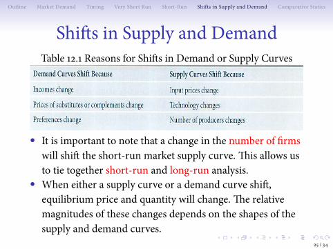
Shi�s in Supply and DemandTable 12.1 Reasons for Shi�s in Demand or Supply Curves

● It is important to note that a change in the number of ûrmswill shi� the short-run market supply curve. ais allows usto tie together short-run and long-run analysis.

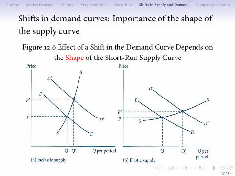
● When either a supply curve or a demand curve shi�,equilibrium price and quantity will change. ae relativemagnitudes of these changes depends on the shapes of thesupply and demand curves.

25 / 34


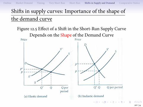
Shi�s in supply curves: Importance of the shape ofthe demand curve

Figure 12.5 Eòect of a Shi� in the Short-Run Supply CurveDepends on the Shape of the Demand Curve

26 / 34


Shi�s in demand curves: Importance of the shape ofthe supply curve

Figure 12.6 Eòect of a Shi� in the Demand Curve Depends onthe Shape of the Short-Run Supply Curve

27 / 34


A Comparative StaticsModel ofMarketEquilibrium

● Assume that the demand function is

QD = D(P, α)where α is an exogenous variable that shi�s the demandfunction such as income or the price of another good.

● ae short-run supply function is

QS = S(P, β),where β is an exogenous variable that shi�s the supplyfunction such as input prices or technical progress.

● Market equilibrium values P∗ and Q∗ are determined by

QD = QS = Q∗ = D(P∗, α) = S(P∗, β).28 / 34


● To show how these equilibrium values change when one ofthe exogenous variables changes, we write the equilibriumconditions as

D(P∗, α) − Q∗ = 0,

S(P∗, β) − Q∗ = 0.

Diòerentiate with respect α yields

DPdP∗dα+ Dα −

dQ∗dα

= 0, or DPdP∗dα− dQ∗

dα= −Dα

SPdP∗dα− dQ∗

dα= 0

29 / 34


● aese two equations can be written in matrix notation as

[ DP −1SP −1 ] ⋅

⎡⎢⎢⎢⎢⎣

dP∗dαdQ∗dα

⎤⎥⎥⎥⎥⎦= [ −Dα

0]

Applying Cramer’s rule to solve for dP∗/dα and dQ∗/dαyields

dP∗dα

=∣ −Dα −1

0 −1 ∣

∣ DP −1SP −1 ∣

= DαSP − DP

dQ∗dα

=∣ DP −DαSP 0

∣

∣ DP −1SP −1 ∣

= DαSPSP − DP

.

Since SP > 0,DP < 0, dP∗/dα and dQ∗/dα have the samesign as that of Dα . 30 / 34


An elasticity interpretation

● Multiply the equation for dP∗/dα by α/P∗ gives

ep∗ ,α =dP∗dα⋅ αP∗= DαSP − DP

⋅ αp∗= DαSP − DP

⋅ α/Q∗

p∗/Q∗ =eD,α

eS ,P − eD,P

● Similarly,multiplying the equation for α/Q∗ gives

eQ∗ ,α =dQ∗dα⋅ αQ∗= DαSPSP − DP

⋅ (α/Q∗)(P∗/Q∗)p∗/Q∗ = eD,α eS ,P

eS ,P − eD,P

● If supply were price elastic (eS ,P > 1) the proportionalincrease in equilibrium quantity would exceed theproportional increase in price.

● With an inelastic supply (eS ,P < 1) the situation would bereversed.

31 / 34


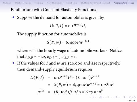
Equilibrium with Constant Elasticity Functions

● Suppose the demand for automobiles is given by

D(P, I) = 0.1P−1.2I3,

ae supply function for automobiles is

S(P,w) = 6, 400Pw−0.5

where w is the hourly wage of automobile workers. Noticethat eD,P = −1.2, eD,I = 3, eS ,P = 1.

● If the values for I and w are $20,000 and $25 respectively,then demand-supply equilibrium requires

D(P, I) = 0.1P−1.2I3 = (8 ⋅ 1011)P−1.2

= S(P,w) = 6, 400Pw−0.5 = 1, 280Pp2.2 = (8 ⋅ 1011)/1, 280 = 6.25 × 108

32 / 34


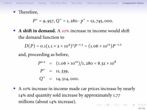
● aerefore,

P∗ = 9, 957,Q∗ = 1, 280 ⋅ p∗ = 12, 745, 000.

● A shi� in demand. A 10% increase in income would shi�the demand function to

D(P) = 0.1(1.1 × 2 × 104)3P−1.2 = (1.06 × 1012)P−1.2

and, proceeding as before,

P2.2 = (1.06 × 1012)/1, 280 = 8.32 × 108

P∗ = 11, 339,

Q∗ = 14, 514, 000.

● A 10% increase in incomemade car prices increase by nearly14% and quantity sold increase by approximately 1.77millions (about 14% increase).

33 / 34


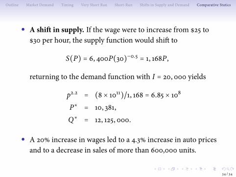
● A shi� in supply. If the wage were to increase from $25 to$30 per hour, the supply function would shi� to

S(P) = 6, 400P(30)−0.5 = 1, 168P,

returning to the demand function with I = 20, 000 yields

p2.2 = (8 × 1011)/1, 168 = 6.85 × 108

P∗ = 10, 381,

Q∗ = 12, 125, 000.

● A 20% increase in wages led to a 4.3% increase in auto pricesand to a decrease in sales ofmore than 600,000 units.

34 / 34

Documents

Part V: Competitiv Ma ˇ ae Partial Equ bri Competitive