Part I: A Quadratic Serendipity Plane Stress Element · A Quadratic Serendipity Plane Stress Element. ... •This last form is often known as Castigliano’s Second Theorem ... A

Putting It All TogetherMAE 323: Lecture 5

2011 Alex Grishin 1MAE 323 Lecture 5 Putting It All Together

Part I:

A Quadratic Serendipity

Plane Stress Element



Preliminaries: Energy Methods

•The first energy method to be used with FEM was the Rayleigh-Ritz

method. This method is based on the idea of minimizing the total

energy in a system by minimizing it’s variation, δ. This can be seen

in the example below

x0 x2

u(x0,0)

u(x2,0)

x1

u(x1,δ)=u(x1,0)+δu u(x1,δ)

u(x1,0)

A smoothly varying

function, u over the

domain x0≤x≤x2 may

be found by

minimizing all

smooth functions

u(x,δ) which equal

u(x,0) at x0 and x2

u(x1,0)

δu




•The parameter, δ may be thought of as a “virtual function” (or variation), and the

function, u is a function of this parameter (thus u(x,δ)-u(x,0)=δu(x) may be thought of as

a virtual displacement), as well as distance x

•Mathematically, the problem may be stated as:

Find the function, u for which the variation of the line integral, I for fixed x0,x2 is zero:

2

0

( ) ( , ',... ) 0x

xI x L u u x dxδ δ= =∫

OR:

0

0dI

d δδ =

=

(13)

(14)

•Applying (14) to (13) and integrating by parts leads to:

2

0 '

x

x

dI L d L udx

d u dx uδ δ

∂ ∂ ∂ = −

∂ ∂ ∂ ∫ (15)

where ' /u u x=∂ ∂




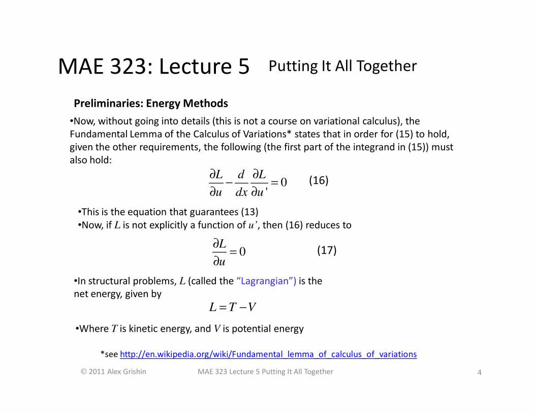
•Now, without going into details (this is not a course on variational calculus), the

Fundamental Lemma of the Calculus of Variations* states that in order for (15) to hold,

given the other requirements, the following (the first part of the integrand in (15)) must

also hold:

•This is the equation that guarantees (13)

•Now, if L is not explicitly a function of u’, then (16) reduces to

0'

L d L

u dx u

∂ ∂− =

∂ ∂

(17)

(16)

0L

u

∂=

∂

•In structural problems, L (called the “Lagrangian”) is the

net energy, given by

L T V= −

•Where T is kinetic energy, and V is potential energy

*see http://en.wikipedia.org/wiki/Fundamental_lemma_of_calculus_of_variations




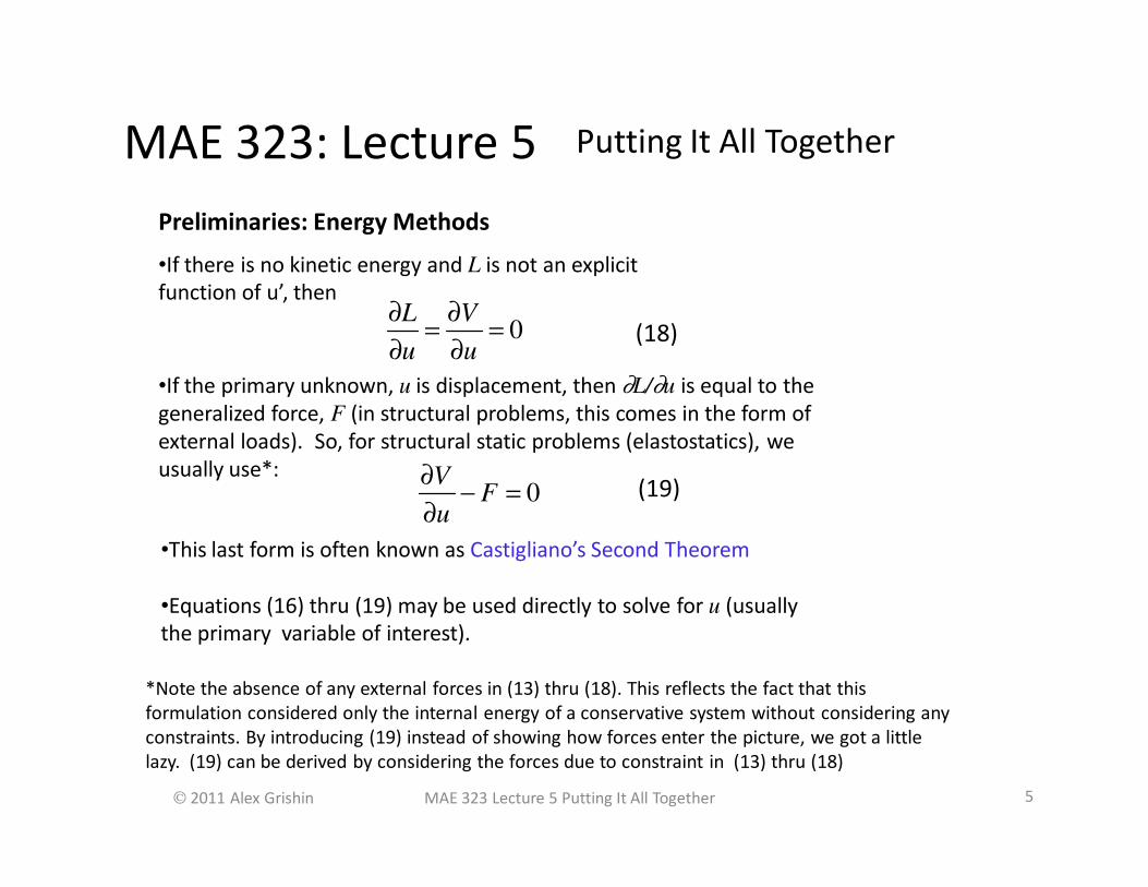
•If there is no kinetic energy and L is not an explicit

function of u’, then

(18)0L V

u u

∂ ∂= =

∂ ∂

•This last form is often known as Castigliano’s Second Theorem

•Equations (16) thru (19) may be used directly to solve for u (usually

the primary variable of interest).

•If the primary unknown, u is displacement, then ∂L/∂u is equal to the

generalized force, F (in structural problems, this comes in the form of

external loads). So, for structural static problems (elastostatics), we

usually use*:0

VF

u

∂− =

∂(19)

*Note the absence of any external forces in (13) thru (18). This reflects the fact that this

formulation considered only the internal energy of a conservative system without considering any

constraints. By introducing (19) instead of showing how forces enter the picture, we got a little

lazy. (19) can be derived by considering the forces due to constraint in (13) thru (18)




•To see how equation (19) is used, consider the simple case of a

spring, fixed at one end with an applied load F on the other

•First, write the expression for the potential energy:

•Now, substitute into equation (19):

21

2V ku=

0v

F ku Fu

∂− = − =

∂

•Hooke’s Law is recovered, and we can solve for u. In continuum and

reduced continuum problems, equation (19) will be an integral equation

(the energy distribution in a continuum is continuous!)



Preliminaries: Energy Methods . The Rayleigh-Ritz Method

•So, the Rayleigh-Ritz method is used by first finding an expression for the

potential energy of the discrete or continuous problem under investigation.

Then you plug into equation (19) and solve for u

•Below are some common expressions of potential energy found in structural

mechanics

2

0 2

L M dxV

EI= ∫

2

0 2

L S dxV

GA= ∫

2

0 2

L F dxV

EA= ∫

2

0 2

L T dxV

GJ= ∫

Symbols:M->Bending moment

S->Shear force

F->Tensile force

T->Torsion

A->Cross section area

E->Younng’s Modulus

G->Shear Modulus

{ε}->strain tensor in vector form*

{σ}->stress tensor in vector form*

A beam in bending A beam in shear A bar in tension A bar in torsion

{ } { }0 0 0

TW L T

dzdydxε σ∫ ∫ ∫

An elastic continuum*

* Here, second rank stress and strain tensors are expressed as vectors by

exploiting symmetry. This is often referred to as Voigt notation



Preliminaries: Energy Methods. The Rayleigh-Ritz Method

•Let’s try to reproduce Equation (8) – The equilibrium equations for a truss

element by using the Rayleigh-Ritz Method

•Start with the expression for potential energy in a bar (truss)2

0 2

L F dxV

EA= ∫

•Now, substitute the expressions for stress and strain (4a and 6a):

2

0 2

L

EAdudx

dxV

EA

= ∫

•Substitute your trial or shape functions*:

1 2

1

( ) 1n

i i

i

x xu x N u u u

L L=

= = − +

∑

*This is a major distinguishing feature of approximating energy methods. Instead of solving a

differential equation for u, we assume a polynomial solution a priori. This particular set of shape

functions happens to be the exact solution for the truss, but this is not a general requirement.




•Apply Castigliano’s Theorem (19) to obtain:

•Now evaluate using:

2

1 21 2

0 2

L

N NEA u u dx

x xV

EA

∂ ∂ +

∂ ∂ = ∫

( ) ( )( )' ' ' '

1 1 1 1 2 2 10

1

LVEA N N u N N u dx F

u

∂= + =

∂ ∫

( ) ( )( )' ' ' '

2 1 1 2 2 2 20

2

LVEA N N u N N u dx F

u

∂= + =

∂ ∫

'

1

'

2

1

1

NL

NL

−=

=

•Making the substitution:

1 1

2 2

1 1

1 1

u FEA

u FL

− =

−




•At this point, the student may not think anything has been gained (is the Rayleigh-

Ritz procedure really easier than the direct method?). However, we can omit

some steps if we observe that Castigiano’s Theorem always produces an equation

of the form*:

for one-dimensional elements, where C is the constitutive law, Ni, and Nj are

shape functions, and uj are the nodal coefficients

•This now provides a rule which can be easily (naively) used to generate algebraic

equations, which can then be solved numerically. Most importantly for us, it is

easily programmed

' '

1

n

i j j i

ji L

VN CN u F

u =

∂= =

∂∑∫ (20)

*Once again, note that there are no body loads in this formulation. Those must be

dealt with separately, or alternatively, one could use the Galerkin Method,

discussed next




T

V

V∂= ⋅ ⋅ =

∂ ∫∆ C ∆ d Fu

•In the most general case – that of an elastic continuum, we start with a

full strain matrix, and so, for a given element, Castigliano’s Theorem has

the form*:

where, for 3 dimensional isotropic materials, B , C, u and F are given by*:

0 0

0 0

0 0

0

0

0

x

y

z

y x

z y

z x

∂ ∂

∂ ∂

∂ ∂

∂ ∂ ∂ ∂

∂ ∂ ∂ ∂

∂ ∂ ∂ ∂

u

v

w

x

y

z

F

F

F

C ∆∆∆∆ d F

1 0 0 0

1 0 0 0

1 0 0 0

0 0 0 (1 2 ) / 2 0 0(1 )(1 2 )

0 0 0 0 (1 2 ) / 2 0

0 0 0 0 0 (1 2 ) / 2

E

ν ν ν

ν ν ν

ν ν ν

νν ν

ν

ν

−

− −

++ − −

−

(21)

*Students should recognize this as a matrix version of equation (2) of lecture 4 after

substitution of the Generalized Hooke’s Law



Preliminaries: Energy Methods. The Galerkin Method

•As we’ve seen, the Rayleigh-Ritz Method provides a formula, or template, for

generating stiffness matrices. For structural problems, it will always work.

However, for other types of boundary value problems, we may not always be able

to generate a Lagrangian (L) with all the required mathematical properties to

satisfy equations (16) thru (18)

•For these types of problems, another type of approximate energy method is

available. This method is more general than the Rayleigh-Ritz Method and is

equivalent to it in such situations when a proper Lagrangian function CAN be

obtained. This method involves constructing the weak form of the governing

differential equation.

•Because of it’s broad applicability and popularity, we will discuss this method next.




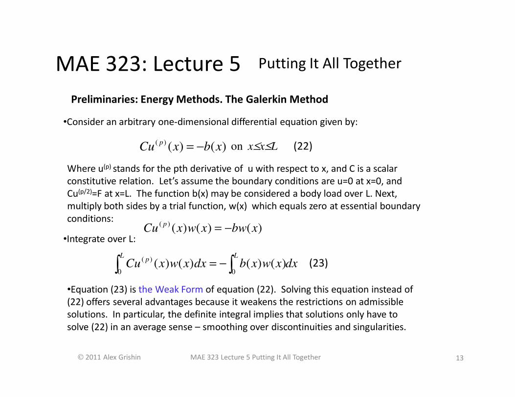
•Consider an arbitrary one-dimensional differential equation given by:

on x≤x≤L

Where u(p) stands for the pth derivative of u with respect to x, and C is a scalar

constitutive relation. Let’s assume the boundary conditions are u=0 at x=0, and

Cu(p/2)=F at x=L. The function b(x) may be considered a body load over L. Next,

multiply both sides by a trial function, w(x) which equals zero at essential boundary

conditions:

•Integrate over L:

( )( ) ( )

pCu x b x= −

( )( ) ( ) ( )

pCu x w x bw x= −

( )

0 0( ) ( ) ( ) ( )

L Lp

Cu x w x dx b x w x dx= −∫ ∫

(22)

(23)

•Equation (23) is the Weak Form of equation (22). Solving this equation instead of

(22) offers several advantages because it weakens the restrictions on admissible

solutions. In particular, the definite integral implies that solutions only have to

solve (22) in an average sense – smoothing over discontinuities and singularities.




•Next, use integration by parts:

(24)

•But, by the Fundamental Theorem of Calculus, the first term above is just equal to

the surface loads or tractions (remembering that w=0 at x=0):

•Substitute (24) into (23):

•Finally, this leaves us with:

(25)

( ) dxuxwxuxwdx

ddxxwxu

ppp

p

pp )2/()2/()2/(

2/

2/)(

)()()()()( ∫∫∫ −=

( ) ∫ ∫∫ −=−L L

ppL

p

p

p

dxxwxbdxxuxCwdxxuxwdx

dC

0 0

)2/()2/(

0

)2/(

2/

2/

)()()()()()(

( ) FLwxuxCwdxxuxwdx

dC

Lp

Lp

p

p

)()()()()(0

)2/(

0

)2/(

2/

2/

==∫

∫∫ +=LL

pp FLwdxxwxbdxxuxCw00

)2/()2/()()()()()(


2011 Alex Grishin

( ) ( ) ( ) FLNdxuxbNdxuxCNuxN i

L

iij

p

j

n

j

L

i

p

i )(0

)2/(

10

)2/(+= ∫∑∫

=

15MAE 323 Lecture 5 Putting It All Together


•For the discretized solution, we therefore substitute our chosen shape functions

for BOTH u and w:

Here, we go back to the notational shortcut, f(x) = f:

1

( ) ( )n

i i

i

u x N x u=

=∑

•In the Galerkin Method, the trial function, w is assumed to take the same form as

the solution, u

If there is no body load and (22) was a second order equation, we would have :

(26)

FLNdxbNdxuCNN i

L

ij

p

j

n

j

Lp

i )(0

)2/(

10

)2/( += ∫∑∫=

FLNdxuCNN ijj

n

j

L

i )('

10

' =∑∫=




•Thus, we see that the Galerkin procedure does indeed produce algebraic systems

equivalent to the Rayleigh-Ritz Method (at least for first-order differential

equations in one dimension).

•However, note a subtle difference produced by our assumptions. Let’s put the two

equations side-by-side:

•The difference appears in the external force vector on the RHS. In the Rayleigh-Ritz

Method, we started out with the assumption that all external tractions occur as nodal

point loads (via Castigliano’s Theorem). This is one way in which the Galerkin form is

more general in that it can accommodate any force vector, F distributed anywhere

within the domain (not just at nodes)!

•Multiplying such a vector by the shape function automatically weights it (lumps it) at

nodes. This is convenient for higher order, or higher dimensional problems

' '

1

n

i j j i

ji L

VN CN u F

u =

∂= =

∂∑∫ Rayleigh-Ritz

GalerkinFLNdxuCNN ijj

n

j

L

i )('

10

' =∑∫=



A Quadratic Serendipity Plane Stress Rectangular Element

•In Chapter 2, we learned two different energy-based methods of:

1. Turning differential equations into integral (or energy)

equations

2. Using this form of the equations to generate discrete

approximations using shape functions

•In Chapter 3, we learned how certain shape functions may be derived

•In Chapter 4, we learned some basic results from elasticity theory.

Namely, the form of the stress equilibrium equation and how stress

relates to strain via some form of Hooke’s Law

•In This chapter, we’d like to put all these ideas together to see how the

finite element method is used in a continuum problem




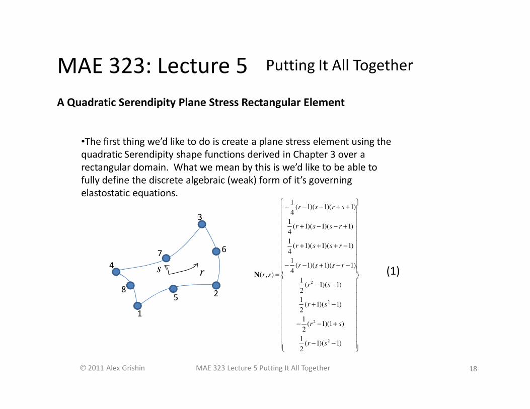
•The first thing we’d like to do is create a plane stress element using the

quadratic Serendipity shape functions derived in Chapter 3 over a

rectangular domain. What we mean by this is we’d like to be able to

fully define the discrete algebraic (weak) form of it’s governing

elastostatic equations.

2

2

2

2

1( 1)( 1)( 1)

4

1( 1)( 1)( 1)

4

1( 1)( 1)( 1)

4

1( 1)( 1)( 1)

4( , )

1( 1)( 1)

2

1( 1)( 1)

2

1( 1)(1 )

2

1( 1)( 1)

2

r s r s

r s s r

r s s r

r s s r

r s

r s

r s

r s

r s

− − − + + + − − + + + + −

− − + − −

= − − + −

− − +

− −

N (1)

2

1

rs

3

4

5

67

8



•Formally, the way we’d do this is to start with the differential equation

(from Chapter 4 – remembering that the indices range over spatial

coordinates):

,0

ij j ibσ + =

•Then, using the Galerkin formulation*, we would multiply this with a

trial function. In this context, it would be a vector-valued trial function,

wi

*Alternatively, we could integrate the strain energy density and equate this to the work

done by external nodal forces (i.e. the Rayleigh-Ritz Method)

( ),0

ij j i ib wσ + =

•Then integrate over an element volume

( ),0

ij j i i

V

b w dVσ + =∫





•Now, we won’t go through the complete derivation because it involves

some mathematics most students haven’t seen yet (mostly concepts

from Advanced Calculus). This is only because we are now working in

two spatial dimensions. We will just give the resulting weak form:

ij ij i i i i

V V S

t dV t b w t F w dSσ δε = +∫ ∫ ∫

where: ( ), ,

1

2ij i j j i

w wδε = +(see chapter 4 for the

definition of strain)

•And t is the thru-thickness (normal to the plane) of the domain.

Now replace the stress and strain tensors with their vector

counterparts (as well as the forces), as we saw in Chapter 4, and let’s

assume a unit thickness for t:

T

V V S

dV w wdSδ = +∫ ∫ ∫σ ε b F (2)

Stress

vector

Strain

vector

Body Load

vector

External surface

load vector



•Now, recall that the Serendipity elements are isoparametric, which

means that if we are going to perform the integrals in (2), we need an

explicit mapping between the isoparametric coordinates and the global

coordinates


rs

x

y

•For the strain matrix, this mapping is supplied

by the Jacobian of (x,y) with respect to (r,s):

x y

r r

x y

s s

∂ ∂ ∂ ∂

= ∂ ∂ ∂ ∂

J

such that:i ii

i ii

N NN x y

x xr r r

N NN x y

y ys ss

∂ ∂ ∂ ∂ ∂ ∂ ∂ ∂ ∂ ∂

= = ∂ ∂∂ ∂ ∂

∂ ∂ ∂ ∂∂

J (3)

1

2

3

4

5

67

8




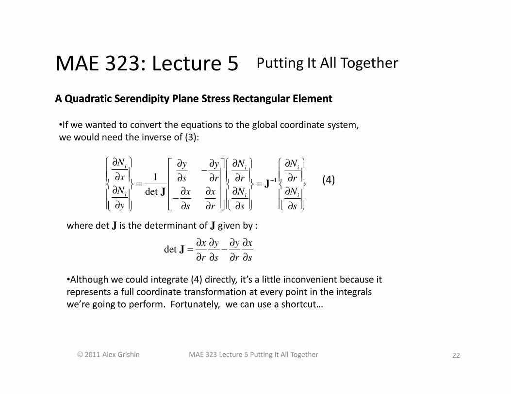
•If we wanted to convert the equations to the global coordinate system,

we would need the inverse of (3):


where det J is the determinant of J given by :

11

det

i i i

i i i

N N Ny y

x s r r r

N x x N N

y s r s s

−

∂ ∂ ∂∂ ∂ − ∂ ∂ ∂ ∂ ∂

= = ∂ ∂ ∂ ∂ ∂ −

∂ ∂ ∂ ∂ ∂

JJ

det x y y x

r s r s

∂ ∂ ∂ ∂= −

∂ ∂ ∂ ∂J

(4)

•Although we could integrate (4) directly, it’s a little inconvenient because it

represents a full coordinate transformation at every point in the integrals

we’re going to perform. Fortunately, we can use a shortcut…



A Quadratic Serendipity Plane Stress Rectangular ElementA Quadratic Serendipity Plane Stress Rectangular Element

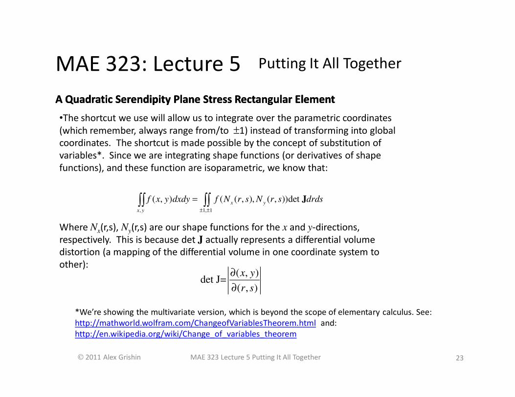
•The shortcut we use will allow us to integrate over the parametric coordinates

(which remember, always range from/to ±1) instead of transforming into global

coordinates. The shortcut is made possible by the concept of substitution of

variables*. Since we are integrating shape functions (or derivatives of shape

functions), and these function are isoparametric, we know that:


Where Nx(r,s), Ny(r,s) are our shape functions for the x and y-directions,

respectively. This is because det J actually represents a differential volume

distortion (a mapping of the differential volume in one coordinate system to

other):

, 1, 1

( , ) ( ( , ), ( , ))det x y

x y

f x y dxdy f N r s N r s drds± ±

=∫∫ ∫∫ J

( , )det J=

( , )

x y

r s

∂

∂

*We’re showing the multivariate version, which is beyond the scope of elementary calculus. See:

http://mathworld.wolfram.com/ChangeofVariablesTheorem.html and:

http://en.wikipedia.org/wiki/Change_of_variables_theorem



•Now, returning to the governing equations:


( )e e

e T e e

SV V

dV w wdSδ = +∫ ∫ ∫σ ε b F

•We are going to discretize this equation with our shape functions. We have

now attached a superscript e to all terms which will be evaluated on an element

basis. Before doing so, we make use of Hooke’s Law for an isotropic material to

convert the stress in the LHS to strain (we want the equation in terms of a single

primary unknown variable. In our case, this will be displacement):

( )e e

ee T e

SV V

dV wdV wdSδ = +∫ ∫ ∫ε C ε b F

•So, we need to write the strain vector in terms of shape functions. You already

got a hint of how we will do in this in Chapter 2. We’re going to write the strain

vector in term of a strain shape function matrix times displacement:

e e e e= ⋅ = ⋅ε B u ∆ d (6)

(5)



•B is the strain shape function matrix, and it is defined by:

•Where, ∆e is a strain operator. In the three dimensions, it is given as:

0 0

0 0

0 0

0

0

0

e

x

y

z

x y

z y

z x

∂ ∂

∂ ∂

∂ ∂

= ∂ ∂

∂ ∂

∂ ∂ ∂ ∂

∂ ∂ ∂ ∂

∆

e

u

v

w

=

d

e e e= ⋅B ∆ N (7)

e

=

N 0 0

N 0 N 0

0 0 N




•In two dimensions:


u

v

=

d

0

0e

x

y

y x

∂ ∂

∂ = ∂

∂ ∂ ∂ ∂

∆

•Substituting in our shape functions and converting to parametric coordinates:

0

0e

r

s

s r

∂ ∂

∂ = ∂

∂ ∂ ∂ ∂

∆

1

1

( , )

( , )

n

i i

ie

n

i i

i

N r s u

N r s v

=

=

=

∑

∑d

e⋅

= = ⋅

N u N 0 ud

N v 0 N vOr



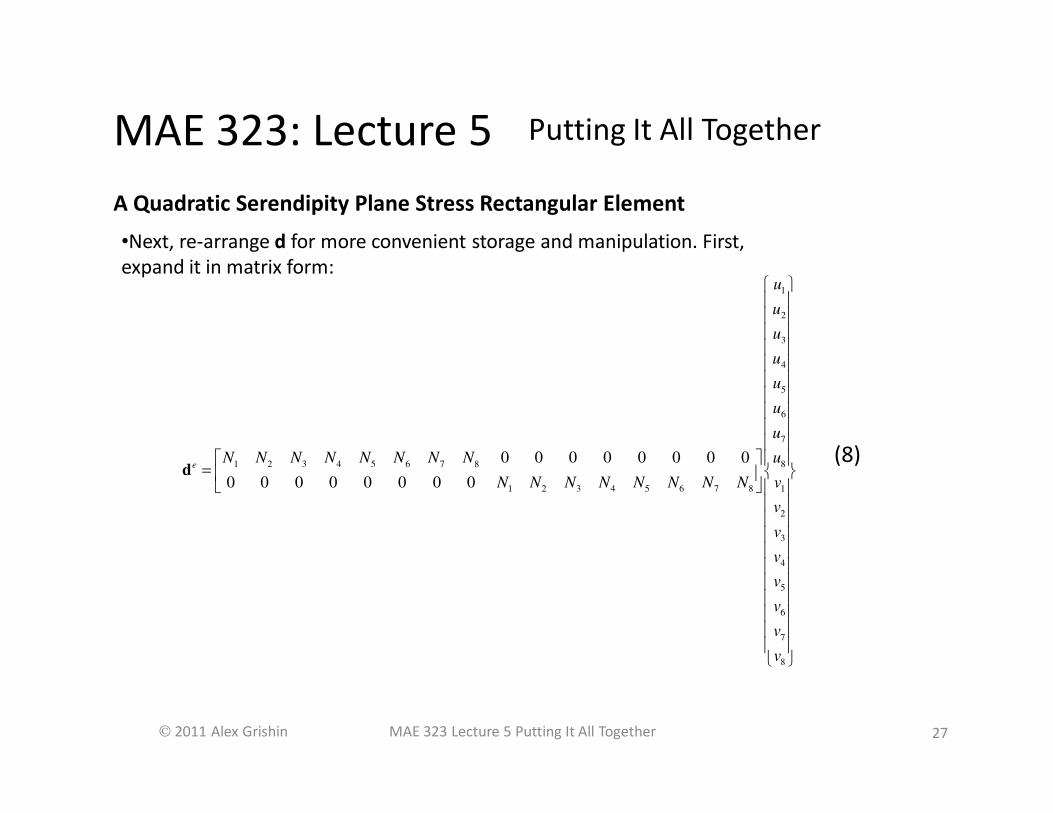
•Next, re-arrange d for more convenient storage and manipulation. First,

expand it in matrix form:


1

2

3

4

5

6

7

1 2 3 4 5 6 7 8 8

1 2 3 4 5 6 7 8 1

2

3

4

5

6

7

8

0 0 0 0 0 0 0 0

0 0 0 0 0 0 0 0

e

u

u

u

u

u

u

u

N N N N N N N N u

N N N N N N N N v

v

v

v

v

v

v

v

=

d(8)



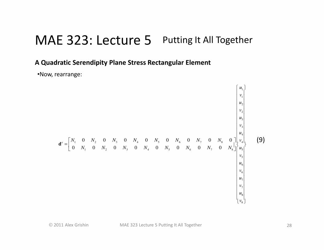
•Now, rearrange:


1

1

2

2

3

3

4

1 2 3 4 5 6 7 8 4

1 2 3 4 5 6 7 8 5

5

6

6

7

7

8

8

0 0 0 0 0 0 0 0

0 0 0 0 0 0 0 0

e

u

v

u

v

u

v

u

N N N N N N N N v

N N N N N N N N u

v

u

v

u

v

u

v

=

d(9)



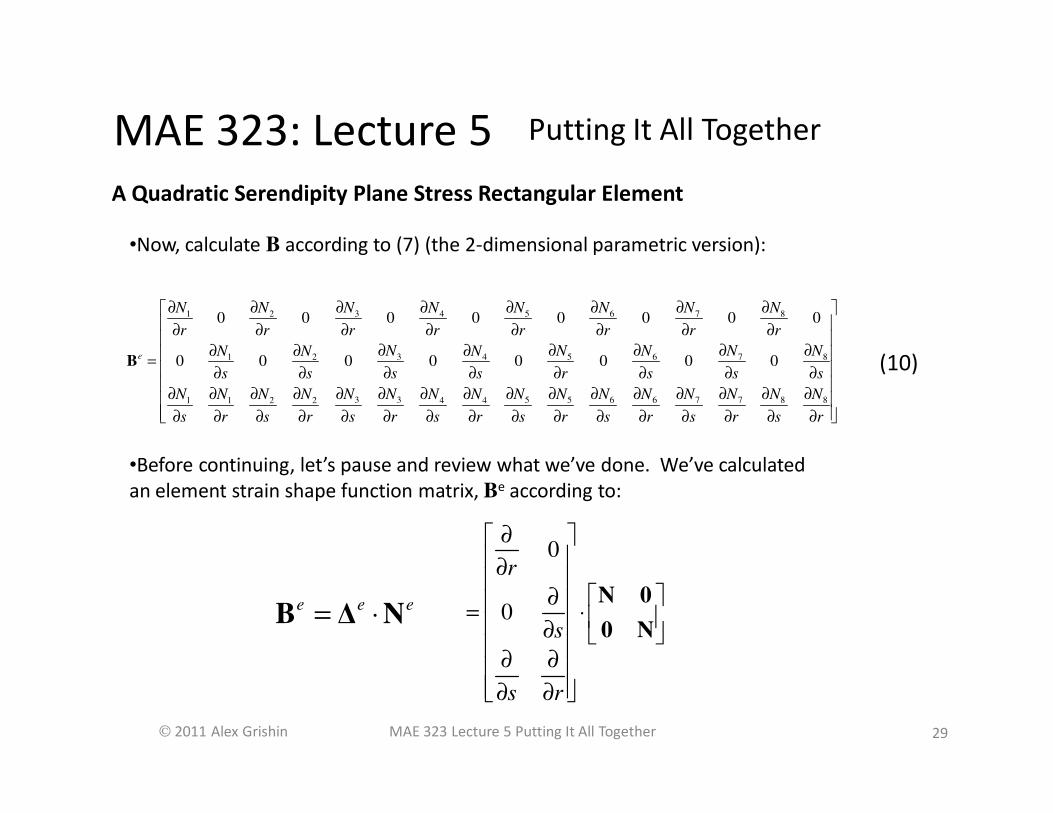
•Now, calculate B according to (7) (the 2-dimensional parametric version):


3 5 6 7 81 2 4

3 5 6 7 81 2 4

3 3 5 5 6 6 7 7 8 81 1 2 2 4 4

0 0 0 0 0 0 0 0

0 0 0 0 0 0 0 0e

N N N N NN N N

r r r r r r r r

N N N N NN N N

s s s s r s s s

N N N N N N N N N NN N N N N N

s r s r s r s r s r s r s r s r

∂ ∂ ∂ ∂ ∂∂ ∂ ∂ ∂ ∂ ∂ ∂ ∂ ∂ ∂ ∂

∂ ∂ ∂ ∂ ∂∂ ∂ ∂ = ∂ ∂ ∂ ∂ ∂ ∂ ∂ ∂

∂ ∂ ∂ ∂ ∂ ∂ ∂ ∂ ∂ ∂∂ ∂ ∂ ∂ ∂ ∂ ∂ ∂ ∂ ∂ ∂ ∂ ∂ ∂ ∂ ∂ ∂ ∂ ∂ ∂ ∂ ∂

B

•Before continuing, let’s pause and review what we’ve done. We’ve calculated

an element strain shape function matrix, Be according to:

e e e= ⋅B ∆ N

0

0

r

s

s r

∂ ∂

∂ = ⋅ ∂

∂ ∂ ∂ ∂

N 0

0 N

(10)



•So, we now have an expression of strain in terms of local parametric shape

functions:


•So, let’s go back to equation (5) and plug in what we’ve got so far:

e e e e e e= ⋅ = ⋅ ⋅ε B u ∆ N u

0

0

r

s

s r

∂ ∂

∂ = ⋅ ⋅ ∂

∂ ∂ ∂ ∂

N 0 u

0 N v

( ) ( ) ( )( ) det det det e e

ee e T e e e e e e

s

SV V

dV dV dS⋅ ⋅ ⋅ ⋅ = ⋅ ⋅ + ⋅ ⋅∫ ∫ ∫B u C B u J b N u J F N u J

( )e e

ee T e

SV V

dV wdV wdSδ = +∫ ∫ ∫ε C ε b F

(11)



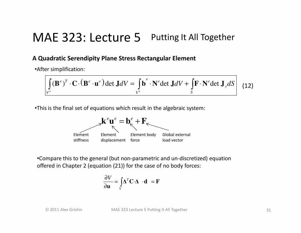
•After simplification:


( )( ) det det det e e

ee T e e e e

s

SV V

dV dV dS⋅ ⋅ ⋅ = ⋅ + ⋅∫ ∫ ∫B C B u J b N J F N J

•This is the final set of equations which result in the algebraic system:

e e e= +k u b F

Element

stiffness

Element

displacement

Element body

force

Global external

load vector

•Compare this to the general (but non-parametric and un-discretized) equation

offered in Chapter 2 (equation (21)) for the case of no body forces:

T

V

V∂= ⋅ ⋅ =

∂ ∫∆ C ∆ d Fu

(12)



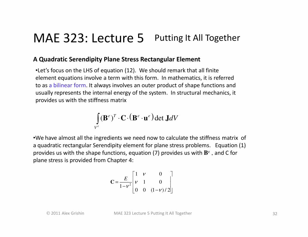
•Let’s focus on the LHS of equation (12). We should remark that all finite

element equations involve a term with this form. In mathematics, it is referred

to as a bilinear form. It always involves an outer product of shape functions and

usually represents the internal energy of the system. In structural mechanics, it

provides us with the stiffness matrix


( )( ) det e

e T e e

V

dV⋅ ⋅ ⋅∫ B C B u J

•We have almost all the ingredients we need now to calculate the stiffness matrix of

a quadratic rectangular Serendipity element for plane stress problems. Equation (1)

provides us with the shape functions, equation (7) provides us with Be , and C for

plane stress is provided from Chapter 4:

2

1 0

1 01

0 0 (1 ) / 2

Eν

νν

ν

= − −

C



•There’s still one thing missing! How do we calculate the integral over the

domain shown below?


( )( ) det e

e T e e

V

dV⋅ ⋅ ⋅∫ B C B u J

•This actually can be done analytically. Either manually or with a Computer Algebra

System (CAS). However, both techniques are too slow in general. What is needed is

a very accurate and robust (easily programmed and widely applicable) method of

doing this – even if it’s still only approximate.

•Historically, the method almost universally adopted is called Gaussian Quadrature,

which tends to give very good results for the integrals of smooth (or piecewise

smooth) functions

rs



•Gaussian Quadrature (sometimes called Legendre-Gauss Quadrature*) works

by sampling the integrand at points prescribed over the domain by the

quadrature rule. These points are then weighted and summed, producing the

an approximation of the integral.


Gaussian Quadrature

( ) ( )1 1

( ) det ( , ) ( , ) det ( , )e

n nT

e T e e e e

i j i j i j i j

i jV

dV r s r s r s w w= =

⋅ ⋅ ⋅ ≈ ⋅ ⋅∑∑∫ B C B u J B C B J

•The two-dimensional quadrature rule is generated by taking the outer product of

one-dimensional rules. Thus, if a three-point rule is used, the one dimension

locations, ri and corresponding weights, wi are found (looked up from a table or

calculated). The two dimensional points and weights are then found by the taking

the outer product of each (thus a three point rule results in nine points in two

dimensions, and 27 points in three dimensions).

*http://mathworld.wolfram.com/Legendre-GaussQuadrature.html



r

s

•Quadrature points are usually given on the interval -1<ri<1, and so this is

another convenience provided by the isoparametric coordinates

•Below the coordinates for a two-point rule are shown


Gaussian Quadrature

s

r

1/ 3s =

1/ 3s = −

1/ 3r = − 1/ 3r =



rs

•Below are the points for a three-point quadrature


Gaussian Quadrature

s

r

s

s

r=0.0

s

3 / 5s =

3 / 5s = −

3 / 5r =3 / 5r = −



•Below is a table of quadrature points and corresponding weights 2-point and 3-

point quadrature


Gaussian Quadrature

Point Locations Weights

2 -0.5773503 1.0000000

0.5773503 1.0000000

3 -0.7745967 0.5555556

0.0000000 0.8888889

0.7745967 0.5555556

•So, how do we know how many points to use when we integrate using

Gaussian Quadrature? The rules are derived (in one dimension) so as to

integrate all polynomials up to degree 2m-1 exactly, where m is the number of

points used in the quadrature! So, in principle, a 2-point rule would integrate

2nd and 3rd degree functions exactly.

1/ 3−

1/ 3

3 / 5−0

3 / 5

1

1

5 / 9

8 / 9

5 / 9



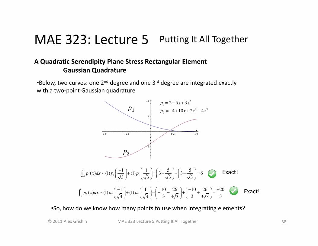
•Below, two curves: one 2nd degree and one 3rd degree are integrated exactly

with a two-point Gaussian quadrature


Gaussian Quadrature

•So, how do we know how many points to use when integrating elements?

p1

p2

2

1

2 3

2

2 5 3

4 10 2 4

p x x

p x x x

= − +

= − + + −

1

1 1 11

1 1( ) (1) (1) 3 3 6

3 3 3

5 5

3p x dx p p

−

− ≈ + = − + − =

∫

1

2 2 21

1 1 10 10 20( ) (1) (1)

3 3 33 3 3

26

3 3

26

3p x dx p p

−

− − − ≈ + = − − + + =

∫

Exact!

Exact!



•The guideline for exact integration is usually not followed in finite elements.

One reason is that for 2nd and 3rd degree shape functions, the preceding

formula would only be reliable if the sides of the rectangle were straight (if the

mid-side nodes lay on a straight line connecting corner nodes). When this is not

the case, we have a Jacobian with different values at all points within the

domain – this introduces error into the integral. Other reasons have to do with

mesh instabilities (which we’ll discuss later) and matrix assembly efficiency.

•In practice, a two-point quadrature rule is usually used for linear elements,

whereas a three-point rule is frequently used for quadratic elements.


Gaussian Quadrature



Part II:

Element Shape Quality

Metrics



•Element Distortion

•Whether creating a finite element mesh manually or using an automated program,

domain geometries which depart radically from the underlying element parent shape will

invariably lead to distorted elements (elements which themselves depart from their

parent shapes). This, in turn may lead to solution errors. The main reason for this lies in

the fact that the matrices for such elements become ill-conditioned. There are several

measures of element distortion. Some of the more common ones are:

•Aspect Ratio: A direct measure of departure from parent shape

•Angle Deviation: For quadrilateral and hexahedral elements. Measures

departure from 90 degree angle

•Parallel Deviation : Quadrilaterals and hexahedra only (dot product

between opposite edges calculated - must be close to zero)

•Maximum Corner Angle: For triangles, best possible max. angle in 60

degrees. For quadrilaterals, it’s 90 degrees.

•Jacobian Ratio: Jacobians determinants calculated at Gauss points,

corner nodes and centroid

•Warping Factor: A measure of twist for shell elements, but also for

solids



•Element Distortion

•The metric outlined in the previous slide are all used by ANSYS.

A description of how the code implements these metrics (as well

as explanations of the metrics themselves) can be found in the

ANSYS help documentation under Mechanical APDL->Theory

Reference->13. Element Shape Testing

Documents

Part I: A Quadratic Serendipity Plane Stress Element · A Quadratic Serendipity Plane Stress Element. ... •This last form is often known as Castigliano’s Second Theorem ... A