NASA/RSS SMAP Salinity: Version 4.0 Validated …...RSS Technical Report 082219 3 4.7 Antenna Pattern Correction (APC) 23 4.8 Ocean Target Calibration 24 5 SMAP SALINITY RETRIEVAL

RSS Technical Report 082219

1

RSS Technical Report 082219 August 22, 2019

NASA/RSS SMAP Salinity: Version 4.0 Validated Release Release Notes Algorithm Theoretical Basis Document (ATBD) Validation Data Format Specification

Thomas Meissner, Frank Wentz, Andrew Manaster, Richard Lindsley Remote Sensing Systems, Santa Rosa, CA

With contributions by: S. Grodsky (UMD), J. Vazquez (JPL), H.-Y. Kao (ESR), D. Levine (GSFC)


2

Table of Contents

1 SUMMARY 8

2 OVERVIEW OF V4.0 RELEASE 9

2.1 Release Date 9

2.2 Data Access 9

2.3 Citation and DOI 9

2.4 Summary of Updates and Improvements from V2.0 to V3.0 9

2.5 Summary of Updates and Improvements from V3.0 to V4.0 10

2.6 Latency 11

2.7 Spatial Resolution and Spatial Response Function 11

2.8 Known Issues 13

3 LEVEL 2 PROCESSING 14

3.1 Input 14

3.2 Optimum Interpolation (OI) onto Fixed Earth Grid (L2A) 14

3.3 Ancillary Fields (L2B) 14

3.4 Salinity Retrieval (L2C) 15

3.5 Reference Salinity Field 15

4 SMAP SALINITY RETRIEVAL ALGORITHM: VERSION 3 17

4.1 Overview and Basic Flow 17

4.2 Surface Roughness Correction 17 4.2.1 Ancillary Input for Wind Speed and Direction 17 4.2.2 Wind Induced Emissivity Model 18

4.3 Correction for Emissive SMAP Antenna 19

4.4 Atmospheric Oxygen Absorption 22

4.5 IMERG Rain Rate and Correction for Liquid Cloud Water Absorption 22

4.6 Correction for Reflected Galaxy 23


3

4.7 Antenna Pattern Correction (APC) 23

4.8 Ocean Target Calibration 24

5 SMAP SALINITY RETRIEVAL ALGORITHM: MAJOR UPDATES IN VERSION 4 26

5.1 Sidelobe Correction to Mitigate Land Intrusion 26 5.1.1 Computation of the SMAP Sidelobe Correction 26 5.1.2 Major Changes in the Version 4 Sidelobe Correction 26 5.1.3 Land Surface Emissivity 28 5.1.4 Additional Empirical Corrections 29 5.1.5 Land Exclusion for Calculating Smoothed Product 30 5.1.6 Results and Performance of Land Correction in Version 4.0 30

5.2 Revised Sun-Glint Flagging 32

5.3 Revised Sea-Ice Mask and Flagging 36

6 QUALITY CONTROL (Q/C) FLAGS 37

7 LEVEL 3 PROCESSING 39

7.1 Standard Product 39

7.2 Rain Filtered (RF) Product 39

7.3 Empirical Uncertainty Estimate 40

8 OPEN OCEAN PERFORMANCE ESTIMATE AND VALIDATION 41

8.1 Spatial Resolution and Noise Figures 41

8.2 Time Series of SMAP – ARGO – HYCOM Comparisons over the Open Ocean 41

8.3 Zonal and Average Regional Biases 44

9 REFERENCES 46

10 DATA FORMAT SPECIFICATION 48

10.1 Level 2C 48 10.1.1 Paths and Filenames 48 10.1.2 Global Attributes 48 10.1.3 Gridding and Dimensions 48 10.1.4 Variables 49

10.2 Level 3 52 10.2.1 Paths and Filenames 52


4

10.2.2 Global Attributes 53 10.2.3 Grid and Dimensions 53 10.2.4 Variables 53

APPENDIX A: BACKUS-GILBERT (BG) OPTIMUM INTERPOLATION (OI) 54


5

List of Figures

Figure 1: 1-dimensional cross section of spatial response functions (in dB): Blue: Gaussian gain pattern with half-power footprint diameter of 75 km. Red: Average of 3 Gaussian gain patterns whose half-power footprint diameters are 40 km each and who are centered at 0, +25 km, -25 km. .......................................................... 12

Figure 2: Flow diagram of the SMAP salinity retrieval algorithm. ............................................................................... 17

Figure 3: Left: Isotropic (wind-direction independent) part of the wind induced emissivity that is used in the Aquarius Version 5 after interpolating to the SMAP Earth Incidence Angle (dashed lines) and the SMAP Version 3 and Version 4 (full lines) releases. Blue: V-pol. Red: H-pol. The figure shows the 0th harmonic of the wind induced excess emissivity (Meissner et al. 2014, 2017) multiplied by 290 K. Right: SST dependence of the wind induced emissivity for Aquarius horn 2 H-pol. The blue line is the SST dependence from Meissner et al. 2014, which is predicted by the geometric optics model for the wind induced surface emission (Meissner et al. 2012). The red line is the SST dependence used in the Aquarius Version 5 release. The green line is the SST dependence used in the SMAP Version 3 and Version 4 releases (Meissner et al. 2018). ......... 18

Figure 4: Regression of TA measured minus expected versus binned Trefl – TA. Trefl is the physical temperature of the antenna (from the JPL thermal model). TA is the radiometric antenna temperature. Blue: V-pol. Red: H-pol. The slope of the linear fits is the reflector emissivity. The bin population (not shown) is very small at the lower and upper end of the x-axis interval, which causes the outliers. ............................................................. 20

Figure 5: Physical temperature Trefl of the reflector. Left: JPL thermal model that is used in the SMAP L1B files (Piepmeier et al. 2018). Right: Reflector temperature in the RSS SMAP Version 3 release after the empirical

adjustment refl

T has been added. .................................................................................................................... 20

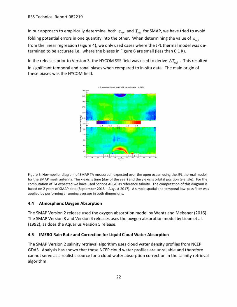
Figure 6: Hovmoeller diagram of SMAP TA measured - expected over the open ocean using the JPL thermal model for the SMAP mesh antenna. The x-axis is time (day of the year) and the y-axis is orbital position (z-angle). For the computation of TA expected we have used Scripps ARGO as reference salinity. The computation of this diagram is based on 2 years of SMAP data (September 2015 – August 2017). A simple spatial and temporal low-pass filter was applied by performing a running average in both dimensions. .......................... 22

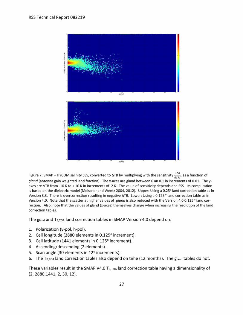
Figure 7: SMAP – HYCOM salinity SSS, converted to ΔTB by multiplying with the sensitivity 𝑑𝑇𝐵𝑑𝑆𝑆𝑆, as a function of gland (antenna gain weighted land fraction). The x-axes are gland between 0 an 0.1 in increments of 0.01. The y-axes are ΔTB from -10 K to + 10 K in increments of 2 K. The value of sensitivity depends and SSS. Its computation is based on the dielectric model (Meissner and Wentz 2004, 2012). Upper: Using a 0.25o land correction table as in Version 3.3. There is overcorrection resulting in negative ΔTB. Lower: Using a 0.125 o land correction table as in Version 4.0. Note that the scatter at higher values of gland is also reduced with the Version 4.0 0.125 o land correction. Also, note that the values of gland (x-axes) themselves change when increasing the resolution of the land correction tables. .................................................................................... 27

Figure 8: SMAP measured land TB minus land-emission model TB (based on NCEP soil moisture and land surface temperature). ..................................................................................................................................................... 28

Figure 9: SMAP – HYCOM salinity near Baja California (May 2018). Left: Version 3.0 70-km product. A large area near the coast was flagged for land contamination. Center: V3.3 70-km product. Right Version 4.0 smoothed product. .............................................................................................................................................................. 30

Figure 10: Statistics of RSS SMAP L2C versus ARGO match-ups as a function of gland. Left: V3.3. Right: V4.0. Median (white curve) and standard deviation (red curve). The colored shades indicate the 2-dimensional probability density. The analysis and figure were provided by H.-Y. Kao, ESR. ................................................ 31


6

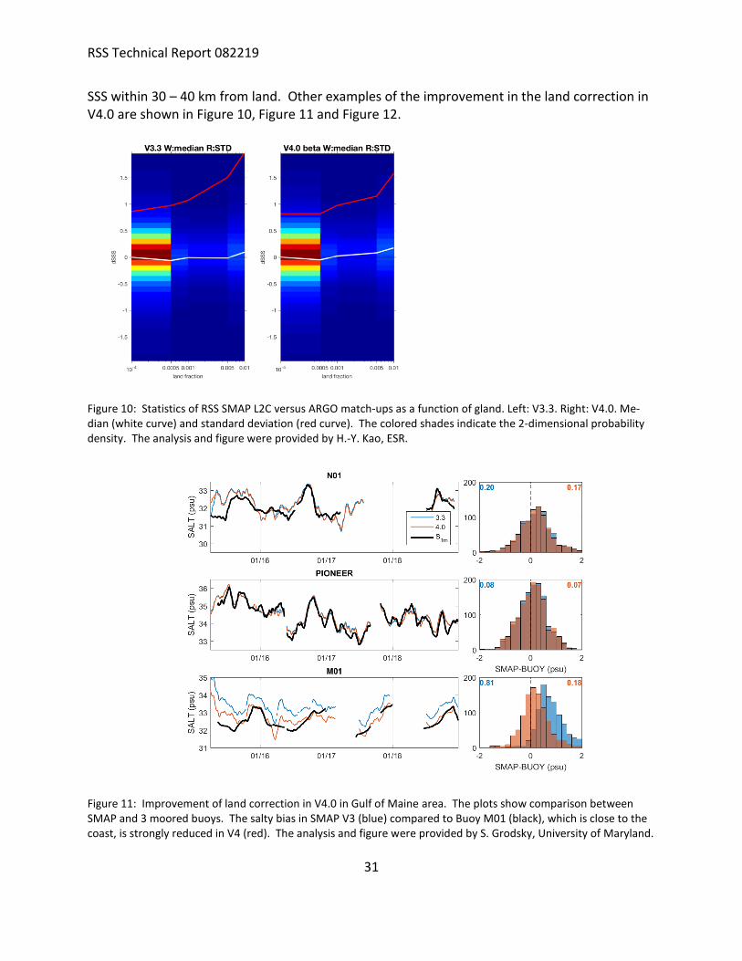
Figure 11: Improvement of land correction in V4.0 in Gulf of Maine area. The plots show comparison between SMAP and 3 moored buoys. The salty bias in SMAP V3 (blue) compared to Buoy M01 (black), which is close to the coast, is strongly reduced in V4 (red). The analysis and figure were provided by S. Grodsky, University of Maryland. ....................................................................................................................................................... 31

Figure 12: Comparison of SMAP SSS (8-day L3) and saildrone CTD salinity measurements during the Baja deployment (April 11 – June 11, 2018). For details see Vazquez-Cuervo et al. 2019. Upper: V3. Lower: V4. Black: saildrone. Red: SMAP. The fresh bias observed in V3 is greatly reduced in V4, in particular near Guadalupe Island. The analysis and figure were provided by J. Vazquez, JPL. ................................................. 32

Figure 13: The mean of the residual SSS as a function of sun glint angle and wind speed. Large magnitude errors are clamped for display purposes. The grey shaded area contains no data. .......................................................... 33

Figure 14: As Figure 13, but the V3 sun glint QC flag is used to mask out data. ......................................................... 34

Figure 15: As Figure 13, but with the revised sun glint QC flag for V4. ....................................................................... 34

Figure 16: The number of valid observations as a function of scan angle. The three cases are without the sun glint QC flag (purple), with the V3 sun glint QC flag (green), and with the revised V4 sun glint QC flag (blue). ....... 35

Figure 17: Similar to Figure 16, but the mean of the SSS residual as a function of scan angle for the three cases. ... 35

Figure 18: Similar to Figure 16, but the root-mean-square error of the SSS residual as a function of scan angle for the three cases. .................................................................................................................................................. 35

Figure 19: Coverage in the Antarctic fo RSS SMAP Salinity. Left: Version 3 using the NCEP sea-ice mask and a threshold for the gain weighted ice-fraction gice < 0.001. Right: Version 4 using the sea-ice mask from RSS AMSR2 (Wentz et al. 2014) and a threshold of gice < 0.003. ............................................................................. 36

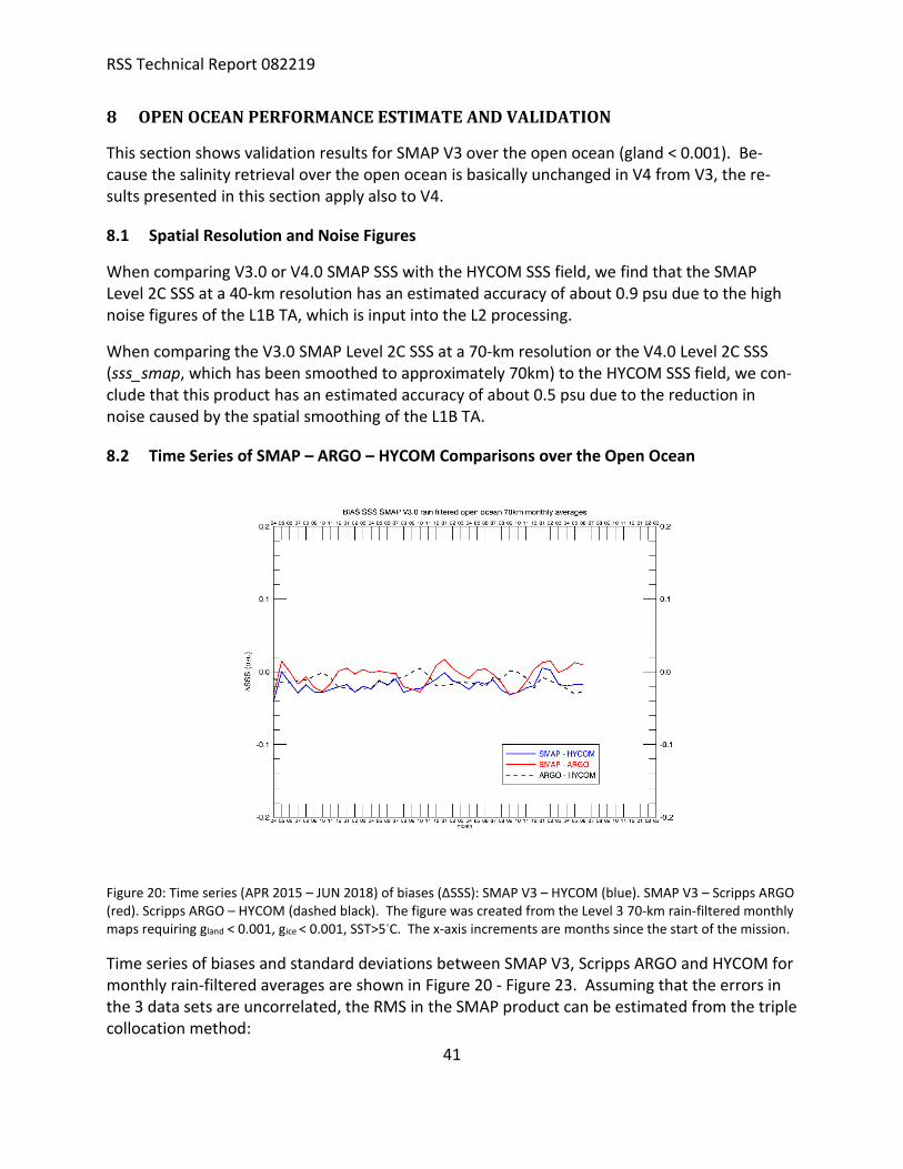
Figure 20: Time series (APR 2015 – JUN 2018) of biases (∆SSS): SMAP V3 – HYCOM (blue). SMAP V3 – Scripps ARGO (red). Scripps ARGO – HYCOM (dashed black). The figure was created from the Level 3 70-km rain-filtered monthly maps requiring gland < 0.001, gice < 0.001, SST>5◦C. The x-axis increments are months since the start of the mission. .................................................................................................................................................... 41

Figure 21: Time series (APR 2015 – JUN 2018) of standard deviations (∆SSS): SMAP V3 – HYCOM (blue). SMAP V3 – Scripps ARGO (red). Scripps ARGO – HYCOM (dashed black). The figure was created from the Level 3 70-km rain-filtered monthly maps requiring gland < 0.001, gice<0.001, SST>5◦C. The green curve is the estimated RMS error in the SMAP data based on the triple collocation method. The x-axis increments are months since the start of the mission. ..................................................................................................................................... 42

Figure 22: Same as Figure 21 for the 40-km product. ................................................................................................. 43

Figure 23: Same as Figure 21 for 1-deg lat/lon averages. ........................................................................................... 43

Figure 24: Hovmoeller diagram (APR 2015 – JUN 2018) of SMAP V3 SMAP V3 – Scripps ARGO. The figure was created from the Level 3 70-km rain-filtered monthly maps requiring gland < 0.001, gice < 0.001, SST>5◦C. The x-axis increments are months since the start of the mission. ............................................................................ 44

Figure 25: Global map (JAN 2016 – DEC 2017) of SMAP V3 SMAP V3 – Scripps ARGO. The figure was created from the Level 3 70-km rain-filtered monthly maps requiring gland < 0.001, gice < 0.001, SST>5◦C. ............................ 44


7

List of Tables

Table 1: List of dates with incomplete AMSR2 ancillary sea-ice mask. No L2 files are produced during these dates. L3 files that comprise these dates have a reduced number of observations in the time average. ................... 13

Table 2: Ancillary data sources. ................................................................................................................................... 14

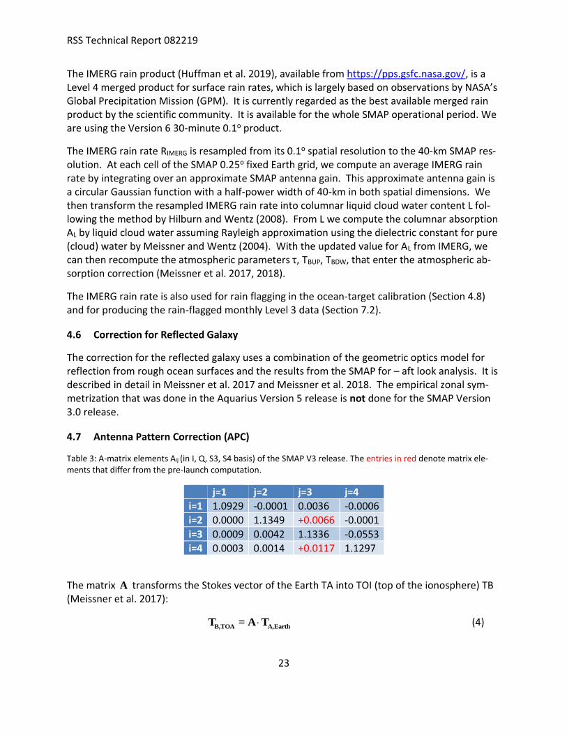
Table 3: A-matrix elements Aij (in I, Q, S3, S4 basis) of the SMAP V3 release. The entries in red denote matrix elements that differ from the pre-launch computation. ................................................................................... 23

Table 4: 32- bit Level 2 Q/C flags in the SMAP V4.0 release. ....................................................................................... 37


8

1 SUMMARY

This document contains the major steps of the NASA/RSS SMAP Version 3 and Version 4 salinity retrieval algorithm as well as the data format and specification of the NASA/RSS SMAP Version 4 release.

The major achievement in going from Version 2 to Version 3 is consistency with the Aquarius Version 5 end of mission release (Meissner et al. 2017, 2018) and the reduction of spurious temporal and zonal biases over the open ocean that had been observed in the SMAP Version 2 release.

The major change in Version 4 from Version 3 is an improved land correction, which allows to extend the SMAP salinity retrievals closer to the coast.

The standard product of the SMAP Version 4 release is the smoothed product with a spatial res-olution of approximately 70 km.


9

2 OVERVIEW OF V4.0 RELEASE

2.1 Release Date

07/22/2019

2.2 Data Access

www.remss.com/missions/smap/

https://podaac-opendap.jpl.nasa.gov/opendap/allData/smap/xx/RSS/V4/ xx = L2 or L3

Contact: Thomas Meissner, [email protected].

2.3 Citation and DOI

As a condition of using these data, we require you to use the following citation:

Meissner, T., F. J. Wentz, A. Manaster, R. Lindsley, 2019: Remote Sensing Systems SMAP Ocean Surface Salinities [Level 2C, Level 3 Running 8-day, Level 3 Monthly], Version 4.0 vali-dated release. Remote Sensing Systems, Santa Rosa, CA, USA. Available online at www.remss.com/missions/smap, doi: 10.5067/SMP40-xxxxx.

In the doi, the string xxxxx is:

1. 2SOCS for the L2C files. 2. 3SPCS for the L3 8-day running maps. 3. 3SMCS for the L3 monthly maps.

Continued production of this data set requires support from NASA. We need you to be sure to cite these data when used in your publications so that we can demonstrate its value to the sci-entific community. Please include the following statement in the acknowledgement section of your paper:

"SMAP salinity data are produced by Remote Sensing Systems and sponsored by the NASA Ocean Salinity Science Team. They are available at www.remss.com."

2.4 Summary of Updates and Improvements from V2.0 to V3.0

1. Use of Version 4 L1B SMAP RFI filtered antenna temperatures (Piepmeier et al. 2018). 2. Use of the GMF from Aquarius Version 5 Release adapted to SMAP (Meissner et al. 2017,

2018). 2.1. Use of Liebe et al. (1992) oxygen absorption model. 2.2. Use of surface roughness model from Meissner et al. 2014 with the adjustments speci-

fied in Meissner et al. 2018. For deriving the adjustments, the Scripps ARGO analyzed salinity is used as a reference.

http://www.remss.com/missions/smap/

https://podaac-opendap.jpl.nasa.gov/opendap/allData/smap/xx/RSS/V4/

mailto:[email protected]

http://www.remss.com/missions/smap

http://www.remss.com/


10

2.3. Galactic reflection model based on SMAP fore – aft look analysis (Meissner et al. 2017, 2018).

3. Use of CCMP near real time wind speed and direction as ancillary input. 4. Inclusion of IMERG rain rate. This is used in the atmospheric liquid cloud water correction

and for rain flagging. 5. Improved computation of antenna weighted land fraction gland. 6. Improved correction for the intrusion of land radiation from antenna sidelobes. 7. Emissive SMAP antenna:

7.1. The emissivity of the mesh antenna was set to 0.01012 for both V-pol and H-pol polari-zations.

7.2. The empirical adjustment to the JPL thermal model was rederived using the Scripps ARGO analyzed salinity field.

8. An error in the computation of the gain-weighted sea ice fraction gice during 2017 and 2018 in V2.0 has been corrected.

9. Antenna Pattern Correction (APC): The spillover, or equivalently the matrix element AII in the APC matrix, was decreased from 1.1080 (V2.0) to 1.0929 (V3).

10. The Level 2C (quality control) flags have been updated. 11. The salty biases at low latitudes and the fresh biases at high N latitudes that were observed

in the previous release have been significantly reduced in V3.0.

2.5 Summary of Updates and Improvements from V3.0 to V4.0

1. Improved land correction: The land tables in V4.0 are derived at 1/8o resolution. In V3.0 the spatial resolution of the land tables resolution had been ½o. The land surface TB that is used in the derivation of the land tables in V4.0 is based on a monthly climatology of SMAP land TB measurements. In V3.0 the land surface TB was based on a land surface emission model.

2. The sea-ice mask in V4.0 is taken from the RSS AMSR-2 sea-ice maps. In V3.0 the sea-ice mask was from NCEP. The threshold for sea-ice exclusion in V4.0 has been changed to gice > 0.003. This threshold was gice > 0.001 in V3.0.

3. The sun-glint flag has been revised. In V4.0 the sun-glint exclusion is based on sun-glint an-gle and surface wind speed. The V4.0 sun-glint flag excludes less data then the V3.0 flag did.

4. The Version 4.0 salinity retrieval algorithm is run solely on the 0.25o Earth grid using the 40-km spatial resolution Backus Gilbert Optimum Interpolation (OI). The resulting salinity product is called sss_smap_40km. From this 40-km product, a smoothed product with a spatial resolution of approximately 70km (called sss_smap) is derived using simple next-neighbor averaging. This smoothed 70-km sss_smap is to be regarded as the default (standard) salinity product. In Version 4, both sss_smap and sss_smap_40km are provided in the same file.


11

5. An empirical uncertainty estimate sss_smap_uncertainty is provided for sss_smap in the Level 3 files. This uncertainty is based on comparisons between SMAP and the Scripps ARGO interpolated fields. This also includes the sampling error of the Argo data on the scales of the gridded maps, as well as the mapping errors.

2.6 Latency

• L2C: 24 – 48-hour latency.

• L3 8-day running average: 3-day latency (after the end of the averaging period).

• L3 monthly average: 3-day latency (after the end of the averaging period).

2.7 Spatial Resolution and Spatial Response Function

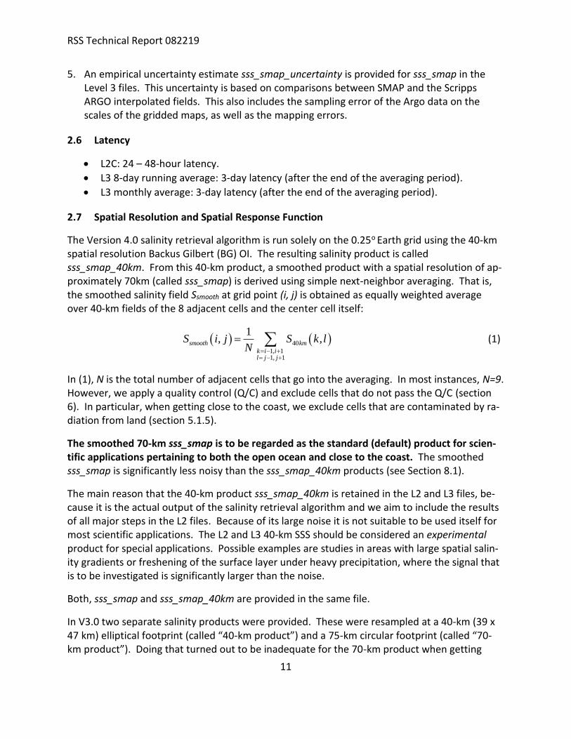
The Version 4.0 salinity retrieval algorithm is run solely on the 0.25o Earth grid using the 40-km spatial resolution Backus Gilbert (BG) OI. The resulting salinity product is called sss_smap_40km. From this 40-km product, a smoothed product with a spatial resolution of ap-proximately 70km (called sss_smap) is derived using simple next-neighbor averaging. That is, the smoothed salinity field Ssmooth at grid point (i, j) is obtained as equally weighted average over 40-km fields of the 8 adjacent cells and the center cell itself:

( ) ( )40

1, 11, 1

1, ,smooth km

k i il j j

S i j S k lN = − +

= − +

= (1)

In (1), N is the total number of adjacent cells that go into the averaging. In most instances, N=9. However, we apply a quality control (Q/C) and exclude cells that do not pass the Q/C (section 6). In particular, when getting close to the coast, we exclude cells that are contaminated by ra-diation from land (section 5.1.5).

The smoothed 70-km sss_smap is to be regarded as the standard (default) product for scien-tific applications pertaining to both the open ocean and close to the coast. The smoothed sss_smap is significantly less noisy than the sss_smap_40km products (see Section 8.1).

The main reason that the 40-km product sss_smap_40km is retained in the L2 and L3 files, be-cause it is the actual output of the salinity retrieval algorithm and we aim to include the results of all major steps in the L2 files. Because of its large noise it is not suitable to be used itself for most scientific applications. The L2 and L3 40-km SSS should be considered an experimental product for special applications. Possible examples are studies in areas with large spatial salin-ity gradients or freshening of the surface layer under heavy precipitation, where the signal that is to be investigated is significantly larger than the noise.

Both, sss_smap and sss_smap_40km are provided in the same file.

In V3.0 two separate salinity products were provided. These were resampled at a 40-km (39 x 47 km) elliptical footprint (called “40-km product”) and a 75-km circular footprint (called “70-km product”). Doing that turned out to be inadequate for the 70-km product when getting


12

close to land. The BG OI (Appendix A) results in a weighted average of the SMAP observations in the neighborhood of the target cell. Close to land, some of these surrounding cells are con-taminated by radiation land, which is difficult to deal with.

Over the open ocean, the differences between the BG OI in the Version 3 70-km product and the smoothed Version 4 product are small. In Figure 1, we have used a simplified 1-dimensional model to compare the spatial response (gain) of a 75-km 1-dimensional Gaussian footprint (blue) with the one obtained by averaging three 1-dimensional Gaussian 40-km footprints that

are centered at -25 km, 0, +25 km (red). If ( )40kmg x denotes 1-dimensional Gaussian footprint

with a half-power (3dB) width of 40km centered at 0x = , then the red curve ( )smoothg x in Fig-

ure 1 is obtained as:

( ) ( ) ( ) ( )40 40 40

125 25

3smooth km km kmg x g x g x g x= − + + + (2)

This corresponds to the smoothing procedure in equation (1) for the simplified case of 1 spatial

dimension. The blue curve in Figure 1 is the 1-dimensional Gaussian footprint ( )75kmg x with a

half-power width of 75 km. The blue and red curves in have approximately the same half-

power widths, that is with in the mainlobe: ( ) ( )75smooth kmg x g x . The smoothed sss_smap in

V4.0 has approximately the same noise reduction as the 70-km sss_smap in V3.0.

Figure 1: 1-dimensional cross section of spatial response functions (in dB): Blue: Gaussian gain pattern with half-power footprint diameter of 75 km. Red: Average of 3 Gaussian gain patterns whose half-power footprint diame-ters are 40 km each and who are centered at 0, +25 km, -25 km.


13

2.8 Known Issues

1. We observe a significant degradation in retrieval performance during the early months of the SMAP mission (APR 2015 – AUG 2015). This might be related to instrument calibration, but the exact cause is currently unknown and needs further investigation. See Section 8.2 for more information.

2. The ancillary RSS AMSR2 sea-ice mask (section 5.3) is incomplete during a few days. In or-der to avoid possible contamination from sea-ice, no SMAP salinity retrievals are done in these cases. Consequently, the L3 products that comprise these dates contain are produced with a reduced number of observations in the time average. The following dates have been identified:

Table 1: List of dates with incomplete AMSR2 ancillary sea-ice mask. No L2 files are produced during these dates. L3 files that comprise these dates have a reduced number of observations in the time average.

year Month Day Day of year

2015 12 3 337

2015 12 4 338

2016 4 15 106

2016 4 16 107

2017 9 27 270

2017 9 28 271

2017 11 25 329

2018 12 16 350


14

3 LEVEL 2 PROCESSING

3.1 Input

The RSS SMAP salinity retrieval algorithm ingests RFI filtered antenna temperatures (TA) from the Version 4 SMAP L1B data files (Piepmeier et al., 2018) together with basic spacecraft ephemeris information (S/C location, velocity, and attitude) and time of observation.

3.2 Optimum Interpolation (OI) onto Fixed Earth Grid (L2A)

As a first step, we perform a Backus-Gilbert (BG) type optimum interpolation (OI) (Stogryn 1978, Poe 1990) and resample the L1B TA onto a fixed 0.25o Earth grid at approximately 40-km spatial resolution. For details see Appendix A. The resulting gridded TAs are known as Level 2A files. The resampling is done separately for the forward (for) and the backward (aft) look. This 40-km product (sss_smap_40km) maintains the approximate spatial resolution and shape (39 km x 47 km) of the original SMAP L1B swath observations (Piepmeier et al., 2018). The final V4.0 smoothed sss_smap is obtained at each of the 0.25o cells from the sss_smap_40km field by averaging the cell with the 8 adjacent 0.25o cells together. This smoothed V4.0 sss_smap field is the default product for science applications.

3.3 Ancillary Fields (L2B)

The ancillary sources for the V4.0 Level 2 processing are listed in Table 2. The ancillary fields are space-time interpolated to the location and time of the L2A data in order to create Level 2B files.

Table 2: Ancillary data sources.

Ancillary Input Data Source sea surface temperature

Canadian Meteorological Center. 2016 GHRSST Level 4 CMC 0.2deg Global Foun-dation Sea Surface Temperature Analysis. Version. 3.0. doi: 10.5067/GHCMC-4FM03, http://dx.doi.org/10.5067/GHCMC-4FM03.

sea surface wind speed and direction

CCMP V2.0 near-real time wind speed and direction. http://www.remss.com/measurements/ccmp/. (Mears et al. 2018).

atmospheric profiles for pres-sure, height, temperature, rela-tive humidity, cloud water mix-ing ratio

NCEP GDAS 1-deg 6-hour. HGT, PRS, TMP, TMP, RH, CLWMR. Available from https://nomads.ncep.noaa.gov/.

IMERG rain rate Huffman, G. et al., 2019. NASA Global Precipitation Measurement (GPM) Inte-grated Multi-Satellite Retrievals for GPM (IMERG) Version 6, LATE RUN, 30-minutes, NASA, http://dx.doi.org/10.5067/GPM/IMERG/3B-HH/06.

solar flux Noon flux values from US Air Force Radio Solar Telescope sites 1415 MHz values. Available from NOAA Space Weather Prediction Center, www.swpc.noaa.gov.

total electron content (TEC) IGS IONEX TEC files. Available from ftp://cddis.gsfc.nasa.gov/pub/gps/products/ionex/.

http://dx.doi.org/10.5067/GHCMC-4FM03

http://www.remss.com/measurements/ccmp/

https://nomads.ncep.noaa.gov/

http://www.swpc.noaa.gov/

ftp://cddis.gsfc.nasa.gov/pub/gps/products/ionex/


15

sea ice fraction RSS AMSR2 sea-ice mask (Wentz et al. 2014). Available from www.remss.com/amsr/.

land mask 1 km land/water mask from OCEAN DISCIPLINE PROCESSING SYSTEM (ODPS). Based on the World Vector Shoreline (WVS) database and World Data Bank. Cour-tesy of Fred Patt, Goddard Space Flight Center, [email protected].

galactic map Dinnat, E.; Le Vine, D.; Abraham, S.; Floury, N. Map of Sky Background Brightness Temperature at L-Band. 2018. Available online at https://podaac-tools.jpl.nasa.gov/drive/files/allData/aquarius/L3/mapped/galaxy/2018.

reference salinity (HYCOM) in the ocean target calibration

Hybrid Coordinate Ocean Model, GLBa0.08/expt_90.9, Top layer salinity. Available at www.hycom.org.

Scripps ARGO salinity (only included in rain-filtered L3 monthly files)

monthly 1-degree gridded interpolated ARGO SSS field provided by Scripps. Available at www.Argo.ucsd.edu/Gridded_fields.html.

The ancillary TEC maps are not used anywhere in in the actual salinity retrieval algorithm. As it was the case for the Aquarius salinity retrieval algorithm (Meissner et al. 2017), the Faraday ro-tation correction in the SMAP salinity retrieval uses the measured 3rd Stokes parameter S3. The ancillary TEC values can be used to check the calibration of S3 by comparing the measured Fara-day rotation with the computation based on the ancillary TEC field.

The Scripps ARGO salinity in the monthly rain-filtered L3 files are not used anywhere in the ac-tual salinity retrieval algorithm. They are included to facilitate comparison of the rain-filtered SMAP salinity with the Scripps ARGO field.

3.4 Salinity Retrieval (L2C)

The SMAP salinity retrieval algorithm is then run on these Level 2B files and produces calibrated SMAP Level 2C surface ocean brightness temperatures (TB) and sea surface salinity (SSS) values.

3.5 Reference Salinity Field

When running the Aquarius and SMAP salinity retrieval algorithms, a reference salinity field is needed for the ocean target calibration (section 4.8). The ocean target calibration ensures that the global average of the Aquarius or SMAP salinity matches the global average of the refer-ence salinity field. For the Aquarius V5 end of mission release, the Scripps ARGO field has been used as reference salinity field in the ocean target calibration. Because of the long latency of the Scripps ARGO field this is not feasible for SMAP, which is an active mission. Therefore, for SMAP the HYCOM field is used as reference salinity field in the ocean target calibration. The global average between Scripps ARGO and HYCOM are very small, in the order of 0.02 psu, and therefore the choice between Scripps ARGO and HYOM is marginal for the ocean target calibra-tion.

When developing the SMAP salinity retrieval algorithm, we also need a reference salinity for the surface roughness correction (section 4.2) and the adjustment to the thermal model for the reflector in the correction for the emissive antenna (section 4.3). The derivation of these cor-rections do not require a dynamical update. For the SMAP Version 3 and Version 4 releases we

http://www.remss.com/amsr/

mailto:[email protected]

https://podaac-tools.jpl.nasa.gov/drive/files/allData/aquarius/L3/mapped/galaxy/2018

https://podaac-tools.jpl.nasa.gov/drive/files/allData/aquarius/L3/mapped/galaxy/2018

http://www.hycom.org/

http://www.argo.ucsd.edu/Gridded_fields.html


16

are using the Scripps ARGO field as reference salinity. In the Version 1 and Version 2 releases, HYCOM has been used for these cases. It turned out to be inadequate as the HYCOM field has significant temporal and zonal biases when compared to in-situ data. These HYCOM biases are then also visible in the SMAP salinity retrievals. Removing these biases has been a major step going from Version 2 to Version 3 and using Scripps ARGO instead of HYCOM in the wind emis-sivity model and the thermal reflector adjustment played a crucial role (see sections 2.4 and 8.3).


17

4 SMAP SALINITY RETRIEVAL ALGORITHM: VERSION 3

4.1 Overview and Basic Flow

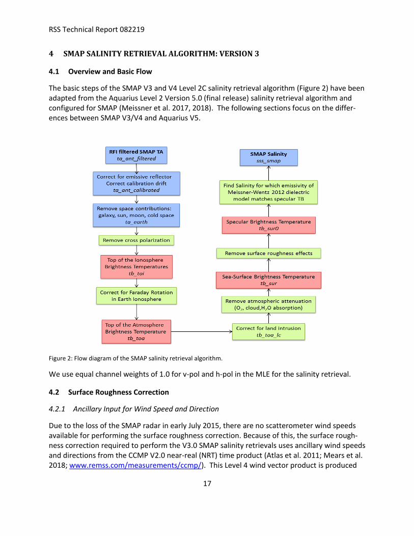
The basic steps of the SMAP V3 and V4 Level 2C salinity retrieval algorithm (Figure 2) have been adapted from the Aquarius Level 2 Version 5.0 (final release) salinity retrieval algorithm and configured for SMAP (Meissner et al. 2017, 2018). The following sections focus on the differ-ences between SMAP V3/V4 and Aquarius V5.

Figure 2: Flow diagram of the SMAP salinity retrieval algorithm.

We use equal channel weights of 1.0 for v-pol and h-pol in the MLE for the salinity retrieval.

4.2 Surface Roughness Correction

4.2.1 Ancillary Input for Wind Speed and Direction

Due to the loss of the SMAP radar in early July 2015, there are no scatterometer wind speeds available for performing the surface roughness correction. Because of this, the surface rough-ness correction required to perform the V3.0 SMAP salinity retrievals uses ancillary wind speeds and directions from the CCMP V2.0 near-real (NRT) time product (Atlas et al. 2011; Mears et al. 2018; www.remss.com/measurements/ccmp/). This Level 4 wind vector product is produced

http://www.remss.com/measurements/ccmp/


18

daily at RSS using variational assimilation (VAM) of different satellite wind products and a back-ground wind field. The spatial gridding is 0.25o x 0.25o and the time resolution is 6-hours (00Z, 06Z, 12Z, 18Z). The V2.0 NRT CCMP assimilates RSS wind speed and wind direction measure-ments from the RSS Version 7/8 ocean suite, which includes data from the following sensors: WindSat, SSMIS F16, F17, F18, GMI, and AMSR2. Because of latency, observations from RSS ASCAT and from buoys are not ingested into the V2.0 NRT CCMP processing. The background wind field that is used in the CCMP VAM is the 0.25o field from NCEP GDAS (https://no-mads.ncep.noaa.gov/).

4.2.2 Wind Induced Emissivity Model

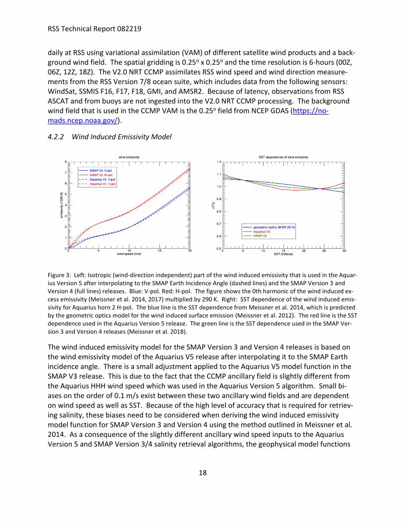
Figure 3: Left: Isotropic (wind-direction independent) part of the wind induced emissivity that is used in the Aquar-ius Version 5 after interpolating to the SMAP Earth Incidence Angle (dashed lines) and the SMAP Version 3 and Version 4 (full lines) releases. Blue: V-pol. Red: H-pol. The figure shows the 0th harmonic of the wind induced ex-cess emissivity (Meissner et al. 2014, 2017) multiplied by 290 K. Right: SST dependence of the wind induced emis-sivity for Aquarius horn 2 H-pol. The blue line is the SST dependence from Meissner et al. 2014, which is predicted by the geometric optics model for the wind induced surface emission (Meissner et al. 2012). The red line is the SST dependence used in the Aquarius Version 5 release. The green line is the SST dependence used in the SMAP Ver-sion 3 and Version 4 releases (Meissner et al. 2018).

The wind induced emissivity model for the SMAP Version 3 and Version 4 releases is based on the wind emissivity model of the Aquarius V5 release after interpolating it to the SMAP Earth incidence angle. There is a small adjustment applied to the Aquarius V5 model function in the SMAP V3 release. This is due to the fact that the CCMP ancillary field is slightly different from the Aquarius HHH wind speed which was used in the Aquarius Version 5 algorithm. Small bi-ases on the order of 0.1 m/s exist between these two ancillary wind fields and are dependent on wind speed as well as SST. Because of the high level of accuracy that is required for retriev-ing salinity, these biases need to be considered when deriving the wind induced emissivity model function for SMAP Version 3 and Version 4 using the method outlined in Meissner et al. 2014. As a consequence of the slightly different ancillary wind speed inputs to the Aquarius Version 5 and SMAP Version 3/4 salinity retrieval algorithms, the geophysical model functions

http://nomads.ncep.noaa.gov/

http://nomads.ncep.noaa.gov/


19

for the wind emissivities also differ slightly. This is most important for the wind speed depend-ence 0th harmonic coefficient of the wind induced emissivity i.e., the isotropic part. This is shown in the left panel of Figure 3 for both SMAP polarizations. Small differences are observa-ble at very low and at very high wind speeds. This coincides with the instances where small dif-ferences between Aquarius HHH and CCMP wind speeds exist. In addition, we have also found

slight differences in the SST dependence ( )ST of the wind induced emissivity, which is shown

in the right panel of Figure 3 for the h-pol. The correction term ( )ST in equation (1) of

Meissner et al. 2018, which is empirically determined, is the deviation from the theoretical value predicted by the geometric optics model (Meissner and Wentz 2012; Meissner et al. 2014). This value is reduced by 50% in SMAP Version 3 when compared to Aquarius Version 5.

Consequently, the value of ( )ST in SMAP Version 3/4 lies between the theoretical value of

the geometrics optics model and the value of Aquarius Version 5.

The derivation of the SMAP V3/V4 wind roughness model uses ARGO Scripps salinity as a refer-ence field to compute the flat surface emission. In the releases prior to Version 3, the HYCOM SSS field was used to derive the surface roughness. This resulted in significant temporal and zonal biases when compared to in-situ data. The main origin of these biases was the HYCOM field.

FORTRAN90 and IDL routines that compute the SMAP V3 wind induced emissivity model func-tion are available together with these release notes at www.remss.com/missions/smap/.

4.3 Correction for Emissive SMAP Antenna

The emissivity of the Aquarius antenna was negligible for all practical purposes. SMAP, how-ever, has a mesh reflector which has an emissivity of about 1%. This is large enough that a cor-

rection needs to be applied in the salinity retrieval. If AT is the antenna temperature before

the radiation hits the reflector whose physical temperature is denoted by reflT and whose emis-

sivity is refl

, then the resulting antenna temperature AT that enters the receiver after the re-

flection is given by:

( ) ( )1A refl A refl refl A refl refl AT T T T T T = − + = + − (3)

In order to perform this emissivity correction (i.e., determine the value of AT from the meas-

ured AT according to (3)), it is necessary to know the values of both the reflector emissivity

refl and its physical temperature reflT .



20

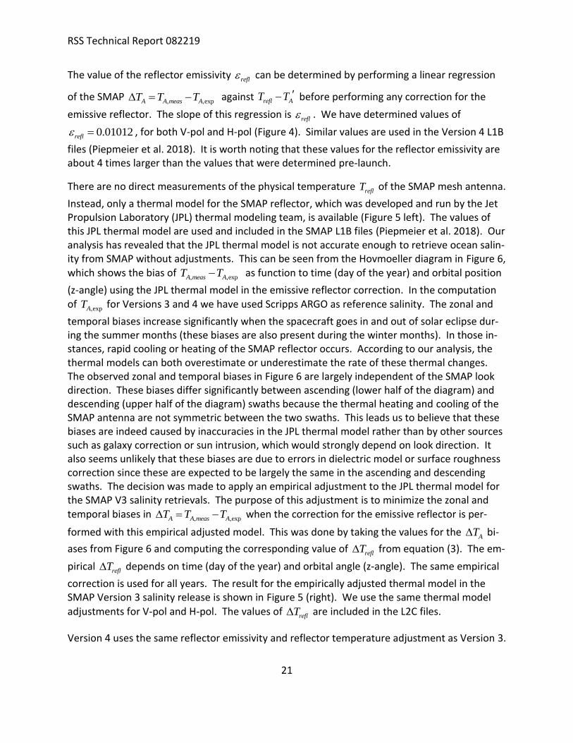
Figure 4: Regression of TA measured minus expected versus binned Trefl – TA. Trefl is the physical temperature of the antenna (from the JPL thermal model). TA is the radiometric antenna temperature. Blue: V-pol. Red: H-pol. The slope of the linear fits is the reflector emissivity. The bin population (not shown) is very small at the lower and up-per end of the x-axis interval, which causes the outliers.

Figure 5: Physical temperature Trefl of the reflector. Left: JPL thermal model that is used in the SMAP L1B files (Piepmeier et al. 2018). Right: Reflector temperature in the RSS SMAP Version 3 release after the empirical adjust-

ment refl

T has been added.


21

The value of the reflector emissivity refl can be determined by performing a linear regression

of the SMAP , ,expA A meas AT T T = − against refl AT T − before performing any correction for the

emissive reflector. The slope of this regression is refl . We have determined values of

0.01012refl = , for both V-pol and H-pol (Figure 4). Similar values are used in the Version 4 L1B

files (Piepmeier et al. 2018). It is worth noting that these values for the reflector emissivity are about 4 times larger than the values that were determined pre-launch.

There are no direct measurements of the physical temperature reflT of the SMAP mesh antenna.

Instead, only a thermal model for the SMAP reflector, which was developed and run by the Jet Propulsion Laboratory (JPL) thermal modeling team, is available (Figure 5 left). The values of this JPL thermal model are used and included in the SMAP L1B files (Piepmeier et al. 2018). Our analysis has revealed that the JPL thermal model is not accurate enough to retrieve ocean salin-ity from SMAP without adjustments. This can be seen from the Hovmoeller diagram in Figure 6, which shows the bias of

, ,expA meas AT T− as function to time (day of the year) and orbital position

(z-angle) using the JPL thermal model in the emissive reflector correction. In the computation of

,expAT for Versions 3 and 4 we have used Scripps ARGO as reference salinity. The zonal and

temporal biases increase significantly when the spacecraft goes in and out of solar eclipse dur-ing the summer months (these biases are also present during the winter months). In those in-stances, rapid cooling or heating of the SMAP reflector occurs. According to our analysis, the thermal models can both overestimate or underestimate the rate of these thermal changes. The observed zonal and temporal biases in Figure 6 are largely independent of the SMAP look direction. These biases differ significantly between ascending (lower half of the diagram) and descending (upper half of the diagram) swaths because the thermal heating and cooling of the SMAP antenna are not symmetric between the two swaths. This leads us to believe that these biases are indeed caused by inaccuracies in the JPL thermal model rather than by other sources such as galaxy correction or sun intrusion, which would strongly depend on look direction. It also seems unlikely that these biases are due to errors in dielectric model or surface roughness correction since these are expected to be largely the same in the ascending and descending swaths. The decision was made to apply an empirical adjustment to the JPL thermal model for the SMAP V3 salinity retrievals. The purpose of this adjustment is to minimize the zonal and temporal biases in

, ,expA A meas AT T T = − when the correction for the emissive reflector is per-

formed with this empirical adjusted model. This was done by taking the values for the AT bi-

ases from Figure 6 and computing the corresponding value of reflT from equation (3). The em-

pirical reflT depends on time (day of the year) and orbital angle (z-angle). The same empirical

correction is used for all years. The result for the empirically adjusted thermal model in the SMAP Version 3 salinity release is shown in Figure 5 (right). We use the same thermal model

adjustments for V-pol and H-pol. The values of reflT are included in the L2C files.

Version 4 uses the same reflector emissivity and reflector temperature adjustment as Version 3.


22

In our approach to empirically determine both refl and

reflT for SMAP, we have tried to avoid

folding potential errors in one quantity into the other. When determining the value of refl

from the linear regression (Figure 4), we only used cases where the JPL thermal model was de-termined to be accurate i.e., where the biases in Figure 6 are small (less than 0.1 K).

In the releases prior to Version 3, the HYCOM SSS field was used to derive reflT . This resulted

in significant temporal and zonal biases when compared to in-situ data. The main origin of these biases was the HYCOM field.

Figure 6: Hovmoeller diagram of SMAP TA measured - expected over the open ocean using the JPL thermal model for the SMAP mesh antenna. The x-axis is time (day of the year) and the y-axis is orbital position (z-angle). For the computation of TA expected we have used Scripps ARGO as reference salinity. The computation of this diagram is based on 2 years of SMAP data (September 2015 – August 2017). A simple spatial and temporal low-pass filter was applied by performing a running average in both dimensions.

4.4 Atmospheric Oxygen Absorption

The SMAP Version 2 release used the oxygen absorption model by Wentz and Meissner (2016). The SMAP Version 3 and Version 4 releases uses the oxygen absorption model by Liebe et al. (1992), as does the Aquarius Version 5 release.

4.5 IMERG Rain Rate and Correction for Liquid Cloud Water Absorption

The SMAP Version 2 salinity retrieval algorithm uses cloud water density profiles from NCEP GDAS. Analysis has shown that these NCEP cloud water profiles are unreliable and therefore cannot serve as a realistic source for a cloud water absorption correction in the salinity retrieval algorithm.


23

The IMERG rain product (Huffman et al. 2019), available from https://pps.gsfc.nasa.gov/, is a Level 4 merged product for surface rain rates, which is largely based on observations by NASA’s Global Precipitation Mission (GPM). It is currently regarded as the best available merged rain product by the scientific community. It is available for the whole SMAP operational period. We are using the Version 6 30-minute 0.1o product.

The IMERG rain rate RIMERG is resampled from its 0.1o spatial resolution to the 40-km SMAP res-olution. At each cell of the SMAP 0.25o fixed Earth grid, we compute an average IMERG rain rate by integrating over an approximate SMAP antenna gain. This approximate antenna gain is a circular Gaussian function with a half-power width of 40-km in both spatial dimensions. We then transform the resampled IMERG rain rate into columnar liquid cloud water content L fol-lowing the method by Hilburn and Wentz (2008). From L we compute the columnar absorption AL by liquid cloud water assuming Rayleigh approximation using the dielectric constant for pure (cloud) water by Meissner and Wentz (2004). With the updated value for AL from IMERG, we can then recompute the atmospheric parameters τ, TBUP, TBDW, that enter the atmospheric ab-sorption correction (Meissner et al. 2017, 2018).

The IMERG rain rate is also used for rain flagging in the ocean-target calibration (Section 4.8) and for producing the rain-flagged monthly Level 3 data (Section 7.2).

4.6 Correction for Reflected Galaxy

The correction for the reflected galaxy uses a combination of the geometric optics model for reflection from rough ocean surfaces and the results from the SMAP for – aft look analysis. It is described in detail in Meissner et al. 2017 and Meissner et al. 2018. The empirical zonal sym-metrization that was done in the Aquarius Version 5 release is not done for the SMAP Version 3.0 release.

4.7 Antenna Pattern Correction (APC)

Table 3: A-matrix elements Aij (in I, Q, S3, S4 basis) of the SMAP V3 release. The entries in red denote matrix ele-ments that differ from the pre-launch computation.

j=1 j=2 j=3 j=4

i=1 1.0929 -0.0001 0.0036 -0.0006

i=2 0.0000 1.1349 +0.0066 -0.0001

i=3 0.0009 0.0042 1.1336 -0.0553

i=4 0.0003 0.0014 +0.0117 1.1297

The matrix A transforms the Stokes vector of the Earth TA into TOI (top of the ionosphere) TB (Meissner et al. 2017):

B,TOA A,EarthT = A T (4)

https://pps.gsfc.nasa.gov/


24

The SMAP 4x 4 A-matrix elements are computed from SMAP pre-launch antenna patterns that have been created by the JPL antenna group from the GRASP software (file SMAP_An tenna_Pattern_verF_Freq1413_Ang000_2D.dat, provided by Emmanuel Dinnat, GSFC).

For the Version 3 and Version 4 releases, we have adjusted some of the A-matrix elements. These adjustments were done in order to:

1. Get the best TB over ocean scenes and the Amazon rainforest for all 4 Stokes parameters (I, Q, S3, S4).

2. Minimize spurious observed cross-talk dependencies between I, Q and S3, S4.

The A-matrix elements of the V3 and V4 salinity release are listed in Table 3.

The non-linear IU coupling that was observed in the Aquarius data (Meissner et al. 2017) is not observed with SMAP.

4.8 Ocean Target Calibration

The ocean target calibration (Meissner et al. 2017, 2018) removes any remaining, constant and time-varying biases in the TA measured – expected over the open ocean. We calculate the 3-

day running average of TA measured – expected ( ) ( ) ( ), ,expA A meas AT i T i T i = − as well as the

average ( )AT i for each orbit i over the open ocean for rain free scenes. The computation

of TA expected uses HYCOM as reference salinity. We require that the land fraction gland and the sea-ice fraction gice are both less than 0.0005, the IMERG rain rate is less than 0.1 mm/h (bit 15 in Table 4) and the flags for sun-glint (bit 5 in Table 4), moonglint (bit 6 in Table 4) and high reflected galaxy (bit 7 in Table 4) are not set.

The values of ( )AT i and ( )AT i are included in the metadata of the L2 files. We assume

that any remaining calibration adjustment is an effective adjustment of the noise-diode tem-

perature NDT . If

ApT is the antenna temperature of a SMAP observation for polarization p = V

or H after correcting for the emissive reflector, then we calculate the calibrated antenna tem-

perature ,Ap calT as:

( )

( )( ),

, ,A p

Ap cal Ap Ap D

Ap D

T iT T T T p V H

T i T

= − − =

− (5)

The DT in equation (5) stands for an average value of the Dicke load temperature. For our

purposes, we set this to a value of 293 K. Per construction, the running 3-day average of

,Ap calT is zero for each orbit: ( ), 0Ap calT i = .


25

We have also found small offsets for the S3 and S4, which are constant in time after the SMAP radar was shut off but differ during the time period before that. The following offset correction for S3 and S4 is performed:

, , 3, 4Ap cal Ap Ap offsetT T T p S S= − = (6)

The offset values ,Ap offsetT are +0.22 K (for S3) and -0.43 K (for S4) for the time after orbit #

2812. For the time before orbit # 2812, the offset values are 0.43 K (for S3) and -0.17 K (for S4).


26

5 SMAP SALINITY RETRIEVAL ALGORITHM: MAJOR UPDATES IN VERSION 4

5.1 Sidelobe Correction to Mitigate Land Intrusion

5.1.1 Computation of the SMAP Sidelobe Correction

The Aquarius and SMAP salinity retrievals degrade quickly as the footprint gets within 500km of land. This land-contamination error occurs because the land is radiometrically much warmer than the ocean. When the satellite observation gets close to land, a correction for land enter-ing the antenna sidelobes can be derived from simulated Aquarius and SMAP brightness tem-peratures (Meissner et al. 2017, 2018).

The land contamination is most conveniently dealt with at the TOA (top of the atmosphere). The error due to this contamination is given as:

, , , ,

ˆB TOA B TOA B TOA ml

T T T = − (7)

The 1st term on the right hand side of equation (7) is the simulated value of the actually ob-served (i.e. measured) signal. It is computed by simulating TOA Earth brightness temperatures containing representative ocean and land scenes and integrating them over the full SMAP an-tenna gain pattern. In the simulation, we use the pre-launch SMAP antenna pattern that was provided by the SMAP antenna group at JPL. The 2nd term of the right hand side of equation (7) is the true TOA TB coming from the antenna main beam. Using the simulated SMAP TB, a table

of the .B TOAT is computed one time off-line before the algorithm is run. In addition, the an-

tenna gain weighted land fraction gland is computed by integrating the antenna gain over the land covered area.

When computing the values for gland and ,B TOAT in the SMAP Version 2 release, it was assumed

that the position of the equatorial crossing repeats itself exactly every 8 days. This assumption is not accurate because there are small shifts in the equatorial crossing position from the target position. This has resulted in inaccuracies in the salinity retrievals near the coast after the land correction is applied.

Beginning with Version 3, the computation of gland and ,B TOAT no longer operates under this as-

sumption. Rather, we are keeping the equatorial crossing as a degree of freedom as was done in the Aquarius Version 5 land correction (Meissner et al. 2017; 2018). Because SMAP performs a full 360o scan, the sidelobe correction needs to be derived for a series of different scan posi-tions.

5.1.2 Major Changes in the Version 4 Sidelobe Correction

The spatial (latitude/longitude) resolution of the land tables has been increased to 0.125 o in Version 4.0 from 0.5 o in Version 3.0 (validated release) and 0.25 o in Version 3.3 (evaluation version). See Figure 7 for the effect of the spatial resolution of the land tables on the perfor-mance of the salinity retrieval algorithm near land.


27

Figure 7: SMAP – HYCOM salinity SSS, converted to ΔTB by multiplying with the sensitivity 𝑑𝑇𝐵

𝑑𝑆𝑆𝑆, as a function of

gland (antenna gain weighted land fraction). The x-axes are gland between 0 an 0.1 in increments of 0.01. The y-axes are ΔTB from -10 K to + 10 K in increments of 2 K. The value of sensitivity depends and SSS. Its computation is based on the dielectric model (Meissner and Wentz 2004, 2012). Upper: Using a 0.25o land correction table as in Version 3.3. There is overcorrection resulting in negative ΔTB. Lower: Using a 0.125 o land correction table as in Version 4.0. Note that the scatter at higher values of gland is also reduced with the Version 4.0 0.125 o land cor-rection. Also, note that the values of gland (x-axes) themselves change when increasing the resolution of the land correction tables.

The gland and TB,TOA land correction tables in SMAP Version 4.0 depend on:

1. Polarization (v-pol, h-pol). 2. Cell longitude (2880 elements in 0.125o increment). 3. Cell latitude (1441 elements in 0.125o increment). 4. Ascending/descending (2 elements). 5. Scan angle (30 elements in 12o increments). 6. The TB,TOA land correction tables also depend on time (12 months). The gland tables do not.

These variables result in the SMAP V4.0 TB,TOA land correction table having a dimensionality of (2, 2880,1441, 2, 30, 12).


28

The computation of the gland and TB,TOA land correction tables in SMAP Version 4.0 based on the orbit simulator follows the same basic procedure as in Aquarius Version 5 (Meissner et al. 2017, 2018).

5.1.3 Land Surface Emissivity

Figure 8: SMAP measured land TB minus land-emission model TB (based on NCEP soil moisture and land surface temperature).

For calculating the sidelobe correction near land it is necessary to know the TB that is emitted from the land surface. Up to and including Versions 3.0/3.3, we used a land surface emission model based on soil moisture and land surface temperature values from NCEP. In many coastal areas, the NCEP data for soil moisture are poor or non-existent. This resulted in significant er-rors in certain areas. Examples are the Aleutian Islands, the Gulf of Maine, and the Baja of Cali-fornia. The land emission in V4.0 is based on a 12-month climatology of SMAP TB over land.

SMAP measures TA over land in the coastal areas, which is contaminated by emission from the ocean through sidelobes. This contamination needs to be removed in order to obtain SMAP land surface TB. This can be used in the derivation of the land tables. The basic procedure is the same as removing the land contamination from an ocean observation near the coast. If the gain-weighted ocean fraction in the cell over land is gocean = 1 - gland , then the measured (ocean contaminated) TB is approximately given by:

( ), , ,1B meas ocean B land ocean B oceanT g T g T= − + (8)

The value of gocean = 1 - gland can be computed from the ocean simulator (section 5.1.1). The ocean TB has a much smaller dynamic range than the TB over land. We can therefore assume typical values for the TB,ocean (121 K for V-pol, 86 K for h-pol) in (8) and then solve (8) for TB,land in order to remove the ocean intrusion into the land scenes.


29

The difference between SMAP land TB and the NCEP based land model TB can reach 20 K in some areas (Figure 8).

5.1.4 Additional Empirical Corrections

Two additional empirical corrections are added in the sidelobe correction of the Version 4.0 re-lease. They are derived so that globally the TB measured minus expected curves become flat as function of gland.

1. A term that is proportional to 2 , which is the deviation of the spatial gradient of gland

from a strictly linear gradient.

1, 2

1

1, 2

150

160

B V pol

B

B H pol

TT

T

−

−

= =

(9)

The value of ( )2 ,i j at a grid point (i, j) of the 1/8o grid of the land correction tables is deter-

mined as:

( ) ( )2

1, 1,11, 1,1

1, ,

9land land

k i il j j

g k l g i j= − += − +

= −

(10)

If gland at the cell (i, j) is a strict linear function in 2-dimensional space, then 2 0 = . For the sim-

ple case of only 1 spatial dimension as degree of freedom, the value of 2 is characteristic for

the 2nd derivative of gland as function of spatial distance from the coast. When getting very close to the coast, the value of gland increases very rapidly as function of distance from the coast. That results generally in an over-correction error when doing a linear interpolation between the grid cells of the land correction tables. The size of this error depends on the spatial resolution of the land correction tables. In V3, where the spatial resolution of the land table was only ½o, this caused a large error close to the coast, which made the land correction basically useless. Even in V4, where the spatial resolution of the land correction is 1/8o a residual error remains. The purpose of the correction (9) is to compensate for this error.

2. An empirical term that increases linearly with gland above 0.02.

( )

( )2,

2

2,

78 0.02, 0.02

83 0.02

B V pol land

B land

B H pol land

T gT g

T g

−

−

− = =

− (11)

If gland < 0.02 the 2BT is set to 0. At gland = 0.04, which is the largest value for land contamina-

tion that is regarded to give a useful salinity retrieval, the size of 2BT is about 25% of the size

of the sidelobe correction.


30

5.1.5 Land Exclusion for Calculating Smoothed Product

If the SMAP 3-dB footprint actually touches land, the sidelobe correction breaks down. In V4.0 we introduce an additional land contamination fraction, called fland, which is the percentage of land within the 3-dB footprint. This parameter is used for screening and flagging in addition to the gain weighted fraction gland. This becomes particularly important close to the many small islands in the Central Pacific.

The smoothed product sss_smap is obtained from the 40-km product sss_smap_40km by com-puting the next-neighbor average at each 0.25o grid cell. See section 2.7 equation (1). The next-neighbor average normally consists of the center cell plus 8 adjacent cells, but cells are excluded in the case of land contamination. Cells are excluded for land contamination if one of the following conditions apply:

1. The value of gland > 0.04.

2. The value of fland > 0.001.

If either of these conditions is true for a given cell, then it is not used in the next-neighbor aver-age. The values of gland and fland are based on averages over all possible look angles in each Earth grid cell.

5.1.6 Results and Performance of Land Correction in Version 4.0

Figure 9: SMAP – HYCOM salinity near Baja California (May 2018). Left: Version 3.0 70-km product. A large area near the coast was flagged for land contamination. Center: V3.3 70-km product. Right Version 4.0 smoothed product.

Figure 9 shows monthly maps (05/2018) of SMAP – HYCOM SSS near the Baja of California for the V3.0, V3.3, and V4.0 70-km/smoothed products. In V3.0 areas within more than 100-km from the coast were flagged to avoid land contamination. Nevertheless, light land contamina-tion is still visible near some coastal areas. In V3.3 the threshold for land contamination was increased, which resulted in strongly contaminated cells near the coast. In V4.0 we can retrieve


31

SSS within 30 – 40 km from land. Other examples of the improvement in the land correction in V4.0 are shown in Figure 10, Figure 11 and Figure 12.

Figure 10: Statistics of RSS SMAP L2C versus ARGO match-ups as a function of gland. Left: V3.3. Right: V4.0. Me-dian (white curve) and standard deviation (red curve). The colored shades indicate the 2-dimensional probability density. The analysis and figure were provided by H.-Y. Kao, ESR.

Figure 11: Improvement of land correction in V4.0 in Gulf of Maine area. The plots show comparison between SMAP and 3 moored buoys. The salty bias in SMAP V3 (blue) compared to Buoy M01 (black), which is close to the coast, is strongly reduced in V4 (red). The analysis and figure were provided by S. Grodsky, University of Maryland.


32

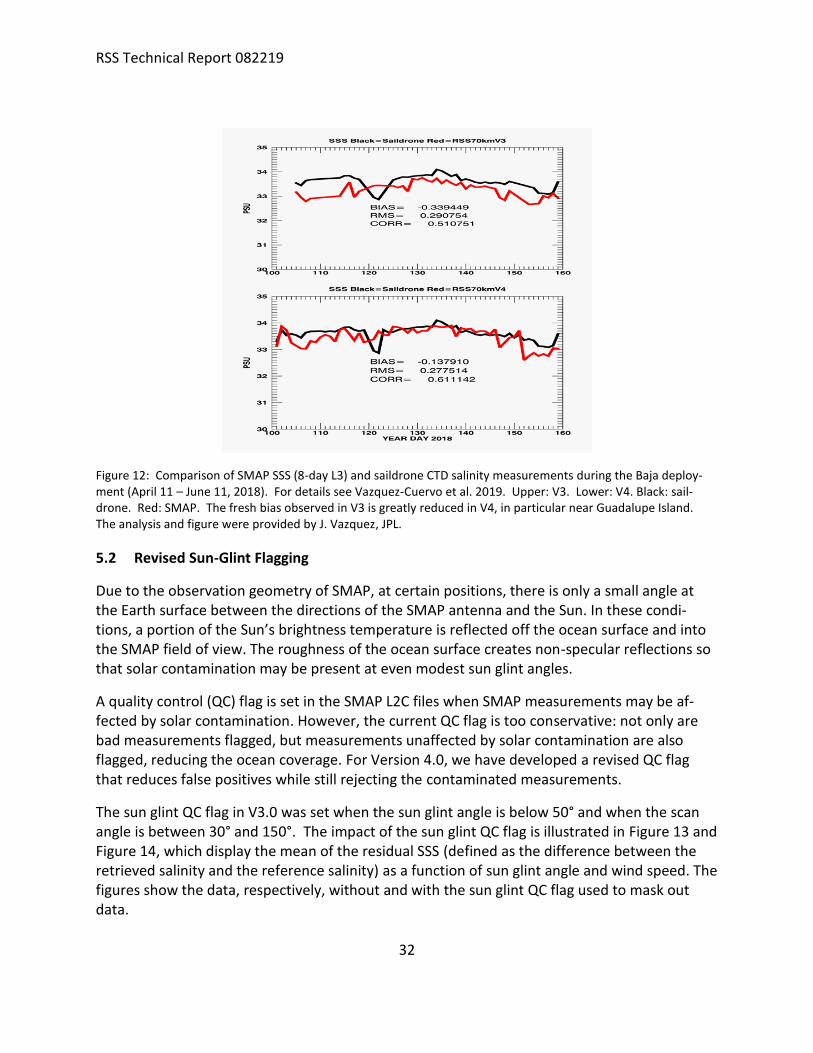
Figure 12: Comparison of SMAP SSS (8-day L3) and saildrone CTD salinity measurements during the Baja deploy-ment (April 11 – June 11, 2018). For details see Vazquez-Cuervo et al. 2019. Upper: V3. Lower: V4. Black: sail-drone. Red: SMAP. The fresh bias observed in V3 is greatly reduced in V4, in particular near Guadalupe Island. The analysis and figure were provided by J. Vazquez, JPL.

5.2 Revised Sun-Glint Flagging

Due to the observation geometry of SMAP, at certain positions, there is only a small angle at the Earth surface between the directions of the SMAP antenna and the Sun. In these condi-tions, a portion of the Sun’s brightness temperature is reflected off the ocean surface and into the SMAP field of view. The roughness of the ocean surface creates non-specular reflections so that solar contamination may be present at even modest sun glint angles.

A quality control (QC) flag is set in the SMAP L2C files when SMAP measurements may be af-fected by solar contamination. However, the current QC flag is too conservative: not only are bad measurements flagged, but measurements unaffected by solar contamination are also flagged, reducing the ocean coverage. For Version 4.0, we have developed a revised QC flag that reduces false positives while still rejecting the contaminated measurements.

The sun glint QC flag in V3.0 was set when the sun glint angle is below 50° and when the scan angle is between 30° and 150°. The impact of the sun glint QC flag is illustrated in Figure 13 and Figure 14, which display the mean of the residual SSS (defined as the difference between the retrieved salinity and the reference salinity) as a function of sun glint angle and wind speed. The figures show the data, respectively, without and with the sun glint QC flag used to mask out data.


33

While effective at removing the contaminated measurements, many un-contaminated meas-urements are also removed by the flag, especially at low winds. Furthermore, a discontinuity is present at the sun glint angle = 50° line, since a few measurements are present below that an-gle yet are outside the scan angle range of 30° to 150°.

Figure 13: The mean of the residual SSS as a function of sun glint angle and wind speed. Large magnitude errors are clamped for display purposes. The grey shaded area contains no data.

For Version 4, we define a revised sun glint flag that is a function of both the sun glint angle as well as the wind speed (but not a function of scan angle). The QC flag is set if the sun glint angle is below 50°, and if the wind speed 𝑤 exceeds a threshold, which is a parameter of sun glint an-gle 𝑔:

41( 30 )

8000w g − (12)

With this revised sun glint QC flag applied, the mean of the residual SSS is shown in Figure 15. The discontinuity at the 50° line is removed and no large bias from solar contamination is pre-sent.

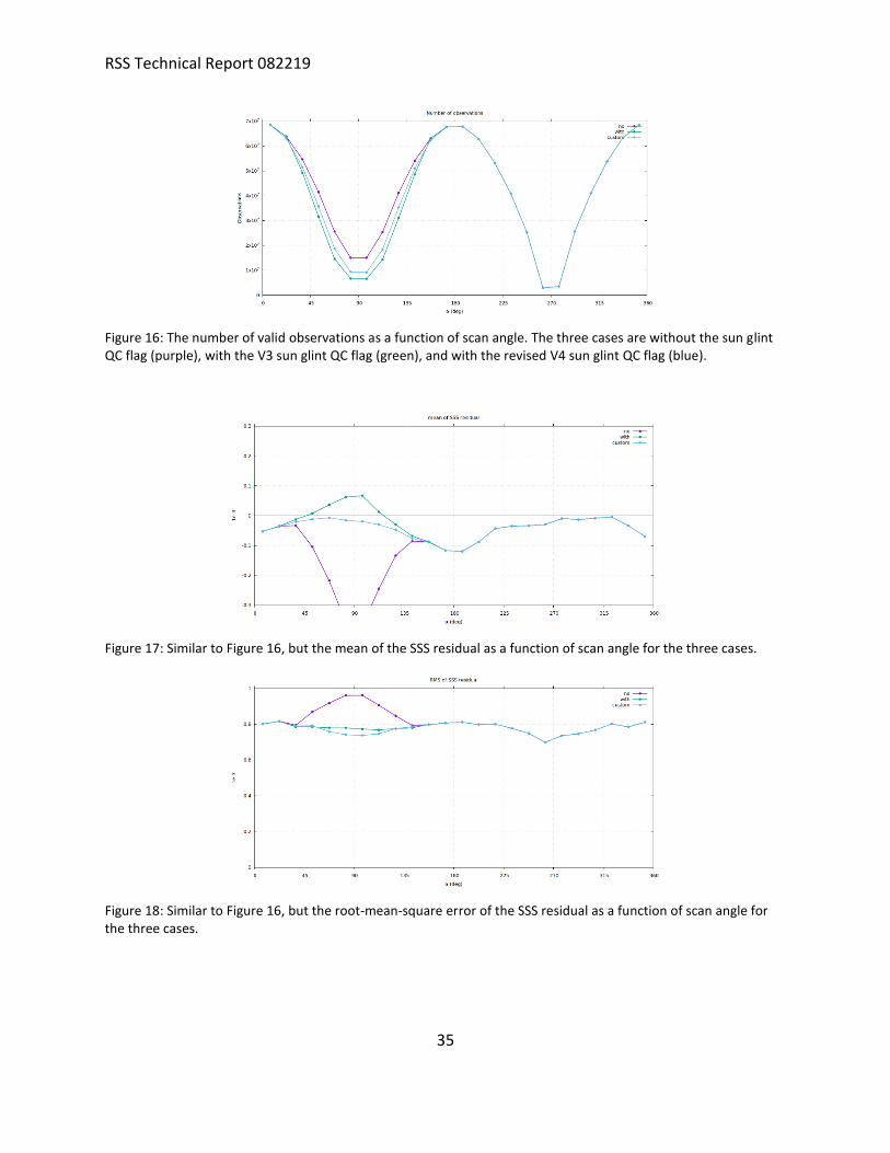
With the revised sun glint QC flag, the number of valid observations retained is larger than with the previous version of the flag (Figure 16). The mean of the SSS residual is shown in Figure 17 and the root-mean-square (RMS) error is shown in Figure 18. These show that although the number of SMAP measurements retained increases with the revised sun glint QC flag, the error


34

in the additional measurements is similar to non-contaminated cases. This indicates that there is no significant solar contamination in additional measurements.

Figure 14: As Figure 13, but the V3 sun glint QC flag is used to mask out data.

Figure 15: As Figure 13, but with the revised sun glint QC flag for V4.


35

Figure 16: The number of valid observations as a function of scan angle. The three cases are without the sun glint QC flag (purple), with the V3 sun glint QC flag (green), and with the revised V4 sun glint QC flag (blue).

Figure 17: Similar to Figure 16, but the mean of the SSS residual as a function of scan angle for the three cases.

Figure 18: Similar to Figure 16, but the root-mean-square error of the SSS residual as a function of scan angle for the three cases.


36

5.3 Revised Sea-Ice Mask and Flagging

For the NASA/RSS Aquarius salinity retrieval up to Version 4 and the RSS SMAP salinity retrieval up to and including Version 3, the daily sea-ice mask from NCEP was used as ancillary field. Brucker et al. 2014 and Dinnat and Brucker (2016) found that the NCEP sea-ice mask is unrealis-tic in several instances. Consequently, for the Aquarius Version 5 end of mission release, a sea-ice mask from SSMI and AMSR-2 was implemented instead of the NCEP sea-ice mask.

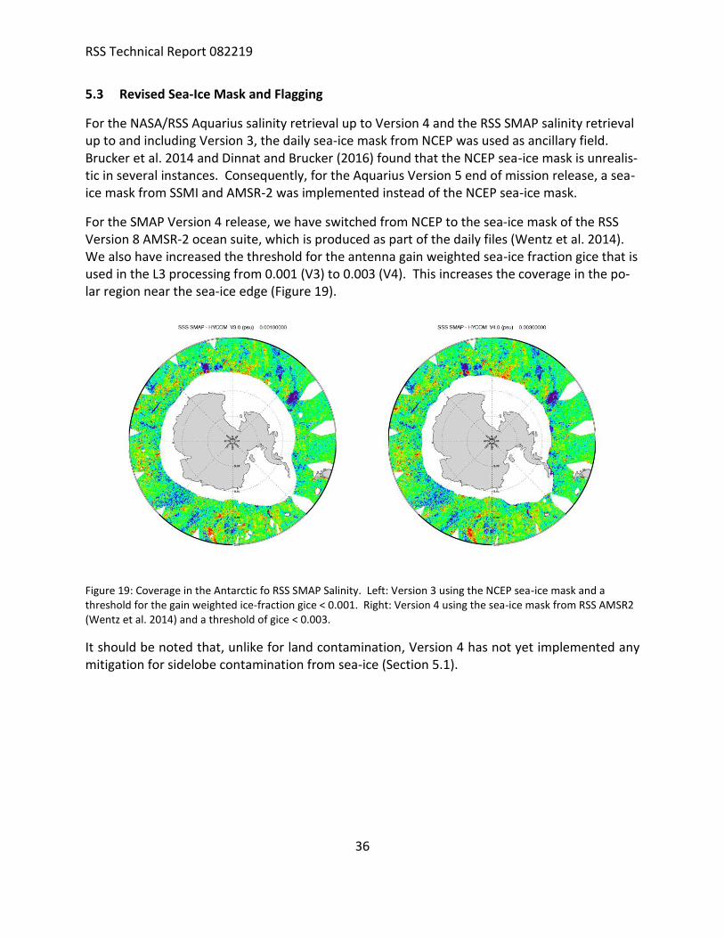
For the SMAP Version 4 release, we have switched from NCEP to the sea-ice mask of the RSS Version 8 AMSR-2 ocean suite, which is produced as part of the daily files (Wentz et al. 2014). We also have increased the threshold for the antenna gain weighted sea-ice fraction gice that is used in the L3 processing from 0.001 (V3) to 0.003 (V4). This increases the coverage in the po-lar region near the sea-ice edge (Figure 19).

Figure 19: Coverage in the Antarctic fo RSS SMAP Salinity. Left: Version 3 using the NCEP sea-ice mask and a threshold for the gain weighted ice-fraction gice < 0.001. Right: Version 4 using the sea-ice mask from RSS AMSR2 (Wentz et al. 2014) and a threshold of gice < 0.003.

It should be noted that, unlike for land contamination, Version 4 has not yet implemented any mitigation for sidelobe contamination from sea-ice (Section 5.1).


37

6 QUALITY CONTROL (Q/C) FLAGS

The V4.0 salinity retrieval algorithm produces the following Q/C flags:

Table 4: 32- bit Level 2 Q/C flags in the SMAP V4.0 release.

bit Q/C flag if bit is set SSS value and expected level of degradation

0 no valid radiometer observation in cell SSS value set to missing/invalid

1 problem with OI: parameter wt_sum not normalized to 1

SSS value set to missing/invalid

2 strong land contamination: gain weighted land fraction gland exceeds 0.1 or land fraction in 3-dB footprint fland exceeds 0.1


3 strong sea ice contamination: gain weighted sea-ice fraction gice exceeds 0.1 or sea-ice fraction in 3-dB footprint fice exceeds 0.1


4 MLE in SSS retrieval algo has not converged: iflag_sss_conv = 1


5 sunglint: see Section 5.2

SSS retrieved very strong degradation not included in averaging for the 70-km smoothed product

6 moonglint: moonglint angle monglt less than 15°

SSS retrieved moderate – strong degradation not included in averaging for the 70-km smoothed product

7 high reflected galaxy: 1st component ta_gal_ref(1, …)/2 [=(V+H)/2] ex-ceeds 2.0K.


8 moderate land contamination: gain weighted land fraction gland exceeds 0.04 or land fraction in 3-dB footprint fland exceeds 0.001

SSS retrieved moderate -strong degradation not included in averaging for the 70-km smoothed product

9 moderate sea ice contamination: gain weighted sea ice fraction gice exceeds 0.003


10 high residual of MLE in SSS retrieval algo: Variable tb_consistency exceeds 1.0 K.


11 low SST: surtep - 273.15 below 5°C

SSS retrieved moderate – strong degradation

12 high wind speed: winspd exceeds 15 m/s

SSS retrieved moderate degradation

13 light land contamination gain weighted land fraction gland exceeds 0.001

SSS retrieved light degradation

14 light sea-ice contamination gain weighted sea-ice fraction gice exceeds 0.001

SSS retrieved light degradation


38

15 rain flag: IMERG rain-rate (resampled to 40-km SMAP foot-print) exceeds 0.1 mm/h.

SSS retrieved possible light degradation due to degraded wind speed or poor atmospheric correction. Validation of SMAP versus ARGO/HYCOM might result in error due to SSS stratification within the upper ocean layer

16 - 31 sparse


39

7 LEVEL 3 PROCESSING

7.1 Standard Product

Both the 40-km (sss_smap_40km) and the sss_smap (smoothed to approximately 70km) L2C salinity products are averaged into Level 3 data product. The L3 grids are regular 0.25o lati-tude/longitude Earth grids created by averaging all valid L2C observations within each grid cell, as described in the following. First, for and aft looks are averaged together. Then, we produce a running 8-day average L3 and a monthly average L3 file. For an 8-day running average that is centered on a given day of the year (DOY) we average all valid observations within +/- 3.5 days of said DOY. For example, the L3 file for January 15 is created by averaging L2 observations that fall between 12UTC January 11 and 12UTC January 19. The reason for providing 8-day averages rather than weekly averages is that SMAP has an exact 8-day repeat cycle. For the monthly av-erage files, we average all valid data within the corresponding calendar month. The L3 pro-cessing performs only time averaging of the L2C data. No additional spatial smoothing of the L2C data is done in the L3 processing.

During the gridding for both the 8-day running averages and the monthly averages, we apply Q/C checks and discard data if:

1. The sun glint flag (bit 5 in L2 Q/C flag Table 4) is set. 2. The moon glint angle is less than 15o (bit 6 in L2 Q/C flag Table 4 is set). 3. The v/h-pol average of the reflected galactic radiation exceeds 2.0 K (bit 7 in L2 Q/C flag Ta-

ble 4 is set).

4. The TB consistency, which is defined as the 2 of the MLE in the salinity retrieval algo-

rithm, exceeds 1.0 K (bit 10 in L2 Q/C flag Table 4 is set). 5. The gain weighted land fraction gland exceeds 0.04 or the land fraction in the 3-dB footprint

fland exceeds 0.001 (bit 8 in L2 Q/C flag Table 4 is set). 6. The gain weighted sea ice fraction gice exceeds 0.003 (bit 9 in L2 Q/C flag Table 4 is set). 7. The wind speed exceeds 20 m/s.

The L3 files contain the number of observations in each grid cell as well as averaged values of salinity, gland, fland, gice, and the ancillary SST in each grid cell.

Browsing images for both 8-day and monthly averages are available on the RSS website (http://www.remss.com/missions/smap/).

7.2 Rain Filtered (RF) Product

Starting with Version 3 we also produce a rain-filtered (RF) monthly L3 product. In doing so, we discard data if the IMERG rain rate (Section 4.5), resampled to 40km, exceeds 0.1 mm/h (bit 15 in Table 4 is set). This RF product also includes the Scripps ARGO analyzed salinity field to allow easy comparison with the SMAP retrievals. Note that the Scripps ARGO field is not used any-where in the L2 or L3 processing but is only included for comparison in the RF product. Because of the latency of the Scripps ARGO field (a couple of months), the latency of the L3 RF monthly



40

product is larger than that of the standard monthly L3 product. The RF monthly product is only distributed on the RSS website and is not available from PO.DAAC.

7.3 Empirical Uncertainty Estimate

In the Version 4.0 L3 files (8-day running, monthly, monthly_RF), we provide an empirical un-certainty estimate for the standard/default product sss_smap that has been smoothed to ap-proximately 70km. This empirical uncertainty estimate is based on comparisons between the sss_smap and the analyzed Scripps ARGO salinity field. The uncertainty estimate is the root-mean square (RMS) difference between SMAP and ARGO and contains both random and sys-tematic uncertainties. Note that it also includes the sampling error of the Argo data on the scales of the gridded maps, as well as the mapping errors (Lee 2016). Because of the different noise reduction in the different time averages (8-day running, monthly), the uncertainty esti-mates between 8-day running and monthly fields differ.

We assume that the major drivers for the L3 uncertainties are:

1. SST and SSS: They drive the sensitivity of the measured TB to SSS.

2. Degree of land contamination measured by gland.

For the uncertainty estimate, we have run an off-line comparison between the sss_smap in the RSS L3 files and the ARGO field for 4 years of data. The results are binned and tabulated with respect to gland. We transform the salinity uncertainty estimate ∆S into a ΔTB uncertainty esti-mate by multiplying the ∆S with the computed sensitivity:

( ),

,

,B V pol S

B est est

comp

T T ST S

S

− =

(13).

The result is a look-up table ∆TB as a function of gland. The reason for tabulating ∆TB rather than ΔS is that the salinity uncertainty as a function of gland changes with SST. It is larger in

cold SST as the sensitivity to SSS decreases in cold water. The sensitivity ( ), ,B V pol S

comp

T T S

S

−

is

computed from the dielectric constant model (Meissner and Wentz, 2004, 2012).

During the L3 processing, the uncertainty estimate for sss_smap can then be obtained from this

∆TB look-up table by dividing by the sensitivity ( ), ,B V pol S

comp

T T S

S

−

, which is computed at each

L3 grid cell from the L3 values of SST and SSS.


41

8 OPEN OCEAN PERFORMANCE ESTIMATE AND VALIDATION

This section shows validation results for SMAP V3 over the open ocean (gland < 0.001). Be-cause the salinity retrieval over the open ocean is basically unchanged in V4 from V3, the re-sults presented in this section apply also to V4.

8.1 Spatial Resolution and Noise Figures

When comparing V3.0 or V4.0 SMAP SSS with the HYCOM SSS field, we find that the SMAP Level 2C SSS at a 40-km resolution has an estimated accuracy of about 0.9 psu due to the high noise figures of the L1B TA, which is input into the L2 processing.

When comparing the V3.0 SMAP Level 2C SSS at a 70-km resolution or the V4.0 Level 2C SSS (sss_smap, which has been smoothed to approximately 70km) to the HYCOM SSS field, we con-clude that this product has an estimated accuracy of about 0.5 psu due to the reduction in noise caused by the spatial smoothing of the L1B TA.

8.2 Time Series of SMAP – ARGO – HYCOM Comparisons over the Open Ocean

Figure 20: Time series (APR 2015 – JUN 2018) of biases (∆SSS): SMAP V3 – HYCOM (blue). SMAP V3 – Scripps ARGO (red). Scripps ARGO – HYCOM (dashed black). The figure was created from the Level 3 70-km rain-filtered monthly maps requiring gland < 0.001, gice < 0.001, SST>5◦C. The x-axis increments are months since the start of the mission.

Time series of biases and standard deviations between SMAP V3, Scripps ARGO and HYCOM for monthly rain-filtered averages are shown in Figure 20 - Figure 23. Assuming that the errors in the 3 data sets are uncorrelated, the RMS in the SMAP product can be estimated from the triple collocation method:


42

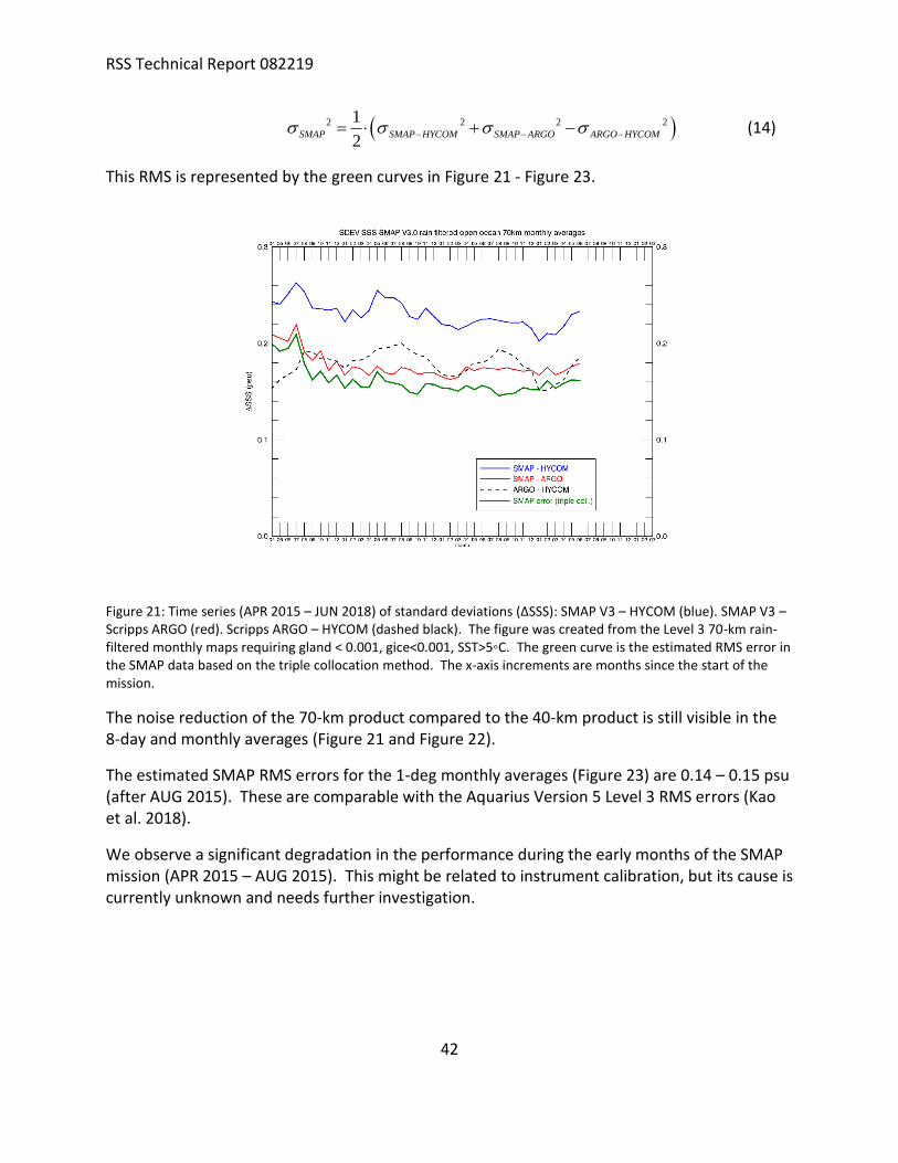
( )2 2 2 21

2SMAP SMAP HYCOM SMAP ARGO ARGO HYCOM − − −= + − (14)

This RMS is represented by the green curves in Figure 21 - Figure 23.

Figure 21: Time series (APR 2015 – JUN 2018) of standard deviations (∆SSS): SMAP V3 – HYCOM (blue). SMAP V3 – Scripps ARGO (red). Scripps ARGO – HYCOM (dashed black). The figure was created from the Level 3 70-km rain-filtered monthly maps requiring gland < 0.001, gice<0.001, SST>5◦C. The green curve is the estimated RMS error in the SMAP data based on the triple collocation method. The x-axis increments are months since the start of the mission.

The noise reduction of the 70-km product compared to the 40-km product is still visible in the 8-day and monthly averages (Figure 21 and Figure 22).

The estimated SMAP RMS errors for the 1-deg monthly averages (Figure 23) are 0.14 – 0.15 psu (after AUG 2015). These are comparable with the Aquarius Version 5 Level 3 RMS errors (Kao et al. 2018).

We observe a significant degradation in the performance during the early months of the SMAP mission (APR 2015 – AUG 2015). This might be related to instrument calibration, but its cause is currently unknown and needs further investigation.


43

Figure 22: Same as Figure 21 for the 40-km product.

Figure 23: Same as Figure 21 for 1-deg lat/lon averages.


44

8.3 Zonal and Average Regional Biases

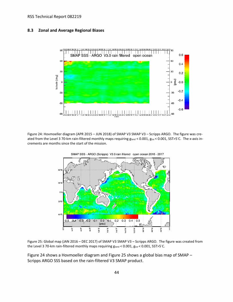
Figure 24: Hovmoeller diagram (APR 2015 – JUN 2018) of SMAP V3 SMAP V3 – Scripps ARGO. The figure was cre-ated from the Level 3 70-km rain-filtered monthly maps requiring gland < 0.001, gice < 0.001, SST>5◦C. The x-axis in-crements are months since the start of the mission.

Figure 25: Global map (JAN 2016 – DEC 2017) of SMAP V3 SMAP V3 – Scripps ARGO. The figure was created from the Level 3 70-km rain-filtered monthly maps requiring gland < 0.001, gice < 0.001, SST>5◦C.

Figure 24 shows a Hovmoeller diagram and Figure 25 shows a global bias map of SMAP – Scripps ARGO SSS based on the rain-filtered V3 SMAP product.


45

The V2 SMAP release had significant salty biases at low latitudes and fresh biases at high lati-tudes in the SMAP SSS. These biases have been greatly reduced in the V3 release.


46

9 REFERENCES

Atlas, R., R. N. Hoffman, J. Ardizzone, S. M. Leidner, J. C. Jusem, D. K. Smith, D. Gombos, 2011: A cross-calibrated, multiplatform ocean surface wind velocity product for meteorological and oceanographic applications. Bull. Amer. Meteor. Soc., 92, 157-174. doi: 10.1175/2010BAMS2946.1

Brucker, L., E. Dinnat, and L. Koenig, 2014, Weekly gridded Aquarius L-band radiometer/scatterometer observa-tions and salinity retrievals over the polar regions-Part 2: Initial product analysis, Cryosphere, 8(3), 915–930, doi:10.5194/tc-8-915-2014.

Dinnat, E. and L. Brucker, 2016, Improved Sea Ice Fraction Characterization for L-Band Observations by the Aquar-ius Radiometers, IEEE Transactions on Geoscience and Remote Sensing, doi:10.1109/TGRS.2016.2622011.

Hilburn, K. and F. Wentz, 2008, Intercalibrated passive microwave rain products from the unified microwave ocean retrieval algorithm (UMORA), Journal of Applied Meteorology and Climatology, 47, 778-794.

Huffman, G. et al., 2019, NASA Global Precipitation Measurement (GPM) Integrated Multi-satellitE Retrievals for GPM (IMERG), Version 6, NASA, Available online at https://pmm.nasa.gov/sites/default/files/document_files/ IMERG_V06_release_notes_190503.pdf.

Kao, H.-Y., G. Lagerloef, T. Lee, O. Melnichenko, T. Meissner and P. Hacker, 2018, Assessment of Aquarius Sea Sur-face Salinity, Remote Sens. 10(9), https://doi.org/10.3390/rs10091341.

Lee, T., 2016, Consistency of Aquarius sea surface salinity with Argo products on various spatial and temporal scales, Geophys. Res. Lett., vol. 43(8), pp 3857-3864, https://doi.org/10.1002/2016GL068822.

Liebe, H., P. Rosenkranz and G. Hufford, 1992, Atmospheric 60-GHz oxygen spectrum: New laboratory measure-ments and line parameters, J. Quant. Spectrosc. Radiat. Transfer, 48, 629–643, doi: 10.1016/0022-4073(92)90127-P.

Mears, C. et al. 2018: Remote Sensing Systems Cross-Calibrated Multi-Platform (CCMP) 6-hourly ocean vector wind analysis product on 0.25 deg grid, Version 2.0. Remote Sensing Systems, Santa Rosa, CA. Available online at www.remss.com/measurements/ccmp.

Meissner, T., and F. Wentz, 2004, The complex dielectric constant of pure and sea water from micro-wave satellite observations, IEEE TGRS, vol. 42(9), pp 1836.

Meissner, T. and F. Wentz, 2012, The emissivity of the ocean surface between 6 and 90 GHz over a large range of wind speeds and Earth incidence angles, IEEE TGRS, 2012, 50(8), 3004–3026, doi: 10.1109/TGRS.2011.2179662.

Meissner, T., F. Wentz, and L. Ricciardulli, 2014: The emission and scattering of L-band microwave radiation from rough ocean surfaces and wind speed measurements from Aquarius, J. Geophys. Res. Oceans, vol. 119, doi: 10.1002/2014JC009837.

Meissner, T., F. Wentz F. and D. M. Le Vine, 2017, Aquarius Salinity Retrieval Algorithm Theoretical Basis Document (ATBD), End of Mission Version; RSS Technical Report 120117; 1 December 1 2017. Available online at ftp://po-daac-ftp.jpl.nasa.gov/allData/aquarius/docs/v5/AQ-014-PS-0017_Aquarius_ATBD-EndOfMission.pdf.

Meissner, T, F.J. Wentz, and D.M. Le Vine, 2018, The Salinity Retrieval Algorithms for the NASA Aquarius Version 5 and SMAP Version 3 Releases, Remote Sensing 10, 1121, doi:10.3390/rs10071121.

Piepmeier, J. et al., 2014: SMAP Calibrated, Time-Ordered Brightness Temperatures L1B_TB Data Product, Algo-rithm Theoretical Basis Document (ATBD), https://smap.jpl.nasa.gov/documents/.

https://doi.org/10.3390/rs10091341

https://doi.org/10.1002/2016GL068822

http://www.remss.com/measurements/ccmp

ftp://podaac-ftp.jpl.nasa.gov/allData/aquarius/docs/v5/AQ-014-PS-0017_Aquarius_ATBD-EndOfMission.pdf

ftp://podaac-ftp.jpl.nasa.gov/allData/aquarius/docs/v5/AQ-014-PS-0017_Aquarius_ATBD-EndOfMission.pdf

https://smap.jpl.nasa.gov/documents/


47

Piepmeier, J. et al. 2018: SMAP L1B Radiometer Half-Orbit Time-Ordered Brightness Temperatures, Version 4. [RFI filtered antenna temperatures]. Boulder, Colorado USA. NASA National Snow and Ice Data Center Distributed Ac-tive Archive Center. https://doi.org/10.5067/VA6W2M0JTK2N.

Poe, G., 1990, Optimum interpolation of imaging microwave radiometer data, IEEE Trans. Geosci. Remote Sens., vol. 28, no. 5, pp. 800-810.

Stogryn, A., 1978, Estimates of brightness temperatures from scanning radiometer data, IEEE Trans. Antennas Propag. vol. AP-26, no. 5, pp. 720 – 726.

Vazquez-Cuervo, J. et al., 2019, Using Saildrones to Validate Satellite-Derived Sea Surface Salinity and Sea Surface Temperature along the California/Baja Coast, Remote Sensing, https://doi.org/10.3390/rs11171964.

Wentz et al., 2014, Remote Sensing Systems GCOM-W1 AMSR2 Daily Environmental Suite on 0.25 deg grid, Version 8, Available from www.remss.com/amsr/.

Wentz, F., and T. Meissner, 2016: Atmospheric absorption model for dry air and water vapor at microwave fre-quencies below 100GHz derived from spaceborne radiometer observations, Radio Science, vol. 51, doi:10.1002/2015RS005858.

https://doi.org/10.5067/VA6W2M0JTK2N

https://doi.org/10.3390/rs11171964

http://www.remss.com/amsr/


48

10 DATA FORMAT SPECIFICATION

10.1 Level 2C

10.1.1 Paths and Filenames

• Pathname: /smap/SSS/V04.0/FINAL/L2C/yyyy/mm/... yyyy = 4-digit year, mm = 2-digit month.

• Filename: RSS_SMAP_SSS_L2C_rnnnnn_yyyymmddThhmiss_yyyyddd_FNL_V04.0.nc. nnnnn = 5-digit orbit (rev) #, yyyy = 4-digit year, mm = 2-digit month, dd = 2-digit day of month, hh=2-digit hour of day (UTC), mi = 2-digit minute of hour (UTC), ss = 2-digit second of minute (UTC), doy 3-digit day of year. The time stamp refers to the start time of the orbit.

10.1.2 Global Attributes

• orbit_number (4-byte integer): orbit (rev) #.

• start_time_sec2000 (8-byte real): seconds of first valid record in this rev since 2000-01-01 00:00:00 UTC.

• start_time_year, start_time_month, start_time_day_of_month, start_time_day_year (4-byte integer): year, month, day of month, day of year of first valid record in this rev.

• start_time_sec_of_day (8-byte real): seconds of day of first valid record in this rev.

• end_time_sec2000 (8-byte real): seconds of last valid record in this rev since 2000-01-01 00:00:00 UTC.

• end_time_year, end_time_month, end_time_day_of_month, end_time_day_year (4-byte integer): year, month, day of month, day of year of last valid record in this rev.

• end_time_sec_of_day (8-byte real): seconds of day of last valid record in this rev.

• emissivity_reflector_vpol, emissivity_reflector_hpol (4-byte real): ant (Section 4.3).

• A_ij (4-byte real): APC matrix element (i, j) where the indices i, j run over the Stokes vector I, Q, S3, S4 (Section 4.7).

• ta_ocean_ave_vpol, ta_ocean_ave_hpol (4-byte real): average ta over open ocean for this rev (Section 4.8).

• ta_bias_ocean_vpol, ta_bias_ocean_hpol, ta_bias_ocean_S3, ta_bias_ocean_S4 (4-byte real): TA biases= TA measured – expected over the open ocean (Section 4.8). The computation of TA expected is based on the HY-COM reference SSS. The computation of TA expected for the 3rd Stokes parameter (S3) is based on ancillary TEC maps from IGS (Table 2).

10.1.3 Gridding and Dimensions

The L2C files contain SMAP observations that were optimum interpolated onto a fixed 0.25o x 0.25o Earth grid.

The grid (x, y) dimensions are:

• xdim_grid=1560, which corresponds to 360o longitude plus 30o in order to accommodate the whole swath.


49

• ydim_grid =720, which corresponds to 180o latitude.

Though the grid cell indices are related to longitude and latitude, the variables cellon and cellat (Section 10.1.4) should be used to identify the location.

• look = 2 (1 = for look, 2= aft look) defines the look direction of the variable. If the variable does not depend on look direction, then this dimension is omitted.

• polarization_2 = 2, polarization_3 = 3, polarization_4 = 4 specifies the polarization of the variable fields. Note that for some variables the Stokes polarization basis (I, Q, S3, S4) is used, whereas for other variables the mod-ified Stokes polarization basis (V, H, S3, S4) is used. See Section 10.1.4.

Any grid cell for with one of the bits 0 – 1 set has invalid entries and none of the variable fields should be used. Any grid cells with one of the bits 2 – 3 set has no valid salinity retrieval.

10.1.4 Variables

All variable values refer to the average of the OI in the grid cell.

• time (8-byte float, array size = [look, xdim_grid, ydim_grid]): seconds of observation since 2000-01-01 00:00:00 UTC.

• cellat (4-byte float, array size = [look, xdim_grid, ydim_grid]): geodetic latitude. range: [90oS, 90oN].

• cellon (4-byte float, array size = [look, xdim_grid, ydim_grid]): longitude. range: [0o, 360o].

• eia (4-byte float, array size = [look, xdim_grid, ydim_grid]): boresight Earth incidence angle. range: [0o, 90o]

• eaa (4-byte float, array size = [look, xdim_grid, ydim_grid]): boresight Earth azimuth angle. range: [0o, 360o].

• zang (4-byte float, array size = [look, xdim_grid, ydim_grid]): orbital position angle of S/C. range: [0o, 360o]. It

is defined as: ( )

( )/

/

ˆ ˆarctan 90

ˆ ˆ

S C

S C

R zzang

V z

= +

. z is the z-unit vector in the Earth centered inertial system (ECI).

/ˆ

S CR is the S/C location unit vector in the ECI system. /

ˆS CV is the S/C velocity unit vector in the ECI system. 0o

is S, 90o is equator crossing in the ascending swath, 180o is N, 270o is equator crossing in the descending swath, 360o is S.

• alpha (4-byte float, array size = [look, xdim_grid, ydim_grid]): scan angle. range: [0o, 360o]. 0o is forward, 90o is left of forward, 180o is aft, 270o is right of forward, 360o is forward.

• pra (4-byte float, array size = [look, xdim_grid, ydim_grid]): polarization basis rotation angle (geometrical part), which is the angle between polarization basis of S/C and polarization basis on the Earth. range: [-90o, +90o].

• sunglt (4-byte float, array size = [look, xdim_grid, ydim_grid]): sun glint angle. range: [-180o, +180o]. It is the angle between specular reflection of boresight and the ray to the sun. A negative value means that the ray to the sun is piercing the Earth.

• monglt (4-byte float, array size = [look, xdim_grid, ydim_grid]): moon glint angle. range: [-180o, +180o]. It is the angle between specular reflection of boresight and the ray to the moon.


50

• gallat (4-byte float, array size = [look, xdim_grid, ydim_grid]): polar angle of specular reflection ray from boresight in ECI J2000 system (Earth centered inertial system of year 2000). range: [-90o, +90o].

• gallon (4-byte float, array size = [look, xdim_grid, ydim_grid]): azimuthal angle of specular reflection ray from boresight in ECI J2000 system (Earth centered inertial system of year 2000). range: [0o, +360o].

• sun_beta (4-byte float, array size = [look, xdim_grid, ydim_grid]): sun zenith angle in S/C coordinate system. [0o, +180o].

• sun_alpha (4-byte float, array size = [look, xdim_grid, ydim_grid]): sun azimuth angle in S/C coordinate sys-tem. [0o, +360o].

• gland (4-byte float, array size = [look, xdim_grid, ydim_grid]): land fraction weighted by antenna gain pattern. range: [0.0, 1.0].

• fland (4-byte float, array size = [look, xdim_grid, ydim_grid]): land fraction within footprint. range: [0.0, 1.0].

• gice (4-byte float, array size = [xdim_grid, ydim_grid]): sea ice fraction weighted by antenna gain pattern. range: [0.0, 1.0].

• fice (4-byte float, array size = [xdim_grid, ydim_grid]): sea ice fraction within footprint. range: [0.0, 1.0].

• surtep (4-byte float, array size = [xdim_grid, ydim_grid]): ancillary sea surface temperature from CMC. units: Kelvin.

• winspd (4-byte float, array size = [xdim_grid, ydim_grid]): ancillary sea surface wind speed from CCMP. see Section 4.2.1. units: m/s.

• windir (4-byte float, array size = [xdim_grid, ydim_grid]): ancillary wind direction relative to N from CCMP. see section 4.2.1. meteorological convention. 0o: wind coming out of N, +90o: wind coming out of E, etc. range: [0o, +360o].

• tran (4-byte float, array size = [xdim_grid, ydim_grid]): total atmospheric transmittance. computed from ancil-lary NCEP GDAS atmospheric profile fields for pressure, geopotential height, temperature, relative humidity, cloud water mixing ratio. range: [0.0, 1.0].

• tbup (4-byte float, array size = [xdim_grid, ydim_grid]): atmospheric upwelling brightness temperature. com-puted from ancillary NCEP GDAS atmospheric profile fields for pressure, geopotential height, temperature, relative humidity, cloud water mixing ratio. units: Kelvin.

• tbdw (4-byte float, array size = [xdim_grid, ydim_grid]): atmospheric downwelling brightness temperature. computed from ancillary NCEP GDAS atmospheric profile fields for pressure, geopotential height, tempera-ture, relative humidity, cloud water mixing ratio. units: Kelvin

• rain (4-byte float, array size = [xdim_grid, ydim_grid]): IMERG rain rate resampled to SMAP spatial resolution (40/70 km). see Section 4.5. units: mm/h.

• solar_flux (4-byte float, array size = [xdim_grid, ydim_grid]): ancillary mean solar flux from NOAA SWPC. units: SFU.

• ta_ant_filtered (4-byte float, array size = [polarization_4, look, xdim_grid, ydim_grid]): SMAP RFI filtered an-tenna temperatures. This is the basic input from the SMAP L1B TB files. units: Kelvin. polarization basis: 1=V, 2=H, 3=S3, 4=S4.


51

• ta_ant_unfiltered (4-byte float, array size = [polarization_4, look, xdim_grid, ydim_grid]): SMAP unfiltered antenna temperatures. units: Kelvin. polarization basis: 1=V, 2=H, 3=S3, 4=S4.

• ta_ant_calibrated (4-byte float, array size = [polarization_4, look, xdim_grid, ydim_grid]): SMAP antenna tem-peratures after correcting for the emissive antenna (Section 4.3) and after applying the ocean-target calibra-tion (Section 4.8). units: Kelvin. polarization basis: 1=V, 2=H, 3=S3, 4=S4.

• ta_earth (4-byte float, array size = [polarization_4, look, xdim_grid, ydim_grid]): SMAP antenna temperatures after correcting for celestial intrusions: cold space (spillover), galaxy (direct and reflected), sun (direct and re-flected) , moon (reflected). units: Kelvin. polarization basis: 1=V, 2=H, 3=S3, 4=S4.

• tb_toi (4-byte float, array size = [polarization_4, look, xdim_grid, ydim_grid]): SMAP top of the ionosphere brightness temperatures. units: Kelvin. polarization basis: 1=V, 2=H, 3=S3, 4=S4.

• tb_toa (4-byte float, array size = [polarization_4, look, xdim_grid, ydim_grid]): SMAP top of the atmosphere brightness temperatures (before applying land correction). units: Kelvin. polarization basis: 1=V, 2=H, 3=S3, 4=S4.

• tb_toa_lc (4-byte float, array size = [polarization_4, look, xdim_grid, ydim_grid]): SMAP top of the atmos-phere brightness temperatures after applying land correction (section 5.1). . units: Kelvin. polarization basis: 1=V, 2=H, 3=S3, 4=S4.

• ta_lnd (4-byte float, array size = [polarization_2, look, xdim_grid, ydim_grid]): SMAP sidelobe correction for land intrusion (Section 5.1). units: Kelvin. polarization basis: 1=V, 2=H.

• tb_sur (4-byte float, array size = [polarization_4, look, xdim_grid, ydim_grid]): SMAP brightness temperature at rough ocean surface (before applying surface roughness correction, section 4.2). units: Kelvin. polarization basis: 1=V, 2=H, 3=S3, 4=S4.

• tb_sur0 (4-byte float, array size = [polarization_4, look, xdim_grid, ydim_grid]): SMAP brightness temperature referenced to flat ocean surface (after applying surface roughness correction, section 4.2). units: Kelvin. polari-zation basis: 1=V, 2=H, 3=S3, 4=S4.

• temp_ant (4-byte float, array size = [polarization_2, look, xdim_grid, ydim_grid]): physical temperature of the

SMAP mesh antenna from JPL thermal model ,phys ant

T (section 4.3). This value is included in SMAP L1B TB files.

units: Kelvin. polarization basis: 1=V, 2=H.

• dtemp_ant (4-byte float, array size = [polarization_2, look, xdim_grid, ydim_grid]): empirical correction

,phys antT to the physical temperature of the SMAP mesh antenna (section 4.3). units: Kelvin. polarization basis:

1=V, 2=H.

• ta_sun_dir (4-byte float, array size = [polarization_3, look, xdim_grid, ydim_grid]): TA of direct sun intrusion. units: Kelvin. polarization basis: 1=I, 2=Q, 3=S3.

• ta_sun_ref (4-byte float, array size = [polarization_3, look, xdim_grid, ydim_grid]): TA of reflected sun intru-sion. units: Kelvin. polarization basis: 1=I, 2=Q, 3=S3.

• ta_gal_dir (4-byte float, array size = [polarization_3, look, xdim_grid, ydim_grid]): TA of direct galaxy intru-sion. units: Kelvin. polarization basis: 1=I, 2=Q, 3=S3.

• ta_gal_ref (4-byte float, array size = [polarization_3, look, xdim_grid, ydim_grid]): TA of reflected galaxy intru-sion. units: Kelvin. polarization basis: 1=I, 2=Q, 3=S3.


52

• sss_smap (4-byte float, array size = [look, xdim_grid, ydim_grid]): SMAP sea surface salinity smoothed to ap-prox 70km resolution. units: PSU. This is the standard/default product for science applications.

• sss_smap_40km (4-byte float, array size = [look, xdim_grid, ydim_grid]): SMAP sea surface salinity at original 40-km resolution. units: PSU.

• tb_consistency (4-byte float, array size = [look, xdim_grid, ydim_grid]):

( ) ( ) 2 22

, 0 , , 0 ,B sur B RTM SMAP B sur B RTM SMAPV pol H polT T SSS T T SSS

− −= − + − of MLE in salinity retrieval algorithm.

units: Kelvin.

• iqc_flag (4-byte integer, array size = [look, xdim_grid, ydim_grid]): 32-bit quality control flag (Section 6).

• sss_ref (4-byte float, array size = [xdim_grid, ydim_grid]): ancillary reference sea surface salinity from HYCOM. units: PSU.

• ta_ant_exp (4-byte float, array size = [polarization_4, look, xdim_grid, ydim_grid]): expected antenna temper-ature before any losses. This value is to be compared with ta_ant_calibrated. The RTM computation is per-formed at boresight and based on the HYCOM reference salinity. units: Kelvin. polarization basis: 1=V, 2=H, 3=S3, 4=S4.

• tb_sur0_exp (4-byte float, array size = [polarization_4, look, xdim_grid, ydim_grid]): expected flat surface brightness temperature. This value is to be compared with tb_sur0. The RTM computation is performed at boresight and based on the HYCOM reference salinity. units: Kelvin. polarization basis: 1=V, 2=H, 3=S3, 4=S4.

• pratot_exp (4-byte float, array size = [look, xdim_grid, ydim_grid]): expected total polarization rotation angle = geometric part + Faraday rotation. The computation of the Faraday rotation part is based on the ancillary TEC fields from IGS. range: [-90o, +90o].

10.2 Level 3

10.2.1 Paths and Filenames

1. 8-day running averages

• Pathname: /smap/SSS/V04.0/FINAL/L3/8day_running/yyyy/

• Filename: RSS_smap_SSS_L3_8day_running_yyyy_doy_FNL_v04.0.nc yyyy = 4-digit year, doy= 3-digit day of year.

2. Monthly Averages

• Pathname: /smap/SSS/V04.0/FINAL/L3/monthly/yyyy/

• Filename: RSS_smap_SSS_L3_monthly_yyyy_mm_FNL_v04.0.nc yyyy = 4-digit year, mm= 2-digit month of year.

3. Monthly Rain-Filtered (RF) Averages

• Pathname: /smap/SSS/V04.0/FINAL/L3/monthly_RF/yyyy/

• Filename: RSS_smap_SSS_L3_monthly_RF_yyyy_mm_FNL_v04.0.nc yyyy = 4-digit year, mm= 2-digit month of year.


53

10.2.2 Global Attributes

• first_orbit (4-byte integer): the 1st rev that is used in the L3 time averaging.

• last_orbit (4-byte integer): the last rev that is used in the L3 time averaging.

• start_time_of_product_interval (8-byte real): seconds of start time of product interval since 2000-01-01 00:00:00 UTC.

• end_time_of_product_interval (8-byte real): seconds of end time of product interval since 2000-01-01 00:00:00 UTC.

10.2.3 Grid and Dimensions

All L3 files are provided on a uniform 0.25ox0.25o rectangular Earth grid.

The longitude varies between 0o and 360o in nxdim = 1440 uniform 0.25o increments. The lon-gitudinal interval midpoints are: 0.125o, 0.375o, …359.875.

The latitude varies between -90o and +90o in nydim = 720 uniform 0.25o increments. The latitu-dinal interval midpoints are: -89.875o, -89.8625o, …, +89.875o.

The time corresponds to the center of the product time interval.

10.2.4 Variables

• nobs (4-byte integer, array size = [nxdim, nydim]): number of L2C observations that are averaged into L3 grid cell.

• sss_smap (4-byte float, array size = [nxdim, nydim]): SMAP sea surface salinity smoothed to approx 70-km. units: PSU. This is the standard/default product for science applications.

• sss_smap_uncertainty (4-byte float, array size = [nxdim, nydim]): estimated empirical root-mean square un-certainty of SMAP sea surface salinity smoothed to approx 70-km. units: PSU. See Section 7.3.

• sss_smap_40km (4-byte float, array size = [nxdim, nydim]): SMAP sea surface salinity at original 40-km resolu-tion. units: PSU.

• sss_ref (4-byte float, array size = [nxdim, nydim]): HYCOM reference sea surface salinity. units: PSU.

• gland (4-byte float, array size = [nxdim, nydim]): average land fraction weighted by antenna gain. range: [0.0, 1.0].

• fland (4-byte float, array size = [nxdim, nydim]):average land fraction within 3-dB contour. range: [0.0, 1.0].

• gice (4-byte float, array size = [nxdim, nydim]): average sea ice fraction weighted by antenna gain pattern. range: [0.0, 1.0].

• surtep (4-byte float, array size = [nxdim, nydim]): ancillary sea surface temperature from CMC. units: Kelvin.

• sss_argo (4-byte float, array size = [nxdim, nydim]): ARGO Scripps sea surface salinity. units: PSU. This field is only present in the rain-filtered (RF) monthly product (section 7.2).


54

APPENDIX A: BACKUS-GILBERT (BG) OPTIMUM INTERPOLATION (OI)

The Backus-Gilbert (BG) Optimum Interpolation, which is an established and widely used method for sampling and gridding passive microwave satellite data (Poe 1990). It finds a set of

weights iA in the neighborhood of a chosen synthetic target footprint and computes the an-

tenna temperature TA of the target ,A rspT as weighted sum of the individual observations

,A iT :

, ,A rsp i A i

i

T A T= (15)

The weights iA are determined by minimizing the least square deviation of the fit:

( ) ( )2

, ,T i iiQ dxdy G x y A G x y = − (16)

between the chosen target response (gain) GT and the resampled gain. The index i runs over all

samples in the neighborhood of the target cell that have a sufficiently large weight iA to be in-

cluded in the average (15). In our case we include all samples within a 125 km radius of the tar-get cell.

Carrying out this optimization requires the computation of the normalization integral

( ),i iu dxdy G x y= (17)

and the two overlap integrals

( ) ( )

( ) ( )

, ,

, ,

i T i

ij i j ij

v dxdy G x y G x y

g dxdyG x y G x y

=

= +

(18)

The gain functions iG of the individual SMAP observations are given by the pre-launch meas-

ured patterns of the SMAP antenna and are the individual SMAP gain patterns of the effective field of view (EFOV) 39 x 47 km SMAP TA that are recorded in the L1B files (Piepmeier et al. 2018).

The result of the optimization can be summarized as follows (using vector/matrix notation, the superscript T denotes the transposed vector):

( )1

1

1

1 −

−

−

− = +

T

T

u g vA g v u

u g u (19)

The parameter β is a small smoothing parameter. Its value is chosen to optimize the noise re-

duction factor 2

iiNRF A= compared to the original gain pattern ( ),ig x y in a tradeoff for


55

the quality of fit Q. A smaller/larger value for β results in a better/worse fit value Q and in a worse/better NRF.

The values of the resampling weights iA , the fit Q and the NRF depend all on the scanning ge-

ometry and the scan azimuth angle.

The target cells for the NASA/RSS SMAP SSS Version 3 and Version 4 release are centered on the center points of a fixed 0.25o Earth grid whose vertices are located at 0o, 0.25o, 0.5o, … lon-

gitude and at 0o, +/- 0.25o, +-0.5o latitude. The target gain patterns ig are the same as the orig-

inal 39 x 47 km EFOV footprints. For the smoothing factor a value of 0.5 is chosen. This re-

sults in an average NRF of about 0.4.

The BG OI that is applied in the SMAP L2A processing of the salinity retrieval algorithm is actu-ally done in two steps. The first step in the resampling is to take a single scan and adjustment the position of the observations to corresponds to integer azimuth angles (i.e. 0o to 359o). The sampling in the along-scan direction well exceeds Nyquist sampling, and therefore the fit accu-racy of the resampled data is very high. The second step is the resampling onto the fixed 0.25o Earth grid.

Documents

NASA/RSS SMAP Salinity: Version 4.0 Validated …...RSS Technical Report 082219 3 4.7 Antenna Pattern Correction (APC) 23 4.8 Ocean Target Calibration 24 5 SMAP SALINITY RETRIEVAL