Macroeconomics II - CERGE-EI

IntroductionModel

Large Open EconomySummary

Case study – LatviaAddendum

Macroeconomics IILecture 06: Aggregate Demand in the Open Economy –

IS*-LM* model

Tomas Lichard

IES (Summer 2017/2018)

Tomas Lichard Macroeconomics II

IntroductionModel



Section 1

Introduction


IntroductionModel



Introduction

Last two lectures we talked about IS-LM model

This model assumes closed economy

We are going now to relax that assumption (similarly whenyou discussed open economy in the long run)

Mundell-Flemming model (IS*-LM*) extends the basic IS-LMmodel by including foreign trade and foreign finance sector


IntroductionModel



BasicsFloating Exchange RatesFixed Exchange RatesInterest Rate differentialsPeso crisis 1994-1995Asian crisis 1997-1998Long Run

Section 2

Model


IntroductionModel




Subsection 1

Basics


IntroductionModel




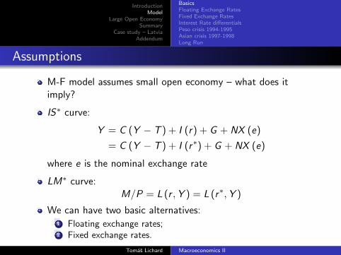
Assumptions

M-F model assumes small open economy – what does itimply?

IS∗ curve:

Y = C (Y − T ) + I (r) + G + NX (e)

= C (Y − T ) + I (r∗) + G + NX (e)

where e is the nominal exchange rate

LM∗ curve:M/P = L (r ,Y ) = L (r∗,Y )

We can have two basic alternatives:1 Floating exchange rates;2 Fixed exchange rates.


IntroductionModel




Subsection 2

Floating Exchange Rates


IntroductionModel




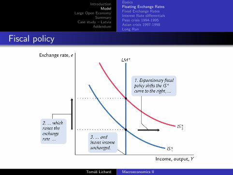
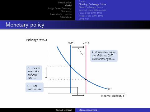
Fiscal policy


IntroductionModel




Monetary policy


IntroductionModel




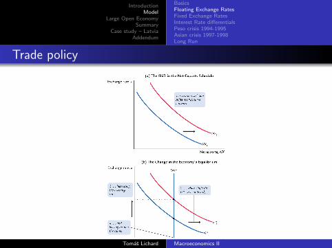
Trade policy


IntroductionModel




Subsection 3

Fixed Exchange Rates


IntroductionModel




How are exchange rates fixed?

CB buy or sell domestic currency for foreign currency to whichthe domestic currency is fixed; however it may run out offoreign reserves (speculative attack – self-fulfilling prophecy)

One solution: currency board – CB holds enough reserves forthe whole domestic currency to be exchanged for the foreignone at the fixed rate

In the real world, usually neither fixed rate nor float is pure(think of CNB and its interventions)


IntroductionModel




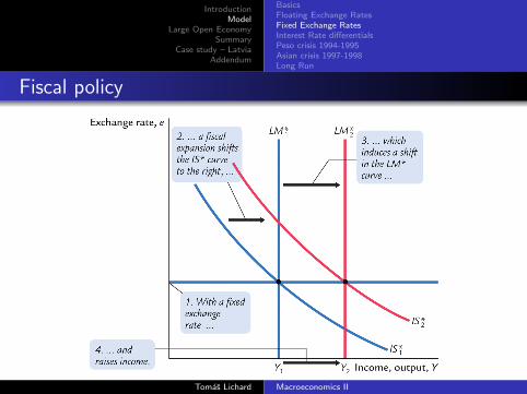
Fiscal policy


IntroductionModel




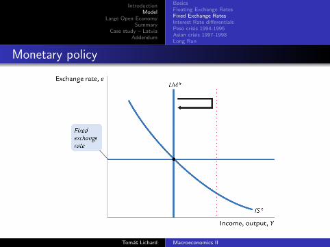
Monetary policy


IntroductionModel




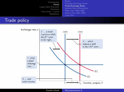
Trade policy


IntroductionModel




Subsection 4

Interest Rate differentials


IntroductionModel




Interest rates differ...

While building M-F model, we assumed r = r∗

But we see in real life that interest rates differ across countries

This can be explained by:

country risk: some countries may be considered unsafe forinvestment due to e.g. political reasons (instability etc)exchange rate expectations Theory of interest rate parity


IntroductionModel




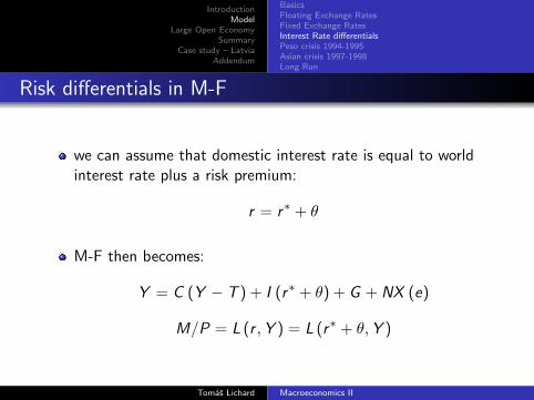
Risk differentials in M-F

we can assume that domestic interest rate is equal to worldinterest rate plus a risk premium:

r = r∗ + θ

M-F then becomes:

Y = C (Y − T ) + I (r∗ + θ) + G + NX (e)

M/P = L (r ,Y ) = L (r∗ + θ,Y )


IntroductionModel




Risk differentials in M-F

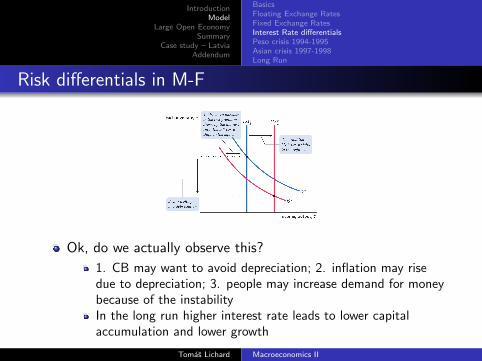
Ok, do we actually observe this?

1. CB may want to avoid depreciation; 2. inflation may risedue to depreciation; 3. people may increase demand for moneybecause of the instabilityIn the long run higher interest rate leads to lower capitalaccumulation and lower growth


IntroductionModel




Subsection 5

Peso crisis 1994-1995


IntroductionModel




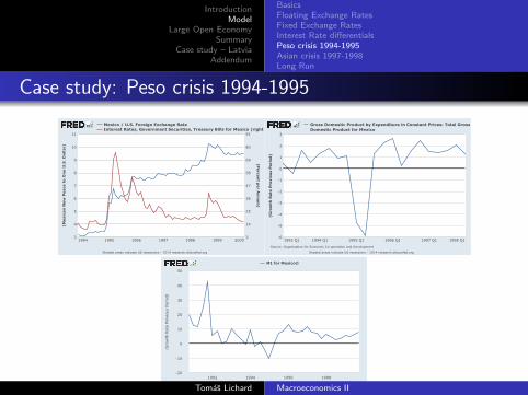
Case study: Peso crisis 1994-1995

NAFTA ratification caused confidence in the Mexicaneconomy, lending increased

However, soon political instability (Zapatista uprising, Colosioassassination) caused increased uncertainty

Fixation of peso to USD lead to decreasing money supply,dollar reserves were spent (Mexico had to abandon the peg),stock markets plummeted

Peso devaluated by approx. 50% w.r.t. dollar

IMF and USA eventually provided guarantees, which calmedthe situation


IntroductionModel




Case study: Peso crisis 1994-1995

(MexicanNewPesostoOneU.S.Dollar)

(Perce

ntp

erA

nnum)

Mexico/U.S.ForeignExchangeRateInterestRates,GovernmentSecurities,TreasuryBillsforMexico(right)

1995 20001994 1996 1997 1998 1999

5

10

3

4

6

7

8

9

11

3

14

25

36

47

58

69

80

91

ShadedareasindicateUSrecessions-2014research.stlouisfed.org

(Gro

wth

Rate

Pre

vio

us

Period)

Source:OrganisationforEconomicCo-operationandDevelopment

GrossDomesticProductbyExpenditureinConstantPrices:TotalGrossDomesticProductforMexico

1995Q11993Q1 1994Q1 1996Q1 1997Q1 1998Q1-6

-5

-4

-3

-2

-1

0

1

2

3


-20

-10

0

10

20

30

40

50

1992 1994 1996 1998

2015research.stlouisfed.org


M1forMexico©

(GrowthRatePreviousPeriod)


IntroductionModel




Subsection 6

Asian crisis 1997-1998


IntroductionModel




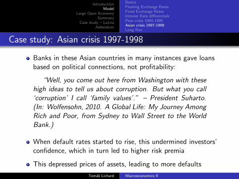
Case study: Asian crisis 1997-1998

Banks in these Asian countries in many instances gave loansbased on political connections, not profitability:

“Well, you come out here from Washington with thesehigh ideas to tell us about corruption. But what you call‘corruption’ I call ‘family values’.” – President Suharto.(In: Wolfensohn, 2010. A Global Life: My Journey AmongRich and Poor, from Sydney to Wall Street to the WorldBank.)

When default rates started to rise, this undermined investors’confidence, which in turn led to higher risk premia

This depressed prices of assets, leading to more defaults


IntroductionModel




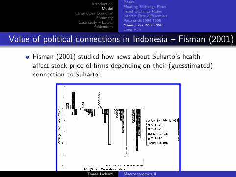
Value of political connections in Indonesia – Fisman (2001)

Fisman (2001) studied how news about Suharto’s healthaffect stock price of firms depending on their (guesstimated)connection to Suharto:

ascertain the date when rumors first hit theJakarta Exchange—there was generally a spe-cific triggering event, which I take as the start ofthe episode. I assumed that each episode cameto an end when it was (1) explicitly put to restby the revelation of new information or (2) itwas reported that analysts had factored the newinformation about Suharto’s health into theirpricing of securities.

II. Results

Figure 1 shows the share price returns for thesix episodes, with the Suharto Dependency In-dex on the horizontal axis. The graph stronglysuggests that politically dependent firms, on av-

erage, lost more value during these episodesthan did less-dependent firms.To get a sense of the magnitude of the effect

of political dependence during each episode, Iran a set of regressions using the followingspecification:

(1) Rie ! " # $ ! POLi # % ie

where Rie is the return on the price of securityi during episode e, POLi is the firm’s SuhartoDependency Number, and %ie is the error term.5The results of this set of regressions are listed inTable 2; consistent with the raw pattern illus-trated in Figure 1, $ is negative in everyinstance.Now, in each episode, investors were reacting

to a different piece of news, so we expect thecoefficient on POLi to differ across events.More precisely, a more severe threat to Suhar-to’s health should intensify the effect of politi-cal dependence, hence the magnitude of $should be increasing with event severity. As ameasure of the market’s concerns regarding thethreat to Suharto’s health in each episode, I use

5 All regressions reported in this paper use standarderrors that correct for heteroskedasticity. I also ran regres-sions using an error structure that only allowed for thecorrelation of %eis for each company, i.e., Cov(%ei , %fj) ! 0 ifand only if i " j. The regressions were also run using anerror structure that allowed for the correlation of %eis withineach group. These various approaches yielded very similarsets of standard errors.

TABLE 1—SUMMARY STATISTICS BY DEGREE OF POLITICAL DEPENDENCE AS MEASUREDBY THE SUHARTO DEPENDENCY INDEX

POL 1 2 3 4 5 All firms Observations

Observations 5 34 10 16 14 79

Assets2,145.76(2,843.63)

2,228.57(3,989.85)

2,206.20(3,676.99)

1,634.08(2,561.07)

1,765.51(2,230.52)

2,033.19(3,321.59) 76

Debt707.18(702.84)

791.32(1,478.83)

813.25(976.28)

397.83(461.06)

712.57(1,070.83)

717.37(1,186.85) 70

Return on assets(net income)/(total assets)

0.038(0.031)

0.058(0.058)

0.043(0.023)

0.037(0.032)

0.050(0.029)

0.050(0.044) 76

Tax rate (taxespaid)/(pretaxincome)

0.23(0.05)

0.24(0.12)

0.16(0.14)

0.22(0.16)

0.15(0.12)

0.21(0.13) 74

Sources: All data are from the Financial Times’ Extel Database (1997); Assets and Debt are expressed in millions of 1995rupiah.

FIGURE 1. EFFECT OF POLITICAL DEPENDENCE ON SHAREPRICE RETURNS

1098 THE AMERICAN ECONOMIC REVIEW SEPTEMBER 2001


IntroductionModel




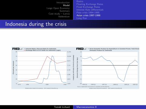
Indonesia during the crisis

(PercentperAnnum)

(Natio

nalCurre

ncyUnitsp

erU

SDollar)

InterestRates,DiscountRateforIndonesiaExchangeRatetoU.S.DollarforIndonesia(right)

20001970 1996 199810

20

30

40

50

60

70

80

1,400

2,843

4,286

5,729

7,172

8,615

10,058

11,501


(Perc

en

tC

han

gef

rom

Year

Ag

o)


GrossDomesticProductbyExpenditureinConstantPrices:TotalGrossDomesticProductforIndonesia

1995Q1 2000Q11996Q1 1997Q1 1998Q1 1999Q1-20

-15

-10

-5

0

5

10

15



IntroductionModel




Subsection 7

Long Run


IntroductionModel




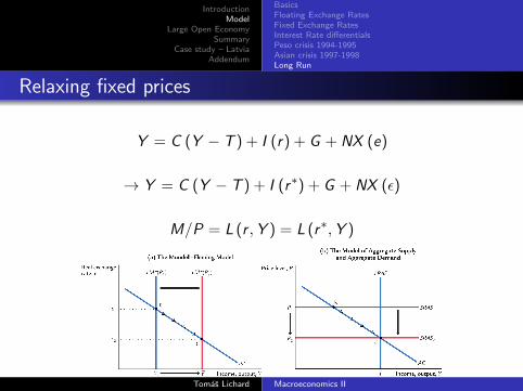
Relaxing fixed prices

Y = C (Y − T ) + I (r) + G + NX (e)

→ Y = C (Y − T ) + I (r∗) + G + NX (ε)

M/P = L (r ,Y ) = L (r∗,Y )


IntroductionModel



Section 3

Large Open Economy


IntroductionModel



Basics

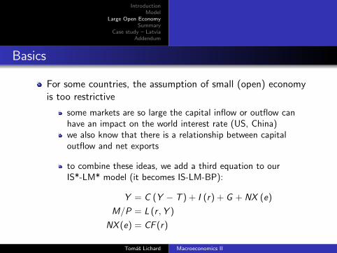
For some countries, the assumption of small (open) economyis too restrictive

some markets are so large the capital inflow or outflow canhave an impact on the world interest rate (US, China)we also know that there is a relationship between capitaloutflow and net exports

to combine these ideas, we add a third equation to ourIS*-LM* model (it becomes IS-LM-BP):

Y = C (Y − T ) + I (r) + G + NX (e)

M/P = L (r ,Y )

NX (e) = CF (r)


IntroductionModel



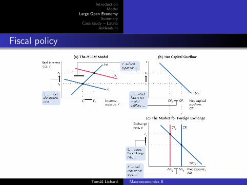
Fiscal policy


IntroductionModel



Section 4

Summary


IntroductionModel



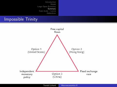
Impossible Trinity


IntroductionModel



Section 5

Case study – Latvia


IntroductionModel




Advocates of “internal devaluation” were often pointing out toLatvia as a success storyMacroeconomic policies that were used to respond to the2009 recession:

maintaining fixed exchange rate w.r.t. Eurodesire to decrease debt (or at least avoid its increase) led topro-cyclical fiscal policyfor the most part, also pro-cyclical monetary policy wasadopted (partly because of the peg)

The goal was the “internal devaluation” to increasecompetitivness:

decrease in unit labor costs due to pressure of unemploymentdecrease public payroll (lower wages of publicemployees/layoffs)however, these decreased aggregate demand even further


IntroductionModel




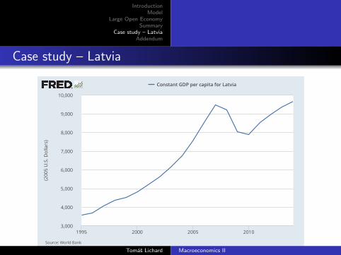
3,000

4,000

5,000

6,000

7,000

8,000

9,000

10,000

1995 2000 2005 2010

research.stlouisfed.orgSource:WorldBank

ConstantGDPpercapitaforLatvia

(2005U.S.D

ollars)


IntroductionModel



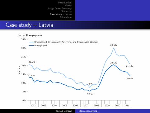
Case study – LatviaCEPR Latvia's Internal Devaluation: A Success Story? z 9

FIGURE 4 Latvia: Unemployment

Note: Unemployment is measured as a percent of the active labor force. Unemployed, involuntarily part-time, and discouraged workers are measured as a percent of the active labor force plus discouraged workers. Source: Latvijas Statistika (2011) and authors’ calculations. It also does not include all the people who have left the country in search of employment since the crisis began. It is estimated that the net loss of population in 2009-2011 amounts to as many as 120,000 people, or 10 percent of the labor force.6 If not for this migration, the broader measure of unemployment could be as high as 29 percent in the third quarter of 2011, instead of 21.1 percent. Another way to evaluate the impact of the crisis and economic policy on the labor market is to look at employment. This is shown in Figure 6. Employment dropped about 20.3 percent from its peak in the fourth quarter of 2007 to the bottom in the first quarter of 2010. Since the economy began recovering, it has recovered just 6.0 percentage points of this loss, leaving Latvia with 14.3 percent fewer working-age people employed as compared to pre-crisis employment. 6 Official data shows a much lower flow, but this data does not capture most of the people who emigrate. Studies using

data on Latvian migrants in the countries where they emigrate to have yielded the much higher and more realistic figures cited above. In fact, Hazans cites data showing that emigration, which he puts at 80,000 between 2009 and 2010, actually accelerated in 2011; thus, 120,000 over three years can be seen as a conservative estimate. For more on Latvian emigration, see Hazans (2011a), 2011b, Hazans and Philips (2011), and Holland et al. (2011).

20.5%

7.5%

30.1%

21.1%

12.9%

5.3%

20.5%

14.4%

0%

5%

10%

15%

20%

25%

30%

35%

2002 2003 2004 2005 2006 2007 2008 2009 2010 2011

Perc

ent

Unemployed, Involuntarily Part-Time, and Discouraged Workers

Unemployed

Source: Weisbrot&Rey (2011)Tomas Lichard Macroeconomics II

IntroductionModel



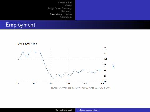
Employment


IntroductionModel



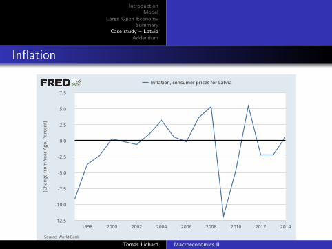
Inflation

-12.5

-10.0

-7.5

-5.0

-2.5

0.0

2.5

5.0

7.5

1998 2000 2002 2004 2006 2008 2010 2012 2014

research.stlouisfed.orgSource:WorldBank

Inflation,consumerpricesforLatvia

(Cha

ngefrom

Yea

rAg

o,Perce

nt)


IntroductionModel



Case study – LatviaCEPR Latvia's Internal Devaluation: A Success Story? z 13

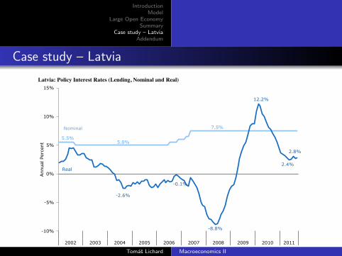
FIGURE 9 Latvia: Policy Interest Rates (Lending, Nominal and Real)

Source: European Commission (2011), Latvijas Statistika (2011), and authors’ calculations. The result of these changes is that Latvia’s recovery was spurred by macroeconomic policies that went against the strategy of “internal devaluation.” In other words, the government of Latvia adopted an “internal devaluation” strategy that included massive fiscal tightening, rising real interest rates, depression-level unemployment rates, and deflation. The economy suffered the worst collapse in the world for 2008-2009. Then policy was reversed: fiscal policy was neutral for 2010; monetary policy became expansionary, because external shocks raised the inflation rate. The inflation also lowered the country’s debt burden, as noted above. This increased investor and consumer confidence (including confidence that the peg would hold, which facilitated the maintenance of more expansionary monetary policy). It is important to remember that the inflation also went against the government’s policy of internal devaluation, which relies on lowering inflation, or even deflation as occurred in 2009, to lower the real exchange rate. But this burst of inflation was very important to the recovery.

Because these macroeconomic policies and the inflationary shock were much more expansionary than the program that the government was committed to, the economy was able to get out of the downward spiral that had caused the IMF to project such a pessimistic forecast at the end of 2009.

It is true that there was some internal devaluation; according to the IMF, the real effective exchange rate, based on unit labor costs, depreciated by about 21 percent from its peak at the beginning of 2009, to the third quarter of 2010. On a CPI (consumer price index) basis, the depreciation was about nine percent from a peak in March 2009 to March 2011. Although exports increased from

5.5% 5.0%

7.5%

-2.6%

-0.1%

-8.8%

12.2%

2.4%

2.8%

-10%

-5%

0%

5%

10%

15%

2002 2003 2004 2005 2006 2007 2008 2009 2010 2011

Ann

ual P

erce

nt

Real

Nominal

Source: Weisbrot&Rey (2011)


IntroductionModel



Trade

CEPR Latvia's Internal Devaluation: A Success Story? z 14

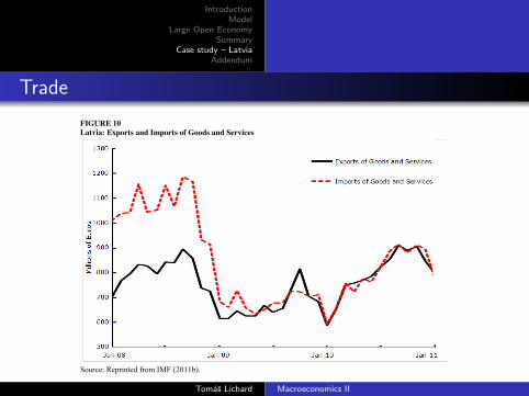
January 2010 onward, imports increased commensurately; so there has so far been little or no contribution to the recovery from net exports following the internal devaluation. This can be seen in Figure 10. This must be emphasized because the end goal of the internal devaluation strategy is to boost the economy through an increase in net exports. As can be seen in Figure 10, there is almost no increase in net exports since the economy began to expand at the beginning of 2010. Furthermore – and again this must be emphasized, the plunge in imports – which eliminated the trade deficit – took place before there was any real depreciation of the exchange rate. The real exchange rate did not begin to depreciate until the first quarter of 2009 (by the Unit Labor Cost Measure), or even later (2nd quarter 2009) by the CPI measure. As can be seen from Figure 10, the collapse of imports occurs before the first quarter of 2009, mainly due to the collapse of aggregate demand as a result of the deep recession. FIGURE 10 Latvia: Exports and Imports of Goods and Services

Source: Reprinted from IMF (2011b).

Source: Weisbrot&Rey (2011)Tomas Lichard Macroeconomics II

IntroductionModel



Section 6

Addendum


IntroductionModel



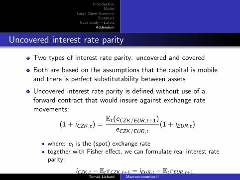
Uncovered interest rate parity

Two types of interest rate parity: uncovered and covered

Both are based on the assumptions that the capital is mobileand there is perfect substitutability between assets

Uncovered interest rate parity is defined without use of aforward contract that would insure against exchange ratemovements:

(1 + iCZK ,t) =Et(eCZK/EUR,t+1)

eCZK/EUR,t(1 + iEUR,t)

where: et is the (spot) exchange ratetogether with Fisher effect, we can formulate real interest rateparity:

iCZK ,t − EtπCZK ,t+1 = iEUR,t − EtπEUR,t+1Tomas Lichard Macroeconomics II

IntroductionModel



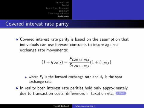
Covered interest rate parity

Covered interest rate parity is based on the assumption thatindividuals can use forward contracts to insure againstexchange rate movements:

(1 + iCZK ,t) =FCZK/EUR,t

SCZK/EUR,t(1 + iEUR,t)

where Ft is the forward exchange rate and St is the spotexchange rate

In reality both interest rate parities hold only approximately,due to transaction costs, differences in taxation etc. Back


Documents

Macroeconomics II - CERGE-EI