Attention Please!∗

Olivier Gossner

CREST, CNRS, Ecole Polytechnique

and London School of Economics

Jakub Steiner

University of Zurich and CERGE-EI

Colin Stewart

University of Toronto

December 3, 2020

Abstract

We study the impact of manipulating the attention of a decision-maker who learns

sequentially about a number of items before making a choice. Under natural assump-

tions on the decision-maker’s strategy, directing attention toward one item increases its

likelihood of being chosen regardless of its value. This result applies when the decision-

maker can reject all items in favor of an outside option with known value; if no outside

option is available, the direction of the effect of manipulation depends on the value of

the item. A similar result applies to manipulation of choices in bandit problems.

keywords: sequential sampling, marketing, persuasion, attention

JEL codes: D8, D91

1 Introduction

The struggle for attention is a pervasive phenomenon. Attention-seeking behavior plays

an important role in advertising, finance, industrial organization, psychology, and biology.1

∗We have benefited from discussions with Ian Krajbich, Arina Nikandrova, Marco Ottaviani, Ryan Webb,Andy Zapechelnyuk, and participants at various seminars and conferences. Pavel Ilinov, Jan Sedek, and JiaqiZou provided excellent research assistance. This work was financially supported by the French NationalResearch Agency (ANR), “Investissements d’Avenir” (ANR-11-IDEX0003/LabEx Ecodec/ANR-11-LABX-0047) (Gossner), ERC grant 770652 (Steiner), and by the Social Sciences and Humanities Research Councilof Canada (Stewart).

1See, e.g., Fogg-Meade (1901) for advertising, Lou (2014) for finance, Eliaz and Spiegler (2011) forindustrial organization, Orquin and Loose (2013) for psychology, and Dukas (2002) for biology.

1

The main message is consistent across fields: drawing attention toward an item increases its

demand.

The existing literature provides two main explanations for how grabbing attention can

increase demand.2 One is that it directly affects preferences. While difficult to disprove,

a theory of changing preferences offers limited predictive power and makes welfare analysis

challenging. The other major explanation is that attention-grabbing behavior itself conveys

information—either directly or through signaling—and thereby changes beliefs. But this

second channel alone does not suffice to explain the empirical evidence. In fact, there is

a sizable body of evidence showing that manipulating attention has a direct influence on

demand even when devoid of information.3

We identify a mechanism through which grabbing attention increases demand without

influencing preferences or changing the information available to the decision-maker. We

consider a decision-maker who learns sequentially about the quality of a number of items

by allocating her attention to one of the items in each period. Paying attention to an item

generates noisy information about its value. Due to cognitive (or other) limitations, the

decision-maker can focus on only one item at a time; while she pays attention to a given

item, her assessment of its value evolves stochastically, while her assessments of the other

items remain the same. In our main model, once her assessment of an item is sufficiently

high (according to an exogenously fixed threshold), she stops and chooses that item, and if

her assessments of all items are sufficiently low, she stops and chooses an outside option.

In the context of consumer marketing, we think of the items as substitutable brands of

a good, and the outside option as the choice not to purchase any item. Starting from a

given strategy governing the decision-maker’s attention, we introduce an attention-grabbing

manipulation that induces the decision-maker to focus more on one “target” item (perhaps

only for a limited time). We show that, under general conditions, such a manipulation

increases demand for the target item.

The decision-maker’s learning is governed by an attention strategy that maps assessments

in any given time period to a (possibly random) item of focus. An attention strategy gener-

ates, for each profile of values of the items, a stochastic process over assessments and items

of attention, and a probability that each item is chosen. We refer to these probabilities

as interim demands for the items. The impact of attention manipulation is captured by

the difference in interim demands under the baseline and manipulated attention strategies;

the baseline strategy is the one the decision-maker employs in the absence of manipulation,

while the manipulated strategy induces the decision-maker to increase her focus on a target

2See Bagwell (2007) for a survey in the context of advertising.3See, e.g., Chandon et al. (2009), Krajbich and Rangel (2011), or, for a survey, Orquin and Loose (2013).

2

item at each profile of assessments and in each period, but agrees with the baseline strategy

conditional on not focusing on the target item.

We show that manipulation of attention increases demand and decreases the time to

decision in favor of the target item (in the sense of first-order stochastic dominance). This

increase in demand comes at the expense of each of the other items, for which demand

decreases and the time to decision increases. These results hold for any realization of the

items’ values. In particular, manipulating attention increases demand even if the target item

is worse than the other items and the outside option.

The key to understanding the effect of manipulation is to consider the path of learning for

each possible realization of the sequence of signals for each item. Given such a realization, we

can view an attention strategy as selecting, in each period, an item for which to uncover one

more step along the sequence. The choice of item at the end of the process can be thought of

as resulting from a kind of approval contest: the decision-maker continues to learn until she

approves of one of the items, or until she finds all of them to be unworthy of approval. For a

given realization of the sequences of signals, there may be multiple items the decision-maker

would approve of were she to pay enough attention to them. The choice then comes down

to which of these items she approves of first. Directing attention toward one of these items

accelerates the process of approval for this item while slowing it down for the other items.

Consequently, the likelihood that the target item is chosen increases.

This simple intuition ignores the significant complication that manipulating attention

generally affects future attention choice. It could happen that, for some attention strategies,

temporary manipulation toward a target item leads to a path along which the decision-maker

pays much less attention to the target item afterwards, more than compensating for the direct

effect of increased attention. If there are only two items (not including the outside option),

then this cannot happen: our results hold regardless of the baseline attention strategy.

With more than two items, we require two additional assumptions on the attention strategy.

First, the attention strategy should be stationary: focus in each period must depend only

on the current assessment, not on the current time. The second assumption is a form of

independence of irrelevant alternatives (IIA): conditional on not focusing on the target item

i, the probability of focusing on each other item is independent of the belief about the value

of item i (though it may depend on the beliefs about items other than i). Together, these

two assumptions allow us to consider learning about the target item separately from learning

among the remaining items, effectively reducing the problem to one with two items.

A similar but simpler result applies to manipulation of choices in multi-armed bandit

problems. In this framework, the decision-maker chooses an arm in each period and revises

her assessment of an arm after each time she chooses it. We show that, under general

3

conditions, manipulating choice toward a target arm never reduces the number of times it is

chosen up to any period. Even if the manipulation ends after a limited time, the decision-

maker’s subsequent choices never overcome the initial increase in the choice of the target

arm. In particular, introducing one arm before the others cannot lead to a reduction in the

total number of times that arm is chosen up to any given period.

To formalize these intuitions, we rely on a technique known in probability theory as

coupling (as in, e.g., Lindvall, 1992). In short, we construct a joint probability space in

which we fix, for each item, the outcome of the learning process that would arise if the

decision-maker focused only on that item. We refer to a profile of realizations of these

learning processes across items as a draw ; that is, a draw is a state in the joint probability

space. Given any draw, the decision-maker’s strategy determines the realization of the

learning process. The strategy affects only the timing of the process for each item, not

the signal realizations or their ordering. We show that, with this coupling, for every draw,

manipulating attention toward an item both increases demand for that item and decreases

decision time if that item is chosen.

Both stationarity and IIA are needed for our results in the sense that their conclusions do

not hold if we dispense with either assumption; we provide counterexamples in Section 5.1

and Appendix B. Both assumptions, though restrictive, are automatically satisfied if the

attention strategy is optimized given the stopping rules in our main model: we prove that,

for a general class of learning costs, optimal attention strategies have a (stationary) Gittins

index structure as in the theory of multi-armed bandits. It follows that these strategies are

stationary and satisfy IIA.

The presence of an outside option motivates the stopping rule employed by the decision-

maker in our main model as a form of satisficing behavior. Such an outside option appears

naturally in consumer choice as the option not to purchase any item, and in finance as the

option to invest in a risk-free asset. Our stopping rule implicitly assumes that the value

of the outside option is not so low that the decision-maker would reject it in favor of an

item she has not inspected, nor so high that she would choose it in favor of such an item.

If there were no outside option (or the value of the outside option was low), the decision-

maker could choose by a process of elimination rather than approval; that is, she could seek

to eliminate items that she believes to be bad and ultimately choose an item—the last one

remaining—with little knowledge of its value. In this case, manipulating attention toward an

item may increase the chance that it is eliminated before the other items, thereby decreasing

the demand for it. Moreover, in the limit as learning becomes arbitrarily precise, we find

that, for any stationary attention strategy that satisfies IIA, manipulation increases demand

4

for the target item if its value is high, and decreases demand if its value is low.4

Our results can operate on a variety of timescales. Over a short time horizon, we envision

a consumer choosing among several brands at the point of purchase. In this case, learning

may consist primarily of introspection about the current desirability of each item, includ-

ing recall of past experience consuming the item. Attention can be manipulated through

placement of products on the shelf or webpage, or through previous exposure to advertising

that increases the likelihood of a particular brand coming to mind (e.g., through the recency

effect). Over a longer time horizon, a decision-maker could be repeatedly choosing among

brands of some item and learning about her taste for each brand through her experience con-

suming it. In this case, manipulation in our model corresponds to any change that boosts

consumption (temporarily or permanently) of a particular brand, such as introductory sale

pricing. Our results also apply to changes in the time at which items are introduced: one

item entering the market before the others is equivalent to manipulation in favor of that

item at the beginning of the process. Clinical trials, which we discuss in Section 6.1, are

another application of our model with a relatively long time horizon.

Our result is robust to many aspects of the learning process. The information structure

for each item is general, allowing for any number of signal realizations and dependence on

the current assessment of the item. The decision-maker need not be Bayesian; we can, for

instance, interpret her assessments as intensities of accumulated neural stimuli in favor of

each item (as, e.g., in Platt and Glimcher, 1999), which can evolve according to an arbitrary

stationary Markov process. We also allow for general attention strategies, whether optimal

with respect to some cost structure or not.

When applied to advertising, our model has distinctive predictions compared to theories

of informative advertising (Stigler, 1961; Telser, 1964), signaling (Nelson, 1974), comple-

mentary advertising (Stigler and Becker, 1977; Becker and Murphy, 1993), and persuasive

advertising (Braithwaite, 1928; Kaldor, 1950). Unlike these theories, manipulation in our

model is not associated with a systematic change in the consumer’s assessments of the values

of the items. Data combining consumers’ choices and beliefs can therefore be used to test

among these theories. For example, Atalay et al. (2012) find experimentally that placement

of a product in the horizontal center of a display is associated with increased likelihood of

choice but not with inferences about the quality of the corresponding brand. They argue that

the effect of horizontal placement is due to greater attention being paid to central items, as in

our model. Our theory also provides novel predictions regarding timing. First, manipulation

reduces the time to choose the target item and increases the time for other items. Second,

4This is reminiscent of the experimental finding in Armel et al. (2008) that manipulating attention tendsto increase the choice probability for “appetitive” items and decrease the probability for “aversive” ones.

5

as noted above, earlier introduction of an item is associated with an increase in demand.

Related literature Evidence that increased attention boosts demand comes from several

fields. In marketing, Chandon et al. (2009) show that drawing attention to products—

for instance, with large displays or placement at eye level—increases demand. In finance,

Seasholes and Wu (2007) show that attention-grabbing events about individual stocks in-

crease demand for them. In biology, Yorzinski et al. (2013) study the display strategies

through which peacocks grab and retain the attention of peahens during courtship. In each

of these contexts, the decision-maker has an outside option not to choose any available item;

our results suggest that this is an important feature driving the effect of attention-grabbing

behavior on demand.

Our assumptions on attention allocation are rooted in psychology. Though humans are

able to pay attention to multiple stimuli simultaneously, such division of attention is difficult,

especially when the stimuli are similar to each other (e.g., Spelke, Hirst, and Neisser, 1976).

Psychologists distinguish between exogenous and endogenous attention, where the first is

beyond the decision-maker’s control and is triggered by sudden movements, bright colors

and such, while endogenous attention shifts are controlled by the decision-maker (Mayer

et al., 2004). Manipulation of attention in our model could be exogenous in this sense, while

the baseline attention strategy could be endogenous.

Our model builds on a long tradition in statistics and economic theory originating with

Wald (1945), who proposed a theory of optimal sequential learning about a single binary

state. A growing literature studies optimal sequential learning about several options when

attention must focus on one item at a time (Mandelbaum, Shepp, and Vanderbei, 1990;

Ke, Shen, and Villas-Boas, 2016; Ke and Villas-Boas, 2019; Nikandrova and Pancs, 2018;

Austen-Smith and Martinelli, 2018). The structure of the optimal learning strategy varies

depending on the costs and information structure. Our results on the impact of attention

manipulation are independent of these considerations; however, relative to this literature,

we make simplifying assumptions on the rules that govern termination of learning. In a

different vein, Che and Mierendorff (2019) study sequential allocation of attention between

two Poisson signals about a binary state. In contrast, in our model, the decision-maker

chooses among signals about multiple independent states.

In the drift-diffusion model of Ratcliff (1978), a decision-maker tracks the difference in the

strength of supporting evidence between two actions, making a choice when this difference

becomes sufficiently large.5 Krajbich, Armel, and Rangel (2010) explicitly incorporate atten-

tion choice in this model and introduce an exogenous bias in the accumulated signal toward

5Ratcliff’s model is essentially equivalent to a sequential sampling model along the lines of Wald (1945).

6

the item on which the decision-maker is currently focusing. This extended drift-diffusion

model accommodates empirical findings showing that exogenous shifts in attention tend to

bias choice (see, e.g., Armel, Beaumel, and Rangel, 2008; Milosavljevic et al., 2012). The

closest drift-diffusion models to ours are the so-called “race models” in which evidence in

support of distinct alternatives is integrated in separate accumulators, with the choice driven

by whichever accumulator reaches its stopping boundary first; see Bogacz et al. (2006) for

a review. Relative to this literature, whose primary modeling goal is to fit choice data, we

focus on foundations for the mechanism by which attention affects demand.

Optimal sequential learning about several items is related to the theory of multi-armed

bandits (Gittins and Jones, 1974). In addition to applying our main result to bandit prob-

lems, we exploit this connection to show that optimal attention strategies in our model of

one-shot choice satisfy IIA by using the Gittins index characterization.

2 Simplified setting

Before presenting the model in its full generality, we introduce the main ideas in two par-

ticularly simple environments in which temporarily manipulating attention toward an item

increases its demand. These two environments differ in how choices of items relate to learn-

ing, but the mechanism behind the effect of manipulation is the same.

In both environments, a decision-maker (DM) learns sequentially about two items j ∈{1, 2} with unknown values vj ∈ {−1, 1}. In each period t = 0, 1, . . ., the DM focuses on

an item ιt ∈ {1, 2}. Focusing on an item generates a signal xt about the value of that item

which is independent of the value of the other item. Conditional on the values, signals are

independent across periods. In this section, the signal takes a simple form: for each item,

the possible signal realizations are −1 and 1, and for each value v, the realized signal about

an item of value v is equal to v with probability λ > 1/2; that is, Pr(xt = 1 | vιt = 1) = λ =

Pr(xt = −1 | vιt = −1).

For each j and t, let

pjt =∑

s<t:ιs=j

logPr (xs | vj = 1)

Pr (xs | vi = −1)= log

(λ

1− λ

) ∑s<t:ιs=j

xs. (1)

Thus pjt is the log-likelihood ratio (LLR) comparing vj = 1 to vj = −1 given the observed

signals about item j up to the beginning of period t. We write pt for the pair (p1t , p

2t ).

Attention allocation is governed by a (pure) attention strategy α : R2 −→ {1, 2} that specifies

7

the item of focus ιt = α(pt) for each pair pt of LLRs.6

2.1 Manipulation of attention

In order to understand how manipulation of attention affects choice, we first examine how

it affects subsequent attention allocation.7 To this end, given a baseline strategy β, we

introduce a manipulated strategy µ constructed from β by making item 1 the item of focus

in the initial period and then returning to β in all subsequent periods. That is, the item of

focus µ(p, t) in period t for LLRs p is given by

µ(p, t) =

1 if t = 0,

β(p) if t > 0.

For each t, let kt denote the cumulative focus on item 1 before period t under the baseline

strategy β; that is,

kt = |{s < t : β(ps) = 1}|.

Similarly, let kt denote the analogous cumulative focus under the manipulated strategy µ.

While manipulation clearly increases attention to item 1 in the first period, subsequent

allocation of attention could, in principle, more than compensate for this effect and cause

item 1 to eventually receive less attention than it would without manipulation. The fol-

lowing result indicates that this cannot happen: manipulation never decreases the attention

allocated to item 1.

Proposition 1. For each t ≥ 1 and all pairs of values v, kt (weakly) first-order stochastically

dominates kt.8

This proposition is a special case of Proposition 3; accordingly, we omit its proof.

To compare the allocation of attention under the two strategies, we “couple” the resulting

processes governing the LLRs; that is, we define them on a common probability space in

a way that enables us to make comparisons realization-by-realization. In this section, we

describe this construction informally; a precise treatment is provided in Section 3.1.

6One could equivalently formulate the model in terms of a Bayesian decision-maker whose attentionstrategy is a function of posterior beliefs about the values.

7We do not explicitly model how attention is manipulated. Depending on the context, manipulationcould result from changes in visual salience, in relative inspection costs, or in the position of the items on alist (as in online search results).

8Recall that a random variable σ (weakly) first-order stochastically dominates another random variableσ′ if Pr(σ ≤ t) ≤ Pr(σ′ ≤ t) for every t. We henceforth drop the “weakly” qualifier.

8

For this construction, fix v, and imagine that there is a large (countably infinite) deck of

cards for each item, with each card showing a signal realization of −1 or 1 (with probabilities

as described above). Beginning with all cards in each deck face down, in each period t, the

baseline attention strategy selects a deck from which to draw the next card according to the

item of focus ιt = β(pt). The DM updates the relevant LLR based on the signal shown on the

card that was drawn. Now consider the effect of manipulation for a given sequence of cards

in each deck, where manipulation induces the first card to come from the deck for item 1.

To avoid trivialities, suppose that, absent manipulation, the DM first draws from deck 2.

Manipulation can have persistent and complicated effects on attention allocation by taking

the DM to different path of LLRs pt. And yet, as Proposition 1 indicates, the subsequent

allocation of attention can never overtake the direct effect of manipulation: the cumulative

attention devoted to the target item can only increase as a result of manipulation.

The key observation is that, once the ordering of the cards is fixed, we only need to

keep track of how many cards the baseline and manipulated strategies draw from each deck,

and can disregard the order in which the decks are chosen. At the end of the first period,

compared to the baseline strategy, the manipulated strategy is further ahead with deck 1

(in the sense that more cards have been drawn from deck 1). Correspondingly, the baseline

strategy is further ahead with deck 2. In each subsequent period, either the manipulated

strategy remains ahead with deck 1 (perhaps pulling even further ahead) and the baseline

strategy remains ahead with deck 2, or the numbers of draws from both decks under the

baseline strategy “meet” the numbers under the manipulated strategy. In the latter case,

LLRs and attention allocation coincide under the two processes following the period in which

they meet. Either way, regardless of the ordering of the cards, for any baseline attention

strategy, and up to any period t, cumulative focus on item 1 is at least as large under the

manipulated strategy as under the baseline strategy, and correspondingly, the cumulative

focus on item 2 is at least as large under the baseline strategy as under the manipulated one.

Our interest in how manipulation affects attention allocation is driven by its consequent

effect on choice. The following two subsections present settings in which increased attention

leads to an unambiguous increase in demand.

2.2 One-shot choice

First, we consider a DM who decides when to stop learning and make a one-shot choice

among the two items j ∈ {1, 2} and an outside option with a known value. We focus on

a simple stopping rule that adapts Simon’s (1955) model of satisficing to allow for gradual

learning and the presence of an outside option. If, at any point in the process, the DM has

9

collected enough evidence that one of the items is of high value, she stops and chooses that

item. If, on the other hand, she has collected enough evidence that both items are of low

value, she stops and chooses neither item (i.e., chooses the outside option). Accordingly,

we introduce thresholds p < 0 < p and define stopping regions F j = {p : pj ≥ p} for

j = 1, 2, F oo = {p : pj ≤ p for j = 1, 2} and F = F 1 ∪ F 2 ∪ F oo. Learning stops in period

τ = min{t : pt ∈ F} with the DM choosing item j if pτ ∈ F j and the outside option

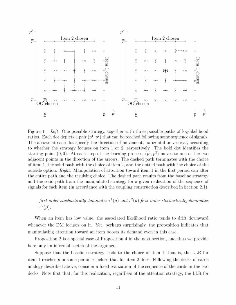
if pτ ∈ F oo. (Stopping in F 1, F 2, and F oo are mutually exclusive.) See Figure 1 for an

illustration.9

Let τ j denote the period in which the DM chooses item j; that is, τ j = τ if item j

is chosen and τ j = ∞ otherwise. Note that τ and τ j depend on the attention strategy;

accordingly, we write τ(α) and τ j(α) if the attention strategy α is not otherwise clear from

the context.

The above rules specify, for any given pair of values v, the joint stochastic process of

LLRs and focus of attention (pt, ιt)t; we denote by P vα their joint law. For any strategy α

and pair of values v, we let the interim demand for item j,

Dj(v;α) = P vα

(pτ ∈ F j

),

be the probability that the DM stops with the choice of j when the true values are v.

We say that an attention strategy α is non-wasteful if α(p) 6= j whenever p is such that

pj ≤ p and pj′ ≥ p for j′ 6= j. Non-wasteful strategies do not focus on an item that the DM

deems to have low value.

Proposition 2. Suppose that the baseline attention strategy β is non-wasteful. For all pairs

of values v ∈ {0, 1}2, manipulating attention toward item 1 in the first period

1. (weakly) increases the demand for item 1 and decreases the demand for item 2; that is,

D1(v;µ) ≥ D1(v; β)

and D2(v;µ) ≤ D2(v; β),

and

2. accelerates the choice of item 1 and decelerates the choice of item 2; that is, τ 1(β)

9This process is an extension of the sequential probability ratio test of Wald (1945) from two to multiplehypotheses. It also extends the drift-diffusion model of Ratcliff (1978) to allow for choice among threeoptions (including the outside option). In a non-Bayesian, prior-free setting, results on optimal stopping formultiple-hypothesis sequential sampling are scarce, presumably due to the lack of an obvious objective andthe complexity of the problem. An exception is the asymptotic literature originating in Chernoff (1959),who shows that a simple threshold stopping rule is approximately optimal as the cost of sampling vanishes.

10

p1|p

|p

p2

−p

−p

•

•

•

•

•

•

•

•

•

•

•

•

•

•

•

•

•

•

•

•

•

•

•

•

•

•

•

•

•

•

•

•

•

•

•

•

•

•

•

•

•

•

•

•

•

•

•

•

•

•

Item1

chosen

Item 2 chosen

OO chosen

p1|p

|p

p2

−p

−pItem

1ch

osenItem 2 chosen

•

•

•

•

•

•

•

•

•

•

•

•

•

•

•

•

•

•

•

•

•

•

•

•

•

•

•

•

•

•

•

•

•

•

•

•

•

•

•

•

•

•

•

•

•

•

•

•

•

OO chosen

•

Figure 1: Left : One possible strategy, together with three possible paths of log-likelihoodratios. Each dot depicts a pair (p1, p2) that can be reached following some sequence of signals.The arrows at each dot specify the direction of movement, horizontal or vertical, accordingto whether the strategy focuses on item 1 or 2, respectively. The bold dot identifies thestarting point (0, 0). At each step of the learning process, (p1, p2) moves to one of the twoadjacent points in the direction of the arrows. The dashed path terminates with the choiceof item 1, the solid path with the choice of item 2, and the dotted path with the choice of theoutside option. Right : Manipulation of attention toward item 1 in the first period can alterthe entire path and the resulting choice. The dashed path results from the baseline strategyand the solid path from the manipulated strategy for a given realization of the sequence ofsignals for each item (in accordance with the coupling construction described in Section 2.1).

first-order stochastically dominates τ 1(µ) and τ 2(µ) first-order stochastically dominates

τ 2(β).

When an item has low value, the associated likelihood ratio tends to drift downward

whenever the DM focuses on it. Yet, perhaps surprisingly, the proposition indicates that

manipulating attention toward an item boosts its demand even in this case.

Proposition 2 is a special case of Proposition 4 in the next section, and thus we provide

here only an informal sketch of the argument.

Suppose that the baseline strategy leads to the choice of item 1; that is, the LLR for

item 1 reaches p in some period τ before that for item 2 does. Following the decks of cards

analogy described above, consider a fixed realization of the sequence of the cards in the two

decks. Note first that, for this realization, regardless of the attention strategy, the LLR for

11

item 1 can never reach p before it reaches p. In particular, under the manipulated strategy,

the outside option is not chosen.

As explained above, compared to the baseline strategy, the manipulated strategy must

be at least as far ahead with deck 1 and no further ahead with deck 2 in each period t < τ .

Thus it must be that under the manipulated strategy, the LLR for item 1 reaches p before

the ratio for item 2 does, and does so no later than period τ . Therefore, the manipulated

strategy also leads to the choice of item 1, with this choice occurring no later than under

the baseline strategy. Since this argument applies for every ordering of the cards in the two

decks, it also holds when averaging across sequences conditional on the items’ values (or, for

that matter, conditional on any other event). The argument for the statements about item 2

is symmetric.

2.3 Repeated choice

We show here that manipulation of attention has an unambiguous effect on choice in bandit

problems that is similar to the one-shot case. Suppose the DM chooses in each period

t = 0, 1, . . . one of two arms j = 1, 2 of fixed types vj ∈ {−1, 1}. For example, the two

arms could represent different brands of a product for which the DM has unit demand in

each period, and vj could represent the DM’s taste for brand j. Experiencing a brand allows

the consumer to learn about her taste for it. The choice of arm ιt in period t results in a

stochastic outcome xt ∈ {−1, 1}, where Pr(xt = 1 | vιt = 1) = λ = Pr(xt = −1 | vιt = −1).

In this case, there is no longer any distinction between attention and choice: the DM learns

about an arm in a given period if and only if that is the arm she chooses.

Suppose the DM employs a strategy β(pt) that depends only on the pair of LLRs. Con-

sider a manipulated strategy µ that chooses arm 1 in the first period and is identical to β

thereafter. It follows immediately from Proposition 1 that, regardless of the realization of

v, up to any given period, the distribution of the number of times arm 1 is chosen under µ

first-order stochastically dominates that under β.

3 Attention and its manipulation

We now extend the setting to allow for more than two items, general signal structures, and

stochastic attention strategies. Each item j ∈ I = {1, . . . , I} has a fixed unknown value

vj ∈ V , where V ⊂ R is finite. As above, we let v = (v1, . . . , vI).

The DM forms an assessment pjt ∈ A about each item j in each period t, where A is a

countable set. For instance, if the set of values V is binary, the assessment pjt could be the

12

log-likelihood ratio comparing the probabilities of the realized signals across the two values.

Similarly, for a Bayesian DM, pjt could be the posterior belief about item j (in which case

A ⊂ ∆(V )), or the posterior expected value of item j at the beginning of period t (in which

case A ⊂ R). The model also allows for the case in which an assessment of an item consists

of the sequence of signals received about it.10 Finally, in a neuroeconomic context, pjt could

represent the level of neural activity in an area of the brain that accumulates evidence in

favor of choosing j. We write pt = (pjt)j for the profile of assessments in period t.

In each period t = 0, 1, . . ., the DM focuses on a single item. As usual, given any finite set

X, we write ∆(X) for the set of probability distributions over X. A (stochastic) attention

strategy is a function α : AI × N −→ ∆(I) that specifies a probability distribution over

items of focus as a function of the assessments at the beginning of a period together with the

current time. One can think of α(p, t) as a vector (αj(p, t))j, where αj(p, t) is the probability

with which the DM focuses on item j in period t. An attention strategy is stationary if it

does not depend on time, in which case we simply write α(p) for α(p, t).11 If, for every p

and t, an attention strategy α(p, t) assigns probability one to a single item, then we say that

it is a pure strategy, and abuse notation slightly by writing α(p, t) for the item of focus.

The evolution of assessments as a function of the attention strategy is as follows. The DM

begins with a vector p0 = (p10, . . . , p

I0). If the assessments at the beginning of period t are pt

and the DM focuses on item j in period t, then the assessment of item j follows a stochastic

transition φj : A× V −→ ∆ (A) that depends on pjt and on vj, while the assessments about

all other items remain unchanged; that is, conditional on pt, pt+1 is a random variable such

that pjt+1 is distributed according to φj(pjt , vj) and pj

′

t+1 = pj′

t for all j′ 6= j.By fixing the

DM’s assessment of items she is not currently focusing on, we are implicitly assuming that

she treats information extracted in each period as informative only about the item of current

focus.

An attention strategy α naturally induces, for each v, processes of items of focus (ιt)t and

of assessments (pt)t. The law of ιt conditional on (p0, ι0, . . . ,pt−1, ιt−1,pt) is α(pt, t), and the

assessments pt+1 are drawn as described above, conditional on (p0, ι0, . . . ,pt−1, ιt−1,pt, ιt).

Given any vector of values v, we let P vα denote the joint law of the Markov process (pt, ιt)t.

An attention strategy α satisfies Independence of Irrelevant Alternative j (IIAj) if, con-

ditional on not focusing on item j, the probabilities of focusing on each item j′ 6= j are

independent of pj. Formally, this is the case when, for every t and p,q such that pj′

= qj′

10In each of these cases we implicitly assume that the set of signal realizations is countable, which ensuresthat the set of assessments is countable as well.

11Note that when an assessment consists of all past signals about an item, the time t can be retrievedfrom the vector of assessments pt and every strategy can be formulated as a stationary strategy.

13

for all j′ 6= j and αj(p, t), αj(q, t) 6= 1, we have that for every j′ 6= j,

αj′(p, t)

1− αj(p, t)=

αj′(q, t)

1− αj(q, t).

We say that α satisfies Independence of Irrelevant Alternatives (IIA) if it satisfies IIAj for

all items j. Note that IIA is automatically satisfied if there are only two items. It is also

satisfied whenever there is an index function Gj : A −→ R for each item j such that the

DM allocates attention to the item with highest index when there is one, and randomizes

uniformly in case of ties; Sections 5.2 and 4 present contexts in which such indexes emerge

as a property of optimal strategies. Finally, when the index functions are positive, IIA is

satisfied if the DM allocates attention to each item with probability proportional to its index.

One way in which a strategy could violate IIAj would be for it to focus on the least promising

of the remaining items when pj is the lowest assessment (to check whether j is indeed the

worst), and on the most promising of the remaining items when pj is the highest assessment

(to check whether j is indeed the best).

Given a baseline strategy β, an attention strategy µ is a manipulated strategy with target

item i if

µi(p, t) ≥ βi(p, t) for all p, t, (2)

and, for all items j 6= i and all p and t such that µi(p, t) < 1,

µj(p, t)

1− µi(p, t)=

βj(p, t)

1− βi(p, t). (3)

Together, these two conditions say that the effect of manipulation is to (weakly) increase

attention toward the target item, with no effect on the relative attention devoted to other

items (conditional on not inspecting the target item).

This formulation includes as a special case that manipulation induces the DM to focus

on the target item for a fixed number of periods and then follows the baseline strategy

thereafter. Equivalently, β could be the strategy the DM uses when all items are introduced

simultaneously, while µ is the one she uses if the target item is introduced earlier than the

others. Another special case is that both β and µ are stationary, with µ focusing on the

target item with higher probability than β does at every p (and the two strategies agreeing

conditional on not focusing on the target item). For example, β could be the strategy that

the DM employs in the absence of any campaign to market the target item, while µ is the

strategy that results from such a campaign.

Given an attention strategy α, for each t ≥ 0 and each item j, let k(j, t;α) denote the

14

cumulative focus of strategy α on item j before period t; that is,

k(j, t;α) = |{s < t : ιs(α) = j}|.

The following result generalizes Proposition 1.

Proposition 3. Suppose that the baseline strategy β is stationary and satisfies IIAi, and that

µ is a manipulated strategy with target item i. For each t ≥ 1 and each v, k(i, t;µ) first-order

stochastically dominates k(i, t; β), and, for each j 6= i, k(j, t; β) first-order stochastically

dominates k(j, t;µ).

This proposition is an immediate corollary of Theorem 1 below, which follows from a

coupling argument that we now describe.

3.1 Coupling construction

We fix the vector of values v and construct a common probability space on which we can

compare the process of beliefs and items of focus (pt(β), ιt(β))t under the baseline attention

strategy β to the process (pt(µ), ιt(µ))t under the manipulated strategy µ. The construction

formalizes the informal exposition in Section 2 based on decks of cards. It relies on a

technique known as “coupling” (see, e.g., Lindvall, 1992): we construct the common space

in such a way that the law of (pt(β), ιt(β))t is P vβ , while the law of (pt(µ), ιt(µ))t is P v

µ .

We present here a coupling construction that suffices for pure baseline and manipulated

attention strategies. In Appendix A.1, we extend the construction to stochastic attention

strategies.

The probability space consists of realizations of a learning process π = (πj)Ij=1. The

process π is a family of independent learning processes πj = (πjκ)κ=0,1,... for each item j,

where πj is a Markov process starting at pj0 with transitions φj(·, vj). The κ-th term πjκ of

the learning process for item j specifies the assessment of item j after κ periods of focus on

that item. A learning draw is a realization of the learning process π. For pure attention

strategies, we refer to a learning draw simply as a draw ; with stochastic attention strategies,

a draw also specifies the realized items of focus (as described in Appendix A.1).

We now construct, for each pure strategy α ∈ {β, µ}, a realization of the process

(pt(α), ιt(α))t as a function of the learning draw. To do so, we recursively define (pt(α), ιt(α))tas follows. Set pjt(α) = πjk(j,t;α) for every j; i.e., set the assessment of each item j after

k(j, t;α) periods of focus on this item to be the k(j, t;α)-th value of the learning process πj.

Given α, let the focus in period t be ιt(α) = α(pt). By construction, the law of the process

(pt(α), ιt(α))t is P vα , as needed.

15

Our main technical insight is that, given the coupled probability space, manipulating

focus alters the cumulative attention in an unambiguous direction regardless of how it af-

fects subsequent behavior. Below, we use this insight to derive implications of attention

manipulation for choice.

Theorem 1 (Attention Theorem). In every draw, in every period, and for any stationary

baseline attention strategy that satisfies IIAi, the cumulative focus on the target item i is at

least as large under the manipulated process as under the baseline process, and the cumulative

focus on any other item is at least as large under the baseline process as under the manipulated

process. That is, for every t ≥ 1 and j 6= i,

k(i, t;µ) ≥ k(i, t; β)

and k(j, t; β) ≥ k(j, t;µ).

The proof of this theorem is presented in Appendix A.1.

Unlike Proposition 3, this result does not describe a property of the baseline and ma-

nipulated processes on their own; it relies on our coupling construction. There are many

other ways to couple the two processes in which the conclusion of this theorem does not

hold, such as the coupling in which the two processes are independent; that is, for alterna-

tive couplings, there can be states of the world in which the inequalities in the theorem are

violated. However, that there exists one coupling for which the result holds is sufficient to

prove Proposition 3.

4 Multi-armed bandits

Theorem 1 applies to bandit problems much more generally than the special case described

in Section 2.3.

In each period t, the DM chooses an item j ∈ I, which, in this subsection, we refer to as

an arm. Each arm j is of a fixed type vj ∈ V . Whenever an arm j is chosen in some period t,

it generates a stochastic outcome according to a discrete distribution that may depend on vj

and the sequence of previous outcomes obtained from arm j, but does not depend on t (or

on the timing of previous choices of arms). For each j and t, the DM forms an index pjt ∈ Ras a function of the sequence of outcomes obtained from arm j in periods 0 through t − 1.

For example, pjt could be a Gittins index.

We define the cumulative demand djt(v;α) to be the number of periods up to t in which

the DM pulls arm j under the strategy α. Let β∗ be the strategy that always chooses the

16

arm with the highest index, with ties broken by uniform randomization among the index-

maximizing arms.

Corollary 1. Given the baseline strategy β∗, let µ be a manipulated strategy with target arm i.

Relative to the baseline process, regardless of the profile v of types, manipulation increases

cumulative demand for the target arm i up to any period t and decreases the cumulative

demand for each other arm. That is, dit (v;µ) first-order stochastically dominates dit (v; β∗),

and djt (v; β∗) first-order stochastically dominates djt (v;µ) for all v and all j 6= i.

Since β∗ is stationary and satisfies IIA, this result follows immediately from the Attention

Theorem with assessments given by the sequence of outcomes obtained from each arm.

One application of this corollary is to a DM who is choosing an experience good in

each period t that pays a stochastic flow utility which depends on the unknown quality of its

brand. If the DM employs a Gittins index policy (with ties broken uniformly), any marketing

intervention that attracts the DM to a target brand (say, by providing a free sample), weakly

increases the cumulative demand for its target up to any point in time at the expense of the

cumulative demand for each other brand. This result holds regardless of how the change in

her behavior as a result of the intervention affects her subsequent choices.

In a similar vein to multi-armed bandits, the Attention Theorem also applies to models

with many consumers who act sequentially, with each choosing an item based on feedback

from past consumers (for example, in the form of product reviews). In this case, assessments

consist of the history of feedback. Our result implies that manipulation of demand toward

a product (through promotions, shelf placement, etc.) cannot backfire, and can only have a

positive effect on cumulative demand for the target item.

5 Manipulation of one-shot choice

We now extend the example in Section 2.2 to the more general setting of Section 3. For

simplicity, we suppose that assessments are real-valued, that is, A ⊂ R.12 The time at which

the DM stops learning is governed by thresholds pj and pj for each j satisfying pj < pj0 < pj.

If the DM’s assessment pjt satisfies pjt ≤ pj then we say that she rejects item j and similarly,

if pjt ≥ pj then she accepts item j. The DM learns until she accepts an item or rejects all

items (in which case she chooses the outside option). We thus define the stopping region F

according to F =(⋃

j Fj)∪F oo, where F j = {p : pj ≥ pj} and F oo = {p : pj ≤ pj for all j}.

12The results in this section extend to arbitrary countable sets A of assessments together with functionsf j : A −→ R and a stopping rule based on comparing f(pjt ) to thresholds p, p ∈ R in the same way as for pjtin this section. Thus, for example, assessments could be posterior beliefs and f j the function mapping eachbelief to the corresponding expected value.

17

The DM makes her choice at the stopping time τ = min{t : pt ∈ F}: either pτ ∈ F j for

some j, in which case this j is chosen, or pτ ∈ F oo, in which case the outside option is chosen.

(These cases are all mutually exclusive.) For any j ∈ I ∪ {oo}, let the stopping time τ j for

j be equal to τ if j is chosen and ∞ otherwise. (We allow for the possibility that learning

does not stop, in which case τ = τ j =∞ for all j.)

An attention strategy α is non-wasteful if αj(p, t) = 0 for all p such that pj ≤ pj and

pj′> pj

′for some j′ 6= j. A non-wasteful strategy never focuses on an item that the DM has

rejected.

We define the interim demand for item j ∈ I ∪ {oo} under attention strategy α to be

Dj(v;α) = P vα

(pτ ∈ F j

);

this is the probability, under strategy α, that the DM chooses j when the vector of values

is v.

The following proposition states that manipulation in favor of an item both increases

and accelerates demand for this item, and decreases and decelerates demand for every other

item. The demand for the outside option and the timing of its choice are unaffected by the

manipulation. The result holds regardless of the underlying values: even if the target item

is worse than other items, drawing attention to it is never detrimental to the likelihood that

it is chosen.

Proposition 4. If a baseline attention strategy β is stationary, satisfies IIAi, and is non-

wasteful, then for every v and every non-wasteful manipulated strategy µ with target i,

Di(v;µ) ≥ Di(v; β), (4)

Dj(v;µ) ≤ Dj(v; β) for every j 6= i, (5)

and Doo(v;µ) = Doo(v; β). (6)

Moreover, τ i(β) first-order stochastically dominates τ i(µ), τ j(µ) first-order stochastically

dominates τ j(β) for every j 6= i, and τ oo(β) has the same distribution as τ oo(µ).

While the non-wasteful assumption seems natural for the baseline attention strategy,

in some contexts, it may be possible to manipulate attention toward items the DM would

otherwise reject as being of low value. If the baseline attention strategy is non-wasteful but

the manipulated strategy is not, (4) and (5) continue to hold, though (6) may not; in this

case, manipulation can reduce demand for the outside option in favor of the target item.

This result follows from the same reasoning as that underlying Proposition 4.

To prove Proposition 4, we start by examining the choice of the outside option.

18

Lemma 1 (Outside Option Lemma). For any two non-wasteful attention strategies α and

α′ and any learning draw, τ oo(α) = τ oo(α′).

The Outside Option Lemma, whose proof may be found in Appendix A.2, states that

whether and when the outside option is chosen depends only on the learning draw, not on

the attention strategy.13 For the outside option to be chosen, the assessment of each item j

must reach the lower threshold pj before reaching the upper threshold pj. For any fixed draw

and any particular item, the attention strategy affects only the time at which assessments

about that item are attained, not their order. Thus if all items are rejected under a strategy

α, they are also rejected after exactly the same number of inspections of each item under

any other strategy α′.

Proof of Proposition 4. To simplify notation, let pt = pt(β) and pt = pt(µ). Equation (6)

follows from the Outside Option Lemma by taking expectations across learning draws. For

inequality (4), it suffices to show that, for any given draw, if the target item i is chosen under

the baseline strategy, then i is also chosen under the manipulated strategy, and is chosen no

later than under the baseline strategy.

To see this, consider any learning draw such that the target item i is chosen in period

τ under the baseline strategy. Then, by the Outside Option Lemma, the outside option is

not chosen under the manipulated strategy since it is not chosen under the baseline strategy.

Suppose for contradiction that j 6= i is chosen at some time τ ≤ τ under the manipulated

strategy. Then pjτ ≥ pj. By the Attention Theorem, the cumulative focus on item j under the

baseline strategy is at least as large in each period as that under the manipulated strategy.

Thus, there exists a period t ≤ τ such that pjt = pjτ ≥ pj, and hence the process under the

baseline strategy stops with the choice of j in period t, which establishes the contradiction

since stopping in F i and F j are mutually exclusive. Therefore, it cannot be that, under the

manipulated strategy, an item j 6= i is chosen at a time τ ≤ τ . By the Attention Theorem,

k(i, t;µ) ≥ k(i, t; β) for all t. Hence, there exists τ ≤ τ such that piτ = piτ ≥ pi (since the

manipulated process does not stop with the choice of j 6= i or the outside option before τ).

Thus, the manipulated process stops at time τ ≤ τ with the choice of i, as needed. Again,

(4) follows from taking expectations across learning draws. The proof of (5) is analogous

and is relegated to Appendix A.2.

13When applied to advertising, this result relates to the question of “combativeness” (Bagwell, 2007).If advertising of a product decreases demand for its substitutes, e.g., as documented for sodas by Gasmiet al. (1992), then regulation may be justified to mitigate this negative externality. In our model, by theOutside Option Lemma, advertising is purely combative: the total demand for all items is unaffected bymanipulation.

19

5.1 Counterexample: failure of IIA

The conclusions of Proposition 4 do not generally hold if the attention strategy does not

satisfy IIA. In terms of the deck of cards analogy from Section 2.1, the problem with a

failure of IIA is that, for a given draw, it may happen at some point that the number

of cards viewed from the target item’s deck is equal under the two processes, while the

numbers for other decks differ, and consequently the beliefs also differ. In that case, the

baseline process can “overtake” the manipulated process in terms of cumulative focus on the

target item. IIAi ensures that this does not happen: whenever the two processes have the

same cumulative focus on the target item i, they have the same cumulative focus on each

other item.

To illustrate, consider an example with three items having binary values vj ∈ {−1, 1}.Focusing on item ιt ∈ {1, 2, 3} in period t generates a binary signal xt ∈ {−1, 1} equal to the

true value of ιt with probability λ > 1/2 as in Section 2. The DM is Bayesian with the prior

belief that the items are independent and each has probability 1/2 of being of high value.

The assessment pjt is the posterior belief at the beginning of period t that vj = 1. Thus, if

the DM has assessment pt and focuses on item j, she updates her belief about j to pjt [−]

with probability (1 − λ)vj + λ(1 − vj) and to pjt [+] with probability λvj + (1 − λ)(1 − vj),where

p[+] =λp

λp+ (1− λ)(1− p)

and p[−] =(1− λ)p

(1− λ)p+ λ(1− p),

(7)

as implied by Bayes’ Law.

The stopping thresholds are p = 12[−][−] and p = 1

2[+][+] for each item. Let the baseline

strategy β be any stationary pure attention strategy that satisfies

β(p) =

2 if p = p0,

1 if p2 6= p20 and p1 > p,

3 if p 6= p0, p2 = p20, and p3 > p.

Any such strategy violates the IIAi assumption for i = 1 since the allocation of attention

between items 2 and 3 at p−1 = (p20, p

30) depends on the belief about item 1.

When following strategy β, the DM first focuses on item 2, and then, from the second

period onwards, focuses on item 1 until p1 reaches p or p. This leads to item 1 being chosen

with ex ante probability 1/2.

20

Now consider the manipulated strategy µ obtained by directing attention to item 1 in

the first period and following β thereafter. From the second period onwards, µ focuses on

item 3 until p3 reaches p or p, and thus µ leads to the choice of item 1 only if p3 reaches p

and p1 reaches p. Therefore, the manipulated DM chooses the target item 1 with probability

at most 1/4.

One can similarly construct a counterexample with an attention strategy that satisfies

IIA but is non-stationary; see Appendix B.

5.2 IIA and stationarity

IIA and stationarity are satisfied by many simple strategies, such as the one that always

focuses on the most promising item (i.e., the one with the highest expected value) and

randomizes uniformly in case of a tie. In this section, we provide an argument in support of

the IIA and stationarity assumptions based on optimization of the attention strategy for a

Bayesian DM. Accordingly, we assume that the DM has a prior pj0 ∈ ∆(V ) for each item j,

with the values of the items being independent.

We fix the stopping rule for each item and let the DM control her attention strategy

α. Each period of focus on an item j generates a conditionally independent signal whose

distribution depends on vj. Given this signal, the DM updates her belief about item j

according to the transition rule φj(pjt , vj) described by Bayes’ Law. Until she stops learning,

the DM pays a uniformly bounded flow cost c (pιtt , ιt) ≥ 0 in each period t; this flow cost

may depend on the item ιt of current focus and on the belief pιtt in the current period. After

she terminates in some period t with an item j or with the outside option, the DM receives

a one-time payoff of E[vj | pjt

]or voo, respectively.

Termination is based on thresholds vj and vj for each item j, with vj < voo < vj. The

DM stops and chooses item j as soon as E[vj | pjt

]≥ vj. She never focuses on an item j if

E[vj | pjt

]≤ vj, and she stops and chooses the outside option as soon as E

[vj | pjt

]≤ vj for

all items j. Given these restrictions, the DM chooses a strategy α to maximize the expected

discounted value

U(α) = E

[δτV j∗ −

τ∑t=0

δtc (pιtt , ιt)

], (8)

where δ ∈ (0, 1) is a discount factor, τ is the stopping time, j∗ is the chosen item or the

outside option, and V j∗ = E[vj∗ | pj∗τ

]if j∗ is an item and is equal to voo if j∗ is the outside

option. The expectation is with respect to the ex ante law P eaα = Ev P

vα governing the

evolution of beliefs.

We rely here on the theory of multi-armed bandits to show that a Gittins index strategy

21

is optimal: for each item j, there exists a Gittins index function Gj(pjt) that depends only on

the assessment of item j, such that the optimal strategy consists in each period of focusing on

an item with the highest Gittins index. When ties are broken with uniform randomization,

such a strategy satisfies IIA and stationarity.

Proposition 5. There exists a strategy that maximizes the objective (8) and satisfies IIA

and stationarity.

Note that, since this result holds for all fixed stopping thresholds, it also holds if the

threshold values vj and vj are chosen optimally (within the particular family of stopping

rules considered here).

The proof of Proposition 5 is relegated to Appendix A.2. The proof constructs a bandit

problem that is equivalent to the optimization of (8). The main challenge in this construction

is to ensure that optimal choices respect the exogenous stopping rule. For the choice of an

item, the corresponding arm becomes “sticky” once its threshold is reached; the outside

option has no corresponding arm, and instead is captured by all arms incurring a permanent

high cost. This part of the construction is based on the Outside Option Lemma, which states

that whether and when the outside option is chosen is independent of the attention strategy,

and therefore appears as a constant in the objective function.

Our bandit construction applies because the stopping thresholds are restricted to be

independent of the DM’s expectations about the other items; if both the attention strategy

and the stopping region are optimized as in Nikandrova and Pancs (2018) and Ke and

Villas-Boas (2019), then there need not exist an optimal Gittins index strategy and IIA is

not guaranteed if there are more than two items. (As noted above, with only two items,

every strategy trivially satisfies IIA.)

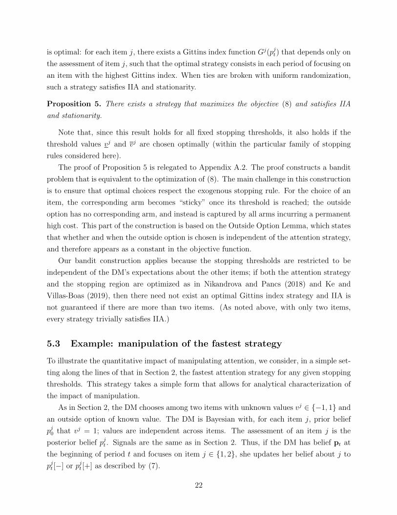
5.3 Example: manipulation of the fastest strategy

To illustrate the quantitative impact of manipulating attention, we consider, in a simple set-

ting along the lines of that in Section 2, the fastest attention strategy for any given stopping

thresholds. This strategy takes a simple form that allows for analytical characterization of

the impact of manipulation.

As in Section 2, the DM chooses among two items with unknown values vj ∈ {−1, 1} and

an outside option of known value. The DM is Bayesian with, for each item j, prior belief

pj0 that vj = 1; values are independent across items. The assessment of an item j is the

posterior belief pjt . Signals are the same as in Section 2. Thus, if the DM has belief pt at

the beginning of period t and focuses on item j ∈ {1, 2}, she updates her belief about j to

pjt [−] or pjt [+] as described by (7).

22

For simplicity, assume that the stopping thresholds p and p are the same for the two items,

and that each of these thresholds can be reached exactly through some sequence of signals.

Thus, the belief process for each item takes realizations in the set {p, p[+], . . . , p[−], p}.

p1|p

|p

p2

−p

−p

•

•

•

•

•

•

•

•

•

•

•

•

•

•

•

•

•

•

•

•

•

•

•

•

•

•

•

•

•

•

•

•

•

•

•

•

•

•

•

•

•

•

•

•

•

•

•

•

•

Item1

chosen

Item 2 chosen

OO chosen

0.07 0.16 0.3 0.5 0.7 0.84 0.93 0.99

0.5

1

p1

D1ea

BA

e1

Figure 2: A: the fastest attention strategy α∗. B: the ex ante demand D1ea(p1, p2) for item 1

as a function of p1. The belief p2 is fixed at 0.7 (solid curve), or 0.3 (dashed curve). Thestopping thresholds are p ≈ .99 and p ≈ .01. The depicted (single-period) manipulationeffect e1 is evaluated for p1 = 0.5, and p2 = .7. The curve for p2 = 0.3 is included forcomparison.

The strategy α∗ depicted in Figure 2A focuses on whichever item the DM views as more

promising. Accordingly, for each item j and j′ 6= j,

α∗j(p) =

1 if pj > pj

′,

1/2 if pj = pj′,

0 otherwise.

(9)

The next result states that α∗ is the fastest attention strategy in this environment. Hence

α∗ is optimal for a DM who, given the stopping region F , minimizes a monotone time cost.14

14Given the stopping rule in this example, minimizing the total expected time cost is equivalent to maxi-mizing the value U(α) in (8) when c (pιtt , ιt) is constant. This equivalence follows from the commonality ofthe thresholds across items together with the Outside Option Lemma.

23

To state this formally, define the (ex ante) stochastic stopping time τ ea(α) for strategy α to

be the minimal time t at which pt(α) ∈ F under the ex ante law P eaα = EP v

α .

Proposition 6. For any strategy α, τ ea(α) first-order stochastically dominates τ ea(α∗).

As with our main results, the proof of this result in Appendix A.2 makes use of coupling,

although the particular construction is distinct from our main one. A different coupling

construction is necessary because the strategy α∗ is not the fastest one in every learning draw:

there exist draws in which focusing on the more promising item leads to a long sequence of

contradictory signals. To prove Proposition 6, we construct a distinct probability space in

which a learning process generated by any strategy α follows the ex ante law P eaα , and α∗ is

always at least as fast as any other strategy.

How much does the manipulation of attention affect demand? To quantify the effect,

define the ex ante demand for j by

Djea(p0) = P ea

α∗

(pτ ∈ F j

)= Ep0 D

j(v;α∗).

Thus Djea(p0) is the ex ante probability that a DM with prior belief p0 chooses item j under

the fastest strategy α∗. Given a prior belief p, we define the manipulation effect ei(p) to be

the change in the ex ante demand for i resulting from a single-period manipulation of the

fastest strategy α∗ that targets the item i; that is,

ei(p) = E[Di(v;µ)−Di(v, α∗)

]= EDi

ea

(pi, p−i

)−Di

ea(pi, p−i), (10)

where the first expectation is with respect to v distributed according to the prior p, µ is the

manipulated strategy that focuses on item i in the first period and follows α∗ thereafter, pi

is the belief resulting from a single-period update of pi, and the second expectation is over

the possible values pi[+] and pi[−] of pi. The magnitude of the effect is therefore determined

by the curvature of Diea(pi, p−i) with respect to pi around p; see Figure 2B. Note that, by

Proposition 4, ei(p) is nonnegative for all p.

Proposition 7. The manipulation effect ei(p) is

1. positive (i.e., nonzero) whenever manipulation affects attention (i.e. when pi ≤ p−i),

2. decreasing in p−i on {pi[+], . . . , p},

3. increasing in pi on {p, p[+], . . . , p−i[−]}, and

4. nonvanishing as p→ 0 and p→ 1 (in the region where the effect is positive).

24

Proposition 7, which is proved in Appendix A.2, implies that manipulation has the

strongest impact when it targets an item with a small a priori disadvantage relative to

the other item. Equation (18) in the appendix provides an explicit expression for the size of

the manipulation effect.

While the analysis above applies for exogenously fixed stopping beliefs, similar results

hold in a related setting in which the stopping region is chosen optimally when the DM is

patient. Ke and Villas-Boas (2019) examine a continuous-time model with exponential dis-

counting and show that the analogue of the strategy α∗ (together with a stopping region they

characterize) is optimal. Despite the differences between these models, they both converge

to the same demands in the limit as learning becomes arbitrarily precise, i.e., in the limit

as p→ 0 and p→ 1 in our model, and as the discount factor tends to 1 in the model of Ke

and Villas-Boas. Therefore, they both exhibit exactly the same manipulation effect in their

respective limits.

5.4 No outside option: choice by elimination and approval

While our main focus is on choice in the presence of a known outside option, many laboratory

experiments employ a “forced choice” design in which there is no such option and subjects

must eventually choose one of the items. Formally, we model the difference between these

two cases by varying the stopping rule: in the presence of an outside option, the DM chooses

an item only if she is sufficiently convinced that it is good, whereas with no outside option,

she may choose an item simply because she is convinced the others are bad. In this section,

we show that, with no outside option, the direction of the effect of attention manipulation

generally depends on the value of the target item. With binary values and a Bayesian DM, as

stopping thresholds become precise, manipulating attention toward a good item increases its

demand, while manipulating attention toward a bad item has the opposite effect. This result

parallels the experimental findings of Armel et al. (2008) and Milosavljevic et al. (2012), who

manipulate focus in forced-choice problems involving either desirable or aversive items.

In our model of forced choice, the DM selects exactly one item from the set I = {1, . . . , I}.Each item j has value vj ∈ {−1, 1}. The DM learns about these values using an attention

strategy α, with the signal structure and assessments pjt defined as in Section 2. (In particu-

lar, each pjt is a log-likelihood ratio.) Relative to our main model, the decision process differs

in the stopping rule: here, the DM stops and chooses an item if she is sufficiently certain

either that its value is high, or that the values of all other items are low. More precisely, for

each item j, there are thresholds pj and pj. Letting p = (p1, p1, p2, p2, . . . , pI , pI), the DM

25

stops learning and chooses item j whenever p lies in the set

F jno(p) =

{p : pj ≥ pj or pj

′ ≤ pj′

for all j′ 6= j}.

Let Fno(p) =⋃Ij=1 F

jno(p), and define the stopping time τ(α, p) = min{t : pt(α) ∈ Fno(p)};

to simplify notation, we write τ in place of τ(α, p) when the arguments are clear from the

context. As before, we define the interim demand for item j, Dj(v;α, p) = P vα (pτ ∈ F j

no(p)),

to be the probability that j is chosen conditional on the items’ values.

The next result states that, in the limit as learning becomes perfectly precise, manip-

ulating attention increases demand for a high-value target item and decreases demand for

a low-value target item. This result holds for the same class of attention strategies as in

Proposition 4.15 Its proof may be found in Appendix A.2.

Proposition 8. Let pl be a sequence of thresholds such that pil→ −∞ and pil → ∞. Let

(βl, µl) be a sequence of baseline and manipulated strategy pairs, each with target item i, such

that, for each l, βl is stationary and satisfies IIAi, and both βl and µl are non-wasteful with

respect to pl. Then,

lim infl→∞

(Di (v;µl, pl)− Di (v; βl, pl)

)≥ 0 if vi = 1, (11)

and lim supl→∞

(Di (v;µl, pl)− Di (v; βl, pl)

)≤ 0 if vi = −1. (12)

This result demonstrates the importance of the stopping rule in determining the effect of

manipulation. When the stopping rule allows for an item to be chosen because of a negative

signal about a different item, manipulation can, in some cases, reduce demand for the target

item. For example, with two items and no outside option, suppose the thresholds are such

that a single negative signal about either item j is enough for pj to drop below pj. Then, in

any draw that begins with such a signal for each item, the item chosen is whichever one is

not examined in the first period. Therefore, manipulation does not increase demand for the

target item across all draws, thresholds, and attention strategies.

The proof of Proposition 8 (in the appendix) uses the same coupling construction as in

the proof of Proposition 4: the coupling is across learning processes πj that focus exclusively

on items j = 1, . . . , I, respectively. Whenever the learning process for the target item i

reaches its lower threshold pi (before reaching its upper threshold) and the learning process

15Proposition 8 does not generally hold outside of the limit. For a counterexample, consider a binary choicewith a baseline attention strategy that focuses on item 2 whenever it is not excluded by the non-wastefulnesscondition. Suppose v1 = −1. Manipulation that induces the DM to focus on item 1 in the first periodand return to the baseline strategy thereafter increases demand for item 1 if there is some chance that theassessment p1 reaches p1 following a single inspection.

26

for at least one other item j 6= i reaches its upper threshold pj, no attention strategy leads

to item i being chosen. Hence choice is manipulable only if (i) the learning process πi for the

target item reaches its upper threshold, or (ii) the learning processes for all items reach their

lower thresholds. As the lower threshold for item i approaches −∞ and its upper threshold

approaches ∞, the probability of event (i) vanishes when the value of i is low and, likewise,

the probability of event (ii) vanishes when its value is high. Finally, the manipulation effect

is nonnegative in all draws in (i), and nonpositive in all draws in (ii).

The presence of an outside option affects demand in two distinct ways: directly, by

allowing the DM not to choose any item, and indirectly, by affecting the stopping rule. It

turns out that the direct channel is irrelevant for the manipulation effect: the difference

between the two settings is driven by the stopping rule.

To disentangle the two effects, consider an alternative model in which there is no outside

option, and the stopping rule is that from our main setting. Thus learning stops with the

choice of item j whenever pτ ∈ F j = {p : pj ≥ pj} for some j, and with an equal probability

of choosing any item whenever pτ ∈ F oo = {p : pj ≤ pj for all j}. The demand for item j is

therefore

Djalt(v;α) = P v

α

(pτ ∈ F j

)+

1

IP vα (pτ ∈ F oo)

= Dj(v;α) +1

|I|Doo(v;α), (13)

where Dj(v;α) is the interim demand for j ∈ I∪{oo} from our main setting with an outside

option. By the Outside Option Lemma, the second summand in (13) is independent of the

attention strategy. It follows that

Djalt(v;µ)−Dj

alt(v; β) = Dj(v;µ)−Dj(v; β),

and thus, for each v, the manipulation effect in this alternative model is the same as in our

main model with an outside option; the presence of the outside option affects the impact of

manipulation only through the stopping region.

A similar argument applies if the threshold for stopping and accepting an item depends

on the assessments of other items. For example, in the Bayesian continuous-time model

analyzed by Ke and Villas-Boas (2019), the threshold for accepting an item is increasing in

the belief about the other item (in the case of two items). At a prior lying just to the right of

the threshold for accepting item 2, manipulating attention toward item 1 can have a negative

effect on demand in draws that initially feature negative information about both items. In

their solution, when the value of the outside option is low, there is a large range of beliefs

27

at which an item is chosen immediately when the other is eliminated. For higher values of

the outside option, for many beliefs, when one item is eliminated, the DM continues to learn

about the other one, as in our model.

6 Further applications

6.1 Clinical trials

One setting outside of marketing in which manipulation may be of concern is clinical trials

(Gallo et al., 2006). Adaptive designs, in which the assignment of treatments depends on

their success so far, are becoming increasing popular in phase II clinical trials (Berry, 2006).

In a “drop-the-loser” design, treatments that perform poorly are eliminated before the end

of the trial. Similarly, those that perform well may be approved for phase III before the trial

ends. In keeping with regulatory requirements, success or failure is typically judged based

on a fixed level of statistical significance, as in the fixed thresholds in our model.16

We analyze the effect of manipulation in the administration of treatments in a stylized

model of adaptive clinical trials. A laboratory runs a sequential trial of a finite set I of I

different drugs on at most T patients, where T is predetermined. In each period t = 1, . . . , T ,

a new patient arrives and is administered a drug ιt ∈ I, the effect xt of which is observed.

The distribution of xt depends on the unknown quality of the administered drug and on

random unobservable characteristics of the patient. Starting from an initial score pj0 for each

drug j, the score pιtt ∈ R for drug ιt is updated to pιtt+1 = φ (pιtt , xt) according to a discrete

transition map φ, while the scores of the remaining drugs j 6= ιt are kept unchanged.

The choice of drug to administer to each patient is governed by a baseline strategy

β : RI −→ ∆(I). A drug is dropped from the trial and not administered again once its

score falls below a fixed threshold pi; that is, βj(p, t) = 0 for all p such that pj ≤ pj. A

drug is approved (for production or more advanced testing) once its score exceeds a fixed

threshold pj. Several drugs can be approved. An approved drug is not tested further within

the trial: βj(p, t) = 0 for all p such that pj ≥ pj. The trial terminates at some time τ once

every drug has been either dropped or approved, or all T patients have participated. Let

Dj(v;α) = P vα

(pjτ (α) ≥ pj

)be the probability that j is approved under strategy α.

Corollary 2. Suppose the baseline strategy β is stationary and satisfies IIAi, and let µ

be a manipulated strategy with target i. Manipulation weakly increases the probability that

16Adaptive designs of clinical trials are increasingly popular both because of their statistical advantagesand because of ethical concerns related to administration of drugs that, based on evidence accumulatedduring the trial, appear to be inferior. Termination rules are often set in accordance with simple statisticalsignificance cutoffs imposed by regulatory bodies or by academic journals. See Berry (2006) for an overview.

28

the target drug is approved and weakly decreases the approval probability of the other drugs:

Di(v;µ) ≥ Di(v; β) and Dj(v; β) ≥ Dj(v;µ) for all j 6= i.

One example of a stationary strategy that satisfies IIA and may be ethically appealing is

the one that always administers the drug having the highest current score (among those that

have not already been approved). A simple form of manipulation consists of administering

the target drug to the first m patients and then continuing with the baseline strategy β.

The result is a corollary of the Attention Theorem. Since, by any period t, the target

drug receives at least as much cumulative attention—i.e., is administered at least as many

times—under the manipulated strategy as under the baseline strategy, it is approved under

µ in any draw in which it is approved under β. Similarly, for any other drug, in any draw for

which it is approved under the manipulated strategy, it is also approved under the baseline

strategy.

6.2 A neuroeconomic model of choice

The fixed thresholds in our one-shot choice model differ from those in the optimal strategy

in Ke and Villas-Boas (2019), which features thresholds for acceptance that are increasing in

the belief about the other item. A related (but distinct) implementation of varying standards

for acceptance appears in neuroscience in the form of so-called “inhibitory links.” Signals

favoring the choice of each option are accumulated in distinct brain areas called “accumu-

lators”; a given option is chosen once the firing rate of its associated accumulator exceeds

a fixed threshold (Shadlen and Newsome, 2001). When a stimulus causes the accumulator

associated with one item to increase, the accumulator for the other item is inhibited via the

inhibitory links (see, e.g., Sterling and Laughlin, 2015).

We model the decision process from Shadlen and Newsome (2001) as follows. The DM

chooses one of two items j = 1, 2 with values vj ∈ {−1, 1}. In each period t = 0, 1, . . . ,

she inspects an item, ιt. If the inspected item is good (i.e., vιt = 1), then she receives a

stimulus with probability λ > 1/2; if it is bad, she receives a stimulus with probability 1−λ.

Receipt of a stimulus for an item increases the accumulator for that item and inhibits the

accumulator for the other item. More precisely, the value of the accumulator for item j = 1, 2

at the beginning of period t is

pjt =∑

s<t:ιs=j

xs − χ∑

s<t:ιs=j′

xs,

where j′ 6= j, xs ∈ {0, 1} is an indicator of whether the DM received a stimulus in period s,

and χ > 0 is a parameter governing the strength of inhibition.

29

Inspection is determined by an arbitrary baseline attention strategy β, which is a function

of the pair pt = (p1t , p

2t ). There is a fixed threshold pj for each j such that the process

terminates with the choice of item j as soon as pjt ≥ pj. (If neither accumulator reaches the

threshold, the DM never makes a choice.) Let F j = {p : pj ≥ pj}, τ = mint{pt ∈ F 1 ∪ F 2},and Dj(v;α) = P v

α (pτ ∈ F j).

Corollary 3. Suppose the baseline strategy β is stationary, and let µ be a manipulated

strategy. Manipulation weakly increases the probability that the target item is chosen and

weakly decreases the probability that the other item is chosen; that is, Di(v;µ) ≥ Di(v; β)

for the target item i, and Dj(v; β) ≥ Dj(v;µ) for j 6= i.

As stated, this model is not a special case of our main model because the assessment

pjt of item j can change when the other item is inspected. However, a simple reformulation

enables us to apply the Attention Theorem (of which it is a corollary). Let qjt =∑

s<t:ιs=j xs,

β (q1t , q

2t ) = β (q1

t − χq2t , q

2t − χq1

t ), µ (q1t , q

2t ) = µ (q1

t − χq2t , q

2t − χq1

t ), and the stopping region

be F j ={q : qjt − χq

−jt ≥ p

}for each j. With this reformulation, each assessment qjt depends

only on the stimuli for item j, and the Attention Theorem applies. It follows that the

cumulative attention k(i, t, µ) devoted to the target item i under the manipulated strategy,

µ, is always at least as large as that under the baseline strategy, β, and the opposite is

true for the other item, j. In our coupling construction, in every draw, qit(µ) ≥ qit(β) and

qjt (β) ≥ qjt (µ) for each t because, in this model, the assessment of an item is nondecreasing

in the number of periods of focus on that item. Therefore,

pit(µ) = qit(µ)− χqjt (µ) ≥ qit(β)− χqjt (β) = pit(β)

and

pjt(β) = qjt (β)− χqit(β) ≥ qjt (µ)− χqit(µ) = pjt(µ)

for each t and each draw. The first claim in the corollary now follows: for each draw in

which strategy β terminates with the choice of i, so does strategy µ. The argument for the

second claim is similar.

7 Summary and discussion

We show how manipulating attention toward an item can boost a DM’s demand for it.

Our argument has two key parts. The first is to identify the effect of manipulation on the

cumulative attention paid to an item. While manipulation has the direct effect of increasing

attention to the target item, it also affects attention indirectly through the DM’s subsequent

30

choices of which item to focus on. We show that, under general conditions on the DM’s

strategy, this indirect effect never overcomes the direct effect, and therefore manipulation

can only increase the attention paid to its target. The second part of the argument connects

cumulative attention to choice. With repeated choice, such as multi-armed bandits, this

connection is immediate. In one-shot choice, we show that, in the presence of an outside

option, increased attention implies increased demand when the DM chooses according to a

simple satisficing rule.

Our model offers a novel combination of satisficing and gradual learning about the values

of available choices. This combination necessitates some differences compared to standard

models of satisficing behavior. Most notably, with gradual learning, one must take a stand

on whether and when the DM rejects an item and stops learning about it. We assume that

rejection occurs when the assessment falls below a fixed threshold, just as acceptance is

associated with exceeding a fixed threshold.

The positive effect of attention manipulation can break down in one-shot choice if the

DM sometimes chooses by elimination, i.e., as a result of rejecting other items without first

verifying the value of the chosen item. Choice by elimination arises naturally in the absence

of an outside option, or if the DM optimizes her stopping rule instead of satisficing. For

optimal stopping by a Bayesian DM, while we know that our main result does not generally

hold as stated—i.e., for every prior and realized profile of values, and a large class of attention

strategies—identifying the parameters of the model for which it does is an open question.

References

Armel, K. C., A. Beaumel, and A. Rangel (2008). Biasing simple choices by manipulating

relative visual attention. Judgment and Decision Making 3 (5), 396–403.

Atalay, A. S., H. O. Bodur, and D. Rasolofoarison (2012). Shining in the center: Central

gaze cascade effect on product choice. Journal of Consumer Research 39 (4), 848–866.

Austen-Smith, D. and C. Martinelli (2018). Optimal exploration. Working paper.

Bagwell, K. (2007). The economic analysis of advertising. In M. Armstrong and R. Porter

(Eds.), Handbook of Industrial Organization, Volume 3, pp. 1701–1844. Elsevier.

Becker, G. S. and K. M. Murphy (1993). A simple theory of advertising as a good or bad.

Quarterly Journal of Economics 108 (4), 941–964.

Berry, D. A. (2006). Bayesian clinical trials. Nature Reviews Drug Discovery 5 (1), 27–36.

31

Bogacz, R., E. Brown, J. Moehlis, P. Holmes, and J. D. Cohen (2006). The physics of

optimal decision making: a formal analysis of models of performance in two-alternative

forced-choice tasks. Psychological Review 113 (4), 700.

Braithwaite, D. (1928). The economic effects of advertisement. The Economic Jour-

nal 38 (149), 16–37.

Chandon, P., J. W. Hutchinson, E. T. Bradlow, and S. H. Young (2009). Does in-store

marketing work? Effects of the number and position of shelf facings on brand attention

and evaluation at the point of purchase. Journal of Marketing 73 (6), 1–17.

Che, Y.-K. and K. Mierendorff (2019). Optimal dynamic allocation of attention. American

Economic Review 108 (8), 2993–3029.

Chernoff, H. (1959). Sequential design of experiments. Annals of Mathematical Statis-

tics 30 (3), 755–770.

Dukas, R. (2002). Behavioural and ecological consequences of limited attention. Philosophical

Transactions of the Royal Society of London B: Biological Sciences 357 (1427), 1539–1547.

Eliaz, K. and R. Spiegler (2011). On the strategic use of attention grabbers. Theoretical

Economics 6 (1), 127–155.

Fogg-Meade, E. (1901). The place of advertising in modern business. Journal of Political

Economy 9 (2), 218–242.

Gallo, P., C. Chuang-Stein, V. Dragalin, B. Gaydos, M. Krams, and J. Pinheiro (2006).

Adaptive designs in clinical drug development: an executive summary of the PhRMA

working group. Journal of Biopharmaceutical Statistics 16 (3), 275–283.

Gasmi, F., J. J. Laffont, and Q. Vuong (1992). Econometric analysis of collusive behavior

in a soft-drink market. Journal of Economics & Management Strategy 1 (2), 277–311.

Gittins, J. and D. Jones (1974). A dynamic allocation index for the sequential design of

experiments. In J. Gani (Ed.), Progress in Statistics, pp. 241–266. Amsterdam, NL: North-

Holland.

Kaldor, N. (1950). The economic aspects of advertising. Review of Economic Studies 18 (1),

1–27.

Ke, T. T., Z.-J. M. Shen, and J. M. Villas-Boas (2016). Search for information on multiple

products. Management Science 62 (12), 3576–3603.

32

Ke, T. T. and J. M. Villas-Boas (2019). Optimal learning before choice. Journal of Economic

Theory 180, 383–437.

Krajbich, I., C. Armel, and A. Rangel (2010). Visual fixations and the computation and

comparison of value in simple choice. Nature Neuroscience 13 (10), 1292.

Krajbich, I. and A. Rangel (2011). Multialternative drift-diffusion model predicts the rela-

tionship between visual fixations and choice in value-based decisions. Proceedings of the

National Academy of Sciences 108 (33), 13852–13857.

Lindvall, T. (1992). Lectures on the Coupling Method. Wiley.

Lou, D. (2014). Attracting investor attention through advertising. Review of Financial

Studies 27 (6), 1797–1829.

Mandelbaum, A., L. A. Shepp, and R. J. Vanderbei (1990). Optimal switching between a

pair of Brownian motions. Annals of Probability 18 (3), 1010–1033.

Mayer, A. R., J. M. Dorflinger, S. M. Rao, and M. Seidenberg (2004). Neural networks

underlying endogenous and exogenous visual-spatial orienting. Neuroimage 23 (2), 534–

541.

Milosavljevic, M., V. Navalpakkam, C. Koch, and A. Rangel (2012). Relative visual saliency

differences induce sizable bias in consumer choice. Journal of Consumer Psychology 22 (1),

67–74.

Nelson, P. (1974). Advertising as information. Journal of Political Economy 82 (4), 729–754.

Nikandrova, A. and R. Pancs (2018). Dynamic project selection. Theoretical Eco-

nomics 13 (1), 115–143.

Orquin, J. L. and S. M. Loose (2013). Attention and choice: A review on eye movements in

decision making. Acta Psychologica 144 (1), 190–206.

Platt, M. L. and P. W. Glimcher (1999). Neural correlates of decision variables in parietal

cortex. Nature 400 (6741), 233.

Ratcliff, R. (1978). A theory of memory retrieval. Psychological Review 85 (2), 59.

Seasholes, M. S. and G. Wu (2007). Predictable behavior, profits, and attention. Journal of

Empirical Finance 14 (5), 590–610.

33

Shadlen, M. N. and W. T. Newsome (2001). Neural basis of a perceptual decision in the

parietal cortex (area lip) of the rhesus monkey. Journal of Neurophysiology 86 (4), 1916–

1936.

Simon, H. A. (1955). A behavioral model of rational choice. Quarterly Journal of Eco-

nomics 69 (1), 99–118.

Spelke, E., W. Hirst, and U. Neisser (1976). Skills of divided attention. Cognition 4 (3),

215–230.

Sterling, P. and S. Laughlin (2015). Principles of Neural Design. MIT Press.

Stigler, G. J. (1961). The economics of information. Journal of Political Economy 69 (3),

213–225.

Stigler, G. J. and G. S. Becker (1977). De gustibus non est disputandum. American Economic

Review 67 (2), 76–90.

Telser, L. G. (1964). Advertising and competition. Journal of Political Economy 72 (6),

537–562.

Tsitsiklis, J. N. (1994). A short proof of the gittins index theorem. Annals of Applied

Probability 4 (1), 194–199.

Wald, A. (1945). Sequential tests of statistical hypotheses. Annals of Mathematical Statis-

tics 16 (2), 117–186.

Weber, R. (1992). On the Gittins index for multiarmed bandits. Annals of Applied Proba-

bility 2 (4), 1024–1033.

Yorzinski, J. L., G. L. Patricelli, J. S. Babcock, J. M. Pearson, and M. L. Platt (2013).

Through their eyes: Selective attention in peahens during courtship. Journal of Experi-

mental Biology 216 (16), 3035–3046.

34

Appendix

A Proofs

A.1 Proofs for Section 3

We consider a baseline strategy β and a manipulated strategy µ in favour of item i.

The main difficulty compared to the construction of the probability space in Section 3.1

is that the strategies β and µ are stochastic instead of deterministic. This requires us to

amend our coupling construction in order to keep track of the realized items of focus. We

thus use the learning process π = (πj)Ij=1 as constructed in Section 3.1, and introduce an

attention process consisting of random variables (ap,t)p,t, (bp−i,t)p−i,t, and (cp,t)p,t, all of

which are independent and are independent of the learning process. The random variable

ap,t takes values in {0, 1} and Pr(ap,t = 1) = µi(p, t). The random variable bp−i,t takes

values in I \ {i}. For a fixed value of p−i, if there exists pi such that βi(pi,p−i) 6= 1, then

the probability that bp−i,t takes the value j 6= i is βj (pi,p−i) /(1− βi (pi,p−i)), where we

note that the particular value of pi in the formula is irrelevant since β satisfies IIAi.17 The

random variable cp,t takes values in {0, 1} and Pr(cp,t = 1) = βi(p)µi(p,t)

whenever µi(p, t) > 0

(and is otherwise arbitrary). A realization of the attention process is called an attention

draw. We refer to a pair of learning and attention draws simply as a draw.

For a strategy α = β or µ, we recursively construct the processes (pt(α), ιt(α))t as

functions of the draw. Recall that k(j, t;α) denotes the cumulative focus on item j up to

period t − 1 given by the realizations (ιt(α))1, . . . , ιt(α))t−1). We let pjt(α) = πjk(j,t;α) be

the belief about item j after k(j, t;α) inspections. We proceed to construct the focus ιt(α)

whenever pt /∈ F . Given a sequence of assessments and focus items (ps(α), ιs(α))s<t and

any vector p−i of assessments about items j 6= i, we let ν (p−i, t;α) be the total number of

periods before time t with assessments p−i about items j 6= i in which the DM does not

focus on the target item i; that is,

ν(p−i, t;α) = |{s < t : p−is (α) = p−i, ιs(α) 6= i}|.

For the strategy µ, let ιt(µ) = i if apt(µ),t = 1 and ιt(µ) = bp−it (µ),ν(p−i

t (µ),t;µ) otherwise. For

the strategy β, let ιt(β) = i if apt(β),tcpt(β),t = 1 and ιt(β) = bp−it (β),ν(p−i

t (β),t;β) otherwise.

By construction, conditional on (p0(α), ι0(α), . . . ,pt−1(α), ιt−1(α),pt(α)), ιt(α) is dis-

tributed according to α(pt(α), t). Conditional on (p0(α), ι0(α), . . . ,pt(α), ιt(α)), pjt+1(α) =

17The specification of bp−i,t when no such pi exists is immaterial for our purposes.

35

pjt(α) for all j 6= ιt(α), and pιt(α)t+1 (α) is distributed according to φιt(α)

(pιt(α)t (α), vιt(α)

). There-

fore, the law of the process (pt(α), ιt(α))t is P vα for both α = β, µ, and this is indeed a valid

coupling.

Let k(−i, t;α) = t − k(i, t;α) denote the number of periods of focus on items other

than the target i. To simplify notation, let k(j, t) = k(j, t; β) and k(j, t) = k(j, t;µ) for

j ∈ I ∪ {−i}. For any n ≥ 0, let t(n) be the n-th period such that ιt 6= i under the baseline

strategy; that is, t(n) = min{t : k(−i, t) ≥ n} (where potentially t(n) = ∞). Similarly, let

t(n) = min{t : k(−i, t) ≥ n}. Let (pt, ιt)t = (pt(β), ιt(β))t and (pt, ιt)t = (pt(µ), ιt(µ))t.

Lemma 2 (Coupling Lemma). The baseline and manipulated processes coincide when re-

stricted to periods of focus on items other than the target, i. That is, for every n such that

t(n), t(n) <∞, (p−it(0), ιt(0), . . . ,p

−it(n), ιt(n)

)=(p−it(0), ιt(0), . . . , p

−it(n), ιt(n)

).

Proof of the Coupling Lemma. We prove the result by induction. The property holds for

n = 0 since p−it(0) = p−it(0)

= p−i0 . Assume it holds for n. For item j = ιt(n) = ιt(n), we have

pjt(n+1) = πjk(j,t(n))+1 = πjk(j,t(n))+1

= pjt(n+1)

. For items j 6= i, ιt(n) that do not receive attention

in periods t(n) and t(n), respectively, we have pjt(n+1) = pjt(n) = pjt(n) = pjt(n+1)

. Thus we have

p−it(n+1) = p−it(n+1)

.

It remains to show that the items of attention in period t(n+ 1) of the baseline process

and in period t(n+1) of the manipulated process coincide. By the definitions of the attention

processes, we have

ιt(n+1) = bp−it(n+1)

,ν(p−it(n+1)

,t(n+1)) = b

p−i

t(n+1),ν(p−i

t(n+1),t(n+1)

) = bp−i

t(n+1),ν(p−i

t(n+1),t(n+1)

) = ιt(n+1)

since, by the induction hypothesis, ν(p−it(n+1), t(n+ 1)) = ν(p−it(n+1)

, t(n+ 1)).

Proof of the Attention Theorem. We prove by induction that k(i, t) ≥ k(i, t) and k(−i, t) ≤k(−i, t) for all periods t. This statement obviously holds for period t+ 1 if k(i, t) > k(i, t).

Suppose that k(i, t) = k(i, t) in period t. By the Coupling Lemma,(p−it(0), ιt(0) . . . ,p

−it(k(−i,t)), ιt(k(−i,t))

)=(p−it(0), ιt(0), . . . , p

−it(k(−i,t)), ιt(k(−i,t))

).

Therefore, for every j ∈ I, k(j, t) = k(j, t), so that the cumulative focus on each item

before time t is the same in the two processes, which implies that pt = pt. By the coupling

construction, for each p and t, the baseline process focuses on the target item i at time t

36

only if the manipulated process focuses on i at t. Thus, again, the statement holds in period

t+ 1.

Additionally, the Coupling Lemma implies that items j 6= i are explored in the same order

under both processes, which in turn implies that, for every t and every j 6= i, k(j, t) ≤ k(j, t),

as needed.

A.2 Proofs for Section 5

The next two proofs use the probability space arising from the coupling construction in

Section A.1.

Proof of the Outside Option Lemma. Fix a learning draw such that τ oo(α) is finite; that is,

strategy α leads to the outside option being chosen. For each item j, let κj = min{κ : πjκ ≤pj} be the number of steps needed for the learning process πj to reach the threshold pj.

Since α stops with the choice of the outside option once all beliefs reach their respective

lower thresholds, τ oo(α) =∑

j κj, which is independent of α. In particular, the distribution

of τ oo(α), as well as whether the outside option is chosen (i.e., τ oo(α) <∞), are independent

of α, and so is the probability of this event.

Proof of Proposition 4, inequality (5). Consider any draw such that, under the manipulated

process, an item j 6= i is chosen in period τ . Then, by the Outside Option Lemma, the

baseline process does not choose the outside option. Suppose for contradiction that, under

the baseline process, the target item i is chosen in some period τ ≤ τ . Then piτ ≥ pi. By

the Attention Theorem, there exists a period t ≤ τ such pit = piτ ≥ pi and hence under

the manipulated process, i is chosen in period t ≤ τ , which establishes the contradiction.

Therefore, it cannot be that, under the baseline process, i or the outside option is chosen

at a time τ ≤ τ . By the Attention Theorem, k(−i, t) ≥ k(−i, t) for all t. By the Coupling

Lemma, the beliefs p−i and p−i coincide when restricted to the periods of focus on items

−i. Hence, there exists τ ≤ τ such that p−iτ = p−iτ , and the baseline process stops in period

τ with the choice of item j, as needed.

Proof of Proposition 5. We construct a bandit problem and apply a result from Tsitsiklis

(1994) showing the existence of an optimal (stationary) Gittins index strategy; with an

appropriate choice of tie-breaking rule, such strategies satisfy IIA. In the model of Tsitsiklis

(1994) (described in the language of our model), when the DM selects an item j = ιt with

belief pjt in period t, she receives a stochastic flow reward R(pjt , j) and the selected item

remains active for T j(pjt) periods. In period t + T j(pjt), the belief about item j transitions

to a new belief pjt+T j(pjt )

= ψj(pjt) according to some stochastic function ψj, while the beliefs

37

about all other items remain unchanged (that is, pj′

t+T j(pjt )= pj

′

t for all j′ 6= j). Then, the

DM selects a new item ιt+T j(pjt ) in period t+ T j(pjt), and so on. . . Let tk denote the random

sequence of periods in which the DM selects items: t0 = 0 and tk+1 = tk + T (pιtktk

) for each

k ≥ 0. The DM’s problem is to maximize the expected discounted total reward:

Γ(α) = E∞∑k=0

δtkR(pιtktk, ιtk). (14)

Let φj(pjt+1 | p

jt

)denote the ex ante Markov transition probabilities of the DM’s belief

about item j when she focuses on j in period t, and define the stochastic transition function

ψj by Pr(ψ(pjt) = p

)= φj

(p | pjt

)for each p. Fix the reward function to be

R (p, j) =

−c (p, j) if vj < E [vj | pj = ψj(p)] < vj,

−c (p, j) + E [vj | pj = ψj(p)] if E [vj | pj = ψj(p)] ≥ vj,

−c otherwise,

where c is a uniform upper bound on c (pιtt , ιt). If item j is selected in period tk, we set the

activity length T j(pjtk) to be 1 if E[vj | pjtk+1

]< vj and ∞ otherwise.18

This problem differs from the original problem (8) in that the flow payoff from focusing

on item j in period t depends only on pjt and is independent of pj′

t for j′ 6= j. The flow

payoffs in the original problem are interdependent because whether the DM stops upon her

expectation of vj reaching vj depends on whether expectations for other items have reached

their respective thresholds. This difference allows us to apply Theorem 2.2 from Tsitsiklis

(1994) (see also Weber, 1992): an optimal solution to the bandit problem (14) is a Gittins

index strategy where the index for an item depends only on the current belief about the item.

In particular, when ties for the highest Gittins index are broken by uniform randomization,

this describes an optimal strategy that satisfies IIA and stationarity.

It remains to connect the bandit problem (14) to the original problem (8). Note that any

optimal strategy in the bandit problem (i) chooses an item j forever once E[vj | pjt

]≥ vj,

and (ii) always chooses an item j such that E[vj | pjt

]> vj provided such an item exists.

Note that Γ(α) = U(α) − cE∑∞

t=1 1t≥τoo(α), where the expectation is with respect to

τ oo(α). By the Outside Option Lemma, τ oo(α) is identical for all α satisfying (i) and (ii).

Therefore, there exists a constant Kδ such that

Γ(α) = U(α) +Kδ. (15)

18This correlation among the active-period length, reward, and assessment transition complies with Tsit-siklis’s setting, as he allows for arbitrary correlations among these random variables.

38

Thus, a non-wasteful strategy α solves the auxiliary bandit problem (14) if and only if it

solves the original problem (8), as needed.

Proof of Proposition 6. This proof makes use of coupling: we construct a common probabil-

ity space on which we can compare the processes of beliefs pt(α) across attention strategies

α. However, the idea of the proof and the construction of the probability space significantly

differ from that in the proof of Proposition 4.

In this construction, an outcome in the probability space specifies, for every possible

belief, the sequence of belief transitions on any of the items starting at this belief. Let

Π = {p[+], p[+][+], . . . , p[−][−], p[−]} denote the set of beliefs that the DM may attain for

either item. For each π ∈ Π and κ = 0, 1, . . ., let (`(π, κ))π,κ be an i.i.d. family of random

variables with values in {π[+], π[−]} such that the respective probabilities that `(π, κ) takes

each value are π−π[−]π[+]−π[−]

and π[+]−ππ[+]−π[−]

. An element of the probability space, which we refer

to as an updating draw, is a realization of the family of random variables (`(π, κ))π,κ. We

interpret `(π, κ) as the updated belief of a DM who learns for one period about an item

j = 1, 2 starting at the belief pj = π, where κ indicates the total number of times the DM

has focused on an item with associated belief π earlier on.

We now construct, for each fixed updating draw and any attention strategy α, the process

of beliefs pt(α) and verify that they follow the law P eaα . Let kt(α) = (kπt (α))π∈Π be an

auxiliary counter that takes values in N|Π|. We interpret kπt (α) as the number of times the

belief π has been updated up to period t under strategy α. Define the joint process of the

beliefs pt(α) and the counter kt(α) as follows. Let kπ0 (α) = 0 for all π and p0(α) = p0. In

each period t, the focus of attention ιt is chosen according to the attention strategy α(pt, t).

Recursively define

kπt+1(α) =

kπt (α) + 1 if π = pιtt ,

kπt (α) otherwise

and

pjt+1(α) =

`(π, k

pjt (α)t (α)

)if j = ιt,

pjt(α) otherwise.

By construction, for each strategy α, the beliefs pt(α) follow the law P eaα .

We make use of an auxiliary process of the beliefs that would result from learning about a

single item in all periods starting from a prior belief π. This process consists of beliefs at(π)

and a counter hπt for each π, π ∈ Π. Formally, let a0(π) = π and hπ0 = 0 for all π, π ∈ Π, and

39

recursively define at+1(π) = `(at(π), h

at(π)t

), and, for each π ∈ Π,

hπt+1 =

hπt + 1 if π = at(π),

hπt otherwise.

That is, at(π) is the belief in period t and hπt counts how many times belief π has been

updated up to period t in this auxiliary process.

It is convenient to reformulate the stopping rule as follows. For each strategy α, let

Mt(α) = maxj=1,2 pjt(α), M t(α) = maxs=0,...,tMs(α), and M t(α) = mins=0,...,tMs(α). The

strategy α stops by period t, i.e., τ ea(α) ≤ t, if

p = M t(α) or M t(α) = p.

We now prove that, for every prior, in each updating draw, if a strategy α stops by t,

then the strategy α∗ also stops by t. We proceed by induction on t. First, consider t = 1.

The statement is trivial if p10 = p2

0; accordingly, assume p10 6= p2

0. Again, the statement is

trivial if α focuses on the item with the higher belief in period 0; accordingly, assume that α

focuses on the item with the lower belief in period 0. Then M0(α) = M0(α∗) = max{p10, p

20}

and M1(α∗) = a1 (max{p10, p

20}) while M1(α) = max{p1

0, p20}. Thus

M1(α∗) ≤M1(α) ≤M1(α) ≤M1(α∗),

as needed.

Suppose the statement holds for t − 1. If α stops by period t then, since the induction

hypothesis applies regardless of the prior, the strategy α stops by t, where α(p, 0) = α(p, 0)

and α(p, t) = α∗(p) for t > 0. Therefore, to close the induction step, it suffices to prove

that if α stops by t then α∗ stops by t. This is immediate if p10 = p2

0. Accordingly, suppose

that p10 6= p2

0 and, without loss of generality, take p10 < p2

0. If α focuses on item 2 in period

0, then the belief processes are the same under α and α∗. Therefore, let α focus on item 1

in the first period and follow α∗ thereafter.

To compare α and α∗, we distinguish two sets of updating draws. The first set consists of

those for which as(p20) > p1

0 in every period s = 0, 1, . . . , t− 1. For any (ordered) belief pair

p = (p1, p2), write 〈p〉 for the unordered pair {p1, p2}. (By considering the unordered pairs

of beliefs we eliminate the need to keep track of which item has the higher belief and which

is randomly chosen at a tie.) For each updating draw in this first set, for each s = 1, 2, . . . , t,

〈ps(α∗)〉 ={p1

0, as(p2

0

)}and Ms(α

∗) = as(p2

0

),

40

and

〈ps(α)〉 ={a1

(p1

0

), as−1

(p2

0

)}and Ms(α) = as−1

(p2

0

)since as(p

20) > p1

0 and as(p20) ≥ a1(p1

0) for all s = 1, 2, . . . , t − 1. Therefore, α∗ updates

the belief as(p20) in all periods s = 0, . . . , t, and α updates the belief as−1(p2

0) in all periods

s = 1, . . . , t. Thus, for each updating draw in this first set,

M t(α∗) ≤M t(α) ≤M t(α) ≤M t(α

∗),

and the induction step holds.

The second set is the complementary set to the first; that is, it is the set of updating

draws for which there exists a period s ∈ {1, 2, . . . , t − 1} in which as(p20) = p1

0. Let s∗ be

the minimal such period. For each draw in this second set, we have

〈ps∗+1(α∗)〉 ={p1

0, a1(p10)}

since 〈ps∗(α∗)〉 = {p10, p

10} and the belief p1

0 is updated once by s∗ under the strategy α∗. We

also have

〈ps∗+1(α)〉 ={a1(p1

0), as∗(p20)}

since the belief p10 is updated once in period 0 and in each period s = 1, . . . , s∗, 〈ps(α)〉 =

{a1(p10), as−1(p2

0)} and as−1(p20) ≥ a1(p1

0). Thus, the strategy α updates the belief as−1(p20) in

all periods s = 1, . . . , s∗. Since as∗(p20) = p1

0, we have

〈ps∗+1(α)〉 ={a1(p1

0), p10

}= 〈ps∗+1(α∗)〉 .

Therefore, in each updating draw from the second set, 〈ps(α∗)〉 = 〈ps(α)〉 for all s ≥ s∗+ 1.

In particular, α∗ and α stop in the same period, concluding the proof of the induction

step.

Proof of Proposition 7. Without loss of generality, we prove the statements for i = 1. We

claim that

D1ea(p) =

p−p1

2(p−p2)

(1− (p−p2)2

(p−p)2

)+ p1−p2

p−p2 if p1 ≥ p2,

p−p22(p−p1)

(1− (p−p1)2

(p−p)2

)if p1 ≤ p2.

(16)

If p10 = p2

0 = p, then α∗ stops with beliefs (p1τ , p

2τ ) = (p, p) (in which case the outside option

is chosen) with probability(p−pp−p

)2

. By symmetry, for p10 = p2

0, conditional on not choosing

41

the outside option, the DM chooses item 1 with probability 1/2. Thus

D1ea(p, p) =

1

2

(1−

(p− pp− p

)2). (17)

Now consider prior beliefs such that p10 > p2

0. The strategy α∗ initially focuses on item 1

until p1t = p or p1

t = p20. In the former case, which occurs with probability

p10−p20p−p20

, the DM

chooses item 1. In the latter case, which occurs with probabilityp−p10p−p20

, the DM chooses item

1 with probability D1ea(p2

0, p20). Therefore, for p1 > p2,

D1ea(p1, p2) =

p1 − p2

p− p2+p− p1

p− p2D1

ea(p2, p2),

which, together with (17), yields the expression in (16) for this case.

Finally, consider prior beliefs such that p10 < p2

0. The strategy α∗ initially focuses on

item 2 until p2t = p or p2

t = p10. In the former case, the DM chooses item 2. In the latter

case, which occurs with probabilityp−p20p−p10

, the DM chooses item 1 with probability D1ea(p1

0, p10).

Thus, for p1 < p2 we have

D1ea(p1, p2) =

p− p2

p− p1D1

ea(p1, p1),

which, together with (17), yields the expression in (16) for this case.

Statement 1 of the proposition follows from the fact that D1ea(p1, p2) is convex in p1 and

strictly convex in p1 for [p, p2].

Substituting (16) into the definition of ei(p) gives, for p1 < p2,

e1(p; p) =(1− 2λ)2(1− p1)2(p1)2(p− p2)

(p− p1)(pp1 − p+ λp1 − pλ(2p1 − 1))(p1 − pp1 − λp1 + pλ(2p1 − 1)). (18)

Statement 4 of the proposition follows immediately from this expression. Statements 2

and 3 follow from the monotonicity of the right-hand side of (18) with respect to p2 and p1,

respectively. Monotonicity with respect to p2 is straightforward. For p1, one may verify that∂2

∂p1∂plog e1(p; p) < 0 for 0 < p1 < p < 1. Thus, it suffices to show that log e1(p; p) for p = 1

increases in p1. At p = 1, (18) simplifies to

e1(p; 1) =(2λ− 1)2(p1)2(1− p2)

(1− λ)λ(1− p1),

which is indeed increasing in p1.

42

Proof of Proposition 8. We use the same coupling construction as in the proof of Proposi-

tion 4, again denoting by pt and pt the assessment sequences generated by strategies βl and

µl, respectively. Similarly, we denote variables generated with strategy βl by τ , k(j, t), etc.,

and variables generated by µl by τ , k(j, t), etc.

For each item j and learning process πj, we say that πj reaches pjl if there exists κj

such that πjκj≥ pjl and pj

l< πjκ for all κ < κj. Similarly, we say that πj reaches pj

lif

there exists κj, such that πjκj≤ pj

land πjκ < pjl for all κ < κj. Let r be any element of

{p1l, p1

l } × {p2l, p2

l } × · · · × {pIl , pIl } and let rj ∈ {pj

l, pjl } denote its j-th component. That is,

r is a vector that specifies for each item j an upper or lower threshold rj. We define for

each r a set Π(r) consisting of those learning draws π = (π1, . . . , πI) for which the process

πj reaches the threshold rj for each j. Note that the sets Π(r) are disjoint and their union

over all r has probability 1.

We distinguish three sets of vectors r. The first set, R1, consists of all r such that ri = pil

for the target item i, and there exists j 6= i for which rj = pjl . Consider r ∈ R1 and any draw

π ∈ Π(r). Regardless of her attention strategy, the DM does not choose the target item i in

π (and instead chooses some j for which rj = pjl ).

The second set, R2, consists of all r such that ri = pil for the target item i. Consider

r ∈ R2 and any draw π ∈ Π(r). We claim that if βl leads to the choice of the target item i in

draw π, then so does µl. The claim is immediate if πj reaches pjl

for each j 6= i; accordingly,

suppose that πj reaches pjl for some j 6= i. If, under βl, the DM chooses i in period τ , then

piτ ≥ pil (since it is not the case that the belief for each other item reaches its lower threshold).

Assume for contradiction that, under µl, the DM chooses j 6= i in some period τ ≤ τ , and

hence pjτ ≥ pjl . By the Attention Theorem, k(j, τ) ≥ k(j, τ) and thus pjτ ′ ≥ pjl for some

τ ′ ≤ τ ≤ τ . Therefore, βl leads to the choice of j 6= i in period τ ′ ≤ τ , contradicting that

βl leads to the choice of i in period τ . Again by the Attention Theorem, k(i, τ) ≤ k(i, τ),

hence piτ ≥ pil, and µl leads to the choice of i in period τ or earlier.

The third set, R3, is the singleton {(p1, . . . , p

I)}. Consider r = (p

1, . . . , p

I) and a draw

π ∈ Π(r). We claim that if µl leads to the choice of the target item i in draw π, then so

does βl. If, under µl, the DM chooses i in period τ , then pjτ ≤ pjl

for all j 6= i. Assume

for contradiction that, under βl, the DM chooses j∗ 6= i in some period τ ≤ τ , and hence

pjτ ≤ pjl

for all j 6= j∗. By the Attention Theorem, k(i, τ) ≤ k(i, τ) and thus piτ ′ ≤ pil

for

some τ ′ ≤ τ ≤ τ . Non-wastefulness of µl together with the Coupling Lemma imply that

pτ = pτ , and thus µl leads to the choice of j∗ in period τ ≤ τ , contradicting that µl leads

to the choice of i in period τ . Again by the Attention Theorem, k(i, τ) ≤ k(i, τ), which,

together with the Coupling Lemma, implies that pjτ ≤ pjl

for all j 6= i and hence βl leads to

the choice of i in period τ or earlier.

43

Observe that as l→∞, for any v such that vi = 1,

Pr(

Π(p1

l, . . . , pI

l

)| v; pl

)≤ Pr

(ri = pi

l| vi = 1

)→ 0,

and for any v such that vi = 0,

Pr

( ⋃r∈R2

Πl (r) | v; pl

)≤ Pr

(ri = pil | vi = 0

)→ 0.

Therefore, for v such that vi = 1, lim inf l→∞

(Di (v;µl, pl)− Di (v; βl, pl)

)is nonnegative

since it has the same sign as

Pr

(pτ ∈ F i

no (pl) |⋃r∈R2

Πl (r) ,v

)− Pr

(pτ ∈ F i

no (pl) |⋃r∈R2

Πl (r) ,v

),

which is nonnegative for all l since for any draw in Πl (r) with r ∈ R2, pτ ∈ F ino (pl) implies

pτ ∈ F ino (pl).

Similarly, for v such that vi = 0, the sign of lim supl→∞

(Di (v;µl, pl)− Di (v; βl, pl)

)is

the same as that of

Pr(pτ ∈ F i

no (pl) | Π(p1

l, . . . , pI

l

),v)− Pr

(pτ ∈ F i

no (pl) | Π(p1

l, . . . , pI

l

),v).

which is nonpositive since for any draw in Π(p1l, . . . , pI

l

), pτ ∈ F i

no (pl) implies pτ ∈ F ino (pl).

B Counterexample: failure of stationarity

We show here that the conclusions of Proposition 4 can fail if the attention strategy satisfies

IIA but is non-stationary. Suppose there are three items and the DM is Bayesian with prior

beliefs pj0 = 1/2 for each j ∈ {1, 2, 3}. The stopping thresholds p and p and the signal

structure for items 1 and 2 are the same as in the counterexample from Section 5.1. The

value of item 3 is perfectly revealed as soon as the DM focuses on it for a single period.

Let β be any non-stationary pure attention strategy that satisfies the following for p1 > p:

β(p, t) =

2 if t = 0,

3 if t = 1, p1 6= p10, and p3 > p,

1 otherwise.

44

Under β, the DM first focuses on item 2, and then focuses on item 1 until p1 reaches p or

p. Hence, she chooses item 1 with probability 1/2. Let µ be the manipulated strategy that

focuses on item 1 in the first period and follows β thereafter. Under µ, the DM first focuses

on item 1, and then focuses on item 3—thereby learning its value—in the second period.

Thus, under µ, the DM chooses item 1 only if item 3 has value 0 and p1 reaches p, which

occurs with probability 1/4.

Proposition 4 does not apply for a reason akin to that in the counterexample from Section

5.1. The baseline and manipulated processes “meet” after two periods in that each focuses

on item 1 for exactly one of those periods. However, the beliefs about items 2 and 3 differ

between these two processes at t = 2, which causes the continuation of the processes to

differ. When IIAi and stationarity are satisfied, this cannot happen since, for each draw,

the accumulated focus k(i, t) on the target item i is a sufficient statistic for the distribution

of beliefs pt about all items in period t.

45