NATIONAL INCOME

Eva Hromádková, 22.2 2010

Macroeconomics ECO 110/1, AAU

Lecture 3

Overview of Lecture 3

National Income: macro measures and micro foundations

GDP:

definition

computation methods

Consumption:

John Maynard Keynes: consumption and current income

Irving Fisher: intertemporal choice

Milton Friedman: permanent income hypothesis

Robert Hall: random-walk hypothesis

David Laibson: pull of instant gratification

2

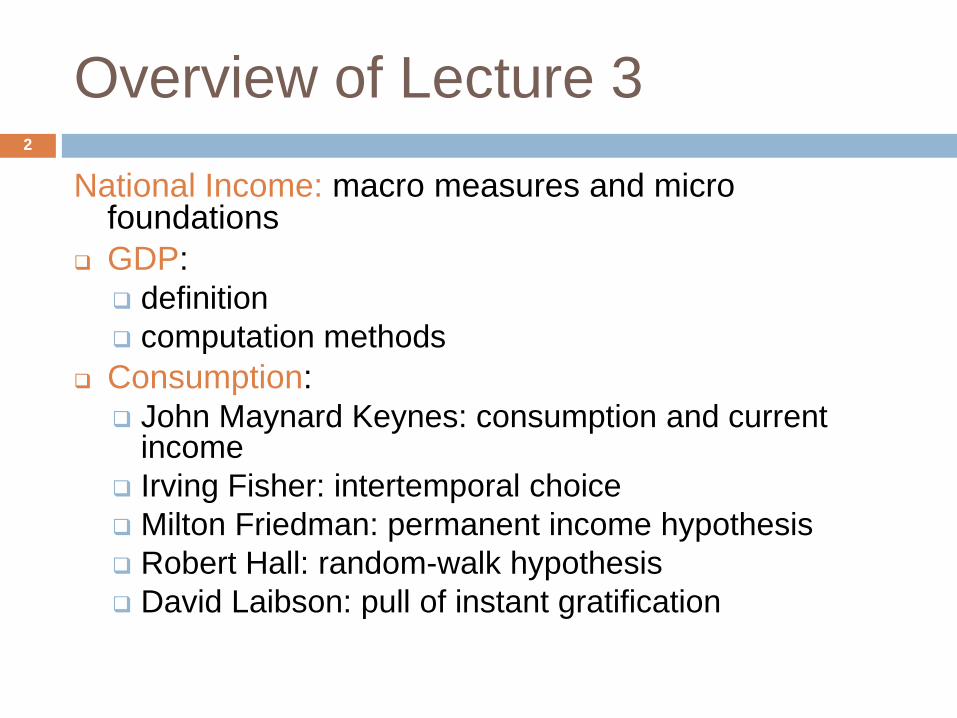
Gross Domestic Product - GDPDefinition

3

GDP = total market value of all final goods and

services within nation’s borders in given time

period

G National P = output produced by nationally-owned

factors of production

ex.: Japanese-owned car production in Kolin

GDP per capita = GDP/ total population

Allows for international comparison

Approximation of difference in living standards

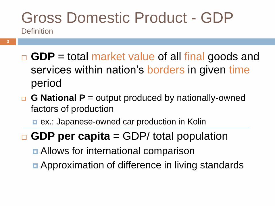
Gross Domestic ProductGlobal overview

4

Source: http://en.wikipedia.org/wiki/File:GDP_PPP_Per_Capita_IMF_2008.png

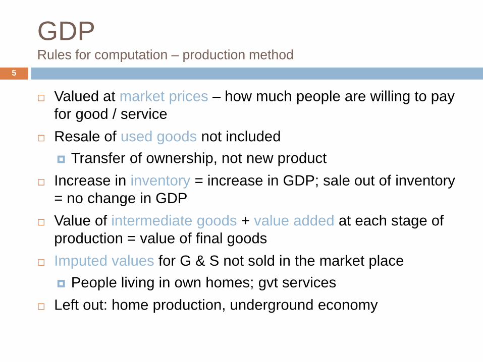
GDPRules for computation – production method

Valued at market prices – how much people are willing to pay

for good / service

Resale of used goods not included

Transfer of ownership, not new product

Increase in inventory = increase in GDP; sale out of inventory

= no change in GDP

Value of intermediate goods + value added at each stage of

production = value of final goods

Imputed values for G & S not sold in the market place

People living in own homes; gvt services

Left out: home production, underground economy

5

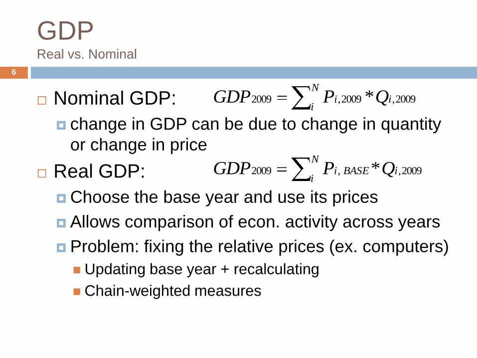
GDPReal vs. Nominal

6

Nominal GDP:

change in GDP can be due to change in quantity

or change in price

Real GDP:

Choose the base year and use its prices

Allows comparison of econ. activity across years

Problem: fixing the relative prices (ex. computers)

Updating base year + recalculating

Chain-weighted measures

2009,2009,2009 * iN

ii QPGDP

2009,,2009 * iN

iBASEi QPGDP

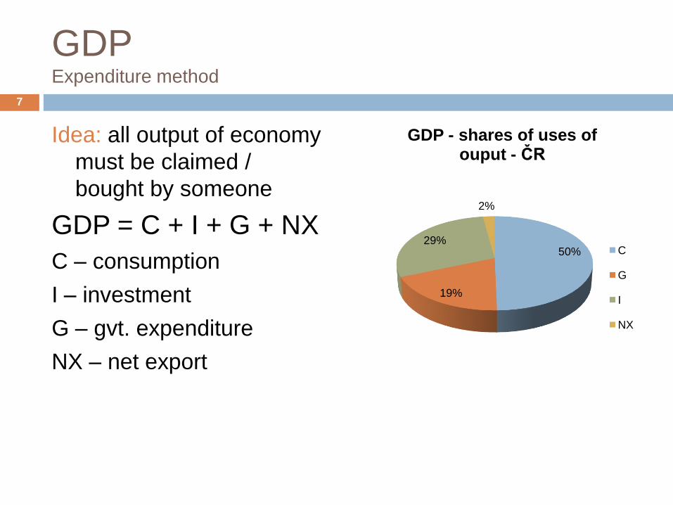
GDPExpenditure method

Idea: all output of economy

must be claimed /

bought by someone

GDP = C + I + G + NX

C – consumption

I – investment

G – gvt. expenditure

NX – net export

7

50%

19%

29%

2%

GDP - shares of uses of ouput - ČR

C

G

I

NX

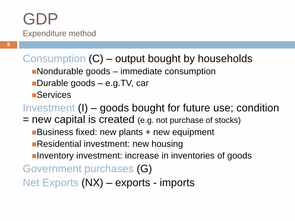
GDPExpenditure method

8

Consumption (C) – output bought by householdsNondurable goods – immediate consumption

Durable goods – e.g.TV, car

Services

Investment (I) – goods bought for future use; condition = new capital is created (e.g. not purchase of stocks)

Business fixed: new plants + new equipment

Residential investment: new housing

Inventory investment: increase in inventories of goods

Government purchases (G)

Net Exports (NX) – exports - imports

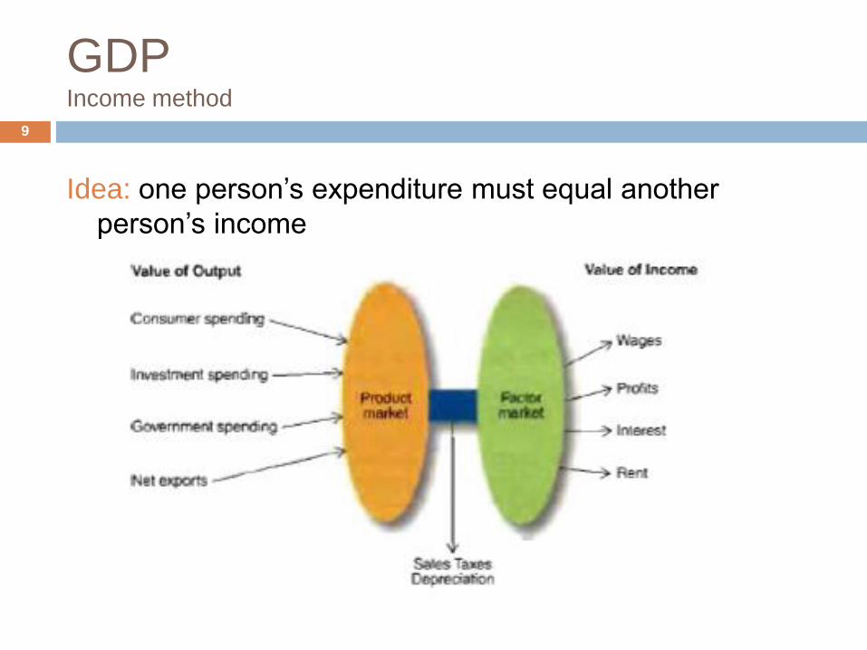
GDPIncome method

Idea: one person’s expenditure must equal another

person’s income

9

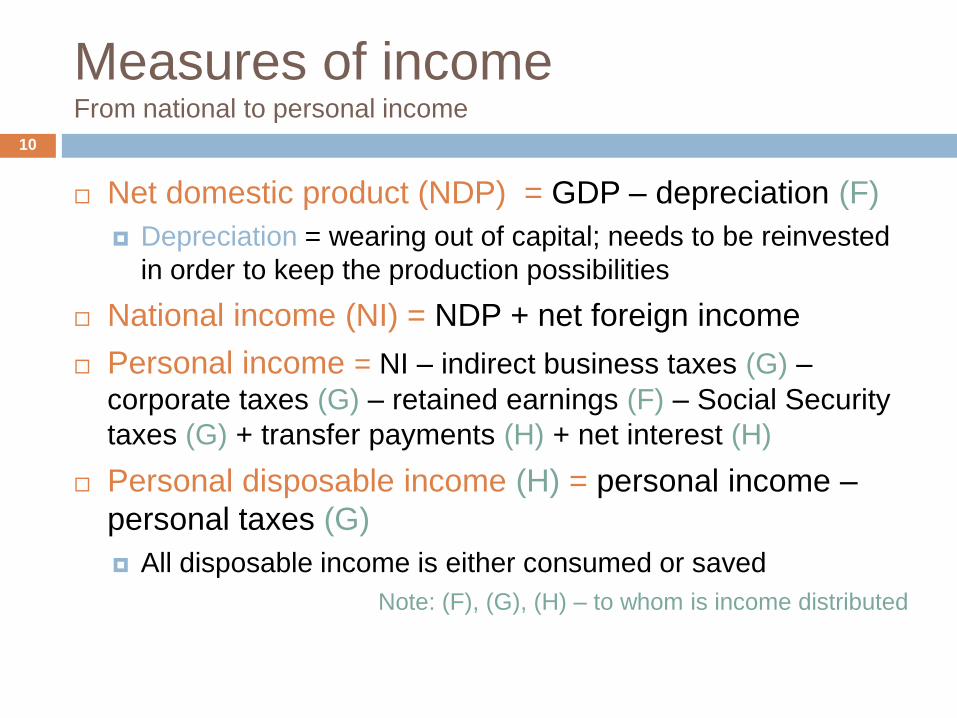
Measures of incomeFrom national to personal income

10

Net domestic product (NDP) = GDP – depreciation (F)

Depreciation = wearing out of capital; needs to be reinvested

in order to keep the production possibilities

National income (NI) = NDP + net foreign income

Personal income = NI – indirect business taxes (G) –

corporate taxes (G) – retained earnings (F) – Social Security

taxes (G) + transfer payments (H) + net interest (H)

Personal disposable income (H) = personal income –

personal taxes (G)

All disposable income is either consumed or saved

Note: (F), (G), (H) – to whom is income distributed

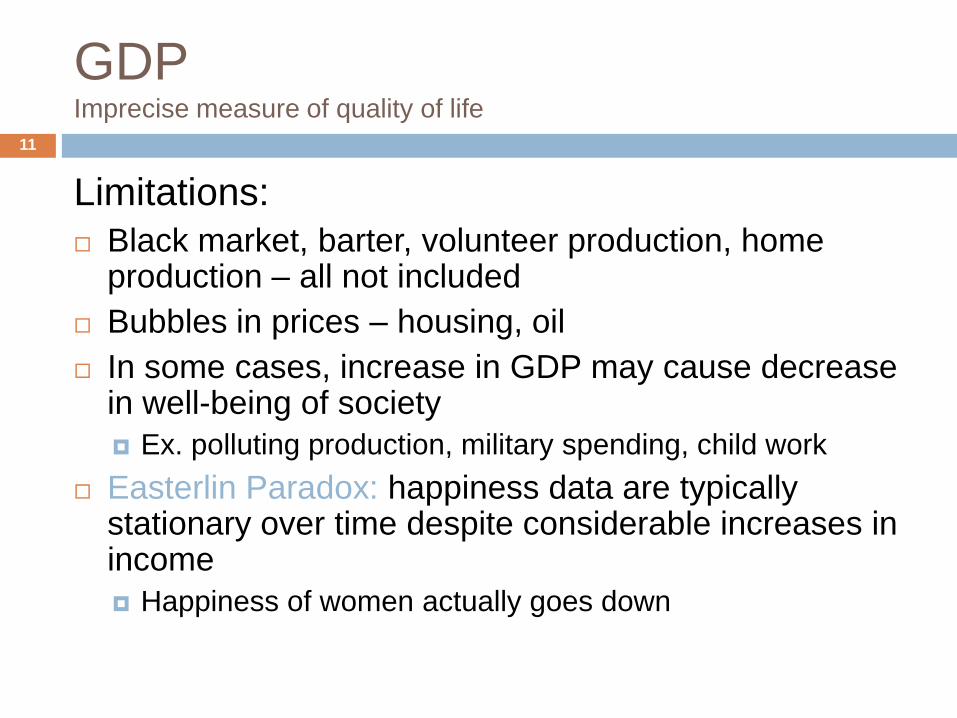
GDPImprecise measure of quality of life

11

Limitations:

Black market, barter, volunteer production, home production – all not included

Bubbles in prices – housing, oil

In some cases, increase in GDP may cause decrease in well-being of society

Ex. polluting production, military spending, child work

Easterlin Paradox: happiness data are typically stationary over time despite considerable increases in income

Happiness of women actually goes down

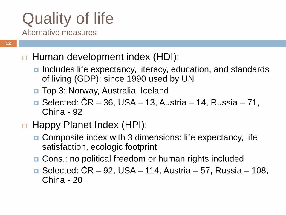
Quality of lifeAlternative measures

12

Human development index (HDI):

Includes life expectancy, literacy, education, and standards of living (GDP); since 1990 used by UN

Top 3: Norway, Australia, Iceland

Selected: ČR – 36, USA – 13, Austria – 14, Russia – 71, China - 92

Happy Planet Index (HPI):

Composite index with 3 dimensions: life expectancy, life satisfaction, ecologic footprint

Cons.: no political freedom or human rights included

Selected: ČR – 92, USA – 114, Austria – 57, Russia – 108, China - 20

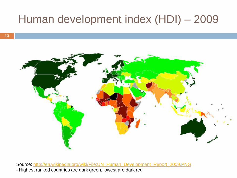
Human development index (HDI) – 2009

13

Source: http://en.wikipedia.org/wiki/File:UN_Human_Development_Report_2009.PNG

- Highest ranked countries are dark green, lowest are dark red

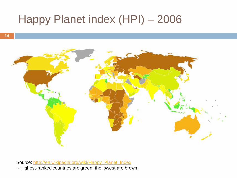
Happy Planet index (HPI) – 2006

14

Source: http://en.wikipedia.org/wiki/Happy_Planet_Index

- Highest-ranked countries are green, the lowest are brown

From Keynes to behavioral theories

ConsumptionMicrofoundations

15

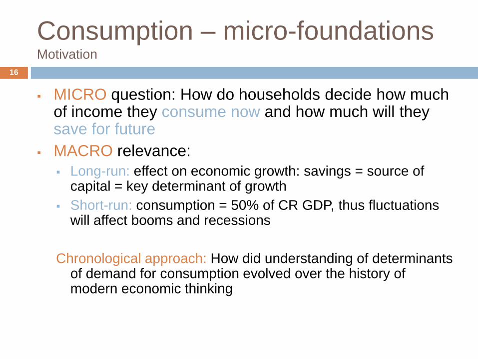
Consumption – micro-foundationsMotivation

16

MICRO question: How do households decide how much of income they consume now and how much will they save for future

MACRO relevance:

Long-run: effect on economic growth: savings = source of capital = key determinant of growth

Short-run: consumption = 50% of CR GDP, thus fluctuations will affect booms and recessions

Chronological approach: How did understanding of determinants of demand for consumption evolved over the history of modern economic thinking

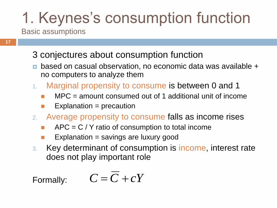
1. Keynes’s consumption functionBasic assumptions

3 conjectures about consumption function

based on casual observation, no economic data was available + no computers to analyze them

1. Marginal propensity to consume is between 0 and 1

MPC = amount consumed out of 1 additional unit of income

Explanation = precaution

2. Average propensity to consume falls as income rises

APC = C / Y ratio of consumption to total income

Explanation = savings are luxury good

3. Key determinant of consumption is income, interest rate does not play important role

Formally:

17

cYCC

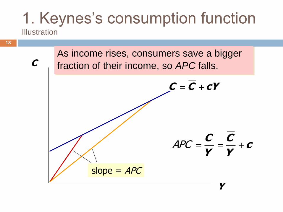
1. Keynes’s consumption functionIllustration

18

C

Y

C C cY

slope = APC

As income rises, consumers save a bigger

fraction of their income, so APC falls.

C Cc

Y YAPC

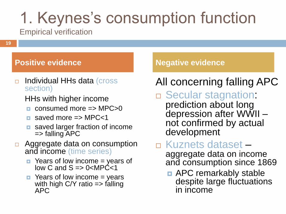
1. Keynes’s consumption functionEmpirical verification

Individual HHs data (cross section)

HHs with higher income

consumed more => MPC>0

saved more => MPC<1

saved larger fraction of income => falling APC

Aggregate data on consumption and income (time series)

Years of low income = years of low C and S => 0<MPC<1

Years of low income = years with high C/Y ratio => falling APC

All concerning falling APC

Secular stagnation: prediction about long depression after WWII –not confirmed by actual development

Kuznets dataset –aggregate data on income and consumption since 1869

APC remarkably stable despite large fluctuations in income

19

Positive evidence Negative evidence

1. Keynes’s consumption functionEmpirical verification - Summary

20

Keynes’s conjectures hold well in cross section

studies of HH’s data and in short time-series,

but fail when long time-series are concerned

MPC between 0 and 1

APC constant with income

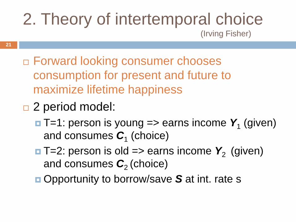
2. Theory of intertemporal choice(Irving Fisher)

21

Forward looking consumer chooses

consumption for present and future to

maximize lifetime happiness

2 period model:

T=1: person is young => earns income Y1 (given)

and consumes C1 (choice)

T=2: person is old => earns income Y2 (given)

and consumes C2 (choice)

Opportunity to borrow/save S at int. rate s

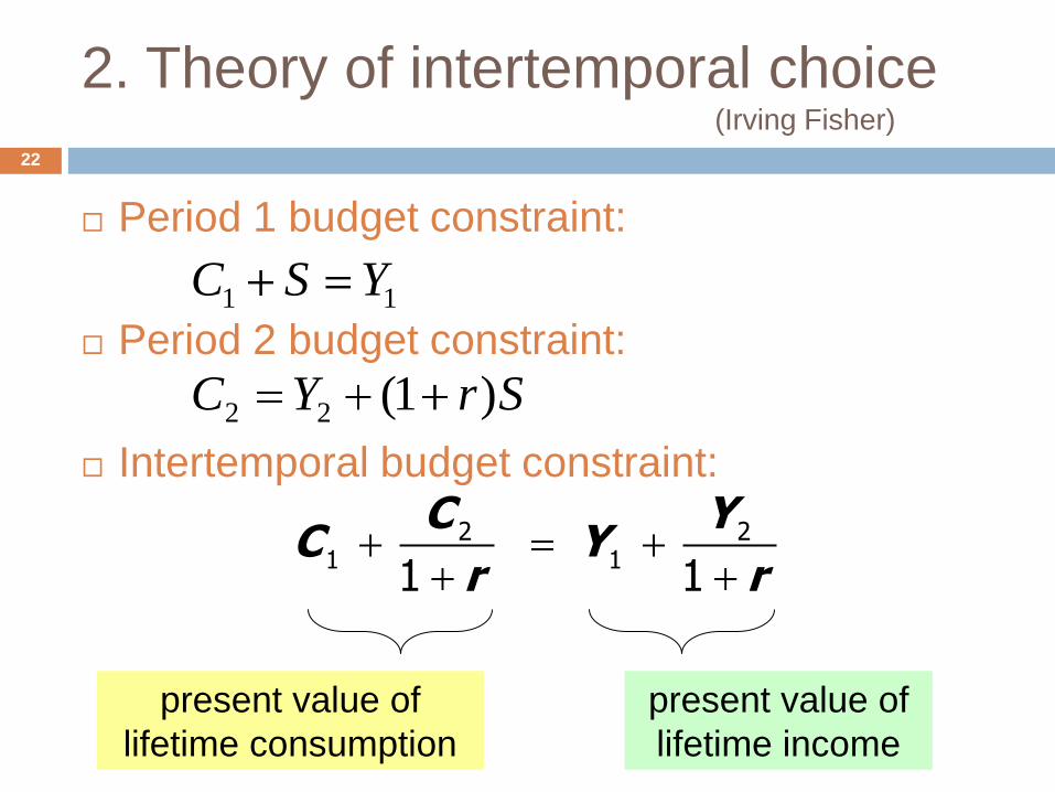
2. Theory of intertemporal choice(Irving Fisher)

22

Period 1 budget constraint:

Period 2 budget constraint:

Intertemporal budget constraint:

2 21 1

1 1

C YC Y

r r

present value of

lifetime consumption

present value of

lifetime income

11 YSC

SrYC )1(22

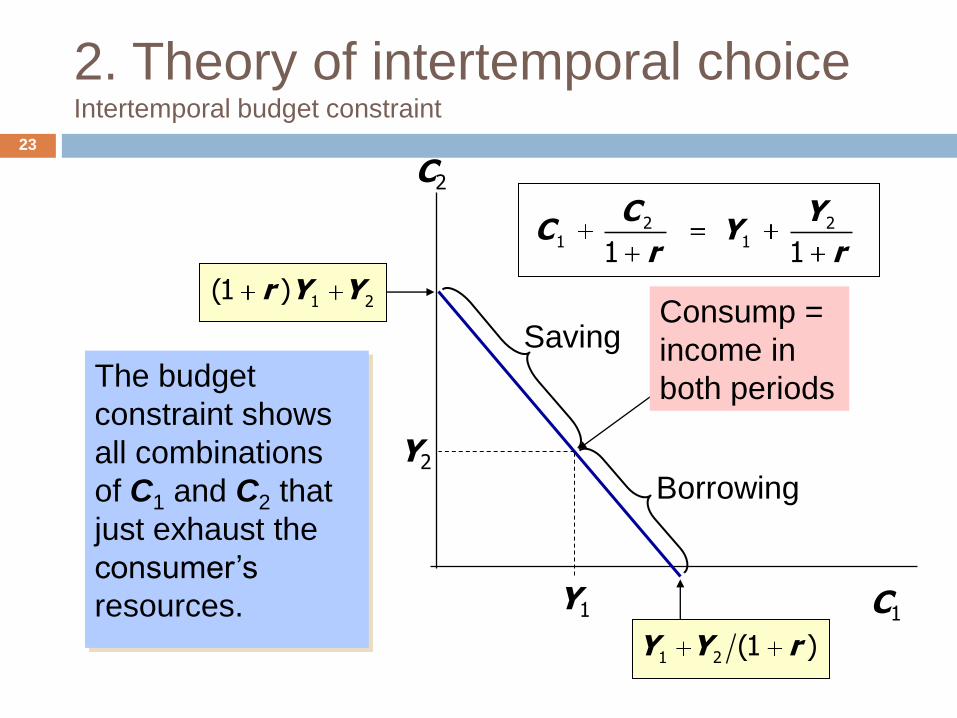
2. Theory of intertemporal choiceIntertemporal budget constraint

23

The budget

constraint shows

all combinations

of C1 and C2 that

just exhaust the

consumer’s

resources. C1

C2

1 2 (1 )Y Y r

1 2(1 )r Y Y

Y1

Y2

Borrowing

SavingConsump =

income in

both periods

2 21 1

1 1

C YC Y

r r

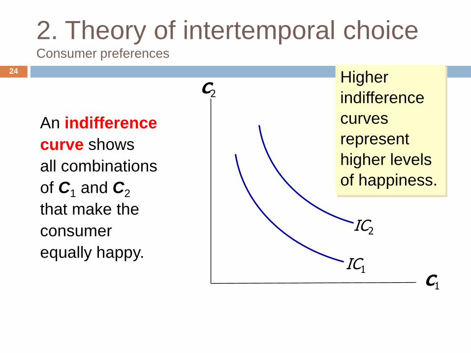
2. Theory of intertemporal choiceConsumer preferences

24

An indifference

curve shows

all combinations

of C1 and C2

that make the

consumer

equally happy.

C1

C2

IC1

IC2

Higher

indifference

curves

represent

higher levels

of happiness.

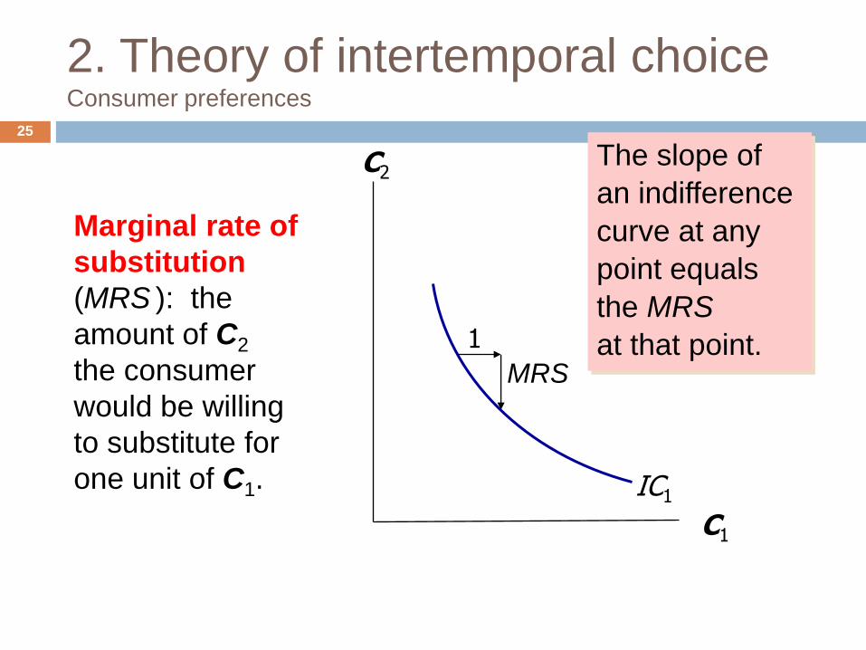
2. Theory of intertemporal choiceConsumer preferences

25

Marginal rate of

substitution

(MRS ): the

amount of C2

the consumer

would be willing

to substitute for

one unit of C1.

C1

C2

IC1

The slope of

an indifference

curve at any

point equals

the MRS

at that point.1

MRS

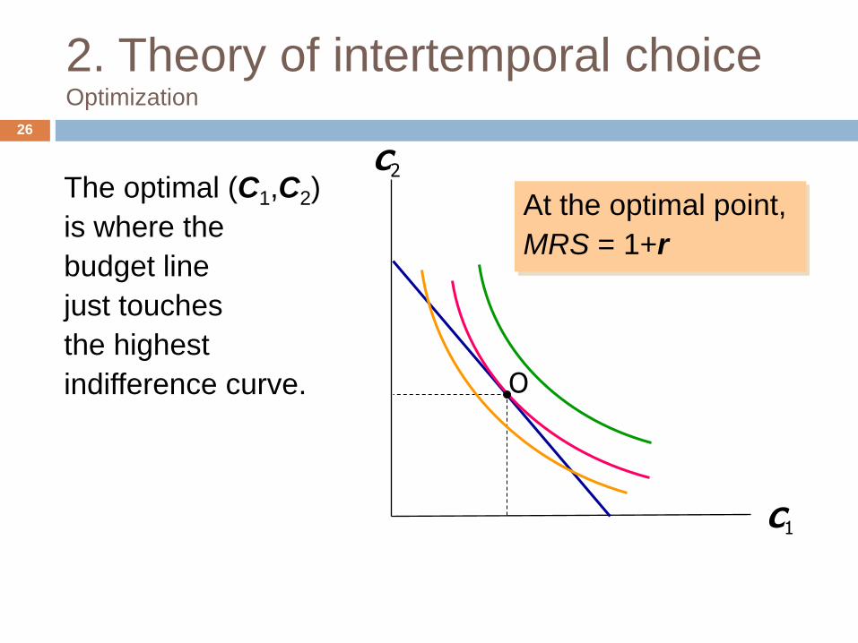
2. Theory of intertemporal choiceOptimization

26

The optimal (C1,C2)

is where the

budget line

just touches

the highest

indifference curve.

C1

C2

O

At the optimal point,

MRS = 1+r

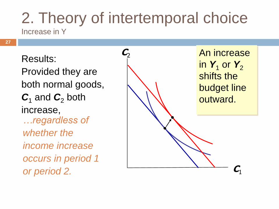
2. Theory of intertemporal choiceIncrease in Y

27

An increase

in Y1 or Y2

shifts the

budget line

outward.

C1

C2Results:

Provided they are

both normal goods,

C1 and C2 both

increase,…regardless of

whether the

income increase

occurs in period 1

or period 2.

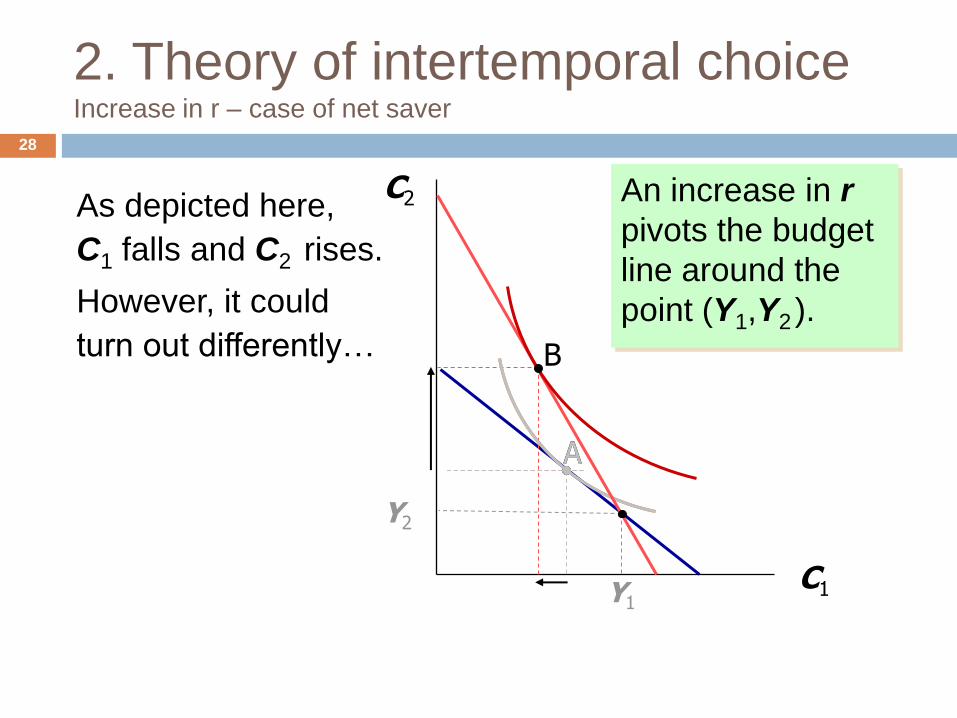
2. Theory of intertemporal choiceIncrease in r – case of net saver

28

A

An increase in r

pivots the budget

line around the

point (Y1,Y2 ).

C1

C2

Y1

Y2

A

B

As depicted here,

C1 falls and C2 rises.

However, it could

turn out differently…

2. Theory of intertemporal choiceIncrease in r – case of net saver

29

income effect: If consumer is a saver, the rise in r makes him better off, which tends to increase consumption in both periods.

substitution effect: The rise in r increases the opportunity cost of current consumption, which tends to reduce C1 and increase C2.

Both effects C2.

Whether C1 rises or falls depends on the relative size of the income & substitution effects

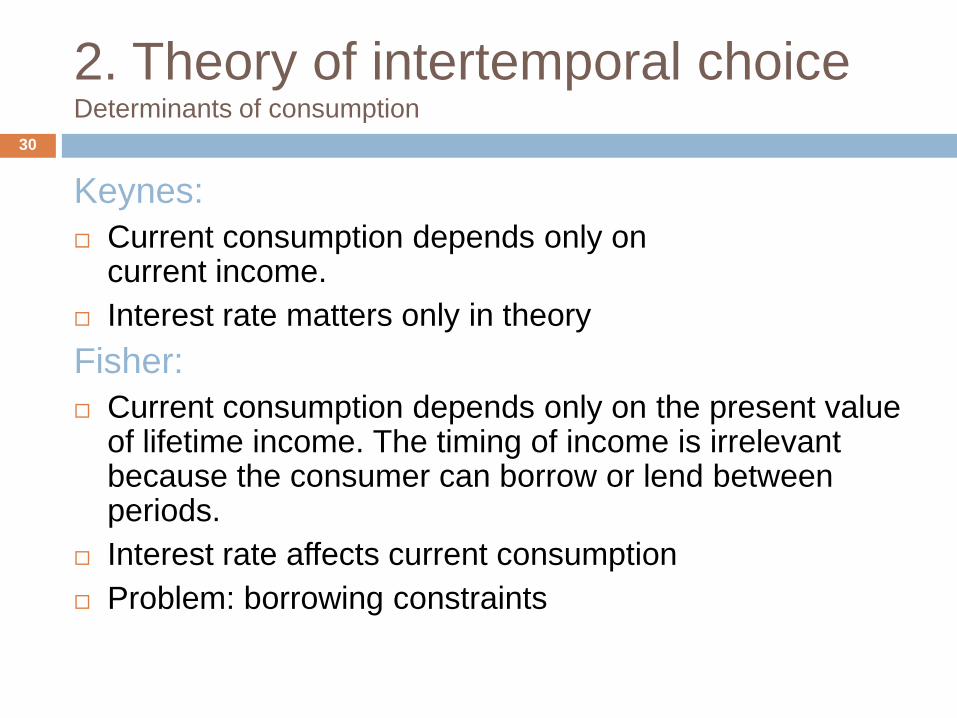
2. Theory of intertemporal choiceDeterminants of consumption

30

Keynes:

Current consumption depends only on current income.

Interest rate matters only in theory

Fisher:

Current consumption depends only on the present value of lifetime income. The timing of income is irrelevant because the consumer can borrow or lend between periods.

Interest rate affects current consumption

Problem: borrowing constraints

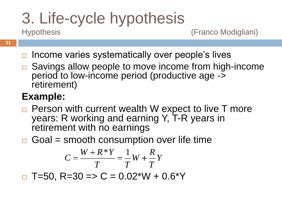
3. Life-cycle hypothesis Hypothesis (Franco Modigliani)

31

Income varies systematically over people’s lives

Savings allow people to move income from high-income period to low-income period (productive age -> retirement)

Example:

Person with current wealth W expect to live T more years: R working and earning Y, T-R years in retirement with no earnings

Goal = smooth consumption over life time

T=50, R=30 => C = 0.02*W + 0.6*Y

YT

RW

TT

YRWC

1*

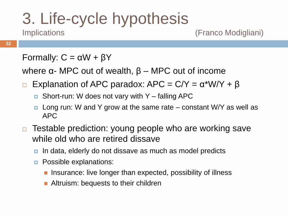
3. Life-cycle hypothesis Implications (Franco Modigliani)

32

Formally: C = αW + βY

where α- MPC out of wealth, β – MPC out of income

Explanation of APC paradox: APC = C/Y = α*W/Y + β

Short-run: W does not vary with Y – falling APC

Long run: W and Y grow at the same rate – constant W/Y as well as

APC

Testable prediction: young people who are working save

while old who are retired dissave

In data, elderly do not dissave as much as model predicts

Possible explanations:

Insurance: live longer than expected, possibility of illness

Altruism: bequests to their children

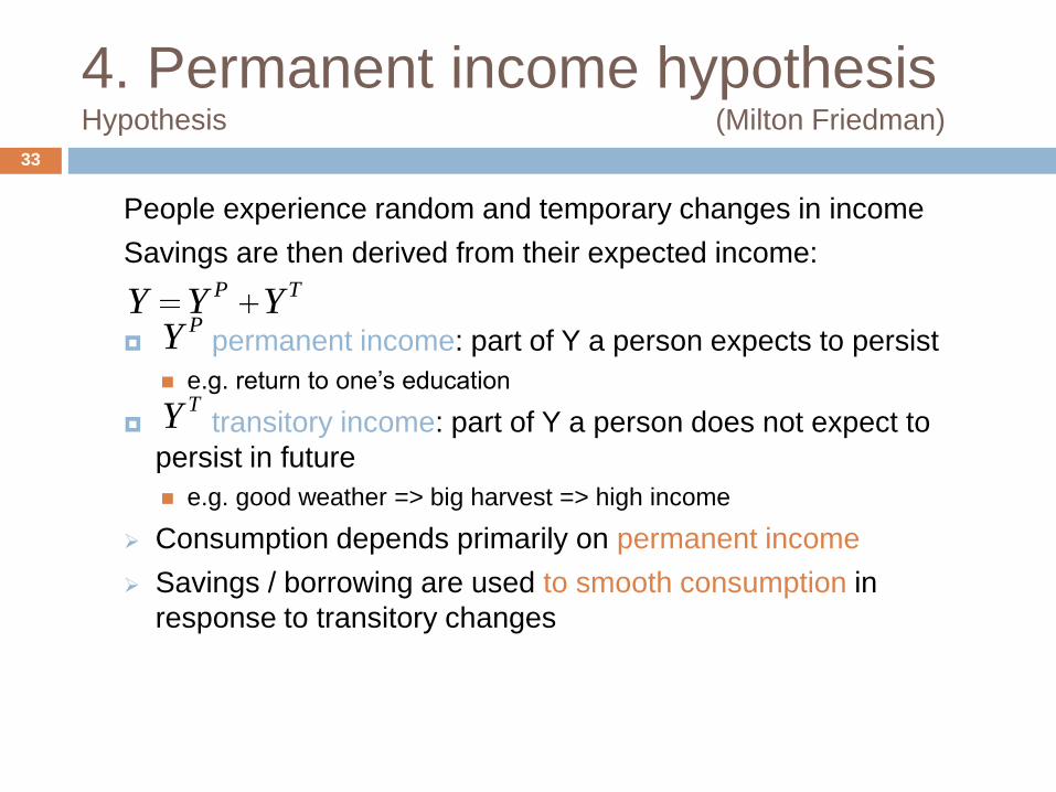
4. Permanent income hypothesis Hypothesis (Milton Friedman)

People experience random and temporary changes in income

Savings are then derived from their expected income:

permanent income: part of Y a person expects to persist

e.g. return to one’s education

transitory income: part of Y a person does not expect to

persist in future

e.g. good weather => big harvest => high income

Consumption depends primarily on permanent income

Savings / borrowing are used to smooth consumption in

response to transitory changes

33

TP YYYPY

TY

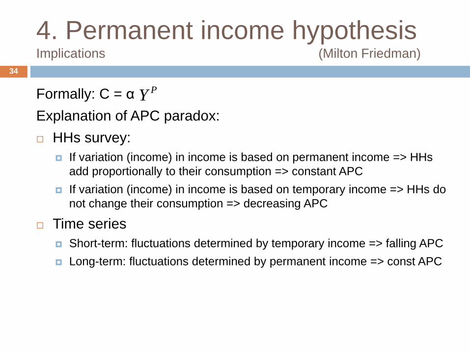
4. Permanent income hypothesis Implications (Milton Friedman)

Formally: C = α

Explanation of APC paradox:

HHs survey:

If variation (income) in income is based on permanent income => HHs

add proportionally to their consumption => constant APC

If variation (income) in income is based on temporary income => HHs do

not change their consumption => decreasing APC

Time series

Short-term: fluctuations determined by temporary income => falling APC

Long-term: fluctuations determined by permanent income => const APC

34

PY

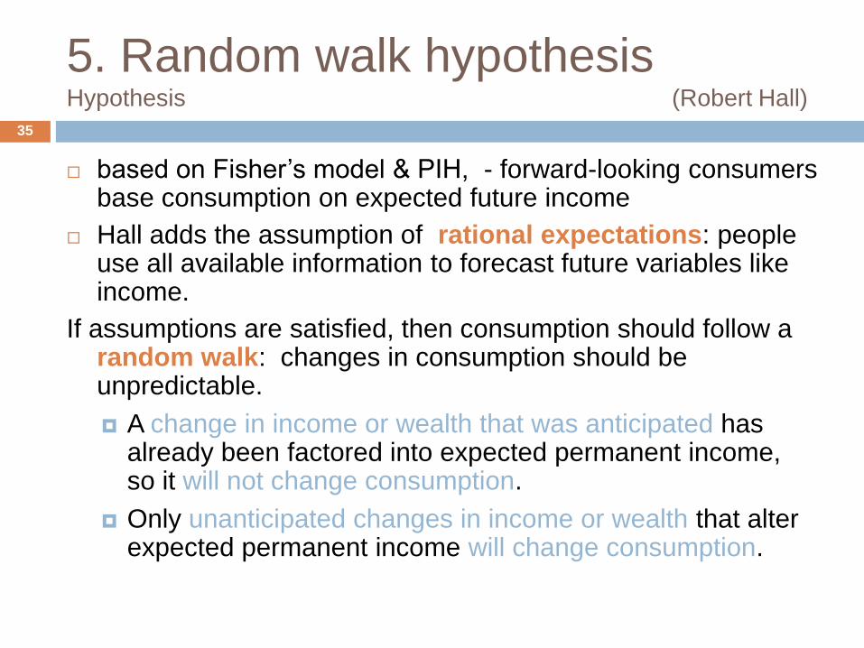
5. Random walk hypothesis Hypothesis (Robert Hall)

35

based on Fisher’s model & PIH, - forward-looking consumers base consumption on expected future income

Hall adds the assumption of rational expectations: people use all available information to forecast future variables like income.

If assumptions are satisfied, then consumption should follow a random walk: changes in consumption should be unpredictable.

A change in income or wealth that was anticipated has already been factored into expected permanent income, so it will not change consumption.

Only unanticipated changes in income or wealth that alter expected permanent income will change consumption.

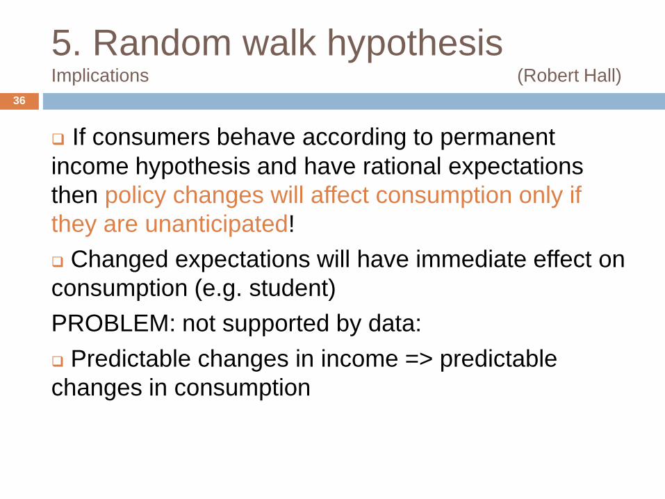
5. Random walk hypothesis Implications (Robert Hall)

36

If consumers behave according to permanent

income hypothesis and have rational expectations

then policy changes will affect consumption only if

they are unanticipated!

Changed expectations will have immediate effect on

consumption (e.g. student)

PROBLEM: not supported by data:

Predictable changes in income => predictable

changes in consumption

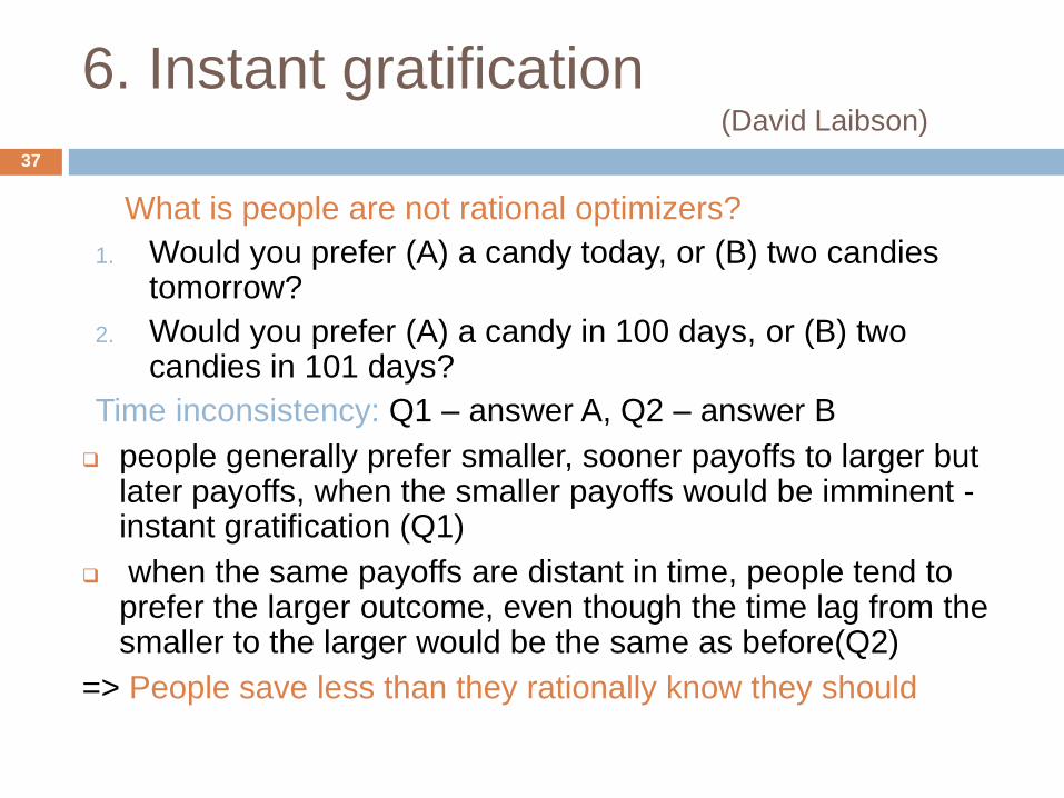
6. Instant gratification(David Laibson)

What is people are not rational optimizers?

1. Would you prefer (A) a candy today, or (B) two candies tomorrow?

2. Would you prefer (A) a candy in 100 days, or (B) two candies in 101 days?

Time inconsistency: Q1 – answer A, Q2 – answer B

people generally prefer smaller, sooner payoffs to larger but later payoffs, when the smaller payoffs would be imminent -instant gratification (Q1)

when the same payoffs are distant in time, people tend to prefer the larger outcome, even though the time lag from the smaller to the larger would be the same as before(Q2)

=> People save less than they rationally know they should

37

Summary

Keynes: consumption depends primarily on current

income

Recent work: consumption also depends on

Expected future income

Wealth

Interest rates

Borrowing constraints

Psychological factors

38