Optimal Government Policies in Models withHeterogeneous Agents∗

Radim BohacekCERGE-EI

Michal KejakCERGE-EI

Abstract

In this paper we develop a new methodology for finding optimalgovernment policies in economies with heterogeneous agents. Themethodology is solely based on three classes of equilibrium conditionsfrom the government’s and individual agent’s optimization problems:1) the first order conditions; 2) the stationarity condition on the dis-tribution function; and, 3) the aggregate market clearing conditions.These conditions form a system of functional equations which we solvenumerically. The solution takes into account simultaneously the effectof government policy on individual allocations and (from the govern-ment’s point of view) optimal distribution of agents in the steadystate. This general methodology is applicable to a wide range of op-timal government policies in models with heterogeneous agents. Weillustrate it on a steady state Ramsey problem with heterogeneousagents, finding the optimal tax schedule.

JEL Keywords: Optimal macroeconomic policy, optimal taxation,computational techniques, heterogeneous agents, distribution ofwealth and income

∗Contact: CERGE-EI, Politickych veznu 7, 111 21 Prague 1, Czech Republic. Email:radim.bohacek@cerge-ei.cz, michal.kejak@cerge-ei.cz. First version: September 2002. Forhelpful comments we thank Jim Costain, Max Gillman, Marek Kapicka, Josep Pijoan-Mas, Galyna Vereshchagina, and the participants at the CNB/CERGE-EI Macro Work-shop 2004, SED 2004 conference, ESEM 2006 in Vienna, the Macroeconomic Seminar atthe Federal Reserve Bank of Minneapolis, University of Southern California and CardiffUniversity Business School. We are especially grateful to Michele Boldrin and Tim Ke-hoe for their support and advice. Anton Tyutin and Jozef Zubricky provided excellentresearch assistance. All errors are our own. CERGE-EI is a joint workplace of the Centerfor Economic Research and Graduate Education, Charles University, and the EconomicsInstitute of the Academy of Sciences of the Czech Republic.

1

Abstrakt

V teto praci navrhujeme novou metodologii pro hledanı optimalnıch vladnıchpolitik v ekonomikach s heterogennımi agenty. Tato metodologie je zalozenavylucne na trech trıdach rovnovaznych podmınek zıskanych z optimalizacnıchproblemu pro vladu a pro individualnı agenty: 1) podmınky prvnıho radu; 2)podmınka stacionarity pro distribucnı funkci; a 3) agregatnı podmınky pro trznırovnovahu. Tyto podmınky tvorı system funkcionalnıch rovnic, jejichz resenı jezıskano pomocı numerickych metod. Zıskane resenı bere soucasne do uvahy ucinekvladnıch politik jak na individualnı alokace tak na (z pohledu vlady) optimalnıdistribuci agentu v ustalenem stavu. Tato obecna metodologie je pouzitelna nasiroky okruh optimalnıch vladnıch politik v modelech s heterogennımi agenty. Myji demonstrujeme na Ramsey problemu v ustalenem stavu s heterogennımi agenty,tzn.na hledanı optimalnı danove funkce.

JEL Classification: C61, C68, D30, D58

2

1 Introduction

This paper provides a new methodology for computing equilibria which allows the sta-

tionary distribution of wealth and income to be a part—perhaps the most important—

of a government optimization problem. This general solution method is applicable to

a wide range of optimal government policies in models with heterogeneous agents. We

formulate the optimal government policy problem as an “operator” problem subject to a

system of constraints: 1) the first order conditions from the individual agent’s problem;

2) the stationarity condition on the distribution function; and, 3) the aggregate market

clearing conditions. The first order conditions of the government operator problem form

a system of functional equations in individual agents’ and the government’s policies and

in the distribution function over agents’ individual state variables. We solve this system

numerically by the projection method.

It should be emphasized that our approach does not use any additional restrictions on

or assumptions of the equilibrium allocations but is strictly derived from the first order

and envelope conditions and from the stationarity of the endogenous distribution in the

steady state. Our main contribution is in the formulation of the functional equations

for the government problem and for the stationary distribution over individual state

variables. In this way, we are able to solve simultaneously for the optimal government

policy, for the optimal individual allocations, and (from the government’s point of view)

for the optimal distribution of agents in the steady state. To our knowledge, this paper

is the first one that provides a solution method for this kind of problem.

We illustrate this general methodology on a steady state Ramsey problem with

heterogeneous agents. We recast the original Ramsey (1927) and Lucas (1990) normative

question for an economy with heterogeneous agents: What choice of a tax schedule will

lead to maximal social welfare in the steady state, consistent with given government

consumption and with market determination of quantities and prices? What is the

welfare differential with respect to social welfare resulting from the existing progressive

3

tax schedule in the U.S. economy and as well as from the usual flat-tax reform?

The tradeoff between efficiency and income distribution plays a central role in ana-

lyzing tax policy. In dynamic, general equilibrium models with household heterogeneity

from uninsurable idiosyncratic risk, the optimal tax schedule balances the gains from

offering insurance against the efficiency losses from distorting taxes. In our example, we

find a welfare maximizing tax schedule on total income from labor and capital which

takes into account simultaneously its effects on agents’ allocations and on the station-

ary distribution of agents in a steady state. Previous models analyzing the effects of

government policies in this class of models were limited to a sub-optimal policy reform

exogenously imposed on the model. Within the context of optimal taxation, several pa-

pers have analyzed the steady state implications (and transition paths) resulting from

an ad hoc flat-tax reform or from an ad hoc removal of double taxation of capital income.

In this paper, we solve for the optimal steady state tax schedule chosen by a govern-

ment maximizing the average welfare. In order to evaluate the benefits of the optimal

tax schedule, we compare the steady state aggregate levels, welfare, efficiency and dis-

tribution of resources associated with the optimal tax schedule to a simulated steady

state of the U.S. economy with the existing progressive tax schedule and to a steady

state resulting from a standard flat-tax reform.

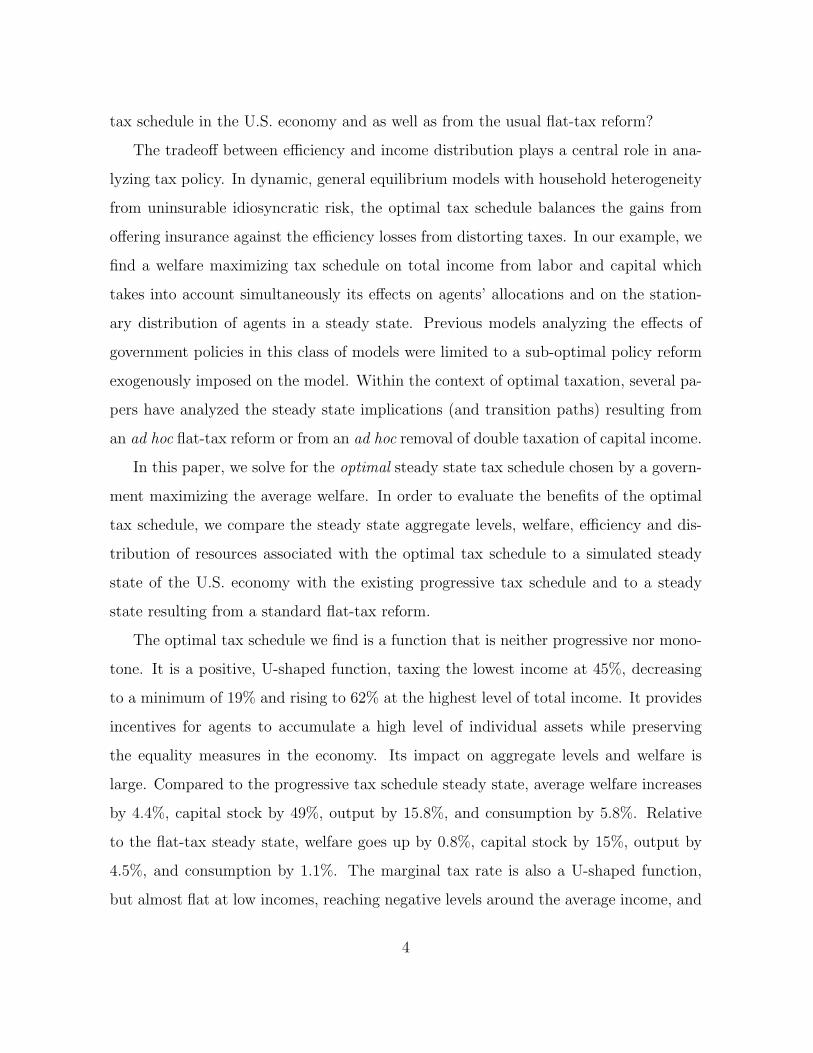
The optimal tax schedule we find is a function that is neither progressive nor mono-

tone. It is a positive, U-shaped function, taxing the lowest income at 45%, decreasing

to a minimum of 19% and rising to 62% at the highest level of total income. It provides

incentives for agents to accumulate a high level of individual assets while preserving

the equality measures in the economy. Its impact on aggregate levels and welfare is

large. Compared to the progressive tax schedule steady state, average welfare increases

by 4.4%, capital stock by 49%, output by 15.8%, and consumption by 5.8%. Relative

to the flat-tax steady state, welfare goes up by 0.8%, capital stock by 15%, output by

4.5%, and consumption by 1.1%. The marginal tax rate is also a U-shaped function,

but almost flat at low incomes, reaching negative levels around the average income, and

4

then rising to positive levels.

The efficiency and distributional effects of the optimal tax are the main mechanisms

behind these large changes. Related to the former are the general equilibrium effects: a

higher stock of capital increases productivity of labor and, therefore, the income of poor

agents. For the latter, the optimal tax schedule concentrates agents around the mean at

high levels of wealth, something that a social planner with access to lump-sum transfers

would do. The high tax rate at low income levels provides incentives for these agents

to save more. The even higher tax rate on high income discourages further savings by

the wealthiest agents. In the middle of the total income levels, the tax rate is lower

than the one found for the flat-tax reform. In this way, the optimal tax schedule solves

the tradeoff between efficiency and equality by altering individual real incomes. For

comparison, the flat tax also increases aggregate levels but does not take into account

the distribution of agents. On the other hand, the progressive tax schedule provides too

much short-run insurance at the cost of long-run average levels.

Finally, in order to evaluate the short run costs of the optimal tax reform, we compute

transitions from the progressive and the flat-rate tax schedule steady states to the steady

state of the optimal tax schedule. One of our main results is that a majority of the

population, 73%, would benefit from a reform that replaces the progressive tax schedule

with the optimal tax schedule. On the other hand, only one third of agents would support

the reform in the flat rate steady state. These results as well as a detailed efficiency and

distributional analysis is described in great detail in the following sections.

We limit our example to the optimal tax schedule on total income from labor and

capital that is needed to raise a given fraction of GDP. There are several reasons why we

choose this setup. First, the tax on total income enables us to study a distortionary tax

system with a non-degenerate distribution of agents in a steady state. If the government

had access to lump-sum, first best taxation, the model would collapse to a representative

agent one. Second, to a large extent the current U.S. tax code does not distinguish

between sources of taxable income. The last reason for a simple tax on the total income

5

is the complexity of the problem we solve.

By focusing on a steady state analysis and by imposing a single tax rate on labor

and capital income, we are for now avoiding two important issues related to optimal

taxation: the issue of time-consistency and the issue of the optimal capital income

tax rate in the steady state. With respect to the former, our government is fully and

credibly committed, and the tax schedule is constant over time.1 The latter issue is to

some extent mitigated by the findings of Aiyagari (1995), who showed that for our class

of models with incomplete insurance markets and borrowing constraints, the optimal

tax rate on capital income is positive even in the long run.2

Our approach is different from the current contributions to the optimal taxation

literature. Based on the original work of Mirrlees (1971) and Mirrlees (1976), Kocher-

lakota (2003), Golosov, Kocherlakota, and Tsyvinski (2003) and ?) study optimal social

planner policies with asymmetric information. In such an environment, positive capital

income taxes are optimal despite the associated efficiency loss, and informational fric-

tions are necessary for a characterization of the optimal policies. Compared to these

papers, we solve for the optimal tax schedule within the standard neoclassical, general

equilibrium, full information and full commitment economy with heterogeneous agents

and incomplete markets. Moreover, we characterize the set of admissible tax functions

that satisfy the definition of stationary recursive competitive equilibria and are consis-

tent with each agent’s maximization problem.

The closest paper to ours is Conesa and Krueger (2004), who compute the optimal

progressivity of the income tax code in an overlapping generations economy. They search

in a class of monotone tax functions to find a welfare maximizing tax schedule. We

show in this paper that, first, limiting the analysis to monotone functions seems rather

1For the time-consistency problem, see Kydland and Prescott (1977) and a recent contribution by

Klein and Rios-Rull (2004).2The optimal capital tax in an economy with two types of agents is discussed in Chamley (1986)

and Judd (1985).

6

restrictive with respect to welfare maximization. Second, our computational method

based on the government optimality conditions improves the welfare criterion by several

percentage points compared to the one found by simple search methods.

We are aware of the other issues that are important for the analysis of optimal taxa-

tion. We do not consider technology or population growth; we do not model a life-cycle

earnings process like Ventura (1999). The tax revenues are not given back to the agents;

we abstract from public goods. We study the simplest utility maximization problem

on the consumption-investment margin. However, we would like to stress here that

our methodology can be applied to any optimal government policy problem, including

that with endogenous labor supply or separate taxation of labor and capital incomes.

Finally, in future research we also plan to analyze a much more difficult problem, that

of a stationary competitive equilibrium which is the limit of the optimal dynamic tax

schedule (again, simple search methods cannot be used for this task).

The paper is organized as follows. The following section describes the economy

with heterogeneous agents, defines the stationary recursive competitive equilibrium and

the Ramsey problem. Section 3 formulates the equilibrium as a system of functional

equations and defines the operator Ramsey problem. Section 4 characterizes the optimal

tax schedule by the first order necessary conditions for the operator Ramsey problem.

The computational projection method is described in Section 5. Section 6 presents

the results and Section 7 concludes. The Appendix contains the proof of the main

proposition.

2 The Steady State Ramsey Problem

This Section describes the economy, defines the stationary recursive competitive equi-

librium and formulates the Steady State Ramsey Problem. The economy is populated

by a continuum of infinitely lived agents on a unit interval. Each agent has preferences

7

over consumption given by the utility function

E

[ ∞∑t=0

βtu(ct)

],

where β ∈ (0, 1) and u : R+ → R is twice continuously differentiable, strictly increasing

and a strictly concave function. We assume that the utility function satisfies the Inada

conditions.

In each period, each agent receives an idiosyncratic labor productivity shock which

takes on values in a finite set of real numbers, z ∈ Z = {z1, z2, . . . , zJ}. The shock

is measured in efficiency units and follows a first-order Markov chain with a transition

function Q(z, z′) = Prob(zt+1 = z′|zt = z). We assume that Q is monotone, satisfies the

Feller property and the mixing condition defined in Stokey, Lucas, and Prescott (1989).

As the labor productivity shock is independent across agents, there is no uncertainty at

the aggregate level.

All agents are initially endowed with a nonnegative stock of capital. In each period,

each agent supplies his realized labor endowment and accumulated capital stock k to

competitive firms operating constant returns to scale production technology. We restrict

the accumulated capital to be nonnegative, k ∈ B = [kL,∞), where kL = 0. The capital

stock depreciates at the rate δ ∈ (0, 1).

Finally, there is a government that finances its expenditures by taxing the agents

in the economy. We assume that the government expenditures are a fixed percentage

of total output, they are not returned to the agents and the government cannot use

the first best, lump-sum taxation. We assume that the government has access only to

proportional taxation of total income from labor and capital.3

The ultimate goal is to analyze the economy as a steady-state Ramsey problem with

heterogeneous agents. In particular, we seek an optimal, time invariant tax schedule

in a stationary recursive competitive equilibrium that will lead to maximal average

3We want to emphasize here that our methodology is equally applicable to the case in which gov-

ernment consumption is a given number.

8

utility in the steady state, consistent with given government consumption and with

market determination of quantities and prices. Throughout the whole paper, the value

function, the policy functions, the distribution function, aggregate levels and prices all

depend on the tax schedule.

In the competitive equilibrium, given any time-invariant tax schedule τ , agents accu-

mulate aggregate capital stock K used by a representative firm together with inelastically

supplied aggregate effective labor L in the production technology F (K,L) = AKαL1−α,

with technology parameters A > 0 and α ∈ (0, 1). Profit maximization implies the

following factor prices:

r = FK(K,L)− δ and w = FL(K, L). (1)

In each period, an agent inelastically supplies his labor endowment at wage w, rents

capital stock at interest rate r, and maximizes his or her utility by choosing consumption

and a level of capital stock for the next period. We preserve heterogeneity in the economy

by closing insurance markets so that the agents can only imperfectly insure against

idiosyncratic labor productivity shocks by precautionary savings.

Given competitive factor prices (r, w), the government finances its expenditures by

a proportional tax on each agent’s total income y from labor and capital,

y(k, z) = rk + wz.

Then, the tax schedule on total income is the function

τ : R+ → R,

so that an agent with total income y faces tax rate τ(y) and receives after tax income

(1− τ(y))y.

We will model the economy in a stationary recursive competitive equilibrium. For

time-invariant tax schedule τ , such an equilibrium exhibits constant factor prices, con-

stant levels of aggregate variables, and a stationary distribution of agents over their

9

individual states. An agent’s individual state is the pair (k, z) ∈ B × Z denoting his or

her accumulated stock of capital and the realized labor productivity shock, respectively.

Taking the factor prices (r, w) and the tax schedule τ as given, an agent (k, z) solves

the following dynamic programming problem

v(k, z) = maxc,k′

{u(c) + β

∑

z′v(k′, z′) Q(z, z′)

}, (2)

subject to budget constraint

c + k′ ≤ (1− τ(y))y + k, (3)

and no borrowing constraint

k′ ≥ 0, (4)

where taxable income is defined as

y = rk + wz.

For time-invariant tax schedule τ , probability measure λ defined on subsets of the

state space describes the heterogeneity of the agents over their individual state (k, z).

Let (B,B) and (Z,Z) be measurable spaces, where B denotes the Borel sets that are

subsets of B, and Z is the set of all subsets of Z. Let (B×Z,B×Z, λ) be a probability

space. We interpret λ as a probability measure describing the fractions of agents with

the same individual state.

The policy function for next-period capital k′(k, z) and the Markov process for the

productivity shock generate a law of motion:

λ′(B′, z′) =∑

z

∫

{(k,z)∈B×Z: k′(k,z)∈B′}Q(z, z′) λ(k, z) dk, (5)

for all (B′, z′) ∈ B×Z. According to this law of motion, the fraction of agents that will

begin the next period with capital stock in set B′ and productivity shock z′ is given by

all those agents that transit from their current shock z to shock z′ and whose optimal

decision for capital accumulation belongs to B′.

10

The government budget constraint is, for government expenditures G, expressed as

the fixed fraction g of the total output Y ,

g ≤ G

Y=

∑z

∫τ(y(k, z))y(k, z) λ(k, z) dk

F (K,L). (6)

Definition 1 (Stationary Recursive Competitive Equilibrium) Given a time-

invariant tax schedule τ , a stationary recursive competitive equilibrium is the value

function v, policy functions (c, k′), probability measure λ, and prices (r, w), such that

1. given prices and the tax schedule, the policy functions solve each agent’s optimiza-

tion problem (2)-(4);

2. firms maximize profit (1);

3. the probability measure (5) is time invariant;

4. the government budget constraint (6) holds at equality;

5. the capital and labor markets clear,

K =∑

z

∫k′(k, z) λ(k, z) dk; (7)

L =∑

z

∫z λ(k, z) dk, (8)

6. and the allocations are feasible,

∑z

∫[c(k, z) + k′(k, z)] λ(k, z) dk + G = F (K, L) + (1− δ)K. (9)

Note that the aggregate feasibility constraint is implied from the other market clear-

ing conditions by Walras’ law. Since labor supply is inelastic, the labor market clears

by construction.

11

2.1 The Existence of Stationary Recursive Competitive Equi-

librium

Given tax schedule τ and prices, each agent’s optimal policy function k′(k, z) for all

(k, z) ∈ B × Z can be derived from the first order condition

u′(c) ≥ β∑

z′u′(c′) [(1− τ(y′)− τ ′(y′)y′) r + 1] Q(z, z′),

where c′ = (1−τ(y′)) y′+k′−k′′ and y′ = rk′+wz′. Because we study a stationary recur-

sive competitive equilibrium, the two period ahead saving function k′′ = k′(k′(k, z), z′).

Note that the agent also takes into account the effect of his current savings decisions on

tomorrow’s marginal tax, τ ′(y′).

Because the tax schedule is an arbitrary function, we must ensure that the first order

approach is valid. In order to characterize the admissible tax functions and to prove

the Schauder Theorem for economies with distortions, we follow the notation in Stokey,

Lucas, and Prescott (1989), Chapter 18. For each agent (k, z) ∈ B × Z with taxable

income y(k, z) = rk + wz, denote the after-tax gross income as

ψ(k, z) ≡ (1− τ(y(k, z))) y(k, z) + k.

Using ψ(k, z), rewrite the Euler equation4 as

u′(ψ(k, z)− k′(k, z)) = β∑

z′u′(ψ(k′(k, z), z′)− k′(k′(k, z), z′))ψ1(k

′(k, z), z′)Q(z, z′),

where

ψ1(k′(k, z), z′) = (1− τ(y(k′(k, z), z′))− τ ′(y(k′(k, z), z′)) y(k′(k, z), z′)) r + 1

is the marginal after-tax return on an extra unit of investment. In the following theorem

we establish the validity of the first order approach and the existence of the competitive

equilibrium.

4Here, we describe only the interior solution. We analyze the case of borrowing constrained agents

in the following Sections.

12

Theorem 1 If for each (k, z) ∈ B × Z, given a tax schedule τ : R+ → R,

1. ψ1(k, z) > 0, and

2. ψ is quasi-concave,

then the solution to each agent’s maximization problem and the stationary recursive

competitive equilibrium exist.

The proof of Theorem 1 is in the Appendix.

The following corollary characterizes the set of admissible tax schedules that satisfy

the conditions of Theorem 1. For this purpose, define k as the maximal sustainable

capital for any agent (for a detailed definition see the proof of Theorem 1). Let w

and r denote some exogenously imposed, non-binding lower and upper bounds for the

equilibrium wage and interest rate, respectively, and let z and z stand for the lowest

and highest productivity shocks. Finally, ετy(y) ≡ τ ′(y)

τ(y)y is the elasticity of the tax rate

to the taxable income.

Corollary 1 (Admissible Tax Schedule Functions) Let C2(R+) be a set of con-

tinuously differentiable functions from R+ to R. If tax schedule function τ ∈ C2(R+)

belongs to the set of admissible tax schedules Υ,

Υ =

{τ ∈ C2(R+) : τ(y)

(1 + ετ

y

)< 1 +

1

r

}

for all y ∈ [wz, rk + wz], then it satisfies the conditions of Theorem 1.

The above statement follows directly from the fact that ψ1(k, z) > 0 and that ψ is quasi-

concave. The corollary implies that there exists an upper bound on the marginal tax

rate, τ(y)(1 + ετ

y

). This upper bound is not likely to bind for a very wide range of tax

schedules.5 We want to stress here that while numerically solving for the optimum tax

5For a realistic equilibrium interest rate r = 0.05, the upper bound is equal to 21. Therefore, at a

high tax rate level, say 42%, the elasticity of the tax schedule would have to be equal to an extreme

level 49 in order to violate the admissibility condition.

13

schedule we do not impose any of these exogenous bounds but we check the admissibility

of the optimal tax schedule ex post.

The goal of our paper is to solve for the following Steady State Ramsey Problem.

Definition 2 (Steady State Ramsey Problem) A solution to the Ramsey problem

for a stationary economy with heterogeneous agents is an admissible time-invariant tax

schedule τ ∈ Υ that maximizes social welfare in the steady state

maxτ

∑z

∫v(k, z) λ(k, z) dk,

consistent with a given government consumption and with allocations satisfying the def-

inition of the stationary recursive competitive equilibrium, where v : B × Z → R is the

value function of individual agents and λ : B×Z → [0, 1] is the stationary distribution.

It is easy to show that the above specification of the Steady State Ramsey Problem is

equivalent to maximizing the average current period utility,

maxτ

∑z

∫u(c(k, z)) λ(k, z) dk.

In the following Sections, we will characterize the optimal tax schedule using this latter

specification.

3 The Operator Steady State Ramsey Problem

In this Section we study the Steady State Ramsey Problem of choosing the tax schedule

to maximize utilitarian social welfare subject to the constraints that the government’s

budget is balanced and that the resulting allocation is a stationary competitive equi-

librium. Since the problem is to find an optimal, admissible time-invariant function

τ : R+ → R, we transform the Steady State Ramsey Problem into an operator problem

characterizing the stationary competitive equilibrium.

14

First, we specify the operator equation for the Euler equation from the individual

household optimization problem (2)-(4). For all (k, z) ∈ B × Z,

u′(c) ≥ β∑

z′u′(c′) [(1− τ(y′)− τ ′(y′)y′) r + 1] Q(z, z′),

where c′ = (1− τ(y′)) y′ + k′ − k′′ and y′ = rk′ + wz′. Again, the solution of the Euler

equation is a time invariant policy function for the next period capital, k′(k, z), and

k′′ = k′(k′(k, z), z′).

In principle, there exist agents who are unconstrained in their savings decision (i.e.,

k′(k, z) > kL and the above Euler equation holds with equality) and agents who are

borrowing constrained (i.e., k′(k, z) = kL and the Euler equation is satisfied with in-

equality). An example with only two shock levels, Z = {z, z}, is depicted in Figure

1. In this figure, agents with the low shock and accumulated assets k ∈ [kL, k(z)] are

borrowing constrained.

In general, for all z ∈ Z, there exists a current minimal accumulated asset level k(z)

above which agents are not borrowing constrained,

k(z) ≡ minx∈[kL,∞)

{k′(x, z) ≥ kL}.

If for a given z ∈ Z the minimal asset level k(z) is greater than kL, then agents with

accumulated assets in k ∈ [kL, k(z)] are borrowing constrained. If on the other hand

k(z) = kL, all agents for that shock level are unconstrained in their saving decision.

In order to express the Euler equation in the operator form, we introduce an oper-

ator F defined on two functions: the tax schedule τ : R+ → R and the next period

capital policy function k′ : B × Z → B. The operator F is a mapping from a two-

dimensional space of continuous functions into a one-dimensional space of continuous

functions. This operator Euler equation must be equal to zero in expectation for each

agent,∑

z′ F(τ, k′) = 0.

First, for the agents with unconstrained savings decisions, i.e., those with (k, z, z′) ∈

15

[k(z),∞)× Z × Z, the operator is given by

F(τ, k′) ≡ u′(c[k′(k, z), z; τ ])− βu′(c[k′(k′(k, z), z′), z′; τ ])R[k′(k, z), z′; τ ] Q(z, z′),

where

c[k′(k, z), z; τ ] = (1− τ(y(k, z))) y(k, z) + k − k′(k, z),

c[k′(k′(k, z)), z′; τ ] = (1− τ(y(k′(k, z), z′))) y(k′(k, z), z′) + k′(k, z)− k′(k′(k, z), z′),

y(k′(k, z), z′) = rk′(k, z) + wz′,

R[k′(k, z), z′; τ ] = (1− τ(y(k′(k, z), z′))− τ ′(y(k′(k, z), z′)) y(k′(k, z), z′)) r + 1.

Second, for the agents who are borrowing constrained, i.e., for those with (k, z, z′) ∈[kL, k(z)] × Z × Z and the next period savings k′ equal to kL, the operator F is equal

to k′ − kL, which is zero.

Next we turn to the operator equation for the stationary distribution, L, defined on

three functions: the tax schedule τ : R+ → R, the next period capital policy function

k′ : B × Z → B, and the probability measure function λ : B × Z → [0, 1]. The

operator L is a mapping from a three-dimensional space of continuous functions into a

one-dimensional space of continuous functions. In the stationary recursive competitive

equilibrium,∑

z L(τ, k′, λ) = 0.

Because the stationary distribution is derived from agents’ savings decisions, we have

to again distinguish between the constrained and unconstrained agents. First, for the

agents with unconstrained savings decisions the operator L for equation (5) is given by

L(τ, k′, λ) ≡ λ(x, z′)− λ((k′)−1(x, z), z) Q(z, z′),

for all (x, z, z′) ∈ B × Z × Z and x ≥ k′(k(z), z). From the proof of Theorem 1, the

savings function is a monotone function in k over the whole interval [k(z),∞] and thus

for any z, there exists an inverse function k−1 assigning the current value of capital k

to the value of the next period capital x according to k = (k−1)(x, z).

16

Second, for the agents who are borrowing constrained with next period capital equal

to kL, the operator L has to be defined as

L(τ, k′, λ) ≡ λ(kL, z′)−∫ k(z)

kL

λ(k, z) Q(z, z′) dk,

where λ(kL, z′) is the mass of agents with next period capital kL.

Definition 3 (Operator Stationary Recursive Competitive Equilibrium)

Given admissible time-invariant tax schedule τ ∈ Υ, an operator stationary recursive

competitive equilibrium is prices (r, w); policy function k′ : B × Z → B; probability

measure λ : B × Z → [0, 1]; and operators (F ,L); such that

1. given prices and the tax schedule, the policy functions solve each agent’s optimiza-

tion problem

∑

z′F(τ, k′) = 0; (10)

2. firms maximize profit (1);

3. the probability measure is time invariant

∑z

L(τ, k′, λ) = 0; (11)

4. the government budget constraint (6) holds at equality;

5. the capital and labor markets clear, (7)-(8);

6. and the allocations are feasible, (9).

Now we can specify an operator version of the Steady State Ramsey Problem.

Definition 4 (Operator Steady State Ramsey Problem) A solution to the Oper-

ator Steady State Ramsey Problem for a stationary economy with heterogeneous agents

17

is an admissible time-invariant tax schedule τ ∈ Υ that maximizes average steady state

social welfare,

arg maxτ

∑z

∫W(τ, k′, λ) dk ≡ arg max

τ

∑z

∫u(c[k′(k, z), z; τ ]) λ(k, z) dk,

subject to a system of operator equations (10)-(11), consistent with equilibrium prices

(1) and the market clearing conditions (7)-(8) in Definition 1.

4 Characterization of the Optimal Tax Schedule

Before we derive the first order conditions for the Operator Steady State Ramsey prob-

lem, we need to be more clear about what we understand by ‘derivatives’ of the operators

with respect to the unknown functions, in our case with respect to the tax schedule, the

next-period capital policy, and the distribution function. We will define these derivatives

as in the calculus of variations in the following way.6 Assume that the triple of the tax,

the saving policy and the distribution function (τ, k′, λ) describe the optimum solution

of the Operator Steady State Ramsey Problem. Then define ‘perturbation’ functions

τ(y) ≡ τ(y) + εhτ (y),

k′(k, z) ≡ k′(k, z) + εhk′(k, z),

λ(k, z) ≡ λ(k, z) + εhλ(k, z),

where ε ∈ R and functions (hτ , hk′ , hλ) are arbitrary continuously differentiable func-

tions. The derivative of an operator X ∈ (W ,F ,L) with respect to function ϕ ∈ (τ , k′, λ)

is defined as∂X∂ϕ

≡(

∂X∂ε

)

ε=0

.

6In principle, these derivatives, sometimes defined as the Frechet derivatives, are very close to the

notion of variation in the calculus of variations (see Kamien and Schwartz (1991), Part I).

18

In a similar way, we define so-called ‘sensitivity’ functions Dk′ and Dλ, which capture

the effect of marginal changes in the tax function on the policy function and on the

distribution function, respectively.

The first order necessary conditions for an interior solution to the Operator Steady

State Ramsey Problem in Definition 4 are stated in the following Proposition.

Proposition 1 (FOC for the Operator Steady State Ramsey Problem) The

first order necessary conditions for the Operator Steady State Ramsey Problem form

the following system of operator equations:

∑z

∫ (∂W(τ, k′, λ)

∂τ+

∂W(τ, k′, λ)

∂k′Dk′ +

∂W(τ, k′, λ)

∂λDλ

)dk = 0, (12)

∑

z′F(τ, k′) = 0, (13)

∑z

L(τ, k′, λ) = 0 (14)

consistent with equilibrium prices (1), the balanced budget, and the market clearing con-

ditions (7)-(8) in Definition 1. The above first order necessary conditions (12)-(14),

together with two additional operator equations,

∑

z′

(∂F(τ, k′)

∂τ+

[∂F(τ, k′)

∂k′+

∂F(τ, k′)∂(k′(k′))

∂k′(k′)∂k′

]Dk′ +

∂F(τ, k′)∂(k′(k′))

Dk′(k′))

= 0, (15)

and

∑z

(∂L(τ, k′, λ)

∂τ+

∂L(τ, k′, λ)

∂k′Dk′ +

∂L(τ, k′, λ)

∂λDλ

)= 0, (16)

form a system of five operator equations in the unknown five time-invariant functions

k′, λ,Dk′,Dλ, and τ .

The proof of Proposition 1 is in the Appendix.

Intuitively, the first order condition for the Operator Steady State Ramsey Problem

in equation (12) resembles a total derivative of W with respect to τ equal to zero,

i.e., a first order condition for an unconstrained optimization problem. This comes

19

from the fact, formally stated in the proof of Proposition 1 and discussed already in

Theorem 1, that the stationary recursive competitive equilibrium is properly defined

for any admissible tax function from the set Υ.7 Therefore, the remaining two first

order conditions (13)-(14) are, as we proved in the previous section, necessary as well as

sufficient conditions. Finally, the equations (15)-(16) are not first order conditions but

serve rather as additional conditions on the unknown sensitivity functions.

The exact formulas for terms ∂X /∂ϕ, for X ∈ {W ,F ,L} and ϕ ∈ {τ, k′, λ} are

derived in Lemma 1 in the Appendix. Here we will discuss the results using simplified

notation only.

4.1 Effects of τ on Social Welfare

Equation (12) describes the effect of the income tax schedule on social welfare. There is

a direct effect of the income tax schedule given by the first term and two indirect effects

via the next period capital decision and the stationary distribution.

Using (25) and (32) in Lemma 1 in the Appendix, the direct effect of tax on social

welfare can be rewritten as

∂W∂τ

= u′(c)(

(1− τ)∂y

∂τ− y − ∂τ

∂yy∂y

∂τ

)λ.

The direct cumulative effect (integrated over the distribution of capital and shocks)

reflects the change in current consumption weighted by the marginal utility. The direct

change in current consumption can be decomposed into two parts: the first is the change

7In our numerical simulations we also searched for a tax schedule that maximizes social welfare

without using the first order condition approach. However, we were not able to find a tax policy for

which social welfare would be superior to the solution found by using the Operator Steady State Ramsey

Problem. We explored even the space of functions outside of the set of admissible tax functions (for some

tax functions from outside the admissible set Υ, the conditions of the stationary recursive competitive

equilibrium were not satisfied). This verification can be considered as a numerical proof that the first

order conditions in the Operator Steady State Ramsey Problem are necessary and sufficient, at least

for this calibration of the economy.

20

in pre-tax income (1− τ)∂y∂τ

(mainly through returns to capital and labor—see equation

(34) in the Appendix); the second captures the change in disposable income proportional

to the pre-tax income y.

Interestingly, there is also an additional feedback effect that must be taken into

account when we consider a nonlinear income tax schedule contingent on the current

pre-tax income: the tax change which influences income y also influences the tax rate

via the change in income, thus the effect is ∂τ∂y

y ∂y∂τ

.

The unknown function τ is determined from conditions (12)-(16) in Proposition

1. Knowing τ , we can obtain ∂τ∂y

. According to Lemma 1 in the Appendix, ∂y∂τ

=

∂r∂τ

k + ∂w∂τ

z, ∂r∂τ

= FKK(K)∂K∂τ

, ∂w∂τ

= FKL(K)∂K∂τ

, where K is the aggregate capital and

∂K∂τ

=∑

z

∫kDλdk.

The first indirect effect of the income tax schedule on social welfare via the next

period capital decision is from equation (23) equal to

∂W∂k′

Dk′ = −u′(c)λDk′.

The negative sign in the formula follows from ∂c∂k′ = −1. The effect of changes in the tax

schedule on the savings decision is captured by the unknown sensitivity function Dk′,

characterized by the implicit functional equation (15).

The second indirect effect of the income tax schedule on social welfare is via the

distribution of capital. Using (24), it is simply equal to

∂W∂λ

Dλ = u(c)Dλ.

The unknown function Dλ contains the effects of the tax schedule on the distribution

of capital, characterized by the implicit functional equation (14).

4.2 Effects of τ on the Euler Equation

The total effect of the tax schedule on an individual agent’s Euler equation (15) can

be decomposed into three effects: a direct effect, an indirect effect via the next period

capital, and an indirect effect via the two-period ahead capital.

21

By Lemma 1, the direct effect can be expressed as

∂F∂τ

= u′′(c)(

(1− τ)∂y

∂τ− y − ∂τ

∂y

∂y

∂τy

)

− βu′′(c′)(

(1− τ ′)∂y′

∂τ− y′ − ∂τ ′

∂y′∂y′

∂τy′

)[(1− τ ′ − ∂τ ′

∂y′y′)r + 1

]Q(z, z′)

− βu′(c′)[(

1− τ ′ − ∂τ ′

∂y′y′

)∂r

∂τ− r −

(2∂τ ′

∂y′+

∂2τ ′

∂y′2y′

)∂y′

∂τr

]Q(z, z′).

The first line of this formula measures the direct effect of a tax change in the cur-

rent period due to the change in consumption weighted by the marginal change of the

marginal utility u′′(c). The second line captures the same effect in the next period.

The third line is the direct effect on the return to capital next period, weighted by the

marginal utility of the next period consumption u′(c′). To obtain the total effect, these

partial effects are summed over all possible future values of shocks z′.

We can see a similar pattern from the direct effect of a change in the tax schedule

on current consumption c, next period consumption c′, and after tax return to capital

(1 − τ)r. There is a decline in disposable income proportional to pre-tax income y, or

in return to capital r. Similarly, there is the effect of a tax change via pre-tax income

(1 − τ)∂y∂τ

and pre-tax return to capital (1 − τ) ∂r∂τ

. And finally, there is feedback effect

∂τ∂y

∂y∂τ

y and ∂τ∂y

∂y∂τ

r.

An additional part of the effect on the next-period after-tax return to capital is

the term −∂τ ′∂y′ y

′. It captures the fact that a positive slope of a tax schedule creates

an additional incentive to save less in order to be taxed at a lower rate. This means

that the two additional terms, the first order and the second-order feedback effects,

−2∂τ ′∂y′

∂y′∂τ

r − ∂2τ ′∂y′2

∂y′∂τ

y′r, represent a disincentive to earn too high income. The first term

says that the disincentive depends on how the next period income changes with the tax

schedule. The second term takes into account how the slope of the tax schedule changes

with the change of the tax schedule.

Again, the unknown function τ can be determined from conditions (12)-(16) of

Proposition 1. Once we know τ , we also know ∂τ∂y

and ∂2τ∂y2 ; τ ′, ∂τ ′

∂y′ , and ∂2τ ′∂y′2 are just

22

functions τ , ∂τ∂y

, and ∂2τ∂y2 applied to the next period; i.e., τ ′ = τ(y′), ∂τ ′

∂y′ = ∂τ(y′)∂y

, and

∂2τ ′∂y′2 = ∂2τ(y′)

∂y2 . According to Lemma 1, ∂y′∂τ ′ ≡ ∂r

∂τk′ + ∂w

∂τz′.

Now we turn to the indirect effects: The second term of equation (15) is the indirect

effect via next period capital on the individual Euler equation. We rewrite it in simplified

notation as

[∂F∂k′

+∂F∂k′′

∂k′′

∂k′

]Dk′. (17)

The function τ affects the Euler equation directly via k′ (the first term) and indirectly

via k′′ = k′(k′) (the second term). The expressions ∂F∂k′ ,

∂F∂k′′ , and ∂k′′

∂k′ are described below.

The term Dk′, how the change in the tax function changes the savings decision, is the

unknown sensitivity function.

The first indirect effect in equation (17) is equal to

∂F∂k′

= −u′′(c)− βu′′(c′)(

(1− τ ′)r − ∂τ ′

∂y′y′r

)[(1− τ ′ − ∂τ ′

∂y′y′)r + 1

]Q(z, z′)

− βu′(c′)(−2

∂τ ′

∂y′− ∂2τ ′

∂y′2y′

)r2 Q(z, z′).

It can be again decomposed into three parts: the effect through the current consump-

tion −u′′(c), the next period consumption, and the feedback effect on the tax schedule(2∂τ ′

∂y′ + ∂2τ ′∂y′2 y′

)r2 since ∂y′

∂k′ = r.

In the second indirect effect in equation (17),

∂F∂k′′

= βu′′(c′)[(1− τ ′ − ∂τ ′

∂y′y′)r + 1

]Q(z, z′)

is the effect of the two period ahead capital decision function k′′ = k′(k′), using the fact

that ∂c′/∂k′′ = −1. Finally, the second term in equation (17) also contains the effect of

the policy function k′ on k′′. In full notation,

∂k′′

∂k′=

∂k′(k′(k, z), z′)∂k

.

Exploiting the time invariant structure of the model, the knowledge of the decision

function k′ allows us to construct its derivative with respect to k, ∂k′∂k

, and thus ∂k′′∂k′ .

23

The last term in the individual Euler equation (15), the indirect effect via two period

ahead capital, can be expressed as∂F∂k′′

∂k′′

∂τ.

It describes the effect of k′′ on the Euler equation and the effect of the tax schedule on

k′′. The first part ∂F∂k′′ was already discussed above. The direct effect of the tax schedule

on the two period ahead capital decision function can be understood in its full notation:

∂k′′

∂τ= Dk′(k′(k, z), z′).

Again, knowledge of Dk′ is sufficient for determining ∂k′′∂τ

.

4.3 Effects of τ on Stationary Distribution

The total effect of the tax schedule on the stationary distribution of capital in equation

(14), which must be, by definition, equal to zero, can be decomposed into three effects:

a direct effect, an indirect effect via next period capital, and an indirect effect via the

stationary distribution.

When the lower bound on savings is not binding, there is no direct effect of taxes on

the stationarity condition and ∂L∂τ

= 0. For the other case, see Lemma 1 in the Appendix.

The indirect effect via the next period capital from the second term of equation (16)

is, according to Lemma 1, equal to

∂L∂k′

Dk′ =∂λ

∂k

∂k

∂τQ(z, z′).

For an individual savings function associated with a shock z today, it is simply composed

of the effect of current capital on the distribution, ∂λ∂k

, and of the effect of the tax

schedule on the current level of capital. In the Appendix we show that the effect of

the tax on current period capital ∂(k′)−1(k′,z)∂τ

, given a pair (k′, z), can be expressed as

∂(k′)−1(k′,z)∂τ

= Dk′[

∂k′∂k

]−1where Dk′ is the unknown function. Note that if we know the

policy function k′, then ∂k′∂k

can be determined too. The total indirect effect via the

stationary distribution is the sum of the indirect effects over all values of shocks z.

24

Finally, the last term in equation (16) describes the indirect effect of the tax schedule

on the stationary distribution. It is equal to the difference between the indirect effect

on the distribution next period and the sum of the indirect tax effects on the current

distribution over all possible current shocks z,

∂L∂λDλ = Dλ′ −DλQ(z, z′).

Using the unknown function Dλ we can determine Dλ′ = Dλ(k′, z′) and Dλ =

Dλ((k′)−1(k′, z), z) by evaluating Dλ at (k′, z′) and ((k′)−1(k′, z), z), respectively.

5 The Least Squares Projection Method

The solution to the Operator Steady State Ramsey Problem from Proposition 1 can

be found numerically by using the least squares projection method. In this Section

we outline its application to our problem and the approximation of the optimal tax

schedule.8

The solution to the Operator Steady State Ramsey Problem are the zeros of the

given operator equations. First, we approximate the unknown functions by combina-

tions of polynomials from a polynomial base. Therefore, approximated solutions are

specified by unknown parameters transforming the original infinitely dimensional prob-

lem into a finite dimensional one. After substituting the approximated functions into

the original operator equations, we construct the residual equations. Ideally, the resid-

ual functions should be uniformly equal to zero. In practical situations, however, this is

not achievable and we limit the problem to a finite number of conditions, the so-called

projections, whose satisfaction guarantees a reasonably good approximation. There are

many possibilities how to define the projections.9 We have chosen the least squares

projection method for its good convergence properties and advantage in solving systems

8For a detailed explanation of projection methods to stationary equilibria in economies with a

continuum of heterogenous agents, see Bohacek and Kejak (2002).9For an excellent survey and description of these methods, see Chapter 11 in Judd (1998).

25

of nonlinear operator equations. We search for parameters approximating the functional

equations that minimize the squared residual functions.

In the system of operator equations given by (12)-(14) and (15)-(16), there are five

unknown classes of functions {k′, λ,Dk′,Dλ, τ}. Since we assume that the shocks are

discrete, z ∈ Z = {z1, z2, . . . , zJ} and J > 1, we define the following family of policy

and distribution functions, and their derivatives {k′i(k), λi(k),Dk′i(k),Dλi(k)}Ji=1, for

each shock value z1, z2, . . . , zJ . We interpret the policy function k′i as the next-period

capital function of an agent who was hit by shock level zi. Analogously, the distribution

function λi is the distribution of agents with shock zi, etc. Similarly, we assign the

Euler and distribution function operators to every shock level, Fi and Li, respectively.

We approximate all unknown functions by the orthogonal Chebyshev polynomial base

{Ti(x)}∞i=0 defined for x ∈ [−1, 1].

As we have to define our approximation on a finite interval, we set the highest capital

level to value kH , greater than the endogenous upper bound on the stationary distribu-

tion. Let the interval of approximation be [kL, kH ] and the degrees of approximation for

{k′i(k), λi(k),Dk′i(k),Dλi(k)} be M, N,O, P, Q ≥ 2, respectively.10

Thus, we obtain

k′i(k; ai) ≡M∑

j=1

aijφj(k),

λi(k; ai+J) ≡N∑

j=1

ai+Jj φj(k),

Dk′i(k; ai+2J) ≡O∑

j=1

ai+2Jj φj(k),

Dλ′i(k; ai+3J) ≡P∑

j=1

ai+3Jj φj(k),

10Details on Chebyshev polynomials can be found in Judd (1992), Judd (1998) or in any book on

numerical mathematics. The linear transformation ξ : [kL, kH ] → [−1, 1] is necessary if we want to

use the Chebyshev polynomials on the proper domain. It is straightforward to show that ξ(k) =

2(k − kL)/(kH − kL)− 1.

26

τ(k; a4J+1) ≡Q∑

j=1

a4J+1j φj(k),

for any k ∈ [kL, kH ] where φj(k) ≡ Tj−1(ξ(k)), a’s are the unknown parameters and

i = 1, . . . , J .

Now we have to define residual functions as approximations to the original operator

functions (12)-(16). Substituting the above approximations for the unknown functions,

RW(k; a) =∑zj

∫ (∂W(k′, Λ, τ)

∂τ+

∂W(k′, Λ, τ)

∂k′Dk′j +

∂W(k′, Λ, τ)

∂λDλ′j

)dk, (18)

RFi (k; a) =

∑

z′j

Fi(τ , k′), (19)

RLi (k; a) =

∑zj

Li(τ , k′, Λ), (20)

RFτi (k; a) =

∑

z′j

(∂F(τ , k′)

∂τ+

∂F(τ , k′)∂k′(k′)

Dk′j(k′i)

+

[∂F(τ , k′)

∂k′+

∂F(τ , k′)∂(k′(k′))

∂k′j(k′i)

∂k′

]Dk′i

), (21)

RLτi (k; a) =

∑zj

(∂L(τ , k′, Λ)

∂τ+

∂L(τ , k′, Λ)

∂k′Dk′j + Dλ′i − Dλ′j Q(zj, z

′i)

), (22)

where the vector of parameters a ≡ (a1, a2, . . . , aJ , aJ+1, . . . , aJ+2) is of a size S =

J × (M + N + O + P ) + Q, k′ ≡ (k′1, k′2, . . . , k

′J), Λ ≡ (λ1, λ2, . . . , λJ), and

∂W(bτ ,bk′,bΛ)∂τ

≡ ∂W(bτ(k;a),bk′(k;a),bΛ(k;a))∂τ

etc. Further, Fi(τ , k′) = Fi(τ , k′1(k′i), . . . , k

′J(k′i)) for

any i = 1, . . . , J is obtained from equation (10) where we substitute k′i(k; a) for k′(k, z)

and k′j(k′i(k; a); a) for k′(k′(k, z), z′) as well as zi for z and z′j for z′. We can similarly

get formulas for L by using equation (11) respectively.11 To obtain equation (15) we use

(26)-(27) and substitute Dk′i(k; a) for Dk′i. Similarly, we find the residual equations

(18) and (22) from equations (12),(23)-(25), and (16),(29)-(31), respectively.

11The hat above the integration∫

means that we need to approximate the integration on the interval

[kL, kH ] in equation (12).

27

The least squares projection method looks for a vector of parameters a that minimizes

the sum of weighted residuals,

J∑i=1

∫ kH

kL

([RF

i (k; a)]2 + [RLi (k; a)]2 + [RFτ

i (k; a)]2 + [RLτi (k; a)]2

)w(k)dk

+

∫ kH

kL

[RW(k; a)]2 w(k) dk,

with the weighting function given by w(k) ≡(

1−(2 k−kL

kH−kL

)2)−1/2

and i = 1, . . . , J .

After approximating the integrals by the Gauss-Chebyshev quadrature, we obtain a

minimization problem

mina∈RS

J∑i=1

∑

k

([RF

i (k; a)]2 + [RLi (k; a)]2 + [RFτ

i (k; a)]2 + [RLτi (k; a)]2

)+

∑

k

[RW(k; a)]2,

with k’s being the zeros of the polynomial φ of a degree greater than the biggest degree

of approximation, max{M, N, O, P, Q}.Since the least squares projection method sets up an optimization problem, we

can use standard methods of numerical optimization, e.g., the Gauss-Newton or the

Levenberg-Marquardt methods. Again, the discussion of these methods is not the aim

of our paper. However, we found that these traditional methods did not work in our

high-dimensional problem mainly due to possible multiple local solutions. We tried

several other methods (simulated annealing or genetic algorithm with quantization, for

example) and finally succeeded with a genetic algorithm with multiple populations and

local search.

6 Results

In this Section we solve for the optimal tax schedule and compare the associated steady

state allocations to those resulting from the existing progressive tax schedule in the

U.S. economy and from the usual flat-tax reform. In order to evaluate tax reforms, we

conduct the usual transition analysis.

28

6.1 Parameterization

Given the complexity of our Steady State Ramsey Problem, for now we do not model

the earnings process so well as Ventura (1999). Each agent supplies labor inelastically

and the uninsurable idiosyncratic shock to labor productivity follows a two-state, first

order Markov chain. We use the results of Heaton and Lucas (1996) who, using the

PSID labor market data, estimate the household annual labor income process between

1969 and 1984 by a first-order autoregression of the form

log(ηt) = η + ρ log(ηt−1) + εt,

with ε ∼ N(0, σ2ε ). They find that ρ = 0.53 and σ2

ε = 0.063. Tauchen and Hussey (1991)

approximation procedure for a two-state Markov chain implies zL = 0.665, zH = 1.335

and Q(zL, zL) = Q(zH , zH) = 0.74. These values imply an aggregate effective labor

supply equal to one with agents evenly split over the two shocks.12 We set the discount

factor at β = 0.95. The rest of the parameters are taken from Prescott (1986), in

particular α = 0.36, δ = 0.1, and the preference parameters σ = 1.

Finally, for all steady states we consider a Ramsey problem in which the government

is required to raise a predetermined amount of tax revenues equal to 20% of the total

output, i.e., g = 0.2.

6.2 The U.S. Progressive Tax Schedule

We model the progressive tax schedule as Ventura (1999), the closest model analyzing a

flat-tax reform in an economy with heterogeneous agents.13 An agent’s budget constraint

12Similar parameterization is used by Storesletten, Telmer, and Yaron (1999) with zL = 0.73, zH =

1.27 and Q(zL, zL) = Q(zH , zH) = 0.82. Diaz-Jimenez, Quadrini, and Rios-Rull (1997) use zL = 0.5,

zH = 3.0 and Q(zL, zL) = 0.9811, Q(zH , zH) = 0.9261. In future research we plan to add life cycle

features to the model as in Ventura (1999).13Compared to his model, our agents are infinitely lived, so we omit the life-cycle variables, accidental

bequests, government transfers, and social security tax and benefits. Except for capital depreciation,

we do not consider tax deductions.

29

can be written as

c + k′ ≤ rk + zw + k − T,

where T represents the amount of tax paid by the agent according to the progressive

tax schedule. The amount of tax is determined according to which tax bracket the total

taxable income, I = rk + max{0, zw − I∗}, falls in, with a labor-income tax deductible

amount I∗ ≥ 0. There are M brackets with associated tax rates, τm,m = 1, . . . , M ,

defined on intervals between the brackets’ bounds I0, . . . , IM−1. For M = 5, the tax

rates are τm ∈ {0.15, 0.28, 0.31, 0.36, 0.396} and tax brackets, expressed as a multiple of

the average income, Im−1 ∈ {0, 0.85, 2.06, 3.24, 5.79}. In addition, capital income, rk, is

taxed at flat rate τk = 0.25.

For income I ∈ (Im−1 − Im], the total tax is then

T = τ1(I1 − I0) + τ2(I2 − I1) + . . . + τm(I − Im−1) + τkrk.

The government budget constraint is cleared by finding an equilibrium value of the tax

exemption level I∗. Aggregate statistics of the steady state are shown in the left column

of Table 1.

6.3 A Flat-Tax Reform

The flat-tax reform consists of replacing the progressive tax schedule with a single flat

tax τ on the total income from labor and capital. The budget constraint of each agent

becomes

c + k′ ≤ (1− τ)(rk + zw) + k.

Note that the flat tax reform, like in Ventura (1999), does not eliminate taxation of

capital income. We find that the equilibrium flat tax rate is τ = 0.254.

The middle column in Table 1 describes the steady state results. Relative to the

progressive tax schedule steady state, the flat-tax reform increases the steady state

levels by magnitudes found in the literature: capital stock increases by 30%, output by

30

10.8%, consumption by 4.6%, and welfare by 3.9%. As in Ventura (1999), the flat-tax

reform increases inequality: Gini income coefficients rise from 0.22 to 0.31 before tax

and from 0.21 to 0.32 after tax.14

6.4 The Optimal Tax Schedule

Finally, we use our methodology described in the previous Sections to solve for the

optimal tax schedule that maximizes average steady state welfare.

The right column in Table 1 summarizes the optimal tax schedule steady state. The

impact of the optimal tax schedule is very large. Steady state average welfare increases

by 4.4%. Aggregate capital stock rises by 49%, output by 15.8%, and consumption by

5.8%. Inequality increases too but not as much as in the flat-tax reform: Gini income

coefficients are 0.28 before and 0.27 after tax, respectively. General equilibrium effects

cause the interest rate to drop by almost one half and the wage to increase due to a higher

productivity of labor used in production with such a high capital stock. Compared to

the flat-tax steady state, capital stock increases by 15%, output by 4.5%, consumption

by 1.1%, and welfare by 0.8%.

Figure 2 shows the optimal tax schedule and the marginal tax rate function. The

average tax rate is a U-shaped function taxing the lowest total income at 45%, decreasing

to a minimum of 19% and rising to 62% at the highest level of total income. Although the

whole shape of the tax function is important for the resulting allocations, the majority

of agents face the decreasing or the flat part of the tax schedule. The marginal tax

rate is also U-shaped, almost flat and close to zero for low incomes, falling to negative

levels around the average total income and then rising at high income levels. Note that

the maximal marginal rate is 2.5 and that the optimal tax schedule easily satisfies the

14Elimination of capital income tax in Lucas (1990) increases capital stock by 30-34% and consump-

tion by 6.7%. A flat-rate reform with heterogeneous agents in Ventura (1999) increases the total capital

stock by one third, output by 15%. Without a well calibrated life-cycle earnings process, we are not

able to match well the inequality coefficients, especially that of wealth.

31

admissibility condition from Corollary 1 (the interest rate implies an upper bound equal

to 19.7).

The optimal tax function τ is strictly positive and very nonlinear. Both results are

different from Mirrlees (1971) static model with a fixed distribution of skills, where

the welfare maximizing tax schedule is close to a linear, non-decreasing function. In

his model, the marginal tax rate is between zero and one, and zero at both ends of

the distribution. Compared to our model with insurance and savings incentives, Mir-

rlees (1971) results follow from labor incentives related to the distribution of skills and

consumption-leisure preferences.

We want to emphasize that our stationary distribution is endogenous and there are

no restrictions on the optimal tax schedule to be positive or to be of any particular

shape. Conesa and Krueger (2004), also in a general equilibrium framework but with

added life cycle features, studied the optimal progressivity of a tax schedule, limiting

their class of tax schedules to monotone functions as in Gouveia and Strauss (1994).

In this class of functions, the optimal tax schedule is basically a flat tax with a fixed

deduction, delivering a welfare gain of 1.7% compared to the existing progressive tax in

the United States.

The class of monotone functions seems rather restrictive for the optimal tax sched-

ule. Our class of admissible functions includes all progressive tax schedules but these

were found significantly inferior with respect to the welfare criterion. Also, a simple

search method can be greatly improved by using the optimality conditions developed in

this paper. In a simple experiment, we applied our solution method to continue from

parameters obtained from a similar simple search procedure: the social welfare criterion

improved by 4.6%. Finally, the simple search method cannot be used for computation

of a stationary competitive equilibrium, which is the limit of the optimal dynamic tax

schedule15

15We show in Bohacek and Kejak (2004) that under some parameterization the first order conditions

of the general dynamic Ramsey problem can simplify to the first order conditions of the Steady State

32

6.5 The Tradeoff Between Efficiency and Distribution

Apart from the general equilibrium effects, the huge impact of the optimal tax schedule

arises from the distributional effects. The stationary distributions of capital in the

three steady states are shown in Figure 3. Although both the flat and the optimal tax

schedules increase the aggregate levels, the difference between them is that the flat tax

schedule does not take into account the distribution of agents. The flat tax reform helps

more the agents with high incomes: the mean wealth increases much more than the

median so that the median/mean ratio falls to 0.77. In the flat-tax steady state, the

aggregate levels increase but from “the optimal distribution” point of view the mass of

agents moves too much to the left while wealthy agents emerge at the right tail of the

distribution. The progressive tax schedule has the lowest inequality measures because

the high taxes on rich agents narrows the distribution towards the mean. However,

the low tax rates on low incomes do not provide incentives for the poor households to

save and move to higher income levels. In other words, it provides too much short-run

insurance at the cost of the long-run average levels.

This is exactly what the optimal income tax schedule improves. The main mechanism

behind the large growth in the aggregate levels is the incentive effect of the optimal tax

schedule. The U-shaped function in the top panel of Figure 2 effectively concentrates

the agents around the mean, something that a social planner with access to lump-sum

transfers would do.16 The high tax rate at low income levels provides incentives for these

agents to save more and move to higher income levels. On the other hand, the even

higher tax rate on high income discourages further savings by the wealthiest agents.

Ramsey Problem analyzed in this paper.16In many countries, marginal taxes are favorable to middle income groups. In practice, high rates

on the rich can break large fortunes while on the poor they provide a floor for poverty. The result is a

more equal distribution. Saez (2002) studies the optimal progressivity of capital income tax in a partial

equilibrium model with exogenous labor and distribution. He finds that a progressive tax is a powerful

tool to redistribute accumulated wealth.

33

In the middle of the total income levels, the tax rate is lower than that found for the

flat-tax reform. The optimal tax schedule preserves the median/mean wealth ratio of

the progressive tax schedule by increasing the median by 47% and the mean by 49%.

The support of the invariant distribution becomes wider but inequality measures do not

increase as much as in the flat-tax reform.17

To further analyze the tradeoff between efficiency and distribution, we adopt the

approach in Domeij and Heathcote (2004) to distinguish the efficiency gain from dis-

tributional gains. The efficiency gain for an individual agent is the percentage of the

original consumption that would allow the agent to consume the same fraction of the ag-

gregate consumption after the reform as he or she was consuming in the original steady

state. In the case of logarithmic utility, the gain is the same for all agents (see Domeij

and Heathcote (2004) for a simple proof and other details). The distributional gain is

the difference between the individual welfare gain and the efficiency gain.18

Table 1 displays the average efficiency and distributional gains of the optimal steady

state relative to the other two steady states. It is apparent that the steady state asso-

ciated with the optimal, U-shaped tax function is welfare and efficiency superior to the

other two steady states: both average welfare and efficiency measures are positive, and

naturally greater for the comparison with the progressive steady state. As it was noted

before, the optimal tax schedule obtains an average distributional loss relative to the

progressive tax (–0.57%) but a gain relative to the flat tax steady state (2.86%).

The individual gains, for agents with high and low labor productivity shocks, are

shown in Figure 4. They are monotonically decreasing functions for all agents at all

asset and labor income levels (with some exceptions). Most of the asset-poor agents

17Table 1 also shows the fraction of agents constrained in their borrowing: only 1.16% of agents are

constrained in the progressive tax schedule steady state. The flat tax schedule increases this number

to 1.88%, while the optimal tax steady state it is 1.42 (Domeij and Heathcote (2004) obtained similar

results).18The individual welfare gain is the percentage of the original consumption level that would make an

agent as well off as in the optimal tax steady state.

34

have both welfare and distributional gains while the rich have losses relative to the flat

tax schedule steady state. There are two forces present: first is the tax rate (especially

for the rich agents in the flat tax steady state) and general equilibrium effects. The

huge welfare gains (5-20%) for poor agents are mostly due to the higher wage in the

optimal steady state. Note that the big efficiency gain from the optimal tax schedule is

not sufficient to compensate all agents for the more unequal distribution (compared to

the progressive tax steady state, an agent with a low productivity shock has always a

distributional loss in Figure 4, top panel).

Table 2 shows the distribution of resources for quintiles of the wealth distribution.

Because of the high tax rate on incomes in the bottom quintile, agents in the optimal

tax schedule steady state consume 6.5% less than those of the progressive tax schedule.

From the second quintile of the optimal tax schedule steady state, agents consume on

average more than in the other two steady states. Dividing these levels by the average

consumption in each steady state, we can calculate average quintile consumption relative

to the steady state average. In the optimal tax schedule, the bottom quintile consumes

73% of the average consumption, in the flat tax it is 77%, in the progressive it is 82%.

This shows that the savings incentives of the optimal tax schedule outweigh the insurance

aspects (i.e., redistribution) in both the progressive and the flat tax schedules.

The distribution of capital reveals that the incentives contained in the optimal-tax

schedule move the distribution to higher capital levels. The poorest quintile owns on

average 17% more assets than in the progressive steady state. This increase is even

larger for the other quintiles (40% on the top). Again, the flat-rate steady state leads

to a lower level of savings by the bottom two quintiles. These levels are reflected in the

shares of the total capital stock. For all steady states the bottom quintile owns only

around 5% of the total stock while the top quintile around one third (43% in the flat-tax

steady state).

The investment-to-income ratios reveal the agents in the bottom quintile of the

optimal schedule invest much more than similar agents in the other two steady states.

35

Agents in the optimal tax schedule steady state invest 30% of their income, more than

those in the flat-tax (27%) and progressive (22%) steady states. The investment is also

more evenly distributed over the quintiles. Note also that the flat-rate tax schedule

favors capital accumulation by the top quintile.

The income and after-tax income distribution show the differences between the three

tax schedules. The progressive tax helps the bottom quintile while the flat tax helps

the top quintile. The U-shape of the optimal tax provides the right incentives at the

cost of the lowest after-tax income for the poor agents. Finally, the optimal tax actually

equalizes the tax contribution share of total tax revenues across the quintiles. Both the

flat-tax and progressive-tax steady states put more relative burden on the higher income

quintiles.

Finally, Figure 5 shows the sensitivity functions Dk′ and Dλ. The top panel shows

the effect of a change in the optimal tax schedule on the savings decision of agents. For

the low shock it is close to zero, for the high shock it is negative and monotonically

decreasing. The bottom panel displays the same effects on the probability density

function of the stationary distribution λ, again for each shock. We know from the

stationarity condition of the distribution that the integral of these functions must be

zero.19

6.6 Transition to the Optimal Tax Schedule Steady State

Pure welfare steady-state comparisons could be misleading because tax changes imply

substantial redistribution in the short run. Changes in the mix between capital and labor

income taxes redistribute the tax burden across households. In Domeij and Heathcote

(2004) model of capital tax cuts, the expected discounted present value of welfare losses

during transition are so large that they overturn the steady state welfare improvement.

The short-run cost in the form of higher labor taxes is too heavy a price to pay for all

19Our numerical solution is only very close to zero due to approximation errors and the complexity

of the problem we face.

36

except for the wealth-richest households.20

Table 3 shows the results for our tax reform experiment. It compares the expected

present discounted value from an unanticipated optimal tax reform of the progressive

and flat-tax steady state. In each case the optimal tax schedule is imposed on the

stationary distribution of the initial steady state (it is not the optimal transition to the

optimal tax schedule steady state). We guess a sufficiently large number of convergence

periods and iterate on paths of equilibrium interest rates and wages to clear markets

in each period of the transition, returning possible excess tax revenues to all agents in

each period. The convergence is relatively fast lasting around thirty periods.

Contrary to Domeij and Heathcote (2004), we find that the reform makes both the

mean and the median agents in the progressive tax schedule economy better off. Their

welfare gains are positive but smaller than in the pure steady-state comparison (3.44%

and 3.86%, respectively, measured as per period consumption transfers as a percentage

of the initial steady state average consumption). The top panel in Figure 6 shows

the expected present discounted values in the progressive-rate steady state and at the

moment of the unanticipated reform to the optimal tax schedule. While 73% of the

population is better off due to the reform, it is not Pareto improving as the poorest 27%

of all households are worse off (they are hit by the high tax rates the optimal schedule

imposes on low income levels).

On the other hand, a transition from the flat-tax steady state would not be supported

by the mean nor by the median agent (they lose 1.81% and 1.97%, respectively). The

poor and the wealthy, for whom the tax increases dramatically, are worse off during the

transition. The bottom panel in Figure 6 shows the expected present discounted values

20This is similar to Garcia-Mila, Marcet, and Ventura (1995) and Auerbach and Kotlikoff (1987) who

find that reducing capital income taxation shifts the tax burden away from households who receive a

large fraction of their income from capital and towards those who receive a disproportionate fraction

from labor. Transition costs in Lucas (1990) reduce the welfare gains from zero capital tax reform to

0.75-1.25 percent of average consumption in the initial steady state.

37

of the flat-rate steady state and of the transition to the optimal tax schedule. Political

support is not sufficient, equal only to 33% of the population. We do not know whether

an optimal transition would be welfare improving from this steady state.

As usual, this transition exercise shows that a tax reform is not Pareto improving for

all agents. However, the gains from the optimal tax reform of the existing progressive

tax schedule are so large that they are supported by the majority of agents despite

their transitional costs. Conesa and Krueger (2004) also find that the majority of the

population would benefit from their optimal tax reform. However, in their case the poor

and rich benefit, while it is the middle class (38%) who would be against the reform.

Finally, Figure 7 shows the efficiency and distributional individual gains from tran-

sition.21 Relative to the steady state analysis, the averages for the progressive steady

state reform decline: while the average welfare and efficiency gains remain still positive

the distributional loss reaches negative 7%. A reform from the flat rate steady state

delivers average welfare and efficiency losses but improves the distribution. Note that

due to sizeable general equilibrium effects, the functions are still positive for poor agents

and monotonically declining.

7 Conclusions

Quah (2003) shows that average levels are of the first order importance for economic

growth and welfare, much more important than inequality. Government policies focusing

on aggregate levels, including obviously optimal fiscal policy and taxation, are essential.

However, it is the distribution of agents that delivers these aggregate levels. This paper

clearly shows that it is crucial to think of policies that target the distribution of agents.

21These gains are defined in the same way as in the steady state. A gain from transition is a constant,

per-period percentage of consumption in the original steady state that equalizes its corresponding

expected present discounted value from the whole transition. For details, see in Domeij and Heathcote

(2004).

38

Only in this way the high aggregate levels and welfare improvements can be achieved.

To our knowledge, this paper is the first one that provides a solution method for

such optimal government policies in heterogeneous agent economies. We think of these

policies as optimal because they take into account their effects on the distribution of

agents. As an example, we find the optimal tax schedule for a Steady State Ramsey

Problem in an economy with heterogeneous agents. The optimal tax schedule is U-

shaped, it increases all aggregate levels by providing the right incentives for the agents

to accumulate high aggregate levels but not at the cost of increased inequality. Welfare

gain in the steady state is large, and it is positive for both mean and median agents in a

transition following an unanticipated optimal tax reform of the progressive tax schedule

steady state.

The methodology developed in this paper can be applied to any optimal government

policy. Within the field of optimal taxation, in our future research we plan to study the

optimal tax schedule with elastic labor supply and realistic life-cycle income profiles. An

endogenous labor-leisure decision might significantly affect the shape of the optimal tax

schedule, the aggregate labor supply and the distribution of labor hours. We would also

like to explore different (Rawlsian) welfare functions. Another topic that has received

a lot of attention is optimal capital taxation in models with heterogeneous agents (see

Aiyagari (1995) for the initial contribution). Finally, we plan to use this methodology

to analyze optimal dynamic taxation.

39

Appendix

Proof of Theorem 1

We need to show that the first order approach to each agent’s maximization problemis valid. First, agents maximize over a quasi-convex set: Ψ = {x ∈ B : 0 ≤ x ≤ψ(k, z) for all (k, z) ∈ B × Z}. If the function ψ is increasing and quasi-concave, thenthe set Ψ is quasi-convex. Further, we need to satisfy Assumptions 18.1 in Stokey, Lucas,and Prescott (1989), particularly that (i) β ∈ (0, 1); (ii) utility function u : R+ → Ris a twice continuously differentiable, strictly increasing and strictly concave function;(iii) for some k(z) > 0, ψ(k, z) − k is strictly positive on [0, k(z)) and strictly negativefor k > k(z), where the value k, the maximum sustainable capital stock out of after-tax income for any agent, is defined as k = max{k(z1), . . . , k(zJ)}; and, (iv) given thetax-schedule function the right-hand side of the Euler equation is strictly positive

β∑

z′u′(ψ(k′(k, z), z′)− k′(k′(k, z), z′))ψ1(k

′(k, z), z′) Q(z, z′) > 0,

where

ψ1(k′(k, z), z′)Q(z, z′) = (1− τ(y(k′(k, z), z′))− τ ′(y(k′(k, z), z′)) y(k′(k, z), z′)) r + 1.

It can be easily checked that the assumptions (i)-(iii) are satisfied from our previousassumptions and the model. The assumption (iv) follows directly from the fact that ψis increasing in k, i.e., ψ1 > 0.

The other assumptions needed for proving the existence of a stationary recursivecompetitive equilibrium (see Assumption 18.2 in Stokey, Lucas, and Prescott (1989))are satisfied : (i) the equilibrium marginal return on capital for any k ∈ B is finite (inour case the interest rate r); and (ii) that limc→0 u′(c) = ∞.

Then to prove Schauder’s Theorem, let C(B, Z) be the set of continuous boundedfunctions h : B × Z → B and define a subset F = {h ∈ C(B,Z)} where the function hsatisfies 0 ≤ h(k, z) ≤ ψ(k, z), all (k, z) ∈ B × Z, and h and ψ − h are nondecreasing.Note that B × Z is a bounded subset of R2 and that the family of functions F isnonempty, closed, bounded, and convex. Define an operator T on F

u′(ψ(k, z)− (Th)(k, z)) = β∑

z′u′(ψ((Th)(k, z), z′)− h[(Th)(k, z), z′])

· [(1− τ(y(·))− τ ′(y(·))y(·)) r + 1] Q(z, z′),

where y(·) = y((Th)(k, z), z′).Then it is easy to prove that T is well defined, continuous and that T : F → F .

From the conditions on function h and finite return on capital, it follows that F is anequicontinuous family. That operator T has a fixed point in F follows from Schauder’sTheorem (see e.g. Theorem 17.4 in Stokey, Lucas, and Prescott (1989)).

40

The existence of the stationary recursive competitive equilibrium is standard from themonotonicity, Feller and mixing property of Q and the non-decreasing policy functions(see Chapter 12 in Stokey, Lucas, and Prescott (1989)). 2

Proof of Proposition 1

First, construct a Lagrangian for the Ramsey problem as

L(τ, k′, λ) =∑

z

∫W(τ, k′, λ) dk + µF

(∑

z′F(τ, k′)

)+ µλ

(∑z

L(τ, k′, λ)

),

where µF and µλ are multipliers related to the Euler equation operator and the stationarydistribution operator, respectively. The first order conditions are the derivatives of Lwith respect to τ , µF and µλ,

d

dτL(τ, k′, λ) ≡

(d

dεL(τ, k′, λ)

)

ε=0

= 0,

and similarly,

d

dµF

L(τ, k′, λ) = F(τ, k′) = 0,

d

dµλ

L(τ, k′, λ) = L(τ, k′, λ) = 0.

Further,

d

dτL(τ, k′, λ) =

∑z

∫d

dτW(τ, k′, λ)dk + µF

∑

z′

d

dτF(τ, k′) + µλ

∑z

d

dτL(τ, k′, λ).

The stationary recursive competitive equilibrium responds to a tax policy change bychanging the saving policy and the stationary distribution function. These effects onpolicy k′ and distribution function λ are captured by ‘sensitivity’ functions Dk′ and Dλ,respectively. Then,

d

dτW(τ, k′, λ) =

∂W(τ, k′, λ)

∂τ+

∂W(τ, k′, λ)

∂k′Dk′ +

∂W(τ, k′, λ)

∂λDλ,

d

dτF(τ, k′) =

∂F(τ, k′)∂τ

+

[∂F(τ, k′)

∂k′+

∂F(τ, k′)∂(k′(k′))

∂k′(k′)∂k′

]Dk′ +

∂F(τ, k′)∂(k′(k′))

Dk′(k′),

d

dτL(τ, k′, λ) =

∂L(τ, k′, λ)

∂τ+

∂L(τ, k′, λ)

∂k′Dk′ +

∂L(τ, k′, λ)

∂λDλ.

Since the Euler and the stationary distribution operators (F ,L) are specified in animplicit form, the ‘total’ derivatives with respect to the tax function have to be equal

41

to zero, i.e.,

∑

z′

∂F(τ, k′)∂τ

+

[∂F(τ, k′)

∂k′+

∂F(τ, k′)∂(k′(k′))

∂k′(k′)∂k′

]Dk′ +

∂F(τ, k′)∂(k′(k′))

Dk′(k′) = 0

∑z

∂L(τ, k′, λ)

∂τ+

∂L(τ, k′, λ)

∂k′Dk′ +

∂L(τ, k′, λ)

∂λDλ = 0.

Thus, the first order condition simplifies to

∑z

∫ (∂W(τ, k′, λ)

∂τ+

∂W(τ, k′, λ)

∂k′Dk′ +

∂W(τ, k′, λ)

∂λDλ

)dk = 0.

Therefore, the first order conditions are given by (12)-(14) and (15)-(16). These con-ditions form a system of five functional equations in the five unknown functions whichwas to be proved. 2

Lemma 1

Lemma 1 The first order necessary conditions in Proposition 1 for the Ramsey problemin Definition 4 form the following system of operator equations:

∂W(τ, k′, λ)

∂k′= −u′(c[k′(k, z), z; τ ]) λ(k, z), (23)

∂W(τ, k′, λ)

∂λ= u(c[k′(k, z), z; τ ]), (24)

∂W(τ, k′, λ)

∂τ= u′(c[k′(k, z), z; τ ])

∂c[k′(k, z), z; τ ]

∂τλ(k, z), (25)

∂F(τ, k′)∂k′

= −u′′(c[k′(k, z), z; τ ])

− βu′′(c[k′(k′(k, z), z′), z′; τ ]∂c[k′(k′(k, z), z′), z′; τ ]

∂k′· R[k′(k, z), z′; τ ]Q(z, z′) + βu′(c[k′(k′(k, z), z′), z′; τ ])

·(

2∂τ [y(k′(k, z), z′)]

∂y+

∂2τ [y(k′(k, z), z′)]∂y2

y(k′(k, z), z′))

· ∂y(k′(k, z), z′)∂k

rQ(z, z′), (26)

∂F(τ, k′)∂τ

= u′′(c[k′(k, z), z; τ ])∂c[k′(k, z), z; τ ]

∂τ

− βu′′(c[k′(k′(k, z), z′), z′; τ ]∂c[k′(k′(k, z), z′), z′; τ ]

∂τ· R[k′(k, z), z′; τ ]Q(z, z′)

42

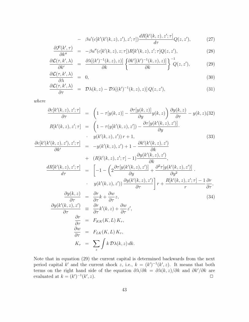
− βu′(c[k′(k′(k, z), z′), z′; τ ])dR[k′(k, z), z′; τ ]

dτQ(z, z′), (27)

∂F(k′, τ)

∂k′′= −βu′′(c[k′(k, z), z; τ ])R[k′(k, z), z′; τ ]Q(z, z′), (28)

∂L(τ, k′, λ)

∂k′=

∂λ[(k′)−1(k, z), z)]

∂k

{∂k′[(k′)−1(k, z), z)]

∂k

}−1

Q(z, z′), (29)

∂L(τ, k′, λ)

∂λ= 0, (30)

∂L(τ, k′, λ)

∂τ= Dλ(k, z)−Dλ[(k′)−1(k, z), z)] Q(z, z′), (31)

where

∂c[k′(k, z), z′; τ ]

∂τ=

(1− τ [y(k, z)]− ∂τ [y(k, z)]

∂yy(k, z)

)∂y(k, z)

∂τ− y(k, z),(32)

R[k′(k, z), z′; τ ] =

(1− τ(y[k′(k, z), z′])− ∂τ [y(k′(k, z), z′)]

∂y·

· y(k′(k, z), z′)) r + 1, (33)

∂c[k′(k′(k, z), z′), z′; τ ]

∂k′= −y(k′(k, z), z′) + 1− ∂k′(k′(k, z), z′)

∂k

+ (R[k′(k, z), z′; τ ]− 1)∂y(k′(k, z), z′)

∂k,

dR[k′(k, z), z′; τ ]

dτ=

[−1−

(2∂τ [y(k′(k, z), z′)]

∂y+

∂2τ [y(k′(k, z), z′)]∂y2

·

· y(k′(k, z), z′))∂y(k′(k, z), z′)

∂τ

]r +

R[k′(k, z), z′; τ ]− 1

r

∂r

∂τ,

∂y(k, z)

∂τ=

∂r

∂τk +

∂w

∂τz, (34)

∂y(k′(k, z), z′)∂τ

≡ ∂r

∂τk′(k, z) +

∂w

∂τz′,

∂r

∂τ= FKK(K,L) Kτ ,

∂w

∂τ= FLK(K, L) Kτ ,

Kτ =∑

z

∫kDλ(k, z) dk.

Note that in equation (29) the current capital is determined backwards from the nextperiod capital k′ and the current shock z, i.e., k = (k′)−1(k′, z). It means that bothterms on the right hand side of the equation ∂λ/∂k = ∂λ(k, z)/∂k and ∂k′/∂k areevaluated at k = (k′)−1(k′, z). 2

43

References

Aiyagari, R. S. (1995). Optimal capital income taxation with incomplete markets, bor-

rowing constraints, and constant discounting. Journal of Political Economy 103,

1158–1175.

Auerbach, A. J. and L. J. Kotlikoff (1987). Dynamic Fiscal Policy.

Bohacek, R. and M. Kejak (2002). Projection methods for economies with heteroge-

neous agents. CERGE-EI Working Paper .

Bohacek, R. and M. Kejak (2004). On the optimal dynamic tax schedule. CERGE-EI

Working Paper .

Chamley, C. (1986). Optimal taxation of capital income in general equilibrium with

infinite lives. Econometrica 54 (3), 607–622.

Conesa, J. C. and D. Krueger (2004). On the optimal progressivity of the income tax

code. Mimeo, Universitat Pompeu Fabra.

Diaz-Jimenez, J., V. Quadrini, and J. V. Rios-Rull (1997, Spring). Dimensions of

inequality: Facts on the u.s. distribution of earnings, income, and wealth. Federal

Reserve Bank of Minneapolis Quarterly Review .

Domeij, D. and J. Heathcote (2004). On the distributional effects of reducing capital

taxes. International Economic Review 45 (2), 523–554.

Garcia-Mila, T., A. Marcet, and E. Ventura (1995). Supply side interventions and

redistributions. Working Paper UPF 115.

Golosov, M., N. R. Kocherlakota, and O. Tsyvinski (2003). Optimal indirect and

capital taxation. Review of Economic Studies 70, 569–587.

Gouveia, M. and R. Strauss (1994). Effective federal individual income tax functions:

An exploratory empirical analysis. National Tax Journal (47), 317–339.

Heaton, J. and D. Lucas (1996). Evaluating the effects of incomplete markets on risk

sharing and asset pricing. Journal of Political Economy 104 (3), 443–487.

Judd, K. L. (1985). Redistributive taxation in a simple perfect foresight model. Jour-

nal of Public Economics 28, 59–83.

Judd, K. L. (1992). Projection methods for solving aggregate growth models. Journal

of Economic Theory 58, 410–452.

Judd, K. L. (1998). Numerical Methods in Economics. Cambridge, MA: MIT Press.

44

Kamien, M. I. and N. L. Schwartz (1991). Dynamic Optimization: The Calculus Of

Variations and Optimal Control in Economics and Management (2nd ed.). New

York: North-Holland.

Klein, P. and J.-V. Rios-Rull (2004). Time-consistent optimal fiscal policy. Interna-

tional Economic Review 44 (4), 1217–1245.

Kocherlakota, N. R. (2003). Zero expected wealth taxes: A mirrless approach to

dynamic optimal taxation.

Kydland, F. and E. C. Prescott (1977). Rules rather than discretion: the inconsistency

of optimal plans. Journal of Political Economy 84, 473–491.

Lucas, Jr., R. E. (1990). Supply-side economics: An analytical review. Oxford Eco-

nomic Papers (42), 293–316.

Mirrlees, J. (1971). An exploration in the theory of optimum income taxation. Review

of Economic Studies 38, 175–208.

Mirrlees, J. (1976). Optimal tax theory: A synthesis. Journal of Public Economics 6,

327–358.

Prescott, E. C. (1986). Theory ahead of business cycle measurement. Carnegie-

Rochester Conference Series on Public Policy 25, 11–44.

Quah, D. (2003). One third of the world’s growth and inequality. In T. Eicher and

S. Turnovsky (Eds.), Growth and Inequality: Issues and Policy Implications, Cam-

bridge. MIT Press.

Ramsey, F. P. (1927). A contribution to the theory of taxation. The Economic Jour-

nal 37, 47–61.

Saez, E. (2002). Optimal progressive capital income taxes in the infinite horizon

model. NBER Working Paper 9046 .

Stokey, N. L., R. E. Lucas, Jr., and E. C. Prescott (1989). Recursive Methods in

Economic Dynamics. Cambridge: Harvard University Press.

Storesletten, K., C. Telmer, and A. Yaron (1999). Asset pricing with idiosyncratic

risk and overlapping generations. Mimeo, Carnegie Mellon University .

Tauchen, G. and R. Hussey (1991). Quadrature-based methods for obtaining approx-

imate solutions to nonlinear asset pricing models. Econometrica 59, 371–396.

Ventura, G. (1999). Flat tax reform: A quantitative exploration. Journal of Economic

Dynamics and Control 23, 1425–1458.

45

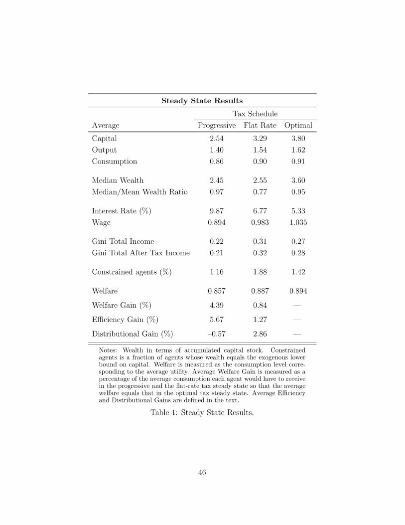
Steady State Results

Tax Schedule

Average Progressive Flat Rate Optimal

Capital 2.54 3.29 3.80

Output 1.40 1.54 1.62

Consumption 0.86 0.90 0.91

Median Wealth 2.45 2.55 3.60

Median/Mean Wealth Ratio 0.97 0.77 0.95

Interest Rate (%) 9.87 6.77 5.33

Wage 0.894 0.983 1.035

Gini Total Income 0.22 0.31 0.27

Gini Total After Tax Income 0.21 0.32 0.28

Constrained agents (%) 1.16 1.88 1.42

Welfare 0.857 0.887 0.894

Welfare Gain (%) 4.39 0.84 —

Efficiency Gain (%) 5.67 1.27 —

Distributional Gain (%) –0.57 2.86 —

Notes: Wealth in terms of accumulated capital stock. Constrainedagents is a fraction of agents whose wealth equals the exogenous lowerbound on capital. Welfare is measured as the consumption level corre-sponding to the average utility. Average Welfare Gain is measured as apercentage of the average consumption each agent would have to receivein the progressive and the flat-rate tax steady state so that the averagewelfare equals that in the optimal tax steady state. Average Efficiencyand Distributional Gains are defined in the text.

Table 1: Steady State Results.

46

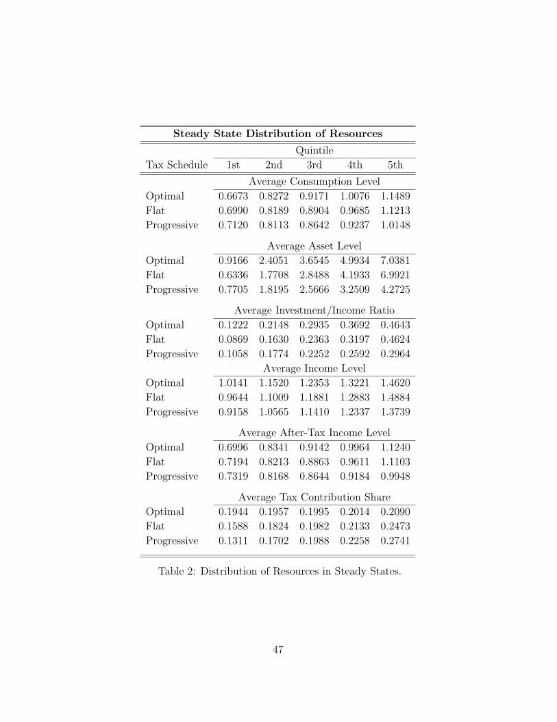
Steady State Distribution of Resources

Quintile

Tax Schedule 1st 2nd 3rd 4th 5th

Average Consumption Level

Optimal 0.6673 0.8272 0.9171 1.0076 1.1489

Flat 0.6990 0.8189 0.8904 0.9685 1.1213

Progressive 0.7120 0.8113 0.8642 0.9237 1.0148

Average Asset Level

Optimal 0.9166 2.4051 3.6545 4.9934 7.0381

Flat 0.6336 1.7708 2.8488 4.1933 6.9921

Progressive 0.7705 1.8195 2.5666 3.2509 4.2725

Average Investment/Income Ratio

Optimal 0.1222 0.2148 0.2935 0.3692 0.4643

Flat 0.0869 0.1630 0.2363 0.3197 0.4624

Progressive 0.1058 0.1774 0.2252 0.2592 0.2964

Average Income Level

Optimal 1.0141 1.1520 1.2353 1.3221 1.4620

Flat 0.9644 1.1009 1.1881 1.2883 1.4884

Progressive 0.9158 1.0565 1.1410 1.2337 1.3739

Average After-Tax Income Level

Optimal 0.6996 0.8341 0.9142 0.9964 1.1240

Flat 0.7194 0.8213 0.8863 0.9611 1.1103

Progressive 0.7319 0.8168 0.8644 0.9184 0.9948

Average Tax Contribution Share

Optimal 0.1944 0.1957 0.1995 0.2014 0.2090

Flat 0.1588 0.1824 0.1982 0.2133 0.2473

Progressive 0.1311 0.1702 0.1988 0.2258 0.2741

Table 2: Distribution of Resources in Steady States.

47

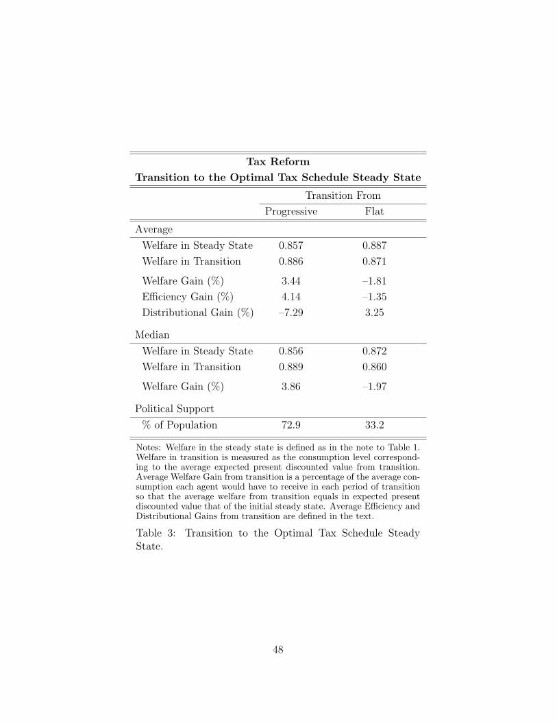
Tax Reform

Transition to the Optimal Tax Schedule Steady State

Transition From

Progressive Flat

Average

Welfare in Steady State 0.857 0.887

Welfare in Transition 0.886 0.871

Welfare Gain (%) 3.44 –1.81

Efficiency Gain (%) 4.14 –1.35

Distributional Gain (%) –7.29 3.25

Median

Welfare in Steady State 0.856 0.872

Welfare in Transition 0.889 0.860

Welfare Gain (%) 3.86 –1.97

Political Support

% of Population 72.9 33.2

Notes: Welfare in the steady state is defined as in the note to Table 1.Welfare in transition is measured as the consumption level correspond-ing to the average expected present discounted value from transition.Average Welfare Gain from transition is a percentage of the average con-sumption each agent would have to receive in each period of transitionso that the average welfare from transition equals in expected presentdiscounted value that of the initial steady state. Average Efficiency andDistributional Gains from transition are defined in the text.

Table 3: Transition to the Optimal Tax Schedule SteadyState.

48

¡¡

¡¡

¡¡

¡¡

¡¡

¡¡

¡¡

¡¡

¡¡

¡¡

¡¡

¡

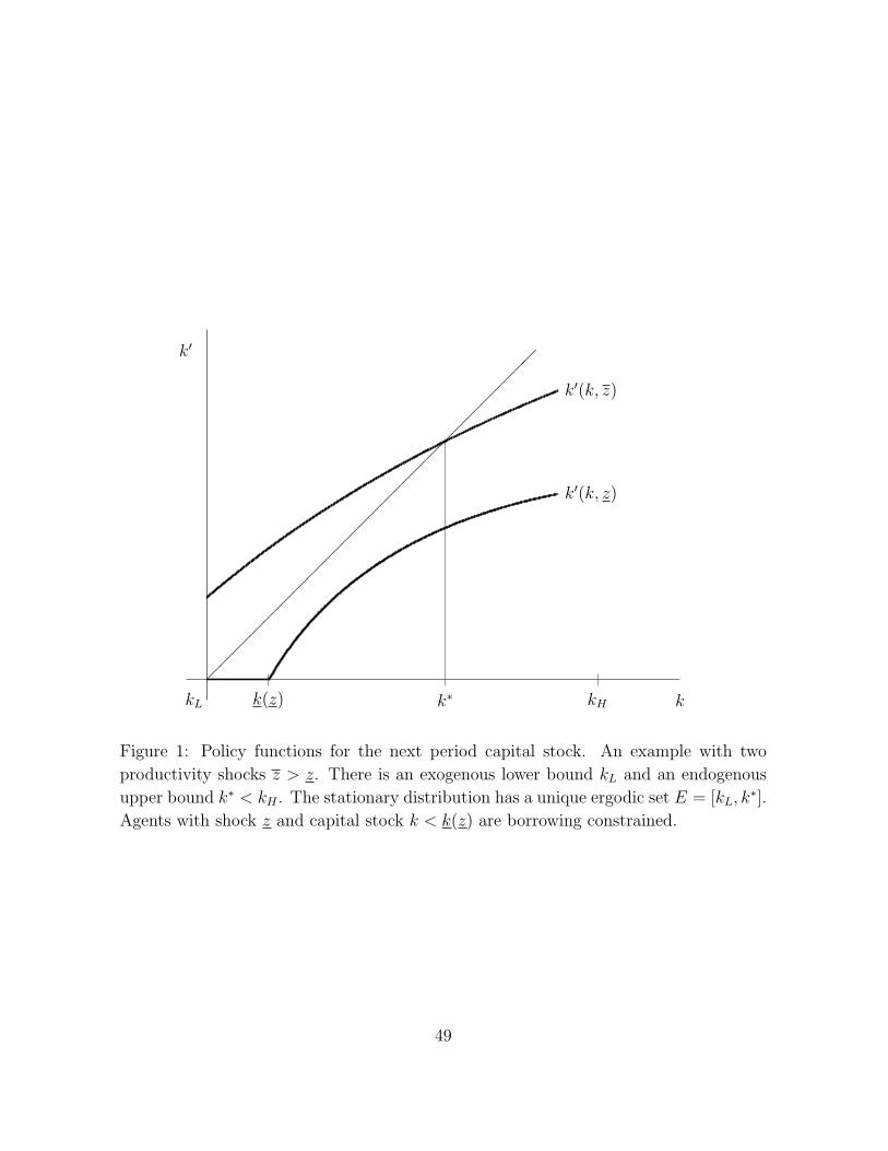
k∗kL k(z)

k′(k, z)

k′(k, z)

k′

kH k

Figure 1: Policy functions for the next period capital stock. An example with two

productivity shocks z > z. There is an exogenous lower bound kL and an endogenous

upper bound k∗ < kH . The stationary distribution has a unique ergodic set E = [kL, k∗].Agents with shock z and capital stock k < k(z) are borrowing constrained.

49

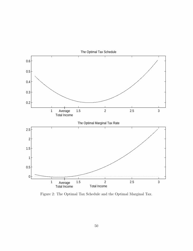
1 1.5 2 2.5 3

0.2

0.3

0.4

0.5

0.6

The Optimal Tax Schedule

IAverage

Total Income

1 1.5 2 2.5 3

0

0.5

1

1.5

2

2.5

The Optimal Marginal Tax Rate

Total Income

IAverage

Total Income

Figure 2: The Optimal Tax Schedule and the Optimal Marginal Tax.

50

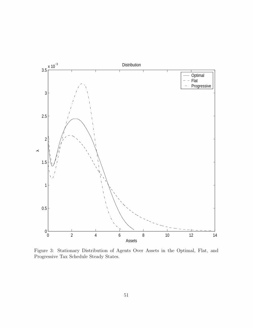
0 2 4 6 8 10 12 140

0.5

1

1.5

2

2.5

3

3.5x 10

−3 Distribution

λ

Assets

OptimalFlatProgressive

Figure 3: Stationary Distribution of Agents Over Assets in the Optimal, Flat, andProgressive Tax Schedule Steady States.

51

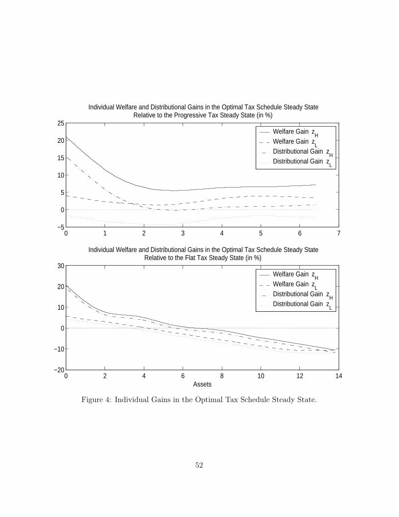
0 1 2 3 4 5 6 7−5

0

5

10

15

20

25

Individual Welfare and Distributional Gains in the Optimal Tax Schedule Steady StateRelative to the Progressive Tax Steady State (in %)

Welfare Gain zH

Welfare Gain zL

Distributional Gain zH

Distributional Gain zL

0 2 4 6 8 10 12 14−20

−10

0

10

20

30

Individual Welfare and Distributional Gains in the Optimal Tax Schedule Steady StateRelative to the Flat Tax Steady State (in %)

Assets

Welfare Gain zH

Welfare Gain zL

Distributional Gain zH

Distributional Gain zL

Figure 4: Individual Gains in the Optimal Tax Schedule Steady State.

52

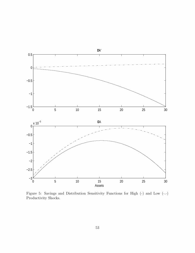
0 5 10 15 20 25 30−1.5

−1

−0.5

0

0.5Dk′

0 5 10 15 20 25 30−3

−2.5

−2

−1.5

−1

−0.5

0x 10

−3 Dλ

Assets

Figure 5: Savings and Distribution Sensitivity Functions for High (-) and Low (-.-)Productivity Shocks.

53

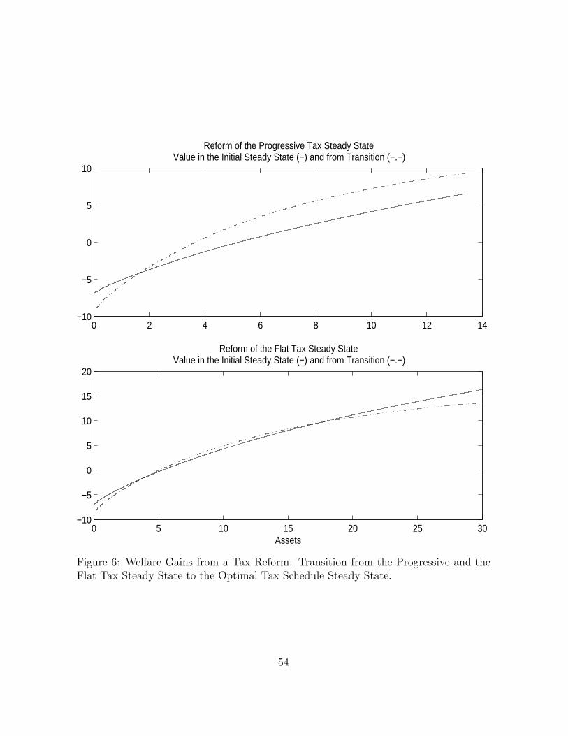
0 2 4 6 8 10 12 14−10

−5

0

5

10

Reform of the Progressive Tax Steady StateValue in the Initial Steady State (−) and from Transition (−.−)

0 5 10 15 20 25 30−10

−5

0

5

10

15

20

Reform of the Flat Tax Steady StateValue in the Initial Steady State (−) and from Transition (−.−)

Assets

Figure 6: Welfare Gains from a Tax Reform. Transition from the Progressive and theFlat Tax Steady State to the Optimal Tax Schedule Steady State.

54

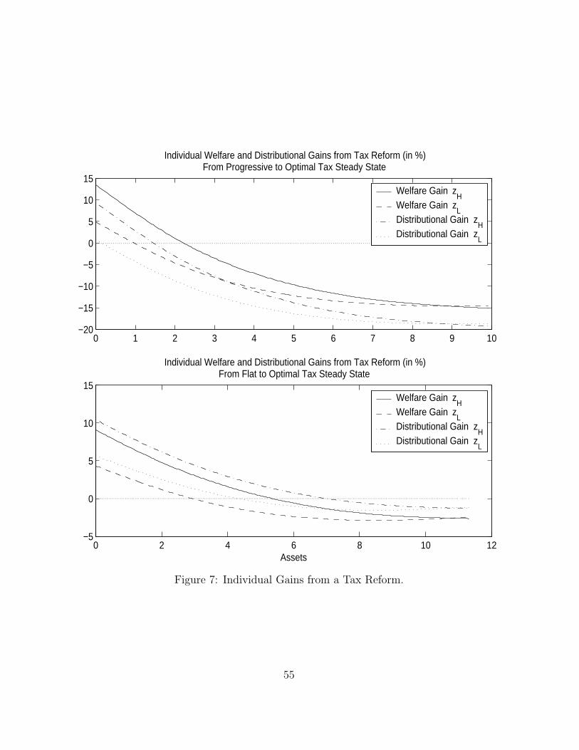
0 1 2 3 4 5 6 7 8 9 10−20

−15

−10

−5

0

5

10

15

Individual Welfare and Distributional Gains from Tax Reform (in %)From Progressive to Optimal Tax Steady State

Welfare Gain zH

Welfare Gain zL

Distributional Gain zH

Distributional Gain zL

0 2 4 6 8 10 12−5

0

5

10

15

Individual Welfare and Distributional Gains from Tax Reform (in %)From Flat to Optimal Tax Steady State

Assets

Welfare Gain zH

Welfare Gain zL

Distributional Gain zH

Distributional Gain zL

Figure 7: Individual Gains from a Tax Reform.

55