KIER DISCUSSION PAPER SERIES

KYOTO INSTITUTE

OF

ECONOMIC RESEARCH

KYOTO UNIVERSITY

KYOTO, JAPAN

Discussion Paper No.952

“The Determinants of Foreign Direct Investment

in Transition Economies: A Meta-Analysis”

Masahiro Tokunaga and Ichiro Iwasaki

November 2016

KIER Discussion Paper Series

November 2016

The Determinants of Foreign Direct Investment in

Transition Economies: A Meta-Analysis

Masahiro Tokunaga† and Ichiro Iwasaki ‡

Abstract: In this paper, we conduct a meta-analysis of studies that empirically examine the

relationship between economic transformation and foreign direct investment (FDI) performance in

Central and Eastern Europe and the former Soviet Union over the past quarter century. More

specifically, we synthesize the empirical evidence reported in previous studies that deal with the

determinants of FDI in transition economies, focusing on the impacts of transition factors. We also

perform meta-regression analysis to specify determinant factors of the heterogeneity among the

relevant studies and the presence of publication selection bias. We find that the existing literature

reports a statistically significant nonzero effect as a whole, and a genuine effect is confirmed for

some FDI determinants beyond the publication selection bias.

JEL classification numbers: E22, F21, P33

Key words: foreign direct investment (FDI), FDI determinants, transition economies, meta-analysis,

publication selection bias

This research was financially supported by a grant-in-aid for scientific research from the Ministry

of Education, Culture, Sports, Science & Technology of Japan (No. 23243032) and Joint Usage and Research Center of the Institute of Economic Research, Kyoto University (FY2016). We thank Tom D. Stanley; Masaaki Kuboniwa; Taku Suzuki; Miklós Szanyi; participants in the 13th EACES biennial conference at Corvinus University, Budapest, September 4−6, 2014; and two anonymous referees for their helpful comments and suggestions on an earlier version of the paper. We also would like to thank Eriko Yoshida for her research assistance and Tammy L. Bicket for her editorial assistance. Needless to say, all remaining errors are solely our responsibility. Iwasaki and Tokunaga (2014) and Iwasaki and Tokunaga (2016) are companion papers to this article and present meta-analyses of macroeconomic growth-enhancing effects and firm-level technology transfer and spillover effects of FDI in transition economies, respectively.

† Faculty of Business and Commerce, Kansai University, 3-3-35 Yamate-cho, Suita City, Osaka 564-8680, JAPAN; E-mail: t030032@kansai-u.ac.jp

‡ Institute of Economic Research, Hitotsubashi University, 2-1 Naka, Kunitachi City, Tokyo 186-8603, JAPAN; E-mail: iiwasaki@ier.hit-u.ac.jp

1

1. Introduction

The economics of transition from a socialist economy to a market economy highlights the necessity

of foreign direct investment (FDI) as an additional financial resource in countries with a lack of

savings and driving forces for the restructuring of extremely inefficient Soviet-type command

economies (Lavigne, 1999, Chapter 9). In the economic theory of transition, therefore, inward FDI

has played an important role because it is considered critical for both economic growth and

structural change (Okafor and Webster, 2016). Although researchers have been divided about the

contribution of inward FDI to economic growth, most of the literature shows that foreign capital

inflows and the advance of multinational enterprises (MNEs) played extremely significant roles in

the restructuring process that began in earnest with the collapse of the Berlin Wall in November

1989 toward the establishment of a capitalist market economy in Central and Eastern Europe (CEE)

and the former Soviet Union (FSU).

In the early transitional period, however, due to the deep-seated skepticism of foreign investors

and firms toward the perspective of the former socialist bloc involved in the serious economic crisis,

foreign investment in this region generally fell far short of expectations throughout the 1990s,

except in Hungary and a few other countries bordering the European Union (EU), each of which

was very active in structural reforms and economic liberalization. In addition, most foreign capital

that had been invested during this period was either spent to acquire state-owned assets and was,

thus, absorbed in the national treasury or was used for portfolio investment. Accordingly, the

overall impact on real economies was minor. The situation surrounding foreign investment changed

substantially after the turn of the century. Among the many factors that encouraged capital inflow

into the CEE and FSU countries during the 2000s, the following are considered to be especially

noteworthy: remarkable progress toward a market economy that resulted in the belief that a return

to the old regime would never occur in the region; a redefinition of these transition economies as

emerging markets against the background of a dramatic business recovery; and the psychological

effects on foreign investors and MNEs that stemmed from the accelerating globalization of the

world economy. Consequently, the accumulated foreign direct investment (FDI) in the CEE and

FSU countries from 1989 to 2014 had a value of US $1.55 trillion, of which approximately 90%

was concentrated in the first ten years of the new century.1 This high concentration of FDI into the

transition economies demonstrates vigorous cross-border capital movement in this period.

From early on, the literature of transition economies has focused attention on the potential for

FDI to play a significant role in the economic reconstruction of the CEE and FSU countries.

Researchers started publishing the results of their full-scale empirical analyses in academic journals

in the mid-1990s (e.g., Meyer, 1995; Wang and Swain, 1995; Lansbury et al., 1996). However,

1 For further information on FDI in the region, see Appendix A.

2

because of the above-mentioned sluggish foreign investment in the early phase of the transition,

combined with various technical constraints such as limited data availability and accessibility,

studies on FDI in the transition economies were far from adequate in terms of both quality and

quantity throughout the 1990s. This sense of inadequacy was greatly dispelled by vigorous research

activity during the 2000s, and now it is not an exaggeration to say that FDI has been elevated to a

position as one of the most important research topics in the field of transition economics.

Now that pertinent empirical studies are considered to be well established, one can ask what

kind of empirical results the existing literature presents as a whole, specifically, whether these

results are sufficient for identifying any true effect and whether any intentional bias in the

publication of the studies or a so-called “publication selection bias” exists. In this paper, we will

provide some answers to these questions by conducting a meta-analysis of studies that empirically

examine the relationship between economic transformation and FDI in the CEE and FSU region

over the past quarter century. While studies of FDI in transition economies encompass diversified

research topics with various theoretical backgrounds and, thus, research methodologies, any

meta-analysis requires a certain number of studies reporting empirical results that are eligible for

the synthesis of estimates and/or the meta-regression analysis (MRA) of heterogeneity among

studies. In light of the development of relevant studies this far, therefore, we can conduct a

meta-analysis focusing on the study of FDI determinants in transition economies, for which a

comparatively large volume of empirical results has been accumulated. This also enables us to

compare the FDI-inducing effect of economic transition with those of other traditional or gravity

models’ FDI determinants to indicate the extent to which transition economy-specific factors have

contributed to FDI performances in the CEE and FSU region. In this regard, this paper will

contribute greatly to deepening our understanding of the relationship between the economic

transformation process and FDI performance in the emerging European economies.

Meta-analyses concerning studies of transition economies remain inadequate, as do those of

FDI determinants in general economies. Eleven systematic reviews or meta-analyses have focused

on relevant studies of transition economies. Among those, Djankov and Murrell (2002) was a

pioneering work that reviewed the empirical literature on enterprise restructuring in transition

economies in a quantitative way; Estrin et al. (2009) followed Djankov and Murrell (2002),

focusing on the effects of privatization and ownership change during the transition period; Iwasaki

(2007) further provided evidence concerning the effects of corporate governance structure through

a comprehensive survey of the literature on the internal structure of Russian corporations. Then

Hanousek et al. (2011) and Iwasaki and Tokunaga (2014, 2016) reviewed a large body of findings

regarding the effects of FDI on transition economies. The remaining five studies are outlined as

follows: Égert and Halpern (2006) and Velickovskia and Pugh (2011) conducted a meta-analysis of

the determinants of the foreign exchange rate; Fidrmuc and Korhonen (2006) devoted themselves

3

to analyzing the literature of the business cycle pattern; Babecký and Campos (2011) and Babecky

and Havranek (2014) reviewed the relationship between structural reforms and economic growth

with meta-analysis techniques. In the meantime, meta-analyses concerning studies of FDI

determinants in general works touch entirely on the impact of taxation on FDI (see de Mooij and

Ederveen (2003, 2008) and Feld and Heckemeyer (2011)); among works selected by our

meta-analysis, Bellak and Leibrecht (2006, 2007a, 2007b, 2009) and Overesch and Wamser (2010)

share those same research interests.

The remainder of this paper is organized as follows: The next section describes our

methodology for literature selection and meta-analysis. Section 3 gives an overview of the studies

selected for meta-analysis. Section 4 demonstrates our synthesis of the collected estimates. Section

5 performs meta-regression analysis to explore the heterogeneity observed between studies. Section

6 assesses the publication selection bias. Section 7 summarizes our major findings and concludes

the paper.

2. Methodology of Literature Selection and Meta-analysis

In this section, we describe our methods of selecting and coding relevant studies and for

meta-analysis based on the empirical evidence collected. Unlike Hanousek et al. (2011) and

Iwasaki and Tokunaga (2014, 2016), studies that deal with direct and indirect FDI effects, this

paper focuses on empirical studies of FDI determinants in transition economies. Furthermore, as

compared with relevant literature of the past, the methodology for the meta-analysis used in this

paper is more comprehensive, in accordance with the guidelines advocated by Stanley and

Doucouliagos (2012).

In order to identify studies related to FDI in the CEE and FSU countries as a base collection, we

first searched the EconLit and Web of Science databases for research works that had been

registered in the 27 years from 1989 to 2015 that contained a combination of two terms including

one from foreign direct investment, FDI, or multinational enterprise and another one from

transition economies, Central Europe, Eastern Europe, the former Soviet Union, or the respective

names of each CEE and FSU country.2 From approximately 550 studies that we found at this stage,

we actually obtained more than 380 studies, or about 70% of the total. We also searched the

references in these 380 studies and obtained approximately 90 additional papers. As a result, we

collected approximately 470 studies.

These 470 studies included various papers other than empirical studies on FDI determinants in

transition economies. Hence, as the next step, we closely examined the contents of these works and

narrowed the literature list to those containing estimates that could be subjected to meta-analysis in

2 The last literature search using these databases was carried out in March 2016.

4

this paper. In the next section, we report the results of our literature selection in detail. During this

process, we decided to exclude all unpublished research works. According to Doucouliagos, Haman,

and Stanley (2012), unpublished working papers might present estimates that are not final;

moreover, these manuscripts are more likely to be insufficient since they had not yet gone through

the peer review process. In our judgment, the same concerns apply to unpublished works we

obtained for this study. Another reason to exclude unpublished works is that we use the quality

level of each paper that we evaluate, based on external indicators like as journal’s rakings, as a

weight for a combination of statistical significance levels and as an analytical weight or a

meta-independent variable for the MRA. In addition, the following facts also motivate us to take

this measure: First, the number of working papers is not large in our case. Second, these

unpublished works are not heavily concentrated in recent years. The latter fact led us to decide that

there is no particular concern of overlooking the latest research results due to their exclusion.

For this study, we adopted an eclectic coding rule to simultaneously mitigate the following two

selection problems: The first is the arbitrary-selection problem caused by data collection in which

the meta-analyst selects only one estimate per study. The second is over-representation caused by

data collection in which all estimates are taken from every study without any conditions. More

specifically, we do not necessarily limit the selection to one estimate per study, but multiple

estimates are collected if, and only if, we can recognize notable differences from the viewpoint of

empirical methodology in at least one item of the target regions/countries, data type, regression

equation, estimation period, and estimator. Hereafter, K denotes the total number of collected

estimates (k = 1, 2, . . ., K).

Next, we outline the meta-analysis to be conducted in the following sections. In this study, we

employ the partial correlation coefficient (PCC) and the t value to synthesize the collected

estimates. The PCC is a measure of the association of a dependent variable and the independent

variable in question when other variables are held constant. The PCC is calculated in the following

equation:

, 1

where tk and dfk denote the t value and the degree of freedom of the k-th estimate, respectively. The

standard error (SE) of rk is given by 1 ⁄ .3

3 A benefit of the PCC is that it makes it easier to compare and synthesize collected estimates of

independent variables with definitions or units that differ. On the other hand, a flaw of the PCC is that its distribution is not normal when the coefficient is close to -1 or +1 (Stanley and

Doucouliagos, 2012, p. 25). Fisher’s z-transformation ln is the best known solution

to this problem. As in overall economic studies, the PCC of each estimate used for our meta-analysis was rarely observed to be close to the upper or lower limit; thus, we used the PCC

5

The following method is used to synthesize PCCs. Suppose that there are K estimates. Here, the

PCC of the k-th estimate is labeled as rk, and the corresponding population and standard deviation

are labeled as θk and Sk, respectively. We assume that θ1 = θ2 = … = θK = θ, implying that each

study in a meta-analysis estimates the common underlying population effect and that the estimates

differ only by random sampling errors. An asymptotically efficient estimator of the unknown true

population parameter θ is a weighted mean by the inverse variance of each estimate:

, 2

where 1⁄ and . The variance of the synthesized partial correlation is given by 1 ∑⁄ .

This is the meta fixed-effect model. Hereafter, we denote estimates of the meta fixed-effect

model using . To utilize this method of synthesizing PCCs, we need to confirm that the

estimates are homogeneous. A homogeneity test uses the statistic:

~ 1 , 3

which has a chi-square distribution with N-1 degrees of freedom. The null hypothesis is rejected if Qr exceeds the critical value. In this case, we assume that heterogeneity exists among the studies and adopt a random-effects model that incorporates the sampling variation due to an underlying population of effect sizes as well as the study-level sampling error. If the deviation between

estimates is expressed as 2 , the unconditional variance of the k-th estimate is given by

. In the meta random-effects model, the population θ is estimated by replacing the weight

wk with the weight 1⁄ in Eq. (2).4 For the between-studies variance component, we use

the method of moments estimator computed by the next equation using the value of the homogeneity test statistic Qr obtained from Eq. (3):

1

∑ ∑ ∑. 4

Hereafter, we denote the estimates of the meta random-effects model as .

Following the precedent of Djankov and Murrell (2002), we combine t values using the next

equation:5

~ 0,1 . 5

as calculated in Eq. (1).

4 This means that the meta fixed-effect model is a special case based on the assumption that 02 . 5 Iwasaki (2007) and Wooster and Diebel (2010) also adopted this method of combining the t

values.

6

Here, wk is the weight assigned to the t value of the k-th estimate. As the weight wk in Eq. (5),

we utilize a 10-point scale to mirror the quality level of each relevant study 1 10 . More

concretely, if the study in consideration is a journal article, the quality level is determined on the

basis of the economic journal’s ranking and its impact factor. For either a book or a book chapter,

the quality level is determined based on the presence or absence of a peer review process and

literature information, such as the publisher.6 Moreover, we report not only the combined t value

weighted by the quality level of the study but also the unweighted combined t value

obtained according to the following equation:

√ ~ 0,1 . 6

By comparing these weighted and unweighted combined t values, we examine the relationship

between the quality level and the level of statistical significance reported by each study.

As a supplemental statistic for evaluating the reliability of the above-mentioned combined t

value, we also report Rosenthal’s fail-safe N (fsN) as computed by the next formula:7

0.05∑1.645

. 7

After synthesizing the collected estimates, we conduct an MRA to explore the factors causing

heterogeneity among selected studies. To this end, we estimate the meta-regression model:

, 1,⋯ , , 8

where yk is the PCC or the t value of the k-th estimate; xkn denotes a meta-independent variable that

captures all usable characteristics of an empirical study and explains its systematic variation from

other empirical results in the literature; βn denotes the meta-regression coefficient to be estimated;

and ek is the meta-regression disturbance term (Stanley and Jarrell, 2005).

When selecting an estimator for meta-regression models, we should pay the most attention to

heterogeneity among selected studies. It is especially true in our case, where multiple estimates are

to be collected from one study. Therefore, we perform an MRA using the following six estimators:

the cluster-robust ordinary least squares (OLS) estimator, which clusters the collected estimates by

study and computes robust standard errors; the cluster-robust weighted least squares (WLS)

6 For more details on the method of evaluating the quality level, see Appendix B. 7 Rosenthal’s fail-safe N denotes the number of studies with the average effect size equal to zero,

which needs to be added in order to bring the combined probability level of all the studies to the standard significance level to determine the presence or absence of effect. The larger value of fsN in Eq. (7) means the more reliable estimation of the combined t value. For more details, see Mullen (1989, Chapter 6) and Stanley and Doucouliagos (2012, pp. 73-74).

7

estimator, which uses either the above-mentioned quality level of the study, the number of

observations (N) or the inverse of the standard error (1/SE) as an analytical weight; the multilevel

mixed effects restricted maximum likelihood (RML) estimator; and the unbalanced panel

estimator.8 In this way, we check the statistical robustness of coefficient βn.

Testing for publication selection bias is an important issue on par with the synthesis of estimates

and meta-regression of between-study heterogeneity. In this paper, we examine this problem by

using the funnel plot and the Galbraith plot as well as by estimating the meta-regression model that

is designed especially for this purpose.

The funnel plot is a scatter plot with the effect size (the PCC in this paper) on the horizontal

axis and the precision of the estimate (1/SE in this case) on the vertical axis. In the absence of

publication selection, effect sizes reported by independent studies vary randomly and

symmetrically around the true effect. Moreover, according to statistical theory, the dispersion of

effect sizes is negatively correlated with the precision of the estimate. Therefore, the shape of the

plot must look like an inverted funnel. This means that if the funnel plot is not bilaterally

symmetrical but is deflected to one side, an arbitrary manipulation of the study area in question is

suspected, in the sense that estimates in favor of a specific conclusion (i.e., estimates with an

expected sign) are more frequently published (type I publication selection bias).

Meanwhile, the Galbraith plot is a scatter plot with the precision of the estimate (1/SE in this

paper) on the horizontal axis and the statistical significance (the t value in this case) on the vertical

axis. We use this plot for testing another arbitrary manipulation in the sense that estimates with

higher statistical significance are more frequently published, irrespective of their sign (type II

publication selection bias). In general, the statistic, | the thestimate thetrueeffect / |,

should not exceed the critical value of ±1.96 by more than 5% of the total estimates. In other

words, when the true effect does not exist and there is no publication selection, the reported t values

should vary randomly around zero, and 95% of them should be within the range of ±1.96. The

Galbraith plot tests whether the above relationship can be observed in the statistical significance of

the collected estimates, thereby identifying the presence of type II publication selection bias. In

addition, for the above reasons, the Galbraith plot is also used as a tool for testing the presence of a

nonzero effect.9

In addition to the two scatter plots, we also report estimates of the meta-regression models,

which have been developed to examine in a more rigorous manner the two types of publication

8 This refers to cluster-robust random-effects and fixed-effects estimators. The unbalanced panel

estimator is selected on the basis of the Hausman test of the random-effects assumption. We also report the results of the Breusch-Pagan test for testing the null hypothesis that the variance of the individual effects is zero in order to question whether the panel estimation itself is appropriate. We set the critical value for both of these model specification tests at a 10% level of significance.

9 For more details, see Stanley (2005) and Stanley and Doucouliagos (2009).

8

selection bias and the presence of the true effect.

We can test for type I publication selection bias by regressing the t value of the k-th estimate on

the inverse of the standard error (1/SE) using the following equation:

1⁄ , 9

thereby testing the null hypothesis that the intercept term β0 is equal to zero.10 In Eq. (9), vk is the

error term. When the intercept term β0 is statistically significantly different from zero, we can

interpret that the distribution of the effect sizes is asymmetric. For this reason, this test is called the

funnel-asymmetry test (FAT). Meanwhile, type II publication selection bias can be tested by

estimating the next equation, where the left side of Eq. (9) is replaced with the absolute t value:

| | 1⁄ 10

thereby testing the null hypothesis of β0 = 0 in the same way as does the FAT.

Even if there is a publication selection bias, a genuine effect may exist in the available empirical

evidence. Stanley and Doucouliagos (2012) propose examining this possibility by testing the null

hypothesis that the coefficient β1 is equal to zero in Eq. (9). The rejection of the null hypothesis

implies the presence of a genuine effect. They call this test the precision-effect test (PET).

Moreover, they also state that an estimate of the publication-bias-adjusted effect size can be

obtained by estimating the following equation that has no intercept:

1⁄ , 11

thereby obtaining the coefficient β1. This means that if the null hypothesis of β1 = 0 is rejected, then

the nonzero effect does actually exist in the literature and the coefficient β1 can be regarded as its

estimate. Stanley and Doucouliagos (2012) call this procedure “the precision-effect estimate with

standard error” (PEESE) approach.11 To test the robustness of the regression coefficient, we

10 Eq. (9) is an alternative model to the following meta-regression model that takes the effect size as

the dependent variable and the standard error as the independent variable:

effectsize 9b More specifically, Eq. (9) is obtained by dividing both sides of the equation above by the standard

error. The error term in Eq. (9b) does not often satisfy the assumption of being i.i.d.

(independent and identically distributed). In contrast, the error term in Eq. (9), ⁄ , is normally distributed; thus, it can be estimated by OLS. Type I publication selection bias can also be detected by estimating Eq. (9b) using the WLS estimator with the inverse of the squared

standard error 1⁄ as the analytical weight and, thereby, testing the null-hypothesis of β0 = 0

(Stanley, 2008; Stanley and Doucouliagos, 2012, pp. 60-61). 11 We can see that the coefficient β1 in Eq. (11) may become the estimate of the

publication-selection-bias-adjusted effect size in light of the fact that the following equation is obtained when both sides of Eq. (11) are multiplied by the standard error:

Effectsize . 11b

9

estimate Eqs. (9) to (11) above using not only the OLS estimator but also the cluster-robust OLS

estimator and the unbalanced panel estimator,12 both of which treat possible heterogeneity among

the studies.

To summarize, to test for publication selection bias and the presence of a genuine empirical

effect, we take the following four steps: First, we test the type I publication selection bias by

estimating Eq. (9) to examine the FAT and the type II publication selection bias by estimating Eq.

(10). Second, regardless of the outcome of the publication selection bias tests, we conduct the PET

to test the existence of a genuine effect in the collected estimates beyond possible contamination

from publication bias. Third, in cases where the null hypothesis of the PET is rejected, we obtain an

estimate of β1 in Eq. (11) using the PEESE approach. Finally, if β1 in Eq. (11) is statistically

significantly different from zero, we report β1 as the estimate of the

publication-selection-bias-adjusted effect size. In cases where the null hypothesis of PET is

accepted, we judge that the literature in question fails to provide sufficient evidence to capture the

genuine effect.13

3. Overview of Selected Studies for Meta-analysis

In this section, we give a comprehensive review of the selected studies for a meta-analysis of the

determinants of FDI in the CEE and FSU countries during the transition period. Among various key

FDI-enhancing factors being discussed so far, a central preoccupation of scholars and policy

makers in the region is the extent to which FDI inflow has been influenced by market economy

reforms such as liberalization, enterprise restructuring, competition policy, and privatization. As

mentioned above, some empirical works were in place by the mid-1990s, and all of these studies

found a positive correlation between FDI performance and market economy reforms related to the

processes of economic transition that were represented by transition indicators of the European

Bank for Reconstruction and Development (EBRD), among other things (Lankes and Venables,

1996; Lansbury et al., 1996; Selowsky and Martin, 1997; EBRD, 1998, Chapter 4). Then, a rapidly

increasing FDI inflow in the ensuing years and the growing availability of statistical data for

When directly estimating Eq. (11b), the WLS method, with 1⁄ as the analytical weight, is

used (Stanley and Doucouliagos, 2012, pp. 65–67). 12 To estimate Eqs. (9) and (10), we use either the cluster-robust random-effects estimator or the

cluster-robust fixed-effects estimator, according to the results of the Hausman test of the random-effects assumption. With regard to Eq. (11), which does not have an intercept term, we report the random-effects model estimated by the maximum likelihood method.

13 As mentioned above, we basically follow the FAT–PET–PEESE approach advocated by Stanley and Doucouliagos (2012, pp. 78–79) as the test procedures for publication selection. However, we also include the test of type II publication selection bias using Eq. (10) as our first step because this kind of bias is very likely in the literature regarding FDI in transition economies.

10

econometric analysis enabled researchers to accelerate their study of FDI determinants in the

transition economies, a large part of which drew the conclusion that more progress in the economic

transition led to greater FDI received.

In accordance with the method of literature selection described in the previous section, we

selected a total of 69 studies that contain estimates suitable for our meta-analysis. Table 1 lists the

selected studies. Note that we removed those studies that, first, do not provide empirical results in

quantitative way, such as descriptive studies specifically; second, involve only one explanatory

variable in simple regression models; third, adopt binary dependent variables with probit and/or

logit estimators, of which the explanatory variables’ effect sizes are not comparable to those of

linear regression models 14 ; and fourth, focus spatially-limited areas or specific industrial

sub-sectors in a host country, of which the research design seems to be fundamentally different

from those of country-level studies.

Although, even in the early 1990s, there was academic work that reviewed trends in FDI

inflows to the CEE and FSU countries using official investment statistics, full-scale empirical

studies drawing upon an econometric method were extremely limited in the 1990s. However, as

Table 1 shows, the 2000s saw an increasing number of econometric papers on FDI determinants in

the region, which demonstrates the increasing popularity of FDI studies among researchers of

transition economies. This was caused by ballooning FDI in the region as well as by the business

community’s raising the prospect that the new accession of transition-advanced countries to the EU

would lead to a review of the investment strategies of MNEs, resulting in an overall restructuring of

business operations at the Pan-European level.15 Therefore, the main areas of research interest have

been the ten CEE countries that joined the EU in 2004 and 2007.

This table also tells us that non-EU CEE countries with only one-eighth the cumulative FDI, as

compared to the new EU membership states (see Appendix A), and FSU countries, excluding the

Baltics, with less opportunity to participate in the process of EU accession despite high FDI

performance or potential, are moved out of the research object inter alia among the empirical

studies. An exception is Croatia, which joined the EU in 2013. Deichmann (2013) and Derado

(2013) are good examples of works driven by the perspective of a country’s EU accession process.

Also, recent studies try to fill the knowledge gap, focusing on the determinants of FDI location in

Southeastern Europe or the Balkans (Dauti, 2015b; Estrin and Uvalic, 2014; Hengel, 2011). On the

whole, except for Döhrn (2000) and Jensen (2002), who do not report the composition of FDI

recipients, the total number of host country observations is 833, of which 60.1% (501 observations) 14 See Stanley and Doucouliagos (2012, pp. 16–17) for more details. 15 To cite an example, Japanese firms have so radically changed the pattern of direct investment in

Europe with increasing FDI into the new membership states that they built more greenfield manufacturing plants in the eastern part of Europe in the first half of the 2000s than in their western counterparts (Ando, 2006).

11

deal with CEE EU countries. Meanwhile, the share of non-EU CEE countries and FSU countries,

excluding the three Baltic states, account for only 14.2% (118 observations) and 18.4% (153

observations), respectively. A few host countries outside of Europe are included in the table because

Wang and Swain (1997) and Jiménez (2011) incorporate non-European emerging markets into their

panels in an undetachable way.

Empirical analysis in the selected studies above covers the 23 years from 1989 to 2011 as a

whole.16 The average estimation period of collected estimates is 10.6 years (median: 10, standard

deviation: 4.2). 37 studies employ the total FDI model with all FDI received from the world as a

dependent variable, while 30 studies rely on the bilateral FDI model that uses an amount of FDI

from a specific home country as a dependent variable. The remaining two, i.e., Demekas et al.

(2007) and Iwasaki and Suganuma (2009), estimate both models. As Table 1 shows, all home

countries are included in a majority of the studies using the total FDI model; in other words, they

use the total value of FDI from the rest of the world in their explanation. On the other hand, most

studies using the bilateral FDI model are based on the gravity model and, thus, specify the home

countries so as to detect the effect of the geographical distance between FDI recipients and

suppliers.17 In the table, we can see the recent upward trend in the number of studies adopting the

bilateral model, which reflects the intention of those who have been analyzing FDI determinants in

general to attach more weight to the gravity model as a basic research design. Reflecting the reality

that a large portion of inward FDI to the CEE and FSU countries comes from advanced countries

within the EU, the bilateral FDI model makes Western Europe a main target for analysis. Non-EU

advanced countries (mainly the United States, Japan, and Switzerland) and leading emerging

market economies, including those in the former socialist block (e.g., Hong Kong, Korea, Russia,

and the Visegrad Group countries), are also added to the list of investors in Bandelj (2002, 2008b),

Bevan and Estrin (2004), Deichmann (2010, 2013), and Estrin and Uvalic (2014).

As for data type, studies using panel data make up three-fourths of the total; otherwise they

employ cross-sectional data or rely on time series data in only a limited number of cases. Table 1

shows that many researchers were conducting empirical analyses with cross-sectional data until the

mid-2000s. This is probably due to the limited availability of longitudinal data as well as the

volatility of FDI inflow to the region during the first decade of the transition. Next, the FDI

indicators to be introduced as dependent variables in the left-hand side of regression equations can

be subdivided into seven groups. According to Table 1, the annual net FDI inflow (Type I) is the

most commonly used indicator; 25 of the 69 studies count upon this type of variable. Annual gross

FDI inflow (Type II), cumulative gross FDI value or FDI (including fixed capital) stock (Type III),

16 Only Wang and Swain (1997) include a pre-transition period for their longitudinal data analysis. 17 Note that the bilateral FDI model, without explanatory variables for geographical distance, does

not follow the gravity model in its original meaning.

12

and annual FDI inflow divided by the value added or industrial output to control for the difference

of economic scale within the target countries (Type VI) follow this; approximately a dozen studies

use each type. Other types of FDI variables are each used in three to five studies. The FDI variable

chosen seems to depend both on purely technical considerations and a priori selection of the

specific variables, given the research interest of each study. In the case of the first issue, when one

applies published and widely used FDI datasets that are often extracted from the UNCTADstat,

OECD StatExtracts, the World Economic Outlook database of the IMF, and the World

Development Indicators provided by the World Bank Group, a negative value would come into

being because these datasets express the annual net value of FDI flow or a difference between

inbound FDI and outbound FDI based on the balance of payment statistics of each country, which

poses a serious obstacle to performing log-transformed linear regression. In fact, we have seen a

negative bilateral investment flow in the CEE and FSU countries explicitly during the two financial

crises of the mid-1990s and 2008−2009; in Russia, among others, “capital flight” continues to be a

macroeconomic problem even now, despite its largest FDI volume received in absolute terms.

Besides that, the unevenness of FDI inflow has the potential to make for more noisy relationships

of other flows, such as GDP, to which they are often scaled (Claessens et al., 2000). To avoid this

problem, Garibaldi et al. (2001) use the gross value of FDI inflow without any deduction for

outflow, and Botrić and Škuflić (2006) cite the FDI stock from a direct investment position

database, for example. As for a priori selection of FDI indicators, although not often expressly

stated in the papers, it is highly predictable that the authors of the literature subject to our

meta-analysis prefer a specific FDI variable for their research design and tasks. To give an example,

Overesch and Wamser (2010) argue for the conceptual advantages of the number of investments

(count variable) as a result of location choice by MNEs because an usual form of binary choice

model (to go or not to go) is incapable of taking into account that MNEs often have multiple

affiliates in a host country.

Meanwhile, transition-specific explanatory variables that are incorporated into the right-hand

side of regression equations can be classified according to their contents with six indicators (see

Table 1). As we have mentioned before, in most cases, the selected studies use EBRD transition

indicators and/or their sub-indicators by area as proxies for the extent of the economic

transformation, and, thus, the classification reflects in principle how the EBRD categorizes the

transition process into these indicators.18 However, the privatization indicators stipulated herein

18 Some researchers have been critical and skeptical of an econometric approach to measuring the

FDI-inducing effect of transition from the early stage of market economy reforms; according to Myant and Drahokoupil (2012), a high score in quantified transition indicators does not necessarily imply that an efficient modern economy has been established, as the indicators are based on a narrow concept of private ownership rather than on a broader perspective of economic development that is truly indispensable for transition countries. As was acknowledged both by the

13

include the large- and small-scale privatization indexes provided by the EBRD as well as other

privatization-related variables, such as private sector share and privatization revenues in each

country. Table 1 reveals that studies using these privatization indicators (Type V) as

transition-specific explanatory variables are in the majority, accounting for 22 of the total 42

studies with them. This is understandable in light of the fact that by-bidding direct sales of

state-owned assets was proposed as a way of privatization in the CEE and FSU countries, thereby

dramatically increasing FDI inflow in some cases, as symbolized by Hungary in the 1990s.

Subsequently, eleven papers employ general transition indicators (Type I); those that rely on

liberalization indicators (Type II), enterprise reform indicators (Type III), and competition policy

indicators (Type IV) are in a minority (five or six studies for each), and, interestingly, eighteen

deploy other transition indicators such as trade and forex systems, the efficiency of law institutions,

infrastructure reform, and financial sector reform. This last point would suggest the breadth of

researchers’ understanding of the economic transition or, alternatively, reflect that there is no clear

consensus concerning the essence of the economic transition in the region. Furthermore, as implied

in the average precision (AP) of estimates by studies reported in Table 1, there is no apparent

tendency for their precision to converge in each category of transition-specific explanatory

variables.

The economic literature specifies a broad array of FDI determinants, not only for transition

economies but also for all parts of the world. It has verified that the local market size, often

expressed as the GDP or population of a country, has a positive and statistically significant effect

on FDI performance.19 Papers reviewing empirical and survey studies of the FDI determinants of

the CEE and FSU countries reveal the significance of market size as an incentive for foreign

investment, which has been a consensus among researchers since an early period (Lankes and

EBRD, which formulated transition indicators, and Nicolas Stern, who served as the chief economist in the 1990s, the simple approach to transition indicators leaves out what seems to be important to the functioning of the market economy; even though the state authorities must be sufficiently strong and well organized to secure well-regulated and efficiently operational market mechanisms, these over-arching and basic considerations are reflected only in a limited way in quantifying the economic transformation process in the CEE and FSU countries (Stern, 1997). Therefore, transition indicators show how far an economy has moved from a planned or command regime to a market economy; however, they do not fully indicate how and to what extent a country has worked to carry forward its market reforms. Therefore, Djankov and Murrell (2002)’s warning holds true even now. They noted that the empirical research on transition economies that existed at the time paid little attention to how to make sense of transition in the wider context of economic development.

19 See Chakrabarti (2001) and Eicher et al. (2012) for estimates of FDI determinants at the global level.

14

Venables, 1996; Estrin et al., 1997; Holland et al., 2000).20 Thus, it is meaningful to conduct a

meta-analysis that will synthesize the estimates of the relevant studies with respect to the effect of

economic transition on FDI and compare the FDI-inducing effect of economic transition with those

of other potential FDI determinants to provide a clear-cut picture of the extent to which transition

economy-specific factors have quantitatively influenced these countries’ FDI performances.

The selected empirical studies herein contain various explanatory variables as FDI determinants,

of which some are target variables to be explored and some are controlling variables for

multivariate analysis. Therefore, in addition to the transition variables above, we collected and

categorized the estimates of other variables into nine types (see Table 1).21 Market-related

variables (i.e., market size variables and purchasing power variables) and labor cost variables (both

in level and difference) are often included in controlling for potential FDI determinants to verify the

effect sizes of focused variables. In most, if not all, cases, geographical distance variables are

incorporated into the bilateral FDI model for the reason that we have already discussed in this

section. About one-third of papers introduce trade effect variables in an attempt to determine

whether a relationship between FDI and trade is complementary or substitutional in the cases of the

CEE and FSU countries. Agglomeration effect variables denote that the presence of other foreign

firms is expected to motivate FDI, as in Doytch and Eren’s (2012) clearly formulated research

strategy; in some cases, however, these variables appear as a result of the incorporation of lagged

FDI variables to estimate a dynamic panel model with a theoretical consideration of the equilibrium

20 According to Lefilleur (2008), who reviewed the studies of FDI determinants in the CEE and FSU

countries, however, a growing body of literature reports that local market size does not have a significant effect on FDI in the region. The vote-counting method shows that, whereas all 33 papers published before the year 2000 reported a positive and significant coefficient of its proxy variable, nine of the 25 studies that were published after that year found an insignificant or negative relationship between market size and FDI performance.

21 We exclude corporate income tax-related variables from our meta-analysis, although the impact of corporate taxes, tax incentives, and tax structures on cross-border capital flows is an issue in selected studies such as Beyer (2002), Edmiston et al. (2003), and Bellak and Leibrecht (2006, 2007a, 2007b, 2009). A meta-analysis of FDI and taxation by Feld and Heckemeyer (2011) reported that the tax-rate elasticity of FDI is highly dependent on which index of corporate income tax is adopted for analysis: whereas semi-elasticities based on the statutory tax rate are often statistically non-significant in empirics, those studies that use the bilateral effective average tax rate reveal that semi-elasticities are significant in almost all of the observed cases. This argument is in line with de Mooij and Ederveen’s (2003, 2008), which applies a meta-analysis to the empirical findings on semi-elasticities of the corporate tax base. A series of works by Bellak and Leibrecht tells us that this is also the case for the CEE countries. In our view, it is not appropriate for our research design to synthesize those estimates whose statistical significance is de facto pre-determined when making relevant variables.

15

process of FDI.22 The two remaining potential FDI determinants, resource abundance variables and

EU accession variables, are mainly targeted to the FSU region and the new EU CEE sample,

respectively. Resource-rich FSU countries such as Russia, Kazakhstan, Azerbaijan, and

Turkmenistan seem to attract resource-seeking FDI, and their growing consumer markets, thanks to

oil and gas revenues, would anchor market-seeking FDI there. Meanwhile, whether eastward

enlargement of the EU boosted FDI in the new member countries has, undoubtedly, been one of the

top research agendas in this field.23 In the following sections, we use estimates of these variables to

weight the effect sizes and gauge the statistical significance of all potential FDI determinants,

including transition-specific variables, which are the focus of this paper.

4. Synthesis of Estimates

Figures 1 and 2 illustrate frequency distribution of the PCC and that of the t value of ten

semantically clustered FDI determinants, using 933 estimates collected from the 69 studies listed in

Table 1. Goodness-of-fit testing for each panel indicates that either the PCC or the t value—or

both—is distributed in a nearly normal distribution for six of ten determinants; however, variables

of purchasing power, trade effect, labor cost difference, and resource abundance do not satisfy the

criteria. As for the transition-related variables that are the focus in subsequent sections of this paper,

both the PCC and the t value are distributed with a nearly normal distribution with modes of 0.15

and 1.75, respectively. According to Cohen’s (1988) guidelines of PCC, 29.7% (55 estimates) find

no practical relationship (|r|<0.1) between transition progress and FDI performance in the CEE and

FSU countries, while 48.7% (90 estimates) and the remaining 21.6% (40 estimates) report a small

effect (0.1≤|r|<0.3) and a medium or large effect (0.3≤|r|), respectively. Meanwhile, Panel (b) of the

figure tells us that the estimates of transition-related variables with respective absolute t values that

are equal to or greater than 2.0 account for 55.7% (103 estimates) of the total.

To consider the implications of the integration of empirical results in a more systematic way, we

synthesized the collected estimates of the selected studies using the meta-synthesis methodology

outlined in Section 2. Table 2 indicates the outcome of the integration of all of the estimates

extracted from the whole sample, while Table 3 shows that of estimates restricted solely to

transition-specific explanatory variables. In addition to the overall synthesis results shown on the

top line, both tables also report individual synthesis results, focusing on differences in data types,

model types, types of FDI variable, and types of FDI determinant for Table 2, or of transition

variable for Table 3, in light of the discussion in the previous section.

22 See Carstensen and Toubal (2004) and Michalíková and Galeotti (2010) for more details on this

point. 23 See Iwasaki and Suganuma (2009) for a review of the literature.

16

As shown in column (a) of both tables, which reports the synthesis results of the PCC, the

homogeneity test rejects the null hypothesis in almost every case; thus, the synthesized effect size,

, of the random-effects model is adopted as the reference value. The synthesized PCC of all

estimates (K = 933) is greater than 0.1, with statistical significance at the 1% level, which is almost

twice as high as the effect size of the transition-related variables (K = 185); this suggests that other

potential FDI determinants are dominant. The variables of market size, agglomeration effect, and

EU accession exert greater influence on the FDI performance in a positive way and show larger

effect sizes, meaning that they provide stronger inducement to foreign investment. Among other

statistically significant variables, an explanatory power of foreign trade that seems to have a

complementary relationship to foreign investment is similar to that of economic transition, and

labor cost level and geographical distance variables seem to act as brakes on FDI, as the theory

predicts. Note that estimates of the geographical distance variables indicate a large negative and

highly significant effect. This suggests that a factor beyond the control of policymakers wields

influence over cross-border capital mobility; thus, empirics need to include proxies for physical

distance in their regression models. In the case of transition-specific explanatory variables (see

Row (d) of Table 3), their effect sizes are roughly classified into two groups—one for variables with

comparatively larger effect sizes (indicators of general transition, liberalization, and enterprise

reform) and the other for less powerful variables (privatization and other indicators).

Both tables tell us that the magnitude of synthesized effect size differs remarkably between

subjects of comparison. More specifically, studies that conduct a time series data analysis tend to

report a much larger positive effect on FDI performance than do those performing a panel or a

cross-sectional data analysis. With regard to model type, the total FDI model is highly likely to

result in a greater influence of FDI determinants as compared to the bilateral FDI model. The type

of FDI variable chosen seems to be essential for interpreting empirical results; studies using annual

net or gross FDI inflow per capita and, in the case of the meta-synthesis of transition variables,

annual net FDI inflow to GDP or index alike tend to offer larger effect sizes than do others.

Remember that these results are simply compiled from the collected estimates of the original

studies. In the next section, we will turn to this issue in a more rigorous way, so as to be more

precise using multivariate meta-regression models.

Column (b) of Tables 2 and 3 shows the results of the combined t value. A first inspection of

both tables immediately reveals not only that the combined t value, , weighted by the quality

level of the study is substantially lower than the unweighted combined t value, , but also that the

former falls below the 10% level in terms of its statistical significance in some cases. These results

suggest that there may be a strongly negative correlation between the quality level of the study and

the reported t value; when two panels are compared, this is more likely to be for the analysis of

transition variables. On the other hand, except for the cases above, the fail-safe N (fsN) in the right

17

column of the tables shows a sufficiently large value. This means that, even taking into

consideration the presence of unpublished studies (working papers, discussion papers, conference

papers etc.) that have been omitted from our meta-analysis, the overall research implications

obtained from the selected studies herein cannot be easily dismissed.

5. Meta-regression Analysis of Heterogeneity among Studies

Based on discussions in the previous section, one can foresee that the observed heterogeneous set

of studies would largely affect their empirical results. In order to scrutinize this issue more carefully,

we estimated meta-regression models that take either the PCC or the t value of a collected estimate

as the dependent variable. Table 4 lists the names, definitions, and descriptive statistics of

meta-independent variables to be introduced on the right-hand side of the regression model defined

in Eq. (8).24 As this table suggests, in our MRA, we quantitatively examine whether and to what

extent empirical evidence from the pertinent literature is affected by differences in the composition

of target countries in terms of both FDI donors and recipients, the estimation period, the data type,

the presence or absence of controlling for individual and time effects,25 the estimator, the model

type, the form of dependent variable (exact numeric value versus logarithmic value), the type of

FDI variable, the type of FDI determinant, and the degree of freedom as well as the quality level of

the study. Note that some meta-analysis studies of general FDI determinants have, thus far,

demonstrated that the empirical evidence of original papers is highly dependent on what type of

FDI variable is chosen.26

Tables 5 and 6 report the estimation results of the MRA of heterogeneity among the selected

studies for overall FDI determinants and for transition-specific FDI determinants, respectively.

With regard to the unbalanced panel regression models [6] and [12] in each table, the null

hypothesis is not rejected by the Hausman test for overall FDI determinants in Table 5; therefore,

we report the estimation results of the cluster-robust random-effects model. At the same time, the

Breusch-Pagan test accepts the null hypothesis that the variance of the individual effects is zero in

this case, in particular, the strong acceptance of the null-hypothesis in Panel (b) in Table 5 with the t

value as a dependent variable led to the result that the estimates of the cluster-robust random-effects

model [12] are rarely different from those of the OLS model [7]. On the other hand, we report the 24 Because the original estimates with 1/SE more than 500 are possibly produced in our computation

(none of the original studies provide information on 1/SE), we treat these estimates as having unrealistic precision and, thus, eliminate them from the ensuing analysis.

25 We include this in our MRA because controlling for unobserved host country heterogeneity and common time effects may reduce the variation of transition-related variables (Overesch and Wamser, 2010).

26 See de Mooij and Ederveen (2003, 2008), Feld and Heckemeyer (2011), and Iwasaki and Tokunaga (2014).

18

estimation results of the cluster-robust fixed-effects model for Panel (b) in Table 6 because both the

Hausman and Breusch-Pagan tests reject the null hypothesis. For Panel (a), while the null

hypothesis is rejected by the Hausman test, the Breusch-Pagan test accepts the null hypothesis that

the variance of individual effects is zero; therefore, we report the estimation results of the

cluster-robust random-effects model. In both tables, although the WLS models are sensitive to the

choice of analytical weights, many variables are significantly estimated uniformly. The coefficient

of determination (R2), which indicates the explanatory power of a model, ranges from 0.300

(models [7] and [12]) to 0.558 (model [9]) for overall FDI determinants (Table 5) and, if we set

aside model [12] with the extremely low explanatory power due to the omission of several

explanatory variables in the course of the fixed-effects estimation, from 0.404 (model [8]) to 0.965

(model [9]) for transition-specific FDI determinants (Table 6). This is of a sufficient level, as

compared to previous meta-analysis studies on FDI performance.

Based on the estimation results of four sets of MRA, we find that a number of coded

characteristics of the selected studies exert a statistically significant influence on their empirical

evidence. In other words, the empirical results of FDI determinants are highly likely to be affected

as follows: First, whereas the composition of host target countries does not significantly influence

the estimates of parameters in both cases, studies with more non-EU advanced countries as FDI

suppliers report smaller effect sizes and lower statistical significances in the case of

transition-specific FDI determinants (see Panels (a) and (b) of Table 6). This can be interpreted to

imply that non-Western European investors are not highly sensitive to the progress of economic

transition. Considering a greater share of FDI from Western European countries, a series of

economic reforms such as liberalization, enterprise restructuring, and privatization has been an

important driver for Western European investors, while investors from outside Europe would be

more interested in other FDI-inducing factors, for example, ballooning consumer markets for

service sectors, cheap labor supply for manufacturers, and resource development newly available to

mining sectors.

Second, as suggested by the quantitative synthesis of the empirical results in the previous

section (see Tables 2 and 3), a notable result of the MRA herein is the large difference between the

panel data and the time series data. Estimates of the time series data analysis, i.e., single country

studies, are larger by approximately 0.25 in terms of the PCC relative to the panel data analysis as a

benchmark in the case of overall FDI determinants (Panel (a) of Table 5) and by a range of 0.502 to

0.702 if we pay attention to the transition-specific FDI determinants (Panel (a) of Table 6). At the

same time, in the latter case, studies using cross-sectional data report statistically significant lower

estimates for both PCCs and t values as compared to panel data studies. Although an overview of

the original papers would tempt us to conclude that researchers were obliged to work with

cross-sectional data during the early years of transition, mainly due to the unavailability and/or the

19

incredibility of region-wide datasets,27 we examined whether the estimation period was associated

with increased FDI performance and found no relationship between them in the MRA, providing

evidence that the effect is entirely attributable to differences in the data type.

Third, the choice of estimator also greatly affects the estimation results. As compared to the

benchmark estimator, i.e., OLS, more reflective estimators, such as FE, 2SLS (or 3SLS applied to

the estimation of overall FDI determinants), and GMM that pay more attention to possible biases in

the estimates due to individual effects of host target countries or to simultaneous causation between

FDI performance and FDI determinants, tend to present a more conservative assessment of the

effect size and statistical significance. Focusing on transition-specific FDI determinants in Table 6,

FE, 2SLS, and GMM estimates are lower on average by a range of 0.109 to 0.313 with regard to

the PCC (Panel (a)) and by a range of 0.898 to 3.762 pertaining to the t value (Panel (b)). Since we

can expect that there would be endogeneity between FDI performance and economic transition, this

MRA result suggests that one must tackle the issue explicitly; this problem is explored by another

MRA of the FDI-growth relationship in transition economies (Iwasaki and Tokunaga, 2014).

Fourth, the bilateral FDI model, which was inspired by the development of the gravity model as

an analytical framework, clearly shows downward estimates for PCCs, as compared to the total FDI

model, in studies of the overall FDI determinants (Table 5). However, this result is not echoed in

those of transition-specific FDI determinants (Table 6). Generally speaking, the bilateral FDI model

is able to integrate more exhaustive—and sometimes unconventional—variables other than the ten

types of FDI determinants specifically coded for our meta-analysis of multivariable regression. In

fact, some authors of the original papers have attempted to discover how personal and business

networks and/or cultural and linguistic ties between investors and recipients would control the

cross-border capital flow in a historically and ethnically complicated region such as Eastern Europe.

For instance, Bandelj (2002, 2008b) indicated that the conclusion of bilateral investment treaties,

the flow of official government aid from investing countries, a history of long-term immigration

from host countries to home countries, and the presence of national minorities in a particular

foreign country have statistically significant effects on the dyad of FDI flow, confirming the

hypothesis that social relations had positive effects on inward FDI. Moreover, Deichmann (2010,

2013), using a pairwise set of FDI values in one specific host country from the rest of the world,

concluded that cultural and historical proximity was an important motivation for developing

business relations in the emerging European economies. To give a simpler example, FDI in Croatia

in the 1990s might have been de facto war-related assistance from the Croatian community abroad,

as Garibaldi et al. (2001) described in explaining why this country had received more significant

direct investment than expected. Since these effects are difficult to test empirically in the total FDI

27 As is clearly shown in Table 1, studies that employ cross-sectional data are found mainly in the

early original papers selected for our meta-analysis.

20

model, they vanish with the omitted variables that would make an enormous impact on the analysis

of the original papers. Considering also the importance of geographical distance variables in the

studies of FDI determinants as described in the previous section, we again insist on the structural

validity of the bilateral framework.

Fifth, it seems that the choice of FDI variable type does not cause any significant variance in the

effect size or the statistical significance of the FDI variables in the cases of all FDI determinants,

except in one variable (cumulative gross value or stock of Panel (b) in Table 5). In other words,

contrary to all expectations, the difference in the type of FDI variable does not give rise to large

heterogeneity among the whole set of studies. On the other hand, this is not the case for

transition-specific FDI determinants, as can be seen from Table 6; whereas studies using annual

gross FDI inflow as the dependent variable report smaller effect sizes and lower statistical

significances of economic transition, those with cumulative gross value or stock and/or other FDI

variables are likely to produce the opposite estimation result. At the same time, the choice of

transition variable type does not bring about a large significant difference in the PCC (Panel (a) in

Table 6). This result seems to be consistent with Section 3, which pointed out the homogeneous

population of transition variables, partly reflecting the fact that they are largely in reference to or

compiled from EBRD transition indicators/sub-indicators. It is well known that there appears to be

a strong positive correlation between those variables that are devised to indicate the progress of

economic reforms in CEE and FSU countries.28 However, the choice of transition variable type

seems to exert a certain influence on the statistical significance, i.e., the t value (Panel (b) in Table

6). As opposed to aggregated general transition indicators, functionally segmented transition

variables act in the direction of reducing the statistical power of estimates.

Sixth, the type of FDI determinant has an important explanatory power, and the measurement of

their relative strengths is certainly of interest to most readers. Table 5 reveals the comparative result

of nine plausible determinant factors of FDI performance, with the transition variables used as

benchmarks. Seven of nine are different in a statistically significant manner; market size and

agglomeration effect variables show positive signs in both the PCC and the t value, except in cases

using the inverse of the standard error as an analytical weight (models [4] and [10]), meaning that

these two variables have stronger FDI-inducement power with higher statistical significance as

opposed to the transition variables, ceteris paribus. On the other hand, five variables—purchasing

power, labor cost level, labor cost difference, resource abundance, and geographical

distance—express themselves in an opposite manner, in most cases. Although negative signs do not

always mean that they are impediments to FDI inflow, factors other than resource abundance seem

28 According to IMF (2000, pp. 133–137), EBRD transition indicators and two alternatives (the

liberalization index and the index of institutional quality) are highly correlated, which reflects the similarity of the concepts measured.

21

to hamper the development of foreign business in the region, as can be seen from Table 2 in view of

the result of meta-synthesis in the previous section. For labor cost level and geographical distance

variables, the analysis herein is consistent with the standard economic theory: investors are likely to

pour money into nearby markets with a cheap labor force. With regard to purchasing power

variables, their operations are possibly equivalent to those of labor cost level variables. As some

authors actually did in their original papers, GDP per capita is likely to be used as a proxy for wage

levels that is highly correlated with a country’s standard of living. Note, however, that the

meta-synthesis of this category provides a statistically insignificant estimate, i.e., the whole set of

studies does not view it as an effective FDI determinant. Labor cost difference variables have

unexpected signs because investors who are sensitive to labor costs should be interested in host

countries with a large difference in labor costs from their home countries. However, as in the case

of purchasing power variables, their overall effect as FDI determinants is not supported by the

meta-synthesis of collected estimates. Therefore, at this moment, we conjecture that this may be

due to a limited number of samples (K = 38) or can be attributed to another reason, such as a

particular strategy of foreign investors there.29

Finally, the estimation results of resource abundance variables seem to be most interesting, and

this may be controversial. Whereas a cursory glance at the descriptive statistics of FDI performance

gives us an impression that resource-rich countries such as Poland, Russia, and Kazakhstan have

received more foreign investment in the last two decades (see Appendix A), our MRA suggests that

the existence of hydrocarbon resources does not alone provide a sufficient incentive for the FDI

boom in the region. Put more simply, economic transition and other things matter more than natural

resources. The two remaining meta-independent variables, regarding trade effects and EU accession,

do not show statistically significant differences from the benchmarks; this means that these two

factors have FDI-enhancing effects comparable to those of transition-specific variables.

In addition to the above findings, Table 6 suggests that the degrees of freedom for estimates, i.e.,

the number of samples, have a mild negative effect on the empirical evaluations of

transition-specific FDI determinants. Accordingly, studies with a larger sample size, ceteris paribus,

tend to assign a lower value to transitional factors for stimulating foreign business, thus drawing

conservative conclusions concerning the causality between economic transition and FDI

performance in CEE and FSU countries. Other meta-independent variables such as the composition

of host target countries, the estimation period, control for individual and time effects, the object of

FDI, and the form of dependent variable are not statistically estimated at the 10% level of

significance in all but a few cases, reflecting the fact that these characteristics do not cause

heterogeneity among individual studies under our meta-analysis.30

29 We will revisit this issue in the next section. 30 However, when removing all meta-independent variables related to the estimator, estimates of

22

6. Assessment of Publication Selection Bias and Estimation of the True Effect

In aggregating the results of the relevant literature that examines the determinants of FDI in the

CEE and FSU countries, we must keep in mind that no empirical study is exempt from publication

selection bias (PSB). We now turn to this issue by means of the methods that have been developed

in Section 2. The objective of this final analytical section is to find the magnitude of PSB and

attempt to grasp the true effect of the economic variables in question by removing the influence of

PSB. First, we look at a funnel plot of all the estimates’ PCCs against the respective inverse of the

standard errors in Figure 3. Due partly to the limitations of the sample size, these figures, in most

cases, hardly show the expected shape, which can be seen among studies of a given research

subject without publication selection.31 In other words, we cannot see a bilaterally symmetric

triangle-shaped distribution of the collected estimates in the figures, except in a few cases, when

either zero or the mean value of the top 10% most-precise estimates is used as an approximate

value of the true effect. In our case, the insufficient number of estimates, in addition to the

existence of PSB, is apparently considered to be a primary cause of such an unclear funnel plot.

Looking at the transition-related variables in the first panel of Figure 3, if the true effect exists

around zero, then the ratio of the positive versus the negative estimates becomes 155:26, which

strongly rejects the null hypothesis that the ratio is 50:50 (z = 7.808, p = 0.000). Following the

discussion of Stanley (2005), even if the true effect is assumed to be close to the mean of the top

10% most-precise estimates, the collected estimates herein are divided into a ratio of 49:132, with a

value of 0.272 being the threshold; accordingly, the hypothesis is again rejected (z = 5.608, p =

0.000). In this case, therefore, type I PSB is strongly suspected to be present in the existing

literature. Among other cases, there would be robust PSB for the five variables of market size,

purchasing power, agglomeration effect, labor cost level, and EU accession, all of which have

rejected the null hypothesis above in both the cases of zero and the mean of the top 10%

most-precise estimates as the true effect. The two variables of trade effect and geographical

distance have rejected the null hypothesis in one of two ways, showing potential PSB. Only the two

remaining variables of labor cost difference and resource abundance have accepted it in both events.

Again, however, due to a limited number of collected estimates, these funnel plots produce an

inconclusive result.

individual effects turn statistically significantly negative at the 10% level in Table 6. This is not surprising, as all estimators used here, other than OLS, control for individual effects owing to their structures.

31 See the clearly inverted funnel-shaped distribution of estimates shown in Doucouliagos, Iamsiraroj, and Ulubasoglu (2010, Figure 1, p. 15), which uses 880 estimates collected from 108 studies on the relationship between FDI and economic growth around the world.

23

Next, looking at the Galbraith plot in Figure 4, we can confirm that the presence of type II PSB

is highly likely in this research field. For the transition-specific variables in the first panel of the

figure, only 72 of the 181 estimates show t values within the range of ±1.96 or two-sided critical

values of the 5% significance level. This result strongly rejects the null hypothesis that the rate as a

percentage of total estimations is 95% (z = 15.179, p = 0.000). Even based on the assumption that

the mean of the top 10% most-precise estimates stands for the true effect, the corresponding result

also rejects the null hypothesis that estimates in which statistics, | the thestimate

thetrueeffect /SE |, exceed the critical value of 1.96 account for 5% of all estimates (z = 5.018, p

= 0.000). With respect to other variables, the null hypothesis above is not accepted in most, if not

all, cases. All too often, empirical papers cling to more statistically significant results and, thus, are

contaminated by type II PSB. This holds true for our case.

Finally, in accordance with the methods and procedures described in Section 2, we examined

the two types of PSB and attempted to determine whether genuine empirical evidence is present by

estimating the meta-regression models specially developed for this purpose. Table 7 summarizes

the results.32 As the second and third columns of the table show, the null hypothesis, that the

intercept term β0 in Eqs. (9) and (10) is equal to zero, is rejected in many cases but, more often and

with more robustness in the latter situation, supports the view that type II PSB has thoroughly

prevailed in the selected studies as compared with the degree of type I PSB. Meanwhile, in terms of

the true effect, as the fourth column indicates, the null hypothesis, that the coefficient of the inverse

of the standard error β1 in Eq. (9) is equal to zero, can be rejected for the seven variables of

economic transition, agglomeration effect, labor cost level, labor cost difference, resource

abundance, EU accession, and geographical distance; this means that there is, possibly, a true effect

of these FDI determinants. Furthermore, according to the last column of Table 7, which

demonstrates the estimation of the publication bias–adjusted effect size, the coefficient of the

inverse of the standard error, β1 in Eq. (11), is estimated to be positive and significant at the 1% or

5% level in all cases except one.33 All of these considerations imply that there should be genuine

evidence concerning the FDI-enhancing effects of economic system transformation, the

agglomeration of foreign business entities, comparatively cheap labor costs, natural resource

32 For more details on the results of meta-regression analysis of PSB, see Appendix C. 33 Recall that one cannot infer the existence of the genuine effect if the null hypothesis concerning

the coefficient of the inverse of the standard error, β1 in Eq. (9), is not rejected. As can be seen from Appendix C, this often happens when there is a strong PSB, for example, in the case of market size variables. Another meta-analysis of the FDI-growth relationship in transition economies reveals that this is the case for the macroeconomic impacts of FDI in transition economies (Iwasaki and Tokunaga, 2014). Only when β1 in both Eqs. (9) and (11) is statistically significantly different from zero can we reckon the PSB-adjusted effect size as the genuine effect of the variable in question.

24

endowments, the strategic Europeanization of specific CEE countries, and geographical vicinity

with investors’ home countries in the 69 studies listed in Table 1.

According to the estimation of the PSB-adjusted effect size, the agglomeration effect is found to

have the largest positive effect on FDI inflow to CEE and FSU countries. Interestingly, it is the only

variable to be free of both type I and type II PSB. This probably occurs because it is either

employed as a control variable, not a central preoccupation for the author(s), or is introduced as a

lagged variable of FDI performance so as to make a dynamic panel model. In any event, it does not

seem that researchers are strongly motivated to report preferred results. The modified effect size of

the labor cost level variable shows the expected sign predicted by the economic theory, as does the

geographical distance variable of the gravity model when it is incorporated into the analysis.

Although the impact of natural resources on FDI flow is ambiguous in the literature, our

meta-analysis supports the positive FDI-inducing effect of natural resource endowments. Finally,

the other two FDI determinants specific to the CEE and FSU countries and of great concern to

researchers in this field, economic transition and EU accession variables, are also clearly

distinguishable in that they have a genuine FDI promotion effect beyond the PSB in the original

studies. Although their effect sizes look modest when compared to that of the agglomeration effect

variable, this result argues for the positive role of these major economic and political events that the

capital-scarce former socialist countries have experienced in the last quarter century. Therefore, we

conclude that the empirical results reported in previous literature have provided sufficient empirical

evidence to prove the nonzero FDI-inducing effect of these two factors.

7. Conclusion and Policy Implications

In this paper, we have systematically surveyed the research on transition and FDI in the CEE and

FSU countries to synthesize its main findings, as well as to explore the heterogeneous structure of

this field of study. We found plentiful work in examining the effects of various potential factors on

FDI performance in the region. Using a methodology that has been developed as a set of tools for

meta-analysis in economics and business studies that enables us to combine the many results for

each FDI determinant, we analyzed their effects separately and compared them.

A total of 69 original studies provided 933 estimates of ten FDI determinants in the CEE and

FSU countries for our meta-analysis, among which 185 estimates were specifically attached to

economic transition in the region. These transition variables were our main foci, and we examined

whether and to what extent the transition economy-specific factors have quantitatively exerted an

influence on the FDI performance in the region. In this regard, we paid attention to the observed

heterogeneous set of selected studies that would largely affect their empirical results. This could be

done with the help of multivariate meta-regression models, the relevant details of which were

substantiated in Section 2.

25

Here is a summary of our findings. First, the meta-synthesis of collected estimates conducted in

Section 3 demonstrates that the magnitude of the synthesized effect size (PCC) should be estimated

upward if a study uses a time series dataset rather than a panel or a cross-sectional dataset, relies on

the total FDI model as opposed to the bilateral FDI model, and chooses a specific type of FDI

variable with a larger effect size. Furthermore, although the synthesized PCC of the

transition-related variables shows a statistically significant positive estimation, its effect size looks

much smaller than those of such variables that embody market size, the agglomeration effect, and

EU accession. This implies that many powerful drivers of the development of FDI would be in

place together with economic transition in the CEE and FSU countries. However, these results are

just compiled from the collected estimates of the original studies without controlling for

heterogeneity among them. We attempted to solve this problem in Sections 4 and 5.

Second, based on the estimation results of four sets of meta-regression analyses of

heterogeneity among the studies, we found that a number of coded characteristics of the selected

studies exert a statistical influence on their empirical evidence. Traditional FDI determinants, such

as market size and the agglomeration effect, have stronger FDI-inducement power with higher

statistical significance as opposed to economic transition variables; this is in line with the results of

the meta-synthesis prior to the multivariate meta-regression. When the meta-regression analysis is

confined to transition-specific FDI determinants, a study using a time series dataset relative to a

panel dataset and/or cumulative net FDI value per capita against annual net FDI inflow is likely to

report a larger effect size. In contrast, if a study includes more non-EU advanced countries as

investors in the analysis, uses a cross-sectional dataset, employs an estimator that explicitly

controls for the individual effects of FDI recipients (FE) or wrestles with the endogeneity problem

between economic transition and FDI performance (2SLS), and relies on the annual gross FDI

inflow as a dependent variable, it results in a downward estimation of the effect sizes and lower

statistical significance. Unexpectedly, and contrary to the results of meta-analysis studies of FDI

determinants to date, the difference in the type of FDI variable does not seem to be a major cause of

heterogeneity among the whole set of studies. Also, the type of transition variable chosen for

analysis does not yield a large effect-size variance in the empirical evidence. This probably stems

from the fact that many of the transition variables are quantified on the basis of the EBRD

transition indicators or sub-indicators. Note, however, that these results do not consider any PSB

that might be attached to any empirical paper, regardless of what is said about the superiority of the

research quality. We tackled this problem in Section 6.

Third, we found the prevalence of PSB in the original studies, with more likely to be

contaminated by type II PSB than by type I PSB. Even so, our MRA of publication selection

reveals that these studies would provide genuine empirical evidence beyond the PSB for some FDI

determinants, including those related to economic transition and EU accession. According to the

26

estimation of the PSB-adjusted effect size, these two variables have nonzero positive FDI-inducing

effects, along with the agglomeration effect and resource abundance variables. We can, therefore,

conclude that the foremost economic and political changes unique to transition countries have made

a considerable contribution to the growth and development of FDI in the region.

Finally, a key policy question is whether FDI in the region has been determined primarily by

exogenous factors or by endogenous policy-oriented efforts (Estrin and Uvalic, 2014). Our

meta-analysis supports both hypotheses: two exogenous features—natural resource endowments

and geographical locations—are apparently out-of-control variables for policymakers. However,

they still have many options for attracting FDI, such as market economy reforms (economic

transition), highly clustered business activities (industrial agglomeration), price and wage controls

(labor cost reduction), and institutional integration with Western Europe (EU accession). A

comparison of the PSB-adjusted effect size, however, suggests that industrial agglomeration has

much greater FDI-inducement power with a size many times larger. This argument is supported by

empirical evidence of FDI determinants in other parts of the world. It is vital, therefore, for

policymakers to help make self-organizing business clusters in a well-ordered manner. This would

also bring the spillover effects of FDI.

References

Ando, Kenichi (2006), EU enlargement and multinational enterprises, EU Studies in Japan, 26, pp.

205-231 (in Japanese).

Ass, Nataliya and Matthias Beck (2005), Foreign direct investment in Post-Soviet and Eastern

European transition economies, The Business Review, 3:2, pp. 13-21.

Azam, Muhammad (2010), Economic determinants of foreign direct investment in Armenia,

Kyrgyz Republic and Turkmenistan: theory and evidence, Eurasian Journal of Business and

Economics, 3:6, pp. 27-40.

Babecký, Jan and Nauro F. Campos (2011), Does reform work? An econometric survey of the

reform–growth puzzle, Journal of Comparative Economics, 39:2, pp. 140-158.

Babecky, Jan and Tomas Havranek (2014), Structural reforms and growth in transition: a

meta-analysis, Economics of Transition, 22:1, pp. 13-42.

Babić, Ante and Tihomir Stučka (2001), Panel analysis of FDI determinants in European transition

countries, Privredna Kretanja i Ekonomska Politika, 11:87, pp. 31-60.

Baláž, Vladimír and Allan M. Williams (2001), Capital mobility in transition countries of Central

Europe: macroeconomic performance factors and structural policies, Ekonomický

časopis/Journal of Economics, 49:2, pp. 242-271.

Bandelj, Nina (2002), Embedded economies: social relations as determinants of foreign direct

investment in Central and Eastern Europe, Social Forces, 81:2, pp. 409-444.

27

Bandelj, Nina (2008a), From communists to foreign capitalists: the social foundations of foreign

direct investment in Postsocialist Europe, Princeton University Press: Princeton and Oxford, pp.

65-102.

Bandelj, Nina (2008b), From communists to foreign capitalists: the social foundations of foreign

direct investment in Postsocialist Europe, Princeton University Press: Princeton and Oxford, pp.

103-130.

Bandelj, Nina (2010), How EU integration and legacies mattered for foreign direct investment into

Central and Eastern Europe, Europe-Asia Studies, 62:3, pp. 481-501.

Bellak, Christian and Markus Leibrecht (2006), Effective tax rates as a determinant of foreign

direct investment in Central and East European countries: a panel analysis, in Ana Teresa Tavares

and Aurora Teixeira (eds.), Multinationals, clusters and innovation: does public policy matter?,

Palgrave Macmillan: Basingstoke and New York, pp. 272-288.

Bellak, Christian and Markus Leibrecht (2007a), Some further evidence on the role of effective

corporate income taxes as determinants of foreign direct investment in Central and East

European Countries, in Proceedings of the 99th annual conference on taxation under the auspice

of the National Tax Association, National Tax Association: New York, pp. 331-342.

Bellak, Christian and Markus Leibrecht (2007b), Corporate income tax competition and the scope

for national tax policy in the enlargerd Europe, in Krister Andersson, Eva Eberhartinger and Lars

Oxelheim (eds.), National tax policy in Europe: to be or not to be?, Springer: Berlin, pp. 11-43.

Bellak, Christian and Markus Leibrecht (2009), Do low corporate income tax rates attract FDI? –

Evidence from Central- and East European countries, Applied Economics, 41:21, pp. 2691-2703.

Bellak, Christian, Markus Leibrecht and Jože P. Damijan (2009), Infrastructure endowment and

corporate income taxes as determinants of foreign direct investment in Central and Eastern

European countries, The World Economy, 32:2, pp. 267-290.

Bellak, Christian, Markus Leibrecht and Aleksandra Riedl (2008), Labour costs and FDI flows into

Central and Eastern European Countries: a survey of the literature and empirical evidence,

Structural Change and Economic Dynamics, 19:1, pp. 17-37.

Bevan, Alan A. and Saul Estrin (2004), The determinants of foreign direct investment into

European transition economies, Journal of Comparative Economics, 32:4, pp. 775-787.

Bevan, Alan, Saul Estrin and Klaus Meyer (2004), Foreign investment location and institutional

development in transition economies, International Business Review, 13:1, pp. 43-64.

Beyer, J (2002), “Please invest in our country”—how successful were the tax incentives for foreign

investment in transition countries?, Communist and Post-Communist Studies, 35:2, pp. 191-211.

Botrić, Valerija and Lorena Škuflić (2006), Main determinants of foreign direct investment in the

Southeast European countries, Transition Studies Review, 13:2, pp. 359-377.

Brzozowski, Michal (2006), Exchange rate variability and foreign direct investment: consequences

28

of EMU enlargement, Eastern European Economics, 44:1, pp. 5-24.

Carstensen, Kai and Farid Toubal (2004), Foreign direct investment in Central and Eastern

European countries: a dynamic panel analysis, Journal of Comparative Economics, 32:1, pp.

3-22.

Chakrabarti, Avik (2001), The determinants of foreign direct investment: sensitivity analyses of

cross-country regressions, Kyklos, 54:1, pp. 89-114.

Claessens, Stijn, Daniel Oks and Rossana Polastri (2000), Capital flows to Central and Eastern

Europe and the Former Soviet Union, in Sebastian Edwards (ed.), Capital flows and the

emerging economies: theory, evidence, and controversies, University of Chicago Press: Chicago,

pp. 299-340.

Cohen, Jacob (1988), Statistical power analysis in the behavioral sciences, 2nd edition, Lawrence

Erlbaum Associates: Hillsdale.

Dauti, Bardhyl (2015a), Determinants of foreign direct investment in South East European

countries and new member states of European Union countries, Economic and Business Review,

17:1, pp. 93-115.

Dauti, Bardhyl (2015b), Determinants of foreign direct investment in transition economies, with

special reference to Macedonia: evidence from gravity model, South East European Journal of

Economics and Business, 10:2, pp. 7-28.

de Mooij, Ruud A. and Sjef Ederveen (2003), Taxation and foreign direct investment: a synthesis of

empirical research, International Tax and Public Finance, 10:6, pp. 673-693.

de Mooij, Ruud A. and Sjef Ederveen (2008), Corporate tax elasticities: a reader's guide to

empirical findings, Oxford Review of Economic Policy, 24:4, pp. 680-697.

Deichmann, Joel I. (2001), Distribution of foreign direct investment among transition economies in

Central and Eastern Europe, Post-Soviet Geography and Economics, 42:2, pp. 142-152.

Deichmann, Joel I. (2004), Origins of foreign direct investment in Poland, 1989-2001, Journal of

Business and Economic Studies, 10:1, pp. 12-28.

Deichmann, Joel I. (2010), Foreign direct investment in the Czech Republic: the role of origin

effects and government promotion abroad, Comparative Economic Studies, 52:2, pp. 249-272.

Deichmann, Joel I. (2013), Origins of foreign direct investment in Croatia: application of an

expanded gravity model, in Anastasios Karasavvoglou and Persefoni Polychronidou (eds.),

Balkan and Eastern European countries in the midst of the global economic crisis,

Physica-Verlag: Heidelberg, pp. 3-21.

Deichmann, Joel I., Abdolreza Eshghi, Dominique M. Haughton, Selin Sayek and Nicholas C.

Teebagy (2003), Foreign direct investment in the Eurasian transition states, Eastern European

Economics, 41:1, pp. 5-34.

Demekas, Dimitri G., Balázs Horváth, Elina Ribakova and Yi Wu (2007), Foreign direct investment

29

in European transition economies—The role of policies, Journal of Comparative Economics,

35:2, pp. 369-386.

Derado, Dražen (2013), Determinants of FDI in transition countries and estimation of the potential

level of Croatian FDI, Financial Theory and Practice, 37:3, pp. 227-258.

Dhakal, Dharmendra, Franklin Mixon, Jr. and Kamal Upadhyaya (2007), Foreign direct investment

and transition economies: empirical evidence from a panel data estimator, Economics Bulletin,

6:33, pp. 1-9.

Djankov, Simeon and Peter Murrell (2002), Enterprise restructuring in transition: a quantitative

survey, Journal of Economic Literature, 40:3, pp. 739-792.

Döhrn, Roland (2000), Foreign direct investment in Russia: an engine of structural adjustment?, in

Paul J.J. Welfens and Evgeny Gavrilenkov (eds.), Restructuring, stabilizing and modernizing the

new Russia: economic and institutional issues, Springer: Berlin and New York, pp. 127-148.

Doucouliagos, Hristos, Janto Haman and T. D. Stanley (2012), Pay for performance and corporate

governance reform, Industrial Relations, 51:3, pp. 670-703.

Doucouliagos, Hristos, Sasi Iamsiraroj and Mehmet Ali Ulubasoglu (2010), Foreign direct

investment and economic growth: a real relationship or wishful thinking? School Working Paper

No. SWP 2010/14, School of Accounting, Economics and Finance, Faculity of Business and Law,

Deakin University, Melbourne.

Doytch, Nadia and Mesut Eren (2012), Institutional determinants of sectoral FDI in Eastern

European and Central Asian countries: the role of investment climate and democracy, Emerging

Markets Finance and Trade, 48:6S4, pp. 14-32.

EBRD (European Bank for Reconstruction and Development) (1998), Transition report 1998:

financial sector in transition, EBRD: London.

Edmiston, Kelly, Shannon Mudd and Neven Valev (2003), Tax structures and FDI: the deterrent

effects of complexity and uncertainty, Fiscal Studies 24:3, pp. 341-359.

Égert, Balázs and László Halpern (2006), Equilibrium exchange rates in Central and Eastern

Europe: a meta-regression analysis, Journal of Banking and Finance, 30:5, pp. 1359-1374.

Eicher, Theo S., Lindy Helfman and Alex Lenkoski (2012), Robust FDI determinants: Bayesian

model averaging in the presence of selection bias, Journal of Macroeconomics, 34:3, pp.

637-651.

Estrin, Saul, Kirsty Hughes and Sarah Todd (1997), Foreign direct investment in Central and

Eastern Europe: multinationals in transition, Royal Institute of International Affairs: London and

Washington.

Estrin, Saul, Jan Hanousek, Evžen Kočenda and Jan Svejnar (2009), The effects of privatization

and ownership in transition economies, Journal of Economic Literature, 47:3, pp. 699-728.

Estrin, S. and M. Uvalic (2014), FDI into transition economies: are the Balkans different?,

30

Economics of Transition, 22:2, pp. 281-312.

Fabry, Nathalie and Sylvain Zeghni (2002), Foreign direct investment in Russia: how the

investment climate matters, Communist and Post-Communist Studies, 35:3, pp. 289-303.

Fabry, Nathalie and Sylvain Zeghni (2006), How former communist countries of Europe may

attract inward foreign direct investment? A matter of institutions, Communist and

Post-Communist Studies, 39:2, pp. 201-219.

Feld, Lars P. and Jost H. Heckemeyer (2011), FDI and taxation: a meta-study, Journal of Economic

Surveys, 25(2), pp. 233-272.

Fidrmuc, Jarko and Iikka Korhonen (2006), Meta-analysis of the business cycle correlation

between the euro area and the CEECs, Journal of Comparative Economics, 34:3, pp. 518-537.

Frenkel, Michael, Katja Funke and Georg Stadtmann (2004), A panel analysis of bilateral FDI

flows to emerging economies, Economic Systems, 28:3, pp. 281-300.

Fung, K. C., Iikka Korhonen, Ke Li and Francis Ng (2009), China and Central and Eastern

European countries: regional networks, global supply chain or international competitors?,

Journal of Economic Integration, 24:3, pp. 476-504.

Garibaldi, Pietro, Nada Mora, Ratna Sahay and Jeromin Zettelmeyer (2001), What moves capital to

transition economies?, IMF Staff Papers, 48 (Special issue), pp. 109-145.

Gorbunova, Yulia, Davide Infante and Janna Smirnova (2012), New evidence on FDI determinants:

an appraisal over the transition period, Prague Economic Papers, 2012:2, pp. 129-149.

Grogan, Louise and Luc Moers (2001), Growth empirics with institutional measures for transition

countries, Economic Systems, 25:4, pp. 323-344.

Grosse, Robert and Len J. Trevino (2005), New institutional economics and FDI location in Central

and Eastern Europe, Management International Review, 45:2, pp. 123-145.

Hanousek, Jan, Evžen Kočenda and Mathilde Maurel (2011), Direct and indirect effects of FDI in

emerging European markets: a survey and meta-analysis, Economic Systems, 35:3, pp. 301-322.

Hengel, Erin (2011) Determinants of FDI location in South East Europe (SEE), OECD Journal:

General Papers, 2010:2, pp. 91-104.

Holland, Dawn, Magdolna Sass, Vladimir Benacek and Miroslaw Gronicki (2000), The

determinants and impact of FDI in Central and Eastern Europe: a comparison of survey and

econometric evidence, Transnational Corporations, 9:3, pp. 163-212.

Igošina, Viktorija (2015), FDI to EU15 and new member states: comparative analysis of inflow

determinants, Prague Economic Papers, 24:3, pp. 260-273.

IMF (International Monetary Fund) (2000), World economic outlook: focus on transition

economies, IMF: Washington, D.C.

Iwasaki, Ichiro (2007), Enterprise reform and corporate governance in Russia: a quantitative survey,

Journal of Economic Surveys, 21:5, pp. 849-902.

31

Iwasaki, Ichiro and Keiko Suganuma (2009), EU enlargement and foreign direct investment into

transition economies revisited, Transnational Corporations, 18:3, pp. 27-57.

Iwasaki, Ichiro and Masahiro Tokunaga (2014), Macroeconomic impacts of FDI in transition

economies: a meta-analysis, World Development, 61, pp. 53-69.

Iwasaki, Ichiro and Masahiro Tokunaga (2016), Technology transfer and spillovers from FDI in

transition economies: a meta-analysis, Journal of Comparative Economics, Early View:

http://dx.doi.org/10.1016/j.jce.2016.10.005.

Janicki, Hubert P. and Phanindra A. Wunnava (2004), Determinants of foreign direct investment:

empirical evidence from EU accession candidates, Applied Economics, 36:5, pp. 505-509.

Jensen, Camilla (2004), Formal integration: FDI and trade in Europe, Baltic Journal of Economics,

5:1, pp. 5-27.

Jensen, Nathan (2002), Economic reform, state capture, and international investment in transition

economies, Journal of International Development, 14:7, pp. 973-977.

Jiménez, Alfredo (2011), Political risk as a determinant of Southern European FDI in neighboring

developing countries, Emerging Markets Finance and Trade, 47:4, pp. 59-74.

Kekic, Laza (2005), Foreign direct investment in the Balkans: recent trends and prospects,

Southeast European and Black Sea Studies, 5:2, pp. 171-190.

Lankes, Hans-Peter and A. J. Venables (1996), Foreign direct investment in economic transition:

the changing pattern of investments, Economics of Transition, 4:2, pp. 331-347.

Lansbury, Melanie, Nigel Pain and Katerina Smidkova (1996), Foreign direct investment in Central

Europe since 1990: an econometric study, National Institute Economic Review, 156:1, pp.

104-114.

Lavigne, Marie (1999), The economics of transition: from socialist economy to market economy,

2nd edition, Macmillan: Basingstoke.

Lee, Hanhee (2015), Foreign direct investment in North Korea and the effect of special economic

zones: learning from transition economies, Journal of Economic Development, 40:2, pp. 35-56.

Lefilleur, Julien (2008), Déterminants des investissements directs étrangers en Europe centrale et

orientale Un bilan de la transition, Revue d’études comparatives Est-Ouest, 39:2, pp. 201-238.

Lefilleur, Julien and Mathilde Maurel (2010), Inter- and intra-industry linkages as a determinant of

FDI in Central and Eastern Europe, Economic Systems, 34:3, pp. 309-330.

Leibrecht, Markus and Johann Scharler (2009), How important is employment protection

legislation for foreign direct investment flows in Central and Eastern European countries?,

Economics of Transition, 17:2, pp. 275-295.

Mateev, Miroslav (2009), Determinants of foreign direct investment in Central and Southeastern

Europe: new empirical tests, Oxford Journal, 8:1, pp. 133-149.

Merlevede, Bruno and Koen Schoors (2009), Privatisation and foreign direct investment in 10

32

transition countries, Post-Communist Economies, 21:2, pp. 143-156.

Meyer, Klaus E. (1995), Direct foreign investment in Eastern Europe: the role of labor costs,

Comparative Economic Studies, 37:4, pp. 69-88.

Michalíková, Eva and Elisa Galeotti (2010), Determinants of FDI in Czech manufacturing

industries between 2000−2007, South East European Journal of Economics and Business, 5:2, pp.

21-32.

Minchev, Vesselin, Valentin Goev, Venelin Boshnakov and Tsvetomira Tsenova Knudsen (2002),

Determinants of European Union enterprises relocation in Bulgaria, Economic Thought, 7, pp.

56-72.

Mullen, Brian (1989), Advanced BASIC meta-analysis, Lawrence Erlbaum Associates: Hillsdale.

Myant, Martin and Jan Drahokoupil (2012), Transition indicators of the European Bank for

Reconstruction and Development: a doubtful guide to economic success, Competition and

Change, 16:1, pp. 69-75.

Okafor, Godwin and Allan Webster (2016), Foreign direct investment in transition economies of

Europe and the Former Soviet Union, in Jens Hölscher and Horst Tomann (eds.), Palgrave

dictionary of emerging markets and transition economics: insights from archival research,

Palgrave Macmillan: New York, pp. 413-434.

Overesch, Michael and Georg Wamser (2010), The effects of company taxation in EU accession

countries on German FDI, Economics of Transition, 18:3, pp. 429-457.

Pournarakis, Mike and Nikos C. Varsakelis (2004), Institutions, internationalization and FDI: the

case of economies in transition, Transnational Corporations, 13:2, pp. 77-94.

Resmini, Laura (2000), The determinants of foreign direct investment in the CEECs: new evidence

from sectoral patterns, Economics of Transition, 8:3, pp. 665-689.

Sakali, Christina (2013), Determinants of foreign direct investment (FDI) in Bulgaria: an

econometric analysis using panel data, East-West Journal of Economics and Business, 16:1, pp.

73-97.

Selowsky, Marcelo and Ricardo Martin (1997), Policy performance and output growth in the

transition economies, American Economic Review (Papers and Proceedings), 87:2, pp. 349-353.

Seric, Adan (2011), Determinants of FDI location in Central and Eastern Europe (CEE), OECD

Journal: General Papers, 2010:2, pp. 77-90.

Serin, Vildan and Ahmet Çalışkan (2010), Economic liberalization policies and foreign direct

investment in Southeastern Europe, Journal of Economic and Social Research, 12:2, pp. 81-100.

Sova, Robert, Lucian Liviu Albu, Ion Stancu and Anamaria Sova (2009), Patterns of foreign direct

investment in the new EU countries, Romanian Journal of Economic Forecasting, 2009:2, pp.

42-51.

Stanley, T. D. (2005), Beyond publication bias, Journal of Economic Surveys, 19:3, pp. 309-345.

33

Stanley, T. D. (2008), Meta-regression methods for detecting and estimating empirical effects in the

presence of publication selection, Oxford Bulletin of Economics and Statistics, 70:1, pp.

103-127.

Stanley, T. D. and Hristos Doucouliagos (2009), Picture this: a simple graph that reveals much ado

about research, Journal of Economic Surveys, 24:1, pp. 170-191.

Stanley, T. D. and Hristos Doucouliagos (2012), Meta-regression analysis in economics and

business, Routledge: London and New York.

Stanley, T. D. and Stephen B. Jarrell (2005), Meta-regression analysis: a quantitative method of

literature surveys, Journal of Economic Surveys, 19:3, pp. 299-308.

Stern, Nicholas (1997), The transition in Eastern Europe and the former Soviet Union: some

strategic lessons from the experience of 25 countries over six years, in Salvatore Zecchini, S.

(ed.), Lessons from the economic transition: Central and Eastern Europe in the 1990s, Kluwer

Academic Publishers: Dordrecht, Boston, London, pp. 35-57.

Torrisi, Richard C., Christian J. Delaunay, Agata Kocia and Marta Lubieniecka (2008), FDI in

Central Europe: determinants and policy implications, Journal of International Finance and

Economics, 8:4, pp. 136-147.

Velickovskia, Igor and Geoffrey Thomas Pugh (2011), Constraints on exchange rate flexibility in

transition economies: a meta-regression analysis of exchange rate pass-through, Applied

Economics, 43:27, pp. 4111-4125.

Wang, Zhen Quan and Nigel Swain (1995), The determinants of foreign direct investment in

transforming economies: empirical evidence from Hungary and China, Weltwirtschaftliches

Archiv, 131:2, pp. 359-382.

Wang, Zhen Quan and Nigel Swain (1997), Determinants of inflow of foreign direct investment in

Hungary and China: time-series approach, Journal of International Development, 9:5, pp.

695-726.

Wooster, Rossitza B. and David S. Diebel (2010), Productivity spillovers from foreign direct

investment in developing countries: a meta-regression analysis, Review of Development

Economics, 14:3, pp. 640-655.

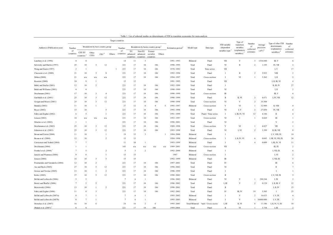
CEE EU

countries a

OtherCEEs FSU

b OthersEU

advancedcountries

Non-EUadvancedcountries

Formersocialistcountries

Others

Lansbury et al. (1996) 4 4 14 11 3 1991–1993 Bilateral Panel VII V 3 1536.840 III, V 6

Selowsky and Martin (1997) 25 10 3 12 221 17 18 1990–1995 Total Panel VI II 2 1.195 IV, VII 3

Wang and Swain (1997) 2 1 1 221 17 18 1978–1992 Total Time series VII I, V 17

Claessens et al. (2000) 21 10 3 8 221 17 18 1992–1996 Total Panel I II 2 3.922 VIII 2

Döhrn (2000) 21 n/a n/a n/a 221 17 18 1994–1997 Total Cross-section I VI 1 3.262 I, II 2

Resmini (2000) 10 9 1 15 15 1991–1995 Total Panel VII I, II, III, VI 4

Babić and Stučka (2001) 12 10 2 221 17 18 1992–1999 Total Panel I II, III, IV 27

Baláž and Williams (2001) 4 4 221 17 18 1990–1999 Total Panel VI I, II 2

Deichmann (2001) 17 10 3 4 221 17 18 1990–1999 Total Cross-section III III, V 4

Garibaldi et al. (2001) 25 10 3 12 221 17 18 1990–1999 Total Panel II II, VI 3 4.671 I, IV, VII 12

Grogan and Moers (2001) 25 10 3 12 221 17 18 1990–1998 Total Cross-section VI V 2 35.508

Bandelj (2002) 11 10 1 27 12 6 4 5 1995–1997 Bilateral Cross-section V VI 1 32.909 II, VIII 4

Beyer (2002) 15 10 5 221 17 18 1995–1998 Total Panel VI I, V 3 27.850 IV, VII 4

Fabry and Zeghni (2002) 6 5 1 221 17 18 1991–1999 Total Panel / Time series I I, III, IV, VI 12 4.186 II 4

Jensen (2002) 18 n/a n/a n/a 221 17 18 1993–1997 Total Cross-section VI I 1 0.669 III 1

Minchev et al. (2002) 1 1 221 17 18 1998–2001 Total Panel VI V 2

Deichmann et al. (2003) 25 10 3 12 221 17 18 1989–1998 Total Cross-section V VI 1 4.827 VII 1

Edmiston et al. (2003) 25 10 3 12 221 17 18 1993–1998 Total Panel VI I, VI 2 3.399 II, III, VII 8

Bevan and Estrin (2004) 11 10 1 19 15 3 1 1994–2000 Bilateral Panel I I, V, VIII, IX 10

Bevan et al. (2004) 12 10 2 15 15 1994–1998 Bilateral Cross-section I I, II, IV, VI 6 0.043 I, III, VI, VII, IX 24

Carstensen and Toubal (2004) 7 7 11 10 1 1993–1999 Bilateral Panel I V 4 0.009 I, III, IV, VI 11

Deichmann (2004) 1 1 143 n/a n/a n/a n/a 1989–2001 Bilateral Cross-section VII III, IX 2

Frenkel et al. (2004) i

7 5 2 5 3 2 1992–2000 Bilateral Panel I I, VII, IX 6

Janicki and Wunnava (2004) 9 8 1 15 15 1997 Bilateral Cross-section I I, VI 2

Jensen (2004) 16 10 3 3 15 15 1992–1999 Bilateral Panel III I, VII, IX 5

Pournarakis and Varsakelis (2004) 12 10 2 221 17 18 1997–2001 Total Panel IV III 6

Ass and Beck (2005) 27 10 5 12 221 17 18 1998–2002 Total Panel VI II 7

Grosse and Trevino (2005) 13 10 1 2 221 17 18 1990–1999 Total Panel I I 1

Kekic (2005) 27 10 5 12 221 17 18 1998–2002 Total Cross-section II I, V, VII, IX 5

Bellak and Leibrecht (2006) 5 5 7 6 1 1996–2002 Bilateral Panel VI V 1 290.244 I, IX 2

Botrić and Škuflić (2006) 7 2 5 221 17 18 1996–2002 Total Panel I, III V 2 0.139 I, II, III, V 12

Brzozowski (2006) 13 10 1 2 221 17 18 1990–2001 Total Panel II I, II, IV 15

Fabry and Zeghni (2006) 11 8 3 221 17 18 1992–2003 Total Panel IV III, IV 19 3.585 I 25

Bellak and Leibrecht (2007a) 8 7 1 7 6 1 1995–2003 Bilateral Panel I V 2 16.633 I, V, IX 6

Bellak and Leibrecht (2007b) 8 7 1 7 6 1 1995–2003 Bilateral Panel I V 1 16800.000 I, V, IX 3

Demekas et al. (2007) 16 10 6 24 16 2 6 1995–2003 Total/Bilateral Panel / Cross-section I, III II, VI 8 11.106 I, II, IV, V, IX 18

Dhakal et al. (2007) j

8 8 221 17 18 186 1995-2004 Total Panel II VI 1 3.758 I, III 2

186

186

186

186

186

186

186

186

186

186

186

186

186

186

186

186

186

186

186

186

186

186

Table 1. List of selected studies on determinants of FDI in transition economies for meta-analysis

Author(s) (Publication year)

Target countries

Estimation period d Model type Data type

FDI variable(dependent

variable) type e

Numberof

collectedestimates

Averageprecision

(AP ) g

Numberof

collectedestimates

Numberof

countries

Breakdown by host country groupNumber

ofcountries

Breakdown by home country group c

Type oftransitionvariables

(explanatory

variables) f

Type of other FDIdeterminants(explanatory

variables) h

1

CEE EU

countries a

OtherCEEs FSU b Others

EUadvancedcountries

Non-EUadvancedcountries

Formersocialistcountries

Others

Bandelj (2008a) 11 10 1 221 17 18 1990–2000 Total Panel IV V 3 9.046 II, VIII 6

Bandelj (2008b) 11 10 1 27 12 6 4 5 1995–1997 Bilateral Cross-section V VI 1 32.963 II, VIII, IX 5

Bellak et al. (2008) 8 7 1 7 6 1 1995–2003 Bilateral Panel I V 4 12.803 I, V, IX 12

Torrisi et al. (2008) 4 4 221 17 18 1989–2006 Total Panel I V 1 0.002 I, III, VIII 3

Bellak and Leibrecht (2009) 8 7 1 7 6 1 1995–2003 Bilateral Panel I V 2 205.808 I, V, IX 6

Bellak et al. (2009) 8 7 1 7 6 1 1995–2004 Bilateral Panel I II, V 9 14.386 I, V, IX 24

Fung et al. (2009) 15 10 5 221 17 18 1990–2004 Total Panel II I, II, III, V, VIII 20

Iwasaki and Suganuma (2009) 21 10 5 6 7 5 2 1990–2005 Total/Bilateral Panel II, IV V 4 4.936 I, II, VIII, IX 24

Leibrecht and Scharler (2009) 7 6 1 7 6 1 1995–2004 Bilateral Panel I V 7 13.131 I, V, IX 20

Mateev (2009) 8 7 1 12 12 2001-2006 Bilateral Panel I I, II, III, IX 24

Merlevede and Schoors (2009) 10 10 12 12 1992–2000 Bilateral Panel III III 1 4.051 I, III, VI, VIII 24

Sova et al. (2009) 4 4 17 13 4 1990-2005 Bilateral Panel II I 1 6.733 I, VI, IX 3

Azam (2010) 3 3 221 17 18 1991–2009 Total Time series II I 3

Bandelj (2010) 10 10 221 17 18 1994–2000 Total Panel IV I, VI 2 2.355 II, VIII 4

Deichmann (2010) j

1 1 156 17 18 26 95 2006 Bilateral Cross-section I III, IV, IX 4

Lefilleur and Maurel (2010) 11 10 1 221 17 18 1993–2005 Total Panel II V 2 29.167 I, IX 10

Michalíková and Galeotti (2010) 1 1 221 17 18 2000–2007 Total Panel VI IV, V, VI 27

Overesch and Wamser (2010) 10 10 1 1996–2005 Bilateral Panel III, VII V, VI 18 7.207 I, III, IV, V 45

Serin and Çalışkan (2010) 9 3 4 2 221 17 18 1995-2006 Total Panel II I, III, VIII 12

Hengel (2011) j

8 2 6 221 17 18 1995-2008 Total Panel III I, III, IV, V, VI 6 3.551 II, III 18

Jiménez (2011) 14 10 4 3 3 1999–2006 Bilateral Panel I I, II 12

Seric (2011) j 10 10 221 17 18 1995-2005 Total Panel III III, V, VI 17 3.155 I, III, V, VII 29

Doytch and Eren (2012) 21 9 5 7 221 17 18 1994–2008 Total Panel VI II, IV, VII 32

Gorbunova et al. (2012) 27 10 5 12 221 17 18 1995–2002 Total Panel III I, II, V, VII, VIII, IX 21

Deichmann (2013) j

1 1 190 17 18 27 128 2000–2009 Bilateral Cross-section III, VII III, IV, IX 6

Derado (2013) 12 10 2 5 4 1 1996–2004 Bilateral Panel III V 3 11.891 I, II, III, VIII, IX 9

Sakali (2013) 1 1 12 10 2 1998–2008 Bilateral Panel I I, VI 1 0.546 I, III, VI, VIII 6

Estrin and Uvalic (2014) j

17 10 6 1 70 17 18 1990-2011 Bilateral Panel I V 4 9.091 I, V, VII, VIII, IX 29

Dauti (2015a) 15 10 5 14 14 1994-2010 Bilateral Panel III I, VI 8 4.315 I, III, IV, VI, IX 19

Dauti (2015b) 15 10 5 20 17 3 1994-2010 Bilateral Panel III I, VI 8 1.083 I, III, IV, VI, IX 16

Igošina (2015) 27 10 17 9 4 2 3 2000-2008 Bilateral Panel I I, II, IV, V, IX 6

Lee (2015) j

20 10 3 7 221 17 18 1995–2006 Total Panel II IV, V, VI 6 3.139 I, III, V 6Notes:a CEE EU countries denote the ten Central and Eastern European countries that joined the European Union either in 2004 or 2007.

b Excluding the Baltic countries.

d The estimation period may differ depending on the target countries within each study.

f I: General transition indicators, II: Liberalization indicators, III: Enterprise reform indicators, IV: Competition policy indicators, V: Privatization indicators, VI: Other indicators (trade and forex systems, efficiency of law institutions, infrastructure reform, financial sector reform, and so on).g AP is defined as the mean of the inverse of the standard errors of estimates collected from each study.

h I: Market size variables, II: Purchasing power variables, III: Trade effect variables, IV: Agglomeration effect variables, V: Labor cost level variables, VI: Labor cost difference variables, VII: Resource abundance variables, VIII: EU accession variables, IX: Geographical distance variables.

i A subpanel with CEE countries is discussed.

j Based on the list of home investment countries in the study, they are divided into four categories according to the country group classificaton of the UNCTAD Handbook of Statistics 2012 (see note c for details).

186

186

186

e I: Annual net FDI inflow, II: Annual gross FDI inflow, III: Cumulative gross FDI value or FDI (including fixed capital) stock, IV: Annual net or gross FDI inflow per capita, V: Cumulative net FDI value per capita, VI: Annual net FDI inflow to GDP (including manufacturing value added) or annual gross FDI inflow to manufacturing output, VII: Others

(number of FDI projects, etc.).

186

186

186

186

186

186

35

186

186

186

186

c For the total FDI model, all home countries are conveniently divided into four categories according to the country group classificaton of the UNCTAD Handbook of Statistics 2012: among 221 countries listed, 17 are classified as EU advanced countries, 18 as non-EU advanced countries, and the remaining 186 as emerging and developing countries,

including the former socialist countries.

Author(s) (Publication year)

Target countries

Estimation period d Model type Data type

Numberof

collectedestimates

Numberof

countries

Breakdown by host country groupNumber

ofcountries

Breakdown by home country group c

FDI variable(dependent

variable) type e

Type oftransitionvariables

(explanatory

variables) f

Numberof

collectedestimates

Averageprecision

(AP ) g

Type of other FDIdeterminants(explanatory

variables) h

Lower class limit Lower class limit

Figure 1. Frequency distribution of partial correlation coefficients

Transition variables (K =185) a

Market size variables (K =210) b

Num

ber

of e

stim

ates

Num

ber

of e

stim

ates

Purchasing power variables (K =90) c

Trade effect variables (K =109) d

Num

ber

of e

stim

ates

Num

ber

of e

stim

ates

Lower class limit Lower class limit

Agglomeration effect variables (K =51) e

Labor cost level variables (K =82) f

Num

ber

of e

stim

ates

Num

ber

of e

stim

ates

Lower class limit Lower class limit

0

10

20

30

40

50

-1.0 -0.8 -0.6 -0.4 -0.2 0.0 0.2 0.4 0.6 0.8 1.0

Mean: 0.186Median: 0.145S.D.: 0.221Max: 0.944Min: -0.457Kurtosis: 4.778Skewness: 0.873

0

4

8

12

16

20

-1.0 -0.8 -0.6 -0.4 -0.2 0.0 0.2 0.4 0.6 0.8 1.0

Mean: 0.024Median: 0.015S.D.: 0.297Max: 0.657Min: -0.746Kurtosis: 2.611Skewness: -0.055

0

4

8

12

16

20

-1.0 -0.8 -0.6 -0.4 -0.2 0.0 0.2 0.4 0.6 0.8 1.0

Mean: 0.402Median: 0.390S.D.: 0.243Max: 0.861Min: 0.070Kurtosis: 1.882Skewness: 0.321

0

5

10

15

20

25

-1.0 -0.8 -0.6 -0.4 -0.2 0.0 0.2 0.4 0.6 0.8 1.0

Mean: -0.039Median: -0.067S.D.: 0.243Max: 0.965Min: -0.632Kurtosis: 5.783Skewness: 1.005

0

10

20

30

40

50

-1.0 -0.8 -0.6 -0.4 -0.2 0.0 0.2 0.4 0.6 0.8 1.0

Mean: 0.293Median: 0.283S.D.: 0.288Max: 0.999Min: -0.456Kurtosis: 3.169Skewness: 0.420

0

5

10

15

20

25

-1.0 -0.8 -0.6 -0.4 -0.2 0.0 0.2 0.4 0.6 0.8 1.0

Mean: 0.186Median: 0.185S.D.: 0.201Max: 0.823Min: -0.441Kurtosis: 3.581Skewness: 0.300

Notes:a Goodness-of-fit test : χ

2=23.80, p =0.000

b Goodness-of-fit test: χ

2=6.39, p =0.041

c Goodness-of-fit test: χ

2=0.48, p =0.788

d Goodness-of-fit test: χ

2=3.80, p =0.150

e Goodness-of-fit test : χ

2=8.47, p =0.015

f Goodness-of-fit test: χ

2=17.28, p =0.000

g Goodness-of-fit test: χ

2=0.10, p =0.953

h Goodness-of-fit test: χ

2=3.89, p =0.143

i Goodness-of-fit test: χ

2=23.32, p =0.000

j Goodness-of-fit test: χ

2=2.59, p =0.274

Labor cost difference variables (K =38) g

Resource abundance variables (K =43) h

Num

ber

of e

stim

ates

Num

ber

of e

stim

ates

Lower class limit Lower class limit

EU accession variables (K =49) i

Geographical distance variables (K =76) j

Num

ber

of e

stim

ates

Num

ber

of e

stim

ates

Lower class limit Lower class limit

0

4

8

12

16

20

-1.0 -0.8 -0.6 -0.4 -0.2 0.0 0.2 0.4 0.6 0.8 1.0

Mean: -0.004Median: -0.038S.D.: 0.167Max: 0.363Min: -0.432Kurtosis: 2.803Skewness: 0.094

0

2

4

6

8

10

-1.0 -0.8 -0.6 -0.4 -0.2 0.0 0.2 0.4 0.6 0.8 1.0

Mean: 0.056Median: 0.025S.D.: 0.277Max: 0.796Min: -0.561Kurtosis: 3.401Skewness: 0.565

0

5

10

15

20

25

-1.0 -0.8 -0.6 -0.4 -0.2 0.0 0.2 0.4 0.6 0.8 1.0

Mean: 0.157Median: 0.134S.D.: 0.158Max: 0.796Min: -0.279Kurtosis: 9.115Skewness: 1.651

0

5

10

15

20

25

-1.0 -0.8 -0.6 -0.4 -0.2 0.0 0.2 0.4 0.6 0.8 1.0

Mean: -0.228Median: -0.243S.D.: 0.187Max: 0.202Min: -0.839Kurtosis: 3.521Skewness: -0.268

Lower class limit Lower class limit

Figure 2. Frequency distribution of t values

Transition variables (K =185) a

Market size variables (K =210) b

Num

ber

of e

stim

ates

Num

ber

of e

stim

ates

Purchasing power variables (K =90) c

Trade effect variables (K =109) d

Num

ber

of e

stim

ates

Num

ber

of e

stim

ates

Lower class limit Lower class limit

Agglomeration effect variables (K =51) e

Labor cost level variables (K =82) f

Num

ber

of e

stim

ates

Num

ber

of e

stim

ates

Lower class limit Lower class limit

0

5

10

15

20

25

-10.0 -7.5 -5.0 -2.5 0.0 2.5 5.0 7.5 10.0

Mean: 2.347Median: 2.300S.D.: 2.348Max: 15.137Min: -3.210Kurtosis: 10.317Skewness: 1.711

0

2

4

6

8

10

-10.0 -7.5 -5.0 -2.5 0.0 2.5 5.0 7.5 10.0

Mean: 0.384Median: 0.129S.D.: 2.578Max: 8.357Min: -4.506Kurtosis: 3.094Skewness: 0.476

0

4

8

12

16

20

-10.0 -7.5 -5.0 -2.5 0.0 2.5 5.0 7.5 10.0

Mean: 2.165Median: 2.206S.D.: 2.139Max: 7.939Min: -1.801Kurtosis: 2.917Skewness: 0.396

0

4

8

12

16

20

-20.0 -15.0 -10.0 -5.0 0.0 5.0 10.0 15.0 20.0

Mean: 5.202Median: 4.346S.D.: 3.314Max: 19.650Min: 1.558Kurtosis: 10.576Skewness: 2.481

0

4

8

12

16

20

-10.0 -7.5 -5.0 -2.5 0.0 2.5 5.0 7.5 10.0

Mean: -0.398Median: -1.667S.D.: 5.876Max: 46.000Min: -6.283Kurtosis: 48.724Skewness: 6.115

0

10

20

30

40

50

60

-20.0 -15.0 -10.0 -5.0 0.0 5.0 10.0 15.0 20.0

Mean: 6.220Median: 3.533S.D.: 11.888Max: 133.522Min: -3.200Kurtosis: 67.061Skewness: 6.969

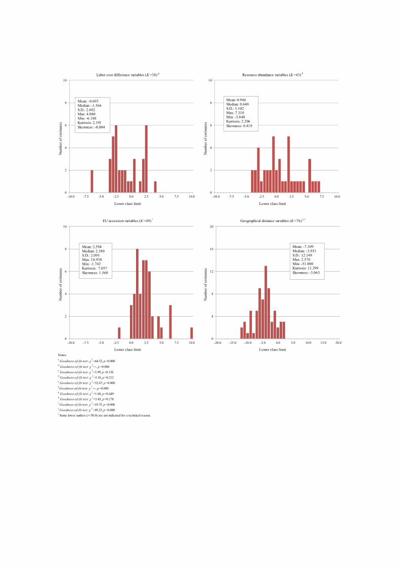
Notes:a Goodness-of-fit test : χ

2=64.52, p =0.000

b Goodness-of-fit test: χ

2=-, p =0.000

c Goodness-of-fit test: χ

2=3.99, p =0.136

d Goodness-of-fit test : χ

2=3.10, p =0.212

e Goodness-of-fit test: χ

2=32.67, p =0.000

f Goodness-of-fit test: χ

2=-, p =0.000

g Goodness-of-fit test : χ

2=1.60, p =0.449

h Goodness-of-fit test: χ

2=3.45, p =0.178

i Goodness-of-fit test: χ

2=19.75, p =0.000

j Goodness-of-fit test : χ

2=49.23, p =0.000

i Some lower outliers (t <50.0) are not indicated for a technical reason.

Labor cost difference variables (K =38) g

Resource abundance variables (K =43) h

Num

ber

of e

stim

ates

Num

ber

of e

stim

ates

Lower class limit Lower class limit

EU accession variables (K =49) i

Geographical distance variables (K =76) j, i

Num

ber

of e

stim

ates

Num

ber

of e

stim

ates

Lower class limit Lower class limit

0

2

4

6

8

10

-10.0 -7.5 -5.0 -2.5 0.0 2.5 5.0 7.5 10.0

Mean: -0.693Median: -1.366S.D.: 2.602Max: 4.080Min: -6.180Kurtosis: 2.191Skewness: -0.004

0

2

4

6

8

10

-10.0 -7.5 -5.0 -2.5 0.0 2.5 5.0 7.5 10.0

Mean: 0.946Median: 0.440S.D.: 3.102Max: 7.310Min: -3.840Kurtosis: 2.206Skewness: 0.419

0

2

4

6

8

10

-10.0 -7.5 -5.0 -2.5 0.0 2.5 5.0 7.5 10.0

Mean: 2.594Median: 2.380S.D.: 2.095Max: 10.930Min: -1.742Kurtosis: 7.057Skewness: 1.560

0

4

8

12

16

20

-20.0 -15.0 -10.0 -5.0 0.0 5.0 10.0 15.0 20.0

Mean: -7.109Median: -3.951S.D.: 12.149Max: 2.576Min: -51.000Kurtosis: 11.399Skewness: -3.063

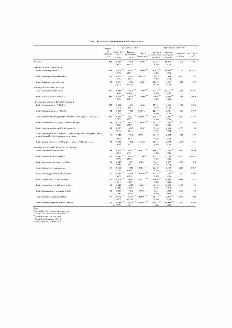
All studies 933 0.006***

0.105***

62000***

60.395***

10.954***

1.977 1256706(20.02) (32.34) (0.00) (0.00)

(a) Comparison in terms of data type

Studies that employ panel data 829 0.006 *** 0.100 *** 60000 *** 57.616 *** 10.554 *** 2.001 1016128(19.49) (29.90) (0.00) (0.00)

Studies that employ cross-sectional data 80 0.075***

0.089***

647.650***

8.679***

1.489*

0.970 2147(8.29) (3.32) (0.00) (0.07)

Studies that employ time series data 24 0.888***

0.756***

68.807**

22.098***

3.539***

4.511 4307(29.77) (12.49) (0.00) (0.00)

(b) Comparison in terms of model type

Studies that adopt total FDI model 487 0.441***

0.229***

14000***

57.664***

12.156***

2.613 597926(116.36) (11.26) (0.00) (0.00)

Studies that adopt bilateral FDI model 446 0.003 *** 0.039 *** 34000 *** 27.097 *** 4.338 *** 1.283 120570(10.67) (12.47) (0.00) (0.00)

(c) Comparison in terms of the type of FDI variable

Studies that use annual net FDI inflow 272 0.084 *** 0.084 *** 46000 *** 27.730 *** 4.608 *** 1.681 77020(48.21) (3.58) (0.00) (0.00)

Studies that use annual gross FDI inflow 152 0.104***

0.138***

2364.112***

22.678***

3.921***

1.839 28737(21.42) (6.91) (0.00) (0.00)

Studies that use cumulative gross FDI value or FDI (including fixed capital) stock 250 0.044***

0.127***

5094.363***

22.678***

3.921***

1.839 28737(27.15) (15.37) (0.00) (0.00)

Studies that use annual net or gross FDI inflow per capita 86 0.204 *** 0.242 *** 265.569 *** 21.331 *** 3.868 *** 2.300 14374(20.53) (12.77) (0.00) (0.00)

Studies that use cumulative net FDI value per capita 13 0.052***

0.047 50.287***

2.434***

0.380 0.675 15(2.74) (1.15) (0.01) (0.35)

Studies that use annual net FDI inflow to GDP (including manufacturing value added)or annual gross FDI inflow to manufacturing output

96 0.322 *** 0.145 *** 2057.314 *** 18.149 *** 3.842 *** 1.852 11589

(34.51) (3.18) (0.00) (0.00)

Studies that use other types of FDI variables (number of FDI projects, etc.) 64 0.001***

0.005***

1131.332***

16.741***

2.372***

2.093 6565(4.54) (2.72) (0.00) (0.01)

(d) Comparison in terms of the type of FDI determinant

Studies that use transition variables 185 0.004***

0.063***

1969.312***

31.924***

5.586***

2.347 69489(8.01) (18.85) (0.00) (0.00)

Studies that use market size variables 210 0.030***

0.279***

35000***

90.137***

15.288***

6.220 630297(47.57) (27.58) (0.00) (0.00)

Studies that use purchasing power variables 90 0.042***

0.035 585.821***

3.639***

0.817 0.384 350(4.36) (1.32) (0.00) (0.21)

Studies that use trade effect variables 109 0.001 0.066 *** 1002.347 *** 22.602 *** 5.540 *** 2.165 20467(1.58) (14.09) (0.00) (0.00)

Studies that use agglomeration effect variables 51 0.123***

0.368***

1098.199***

37.151***

7.333***

5.202 25962(28.83) (15.28) (0.00) (0.00)

Studies that use labor cost level variables 82 -0.003***

-0.015**

2787.725***

-3.603***

-0.580 -0.398 311(-4.64) (-2.28) (0.00) (0.28)

Studies that use labor cost difference variables 38 -0.041 *** -0.022 225.475 *** -4.274 *** -0.965 -0.693 219(-6.58) (-1.29) (0.00) (0.17)

Studies that use resource abundance variables 43 0.058***

0.043**

317.431***

6.205***

1.047 0.946 569(11.19) (2.09) (0.00) (0.15)

Studies that use EU accession variables 49 0.092***

0.140***

214.061***

18.156***

2.977***

2.594 5920(18.07) (10.26) (0.00) (0.00)

Studies that use geographical distance variables 76 -0.381 *** -0.229 *** 3359.708 *** -61.972 *** -10.099 *** -7.109 107786(-107.47) (-9.15) (0.00) (0.00)

Notes:a Null hypothesis: The synthesized effect size is zero.

b Null hypothesis: Effect sizes are homogeneous.

*** Statistical significance at the 1% level

** Statistical significance at the 5% level

* Statistical significance at the 10% level

Median oft values

Fail-safe N(fsN )

Table 2. Synthesis of collected estimates of all FDI determinants

Numberof

estimates(K )

(a) Synthesis of PCCs (b) Combination of t values

Fixed-effectmodel

(z value) a

Random-effects model

(z value) a

Test of

homogeneity b

Unweightedcombination

(p value)

Weightedcombination

(p value)

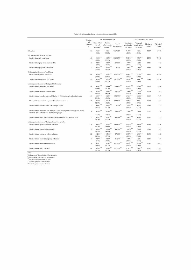
All studies 185 0.004***

0.063***

1969.312***

31.924***

5.586***

2.347 69489(8.01) (18.85) (0.00) (0.00)

(a) Comparison in terms of data type

Studies that employ panel data 165 0.004 *** 0.058 *** 1808.133 *** 30.036 *** 5.307 *** 2.338 54843(7.82) (17.55) (0.00) (0.00)

Studies that employ cross-sectional data 17 0.148***

0.159***

25.080*

7.777***

1.228 1.886 363(6.99) (5.70) (0.00) (0.11)

Studies that employ time series data 3 0.926***

0.926***

0.028 9.431***

1.886**

5.445 96(9.50) (9.50) (0.00) (0.03)

(b) Comparison in terms of model type

Studies that adopt total FDI model 96 0.240***

0.274***

677.378***

24.835***

5.018***

2.535 21785(24.86) (10.04) (0.00) (0.00)

Studies that adopt bilateral FDI model 89 0.003 *** 0.025 *** 691.200 *** 20.233 *** 3.141 *** 2.145 13376(6.84) (10.22) (0.00) (0.00)

(c) Comparison in terms of the type of FDI variable

Studies that use annual net FDI inflow 49 0.068 *** 0.160 *** 294.821 *** 18.048 *** 2.784 *** 2.578 5849(13.08) (9.76) (0.00) (0.00)

Studies that use annual gross FDI inflow 24 0.098***

0.109***

75.306***

8.409***

1.363*

1.716 603(8.91) (4.90) (0.00) (0.09)

Studies that use cumulative gross FDI value or FDI (including fixed capital) stock 55 0.037***

0.155***

854.353***

19.617***

4.904***

2.645 7767(10.48) (9.53) (0.00) (0.00)

Studies that use annual net or gross FDI inflow per capita 29 0.232 *** 0.260 *** 119.629 *** 12.431 *** 2.416 *** 2.308 1627(12.19) (6.28) (0.00) (0.01)

Studies that use cumulative net FDI value per capita 3 0.137***

0.174***

5.209*

3.784***

0.617 2.185 13(3.17) (2.19) (0.00) (0.27)

Studies that use annual net FDI inflow to GDP (including manufacturing value added)or annual gross FDI inflow to manufacturing output

10 0.258 *** 0.288 *** 38.856 *** 7.961 *** 1.134 2.517 224

(7.79) (3.94) (0.00) (0.13)

Studies that use other types of FDI variables (number of FDI projects, etc.) 15 0.002***

0.002**

43.014***

5.812***

0.788 1.501 172(4.74) (2.53) (0.00) (0.22)

(d) Comparison in terms of the type of transition variable

Studies that use general transition indicators 20 0.122***

0.224***

445.870***

18.776***

4.800***

4.198 2586(16.79) (5.66) (0.00) (0.00)

Studies that use liberalization indicators 12 0.205 *** 0.250 *** 48.773 *** 9.676 *** 1.233 2.793 403(8.71) (4.88) (0.00) (0.11)

Studies that use enterprise reform indicators 22 0.260***

0.312***

57.664***

12.373***

2.969***

2.638 1223(11.76) (7.74) (0.00) (0.00)

Studies that use competition policy indicators 17 0.177***

0.159***

71.295***

5.702***

1.251 1.383 187(6.41) (2.61) (0.00) (0.11)

Studies that use privatization indicators 70 0.001 0.048***

591.306***

19.131***

2.909***

2.287 9397(1.63) (11.33) (0.00) (0.00)

Studies that use other indicators 44 0.005***

0.009***

222.536***

11.325***

2.137**

1.707 2041(7.51) (2.72) (0.00) (0.02)

Notes:a Null hypothesis: The synthesized effect size is zero.

b Null hypothesis: Effect sizes are homogeneous.

*** Statistical significance at the 1% level

** Statistical significance at the 5% level

* Statistical significance at the 10% level

Median oft values

Fail-safe N(fsN )

Table 3. Synthesis of collected estimates of transition variables

Numberof

estimates(K )

(a) Synthesis of PCCs (b) Combination of t values

Fixed-effectmodel

(z value) a

Random-effects model

(z value) a

Test of

homogeneity b

Unweightedcombination

(p value)

Weightedcombination

(p value)

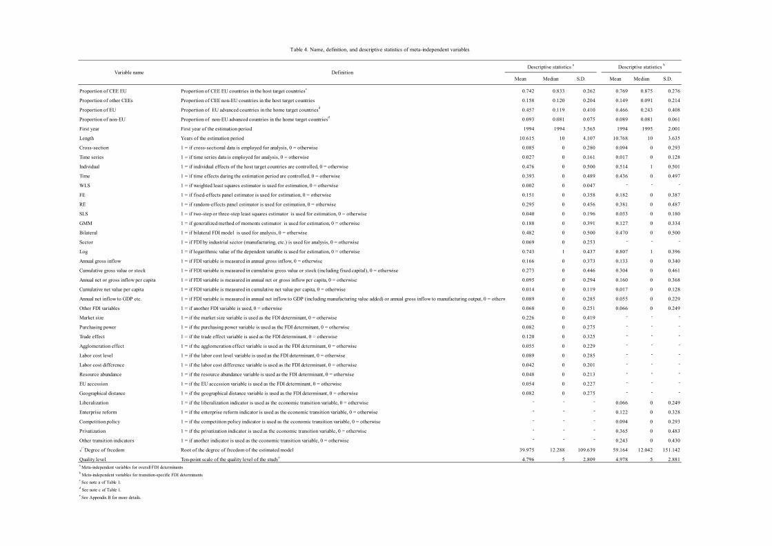
Mean Median S.D. Mean Median S.D.

Proportion of CEE EU Proportion of CEE EU countries in the host target countriesc 0.742 0.833 0.262 0.769 0.875 0.276

Proportion of other CEEs Proportion of CEE non-EU countries in the host target countries 0.158 0.120 0.204 0.149 0.091 0.214

Proportion of EU Proportion of EU advanced countries in the home target countriesd 0.457 0.119 0.410 0.466 0.243 0.408

Proportion of non-EU Proportion of non-EU advanced countries in the home target countriesd 0.093 0.081 0.075 0.089 0.081 0.061

First year First year of the estimation period 1994 1994 3.565 1994 1995 2.001

Length Years of the estimation period 10.615 10 4.107 10.768 10 3.635

Cross-section 1 = if cross-sectional data is employed for analysis, 0 = otherwise 0.085 0 0.280 0.094 0 0.293

Time series 1 = if time series data is employed for analysis, 0 = otherwise 0.027 0 0.161 0.017 0 0.128

Individual 1 = if individual effects of the host target countries are controlled, 0 = otherwise 0.476 0 0.500 0.514 1 0.501

Time 1 = if time effects during the estimation period are controlled, 0 = otherwise 0.393 0 0.489 0.436 0 0.497

WLS 1 = if weighted least squares estimator is used for estimation, 0 = otherwise 0.002 0 0.047 - - -

FE 1 = if fixed-effects panel estimator is used for estimation, 0 = otherwise 0.151 0 0.358 0.182 0 0.387

RE 1 = if random-effects panel estimator is used for estimation, 0 = otherwise 0.295 0 0.456 0.381 0 0.487

SLS 1 = if two-step or three-step least squares estimator is used for estimation, 0 = otherwise 0.040 0 0.196 0.033 0 0.180

GMM 1 = if generalized method of moments estimator is used for estimation, 0 = otherwise 0.188 0 0.391 0.127 0 0.334

Bilateral 1 = if bilateral FDI model is used for analysis, 0 = otherwise 0.482 0 0.500 0.470 0 0.500

Sector 1 = if FDI by industrial sector (manufacturing, etc.) is used for analysis, 0 = otherwise 0.069 0 0.253 - - -

Log 1 = if logarithmic value of the dependent variable is used for estimation, 0 = otherwise 0.743 1 0.437 0.807 1 0.396

Annual gross inflow 1 = if FDI variable is measured in annual gross inflow, 0 = otherwise 0.166 0 0.373 0.133 0 0.340

Cumulative gross value or stock 1 = if FDI variable is measured in cumulative gross value or stock (including fixed capital), 0 = otherwise 0.273 0 0.446 0.304 0 0.461

Annual net or gross inflow per capita 1 = if FDI variable is measured in annual net or gross inflow per capita, 0 = otherwise 0.095 0 0.294 0.160 0 0.368

Cumulative net value per capita 1 = if FDI variable is measured in cumulative net value per capita, 0 = otherwise 0.014 0 0.119 0.017 0 0.128

Annual net inflow to GDP etc. 1 = if FDI variable is measured in annual net inflow to GDP (including manufacturing value added) or annual gross inflow to manufacturing output, 0 = otherw 0.089 0 0.285 0.055 0 0.229

Other FDI variables 1 = if another FDI variable is used, 0 = otherwise 0.068 0 0.251 0.066 0 0.249

Market size 1 = if the market size variable is used as the FDI determinant, 0 = otherwise 0.226 0 0.419 - - -

Purchasing power 1 = if the purchasing power variable is used as the FDI determinant, 0 = otherwise 0.082 0 0.275 - - -

Trade effect 1 = if the trade effect variable is used as the FDI determinant, 0 = otherwise 0.120 0 0.325 - - -

Agglomeration effect 1 = if the agglomeration effect variable is used as the FDI determinant, 0 = otherwise 0.055 0 0.229 - - -

Labor cost level 1 = if the labor cost level variable is used as the FDI determinant, 0 = otherwise 0.089 0 0.285 - - -

Labor cost difference 1 = if the labor cost difference variable is used as the FDI determinant, 0 = otherwise 0.042 0 0.201 - - -

Resource abundance 1 = if the resource abundance variable is used as the FDI determinant, 0 = otherwise 0.048 0 0.213 - - -

EU accession 1 = if the EU accession variable is used as the FDI determinant, 0 = otherwise 0.054 0 0.227 - - -

Geographical distance 1 = if the geographical distance variable is used as the FDI determinant, 0 = otherwise 0.082 0 0.275 - - -

Liberalization 1 = if the liberalization indicator is used as the economic transition variable, 0 = otherwise - - - 0.066 0 0.249

Enterprise reform 1 = if the enterprise reform indicator is used as the economic transition variable, 0 = otherwise - - - 0.122 0 0.328

Competition policy 1 = if the competition policy indicator is used as the economic transition variable, 0 = otherwise - - - 0.094 0 0.293

Privatization 1 = if the privatization indicator is used as the economic transition variable, 0 = otherwise - - - 0.365 0 0.483

Other transition indicators 1 = if another indicator is used as the economic transition variable, 0 = otherwise - - - 0.243 0 0.430

√Degree of freedom Root of the degree of freedom of the estimated model 39.975 12.288 109.639 59.164 12.042 151.142

Quality level Ten-point scale of the quality level of the studye 4.796 5 2.809 4.978 5 2.881a Meta-independent variables for overall FDI determinants

b Meta-independent variables for transition-specific FDI determinants

Table 4. Name, definition, and descriptive statistics of meta-independent variables

e See Appendix B for more details.

Descriptive statistics b

c See note a of Table 1.

d See note c of Table 1.

Variable name DefinitionDescriptive statistics a

(a) Dependent variable — PCC

Estimator (Analytical weightin parentheses)

Meta-independent variable (Default) / Model

Composition of host target countries (FSU countries)

Proportion of CEE EU -0.070 -0.029 -0.004 -0.014 -0.070 -0.068(0.06) (0.06) (0.05) (0.13) (0.06) (0.05)

Proportion of other CEEs 0.140 0.163 * 0.226 ** -0.127 0.129 0.106(0.09) (0.09) (0.10) (0.20) (0.09) (0.07)

Composition of home target countries (Non-advanced countries)

Proportion of EU -0.024 0.038 -0.020 0.063 -0.033 -0.070(0.05) (0.05) (0.05) (0.12) (0.05) (0.05)

Proportion of non-EU -0.029 0.034 -0.066 0.149 -0.038 -0.059(0.15) (0.12) (0.09) (0.24) (0.15) (0.15)

Estimation period

First year -0.012***

-0.009**

-0.016***

0.009 -0.011**

-0.009**

(0.00) (0.00) (0.00) (0.01) (0.00) (0.00)

Length -0.009 ** -0.006 * -0.013 *** 0.014 -0.009 ** -0.009 **

(0.00) (0.00) (0.00) (0.01) (0.00) (0.00)

Data type (Panel data)

Cross-section -0.016 -0.013 -0.022 0.023 -0.041 -0.085*

(0.04) (0.04) (0.03) (0.08) (0.04) (0.04)

Time series 0.231 *** 0.256 *** 0.279 *** 0.238 * 0.237 *** 0.246 ***

(0.06) (0.06) (0.09) (0.13) (0.06) (0.06)

Control for individual and time effects (No control)

Individual -0.027 -0.011 -0.023 -0.029 -0.023 -0.017(0.02) (0.02) (0.02) (0.05) (0.02) (0.03)

Time 0.074***

0.045 0.019 0.065 0.072***

0.074**

(0.03) (0.03) (0.02) (0.05) (0.03) (0.04)

Estimator (OLS)

WLS 0.209***

0.167***

0.215***

0.406***

0.219***

0.235***

(0.06) (0.05) (0.03) (0.11) (0.06) (0.07)

FE -0.042 -0.044 -0.032 -0.189***

-0.051*

-0.064**

(0.03) (0.03) (0.03) (0.05) (0.03) (0.03)

RE -0.024 -0.010 -0.010 -0.080 -0.034 -0.050 **

(0.02) (0.03) (0.02) (0.05) (0.02) (0.02)

SLS -0.020 0.022 0.015 0.039 -0.028 -0.039 *

(0.03) (0.04) (0.03) (0.06) (0.03) (0.02)

GMM -0.064**

-0.081***

-0.063**

-0.015 -0.066**

-0.060**

(0.03) (0.03) (0.03) (0.05) (0.03) (0.02)

Model type (Total FDI model)

Bilateral -0.092 ** -0.113 *** -0.066 ** -0.225 ** -0.081 ** -0.053(0.04) (0.03) (0.03) (0.09) (0.04) (0.04)

Object of FDI (Whole economy)

Sector 0.050 0.048 0.047 -0.117 0.057 0.069*

(0.04) (0.03) (0.04) (0.09) (0.04) (0.04)

Form of dependent variable (Exact numeric value)

Log 0.038 0.037 0.045*

-0.550 0.034 0.023(0.03) (0.03) (0.02) (0.58) (0.03) (0.04)

Type of FDI variable (Annual net inflow)

Annual gross inflow -0.052*

-0.038 -0.012 0.009 -0.051 -0.049(0.03) (0.02) (0.02) (0.06) (0.03) (0.04)

Cumulative gross value or stock -0.011 -0.011 -0.032 -0.039 -0.011 -0.008(0.03) (0.03) (0.02) (0.07) (0.03) (0.03)

Annual net or gross inflow per capita 0.001 0.007 0.013 0.017 -0.014 -0.034(0.04) (0.03) (0.02) (0.07) (0.04) (0.04)

Cumulative net value per capita -0.042 0.003 -0.028 0.250*

-0.026 -0.001(0.07) (0.06) (0.04) (0.13) (0.07) (0.07)

Annual net inflow to GDP etc. 0.005 0.066 0.037 -0.034 0.000 -0.016(0.05) (0.05) (0.05) (0.08) (0.06) (0.07)

Other FDI variables -0.025 -0.002 -0.044 -0.001 -0.026 -0.012(0.04) (0.04) (0.10) (0.15) (0.04) (0.05)

Type of FDI determinant (Transition variables)

Market size 0.094 *** 0.114 *** 0.011 0.050 0.094 *** 0.099 ***

(0.02) (0.03) (0.01) (0.05) (0.02) (0.02)

Purchasing power -0.151 *** -0.174 *** -0.150 *** -0.289 *** -0.151 *** -0.146 ***

(0.04) (0.04) (0.05) (0.07) (0.04) (0.04)

Trade effect 0.006 0.013 -0.002 ** -0.007 0.007 0.011

(0.04) (0.03) (0.00) (0.05) (0.04) (0.04)

Agglomeration effect 0.199***

0.236***

0.090***

0.161**

0.206***

0.215***

(0.06) (0.08) (0.03) (0.07) (0.06) (0.06)

Labor cost level -0.225***

-0.219***

-0.008***

-0.179**

-0.220***

-0.212***

(0.06) (0.06) (0.00) (0.07) (0.06) (0.06)

Labor cost difference -0.143**

-0.080 -0.151***

-0.272***

-0.140**

-0.133**

(0.05) (0.06) (0.03) (0.07) (0.05) (0.06)

Resource abundance -0.173 *** -0.161 *** -0.084 *** -0.184 *** -0.180 *** -0.191 ***

(0.06) (0.05) (0.02) (0.05) (0.06) (0.06)

EU accession 0.004 -0.001 -0.041 -0.074 0.000 -0.010(0.03) (0.02) (0.02) (0.05) (0.03) (0.03)

Geographical distance -0.390***

-0.406***

-0.495***

-0.405***

-0.393***

-0.397***

(0.05) (0.05) (0.11) (0.06) (0.05) (0.05)

Degree of freedom and research quality

√Degree of freedom 0.000 0.000 * 0.000 0.000 0.000 0.000(0.00) (0.00) (0.00) (0.00) (0.00) (0.00)

Quality level -0.005 - -0.008 *** -0.007 -0.005 -0.005(0.00) (-) (0.00) (0.01) (0.00) (0.00)

Intercept 23.586***

17.215**

32.752***

-17.905 22.387***

19.070**

(8.71) (7.13) (6.38) (26.01) (8.59) (9.34)

K 896 896 896 896 896 896

R 2 0.465 0.522 0.542 0.536 - 0.451(continued)

Table 5. Meta-regression analysis of heterogeneity among studies for overall FDI determinants

Cluster-robustOLS

Cluster-robustWLS

[Quality level]

Cluster-robustWLS[N ]

Cluster-robustWLS[1/SE]

Multi-levelmixed effects

RML

Cluster-robustrandom-effects

panel GLS

[1] [2] [3] [4] a [5] [6] b

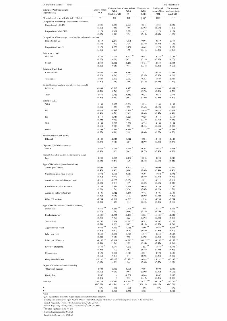
(b) Dependent variable — t value Table 5 (continued)

Estimator (Analytical weightin parentheses)

Meta-independent variable (Default) / Model

Composition of host target countries (FSU countries)

Proportion of CEE EU -1.031 0.027 -2.994 -0.113 -1.031 -1.031(1.17) (1.68) (3.96) (2.06) (1.14) (1.17)

Proportion of other CEEs 1.274 1.828 2.521 -2.437 1.274 1.274(1.65) (2.10) (3.95) (3.14) (1.62) (1.65)

Composition of home target countries (Non-advanced countries)

Proportion of EU 0.559 2.299 4.695 0.804 0.559 0.559(1.06) (1.43) (3.34) (2.56) (1.04) (1.06)

Proportion of non-EU 1.578 4.725 5.430 -0.463 1.578 1.578(3.13) (4.23) (5.98) (5.15) (3.07) (3.13)

Estimation period

First year -0.144*

-0.103 -0.422**

0.181 -0.144**

-0.144*

(0.07) (0.08) (0.21) (0.21) (0.07) (0.07)

Length -0.055 0.000 -0.171 0.464 *** -0.055 -0.055(0.07) (0.08) (0.17) (0.16) (0.07) (0.07)

Data type (Panel data)

Cross-section -0.454 -0.349 0.185 2.135 -0.454 -0.454(0.66) (0.74) (1.37) (2.97) (0.65) (0.66)

Time series -1.087 0.250 -2.762 -0.763 -1.087 -1.087(1.30) (1.46) (3.96) (2.18) (1.28) (1.30)

Control for individual and time effects (No control)

Individual -1.009 ** -0.515 0.423 -0.968 -1.009 *** -1.009 ***

(0.39) (0.36) (0.99) (0.71) (0.38) (0.39)

Time 0.634 0.322 -0.583 -0.127 0.634 0.634(0.42) (0.49) (0.63) (0.95) (0.41) (0.42)

Estimator (OLS)

WLS 1.103 0.377 -2.304 5.154 1.103 1.103(1.17) (1.55) (2.95) (3.61) (1.15) (1.17)

FE -0.923 * -1.443 ** -3.890 * -3.659 *** -0.923 * -0.923 *

(0.48) (0.70) (2.02) (1.00) (0.47) (0.48)

RE 0.113 0.347 1.221 -0.928 0.113 0.113(0.38) (0.45) (0.83) (0.89) (0.37) (0.38)

SLS 0.184 0.703 3.228 0.334 0.184 0.184(0.58) (0.86) (2.05) (1.45) (0.57) (0.58)

GMM -1.599 ** -2.545 ** -6.130 ** -1.538 *** -1.599 ** -1.599 **

(0.73) (0.98) (2.98) (1.03) (0.72) (0.73)

Model type (Total FDI model)

Bilateral -0.148 -1.023 1.622 -0.784 -0.148 -0.148(0.84) (0.75) (2.54) (1.99) (0.83) (0.84)

Object of FDI (Whole economy)

Sector 2.028 ** 2.129 * 8.758 * -0.298 2.028 ** 2.028 **

(0.92) (1.13) (4.65) (1.72) (0.90) (0.92)

Form of dependent variable (Exact numeric value)

Log 0.248 0.355 2.102*

-0.018 0.248 0.248(0.55) (0.54) (1.20) (1.41) (0.54) (0.55)

Type of FDI variable (Annual net inflow)

Annual gross inflow -0.600 -0.583 0.103 -2.512 -0.600 -0.600(0.45) (0.43) (0.80) (2.03) (0.44) (0.45)

Cumulative gross value or stock 1.032 ** 1.118 ** -0.811 -0.797 1.032 *** 1.032 **

(0.40) (0.44) (1.11) (1.60) (0.39) (0.40)

Annual net or gross inflow per capita -0.911 -1.222 -2.636 -2.853 -0.911 * -0.911(0.56) (0.81) (1.79) (2.27) (0.55) (0.56)

Cumulative net value per capita 0.130 0.451 1.446 0.656 0.130 0.130(1.28) (1.36) (3.34) (3.67) (1.26) (1.28)

Annual net inflow to GDP etc. -0.106 0.322 -1.149 -0.473 -0.106 -0.106(0.82) (0.76) (1.75) (1.96) (0.81) (0.82)

Other FDI variables -0.734 -1.361 -4.263 -1.150 -0.734 -0.734(0.87) (1.25) (4.44) (2.38) (0.85) (0.87)

Type of FDI determinant (Transition variables)

Market size 3.255***

4.221***

2.895***

3.686 3.255***

3.255***

(1.20) (1.76) (0.46) (2.21) (1.18) (1.20)

Purchasing power -1.421 *** -1.393 *** -5.201 ** -2.833 *** -1.421 *** -1.421 ***

(0.37) (0.43) (2.22) (0.96) (0.36) (0.37)

Trade effect -0.207 0.024 -1.685 *** 0.285 -0.207 -0.207(0.54) (0.65) (0.09) (1.10) (0.53) (0.54)

Agglomeration effect 3.064 *** 4.312 *** 4.939 *** 2.906 ** 3.064 *** 3.064 ***

(0.97) (0.95) (0.59) (1.40) (0.95) (0.97)

Labor cost level -3.635***

-4.080***

-3.675***

-3.747***

-3.635***

-3.635***

(0.81) (0.98) (0.05) (0.92) (0.80) (0.81)

Labor cost difference -3.157 *** -2.018 * -6.385 *** -6.017 *** -3.157 *** -3.157 ***

(0.84) (1.04) (1.22) (0.94) (0.82) (0.84)

Resource abundance -1.866 ** -1.199 -4.273 -3.553 ** -1.866 ** -1.866 **

(0.85) (1.03) (2.65) (1.42) (0.83) (0.85)

EU accession 0.598 0.811 -3.011 -0.151 0.598 0.598(0.50) (0.51) (2.44) (1.02) (0.49) (0.50)

Geographical distance -10.282***

-12.127**

-35.871**

-10.199**

-10.282***

-10.282***

(3.62) (4.95) (15.44) (3.89) (3.55) (3.62)

Degree of freedom and research quality

√Degree of freedom 0.000 0.000 0.000 -0.004 0.000 0.000(0.00) (0.00) (0.01) (0.00) (0.00) (0.00)

Quality level 0.002 - -0.250 -0.144 0.002 0.002(0.08) (-) (0.15) (0.12) (0.08) (0.08)

Intercept 290.180 * 205.947 848.565 ** -359.257 *** 290.180 ** 290.180 **

(147.08) (158.84) (418.31) (424.21) (144.17) (147.08)

K 896 896 896 896 896 896

R 2 0.300 0.316 0.558 0.383 - 0.300Notes:

Figures in parentheses beneath the regression coefficients are robust standard errors.

b Breusch-Pagan test: χ

2=0.85, p =0.178; Hausman test: χ

2=20.27, p =0.855

c Breusch-Pagan test: χ

2=0.00, p =1.000; Hausman test: χ

2=24.92, p = 0.632

*** Statistical significance at the 1% level

** Statistical significance at the 5% level

* Statistical significance at the 10% level

a Excluding some estimates that report 0.000 or -0.000 as estimated effect sizes, which makes us unable to compute the inverse of the standard error.

Cluster-robustrandom-effects

panel GLS

Cluster-robustOLS

Cluster-robustWLS

[Quality level]

Cluster-robustWLS[N ]

Cluster-robustWLS[1/SE]

Multi-levelmixed effects

RML

[12] c[7] [8] [9] [10] a [11]

(a) Dependent variable — PCC

Estimator (Analytical weightin parentheses)

Meta-independent variable (Default) / Model

Composition of host target countries (FSU countries)

Proportion of CEE EU -0.039 -0.102 0.052 -0.261** -0.023 -0.017

(0.09) (0.12) (0.10) (0.12) (0.05) (0.05)

Proportion of other CEEs 0.167 0.071 0.337 0.056 0.187 *** 0.197 ***

(0.11) (0.14) (0.21) (0.15) (0.06) (0.05)

Composition of home target countries (Non-advanced countries)

Proportion of EU -0.025 -0.081 -0.054 -0.152 0.065 0.054(0.13) (0.12) (0.16) (0.16) (0.12) (0.13)

Proportion of non-EU -0.719 * -0.757 ** -0.450 * -0.151 -0.621 * -0.624 *

(0.42) (0.29) (0.25) (0.23) (0.35) (0.38)

Estimation period

First year 0.000 0.000 -0.015 0.007 -0.010 -0.011(0.01) (0.01) (0.01) (0.01) (0.01) (0.01)

Length 0.007 0.008 -0.023 * -0.006 0.007 0.007(0.01) (0.01) (0.01) (0.01) (0.01) (0.01)

Data type (Panel data)

Cross-section -0.162 ** -0.127 ** -0.204 *** -0.005 -0.188 *** -0.195 **

(0.07) (0.05) (0.05) (0.07) (0.07) (0.08)

Time series 0.652 *** 0.649 *** 0.653 *** 0.502 *** 0.691 *** 0.702 ***

(0.08) (0.11) (0.10) (0.11) (0.05) (0.05)

Control for individual and time effects (No control)

Individual -0.066 * -0.044 -0.053 -0.040 -0.056 -0.052(0.04) (0.03) (0.03) (0.03) (0.04) (0.04)

Time 0.131 ** 0.121 ** 0.053 0.156 *** 0.094 * 0.082(0.05) (0.05) (0.04) (0.05) (0.05) (0.06)

Estimator (OLS)

FE -0.111 * -0.140 ** -0.057 -0.063 -0.123 ** -0.126 **

(0.06) (0.06) (0.06) (0.06) (0.05) (0.06)

RE -0.114 * -0.100 * -0.092 -0.054 -0.118 ** -0.119 **

(0.06) (0.06) (0.06) (0.06) (0.05) (0.05)

SLS -0.226 ** -0.313 *** -0.088 -0.191 ** -0.199 *** -0.196 ***

(0.08) (0.10) (0.07) (0.09) (0.05) (0.05)

GMM -0.115 -0.059 -0.109 ** -0.008 -0.125 * -0.129 *

(0.07) (0.05) (0.05) (0.08) (0.07) (0.07)

Model type (Total FDI model)

Bilateral -0.113 -0.007 -0.069 -0.025 -0.147 -0.148(0.11) (0.08) (0.11) (0.13) (0.09) (0.10)

Form of dependent variable (Exact numeric value)

Log -0.076 -0.051 0.020 -0.052 -0.032 -0.024(0.08) (0.07) (0.07) (0.07) (0.08) (0.09)

Type of FDI variable (Annual net inflow)

Annual gross inflow -0.167 ** -0.097 ** -0.103 ** -0.089 *** -0.213 *** -0.219 ***

(0.07) (0.04) (0.05) (0.02) (0.06) (0.07)

Cumulative gross value or stock -0.038 0.009 -0.074 -0.006 -0.077 -0.083(0.06) (0.06) (0.06) (0.05) (0.06) (0.07)

Annual net or gross inflow per capita 0.019 0.089 * -0.016 0.080 * -0.083 -0.100(0.06) (0.04) (0.05) (0.04) (0.08) (0.09)

Cumulative net value per capita 0.233 ** 0.188 * -0.030 -0.026 0.201 ** 0.197 *

(0.10) (0.09) (0.11) (0.14) (0.10) (0.11)

Annual net inflow to GDP etc. -0.118 -0.053 -0.138 -0.121 -0.123 -0.122(0.10) (0.09) (0.11) (0.07) (0.10) (0.11)

Other FDI variables 1.836 * 2.171 *** 0.183 1.156 ** 1.853 * 1.849 *

(0.95) (0.57) (0.77) (0.52) (0.95) (1.05)

Type of transition variable (General transition indicators)

Liberalization -0.014 0.061 -0.118 -0.029 -0.047 -0.053(0.09) (0.09) (0.08) (0.08) (0.07) (0.08)

Enterprise reform 0.012 0.096 -0.038 -0.074 -0.078 -0.091(0.09) (0.10) (0.07) (0.08) (0.08) (0.08)

Competition policy -0.158 * -0.118 -0.153 ** -0.214 *** -0.252 *** -0.265 ***

(0.09) (0.09) (0.06) (0.07) (0.09) (0.10)

Privatization -0.005 0.074 -0.087 *** -0.106 * -0.059 -0.069(0.07) (0.07) (0.03) (0.06) (0.05) (0.05)

Other transition indicators -0.038 0.058 -0.082 *** -0.148 ** -0.070 -0.075(0.07) (0.08) (0.03) (0.07) (0.05) (0.05)

Degree of freedom and research quality

√Degree of freedom -0.004 ** -0.004 *** -0.001 -0.002 ** -0.004 ** -0.004 **

(0.00) (0.00) (0.00) (0.00) (0.00) (0.00)

Quality level 0.003 - -0.001 -0.003 -0.002 (-0.00)

(0.01) (-) (0.01) (0.01) (0.01) (0.01)

Intercept 1.431 1.297 30.581 -13.272 20.424 23.469(25.82) (20.83) (27.34) (24.55) (19.07) (20.27)

K 179 179 179 179 179 179

R 2 0.572 0.624 0.714 0.794 - 0.509(continued)

[6] a

Table 6. Meta-regression analysis of heterogeneity among studies for transition-specific FDI determinants

Cluster-robustOLS

Cluster-robustWLS

[Quality level]

Cluster-robustWLS[N ]

Cluster-robustWLS[1/SE]

Multi-levelmixed effects

RML

Cluster-robustrandom-effects

panel GLS

[1] [2] [3] [4] [5]

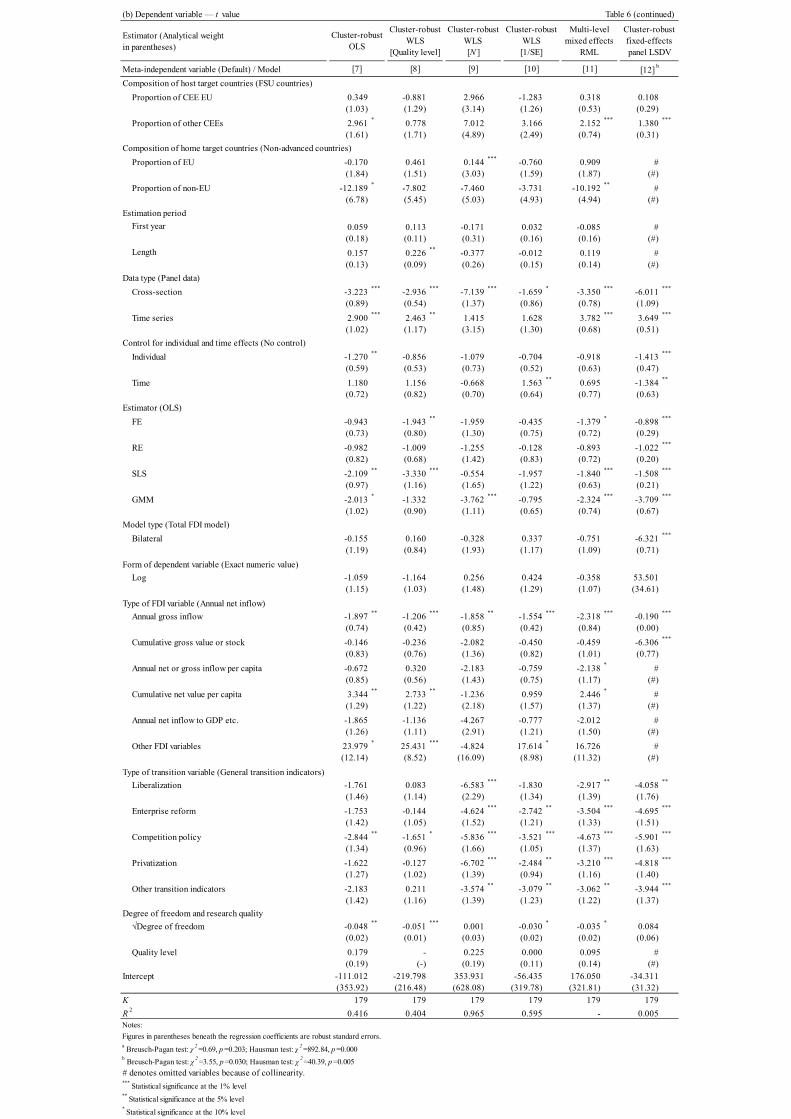
(b) Dependent variable — t value Table 6 (continued)

Estimator (Analytical weightin parentheses)

Meta-independent variable (Default) / Model

Composition of host target countries (FSU countries)

Proportion of CEE EU 0.349 -0.881 2.966 -1.283 0.318 0.108(1.03) (1.29) (3.14) (1.26) (0.53) (0.29)

Proportion of other CEEs 2.961 * 0.778 7.012 3.166 2.152 *** 1.380 ***

(1.61) (1.71) (4.89) (2.49) (0.74) (0.31)

Composition of home target countries (Non-advanced countries)

Proportion of EU -0.170 0.461 0.144 *** -0.760 0.909 #(1.84) (1.51) (3.03) (1.59) (1.87) (#)

Proportion of non-EU -12.189 * -7.802 -7.460 -3.731 -10.192 ** #(6.78) (5.45) (5.03) (4.93) (4.94) (#)

Estimation period

First year 0.059 0.113 -0.171 0.032 -0.085 #(0.18) (0.11) (0.31) (0.16) (0.16) (#)

Length 0.157 0.226 ** -0.377 -0.012 0.119 #(0.13) (0.09) (0.26) (0.15) (0.14) (#)

Data type (Panel data)

Cross-section -3.223 *** -2.936 *** -7.139 *** -1.659 * -3.350 *** -6.011 ***

(0.89) (0.54) (1.37) (0.86) (0.78) (1.09)

Time series 2.900 *** 2.463 ** 1.415 1.628 3.782 *** 3.649 ***

(1.02) (1.17) (3.15) (1.30) (0.68) (0.51)

Control for individual and time effects (No control)

Individual -1.270 ** -0.856 -1.079 -0.704 -0.918 -1.413 ***

(0.59) (0.53) (0.73) (0.52) (0.63) (0.47)

Time 1.180 1.156 -0.668 1.563 ** 0.695 -1.384 **

(0.72) (0.82) (0.70) (0.64) (0.77) (0.63)

Estimator (OLS)

FE -0.943 -1.943 ** -1.959 -0.435 -1.379 * -0.898 ***

(0.73) (0.80) (1.30) (0.75) (0.72) (0.29)

RE -0.982 -1.009 -1.255 -0.128 -0.893 -1.022 ***

(0.82) (0.68) (1.42) (0.83) (0.72) (0.20)

SLS -2.109 ** -3.330 *** -0.554 -1.957 -1.840 *** -1.508 ***

(0.97) (1.16) (1.65) (1.22) (0.63) (0.21)

GMM -2.013 * -1.332 -3.762 *** -0.795 -2.324 *** -3.709 ***

(1.02) (0.90) (1.11) (0.65) (0.74) (0.67)

Model type (Total FDI model)

Bilateral -0.155 0.160 -0.328 0.337 -0.751 -6.321 ***

(1.19) (0.84) (1.93) (1.17) (1.09) (0.71)

Form of dependent variable (Exact numeric value)

Log -1.059 -1.164 0.256 0.424 -0.358 53.501(1.15) (1.03) (1.48) (1.29) (1.07) (34.61)

Type of FDI variable (Annual net inflow)

Annual gross inflow -1.897 ** -1.206 *** -1.858 ** -1.554 *** -2.318 *** -0.190 ***

(0.74) (0.42) (0.85) (0.42) (0.84) (0.00)

Cumulative gross value or stock -0.146 -0.236 -2.082 -0.450 -0.459 -6.306 ***

(0.83) (0.76) (1.36) (0.82) (1.01) (0.77)

Annual net or gross inflow per capita -0.672 0.320 -2.183 -0.759 -2.138 * #(0.85) (0.56) (1.43) (0.75) (1.17) (#)

Cumulative net value per capita 3.344 ** 2.733 ** -1.236 0.959 2.446 * #(1.29) (1.22) (2.18) (1.57) (1.37) (#)

Annual net inflow to GDP etc. -1.865 -1.136 -4.267 -0.777 -2.012 #(1.26) (1.11) (2.91) (1.21) (1.50) (#)

Other FDI variables 23.979 * 25.431 *** -4.824 17.614 * 16.726 #(12.14) (8.52) (16.09) (8.98) (11.32) (#)

Type of transition variable (General transition indicators)

Liberalization -1.761 0.083 -6.583 *** -1.830 -2.917 ** -4.058 **

(1.46) (1.14) (2.29) (1.34) (1.39) (1.76)

Enterprise reform -1.753 -0.144 -4.624 *** -2.742 ** -3.504 *** -4.695 ***

(1.42) (1.05) (1.52) (1.21) (1.33) (1.51)

Competition policy -2.844 ** -1.651 * -5.836 *** -3.521 *** -4.673 *** -5.901 ***

(1.34) (0.96) (1.66) (1.05) (1.37) (1.63)

Privatization -1.622 -0.127 -6.702 *** -2.484 ** -3.210 *** -4.818 ***

(1.27) (1.02) (1.39) (0.94) (1.16) (1.40)

Other transition indicators -2.183 0.211 -3.574 ** -3.079 ** -3.062 ** -3.944 ***

(1.42) (1.16) (1.39) (1.23) (1.22) (1.37)

Degree of freedom and research quality

√Degree of freedom -0.048**

-0.051***

0.001 -0.030*

-0.035*

0.084(0.02) (0.01) (0.03) (0.02) (0.02) (0.06)

Quality level 0.179 - 0.225 0.000 0.095 #(0.19) (-) (0.19) (0.11) (0.14) (#)

Intercept -111.012 -219.798 353.931 -56.435 176.050 -34.311(353.92) (216.48) (628.08) (319.78) (321.81) (31.32)

K 179 179 179 179 179 179

R 2 0.416 0.404 0.965 0.595 - 0.005Notes:

Figures in parentheses beneath the regression coefficients are robust standard errors.a Breusch-Pagan test: χ

2=0.69, p =0.203; Hausman test: χ

2=892.84, p =0.000

b Breusch-Pagan test: χ

2=3.55, p =0.030; Hausman test: χ

2=40.39, p =0.005

# denotes omitted variables because of collinearity.***

Statistical significance at the 1% level**

Statistical significance at the 5% level*

Statistical significance at the 10% level

[12] b

Cluster-robustOLS

Cluster-robustWLS

[Quality level]

Cluster-robustWLS[N ]

Cluster-robustWLS[1/SE]

Multi-levelmixed effects

RML

Cluster-robustfixed-effectspanel LSDV

[7] [8] [9] [10] [11]

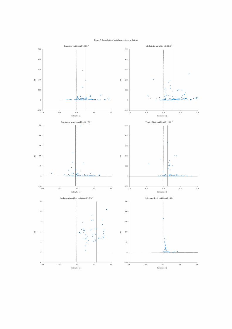
Estimates (r ) Estimates (r )

Figure 3. Funnel plot of partial correlation coefficients

Transition variables (K =181) a

Market size variables (K =204) b

1/SE

1/SE

Purchasing power variables (K =74) c Trade effect variables (K =108) d

1/SE

1/SE

Estimates (r ) Estimates (r )

Agglomeration effect variables (K =50) e

Labor cost level variables (K =80) f

1/SE

1/SE

Estimates (r ) Estimates (r )

-100

0

100

200

300

400

500

-1.0 -0.5 0.0 0.5 1.0-100

0

100

200

300

400

500

-1.0 -0.5 0.0 0.5 1.0

-100

0

100

200

300

400

500

-1.0 -0.5 0.0 0.5 1.0-100

0

100

200

300

400

500

-1.0 -0.5 0.0 0.5 1.0

-100

0

100

200

300

400

500

-1.0 -0.5 0.0 0.5 1.0-6

0

6

12

18

24

30

-1.0 -0.5 0.0 0.5 1.0

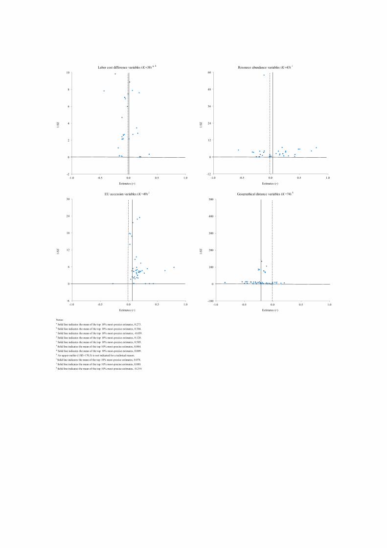
Notes:a Solid line indicates the mean of the top 10% most-precise estimates, 0.273.b Solid line indicates the mean of the top 10% most-precise estimates, 0.304.c Solid line indicates the mean of the top 10% most-precise estimates, -0.059.d Solid line indicates the mean of the top 10% most-precise estimates, 0.120.e Solid line indicates the mean of the top 10% most-precise estimates, 0.589.f Solid line indicates the mean of the top 10% most-precise estimates, 0.004.g Solid line indicates the mean of the top 10% most-precise estimates, 0.009.h An upper outlier (1/SE=170.5) is not indicated for a technical reason.i Solid line indicates the mean of the top 10% most-precise estimates, 0.078.j Solid line indicates the mean of the top 10% most-precise estimates, 0.089.k Solid line indicates the mean of the top 10% most-precise estimates, -0.219.

Labor cost difference variables (K =38) g, h

Resource abundance variables (K =43) i

1/SE

1/SE

Estimates (r ) Estimates (r )

EU accession variables (K =49) j

Geographical distance variables (K =74) k

1/SE

1/SE

Estimates (r ) Estimates (r )

-2

0

2

4

6

8

10

-1.0 -0.5 0.0 0.5 1.0-12

0

12

24

36

48

60

-1.0 -0.5 0.0 0.5 1.0

-100

0

100

200

300

400

500

-1.0 -0.5 0.0 0.5 1.0-6

0

6

12

18

24

30

-1.0 -0.5 0.0 0.5 1.0

1/SE 1/SE

Figure 4. Galbraith plot of t values

Transition variables (K =181) Market size variables (K =204)

Est

imat

es (t

)

Est

imat

es (t

)

Purchasing power variables (K =74) Trade effect variables (K =108)

Est

imat

es (t

)

Est

imat

es (t

)

1/SE 1/SE

Agglomeration effect variables (K =50) Labor cost level variables (K =80)

Est

imat

es (t

)

Est

imat

es (t

)

1/SE 1/SE

-8.0

-6.0

-4.0

-2.0

0.0

2.0

4.0

6.0

8.0

0 100 200 300 400 500-40.0

-30.0

-20.0

-10.0

0.0

10.0

20.0

30.0

40.0

0 100 200 300 400 500

-8.0

-6.0

-4.0

-2.0

0.0

2.0

4.0

6.0

8.0

0 100 200 300 400 500-8.0

-6.0

-4.0

-2.0

0.0

2.0

4.0

6.0

8.0

0 100 200 300 400 500

-10.0

-8.0

-6.0

-4.0

-2.0

0.0

2.0

4.0

6.0

8.0

10.0

0 100 200 300 400 500-20.0

-15.0

-10.0

-5.0

0.0

5.0

10.0

15.0

20.0

0 6 12 18 24 30

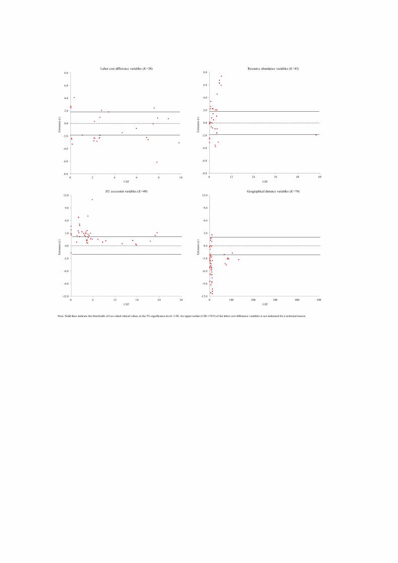
Labor cost difference variables (K =38) Resource abundance variables (K =43)

Est

imat

es (t

)

Est

imat

es (t

)

1/SE 1/SE

Note: Solid lines indicate the thresholds of two-sided critical values at the 5% significance level ±1.96. An upper outlier (1/SE=170.5) of the labor cost difference variables is not indicated for a technical reason.

EU accession variables (K =49) Geographical distance variables (K =74)

Est

imat

es (t

)

Est

imat

es (t

)

1/SE 1/SE

-8.0

-6.0

-4.0

-2.0

0.0

2.0

4.0

6.0

8.0

0 2 4 6 8 10

-8.0

-6.0

-4.0

-2.0

0.0

2.0

4.0

6.0

8.0

0 12 24 36 48 60

-12.0

-9.0

-6.0

-3.0

0.0

3.0

6.0

9.0

12.0

0 100 200 300 400 500-12.0

-9.0

-6.0

-3.0

0.0

3.0

6.0

9.0

12.0

0 6 12 18 24 30

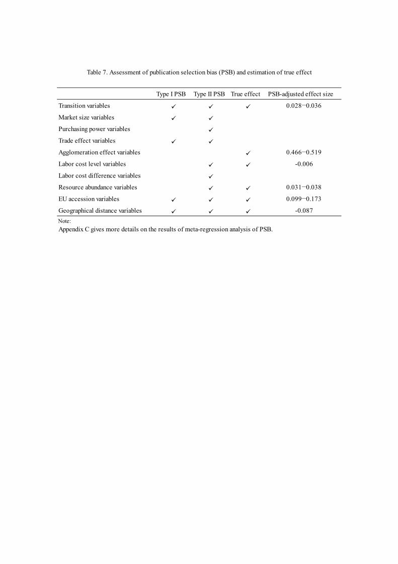
Type I PSB Type II PSB True effect PSB-adjusted effect size

Transition variables 0.028−0.036

Market size variables

Purchasing power variables

Trade effect variables

Agglomeration effect variables 0.466−0.519

Labor cost level variables -0.006

Labor cost difference variables

Resource abundance variables 0.031−0.038

EU accession variables 0.099−0.173

Geographical distance variables -0.087

Note:

Appendix C gives more details on the results of meta-regression analysis of PSB.

Table 7. Assessment of publication selection bias (PSB) and estimation of true effect

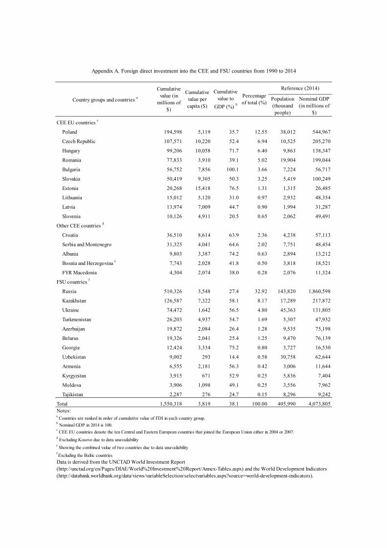
Population(thousandpeople)

Nominal GDP(in millions of

$)

CEE EU countries c

Poland 194,598 5,119 35.7 12.55 38,012 544,967

Czech Republic 107,571 10,220 52.4 6.94 10,525 205,270

Hungary 99,206 10,058 71.7 6.40 9,863 138,347

Romania 77,833 3,910 39.1 5.02 19,904 199,044

Bulgaria 56,752 7,856 100.1 3.66 7,224 56,717

Slovakia 50,419 9,305 50.3 3.25 5,419 100,249

Estonia 20,268 15,418 76.5 1.31 1,315 26,485

Lithuania 15,012 5,120 31.0 0.97 2,932 48,354

Latvia 13,974 7,009 44.7 0.90 1,994 31,287

Slovenia 10,126 4,911 20.5 0.65 2,062 49,491

Other CEE countries d

Croatia 36,510 8,614 63.9 2.36 4,238 57,113

Serbia and Montenegro 31,325 4,041 64.6 2.02 7,751 48,454

Albania 9,803 3,387 74.2 0.63 2,894 13,212

Bosnia and Herzegovina e 7,743 2,028 41.8 0.50 3,818 18,521

FYR Macedonia 4,304 2,074 38.0 0.28 2,076 11,324

FSU countries f

Russia 510,326 3,548 27.4 32.92 143,820 1,860,598

Kazakhstan 126,587 7,322 58.1 8.17 17,289 217,872

Ukraine 74,472 1,642 56.5 4.80 45,363 131,805

Turkmenistan 26,203 4,937 54.7 1.69 5,307 47,932

Azerbaijan 19,872 2,084 26.4 1.28 9,535 75,198

Belarus 19,326 2,041 25.4 1.25 9,470 76,139

Georgia 12,424 3,334 75.2 0.80 3,727 16,530

Uzbekistan 9,002 293 14.4 0.58 30,758 62,644

Armenia 6,555 2,181 56.3 0.42 3,006 11,644

Kyrgyzstan 3,915 671 52.9 0.25 5,836 7,404

Moldova 3,906 1,098 49.1 0.25 3,556 7,962

Tajikistan 2,287 276 24.7 0.15 8,296 9,242

Total 1,550,318 3,819 38.1 100.00 405,990 4,073,805

a Countries are ranked in order of cumulative value of FDI in each country group.

b Nominal GDP in 2014 is 100.

c CEE EU countries denote the ten Central and Eastern European countries that joined the European Union either in 2004 or 2007.

d Excluding Kosovo due to data unavailability

e Showing the combined value of two countries due to data unavailability

f Excluding the Baltic countries

Notes:

Data is derived from the UNCTAD World Investment Report(http://unctad.org/en/Pages/DIAE/World%20Investment%20Report/Annex-Tables.aspx) and the World Development Indicators(http://databank.worldbank.org/data/views/variableSelection/selectvariables.aspx?source=world-development-indicators).

Appendix A. Foreign direct investment into the CEE and FSU countries from 1990 to 2014

Country groups and countries a

Cumulativevalue (in

millions of$)

Cumulativevalue percapita ($)

Cumulativevalue to

GDP (%) b

Percentageof total (%)

Reference (2014)

Appendix B

Method for evaluating the quality level of a study

This appendix describes the evaluation method used to determine the quality level of the studies

subjected to our meta-analysis.

For journal articles, we used the ranking of economics journals that had been published as of

November 1, 2012, by IDEAS—the largest bibliographic database dedicated to economics and

available freely on the Internet (http://ideas.repec.org/)—as the most basic information source for

our evaluation of quality level. IDEAS provides the world’s most comprehensive ranking of

economics journals, and as of November 2012, 1173 academic journals were ranked.

We divided these 1173 journals into 10 clusters using a cluster analysis based on overall

evaluation scores, and assigned each of these journal clusters a score (weight) from 1 (the lowest

journal cluster) to 10 (the highest).

The following table shows a list of 12 academic journals that are representative of the study field

of transition economies along with their IDEAS economics journal ranking [1], their overall scores

[2], and the scores that we assigned in accordance with the above-mentioned procedures [3].

[1] [2] [3]

Journal of Comparative Economics 129 129.98 8 Economics of Transition 138 137.84 8 Emerging Markets Review 162 160.99 7 Economic Systems 230 216.02 7 Economic Change and Restructuring 362 338.54 5 Comparative Economic Studies 397 370.99 5 Emerging Markets Finance and Trade 419 393.71 5 European Journal of Comparative Economics 443 421.53 5 Post-Communist Economies 449 425.82 5 Eastern European Economics 483 456.52 4 Problems of Economic Transition 626 590.06 4 Transition Studies Review 663 625.18 3

For academic journals that are not ranked by IDEAS, we referred to the Thomson Reuters Impact

Factor and other journal rankings and identified the same level of IDEAS ranking-listed journals that

correspond to these non-listed journals; we have assigned each of them the same score as its

counterparts.

Meanwhile, for academic books and book chapters, we have assigned a score of 1 in principle,

but if at least one of the following conditions is met, each of the relevant books or chapters has

uniformly received a score of 4, which is the median value of the scores assigned to the

above-mentioned IDEAS ranking-listed economics journals: (1) The academic book or book chapter

clearly states that it has gone through the peer review process; (2) its publisher is a leading academic

publisher that has external evaluations carried out by experts; or (3) the research level of the study

has been evaluated by the authors to be obviously high.

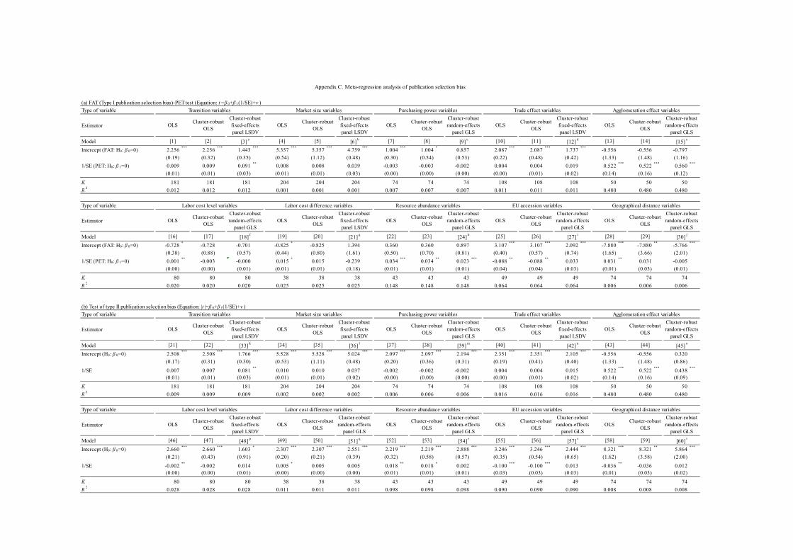
(a) FAT (Type I publication selection bias)-PET test (Equation: t =β 0+β 1(1/SE)+v )

Type of variable

Estimator

Model

Intercept (FAT: H0: β 0=0) 2.256***

2.256***

1.443***

5.357***

5.357***

4.759***

1.004***

1.004*

0.857 2.087***

2.087***

1.737***

-0.556 -0.556 -0.797

(0.19) (0.32) (0.35) (0.54) (1.12) (0.48) (0.30) (0.54) (0.53) (0.22) (0.48) (0.42) (1.33) (1.48) (1.16)

1/SE (PET: H0: β 1=0) 0.009 0.009 0.091**

0.008 0.008 0.039 -0.003 -0.003 -0.002 0.004 0.004 0.019 0.522***

0.522***

0.560***

(0.01) (0.01) (0.03) (0.01) (0.01) (0.03) (0.00) (0.00) (0.00) (0.00) (0.01) (0.02) (0.14) (0.16) (0.12)

K 181 181 181 204 204 204 74 74 74 108 108 108 50 50 50

R2

0.012 0.012 0.012 0.001 0.001 0.001 0.007 0.007 0.007 0.011 0.011 0.011 0.480 0.480 0.480

Type of variable

Estimator

Model

Intercept (FAT: H0: β 0=0) -0.728*

-0.728 -0.701 -0.825*

-0.825 1.394 0.360 0.360 0.897 3.107***

3.107***

2.092***

-7.880***

-7.880**

-5.766***

(0.38) (0.88) (0.57) (0.44) (0.80) (1.61) (0.50) (0.70) (0.81) (0.40) (0.57) (0.74) (1.65) (3.66) (2.01)

1/SE (PET: H0: β 1=0) 0.001**

-0.003 -0.000 0.015*

0.015 -0.239 0.034***

0.034**

0.023***

-0.088**

-0.088**

0.033 0.031**

0.031 -0.005

(0.00) (0.00) (0.01) (0.01) (0.01) (0.18) (0.01) (0.01) (0.01) (0.04) (0.04) (0.03) (0.01) (0.03) (0.01)

K 80 80 80 38 38 38 43 43 43 49 49 49 74 74 74

R2

0.020 0.020 0.020 0.025 0.025 0.025 0.148 0.148 0.148 0.064 0.064 0.064 0.006 0.006 0.006

(b) Test of type II publication selection bias (Equation: |t |=β 0+β 1(1/SE)+v )

Type of variable

Estimator

Model

Intercept (H0: β 0=0) 2.508***

2.508***

1.766***

5.528***

5.528***

5.024***

2.097***

2.097***

2.194***

2.351***

2.351***

2.105***

-0.556 -0.556 0.320

(0.17) (0.31) (0.30) (0.53) (1.11) (0.48) (0.20) (0.36) (0.31) (0.19) (0.41) (0.40) (1.33) (1.48) (0.86)

1/SE 0.007 0.007 0.081**

0.010 0.010 0.037 -0.002 -0.002 -0.002 0.004 0.004 0.015 0.522***

0.522***

0.438***

(0.01) (0.01) (0.03) (0.01) (0.01) (0.02) (0.00) (0.00) (0.00) (0.00) (0.01) (0.02) (0.14) (0.16) (0.09)

K 181 181 181 204 204 204 74 74 74 108 108 108 50 50 50

R2

0.009 0.009 0.009 0.002 0.002 0.002 0.006 0.006 0.006 0.016 0.016 0.016 0.480 0.480 0.480

Type of variable

Estimator

Model

Intercept (H0: β 0=0) 2.660***

2.660***

1.603*

2.307***

2.307***

2.551***

2.219***

2.219***

2.888***

3.246***

3.246***

2.444***

8.321***

8.321**

5.864***

(0.21) (0.43) (0.91) (0.20) (0.21) (0.39) (0.32) (0.58) (0.57) (0.35) (0.54) (0.65) (1.62) (3.58) (2.00)

1/SE -0.002**

-0.002 0.014 0.005*

0.005 0.005 0.018**

0.018*

0.002 -0.100***

-0.100***

0.013 -0.036**

-0.036 0.012(0.00) (0.00) (0.01) (0.00) (0.00) (0.00) (0.01) (0.01) (0.01) (0.03) (0.03) (0.03) (0.01) (0.03) (0.02)

K 80 80 80 38 38 38 43 43 43 49 49 49 74 74 74

R2

0.028 0.028 0.028 0.011 0.011 0.011 0.098 0.098 0.098 0.090 0.090 0.090 0.008 0.008 0.008

OLSCluster-robust

OLSOLS

Cluster-robustOLS

Cluster-robustfixed-effectspanel LSDV

OLSCluster-robust

OLS

Cluster-robustfixed-effectspanel LSDV

Appendix C. Meta-regression analysis of publication selection bias

Transition variables Market size variables Purchasing power variables Trade effect variables Agglomeration effect variables

OLSCluster-robust

OLS

Cluster-robustrandom-effects

panel GLS

Cluster-robustrandom-effects

panel GLSOLS

Cluster-robustOLS

Cluster-robustfixed-effectspanel LSDV

[14] [15] e

Labor cost level variables Labor cost difference variables Resource abundance variables EU accession variables Geographical distance variables

[8] [9] c [10] [11] [12]

d [13][1] [2] [3] a [4] [5] [6]

b [7]

OLSCluster-robust

OLS

Cluster-robustrandom-effects

panel GLS

[16] [17] [18] f [19] [20] [21]

g [22]

OLSCluster-robust

OLS

Cluster-robustrandom-effects

panel GLSOLS

Cluster-robustOLS

Cluster-robustrandom-effects

panel GLSOLS

Cluster-robustOLS

Cluster-robustrandom-effects

panel GLSOLS

Cluster-robustOLS

Cluster-robustfixed-effectspanel LSDV

[29] [30] j

Transition variables Market size variables Purchasing power variables Trade effect variables Agglomeration effect variables

[23] [24] h [25] [26] [27]

i [28]

OLSCluster-robust

OLS

Cluster-robustrandom-effects

panel GLS

[31] [32] [33] k [34] [35] [36]

l [37]

OLSCluster-robust

OLS

Cluster-robustrandom-effects

panel GLSOLS

Cluster-robustOLS

Cluster-robustfixed-effectspanel LSDV

OLSCluster-robust

OLS

Cluster-robustfixed-effectspanel LSDV

OLSCluster-robust

OLS

Cluster-robustfixed-effectspanel LSDV

[44] [45] o

Labor cost level variables Labor cost difference variables Resource abundance variables EU accession variables Geographical distance variables

[38] [39] m [40] [41] [42]

n [43]

OLSCluster-robust

OLS

Cluster-robustrandom-effects

panel GLS

[46] [47] [48] p [49] [50] [51]

q [52]

OLSCluster-robust

OLS

Cluster-robustrandom-effects

panel GLSOLS

Cluster-robustOLS

Cluster-robustrandom-effects

panel GLSOLS

Cluster-robustOLS

Cluster-robustfixed-effectspanel LSDV

OLSCluster-robust

OLS

Cluster-robustrandom-effects

panel GLS

[59] [60] t[53] [54]

r [55] [56] [57] s [58]

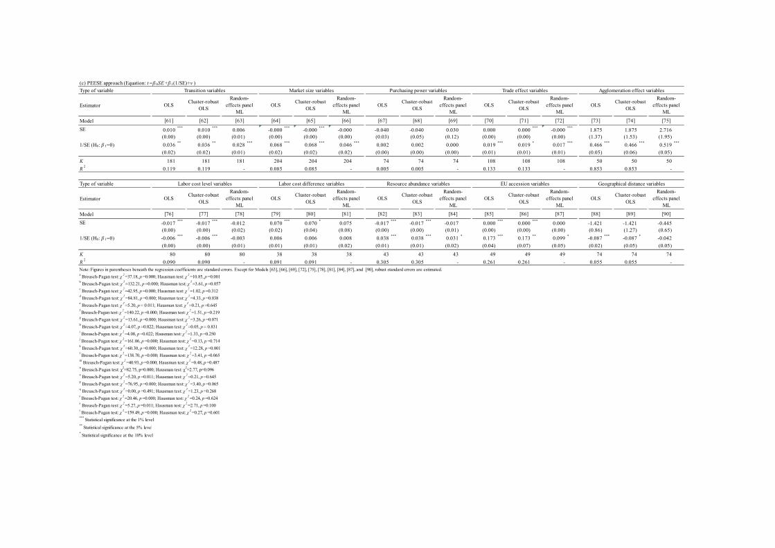
(c) PEESE approach (Equation: t =β 0SE +β 1(1/SE)+v )

Type of variable

Estimator

Model

SE 0.010***

0.010***

0.006 -0.000***

-0.000***

-0.000 -0.040 -0.040 0.030 0.000 0.000***

-0.000***

1.875 1.875 2.716(0.00) (0.00) (0.01) (0.00) (0.00) (0.00) (0.03) (0.05) (0.12) (0.00) (0.00) (0.00) (1.37) (1.53) (1.95)

1/SE (H0: β 1=0) 0.036**

0.036**

0.028***

0.068***

0.068***

0.046***

0.002 0.002 0.000 0.019***

0.019*

0.017***

0.466***

0.466***

0.519***

(0.02) (0.02) (0.01) (0.02) (0.02) (0.02) (0.00) (0.00) (0.00) (0.01) (0.01) (0.01) (0.05) (0.06) (0.05)

K 181 181 181 204 204 204 74 74 74 108 108 108 50 50 50

R2

0.119 0.119 - 0.085 0.085 - 0.005 0.005 - 0.133 0.133 - 0.853 0.853 -

Type of variable

Estimator

Model

SE -0.017***

-0.017***

-0.012 0.070***

0.070*

0.075 -0.017***

-0.017***

-0.017 0.000***

0.000***

0.000 -1.421 -1.421 -0.445(0.00) (0.00) (0.02) (0.02) (0.04) (0.08) (0.00) (0.00) (0.01) (0.00) (0.00) (0.00) (0.86) (1.27) (0.65)

1/SE (H0: β 1=0) -0.006***

-0.006***

-0.003 0.006 0.006 0.008 0.038***

0.038***

0.031*

0.173***

0.173**

0.099*

-0.087***

-0.087*

-0.042

(0.00) (0.00) (0.01) (0.01) (0.01) (0.02) (0.01) (0.01) (0.02) (0.04) (0.07) (0.05) (0.02) (0.05) (0.05)

K 80 80 80 38 38 38 43 43 43 49 49 49 74 74 74

R2

0.090 0.090 - 0.091 0.091 - 0.305 0.305 - 0.261 0.261 - 0.055 0.055 -Note: Figures in parentheses beneath the regression coefficients are standard errors. Except for Models [63], [66], [69], [72], [75], [78], [81], [84], [87], and [90], robust standard errors are estimated.a Breusch-Pagan test: χ

2=37.18, p =0.000; Hausman test: χ

2=10.85, p =0.001

b Breusch-Pagan test: χ

2=132.21, p =0.000; Hausman test: χ

2=3.61, p =0.057

c Breusch-Pagan test: χ

2=42.95, p =0.000; Hausman test: χ

2=1.02, p =0.312

d Breusch-Pagan test: χ

2=84.81, p =0.000; Hausman test: χ

2=4.33, p =0.038

e Breusch-Pagan test: χ

2=5.20, p = 0.011; Hausman test: χ

2=0.21, p =0.645

f Breusch-Pagan test: χ

2=140.22, p =0.000; Hausman test: χ

2=1.51, p =0.219

g Breusch-Pagan test: χ

2=13.61, p =0.000; Hausman test: χ

2=3.26, p =0.071

h Breusch-Pagan test: χ

2=4.07, p =0.022; Hausman test: χ

2=0.05, p = 0.831

i Breusch-Pagan test: χ

2=4.08, p =0.022; Hausman test: χ

2=1.33, p =0.250

j Breusch-Pagan test: χ

2=161.06, p =0.000; Hausman test: χ

2=0.13, p =0.714

k Breusch-Pagan test: χ

2=60.30, p =0.000; Hausman test: χ

2=12.28, p =0.001

l Breusch-Pagan test: χ

2=138.70, p =0.000; Hausman test: χ

2=3.41, p =0.065

m Breusch-Pagan test: χ

2=40.93, p =0.000; Hausman test: χ

2=0.48, p =0.487

n Breusch-Pagan test: χ

2=82.75, p=0.000; Hausman test: χ

2=2.77, p=0.096

o Breusch-Pagan test: χ

2=5.20, p =0.011; Hausman test: χ

2=0.21, p =0.645

p Breusch-Pagan test: χ

2=76.95, p =0.000; Hausman test: χ

2=3.40, p =0.065

q Breusch-Pagan test: χ

2=0.00, p =0.491; Hausman test: χ

2=1.23, p =0.268

r Breusch-Pagan test: χ

2=20.46, p =0.000; Hausman test: χ

2=0.24, p =0.624

s Breusch-Pagan test: χ

2=5.27, p =0.011; Hausman test: χ

2=2.71, p =0.100

t Breusch-Pagan test: χ

2=159.49, p =0.000; Hausman test: χ

2=0.27, p =0.601

*** Statistical significance at the 1% level

** Statistical significance at the 5% level

* Statistical significance at the 10% level

Transition variables Market size variables Purchasing power variables Trade effect variables Agglomeration effect variables

OLSCluster-robust

OLS

Random-effects panel

ML

[61] [62] [63] [64] [65] [66] [67]

OLSCluster-robust

OLS

Random-effects panel

MLOLS

Cluster-robustOLS

Random-effects panel

MLOLS

Cluster-robustOLS

Random-effects panel

MLOLS

Cluster-robustOLS

Random-effects panel

ML

[74] [75]

Labor cost level variables Labor cost difference variables Resource abundance variables EU accession variables Geographical distance variables

[68] [69] [70] [71] [72] [73]

[76] [77] [78] [79] [80] [81] [82]

OLSCluster-robust

OLSOLS

Cluster-robustOLS

Random-effects panel

MLOLS

Cluster-robustOLS

Random-effects panel

ML

[89] [90][83] [84] [85] [86] [87] [88]

OLSCluster-robust

OLS

Random-effects panel

ML

Random-effects panel

MLOLS

Cluster-robustOLS

Random-effects panel

ML