THERMODYNAMICS OF MOLTEN SALTS FOR NUCLEAR APPLICATIONS

Ondřej Beneš

JRC-ITU-TN-2008/40

INSTITUTE OF CHEMICAL TECHNOLOGY, PRAGUE

Faculty of Chemical Technology Department of Inorganic Chemistry

Dissertation

THERMODYNAMICS OF MOLTEN SALTS FOR NUCLEAR APPLICATIONS

Author: Ing. Ondřej Beneš

Supervisor: Prof. Dr. Ing. David Sedmidubský, Dr. Rudy J. M. Konings

Study program: Chemistry

Field of study: Inorganic Chemistry Prague 2008

VYSOKÁ ŠKOLA CHEMICKO-TECHNOLOGICKÁ V PRAZE Fakulta chemické technologie

Ústav Anorganické Chemie

Disertační práce

Termodynamika jaderných paliv na bázi roztavených solí

Autor: Ing. Ondřej Beneš

Školitel: Prof. Dr. Ing. David Sedmidubský, Dr. Rudy J. M. Konings

Studijní program: Chemie

Studijní obor: Anorganická Chemie Praha 2008

Declaration

The thesis was worked out at the Department of Inorganic Chemistry, Institute of Chemical Technology, Prague, from August 2005 to September 2008. „I hereby declare that I have worked out the thesis independently while noting all the resources employed as well as co-authors. I consent to the publication of the thesis under Act No. 111/1998, Coll., on universities, as amended by subsequent regulations.“ Prague, 19.9.2008 .................................................................................................. Signature

Acknowledgement

I want to thank Dr. Rudy J. M. Konings who supervised my thesis at my working place in the Institute for Transuranium Elements (ITU) in Karlsruhe, who was always very willing to help me with whatever task I wanted to discuss. I also want to thank him for very fruitful advices he gave me in the course of my 3 years stay in ITU. I acknowledge my Professor David Sedmidubský who was always very open for discussion on any topic, not only concerning thermodynamics. Dr. Philippe Zeller is thanked for advices and guidance in the field of ab initio calculations.

Furthermore I would like to thank my PhD colleagues, namely Dr. J. P. M. van der Meer and C. Kűnzel from ITU for their help and for their enthusiasm to solve problems together. The technical support staff from the material research unit of ITU is thanked for their significant help, especially concerning the new designs and developments in the lab.

I acknowledge the European Commission for support given in the frame of the program 'Training and Mobility of Researchers' as well as the ACTINET for the fellowship provided in order to temporarly stay in CEA Saclay to perform the ab initio calculations.

Ing. Ondřej Beneš Title: Thermodynamics of the molten salts for nuclear applications Supervisor: Prof. Dr. Ing. David Sedmidubský Study programme: Chemistry Subprogramme: Inorganic Chemistry SUMMARY

The molten salt reactor (MSR) is one of the six reactor concepts of the Generation IV initiative, an international collaboration to study the next generation nuclear power reactors. The fuel of the MSR is based on the dissolution of the fissile material (235U, 233U or 239Pu) in a matrix of a molten salt that must fulfill several requirements with respect to its physical properties. These requirements are very well satisfied by the various systems containing alkali metal and alkali earth fluorides.

In this study in total 32 binary fluoride systems have been thermodynamically assessed in order to predict the fuel properties in terms of the melting behaviour, the vapour pressure and the solubility of the actinides in the fuel matrix. Based on these properties, in total eight fuel compositions for the MSR have been proposed.

As part of the experimental study, two gas tight crucibles have been developped in order to measure the fluoride samples up to high temperatures. One is designed for a drop calorimeter used to measure the heat capacity of the (Li,Na)F liquid solution, whereas the other one is designed for a Differential Scanning Calorimeter (DSC) which was used to determine the equilibrium data points of the NaNO3-KNO3, RbF-CsF and CaF2-ThF4 binary systems. The data of the two latter systems were used to improve our thermodynamic database.

The Schottky contributions of the UPd3 sample were measured by the drop calorimeter and a very good correlation to the theoretical curve has been obtained. This measurement also confirmed that the drop calorimetry is in general a very sensitive method to determine relatively small energies.

An approach of obtaining the excess Gibbs energies of the solutions ab initio has been demonstrated in the case of (Rb,Cs)F solid solution and a very good correlation with the measured solidus and liquidus data has been observed.

Outline: Chapter 1 – Introduction ................................................................................................ 1 Chapter 2 – Nuclear Energy .......................................................................................... 3 2.1 Nuclear Force .................................................................................................. 3 2.2 Nuclear Fission ............................................................................................... 4 Isotopical compositions of the fuels ......................................................... 6 2.3 The Nuclear Fuel Cycle .................................................................................. 7 2.4 Nuclear Reactors ............................................................................................. 7 Current types of nuclear power reactors .................................................... 7 Generation IV reactors .............................................................................. 9 2.5 Molten Salt Reactor ......................................................................................... 11 MSR description ........................................................................................ 11 Advantages of the MSR ............................................................................. 12 Drawbacks of the MSR .............................................................................. 13 History of the MSR .................................................................................... 13 Fuel concepts in the MSR .......................................................................... 14 Other nuclear applications of the molten salts ........................................... 15 Chapter 3 – Thermodynamics ....................................................................................... 18 3.1 Thermodynamic modelling ............................................................................. 19

Thermodynamic models for the excess Gibbs parameters of the binary solutions .................................................................................................... 25

Thermodynamic origin of phase diagrams ............................................... 29 Higher order systems approximation ........................................................ 30 Ternary phase diagrams ............................................................................ 33 Chapter 4 – Thermodynamic Data ............................................................................... 38 4.1 Calorimetry ..................................................................................................... 39 Temperature calibration ............................................................................ 42 Schottky determination in UPd3 ................................................................ 46 High temperature heat capacity ..................................................... 46 The Schottky anomaly in UPd3 ..................................................... 48 Encapsulation technique for the drop mode .............................................. 52 Heat capacity of the (Li,Na)F liquid solution ............................................ 58 4.2 Equilibrium studies ......................................................................................... 63 Temperature calibration ............................................................................. 65 Encapsulation technique for the DSC detector .......................................... 65 Measurement of the NaNO3-KNO3 phase diagram ................................... 69 Measurement of the RbF-CsF phase diagram ............................................ 70 Measurement of the CaF2-ThF4 phase diagram ......................................... 73 4.3 First principle calculations ............................................................................... 78 (Rb,Cs)F solid solution ............................................................................... 78 ab initio calculation .................................................................................... 79 Configurational energy models .................................................................. 80 Calculation of the partition function .......................................................... 83 Bragg-Williams model ................................................................... 84 The quasi-chemical “Guggenheim” model .................................... 85 Thermodynamic assessment of the RbF-CsF phase diagram ..................... 85

Chapter 5 – Binary Systems ............................................................................................ 91 5.1 Fluoride systems .............................................................................................. 92 LiF-NaF system ......................................................................................... 92 LiF-KF system ........................................................................................... 92 LiF-RbF system ......................................................................................... 92 LiF-CsF system .......................................................................................... 94 LiF-BeF2 system ........................................................................................ 97 LiF-LaF3 and NaF-LaF3 systems ............................................................... 97 LiF-ZrF4 system ......................................................................................... 102 LiF-PuF3 system ......................................................................................... 102 NaF-KF system .......................................................................................... 102 NaF-RbF system ......................................................................................... 102 NaF-CsF system ......................................................................................... 109 NaF-BeF2 system ....................................................................................... 111 NaF-PuF3 system ........................................................................................ 112 KF-RbF system ........................................................................................... 113 KF-CsF system ........................................................................................... 114 KF-LaF3 system ......................................................................................... 115 RbF-CsF system ......................................................................................... 117 RbF-LaF3 system ........................................................................................ 117 CsF-LaF3 system ........................................................................................ 117 UF4-ZrF4 system ......................................................................................... 119 BeF2-ZrF4 system ....................................................................................... 121 BeF2-PuF3 and LaF3-PuF3 systems ............................................................. 121 KF-PuF3, RbF-PuF3 and CsF-PuF3 systems ............................................... 123 5.2 Chloride systems .............................................................................................. 129 NaCl-UCl3 system ...................................................................................... 129 NaCl-PuCl3 system ..................................................................................... 129 UCl3-PuCl3 system ..................................................................................... 131 MgCl2-UCl3 system .................................................................................... 131 MgCl2-PuCl3 system ................................................................................... 132 Chapter 6 – Ternary systems .......................................................................................... 134 LiF-NaF-KF phase diagram ........................................................................ 134 LiF-NaF-RbF phase diagram ...................................................................... 135 LiF-NaF-BeF2 phase diagram ..................................................................... 135 LiF-BeF2-PuF3 phase diagram .................................................................... 138 NaF-BeF2-PuF3 phase diagram ................................................................... 140 LiF-NaF-PuF3 phase diagram ..................................................................... 140 LiF-BeF2-ZrF4 phase diagram .................................................................... 148 Chapter 7 – Nuclear Fuel Compositions ........................................................................ 152 7.1 Molten Salt thermal reactor: LiF-BeF2-ZrF4-UF4 system ................................ 153 7.2 Actinide burner non-moderated reactor: LiF-NaF-BeF2-PuF3 system ............. 157 melting behaviour ....................................................................................... 157 vapour pressure ........................................................................................... 160 7.3 Actinide burner non-moderated reactor: LiF-NaF-KF-RbF-(CsF)-PuF3

system .................................................................................................................... 162

melting behaviour ....................................................................................... 162 solubility for actinides ................................................................................ 163 vapour pressure ........................................................................................... 172 influence of the CsF fission product .......................................................... 176 7.4 Molten salt fast breeder fuel: NaCl-MgCl2-UCl3-PuCl3 system ...................... 179 melting behaviour ....................................................................................... 179 vapour pressure ........................................................................................... 180 Chapter 8 – Conclusions and Summary......................................................................... 184 Appendix 1 - The thermodynamic data of all pure compounds considered in this study ........................................................................................................................ 189 Appendix 2 - The excess Gibbs energy data used in this study ........................................ 194 Bibliography ...................................................................................................................... 199

Chapter 1

Introduction

The molten salt reactor (MSR) is one of the six reactor concepts of the Gen-eration IV (GenIV) initiative, an international collaboration to study the nextgeneration nuclear power reactors. The fuel of the MSR is based on the dis-solution of the fissile material (235U, 233U or 239Pu) in a matrix of a moltensalt that must fulfill several requirements with respect to its physical proper-ties. These requirements are very well fulfilled by the various systems containingalkali metal and alkali earth fluorides.

The main task of this study was to extend the thermodynamic database ofthe various systems that are of relevance to the MSR project. The results of thiswork are very important, because once the thermodynamic model is establishedit is possible to predict some of the fuel properties such as melting behaviour,vapour pressure or solubility of actinides in the fuel matrix. Moreover it is mucheasier to optimize the fuel choice by varying the composition with respect to itsproperties.

Basically the thermodynamic modelling consists of two main parts. Firstlyall available experimental data are collected and these are then used to optimizethe phase diagrams in order to obtain the best possible fit between the exper-iment and calculated model. Hence also this study consisted of experimentaland modelling part.

The whole thesis is divided into five main sections. In the first one (Chap-ter 2) the nuclear energy topic is introduced with the scope on the principles ofnuclear reactions and their applicability. Furthermore the fuels currently beingused in the commercial power plants will be mentioned as well as the presenttypes of nuclear reactors. The last part of this section will focus on the Genera-tion IV reactor concepts with the main scope on the MSR. Its history, principlesof operation and current fuel approaches will be briefly discussed.

The next section (Chapter 3) is dedicated to thermodynamics. The princi-ples of modelling and the thermodynamic models that have been used in thisstudy for the description of the excess Gibbs energies of the solutions will beexplained. The binary and ternary phase diagrams are interpreted in sense ofthe crystallization paths and phase field equilibria.

1

The experimental work performed within the frame of this thesis will bereported in the Chapter 4. The calorimetric techniques used in this study andtheir principles are explained at the beginning of this chapter and the develop-ment of a novel technique to encapsulate the fluoride salts is presented. Twodifferent crucibles have been designed, one for a drop calorimeter whereas theother one is proposed for a DSC (Differential Scanning Calorimetry) measure-ments. Furthermore the first experiments made using these newly developedcrucibles are reported in this study. The heat capacity of the (Li,Na)F liquidsolution was measured as a function of composition and an ideal behaviour hasbeen observed. It is also demonstrated on the measurement of UPd3 and ThPd3

samples how sensitive is the drop calorimetry in order to determine the Schottkycontributions to the heat capacity.

The DSC crucibles were first tested on the measurement of the equilibriumdata of the NaNO3-KNO3 binary which is one of the candidate for a heat transfersalt in a sodium cooled fast reactor. New data of the solidus and liquidus pointsfrom the RbF-CsF system have been measured as well as the equilibrium dataof the CaF2-ThF4 system. At the end of this chapter the excess enthalpies ofthe (Rb,Cs)F solid solution were obtained by means of Ab initio and comparedto the experimental results.

All the binary phase diagrams assessed in this study are presented in Chapter5 where a brief description about the optimization is given, whereas some of thefluoride ternary phase diagrams are shown in the next Chapter 6. Since theternary systems of the chloride systems considered are direct fuel choices, theyare discussed in Chapter 7.

Based on the developed thermodynamic database as part of this study, totalof eight fuel compositions for the molten salt reactor have been made. Sevenof them are based on the fluoride systems, while the rest one is based on thechloride system. All fuel choices are discussed in Chapter 7 in sense of its meltingbehaviour, actinide solubility and its vapour pressure. Finally all the obtainedproperties for given fuel choices are summarized in Table 8.1 and Table 8.2 inthe last chapter 8.

2

Chapter 2

Nuclear Energy

2.1 Nuclear Force

The nuclear force is responsible for binding the nucleons together within thecore of an atom. It is mediated by the baryons called pions that consist of onequark and one anti-quark. The nuclear force is sometimes called residual stronginteraction as in contrast to the strong interaction which is the force betweenthe p- and u- quarks within the protons and neutrons. In the beginning of 20thcentury scientists realized that the cores of the atoms do not have to be necessarystable and can undergo splitting into smaller particles or can fuse together whilecreating larger species. The non-stable nuclei decay spontaneously in the processcalled radioactivity while emitting new particles and large quanta of energy.Another example of a process which is powered by the nuclear force is thefission of heavy nuclides which occurs in the current types of nuclear reactorsor when the atomic bomb is triggered. This fission is also known as a chainreaction. On a cosmic scale more important process than the fission is thenuclear fusion during which the light elements fuse together and form heaviernuclides. This reaction occurs in the cores of the stars and the most abundantis the fusion of two hydrogen atoms while forming helium. Similarly as in caseof radioactive decay or fission, large amount of energy is released during thefusion process. During all the exoenergetic nuclear processes the total massof the initial nuclides is higher than the one of the products. Based on theknowledge of the mass balance of the reaction it is thus possible to evaluate thetotal energy released during the nuclear processes. This relationship is shownin Equation 2.1 and is known as Einstein’s equation

∆E = ∆m · c2 (2.1)

where ∆E is the energy balance, ∆m the mass difference and c is the speed oflight in the vacuum.

At short distances, typical for the atomic nuclei, the nuclear force is strongerthan the columbic repulsion of the positively charged protons. In comparison

3

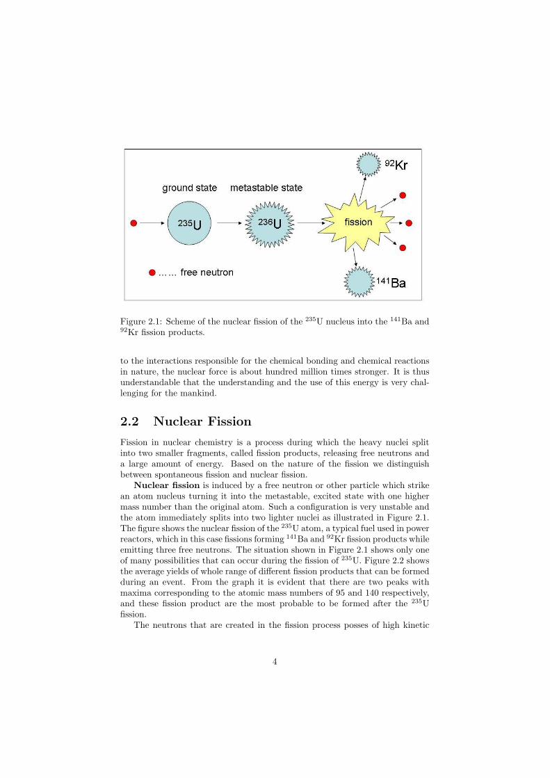
Figure 2.1: Scheme of the nuclear fission of the 235U nucleus into the 141Ba and92Kr fission products.

to the interactions responsible for the chemical bonding and chemical reactionsin nature, the nuclear force is about hundred million times stronger. It is thusunderstandable that the understanding and the use of this energy is very chal-lenging for the mankind.

2.2 Nuclear Fission

Fission in nuclear chemistry is a process during which the heavy nuclei splitinto two smaller fragments, called fission products, releasing free neutrons anda large amount of energy. Based on the nature of the fission we distinguishbetween spontaneous fission and nuclear fission.

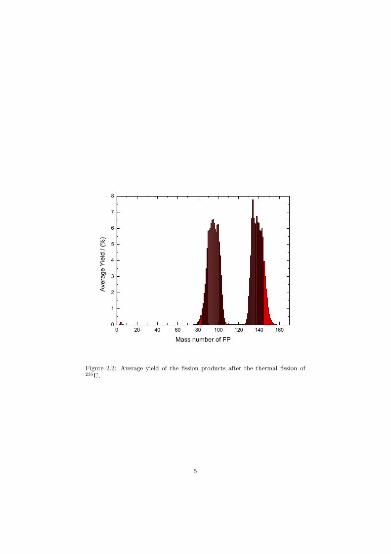
Nuclear fission is induced by a free neutron or other particle which strikean atom nucleus turning it into the metastable, excited state with one highermass number than the original atom. Such a configuration is very unstable andthe atom immediately splits into two lighter nuclei as illustrated in Figure 2.1.The figure shows the nuclear fission of the 235U atom, a typical fuel used in powerreactors, which in this case fissions forming 141Ba and 92Kr fission products whileemitting three free neutrons. The situation shown in Figure 2.1 shows only oneof many possibilities that can occur during the fission of 235U. Figure 2.2 showsthe average yields of whole range of different fission products that can be formedduring an event. From the graph it is evident that there are two peaks withmaxima corresponding to the atomic mass numbers of 95 and 140 respectively,and these fission product are the most probable to be formed after the 235Ufission.

The neutrons that are created in the fission process posses of high kinetic

4

0 20 40 60 80 100 120 140 1600

1

2

3

4

5

6

7

8

Ave

rag

e Y

ield

/ (

%)

Mass number of FP

Figure 2.2: Average yield of the fission products after the thermal fission of235U.

5

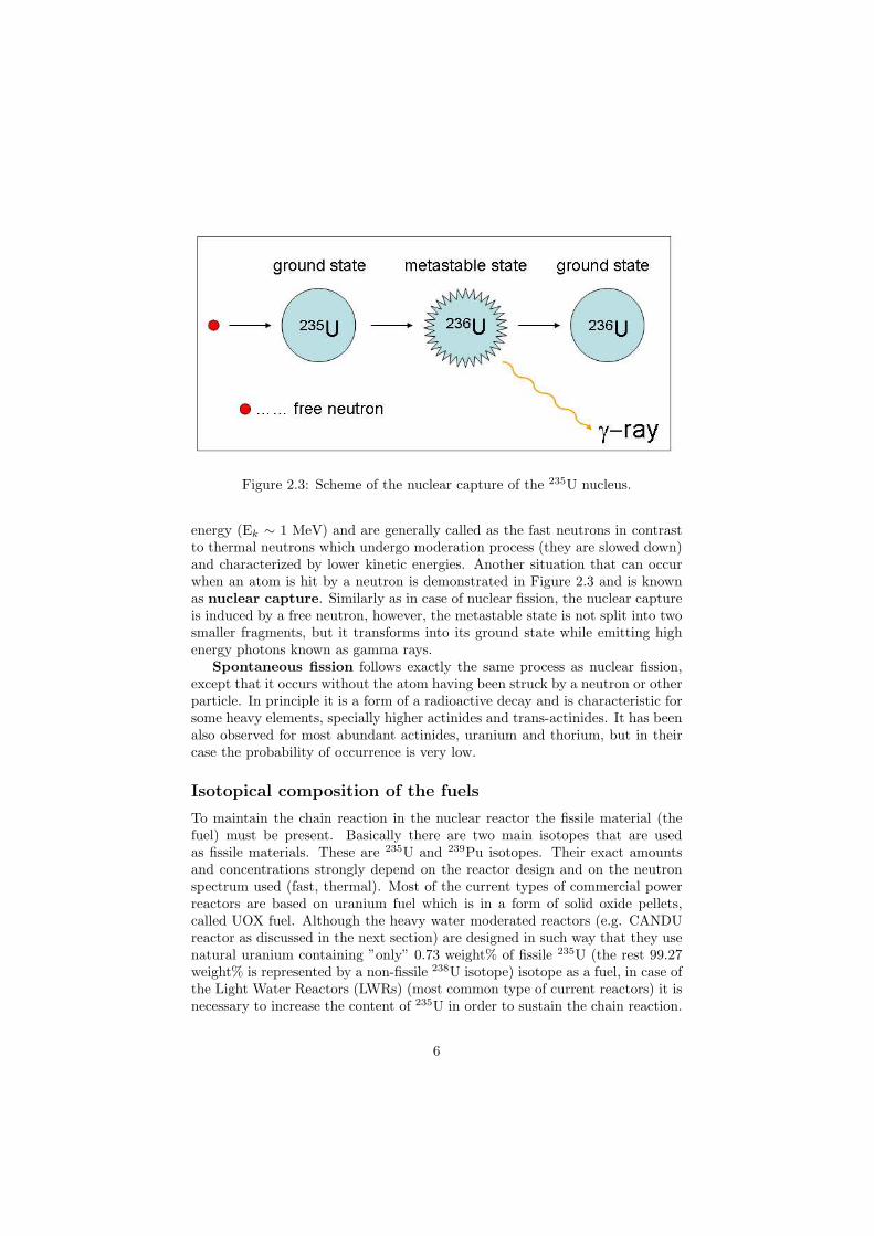
Figure 2.3: Scheme of the nuclear capture of the 235U nucleus.

energy (Ek ∼ 1 MeV) and are generally called as the fast neutrons in contrastto thermal neutrons which undergo moderation process (they are slowed down)and characterized by lower kinetic energies. Another situation that can occurwhen an atom is hit by a neutron is demonstrated in Figure 2.3 and is knownas nuclear capture. Similarly as in case of nuclear fission, the nuclear captureis induced by a free neutron, however, the metastable state is not split into twosmaller fragments, but it transforms into its ground state while emitting highenergy photons known as gamma rays.

Spontaneous fission follows exactly the same process as nuclear fission,except that it occurs without the atom having been struck by a neutron or otherparticle. In principle it is a form of a radioactive decay and is characteristic forsome heavy elements, specially higher actinides and trans-actinides. It has beenalso observed for most abundant actinides, uranium and thorium, but in theircase the probability of occurrence is very low.

Isotopical composition of the fuels

To maintain the chain reaction in the nuclear reactor the fissile material (thefuel) must be present. Basically there are two main isotopes that are usedas fissile materials. These are 235U and 239Pu isotopes. Their exact amountsand concentrations strongly depend on the reactor design and on the neutronspectrum used (fast, thermal). Most of the current types of commercial powerreactors are based on uranium fuel which is in a form of solid oxide pellets,called UOX fuel. Although the heavy water moderated reactors (e.g. CANDUreactor as discussed in the next section) are designed in such way that they usenatural uranium containing ”only” 0.73 weight% of fissile 235U (the rest 99.27weight% is represented by a non-fissile 238U isotope) isotope as a fuel, in case ofthe Light Water Reactors (LWRs) (most common type of current reactors) it isnecessary to increase the content of 235U in order to sustain the chain reaction.

6

This is achieved by uranium enrichment and the typical concentration of 235Uin the reactor grade uranium is ∼ 3-4 weight%.

Another widely used nuclear fuel is a mixed oxide of uranium and plutonium,called MOX fuel. In principle it is an alternative to the UOX fuels with similartotal concentrations (∼ 3-4 weight%) of the fissile isotopes (235U and 239Pu).The advantage of using the MOX fuel is mainly the possibility of using separatedfissile 239Pu which is daily produced in the nuclear reactors by neutron capturingof the non-fissile 238U nuclide.

2.3 The Nuclear Fuel Cycle

The nuclear fuel cycle consists of several stages. The primary stage, also calledfront end includes the preparation processes like mining, enrichment and fuelfabrication. It continues through the service period, during which the fuel isinstalled in the nuclear reactor and is used for energy production. The lastperiod of the fuel life time is called back end and consists of the fuel managementafter its operation in the reactor. At this stage the fuel can be either reprocessedor disposed as a nuclear waste. If the fuel is directly disposed as a nuclear wastethe fuel cycle is referred to as an open fuel cycle, also known as once-through fuelcycle. In case that the fuel is reprocessed the fuel cycle is referred to as a closedfuel cycle. During the reprocessing the fission products, minor actinides, andreprocessed uranium are separated from plutonium, which is then fabricatedinto the MOX fuel. The fission products together with the minor actinidesare disposed as a nuclear waste, but due to the very long half-life of someminor actinides (in order of 106 years) no one can guarantee that the storageassembly would resist the environmental conditions over such period of timeand the disposal is not definite. Nevertheless, this problem will be solved withthe introduction of the advanced fast reactor concepts where it is planned tore-use these minor actinides as part of the fuel.

2.4 Nuclear Reactors

Current types of nuclear power reactors

A nuclear reactor is a device in which the nuclear chain reaction is initiated,controlled and sustained at constant rate. In order to keep the chain reaction,there must be such an amount of fuel in such space configuration that the wholeassembly is in supercritical state. It is a state at which more neutrons areproduced during the nuclear fission of the fissile material than consumed by thecapturing of the atom nuclei. A numerical measure of the supercritical state isdependent on the neutron multiplication factor, k, where:

k = f − l (2.2)

where f is the average amount of neutrons released during the fission and l is theaverage amount of neutrons being escaped from the system or being consumed

7

during non-fissile processes. When k > 1 the mass is supercritical and the rateof fission increases. When k = 1 the mass is critical and corresponds to theequilibrium fission reaction where there is no increase or decrease of neutronpopulation. When k < 1 the mass is subcritical. At this state the populationof neutrons introduced to the system will exponentially decrease.

Based on the neutron spectrum the nuclear reactors can be divided into twomain groups. First group are the fast reactors in which the fission chain reactionis sustained by the fast neutrons, neutrons that posses of high kinetic energy.At the moment there are only few reactors of this kind used for electricity pro-duction (e.g. russian BN-600). Most of the fast reactors currently being underoperation are either prototypes (e.g. french Phenix reactor) or test reactors.The second group consists of thermal reactors characterized by a thermal neu-tron spectrum. In these reactors the neutrons are first slowed down before theystrike a fissile atom. This is done by introducing a moderator, a medium whichreduces the velocity of fast neutrons by absorbing part of their kinetic energy.Mostly used moderators in current power reactors are light water, graphite orheavy water. It is the thermal reactors that are widely used all over the worldto produce the electric power.

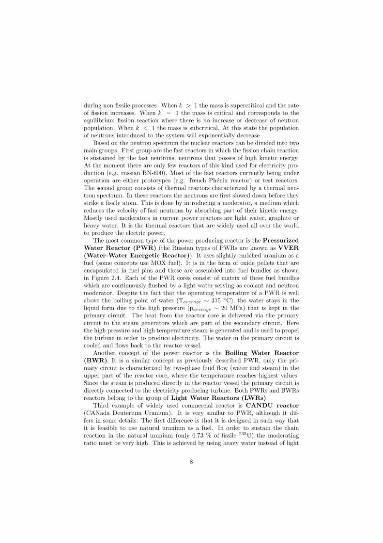
The most common type of the power producing reactor is the PressurizedWater Reactor (PWR) (the Russian types of PWRs are known as VVER(Water-Water Energetic Reactor)). It uses slightly enriched uranium as afuel (some concepts use MOX fuel). It is in the form of oxide pellets that areencapsulated in fuel pins and these are assembled into fuel bundles as shownin Figure 2.4. Each of the PWR cores consist of matrix of these fuel bundleswhich are continuously flushed by a light water serving as coolant and neutronmoderator. Despite the fact that the operating temperature of a PWR is wellabove the boiling point of water (Taverage ∼ 315 C), the water stays in theliquid form due to the high pressure (paverage ∼ 20 MPa) that is kept in theprimary circuit. The heat from the reactor core is delivered via the primarycircuit to the steam generators which are part of the secondary circuit. Herethe high pressure and high temperature steam is generated and is used to propelthe turbine in order to produce electricity. The water in the primary circuit iscooled and flows back to the reactor vessel.

Another concept of the power reactor is the Boiling Water Reactor(BWR). It is a similar concept as previously described PWR, only the pri-mary circuit is characterized by two-phase fluid flow (water and steam) in theupper part of the reactor core, where the temperature reaches highest values.Since the steam is produced directly in the reactor vessel the primary circuit isdirectly connected to the electricity producing turbine. Both PWRs and BWRsreactors belong to the group of Light Water Reactors (LWRs).

Third example of widely used commercial reactor is CANDU reactor(CANada Deuterium Uranium). It is very similar to PWR, although it dif-fers in some details. The first difference is that it is designed in such way thatit is feasible to use natural uranium as a fuel. In order to sustain the chainreaction in the natural uranium (only 0.73 % of fissile 235U) the moderatingratio must be very high. This is achieved by using heavy water instead of light

8

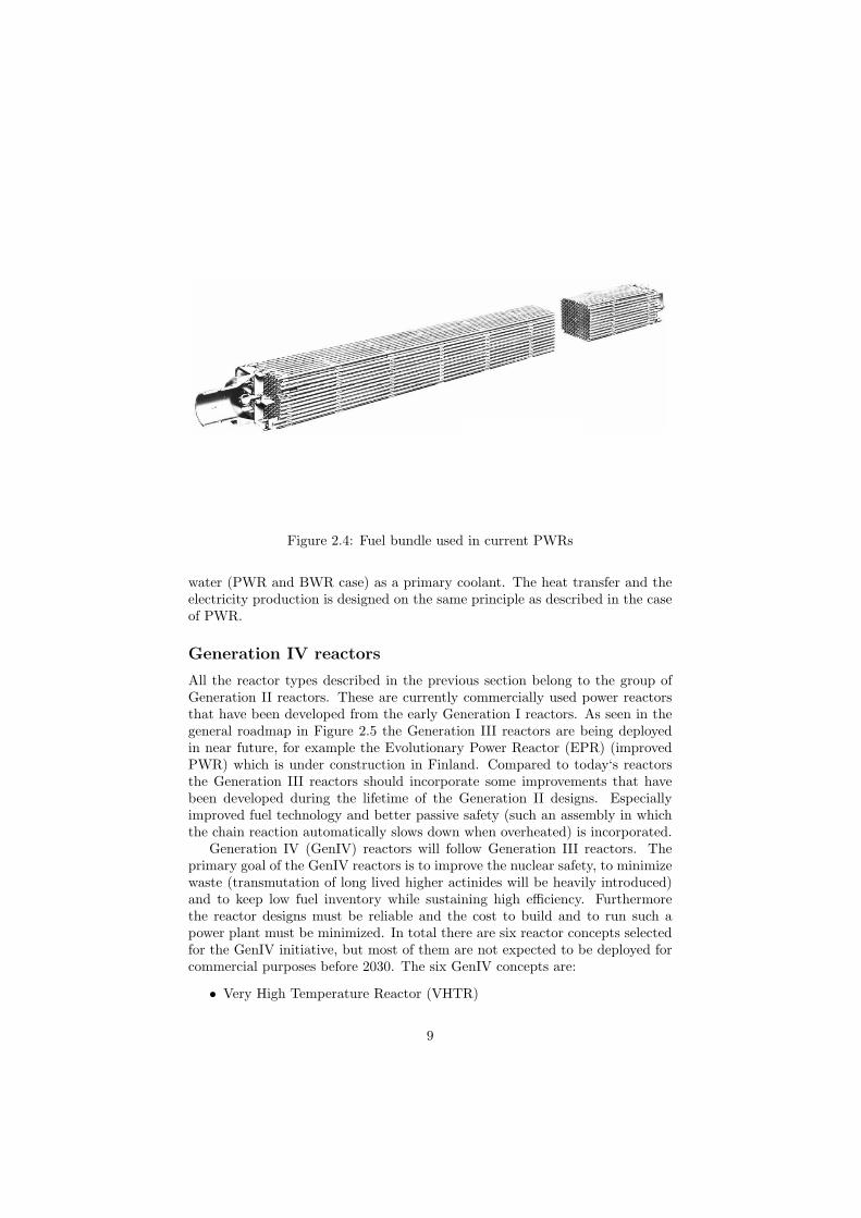
Figure 2.4: Fuel bundle used in current PWRs

water (PWR and BWR case) as a primary coolant. The heat transfer and theelectricity production is designed on the same principle as described in the caseof PWR.

Generation IV reactors

All the reactor types described in the previous section belong to the group ofGeneration II reactors. These are currently commercially used power reactorsthat have been developed from the early Generation I reactors. As seen in thegeneral roadmap in Figure 2.5 the Generation III reactors are being deployedin near future, for example the Evolutionary Power Reactor (EPR) (improvedPWR) which is under construction in Finland. Compared to today‘s reactorsthe Generation III reactors should incorporate some improvements that havebeen developed during the lifetime of the Generation II designs. Especiallyimproved fuel technology and better passive safety (such an assembly in whichthe chain reaction automatically slows down when overheated) is incorporated.

Generation IV (GenIV) reactors will follow Generation III reactors. Theprimary goal of the GenIV reactors is to improve the nuclear safety, to minimizewaste (transmutation of long lived higher actinides will be heavily introduced)and to keep low fuel inventory while sustaining high efficiency. Furthermorethe reactor designs must be reliable and the cost to build and to run such apower plant must be minimized. In total there are six reactor concepts selectedfor the GenIV initiative, but most of them are not expected to be deployed forcommercial purposes before 2030. The six GenIV concepts are:

• Very High Temperature Reactor (VHTR)

9

Figure 2.5: Time evolution of the nuclear reactors

• Supercritical Water Cooled Reactor (SCWR)

• Gas Cooled Fast Reactor (GFR)

• Sodium Cooled Fast Reactor (SFR)

• Lead Cooled Fast Reactor (LFR)

• Molten Salt Reactor (MSR)

The VHTR is a thermal reactor that is graphite-moderated and uses heliumgas as a primary coolant. It uses a once-through uranium fuel cycle (open fuelcycle), meaning that the spent fuel is not reprocessed. The strength of VHTRdesign is in the high outlet temperature of the reactor core which can reach1000 C. Thus its heat can be directly used to produce the hydrogen via theiodine-sulfur cycle [1] or for desalination of water. Due to the high operationaltemperature, this reactor posses of high efficiency.

The SCWR is another thermal reactor concept that is based on the once-through uranium fuel cycle, as similar as the VHTR. The coolant is a light waterin supercritical state (T > 374 C) and the primary loop is directly connectedto the turbine for electricity production, similarly as in case of BWR. The maindifference to the BWR is the state of the working fluid, which in this case iscomposed of only one phase. Basically SCWR operates at much higher temper-atures than PWRs or BWRs, and therefore its thermal efficiency is higher.

The reference GFR design is a helium cooled system based on the fast neu-tron spectrum with an outlet reactor temperature of 850 C. The primary circuit

10

is directly connected to the gas turbine for electricity production. The exactfuel form is not clearly defined yet, but it will be most likely designed in suchway that the core will have high fissile material content with addition of a fer-tile material, which will breed more fuel by neutron capturing. It is importantto note that the temperatures exceeding 850 C are high enough for the ther-mochemical production of hydrogen, thus this reactor concept is possible to beused for this purpose as well as VHTR, however, different medium than heliumgas should be used for heat transfer between the reactor core and the hydrogenplant. For this purpose the molten salts are serious candidates. Higher heatcapacity, density and thermal conductivity are required for such heat trans-fer salts. As good candidates flinak (eutectic composition of the LiF-NaF-KFsystem) or the eutectic composition of the NaNO3-KNO3 system are considered.

The SFR is another fast reactor design. Concerning the fuel there are twomain options: One is based on the uranium-plutonium-minor actinide zirconiumalloy, the second one considers mixed uranium-plutonium oxide fuel. Both con-cepts employ full actinide recycle (closed fuel cycle) and the reference coolant ismolten sodium. In order to avoid the contact between sodium and water, therewill be an intermediate loop between the primary circuit and the steam gen-erator which could be operated with a molten fluoride salt or molten nitrate salt.

The LFR is a reactor concept based on a fast neutron spectrum. It usesmolten lead or lead-bismuth eutectic melt as a coolant, and a closed fuel cy-cle. The fuel is metallic, oxide or nitride-based and contains fertile uranium (tobreed more fuel) and actinides as fissile material. The reactor outlet tempera-ture is 550 C, but with the use of advanced materials it can be increased totemperatures over 850 C. In that case it would be possible to use the LFR fordirect hydrogen production.

The MSR is the sixth reactor type of the Generation IV initiatives andsince the thermodynamic description of the MSR fuel is the main subject ofthis study the whole concept is described in more details in the next section.

2.5 Molten Salt Reactor (MSR)

MSR description

In a molten salt reactor the nuclear fuel is dissolved in an inorganic liquid(most likely a mixture of fluorides) that is pumped at a low pressure throughthe reactor vessel and the primary circuit and thus also serves as the primarycoolant. The heat generated by the fission process is transferred to a secondarycoolant in a heat exchanger. This secondary coolant is generally a molten saltalso. Figure 2.6 shows the MSR concept as designed by ORNL.

11

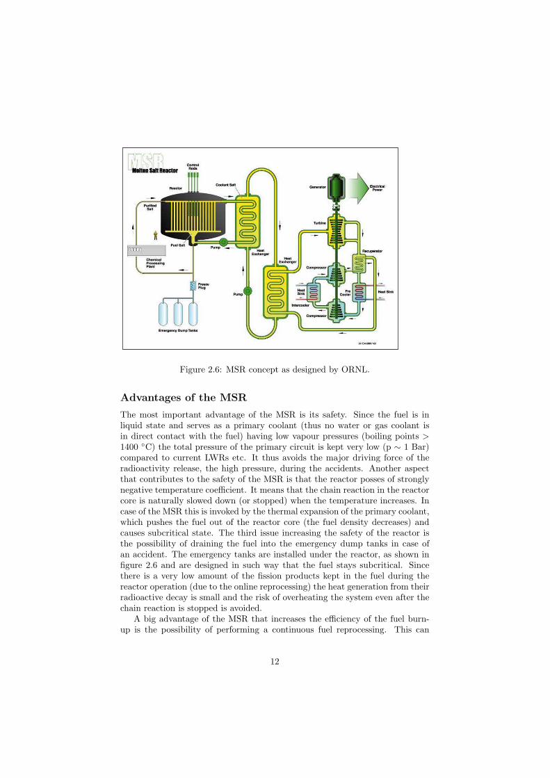
Figure 2.6: MSR concept as designed by ORNL.

Advantages of the MSR

The most important advantage of the MSR is its safety. Since the fuel is inliquid state and serves as a primary coolant (thus no water or gas coolant isin direct contact with the fuel) having low vapour pressures (boiling points >1400 C) the total pressure of the primary circuit is kept very low (p ∼ 1 Bar)compared to current LWRs etc. It thus avoids the major driving force of theradioactivity release, the high pressure, during the accidents. Another aspectthat contributes to the safety of the MSR is that the reactor posses of stronglynegative temperature coefficient. It means that the chain reaction in the reactorcore is naturally slowed down (or stopped) when the temperature increases. Incase of the MSR this is invoked by the thermal expansion of the primary coolant,which pushes the fuel out of the reactor core (the fuel density decreases) andcauses subcritical state. The third issue increasing the safety of the reactor isthe possibility of draining the fuel into the emergency dump tanks in case ofan accident. The emergency tanks are installed under the reactor, as shown infigure 2.6 and are designed in such way that the fuel stays subcritical. Sincethere is a very low amount of the fission products kept in the fuel during thereactor operation (due to the online reprocessing) the heat generation from theirradioactive decay is small and the risk of overheating the system even after thechain reaction is stopped is avoided.

A big advantage of the MSR that increases the efficiency of the fuel burn-up is the possibility of performing a continuous fuel reprocessing. This can

12

be done either on-line or in batches and the concept is proposed in such waythat the reprocessing chemical plant is installed on site of the nuclear reactor(no transportation of the fuel). A position of this reprocessing chemical plantwithin the MSR unit is shown in Figure 2.6. The goal of the fuel clean-up is toseparate the fission products from the fuel and put them into the nuclear waste,while the cleaned fuel is sent back into the primary circuit. It is very importantto make this separation, because most of the fission products have a very highneutron capture cross section and thus slow down the chain reaction. Due tothis online reprocessing a low initial inventory of the fissile material is possible.Moreover, it is also possible to profit from the neutron economy and design theMSRs as breeder reactors that produce more fuel than consume.

The MSR can be designed as an actinide burner reactor. It would thus bepossible to inject the minor actinides containing nuclear waste from the currenttypes of power reactors into the MSR fuel cycle and transmute these long livedisotopes into the short lived fission products. The transmutation process is verychallenging for the nuclear scientists because it would help to solve the problemof the final nuclear waste disposal which is at the moment considered as a majordraw-back of nuclear power due to the presence of the long lived actinides thatneed millions of years before they decay into the stable isotopes.

Another characteristic of the MSR is no radiation damage of the fuel dueto its liquid state. This is of importance since in the solid fuels the radiationdamage causes swelling of the fuel pins and these must be than replaced by thenew ones.

The last, but not least issue among the big advantages of the MSR is apossibility to use it for a direct hydrogen production. This is however still asubject of investigation, because special alloys would be required for structuralmaterial in order to avoid the corrosion of the fluoride salts at high temperatures.

Drawbacks of the MSR

The main disadvantage of the MSR is the corrosion of the structural materialby the molten fluoride salt, which can occur at high temperatures. However, aprofound investigation is being carried out in this field of science in order to finda compatible alloy which would serve as a structural material and would not bedamaged during the operational lifetime of the reactor. The nickel based alloys,namely Hastelloy N alloy is very promising. The MSRE (see next subsection) hasbeen based on this alloy and operated successfully over four year period with nocorrosion damage. In that case the reactor outlet temperature was 654 C, morethan 150 C less than the temperature necessary for direct hydrogen production(above 800 C). At higher temperatures the corrosion rate increases and newalloys, compatible with the molten fluoride salt must be invented.

History of the MSR

The first proposal for a molten-salt reactor dates from the 1940s when Bettisand Briant proposed it for aircraft propulsion [2]. A substantial research pro-

13

gramme was started at Oak Ridge National Laboratory (ORNL) in the USA todevelop this idea, culminating in the Aircraft Reactor Experiment (ARE) thatwas critical during several days in 1954. For ARE a mixture of NaF-ZrF4 wasused as carrier of the fissile UF4 [3, 4].

In the second half of the 1950s the molten salt technology was transferredto the civilian nuclear programme of the US. At that time many reactor con-cepts were being studied and the interest in breeder reactors was large. It wasrecognized that the molten salt reactor would be ideal for thermal breeding ofuranium from thorium [2] and the Molten Salt Reactor Experiment (MSRE)was started at ORNL to demonstrate the operability of molten-salt reactors.Because of the breeding aspect, the neutron economy in the reactor was consid-ered of key importance and 7LiF-BeF2 (flibe), with 5 % ZrF4 as oxygen getter,was selected as fuel carrier because of the very low neutron-capture cross sec-tions of 7Li and Be. The MSRE was a graphite-moderated reactor of 8 MWththat operated from 1965-1969. Three different fissile sources were used: 235UF4,233UF4 and 239PuF3. flibe was used as coolant in the secondary circuit. Theresults of MSRE, which have been reported in great detail [5], revealed that theselected materials (fuel, structurals) all behaved well and that the equipmentbehaved reliably. In that respect it was very successful.

After the MSRE a design for a prototype Molten Salt Breeder Reactor(MSBR) was made by ORNL in early 1970s [6], in which a continuous repro-cessing of the fuel was foreseen to reduce the neutron loss by capture in fissionproducts. The program was stopped in 1976, in favor of the liquid metal cooledfast reactor [2] although the technology was considered promising, but recog-nizing the technological problems that had to be solved. The MSBR design wasa 2250 MWth reactor, optimized to breed 233U from thorium in a single fluidsystem. Online pyrochemical reprocessing was planned to clean the fuel solventfrom the neutron absorbing fission products. Nevertheless interruption of reac-tor operation was planned every four years to replace the graphite moderator, asexperiments had revealed significant swelling of graphite due to radiation dam-age. Because of the online clean up of the fuel, the zirconium addition to thefuel was not necessary and flibe could be used as carrier of the fertile (ThF4)and fissile elements (UF4). As secondary coolant, a NaF-NaBF4 mixture (0.08-0.92 molar composition) was foreseen because the tritium retention of this saltis much better than flibe.

Fuel concepts in the MSR

In the section above the MSBR concept has been mentioned as a graphite mod-erated reactor that has been based on the 7LiF-BeF2-ThF4-UF4 system [6]. Thisfuel composition based on the flibe matrix still remains as an ideal candidatewhen the MSR is designed as a thermal breeder reactor (moderated reactor).In this case the neutron economy is very critical and only the isotopes withvery low neutron capture cross section in the thermal spectrum can be consid-ered as part of the fuel matrix. Thus 7LiF and BeF2 are the compounds ofconsideration.

14

Nowadays the non-moderated (fast) (although there is no moderating mediumin the reactor core, the neutrons emitted during the fission are partially moder-ated by the fluorine atom which is part of the fuel matrix - therefore the ”non-moderated” rather than ”fast” term is preferred in case of the MSR) reactorsare of higher interest for its possibility of transmuting the long lived actinidesproduced mostly in the thermal reactors. The transmutation is effective onlywhen initiated by high energy neutrons (epithermal or fast spectrum), becauseat that energy all the minor actinides are fissionable. Moreover the fission tocapture ratio for these nuclides is much higher in the fast than in the thermalspectrum. Another advantage of the non-moderated reactor is the absence ofthe graphite (as a moderator in the thermal MSR) in the reactor core which isvery inclinable for radiation damage and must be periodically replaced.

In case of the MSR there are two main directions of the non-moderated(fast) reactor concepts. First is an actinide burner design based on the RussianMOSART (MOlten Salt Actinide Recycler & Transmuter) concept [7] which usesthe 7LiF-NaF-BeF2-AnF3 system as a fuel. ’An’ is mainly represented by 239Puwith some addition of minor actinides. The second one is an innovative conceptcalled TMSR-NM (Non Moderated Thorium Molten Salt Reactor) that hasbeen developed by CNRS-Grenoble in France [8–11]. The fuel in this concept isbased on the 7LiF-232ThF4 matrix with the addition of the actinide fluorides asa fissile material. 232ThF4 is a fertile material that is bred to fissile 233UF4 by aneutron capture and consecutive beta decay. There are two initial fissile choicesin the TMSR-NM concept, (1) the 233U-started TMSR and (2) the transuranic-started TMSR with the mix of 87.5% of Pu (238Pu 2.7%, 239Pu 45.9%, 240Pu21.5%, 241Pu 10.7% and 242Pu 6.7%), 6.3% Np, 5.3% of Am and 0.9% of Cm,corresponding to the transuranic elements composition of an UOX fuel after oneuse in a PWR and five years of storage [12].

One of the very recent designs of the MSR is the REBUS-3700 concept whichis based on the chloride salt as a fuel. It is a fast breeder reactor which hasbeen proposed by Mourogov and Bokov [13] and it is based on a U-Pu cycle,where U and Pu are present in the form of trichlorides dissolved in a matrixof liquid NaCl. In general the chlorides have higher vapor pressures and lowerthermodynamic stability at high temperatures compared to fluorides, but onthe other hand, they are less aggressive against the structural materials andtheir melting points are lower. Therefore, more fissile material can be dissolvedin the matrix and that is necessary for fast breeder reactor designs. However,the chlorides can only be used in fast reactors and not in thermal ones, due tothe relatively high parasitic neutron-capture cross-section of the chlorine atom.

Other nuclear applications of the molten salts

Molten salts are not only used as fuels (primary circuit of a MSR), but they canbe potentially used as secondary coolants in the MSR or as primary coolants insome of the advanced reactor concepts, as well as the heat transfer salts betweenthe nuclear reactor and the hydrogen production plant.

Probably the most suitable candidate as a secondary coolant of the MSR

15

is the eutectic composition of the NaF-NaBF4 system, a coolant that has beenused in the MSBR project. As an alternative the LiF-BeF2 system or the KF-KBF4 system is considered. For advanced high temperature reactors that arebased on the thermal spectrum the 7LiF-BeF2 (flibe) system is very promisingcandidate for a secondary coolant. In this case it is demanding to have highpurity of 7Li isotope (∼99.995 weight%), because the other naturally occurringlithium isotope, 6Li, is a neutron poison due to its very high neutron capturecross section and must be avoided from the reactor core. For secondary coolantsthis restriction does not have to be fulfilled because this salt is not in directcontact with the reactor core and does not slow down the chain reaction. Inthat case the natural isotopical composition of lithium (7.6 weight% of 6Li and92.4 weight% of 7Li) can be used.

As a secondary coolant for a fast reactor the eutectic composition of theLiCl-NaCl-MgCl2 system is proposed. In this case the salt is based on the chlo-rides which have higher neutron capture cross section than fluorides, howeverin the fast spectrum reactors the neutron economy is not as sensitive as in thethermal ones and chlorides can be of potential use. As discussed in the previoussection for a heat transfer salts the flinak system (eutectic composition of theLiF-NaF-KF system) or the eutectic composition of the NaNO3-KNO3 systemare considered. As an alternative the eutectic composition of the LiCl-KCl-MgCl2 system is proposed.

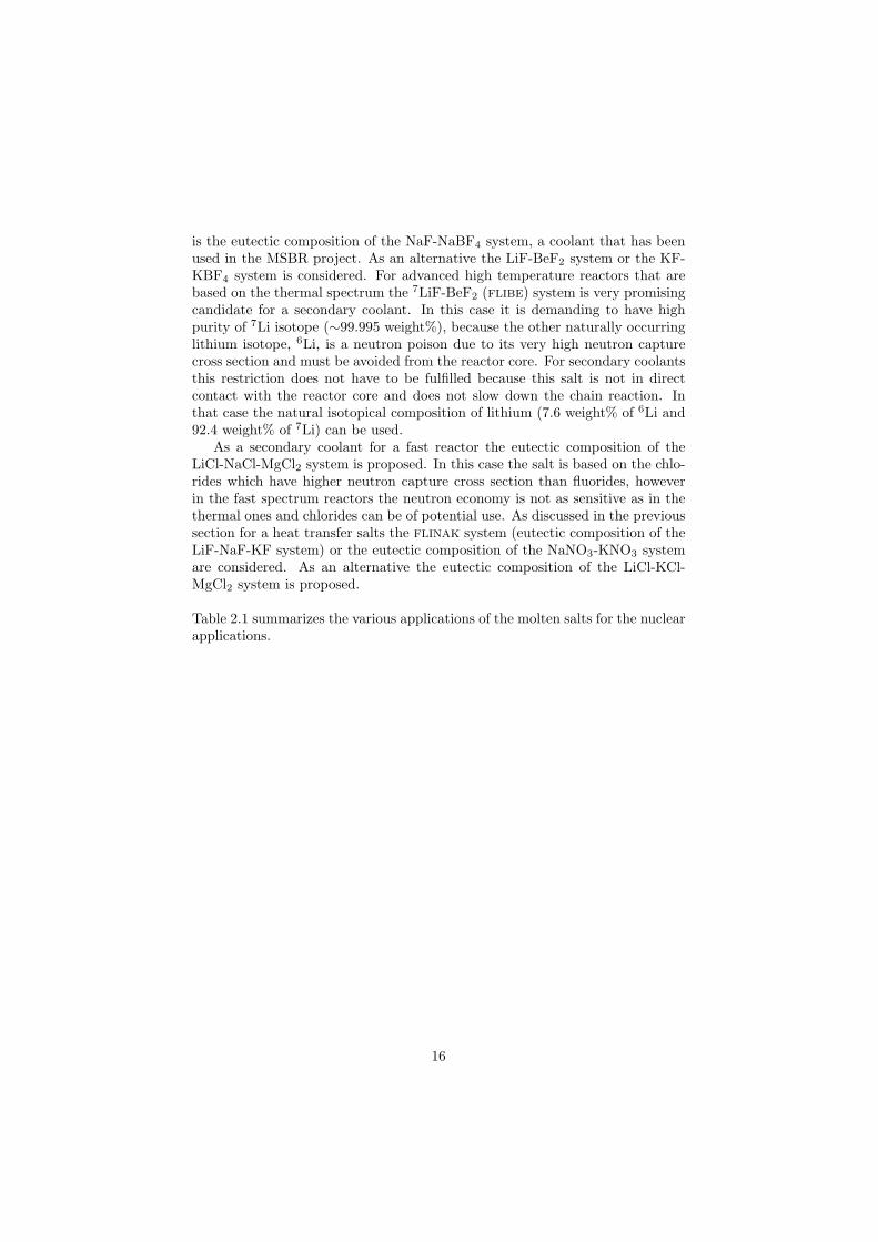
Table 2.1 summarizes the various applications of the molten salts for the nuclearapplications.

16

Table 2.1: The various applications of molten salts in the nuclear reactor science.Reactor Neutron Application Primary choice Alternative(s)type spectrumMSR Breeder Thermal Fuel 7LiF-BeF2-AnF4

Fast Fuel 7LiF-AnF4

Coolant NaF-NaBF4 LiF-BeF2, KF-KBF4

MSR Burner Fast Fuel LiF-NaF-BeF2-AnF3 LiF-NaF-KF-AnF3

AHTR ∗ Thermal Coolant 7LiF-BeF2

VHTR Thermal Heat transfer LiF-NaF-KF LiCl-KCl-MgCl2FR Fast Coolant LiCl-NaCl-MgCl2SFR Fast Heat transfer NaNO3-KNO3

∗ AHTR .... Advanced High Temperature Reactor

17

Chapter 3

Thermodynamics

It has been shown in the previous chapter which salt systems are the maincandidates for the nuclear applications. Basically the choice has been made ona basis of the salt properties that must fulfill following criteria (the solubilityfor actinides and the neutronic properties do not apply to coolants and the heattransfer salts):

• Low melting point.

• Low vapour pressure at the operating temperature of the reactor.

• Wide range of solubility for actinides.

• Thermodynamic stability up to high temperatures.

• Stability to radiation (no radiolytic decomposition).

• Low neutron capture cross section.

• Compatibility with nickel-based alloys (Ni-Mo-Cr-Fe) that can be used asstructural materials (Hastelloy).

The low melting temperature is required because the lower the melting tem-perature the lower the risk of the system to freeze at certain circumstances.Another reason to ensure a low melting temperature is related to the corrosioneffects. If the salt melts at higher temperatures the operation temperature ofthe reactor must be also raised and the rate of the corrosion of the structuralmaterial by the salt increases. It is very important that the reactor inlet tem-perature is at least 50 K higher than the melting point of the salt in order tokeep a safety margin. It avoids the risk of solid precipitation which could cause,in case of the actinide rich solid precipitates, local supercriticality and result inlocal hot spots.

The low vapor pressure of the salt is not only required to keep the wholereactor circuit at low pressure, but it also avoids the change of the molten saltcomposition which can occur due to the incongruent vaporization.

18

The main objective of this work is a thermodynamic description of the flu-oride and chloride systems that are relevant for nuclear applications (fuels,coolants or heat transfer salts), based on experiments and modelling. For areactor design it is very important to have a thermodynamic description ofthese systems, because the melting behavior, the vapour pressure, thermody-namic stability at high temperatures or the solubility for actinides in the matrixof the fuel can be obtained based on these results.

It is also impossible to measure every single composition one might be in-terested in, so the solution is to develop a model that would describe the wholesystem. Moreover it is much easier to optimize the fuel (coolant or heat transfersalt) composition based on the knowledge of the phase diagrams.

3.1 Thermodynamic modelling

The main outcome of the thermodynamic modelling is the assessment of thephase diagram. It is a graph that shows stable phase fields as a function of anyvariable (temperature, pressure, composition, electric potential etc.). The mostcommon type is a T -x phase diagram which shows the stable phase fields as afunction of temperature and composition. Basically, based on the knowledgeof a T -x phase diagram one can deduce at what temperature a certain fuelor coolant composition melts, boils or decomposes. It is very important tonote that departures from equilibrium can occur in any real system, however aknowledge of the equilibrium state is usually the starting point to understand thebehaviour of certain system at given conditions. The non-equilibrium state is theconsequence of the kinetic aspects (e.g. supercooling during the glass formation)and are usual for low temperatures. At higher temperatures, typically closeto the melting temperatures and higher the thermodynamics (the equilibriumstate) becomes dominant.

In thermodynamics a simple rule applies which states that the configurationof any system which possesses a lower Gibbs energy is more stable than theone with higher energy. Hence in order to describe a T -x phase diagram, aknowledge of the Gibbs energy equations of all phases and the Gibbs equationsof mixing, in case of the presence of solutions, are required. If these data are notknown they need to be obtained by performing a thermodynamic assessment.This is usually done (and has been done in this study as well) according to theCALPHAD method including the critical review of all available data of interest(mixing enthalpies of the solutions, solidus and liquidus points etc.) followedby the optimization of the unknown data in order to obtain the best possiblefit between the experimental values and the calculated ones. In case of thefluoride and chloride systems assessed in this study, these unknown parametersare mostly the excess properties of the solutions and the thermodynamic data ofsome intermediate compounds. All the thermodynamic calculations presentedin this study have been performed using the FactSage software [14]. Figure 3.1shows an example of a T -x binary phase diagram optimized in this study. It isa LiF-NaF system and as the figure indicates, a very good agreement between

19

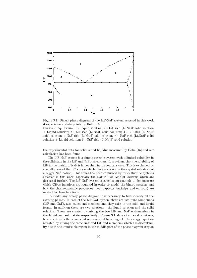
Figure 3.1: Binary phase diagram of the LiF-NaF system assessed in this work experimental data points by Holm [15]Phases in equlibrium: 1 - Liquid solution; 2 - LiF rich (Li,Na)F solid solution+ Liquid solution; 3 - LiF rich (Li,Na)F solid solution; 4 - LiF rich (Li,Na)Fsolid solution + NaF rich (Li,Na)F solid solution; 5 - NaF rich (Li,Na)F solidsolution + Liquid solution; 6 - NaF rich (Li,Na)F solid solution

the experimental data for solidus and liquidus measured by Holm [15] and ourcalculation has been found.

The LiF-NaF system is a simple eutectic system with a limited solubility inthe solid state in the LiF and NaF rich corners. It is evident that the solubility ofLiF in the matrix of NaF is larger than in the contrary case. This is explained bya smaller size of the Li+ cation which dissolves easier in the crystal sublattice ofa bigger Na+ cation. This trend has been confirmed by other fluoride systemsassessed in this work, especially the NaF-KF or KF-CsF systems which arediscussed further. The LiF-NaF system is taken as an example to demonstratewhich Gibbs functions are required in order to model the binary systems andhow the thermodynamic properties (heat capacity, enthalpy and entropy) arerelated to these functions.

To model any binary phase diagram it is necessary to first identify all theexisting phases. In case of the LiF-NaF system there are two pure compounds(LiF and NaF), also called end-members and they exist in the solid and liquidforms. In addition there are two solutions - the liquid solution and the solidsolution. These are created by mixing the two LiF and NaF end-members inthe liquid and solid state respectively. Figure 3.1 shows two solid solutions,however, this is the same solution described by a single Gibbs energy equation(created by mixing the same NaF and LiF end-members) which has discontinu-ity due to the immiscible region in the middle part of the phase diagram (region

20

4 in Figure 3.1).

Pure compounds - condensed phases

To describe the Gibbs energy equation of pure compounds as a function oftemperature it is necessary to know the enthalpy and entropy contributions aswritten in the equation below:

G(T ) = H(T )− T · S(T ) (3.1)

It is usually difficult to obtain the enthalpy and entropy functions directly andtherefore Equation 3.1 can be written as a function of the standard enthalpyof formation ∆fH0(298), the standard absolute entropy S0(298), both referredto a standard state temperature at T = 298.15 K (in this text this value issimplified to 298 K) and the heat capacity function of temperature Cp(T ) asgiven in the equation below:

G(T ) = ∆fH0(298)− S0(298)T +

∫ T

298

Cp(T )dT − T

∫ T

298

(

Cp(T )

T

)

dT (3.2)

Note that the above equation describes the Gibbs function for temperatureshigher than 298 K. However this temperature range is relevant when consider-ing the salt behaviour above the ambient temperature. If one needs to describethe Gibbs functions from absolute temperature, the ∆fH0(298) term in Equa-tion 3.2 must be replaced by the ∆fH0(0) term and since the absolute entropyat T=0 K is equal to zero, the S0(298) term is eliminated. Consequently thelower limits of the two integrals in Equation 3.2 are set to 0.

Equation 3.2 can be also written in an analytical form (in some cases theinput form to the FactSage software [14]), in which the Cp contribution is rep-resented by a polynomial function of T as it is shown in Equation 3.3. In thisequation a and b are constants.

G(T ) = ∆fH0(298)− S0(298)T +∑

i=n

aiTi + bT ln(T ) (3.3)

The standard enthalpy of any compound is equal to the reaction enthalpy ofthe compound formation from the pure elements in their standard states (stablephase at p = 100000 Pa). An example is shown for a case of LiF on the followingformation reaction:

T = 298 K : Li(crystal) +1

2F2(gas) → LiF (crystal) (3.4)

The standard reaction enthalpy of Equation 3.4 is written as:

∆rH0LiF (298) = ∆fH0

LiF (crystal)(298)−H0Li(crystal)(298)−

1

2H0

F2(gas)(298)

(3.5)

21

and because the H0Li(crystal)(298) and H0

F2(gas)(298) terms in Equation 3.5 are

zero by definition (this applies to all elements in their standard states), thisequation can be simplified to:

∆rH0LiF (298) = ∆fH0

LiF (crystal)(298) (3.6)

The absolute entropy is derived from the low temperature heat capacityaccording to the 3rd law of thermodynamics as shown in the equation below:

S0(298) =

∫ 298

0

(

Cp(T )

T

)

dT (3.7)

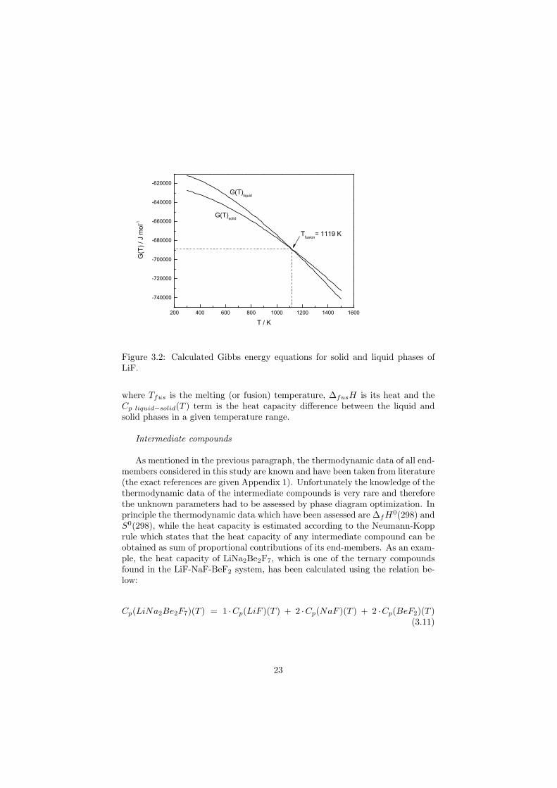
If the Equation 3.2, and Equation 3.3 are known, the thermodynamic stabil-ity of the pure compound is described. However, each relation applies only to asingle phase. In other words, if one wants to study a compound that undergoesany phase transition it is necessary to know the Gibbs energy functions of bothphases. In case of pure LiF in Figure 3.1 there are two phases considered; thesolid phase and the liquid phase. The Gibbs energy equations for both phaseshave been calculated in this study and are reported in Figure 3.2. It is evidentthat at the temperatures lower than the melting point, the Gibbs function of thesolid phase is more negative than the Gibbs energy function of the liquid phaseand the LiF crystal is stable in this region. Above this temperature the situationis opposite and the liquid phase becomes stable. At the melting temperature thetwo functions cross and are equal according to Equation 3.8. At this point thethermodynamic equilibrium between the solid and the liquid phase is achieved.

T = Tfus : G(T )solid = G(T )liquid (3.8)

∆fH0(298), S0(298) and Cp(T ) are known for most of the end-membersconsidered in this study and thus the construction of the Gibbs equations ispossible according to Equation 3.2. However it very often happens that thesesets of data are not compatible and do not reproduce the transition points (e.g.melting points) exactly. In such cases it is possible to correct the ∆fH0(298),S0(298) data of the higher temperature phase based on the knowledge of thetransition temperature and its heat in order to make a constraint at the transi-tion point. Two following equations show the calculation of ∆fH0(298), S0(298)for a liquid phase using the knowledge of the thermodynamic data of the solidphase:

∆fH0liquid(298) = ∆fH0

solid(298) + ∆fusH −

(

∫ Tfus

298

∆Cp liquid−solid(T )dT

)

(3.9)

S0liquid = S0

solid +

(

∆fusH

Tfus

)

−

(

∫ Tfus

298

(

∆Cp liquid−solid(T )

T

)

dT

)

(3.10)

22

200 400 600 800 1000 1200 1400 1600

-740000

-720000

-700000

-680000

-660000

-640000

-620000

G(T)solid

G(T

) / J m

ol-1

T / K

G(T)liquid

Tfusion

= 1119 K

Figure 3.2: Calculated Gibbs energy equations for solid and liquid phases ofLiF.

where Tfus is the melting (or fusion) temperature, ∆fusH is its heat and theCp liquid−solid(T ) term is the heat capacity difference between the liquid andsolid phases in a given temperature range.

Intermediate compounds

As mentioned in the previous paragraph, the thermodynamic data of all end-members considered in this study are known and have been taken from literature(the exact references are given Appendix 1). Unfortunately the knowledge of thethermodynamic data of the intermediate compounds is very rare and thereforethe unknown parameters had to be assessed by phase diagram optimization. Inprinciple the thermodynamic data which have been assessed are ∆fH0(298) andS0(298), while the heat capacity is estimated according to the Neumann-Kopprule which states that the heat capacity of any intermediate compound can beobtained as sum of proportional contributions of its end-members. As an exam-ple, the heat capacity of LiNa2Be2F7, which is one of the ternary compoundsfound in the LiF-NaF-BeF2 system, has been calculated using the relation be-low:

Cp(LiNa2Be2F7)(T ) = 1 ·Cp(LiF )(T ) + 2 ·Cp(NaF )(T ) + 2 ·Cp(BeF2)(T )(3.11)

23

Pure compounds - gaseous phases

Figure 3.1 shows ’only’ solid-liquid equilibria in the LiF-NaF binary system.To calculate such a diagram it is necessary to have thermodynamic data of thecondensed phases relevant to that system. However, one of the aims of thisstudy is to determine vapour pressures of the molten salt compositions whichare of interest for nuclear applications. For this reason it is required to have thethermodynamic data of the gaseous species that are formed above the solid orliquid phases. The Gibbs equations of gaseous species are calculated accordingto Equation 3.2 and the vapour pressure is calculated using the following set ofrelations (Equation 3.12- 3.16):

As an example let us assume the vaporization of the pure LiF liquid phaseinto the monomeric gaseous species as given in reaction below:

LiFliquid → LiFgas (3.12)

The difference in the Gibbs energy between the reactant and the product isdefined as:

GLiF (gas)(T ) − GLiF (liquid)(T ) = −R T ln K (3.13)

where K is the equilibrium constant of the reaction and is defined as:

K =aLiF (gas)

aLiF (liquid)(3.14)

aLiF (gas) and aLiF (liquid) in Equation 3.14 are the activities of a given speciesin the gas phase and in the liquid phase respectively. Since the activity of theliquid phase of a pure compound in equilibrium is equal to 1 and the activity ofthe gas phase is equal to its partial pressure according to Equation 3.15, wherep0 is the standard pressure and is equal to 100000 Pa (1 bar), the final relationfor the vapour pressure calculation can be written as shown in Equation 3.16.

aLiF (gas) =pLiF (gas)

p0(3.15)

pLiF (gas) = p0 exp

(

−(GLiF (gas)(T ) − GLiF (liquid)(T ))

RT

)

(3.16)

The thermodynamic data of all compounds and their phases considered inthis work are listed in Appendix 1.

Binary solutions

The definition of the Gibbs Energy function for pure compounds is shown inEquation 3.2. In case of the binary solutions the Gibbs function is defined byEquation 3.17 as a weighted average of Gibbs energies of the pure componentsthat the solution consists of plus the mixing contribution of these end-members.

24

G(T ) = x1G1(T ) + x2G2(T ) + Gmixing(T ) (3.17)

The mixing contribution is basically distinguished into two parts, the ideal mix-ing contribution which is related to the configurational entropy and is definedas

Gideal mixing(T ) = x1RTlnx1 + x2RTlnx2 (3.18)

and the excess Gibbs contribution which is typical for the real systems (systemwithout any excess contributions are referred to as ideal systems). CombiningEquations 3.17 and 3.18 the total Gibbs function of a solution can be writtenas:

G(T ) = x1G1(T ) + x2G2(T ) + x1RTlnx1 + x2RTlnx2 + Gexcess (3.19)

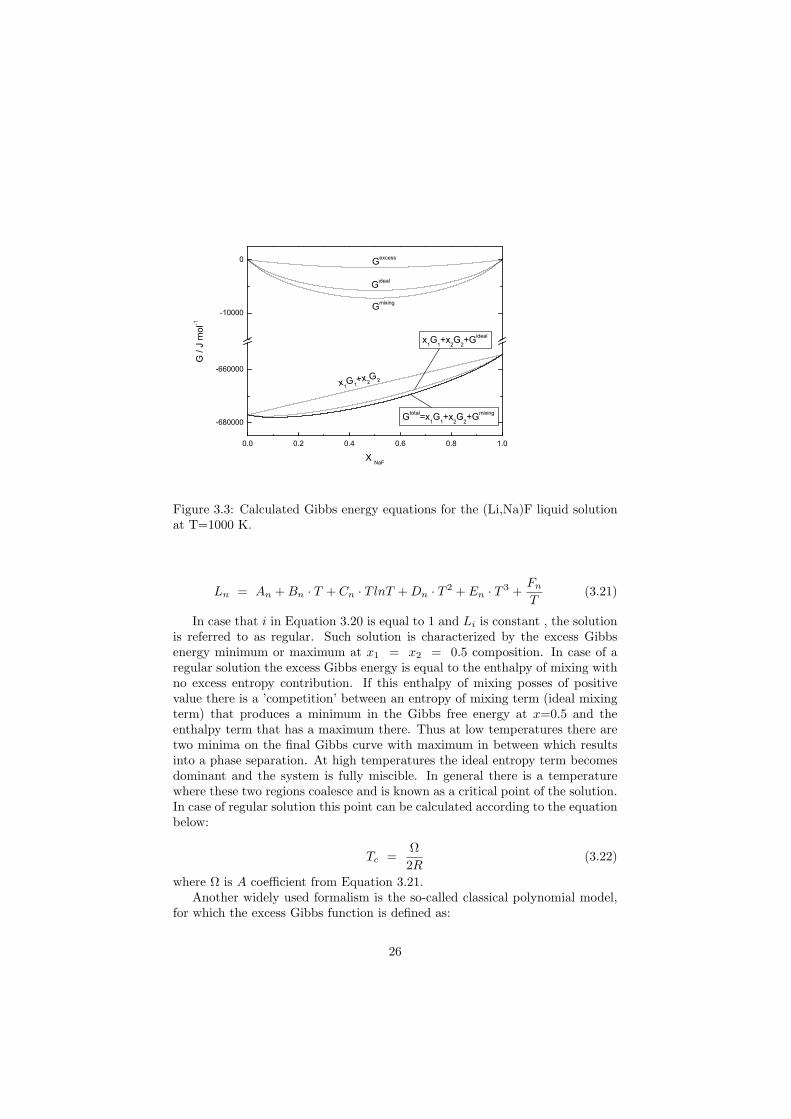
Figure 3.3 shows the influence of the various contributions to the totalGibbs function, demonstrated for the (Li,Na)F liquid solution calculated forT = 1000 K. The graph is divided into two parts. In the upper part the ’small’energy contributions, the mixing energies are showed. Since the mixing occursonly in the region between the end-members these mixing contribution (ideal orexcess) are always zero at the end-member compositions. In the lower part ofthe diagram a comparison between the the linear x1G1(T )+x2G2(T ) term fromEquation 3.17, the Gibbs function of the ideal solution (Equation 3.18) and theGibbs function of the real solution is depicted. The last curve corresponds tothe total Gibbs energy of the (Li,Na)F liquid solution and is highlighted by abold line.

It is important to note that in case the solution is not created between theend-members (e.g. the solid region in the LiF-PuF3 simple eutectic systemshown in Figure 5.13) logically there are no mixing contributions and the to-tal Gibbs energy of any composition of such two-phase system is equal to thex1G1(T ) + x2G2(T ) term.

Thermodynamic models for the excess Gibbs parametersof the binary solutions

Since it is very difficult to experimentally determine the excess Gibbs propertiesof the solutions, the optimization of these data is usually the main task in orderto assess phase diagrams. There are several thermodynamic models developedfor this purpose. Probably the most common is the Redlich-Kister model whichis defined as:

Gexcess = x1 · x2 ·∑

i=n

(x1 − x2)i−1 · Li (3.20)

which is a function of the mole fractions (x1 and x2) and the excess Gibbsenergy coefficients (Li) that are in a polynomial form and can be a function oftemperature as given below:

25

0.0 0.2 0.4 0.6 0.8 1.0

-680000

-660000

-10000

0

x1G

1+x

2G

2+G

ideal

Gmixing

Gideal

G / J

mo

l-1

X NaF

Gexcess

x1G1

+x2G2

Gtotal

=x1G

1+x

2G

2+G

mixing

Figure 3.3: Calculated Gibbs energy equations for the (Li,Na)F liquid solutionat T=1000 K.

Ln = An + Bn · T + Cn · T lnT + Dn · T2 + En · T

3 +Fn

T(3.21)

In case that i in Equation 3.20 is equal to 1 and Li is constant , the solutionis referred to as regular. Such solution is characterized by the excess Gibbsenergy minimum or maximum at x1 = x2 = 0.5 composition. In case of aregular solution the excess Gibbs energy is equal to the enthalpy of mixing withno excess entropy contribution. If this enthalpy of mixing posses of positivevalue there is a ’competition’ between an entropy of mixing term (ideal mixingterm) that produces a minimum in the Gibbs free energy at x=0.5 and theenthalpy term that has a maximum there. Thus at low temperatures there aretwo minima on the final Gibbs curve with maximum in between which resultsinto a phase separation. At high temperatures the ideal entropy term becomesdominant and the system is fully miscible. In general there is a temperaturewhere these two regions coalesce and is known as a critical point of the solution.In case of regular solution this point can be calculated according to the equationbelow:

Tc =Ω

2R(3.22)

where Ω is A coefficient from Equation 3.21.Another widely used formalism is the so-called classical polynomial model,

for which the excess Gibbs function is defined as:

26

Gexcess =n∑

i,j=1

Xi1 ·X

j2 · Lij (3.23)

where Lij are the excess Gibbs energy parameters to be optimized and are ina polynomial form similarly to Equation 3.21. In this study this model hasbeen used to assess the excess properties of all solid solutions and for the liquiddescription of the LiF-BeF2-ZrF4-UF4 system. The obtained coefficient for bothsolutions are listed in Appendix 2.

In case of the NaF-RbF, NaF-CsF, LiF-KF, LiF-RbF and LiF-CsF binarysystems, there is no solid solubility reported. However in order to keep thethermodynamic data of the (Li,Na,K,Rb,Cs)F solid solution complete and toextrapolate this solution into higher order field (ternary, quaternary systemsetc.), these binary solutions had to be treated as systems with totally immisci-ble solid solubility. This was done by introducing relatively big arbitrary excessGibbs terms as shown in Appendix 2.

Modified Quasi-Chemical model

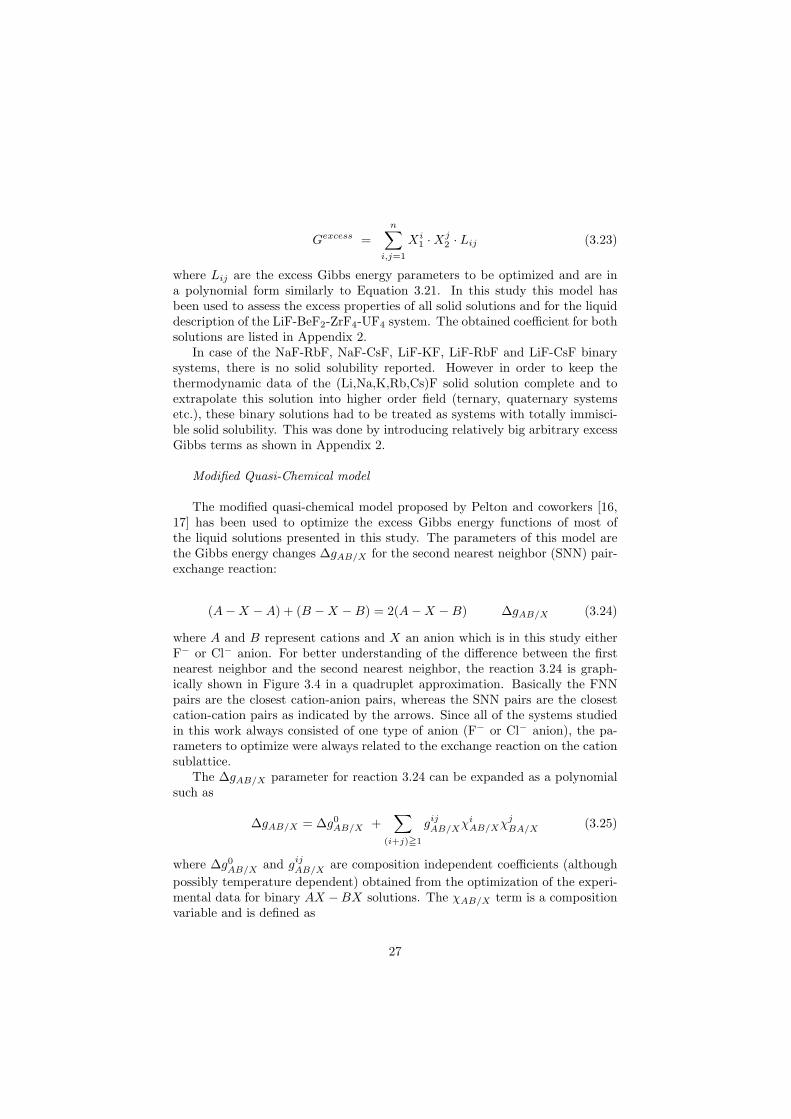
The modified quasi-chemical model proposed by Pelton and coworkers [16,17] has been used to optimize the excess Gibbs energy functions of most ofthe liquid solutions presented in this study. The parameters of this model arethe Gibbs energy changes ∆gAB/X for the second nearest neighbor (SNN) pair-exchange reaction:

(A−X −A) + (B −X −B) = 2(A−X −B) ∆gAB/X (3.24)

where A and B represent cations and X an anion which is in this study eitherF− or Cl− anion. For better understanding of the difference between the firstnearest neighbor and the second nearest neighbor, the reaction 3.24 is graph-ically shown in Figure 3.4 in a quadruplet approximation. Basically the FNNpairs are the closest cation-anion pairs, whereas the SNN pairs are the closestcation-cation pairs as indicated by the arrows. Since all of the systems studiedin this work always consisted of one type of anion (F− or Cl− anion), the pa-rameters to optimize were always related to the exchange reaction on the cationsublattice.

The ∆gAB/X parameter for reaction 3.24 can be expanded as a polynomialsuch as

∆gAB/X = ∆g0AB/X +

∑

(i+j)≧1

gijAB/Xχi

AB/XχjBA/X (3.25)

where ∆g0AB/X and gij

AB/X are composition independent coefficients (although

possibly temperature dependent) obtained from the optimization of the experi-mental data for binary AX −BX solutions. The χAB/X term is a compositionvariable and is defined as

27

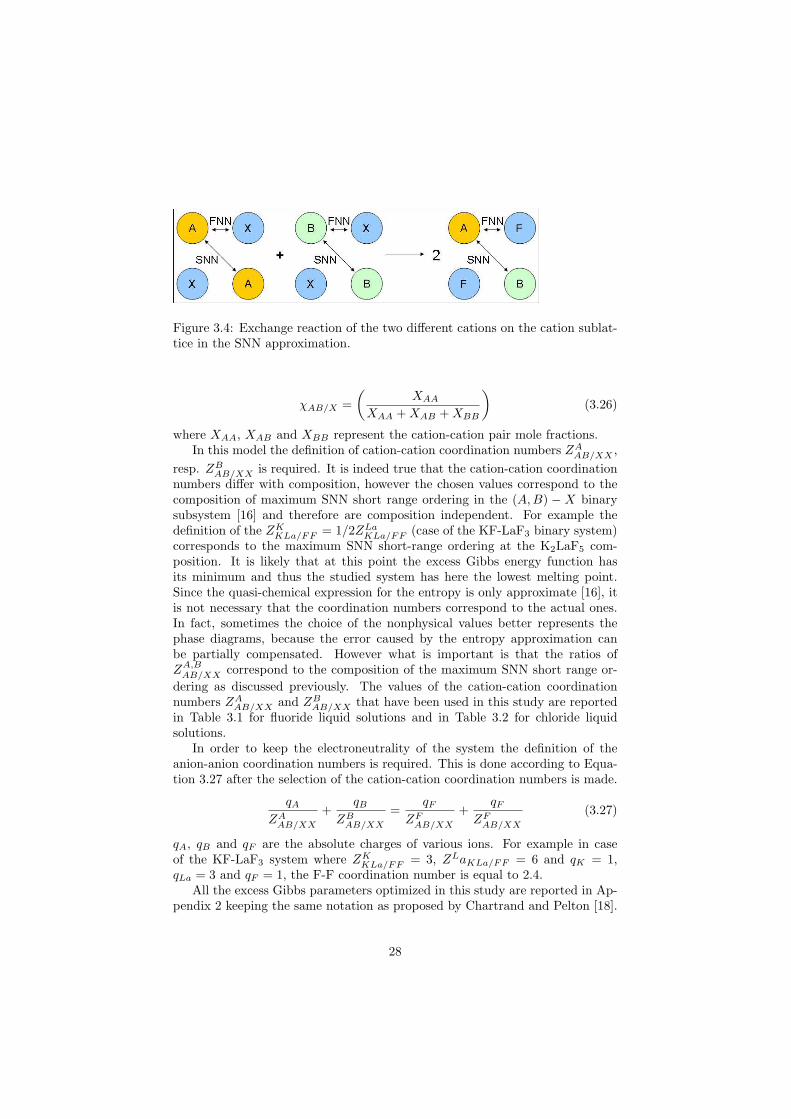
Figure 3.4: Exchange reaction of the two different cations on the cation sublat-tice in the SNN approximation.

χAB/X =

(

XAA

XAA + XAB + XBB

)

(3.26)

where XAA, XAB and XBB represent the cation-cation pair mole fractions.In this model the definition of cation-cation coordination numbers ZA

AB/XX ,

resp. ZBAB/XX is required. It is indeed true that the cation-cation coordination

numbers differ with composition, however the chosen values correspond to thecomposition of maximum SNN short range ordering in the (A, B) − X binarysubsystem [16] and therefore are composition independent. For example thedefinition of the ZK

KLa/FF = 1/2ZLaKLa/FF (case of the KF-LaF3 binary system)

corresponds to the maximum SNN short-range ordering at the K2LaF5 com-position. It is likely that at this point the excess Gibbs energy function hasits minimum and thus the studied system has here the lowest melting point.Since the quasi-chemical expression for the entropy is only approximate [16], itis not necessary that the coordination numbers correspond to the actual ones.In fact, sometimes the choice of the nonphysical values better represents thephase diagrams, because the error caused by the entropy approximation canbe partially compensated. However what is important is that the ratios ofZA,B

AB/XX correspond to the composition of the maximum SNN short range or-

dering as discussed previously. The values of the cation-cation coordinationnumbers ZA

AB/XX and ZBAB/XX that have been used in this study are reported

in Table 3.1 for fluoride liquid solutions and in Table 3.2 for chloride liquidsolutions.

In order to keep the electroneutrality of the system the definition of theanion-anion coordination numbers is required. This is done according to Equa-tion 3.27 after the selection of the cation-cation coordination numbers is made.

qA

ZAAB/XX

+qB

ZBAB/XX

=qF

ZFAB/XX

+qF

ZFAB/XX

(3.27)

qA, qB and qF are the absolute charges of various ions. For example in caseof the KF-LaF3 system where ZK

KLa/FF = 3, ZLaKLa/FF = 6 and qK = 1,qLa = 3 and qF = 1, the F-F coordination number is equal to 2.4.

All the excess Gibbs parameters optimized in this study are reported in Ap-pendix 2 keeping the same notation as proposed by Chartrand and Pelton [18].

28

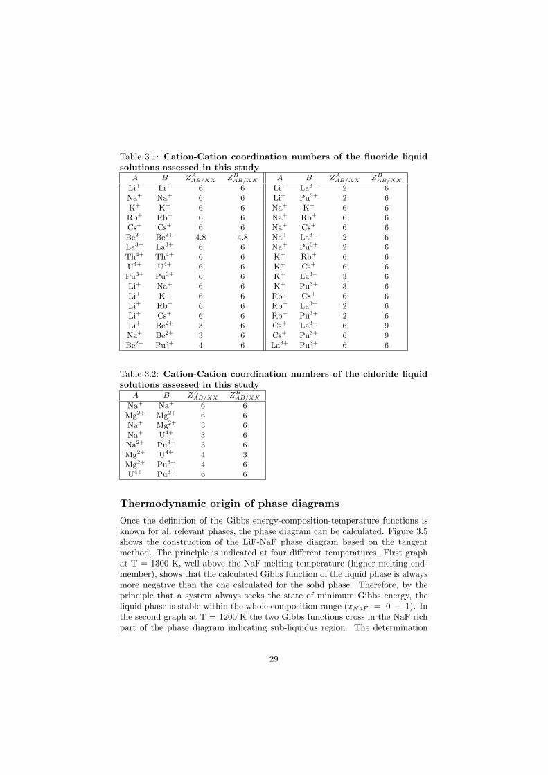
Table 3.1: Cation-Cation coordination numbers of the fluoride liquidsolutions assessed in this study

A B ZAAB/XX ZB

AB/XX A B ZAAB/XX ZB

AB/XX

Li+ Li+ 6 6 Li+ La3+ 2 6Na+ Na+ 6 6 Li+ Pu3+ 2 6K+ K+ 6 6 Na+ K+ 6 6Rb+ Rb+ 6 6 Na+ Rb+ 6 6Cs+ Cs+ 6 6 Na+ Cs+ 6 6Be2+ Be2+ 4.8 4.8 Na+ La3+ 2 6La3+ La3+ 6 6 Na+ Pu3+ 2 6Th4+ Th4+ 6 6 K+ Rb+ 6 6U4+ U4+ 6 6 K+ Cs+ 6 6Pu3+ Pu3+ 6 6 K+ La3+ 3 6Li+ Na+ 6 6 K+ Pu3+ 3 6Li+ K+ 6 6 Rb+ Cs+ 6 6Li+ Rb+ 6 6 Rb+ La3+ 2 6Li+ Cs+ 6 6 Rb+ Pu3+ 2 6Li+ Be2+ 3 6 Cs+ La3+ 6 9Na+ Be2+ 3 6 Cs+ Pu3+ 6 9Be2+ Pu3+ 4 6 La3+ Pu3+ 6 6

Table 3.2: Cation-Cation coordination numbers of the chloride liquidsolutions assessed in this study

A B ZAAB/XX ZB

AB/XX

Na+ Na+ 6 6Mg2+ Mg2+ 6 6Na+ Mg2+ 3 6Na+ U4+ 3 6Na2+ Pu3+ 3 6Mg2+ U4+ 4 3Mg2+ Pu3+ 4 6U4+ Pu3+ 6 6

Thermodynamic origin of phase diagrams

Once the definition of the Gibbs energy-composition-temperature functions isknown for all relevant phases, the phase diagram can be calculated. Figure 3.5shows the construction of the LiF-NaF phase diagram based on the tangentmethod. The principle is indicated at four different temperatures. First graphat T = 1300 K, well above the NaF melting temperature (higher melting end-member), shows that the calculated Gibbs function of the liquid phase is alwaysmore negative than the one calculated for the solid phase. Therefore, by theprinciple that a system always seeks the state of minimum Gibbs energy, theliquid phase is stable within the whole composition range (xNaF = 0 − 1). Inthe second graph at T = 1200 K the two Gibbs functions cross in the NaF richpart of the phase diagram indicating sub-liquidus region. The determination

29

of the liquidus and solidus points is made by tangent method as shown in thefigure. P1 and Q1 are two points, where the tangent line (red line) touchesthe Gibbs functions of the liquid and solid phases, and correspond respectivelyto the liquidus and solidus point from the LiF-NaF phase diagram (very bot-tom graph in Figure 3.5). Third graph shows the Gibbs functions calculated atT = 1050 K. As it is seen from the figure, there are two intersections betweenthe two Gibbs functions. Therefore two tangent lines are constructed in orderto obtain two liquidus and two solidus points indicated by Q2, P ′2 and P2, Q′2points respectively. The last graph has been calculated for T = 800 K and showsthat the Gibbs energy function of the solid phase is more negative than the onefor the liquid phase. It thus indicates the sub-solidus region, meaning that noliquid phase is in equilibrium within the whole composition range. Howeverthere is a tangential line plotted on the Gibbs function of the solid phase. Thisis because there are two inflections on the Gibbs curve (it is not very obviousfrom the figure since the curvature is very broad, but the detailed calculationconfirms the inflections) indicating a miscibility gap of the solid solution. Thecompositions of the solid solution that are in equilibrium are indicated by theP3 and Q3 points.

Higher order systems approximations

After the binary phase diagram are assessed, the higher order systems can beextrapolated based on the knowledge of the binary excess Gibbs energy data.The way of extrapolating the higher order systems is a very important tool,because it is very difficult and time consuming to measure every ternary (orhigher) system. Already among the 10 fluorides considered in this study 120ternary (10!/3!·7!) and 210 (10!/4!·6!) quaternary systems are formed. Takinginto account the fact how many measurements are necessary in order to preciselydescribe even a very simple ternary phase diagram, the way of extrapolatingthese systems is sometimes the only possible choice.

There are several formalisms proposed, among which the Muggianu, Kohlerand Kohler/Toop formalism are most widely used. The first two are symmet-ric, whereas the Kohler/Toop formalism is asymmetric where one of the end-members is singled out. The use of a symmetric model in case an asymmetricmodel is more appropriate can give rise to errors. Graphical schemes of theexcess Gibbs energy approximation for a single ternary composition using threementioned approaches is shown in Figure 3.6.

As illustrated in the figure, the excess Gibbs energy of the ternary com-position ’x’ is calculated as a contribution of the excess Gibbs energies of the’p’, ’q’ and ’r’ compositions from the A-B, A-C and B-C binary subsystemsrespectivelly.

In this study two groups of symmetry have been established. The first oneconsisted of LiF, NaF, KF, RbF and CsF compounds in case of the fluoridesand NaCl in case of chloride systems, whereas BeF2, LaF3, ZrF4, UF4 and PuF3

compounds in case of fluorides and MgCl2, UCl3 and PuCl3 compounds from

30

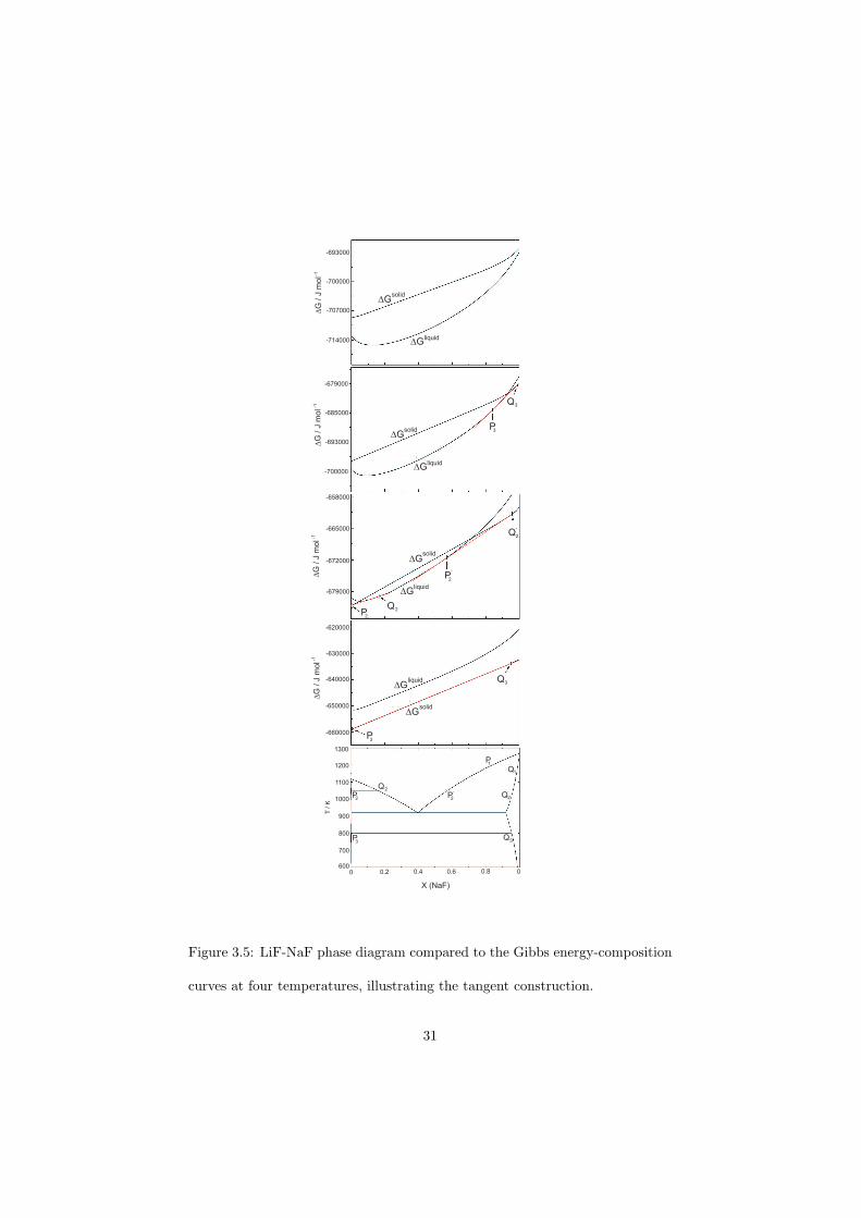
solid

∆G

∆G

liquid

2

`P

QP

2

2

Q

Q`2

∆G

/ J

mol-1

-658000

-665000

-672000

-679000

∆Gliquid

∆Gsolid

Q3

3P

-620000

-630000

-640000

-650000

-660000

∆G

/ J

mol-1

∆G

/ J

mol-1

∆G

∆G

solid

liquid

Q

P3

3

-679000

-700000

-693000

-685000

∆Gsolid

∆Gliquid

∆G

/ J

mo

l

-693000

-700000

-707000

-714000

-1

1300

1200

1100

1000

900

800

700

600

T / K

0 0.40.2 0.6 0.8 0

PQ

QP

P

P

Q

Q

1

1

2

2

22` `

33

X (NaF)

Figure 3.5: LiF-NaF phase diagram compared to the Gibbs energy-composition

curves at four temperatures, illustrating the tangent construction.

31

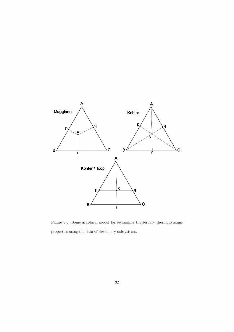
Figure 3.6: Some graphical model for estimating the ternary thermodynamic

properties using the data of the binary subsystems.

32

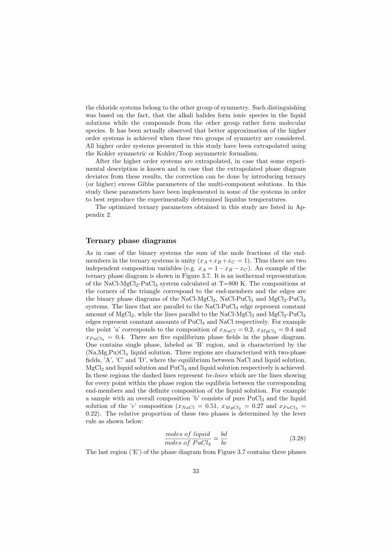
the chloride systems belong to the other group of symmetry. Such distinguishingwas based on the fact, that the alkali halides form ionic species in the liquidsolutions while the compounds from the other group rather form molecularspecies. It has been actually observed that better approximation of the higherorder systems is achieved when these two groups of symmetry are considered.All higher order systems presented in this study have been extrapolated usingthe Kohler symmetric or Kohler/Toop asymmetric formalism.

After the higher order systems are extrapolated, in case that some experi-mental description is known and in case that the extrapolated phase diagramdeviates from these results, the correction can be done by introducing ternary(or higher) excess Gibbs parameters of the multi-component solutions. In thisstudy these parameters have been implemented in some of the systems in orderto best reproduce the experimentally determined liquidus temperatures.

The optimized ternary parameters obtained in this study are listed in Ap-pendix 2.

Ternary phase diagrams

As in case of the binary systems the sum of the mole fractions of the end-members in the ternary systems is unity (xA+xB +xC = 1). Thus there are twoindependent composition variables (e.g. xA = 1−xB −xC). An example of theternary phase diagram is shown in Figure 3.7. It is an isothermal representationof the NaCl-MgCl2-PuCl3 system calculated at T=800 K. The compositions atthe corners of the triangle correspond to the end-members and the edges arethe binary phase diagrams of the NaCl-MgCl2, NaCl-PuCl3 and MgCl2-PuCl3systems. The lines that are parallel to the NaCl-PuCl3 edge represent constantamount of MgCl2, while the lines parallel to the NaCl-MgCl2 and MgCl2-PuCl3edges represent constant amounts of PuCl3 and NaCl respectively. For examplethe point ’a’ corresponds to the composition of xNaCl = 0.2, xMgCl2 = 0.4 andxPuCl3 = 0.4. There are five equilibrium phase fields in the phase diagram.One contains single phase, labeled as ’B’ region, and is characterized by the(Na,Mg,Pu)Clx liquid solution. Three regions are characterized with two-phasefields, ’A’, ’C’ and ’D’, where the equilibrium between NaCl and liquid solution,MgCl2 and liquid solution and PuCl3 and liquid solution respectively is achieved.In these regions the dashed lines represent tie-lines which are the lines showingfor every point within the phase region the equlibria between the correspondingend-members and the definite composition of the liquid solution. For examplea sample with an overall composition ’b’ consists of pure PuCl3 and the liquidsolution of the ’c’ composition (xNaCl = 0.51, xMgCl2 = 0.27 and xPuCl3 =0.22). The relative proportion of these two phases is determined by the leverrule as shown below:

moles of liquid

moles of PuCl3=

bd

bc(3.28)

The last region (’E’) of the phase diagram from Figure 3.7 contains three phases

33

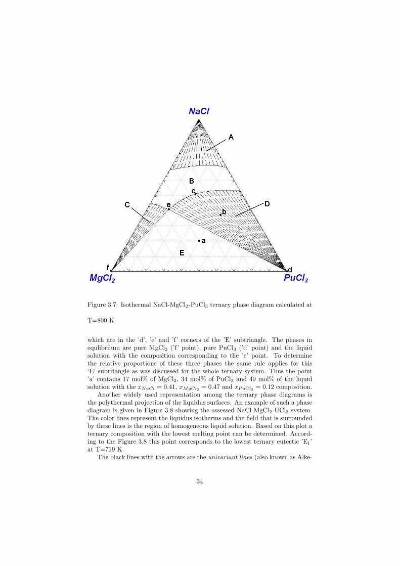
Figure 3.7: Isothermal NaCl-MgCl2-PuCl3 ternary phase diagram calculated at

T=800 K.

which are in the ’d’, ’e’ and ’f’ corners of the ’E’ subtriangle. The phases inequlibriium are pure MgCl2 (’f’ point), pure PuCl3 (’d’ point) and the liquidsolution with the composition corresponding to the ’e’ point. To determinethe relative proportions of these three phases the same rule applies for this’E’ subtriangle as was discussed for the whole ternary system. Thus the point’a’ contains 17 mol% of MgCl2, 34 mol% of PuCl3 and 49 mol% of the liquidsolution with the xNaCl = 0.41, xMgCl2 = 0.47 and xPuCl3 = 0.12 composition.

Another widely used representation among the ternary phase diagrams isthe polythermal projection of the liquidus surfaces. An example of such a phasediagram is given in Figure 3.8 showing the assessed NaCl-MgCl2-UCl3 system.The color lines represent the liquidus isotherms and the field that is surroundedby these lines is the region of homogeneous liquid solution. Based on this plot aternary composition with the lowest melting point can be determined. Accord-ing to the Figure 3.8 this point corresponds to the lowest ternary eutectic ’E1’at T=719 K.

The black lines with the arrows are the univariant lines (also known as Alke-

34

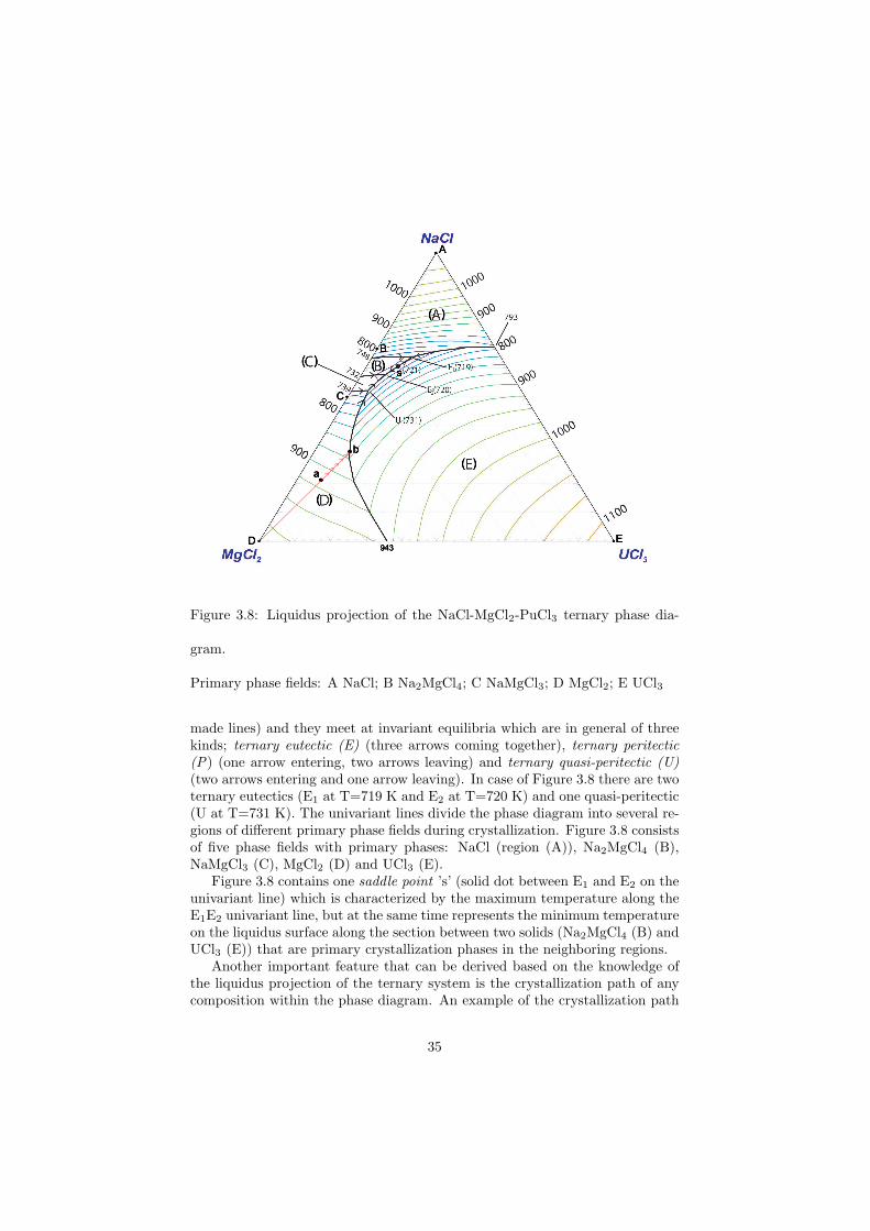
Figure 3.8: Liquidus projection of the NaCl-MgCl2-PuCl3 ternary phase dia-

gram.

Primary phase fields: A NaCl; B Na2MgCl4; C NaMgCl3; D MgCl2; E UCl3

made lines) and they meet at invariant equilibria which are in general of threekinds; ternary eutectic (E) (three arrows coming together), ternary peritectic(P) (one arrow entering, two arrows leaving) and ternary quasi-peritectic (U)(two arrows entering and one arrow leaving). In case of Figure 3.8 there are twoternary eutectics (E1 at T=719 K and E2 at T=720 K) and one quasi-peritectic(U at T=731 K). The univariant lines divide the phase diagram into several re-gions of different primary phase fields during crystallization. Figure 3.8 consistsof five phase fields with primary phases: NaCl (region (A)), Na2MgCl4 (B),NaMgCl3 (C), MgCl2 (D) and UCl3 (E).

Figure 3.8 contains one saddle point ’s’ (solid dot between E1 and E2 on theunivariant line) which is characterized by the maximum temperature along theE1E2 univariant line, but at the same time represents the minimum temperatureon the liquidus surface along the section between two solids (Na2MgCl4 (B) andUCl3 (E)) that are primary crystallization phases in the neighboring regions.

Another important feature that can be derived based on the knowledge ofthe liquidus projection of the ternary system is the crystallization path of anycomposition within the phase diagram. An example of the crystallization path

35

determination is shown in Figure 3.8. Let us consider the initial compositionof the liquid solution represented by point ’a’ (xNaCl = 0.21, xMgCl2 = 0.72and xUCl3 = 0.07). Since this point belongs to the primary phase field ofMgCl2, this compound will also be the first solid to precipitate upon the coolingand according to the phase diagram the first crystal will appear at T=916 K(between the 900 K and 925 K isotherm). During further cooling the liquid phasebecomes depleted in MgCl2, but the ratio NaCl/UCl3 in the liquid remainsconstant. Therefore the crystallization path in this temperature range is astraight line (red line with arrows in Figure 3.8) passing through the MgCl2end-member and the initial composition ’a’. It must be noted that in case thata solid solution rather than the pure compound is formed, the crystallizationpath would not be a straight line in this region.

When the composition of the liquid reaches the univariant line in point ’b’at T=867 K the UCl3 compound starts to precipitate. At this point the relativeproportions of solid MgCl2 and the liquid solution is defined by the lever ruleon the ’Dab’ tie-line according to:

moles of liquid

moles of MgCl2=

Da

ab(3.29)

Upon further cooling the crystallization path continues along the univariantline towards the first invariant equlibria at T=731 K, the quasi-peritectic (U),while two solids (MgCl2 and UCl3) co-precipitate as a binary mixture. At thispoint the quasi-peritectic reaction occurs:

L + MgCl2(D − phase) = UCl3(E − phase) + NaMgCl3(C − phase) (3.30)

Since there are two reactants in the reaction above, two possibilities can occur.In the first case the liquid is completely consumed before the MgCl2 phase andthe solidification will finish at this point. Another option is that the MgCl2phase is consumed prior to the liquid and the solidification continues alongthe ’UE2’ univariant line towards the ternary eutectic (E2) at T=720 K, whileco-precipitation of the UCl3 (E-phase) and NaMgCl3 (C-phase) phases. Atthis point the liquid solution would solidify eutectically according to followingequation:

L = UCl3(E−phase)+NaMgCl3(C−phase)+Na2MgCl4(B−phase) (3.31)

To determine which situation will occur the mass balance criterion is appliedthat states that for a three phase equilibrium, the overall composition (’a’ point)must always lie within the tie-triangle formed by the compositions of the threephases [19]. The tie-triangle joining the C,D and E phases contains the ’a’composition, whereas the other tie-triangle joining the phases E and C and theliquid at U does not. Hence the first situation will happen and the solidificationof the ’a’ composition is finished at ternary quasi-peritectic (U).

36

It must be noted that in case of the ternary peritectic (P-type transition) (notthe case in Figure 3.8) the following general reaction occurs:

L + α + β = γ (3.32)

Since there are three reactants, also three different events can take place. Ei-ther the liquid is consumed prior to α and β phases, that the solidification endat this point. Or α phase is consumed as the first phase, then the crystalliza-tion continues along the invariant line with the co-precipitation of the β and γphases or the β phase is consumed prior to the liquid and the α phase and thecrystallization continues along the invariant line with the co-precipitation of theα and γ phases. Which one of these three situations occurs is defined by thetie-triangles as discussed in the paragraph above.

37

Chapter 4

Thermodynamic data

It has been demonstrated in the previous section that in order to calculatethe phase diagram the knowledge of the thermodynamic data of all containedphases is necessary. These data can be determined either experimentally or op-timized during the thermodynamic assessment. However even the optimizationis principally based on the experimental data and therefore the measurementsare always the basis of any thermodynamic description. Beside the experimentalapproach another way how to obtain the thermodynamic data are the first prin-ciple calculations. This method is nowadays more and more applied, especiallyin the nuclear research where the laboratory work is limited due to the handlingrisks of radioactive materials. However also here it is useful to correlate theseresults with the experiment.

In this part of the work various techniques that have been used to study thefluoride systems will be presented and the results of the measurements will bereported. A special section is dedicated for the description of the new encap-sulation technique which has been developed within the frame of this thesis inorder to measure the fluoride samples to high temperatures (T > 1273 K). Thechapter is divided into three main sections. In the first one the calorimetricstudies used for the heat capacity determination are introduced while in thesecond part the thermal analysis used to acquire the equilibrium data (phasetransitions, solidus, liquidus) is discussed. In the last part the ab initio approachis demonstrated on the RbF-CsF system for which the excess properties of the(Rb,Cs)F solid solution have been calculated and the results have been used toassess the RbF-CsF phase diagram.

38

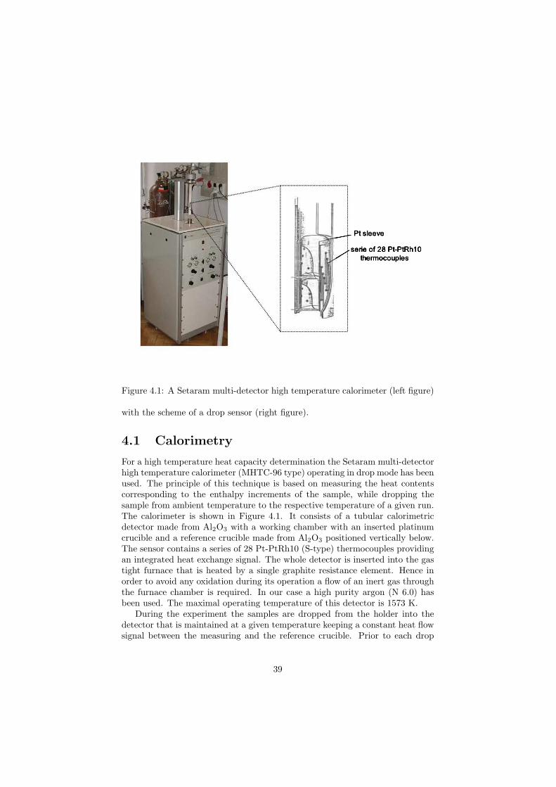
Figure 4.1: A Setaram multi-detector high temperature calorimeter (left figure)

with the scheme of a drop sensor (right figure).

4.1 Calorimetry

For a high temperature heat capacity determination the Setaram multi-detectorhigh temperature calorimeter (MHTC-96 type) operating in drop mode has beenused. The principle of this technique is based on measuring the heat contentscorresponding to the enthalpy increments of the sample, while dropping thesample from ambient temperature to the respective temperature of a given run.The calorimeter is shown in Figure 4.1. It consists of a tubular calorimetricdetector made from Al2O3 with a working chamber with an inserted platinumcrucible and a reference crucible made from Al2O3 positioned vertically below.The sensor contains a series of 28 Pt-PtRh10 (S-type) thermocouples providingan integrated heat exchange signal. The whole detector is inserted into the gastight furnace that is heated by a single graphite resistance element. Hence inorder to avoid any oxidation during its operation a flow of an inert gas throughthe furnace chamber is required. In our case a high purity argon (N 6.0) hasbeen used. The maximal operating temperature of this detector is 1573 K.

During the experiment the samples are dropped from the holder into thedetector that is maintained at a given temperature keeping a constant heat flowsignal between the measuring and the reference crucible. Prior to each drop

39

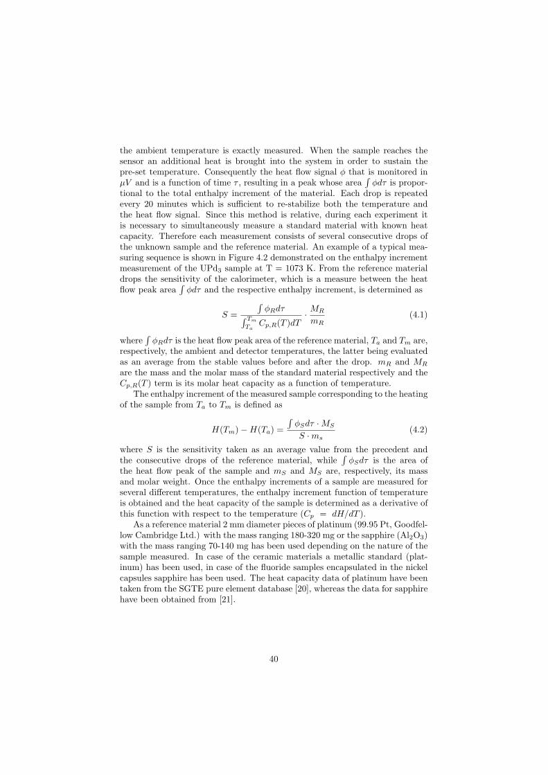
the ambient temperature is exactly measured. When the sample reaches thesensor an additional heat is brought into the system in order to sustain thepre-set temperature. Consequently the heat flow signal φ that is monitored inµV and is a function of time τ , resulting in a peak whose area

∫

φdτ is propor-tional to the total enthalpy increment of the material. Each drop is repeatedevery 20 minutes which is sufficient to re-stabilize both the temperature andthe heat flow signal. Since this method is relative, during each experiment itis necessary to simultaneously measure a standard material with known heatcapacity. Therefore each measurement consists of several consecutive drops ofthe unknown sample and the reference material. An example of a typical mea-suring sequence is shown in Figure 4.2 demonstrated on the enthalpy incrementmeasurement of the UPd3 sample at T = 1073 K. From the reference materialdrops the sensitivity of the calorimeter, which is a measure between the heatflow peak area

∫

φdτ and the respective enthalpy increment, is determined as

S =

∫

φRdτ∫ Tm

TaCp,R(T )dT

·MR

mR(4.1)

where∫

φRdτ is the heat flow peak area of the reference material, Ta and Tm are,respectively, the ambient and detector temperatures, the latter being evaluatedas an average from the stable values before and after the drop. mR and MR

are the mass and the molar mass of the standard material respectively and theCp,R(T ) term is its molar heat capacity as a function of temperature.

The enthalpy increment of the measured sample corresponding to the heatingof the sample from Ta to Tm is defined as

H(Tm)−H(Ta) =

∫

φSdτ ·MS

S ·ms(4.2)

where S is the sensitivity taken as an average value from the precedent andthe consecutive drops of the reference material, while

∫

φSdτ is the area ofthe heat flow peak of the sample and mS and MS are, respectively, its massand molar weight. Once the enthalpy increments of a sample are measured forseveral different temperatures, the enthalpy increment function of temperatureis obtained and the heat capacity of the sample is determined as a derivative ofthis function with respect to the temperature (Cp = dH/dT ).

As a reference material 2 mm diameter pieces of platinum (99.95 Pt, Goodfel-low Cambridge Ltd.) with the mass ranging 180-320 mg or the sapphire (Al2O3)with the mass ranging 70-140 mg has been used depending on the nature of thesample measured. In case of the ceramic materials a metallic standard (plat-inum) has been used, in case of the fluoride samples encapsulated in the nickelcapsules sapphire has been used. The heat capacity data of platinum have beentaken from the SGTE pure element database [20], whereas the data for sapphirehave been obtained from [21].

40

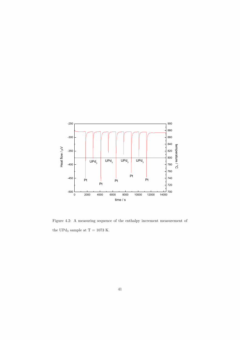
0 2000 4000 6000 8000 10000 12000 14000-500

-450

-400

-350

-300

-250

700

720

740

760

780

800

820

840

860

880

900

µ

time / s

UPd3

UPd3

UPd3

PtPt

Pt

Pt

Pt

UPd3

Figure 4.2: A measuring sequence of the enthalpy increment measurement of

the UPd3 sample at T = 1073 K.

41

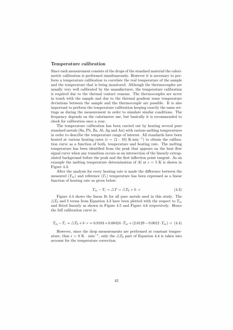
Temperature calibration

Since each measurement consists of the drops of the standard material the calori-metric calibration is performed simultaneously. However it is necessary to per-form a temperature calibration to correlate the real temperature of the sampleand the temperature that is being monitored. Although the thermocouples areusually very well calibrated by the manufacturer, the temperature calibrationis required due to the thermal contact reasons. The thermocouples are neverin touch with the sample and due to the thermal gradient some temperaturedeviations between the sample and the thermocouple are possible. It is alsoimportant to perform the temperature calibration keeping exactly the same set-tings as during the measurement in order to simulate similar conditions. Thefrequency depends on the calorimeter use, but basically it is recommended tocheck for calibration once a year.

The temperature calibration has been carried out by heating several purestandard metals (Sn, Pb, Zn, Al, Ag and Au) with various melting temperaturesin order to describe the temperature range of interest. All standards have beenheated at various heating rates (r = (2 - 10) K·min−1) to obtain the calibra-tion curve as a function of both, temperature and heating rate. The meltingtemperature has been identified from the peak that appears on the heat flowsignal curve when any transition occurs as an intersection of the linearly extrap-olated background before the peak and the first inflection point tangent. As anexample the melting temperature determination of Al at r = 5 K is shown inFigure 4.3.

After the analysis for every heating rate is made the difference between themeasured (Tm) and reference (Tr) temperature has been expressed as a linearfunction of heating rate as given below:

Tm − Tr = T = T0 + b · r (4.3)

Figure 4.4 shows the linear fit for all pure metals used in this study. TheT0 and b terms from Equation 4.3 have been plotted with the respect to Tm

and fitted linearly as shown in Figure 4.5 and Figure 4.6 respectively. Hencethe full calibration curve is:

Tm−Tr = T0 + b · r = 0.9183 + 0.00424 ·Tm + (2.6129− 0.0012 ·Tm) · r (4.4)

However, since the drop measurements are performed at constant temper-ature, thus r = 0 K · min−1, only the T0 part of Equation 4.4 is taken intoaccount for the temperature correction.

42

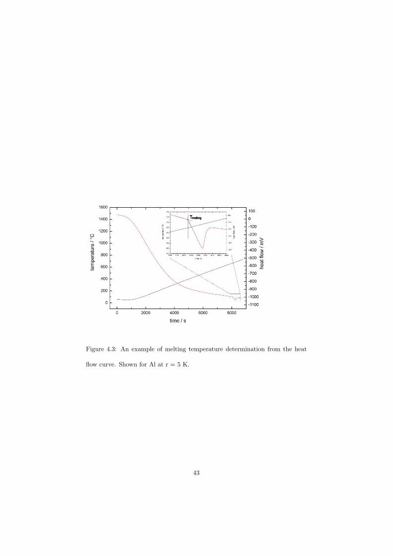
Figure 4.3: An example of melting temperature determination from the heat

flow curve. Shown for Al at r = 5 K.

43

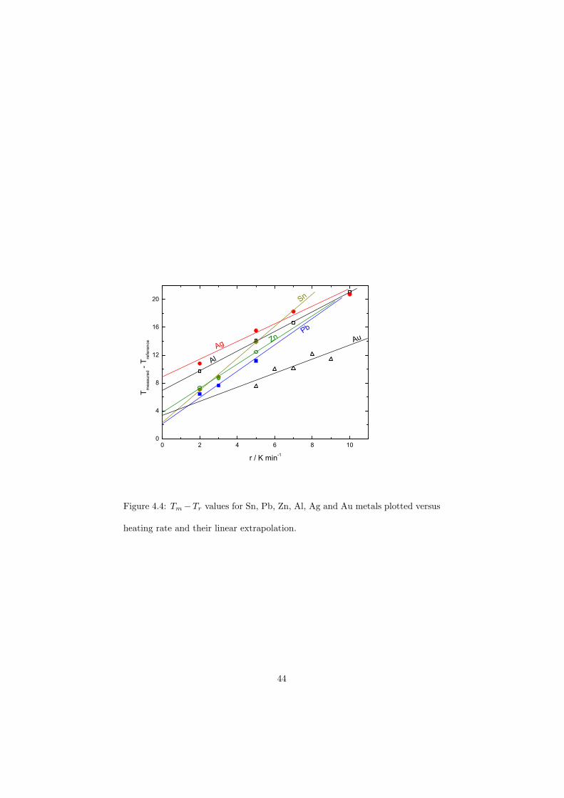
0 2 4 6 8 100

4

8

12

16

20

Tm

ea

su

red -

Tre

fere

nce

r / K min-1

AuAg

Pb

Zn

Al

Sn

Figure 4.4: Tm−Tr values for Sn, Pb, Zn, Al, Ag and Au metals plotted versus

heating rate and their linear extrapolation.

44

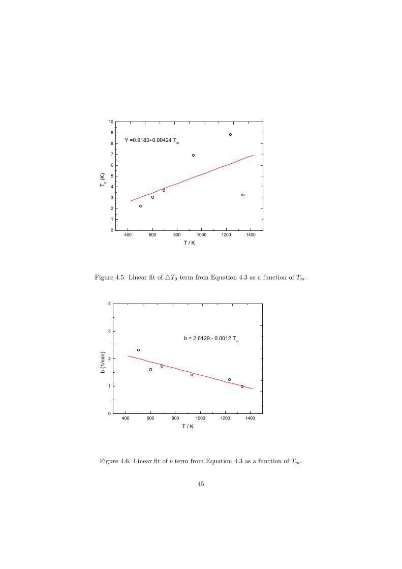
400 600 800 1000 1200 14000

1

2

3

4

5

6

7

8

9

10

Y =0.9183+0.00424 Tm

T0 (

K)

T / K

Figure 4.5: Linear fit of T0 term from Equation 4.3 as a function of Tm.

400 600 800 1000 1200 14000

1

2

3

4

b (

1/m

in)

T / K

b = 2.6129 - 0.0012 Tm

Figure 4.6: Linear fit of b term from Equation 4.3 as a function of Tm.

45

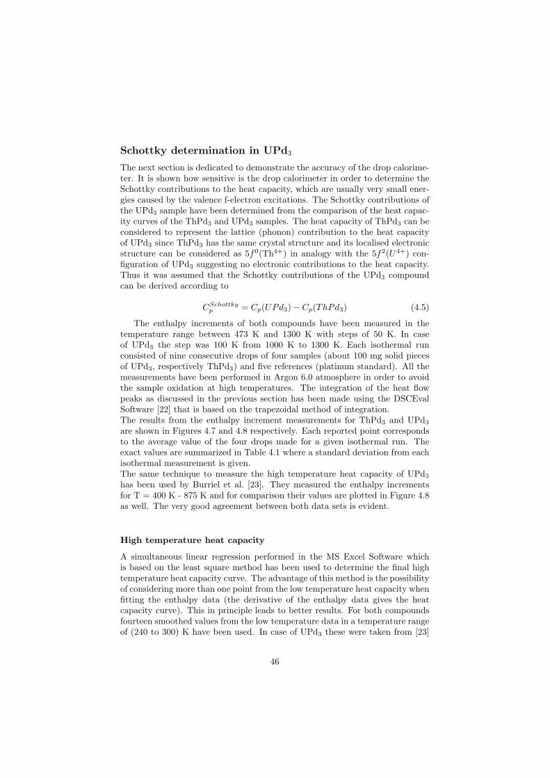
Schottky determination in UPd3

The next section is dedicated to demonstrate the accuracy of the drop calorime-ter. It is shown how sensitive is the drop calorimeter in order to determine theSchottky contributions to the heat capacity, which are usually very small ener-gies caused by the valence f-electron excitations. The Schottky contributions ofthe UPd3 sample have been determined from the comparison of the heat capac-ity curves of the ThPd3 and UPd3 samples. The heat capacity of ThPd3 can beconsidered to represent the lattice (phonon) contribution to the heat capacityof UPd3 since ThPd3 has the same crystal structure and its localised electronicstructure can be considered as 5f0(Th4+) in analogy with the 5f2(U4+) con-figuration of UPd3 suggesting no electronic contributions to the heat capacity.Thus it was assumed that the Schottky contributions of the UPd3 compoundcan be derived according to

CSchottkyp = Cp(UPd3)− Cp(ThPd3) (4.5)

The enthalpy increments of both compounds have been measured in thetemperature range between 473 K and 1300 K with steps of 50 K. In caseof UPd3 the step was 100 K from 1000 K to 1300 K. Each isothermal runconsisted of nine consecutive drops of four samples (about 100 mg solid piecesof UPd3, respectively ThPd3) and five references (platinum standard). All themeasurements have been performed in Argon 6.0 atmosphere in order to avoidthe sample oxidation at high temperatures. The integration of the heat flowpeaks as discussed in the previous section has been made using the DSCEvalSoftware [22] that is based on the trapezoidal method of integration.The results from the enthalpy increment measurements for ThPd3 and UPd3

are shown in Figures 4.7 and 4.8 respectively. Each reported point correspondsto the average value of the four drops made for a given isothermal run. Theexact values are summarized in Table 4.1 where a standard deviation from eachisothermal measurement is given.The same technique to measure the high temperature heat capacity of UPd3

has been used by Burriel et al. [23]. They measured the enthalpy incrementsfor T = 400 K - 875 K and for comparison their values are plotted in Figure 4.8as well. The very good agreement between both data sets is evident.

High temperature heat capacity

A simultaneous linear regression performed in the MS Excel Software whichis based on the least square method has been used to determine the final hightemperature heat capacity curve. The advantage of this method is the possibilityof considering more than one point from the low temperature heat capacity whenfitting the enthalpy data (the derivative of the enthalpy data gives the heatcapacity curve). This in principle leads to better results. For both compoundsfourteen smoothed values from the low temperature data in a temperature rangeof (240 to 300) K have been used. In case of UPd3 these were taken from [23]

46

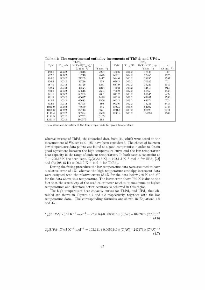
Table 4.1: The experimental enthalpy increments of ThPd3 and UPd3.ThPd3 UPd3

T/K Tref/K H(T)-H(Tref )/ σ T/K Tref/K H(T)-H(Tref )/ σ

(J·mol−1) (J·mol−1) (J·mol−1) (J·mol−1)480.6 303.2 16848 2227 480.6 301.2 18945 147532.7 303.2 19743 2575 532.1 302.2 22455 1575584.6 303.2 27205 1417 584.6 300.2 28695 1557636.3 303.2 32736 578 636.3 303.2 31022 751687.9 303.2 35726 1231 687.9 300.2 39226 1515739.2 303.2 43524 1244 739.2 303.2 44819 913790.2 303.2 50646 2634 790.2 302.2 51850 1848841.1 303.2 53263 2081 841.2 303.2 56945 405891.8 303.2 60687 1428 891.8 302.2 63887 1553942.3 303.2 65683 1556 942.3 303.2 68074 703992.6 303.2 69495 380 992.6 302.2 75231 34141042.9 302.2 74679 155 1092.7 301.8 84297 21441092.8 302.2 82743 3621 1191.9 303.2 97123 29111142.4 302.2 90984 2589 1290.4 303.2 104339 15091191.9 302.2 96762 31051241.3 302.2 101079 482

σ is a standard deviation of the four drops made for given temperature

whereas in case of ThPd3 the smoothed data from [24] which were based on themeasurement of Walker et al. [25] have been considered. The choice of fourteenlow temperature data points was found as a good compromise in order to obtaingood agreement between the high temperature curve and the low temperatureheat capacity in the range of ambient temperature. In both cases a constraint atT = 298.15 K has been kept, Cp(298.15 K) = 102.1 J K−1 mol−1 for UPd3 [23]and Cp(298.15 K) = 99.3 J K−1 mol−1 for ThPd3.

During the fitting procedure the low temperature data were assumed to havea relative error of 1%, whereas the high temperature enthalpy increment datawere assigned with the relative errors of 4% for the data below 750 K and 3%for the data above this temperature. The lower error above 750 K is due to thefact that the sensitivity of the used calorimeter reaches its maximum at highertemperatures and therefore better accuracy is achieved in this region.

The high temperature heat capacity curves for ThPd3 and UPd3 thus ob-tained are shown in Figures 4.7 and 4.8 respectively, together with the lowtemperature data. The corresponding formulas are shown in Equations 4.6and 4.7:

Cp(ThPd3, T )/J K−1 mol−1 = 97.968+0.0086015×(T/K)−109597×(T/K)−2

(4.6)

Cp(UPd3, T )/J K−1 mol−1 = 103.111+0.0059346×(T/K)−247173×(T/K)−2

(4.7)

47

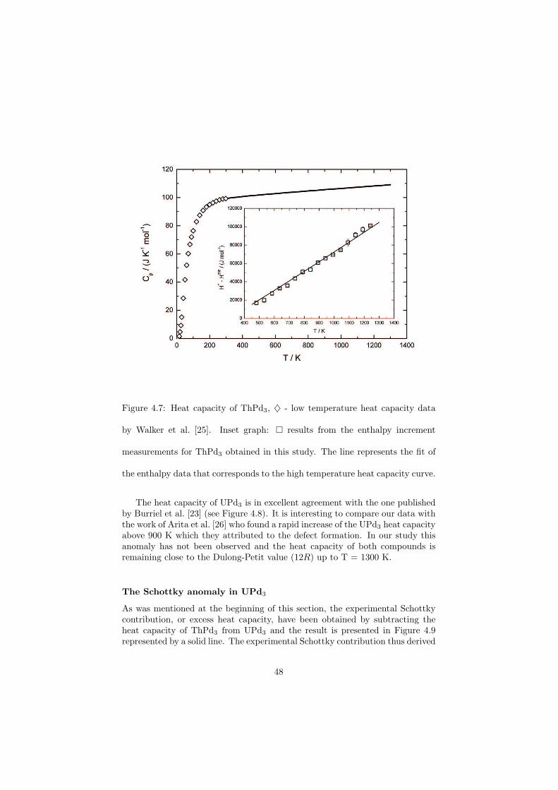
Figure 4.7: Heat capacity of ThPd3, ♦ - low temperature heat capacity data

by Walker et al. [25]. Inset graph: results from the enthalpy increment

measurements for ThPd3 obtained in this study. The line represents the fit of

the enthalpy data that corresponds to the high temperature heat capacity curve.

The heat capacity of UPd3 is in excellent agreement with the one publishedby Burriel et al. [23] (see Figure 4.8). It is interesting to compare our data withthe work of Arita et al. [26] who found a rapid increase of the UPd3 heat capacityabove 900 K which they attributed to the defect formation. In our study thisanomaly has not been observed and the heat capacity of both compounds isremaining close to the Dulong-Petit value (12R) up to T = 1300 K.

The Schottky anomaly in UPd3

As was mentioned at the beginning of this section, the experimental Schottkycontribution, or excess heat capacity, have been obtained by subtracting theheat capacity of ThPd3 from UPd3 and the result is presented in Figure 4.9represented by a solid line. The experimental Schottky contribution thus derived

48

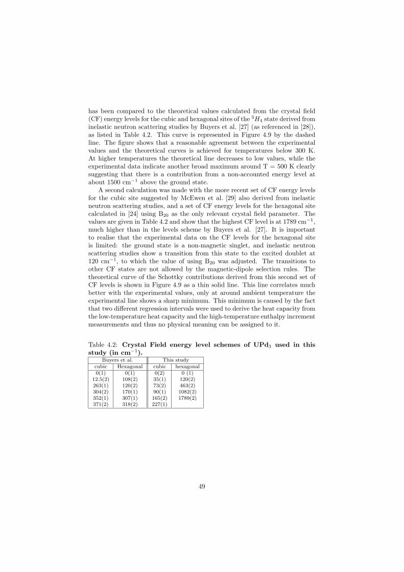
has been compared to the theoretical values calculated from the crystal field(CF) energy levels for the cubic and hexagonal sites of the 3H4 state derived frominelastic neutron scattering studies by Buyers et al. [27] (as referenced in [28]),as listed in Table 4.2. This curve is represented in Figure 4.9 by the dashedline. The figure shows that a reasonable agreement between the experimentalvalues and the theoretical curves is achieved for temperatures below 300 K.At higher temperatures the theoretical line decreases to low values, while theexperimental data indicate another broad maximum around T = 500 K clearlysuggesting that there is a contribution from a non-accounted energy level atabout 1500 cm−1 above the ground state.

A second calculation was made with the more recent set of CF energy levelsfor the cubic site suggested by McEwen et al. [29] also derived from inelasticneutron scattering studies, and a set of CF energy levels for the hexagonal sitecalculated in [24] using B20 as the only relevant crystal field parameter. Thevalues are given in Table 4.2 and show that the highest CF level is at 1789 cm−1,much higher than in the levels scheme by Buyers et al. [27]. It is importantto realise that the experimental data on the CF levels for the hexagonal siteis limited: the ground state is a non-magnetic singlet, and inelastic neutronscattering studies show a transition from this state to the excited doublet at120 cm−1, to which the value of using B20 was adjusted. The transitions toother CF states are not allowed by the magnetic-dipole selection rules. Thetheoretical curve of the Schottky contributions derived from this second set ofCF levels is shown in Figure 4.9 as a thin solid line. This line correlates muchbetter with the experimental values, only at around ambient temperature theexperimental line shows a sharp minimum. This minimum is caused by the factthat two different regression intervals were used to derive the heat capacity fromthe low-temperature heat capacity and the high-temperature enthalpy incrementmeasurements and thus no physical meaning can be assigned to it.

Table 4.2: Crystal Field energy level schemes of UPd3 used in thisstudy (in cm−1).

Buyers et al. This studycubic Hexagonal cubic hexagonal0(1) 0(1) 0(2) 0 (1)

12.5(2) 108(2) 35(1) 120(2)263(1) 120(2) 73(2) 463(2)304(2) 170(1) 90(1) 1082(2)352(1) 307(1) 165(2) 1789(2)371(2) 318(2) 227(1)

49

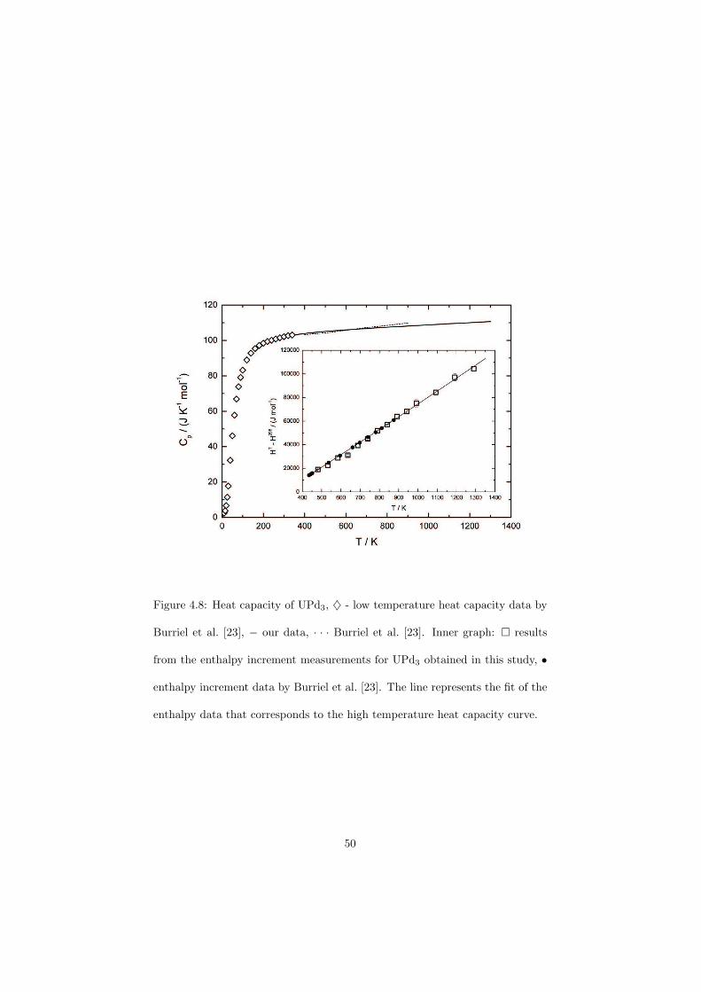
Figure 4.8: Heat capacity of UPd3, ♦ - low temperature heat capacity data by

Burriel et al. [23], − our data, · · · Burriel et al. [23]. Inner graph: results

from the enthalpy increment measurements for UPd3 obtained in this study, •

enthalpy increment data by Burriel et al. [23]. The line represents the fit of the

enthalpy data that corresponds to the high temperature heat capacity curve.

50

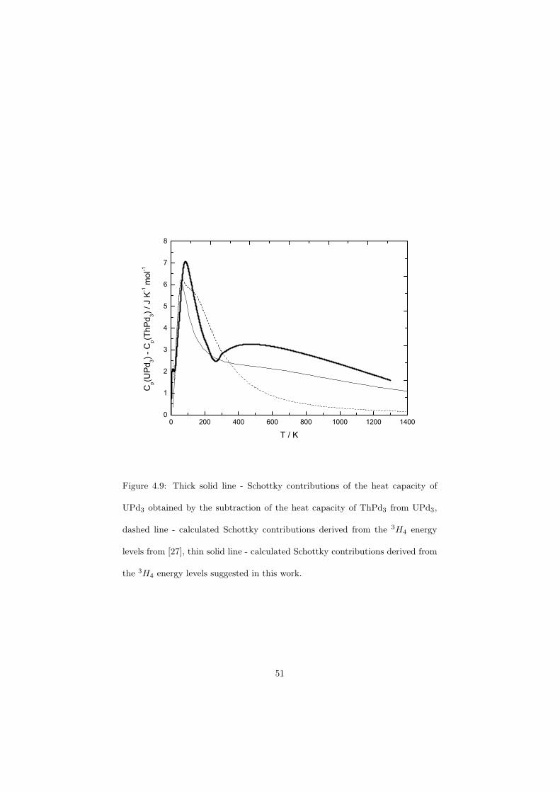
0 200 400 600 800 1000 1200 14000

1

2

3

4

5

6

7

8

Cp(U

Pd

3)

- C

p(T

hP

d3)

/ J K

-1 m

ol-1

T / K

Figure 4.9: Thick solid line - Schottky contributions of the heat capacity of

UPd3 obtained by the subtraction of the heat capacity of ThPd3 from UPd3,

dashed line - calculated Schottky contributions derived from the 3H4 energy

levels from [27], thin solid line - calculated Schottky contributions derived from

the 3H4 energy levels suggested in this work.

51

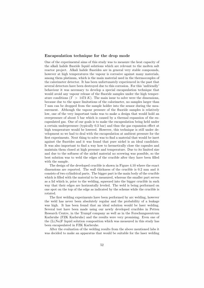
Encapsulation technique for the drop mode

One of the experimental aims of this study was to measure the heat capacity ofthe alkali halide fluoride liquid solutions which are relevant to the molten saltreactor project. Alkali halide fluorides are in general very stable compounds,however at high temperatures the vapour is corrosive against many materials,among them platinum, which is the main material used in the thermocouples ofthe calorimeter detector. It has been unfortunately experienced in the past thatseveral detectors have been destroyed due to this corrosion. For this ’unfriendly’behaviour it was necessary to develop a special encapsulation technique thatwould avoid any vapour release of the fluoride samples under the high temper-ature conditions (T > 1473 K). The main issue to solve were the dimensions,because due to the space limitations of the calorimeter, no samples larger than7 mm can be dropped from the sample holder into the sensor during the mea-surement. Although the vapour pressure of the fluoride samples is relativelylow, one of the very important tasks was to make a design that would hold anoverpressure of about 5 bar which is caused by a thermal expansion of the en-capsulated gas. One of our goals is to make the encapsulation being held undera certain underpressure (typically 0.3 bar) and thus the gas expansion effect athigh temperature would be lowered. However, this technique is still under de-velopment so we had to deal with the encapsulation at ambient pressure for thefirst experiments. Next thing to solve was to find a material that would be inertagainst the fluorides and it was found that pure nickel is an ideal candidate.It was also important to find a way how to hermetically close the capsules andmaintain them closed at high pressure and temperature. Due to its limited sizeand due to the softness of the nickel material no screwing was possible, so thebest solution was to weld the edges of the crucible after they have been filledwith the sample.

The design of the developed crucible is shown in Figure 4.10 where the exactdimensions are reported. The wall thickness of the crucible is 0.2 mm and itconsists of two cylindrical parts. The bigger part is the main body of the cruciblewhich is filled with the material to be measured, whereas the smaller part servesas a lid which is, prior to the welding, squeezed into the bigger crucible in suchway that their edges are horizontally leveled. The weld is being performed onone spot on the top of the edge as indicated by the scheme while the crucible isrotated.

The first welding experiments have been performed by arc welding, howeverthe weld has never been absolutely regular and the probability of a leakagewas high. It has been found that an ideal solution would be laser welding.Several test have been made using our newly developed crucibles in PettenResearch Centre, in the Trumpf company as well as in the ForschungszentrumKarlsruhe (FZK Karlsruhe) and the results were very promising. Even one ofthe (Li,Na)F liquid solution composition which was measured in this study hasbeen encapsulated in FZK Karlsruhe.

After the evaluation of the welding results from the above mentioned labs itwas decided to make an apparatus that would be suitable for the laser welding

52

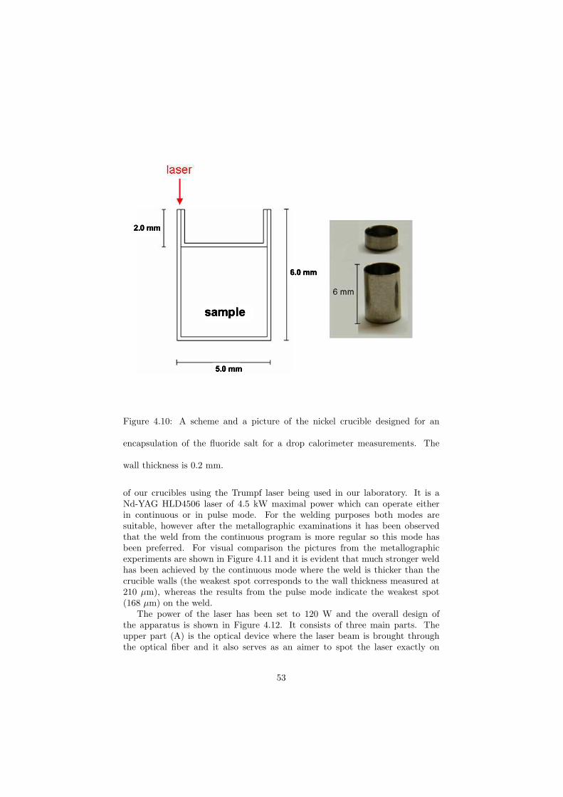
Figure 4.10: A scheme and a picture of the nickel crucible designed for an

encapsulation of the fluoride salt for a drop calorimeter measurements. The

wall thickness is 0.2 mm.

of our crucibles using the Trumpf laser being used in our laboratory. It is aNd-YAG HLD4506 laser of 4.5 kW maximal power which can operate eitherin continuous or in pulse mode. For the welding purposes both modes aresuitable, however after the metallographic examinations it has been observedthat the weld from the continuous program is more regular so this mode hasbeen preferred. For visual comparison the pictures from the metallographicexperiments are shown in Figure 4.11 and it is evident that much stronger weldhas been achieved by the continuous mode where the weld is thicker than thecrucible walls (the weakest spot corresponds to the wall thickness measured at210 µm), whereas the results from the pulse mode indicate the weakest spot(168 µm) on the weld.

The power of the laser has been set to 120 W and the overall design ofthe apparatus is shown in Figure 4.12. It consists of three main parts. Theupper part (A) is the optical device where the laser beam is brought throughthe optical fiber and it also serves as an aimer to spot the laser exactly on

53

the edge of the crucible. The design is made in such way that the opticaldevice is always in a steady position. The middle part (B) is the welding vesselwhere the crucible is fixed during the welding process. As mentioned before,this chamber is connected on the outlet to the vacuum pump and on the inletto the argon supply. It is crucial to have an inert atmosphere during the hightemperature welding so the oxidation of the nickel material is avoided. Moreoverit was necessary to make the crucible holder from copper which is excellent heatconductor and serves as a sink of the heat produced on the edge of the crucibleduring welding. In case of encapsulation of the low melting samples it hasbeen experienced that this heat was large enough to melt the sample inside thecrucible and the overpressure inside the crucible (caused by the gas thermalexpansion) forced the liquid phase to leak. The whole welding vessel is placedon the moveable platform which is used for the laser positioning. The bottompart (C) of the apparatus is the turning device which is connected directly tothe crucible holder and maintains rotating during welding.

The time of one rotation is about 3.5 seconds and one welding sequence hasbeen programmed for 11 seconds. During the first 2 seconds the laser powerincreases reaching the desired 120 W which is kept for other 8 seconds, longenough to make more than two rotations to ensure a smooth weld. During thelast second the laser power linearly decreases to zero value. The graphical formof the designed welding sequence as a function of time is shown in Figure 4.13.

54

Figure 4.11: Metallography of the welded drop crucibles. A: The edge of the

welded crucible using the pulse mode; B: The edge of the welded crucible using

the continuous mode; C: A diametral cut of the crucible welded by the pulse

mode; D: A diametral cut of the crucible welded by the continuos mode

55

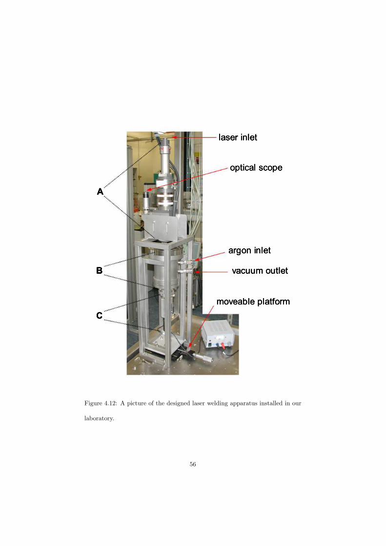
Figure 4.12: A picture of the designed laser welding apparatus installed in our

laboratory.

56

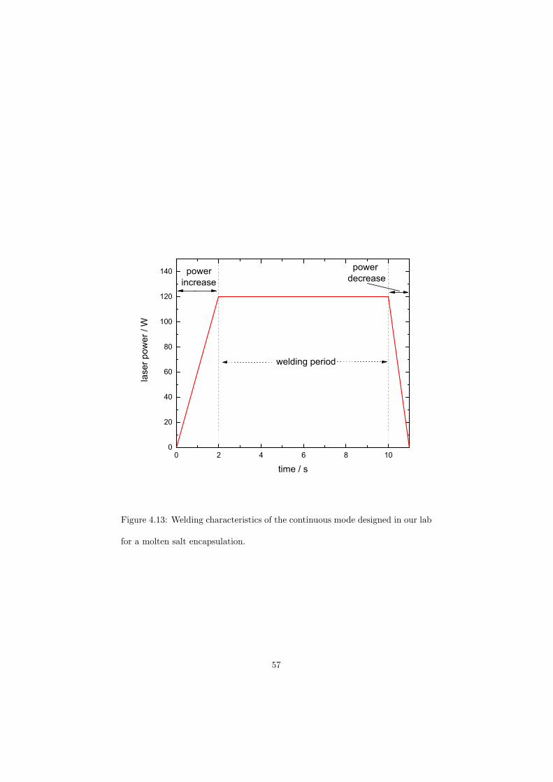
0 2 4 6 8 100

20

40

60

80

100

120

140 power

decrease

lase

r p

ow

er

/ W

time / s

welding period

power

increase

Figure 4.13: Welding characteristics of the continuous mode designed in our lab

for a molten salt encapsulation.

57

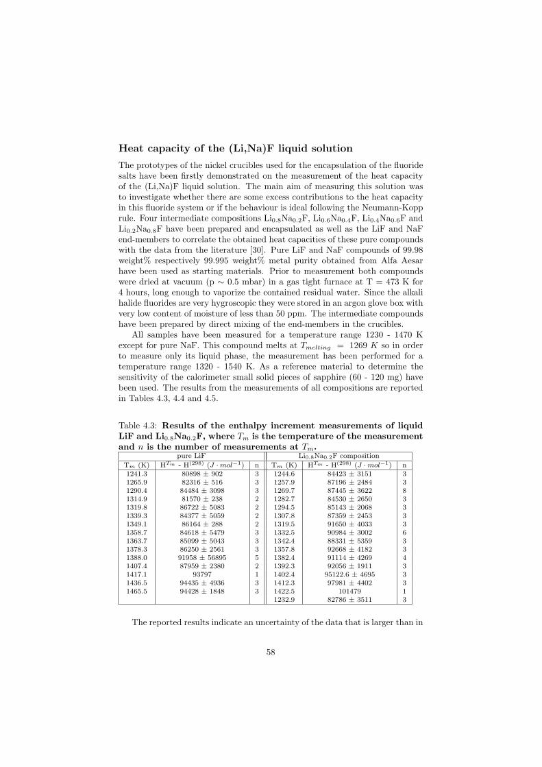
Heat capacity of the (Li,Na)F liquid solution

The prototypes of the nickel crucibles used for the encapsulation of the fluoridesalts have been firstly demonstrated on the measurement of the heat capacityof the (Li,Na)F liquid solution. The main aim of measuring this solution wasto investigate whether there are some excess contributions to the heat capacityin this fluoride system or if the behaviour is ideal following the Neumann-Kopprule. Four intermediate compositions Li0.8Na0.2F, Li0.6Na0.4F, Li0.4Na0.6F andLi0.2Na0.8F have been prepared and encapsulated as well as the LiF and NaFend-members to correlate the obtained heat capacities of these pure compoundswith the data from the literature [30]. Pure LiF and NaF compounds of 99.98weight% respectively 99.995 weight% metal purity obtained from Alfa Aesarhave been used as starting materials. Prior to measurement both compoundswere dried at vacuum (p ∼ 0.5 mbar) in a gas tight furnace at T = 473 K for4 hours, long enough to vaporize the contained residual water. Since the alkalihalide fluorides are very hygroscopic they were stored in an argon glove box withvery low content of moisture of less than 50 ppm. The intermediate compoundshave been prepared by direct mixing of the end-members in the crucibles.

All samples have been measured for a temperature range 1230 - 1470 Kexcept for pure NaF. This compound melts at Tmelting = 1269 K so in orderto measure only its liquid phase, the measurement has been performed for atemperature range 1320 - 1540 K. As a reference material to determine thesensitivity of the calorimeter small solid pieces of sapphire (60 - 120 mg) havebeen used. The results from the measurements of all compositions are reportedin Tables 4.3, 4.4 and 4.5.

Table 4.3: Results of the enthalpy increment measurements of liquidLiF and Li0.8Na0.2F, where Tm is the temperature of the measurementand n is the number of measurements at Tm.

pure LiF Li0.8Na0.2F composition

Tm (K) HTm - H(298) (J ·mol−1) n Tm (K) HTm - H(298) (J ·mol−1) n1241.3 80898 ± 902 3 1244.6 84423 ± 3151 31265.9 82316 ± 516 3 1257.9 87196 ± 2484 31290.4 84484 ± 3098 3 1269.7 87445 ± 3622 81314.9 81570 ± 238 2 1282.7 84530 ± 2650 31319.8 86722 ± 5083 2 1294.5 85143 ± 2068 31339.3 84377 ± 5059 2 1307.8 87359 ± 2453 31349.1 86164 ± 288 2 1319.5 91650 ± 4033 31358.7 84618 ± 5479 3 1332.5 90984 ± 3002 61363.7 85099 ± 5043 3 1342.4 88331 ± 5359 31378.3 86250 ± 2561 3 1357.8 92668 ± 4182 31388.0 91958 ± 56895 5 1382.4 91114 ± 4269 41407.4 87959 ± 2380 2 1392.3 92056 ± 1911 31417.1 93797 1 1402.4 95122.6 ± 4695 31436.5 94435 ± 4936 3 1412.3 97981 ± 4402 31465.5 94428 ± 1848 3 1422.5 101479 1

1232.9 82786 ± 3511 3

The reported results indicate an uncertainty of the data that is larger than in

58

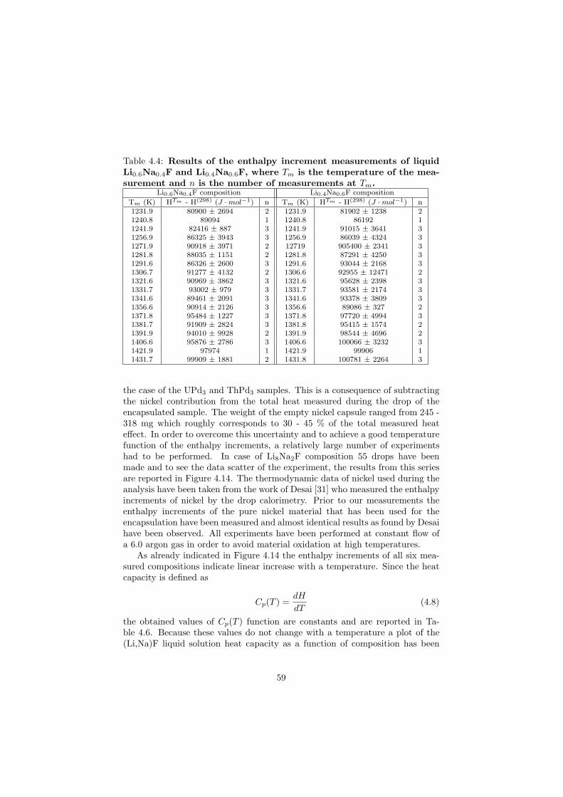
Table 4.4: Results of the enthalpy increment measurements of liquidLi0.6Na0.4F and Li0.4Na0.6F, where Tm is the temperature of the mea-surement and n is the number of measurements at Tm.

Li0.6Na0.4F composition Li0.4Na0.6F composition

Tm (K) HTm - H(298) (J ·mol−1) n Tm (K) HTm - H(298) (J ·mol−1) n1231.9 80900 ± 2694 2 1231.9 81902 ± 1238 21240.8 89094 1 1240.8 86192 11241.9 82416 ± 887 3 1241.9 91015 ± 3641 31256.9 86325 ± 3943 3 1256.9 86039 ± 4324 31271.9 90918 ± 3971 2 12719 905400 ± 2341 31281.8 88035 ± 1151 2 1281.8 87291 ± 4250 31291.6 86326 ± 2600 3 1291.6 93044 ± 2168 31306.7 91277 ± 4132 2 1306.6 92955 ± 12471 21321.6 90969 ± 3862 3 1321.6 95628 ± 2398 31331.7 93002 ± 979 3 1331.7 93581 ± 2174 31341.6 89461 ± 2091 3 1341.6 93378 ± 3809 31356.6 90914 ± 2126 3 1356.6 89086 ± 327 21371.8 95484 ± 1227 3 1371.8 97720 ± 4994 31381.7 91909 ± 2824 3 1381.8 95415 ± 1574 21391.9 94010 ± 9928 2 1391.9 98544 ± 4696 21406.6 95876 ± 2786 3 1406.6 100066 ± 3232 31421.9 97974 1 1421.9 99906 11431.7 99909 ± 1881 2 1431.8 100781 ± 2264 3

the case of the UPd3 and ThPd3 samples. This is a consequence of subtractingthe nickel contribution from the total heat measured during the drop of theencapsulated sample. The weight of the empty nickel capsule ranged from 245 -318 mg which roughly corresponds to 30 - 45 % of the total measured heateffect. In order to overcome this uncertainty and to achieve a good temperaturefunction of the enthalpy increments, a relatively large number of experimentshad to be performed. In case of Li8Na2F composition 55 drops have beenmade and to see the data scatter of the experiment, the results from this seriesare reported in Figure 4.14. The thermodynamic data of nickel used during theanalysis have been taken from the work of Desai [31] who measured the enthalpyincrements of nickel by the drop calorimetry. Prior to our measurements theenthalpy increments of the pure nickel material that has been used for theencapsulation have been measured and almost identical results as found by Desaihave been observed. All experiments have been performed at constant flow ofa 6.0 argon gas in order to avoid material oxidation at high temperatures.

As already indicated in Figure 4.14 the enthalpy increments of all six mea-sured compositions indicate linear increase with a temperature. Since the heatcapacity is defined as

Cp(T ) =dH

dT(4.8)

the obtained values of Cp(T ) function are constants and are reported in Ta-ble 4.6. Because these values do not change with a temperature a plot of the(Li,Na)F liquid solution heat capacity as a function of composition has been

59

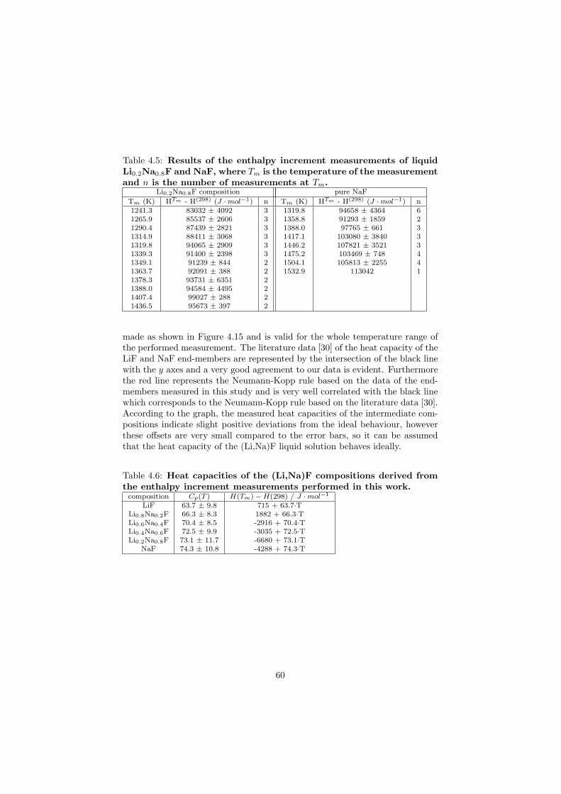
Table 4.5: Results of the enthalpy increment measurements of liquidLi0.2Na0.8F and NaF, where Tm is the temperature of the measurementand n is the number of measurements at Tm.

Li0.2Na0.8F composition pure NaF

Tm (K) HTm - H(298) (J ·mol−1) n Tm (K) HTm - H(298) (J ·mol−1) n1241.3 83032 ± 4092 3 1319.8 94658 ± 4364 61265.9 85537 ± 2606 3 1358.8 91293 ± 1859 21290.4 87439 ± 2821 3 1388.0 97765 ± 661 31314.9 88411 ± 3068 3 1417.1 103080 ± 3840 31319.8 94065 ± 2909 3 1446.2 107821 ± 3521 31339.3 91400 ± 2398 3 1475.2 103469 ± 748 41349.1 91239 ± 844 2 1504.1 105813 ± 2255 41363.7 92091 ± 388 2 1532.9 113042 11378.3 93731 ± 6351 21388.0 94584 ± 4495 21407.4 99027 ± 288 21436.5 95673 ± 397 2

made as shown in Figure 4.15 and is valid for the whole temperature range ofthe performed measurement. The literature data [30] of the heat capacity of theLiF and NaF end-members are represented by the intersection of the black linewith the y axes and a very good agreement to our data is evident. Furthermorethe red line represents the Neumann-Kopp rule based on the data of the end-members measured in this study and is very well correlated with the black linewhich corresponds to the Neumann-Kopp rule based on the literature data [30].According to the graph, the measured heat capacities of the intermediate com-positions indicate slight positive deviations from the ideal behaviour, howeverthese offsets are very small compared to the error bars, so it can be assumedthat the heat capacity of the (Li,Na)F liquid solution behaves ideally.

Table 4.6: Heat capacities of the (Li,Na)F compositions derived fromthe enthalpy increment measurements performed in this work.

composition Cp(T ) H(Tm)−H(298) / J ·mol−1

LiF 63.7 ± 9.8 715 + 63.7·TLi0.8Na0.2F 66.3 ± 8.3 1882 + 66.3·TLi0.6Na0.4F 70.4 ± 8.5 -2916 + 70.4·TLi0.4Na0.6F 72.5 ± 9.9 -3035 + 72.5·TLi0.2Na0.8F 73.1 ± 11.7 -6680 + 73.1·T

NaF 74.3 ± 10.8 -4288 + 74.3·T

60

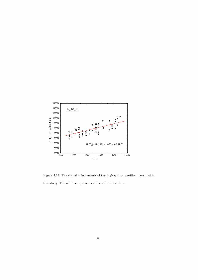
1200 1250 1300 1350 1400 145065000

70000

75000

80000

85000

90000

95000

100000

105000

110000

115000

H (

Tm)

- H

(2

98

) / J/m

ol

T / K

H (Tm) - H (298) = 1882 + 66.29 T

Li0.8

Na0.2

F

Figure 4.14: The enthalpy increments of the Li8Na2F composition measured in

this study. The red line represents a linear fit of the data.

61

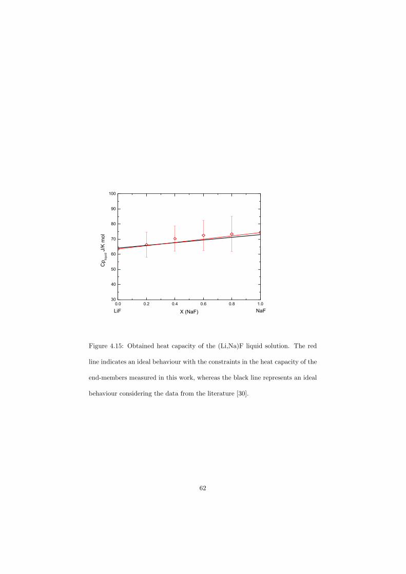
0.0 0.2 0.4 0.6 0.8 1.030

40

50

60

70

80

90

100

Cp

liqu

id J

/K m

ol

X (NaF)LiF NaF

Figure 4.15: Obtained heat capacity of the (Li,Na)F liquid solution. The red

line indicates an ideal behaviour with the constraints in the heat capacity of the

end-members measured in this work, whereas the black line represents an ideal

behaviour considering the data from the literature [30].

62

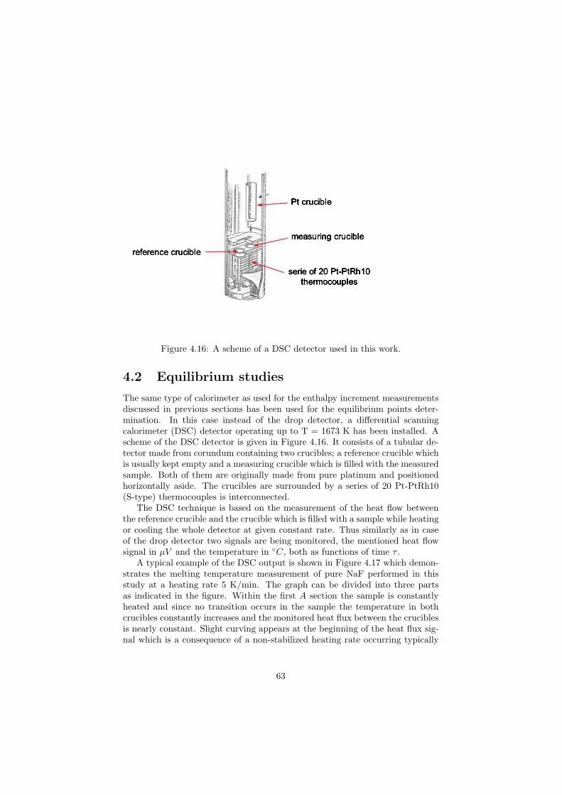
Figure 4.16: A scheme of a DSC detector used in this work.

4.2 Equilibrium studies

The same type of calorimeter as used for the enthalpy increment measurementsdiscussed in previous sections has been used for the equilibrium points deter-mination. In this case instead of the drop detector, a differential scanningcalorimeter (DSC) detector operating up to T = 1673 K has been installed. Ascheme of the DSC detector is given in Figure 4.16. It consists of a tubular de-tector made from corundum containing two crucibles; a reference crucible whichis usually kept empty and a measuring crucible which is filled with the measuredsample. Both of them are originally made from pure platinum and positionedhorizontally aside. The crucibles are surrounded by a series of 20 Pt-PtRh10(S-type) thermocouples is interconnected.

The DSC technique is based on the measurement of the heat flow betweenthe reference crucible and the crucible which is filled with a sample while heatingor cooling the whole detector at given constant rate. Thus similarly as in caseof the drop detector two signals are being monitored, the mentioned heat flowsignal in µV and the temperature in C, both as functions of time τ .

A typical example of the DSC output is shown in Figure 4.17 which demon-strates the melting temperature measurement of pure NaF performed in thisstudy at a heating rate 5 K/min. The graph can be divided into three partsas indicated in the figure. Within the first A section the sample is constantlyheated and since no transition occurs in the sample the temperature in bothcrucibles constantly increases and the monitored heat flux between the cruciblesis nearly constant. Slight curving appears at the beginning of the heat flux sig-nal which is a consequence of a non-stabilized heating rate occurring typically

63

at the beginning of the measured sequence.Once the melting temperature of NaF is reached an extra heat is consumed

in order to melt the whole sample. Since the calorimeter is constantly increasingtemperature the reference crucible follows this trend whereas the temperatureof the measuring crucible is delayed and a thermal gradient between them isachieved. At this stage the heat is being delivered from the hotter, reference,crucible to the colder, sample, one and consequently the heat flow signal changesits slope resulting into a peak as shown in section B in the figure. From thispeak the melting temperature is identified as the intersection of the linear ex-trapolation of the background before the peak and the first inflection tangentas shown on the picture. A similar approach has been already described in theprevious section in Figure 4.3 discussing the drop calorimetry method.

As highlighted in Figure 4.17 the melting temperature of NaF found in ourstudy is Tmelting = 1268.6 K (this temperature is already corrected by thecalibration curve), thus almost the same value as reported Tmelting = 1269 Kfrom the literature [30].

After the transition is complete the heat flow signal is stabilized and is againcharacterized by a smooth line as shown in section C. It is important to notethat the slope of the heat flow signal after the transition does not have to bethe same as prior to the transition. Its actual trend is highly dependent on theheat capacity of the measured material which is usually different for differentphases.

A similar graph as shown in Figure 4.17 is given in Figure 4.18 where the heatflow signal is plotted as a function of temperature (red line) and compared to thecalculated enthalpy temperature function of pure NaF (blue line). According tothis graph the heat flow signal from the DSC measurement can be discussed interms of enthalpy change. Upon heating prior to the transition the enthalpy ofthe sample gradually increases with the temperature and the heat flow signal ischaracterized by a smooth line. At the melting point the enthalpy is changedisothermally by an amount corresponding to Hmelting of NaF. At this pointthe temperature of the sample remains constant until all the material is moltenwhile the heat is being added and a peak on the heat flow signal is observed.The onset temperature of the peak corresponds to the melting point and isvery well correlated to the discontinuity on the enthalpy curve. Since a meltingprocess is a first order transition assigned to one temperature, in ideal case theshape of any peak would be a straight infinite vertical line with the endpointat the same spot as the onset. However due to the thermal conductivity thatdelays the heat transfer in the sensor this is not possible and thus the peak hasfinite shape and posses of some, although very small, width. The total area ofthe peak corresponds to the total enthalpy of melting.

Above the transition point the enthalpy function gradually increases againand the heat flow signal is characterized by a smooth line.

64

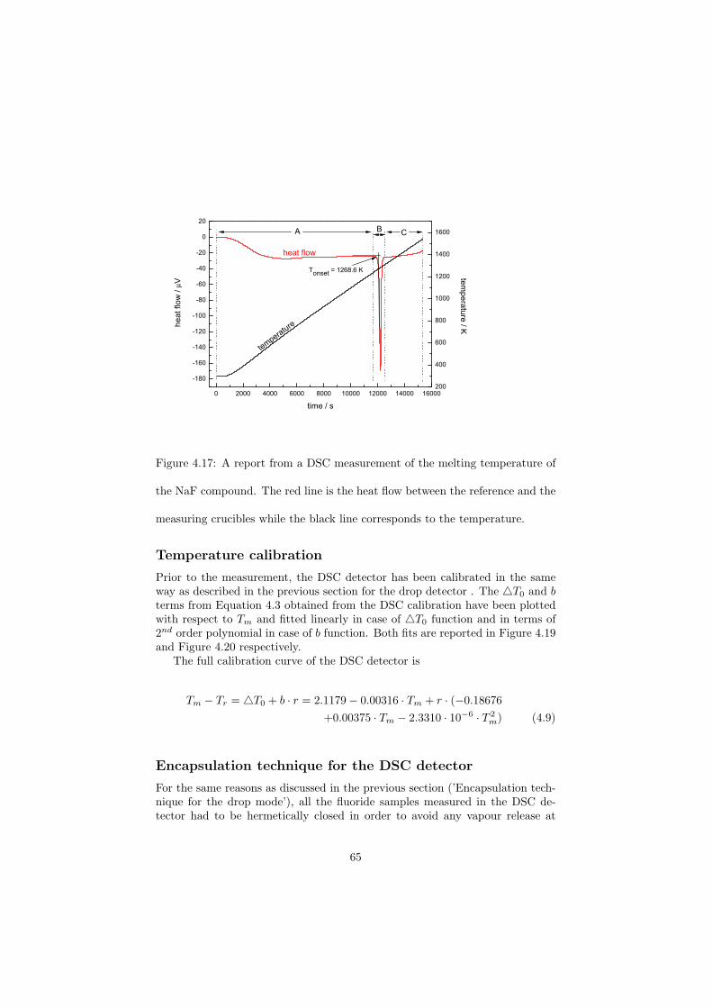
0 2000 4000 6000 8000 10000 12000 14000 16000

-180

-160

-140

-120

-100

-80

-60

-40

-20

0

20

200

400

600

800

1000

1200

1400

1600

he

at flo

w / µ

V

time / s

tem

pe

ratu

re / K

heat flow

tem

peratu

re

Tonset

= 1268.6 K

A B C

Figure 4.17: A report from a DSC measurement of the melting temperature of

the NaF compound. The red line is the heat flow between the reference and the

measuring crucibles while the black line corresponds to the temperature.

Temperature calibration

Prior to the measurement, the DSC detector has been calibrated in the sameway as described in the previous section for the drop detector . The T0 and bterms from Equation 4.3 obtained from the DSC calibration have been plottedwith respect to Tm and fitted linearly in case of T0 function and in terms of2nd order polynomial in case of b function. Both fits are reported in Figure 4.19and Figure 4.20 respectively.

The full calibration curve of the DSC detector is

Tm − Tr = T0 + b · r = 2.1179− 0.00316 · Tm + r · (−0.18676

+0.00375 · Tm − 2.3310 · 10−6 · T 2m) (4.9)

Encapsulation technique for the DSC detector

For the same reasons as discussed in the previous section (’Encapsulation tech-nique for the drop mode’), all the fluoride samples measured in the DSC de-tector had to be hermetically closed in order to avoid any vapour release at

65

400 600 800 1000 1200 1400 1600

-180

-160

-140

-120

-100

-80

-60

-40

-20

0

20

40

60

80

100

-640000

-620000

-600000

-580000

-560000

-540000

-520000

-500000

-480000

-460000

he

at flo

w / µ

V

T / K

H(T

) / J m

ol -1

H(T)

heat flow

peak onset

Figure 4.18: A DSC heat flow signal from the melting temperature measure-

ment of pure NaF as a function of temperature (red line) in comparison to the

calculated enthalpy temperature function of pure NaF (blue line).

high temperatures. It was necessary to make such design that the dimensionsof the crucible would perfectly fit into the sample compartment of the DSCdetector which is required to keep a very good thermal contact. It is also re-quired that the crucible is firm enough to hold the overpressure caused by a gasthermal expansion up to 1673 K (maximal operating temperature of the usedDSC) without deforming because even a slight deformation could damage thedetector since the gap between the crucible and the detector tube is minimal.Furthermore the design had to enable to re-used the crucible after the measure-ment. However this option has been fulfilled only in case of the measurement ofthe NaNO3-KNO3 phase diagram due to the relatively low melting temperatureof the nitrates on one hand side, and on the other the nitrates are very wellsoluble in a water so perfect clean-up of the used crucible could have been per-formed after each measurement. This was not the case of the fluoride sampleswhich melt at higher temperatures, and the opening of the crucibles after thehigh temperature treatment was more difficult due to the steel sintering on thescrews. Nevertheless even if the opening was possible the contamination fromthe sample vapour on the inside walls of the crucible was significant and sincethe fluorides are very insoluble in any solvent that would be non-reactive withstainless steel (best solvent is diluted HF) an absolute clean-up was impossible.

Finally it was necessary to design the crucible from a material that would

66

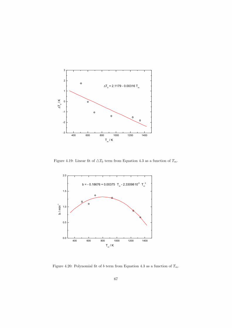
400 600 800 1000 1200 1400-3

-2

-1

0

1

2

3

∆T

0 / K

Tm / K

∆T0 = 2.1179 - 0.00316 T

m

Figure 4.19: Linear fit of T0 term from Equation 4.3 as a function of Tm.

400 600 800 1000 1200 14000.0

0.5

1.0

1.5

2.0

b = - 0.18676 + 0.00375 . Tm - 2.33098.10

-6 . T

m

2

b / m

in-1

Tm / K

Figure 4.20: Polynomial fit of b term from Equation 4.3 as a function of Tm.

67

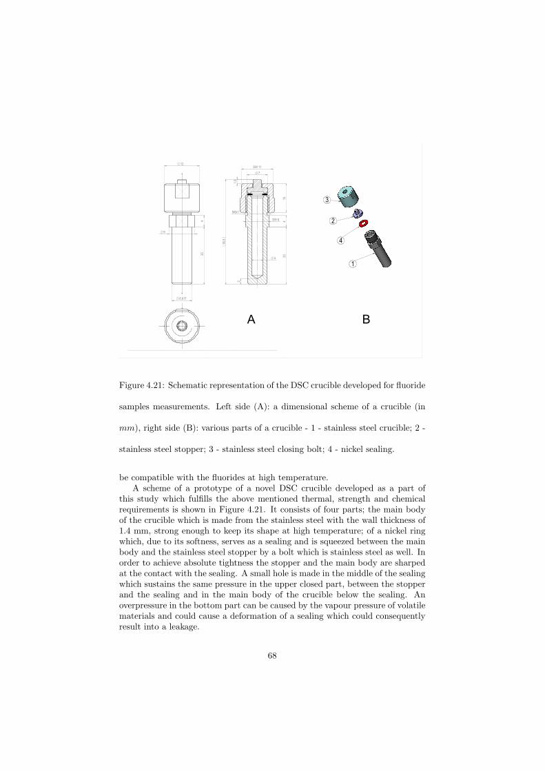
Unterschrift:Datum:

Fertigungszeichnung

GEMEINSAME FORSCHUNGSSTELLE

INSTITUT FÜR TRANSURANE

9

20

6,8 f7

4

12

A

A

SW 8

4

2

36,5

SW 11

204

10

7

1,5

M8x1

A-A

2

1

4

3

POS MENGE BENENNUNG ABMASSE / DIN WERKSTOFF BEMERKUNG ZEICHN.-NR.:1 1 Tiegel Ø9x31 Thermax D-519-13-001.002 1 Blindstopfen Ø7x5 Thermax D-519-13-002.003 1 Mutter Ø12x10 Thermax D-519-13-003.004 1 Dichtung Ø6,8xØ3,5x0,5 Titan

Rz in µmGemittelte Rauhtiefe

DIN ISO 1302 Reihe 2w

R 100

y zx

R 25 R 6.3 R 1 ISO - E

Kommission der Europäischen GemeinschaftenGEMEINSAME FORSCHUNGSSTELLEINSTITUT FÜR TRANSURANE

Karlsruhe

Nennmaß-bereich

von0,5

bis

3

2768-m ±0,1

toleranzenAllgemein-

DIN ISO

über3

bis

6

±0,2 ±0,3 ±0,5 ±0,8 ±1,2 ±2,0±0,1

über über überüber über über6 30 120 400 1000 2000

bis bis bis bis bis bis

30 120 400 1000 2000 4000

NameDatum

gez.

gepr.

03.05.07 Wurzer

ITU - Zeichnungsnummer

Solid Works [A3]

D-519-13-000.00Blatt von

Zust. Änderungs-Nr. Datum Teil DSC-CrucibleMaßstab 4:1

Drop Calorimeter HK

Donnerstag, 3. Mai 2007 16:38:51von Zeichng:DSC-Crucible-Vers.2Modellname: letzte Speicherung vom Model: Donnerstag, 3. Mai 2007 16:40:33

1 1

Template: EUR-A3

A B

Figure 4.21: Schematic representation of the DSC crucible developed for fluoride

samples measurements. Left side (A): a dimensional scheme of a crucible (in

mm), right side (B): various parts of a crucible - 1 - stainless steel crucible; 2 -

stainless steel stopper; 3 - stainless steel closing bolt; 4 - nickel sealing.

be compatible with the fluorides at high temperature.A scheme of a prototype of a novel DSC crucible developed as a part of

this study which fulfills the above mentioned thermal, strength and chemicalrequirements is shown in Figure 4.21. It consists of four parts; the main bodyof the crucible which is made from the stainless steel with the wall thickness of1.4 mm, strong enough to keep its shape at high temperature; of a nickel ringwhich, due to its softness, serves as a sealing and is squeezed between the mainbody and the stainless steel stopper by a bolt which is stainless steel as well. Inorder to achieve absolute tightness the stopper and the main body are sharpedat the contact with the sealing. A small hole is made in the middle of the sealingwhich sustains the same pressure in the upper closed part, between the stopperand the sealing and in the main body of the crucible below the sealing. Anoverpressure in the bottom part can be caused by the vapour pressure of volatilematerials and could cause a deformation of a sealing which could consequentlyresult into a leakage.

68

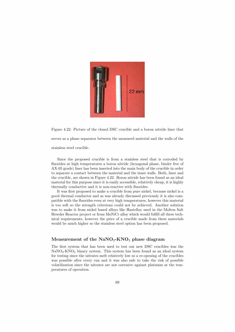
Figure 4.22: Picture of the closed DSC crucible and a boron nitride liner that

serves as a phase separator between the measured material and the walls of the

stainless steel crucible.

Since the proposed crucible is from a stainless steel that is corroded byfluorides at high temperatures a boron nitride (hexagonal phase, binder free ofAX-05 grade) liner has been inserted into the main body of the crucible in orderto separate a contact between the material and the inner walls. Both, liner andthe crucible, are shown in Figure 4.22. Boron nitride has been found as an idealmaterial for this purpose since it is easily accessible, relatively cheap, it is highlythermally conductive and it is non-reactive with fluorides.

It was first proposed to make a crucible from pure nickel, because nickel is agood thermal conductor and as was already discussed previously it is also com-patible with the fluorides even at very high temperatures, however this materialis too soft so the strength criterions could not be achieved. Another solutionwas to make it from nickel based alloys like Hastelloy used in the Molten SaltBreeder Reactor project or from MoNiCr alloy which would fulfill all three tech-nical requirements, however the price of a crucible made from these materialswould be much higher so the stainless steel option has been proposed.

Measurement of the NaNO3-KNO3 phase diagram

The first system that has been used to test our new DSC crucibles was theNaNO3-KNO3 binary system. This system has been found as an ideal systemfor testing since the nitrates melt relatively low so a re-opening of the crucibleswas possible after every run and it was also safe to take the risk of possiblevolatilization since the nitrates are not corrosive against platinum at the tem-peratures of operation.

69

Moreover this system is considered as heat transfer salt for a Generation IVreactors so its melting knowledge is of great importance.

There have been however several studies performed for this system, but inthe literature there are two different versions of this system, one suggesting con-tinuous solid solution [32–41], whereas a recent study [42] indicates an eutecticsystem with limited solubility in the solid state at both NaNO3 and KNO3

end-members. Both versions are shown in Figure 4.23. One of our task was toconfirm which of these published phase diagrams is the correct one.

Pure NaNO3 and KNO3 compounds, both from Alfa Aesar of 99.999 respec-tively 99.994 weight% metal purity have been used as starting materials. Theirmelting temperatures have been measured as well and a very good agreementto the literature data [44] has been found. In case of pure NaNO3 the observedmelting temperature was Tmelting = 579.6 K compared to 579 K from [44]and in case of pure KNO3 the measured melting point was Tmelting = 606.8 Kwhereas a value of 606 K is reported in [44] reports.

The mixtures have been prepared by direct mixing in the crucibles to achievea minimal composition errors. After the crucibles were closed they were insertedinto the calorimeter and measured. For each composition three heating andcooling runs have been made in total. The first heating and cooling cycle hasbeen made to achieve perfect mixing of the sample and the results from this runhave never been taken into account. The other two cycles have been analyzedand the obtained results are reported in Table 4.7. The temperature range ofall experiments was 293 - 673 K, thus the peak temperature was higher thanthe melting temperature of pure KNO3, the higher melting end-member. Theheating rates were 3 and 5 K/min and from both measurement nearly identicalresults have been obtained. Due to the supercooling effect of the nitrate saltsthe results from the cooling sequences have never been taken into account.

All the data from Table 4.7 are also reported in Figure 4.24 and it is ev-ident that due to the measured eutectoid in the solid state rather continuoussolid solubility with a minimum on the liquidus line is confirmed. Hence ac-cording to our measurement the bottom picture from Figure 4.23 is selectedas the correct one. The eutectic temperature found in our work correspondsto X(KNO3) = 0.49. Furthermore it has been proved by this series of mea-surements that the developed crucibles are a very promising solution how toencapsulate the fluoride sample while keeping a DSC signal strong enough toidentify the equilibrium points.

Measurement of the RbF-CsF phase diagram

The RbF-CsF binary system has been investigated by Samuseva and Plyushchev[45]. They used thermal analysis to determine the solidus and liquidus points.Their reported phase diagram however shows a temperature minimum on thesolidus curve without a corresponding minimum on the liquidus curve and thatviolates the phase rule. Therefore the solidus and liquidus temperatures of theRbF-CsF system have been re-evaluated using the DSC detector.

70

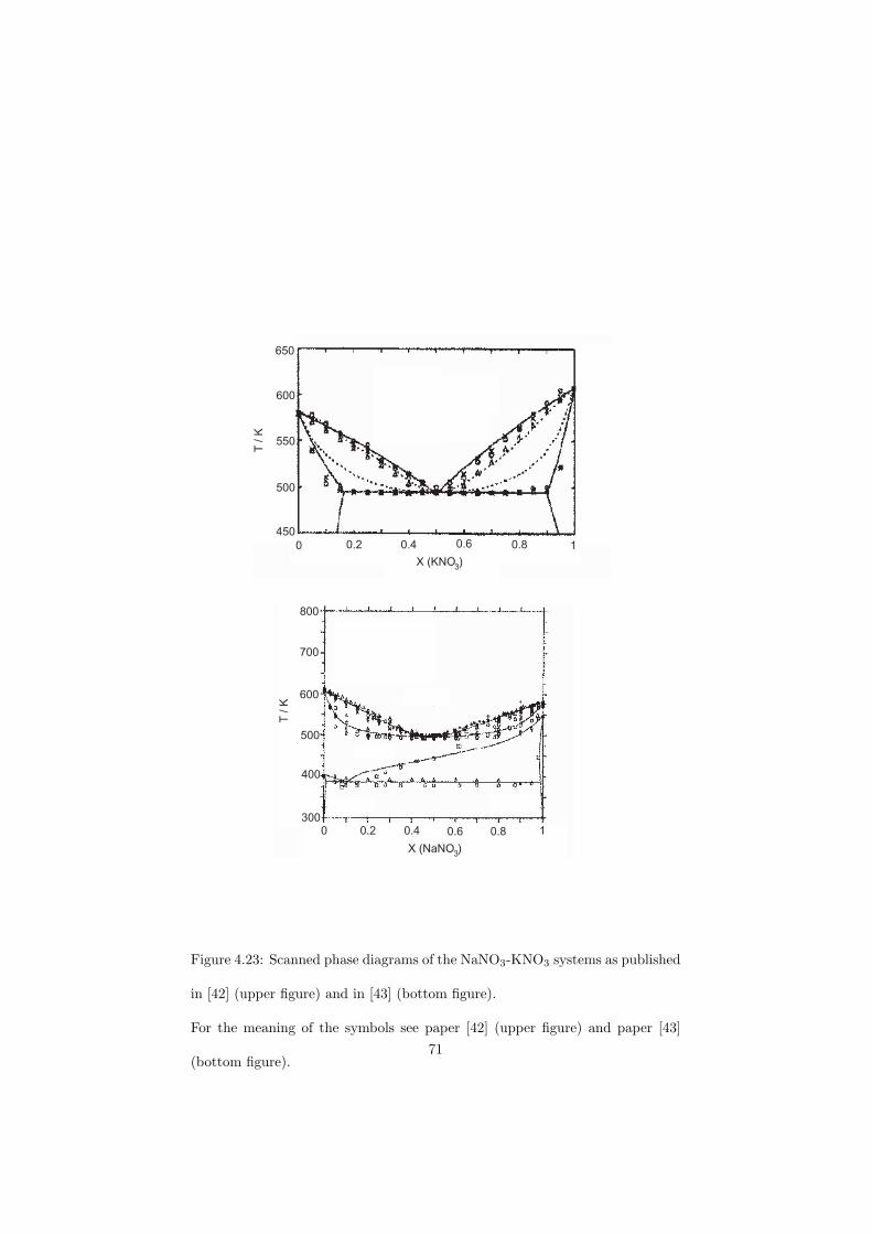
450

500

550

600

650

0 0.2 0.4 0.6 0.8 1

T / K

300

400

500

600

700

800

0 0.2 0.4 0.6 0.8 1

T / K

X (KNO )

X (NaNO )

3

3

Figure 4.23: Scanned phase diagrams of the NaNO3-KNO3 systems as published

in [42] (upper figure) and in [43] (bottom figure).

For the meaning of the symbols see paper [42] (upper figure) and paper [43]

(bottom figure).71

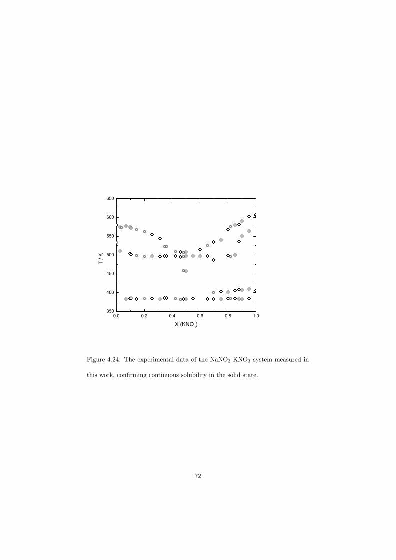
0.0 0.2 0.4 0.6 0.8 1.0350

400

450

500

550

600

650

T / K

X (KNO3)

Figure 4.24: The experimental data of the NaNO3-KNO3 system measured in

this work, confirming continuous solubility in the solid state.

72

The sample preparation has been done by mixing the initial pure RbF (AlfaAesar, 99.975 % metallic purity) and CsF (Alfa Aesar 99.99 % metallic purity)compounds. Since these fluorides are extremely hygroscopic the same procedureas described in case of the measurement of the heat capacity of the (Li,Na)Fliquid solution has been applied. First the pure compounds were dried in argonat T = 180 C for 4 hours and then stored in the dry box. The preparation ofthe intermediate compositions has been performed by direct mixing of RbF andCsF in the DSC crucibles.

Every DSC measurement consisted of three heating and cooling runs. Thefirst run was always used to achieve good mixing between the RbF and CsFcompounds. During this run the salt has been kept for one hour a T=900 C,well above the melting temperature of both components. The data from thisrun have never been considered for analysis. The other two runs were monitoredand both of them consisted of a heating and cooling at a rate of 3K/min andthe peak temperature was 900 C as in case of the pre-run. Since the meltingtemperatures of the pure compounds were well reproduced from the heating andcooling curves, it has been assumed that there is no supercooling effect in thissystem. This observation was also supported by the fact that RbF and CsF arehighly ionic compounds and thus their crystallization is very fast. Therefore itwas possible to analyze the solidus points as the onset points of the DSC peaksfrom the heating curves and the liquidus points as the onset points of the DSCpeaks from the cooling curves. The obtained results are included in Figures 4.28and 4.29 where a comparison to the thermodynamic models (as discussed below)has been made and their exact values are reported in Table 4.8.

Measurement of the CaF2-ThF4 phase diagram

The CaF2-ThF4 system is the last system measured in this study by means ofthe DSC. To our best knowledge it is a system that has not been measured yetby any other authors so novel data are provided in this study. The main interestof measuring this system is the possible use of CaF2 in the matrix of the MSRfuel when designed as a non-moderated breeder reactor as proposed by [8–11].In this concept LiF is used as a carrier salt in which the fertile 232Th and thefissile 235U are dissolved in form of tetrafluorides. According to this conceptthe concentration of ThF4 is about 22-28 mole%, whereas the concentration ofUF4 is relatively low, typically around 1 mole%. Due to the low concentrationsof UF4 and due to the similarities of ThF4 with UF4, the fuel properties canbe estimated based on the LiF-ThF4 binary system which has been assessed inprevious study by van der Meer et al. [46]. The observed eutectic temperaturewas found at T = 836 K that is rather high value for a MSR fuel. Therefore theidea of adding CaF2 into the fuel matrix was established with respect to lowerthe melting temperature.

Since LiF-ThF4 and LiF-CaF2 systems have been already thermodynami-cally described, the unknown CaF2-ThF4 had to be assessed in order to completethe LiF-CaF2-ThF4 ternary. Thus several compositions have been prepared and

73

measured by DSC using our new encapsulation technique. As precursors, an ex-tra dry CaF2 of the 99.999 weight% metal purity obtained from Alfa Aesar wasused, whereas the ThF4 compound was obtained from NRI Rez, Czech Repub-lic. X-ray analysis of this salt has been made prior to the measurement and lessthan 0.5 mole% impurities have been observed. The package of both compoundswas opened and stored in the glove box under a constant flow of argon gas, sothe hydration was avoided. The sample preparation was made by direct mixingof the precursors in the measuring crucibles, similarly as described in case ofthe NaNO3-KNO3 or RbF-CsF experiments.

To avoid the risk of the sample leakage the upper temperature limit of themeasurements was set to 1573 K, thus the melting temperature of pure CaF2

as well as the liquidus data in the CaF2 rich corner could not be observed.However the temperature limit was high enough to determine the liquidus lineof more than 70% of the phase diagram ranging from 0 mole% to 75 mole%of CaF2. The measurement indicate an eutectic at T = 1242 K around 24mole% of CaF2 and a presence of the CaThF6 intermediate compound whichdecomposes peritectically at 1359 K. Further analysis and investigations arenecessary to prove the existence and the range of the (Ca,Th)Fx solid solutionwhich is expected in the CaF2 rich corner. The obtained equilibrium data fromthe measurements as well as the preliminary version of the CaF2-ThF4 phasediagram is shown in Figure 4.25.

74

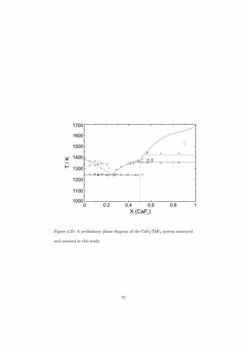
1000

1100

1200

1300

1400

1500

1600

1700

0 10.2 0.4 0.6 0.8

T / K

X (CaF )2

Figure 4.25: A preliminary phase diagram of the CaF2-ThF4 system measured

and assessed in this study.

75

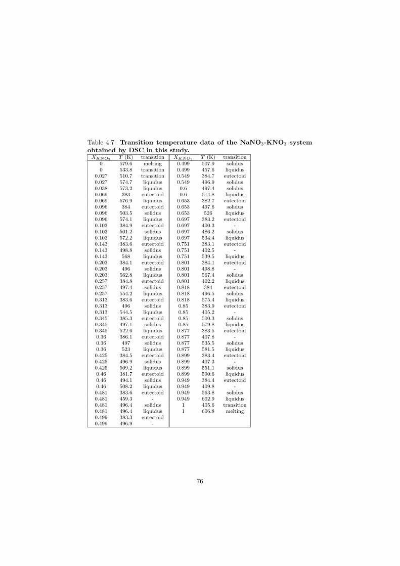
Table 4.7: Transition temperature data of the NaNO3-KNO3 systemobtained by DSC in this study.

XKNO3T (K) transition XKNO3

T (K) transition0 579.6 melting 0.499 507.9 solidus0 533.8 transition 0.499 457.6 liquidus

0.027 510.7 transition 0.549 384.7 eutectoid0.027 574.7 liquidus 0.549 496.9 solidus0.038 573.2 liquidus 0.6 497.4 solidus0.069 383 eutectoid 0.6 514.8 liquidus0.069 576.9 liquidus 0.653 382.7 eutectoid0.096 384 eutectoid 0.653 497.6 solidus0.096 503.5 solidus 0.653 526 liquidus0.096 574.1 liquidus 0.697 383.2 eutectoid0.103 384.9 eutectoid 0.697 400.3 -0.103 501.2 solidus 0.697 486.2 solidus0.103 572.2 liquidus 0.697 534.4 liquidus0.143 383.6 eutectoid 0.751 383.1 eutectoid0.143 498.8 solidus 0.751 402.5 -0.143 568 liquidus 0.751 539.5 liquidus0.203 384.1 eutectoid 0.801 384.1 eutectoid0.203 496 solidus 0.801 498.8 -0.203 562.8 liquidus 0.801 567.4 solidus0.257 384.8 eutectoid 0.801 402.2 liquidus0.257 497.4 solidus 0.818 384 eutectoid0.257 554.2 liquidus 0.818 496.5 solidus0.313 383.6 eutectoid 0.818 575.4 liquidus0.313 496 solidus 0.85 383.9 eutectoid0.313 544.5 liquidus 0.85 405.2 -0.345 385.3 eutectoid 0.85 500.3 solidus0.345 497.1 solidus 0.85 579.8 liquidus0.345 522.6 liquidus 0.877 383.5 eutectoid0.36 386.1 eutectoid 0.877 407.8 -0.36 497 solidus 0.877 535.5 solidus0.36 523 liquidus 0.877 581.5 liquidus0.425 384.5 eutectoid 0.899 383.4 eutectoid0.425 496.9 solidus 0.899 407.3 -0.425 509.2 liquidus 0.899 551.1 solidus0.46 381.7 eutectoid 0.899 590.6 liquidus0.46 494.1 solidus 0.949 384.4 eutectoid0.46 508.2 liquidus 0.949 409.8 -0.481 383.6 eutectoid 0.949 563.8 solidus0.481 459.3 - 0.949 602.9 liquidus0.481 496.4 solidus 1 405.6 transition0.481 496.4 liquidus 1 606.8 melting0.499 383.3 eutectoid0.499 496.9 -

76

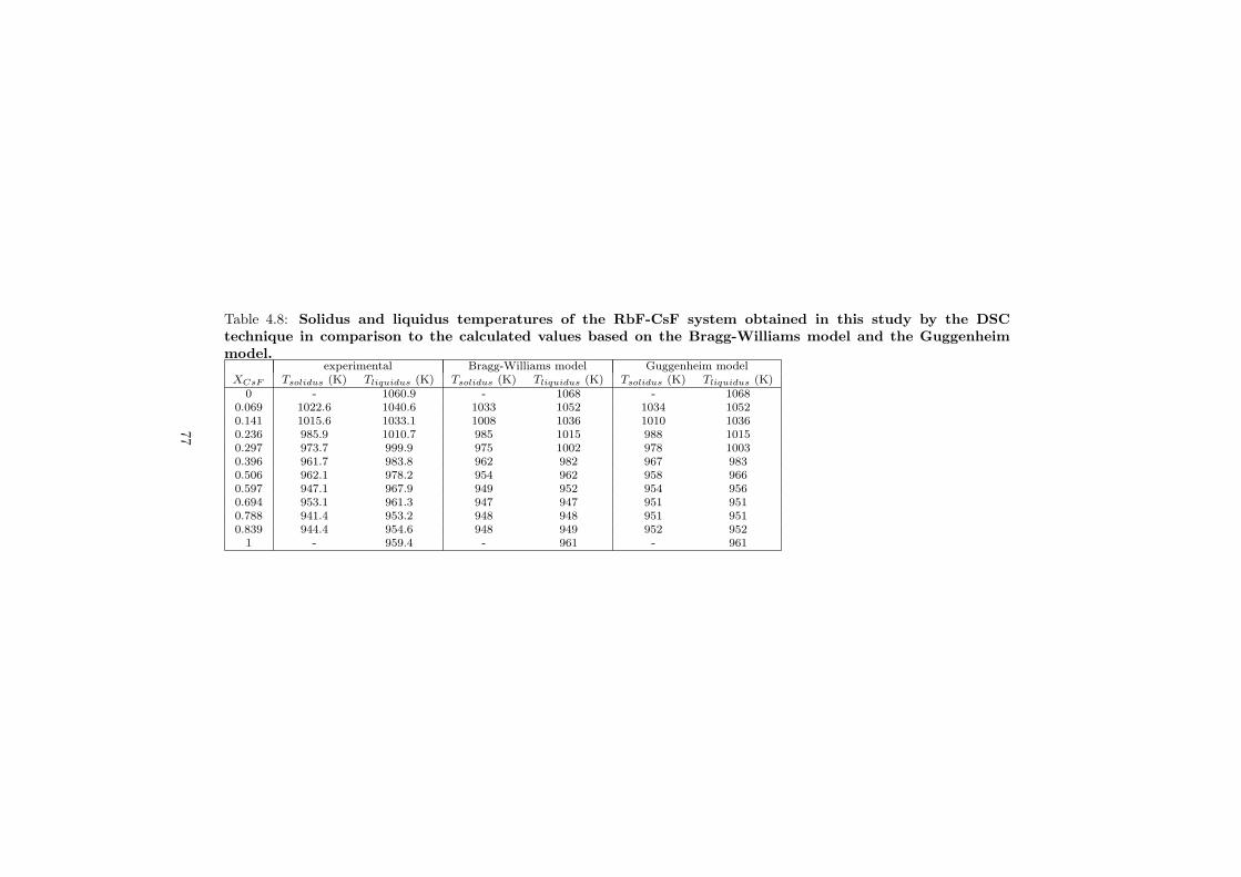
Table 4.8: Solidus and liquidus temperatures of the RbF-CsF system obtained in this study by the DSCtechnique in comparison to the calculated values based on the Bragg-Williams model and the Guggenheimmodel.

experimental Bragg-Williams model Guggenheim modelXCsF Tsolidus (K) Tliquidus (K) Tsolidus (K) Tliquidus (K) Tsolidus (K) Tliquidus (K)

0 - 1060.9 - 1068 - 10680.069 1022.6 1040.6 1033 1052 1034 10520.141 1015.6 1033.1 1008 1036 1010 10360.236 985.9 1010.7 985 1015 988 10150.297 973.7 999.9 975 1002 978 10030.396 961.7 983.8 962 982 967 9830.506 962.1 978.2 954 962 958 9660.597 947.1 967.9 949 952 954 9560.694 953.1 961.3 947 947 951 9510.788 941.4 953.2 948 948 951 9510.839 944.4 954.6 948 949 952 952

1 - 959.4 - 961 - 961

77

4.3 First principle calculations

As it was mentioned at the beginning of this chapter, another method whichis nowadays widely used to obtain the thermodynamic data are the ab initiocalculations. In this study the excess enthalpies of the (Rb,Cs)F continuoussolid solution have been calculated and the results have been used to assess theRbF-CsF phase diagram. A correlation to the measured solidus and liquidusdata from Table 4.8 has been made.

(Rb,Cs)F solid solution

A macroscopic sample made of NRb rubidium atoms, NCs cesium atoms andNRb + NCs fluorine atoms is considered. All the calculations performed in thiswork are done at zero pressure so the pV term is equal to zero and thus theenthalpy is equal to internal energy (H = U) and consequently the free energy isequal to the Gibbs energy (F = G). It must be noted that in order to simulatethe ambient conditions, the p = 1 bar should be assumed. However due to thefact that the condensed phase was matter of our study, the pV term is negligible.

Statistical thermodynamics in the canonical ensemble at absolute tempera-ture T relates the free energy to the partition function Ω which itself is basedon configurational energies through the following formulas

F = −kT lnΩ (4.10)

and

Ω =∑

c

exp

(

−Φ(c)

kBT

)

(4.11)

where c stands for a configuration, i.e. an arrangement of a set of Rb and Csatoms on the cation sublattice, Φ(c) is its hamiltonian energy and kB is theBolzmann constant. In contrast to configuration, a solid solution is a macro-scopic concept encompassing all these microscopic configurations. The weightof a configuration in a given solid solution depends on the external constraintsas described by the thermodynamic variables (p, T, U, S, xRb, xCs, µRb, µCs

etc.).Excess quantities obey similar relationships as shown in two previous Equa-

tions 4.10 and 4.11. In this study it is assumed that configurational energies donot depend on temperature and they are computed for T = 0 K. In other wordsthe vibrational contributions to the excess free energy (FE) are neglected. Thisincludes the so-called zero point energy, i.e. the phonon energy at T = 0 K,since we do not compute any phonon spectrum. Configuration energies are cal-culated ab initio and for a limited number of configurations (in our case 18). Ina second step the relevance of the ”bond” model and the ”Surrounded atom”(SA) model ie discussed in order to extrapolate Φ(c) to just any configurationc involved in Equation 4.11. In the third step either of two approximations,

78

Bragg-Williams and Guggenheim, is used to compute the partition functionΩ as given by Equation 4.11. Although historically the Bragg-Williams andGuggenheim model were presented within the frame of the bond model whereasthe SA model was presented combined with the ”order 1” approximation. Theenergy models are distinguished from the approximations made in the calcula-tion of Ω. Finally the entropy is obtained as S = −

(

∂F∂T

)

Vand internal energy

or enthalpy as H = U = F + TS.It was assumed that disorder does not mix cations with anions since it is

well established that antisite defect in these strongly ionic compounds have avery large positive energy. Accordingly, the configurational energy is attributedto cations only.

ab initio calculations

CASTEP parameters

The calculations have been made using the plane-wave pseudopotential codeCASTEP [47], in close collaboration with CEA using the computational facili-ties in Saclay, France. CASTEP implements density functional theory and hasbeen extensively described elsewhere [47]. The GGA-PBE approximation hasbeen used for the exchange correlation functional. The first Brillouin zone issampled with the Moukhorst-Pack scheme with intervals no larger than 0.040

A−1

on all axes. The Material Studio [48] interface is used for launching thecalculation and analyzing the results. The pseudopotentials are also taken fromthe Material Studio library. For fluorine atom the pseudo atomic calculationhas been performed for F 2s2 2p5 configuration with total energy of -659.0571eV, for rubidium atom the calculation has been performed for Rb 4s2 4p6 5s1

configuration with total energy of -661.5621 eV and for cesium atom the pseudoatomic configuration was Cs 5s2 5p6 6s1 and its total energy was -552.0100 eV.

To identify the best cut-off energy value, several calculations of tetragonalRbCsF2 (P 4

mmm space group) have been performed with the variation of thecut-off energy ranging from 350 eV to 500 eV with the step of 50 eV. It hasbeen found that a satisfactory accuracy has been achieved for the cut-off energyof 400 eV and this value has been selected for all our calculations.

Excess energies calculation

The excess energies of total eighteen different configurations of the (Rb,Cs)Fsolid solution have been calculated using CASTEP. Firstly the energies of thepure RbF and CsF end-members have been determined and these are thenproportionally subtracted from the energies of any (Rb,Cs)F solid solution con-figuration according to Equation 4.12.

Uexcess(RbxCsyFx+y) = U(RbxCsyFx+y)− x · U(RbF )− y · U(CsF ) (4.12)

79

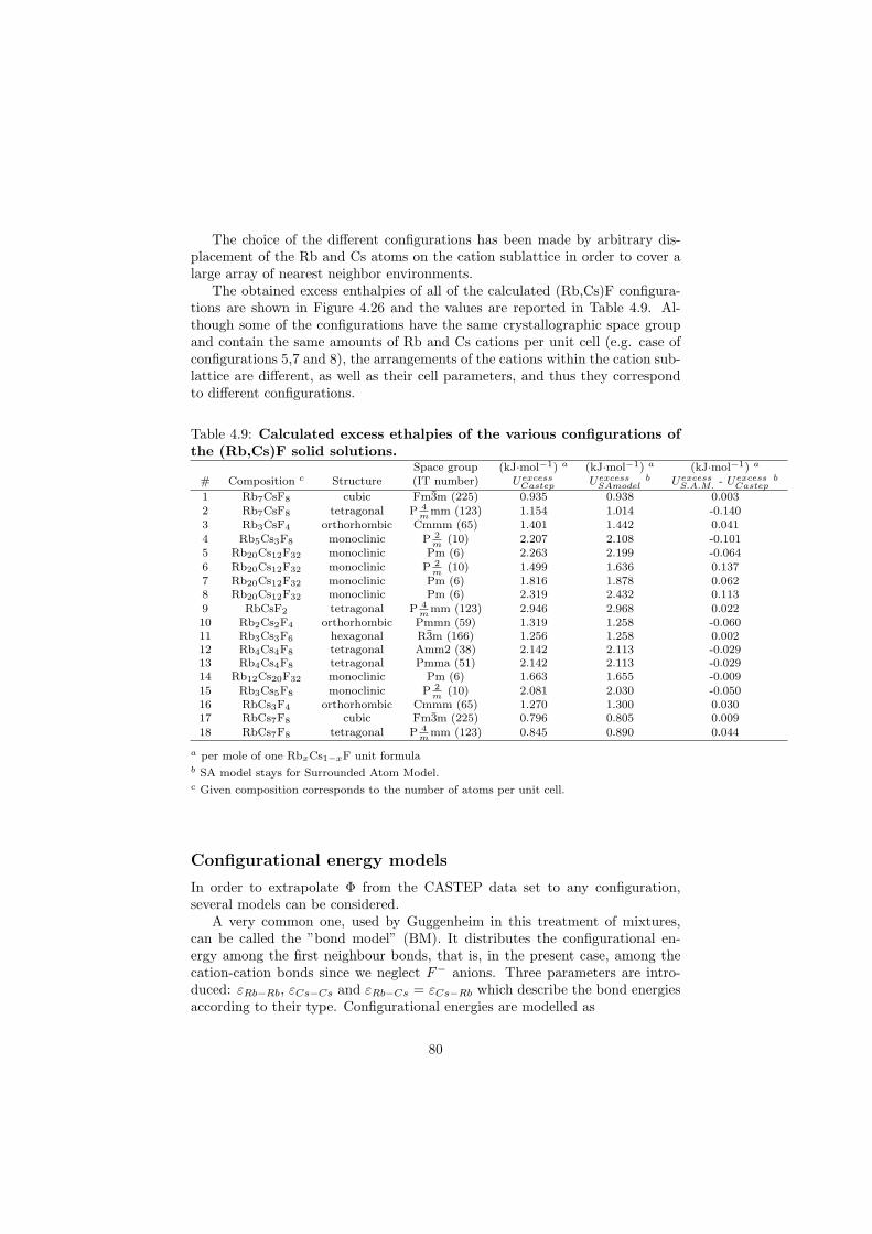
The choice of the different configurations has been made by arbitrary dis-placement of the Rb and Cs atoms on the cation sublattice in order to cover alarge array of nearest neighbor environments.

The obtained excess enthalpies of all of the calculated (Rb,Cs)F configura-tions are shown in Figure 4.26 and the values are reported in Table 4.9. Al-though some of the configurations have the same crystallographic space groupand contain the same amounts of Rb and Cs cations per unit cell (e.g. case ofconfigurations 5,7 and 8), the arrangements of the cations within the cation sub-lattice are different, as well as their cell parameters, and thus they correspondto different configurations.

Table 4.9: Calculated excess ethalpies of the various configurations ofthe (Rb,Cs)F solid solutions.

Space group (kJ·mol−1) a (kJ·mol−1) a (kJ·mol−1) a

# Composition c Structure (IT number) UexcessCastep Uexcess

SAmodelb Uexcess

S.A.M. - UexcessCastep

b

1 Rb7CsF8 cubic Fm3m (225) 0.935 0.938 0.0032 Rb7CsF8 tetragonal P 4

mmm (123) 1.154 1.014 -0.140

3 Rb3CsF4 orthorhombic Cmmm (65) 1.401 1.442 0.0414 Rb5Cs3F8 monoclinic P 2

m(10) 2.207 2.108 -0.101

5 Rb20Cs12F32 monoclinic Pm (6) 2.263 2.199 -0.0646 Rb20Cs12F32 monoclinic P 2

m(10) 1.499 1.636 0.137

7 Rb20Cs12F32 monoclinic Pm (6) 1.816 1.878 0.0628 Rb20Cs12F32 monoclinic Pm (6) 2.319 2.432 0.1139 RbCsF2 tetragonal P 4

mmm (123) 2.946 2.968 0.022

10 Rb2Cs2F4 orthorhombic Pmmn (59) 1.319 1.258 -0.06011 Rb3Cs3F6 hexagonal R3m (166) 1.256 1.258 0.00212 Rb4Cs4F8 tetragonal Amm2 (38) 2.142 2.113 -0.02913 Rb4Cs4F8 tetragonal Pmma (51) 2.142 2.113 -0.02914 Rb12Cs20F32 monoclinic Pm (6) 1.663 1.655 -0.00915 Rb3Cs5F8 monoclinic P 2

m(10) 2.081 2.030 -0.050

16 RbCs3F4 orthorhombic Cmmm (65) 1.270 1.300 0.03017 RbCs7F8 cubic Fm3m (225) 0.796 0.805 0.00918 RbCs7F8 tetragonal P 4

mmm (123) 0.845 0.890 0.044

a per mole of one RbxCs1−xF unit formulab SA model stays for Surrounded Atom Model.c Given composition corresponds to the number of atoms per unit cell.

Configurational energy models

In order to extrapolate Φ from the CASTEP data set to any configuration,several models can be considered.

A very common one, used by Guggenheim in this treatment of mixtures,can be called the ”bond model” (BM). It distributes the configurational en-ergy among the first neighbour bonds, that is, in the present case, among thecation-cation bonds since we neglect F− anions. Three parameters are intro-duced: εRb−Rb, εCs−Cs and εRb−Cs = εCs−Rb which describe the bond energiesaccording to their type. Configurational energies are modelled as

80

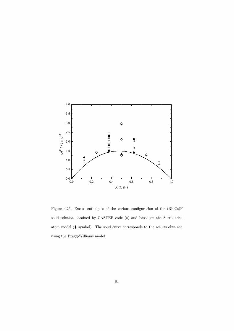
0.0 0.2 0.4 0.6 0.8 1.00.0

0.5

1.0

1.5

2.0

2.5

3.0

3.5

4.0

∆H

E / k

J m

ol-1

X (CsF)

Figure 4.26: Excess enthalpies of the various configuration of the (Rb,Cs)F

solid solution obtained by CASTEP code () and based on the Surrounded

atom model ( symbol). The solid curve corresponds to the results obtained

using the Bragg-Williams model.

81

Φ(a) =z

2(NRbεRbRb + NCsεCsCs) + aω (4.13)

where a is the number of Rb-Cs nearest neighbour pairs in the sample,

ω = εRbCs −εRbRb + εCsCs

2, (4.14)

εij is the energy of an ij bond and z is the lattice dependent coordinationparameter which in case of the (Rb,Cs)F fcc lattice is equal to 12.

The bond model can only be adequately fitted to the CASTEP data set if ωis allowed to be concentration dependent, which is considered not satisfactory,so that we switched to more elaborate treatment provided by the SA model.The SA model has been presented by Mathieu et al. [49, 50] to describe binaryalloys. We apply it here to a pseudo-binary mixture by completely neglectingthe F− anions.

In the following the original derivation by Mathieu et al. is briefly summa-rized, using as much as possible the notations of [49]. The main characteristicof the SA model is the elementary configurational support as a central atom (inour case of cation) in the force field of its z first nearest neighbors on the cationsublattice. This replaces the pair interactions of the ”bond” model describedabove. The excess configurational energy is given by

ΦxcSA(c) = Φc

SA((Mj), (Pi)) = ΦcSA((M1, ...,M12), (P1, ..., P12))

=12∑

j=1

Mj Uj +12∑

i=1

Pi Vi (4.15)

where Mj is the number of Rb atoms having exactly j Cs first neighboursand Pi is the number of Cs atoms having exactly i Rb first neighbours, Uj =

NA(EjRb−E0

Rb) and Vi = NA(EjCs−E0

Cs), where NA is the Avogadro’s number,

EjRb is the corresponding energy contribution of a Rb atom and Ei

Cs of a Csatom.

Fitting Equation 4.15 to CASTEP data requires optimization of 2z param-eters (12 U1...U12 parameters and 12 V1...V12 parameters). This is impossiblebased on the knowledge of ’only’ 18 configurations calculated in this work. Nev-ertheless, in the same way as in the original work by Mathieu et al. [50], it wasobserved that a three-parameter law of variation of Uj and Vi is sufficient in or-der to obtain good agreement between the SA model and the CASTEP results.The parabolic laws used in this study are

Uj = α1j + α2j2 (4.16)

Vi = β1i + β2i2 (4.17)

where α1 = 0, α2, β1 and β2 are the three parameters optimized to:

82

α2 = +76.4 J/mol(cation) (4.18)

β1 = −550.9 J/mol(cation) (4.19)

β2 = +85.2 J/mol(cation) (4.20)

Excess energies obtained from the SA model are plotted in Figure 4.26 nextto CASTEP values and a very good data reproduction is evident. These resultsare also reported in Table 4.9, as well as the difference between the initialCASTEP results and the SA model data giving the maximum absolute error of0.140 J/mol.

According to Mathieu et al. [50] if the Uj and Vi laws from Equation 4.16and 4.17 follow linear laws (α2 = β2 = 0) the SA model is completely equivalentto the bond model with ω = (α1 = β1)/NA and it describes what is normallycalled a ”regular solution”. If a quadratic law is obeyed the solution is asym-metric. The latter case was what we found here for the (Rb,Cs)F solid solutionand is explained by the fact that the substitution of the Cs atom into the RbFcrystal is energetically different than the opposite case of substituting the Rbatom into a crystal of CsF.

Calculation of the partition function

At this point all the terms of the sum in Equation 4.11 are known, at leastformally. To calculate the sum two basic models have been applied, the zero or-der approximation Bragg-Williams model [51] and the first order approximationGuggenheim model [52], also known as quasi-chemical model.

The configurations can be sorted using an auxiliary parameter, say A , suchthat all configurations associated with A = a have the same energy E(a). Thenumber of configurations having A = a is denoted with the degeneracy g(a). Inthe bond model, A is the number of Rb-Cs nearest neighbours pairs, while inthe SA model A is an array of 26 numbers (M0, M1, ...,M12, P0, P1, ..., P12).

What matters here is that any single configuration c can be given a specificvalue a = A(c), be it in the original Guggenheim or in the SA model.

After having grouped all the configurations which have the same value ofA, and therefore the same energy denoted from now on Φ(a), Equation 4.11becomes

Ω =∑

a=all A

g(a)exp

(

−Φ(a)

kBT

)

(4.21)

and the total number of configurations is

N !

NRb!NCs!=

∑

a=all A

g(a) (4.22)

83

Given that g(a) is always positive, there exists a value ¯a such that Equa-tion 4.21 and 4.22 combine into

Ω =N !

NRb!NCs!exp

(

−Φ(¯a)

kBT

)

(4.23)

where ¯a is in general a function of T , NRb and NCs.

Bragg-Williams model

The Bragg-Williams model assumes that ¯a is equal to the value correspondingto a completely disordered solution, denoted a∗. That is, the average number ofCs, resp. Rb nearest neighbours to a given ion is equal to zxCs, (resp. zxRb).

Denoting mj =Mj

Cjz

and pi = Pi

Ciz

where Cjz and Ci

z are the usual combinatorial

symbols

Cjz =

z!

j! (z − j)!(4.24)

Ciz =

z!

i! (z − i)!(4.25)

the excess enthalpy of the RbF-CsF system is given by

ΦxsSA(c) =

12∑

j=0

M∗

j Uj + P ∗i Vi (4.26)

where M∗

j = m∗

j Cjz and P ∗i = p∗i Ci

z,

m∗

j = (1− xRbF )j (xRbF )z−j+1 (4.27)

p∗i = (1− xRbF )z−i+1 (xRbF )i. (4.28)

Obtained enthalpy function is shown in Figure 4.26 together with the cal-culated configurational energies. The peak of the curve corresponds to Hxs =1.502 kJ/mol and xCsF = 0.48, thus a slight asymmetry towards the RbF sideis found. The main characteristics of the Bragg-Williams model are the tem-perature independence and as mentioned previously the solution correspondingto the fit is the one with maximum disorder. Thus this state would be the mostprobable at the infinite temperature.

In this work, in the Bragg-Williams model, the energy of mixing does notdepend on temperature. However this model would be compatible with a lineardependence of ¯Φ ( ¯Φ stands for an average energy of the solid solution) on tem-

perature as can be seen by noting that U = F − T δFδT = ¯Φ − δ ¯Φ

δT and that U istemperature independent. In this paper we neglect the vibrational contributionsand therefore the Uj and Vi terms do not depend on temperature.

84

The quasi-chemical ”Guggenheim” model

If two configurations have a large energy difference, the one with the lowest en-ergy has a significantly larger probability of occurrence and this fact is not takeninto account by the Bragg-Williams model. Therefore the Guggenheim modelhas been applied in order to see the excess energy evaluation with temperature.The formalism of calculating the excess Gibbs function using the data from theSA model has been described by Mathieu et al. [50] as well as in our previousstudy [53] and for details the readers are referred to that study.

The obtained excess Gibbs functions are reported in Figure 4.27 and a com-parison to the excess enthalpy curve based on the Bragg-Williams model is made.It is evident that the Bragg-Williams results posses of higher values which isin agreement to what was said previously that this model corresponds to thethermodynamic state with maximal disorder where all configuration have equalprobabilities of occurrence and thus is characteristic for infinite temperature.

Thermodynamic assessment of the RbF-CsF phase diagram

As described above, two models, Bragg-Williams and Guggenheim model, havebeen used to interpret the ab initio data relative to the solid solution.

In order to simplify and to keep a compatibility with our developed database[54], the results from these models have not been directly used during the assess-ment of the RbF-CsF phase diagram. For the excess Gibbs energy description ofthe (Rb,Cs)F solid solution the classical polynomial formalism generally definedas

Gexcess =n

∑

i,j=1

xi1 · x

j2 · Lij (4.29)

has been used, where Lij are the parameters to be optimized and are writtenin a polynomial form. These coefficients have been obtained by the least squarefit of the results from the Bragg-Williams and Guggenheim models and a verygood agreement has been achieved in both cases. Their respective values aregiven below

GEB−W = XRbF · (1− xRbF ) · 5411 + x2

RbF · (1−XRbF ) · 1168 J mol−1 (4.30)

GEGug. = XRbF ·(1−xRbF )·

(

5423−544000

T (K)

)

+x2RbF ·(1−xRbF )·1500 J mol−1

(4.31)Based on the equations above the RbF-CsF phase diagrams have been cal-

culated and a comparison between both versions has been made as shown inFigure 4.28, where a phase diagram based on the Bragg-Williams model ap-proximation is given, and in Figure 4.29 which is based on the data from

85

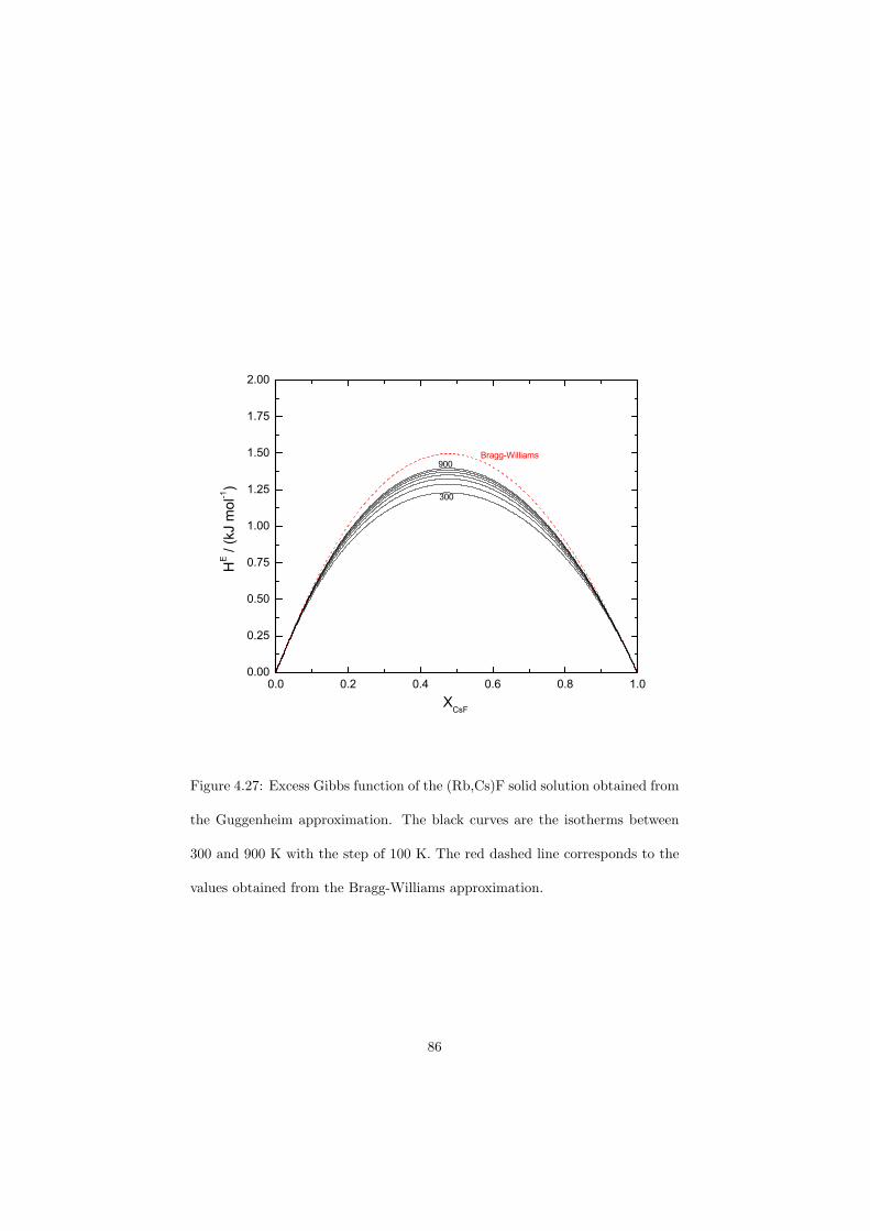
0.0 0.2 0.4 0.6 0.8 1.00.00

0.25

0.50

0.75

1.00

1.25

1.50

1.75

2.00

HE / (

kJ m

ol-1

)

300

900Bragg-Williams

XCsF

Figure 4.27: Excess Gibbs function of the (Rb,Cs)F solid solution obtained from

the Guggenheim approximation. The black curves are the isotherms between

300 and 900 K with the step of 100 K. The red dashed line corresponds to the

values obtained from the Bragg-Williams approximation.

86

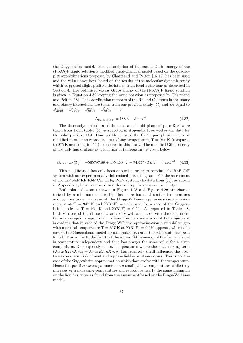
the Guggenheim model. For a description of the excess Gibbs energy of the(Rb,Cs)F liquid solution a modified quasi-chemical model based on the quadru-plet approximations proposed by Chartrand and Pelton [16, 17] has been usedand the values have been based on the results of the molecular dynamic studywhich suggested slight positive deviations from ideal behaviour as described inSection 4. The optimized excess Gibbs energy of the (Rb,Cs)F liquid solutionis given in Equation 4.32 keeping the same notation as proposed by Chartrandand Pelton [18]. The coordination numbers of the Rb and Cs atoms in the unaryand binary interactions are taken from our previous study [55] and are equal toZRb

RbRb = ZCsCsCs = ZRb

RbCs = ZCsRbCs = 6

∆gRbCs/FF = 188.3 J mol−1 (4.32)

The thermodynamic data of the solid and liquid phase of pure RbF weretaken from Janaf tables [56] as reported in Appendix 1, as well as the data forthe solid phase of CsF. However the data of the CsF liquid phase had to bemodified in order to reproduce its melting temperature, T = 961 K (comparedto 975 K according to [56]), measured in this study. The modified Gibbs energyof the CsF liquid phase as a function of temperature is given below

GCsFmod.(T ) = −565797.86 + 405.400 · T − 74.057 · T lnT J mol−1 (4.33)

This modification has only been applied in order to correlate the RbF-CsFsystem with our experimentally determined phase diagram. For the assessmentof the LiF-NaF-KF-RbF-CsF-LaF3-PuF3 system, the data from [56], as shownin Appendix 1, have been used in order to keep the data compatibility.

Both phase diagrams shown in Figure 4.28 and Figure 4.29 are charac-terized by a minimum on the liquidus curve found at similar temperaturesand compositions. In case of the Bragg-Williams approximation the mini-mum is at T = 947 K and X(RbF) = 0.265 and for a case of the Guggen-heim model at T = 951 K and X(RbF) = 0.25. As reported in Table 4.8,both versions of the phase diagrams very well correlates with the experimen-tal solidus-liquidus equilibria, however from a comparison of both figures itis evident that in case of the Bragg-Williams approximation a miscibility gapwith a critical temperature T = 367 K at X(RbF) = 0.576 appears, whereas incase of the Guggenheim model no immiscible region in the solid state has beenfound. This is due to the fact that the excess Gibbs energy of the former modelis temperature independent and thus has always the same value for a givencomposition. Consequently at low temperatures where the ideal mixing term(XRbF RTlnXRbF + XCsF RTlnXCsF ) has relatively small influence, the posi-tive excess term is dominant and a phase field separation occurs. This is not thecase of the Guggenheim approximation which does evolve with the temperature.Hence the positive excess parameters are small at low temperatures while theyincrease with increasing temperature and reproduce nearly the same minimumon the liquidus curve as found from the assessment based on the Bragg-Williamsmodel.

87

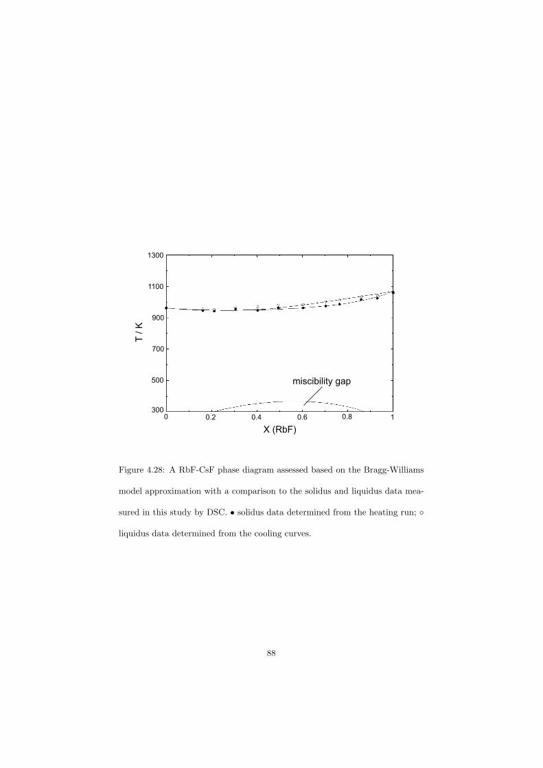
300

500

700

900

1100

1300

0 0.2 0.4 0.6 0.8 1

T / K

X (RbF)

miscibility gap

Figure 4.28: A RbF-CsF phase diagram assessed based on the Bragg-Williams

model approximation with a comparison to the solidus and liquidus data mea-

sured in this study by DSC. • solidus data determined from the heating run;

liquidus data determined from the cooling curves.

88

300

500

700

900

1100

1300

0 0.2 0.4 0.6 0.8 1

X (RbF)

T / K

0 0.40.2 0.6 0.8 1900

950

1000

1050

1100

Figure 4.29: A RbF-CsF phase diagram assessed based on the Guggenheim

model approximation with a comparison to the solidus and liquidus data mea-

sured in this study by DSC. • solidus data determined from the heating run;

liquidus data determined from the cooling curves.

89

Due to the lack of experimental data at low temperature region it is verydifficult to justify which phase diagram is closer to reality, however since theRb+ and Cs+ cations are highly ionic and their sizes are very similar it is notexpected that a miscibility gap would appear in the solid state. Thus the phasediagram shown in Figure 4.29 optimized based on the data of the Guggenheimapproximation is preferred.

90

Chapter 5

Binary systems

In this chapter all the binary phase diagrams that have been assessed as partof this thesis will be discussed. As mentioned previously, the liquid solutionsof most of the systems have been optimized using the modified quasi chemicalmodel proposed by Pelton et al. [16, 17], only the excess Gibbs energies of theliquid solutions of the LiF-ZrF4, UF4-ZrF4, BeF2-ZrF4, BeF2-UF4 and LiF-UF4 systems were optimized using the classical polynomial model. All phasediagrams have been modelled using the FactSage software [14].

This chapter is divided into two sections. In the first one the fluoride systemsare discussed, whereas the other one describes the assessments of the chloridesystems. Most of the systems presented have been optimized based on theknown experimental data, except the BeF2-PuF3 and LaF3-PuF3 binaries forwhich no experimental data are known. Due to the similar nature of the end-members these systems were extrapolated assuming ideal behaviour of theirsolutions. This was however not the case of the KF-PuF3, RbF-PuF3 and CsF-PuF3 systems where no experimental data are available, either. In order toapproximate these three phase diagram the same excess Gibbs parameters asfound in the assessed proxy systems containing LaF3 were used.

91

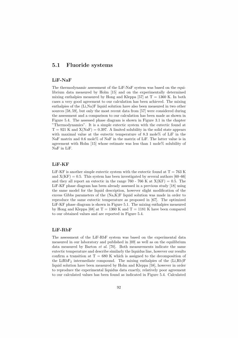
5.1 Fluoride systems

LiF-NaF

The thermodynamic assessment of the LiF-NaF system was based on the equi-librium data measured by Holm [15] and on the experimentally determinedmixing enthalpies measured by Hong and Kleppa [57] at T = 1360 K. In bothcases a very good agreement to our calculation has been achieved. The mixingenthalpies of the (Li,Na)F liquid solution have also been measured in two othersources [58, 59], but only the most recent data from [57] were considered duringthe assessment and a comparison to our calculation has been made as shown inFigure 5.4. The assessed phase diagram is shown in Figure 3.1 in the chapter”Thermodynamics”. It is a simple eutectic system with the eutectic found atT = 921 K and X(NaF) = 0.397. A limited solubility in the solid state appearswith maximal value at the eutectic temperature of 8.3 mole% of LiF in theNaF matrix and 0.6 mole% of NaF in the matrix of LiF. The latter value is inagreement with Holm [15] whose estimate was less than 1 mole% solubility ofNaF in LiF.

LiF-KF

LiF-KF is another simple eutectic system with the eutectic found at T = 763 Kand X(KF) = 0.5. This system has been investigated by several authors [60–66]and they all report an eutectic in the range 760 - 766 K at X(KF) = 0.5. TheLiF-KF phase diagram has been already assessed in a previous study [18] usingthe same model for the liquid description, however slight modification of theexcess Gibbs parameters of the (Na,K)F liquid solution was made in order toreproduce the same eutectic temperature as proposed in [67]. The optimizedLiF-KF phase diagram is shown in Figure 5.1. The mixing enthalpies measuredby Hong and Kleppa [68] at T = 1360 K and T = 1181 K have been comparedto our obtained values and are reported in Figure 5.4.

LiF-RbF

The assessment of the LiF-RbF system was based on the experimental datameasured in our laboratory and published in [69] as well as on the equilibriumdata measured by Barton et al. [70]. Both measurements indicate the sameeutectic temperature and describe similarly the liquidus line, however our resultsconfirm a transition at T = 680 K which is assigned to the decomposition ofthe LiRbF2 intermediate compound. The mixing enthalpies of the (Li,Rb)Fliquid solution have been measured by Holm and Kleppa [58], however in orderto reproduce the experimental liquidus data exactly, relatively poor agreementto our calculated values has been found as indicated in Figure 5.4. Calculated

92

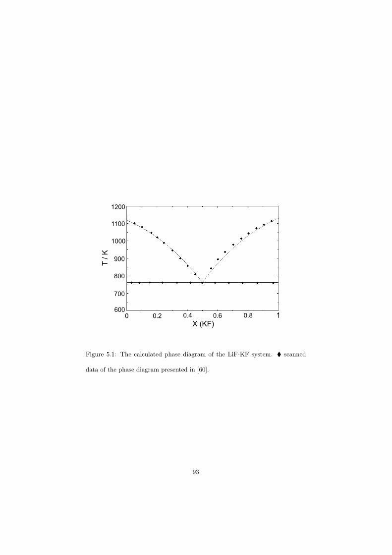
600

700

800

1200

1100

1000

900

0 0.2 0.80.6 10.4

T / K

X (KF)

Figure 5.1: The calculated phase diagram of the LiF-KF system. scanned

data of the phase diagram presented in [60].

93

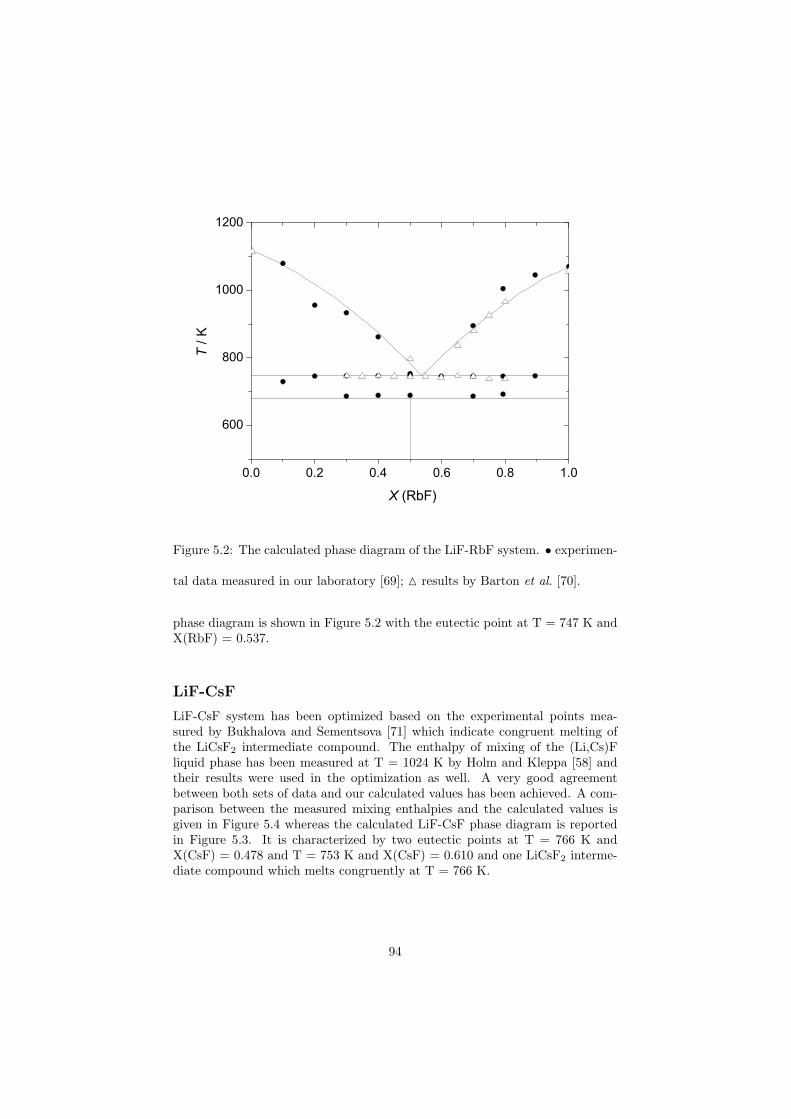
Figure 5.2: The calculated phase diagram of the LiF-RbF system. • experimen-

tal data measured in our laboratory [69]; results by Barton et al. [70].

phase diagram is shown in Figure 5.2 with the eutectic point at T = 747 K andX(RbF) = 0.537.

LiF-CsF

LiF-CsF system has been optimized based on the experimental points mea-sured by Bukhalova and Sementsova [71] which indicate congruent melting ofthe LiCsF2 intermediate compound. The enthalpy of mixing of the (Li,Cs)Fliquid phase has been measured at T = 1024 K by Holm and Kleppa [58] andtheir results were used in the optimization as well. A very good agreementbetween both sets of data and our calculated values has been achieved. A com-parison between the measured mixing enthalpies and the calculated values isgiven in Figure 5.4 whereas the calculated LiF-CsF phase diagram is reportedin Figure 5.3. It is characterized by two eutectic points at T = 766 K andX(CsF) = 0.478 and T = 753 K and X(CsF) = 0.610 and one LiCsF2 interme-diate compound which melts congruently at T = 766 K.

94

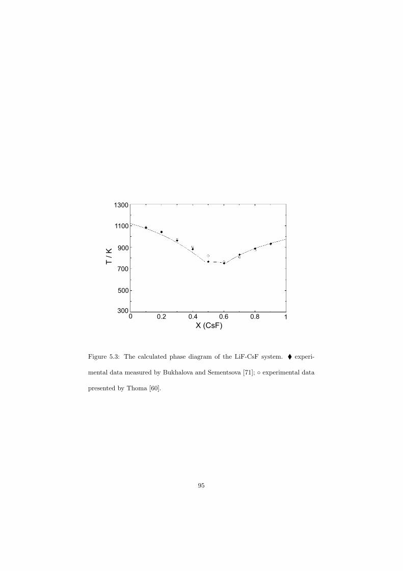
300

500

700

900

1100

1300

10 0.2 0.4 0.6 0.8

T / K

X (CsF)

Figure 5.3: The calculated phase diagram of the LiF-CsF system. experi-

mental data measured by Bukhalova and Sementsova [71]; experimental data

presented by Thoma [60].

95

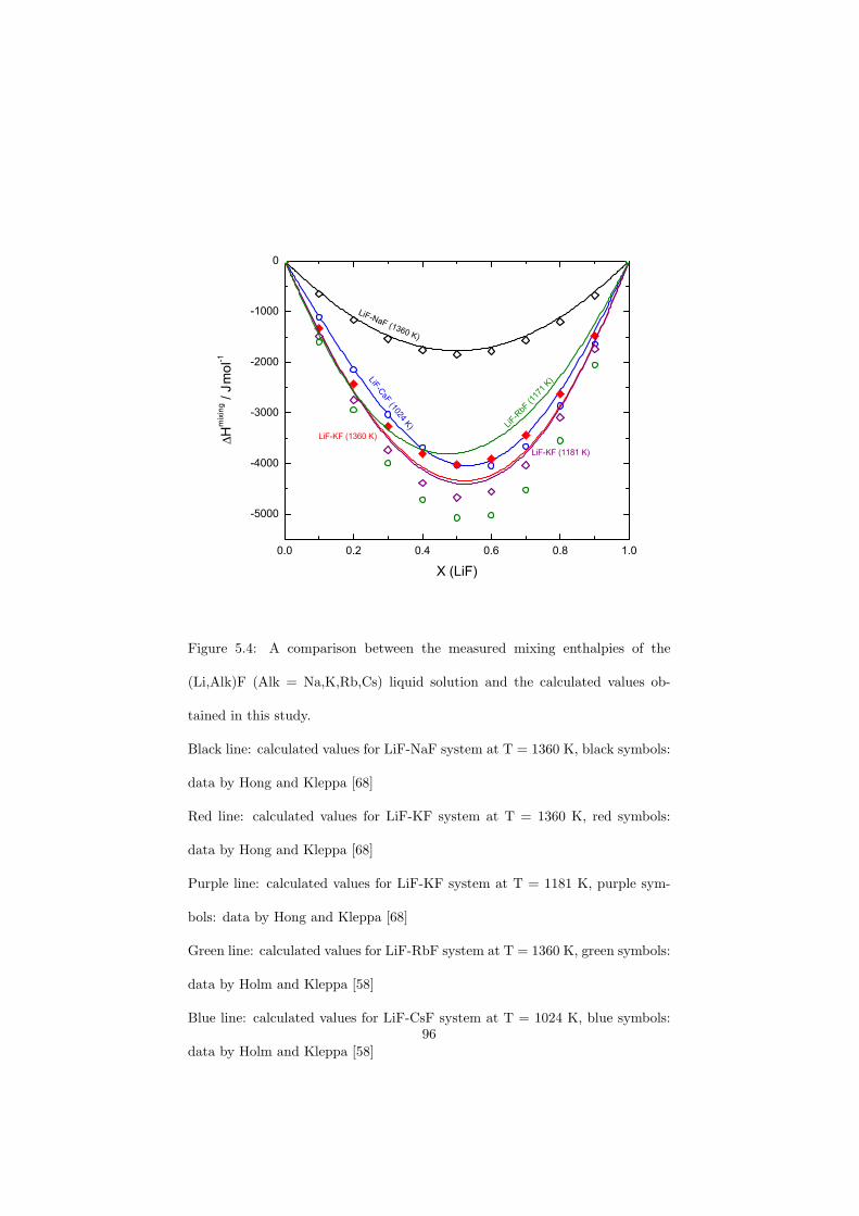
0.0 0.2 0.4 0.6 0.8 1.0

-5000

-4000

-3000

-2000

-1000

0

LiF-C

sF (1024 K

) LiF-R

bF (1

171

K)

LiF-KF (1181 K)

LiF-KF (1360 K)

∆H

mix

ing / J

. mo

l-1

X (LiF)

LiF-NaF (1360 K)

Figure 5.4: A comparison between the measured mixing enthalpies of the

(Li,Alk)F (Alk = Na,K,Rb,Cs) liquid solution and the calculated values ob-

tained in this study.

Black line: calculated values for LiF-NaF system at T = 1360 K, black symbols:

data by Hong and Kleppa [68]

Red line: calculated values for LiF-KF system at T = 1360 K, red symbols:

data by Hong and Kleppa [68]

Purple line: calculated values for LiF-KF system at T = 1181 K, purple sym-

bols: data by Hong and Kleppa [68]

Green line: calculated values for LiF-RbF system at T = 1360 K, green symbols:

data by Holm and Kleppa [58]

Blue line: calculated values for LiF-CsF system at T = 1024 K, blue symbols:

data by Holm and Kleppa [58]

96

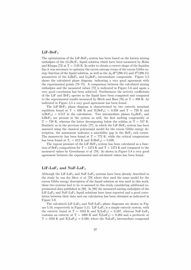
LiF-BeF2

The optimization of the LiF-BeF2 system has been based on the known mixingenthalpies of the (Li,Be)Fx liquid solution which have been measured by Holmand Kleppa [72] at T = 1135 K. In order to obtain a correct shape of the liquidusline it was necessary to optimize the excess entropy terms of the excess Gibbs en-ergy function of the liquid solution, as well as the ∆fH0(298.15) and S0(298.15)parameters of the LiBeF3 and Li2BeF4 intermediate compounds. Figure 5.5shows the calculated phase diagram, indicating a very good agreement withthe experimental points [73–75]. A comparison between the calculated mixingenthalpies and the measured values [72] is indicated in Figure 5.6 and again avery good correlation has been achieved. Furthermore the activity coefficientsof the LiF and BeF2 species in the liquid have been computed and comparedto the experimental results measured by Hitch and Baes [76] at T = 898 K. Asindicated in Figure 5.5 a very good agreement has been found.

The LiF-BeF2 phase diagram is characterized by two eutectic invariantequilibria found at T = 636 K and X(BeF2) = 0.328 and T = 729 K andx(BeF2) = 0.517 in the calculation. Two intermediate phases Li2BeF4 andLiBeF3 are present in the system as well, the first melting congruently atT = 729 K, whereas the latter decomposing below the solidus at T = 557 K.Similarly as in the previous study [77], in which the LiF-BeF2 system has beenassessed using the classical polynomial model for the excess Gibbs energy de-scription, the assessment indicates a miscibility gap in the BeF2 rich corner.The monotectic has been found at T = 772 K, while the critical temperaturehas been found at Tc = 812 K and X(BeF2) = 0.826.

The vapour pressure of the LiF-BeF2 system has been calculated as a func-tion of BeF2 composition for T = 1273 K and T = 1373 K and compared to themeasured values by Greenbaum et al. [78]. As shown in Figure 5.8 a very goodagreement between the experimental and calculated values has been found.

LiF-LaF3 and NaF-LaF3

Although the LiF-LaF3 and NaF-LaF3 systems have been already described inthe study by van der Meer et al. [79] where they used the same model for theexcess Gibbs energy description of the liquid solution as was used in this work,these two systems had to be re-assessed in this study considering additional ex-perimental data published in [80]. In [80] the measured mixing enthalpies of theLiF-LaF3 and NaF-LaF3 liquid solutions have been reported and a good corre-lation between their data and our calculation has been obtained as indicated inFigure 5.9.

The calculated LiF-LaF3 and NaF-LaF3 phase diagrams are shown in Fig-ure 5.10, respectively in Figure 5.11. LiF-LaF3 is a simple eutectic system, withthe eutectic found at T = 1043 K and X(LaF3) = 0.167, whereas NaF-LaF3

contains an eutectic at T = 1008 K and X(LaF3) = 0.283 and a peritectic atT = 1058 K and X(LaF3) = 0.338, where the NaLaF4 intermediate compound

97

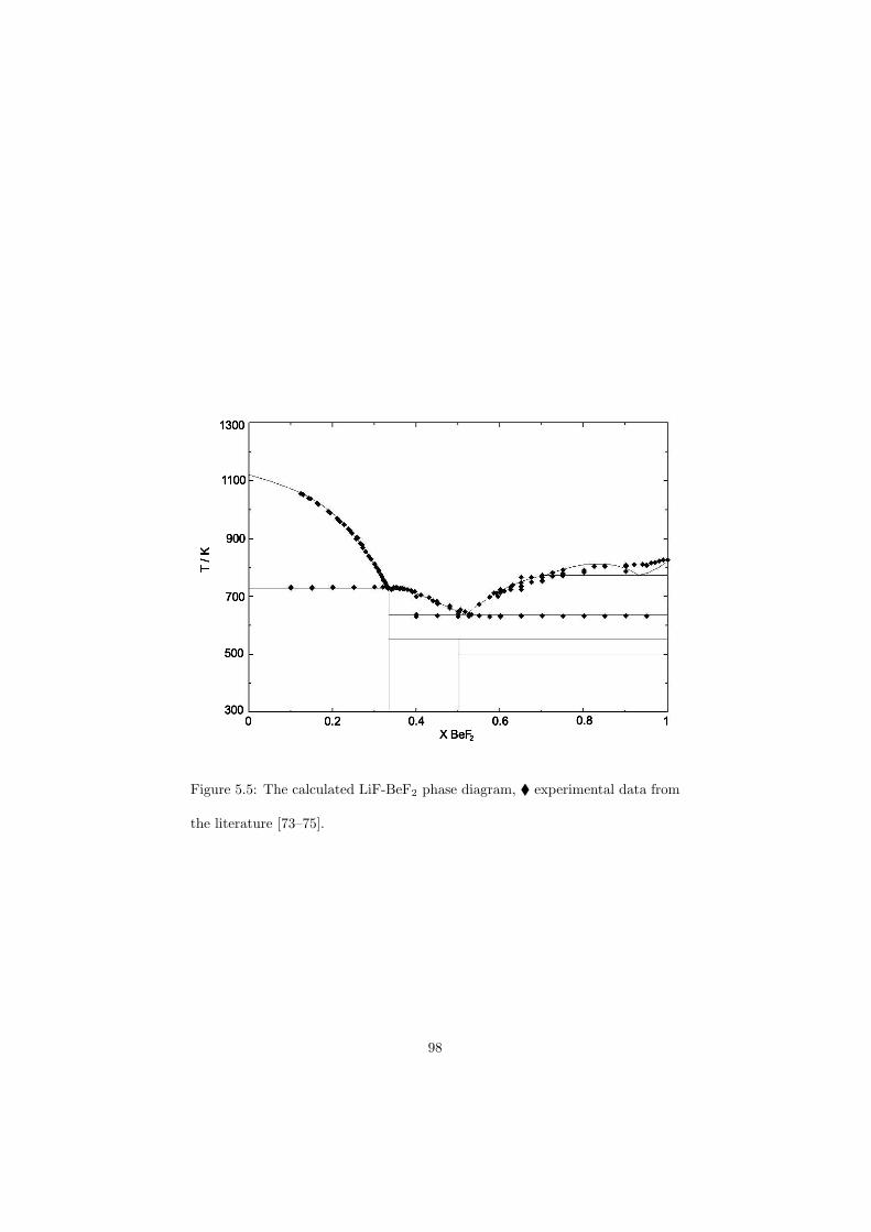
Figure 5.5: The calculated LiF-BeF2 phase diagram, experimental data from

the literature [73–75].

98

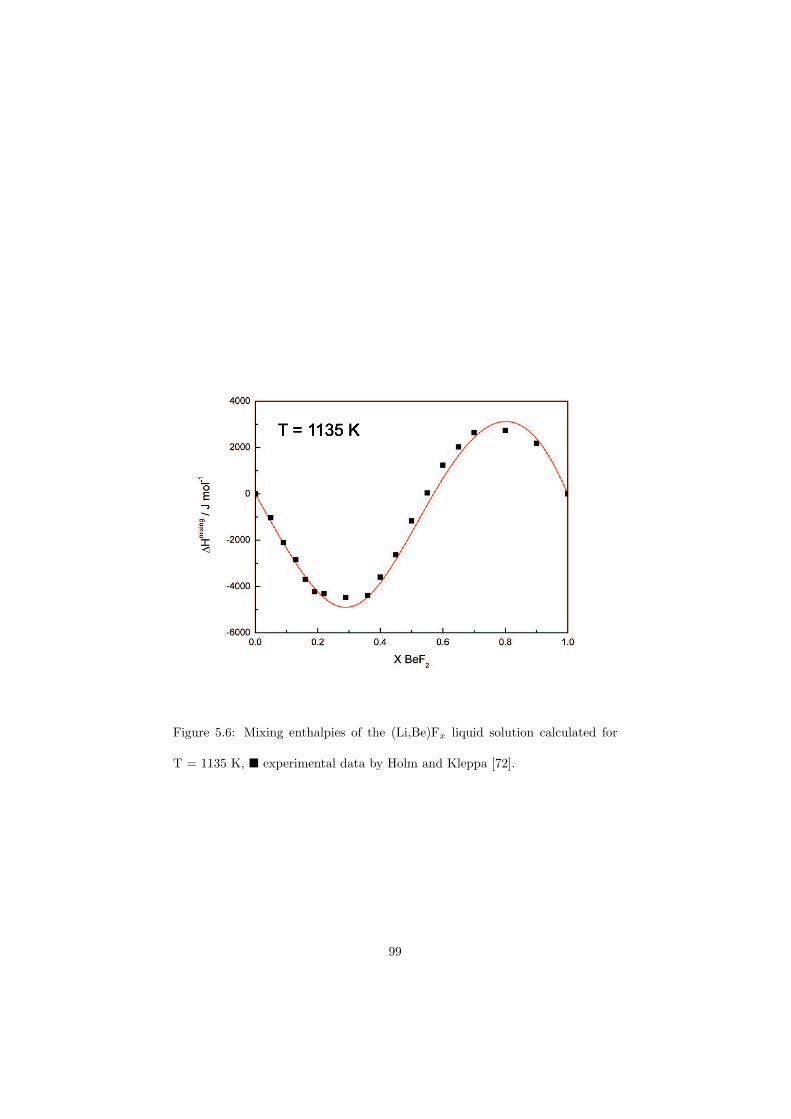
Figure 5.6: Mixing enthalpies of the (Li,Be)Fx liquid solution calculated for

T = 1135 K, experimental data by Holm and Kleppa [72].

99

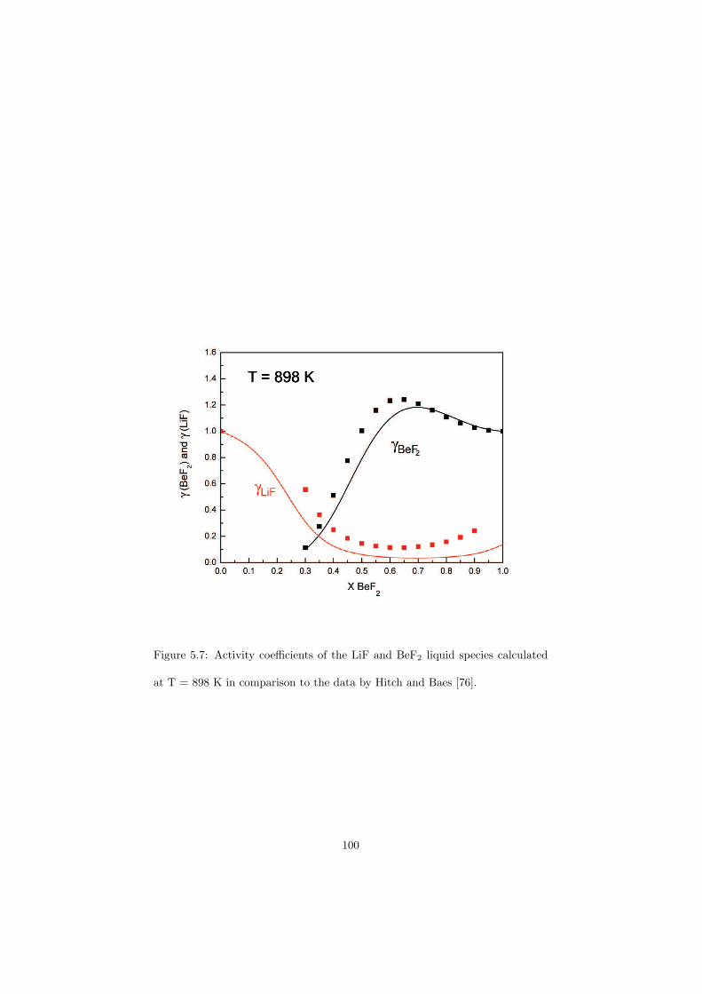
Figure 5.7: Activity coefficients of the LiF and BeF2 liquid species calculated

at T = 898 K in comparison to the data by Hitch and Baes [76].

100

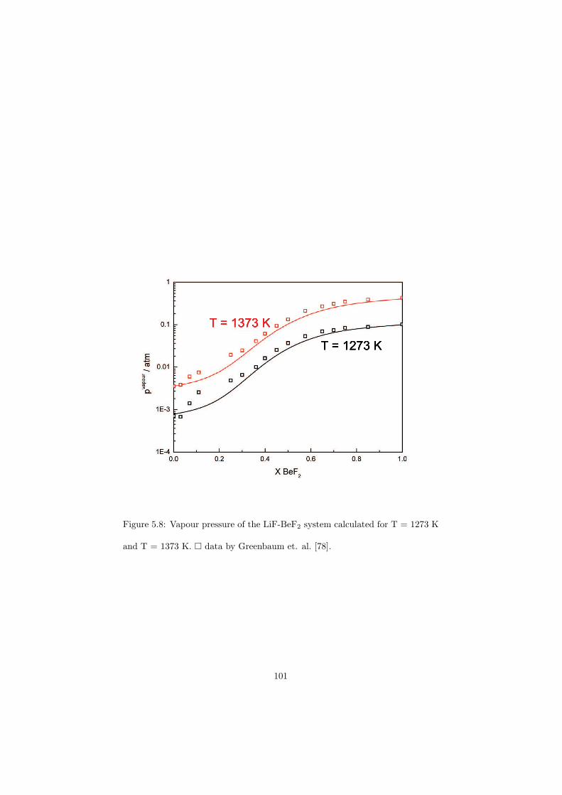
Figure 5.8: Vapour pressure of the LiF-BeF2 system calculated for T = 1273 K

and T = 1373 K. data by Greenbaum et. al. [78].

101

decomposes.

LiF-ZrF4

The LiF-ZrF4 system is among the systems optimized in this study using theclassical polynomial model for the liquid solution description. The assessment ofthe LiF-ZrF4 system was based on the experimental data measured by Thomaet al. [74, 85]. It is characterized by three eutectics and one peritectic, wherethe Li3Zr4F19 intermediate compound decomposes. The calculated values forthe eutectic points are: E1 = 882 K at X(ZrF4) = 0.192, E2 = 855 K atX(ZrF4) = 0.325 and E3 = 775 K at X(ZrF4) = 0.473, while the peritecticinvariant equilibrium corresponds to T = 798 K at X(ZrF4) = 0.51. All valuesare in excellent agreement with the experimental data. In addition to Li3Zr4F19,three other intermediate compounds have been found in the LiF-ZrF4 system.Li3ZrF7 and Li2ZrF6 melting congruently at T = 934 K and T = 856 K re-spectively, while Li4ZrF8 decomposes below the solidus line at T = 762 K. Theassessed phase diagram of the LiF-ZrF4 system is shown in figure 5.12.

LiF-PuF3

The thermodynamic assessment of the LiF-PuF3 system has been based onthe known equilibrium data measured by Barton et al. [86]. The calculatedphase diagram is reported in Figure 5.13 and a very good agreement to theexperimental data has been achieved. The system is characterized by a singleeutectic found at T = 1018 K and X(PuF3) = 0.212.

NaF-KF

The optimization of the NaF-KF system was based on the experimental datameasured by Holm [15]. It is a simple eutectic system with the eutectic atT = 991 K and X(KF) = 0.616. A limited solid solubility of NaF in KF of5.3 mole% and 0.3 mole% of KF in the NaF matrix at the eutectic temperatureappears in this system. The calculated phase diagram is shown in Figure 5.14.Holm and Kleppa [58] also measured the mixing enthalpy at T = 1281 K for aNaF/KF = 1/1 composition and found -94 J· mol−1. This is in perfect agree-ment with our value which is -87 J· mol−1.

NaF-RbF

The NaF-RbF system is a simple eutectic system with the eutectic point foundat T = 939 K and X(RbF) = 0.679. The solidus and liquidus points were

102

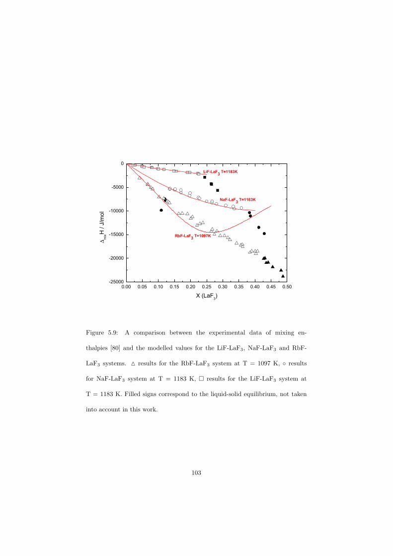
0.00 0.05 0.10 0.15 0.20 0.25 0.30 0.35 0.40 0.45 0.50-25000

-20000

-15000

-10000

-5000

0

RbF-LaF3 T=1097K

NaF-LaF3 T=1183K

∆m

ixH

/ J

/mo

l

X (LaF3)

LiF-LaF3 T=1183K

Figure 5.9: A comparison between the experimental data of mixing en-

thalpies [80] and the modelled values for the LiF-LaF3, NaF-LaF3 and RbF-

LaF3 systems. results for the RbF-LaF3 system at T = 1097 K, results

for NaF-LaF3 system at T = 1183 K, results for the LiF-LaF3 system at

T = 1183 K. Filled signs correspond to the liquid-solid equilibrium, not taken

into account in this work.

103

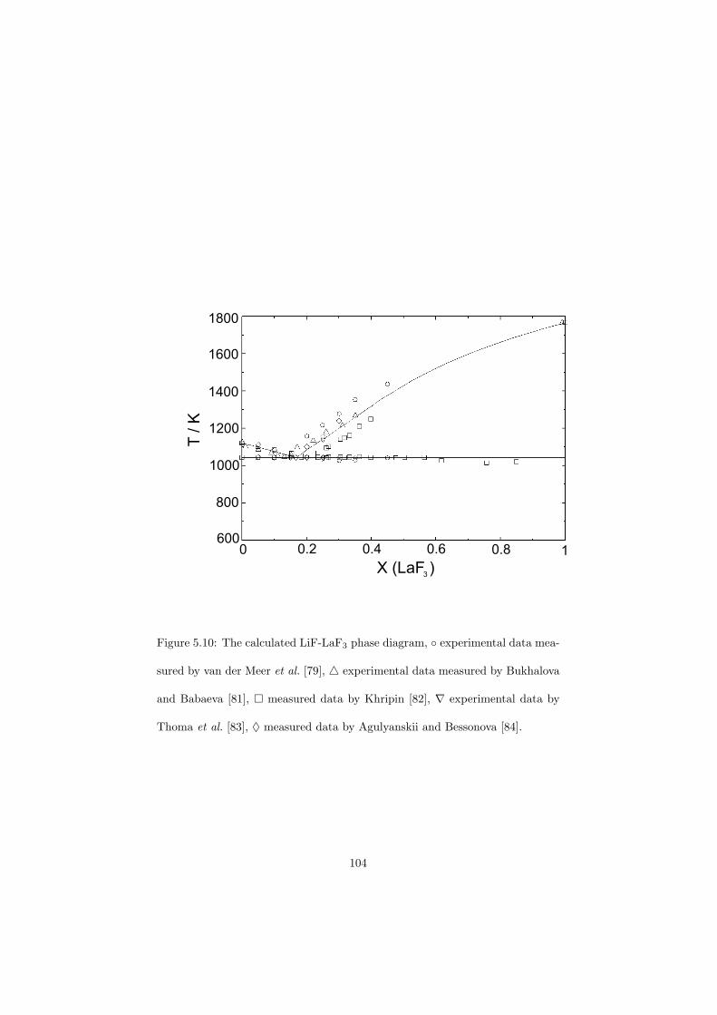
600

800

1000

1200

1400

1600

1800

T / K

0 0.2 0.4 0.6 0.8 1

X (LaF )3

Figure 5.10: The calculated LiF-LaF3 phase diagram, experimental data mea-

sured by van der Meer et al. [79], experimental data measured by Bukhalova

and Babaeva [81], measured data by Khripin [82], ∇ experimental data by

Thoma et al. [83], ♦ measured data by Agulyanskii and Bessonova [84].

104

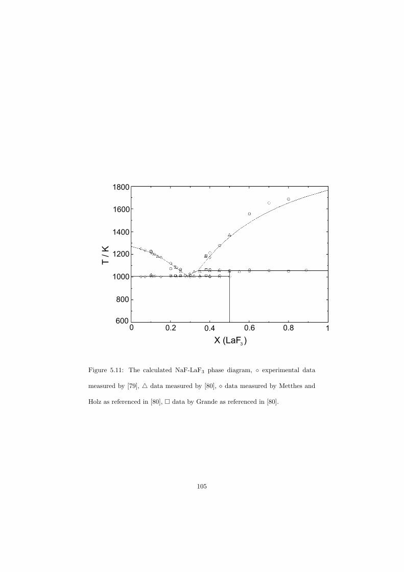
0600

800

1000

1200

1400

1600

1800

X (LaF )3

0.2 0.4 0.6 0.8 1

T / K

Figure 5.11: The calculated NaF-LaF3 phase diagram, experimental data

measured by [79], data measured by [80], ⋄ data measured by Metthes and

Holz as referenced in [80], data by Grande as referenced in [80].

105

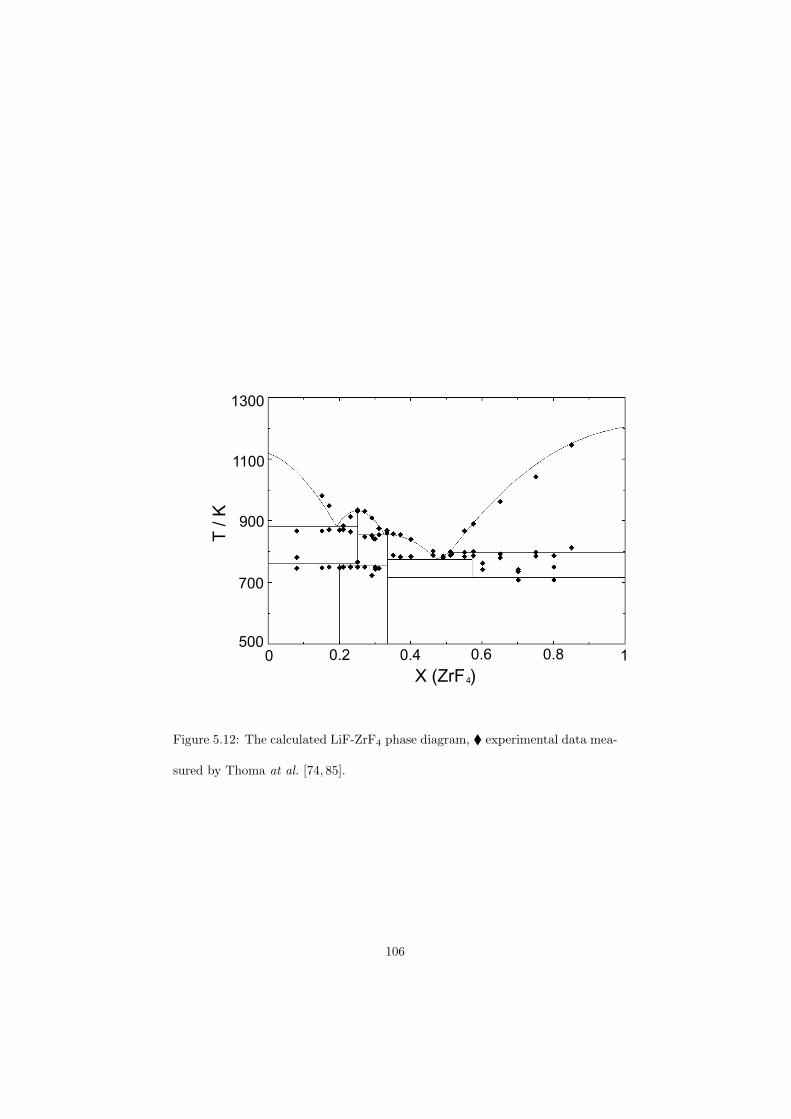
500

700

900

1100

1300

0 0.2 0.60.4 0.8 1

T / K

X (ZrF )4

Figure 5.12: The calculated LiF-ZrF4 phase diagram, experimental data mea-

sured by Thoma at al. [74, 85].

106

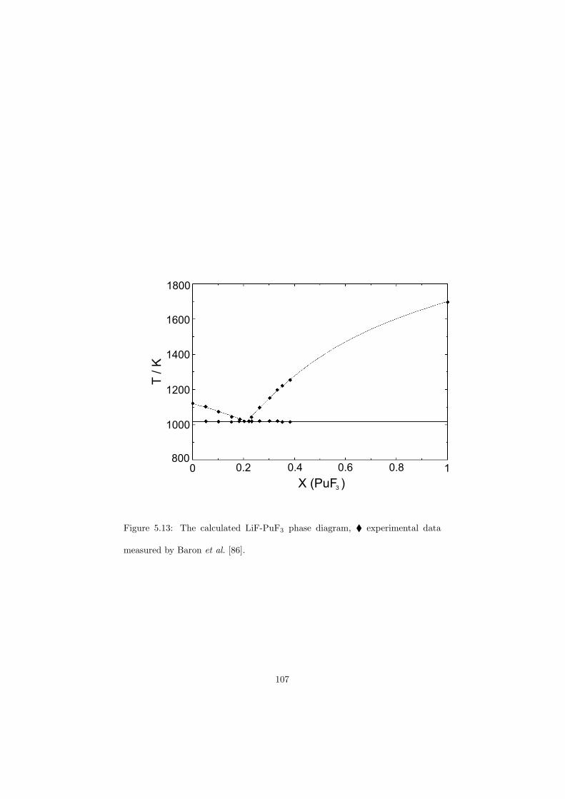
800

1000

1200

1400

1600

1800

0 0.2 0.4 0.6 0.8 1

T / K

X (PuF )3

Figure 5.13: The calculated LiF-PuF3 phase diagram, experimental data

measured by Baron et al. [86].

107

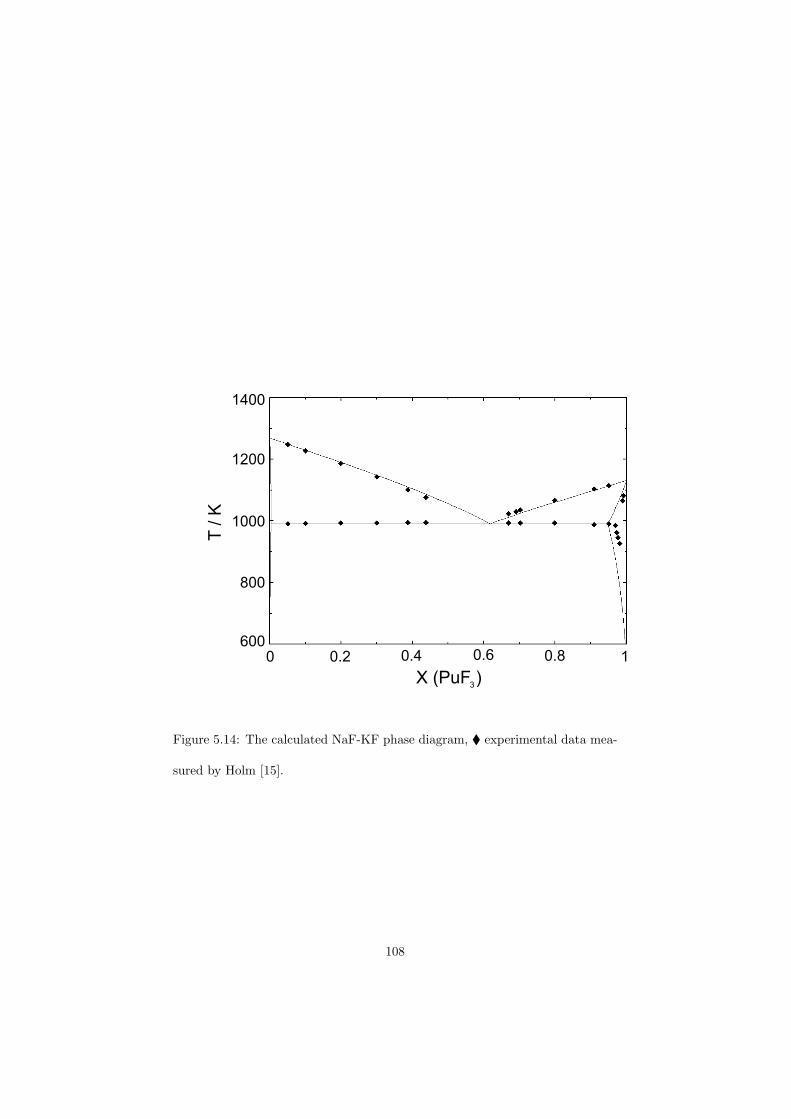
600

800

1400

1200

1000

0 0.2 0.4 0.6 0.8 1

X (PuF )3

T / K

Figure 5.14: The calculated NaF-KF phase diagram, experimental data mea-

sured by Holm [15].

108

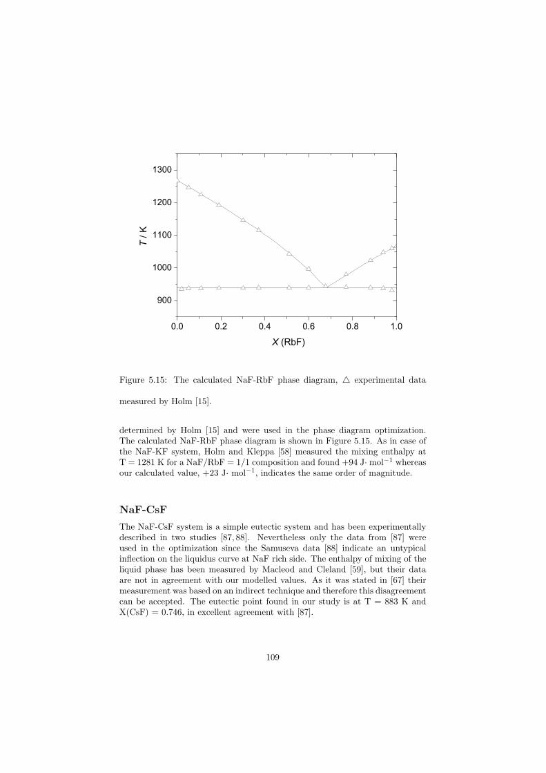
Figure 5.15: The calculated NaF-RbF phase diagram, experimental data

measured by Holm [15].

determined by Holm [15] and were used in the phase diagram optimization.The calculated NaF-RbF phase diagram is shown in Figure 5.15. As in case ofthe NaF-KF system, Holm and Kleppa [58] measured the mixing enthalpy atT = 1281 K for a NaF/RbF = 1/1 composition and found +94 J· mol−1 whereasour calculated value, +23 J· mol−1, indicates the same order of magnitude.

NaF-CsF

The NaF-CsF system is a simple eutectic system and has been experimentallydescribed in two studies [87, 88]. Nevertheless only the data from [87] wereused in the optimization since the Samuseva data [88] indicate an untypicalinflection on the liquidus curve at NaF rich side. The enthalpy of mixing of theliquid phase has been measured by Macleod and Cleland [59], but their dataare not in agreement with our modelled values. As it was stated in [67] theirmeasurement was based on an indirect technique and therefore this disagreementcan be accepted. The eutectic point found in our study is at T = 883 K andX(CsF) = 0.746, in excellent agreement with [87].

109

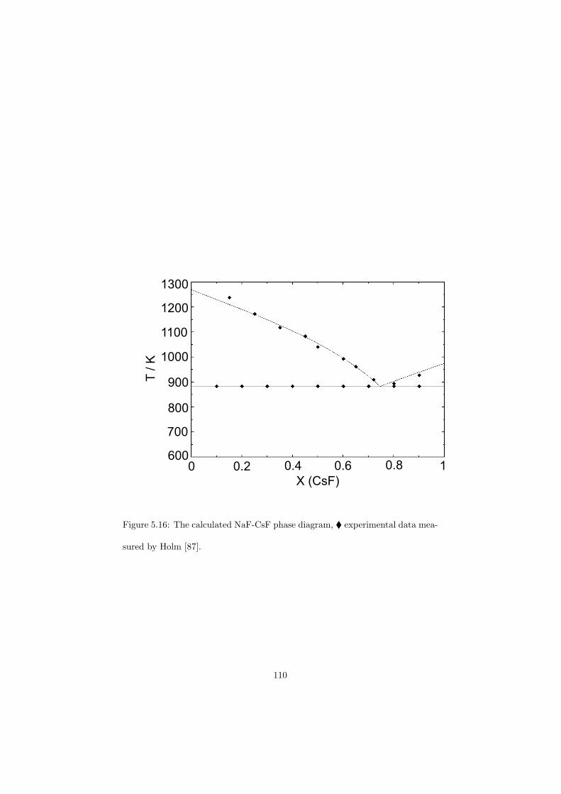
600

900

800

700

1300

1200

1100

1000

0 0.2 10.80.60.4

X (CsF)

T / K

Figure 5.16: The calculated NaF-CsF phase diagram, experimental data mea-

sured by Holm [87].

110

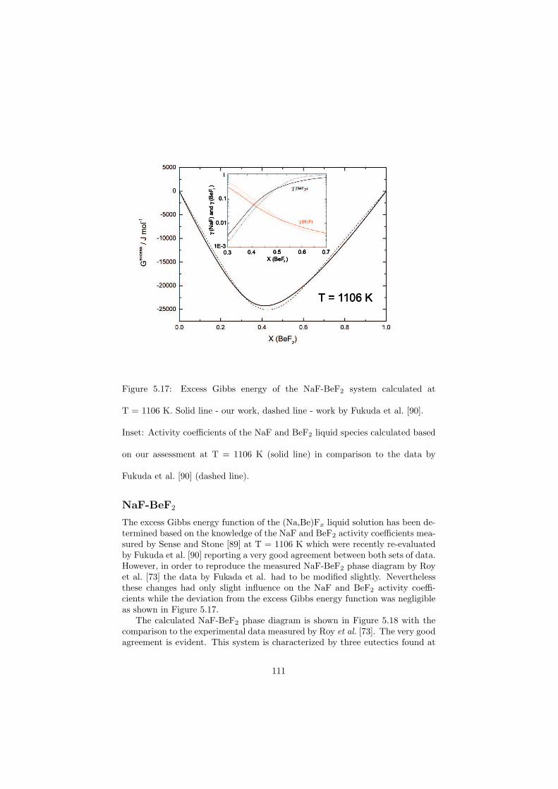
Figure 5.17: Excess Gibbs energy of the NaF-BeF2 system calculated at

T = 1106 K. Solid line - our work, dashed line - work by Fukuda et al. [90].

Inset: Activity coefficients of the NaF and BeF2 liquid species calculated based

on our assessment at T = 1106 K (solid line) in comparison to the data by

Fukuda et al. [90] (dashed line).

NaF-BeF2

The excess Gibbs energy function of the (Na,Be)Fx liquid solution has been de-termined based on the knowledge of the NaF and BeF2 activity coefficients mea-sured by Sense and Stone [89] at T = 1106 K which were recently re-evaluatedby Fukuda et al. [90] reporting a very good agreement between both sets of data.However, in order to reproduce the measured NaF-BeF2 phase diagram by Royet al. [73] the data by Fukada et al. had to be modified slightly. Neverthelessthese changes had only slight influence on the NaF and BeF2 activity coeffi-cients while the deviation from the excess Gibbs energy function was negligibleas shown in Figure 5.17.

The calculated NaF-BeF2 phase diagram is shown in Figure 5.18 with thecomparison to the experimental data measured by Roy et al. [73]. The very goodagreement is evident. This system is characterized by three eutectics found at

111

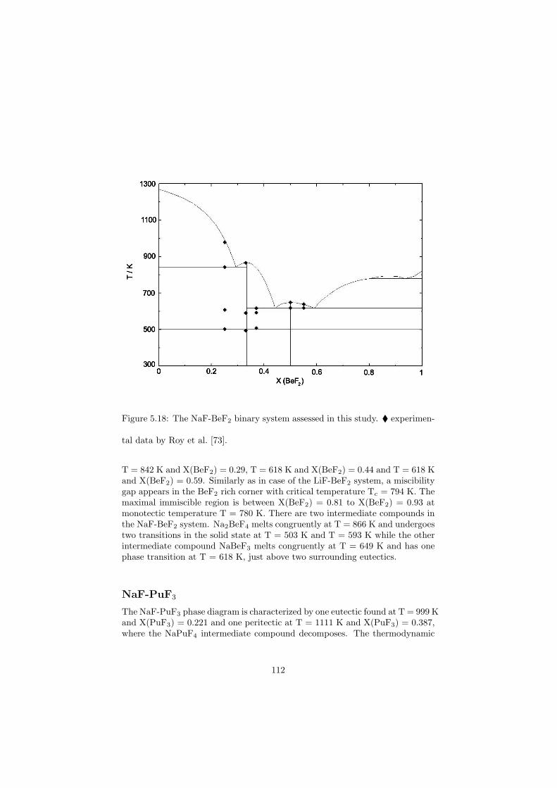
Figure 5.18: The NaF-BeF2 binary system assessed in this study. experimen-

tal data by Roy et al. [73].

T = 842 K and X(BeF2) = 0.29, T = 618 K and X(BeF2) = 0.44 and T = 618 Kand X(BeF2) = 0.59. Similarly as in case of the LiF-BeF2 system, a miscibilitygap appears in the BeF2 rich corner with critical temperature Tc = 794 K. Themaximal immiscible region is between X(BeF2) = 0.81 to X(BeF2) = 0.93 atmonotectic temperature T = 780 K. There are two intermediate compounds inthe NaF-BeF2 system. Na2BeF4 melts congruently at T = 866 K and undergoestwo transitions in the solid state at T = 503 K and T = 593 K while the otherintermediate compound NaBeF3 melts congruently at T = 649 K and has onephase transition at T = 618 K, just above two surrounding eutectics.

NaF-PuF3

The NaF-PuF3 phase diagram is characterized by one eutectic found at T = 999 Kand X(PuF3) = 0.221 and one peritectic at T = 1111 K and X(PuF3) = 0.387,where the NaPuF4 intermediate compound decomposes. The thermodynamic

112

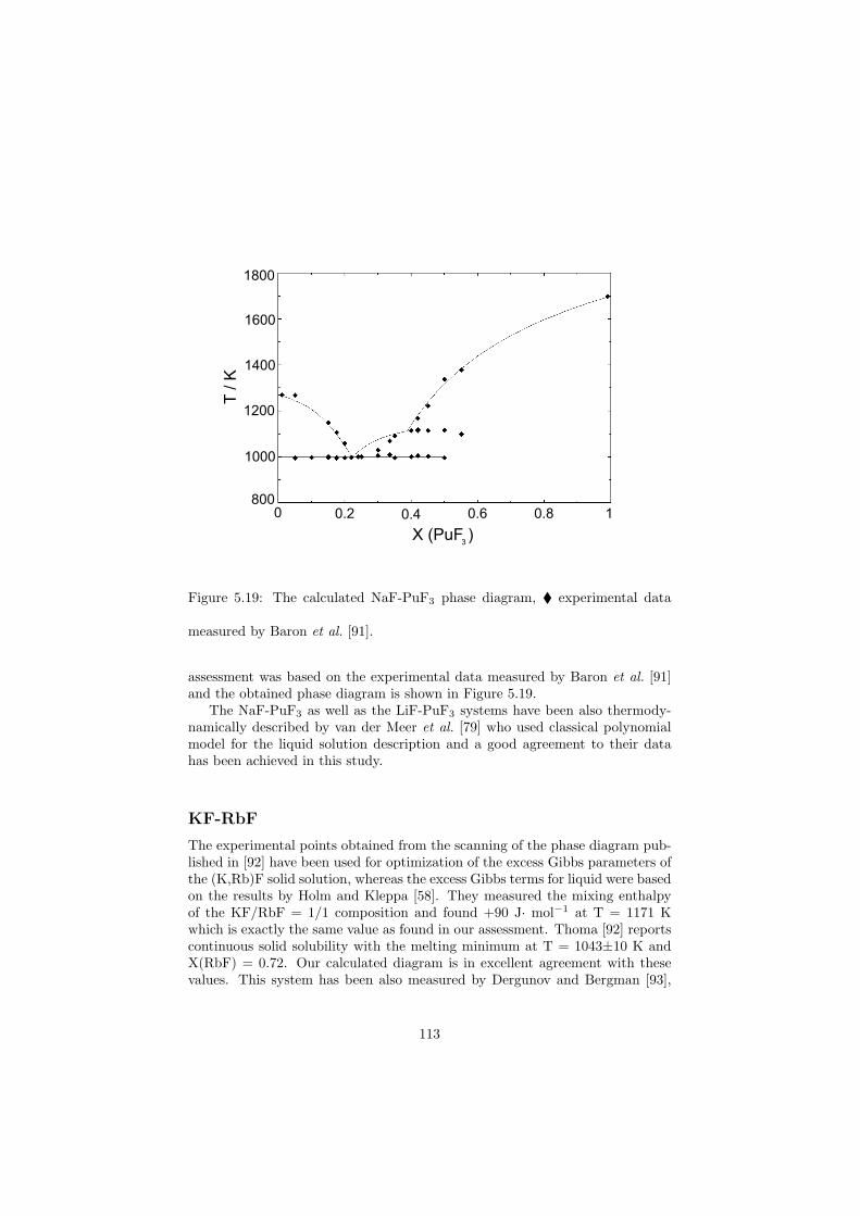
800

1000

1200

1400

1600

1800

0 0.2 0.4 0.6 0.8 1

X (PuF )3

T / K

Figure 5.19: The calculated NaF-PuF3 phase diagram, experimental data

measured by Baron et al. [91].

assessment was based on the experimental data measured by Baron et al. [91]and the obtained phase diagram is shown in Figure 5.19.

The NaF-PuF3 as well as the LiF-PuF3 systems have been also thermody-namically described by van der Meer et al. [79] who used classical polynomialmodel for the liquid solution description and a good agreement to their datahas been achieved in this study.

KF-RbF

The experimental points obtained from the scanning of the phase diagram pub-lished in [92] have been used for optimization of the excess Gibbs parameters ofthe (K,Rb)F solid solution, whereas the excess Gibbs terms for liquid were basedon the results by Holm and Kleppa [58]. They measured the mixing enthalpyof the KF/RbF = 1/1 composition and found +90 J· mol−1 at T = 1171 Kwhich is exactly the same value as found in our assessment. Thoma [92] reportscontinuous solid solubility with the melting minimum at T = 1043±10 K andX(RbF) = 0.72. Our calculated diagram is in excellent agreement with thesevalues. This system has been also measured by Dergunov and Bergman [93],

113

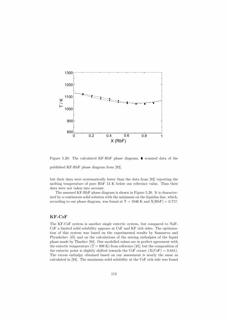
800

1000

900

1300

1200

1100

0 10.2 0.4 0.6 0.8

T / K

X (RbF)

Figure 5.20: The calculated KF-RbF phase diagram, scanned data of the

published KF-RbF phase diagram from [92].

but their data were systematically lower than the data from [92] reporting themelting temperature of pure RbF 13 K below our reference value. Thus theirdata were not taken into account.

The assessed KF-RbF phase diagram is shown in Figure 5.20. It is character-ized by a continuous solid solution with the minimum on the liquidus line, which,according to our phase diagram, was found at T = 1046 K and X(RbF) = 0.717.

KF-CsF

The KF-CsF system is another single eutectic system, but compared to NaF-CsF a limited solid solubility appears at CsF and KF rich sides. The optimiza-tion of this system was based on the experimental results by Samuseva andPlyushchev [45] and on the calculations of the mixing enthalpies of the liquidphase made by Tkachev [94]. Our modelled values are in perfect agreement withthe eutectic temperature (T = 898 K) from reference [45], but the composition ofthe eutectic point is slightly shifted towards the CsF corner (X(CsF) = 0.641).The excess enthalpy obtained based on our assessment is nearly the same ascalculated in [94]. The maximum solid solubility at the CsF rich side was found

114

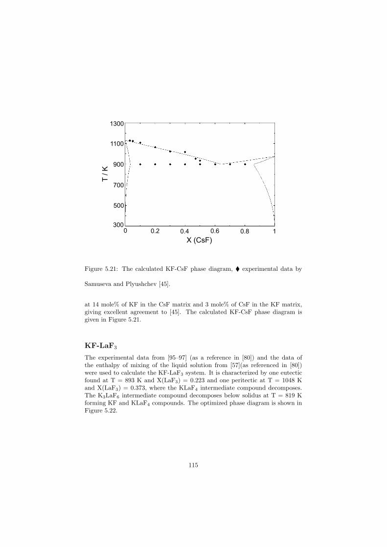
300

500

700

900

1100

1300

0 10.80.60.40.2

X (CsF)

T / K

Figure 5.21: The calculated KF-CsF phase diagram, experimental data by

Samuseva and Plyushchev [45].

at 14 mole% of KF in the CsF matrix and 3 mole% of CsF in the KF matrix,giving excellent agreement to [45]. The calculated KF-CsF phase diagram isgiven in Figure 5.21.

KF-LaF3

The experimental data from [95–97] (as a reference in [80]) and the data ofthe enthalpy of mixing of the liquid solution from [57](as referenced in [80])were used to calculate the KF-LaF3 system. It is characterized by one eutecticfound at T = 893 K and X(LaF3) = 0.223 and one peritectic at T = 1048 Kand X(LaF3) = 0.373, where the KLaF4 intermediate compound decomposes.The K3LaF6 intermediate compound decomposes below solidus at T = 819 Kforming KF and KLaF4 compounds. The optimized phase diagram is shown inFigure 5.22.

115

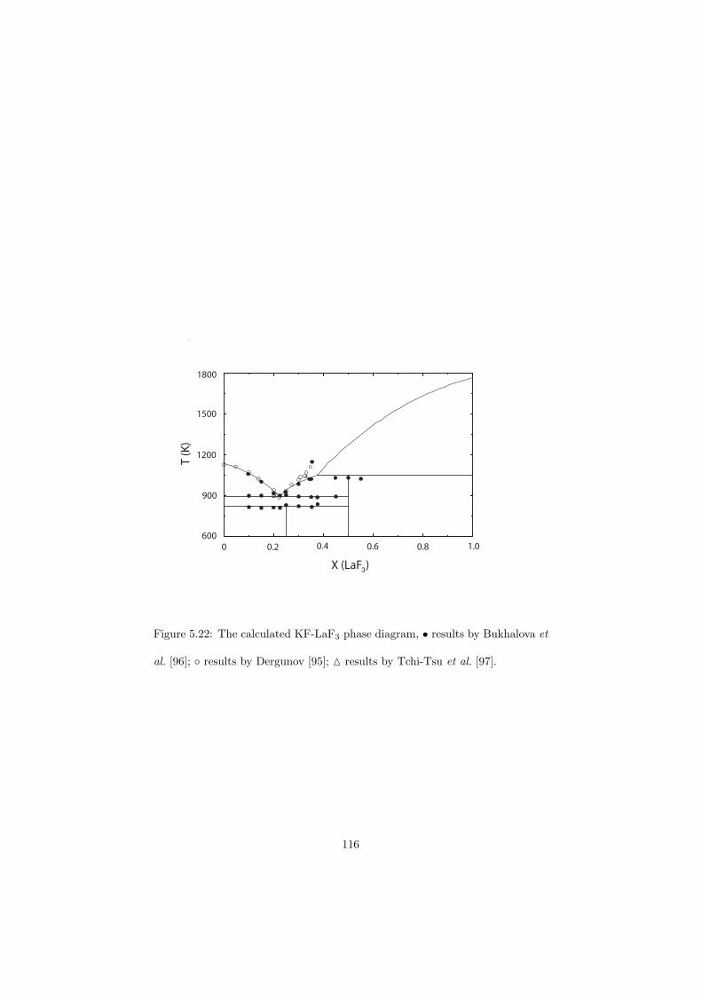
mole LaF3/(KF+LaF3)

T(K

)

0 .2 .4 .6 .8 1

600

900

1200

1500

1800

600

900

1200

1500

1800

0 0.2 0.4 0.6 0.8 1.0

X (LaF )

T (

K)

3

Figure 5.22: The calculated KF-LaF3 phase diagram, • results by Bukhalova et

al. [96]; results by Dergunov [95]; results by Tchi-Tsu et al. [97].

116

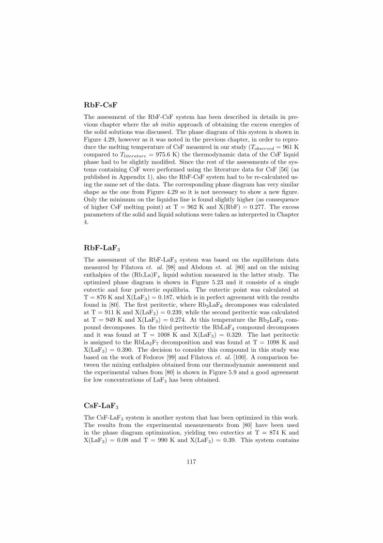
RbF-CsF

The assessment of the RbF-CsF system has been described in details in pre-vious chapter where the ab initio approach of obtaining the excess energies ofthe solid solutions was discussed. The phase diagram of this system is shown inFigure 4.29, however as it was noted in the previous chapter, in order to repro-duce the melting temperature of CsF measured in our study (Tobserved = 961 Kcompared to Tliterature = 975.6 K) the thermodynamic data of the CsF liquidphase had to be slightly modified. Since the rest of the assessments of the sys-tems containing CsF were performed using the literature data for CsF [56] (aspublished in Appendix 1), also the RbF-CsF system had to be re-calculated us-ing the same set of the data. The corresponding phase diagram has very similarshape as the one from Figure 4.29 so it is not necessary to show a new figure.Only the minimum on the liquidus line is found slightly higher (as consequenceof higher CsF melting point) at T = 962 K and X(RbF) = 0.277. The excessparameters of the solid and liquid solutions were taken as interpreted in Chapter4.

RbF-LaF3

The assessment of the RbF-LaF3 system was based on the equilibrium datameasured by Filatova et. al. [98] and Abdoun et. al. [80] and on the mixingenthalpies of the (Rb,La)Fx liquid solution measured in the latter study. Theoptimized phase diagram is shown in Figure 5.23 and it consists of a singleeutectic and four peritectic equilibria. The eutectic point was calculated atT = 876 K and X(LaF3) = 0.187, which is in perfect agreement with the resultsfound in [80]. The first peritectic, where Rb3LaF6 decomposes was calculatedat T = 911 K and X(LaF3) = 0.239, while the second peritectic was calculatedat T = 949 K and X(LaF3) = 0.274. At this temperature the Rb2LaF6 com-pound decomposes. In the third peritectic the RbLaF4 compound decomposesand it was found at T = 1008 K and X(LaF3) = 0.329. The last peritecticis assigned to the RbLa2F7 decomposition and was found at T = 1098 K andX(LaF3) = 0.390. The decision to consider this compound in this study wasbased on the work of Fedorov [99] and Filatova et. al. [100]. A comparison be-tween the mixing enthalpies obtained from our thermodynamic assessment andthe experimental values from [80] is shown in Figure 5.9 and a good agreementfor low concentrations of LaF3 has been obtained.

CsF-LaF3

The CsF-LaF3 system is another system that has been optimized in this work.The results from the experimental measurements from [80] have been usedin the phase diagram optimization, yielding two eutectics at T = 874 K andX(LaF3) = 0.08 and T = 990 K and X(LaF3) = 0.39. This system contains

117

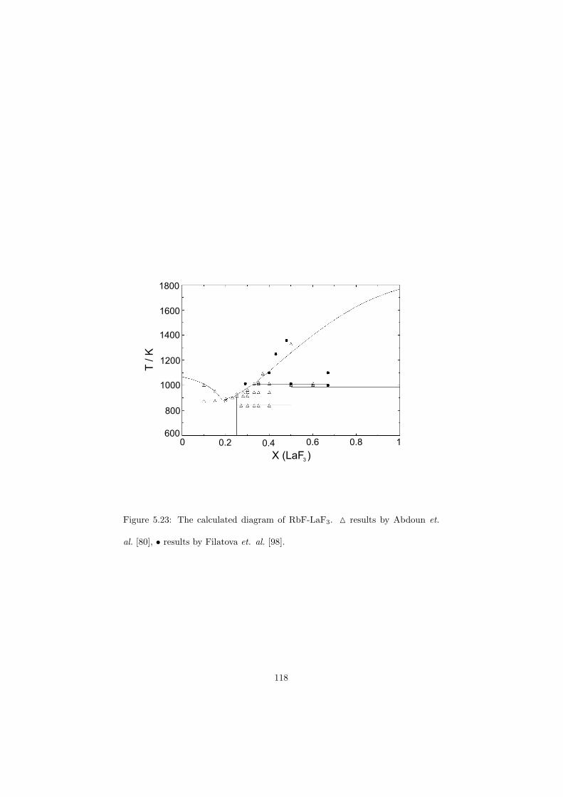
800

600

1000

1200

1400

1600

1800

0 0.2 0.4 0.6 0.8 1

X (LaF )

T / K

3

Figure 5.23: The calculated diagram of RbF-LaF3. results by Abdoun et.

al. [80], • results by Filatova et. al. [98].

118

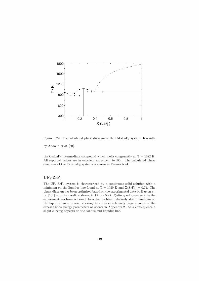
300

600

900

1200

1800

1500

0 10.60.40.2 0.8

T / K

X (LaF )3

Figure 5.24: The calculated phase diagram of the CsF-LaF3 system. results

by Abdoun et al. [80].

the Cs3LaF6 intermediate compound which melts congruently at T = 1082 K.All reported values are in excellent agreement to [80]. The calculated phasediagrams of the CsF-LaF3 systems is shown in Figures 5.24.

UF4-ZrF4

The UF4-ZrF4 system is characterized by a continuous solid solution with aminimum on the liquidus line found at T = 1039 K and X(ZrF4) = 0.71. Thephase diagram has been optimized based on the experimental data by Barton et.al. [101] and the result is shown in Figure 5.25. Quite good agreement to theexperiment has been achieved. In order to obtain relatively sharp minimum onthe liquidus curve it was necessary to consider relatively large amount of theexcess Gibbs energy parameters as shown in Appendix 2. As a consequence aslight curving appears on the solidus and liquidus line.

119

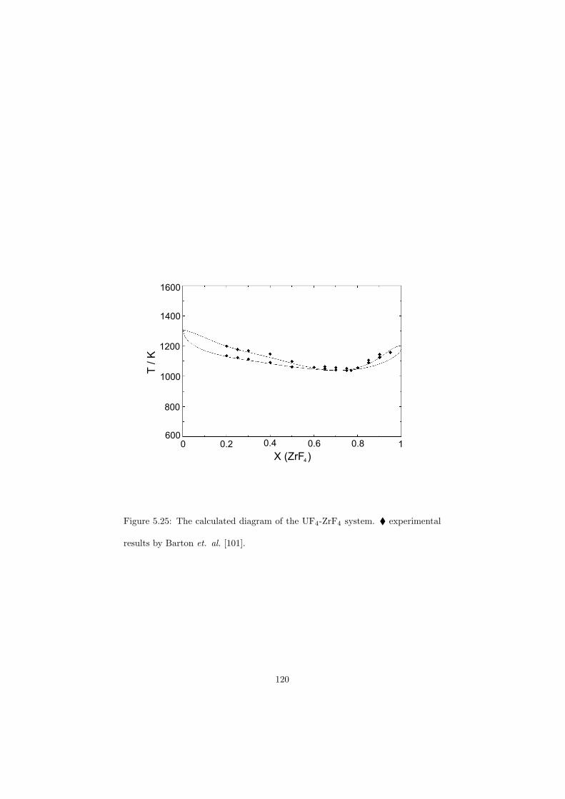
600

800

1000

1200

1400

1600

0 10.2 0.4 0.6 0.8

T / K

X (ZrF )4

Figure 5.25: The calculated diagram of the UF4-ZrF4 system. experimental

results by Barton et. al. [101].

120

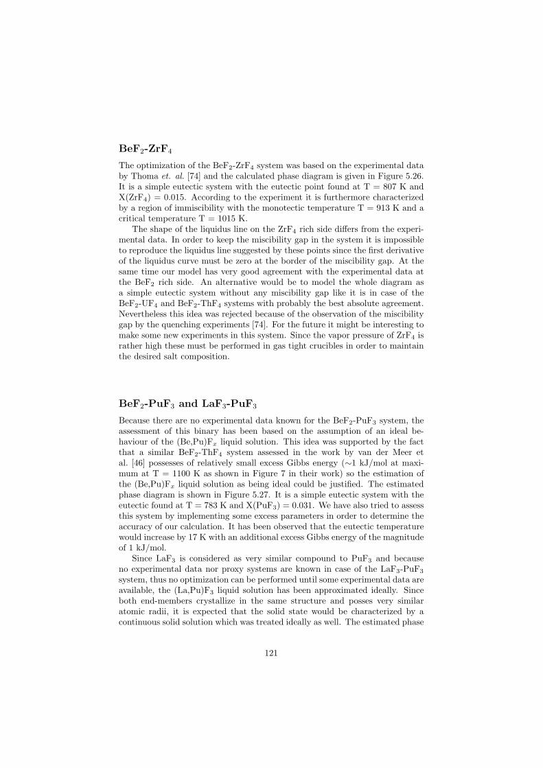
BeF2-ZrF4

The optimization of the BeF2-ZrF4 system was based on the experimental databy Thoma et. al. [74] and the calculated phase diagram is given in Figure 5.26.It is a simple eutectic system with the eutectic point found at T = 807 K andX(ZrF4) = 0.015. According to the experiment it is furthermore characterizedby a region of immiscibility with the monotectic temperature T = 913 K and acritical temperature T = 1015 K.

The shape of the liquidus line on the ZrF4 rich side differs from the experi-mental data. In order to keep the miscibility gap in the system it is impossibleto reproduce the liquidus line suggested by these points since the first derivativeof the liquidus curve must be zero at the border of the miscibility gap. At thesame time our model has very good agreement with the experimental data atthe BeF2 rich side. An alternative would be to model the whole diagram asa simple eutectic system without any miscibility gap like it is in case of theBeF2-UF4 and BeF2-ThF4 systems with probably the best absolute agreement.Nevertheless this idea was rejected because of the observation of the miscibilitygap by the quenching experiments [74]. For the future it might be interesting tomake some new experiments in this system. Since the vapor pressure of ZrF4 israther high these must be performed in gas tight crucibles in order to maintainthe desired salt composition.

BeF2-PuF3 and LaF3-PuF3

Because there are no experimental data known for the BeF2-PuF3 system, theassessment of this binary has been based on the assumption of an ideal be-haviour of the (Be,Pu)Fx liquid solution. This idea was supported by the factthat a similar BeF2-ThF4 system assessed in the work by van der Meer etal. [46] possesses of relatively small excess Gibbs energy (∼1 kJ/mol at maxi-mum at T = 1100 K as shown in Figure 7 in their work) so the estimation ofthe (Be,Pu)Fx liquid solution as being ideal could be justified. The estimatedphase diagram is shown in Figure 5.27. It is a simple eutectic system with theeutectic found at T = 783 K and X(PuF3) = 0.031. We have also tried to assessthis system by implementing some excess parameters in order to determine theaccuracy of our calculation. It has been observed that the eutectic temperaturewould increase by 17 K with an additional excess Gibbs energy of the magnitudeof 1 kJ/mol.

Since LaF3 is considered as very similar compound to PuF3 and becauseno experimental data nor proxy systems are known in case of the LaF3-PuF3

system, thus no optimization can be performed until some experimental data areavailable, the (La,Pu)F3 liquid solution has been approximated ideally. Sinceboth end-members crystallize in the same structure and posses very similaratomic radii, it is expected that the solid state would be characterized by acontinuous solid solution which was treated ideally as well. The estimated phase

121

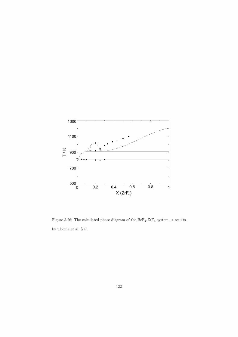
500

900

700

1300

1100

0 10.2 0.4 0.6 0.8

T / K

X (ZrF )4

Figure 5.26: The calculated phase diagram of the BeF2-ZrF4 system. results

by Thoma et al. [74].

122

300

900

600

1500

1200

1800

0 10.40.2 0.6 0.8

T / K

X (PuF )3

Figure 5.27: The estimated BeF2-PuF3 phase diagram.

diagram of the LaF3-PuF3 system is shown in Figure 5.28 and is characterizedwith a narrow two-phase field between the solidus and liquidus line with noextreme observed.

KF-PuF3, RbF-PuF3 and CsF-PuF3

Similarly as in case of the previously discussed BeF2-PuF3 and LaF3-PuF3 phasediagrams, there are no experimental data known for the KF-PuF3, RbF-PuF3

and CsF-PuF3 binary systems. Hence the optimization of these phase diagramsis impossible. Unfortunately the end-member pairs from these three systemsare chemically different with no such similarities as in case of the BeF2-PuF3 orLaF3-PuF3 phase diagrams, so the ideal approximation is not a good solution.However it is possible to profit from the chemical similarity of the LaF3 andPuF3 compounds and calculate the PuF3 containing systems using the sameexcess Gibbs parameters for the liquid solutions as obtained from the systemscontaining LaF3. For instance the excess Gibbs parameters for the KF-PuF3

liquid solution were obtained from the ones of the KF-LaF3 system.This method is only a rough approximation of the phase diagrams, but until

some experimental data are known, it is probably the best way to estimate thesesystems. Since the LiF-LaF3, NaF-LaF3, LiF-PuF3 and NaF-PuF3 systems have

123

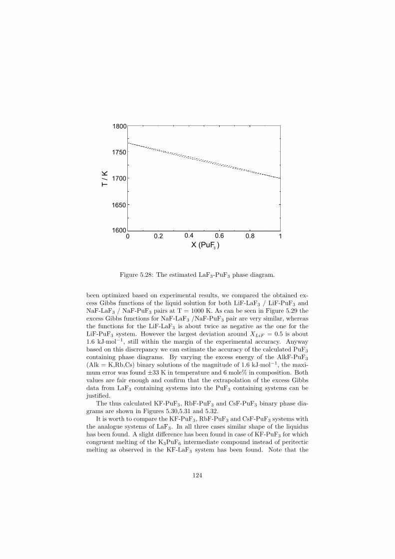
1600

1700

1800

1750

1650

0 0.2 0.8 10.60.4

T / K

X (PuF )3

Figure 5.28: The estimated LaF3-PuF3 phase diagram.

been optimized based on experimental results, we compared the obtained ex-cess Gibbs functions of the liquid solution for both LiF-LaF3 / LiF-PuF3 andNaF-LaF3 / NaF-PuF3 pairs at T = 1000 K. As can be seen in Figure 5.29 theexcess Gibbs functions for NaF-LaF3 /NaF-PuF3 pair are very similar, whereasthe functions for the LiF-LaF3 is about twice as negative as the one for theLiF-PuF3 system. However the largest deviation around XLiF = 0.5 is about1.6 kJ·mol−1, still within the margin of the experimental accuracy. Anywaybased on this discrepancy we can estimate the accuracy of the calculated PuF3

containing phase diagrams. By varying the excess energy of the AlkF-PuF3

(Alk = K,Rb,Cs) binary solutions of the magnitude of 1.6 kJ·mol−1, the maxi-mum error was found ±33 K in temperature and 6 mole% in composition. Bothvalues are fair enough and confirm that the extrapolation of the excess Gibbsdata from LaF3 containing systems into the PuF3 containing systems can bejustified.

The thus calculated KF-PuF3, RbF-PuF3 and CsF-PuF3 binary phase dia-grams are shown in Figures 5.30,5.31 and 5.32.

It is worth to compare the KF-PuF3, RbF-PuF3 and CsF-PuF3 systems withthe analogue systems of LaF3. In all three cases similar shape of the liquidushas been found. A slight difference has been found in case of KF-PuF3 for whichcongruent melting of the K3PuF6 intermediate compound instead of peritecticmelting as observed in the KF-LaF3 system has been found. Note that the

124

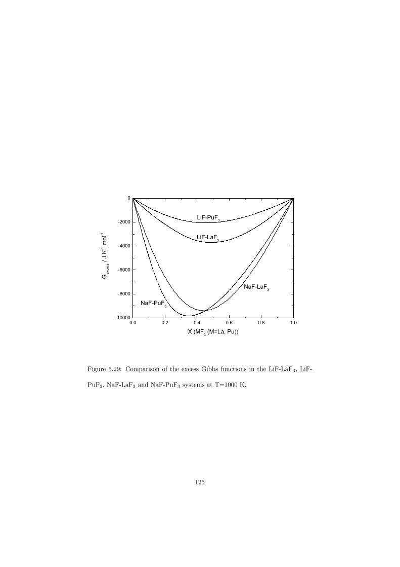
0.0 0.2 0.4 0.6 0.8 1.0-10000

-8000

-6000

-4000

-2000

0

NaF-LaF3

NaF-PuF3

LiF-LaF3

Ge

xce

ss / J

K-1 m

ol-1

X (MF3 (M=La, Pu))

LiF-PuF3

Figure 5.29: Comparison of the excess Gibbs functions in the LiF-LaF3, LiF-

PuF3, NaF-LaF3 and NaF-PuF3 systems at T=1000 K.

125

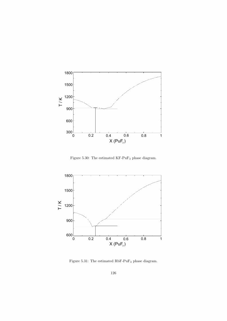
300

900

600

1500

1200

1800

0 0.4 0.60.2 0.8 1

T / K

X (PuF )3

Figure 5.30: The estimated KF-PuF3 phase diagram.

600

900

1200

1500

1800

0 0.2 0.4 0.6 0.8 1

3X (PuF )

T / K

Figure 5.31: The estimated RbF-PuF3 phase diagram.

126

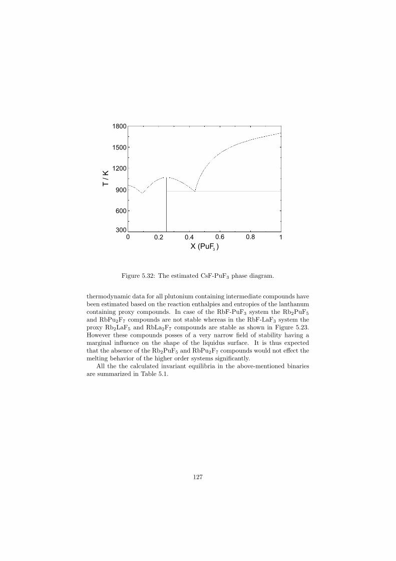
1800

1500

1200

900

600

300

0 0.2 0.4 0.6 0.8 1

X (PuF )3

T / K

Figure 5.32: The estimated CsF-PuF3 phase diagram.

thermodynamic data for all plutonium containing intermediate compounds havebeen estimated based on the reaction enthalpies and entropies of the lanthanumcontaining proxy compounds. In case of the RbF-PuF3 system the Rb2PuF5

and RbPu2F7 compounds are not stable whereas in the RbF-LaF3 system theproxy Rb2LaF5 and RbLa2F7 compounds are stable as shown in Figure 5.23.However these compounds posses of a very narrow field of stability having amarginal influence on the shape of the liquidus surface. It is thus expectedthat the absence of the Rb2PuF5 and RbPu2F7 compounds would not effect themelting behavior of the higher order systems significantly.

All the the calculated invariant equilibria in the above-mentioned binariesare summarized in Table 5.1.

127

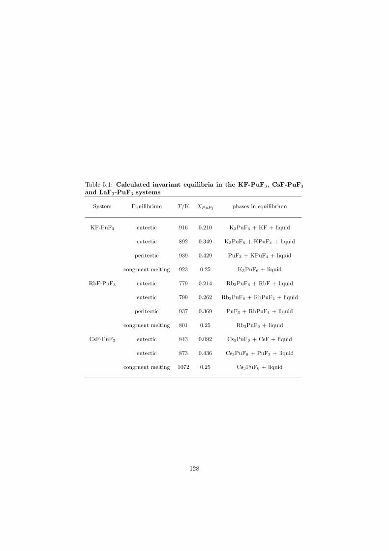
Table 5.1: Calculated invariant equilibria in the KF-PuF3, CsF-PuF3

and LaF3-PuF3 systems

System Equilibrium T/K XPuF3phases in equilibrium

KF-PuF3 eutectic 916 0.210 K3PuF6 + KF + liquid

eutectic 892 0.349 K3PuF6 + KPuF4 + liquid

peritectic 939 0.429 PuF3 + KPuF4 + liquid

congruent melting 923 0.25 K3PuF6 + liquid

RbF-PuF3 eutectic 779 0.214 Rb3PuF6 + RbF + liquid

eutectic 799 0.262 Rb3PuF6 + RbPuF4 + liquid

peritectic 937 0.369 PuF3 + RbPuF4 + liquid

congruent melting 801 0.25 Rb3PuF6 + liquid

CsF-PuF3 eutectic 843 0.092 Cs3PuF6 + CsF + liquid

eutectic 873 0.436 Cs3PuF6 + PuF3 + liquid

congruent melting 1072 0.25 Cs3PuF6 + liquid

128

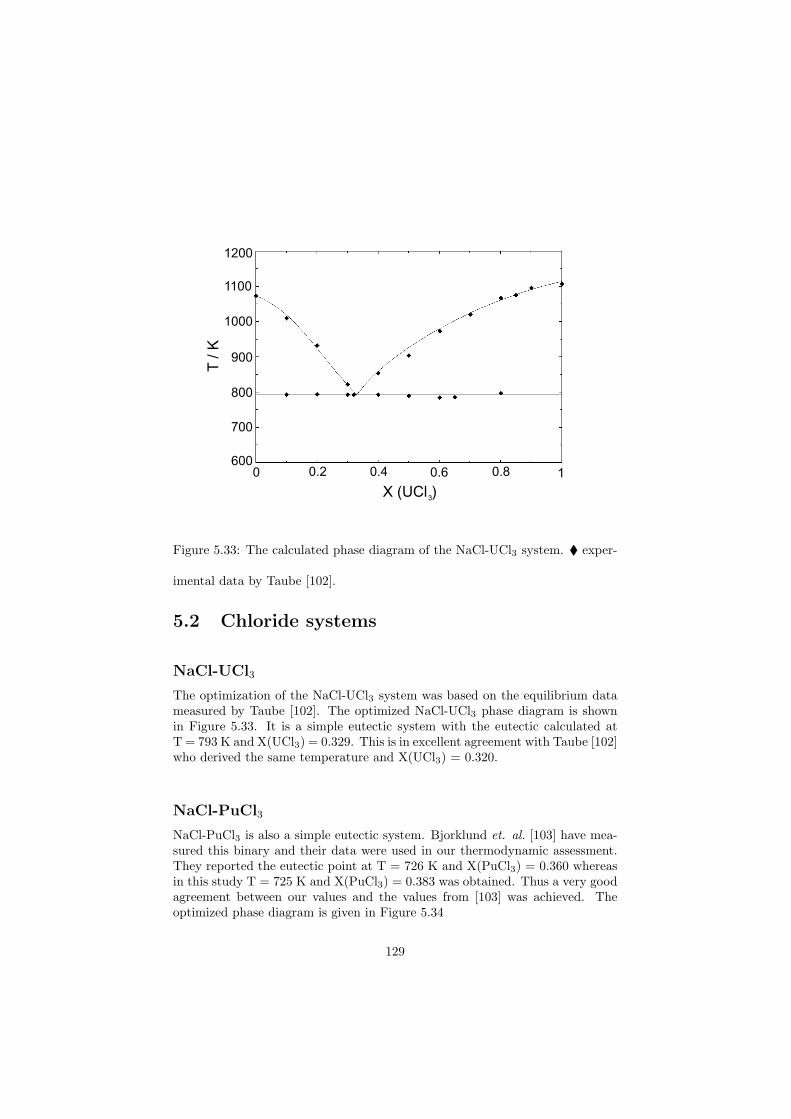
600

800

700

900

1000

1200

1100

0 10.2 0.4 0.80.6

T / K

X (UCl )3

Figure 5.33: The calculated phase diagram of the NaCl-UCl3 system. exper-

imental data by Taube [102].

5.2 Chloride systems

NaCl-UCl3

The optimization of the NaCl-UCl3 system was based on the equilibrium datameasured by Taube [102]. The optimized NaCl-UCl3 phase diagram is shownin Figure 5.33. It is a simple eutectic system with the eutectic calculated atT = 793 K and X(UCl3) = 0.329. This is in excellent agreement with Taube [102]who derived the same temperature and X(UCl3) = 0.320.

NaCl-PuCl3

NaCl-PuCl3 is also a simple eutectic system. Bjorklund et. al. [103] have mea-sured this binary and their data were used in our thermodynamic assessment.They reported the eutectic point at T = 726 K and X(PuCl3) = 0.360 whereasin this study T = 725 K and X(PuCl3) = 0.383 was obtained. Thus a very goodagreement between our values and the values from [103] was achieved. Theoptimized phase diagram is given in Figure 5.34

129

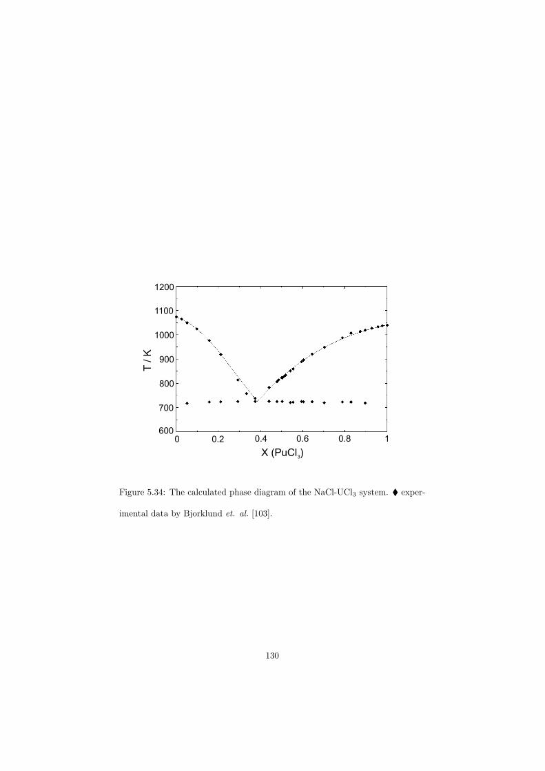
600

900

800

700

1000

1100

1200

0 0.2 0.4 0.6 0.8 1

T / K

X (PuCl )3

Figure 5.34: The calculated phase diagram of the NaCl-UCl3 system. exper-

imental data by Bjorklund et. al. [103].

130

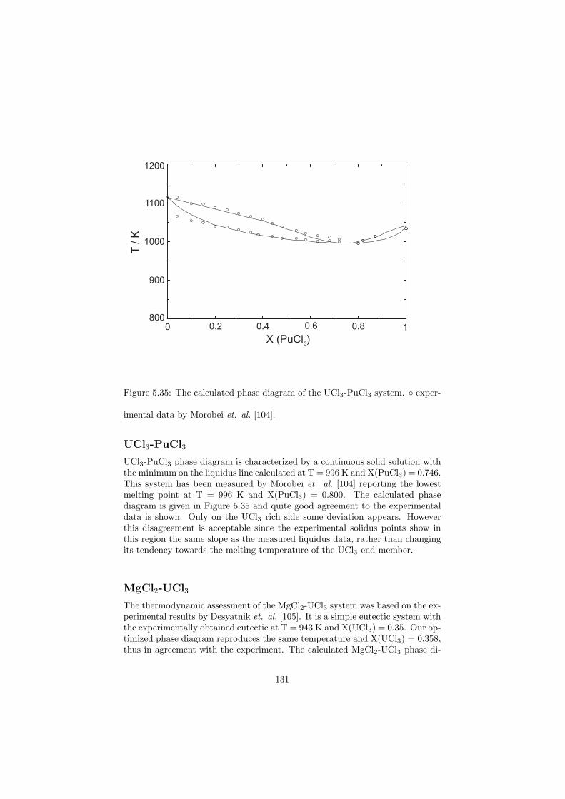
1200

1000

1100

900

800

0 10.2 0.4 0.80.6

X (PuCl )

T / K

3

Figure 5.35: The calculated phase diagram of the UCl3-PuCl3 system. exper-

imental data by Morobei et. al. [104].

UCl3-PuCl3

UCl3-PuCl3 phase diagram is characterized by a continuous solid solution withthe minimum on the liquidus line calculated at T = 996 K and X(PuCl3) = 0.746.This system has been measured by Morobei et. al. [104] reporting the lowestmelting point at T = 996 K and X(PuCl3) = 0.800. The calculated phasediagram is given in Figure 5.35 and quite good agreement to the experimentaldata is shown. Only on the UCl3 rich side some deviation appears. Howeverthis disagreement is acceptable since the experimental solidus points show inthis region the same slope as the measured liquidus data, rather than changingits tendency towards the melting temperature of the UCl3 end-member.

MgCl2-UCl3

The thermodynamic assessment of the MgCl2-UCl3 system was based on the ex-perimental results by Desyatnik et. al. [105]. It is a simple eutectic system withthe experimentally obtained eutectic at T = 943 K and X(UCl3) = 0.35. Our op-timized phase diagram reproduces the same temperature and X(UCl3) = 0.358,thus in agreement with the experiment. The calculated MgCl2-UCl3 phase di-

131

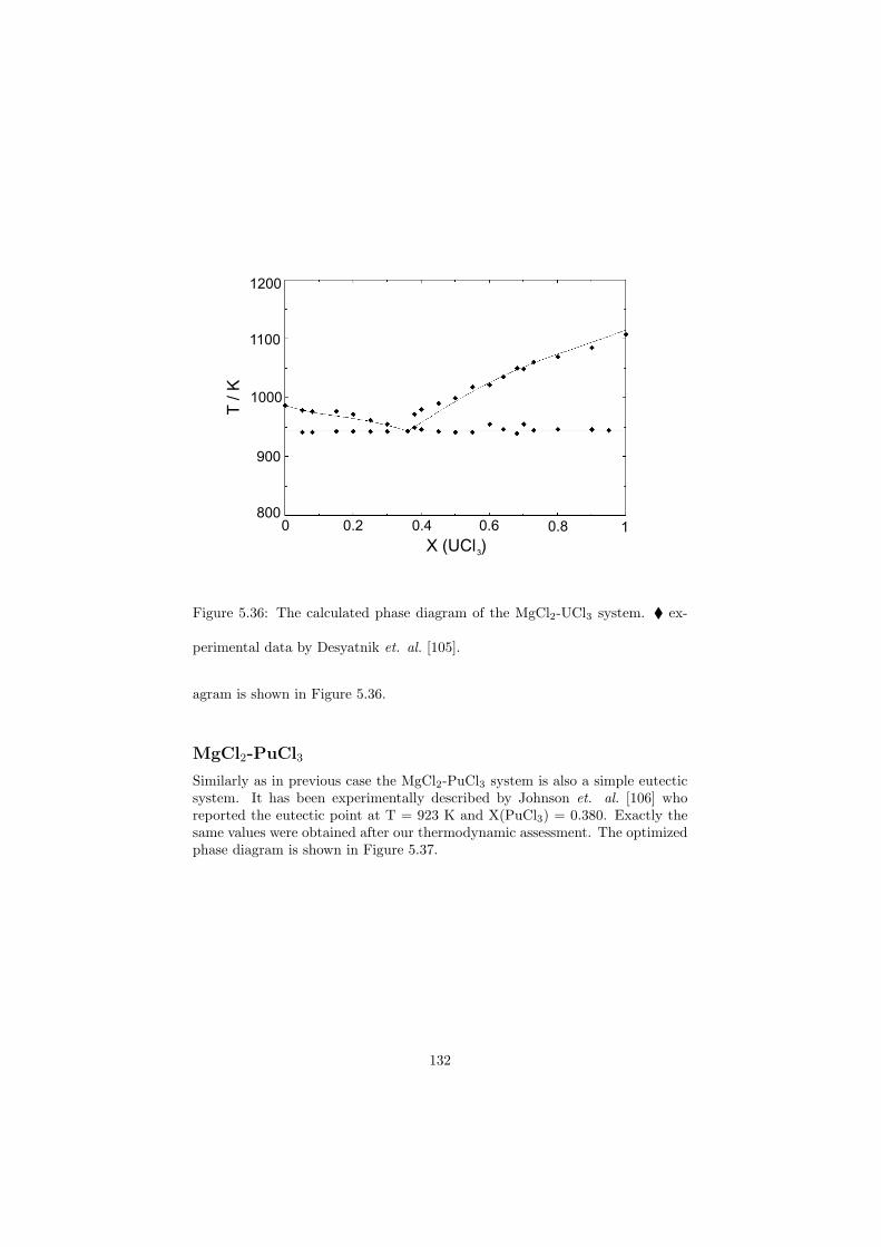
800

1000

900

1100

1200

0 10.2 0.4 0.6 0.8

T / K

X (UCl )3

Figure 5.36: The calculated phase diagram of the MgCl2-UCl3 system. ex-

perimental data by Desyatnik et. al. [105].

agram is shown in Figure 5.36.

MgCl2-PuCl3

Similarly as in previous case the MgCl2-PuCl3 system is also a simple eutecticsystem. It has been experimentally described by Johnson et. al. [106] whoreported the eutectic point at T = 923 K and X(PuCl3) = 0.380. Exactly thesame values were obtained after our thermodynamic assessment. The optimizedphase diagram is shown in Figure 5.37.

132

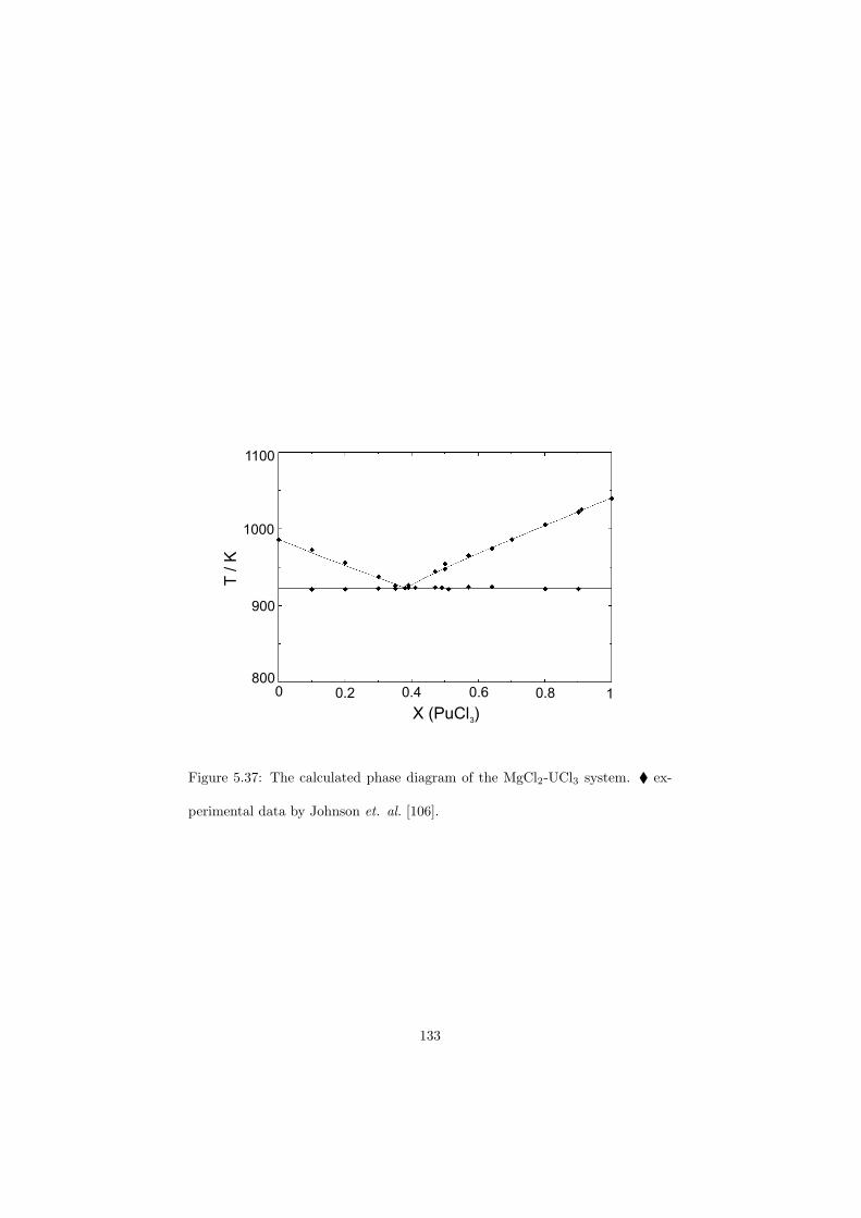
900

800

1100

1000

0 10.2 0.4 0.6 0.8

T / K

X (PuCl )3

Figure 5.37: The calculated phase diagram of the MgCl2-UCl3 system. ex-

perimental data by Johnson et. al. [106].

133

Chapter 6

Ternary systems

In this chapter some of the ternary phase diagrams assessed in this study will beshown. Due to the relatively large amount of the ternary phase diagrams thatcan be generated from our database only the ones that have been experimentallydetermined allowing a comparison between the experiment and the calculationand the ones that are of direct importance for the nuclear applications (fuelmatrixes or heat transfer salts) will be discussed.

The LiF-NaF-KF phase diagram

The LiF-NaF-KF phase diagram is an example of a simple ternary eutecticsystem. As mentioned in [107] the potential of this system in the new generationnuclear reactors is its use as a heat transfer salt to deliver the heat from thehigh temperature reactor core to the hydrogen power plant which would producethe hydrogen gas by water decomposition through the sulfur-iodine cycle. Thisprocess operates at temperatures above 1073 K so a large amount of energy withsmall losses must be delivered from the reactor to the producing plant. Moreoverfor the safety reasons there will be a long distance between these two sites so amedium with low viscosity, high heat capacity and good thermal conductivitywill be necessary. Since a good compromise between these properties is metby the eutectic composition of the LiF-NaF-KF system the thermodynamicdescription of this system is of big importance. Moreover as it is discussed inthe next chapter, this system has been investigated as an alternative matrix forPuF3 dissolution to serve as an actinide burner fuel in the molten salt reactor.

The LiF-NaF-KF phase diagram has been already thermodynamically as-sessed using the classical polynomial model for the description of the liquid

134

and solid solutions [108] and by a modified quasi chemical model in [18]. Inthis study the LiF-NaF-KF phase diagram has been optimized as well and theresult is shown in Figure 6.1 as a projection of liquidus surface. The ternaryeutectic was found at T = 726 K and X(LiF) = 0.453, X(NaF) = 0.132 andX(KF) = 0.415. It is almost identical to the experimentally determined eutecticby Bergman and Dergunov [109] who found T = 727 K and LiF-NaF-KF (46.5-11.5-42.0 mole%). The eutectic temperature T = 727 K has been also confirmedby the DSC measurement performed as part of this work.

The LiF-NaF-RbF phase diagram

Similarly to the previous system, the LiF-NaF-RF system is considered as oneof the alternatives for the fuel matrix for a molten salt reactor. The modelledphase diagram is shown in Figure 6.2 and is characterized by a single ternaryeutectic point. This is in small disagreement to the phase diagram that has beenpublished by Sangster and Pelton in [108] who reported one ternary eutectic andone ternary quasi-peritectic invariant equilibria. However this discrepancy is aconsequence of considering two different versions of the LiF-RbF binary phasediagram. As was already discussed, in our study the thermodynamic assess-ment of this binary was based on the DSC data measured in our laboratory andpublished in [69] which confirmed decomposition of the LiRbF2 compound be-low solidus, whereas the phase diagram from [108] considered this intermediatecompound as melting peritectically and thus a ternary quasi-peritectic appearsin their phase diagram.

The ternary eutectic found on a basis of our calculation is at T = 708 K andX(LiF) = 0.418, X(NaF) = 0.138, X(RbF) = 0.444.

The LiF-NaF-BeF2 phase diagram

The LiF-NaF-BeF2 ternary system has been measured by Moore et al. [110] asreported in [60]. In order to obtain a very good agreement between our cal-culated invariant equilibria and the measured values, the ternary excess Gibbsparameters had to be optimized . The calculated LiF-NaF-BeF2 phase dia-gram is shown in Figure 6.3 as a liquidus projection. It consists of six invari-ant equilibria, five eutectics and one quasi-peritectic, and five saddle points.Their temperatures and compositions are reported in Table 6.1 and a compar-ison to the experimental data [60] is made as well. According to the phasediagram from [60] the system contains four ternary intermediate compoundsLiNaBeF4, LiNa5Be3F12, LiNa2Be2F7 and LiNaBe3F8 which must be consid-ered in the thermodynamic assessment. However, due to the lack of any data theLiNaBe3F8 compound has been neglected while the other three have been opti-mized to reproduce their measured decomposition temperatures [60]. LiNaBeF4

and LiNa5Be3F12 decompose below the solidus at T = 513 K and T = 593 K

135

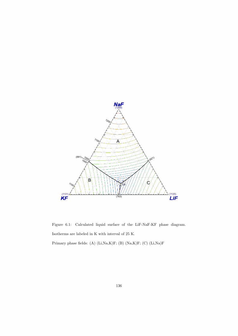
726

(1131) (1120)

(1269)

1100

1000

1000

1100

1200

(921)

(763)

(991)

A

BC

Figure 6.1: Calculated liquid surface of the LiF-NaF-KF phase diagram.

Isotherms are labeled in K with interval of 25 K.

Primary phase fields: (A) (Li,Na,K)F; (B) (Na,K)F; (C) (Li,Na)F

136

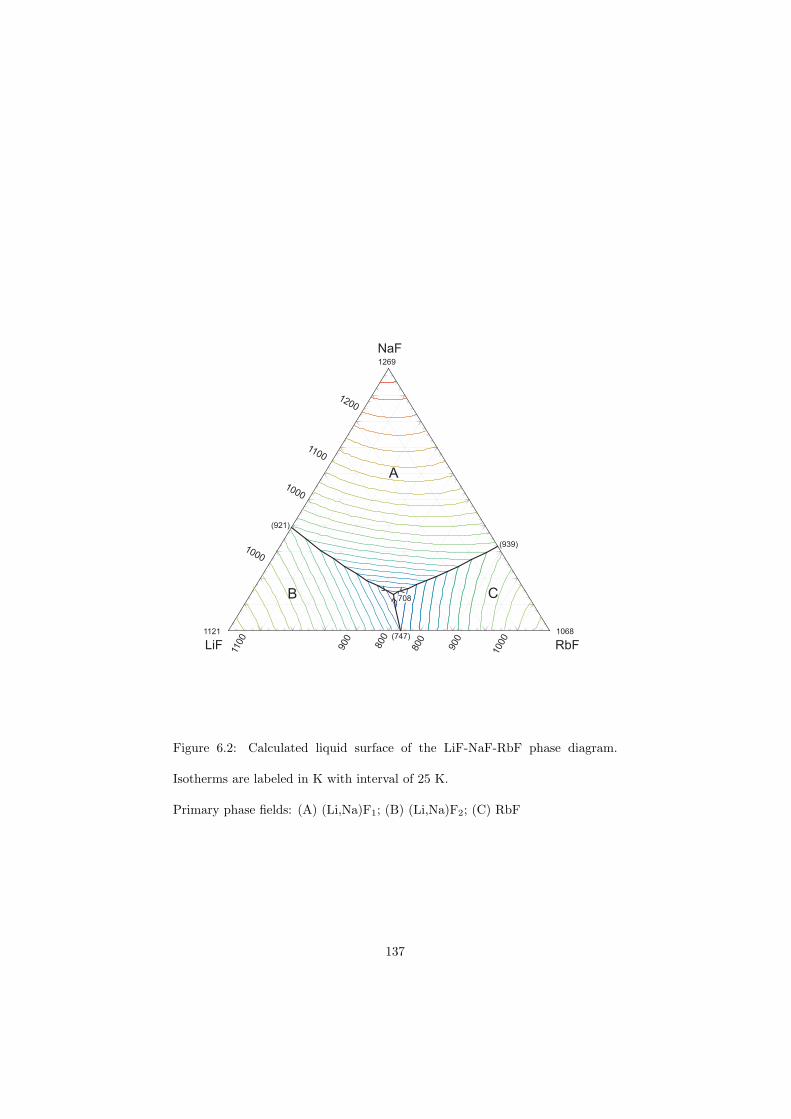
0.1

0.2

0.3

0.4

0.5

0.6

0.7

0.8

0.9

0.10.20.30.40.50.60.70.80.9

0.1

0.2

0.3

0.4

0.5

0.6

0.7

0.8

0.9

NaF

LiF RbFmole fraction /(LiF+NaF+RbF)

NaF

LiF RbFmole fraction /(LiF+NaF+RbF)

NaF

LiF RbFmole fraction /(LiF+NaF+RbF)

NaF

LiF RbFmole fraction /(LiF+NaF+RbF)

NaF

LiF RbFmole fraction /(LiF+NaF+RbF)

NaF

LiF RbFmole fraction /(LiF+NaF+RbF)

NaF

LiF RbFmole fraction /(LiF+NaF+RbF)

NaF

LiF RbFmole fraction /(LiF+NaF+RbF)

NaF

LiF RbFmole fraction /(LiF+NaF+RbF)

NaF

LiF RbFmole fraction /(LiF+NaF+RbF)

NaF

LiF RbFmole fraction /(LiF+NaF+RbF)

NaF

LiF RbFmole fraction /(LiF+NaF+RbF)

NaF

LiF RbFmole fraction /(LiF+NaF+RbF)

NaF

LiF RbFmole fraction /(LiF+NaF+RbF)

NaF

LiF RbFmole fraction /(LiF+NaF+RbF)

NaF

LiF RbFmole fraction /(LiF+NaF+RbF)

NaF

LiF RbFmole fraction /(LiF+NaF+RbF)

NaF

LiF RbFmole fraction /(LiF+NaF+RbF)

NaF

LiF RbFmole fraction /(LiF+NaF+RbF)

NaF

LiF RbFmole fraction /(LiF+NaF+RbF)

NaF

LiF RbFmole fraction /(LiF+NaF+RbF)

NaF

LiF RbFmole fraction /(LiF+NaF+RbF)

NaF

LiF RbFmole fraction /(LiF+NaF+RbF)

NaF

RbFLiF

1269

1121 1068

1200

1100

1000

1000

1100

900

800

800

900

1000(747)

(939)

(921)

708

A

B C

Figure 6.2: Calculated liquid surface of the LiF-NaF-RbF phase diagram.

Isotherms are labeled in K with interval of 25 K.

Primary phase fields: (A) (Li,Na)F1; (B) (Li,Na)F2; (C) RbF

137

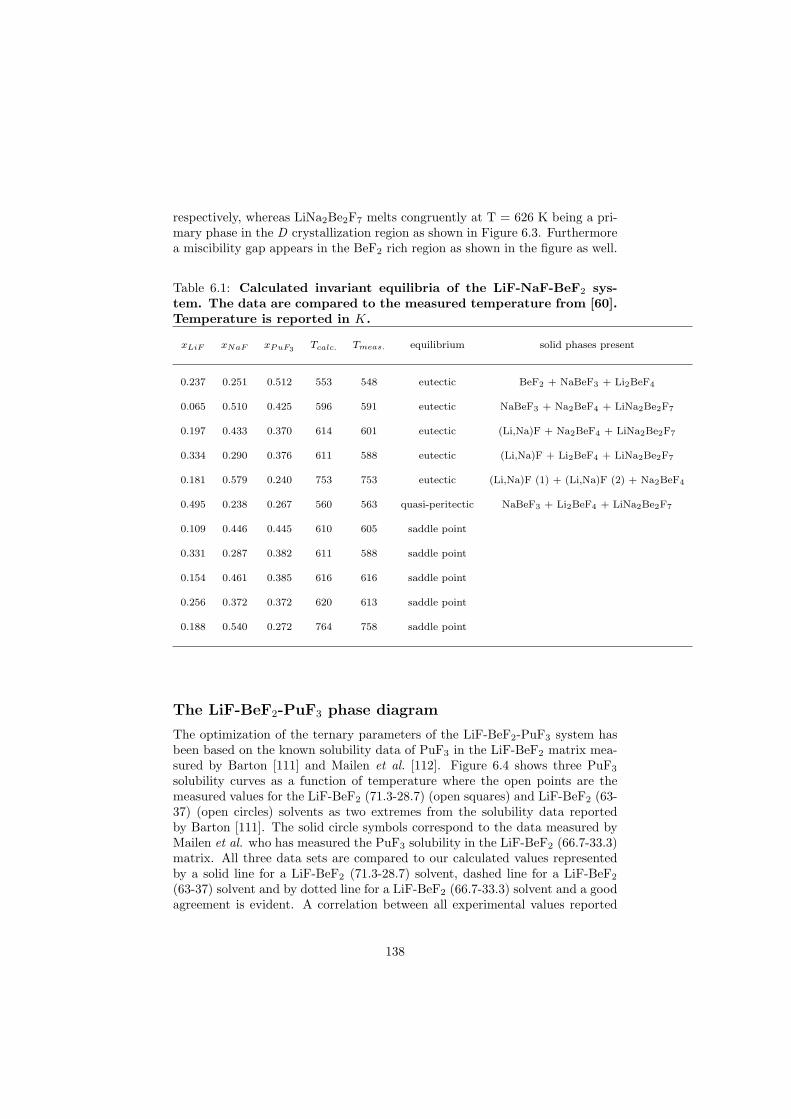
respectively, whereas LiNa2Be2F7 melts congruently at T = 626 K being a pri-mary phase in the D crystallization region as shown in Figure 6.3. Furthermorea miscibility gap appears in the BeF2 rich region as shown in the figure as well.

Table 6.1: Calculated invariant equilibria of the LiF-NaF-BeF2 sys-tem. The data are compared to the measured temperature from [60].Temperature is reported in K.

xLiF xNaF xPuF3Tcalc. Tmeas. equilibrium solid phases present

0.237 0.251 0.512 553 548 eutectic BeF2 + NaBeF3 + Li2BeF4

0.065 0.510 0.425 596 591 eutectic NaBeF3 + Na2BeF4 + LiNa2Be2F7

0.197 0.433 0.370 614 601 eutectic (Li,Na)F + Na2BeF4 + LiNa2Be2F7

0.334 0.290 0.376 611 588 eutectic (Li,Na)F + Li2BeF4 + LiNa2Be2F7

0.181 0.579 0.240 753 753 eutectic (Li,Na)F (1) + (Li,Na)F (2) + Na2BeF4

0.495 0.238 0.267 560 563 quasi-peritectic NaBeF3 + Li2BeF4 + LiNa2Be2F7

0.109 0.446 0.445 610 605 saddle point

0.331 0.287 0.382 611 588 saddle point

0.154 0.461 0.385 616 616 saddle point

0.256 0.372 0.372 620 613 saddle point

0.188 0.540 0.272 764 758 saddle point

The LiF-BeF2-PuF3 phase diagram

The optimization of the ternary parameters of the LiF-BeF2-PuF3 system hasbeen based on the known solubility data of PuF3 in the LiF-BeF2 matrix mea-sured by Barton [111] and Mailen et al. [112]. Figure 6.4 shows three PuF3

solubility curves as a function of temperature where the open points are themeasured values for the LiF-BeF2 (71.3-28.7) (open squares) and LiF-BeF2 (63-37) (open circles) solvents as two extremes from the solubility data reportedby Barton [111]. The solid circle symbols correspond to the data measured byMailen et al. who has measured the PuF3 solubility in the LiF-BeF2 (66.7-33.3)matrix. All three data sets are compared to our calculated values representedby a solid line for a LiF-BeF2 (71.3-28.7) solvent, dashed line for a LiF-BeF2

(63-37) solvent and by dotted line for a LiF-BeF2 (66.7-33.3) solvent and a goodagreement is evident. A correlation between all experimental values reported

138

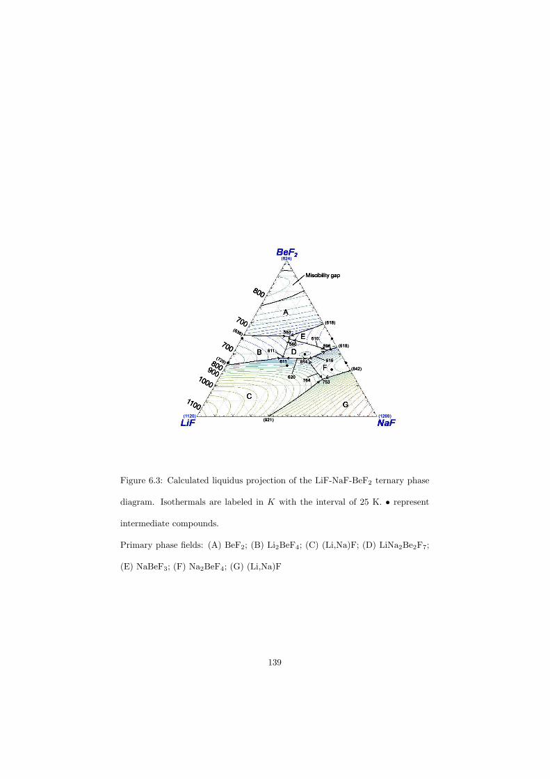
Figure 6.3: Calculated liquidus projection of the LiF-NaF-BeF2 ternary phase

diagram. Isothermals are labeled in K with the interval of 25 K. • represent

intermediate compounds.

Primary phase fields: (A) BeF2; (B) Li2BeF4; (C) (Li,Na)F; (D) LiNa2Be2F7;

(E) NaBeF3; (F) Na2BeF4; (G) (Li,Na)F

139

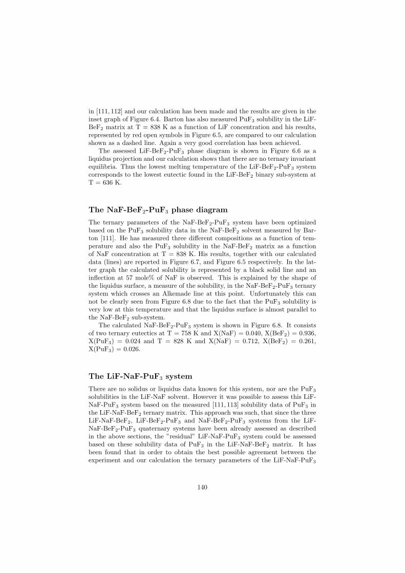
in [111, 112] and our calculation has been made and the results are given in theinset graph of Figure 6.4. Barton has also measured PuF3 solubility in the LiF-BeF2 matrix at T = 838 K as a function of LiF concentration and his results,represented by red open symbols in Figure 6.5, are compared to our calculationshown as a dashed line. Again a very good correlation has been achieved.

The assessed LiF-BeF2-PuF3 phase diagram is shown in Figure 6.6 as aliquidus projection and our calculation shows that there are no ternary invariantequilibria. Thus the lowest melting temperature of the LiF-BeF2-PuF3 systemcorresponds to the lowest eutectic found in the LiF-BeF2 binary sub-system atT = 636 K.

The NaF-BeF2-PuF3 phase diagram

The ternary parameters of the NaF-BeF2-PuF3 system have been optimizedbased on the PuF3 solubility data in the NaF-BeF2 solvent measured by Bar-ton [111]. He has measured three different compositions as a function of tem-perature and also the PuF3 solubility in the NaF-BeF2 matrix as a functionof NaF concentration at T = 838 K. His results, together with our calculateddata (lines) are reported in Figure 6.7, and Figure 6.5 respectively. In the lat-ter graph the calculated solubility is represented by a black solid line and aninflection at 57 mole% of NaF is observed. This is explained by the shape ofthe liquidus surface, a measure of the solubility, in the NaF-BeF2-PuF3 ternarysystem which crosses an Alkemade line at this point. Unfortunately this cannot be clearly seen from Figure 6.8 due to the fact that the PuF3 solubility isvery low at this temperature and that the liquidus surface is almost parallel tothe NaF-BeF2 sub-system.

The calculated NaF-BeF2-PuF3 system is shown in Figure 6.8. It consistsof two ternary eutectics at T = 758 K and X(NaF) = 0.040, X(BeF2) = 0.936,X(PuF3) = 0.024 and T = 828 K and X(NaF) = 0.712, X(BeF2) = 0.261,X(PuF3) = 0.026.

The LiF-NaF-PuF3 system

There are no solidus or liquidus data known for this system, nor are the PuF3

solubilities in the LiF-NaF solvent. However it was possible to assess this LiF-NaF-PuF3 system based on the measured [111, 113] solubility data of PuF3 inthe LiF-NaF-BeF2 ternary matrix. This approach was such, that since the threeLiF-NaF-BeF2, LiF-BeF2-PuF3 and NaF-BeF2-PuF3 systems from the LiF-NaF-BeF2-PuF3 quaternary systems have been already assessed as describedin the above sections, the ”residual” LiF-NaF-PuF3 system could be assessedbased on these solubility data of PuF3 in the LiF-NaF-BeF2 matrix. It hasbeen found that in order to obtain the best possible agreement between theexperiment and our calculation the ternary parameters of the LiF-NaF-PuF3

140

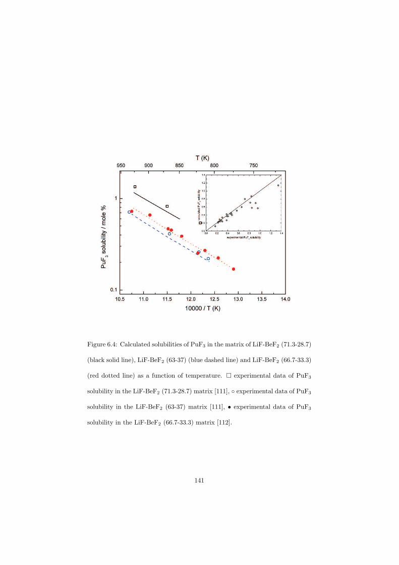
Figure 6.4: Calculated solubilities of PuF3 in the matrix of LiF-BeF2 (71.3-28.7)

(black solid line), LiF-BeF2 (63-37) (blue dashed line) and LiF-BeF2 (66.7-33.3)

(red dotted line) as a function of temperature. experimental data of PuF3

solubility in the LiF-BeF2 (71.3-28.7) matrix [111], experimental data of PuF3

solubility in the LiF-BeF2 (63-37) matrix [111], • experimental data of PuF3

solubility in the LiF-BeF2 (66.7-33.3) matrix [112].

141

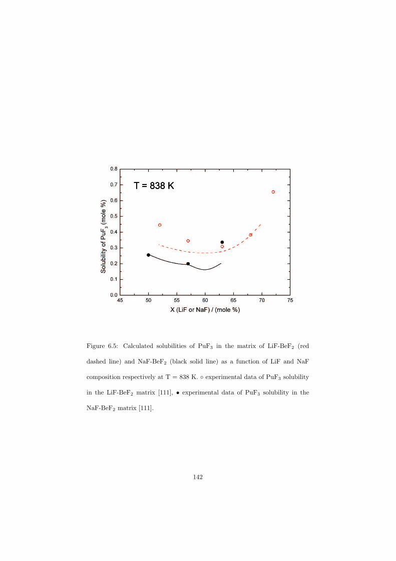
Figure 6.5: Calculated solubilities of PuF3 in the matrix of LiF-BeF2 (red

dashed line) and NaF-BeF2 (black solid line) as a function of LiF and NaF

composition respectively at T = 838 K. experimental data of PuF3 solubility

in the LiF-BeF2 matrix [111], • experimental data of PuF3 solubility in the

NaF-BeF2 matrix [111].

142

Figure 6.6: Calculated liquidus projection of the LiF-BeF2-PuF3 ternary phase

diagram. Isothermals are labelled in K with the interval of 25 K.

Primary phase fields: (A) PuF3; (B) LiF; (C) BeF2

143

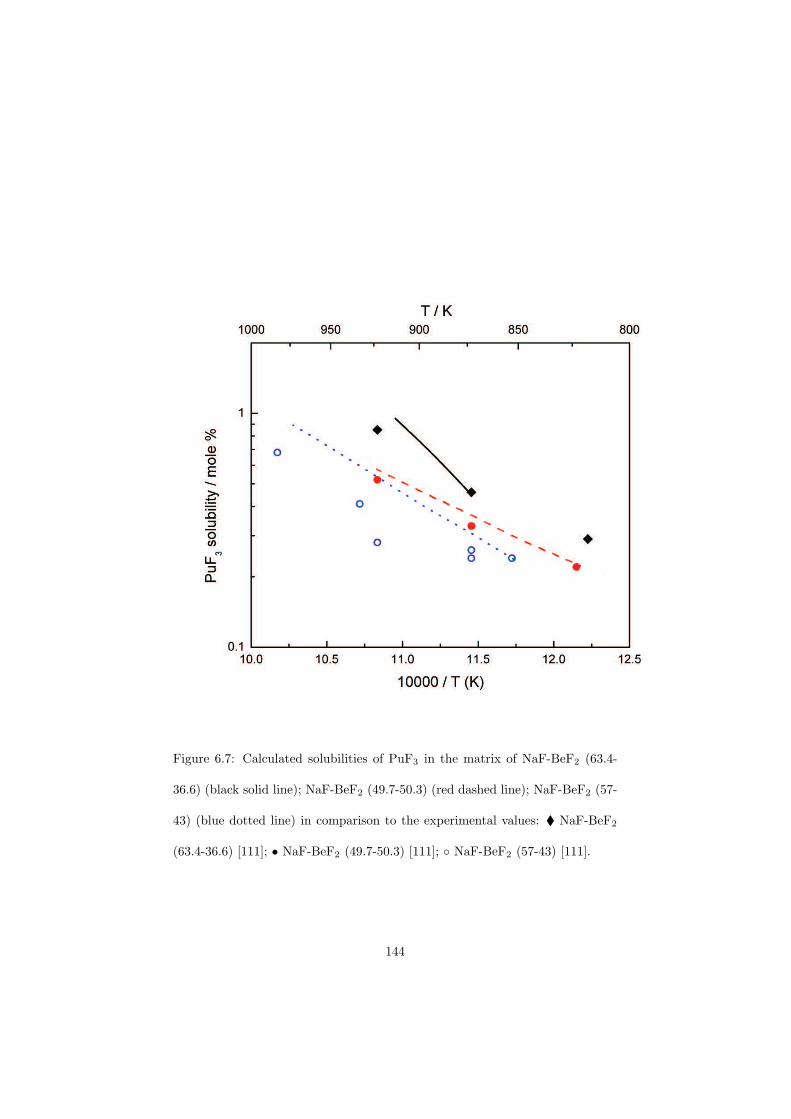
Figure 6.7: Calculated solubilities of PuF3 in the matrix of NaF-BeF2 (63.4-

36.6) (black solid line); NaF-BeF2 (49.7-50.3) (red dashed line); NaF-BeF2 (57-

43) (blue dotted line) in comparison to the experimental values: NaF-BeF2

(63.4-36.6) [111]; • NaF-BeF2 (49.7-50.3) [111]; NaF-BeF2 (57-43) [111].

144

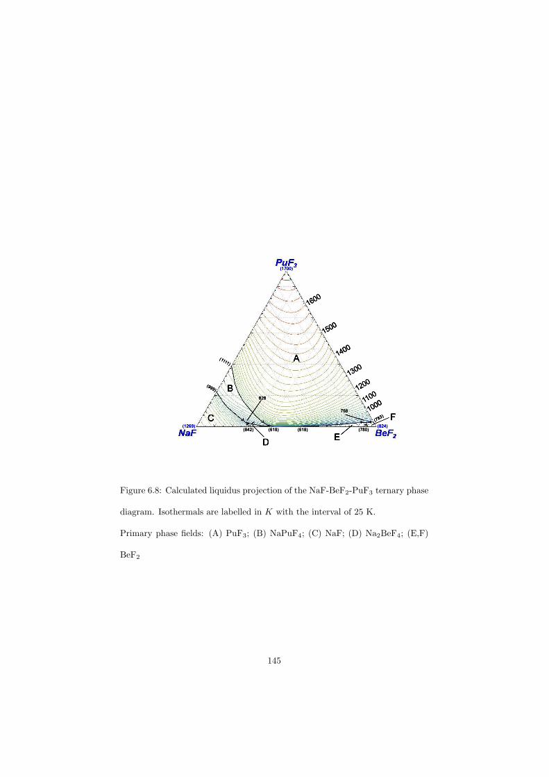
Figure 6.8: Calculated liquidus projection of the NaF-BeF2-PuF3 ternary phase

diagram. Isothermals are labelled in K with the interval of 25 K.

Primary phase fields: (A) PuF3; (B) NaPuF4; (C) NaF; (D) Na2BeF4; (E,F)

BeF2

145

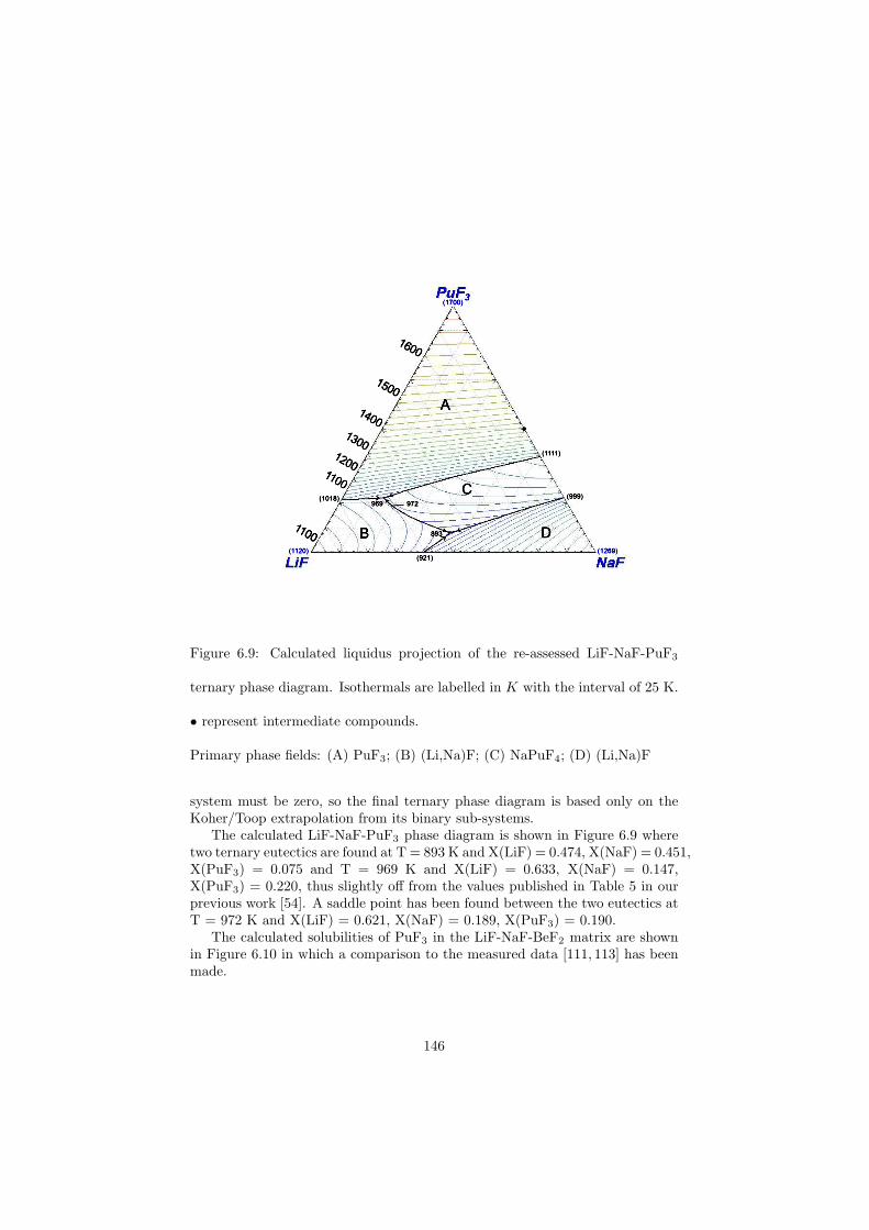
Figure 6.9: Calculated liquidus projection of the re-assessed LiF-NaF-PuF3

ternary phase diagram. Isothermals are labelled in K with the interval of 25 K.

• represent intermediate compounds.

Primary phase fields: (A) PuF3; (B) (Li,Na)F; (C) NaPuF4; (D) (Li,Na)F

system must be zero, so the final ternary phase diagram is based only on theKoher/Toop extrapolation from its binary sub-systems.

The calculated LiF-NaF-PuF3 phase diagram is shown in Figure 6.9 wheretwo ternary eutectics are found at T = 893 K and X(LiF) = 0.474, X(NaF) = 0.451,X(PuF3) = 0.075 and T = 969 K and X(LiF) = 0.633, X(NaF) = 0.147,X(PuF3) = 0.220, thus slightly off from the values published in Table 5 in ourprevious work [54]. A saddle point has been found between the two eutectics atT = 972 K and X(LiF) = 0.621, X(NaF) = 0.189, X(PuF3) = 0.190.

The calculated solubilities of PuF3 in the LiF-NaF-BeF2 matrix are shownin Figure 6.10 in which a comparison to the measured data [111, 113] has beenmade.

146

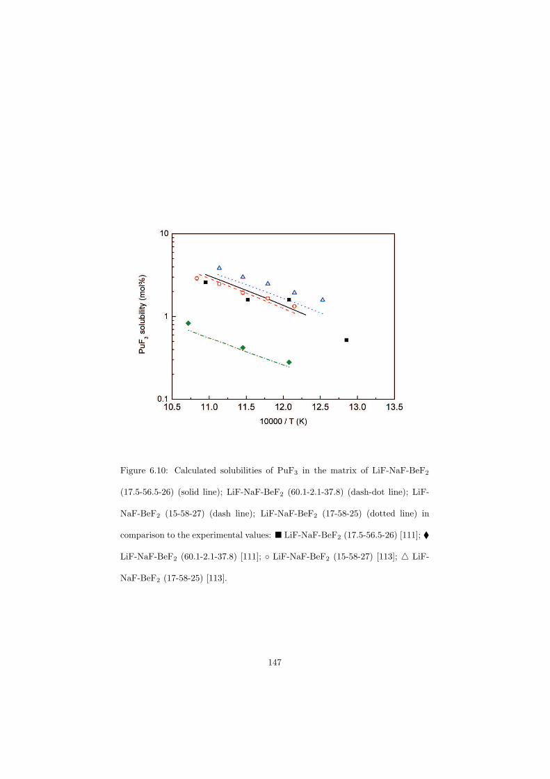
Figure 6.10: Calculated solubilities of PuF3 in the matrix of LiF-NaF-BeF2

(17.5-56.5-26) (solid line); LiF-NaF-BeF2 (60.1-2.1-37.8) (dash-dot line); LiF-

NaF-BeF2 (15-58-27) (dash line); LiF-NaF-BeF2 (17-58-25) (dotted line) in

comparison to the experimental values: LiF-NaF-BeF2 (17.5-56.5-26) [111];

LiF-NaF-BeF2 (60.1-2.1-37.8) [111]; LiF-NaF-BeF2 (15-58-27) [113]; LiF-

NaF-BeF2 (17-58-25) [113].

147

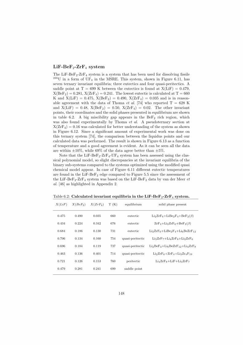
LiF-BeF2-ZrF4 system

The LiF-BeF2-ZrF4 system is a system that has been used for dissolving fissile235U in a form of UF4 in the MSRE. This system, shown in Figure 6.11, hasseven ternary invariant equilibria; three eutectics and four quasi-peritectics. Asaddle point at T = 699 K between the eutectics is found at X(LiF) = 0.479,X(BeF2) = 0.281, X(ZrF4) = 0.241. The lowest eutectic is calculated at T = 660K and X(LiF) = 0.475, X(BeF2) = 0.490, X(ZrF4) = 0.035 and is in reason-able agreement with the data of Thoma et al. [74] who reported T = 628 Kand X(LiF) = 0.48, X(BeF2) = 0.50, X(ZrF4) = 0.02. The other invariantpoints, their coordinates and the solid phases presented in equilibrium are shownin table 6.2. A big miscibility gap appears in the BeF2 rich region, whichwas also found experimentally by Thoma et al. A pseudoternary section atX(ZrF4) = 0.16 was calculated for better understanding of the system as shownin Figure 6.12. Since a significant amount of experimental work was done onthis ternary system [74], the comparison between the liquidus points and ourcalculated data was performed. The result is shown in Figure 6.13 as a functionof temperature and a good agreement is evident. As it can be seen all the dataare within ±10%, while 69% of the data agree better than ±5%.

Note that the LiF-BeF2-ZrF4-UF4 system has been assessed using the clas-sical polynomial model, so slight discrepancies at the invariant equilibria of thebinary sub-systems compared to the systems optimized using the modified quasichemical model appear. In case of Figure 6.11 different eutectic temperaturesare found in the LiF-BeF2 edge compared to Figure 5.5 since the assessment ofthe LiF-BeF2-ZrF4 system was based on the LiF-BeF2 data by van der Meer etal. [46] as highlighted in Appendix 2.

Table 6.2: Calculated invariant equilibria in the LiF-BeF2-ZrF4 system.

X(LiF ) X(BeF2) X(ZrF4) T (K) equilibrium solid phase present

0.475 0.490 0.035 660 eutectic Li2ZrF6+LiBe2F4+BeF2(β)

0.434 0.224 0.342 676 eutectic ZrF4+Li2ZrF6+BeF2(β)

0.684 0.186 0.130 731 eutectic Li2ZrF6+LiBe2F4+Li6BeZrF12

0.706 0.134 0.160 754 quasi-peritectic Li3ZrF7+Li4ZrF8+Li2ZrF6

0.696 0.184 0.119 737 quasi-peritectic Li2BeF4+Li6BeZrF12+Li4ZrF8

0.463 0.136 0.401 714 quasi-peritectic Li2ZrF6+ZrF4+Li3Zr4F19

0.721 0.126 0.153 760 peritectic Li4ZrF8+LiF+Li3ZrF7

0.479 0.281 0.241 699 saddle point

148

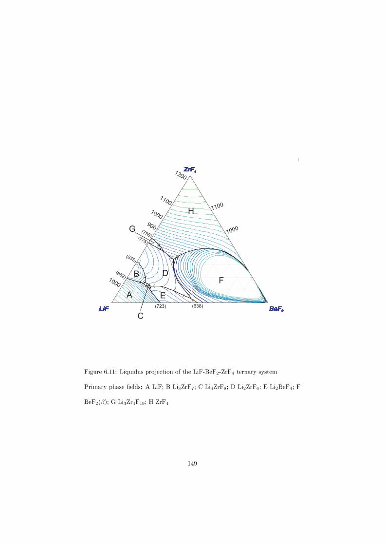
0.1

0.2

0.3

0.4

0.5

0.6

0.7

0.8

0.9

0.10.20.30.40.50.60.70.80.9

0.1

0.2

0.3

0.4

0.5

0.6

0.7

0.8

0.9

ZrF4

LiF BeF2

mole fraction

ZrF4

LiF BeF2

mole fraction

ZrF4

LiF BeF2

mole fraction

ZrF4

LiF BeF2

mole fraction

ZrF4

LiF BeF2

mole fraction

ZrF4

LiF BeF2

mole fraction

ZrF4

LiF BeF2

mole fraction

ZrF4

LiF BeF2

mole fraction

ZrF4

LiF BeF2

mole fraction

ZrF4

LiF BeF2

mole fraction

ZrF4

LiF BeF2

mole fraction

ZrF4

LiF BeF2

mole fraction

ZrF4

LiF BeF2

mole fraction

ZrF4

LiF BeF2

mole fraction

ZrF4

LiF BeF2

mole fraction

ZrF4

LiF BeF2

mole fraction

ZrF4

LiF BeF2

mole fraction

ZrF4

LiF BeF2

mole fraction

ZrF4

LiF BeF2

mole fraction

ZrF4

LiF BeF2

mole fraction

ZrF4

LiF BeF2

mole fraction

ZrF4

LiF BeF2

mole fraction

ZrF4

LiF BeF2

mole fraction

ZrF4

LiF BeF2

mole fraction

ZrF4

LiF BeF2

mole fraction

ZrF4

LiF BeF2

mole fraction

ZrF4

LiF BeF2

mole fraction

ZrF4

LiF BeF2

mole fraction

ZrF4

LiF BeF2

mole fraction

ZrF4

LiF BeF2

mole fraction

ZrF4

LiF BeF2

mole fraction

ZrF4

LiF BeF2

mole fraction

ZrF4

LiF BeF2

mole fraction

ZrF4

LiF BeF2

mole fraction

ZrF4

LiF BeF2

mole fraction

ZrF4

LiF BeF2

mole fraction

ZrF4

LiF BeF2

mole fraction

ZrF4

LiF BeF2

mole fraction

ZrF4

LiF BeF2

mole fraction

ZrF4

LiF BeF2

mole fraction

ZrF4

LiF BeF2

mole fraction

ZrF4

LiF BeF2

mole fraction

ZrF4

LiF BeF2

mole fraction

ZrF4

LiF BeF2

mole fraction

ZrF4

LiF BeF2

mole fraction

ZrF4 - LiF - BeF2

Polythermal projection 675 - 180011/09/2006

C:\FactSage\Figures\LiF-BeF2-ZrF4\Liquid surface 670-1800 by 25.wmf

1200

1100

1000

900

1000

1100

1000

A

B

C

E

FD

G

H

(723) (638)

(882)

(855)

(775)

(798)

Figure 6.11: Liquidus projection of the LiF-BeF2-ZrF4 ternary system

Primary phase fields: A LiF; B Li3ZrF7; C Li4ZrF8; D Li2ZrF6; E Li2BeF4; F

BeF2(β); G Li3Zr4F19; H ZrF4

149

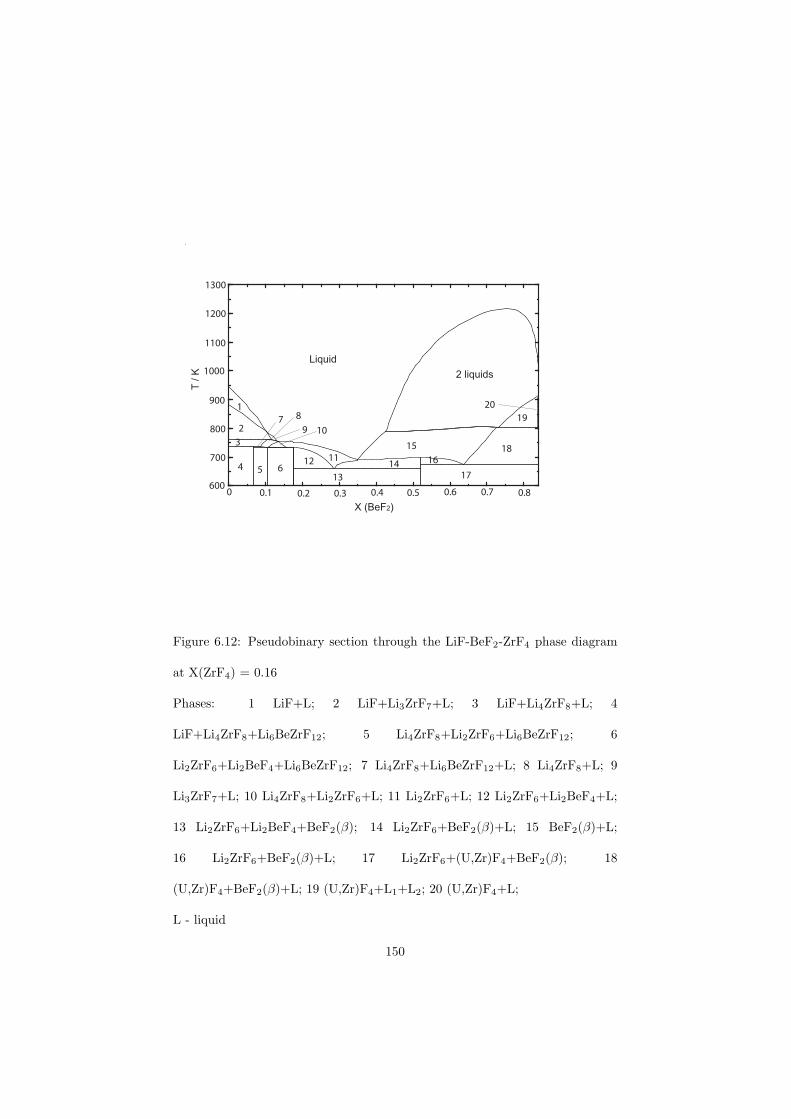
mole BeF2/(ZrF4+LiF+BeF2+UF4)

T(K

)

0 .1 .2 .3 .4 .5 .6 .7 .8

600

700

800

900

1000

1100

1200

1300

Liquid

2 liquids

X (BeF2)

T / K

Figure 6.12: Pseudobinary section through the LiF-BeF2-ZrF4 phase diagram

at X(ZrF4) = 0.16

Phases: 1 LiF+L; 2 LiF+Li3ZrF7+L; 3 LiF+Li4ZrF8+L; 4

LiF+Li4ZrF8+Li6BeZrF12; 5 Li4ZrF8+Li2ZrF6+Li6BeZrF12; 6

Li2ZrF6+Li2BeF4+Li6BeZrF12; 7 Li4ZrF8+Li6BeZrF12+L; 8 Li4ZrF8+L; 9

Li3ZrF7+L; 10 Li4ZrF8+Li2ZrF6+L; 11 Li2ZrF6+L; 12 Li2ZrF6+Li2BeF4+L;

13 Li2ZrF6+Li2BeF4+BeF2(β); 14 Li2ZrF6+BeF2(β)+L; 15 BeF2(β)+L;

16 Li2ZrF6+BeF2(β)+L; 17 Li2ZrF6+(U,Zr)F4+BeF2(β); 18

(U,Zr)F4+BeF2(β)+L; 19 (U,Zr)F4+L1+L2; 20 (U,Zr)F4+L;

L - liquid

150

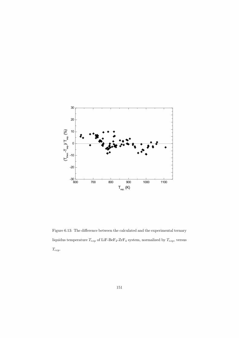
600 700 800 900 1000 1100-30

-20

-10

0

10

20

30

(Tth

eor.-T

exp

.)/ T

exp

. (%

)

Texp.

(K)

Figure 6.13: The difference between the calculated and the experimental ternary

liquidus temperature Texp of LiF-BeF2-ZrF4 system, normalized by Texp, versus

Texp.

151

Chapter 7

Nuclear Fuel Compositions

In this chapter the strength of the thermodynamic modelling as a tool to find oroptimize the fuel choice for a molten salt reactor is demonstrated. It is shownhow the properties like melting temperature, vapour pressure or the solubilityof the actinides in the fuel matrix can be derived based on the thermodynamicassessment. In general, this chapter is divided into four main sections, each onededicated to a unique system that is considered as a possible candidate for amolten salt fuel.

The first system which has been thermodynamically described in this studyis the LiF-BeF2-ZrF4-UF4 system, a system that has already been used as afuel for the MSRE which was a testing reactor in ORNL operating in a thermalneutron spectrum.

LiF-NaF-BeF2-PuF3 is the next system discussed in this work. As reportedin [7] the fuel of the MOSART concept is based on this system. Due to the highviscosity of BeF2 and also due to its toxicity, it was part of this study to try tofind a replacement for BeF2 on a basis of our thermodynamic model. Moreoverit has been demonstrated in previous studies that better AnF3 (An = actinide)solubility is achieved when BeF2 is avoided. Therefore the LiF-NaF-KF-RbF-PuF3 system has been thermodynamically assessed, where the KF and RbFcompounds are believed to be good candidates for this substitution. MoreoverCsF has been added to this system to simulate the fuel behaviour containingcertain concentrations of this fission product. It has been mentioned in the”Nuclear” chapter that a molten salt reactor is designed in such way that anonline clean-up of the fuel is performed. However it will be very difficult toelectrochemically separate CsF from the fuel salt since the standard potentialsof CsF and other alkali halides are very close, especially when RbF is present.

The NaCl-MgCl2-UCl3-PuCl3 system is the last system which has been

152

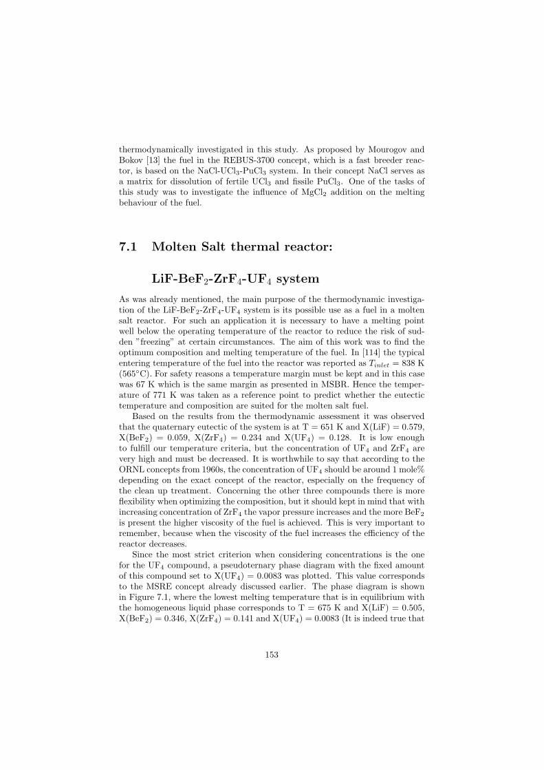
thermodynamically investigated in this study. As proposed by Mourogov andBokov [13] the fuel in the REBUS-3700 concept, which is a fast breeder reac-tor, is based on the NaCl-UCl3-PuCl3 system. In their concept NaCl serves asa matrix for dissolution of fertile UCl3 and fissile PuCl3. One of the tasks ofthis study was to investigate the influence of MgCl2 addition on the meltingbehaviour of the fuel.

7.1 Molten Salt thermal reactor:

LiF-BeF2-ZrF4-UF4 system

As was already mentioned, the main purpose of the thermodynamic investiga-tion of the LiF-BeF2-ZrF4-UF4 system is its possible use as a fuel in a moltensalt reactor. For such an application it is necessary to have a melting pointwell below the operating temperature of the reactor to reduce the risk of sud-den ”freezing” at certain circumstances. The aim of this work was to find theoptimum composition and melting temperature of the fuel. In [114] the typicalentering temperature of the fuel into the reactor was reported as Tinlet = 838 K(565C). For safety reasons a temperature margin must be kept and in this casewas 67 K which is the same margin as presented in MSBR. Hence the temper-ature of 771 K was taken as a reference point to predict whether the eutectictemperature and composition are suited for the molten salt fuel.

Based on the results from the thermodynamic assessment it was observedthat the quaternary eutectic of the system is at T = 651 K and X(LiF) = 0.579,X(BeF2) = 0.059, X(ZrF4) = 0.234 and X(UF4) = 0.128. It is low enoughto fulfill our temperature criteria, but the concentration of UF4 and ZrF4 arevery high and must be decreased. It is worthwhile to say that according to theORNL concepts from 1960s, the concentration of UF4 should be around 1 mole%depending on the exact concept of the reactor, especially on the frequency ofthe clean up treatment. Concerning the other three compounds there is moreflexibility when optimizing the composition, but it should kept in mind that withincreasing concentration of ZrF4 the vapor pressure increases and the more BeF2

is present the higher viscosity of the fuel is achieved. This is very important toremember, because when the viscosity of the fuel increases the efficiency of thereactor decreases.

Since the most strict criterion when considering concentrations is the onefor the UF4 compound, a pseudoternary phase diagram with the fixed amountof this compound set to X(UF4) = 0.0083 was plotted. This value correspondsto the MSRE concept already discussed earlier. The phase diagram is shownin Figure 7.1, where the lowest melting temperature that is in equilibrium withthe homogeneous liquid phase corresponds to T = 675 K and X(LiF) = 0.505,X(BeF2) = 0.346, X(ZrF4) = 0.141 and X(UF4) = 0.0083 (It is indeed true that

153

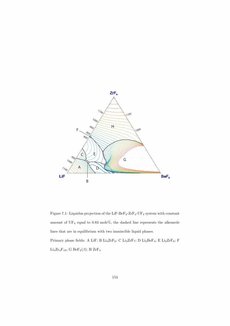
0.1

0.2

0.3

0.4

0.5

0.6

0.7

0.8

0.9

0.10.20.30.40.50.60.70.80.9

0.1

0.2

0.3

0.4

0.5

0.6

0.7

0.8

0.9

ZrF4

LiF BeF2mole fraction /(LiF+ZrF4+BeF2)

ZrF4

LiF BeF2mole fraction /(LiF+ZrF4+BeF2)

ZrF4

LiF BeF2mole fraction /(LiF+ZrF4+BeF2)

ZrF4

LiF BeF2mole fraction /(LiF+ZrF4+BeF2)

ZrF4

LiF BeF2mole fraction /(LiF+ZrF4+BeF2)

ZrF4

LiF BeF2mole fraction /(LiF+ZrF4+BeF2)

ZrF4

LiF BeF2mole fraction /(LiF+ZrF4+BeF2)

ZrF4

LiF BeF2mole fraction /(LiF+ZrF4+BeF2)

ZrF4

LiF BeF2mole fraction /(LiF+ZrF4+BeF2)

ZrF4

LiF BeF2mole fraction /(LiF+ZrF4+BeF2)

ZrF4

LiF BeF2mole fraction /(LiF+ZrF4+BeF2)

ZrF4

LiF BeF2mole fraction /(LiF+ZrF4+BeF2)

ZrF4

LiF BeF2mole fraction /(LiF+ZrF4+BeF2)

ZrF4

LiF BeF2mole fraction /(LiF+ZrF4+BeF2)

ZrF4

LiF BeF2mole fraction /(LiF+ZrF4+BeF2)

ZrF4

LiF BeF2mole fraction /(LiF+ZrF4+BeF2)

ZrF4

LiF BeF2mole fraction /(LiF+ZrF4+BeF2)

ZrF4

LiF BeF2mole fraction /(LiF+ZrF4+BeF2)

ZrF4

LiF BeF2mole fraction /(LiF+ZrF4+BeF2)

ZrF4

LiF BeF2mole fraction /(LiF+ZrF4+BeF2)

ZrF4

LiF BeF2mole fraction /(LiF+ZrF4+BeF2)

ZrF4

LiF BeF2mole fraction /(LiF+ZrF4+BeF2)

1100

1000

900

800

800

900

1000

1100

1100

1000

A

B

C

D

E

F

G

H

Figure 7.1: Liquidus projection of the LiF-BeF2-ZrF4-UF4 system with constant

amount of UF4 equal to 0.83 mole%, the dashed line represents the alkemede

lines that are in equilibrium with two immiscible liquid phases.

Primary phase fields: A LiF; B Li4ZrF8; C Li3ZrF7; D Li2BeF4; E Li2ZrF6; F

Li3Zr4F19; G BeF2(β); H ZrF4

154

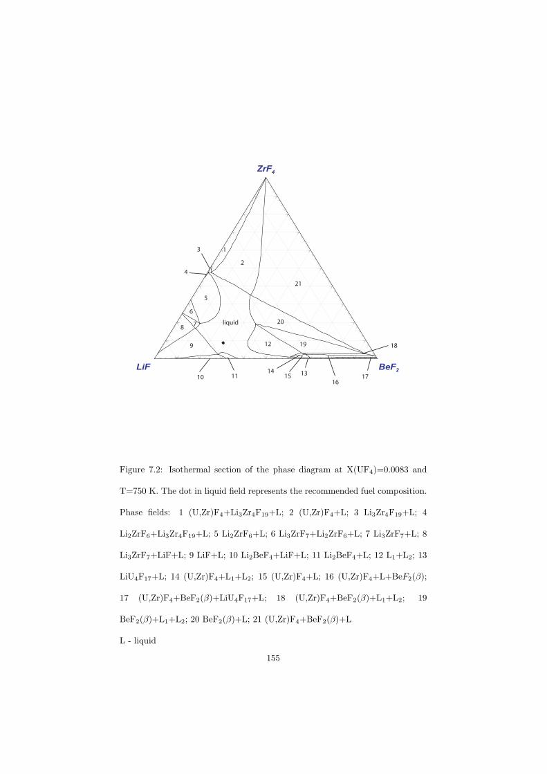
0.1

0.2

0.3

0.4

0.5

0.6

0.7

0.8

0.9

0.10.20.30.40.50.60.70.80.9

0.1

0.2

0.3

0.4

0.5

0.6

0.7

0.8

0.9

ZrF4

LiF BeF2

mole fraction /(LiF+ZrF4+BeF2)

13

4

2

5

6

78

9

10 11

12

131415

1617

1819

20

21

liquid

Figure 7.2: Isothermal section of the phase diagram at X(UF4)=0.0083 and

T=750 K. The dot in liquid field represents the recommended fuel composition.

Phase fields: 1 (U,Zr)F4+Li3Zr4F19+L; 2 (U,Zr)F4+L; 3 Li3Zr4F19+L; 4

Li2ZrF6+Li3Zr4F19+L; 5 Li2ZrF6+L; 6 Li3ZrF7+Li2ZrF6+L; 7 Li3ZrF7+L; 8

Li3ZrF7+LiF+L; 9 LiF+L; 10 Li2BeF4+LiF+L; 11 Li2BeF4+L; 12 L1+L2; 13

LiU4F17+L; 14 (U,Zr)F4+L1+L2; 15 (U,Zr)F4+L; 16 (U,Zr)F4+L+BeF2(β);

17 (U,Zr)F4+BeF2(β)+LiU4F17+L; 18 (U,Zr)F4+BeF2(β)+L1+L2; 19

BeF2(β)+L1+L2; 20 BeF2(β)+L; 21 (U,Zr)F4+BeF2(β)+L

L - liquid

155

the lowest eutectic of this system is at T = 669 K and is represented by thedashed line in the figure, but this point is in equilibrium with two liquid phasesand is not considered). This temperature and composition seem to be verypromising for the molten salt fuel, but this point is very close to the miscibilitygap and that could result into the phase field separation when a slight compo-sition shift towards BeF2 corner occurs. Nevertheless the temperature marginis wide enough to change the composition to a more stable field. Therefore anisothermal phase diagram at T = 771 K (our reference temperature) was calcu-lated as shown in Figure 7.2 indicating wide liquid field. The solid dot in thefigure represents a possible fuel composition based on the LiF-BeF2-ZrF4-UF4

system.The recommended fuel composition corresponds to X(LiF) = 0.644, X(BeF2)

= 0.265, X(ZrF4) = 0.083 and X(UF4) = 0.0083. The concentration ofZrF4 here is slightly higher than the one proposed in MSRE (∼ 5%), therefore itis necessary to determine the vapor pressure of the fuel and the result is shownin equation below

log10(p/atm) = 6.2998− 10546/(T/K) (7.1)

thus the vapour pressure at the outlet temperature of the reactor (Toutlet = 977according to MSBR) is 3.25 Pa. Hence slightly higher, but still acceptable fora molten salt reactor assembly. It must be noted here that the total vapourpressure must be kept primarily at low values because in most of the multi-component systems studied in this work the vaporization occurs incongruentlyand that leads to a shift of the initial fuel composition. The calculated boilingtemperature of the proposed fuel composition is T = 1708 K.

156

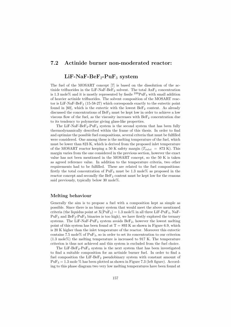
7.2 Actinide burner non-moderated reactor:

LiF-NaF-BeF2-PuF3 system

The fuel of the MOSART concept [7] is based on the dissolution of the ac-tinide trifluorides in the LiF-NaF-BeF2 solvent. The total AnF3 concentrationis 1.3 mole% and it is mostly represented by fissile 239PuF3 with small additionof heavier actinide trifluorides. The solvent composition of the MOSART reac-tor is LiF-NaF-BeF2 (15-58-27) which corresponds exactly to the eutectic pointfound in [60], which is the eutectic with the lowest BeF2 content. As alreadydiscussed the concentrations of BeF2 must be kept low in order to achieve a lowviscous flow of the fuel, as the viscosity increases with BeF2 concentration dueto its tendency to polymerize giving glass-like properties.

The LiF-NaF-BeF2-PuF3 system is the second system that has been fullythermodynamically described within the frame of this thesis. In order to findand optimize the possible fuel compositions, several criteria that must be fulfilledwere considered. One among these is the melting temperature of the fuel, whichmust be lower than 823 K, which is derived from the proposed inlet temperatureof the MOSART reactor keeping a 50 K safety margin (Tinlet = 873 K). Thismargin varies from the one considered in the previous section, however the exactvalue has not been mentioned in the MOSART concept, so the 50 K is takenas agreed reference value. In addition to the temperature criteria, two otherrequirements had to be fulfilled. These are related to the fuel compositions:firstly the total concentration of PuF3 must be 1.3 mole% as proposed in thereactor concept and secondly the BeF2 content must be kept low for the reasonssaid previously, typically below 30 mole%.

Melting behaviour

Generally the aim is to propose a fuel with a composition kept as simple aspossible. Since there is no binary system that would meet the above mentionedcriteria (the liquidus point at X(PuF3) = 1.3 mole% in all three LiF-PuF3, NaF-PuF3 and BeF2-PuF3 binaries is too high), we have firstly explored the ternarysystems. The LiF-NaF-PuF3 system avoids BeF2, however the lowest meltingpoint of this system has been found at T = 893 K as shown in Figure 6.9, whichis 20 K higher than the inlet temperature of the reactor. Moreover this eutecticcontains 7.5 mole% of PuF3, so in order to set its concentration to our criterion(1.3 mole%) the melting temperature is increased to 917 K. The temperaturecriterion is thus not achieved and this system is excluded from the fuel choice.

The LiF-BeF2-PuF3 system is the next system that has been investigatedto find a suitable composition for an actinide burner fuel. In order to find afuel composition the LiF-BeF2 pseudobinary system with constant amount ofPuF3 = 1.3 mole % has been plotted as shown in Figure 7.3 (left figure). Accord-ing to this phase diagram two very low melting temperatures have been found at

157

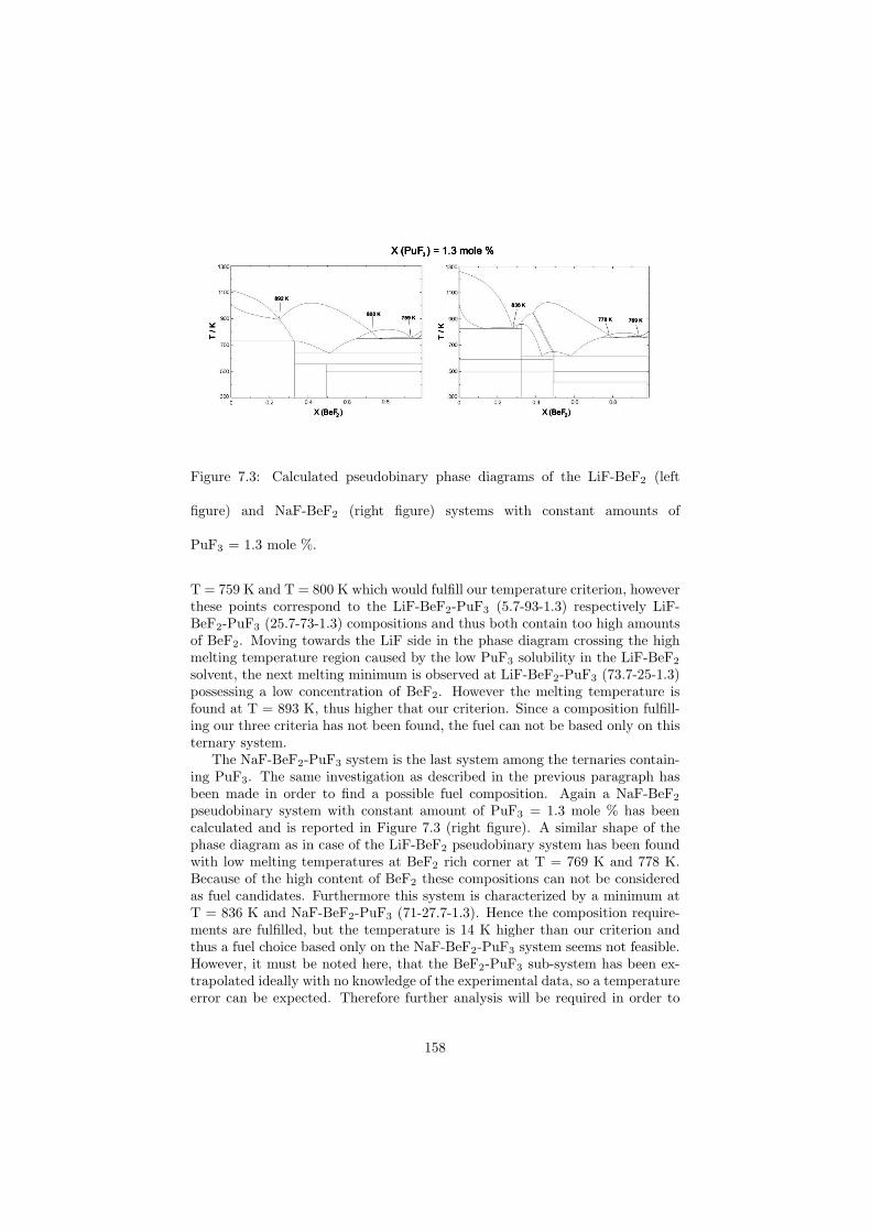
Figure 7.3: Calculated pseudobinary phase diagrams of the LiF-BeF2 (left

figure) and NaF-BeF2 (right figure) systems with constant amounts of

PuF3 = 1.3 mole %.

T = 759 K and T = 800 K which would fulfill our temperature criterion, howeverthese points correspond to the LiF-BeF2-PuF3 (5.7-93-1.3) respectively LiF-BeF2-PuF3 (25.7-73-1.3) compositions and thus both contain too high amountsof BeF2. Moving towards the LiF side in the phase diagram crossing the highmelting temperature region caused by the low PuF3 solubility in the LiF-BeF2

solvent, the next melting minimum is observed at LiF-BeF2-PuF3 (73.7-25-1.3)possessing a low concentration of BeF2. However the melting temperature isfound at T = 893 K, thus higher that our criterion. Since a composition fulfill-ing our three criteria has not been found, the fuel can not be based only on thisternary system.

The NaF-BeF2-PuF3 system is the last system among the ternaries contain-ing PuF3. The same investigation as described in the previous paragraph hasbeen made in order to find a possible fuel composition. Again a NaF-BeF2

pseudobinary system with constant amount of PuF3 = 1.3 mole % has beencalculated and is reported in Figure 7.3 (right figure). A similar shape of thephase diagram as in case of the LiF-BeF2 pseudobinary system has been foundwith low melting temperatures at BeF2 rich corner at T = 769 K and 778 K.Because of the high content of BeF2 these compositions can not be consideredas fuel candidates. Furthermore this system is characterized by a minimum atT = 836 K and NaF-BeF2-PuF3 (71-27.7-1.3). Hence the composition require-ments are fulfilled, but the temperature is 14 K higher than our criterion andthus a fuel choice based only on the NaF-BeF2-PuF3 system seems not feasible.However, it must be noted here, that the BeF2-PuF3 sub-system has been ex-trapolated ideally with no knowledge of the experimental data, so a temperatureerror can be expected. Therefore further analysis will be required in order to

158

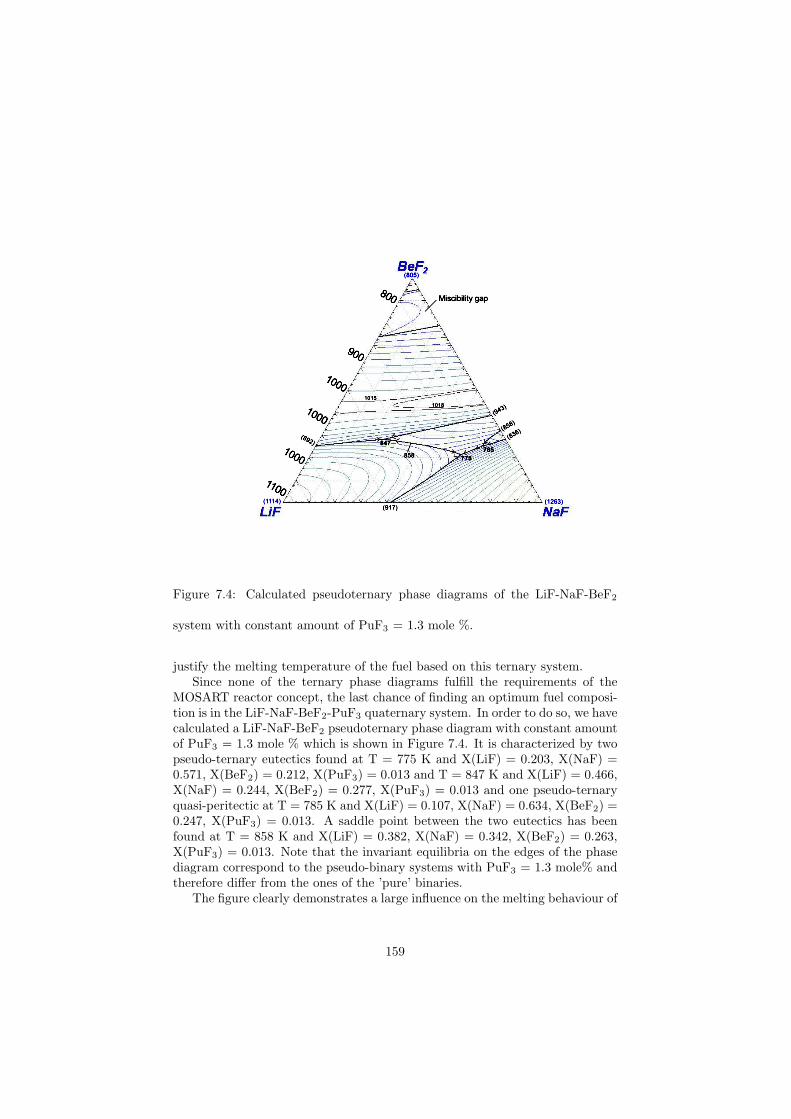
Figure 7.4: Calculated pseudoternary phase diagrams of the LiF-NaF-BeF2

system with constant amount of PuF3 = 1.3 mole %.

justify the melting temperature of the fuel based on this ternary system.Since none of the ternary phase diagrams fulfill the requirements of the

MOSART reactor concept, the last chance of finding an optimum fuel composi-tion is in the LiF-NaF-BeF2-PuF3 quaternary system. In order to do so, we havecalculated a LiF-NaF-BeF2 pseudoternary phase diagram with constant amountof PuF3 = 1.3 mole % which is shown in Figure 7.4. It is characterized by twopseudo-ternary eutectics found at T = 775 K and X(LiF) = 0.203, X(NaF) =0.571, X(BeF2) = 0.212, X(PuF3) = 0.013 and T = 847 K and X(LiF) = 0.466,X(NaF) = 0.244, X(BeF2) = 0.277, X(PuF3) = 0.013 and one pseudo-ternaryquasi-peritectic at T = 785 K and X(LiF) = 0.107, X(NaF) = 0.634, X(BeF2) =0.247, X(PuF3) = 0.013. A saddle point between the two eutectics has beenfound at T = 858 K and X(LiF) = 0.382, X(NaF) = 0.342, X(BeF2) = 0.263,X(PuF3) = 0.013. Note that the invariant equilibria on the edges of the phasediagram correspond to the pseudo-binary systems with PuF3 = 1.3 mole% andtherefore differ from the ones of the ’pure’ binaries.

The figure clearly demonstrates a large influence on the melting behaviour of

159

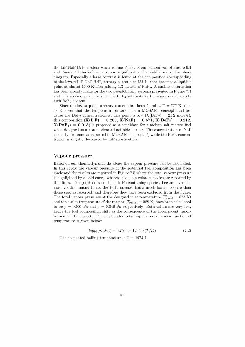
the LiF-NaF-BeF2 system when adding PuF3. From comparison of Figure 6.3and Figure 7.4 this influence is most significant in the middle part of the phasediagram. Especially a large contrast is found at the composition correspondingto the lowest LiF-NaF-BeF2 ternary eutectic at 553 K, that becomes a liquiduspoint at almost 1000 K after adding 1.3 mole% of PuF3. A similar observationhas been already made for the two pseudobinary systems presented in Figure 7.3and it is a consequence of very low PuF3 solubility in the regions of relativelyhigh BeF2 content.

Since the lowest pseudoternary eutectic has been found at T = 777 K, thus48 K lower that the temperature criterion for a MOSART concept, and be-cause the BeF2 concentration at this point is low (X(BeF2) = 21.2 mole%),this composition (X(LiF) = 0.203, X(NaF) = 0.571, X(BeF2) = 0.212,X(PuF3) = 0.013) is proposed as a candidate for a molten salt reactor fuelwhen designed as a non-moderated actinide burner. The concentration of NaFis nearly the same as reported in MOSART concept [7] while the BeF2 concen-tration is slightly decreased by LiF substitution.

Vapour pressure

Based on our thermodynamic database the vapour pressure can be calculated.In this study the vapour pressure of the potential fuel composition has beenmade and the results are reported in Figure 7.5 where the total vapour pressureis highlighted by a bold curve, whereas the most volatile species are reported bythin lines. The graph does not include Pu containing species, because even themost volatile among these, the PuF4 species, has a much lower pressure thanthose species reported, and therefore they have been excluded from the figure.The total vapour pressures at the designed inlet temperature (Tinlet = 873 K)and the outlet temperature of the reactor (Toutlet = 988 K) have been calculatedto be p = 0.001 Pa and p = 0.046 Pa respectively. Both values are very low,hence the fuel composition shift as the consequence of the incongruent vapor-ization can be neglected. The calculated total vapour pressure as a function oftemperature is given below:

log10(p/atm) = 6.7514− 12940/(T/K) (7.2)

The calculated boiling temperature is T = 1973 K.

160

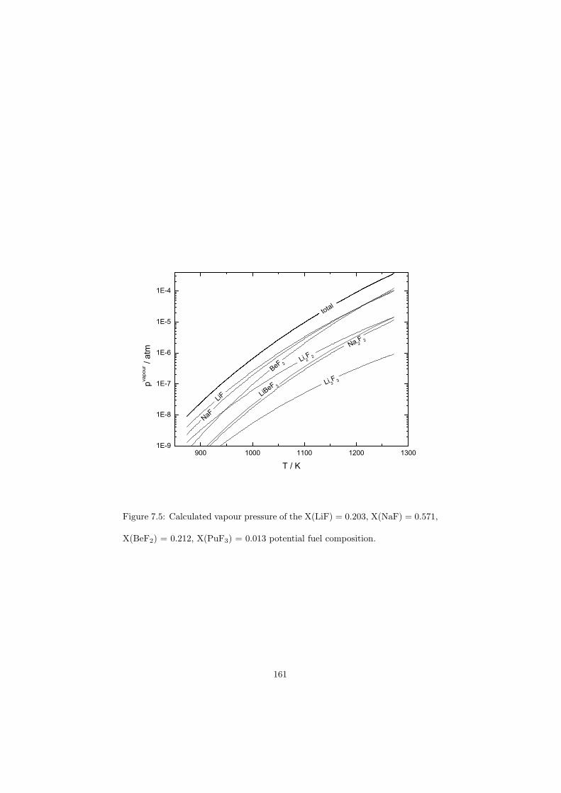
900 1000 1100 1200 13001E-9

1E-8

1E-7

1E-6

1E-5

1E-4

pva

po

ur /

atm

T / K

total

LiF

NaF

BeF 2Li 2

F 2

LiBeF 3

Na 2F 2

Li 3F 3

Figure 7.5: Calculated vapour pressure of the X(LiF) = 0.203, X(NaF) = 0.571,

X(BeF2) = 0.212, X(PuF3) = 0.013 potential fuel composition.

161

7.3 Actinide burner non-moderated reactor:

LiF-NaF-KF-RbF-(CsF)-PuF3 system

As discussed earlier the main interest of investigating the LiF-NaF-KF-RbF-CsF-PuF3 system is to avoid BeF2 from the fuel matrix which is based on theMOSART reactor concept [7]. It has been shown in the previous section thataccording to the melting requirements of the concept the fuel based only onthe LiF-NaF-PuF3 system can not be considered. Therefore the KF and RbFcompounds were taken as the candidates for BeF2 substitution. This choicewas possible since the MOSART concept is based on a non-moderated neutronspectrum in which the neutron capture cross section of the K and Rb atoms islow.

In order to search for a fuel alternative for the reactor based on the MOSARTconcept the same temperature and composition requirements as considered inthe previous section were kept in this case. Thus the melting temperature mustbe lower than 823 K and the concentration of PuF3 must be 1.3 mole%. SinceBeF2 is not considered in this system its concentration criteria are excluded.

Melting behaviour

There are six ternary phase diagrams containing PuF3 in the LiF-NaF-KF-RbF-PuF3 system. All of them are shown in Figures 6.9, 7.6, 7.7, 7.8, 7.9and 7.10 and their calculated invariant equilibria are listed in Table 7.1. As itcan be seen, four of these (LiF-KF-PuF3, LiF-RbF-PuF3, NaF-RbF-PuF3 andKF-RbF-PuF3) systems have eutectics lower than our criterion (T = 823 K).However the compositions of PuF3 in these systems are different from the tar-geted 1.3 mole%. Therefore a set of four pseudobinary phase diagrams hasbeen calculated keeping the concentration of PuF3 at 1.3 mole%. While in theKF-RbF-(PuF3 = 1.3 mole%) and NaF-RbF-(PuF3 = 1.3 mole%) systems thelowest melting temperatures are much too high to be acceptable for the moltensalt reactor (T = 1037 K and T = 935 K respectively), the other two LiF-KF-(PuF3 = 1.3 mole%) and LiF-RbF-(PuF3 = 1.3 mole%) systems fulfill thiscondition and can be considered as an actinide burner fuel. The lowest meltingpoints of these two systems correspond to X(LiF) = 0.482, X(KF) = 0.505,X(PuF3) = 0.013 and T = 760 K and X(LiF) = 0.439, X(RbF) = 0.548,X(PuF3) = 0.013 and T = 744 K respectively. Both compositions are reportedin Table 7.3.

It is also of interest to find the potential fuel compositions containing threecompounds of the matrix. Therefore further calculations have been made and itwas found that a matrix based on the ternary mixtures of LiF-NaF-RbF, LiF-NaF-KF and LiF-KF-RbF with addition of 1.3 mole% of PuF3 have very lowpseudo-ternary eutectics and these points can be considered as a fuel composi-tions also. The corresponding compositions and their melting points are given

162

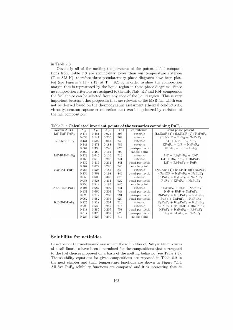
in Table 7.3.Obviously all of the melting temperatures of the potential fuel composi-

tions from Table 7.3 are significantly lower than our temperature criterion(T = 823 K), therefore three pseudoternary phase diagrams have been plot-ted (see Figures 7.11 - 7.13) at T = 823 K in order to show the compositionmargin that is represented by the liquid region in these phase diagrams. Sinceno composition criterions are assigned to the LiF, NaF, KF and RbF compoundsthe fuel choice can be selected from any spot of the liquid region. This is veryimportant because other properties that are relevant to the MSR fuel which cannot be derived based on the thermodynamic assessment (thermal conductivity,viscosity, neutron capture cross section etc.) can be optimized by variation ofthe fuel composition.

Table 7.1: Calculated invariant points of the ternaries containing PuF3.system A-B-C XA XB XC T (K) equilibrium solid phase presentLiF-NaF-PuF3 0.474 0.451 0.075 893 eutectic (Li,Na)F (1)+(Li,Na)F (2)+NaPuF4

0.633 0.147 0.220 969 eutectic (Li,Na)F + PuF3 + NaPuF4

LiF-KF-PuF3 0.431 0.522 0.047 749 eutectic KF + LiF + K3PuF6

0.341 0.471 0.188 786 eutectic KPuF4 + LiF + K3PuF6

0.364 0.390 0.246 825 quasi-peritectic KPuF4 + LiF + PuF3

0.360 0.480 0.161 790 saddle pointLiF-RbF-PuF3 0.228 0.645 0.126 713 eutectic LiF + Rb3PuF6 + RbF

0.163 0.618 0.218 741 eutectic LiF + Rb3PuF6 + RbPuF4

0.332 0.416 0.252 841 quasi-peritectic LiF + RbPuF4 + PuF3

0.167 0.622 0.210 743 saddle pointNaF-KF-PuF3 0.285 0.528 0.187 840 eutectic (Na,K)F (1)+(Na,K)F (2)+NaPuF4

0.234 0.568 0.198 843 quasi-peritectic (Na,K)F + K3PuF6 + NaPuF4

0.053 0.608 0.340 878 eutectic KPuF4 + K3PuF6 + NaPuF4

0.058 0.528 0.414 922 quasi-peritectic PuF3 + KPuF4 + NaPuF4

0.258 0.549 0.193 845 saddle pointNaF-RbF-PuF3 0.104 0.687 0.209 741 eutectic Rb3PuF6 + RbF + NaPuF4

0.131 0.666 0.203 748 quasi-peritectic NaF + RbF + NaPuF4

0.023 0.717 0.260 791 quasi-peritectic RbPuF4 + Rb3PuF6 + NaPuF4

0.062 0.582 0.356 920 quasi-peritectic PuF3 + NaPuF4 + RbPuF4

KF-RbF-PuF3 0.225 0.512 0.264 713 eutectic K3PuF6 + Rb3PuF6 + RbPuF4

0.225 0.530 0.245 714 eutectic K3PuF6 + (K,Rb)F + Rb3PuF6

0.318 0.385 0.297 758 quasi-peritectic KPuF4 + K3PuF6 + RbPuF4

0.317 0.326 0.357 826 quasi-peritectic PuF3 + KPuF4 + RbPuF4

0.225 0.525 0.250 714 saddle point

Solubility for actinides

Based on our thermodynamic assessment the solubilities of PuF3 in the mixturesof alkali fluorides have been determined for the compositions that correspondto the fuel choices proposed on a basis of the melting behavior (see Table 7.3).The solubility equations for given compositions are reported in Table 8.2 inthe next chapter and their temperature functions are shown in Figure 7.14.All five PuF3 solubility functions are compared and it is interesting that at

163

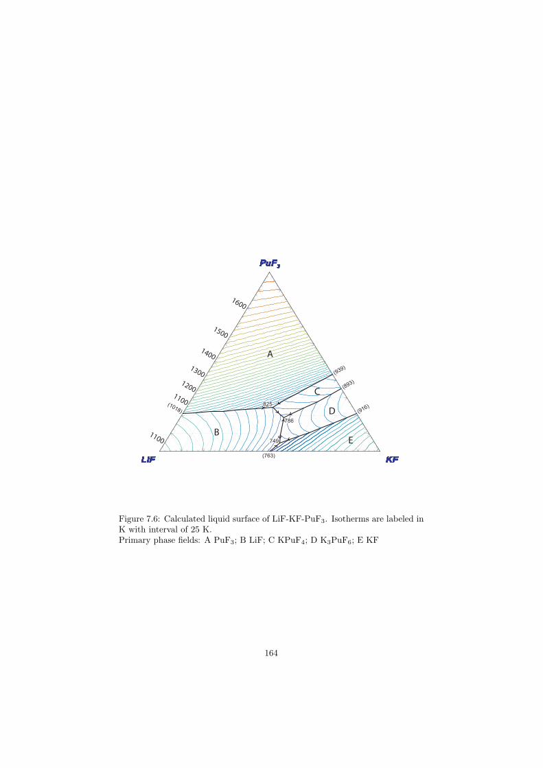
PuF3

LiF KFmole fractions /(PuF3+KF+LiF)

PuF3

LiF KFmole fractions /(PuF3+KF+LiF)

PuF3

LiF KFmole fractions /(PuF3+KF+LiF)

PuF3

LiF KFmole fractions /(PuF3+KF+LiF)

PuF3

LiF KFmole fractions /(PuF3+KF+LiF)

PuF3

LiF KFmole fractions /(PuF3+KF+LiF)

PuF3

LiF KFmole fractions /(PuF3+KF+LiF)

PuF3

LiF KFmole fractions /(PuF3+KF+LiF)

PuF3

LiF KFmole fractions /(PuF3+KF+LiF)

PuF3

LiF KFmole fractions /(PuF3+KF+LiF)

PuF3

LiF KFmole fractions /(PuF3+KF+LiF)

PuF3

LiF KFmole fractions /(PuF3+KF+LiF)

PuF3

LiF KFmole fractions /(PuF3+KF+LiF)

PuF3

LiF KFmole fractions /(PuF3+KF+LiF)

PuF3

LiF KFmole fractions /(PuF3+KF+LiF)

PuF3

LiF KFmole fractions /(PuF3+KF+LiF)

PuF3

LiF KFmole fractions /(PuF3+KF+LiF)

PuF3

LiF KFmole fractions /(PuF3+KF+LiF)

PuF3

LiF KFmole fractions /(PuF3+KF+LiF)

PuF3

LiF KFmole fractions /(PuF3+KF+LiF)

PuF3

LiF KFmole fractions /(PuF3+KF+LiF)

PuF3

LiF KFmole fractions /(PuF3+KF+LiF)

PuF3

LiF KFmole fractions /(PuF3+KF+LiF)

PuF3

LiF KFmole fractions /(PuF3+KF+LiF)

PuF3

LiF KFmole fractions /(PuF3+KF+LiF)

PuF3

LiF KFmole fractions /(PuF3+KF+LiF)

PuF3

LiF KFmole fractions /(PuF3+KF+LiF)

PuF3

LiF KFmole fractions /(PuF3+KF+LiF)

PuF3

LiF KFmole fractions /(PuF3+KF+LiF)

PuF3

LiF KFmole fractions /(PuF3+KF+LiF)

PuF3

LiF KFmole fractions /(PuF3+KF+LiF)

PuF3

LiF KFmole fractions /(PuF3+KF+LiF)

PuF3

LiF KFmole fractions /(PuF3+KF+LiF)

PuF3

LiF KFmole fractions /(PuF3+KF+LiF)

PuF3

LiF KFmole fractions /(PuF3+KF+LiF)

PuF3

LiF KFmole fractions /(PuF3+KF+LiF)

PuF3

LiF KFmole fractions /(PuF3+KF+LiF)

PuF3

LiF KFmole fractions /(PuF3+KF+LiF)

PuF3

LiF KFmole fractions /(PuF3+KF+LiF)

PuF3

LiF KFmole fractions /(PuF3+KF+LiF)

PuF3

LiF KFmole fractions /(PuF3+KF+LiF)

PuF3

LiF KFmole fractions /(PuF3+KF+LiF)

PuF3

LiF KFmole fractions /(PuF3+KF+LiF)

PuF3

LiF KFmole fractions /(PuF3+KF+LiF)

A

B

C

D

E

1600

1500

1400

1300

12001100

1100

(1018)

(763)

(916)

(893)

(939)

749

786

825

Figure 7.6: Calculated liquid surface of LiF-KF-PuF3. Isotherms are labeled inK with interval of 25 K.Primary phase fields: A PuF3; B LiF; C KPuF4; D K3PuF6; E KF

164

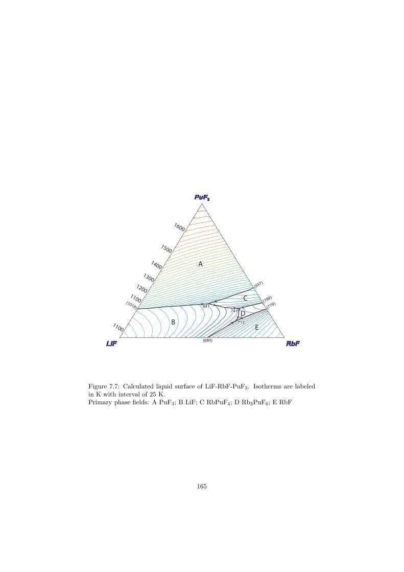
PuF3

LiF RbFmole fractions /(PuF3+RbF+LiF)

PuF3

LiF RbFmole fractions /(PuF3+RbF+LiF)

PuF3

LiF RbFmole fractions /(PuF3+RbF+LiF)

PuF3

LiF RbFmole fractions /(PuF3+RbF+LiF)

PuF3

LiF RbFmole fractions /(PuF3+RbF+LiF)

PuF3

LiF RbFmole fractions /(PuF3+RbF+LiF)

PuF3

LiF RbFmole fractions /(PuF3+RbF+LiF)

PuF3

LiF RbFmole fractions /(PuF3+RbF+LiF)

PuF3

LiF RbFmole fractions /(PuF3+RbF+LiF)

PuF3

LiF RbFmole fractions /(PuF3+RbF+LiF)

PuF3

LiF RbFmole fractions /(PuF3+RbF+LiF)

PuF3

LiF RbFmole fractions /(PuF3+RbF+LiF)

PuF3

LiF RbFmole fractions /(PuF3+RbF+LiF)

PuF3

LiF RbFmole fractions /(PuF3+RbF+LiF)

PuF3

LiF RbFmole fractions /(PuF3+RbF+LiF)

PuF3

LiF RbFmole fractions /(PuF3+RbF+LiF)

PuF3

LiF RbFmole fractions /(PuF3+RbF+LiF)

PuF3

LiF RbFmole fractions /(PuF3+RbF+LiF)

PuF3

LiF RbFmole fractions /(PuF3+RbF+LiF)

PuF3

LiF RbFmole fractions /(PuF3+RbF+LiF)

PuF3

LiF RbFmole fractions /(PuF3+RbF+LiF)

PuF3

LiF RbFmole fractions /(PuF3+RbF+LiF)

PuF3

LiF RbFmole fractions /(PuF3+RbF+LiF)

PuF3

LiF RbFmole fractions /(PuF3+RbF+LiF)

PuF3

LiF RbFmole fractions /(PuF3+RbF+LiF)

PuF3

LiF RbFmole fractions /(PuF3+RbF+LiF)

PuF3

LiF RbFmole fractions /(PuF3+RbF+LiF)

PuF3

LiF RbFmole fractions /(PuF3+RbF+LiF)

PuF3

LiF RbFmole fractions /(PuF3+RbF+LiF)

PuF3

LiF RbFmole fractions /(PuF3+RbF+LiF)

PuF3

LiF RbFmole fractions /(PuF3+RbF+LiF)

PuF3

LiF RbFmole fractions /(PuF3+RbF+LiF)

PuF3

LiF RbFmole fractions /(PuF3+RbF+LiF)

PuF3

LiF RbFmole fractions /(PuF3+RbF+LiF)

PuF3

LiF RbFmole fractions /(PuF3+RbF+LiF)

PuF3

LiF RbFmole fractions /(PuF3+RbF+LiF)

PuF3

LiF RbFmole fractions /(PuF3+RbF+LiF)

PuF3

LiF RbFmole fractions /(PuF3+RbF+LiF)

PuF3

LiF RbFmole fractions /(PuF3+RbF+LiF)

PuF3

LiF RbFmole fractions /(PuF3+RbF+LiF)

PuF3

LiF RbFmole fractions /(PuF3+RbF+LiF)

PuF3

LiF RbFmole fractions /(PuF3+RbF+LiF)

PuF3

LiF RbFmole fractions /(PuF3+RbF+LiF)

PuF3

LiF RbFmole fractions /(PuF3+RbF+LiF)

PuF3

LiF RbFmole fractions /(PuF3+RbF+LiF)

1600

1500

1400

1300

12001100

1100

A

B

C

D

E

(1018)

(680)

(779)

(799)

(937)

713

741

841

Figure 7.7: Calculated liquid surface of LiF-RbF-PuF3. Isotherms are labeledin K with interval of 25 K.Primary phase fields: A PuF3; B LiF; C RbPuF4; D Rb3PuF6; E RbF

165

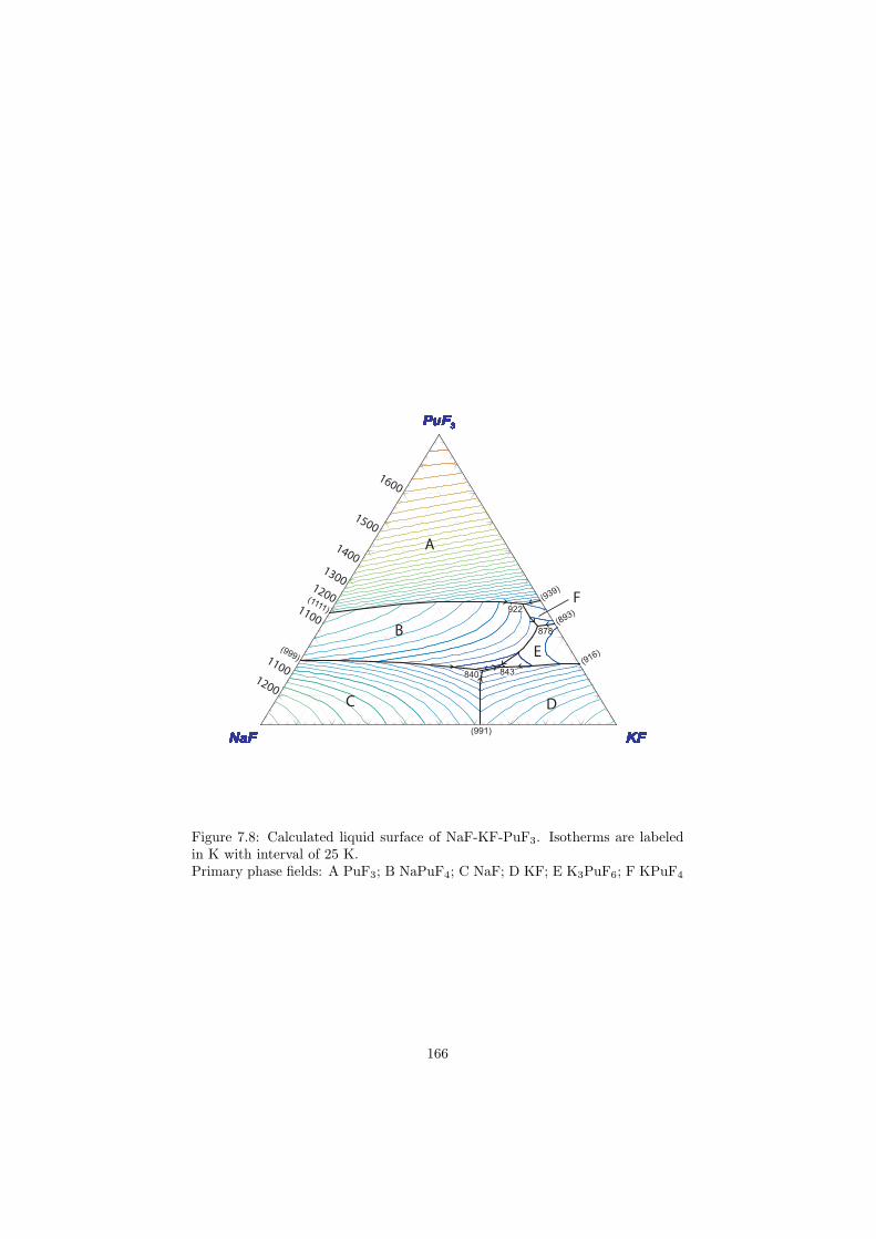
PuF3

NaF KFmole fractions /(PuF3+KF+NaF)

PuF3

NaF KFmole fractions /(PuF3+KF+NaF)

PuF3

NaF KFmole fractions /(PuF3+KF+NaF)

PuF3

NaF KFmole fractions /(PuF3+KF+NaF)

PuF3

NaF KFmole fractions /(PuF3+KF+NaF)

PuF3

NaF KFmole fractions /(PuF3+KF+NaF)

PuF3

NaF KFmole fractions /(PuF3+KF+NaF)

PuF3

NaF KFmole fractions /(PuF3+KF+NaF)

PuF3

NaF KFmole fractions /(PuF3+KF+NaF)

PuF3

NaF KFmole fractions /(PuF3+KF+NaF)

PuF3

NaF KFmole fractions /(PuF3+KF+NaF)

PuF3

NaF KFmole fractions /(PuF3+KF+NaF)

PuF3

NaF KFmole fractions /(PuF3+KF+NaF)

PuF3

NaF KFmole fractions /(PuF3+KF+NaF)

PuF3

NaF KFmole fractions /(PuF3+KF+NaF)

PuF3

NaF KFmole fractions /(PuF3+KF+NaF)

PuF3

NaF KFmole fractions /(PuF3+KF+NaF)

PuF3

NaF KFmole fractions /(PuF3+KF+NaF)

PuF3

NaF KFmole fractions /(PuF3+KF+NaF)

PuF3

NaF KFmole fractions /(PuF3+KF+NaF)

PuF3

NaF KFmole fractions /(PuF3+KF+NaF)

PuF3

NaF KFmole fractions /(PuF3+KF+NaF)

PuF3

NaF KFmole fractions /(PuF3+KF+NaF)

PuF3

NaF KFmole fractions /(PuF3+KF+NaF)

PuF3

NaF KFmole fractions /(PuF3+KF+NaF)

PuF3

NaF KFmole fractions /(PuF3+KF+NaF)

PuF3

NaF KFmole fractions /(PuF3+KF+NaF)

PuF3

NaF KFmole fractions /(PuF3+KF+NaF)

PuF3

NaF KFmole fractions /(PuF3+KF+NaF)

PuF3

NaF KFmole fractions /(PuF3+KF+NaF)

PuF3

NaF KFmole fractions /(PuF3+KF+NaF)

PuF3

NaF KFmole fractions /(PuF3+KF+NaF)

PuF3

NaF KFmole fractions /(PuF3+KF+NaF)

PuF3

NaF KFmole fractions /(PuF3+KF+NaF)

PuF3

NaF KFmole fractions /(PuF3+KF+NaF)

PuF3

NaF KFmole fractions /(PuF3+KF+NaF)

PuF3

NaF KFmole fractions /(PuF3+KF+NaF)

PuF3

NaF KFmole fractions /(PuF3+KF+NaF)

PuF3

NaF KFmole fractions /(PuF3+KF+NaF)

PuF3

NaF KFmole fractions /(PuF3+KF+NaF)

A

B

C D

E

F

1600

1500

1400

13001200

1100

11001200

840 843

878

922

(999)

(1111)

(916)

(893)

(939)

(991)

Figure 7.8: Calculated liquid surface of NaF-KF-PuF3. Isotherms are labeledin K with interval of 25 K.Primary phase fields: A PuF3; B NaPuF4; C NaF; D KF; E K3PuF6; F KPuF4

166

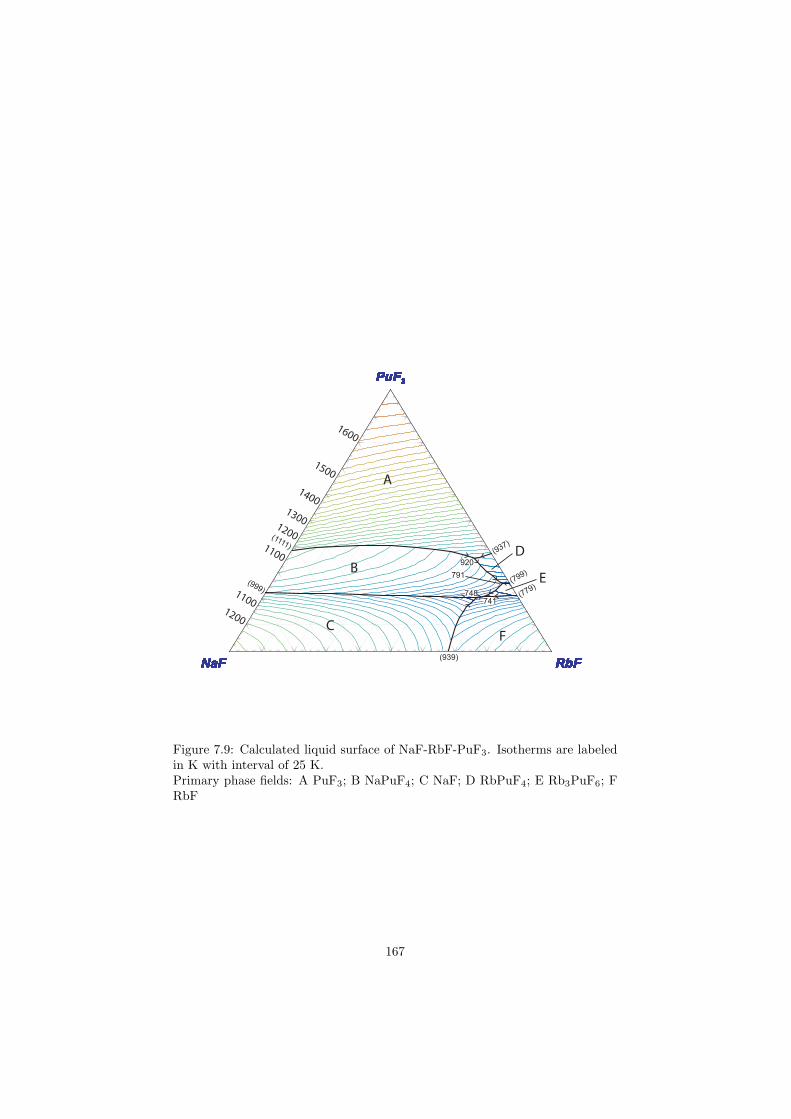
PuF3

NaF RbFmole fractions /(PuF3+RbF+NaF)

PuF3

NaF RbFmole fractions /(PuF3+RbF+NaF)

PuF3

NaF RbFmole fractions /(PuF3+RbF+NaF)

PuF3

NaF RbFmole fractions /(PuF3+RbF+NaF)

PuF3

NaF RbFmole fractions /(PuF3+RbF+NaF)

PuF3

NaF RbFmole fractions /(PuF3+RbF+NaF)

PuF3

NaF RbFmole fractions /(PuF3+RbF+NaF)

PuF3

NaF RbFmole fractions /(PuF3+RbF+NaF)

PuF3

NaF RbFmole fractions /(PuF3+RbF+NaF)

PuF3

NaF RbFmole fractions /(PuF3+RbF+NaF)

PuF3

NaF RbFmole fractions /(PuF3+RbF+NaF)

PuF3

NaF RbFmole fractions /(PuF3+RbF+NaF)

PuF3

NaF RbFmole fractions /(PuF3+RbF+NaF)

PuF3

NaF RbFmole fractions /(PuF3+RbF+NaF)

PuF3

NaF RbFmole fractions /(PuF3+RbF+NaF)

PuF3

NaF RbFmole fractions /(PuF3+RbF+NaF)

PuF3

NaF RbFmole fractions /(PuF3+RbF+NaF)

PuF3

NaF RbFmole fractions /(PuF3+RbF+NaF)

PuF3

NaF RbFmole fractions /(PuF3+RbF+NaF)

PuF3

NaF RbFmole fractions /(PuF3+RbF+NaF)

PuF3

NaF RbFmole fractions /(PuF3+RbF+NaF)

PuF3

NaF RbFmole fractions /(PuF3+RbF+NaF)

PuF3

NaF RbFmole fractions /(PuF3+RbF+NaF)

PuF3

NaF RbFmole fractions /(PuF3+RbF+NaF)

PuF3

NaF RbFmole fractions /(PuF3+RbF+NaF)

PuF3

NaF RbFmole fractions /(PuF3+RbF+NaF)

PuF3

NaF RbFmole fractions /(PuF3+RbF+NaF)

PuF3

NaF RbFmole fractions /(PuF3+RbF+NaF)

PuF3

NaF RbFmole fractions /(PuF3+RbF+NaF)

PuF3

NaF RbFmole fractions /(PuF3+RbF+NaF)

PuF3

NaF RbFmole fractions /(PuF3+RbF+NaF)

PuF3

NaF RbFmole fractions /(PuF3+RbF+NaF)

PuF3

NaF RbFmole fractions /(PuF3+RbF+NaF)

PuF3

NaF RbFmole fractions /(PuF3+RbF+NaF)

PuF3

NaF RbFmole fractions /(PuF3+RbF+NaF)

PuF3

NaF RbFmole fractions /(PuF3+RbF+NaF)

PuF3

NaF RbFmole fractions /(PuF3+RbF+NaF)

PuF3

NaF RbFmole fractions /(PuF3+RbF+NaF)

PuF3

NaF RbFmole fractions /(PuF3+RbF+NaF)

PuF3

NaF RbFmole fractions /(PuF3+RbF+NaF)

PuF3

NaF RbFmole fractions /(PuF3+RbF+NaF)

PuF3

NaF RbFmole fractions /(PuF3+RbF+NaF)

PuF3

NaF RbFmole fractions /(PuF3+RbF+NaF)

PuF3

NaF RbFmole fractions /(PuF3+RbF+NaF)

A

B

C

D

E

F

1600

1500

14001300

1200

1100

11001200

748

741

791

920

(779)

(799)

(937)

(999)

(1111)

(939)

Figure 7.9: Calculated liquid surface of NaF-RbF-PuF3. Isotherms are labeledin K with interval of 25 K.Primary phase fields: A PuF3; B NaPuF4; C NaF; D RbPuF4; E Rb3PuF6; FRbF

167

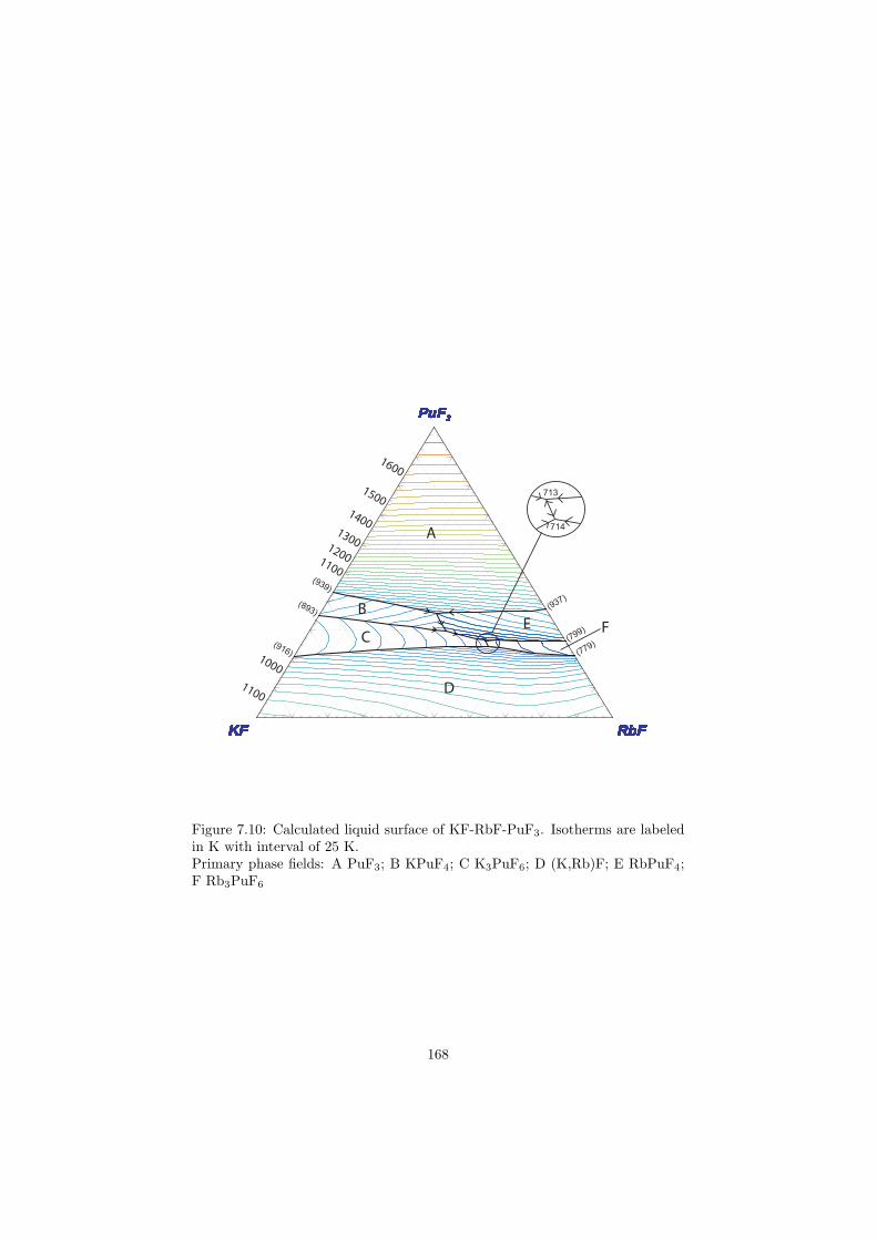
PuF3

KF RbFmole fractions /(PuF3+RbF+KF)

PuF3

KF RbFmole fractions /(PuF3+RbF+KF)

PuF3

KF RbFmole fractions /(PuF3+RbF+KF)

PuF3

KF RbFmole fractions /(PuF3+RbF+KF)

PuF3

KF RbFmole fractions /(PuF3+RbF+KF)

PuF3

KF RbFmole fractions /(PuF3+RbF+KF)

PuF3

KF RbFmole fractions /(PuF3+RbF+KF)

PuF3

KF RbFmole fractions /(PuF3+RbF+KF)

PuF3

KF RbFmole fractions /(PuF3+RbF+KF)

PuF3

KF RbFmole fractions /(PuF3+RbF+KF)

PuF3

KF RbFmole fractions /(PuF3+RbF+KF)

PuF3

KF RbFmole fractions /(PuF3+RbF+KF)

PuF3

KF RbFmole fractions /(PuF3+RbF+KF)

PuF3

KF RbFmole fractions /(PuF3+RbF+KF)

PuF3

KF RbFmole fractions /(PuF3+RbF+KF)

PuF3

KF RbFmole fractions /(PuF3+RbF+KF)

PuF3

KF RbFmole fractions /(PuF3+RbF+KF)

PuF3

KF RbFmole fractions /(PuF3+RbF+KF)

PuF3

KF RbFmole fractions /(PuF3+RbF+KF)

PuF3

KF RbFmole fractions /(PuF3+RbF+KF)

PuF3

KF RbFmole fractions /(PuF3+RbF+KF)

PuF3

KF RbFmole fractions /(PuF3+RbF+KF)

PuF3

KF RbFmole fractions /(PuF3+RbF+KF)

PuF3

KF RbFmole fractions /(PuF3+RbF+KF)

PuF3

KF RbFmole fractions /(PuF3+RbF+KF)

PuF3

KF RbFmole fractions /(PuF3+RbF+KF)

PuF3

KF RbFmole fractions /(PuF3+RbF+KF)

PuF3

KF RbFmole fractions /(PuF3+RbF+KF)

PuF3

KF RbFmole fractions /(PuF3+RbF+KF)

PuF3

KF RbFmole fractions /(PuF3+RbF+KF)

PuF3

KF RbFmole fractions /(PuF3+RbF+KF)

PuF3

KF RbFmole fractions /(PuF3+RbF+KF)

PuF3

KF RbFmole fractions /(PuF3+RbF+KF)

PuF3

KF RbFmole fractions /(PuF3+RbF+KF)

PuF3

KF RbFmole fractions /(PuF3+RbF+KF)

PuF3

KF RbFmole fractions /(PuF3+RbF+KF)

PuF3

KF RbFmole fractions /(PuF3+RbF+KF)

PuF3

KF RbFmole fractions /(PuF3+RbF+KF)

PuF3

KF RbFmole fractions /(PuF3+RbF+KF)

PuF3

KF RbFmole fractions /(PuF3+RbF+KF)

PuF3

KF RbFmole fractions /(PuF3+RbF+KF)

PuF3

KF RbFmole fractions /(PuF3+RbF+KF)

PuF3

KF RbFmole fractions /(PuF3+RbF+KF)

PuF3

KF RbFmole fractions /(PuF3+RbF+KF)

PuF3

KF RbFmole fractions /(PuF3+RbF+KF)

A

B

C

D

E F

1600

1500

14001300

12001100

1000

1100

713

714

(779)

(799)

(937)

(916)

(893)

(939)

Figure 7.10: Calculated liquid surface of KF-RbF-PuF3. Isotherms are labeledin K with interval of 25 K.Primary phase fields: A PuF3; B KPuF4; C K3PuF6; D (K,Rb)F; E RbPuF4;F Rb3PuF6

168

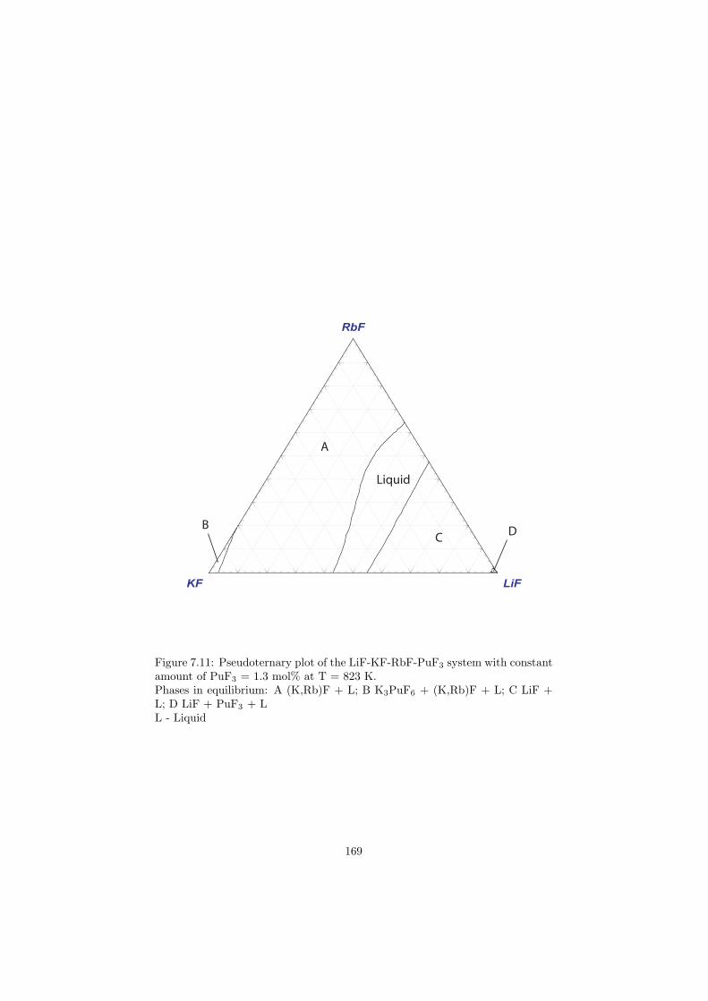
RbF

KF LiFmole fractions /(LiF+KF+RbF)

A

BC

D

Liquid

Figure 7.11: Pseudoternary plot of the LiF-KF-RbF-PuF3 system with constantamount of PuF3 = 1.3 mol% at T = 823 K.Phases in equilibrium: A (K,Rb)F + L; B K3PuF6 + (K,Rb)F + L; C LiF +L; D LiF + PuF3 + LL - Liquid

169

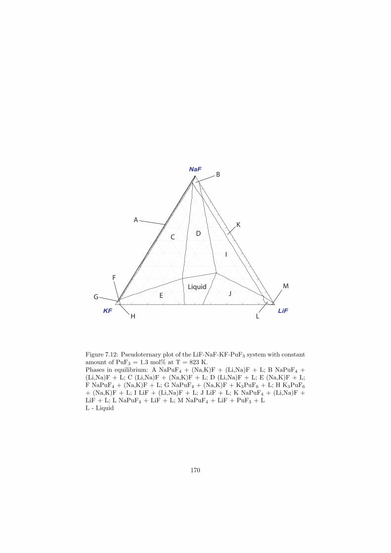
NaF

KF LiFmole fractions /(LiF+KF+NaF)

Liquid

A

B

CD

E

F

G

H

I

J

K

L

M

Figure 7.12: Pseudoternary plot of the LiF-NaF-KF-PuF3 system with constantamount of PuF3 = 1.3 mol% at T = 823 K.Phases in equilibrium: A NaPuF4 + (Na,K)F + (Li,Na)F + L; B NaPuF4 +(Li,Na)F + L; C (Li,Na)F + (Na,K)F + L; D (Li,Na)F + L; E (Na,K)F + L;F NaPuF4 + (Na,K)F + L; G NaPuF4 + (Na,K)F + K3PuF6 + L; H K3PuF6

+ (Na,K)F + L; I LiF + (Li,Na)F + L; J LiF + L; K NaPuF4 + (Li,Na)F +LiF + L; L NaPuF4 + LiF + L; M NaPuF4 + LiF + PuF3 + LL - Liquid

170

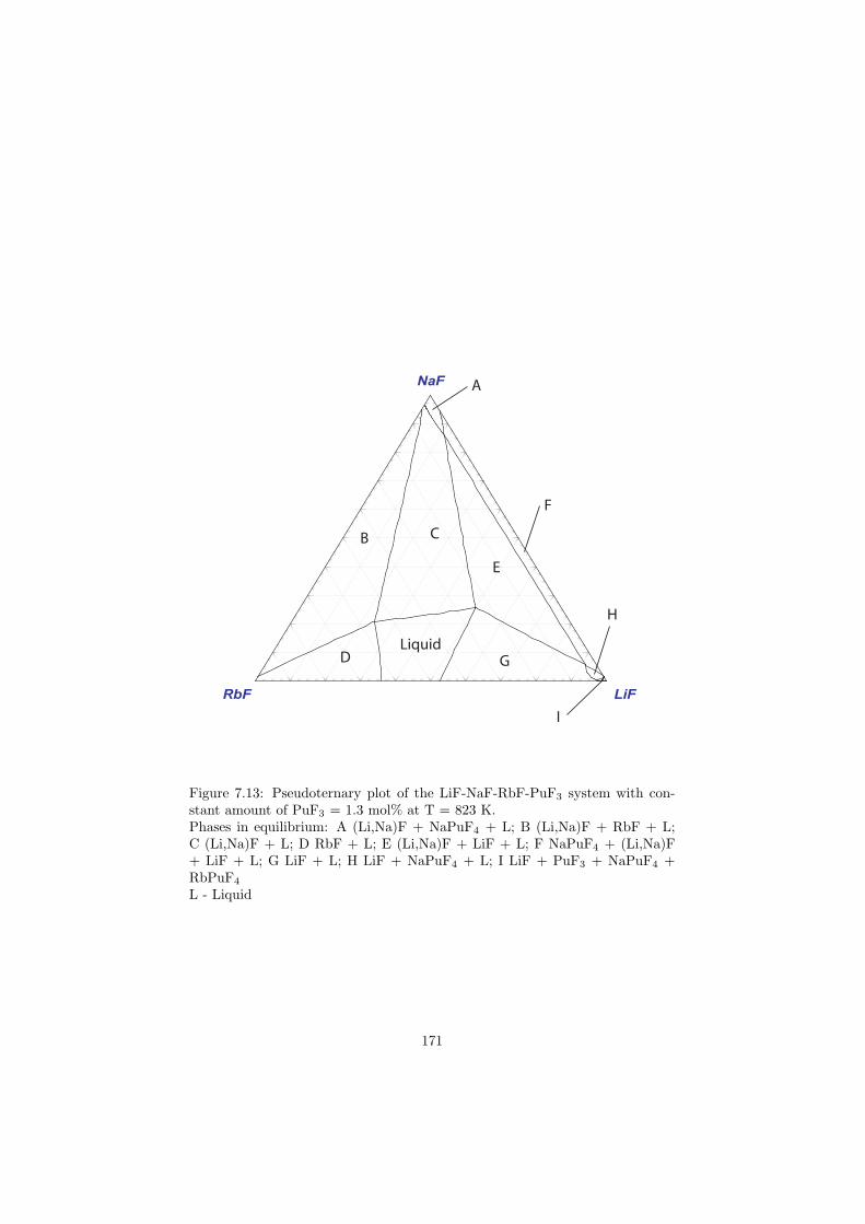
NaF

RbF LiFmole fractions /(LiF+RbF+NaF)

A

B C

DLiquid

E

F

G

H

I

Figure 7.13: Pseudoternary plot of the LiF-NaF-RbF-PuF3 system with con-stant amount of PuF3 = 1.3 mol% at T = 823 K.Phases in equilibrium: A (Li,Na)F + NaPuF4 + L; B (Li,Na)F + RbF + L;C (Li,Na)F + L; D RbF + L; E (Li,Na)F + LiF + L; F NaPuF4 + (Li,Na)F+ LiF + L; G LiF + L; H LiF + NaPuF4 + L; I LiF + PuF3 + NaPuF4 +RbPuF4

L - Liquid

171

higher temperatures (T > 940 K) the solubilities are similar in magnitude andare characterized by the same temperature dependence. In case of the LiF-NaF-RbF (0.400-0.142-0.458) matrix and the LiF-NaF-KF (0.439-0.142-0.419)matrix two different slopes have been observed on the solubility curve. This isexplained by the change of the primary crystallization field when increasing thePuF3 content. It is thus evident that these two compositions show lower PuF3

solubilities at the inlet temperature of the MOSART reactor compared to theother three compositions as indicated by the interaction with the vertical dottedline. Furthermore an interesting comparison has been made between the PuF3

solubility in the matrix of only alkali halides and in the matrix containing someaddition (27 mole%) of BeF2 as is the case of the fuel proposed in the MOSARTconcept [7]. It is shown that much lower values are obtained with some contentof BeF2. This observation has been also confirmed by Zherebtsov and Ignatievwho measured in their report [7] the influence of BeF2 concentration on thePuF3 solubility and found the same trend.

Another way to determine solubility is graphically shown in Figure 7.15.It is demonstrated for the PuF3 solubility in the matrix of LiF-KF (48.8-51.2mole%), which corresponds to one of our proposed fuel compositions. The figureshows an isothermal LiF-KF-PuF3 phase diagram constructed for T = 873 K,an inlet temperature of the MOSART reactor. The initial matrix compositionlies on the LiF-KF edge of the ternary phase diagram and is represented by Apoint, whereas the red solid line represents the initial LiF/KF ratio within thewhole phase diagram. Thus with increasing amount of PuF3 the compositionchanges along this line towards PuF3 corner. Since the liquidus line is a measureof solubility, as long as the red line belongs to the homogeneous liquid region,PuF3 is soluble. In our case the range of PuF3 solubility is represented by theAB section. Once the line crosses the liquidus border (B point in the figure),first solid precipitates appear and the solubility has its maximum here. The Bpoint corresponds to X(PuF3) = 0.268, thus the PuF3 solubility in the LiF-KF(48.8-51.2 mole%) matrix at T = 873 K is 26.8 mole%. It is exactly the samevalue as found from the equation from Table 8.2.

Vapor pressure

The vapour pressure of the five fuel candidates has been calculated for a temper-ature range 873 - 1273 K and the obtained results are reported in Figure 7.16.The figure clearly shows that the three fuel compositions that contain rela-tively high content of RbF, which is the most volatile compound in the matrixquadruplet, have higher vapour pressures than the compositions that are RbFfree. The vertical black dotted line represents the outlet temperature of thereactor and the vapour pressure values corresponding to that point, as reportedin Table 7.3, are around 3 Pa for RbF containing fuels and slightly below 1 Pafor the other two. The boiling temperatures of each of the fuel candidates havebeen determined as well and all are above 1800 K as reported in Table 8.1 inthe next chapter.

172

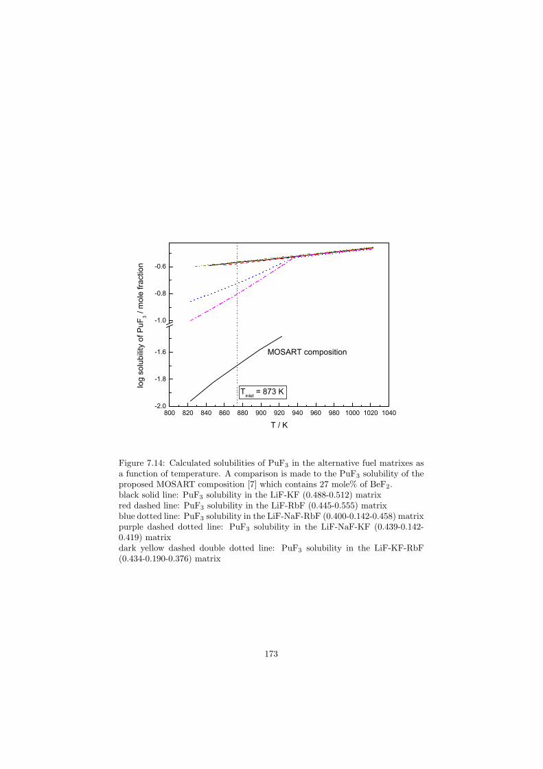
800 820 840 860 880 900 920 940 960 980 1000 1020 1040-2.0

-1.8

-1.6

-1.0

-0.8

-0.6

log

so

lub

ility

of P

uF

3 / m

ole

fra

ctio

n

T / K

Tinlet

= 873 K

MOSART composition

Figure 7.14: Calculated solubilities of PuF3 in the alternative fuel matrixes asa function of temperature. A comparison is made to the PuF3 solubility of theproposed MOSART composition [7] which contains 27 mole% of BeF2.black solid line: PuF3 solubility in the LiF-KF (0.488-0.512) matrixred dashed line: PuF3 solubility in the LiF-RbF (0.445-0.555) matrixblue dotted line: PuF3 solubility in the LiF-NaF-RbF (0.400-0.142-0.458) matrixpurple dashed dotted line: PuF3 solubility in the LiF-NaF-KF (0.439-0.142-0.419) matrixdark yellow dashed double dotted line: PuF3 solubility in the LiF-KF-RbF(0.434-0.190-0.376) matrix

173

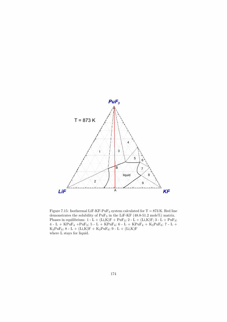
T = 873 K

A

B

liquid

1

2

3

4

56

7

8

9

Figure 7.15: Isothermal LiF-KF-PuF3 system calculated for T = 873 K. Red linedemonstrates the solubility of PuF3 in the LiF-KF (48.8-51.2 mole%) matrix.Phases in equilibrium: 1 - L + (Li,K)F + PuF3; 2 - L + (Li,K)F; 3 - L + PuF3;4 - L + KPuF4 +PuF3; 5 - L + KPuF4; 6 - L + KPuF4 + K3PuF6; 7 - L +K3PuF6; 8 - L + (Li,K)F + K3PuF6; 9 - L + (Li,K)Fwhere L stays for liquid.

174

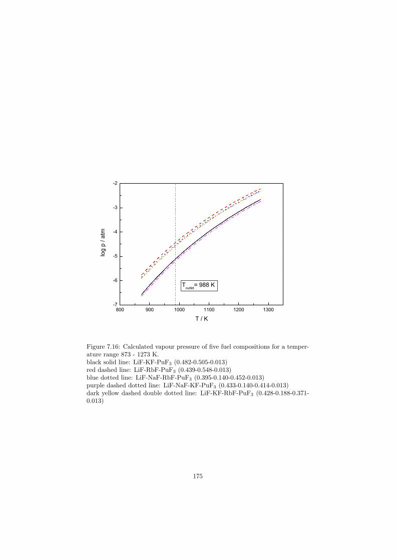
800 900 1000 1100 1200 1300-7

-6

-5

-4

-3

-2

log

p / a

tm

T / K

Toutlet

= 988 K

Figure 7.16: Calculated vapour pressure of five fuel compositions for a temper-ature range 873 - 1273 K.black solid line: LiF-KF-PuF3 (0.482-0.505-0.013)red dashed line: LiF-RbF-PuF3 (0.439-0.548-0.013)blue dotted line: LiF-NaF-RbF-PuF3 (0.395-0.140-0.452-0.013)purple dashed dotted line: LiF-NaF-KF-PuF3 (0.433-0.140-0.414-0.013)dark yellow dashed double dotted line: LiF-KF-RbF-PuF3 (0.428-0.188-0.371-0.013)

175

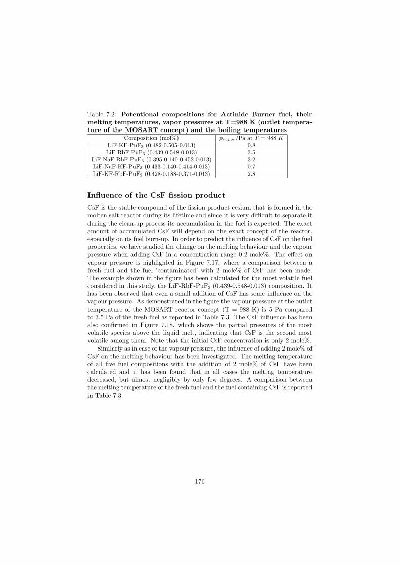
Table 7.2: Potentional compositions for Actinide Burner fuel, theirmelting temperatures, vapor pressures at T=988 K (outlet tempera-ture of the MOSART concept) and the boiling temperatures

Composition (mol%) pvapor/Pa at T = 988 K

LiF-KF-PuF3 (0.482-0.505-0.013) 0.8LiF-RbF-PuF3 (0.439-0.548-0.013) 3.5

LiF-NaF-RbF-PuF3 (0.395-0.140-0.452-0.013) 3.2LiF-NaF-KF-PuF3 (0.433-0.140-0.414-0.013) 0.7LiF-KF-RbF-PuF3 (0.428-0.188-0.371-0.013) 2.8

Influence of the CsF fission product

CsF is the stable compound of the fission product cesium that is formed in themolten salt reactor during its lifetime and since it is very difficult to separate itduring the clean-up process its accumulation in the fuel is expected. The exactamount of accumulated CsF will depend on the exact concept of the reactor,especially on its fuel burn-up. In order to predict the influence of CsF on the fuelproperties, we have studied the change on the melting behaviour and the vapourpressure when adding CsF in a concentration range 0-2 mole%. The effect onvapour pressure is highlighted in Figure 7.17, where a comparison between afresh fuel and the fuel ’contaminated’ with 2 mole% of CsF has been made.The example shown in the figure has been calculated for the most volatile fuelconsidered in this study, the LiF-RbF-PuF3 (0.439-0.548-0.013) composition. Ithas been observed that even a small addition of CsF has some influence on thevapour pressure. As demonstrated in the figure the vapour pressure at the outlettemperature of the MOSART reactor concept (T = 988 K) is 5 Pa comparedto 3.5 Pa of the fresh fuel as reported in Table 7.3. The CsF influence has beenalso confirmed in Figure 7.18, which shows the partial pressures of the mostvolatile species above the liquid melt, indicating that CsF is the second mostvolatile among them. Note that the initial CsF concentration is only 2 mole%.

Similarly as in case of the vapour pressure, the influence of adding 2 mole% ofCsF on the melting behaviour has been investigated. The melting temperatureof all five fuel compositions with the addition of 2 mole% of CsF have beencalculated and it has been found that in all cases the melting temperaturedecreased, but almost negligibly by only few degrees. A comparison betweenthe melting temperature of the fresh fuel and the fuel containing CsF is reportedin Table 7.3.

176

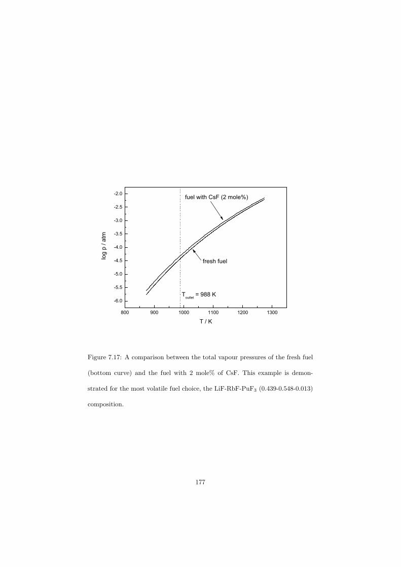
800 900 1000 1100 1200 1300

-6.0

-5.5

-5.0

-4.5

-4.0

-3.5

-3.0

-2.5

-2.0

log

p / a

tm

T / K

fuel with CsF (2 mole%)

Toutlet

= 988 K

fresh fuel

Figure 7.17: A comparison between the total vapour pressures of the fresh fuel

(bottom curve) and the fuel with 2 mole% of CsF. This example is demon-

strated for the most volatile fuel choice, the LiF-RbF-PuF3 (0.439-0.548-0.013)

composition.

177

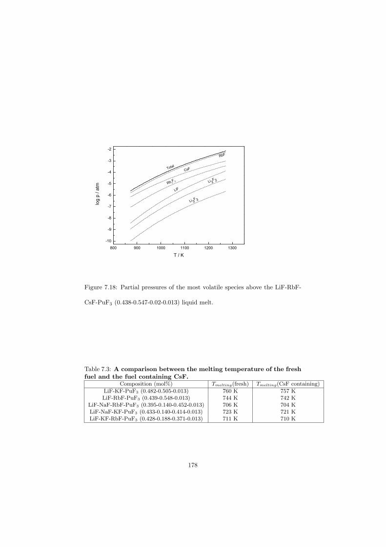
800 900 1000 1100 1200 1300

-10

-9

-8

-7

-6

-5

-4

-3

-2

Li 3F 3

log

p / a

tm

T / K

Total

RbF

CsF

Rb 2F 2

LiF

Li 2F 2

Figure 7.18: Partial pressures of the most volatile species above the LiF-RbF-

CsF-PuF3 (0.438-0.547-0.02-0.013) liquid melt.

Table 7.3: A comparison between the melting temperature of the freshfuel and the fuel containing CsF.

Composition (mol%) Tmelting(fresh) Tmelting(CsF containing)

LiF-KF-PuF3 (0.482-0.505-0.013) 760 K 757 KLiF-RbF-PuF3 (0.439-0.548-0.013) 744 K 742 K

LiF-NaF-RbF-PuF3 (0.395-0.140-0.452-0.013) 706 K 704 KLiF-NaF-KF-PuF3 (0.433-0.140-0.414-0.013) 723 K 721 KLiF-KF-RbF-PuF3 (0.428-0.188-0.371-0.013) 711 K 710 K

178

7.4 Molten salt fast breeder fuel:

NaCl-MgCl2-UCl3-PuCl3 system

Recently Mourogov and Bokov [13] proposed the fast breeder molten salt reactorREBUS-3700 based on a U-Pu cycle, where U and Pu are present in the form oftrichlorides dissolved in a matrix of liquid NaCl. In general the chlorides havehigher vapor pressures and lower thermodynamic stability at high temperaturescompared to fluorides, which are generally considered for molten salt reactorapplications [115], but on the other hand, they are less aggressive against thestructure materials and their melting points are lower. Therefore, more fissilematerial can be dissolved in the matrix and that is necessary for fast breederreactor designs. However, the chlorides can only be used in fast reactors andnot in thermal reactors, due to the relatively high parasitic neutron-capturecross-section of the chlorine atom.As already mentioned in the REBUS-3700 concept [13] NaCl serves as a matrixof the fuel, whereas 239PuCl3 is the fissile material and 238UCl3 is the fertilematerial. As a breeder design it produces more fissile material than it consumes.The mechanism is based on the neutron capture by 238U resulting in 239Pu. Forthe REBUS-3700 concept the proposed fresh fuel composition is 55 mol% NaCl,38 mol% UCl3 and 7 mol% PuCl3. The concentration of the actinide trichlorideshas been chosen in order to sustain the efficient chain reaction on the one handand to keep the positive breeding ratio on the other hand. Another importantfact that influences the fissile material concentration is the total amount ofchlorine, which is a neutron absorber, and the strategy of the fuel clean-up. Incase of REBUS-3700 it was proposed to have a continuous fuel clean-up with arate of 35 l/day [13].

Melting behaviour

In order to investigate the melting behaviour of the NaCl-UCl3-PuCl3 system,the ternary phase diagram has been assessed. It is shown in Figure 7.19 and ischaracterized by a single minimum on the Alkemade line which corresponds toT = 722 K, low enough to be suitable for a nuclear fuel. Nevertheless the com-position corresponding to this melting temperature was at X(NaCl) = 0.594,X(UCl3) = 0.045, X(PuCl3) = 0.360, for which the concentration of UCl3 istoo low and, on the contrary, the concentration of PuCl3 too high. Since themelting temperature found in our model was very low compared to our cri-terion (T = 873 K) there is sufficient margin for the melting temperature tooptimize the composition. Therefore, the isothermal plot at T = 873 K forthe NaCl-UCl3-PuCl3 system has been evaluated. It is reported in Figure 7.20where the dotted lines represent the constant concentrations of UCl3 and PuCl3at 38 mole% and 7 mole%, respectively. The intersection of these two linescorresponds exactly to the fuel proposal by REBUS-3700 and it can be seen

179

in Figure 7.20 that this point lies directly on the border of the liquid surface.Since T = 873 K is not the core inlet, but the lower temperature margin, thiscomposition is acceptable as a fuel for the MSR.

We studied in a further analysis the effect of MgCl2 on the NaCl-UCl3-PuCl3 system to see its influence on the melting behavior. The main aim ofthis study was to see if the melting temperature of the fuel decreases with thesubstitution of NaCl by MgCl2. The same procedure as described in the previousparagraph has been applied. First the lowest melting point, the quaternaryeutectic was calculated which was found at T = 697 K and X(NaCl) = 0.629,X(MgCl2) = 0.165, X(UCl3) = 0.011 and X(PuCl3) = 0.195. The temperatureis low enough to fulfill our criteria, but again, as in case of the NaCl-UCl3-PuCl3 system, the concentration of UCl3 is very low, while the concentration ofPuCl3 is rather high. Next, the isothermal pseudoternary phase diagram witha constant amount of PuCl3 of 7 mole% has been calculated for T = 873 K.This phase diagram is plotted in Figure 7.21, where the dotted line representsthe concentration of UCl3 equal to 38 mole% (in order to fulfill our criteria thefuel composition must be on this line). As it is obvious from the figure thisline intersects the liquid field at at the NaCl-UCl3 pseudobinary side (pointA in Figure 7.21), which means that the concentration of MgCl2 is zero andthe composition (point A) corresponds to X(NaCl) = 0.550, X(UCl3) = 0.380and X(PuCl3) = 0.070, the same composition as found in previous paragraph.This observation shows that the addition of MgCl2 to the NaCl-UCl3-PuCl3system, where UCl3 and PuCl3 are kept at 38 mole% and 7 mole%, respectively,increases its melting temperature. Thus it is not a good candidate to be usedas a component of the matrix for a fast breeder fuel based on the REBUS-3700concept.

Vapour pressure

The vapor pressure of the composition X(NaCl) = 0.550, X(UCl3) = 0.380,X(PuCl3) = 0.070 at T = 1003 K (the outlet temperature of REBUS-3700 reac-tor) has been calculated to be p = 2.54 Pa, thus relatively low and acceptable forthe MSR. The obtained total vapour pressure of the proposed fuel compositionas a function of temperature is given below:

log10(p/atm) = 5.434− 10065/(T/K) (7.3)

180

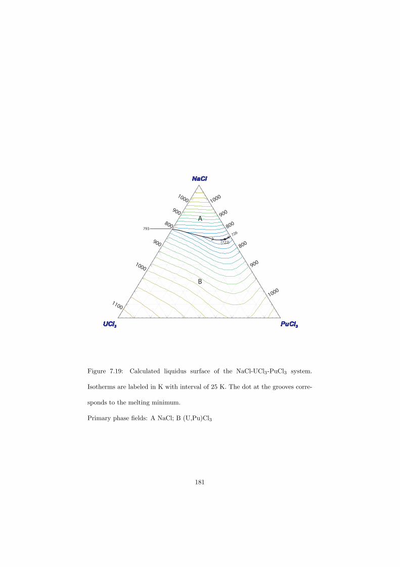
NaCl

UCl3

PuCl3

mole fraction

NaCl

UCl3

PuCl3

mole fraction

NaCl

UCl3

PuCl3

mole fraction

NaCl

UCl3

PuCl3

mole fraction

NaCl

UCl3

PuCl3

mole fraction

NaCl

UCl3

PuCl3

mole fraction

NaCl

UCl3

PuCl3

mole fraction

NaCl

UCl3

PuCl3

mole fraction

NaCl

UCl3

PuCl3

mole fraction

NaCl

UCl3

PuCl3

mole fraction

NaCl

UCl3

PuCl3

mole fraction

NaCl

UCl3

PuCl3

mole fraction

NaCl

UCl3

PuCl3

mole fraction

NaCl

UCl3

PuCl3

mole fraction

NaCl

UCl3

PuCl3

mole fraction

NaCl

UCl3

PuCl3

mole fraction

NaCl

UCl3

PuCl3

mole fraction

NaCl

UCl3

PuCl3

mole fraction

NaCl

UCl3

PuCl3

mole fraction

NaCl

UCl3

PuCl3

mole fraction

NaCl

UCl3

PuCl3

mole fraction

A

B

1000

900

800

900

1000

1100

1000

900

800

800

900

1000

(722)

726

793

Figure 7.19: Calculated liquidus surface of the NaCl-UCl3-PuCl3 system.

Isotherms are labeled in K with interval of 25 K. The dot at the grooves corre-

sponds to the melting minimum.

Primary phase fields: A NaCl; B (U,Pu)Cl3

181

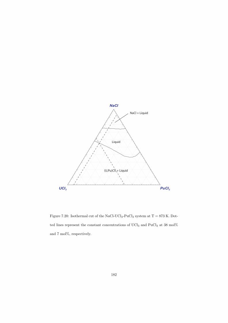
NaCl

UCl3

PuCl3

mole fractions /(NaCl+UCl3+PuCl3)

NaCl + Liquid

Liquid

(U,Pu)Cl3 + Liquid

Figure 7.20: Isothermal cut of the NaCl-UCl3-PuCl3 system at T = 873 K. Dot-

ted lines represent the constant concentrations of UCl3 and PuCl3 at 38 mol%

and 7 mol%, respectively.

182

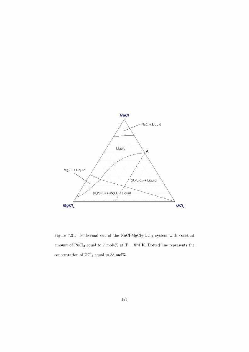
NaCl

MgCl2

UCl3

mole fractions /(NaCl+MgCl2+UCl3)

NaCl + Liquid

Liquid

MgCl2 + Liquid

(U,Pu)Cl3 + Liquid

(U,Pu)Cl3 + MgCl2 + Liquid

A

Figure 7.21: Isothermal cut of the NaCl-MgCl2-UCl3 system with constant

amount of PuCl3 equal to 7 mole% at T = 873 K. Dotted line represents the

concentration of UCl3 equal to 38 mol%.

183

Chapter 8

Conclusions and Summary

In this study a thermodynamic assessments of several systems that are of im-portance to the molten salt reactor project have been presented. Moreover someof the systems assessed are considered as good candidates for coolant choicesfor advanced high temperature reactors or the heat transfer salts for deliveringthe heat from the reactor core to the hydrogen power plant.

Since the basis of every thermodynamic assessment are the experimentaldata it was also a part of this study to make some new measurements thatwould improve the thermodynamic database created within the frame of thisstudy. It was a very challenging task to measure the fluoride systems up tohigh temperatures due to the corrosion effect of its vapour on the calorimeterdetector. Therefore it was necessary to develop an encapsulation technique thatwould avoid any vapour release above 1473 K on one hand while keeping goodsignal of the detector on the other. Two different methods for encapsulate of thefluoride samples have been developed for this purpose, one for the drop detectorthat was mainly used for the heat capacity measurements and the other for theDSC mode that was used to determine the equilibrium points of various phasediagrams.

The encapsulation technique for the drop calorimeter was first tested onthe heat capacity measurements of the (Li,Na)F liquid solution with successfulresults. Moreover based on this result it has been confirmed that the heatcapacity of the alkali fluorides behaves ideally, thus following the Neumann-Kopp rule. The encapsulation technique for the DSC detector was firstly testedon the measurement of the NaNO3-KNO3 system which is of interest in thenuclear research since it is one of the candidates proposed as a heat transfer saltfor a sodium cooled fast reactor. There exist two different version of this binaryso one of the tasks was to confirm which one is more likely the correct one.

184

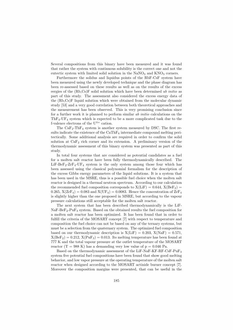
Several compositions from this binary have been measured and it was foundthat rather the system with continuous solubility is the correct one and not theeutectic system with limited solid solution in the NaNO3 and KNO3 corners.

Furthermore the solidus and liquidus points of the RbF-CsF system havebeen measured using the newly developed technique and the phase diagram hasbeen re-assessed based on these results as well as on the results of the excesseergies of the (Rb,Cs)F solid solution which have been determined ab initio aspart of this study. The assessment also considered the excess energy data ofthe (Rb,Cs)F liquid solution which were obtained from the molecular dynamicstudy [53] and a very good correlation between both theoretical approaches andthe measurement has been observed. This is very promising conclusion sincefor a further work it is planned to perform similar ab initio calculations on theThF4-UF4 system which is expected to be a more complicated task due to thef-valence electrons of the U4+ cation.

The CaF2-ThF4 system is another system measured by DSC. The first re-sults indicate the existence of the CaThF6 intermediate compound melting peri-tectically. Some additional analysis are required in order to confirm the solidsolution at CaF2 rich corner and its extension. A preliminary version of thethermodynamic assessment of this binary system was presented as part of thisstudy.

In total four systems that are considered as potential candidates as a fuelfor a molten salt reactor have been fully thermodynamically described. TheLiF-BeF2-ZrF4-UF4 system is the only system among those four which hasbeen assessed using the classical polynomial formalism for the description ofthe excess Gibbs energy parameters of the liquid solutions. It is a system thathas been used in the MSRE, thus is a possible fuel choice when the molten saltreactor is designed in a thermal neutron spectrum. According to our calculationthe recommended fuel composition corresponds to X(LiF) = 0.644, X(BeF2) =0.265, X(ZrF4) = 0.083 and X(UF4) = 0.0083. Hence the concentration of ZrF4

is slightly higher than the one proposed in MSRE, but according to the vapourpressure calculations still acceptable for the molten salt reactor.

The next system that has been described thermodynamically is the LiF-NaF-BeF2-PuF3 system. Based on the obtained results the fuel composition fora molten salt reactor has been optimized. It has been found that in order tofulfill the criteria of the MOSART concept [7] with respect to temperature andcomposition the fuel choice can not be based on any of the ternary systems, butmust be a selection from the quaternary system. The optimized fuel compositionbased on our thermodynamic description is X(LiF) = 0.203, X(NaF) = 0.571,X(BeF2) = 0.212, X(PuF3) = 0.013. Its melting temperature has been found at777 K and the total vapour pressure at the outlet temperature of the MOSARTreactor (T = 988 K) has a demanding very low value of p = 0.046 Pa.

Based on the thermodynamic assessment of the LiF-NaF-KF-RF-CsF-PuF3

system five potential fuel compositions have been found that show good meltingbehavior, and low vapor pressure at the operating temperature of the molten saltreactor when designed according to the MOSART actinide burner concept [7].Moreover the composition margins were presented, that can be useful in the

185

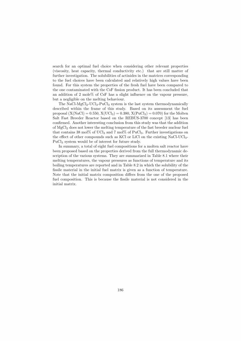
search for an optimal fuel choice when considering other relevant properties(viscosity, heat capacity, thermal conductivity etc.) that are still matter offurther investigation. The solubilities of actinides in the matrices correspondingto the fuel choices have been calculated and relatively high values have beenfound. For this system the properties of the fresh fuel have been compared tothe one contaminated with the CsF fission product. It has been concluded thatan addition of 2 mole% of CsF has a slight influence on the vapour pressure,but a negligible on the melting behaviour.

The NaCl-MgCl2-UCl3-PuCl3 system is the last system thermodynamicallydescribed within the frame of this study. Based on its assessment the fuelproposal (X(NaCl) = 0.550, X(UCl3) = 0.380, X(PuCl3) = 0.070) for the MoltenSalt Fast Breeder Reactor based on the REBUS-3700 concept [13] has beenconfirmed. Another interesting conclusion from this study was that the additionof MgCl2 does not lower the melting temperature of the fast breeder nuclear fuelthat contains 38 mol% of UCl3 and 7 mol% of PuCl3. Further investigations onthe effect of other compounds such as KCl or LiCl on the existing NaCl-UCl3-PuCl3 system would be of interest for future study.

In summary, a total of eight fuel compositions for a molten salt reactor havebeen proposed based on the properties derived from the full thermodynamic de-scription of the various systems. They are summarized in Table 8.1 where theirmelting temperatures, the vapour pressures as functions of temperature and itsboiling temperatures are reported and in Table 8.2 in which the solubility of thefissile material in the initial fuel matrix is given as a function of temperature.Note that the initial matrix composition differs from the one of the proposedfuel composition. This is because the fissile material is not considered in theinitial matrix.

186

Table 8.1: The various properties of the fuel choices made according to the thermodynamic database assessedin this study.

Fuel composition reactor type Melting temperature Vapour pressure Boiling temperature(mole%) (log p / atm)

LiF-BeF2-ZrF4-UF4 Thermal spectrum 706 K 6.2998 - 10546/(T/K) 1708 K(64.4-26.5-8.3-0.83)

LiF-NaF-BeF2-PuF3 Non-moderated burner 777 K 6.7514 - 12940/(T/K) 1973 K(20.3-57.1-21.2-1.3)

LiF-KF-PuF3 Non-moderated burner 760 K 5.840 - 10809/(T/K) 1918 K(0.482-0.505-0.013)

LiF-RbF-PuF3 Non-moderated burner 744 K 5.520 - 9827/(T/K) 1839 K(0.439-0.548-0.013)

LiF-NaF-RbF-PuF3 Non-moderated burner 706 K 5.429 - 9819/(T/K) 1866 K(0.395-0.140-0.452-0.013)

LiF-NaF-KF-PuF3 Non-moderated burner 723 K 5.790 - 10833/(T/K) 1937 K(0.433-0.140-0.414-0.013)

LiF-KF-RbF-PuF3 Non-moderated burner 711 K 5.486 - 9925/(T/K) 1863 K(0.428-0.188-0.371-0.013)

NaCl-UCl3-PuCl3 Fast breeder 873 K 5.434 - 10065/(T/K) 1913 K(0.550-0.380-0.070)

187

Table 8.2: Calculated solubility of PuF3 in the mixtures of given initial composition.Matrix composition (mole fraction) Solubility (mole fraction) Temperature range (K)

LiF-BeF2-ZrF4 (0.649-0.267-0.084) log10S = -9.359 + 1.799·10−2·T - 9.1468·10−6

·T2 723 - 883

LiF-NaF-BeF2 (0.206-0.579-0.215) log10S = -4.437 + 3.396·10−3·T 823 - 1023

LiF-KF (0.488-0.512) log10S = -1.211 + 0.733·10−3·T 843 - 1023

LiF-RbF (0.445-0.555) log10S = 53.144 - 1.3615·10−1·T + 8.541·10−5

·T2 823 - 859log10S = -1.253 + 7.727·10−4

·T 859 - 1023

LiF-NaF-RbF (0.400-0.142-0.458) log10S = 1.391 - 7.680·10−3·T + 6.016·10−6

·T2 823 - 933log10S = -1.246 + 7.587·10−4

·T 933 - 1023

LiF-NaF-KF (0.439-0.142-0.419) log10S = -1.416 - 2.670·10−3·T + 3.859·10−6

·T2 823 - 938log10S = -1.160 + 6.768·10−4

·T 938 - 1023

LiF-KF-RbF (0.434-0.190-0.376) log10S = -1.209 + 7.366·10−4·T 828 - 1023

NaCl-UCl3 (0.591-0.409) log10S = 46.894 - 1.296·10−1·T + 8.556·10−5

·T2 883 - 903

188

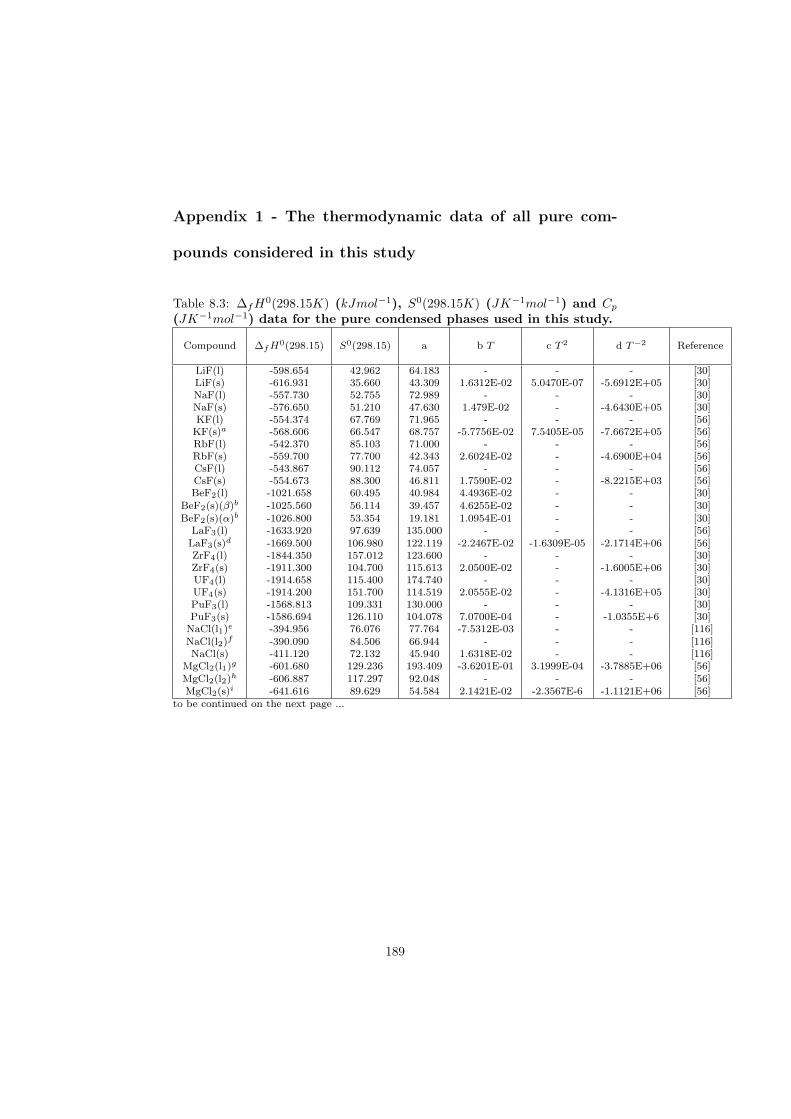
Appendix 1 - The thermodynamic data of all pure com-

pounds considered in this study

Table 8.3: ∆fH0(298.15K) (kJmol−1), S0(298.15K) (JK−1mol−1) and Cp

(JK−1mol−1) data for the pure condensed phases used in this study.

Compound ∆f H0(298.15) S0(298.15) a b T c T 2 d T−2 Reference

LiF(l) -598.654 42.962 64.183 - - - [30]LiF(s) -616.931 35.660 43.309 1.6312E-02 5.0470E-07 -5.6912E+05 [30]NaF(l) -557.730 52.755 72.989 - - - [30]NaF(s) -576.650 51.210 47.630 1.479E-02 - -4.6430E+05 [30]KF(l) -554.374 67.769 71.965 - - - [56]KF(s)a -568.606 66.547 68.757 -5.7756E-02 7.5405E-05 -7.6672E+05 [56]RbF(l) -542.370 85.103 71.000 - - - [56]RbF(s) -559.700 77.700 42.343 2.6024E-02 - -4.6900E+04 [56]CsF(l) -543.867 90.112 74.057 - - - [56]CsF(s) -554.673 88.300 46.811 1.7590E-02 - -8.2215E+03 [56]BeF2(l) -1021.658 60.495 40.984 4.4936E-02 - - [30]

BeF2(s)(β)b -1025.560 56.114 39.457 4.6255E-02 - - [30]BeF2(s)(α)b -1026.800 53.354 19.181 1.0954E-01 - - [30]

LaF3(l) -1633.920 97.639 135.000 - - - [56]LaF3(s)d -1669.500 106.980 122.119 -2.2467E-02 -1.6309E-05 -2.1714E+06 [56]ZrF4(l) -1844.350 157.012 123.600 - - - [30]ZrF4(s) -1911.300 104.700 115.613 2.0500E-02 - -1.6005E+06 [30]UF4(l) -1914.658 115.400 174.740 - - - [30]UF4(s) -1914.200 151.700 114.519 2.0555E-02 - -4.1316E+05 [30]PuF3(l) -1568.813 109.331 130.000 - - - [30]PuF3(s) -1586.694 126.110 104.078 7.0700E-04 - -1.0355E+6 [30]

NaCl(l1)e -394.956 76.076 77.764 -7.5312E-03 - - [116]NaCl(l2)f -390.090 84.506 66.944 - - - [116]NaCl(s) -411.120 72.132 45.940 1.6318E-02 - - [116]

MgCl2(l1)g -601.680 129.236 193.409 -3.6201E-01 3.1999E-04 -3.7885E+06 [56]MgCl2(l2)h -606.887 117.297 92.048 - - - [56]MgCl2(s)i -641.616 89.629 54.584 2.1421E-02 -2.3567E-6 -1.1121E+06 [56]

to be continued on the next page ...

189

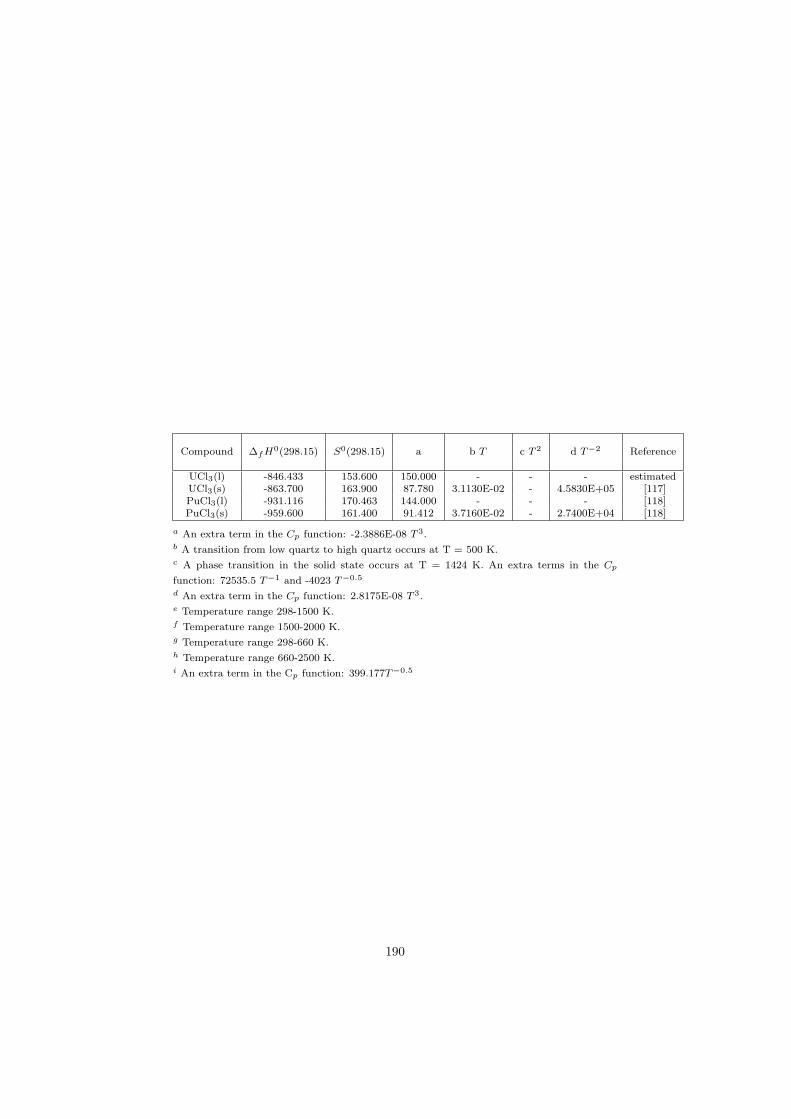
Compound ∆f H0(298.15) S0(298.15) a b T c T 2 d T−2 Reference

UCl3(l) -846.433 153.600 150.000 - - - estimatedUCl3(s) -863.700 163.900 87.780 3.1130E-02 - 4.5830E+05 [117]PuCl3(l) -931.116 170.463 144.000 - - - [118]PuCl3(s) -959.600 161.400 91.412 3.7160E-02 - 2.7400E+04 [118]

a An extra term in the Cp function: -2.3886E-08 T 3.b A transition from low quartz to high quartz occurs at T = 500 K.c A phase transition in the solid state occurs at T = 1424 K. An extra terms in the Cp

function: 72535.5 T−1 and -4023 T−0.5

d An extra term in the Cp function: 2.8175E-08 T 3.e Temperature range 298-1500 K.f Temperature range 1500-2000 K.g Temperature range 298-660 K.h Temperature range 660-2500 K.i An extra term in the Cp function: 399.177T−0.5

190

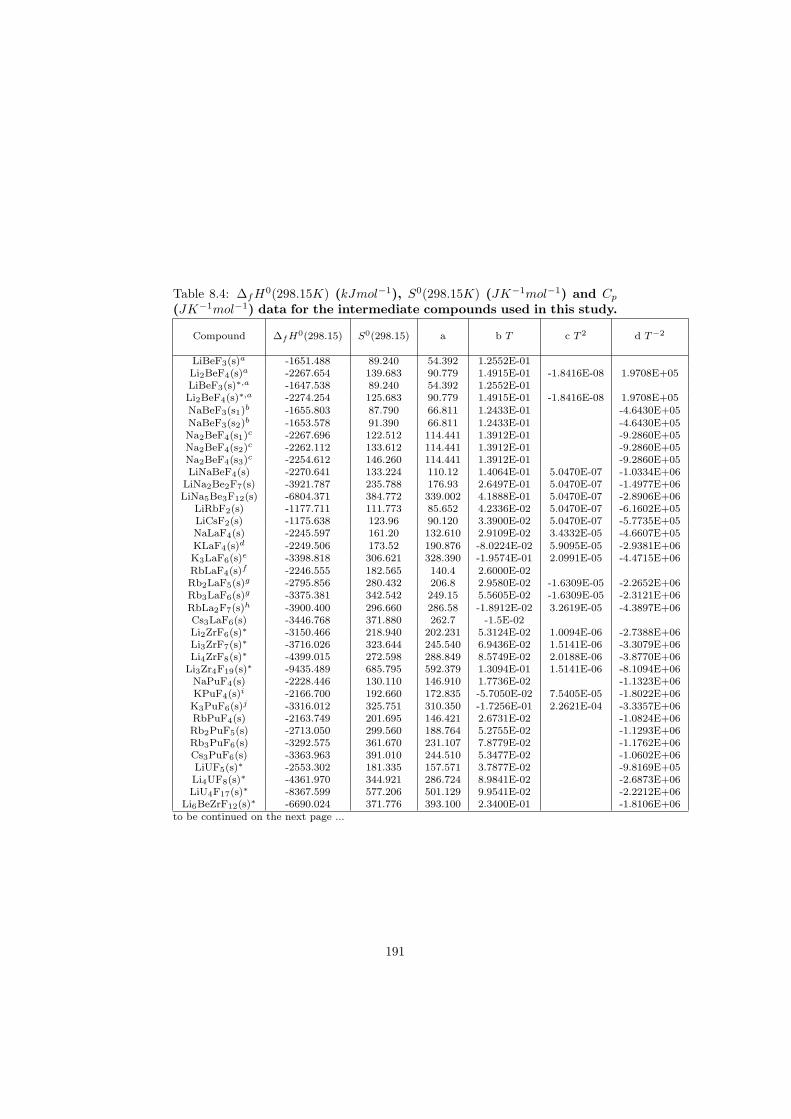
Table 8.4: ∆fH0(298.15K) (kJmol−1), S0(298.15K) (JK−1mol−1) and Cp

(JK−1mol−1) data for the intermediate compounds used in this study.

Compound ∆f H0(298.15) S0(298.15) a b T c T 2 d T−2

LiBeF3(s)a -1651.488 89.240 54.392 1.2552E-01Li2BeF4(s)a -2267.654 139.683 90.779 1.4915E-01 -1.8416E-08 1.9708E+05LiBeF3(s)∗,a -1647.538 89.240 54.392 1.2552E-01Li2BeF4(s)∗,a -2274.254 125.683 90.779 1.4915E-01 -1.8416E-08 1.9708E+05NaBeF3(s1)b -1655.803 87.790 66.811 1.2433E-01 -4.6430E+05NaBeF3(s2)b -1653.578 91.390 66.811 1.2433E-01 -4.6430E+05Na2BeF4(s1)c -2267.696 122.512 114.441 1.3912E-01 -9.2860E+05Na2BeF4(s2)c -2262.112 133.612 114.441 1.3912E-01 -9.2860E+05Na2BeF4(s3)c -2254.612 146.260 114.441 1.3912E-01 -9.2860E+05LiNaBeF4(s) -2270.641 133.224 110.12 1.4064E-01 5.0470E-07 -1.0334E+06

LiNa2Be2F7(s) -3921.787 235.788 176.93 2.6497E-01 5.0470E-07 -1.4977E+06LiNa5Be3F12(s) -6804.371 384.772 339.002 4.1888E-01 5.0470E-07 -2.8906E+06

LiRbF2(s) -1177.711 111.773 85.652 4.2336E-02 5.0470E-07 -6.1602E+05LiCsF2(s) -1175.638 123.96 90.120 3.3900E-02 5.0470E-07 -5.7735E+05NaLaF4(s) -2245.597 161.20 132.610 2.9109E-02 3.4332E-05 -4.6607E+05KLaF4(s)d -2249.506 173.52 190.876 -8.0224E-02 5.9095E-05 -2.9381E+06K3LaF6(s)e -3398.818 306.621 328.390 -1.9574E-01 2.0991E-05 -4.4715E+06RbLaF4(s)f -2246.555 182.565 140.4 2.6000E-02Rb2LaF5(s)g -2795.856 280.432 206.8 2.9580E-02 -1.6309E-05 -2.2652E+06Rb3LaF6(s)g -3375.381 342.542 249.15 5.5605E-02 -1.6309E-05 -2.3121E+06RbLa2F7(s)h -3900.400 296.660 286.58 -1.8912E-02 3.2619E-05 -4.3897E+06Cs3LaF6(s) -3446.768 371.880 262.7 -1.5E-02Li2ZrF6(s)∗ -3150.466 218.940 202.231 5.3124E-02 1.0094E-06 -2.7388E+06Li3ZrF7(s)∗ -3716.026 323.644 245.540 6.9436E-02 1.5141E-06 -3.3079E+06Li4ZrF8(s)∗ -4399.015 272.598 288.849 8.5749E-02 2.0188E-06 -3.8770E+06

Li3Zr4F19(s)∗ -9435.489 685.795 592.379 1.3094E-01 1.5141E-06 -8.1094E+06NaPuF4(s) -2228.446 130.110 146.910 1.7736E-02 -1.1323E+06KPuF4(s)i -2166.700 192.660 172.835 -5.7050E-02 7.5405E-05 -1.8022E+06K3PuF6(s)j -3316.012 325.751 310.350 -1.7256E-01 2.2621E-04 -3.3357E+06RbPuF4(s) -2163.749 201.695 146.421 2.6731E-02 -1.0824E+06Rb2PuF5(s) -2713.050 299.560 188.764 5.2755E-02 -1.1293E+06Rb3PuF6(s) -3292.575 361.670 231.107 7.8779E-02 -1.1762E+06Cs3PuF6(s) -3363.963 391.010 244.510 5.3477E-02 -1.0602E+06LiUF5(s)∗ -2553.302 181.335 157.571 3.7877E-02 -9.8169E+05Li4UF8(s)∗ -4361.970 344.921 286.724 8.9841E-02 -2.6873E+06LiU4F17(s)∗ -8367.599 577.206 501.129 9.9541E-02 -2.2212E+06

Li6BeZrF12(s)∗ -6690.024 371.776 393.100 2.3400E-01 -1.8106E+06to be continued on the next page ...

191

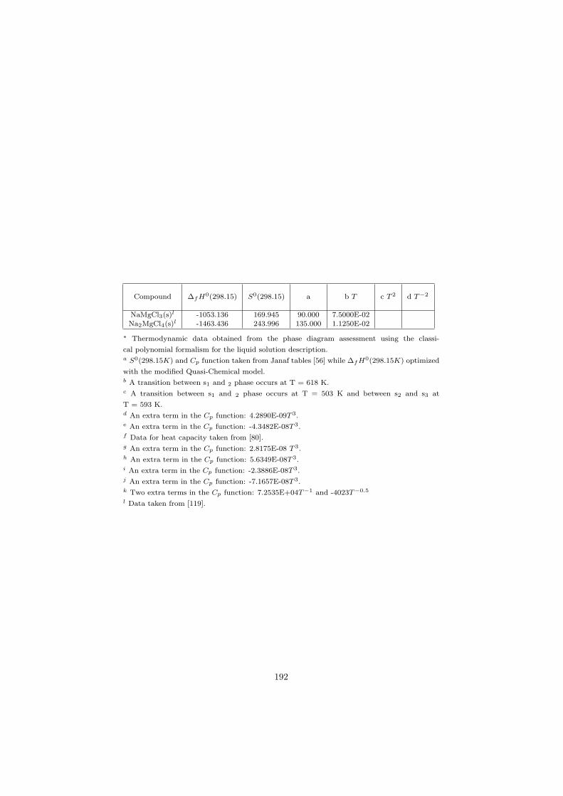
Compound ∆f H0(298.15) S0(298.15) a b T c T 2 d T−2

NaMgCl3(s)l -1053.136 169.945 90.000 7.5000E-02Na2MgCl4(s)l -1463.436 243.996 135.000 1.1250E-02

∗ Thermodynamic data obtained from the phase diagram assessment using the classi-

cal polynomial formalism for the liquid solution description.a S0(298.15K) and Cp function taken from Janaf tables [56] while ∆f H0(298.15K) optimized

with the modified Quasi-Chemical model.b A transition between s1 and 2 phase occurs at T = 618 K.c A transition between s1 and 2 phase occurs at T = 503 K and between s2 and s3 at

T = 593 K.d An extra term in the Cp function: 4.2890E-09T 3.e An extra term in the Cp function: -4.3482E-08T 3.f Data for heat capacity taken from [80].g An extra term in the Cp function: 2.8175E-08 T 3.h An extra term in the Cp function: 5.6349E-08T 3.i An extra term in the Cp function: -2.3886E-08T 3.j An extra term in the Cp function: -7.1657E-08T 3.k Two extra terms in the Cp function: 7.2535E+04T−1 and -4023T−0.5

l Data taken from [119].

192

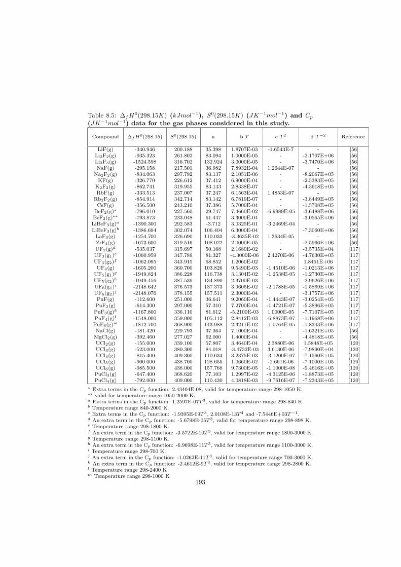
Table 8.5: ∆fH0(298.15K) (kJmol−1), S0(298.15K) (JK−1mol−1) and Cp

(JK−1mol−1) data for the gas phases considered in this study.

Compound ∆f H0(298.15) S0(298.15) a b T c T 2 d T−2 Reference

LiF(g) -340.946 200.188 35.398 1.8707E-03 -1.6543E-7 - [56]Li2F2(g) -935.323 261.802 83.094 1.0000E-05 - -2.1707E+06 [56]Li3F3(g) -1524.598 316.702 132.924 3.0000E-05 - -3.7470E+06 [56]NaF(g) -295.158 217.501 36.982 7.8932E-04 1.2644E-07 - [56]

Na2F2(g) -834.063 297.792 83.137 2.1051E-06 - -8.2067E+05 [56]KF(g) -326.770 226.612 37.412 6.9000E-04 - -2.5383E+05 [56]

K2F2(g) -862.741 319.955 83.143 2.8338E-07 - -4.3618E+05 [56]RbF(g) -333.513 237.007 37.247 6.1563E-04 1.4853E-07 - [56]

Rb2F2(g) -854.914 342.714 83.142 6.7819E-07 - -3.8449E+05 [56]CsF(g) -356.500 243.210 37.386 5.7000E-04 - -1.5708E+05 [56]

BeF2(g)∗ -796.010 227.560 29.747 7.4660E-02 -6.9989E-05 -3.6488E+06 [56]BeF2(g)∗∗ -793.873 233.048 61.447 3.3000E-04 - -3.0565E+06 [56]LiBeF3(g)a -1390.300 292.583 -3.712 3.0325E-01 -3.2469E-04 - [56]LiBeF3(g)b -1386.694 302.074 106.404 6.3000E-04 -7.3060E+06 [56]

LaF3(g) -1254.700 326.690 110.033 -3.3635E-02 1.3634E-05 - [56]ZrF4(g) -1673.600 319.516 108.022 2.0000E-05 - -2.5966E+06 [56]UF2(g)d -535.037 315.697 50.168 2.1680E-02 - -3.5735E+04 [117]UF3(g1)e -1060.959 347.789 81.327 -4.3000E-06 2.4270E-06 -4.7630E+05 [117]UF3(g2)f -1062.095 343.915 68.852 1.2060E-02 - 1.8451E+06 [117]UF4(g) -1605.200 360.700 103.826 9.5490E-03 -1.4510E-06 -1.0213E+06 [117]

UF5(g1)g -1949.824 386.228 116.738 3.1304E-02 -1.2538E-05 -1.2730E+06 [117]UF5(g2)h -1949.456 387.539 134.890 2.3700E-03 - -2.9626E+06 [117]UF6(g1)i -2148.642 376.573 137.373 3.9605E-02 -2.1788E-05 -1.5869E+06 [117]UF6(g2)j -2148.076 378.155 157.511 2.3000E-04 - -3.1757E+06 [117]PuF(g) -112.600 251.000 36.641 9.2060E-04 -1.4443E-07 -3.0254E+05 [117]PuF2(g) -614.300 297.000 57.310 7.2700E-04 -1.4721E-07 -5.3896E+05 [117]PuF3(g)k -1167.800 336.110 81.612 -5.2100E-03 1.0000E-05 -7.7107E+05 [117]PuF4(g)l -1548.000 359.000 105.112 2.8412E-03 -6.8873E-07 -1.1968E+06 [117]PuF6(g)m -1812.700 368.900 143.988 2.3211E-02 -1.0764E-05 -1.8343E+06 [117]NaCl(g) -181.420 229.793 37.364 7.1000E-04 - -1.6321E+05 [56]MgCl2(g) -392.460 277.027 62.000 1.4000E-04 - -4.4818E+05 [56]UCl2(g) -155.000 339.100 57.807 3.4640E-04 2.3880E-06 1.5848E+05 [120]UCl3(g) -523.000 380.300 84.018 -3.4732E-03 3.6130E-06 -7.9890E+04 [120]UCl4(g) -815.400 409.300 110.634 3.2375E-03 -3.1200E-07 -7.1560E+05 [120]UCl5(g) -900.000 438.700 128.655 1.0660E-02 -2.661E-06 -7.1000E+05 [120]UCl6(g) -985.500 438.000 157.768 9.7300E-05 -1.1000E-08 -9.4616E+05 [120]PuCl3(g) -647.400 368.620 77.103 1.2997E-02 -4.3125E-06 -1.8873E+05 [120]PuCl4(g) -792.000 409.000 110.430 4.0818E-03 -9.7616E-07 -7.2343E+05 [120]

∗ Extra terms in the Cp function: 2.43404E-08, valid for temperature range 298-1050 K.∗∗ valid for temperature range 1050-2000 K.a Extra terms in the Cp function: 1.2597E-07T 3, valid for temperature range 298-840 K.b Temperature range 840-2000 K.c Extra terms in the Cp function: -1.9395E-09T 3, 2.0108E-13T 4 and -7.5446E+03T−1.d An extra term in the Cp function: -5.6798E-05T 3, valid for temperature range 298-898 K.e Temperature range 298-1800 K.f An extra term in the Cp function: -3.5722E-10T 3, valid for temperature range 1800-3000 K.g Temperature range 298-1100 K.h An extra term in the Cp function: -6.9698E-11T 3, valid for temperature range 1100-3000 K.i Temperature range 298-700 K.j An extra term in the Cp function: -1.0262E-11T 3, valid for temperature range 700-3000 K.k An extra term in the Cp function: -2.4612E-9T 3, valid for temperature range 298-2800 K.l Temperature range 298-2400 Km Temperature range 298-1000 K

193

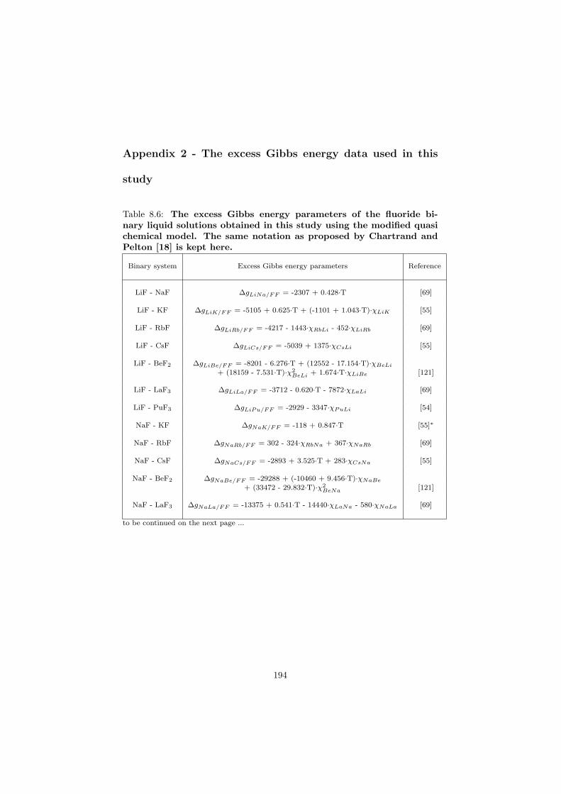
Appendix 2 - The excess Gibbs energy data used in this

study

Table 8.6: The excess Gibbs energy parameters of the fluoride bi-nary liquid solutions obtained in this study using the modified quasichemical model. The same notation as proposed by Chartrand andPelton [18] is kept here.

Binary system Excess Gibbs energy parameters Reference

LiF - NaF ∆gLiNa/FF = -2307 + 0.428·T [69]

LiF - KF ∆gLiK/FF = -5105 + 0.625·T + (-1101 + 1.043·T)·χLiK [55]

LiF - RbF ∆gLiRb/FF = -4217 - 1443·χRbLi - 452·χLiRb [69]

LiF - CsF ∆gLiCs/FF = -5039 + 1375·χCsLi [55]

LiF - BeF2 ∆gLiBe/FF = -8201 - 6.276·T + (12552 - 17.154·T)·χBeLi

+ (18159 - 7.531·T)·χ2BeLi + 1.674·T·χLiBe [121]

LiF - LaF3 ∆gLiLa/FF = -3712 - 0.620·T - 7872·χLaLi [69]

LiF - PuF3 ∆gLiPu/FF = -2929 - 3347·χPuLi [54]

NaF - KF ∆gNaK/FF = -118 + 0.847·T [55]∗

NaF - RbF ∆gNaRb/FF = 302 - 324·χRbNa + 367·χNaRb [69]

NaF - CsF ∆gNaCs/FF = -2893 + 3.525·T + 283·χCsNa [55]

NaF - BeF2 ∆gNaBe/FF = -29288 + (-10460 + 9.456·T)·χNaBe

+ (33472 - 29.832·T)·χ2BeNa [121]

NaF - LaF3 ∆gNaLa/FF = -13375 + 0.541·T - 14440·χLaNa - 580·χNaLa [69]

to be continued on the next page ...

194

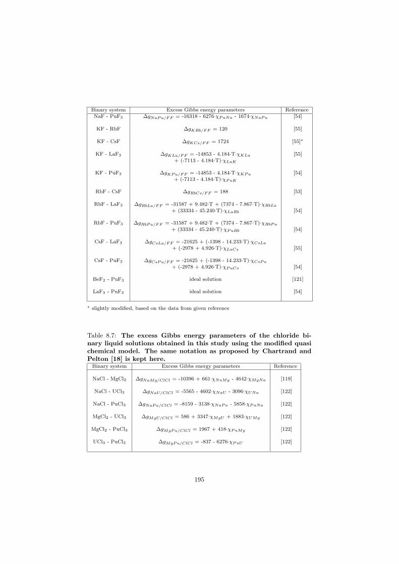
Binary system Excess Gibbs energy parameters ReferenceNaF - PuF3 ∆gNaPu/FF = -16318 - 6276·χPuNa - 1674·χNaPu [54]

KF - RbF ∆gKRb/FF = 120 [55]

KF - CsF ∆gKCs/FF = 1724 [55]∗

KF - LaF3 ∆gKLa/FF = -14853 - 4.184·T·χKLa [55]+ (-7113 - 4.184·T)·χLaK

KF - PuF3 ∆gKPu/FF = -14853 - 4.184·T·χKPu [54]+ (-7113 - 4.184·T)·χPuK

RbF - CsF ∆gRbCs/FF = 188 [53]

RbF - LaF3 ∆gRbLa/FF = -31587 + 9.482·T + (7374 - 7.867·T)·χRbLa

+ (33334 - 45.240·T)·χLaRb [54]

RbF - PuF3 ∆gRbPu/FF = -31587 + 9.482·T + (7374 - 7.867·T)·χRbPu

+ (33334 - 45.240·T)·χPuRb [54]

CsF - LaF3 ∆gCsLa/FF = -21625 + (-1398 - 14.233·T)·χCsLa

+ (-2978 + 4.926·T)·χLaCs [55]

CsF - PuF3 ∆gCsPu/FF = -21625 + (-1398 - 14.233·T)·χCsPu

+ (-2978 + 4.926·T)·χPuCs [54]

BeF2 - PuF3 ideal solution [121]

LaF3 - PuF3 ideal solution [54]

∗ slightly modified, based on the data from given reference

Table 8.7: The excess Gibbs energy parameters of the chloride bi-nary liquid solutions obtained in this study using the modified quasichemical model. The same notation as proposed by Chartrand andPelton [18] is kept here.

Binary system Excess Gibbs energy parameters Reference

NaCl - MgCl2 ∆gNaMg/ClCl = -10396 + 661·χNaMg - 4642·χMgNa [119]

NaCl - UCl3 ∆gNaU/ClCl = -5565 - 4602·χNaU - 3096·χUNa [122]

NaCl - PuCl3 ∆gNaPu/ClCl = -8159 - 3138·χNaPu - 5858·χPuNa [122]

MgCl2 - UCl3 ∆gMgU/ClCl = 586 + 3347·χMgU + 1883·χUMg [122]

MgCl2 - PuCl3 ∆gMgPu/ClCl = 1967 + 418·χPuMg [122]

UCl3 - PuCl3 ∆gMgPu/ClCl = -837 - 6276·χPuU [122]

195

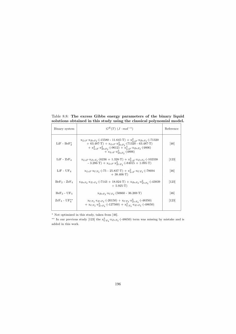
Table 8.8: The excess Gibbs energy parameters of the binary liquidsolutions obtained in this study using the classical polynomial model.

Binary system GE(T ) (J ·mol−1) Reference

xLiF ·xBeF2·(-15580 - 11.645·T) + x2

LiF ·xBeF2·(-71320

LiF - BeF∗2 + 63.487·T) + xLiF ·x2BeF2

·(71320 - 63.487·T) [46]

+ x2LiF ·x

2BeF2

·(-9612) + x3LiF ·xBeF2

·(4806)

+ xLiF ·x3BeF2

·(4806)

LiF - ZrF4 xLiF ·xZrF4·(6236 + 1.328·T) + x2

LiF ·xZrF4·(-102338 [123]

- 3.286·T) + xLiF ·x2ZrF4

·(-84015 + 1.095·T)

LiF - UF4 xLiF ·xUF4·(-75 - 25.837·T) + x2

LiF ·xUF4·(-78694 [46]

+ 38.406·T)

BeF2 - ZrF4 xBeF2·xZrF4

·(-7143 + 18.024·T) + xBeF2·x2

ZrF4·(-43839 [123]

+ 5.925·T)

BeF2 - UF4 xBeF2·xUF4

·(50660 - 36.269·T) [46]

ZrF4 - UF∗∗4 xUF4·xZrF4

·(-20150) + xUF4·x2

ZrF4·(-48350) [123]

+ xUF4·x3

ZrF4·(-127500) + x3

UF4·xZrF4

·(-48650)

∗ Not optimized in this study, taken from [46].∗∗ In our previous study [123] the x3

UF4·xZrF4

·(-48650) term was missing by mistake and is

added in this work.

196

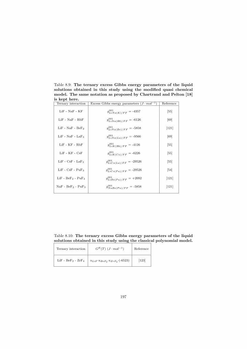
Table 8.9: The ternary excess Gibbs energy parameters of the liquidsolutions obtained in this study using the modified quasi chemicalmodel. The same notation as proposed by Chartrand and Pelton [18]is kept here.

Ternary interaction Excess Gibbs energy parameters (J ·mol−1) Reference

LiF - NaF - KF g001LiNa(K)/FF

= -4357 [55]

LiF - NaF - RbF g001LiNa(Rb)/FF

= -6126 [69]

LiF - NaF - BeF2 g001LiNa(Be)/FF

= -5858 [121]

LiF - NaF - LaF3 g001LiNa(La)/FF

= -9566 [69]

LiF - KF - RbF g001LiK(Rb)/FF

= -4126 [55]

LiF - KF - CsF g001LiK(Cs)/FF

= -6226 [55]

LiF - CsF - LaF3 g001LiCs(La)/FF

= -29526 [55]

LiF - CsF - PuF3 g001LiCs(Pu)/FF

= -29526 [54]

LiF - BeF2 - PuF3 g001LiBe(Pu)/FF

= +2092 [121]

NaF - BeF2 - PuF3 g001NaBe(Pu)/FF

= -5858 [121]

Table 8.10: The ternary excess Gibbs energy parameters of the liquidsolutions obtained in this study using the classical polynomial model.

Ternary interaction GE(T ) (J ·mol−1) Reference

LiF - BeF2 - ZrF4 xLiF ·xBeF2·xZrF4

·(-6523) [123]

197

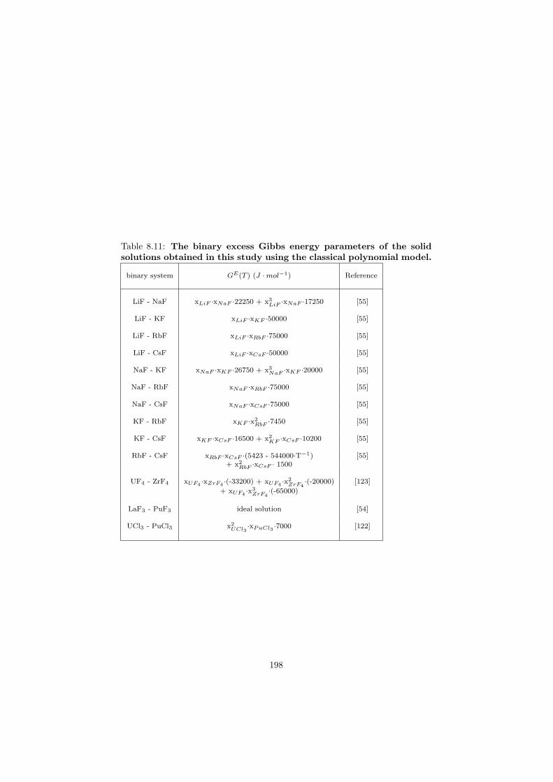
Table 8.11: The binary excess Gibbs energy parameters of the solidsolutions obtained in this study using the classical polynomial model.

binary system GE(T ) (J ·mol−1) Reference

LiF - NaF xLiF ·xNaF ·22250 + x3LiF ·xNaF ·17250 [55]

LiF - KF xLiF ·xKF ·50000 [55]

LiF - RbF xLiF ·xRbF ·75000 [55]

LiF - CsF xLiF ·xCsF ·50000 [55]

NaF - KF xNaF ·xKF ·26750 + x3NaF ·xKF ·20000 [55]

NaF - RbF xNaF ·xRbF ·75000 [55]

NaF - CsF xNaF ·xCsF ·75000 [55]

KF - RbF xKF ·x2RbF ·7450 [55]

KF - CsF xKF ·xCsF ·16500 + x2KF ·xCsF ·10200 [55]

RbF - CsF xRbF ·xCsF ·(5423 - 544000·T−1) [55]+ x2

RbF ·xCsF · 1500

UF4 - ZrF4 xUF4·xZrF4

·(-33200) + xUF4·x2

ZrF4·(-20000) [123]

+ xUF4·x3

ZrF4·(-65000)

LaF3 - PuF3 ideal solution [54]

UCl3 - PuCl3 x2UCl3

·xPuCl3 ·7000 [122]

198

Bibliography

[1] P. Pickard, Sulphur-Iodine Thermochemical Cycle, DOE Hydrogen Pro-gram Review, 2005 .

[2] H. G. MacPherson, Nucl. Sci. Eng. 90 (1985) 374.

[3] W. R. Grimes, D. R. Cuneo, Reactor Handbook, Vol. I, Materials, Inter-science Publishes Inc, New York, 1960, Ch. 17, p. 425.

[4] W. R. Grimes, Nucl. Appl. Tech. 8 (1970) 37.

[5] P. N. Haubenreich, J. R. Engel, Nucl. Appl. Technol. 8 (1970) 118–133.

[6] R. C. Robertson, Technical Report ORNL-4541, Tech. rep. (1971).

[7] A. L. Zherebtsov, V. V. Ignatiev, Experimental Mock-Up of Accelerator-Based Facility for Transmutation of Radioactive Waste and Conversionof Military Plutonium, Tech. rep., Nr. 1606 Annual Report (2006).

[8] L. Mathieu, Exploration du champ des parametres et des contraintesdefinissant le thorium molten salt reactor, PhD thesis, France (in French)(2005) .

[9] L. Mathieu, et al., Proposition for a very simle thorium molten salt reactor,Global Conference, Tsukuba, Japan (2005) .

[10] L. Mathieu, et al., Prog. in Nucl. En. 48 (2006) 664–679.

[11] E. Merle-Lucotte, et al., Fast thorium molten salt reactors started withplutonium, Proceedings of the International Congress on Advances in Nu-clear Power Plants (ICAPP), Reno, USA (2006) .

[12] E. Merle-Lucotte, D. Heuer, C. L. Brun, M. Allibert, V. Ghetta, TheTMSR as Actinide Burner and Thorium Breeder, Note LPSC 07-37 (2007).

[13] A. Mourogov, P. M. Bokov, Energy Conversion and Management 47 (2006)2761.

199

[14] C. W. Bale, et al., FactSage Software v. 5.5.

[15] J. L. Holm, Acta Chem. Scand. 19 (1965) 638.

[16] A. D. Pelton, P. Chartrand, G. Eriksson, Metall. Trans. 32A (2001) 1409–1416.

[17] P. Chartrand, A. D. Pelton, Metall. Trans. 32A (2001) 1397–1407.

[18] P. Chartrand, A. D. Pelton, Metall. Trans. 32A (2001) 1385.

[19] R. W. Cahn, P. Haasen, Physical Metallurgy, Vol. Volume 1, ElsevierScience, Amsterdam, 1996, Ch. Phase diagrams, p. 509.

[20] A. T. Dinsdale, Calphad 15 (1991) 317–425.

[21] NIST, Standard reference material No. 720.

[22] D. Sedmidubsky, DSCEval-software for DSC-data evaluation, Institute ofChemical Technology, Prague, Czech Republic, 2000.

[23] R. Burriel, M. W. K. To, H. Zainel, E. F. W. Jr., E. H. P. Cordfunke,R. P. Muis, G. Wijbenga, J. Chem. Thermodynamics 20 (1988) 815–823.

[24] O. Benes, R. Jardin, R. J. M. Konings, E. Colineau, F. Wastin, N. Mag-nani, The high-temperature heat capacity of ThPd3 and UPd3, J. Chem.Thermodyn. submitted.

[25] H. C. Walker, K. A. McEwen, D. F. McMorrow, S. B. Wilkins, F. Wastin,E. Colineau, D. Fort, Phys. Rev. Lett. 10.1103/PhysRevLett.97.137203.

[26] Y. Arita, N. Sasajima, T. Matsui, J. Nucl. Mat. 247 (1997) 232–234.

[27] W. J. L. Buyers, T. M. Holden, Handbook on the Physics and Chemistryof the Actinides, Vol. 2, Elsevier Science, Amsterdam, 1985, p. 289.

[28] Y. Tokiwa, et al., Journal of the Physical Society of Japan 70 (2001)1731–1743.

[29] K. A. McEwen, H. C. Walker, M. D. Le, D. F. McMorrow, E. Colineau,F. Wastin, S. B. Wilkins, J.-G. Park, R. I. Bewley, D. Fort, J. Magn.Magn. Mat. 310 (2007) 718–722.

[30] R. J. M. Konings, J. P. M. van der Meer, E. Walle, Chemical aspects ofMolten Salt Reactor Fuel, Tech. rep., ITU-TN 2005/25 (2005).

[31] P. D. Desai, Int. J. Therm. 8 (1987) 763–780.

[32] W. H. Madgin, H. V. A. Briscoe, J. Chem. Soc. 123 (1923) 2914–2916.

[33] A. G. Bergmann, S. I. Berul, Anal. Inst. Obshch. Neorg. Khim. Akad.Nauk SSSR 21 (1952) 178–183.

200

[34] S. I. Berul, A. G. Bergmann, Anal. Inst. Obshch. Neorg. Khim. Akad.Nauk SSSR 25 (1954) 218–235.

[35] A. Kofler, Montash. Chem. 86 (1955) 643–652.

[36] A. N. Kirgintsev, V. I. Kosyakov, Izv. Akad. Nauk SSSR, Ser Khim. 10(1968) 2208–2213.

[37] M. P. Susarov, A. I. Efimov, L. S. Timoshenko, Russ. J. Phys. Chem. 43(1969) 795–799.

[38] W. Klement, J. Inorg. Nucl. Chem. 36 (1974) 1916–1918.

[39] C. M. Kramer, C. J. Wilson, Thermochim. Acta 42 (1980) 253–264.

[40] D. J. Rogers, G. J. Janz, J. Chem. Eng. Data 27 (1982) 424–428.

[41] O. Greis, K. M. Bahamdan, B. M. Uwais, Thermochim. Acta 86 (1985)343–350.

[42] X. Zhang, J. Tian, K. Xu, Y. Gao, J. Ph. Equilib. 24 (2003) 441–446.

[43] T. Jriri, J. Rogez, J. C. Mathieu, I. Ansara, J. Phas. Equilib. 20 (1999)515–525.

[44] T. Jriri, J. Rogez, C. Bergman, J. C. Mathieu, Thermochimica Acta 266(1995) 147–161.

[45] R. G. Samuseva, V. E. Plyushchev, Russ. J. Inorg. Chem. 10 (1965) 688.

[46] J. van der Meer, R. J. M. Konings, H. A. J. Oonk, J. Nucl. Mat. 357(2006) 48–57.

[47] S. J. Clark, M. D. Segall, C. J. Pickard, P. J. Hasnip, M. J. Probert,K. Refson, M. C. Payne, Zeitschrift fur Krystallographie 220 (2005) 567–570.

[48] Material Studio v. 4.3.0.0, Accelrys Software Inc.

[49] J. C. Mathieu, F. Durand, E. Bonnier, J. Chim. Phys. 62 (1965) 1289.

[50] J. C. Mathieu, F. Durand, E. Bonnier, J. Chim. Phys. 62 (1965) 1297.

[51] W. L. Bragg, E. J. Williams, Proc. Roy. Soc. A145 (1934) 699.

[52] E. A. Guggenheim, Mixtures, OXFORD Clarendon Press, 1952.

[53] O. Benes, P. Zeller, M. Salanne, R. J. M. Konings, Ab initio and moleculardynamic study of the (Rb,Cs)F solid and liquid solutions, J. Chem. Phys.,submitted, (2008) .

[54] O. Benes, R. J. M. Konings, J. Nucl. Mat. 377 (3) (2008) 449–457.

201

[55] O. Benes, R. J. M. Konings, Computer Coupling of Phase Diagrams andThermochemistry 32 (2008) 121–128.

[56] M. W. Chase Jr.(ed.), NIST-JANAF Thermochemical Tables Fourth Edi-tion, J. Phys. Chem. Ref. Data, Monograph 9 (1998) .

[57] K. C. Hong, O. J. Kleppa, J. Phys. Chem. 83 (1979) 2589.

[58] J. L. Holm, O. J. Kleppa, J. Chem. Phys. 49 (1968) 2425.

[59] A. C. Macleod, J. Cleland, J. Chem. Thermodynamics 7 (1975) 103.

[60] R. E. Thoma, Advances in Molten Salt Chemistry, Vol. 3, Plenum Press,1975, Ch. 6, p. 275.

[61] A. G. Bergmann, S. P. Pavlenko, C. R. Acad. Sci. URSS 30 (1941) 812.

[62] N. N. Volkov, L. A. Dubinskaya, Izv. Fiz.-Khim. Nauchno.-Issled. Inst.Irkutsk. Gos. Univ. 2 (1953) 45.

[63] A. G. Bergmann, N. A. Bychkova-Schul’ga, Russ. J. Inorg. Chem. 2 (1957)276.

[64] A. G. Bergmann, V. P. Goryacheva, Russ. J. Inorg. Chem. 7 (1962) 1359.

[65] E. Aukrust, B. Bjorge, H. Flood, T. Forland, Ann. N. Y. Acad. Sci. 79(1960) 830.

[66] G. A. Bukhalova, Z. N. Topshinoeva, V. G. Akhtyrskii, Zh. Neorg. Khim.19 (1974) 235.

[67] J. Sangster, A. D. Pelton, J. Phys. Chem. Ref. Data 16 (1987) 509.

[68] K. C. Hong, O. J. Kleppa, J. Chem. Thermodynamics 8 (1976) 31.

[69] O. Benes, J. P. M. van der Meer, R. J. M. Konings, Computer Couplingof Phase Diagrams and Thermochemistry 31 (2007) 209–216.

[70] C. J. Barton, V. S. Coleman, L. M. Bratcher, R. R. Grimes, Oak RidgeNational Laboratory (unpublished).

[71] G. A. Bukhalova, D. V. Sementsova, Russ. J. Inorg. Chem. 10 (1965) 1024.

[72] J. L. Holm, O. J. Kleppa, Inorg. Chem. 8 (1969) 207.

[73] D. M. Roy, R. Roy, E. F. Osborn, J. Am. Ceram. Soc. 37 (1954) 300.

[74] R. E. Thoma, H. Insley, H. A. Friedman, G. M. Hebert, J. Nucl. Mater.27 (1968) 166.

[75] K. A. Romberger, J. Braunstein, R. E. Thoma, J. Phys. Chem. 76 (1972)1154.

202

[76] B. F. Hitch, C. F. Baes Jr., Inorg. Chem. 8 (1969) 201.

[77] J. van der Meer, R. J. M. Konings, M. H. G. Jacobs, H. A. J. Oonk, J.Nucl. Mat. 344 (2005) 94–99.

[78] M. A. Greenbaum, J. N. Foster, M. L. Arin, M. Farber, J. Phys. Chem.67 (1963) 36.

[79] J. P. M. van der Meer, R. J. M. Konings, K. Hack, H. A. J. Oonk, Chem.Mater. 18 (2006) 510–517.

[80] F. Abdoun, M. Gaune-Escard, G. Hatem, J. Phase Equil. 18 (1997) 6.

[81] G. A. Bukhalova, E. P. Babaeva, Russ. J. Inorg. Chem. 10 (1965) 1026.

[82] L. A. Khripin, Izv. Sibir. Otdel. Akad. Nauk SSSR, Ser Khim. Nauk 7(1963) 107.

[83] R. E. Thoma, G. D. Brunton, R. A. Penneman, T. K. Keenan, Inorg.Chem. 9 (1970) 1096.

[84] A. I. Agulyanskii, V. Bessonova, Russ. J. Inorg. Chem. 27 (1982) 579.

[85] R. E. Thoma, H. Insley, H. A. Friedman, G. M. Hebert, J. Chem. Eng.Data 10 (1965) 219.

[86] C. J. Barton, R. A. Strehlow, J. Inorg. Nucl. Chem. 18 (1961) 143–149.

[87] D. L. Deadmore, J. S. Machin, J. Phys. Chem. 64 (1960) 824.

[88] R. G. Samuseva, V. E. Plyushchev, Russ. J. Inorg. Chem. 6 (1961) 1092.

[89] K. A. Sense, R. W. Stone, J. Phys. Chem. 62 (1958) 453–457.

[90] G. T. Fukuda, P. F. Peterson, D. R. Olander, J. M. Prausnitz, Fluid PhaseEquilibria 255 (2007) 1–10.

[91] C. J. Barton, J. D. Redman, R. A. Strehlow, J. Inorg. Nucl. Chem. 20(1961) 45–49.

[92] R. E. Thoma, Phase diagrams of nuclear reactor materials, ORNL Report2548.

[93] E. P. Dergunov, A. G. Bergman, Zh. Fiz. Khim. 22 (1948) 625.

[94] N. C. Tkachev, High Temperature and Material Science 35 (1996) 247.

[95] E. P. Dergunov, Dokl. Akad. Nauk SSSR 60 (1948) 1187.

[96] G. A. Bukhalova, E. P. Babaeva, T. M. Khliyan, Russ. J. Inorg. Chem.10 (1965) 1158.

[97] K. Tchi-Tsu, A. V. Novocelova, Zh. Neorg. Khim. 9 (1961) 2148.

203

[98] T. G. Filatova, B. S. Zakharova, L. P. Reshetrikova, A. W. Novoselova,Zh. Neorg. Khim. 25 (1980) 1427.

[99] P. P. Fedorov, Russ. J. Inorg. Chem. 44 (1999) 1703–1727.

[100] T. G. Filatova, P. P. Fedorov, Russ. J. Inorg. Chem. 45 (2000) 785–788.

[101] C. J. Barton, W. R. Grimes, H. Insley, R. E. Moore, R. Thoma, J. Phys.Chem. 62 (1958) 665.

[102] M. Taube, Fast reactors using molten chloride slats as fuel, in: Swissfederal institute for reactor research, Wurenlingen, Swiss, 1978.

[103] C. W. Bjorklund, J. G. Reavis, J. A. Leary, K. A. Walsh, J. Phys. Chem.63 (1959) 1774–1777.

[104] M. P. Morobei, V. N. Desyatnik, O. V. Skiba, N. M. Emel’yanov, Russ.J. Inorg. Chem. 18 (1973) 1628.

[105] V. N. Desyatnik, Y. A. Izmodenov, Y. T. Mel’nikov, I. F. Nichkov, S. P.Raspopin, Atomnaya Energiya 26 (1969) 549–550.

[106] K. W. R. Johnson, M. Kahn, J. A. Leary, J. Phys. Chem. 65 (1961) 1461–1462.

[107] O. Benes, R. J. M. Konings, Thermodynamic properties and phase di-agrams of fluoride salts for nuclear applications, J. Fluorine Chem., inpress, (2008) doi:10.1016/j.jfluchem.2008.07.014.

[108] J. Sangster, A. D. Pelton, J. Phase Equil. 12 (1991) 511.

[109] A. G. Bergmann, E. P. Dergunov, Dokl. Ac. Sc. URSS 31 (1941) 753.

[110] R. E. Moore, C. J. Barton, W. R. Grimes, R. E. Meadows, L. M. Bratcher,G. D. White, T. N. McVay, Tech. Rep. ORNL, unpublished work (1951-1958).

[111] C. J. Barton, J. Phys. Chem. 64 (1959) 306.

[112] J. C. Mailen, F. J. Smith, L. M. Ferris, J. Chem. Eng. Data 16 (1971)68–74.

[113] International Scientific Technical Centre, Moscow, Tech. rep., ISTCProject #1606 Final Report (July 2004).

[114] C. Forsberg, Molten salt reactors (msrs), proceedings of The Americas Nu-clear Energy Symposium American Nuclear Society (ANES 2002), Miami,Florida.

[115] W. R. Grimes, Nucl. Appl. Tech. 8 (1969) 137.

204

[116] I. Barin, O. Knacke, O. Kubaschewski, Thermochemical Properties ofInorganic Substances, Springer-Verlag, Berlin (1977) .

[117] R. J. M. Konings, L. R. Morss, J. Fuger, The Chemistry of the Actinideand Transactinide Elements, Vol. 4, Springer, Dordrecht, The Nether-lands, 2006, Ch. 19.

[118] J. Serp, R. J. M. Konings, R. Malmbeck, J. Rebizant, C. Scheppler, J.-P.Glatz, J. Electroanal. Chem. 561 (2003) 143–148.

[119] P. Chartrand, A. D. Pelton, Metall. Trans. 32A (2001) 1361.

[120] R. Guillaumont, T. Fanghanel, V. Neck, J. Fuger, D. A. Palmer, I. Gren-the, M. H. Rand, Update on the Chemical Thermodynamics of Uranium,Neptunium, Plutonium, Americium and Technetium, Vol. Chemical Ther-modynamics, Vol. 5, OECD Nuclear Energy Agency, 2003.

[121] O. Benes, R. J. M. Konings, Thermodynamic evaluation of the LiF-NaF-BeF2-PuF3 system; an actinide burner fuel, J. Chem. Thermodyn., sub-mitted, (2008) .

[122] O. Benes, R. J. M. Konings, J. Nucl. Mat. 375 (2008) 202–208.

[123] O. Benes, R. J. M. Konings, J. Alloys Compd. 452 (2008) 110–115.

205

Distribution List: Mr. Fanghänel ITU 1x Mr. Wastin ITU 1x Mr. Konings ITU 1x Mr. Sedmidubsky ITU 1x Mr. Manara ITU 1x Mr. Beilmann ITU 1x Mr. Soucek ITU 1x Mr. Vlahovic ITU 1x Mrs. Weber ITU 3x JRC-ITU-TN-2008/40 European Commission– Joint Research Centre – Institute for Transuranium Elements Title: THERMODYNAMICS OF MOLTEN SALTS FOR NUCLEAR APPLICATIONS Author: O. Beneš 2008 – 214 pp. – 21.0 x 29.7 cm

The mission of the JRC is to provide customer-driven scientific and technical supportfor the conception, development, implementation and monitoring of EU policies. As a service of the European Commission, the JRC functions as a reference centre of science and technology for the Union. Close to the policy-making process, it serves the common interest of the Member States, while being independent of special interests, whether private or national.