EUR 25259 EN - 2012

ASTRA Plus User Manual

Description of how to use the modules for Fault Tree Analysis andConcurrent Importance and Sensitivity Analysis

Vaidas Matuzas and Sergio Contini

The mission of the JRC-IPSC is to provide research results and to support EU policy-makers in their effort towards global security and towards protection of European citizens from accidents, deliberate attacks, fraud and illegal actions against EU policies. European Commission Joint Research Centre Institute for the Protection and Security of the Citizen Contact information Address: Sergio Contini E-mail: Sergio.contini@jrc.ec.europa.eu Tel.: +39 0332 789217 Fax: +39 0331 785145 http://ipsc.jrc.ec.europa.eu/ http://www.jrc.ec.europa.eu/ Legal Notice Neither the European Commission nor any person acting on behalf of the Commission is responsible for the use which might be made of this publication.

Europe Direct is a service to help you find answers to your questions about the European Union

Freephone number (*):

00 800 6 7 8 9 10 11

(*) Certain mobile telephone operators do not allow access to 00 800 numbers or these calls may be billed.

A great deal of additional information on the European Union is available on the Internet. It can be accessed through the Europa server http://europa.eu/ JRC 69424 EUR 25259 ENISBN 978-92-79-23390-6 ISSN 1831-9424 doi:10.2788/17628 Luxembourg: Publications Office of the European Union, 2012 © European Union, 2012 Reproduction is authorised provided the source is acknowledged Printed in Italy

ABSTRACT This report describes the user interface and the main commands to perform system dependability analysis by means of ASTRA Plus. This package implements the analysis methods developed at the Institute for the Protection and Security of the Citizen from mid-2008. ASTRA Plus is composed of the Fault Tree Analysis (FTA) module and of the Concurrent Importance and Sensitivity Analysis (CISA) module. The FTA module contains three different methods for solving a fault tree; all are based on the state of the art approach of Binary Decision Diagrams (BDD). These three methods allow the user to analyse fault tree of increasing complexity (i.e. increasing number of basic events and gates). In particular the third method, which is based on functional decomposition, allows performing the analysis of fault trees of very high complexity. The CISA module is based on a new methodology for system design improvement. The key operation is the calculation of Global Importance Measures of basic events considering all system fault trees. This allows identifying the weakest part of the system with reference to all top-events. Then the on-line sensitivity analysis, allows the user to rapidly identify the set of suitable design improvements from which the best cost-effective one can be selected.

CONTENT TheASTRA Plus software ...................................................................................................4 General considerations ........................................................................................................8 Installing ASTRA Plus......................................................................................................11 ASTRA Plus .....................................................................................................................12

Software Interface .........................................................................................................12 Project Management......................................................................................................13

Create new project.....................................................................................................13 Opening existing project ...........................................................................................15

Working with fault trees................................................................................................16 Adding new fault tree ................................................................................................17 Deleting fault tree......................................................................................................18 Editing fault tree........................................................................................................19 Importing fault trees ..................................................................................................27 Exporting fault trees ..................................................................................................28

Analysing fault trees......................................................................................................28 BDD Analysis............................................................................................................29 TZBDD Analysis.......................................................................................................31 Decomposition analysis.............................................................................................31 Viewing analysis results............................................................................................33

House events..................................................................................................................38 Setting the House event state directly .......................................................................38 Setting the House event state through boundary conditions .....................................38

Boundary Condition Sets...............................................................................................38 ASTRA Plus – PRA Settings ........................................................................................41

ASTRA Plus – CISA.........................................................................................................42 Software Interface .........................................................................................................42 ASTRA Plus – CISA Project.........................................................................................43

Create new project.....................................................................................................43 Opening existing project ...........................................................................................45

Working with ASTRA Plus – CISA project .................................................................47 Adding new modification..........................................................................................47 Deleting modification................................................................................................53

Viewing CISA Analysis Results ...................................................................................53 Probabilistic results ...................................................................................................53 Importance analysis results .......................................................................................55 Summary of modifications ........................................................................................58 Ranking of modifications ..........................................................................................59

Managing CISA Project Data........................................................................................59 Modifying Probabilistic Goals ..................................................................................59 Modifying project data ..............................................................................................60 Viewing shared events...............................................................................................60

THE ASTRA PLUS SOFTWARE ASTRA Plus is the second generation of fault-tree analysis software developed by the European Commission, Joint Research Centre (JRC), at the Institute for the Protection and Security of the Citizen (IPSC), Ispra, Italy. It is fully based on Binary Decision Diagram (BDD), the state of the art approach. It was developed as an extended version of the JRC ASTRA 3.x software to cope with the analysis of fault trees of any complexity. The implemented analysis methods are the result of the authors’ research on complex systems dependability analysis. The new software comes with many improvements allowing the user to perform different tasks more easily and efficiently. ASTRA Plus consists of two tools:

• ASTRA Plus – FTA. This is the fault tree editing and analysis tool. It allows creating, managing and analysing fault trees of any complexity. It is used to prepare the input to the next tool.

• ASTRA Plus – CISA. This is the Concurrent Importance and Sensitivity Analysis tool which is based on a new methodology developed at the JRC-IPSC. It allows evaluating different design modifications and their effects on the system availability or safety.

ASTRA Plus – FTA implements the state of the art methods for fault tree analysis. The Binary Decision Diagrams (BDD) is the basic method of analysis, which was implemented in ASTRA 3.x. The BDD is presently by far the fastest method to analyse coherent and non-coherent fault trees. A BDD is a compact graph representation of Boolean functions. The main advantage of the BDD approach with respect to previous approaches is the possibility to obtain a compact graph embedding all system failure modes. On this graph system’s failure modes are mutually exclusive, a property that allows to perform the exact probabilistic quantification. Then, another graph can be derived embedding all Minimal Cut Sets (MCS), from which the Significant MCS (SMCS) can easily be extracted using the classical (probabilistic / logical) cut-off techniques. However, when the available working memory is not sufficient to store the BDD nodes, the method fails. This is due to the exponential increase in the number of nodes with the complexity of the fault tree. In these cases ASTRA Plus offers to the user the TZBDD module able to construct a smaller BDD, referred to as TZBDD (Truncated ZBDD) embedding only the SMCS. This is obtained by applying the probabilistic and/or logical cut-off techniques during the construction of the graph. Since the TZBDD contains only a small percentage of the MCS, it is not possible to know whether the probabilistic quantification underestimates or overestimates the Top event probability. Consequently, it is necessary to perform two or more runs with lower probabilistic cut-off thresholds until to the result shows at least an almost constant behaviour. In other words it is necessary to perform the analysis of the fault tree two or more times, with lower cut-off thresholds, until the difference between two runs can be considered negligible. In this case upper and lower bounds of the top-event unavailability can be calculated. With very complex fault trees, generally representing event tree sequences of nuclear safety models, it may happen that also the TZBDD method is not able to complete the analysis, i.e. it is not possible to reach the steady state condition of the top event unavailability function. In these cases ASTRA Plus offers the possibility to apply a third, and more complex, analysis method developed by the authors. This new method is based on the functional decomposition of the Boolean function representing the fault tree structure. More precisely, the complex fault tree is decomposed into a set of mutually exclusive simpler fault trees. The decomposition is repeatedly applied until the generated trees are sufficiently simple to be analysed with the available working memory.

Theoretically, this approach would allow performing the exact analysis of fault trees of any complexity, but the related computation times are generally too high to be practically useful. Therefore the decomposition has been combined with the cut-off technique to reduce the total computation time. This method - referred to as Decomposition plus Truncation (D+T) - provides upper and lower bounds of the Top-event probability. Experimental results showed that these bounds are generally very close to the exact value and that their difference depends on the dimension of the available working memory. Thanks to the mutual exclusivity of the generated simpler trees the probabilistic quantification, including the importance measures of basic events, can easily be performed by properly combining the results from the independent analysis of all simpler fault trees. With respect to ASTRA 3.x, ASTRA Plus adds new features, the most important of which are listed below:

• New interface including a new and more powerful graphical fault-tree editor; • Introduction of House events, allowing altering fault trees in an ease way; • Fault tree linking by using transfer gates; • Database support to store all project data; • Sharing (reuse) of different fault tree analysis objects (events, gates, boundary conditions, etc)

within the same project; • Two new BDD methods for fault-tree analysis, i.e. TZBDD and D+T; • Uncertainty analysis (propagation of data uncertainty from basic events to Top); • Possibility to analyse the same fault trees with different settings/analysis methods and to

maintain all results in the database; • New components’ importance measures based on failure frequency; • Sensitivity analysis concurrently performed on multiple fault trees;

A complex critical system may fail in different ways, some of which may entail unacceptable consequences to human beings and to the environment. Fault tree analysis is applied to model the failure logic of each of these states (Top events) to verify the adequacy of safety barriers in place. Fault tree analysis provides the failure probability / frequency of the top-event and several components importance measures. These results are then used, through the application of the Importance and Sensitivity Analysis (ISA), to improve plant safety by taking into account, if necessary and available, the design modifications costs. The current practice is that these fault-trees are analyzed independently, one at a time, starting for instance from the one with the most severe consequences. This approach, referred to as Sequential Importance and Sensitivity Analysis (SISA), has a number of disadvantages and limitations when the N Fault-trees are not independent (i.e. contain common basic events). In particular, the resulting design modification could not be the best cost-effective, since it depends on the sequence of examination of the Fault-trees. A possible way forward to overcome the limitations of the SISA approach is to apply the Concurrent Importance and Sensitivity Analysis (CISA) addressed to the unavailability analysis of the system. This approach was based on the calculation of components’ global importance index, i.e. importance referred to the system as a whole and not to a particular Top-event. A peculiar aspect is that CISA addresses also components with the lowest importance indexes, which are generally associated to “over-reliable” or “over-protected” system functions. Hence the final objective of this approach is to support the analyst in obtaining a uniformly protected system, by removing not only the “weak functions”, probable causes of system failure, but also uselessly “over-protected functions”, causes of major costs. Recently the CISA approach has been extended to cover also the unreliability analysis. In this manner it is possible to apply the method to the analysis of catastrophic events based on the unconditional failure frequency.

The present document describes the user interface of ASTRA Plus as well as the commands for data editing and analysis. It is subdivided into two parts, dedicated respectively to FTA and CISA tools. The theoretical basis and the main implemented algorithms are described in different reports and papers. In particular:

• The BDD logical and probabilistic analysis methods are described in [1]; the BDD is one of the three fault tree analysis methods implemented in ASTRA Plus which is common to ASTRA 3.x;

• A subset of fault trees used during the testing campaign of the BDD and TZBDD analysis methods are provided in [2].

• The TZBDD method is described in [3]; • The Decomposition and Truncation (D+T) method for the analysis of fault trees of any

complexity is provided in [4, 5, 6, 7]; • The basic theory of the Concurrent Importance and Sensitivity Analysis (CISA) method is

given in references [8, 9, 10,11]; • The Importance analysis is described in [12, 13];

General considerations on ASTRA Plus In order to better understand how ASTRA Plus works it is convenient to present some definitions of the objects used and their interdependencies. Fault-tree is a graphical representation of cause-consequence relationships between components’ failures and system failure described by the Top-event. The fault tree consists of gates and event. Fault-tree analysis is a deductive logical-probabilistic analysis technique that provides the Boolean representation of the cause-consequence relationships and the probability / failure frequency of the Top event. Gate represents logical (Boolean) operation applied on its descendents. Basic event is an event describing the state of a component (generally failure) not requiring further development. House event is an event, which is normally expected to occur (set to 1), or not (set to 0). Boundary condition set is a group (set) of boundary conditions. Boundary condition is a one of two marginal states of a basic event - working state and failed state. Analysis case is a set of data and assumptions for the analysis of a fault tree. In ASTRA Plus it is important to understand the relationships among the objects used in the project in order to make the modelling process easier. The main relationships are provided in Figure 1. In ASTRA Plus events, parameters and boundary conditions are defined as independent objects. This makes the construction and analysis of the fault trees very flexible because those elements can be reused many times within the same project. The central part of the analysis is the fault tree. It is done by using defined events and gates. Because events are defined independently from the fault tree – they can be shared, i.e. the same events can be used in different fault trees within the same project (as well as the same parameter can be shared by many events). An analysis case is defined as an independent object; this approach allows performing and keeping the results of the analysis of multiple fault trees using different settings and/or boundary condition sets. All data are stored into the database and “closed” in the ASTRA Plus-FTA project. This project represents the input of the CISA module for the system design improvement phase.

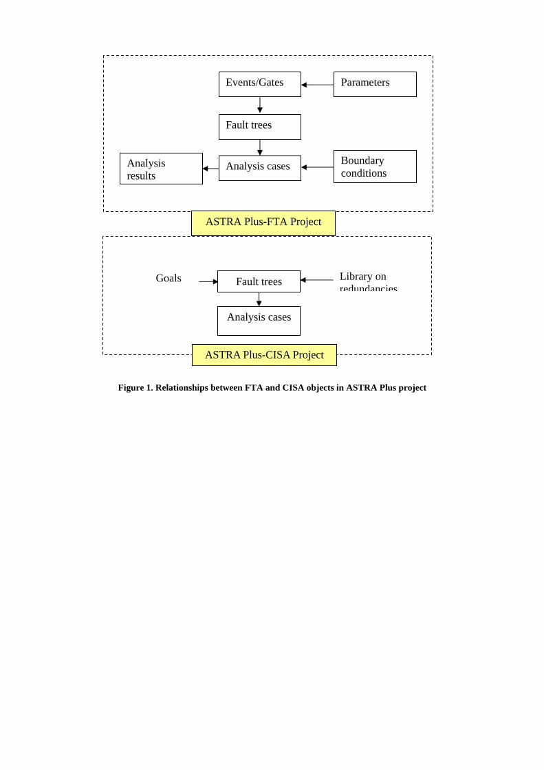
Figure 1. Relationships between FTA and CISA objects in ASTRA Plus project

Fault trees

Events/Gates

Boundary conditions Analysis cases

Parameters

Analysis results

ASTRA Plus-FTA Project

Fault trees Library on redundancies

Analysis cases

ASTRA Plus-CISA Project

Goals

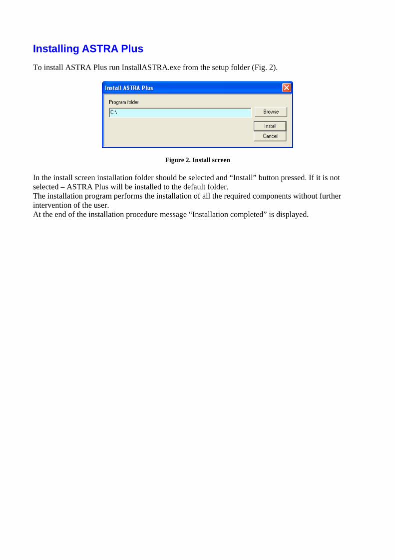
Installing ASTRA Plus To install ASTRA Plus run InstallASTRA.exe from the setup folder (Fig. 2).

Figure 2. Install screen In the install screen installation folder should be selected and “Install” button pressed. If it is not selected – ASTRA Plus will be installed to the default folder. The installation program performs the installation of all the required components without further intervention of the user. At the end of the installation procedure message “Installation completed” is displayed.

The FTA module of ASTRA Plus

Software Interface The ASTRA Plus graphical user interface has been designed to be simple and intuitive. There are two different interfaces:

• Welcome screen; • Working screen.

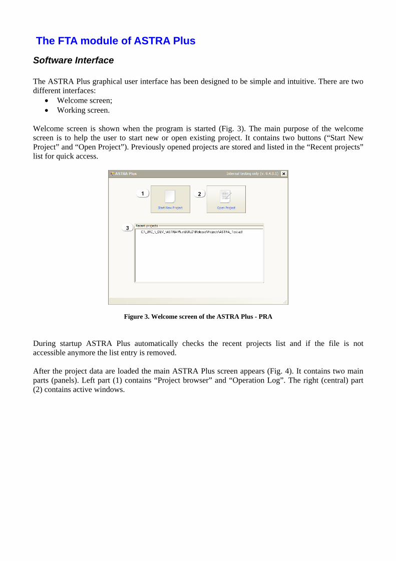
Welcome screen is shown when the program is started (Fig. 3). The main purpose of the welcome screen is to help the user to start new or open existing project. It contains two buttons (“Start New Project” and “Open Project”). Previously opened projects are stored and listed in the “Recent projects” list for quick access.

Figure 3. Welcome screen of the ASTRA Plus - PRA During startup ASTRA Plus automatically checks the recent projects list and if the file is not accessible anymore the list entry is removed. After the project data are loaded the main ASTRA Plus screen appears (Fig. 4). It contains two main parts (panels). Left part (1) contains “Project browser” and “Operation Log”. The right (central) part (2) contains active windows.

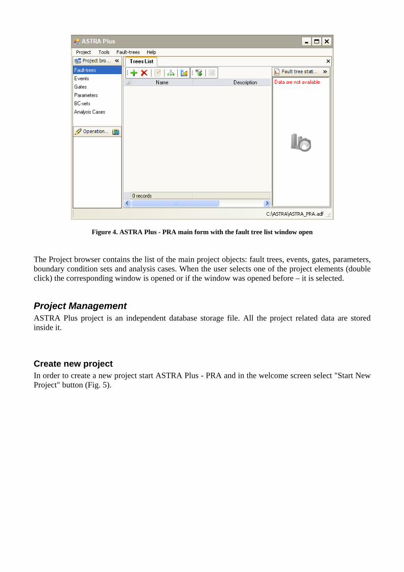
Figure 4. ASTRA Plus - PRA main form with the fault tree list window open The Project browser contains the list of the main project objects: fault trees, events, gates, parameters, boundary condition sets and analysis cases. When the user selects one of the project elements (double click) the corresponding window is opened or if the window was opened before – it is selected.

Project Management ASTRA Plus project is an independent database storage file. All the project related data are stored inside it.

Create new project In order to create a new project start ASTRA Plus - PRA and in the welcome screen select "Start New Project" button (Fig. 5).

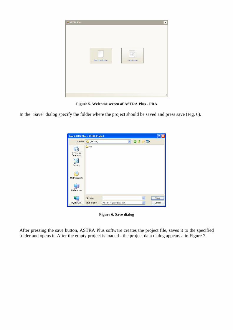
Figure 5. Welcome screen of ASTRA Plus - PRA In the "Save" dialog specify the folder where the project should be saved and press save (Fig. 6).

Figure 6. Save dialog After pressing the save button, ASTRA Plus software creates the project file, saves it to the specified folder and opens it. After the empty project is loaded - the project data dialog appears a in Figure 7.

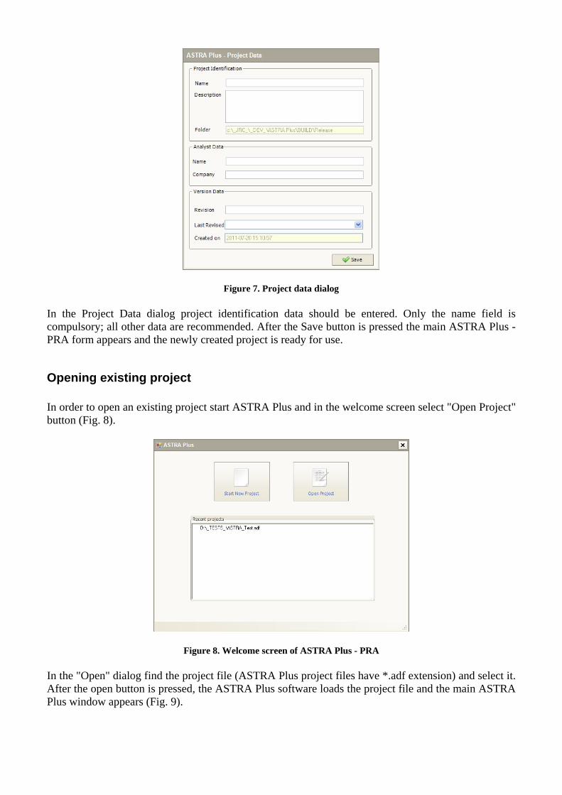
Figure 7. Project data dialog In the Project Data dialog project identification data should be entered. Only the name field is compulsory; all other data are recommended. After the Save button is pressed the main ASTRA Plus - PRA form appears and the newly created project is ready for use.

Opening existing project In order to open an existing project start ASTRA Plus and in the welcome screen select "Open Project" button (Fig. 8).

Figure 8. Welcome screen of ASTRA Plus - PRA In the "Open" dialog find the project file (ASTRA Plus project files have *.adf extension) and select it. After the open button is pressed, the ASTRA Plus software loads the project file and the main ASTRA Plus window appears (Fig. 9).

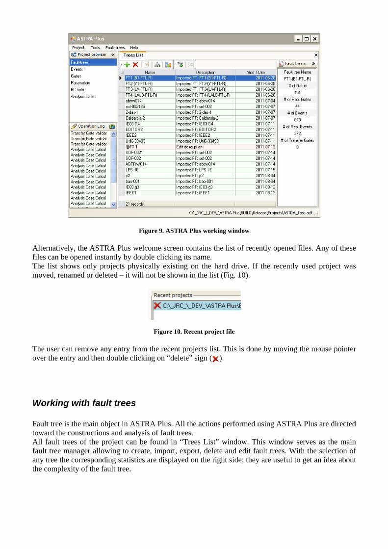
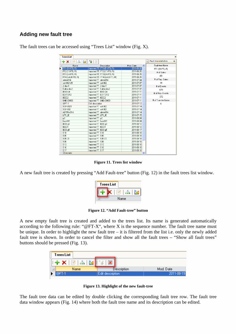
Figure 9. ASTRA Plus working window Alternatively, the ASTRA Plus welcome screen contains the list of recently opened files. Any of these files can be opened instantly by double clicking its name. The list shows only projects physically existing on the hard drive. If the recently used project was moved, renamed or deleted – it will not be shown in the list (Fig. 10).

Figure 10. Recent project file The user can remove any entry from the recent projects list. This is done by moving the mouse pointer over the entry and then double clicking on “delete” sign ( ).

Working with fault trees Fault tree is the main object in ASTRA Plus. All the actions performed using ASTRA Plus are directed toward the constructions and analysis of fault trees. All fault trees of the project can be found in “Trees List” window. This window serves as the main fault tree manager allowing to create, import, export, delete and edit fault trees. With the selection of any tree the corresponding statistics are displayed on the right side; they are useful to get an idea about the complexity of the fault tree.

Adding new fault tree The fault trees can be accessed using “Trees List” window (Fig. X).

Figure 11. Trees list window A new fault tree is created by pressing “Add Fault-tree” button (Fig. 12) in the fault trees list window.

Figure 12. “Add Fault-tree” button A new empty fault tree is created and added to the trees list. Its name is generated automatically according to the following rule: “@FT-X“, where X is the sequence number. The fault tree name must be unique. In order to highlight the new fault tree – it is filtered from the list i.e. only the newly added fault tree is shown. In order to cancel the filter and show all the fault trees – “Show all fault trees” buttons should be pressed (Fig. 13).

Figure 13. Highlight of the new fault-tree The fault tree data can be edited by double clicking the corresponding fault tree row. The fault tree data window appears (Fig. 14) where both the fault tree name and its description can be edited.

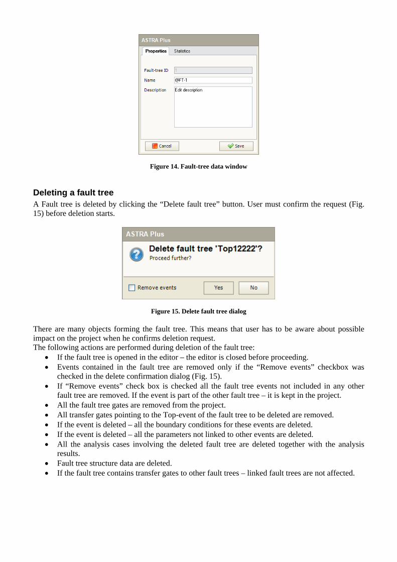
Figure 14. Fault-tree data window

Deleting a fault tree A Fault tree is deleted by clicking the “Delete fault tree” button. User must confirm the request (Fig. 15) before deletion starts.

Figure 15. Delete fault tree dialog There are many objects forming the fault tree. This means that user has to be aware about possible impact on the project when he confirms deletion request. The following actions are performed during deletion of the fault tree:

• If the fault tree is opened in the editor – the editor is closed before proceeding. • Events contained in the fault tree are removed only if the “Remove events” checkbox was

checked in the delete confirmation dialog (Fig. 15). • If “Remove events” check box is checked all the fault tree events not included in any other

fault tree are removed. If the event is part of the other fault tree – it is kept in the project. • All the fault tree gates are removed from the project. • All transfer gates pointing to the Top-event of the fault tree to be deleted are removed. • If the event is deleted – all the boundary conditions for these events are deleted. • If the event is deleted – all the parameters not linked to other events are deleted. • All the analysis cases involving the deleted fault tree are deleted together with the analysis

results. • Fault tree structure data are deleted. • If the fault tree contains transfer gates to other fault trees – linked fault trees are not affected.

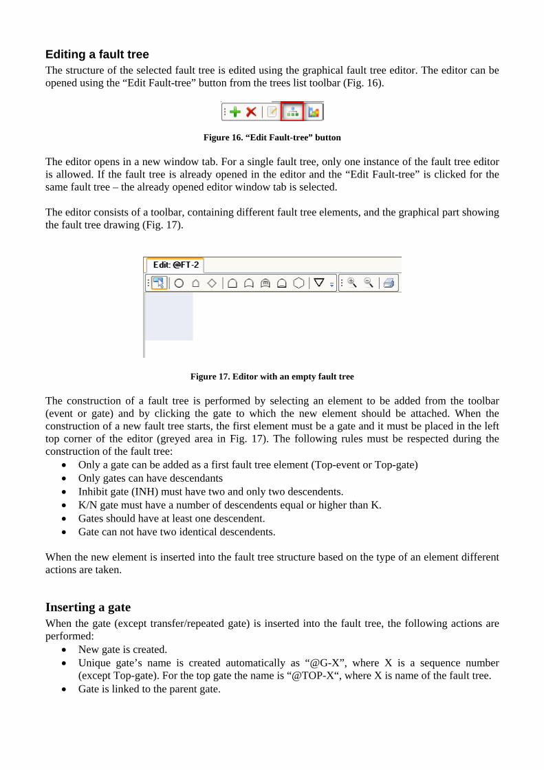
Editing a fault tree The structure of the selected fault tree is edited using the graphical fault tree editor. The editor can be opened using the “Edit Fault-tree” button from the trees list toolbar (Fig. 16).

Figure 16. “Edit Fault-tree” button The editor opens in a new window tab. For a single fault tree, only one instance of the fault tree editor is allowed. If the fault tree is already opened in the editor and the “Edit Fault-tree” is clicked for the same fault tree – the already opened editor window tab is selected. The editor consists of a toolbar, containing different fault tree elements, and the graphical part showing the fault tree drawing (Fig. 17).

Figure 17. Editor with an empty fault tree The construction of a fault tree is performed by selecting an element to be added from the toolbar (event or gate) and by clicking the gate to which the new element should be attached. When the construction of a new fault tree starts, the first element must be a gate and it must be placed in the left top corner of the editor (greyed area in Fig. 17). The following rules must be respected during the construction of the fault tree:

• Only a gate can be added as a first fault tree element (Top-event or Top-gate) • Only gates can have descendants • Inhibit gate (INH) must have two and only two descendents. • K/N gate must have a number of descendents equal or higher than K. • Gates should have at least one descendent. • Gate can not have two identical descendents.

When the new element is inserted into the fault tree structure based on the type of an element different actions are taken.

Inserting a gate When the gate (except transfer/repeated gate) is inserted into the fault tree, the following actions are performed:

• New gate is created. • Unique gate’s name is created automatically as “@G-X”, where X is a sequence number

(except Top-gate). For the top gate the name is “@TOP-X“, where X is name of the fault tree. • Gate is linked to the parent gate.

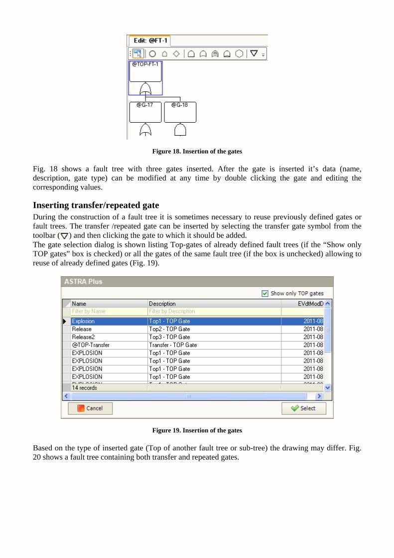
Figure 18. Insertion of the gates Fig. 18 shows a fault tree with three gates inserted. After the gate is inserted it’s data (name, description, gate type) can be modified at any time by double clicking the gate and editing the corresponding values.

Inserting transfer/repeated gate During the construction of a fault tree it is sometimes necessary to reuse previously defined gates or fault trees. The transfer /repeated gate can be inserted by selecting the transfer gate symbol from the toolbar ( ) and then clicking the gate to which it should be added. The gate selection dialog is shown listing Top-gates of already defined fault trees (if the “Show only TOP gates” box is checked) or all the gates of the same fault tree (if the box is unchecked) allowing to reuse of already defined gates (Fig. 19).

Figure 19. Insertion of the gates Based on the type of inserted gate (Top of another fault tree or sub-tree) the drawing may differ. Fig. 20 shows a fault tree containing both transfer and repeated gates.

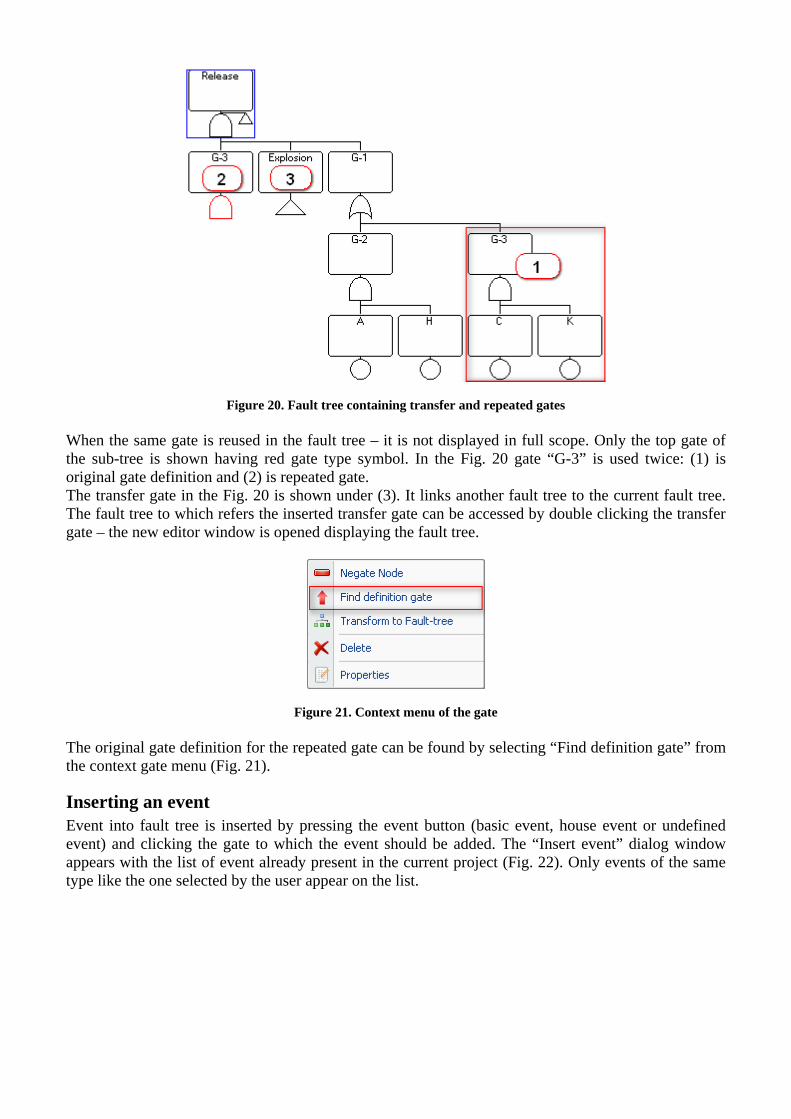
Figure 20. Fault tree containing transfer and repeated gates When the same gate is reused in the fault tree – it is not displayed in full scope. Only the top gate of the sub-tree is shown having red gate type symbol. In the Fig. 20 gate “G-3” is used twice: (1) is original gate definition and (2) is repeated gate. The transfer gate in the Fig. 20 is shown under (3). It links another fault tree to the current fault tree. The fault tree to which refers the inserted transfer gate can be accessed by double clicking the transfer gate – the new editor window is opened displaying the fault tree.

Figure 21. Context menu of the gate

The original gate definition for the repeated gate can be found by selecting “Find definition gate” from the context gate menu (Fig. 21).

Inserting an event Event into fault tree is inserted by pressing the event button (basic event, house event or undefined event) and clicking the gate to which the event should be added. The “Insert event” dialog window appears with the list of event already present in the current project (Fig. 22). Only events of the same type like the one selected by the user appear on the list.

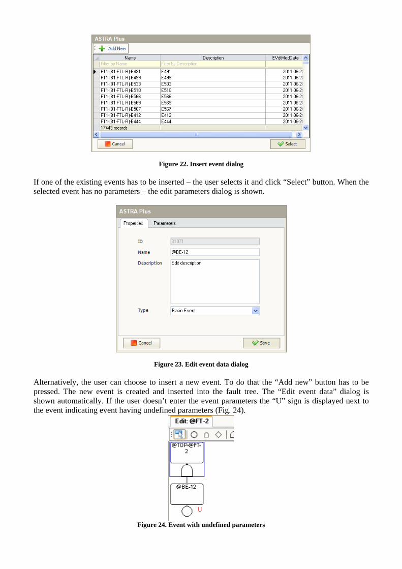
Figure 22. Insert event dialog If one of the existing events has to be inserted – the user selects it and click “Select” button. When the selected event has no parameters – the edit parameters dialog is shown.

Figure 23. Edit event data dialog Alternatively, the user can choose to insert a new event. To do that the “Add new” button has to be pressed. The new event is created and inserted into the fault tree. The “Edit event data” dialog is shown automatically. If the user doesn’t enter the event parameters the “U” sign is displayed next to the event indicating event having undefined parameters (Fig. 24).

Figure 24. Event with undefined parameters

Editing event/gate Events and gates can be edited by double-clicking the selected event/gate. The “Edit event” dialog appears. Depending on the type of event/gate different fields/properties are shown in this dialog. First tab “Properties” (Fig. 23) allows to edit name, description and type of event/gate. For some types of events and gates additional fields can be accessed:

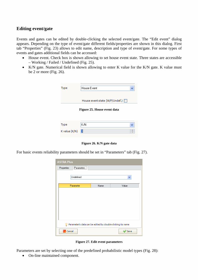
• House event. Check box is shown allowing to set house event state. Three states are accessible – Working / Failed / Undefined (Fig. 25).

• K/N gate. Numerical field is shown allowing to enter K value for the K/N gate. K value must be 2 or more (Fig. 26).

Figure 25. House event data

Figure 26. K/N gate data

For basic events reliability parameters should be set in “Parameters” tab (Fig. 27).

Figure 27. Edit event parameters Parameters are set by selecting one of the predefined probabilistic model types (Fig. 28):

• On-line maintained component.

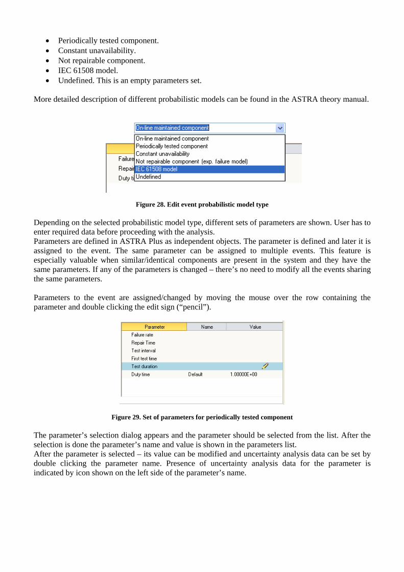
• Periodically tested component. • Constant unavailability. • Not repairable component. • IEC 61508 model. • Undefined. This is an empty parameters set.

More detailed description of different probabilistic models can be found in the ASTRA theory manual.

Figure 28. Edit event probabilistic model type Depending on the selected probabilistic model type, different sets of parameters are shown. User has to enter required data before proceeding with the analysis. Parameters are defined in ASTRA Plus as independent objects. The parameter is defined and later it is assigned to the event. The same parameter can be assigned to multiple events. This feature is especially valuable when similar/identical components are present in the system and they have the same parameters. If any of the parameters is changed – there’s no need to modify all the events sharing the same parameters. Parameters to the event are assigned/changed by moving the mouse over the row containing the parameter and double clicking the edit sign (“pencil”).

Figure 29. Set of parameters for periodically tested component The parameter’s selection dialog appears and the parameter should be selected from the list. After the selection is done the parameter’s name and value is shown in the parameters list. After the parameter is selected – its value can be modified and uncertainty analysis data can be set by double clicking the parameter name. Presence of uncertainty analysis data for the parameter is indicated by icon shown on the left side of the parameter’s name.

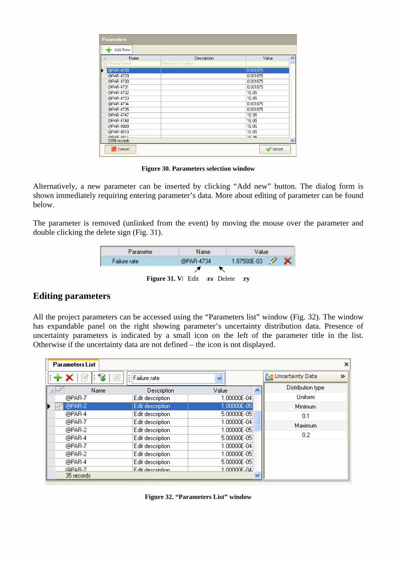
Figure 30. Parameters selection window Alternatively, a new parameter can be inserted by clicking “Add new” button. The dialog form is shown immediately requiring entering parameter’s data. More about editing of parameter can be found below. The parameter is removed (unlinked from the event) by moving the mouse over the parameter and double clicking the delete sign (Fig. 31).

Figure 31. View of parameters entry

Editing parameters All the project parameters can be accessed using the “Parameters list” window (Fig. 32). The window has expandable panel on the right showing parameter’s uncertainty distribution data. Presence of uncertainty parameters is indicated by a small icon on the left of the parameter title in the list. Otherwise if the uncertainty data are not defined – the icon is not displayed.

Figure 32. “Parameters List” window

Edit Delete

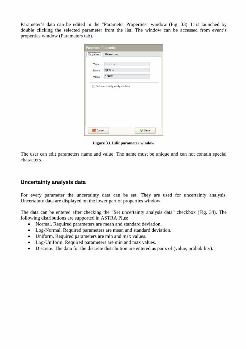
Parameter’s data can be edited in the “Parameter Properties” window (Fig. 33). It is launched by double clicking the selected parameter from the list. The window can be accessed from event’s properties window (Parameters tab).

Figure 33. Edit parameter window The user can edit parameters name and value. The name must be unique and can not contain special characters.

Uncertainty analysis data For every parameter the uncertainty data can be set. They are used for uncertainty analysis. Uncertainty data are displayed on the lower part of properties window. The data can be entered after checking the “Set uncertainty analysis data” checkbox (Fig. 34). The following distributions are supported in ASTRA Plus:

• Normal. Required parameters are mean and standard deviation. • Log-Normal. Required parameters are mean and standard deviation. • Uniform. Required parameters are min and max values. • Log-Uniform. Required parameters are min and max values. • Discrete. The data for the discrete distribution are entered as pairs of (value, probability).

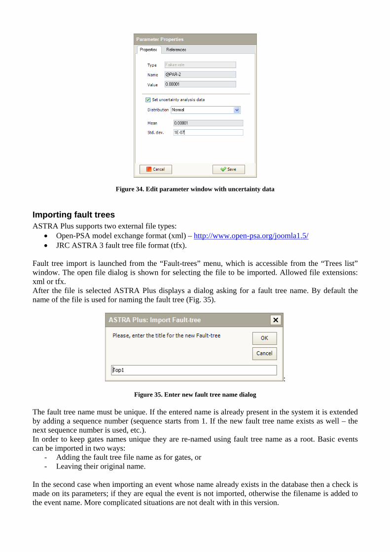
Figure 34. Edit parameter window with uncertainty data

Importing fault trees ASTRA Plus supports two external file types:

• Open-PSA model exchange format (xml) – http://www.open-psa.org/joomla1.5/ • JRC ASTRA 3 fault tree file format (tfx).

Fault tree import is launched from the “Fault-trees” menu, which is accessible from the “Trees list” window. The open file dialog is shown for selecting the file to be imported. Allowed file extensions: xml or tfx. After the file is selected ASTRA Plus displays a dialog asking for a fault tree name. By default the name of the file is used for naming the fault tree (Fig. 35).

:

Figure 35. Enter new fault tree name dialog The fault tree name must be unique. If the entered name is already present in the system it is extended by adding a sequence number (sequence starts from 1. If the new fault tree name exists as well – the next sequence number is used, etc.). In order to keep gates names unique they are re-named using fault tree name as a root. Basic events can be imported in two ways:

- Adding the fault tree file name as for gates, or - Leaving their original name.

In the second case when importing an event whose name already exists in the database then a check is made on its parameters; if they are equal the event is not imported, otherwise the filename is added to the event name. More complicated situations are not dealt with in this version.

Exporting fault trees ASTRA Plus can export fault trees using two file types:

• Open-PSA model exchange format (xml); • JRC ASTRA 3 fault tree file format (tfx).

Fault tree export is launched from the “Fault-trees” menu, which is accessible from the “Trees list” window. The save file dialog is shown for indication of the destination file. In the dialog the type of file can be selected (xml or tfx). After the save button is pressed the export of the fault tree is executed.

Analysing fault trees Fault tree analysis is performed by creating Analysis cases. An analysis case is a collection of different analysis settings and assumptions used during the fault tree analysis. An analysis case is created from the Analysis cases list by pressing “Add Analysis Case” button (Fig. 36).

Figure 36. Add analysis case button An analysis case is defined in several steps using the “Create Analysis Case” dialog. During the first step (Fig. 37) the preferred analysis type can be selected. The selection can be done from three types:

• Exact BDD analysis. • Approximated TZBDD analysis. • Decomposition.

The second step is the selection of the fault tree to be analysed. ASTRA Plus lists all the available fault trees and the user has to select the one to be analysed (Fig. 38).

Figure 37. Create analysis case. Step 1: selection of analysis type

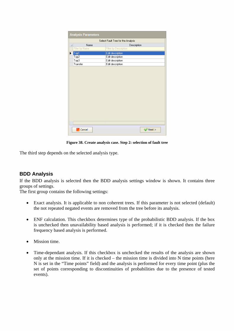
Figure 38. Create analysis case. Step 2: selection of fault tree The third step depends on the selected analysis type.

BDD Analysis If the BDD analysis is selected then the BDD analysis settings window is shown. It contains three groups of settings. The first group contains the following settings:

• Exact analysis. It is applicable to non coherent trees. If this parameter is not selected (default) the not repeated negated events are removed from the tree before its analysis.

• ENF calculation. This checkbox determines type of the probabilistic BDD analysis. If the box is unchecked then unavailability based analysis is performed; if it is checked then the failure frequency based analysis is performed.

• Mission time.

• Time-dependant analysis. If this checkbox is unchecked the results of the analysis are shown

only at the mission time. If it is checked – the mission time is divided into N time points (here N is set in the “Time points” field) and the analysis is performed for every time point (plus the set of points corresponding to discontinuities of probabilities due to the presence of tested events).

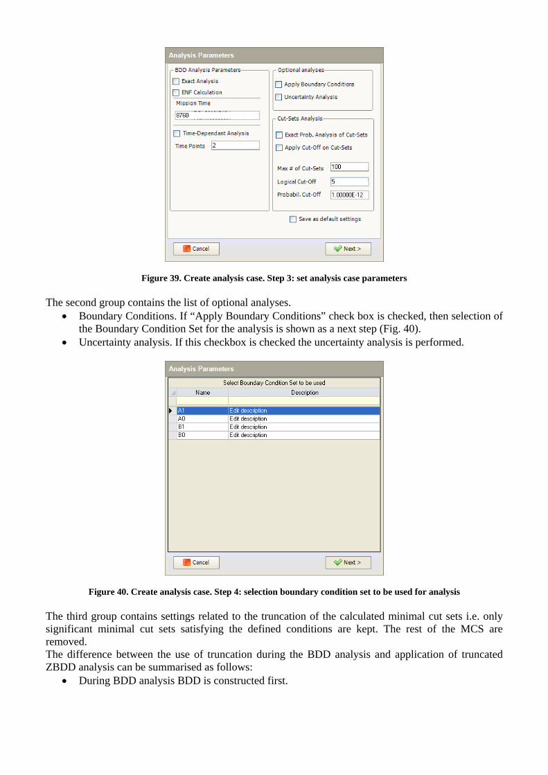
Figure 39. Create analysis case. Step 3: set analysis case parameters The second group contains the list of optional analyses.

• Boundary Conditions. If “Apply Boundary Conditions” check box is checked, then selection of the Boundary Condition Set for the analysis is shown as a next step (Fig. 40).

• Uncertainty analysis. If this checkbox is checked the uncertainty analysis is performed.

Figure 40. Create analysis case. Step 4: selection boundary condition set to be used for analysis

The third group contains settings related to the truncation of the calculated minimal cut sets i.e. only significant minimal cut sets satisfying the defined conditions are kept. The rest of the MCS are removed. The difference between the use of truncation during the BDD analysis and application of truncated ZBDD analysis can be summarised as follows:

• During BDD analysis BDD is constructed first.

• All the minimal cut sets are determined by reducing the BDD to the ZBDD. The truncation is applied during the reduction process. Thus if the BDD can not be constructed then the MCS can not be determined as well.

TZBDD Analysis Truncated BDD is used when, due to the insufficient computational resources and high complexity of the fault tree, the BDD cannot be constructed. The truncated BDD (TZBDD) is constructed directly by applying the truncation method. Only the unavailability analysis is performed on the TZBDD. It should be noted that TZBDD is an approximate analysis. Because of the application of truncation only upper bound unavailability (using rare event approximation) is calculated.

Figure 41. Create analysis case. Step 3: setting parameters for TZBDD analysis The main settings for TZBDD analysis are related to the truncation threshold:

• Maximal number of MCS • Maximal order of MCS • Probabilistic threshold for the MCS. If the MCS probability is less than the defined threshold –

the MCS is removed. Note. The truncation threshold should be carefully selected. The analyst must be sure that the steady state for the Top-event unavailability has been reached.

Decomposition analysis When the exact analysis for the complex fault tree can not be performed using BDD and the approximate results are not acceptable – decomposition method can be used. Decomposition allows to obtain exact Top-event probability by splitting (decomposing) the complex fault tree into a set of simpler trees and then analysing them using BDD. Only the unavailability analysis is performed with the decomposition method.

The main decomposition parameter is maximum decomposition depth. When the simpler fault tree obtained during the decomposition is still too complex to be analysed using BDD – the same decomposition procedure can be applied to it. Thus we obtain second decomposition depth. The maximal decomposition depth parameter determines how many times we can apply the decomposition method for simpler fault trees.

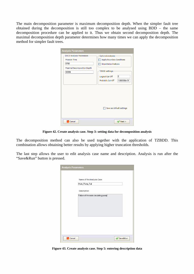
Figure 42. Create analysis case. Step 3: setting data for decomposition analysis The decomposition method can also be used together with the application of TZBDD. This combination allows obtaining better results by applying higher truncation thresholds. The last step allows the user to edit analysis case name and description. Analysis is run after the “Save&Run” button is pressed.

Figure 43. Create analysis case. Step 5: entering description data

When the user creates the analysis case and confirms it by pressing “Save&Run” button, the calculations starts. During calculation the analysis module is shown (Fig. 44).

Figure 44. Analysis module After the calculations are finished the analysis module disappears and the results for the selected analysis case are displayed. Alternatively, the analysis case for the selected fault tree can be created from the fault tree list window by pressing “Create new analysis case” button (Fig. X).

Figure 45. Create analysis case

This opens the Analysis case list window and launches the analysis case wizard for the selected fault tree. Because the fault tree is already selected – the fault tree selection step is skipped.

Viewing analysis results When the analysis case is selected in the analysis case list the status of the calculations is displayed in the lower part of the window under the “Summary of Analysis results”. If the calculation was performed successfully then the main probabilistic results are provided (Fig. 46).

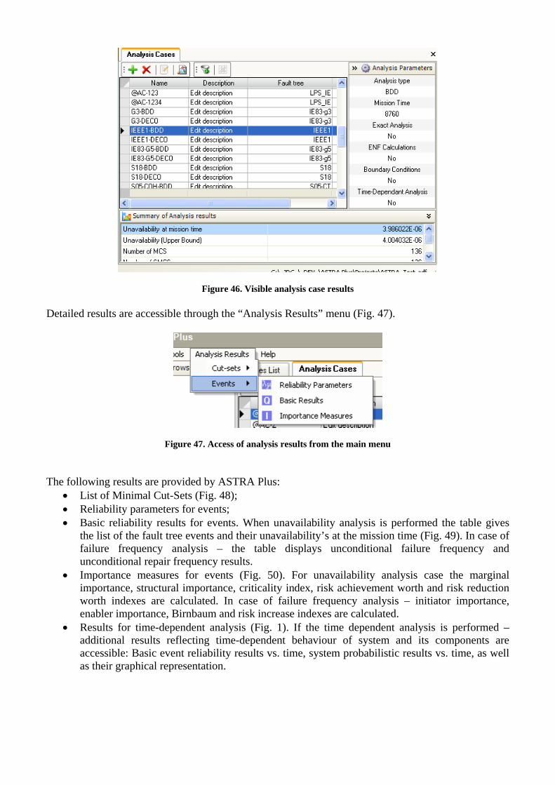
Figure 46. Visible analysis case results Detailed results are accessible through the “Analysis Results” menu (Fig. 47).

Figure 47. Access of analysis results from the main menu The following results are provided by ASTRA Plus:

• List of Minimal Cut-Sets (Fig. 48); • Reliability parameters for events; • Basic reliability results for events. When unavailability analysis is performed the table gives

the list of the fault tree events and their unavailability’s at the mission time (Fig. 49). In case of failure frequency analysis – the table displays unconditional failure frequency and unconditional repair frequency results.

• Importance measures for events (Fig. 50). For unavailability analysis case the marginal importance, structural importance, criticality index, risk achievement worth and risk reduction worth indexes are calculated. In case of failure frequency analysis – initiator importance, enabler importance, Birnbaum and risk increase indexes are calculated.

• Results for time-dependent analysis (Fig. 1). If the time dependent analysis is performed – additional results reflecting time-dependent behaviour of system and its components are accessible: Basic event reliability results vs. time, system probabilistic results vs. time, as well as their graphical representation.

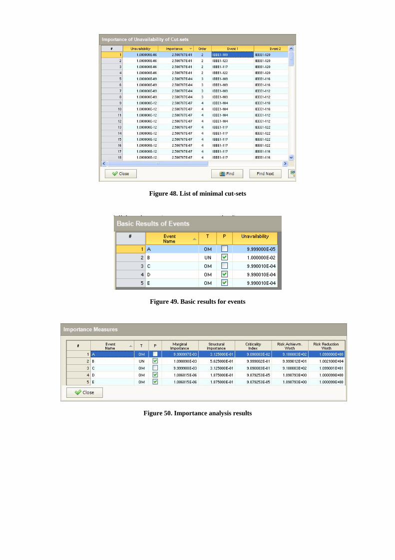
Figure 48. List of minimal cut-sets

Figure 49. Basic results for events

Figure 50. Importance analysis results

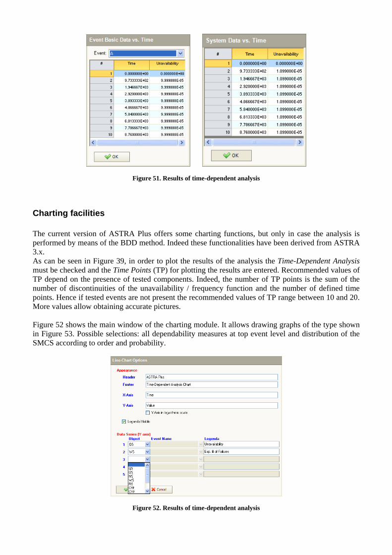
Figure 51. Results of time-dependent analysis

Charting facilities The current version of ASTRA Plus offers some charting functions, but only in case the analysis is performed by means of the BDD method. Indeed these functionalities have been derived from ASTRA 3.x. As can be seen in Figure 39, in order to plot the results of the analysis the Time-Dependent Analysis must be checked and the Time Points (TP) for plotting the results are entered. Recommended values of TP depend on the presence of tested components. Indeed, the number of TP points is the sum of the number of discontinuities of the unavailability / frequency function and the number of defined time points. Hence if tested events are not present the recommended values of TP range between 10 and 20. More values allow obtaining accurate pictures. Figure 52 shows the main window of the charting module. It allows drawing graphs of the type shown in Figure 53. Possible selections: all dependability measures at top event level and distribution of the SMCS according to order and probability.

Figure 52. Results of time-dependent analysis

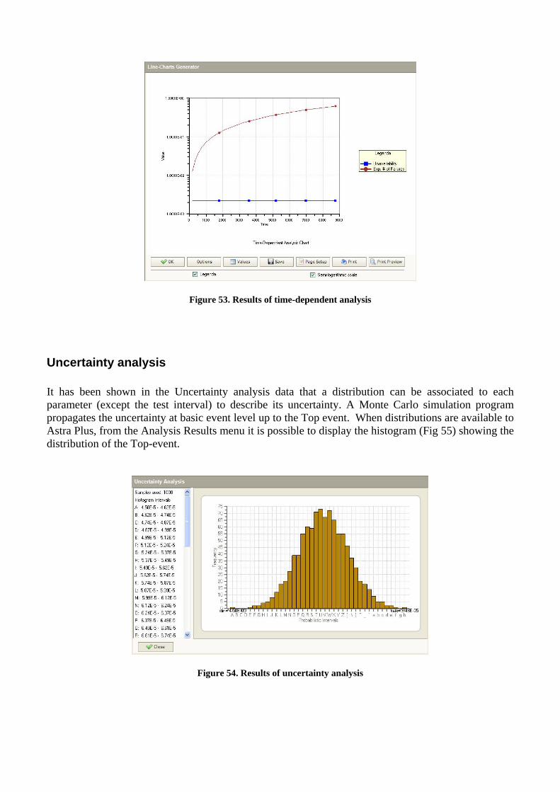
Figure 53. Results of time-dependent analysis

Uncertainty analysis It has been shown in the Uncertainty analysis data that a distribution can be associated to each parameter (except the test interval) to describe its uncertainty. A Monte Carlo simulation program propagates the uncertainty at basic event level up to the Top event. When distributions are available to Astra Plus, from the Analysis Results menu it is possible to display the histogram (Fig 55) showing the distribution of the Top-event.

Figure 54. Results of uncertainty analysis

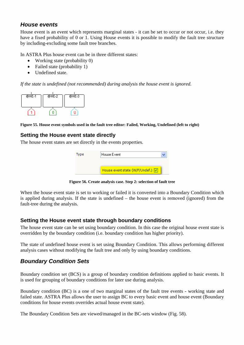
House events House event is an event which represents marginal states - it can be set to occur or not occur, i.e. they have a fixed probability of 0 or 1. Using House events it is possible to modify the fault tree structure by including-excluding some fault tree branches. In ASTRA Plus house event can be in three different states:

• Working state (probability 0) • Failed state (probability 1) • Undefined state.

If the state is undefined (not recommended) during analysis the house event is ignored.

Figure 55. House event symbols used in the fault tree editor: Failed, Working, Undefined (left to right)

Setting the House event state directly The house event states are set directly in the events properties.

Figure 56. Create analysis case. Step 2: selection of fault tree When the house event state is set to working or failed it is converted into a Boundary Condition which is applied during analysis. If the state is undefined – the house event is removed (ignored) from the fault-tree during the analysis.

Setting the House event state through boundary conditions The house event state can be set using boundary condition. In this case the original house event state is overridden by the boundary condition (i.e. boundary condition has higher priority). The state of undefined house event is set using Boundary Condition. This allows performing different analysis cases without modifying the fault tree and only by using boundary conditions.

Boundary Condition Sets Boundary condition set (BCS) is a group of boundary condition definitions applied to basic events. It is used for grouping of boundary conditions for later use during analysis. Boundary condition (BC) is a one of two marginal states of the fault tree events - working state and failed state. ASTRA Plus allows the user to assign BC to every basic event and house event (Boundary conditions for house events overrides actual house event state). The Boundary Condition Sets are viewed/managed in the BC-sets window (Fig. 58).

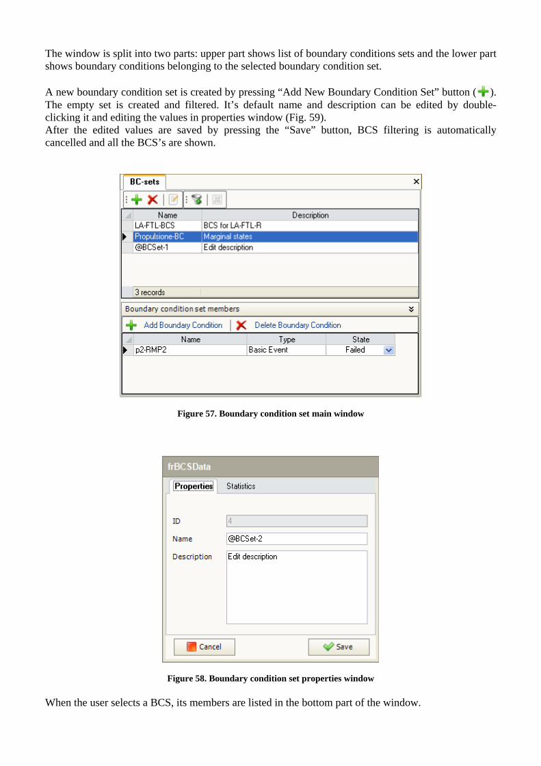
The window is split into two parts: upper part shows list of boundary conditions sets and the lower part shows boundary conditions belonging to the selected boundary condition set. A new boundary condition set is created by pressing “Add New Boundary Condition Set” button ( ). The empty set is created and filtered. It’s default name and description can be edited by double-clicking it and editing the values in properties window (Fig. 59). After the edited values are saved by pressing the “Save” button, BCS filtering is automatically cancelled and all the BCS’s are shown.

Figure 57. Boundary condition set main window

Figure 58. Boundary condition set properties window When the user selects a BCS, its members are listed in the bottom part of the window.

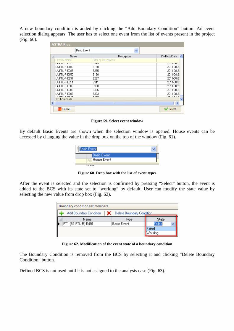
A new boundary condition is added by clicking the “Add Boundary Condition” button. An event selection dialog appears. The user has to select one event from the list of events present in the project (Fig. 60).

Figure 59. Select event window By default Basic Events are shown when the selection window is opened. House events can be accessed by changing the value in the drop box on the top of the window (Fig. 61).

Figure 60. Drop box with the list of event types After the event is selected and the selection is confirmed by pressing “Select” button, the event is added to the BCS with its state set to “working” by default. User can modify the state value by selecting the new value from drop box (Fig. 62).

Figure 62. Modification of the event state of a boundary condition The Boundary Condition is removed from the BCS by selecting it and clicking “Delete Boundary Condition” button. Defined BCS is not used until it is not assigned to the analysis case (Fig. 63).

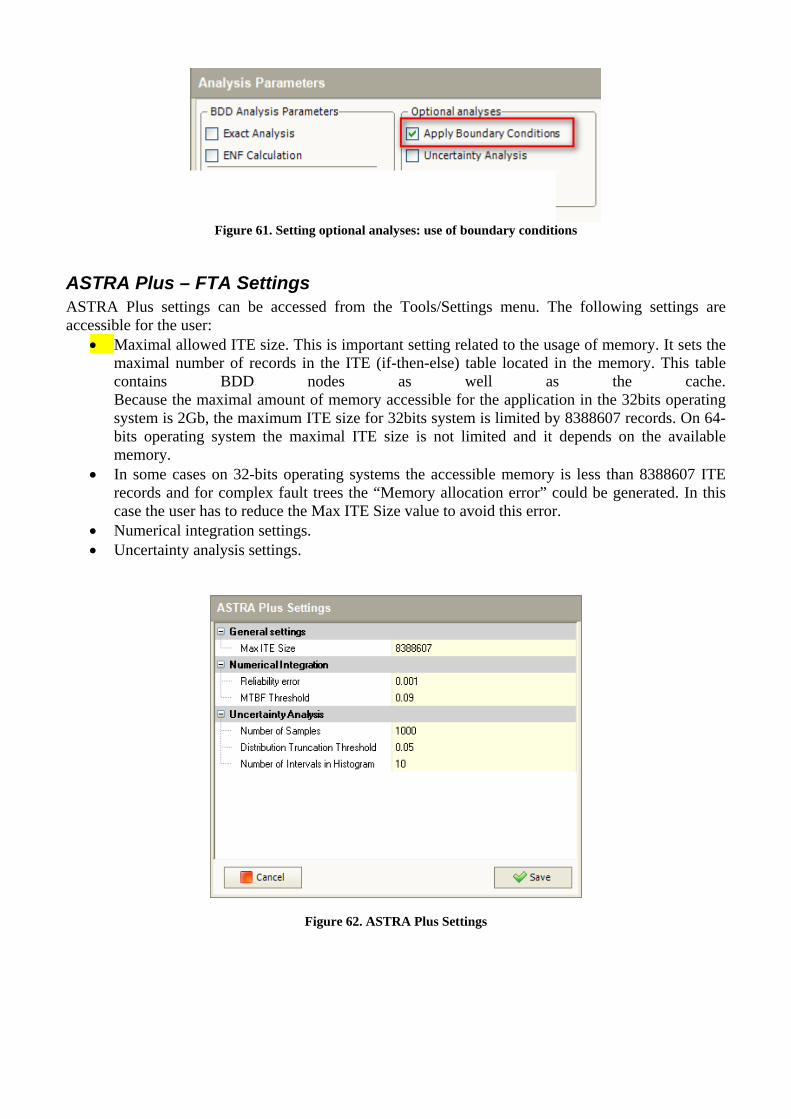
Figure 61. Setting optional analyses: use of boundary conditions

ASTRA Plus – FTA Settings ASTRA Plus settings can be accessed from the Tools/Settings menu. The following settings are accessible for the user:

• Maximal allowed ITE size. This is important setting related to the usage of memory. It sets the maximal number of records in the ITE (if-then-else) table located in the memory. This table contains BDD nodes as well as the cache. Because the maximal amount of memory accessible for the application in the 32bits operating system is 2Gb, the maximum ITE size for 32bits system is limited by 8388607 records. On 64-bits operating system the maximal ITE size is not limited and it depends on the available memory.

• In some cases on 32-bits operating systems the accessible memory is less than 8388607 ITE records and for complex fault trees the “Memory allocation error” could be generated. In this case the user has to reduce the Max ITE Size value to avoid this error.

• Numerical integration settings. • Uncertainty analysis settings.

Figure 62. ASTRA Plus Settings

The CISA module of ASTRA Plus The CISA module allows performing Importance and sensitivity analysis on all fault trees describing events with significant consequences. The fault tree analysis gives the top-event unavailability / unreliability upper bound which are compared with target values defined by or imposed to the analyst. Top events that do not meet the target are submitted to the Concurrent Importance and Sensitivity Analysis in order to identify the set of feasible design solutions from which the one to be implemented is selected on the basis of cost-effective design considerations. The theory implemented in ASTRA-CISA is described in several documents, from ref [8] to ref [12]. The following description refers to version 1.0 of the CISA module. The input of CISA is the project already prepared using the FTA module of ASTRA Plus. It is recommended to read at least ref [8] before using this module.

Software Interface The graphical user interface of the CISA module of ASTRA Plus is designed to be simple and intuitive. There are two different interfaces:

• Welcome screen; • Working screen.

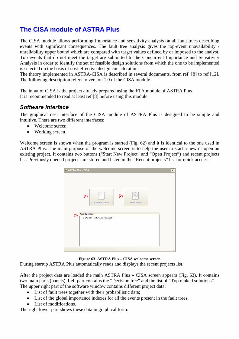
Welcome screen is shown when the program is started (Fig. 62) and it is identical to the one used in ASTRA Plus. The main purpose of the welcome screen is to help the user to start a new or open an existing project. It contains two buttons (“Start New Project” and “Open Project”) and recent projects list. Previously opened projects are stored and listed in the “Recent projects” list for quick access.

Figure 63. ASTRA Plus – CISA welcome screen During startup ASTRA Plus automatically reads and displays the recent projects list. After the project data are loaded the main ASTRA Plus – CISA screen appears (Fig. 63). It contains two main parts (panels). Left part contains the “Decision tree” and the list of “Top ranked solutions”. The upper right part of the software window contains different project data:

• List of fault trees together with their probabilistic data; • List of the global importance indexes for all the events present in the fault trees; • List of modifications.

The right lower part shows these data in graphical form.

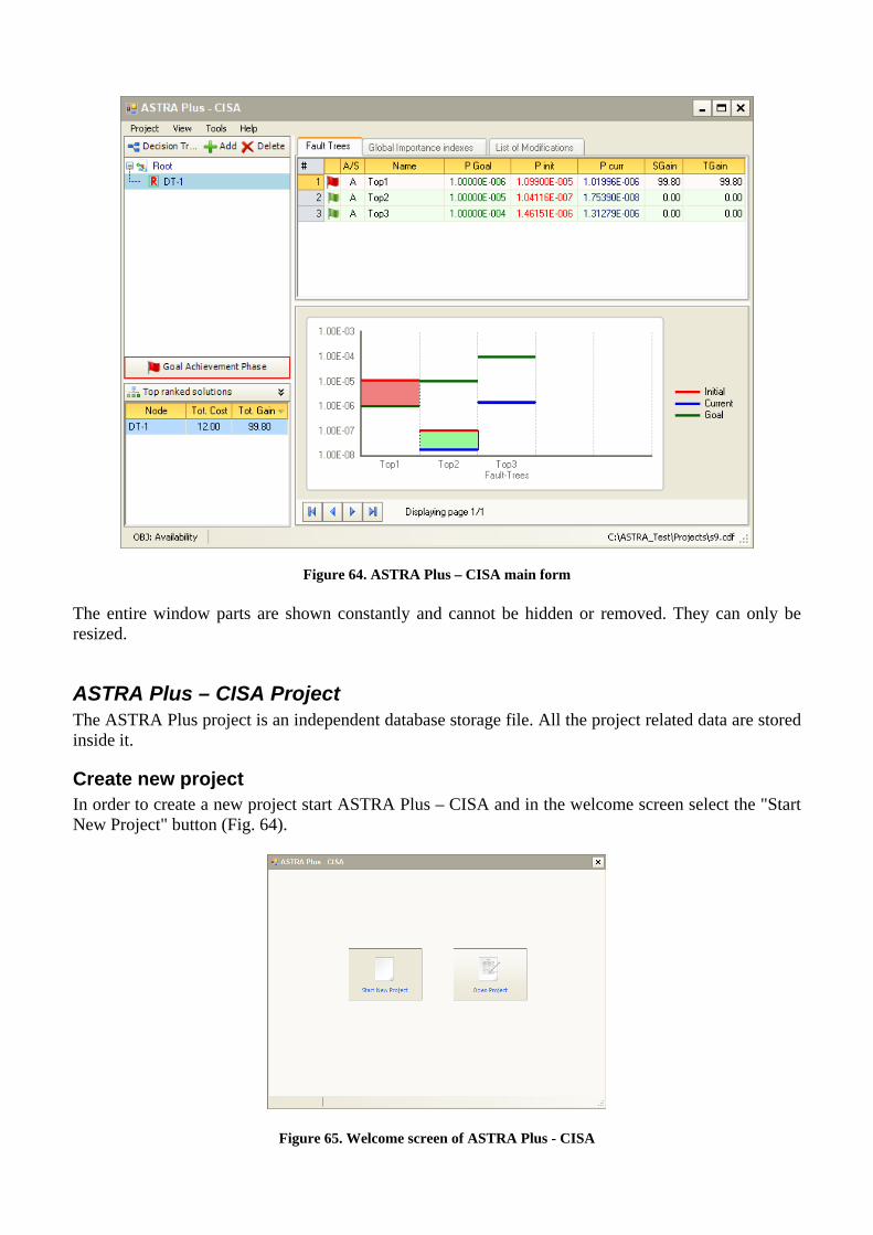
Figure 64. ASTRA Plus – CISA main form The entire window parts are shown constantly and cannot be hidden or removed. They can only be resized.

ASTRA Plus – CISA Project The ASTRA Plus project is an independent database storage file. All the project related data are stored inside it.

Create new project In order to create a new project start ASTRA Plus – CISA and in the welcome screen select the "Start New Project" button (Fig. 64).

Figure 65. Welcome screen of ASTRA Plus - CISA

The “Create New CISA Project” screen is shown (Fig. 65) where all the project input data and parameters should be entered:

• Analysis case name (required); • Detailed analysis case description (optional); • Analysis objective – Availability or Safety (required); • Mission time (required); • Location of the project file (required); • Location of the project data source – ASTRA Plus – PRA project file (required).

After all the input data are entered it is possible to proceed to the next step by pressing the “Next >” button. The ASTRA Plus project is loaded and the list of the available fault trees is displayed. It must be ensured that the ASTRA Plus project file is not used by other software instances (it is not read locked). The upper part of the window (see Figure 66) provides the list of the available fault trees loaded from the ASTRA project file (files with extension adf). By using add/remove buttons the fault trees are included / excluded into/from the CISA project. The fault trees included into CISA project are shown in the lower part of the screen. For every added fault tree the probabilistic goal value must be set. Fault trees without the probabilistic goal are highlighted. The “Next >” button can be pressed after the fault trees are selected and their probabilistic goals are set. It should be stressed that the later addition/removal of fault trees is not possible.

Figure 66. Create new CISA project dialog: Step 1

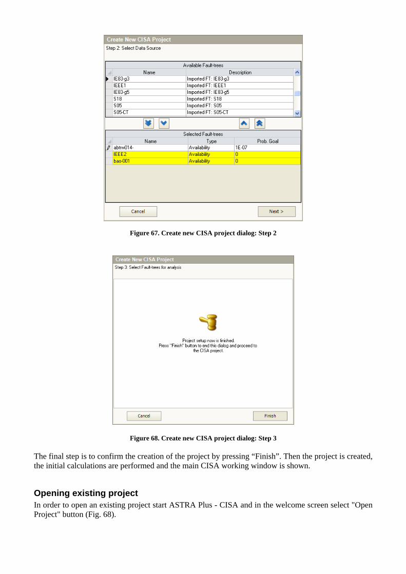
Figure 67. Create new CISA project dialog: Step 2

Figure 68. Create new CISA project dialog: Step 3 The final step is to confirm the creation of the project by pressing “Finish”. Then the project is created, the initial calculations are performed and the main CISA working window is shown.

Opening existing project In order to open an existing project start ASTRA Plus - CISA and in the welcome screen select "Open Project" button (Fig. 68).

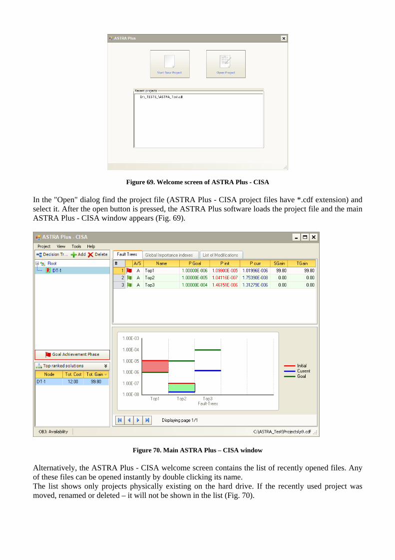
Figure 69. Welcome screen of ASTRA Plus - CISA In the "Open" dialog find the project file (ASTRA Plus - CISA project files have *.cdf extension) and select it. After the open button is pressed, the ASTRA Plus software loads the project file and the main ASTRA Plus - CISA window appears (Fig. 69).

Figure 70. Main ASTRA Plus – CISA window

Alternatively, the ASTRA Plus - CISA welcome screen contains the list of recently opened files. Any of these files can be opened instantly by double clicking its name. The list shows only projects physically existing on the hard drive. If the recently used project was moved, renamed or deleted – it will not be shown in the list (Fig. 70).

Figure 71. Recent project entry The user can remove any entry from the recent projects list. This is done by moving the mouse pointer over the entry and then double clicking the “delete” symbol ( ).

Working with ASTRA Plus – CISA project The Decision Tree (DT) is the main object in ASTRA Plus - CISA. All the actions performed using CISA are directed toward the analysis of different design modifications, which are compared through the quantification of the set of predefined fault trees. The best set of modifications satisfying the predefined goal conditions is identified as the result of the CISA analysis. The decision tree (DT) is always displayed on the left part of the working window (see Figure 71) and represents a hierarchical representation of design modifications. The DT always has at least one node, the “Root” node. This is the node representing the initial design (basic) solution of the system under analysis. Other DT nodes descend from the Root node.

Figure 72. Decision tree

Every node represents single system modification and all the nodes from the selected DT node to the Root node represent a set of modifications.

Adding new modification A new modification to the decision tree can be added by clicking he Add button located above the decision tree (Fig. 72).

Figure 73. Add modification button A new decision tree node will be added as a new descendant to the selected node. In order to enter all the necessary modification data the “Add Modification” dialog is used. The dialog consists of 3 or 4 different steps depending on the type of the modification. The initial dialog screen is used to select the type of the modification (Fig. 7) among the following:

• Modify parameters. This type of modification should be used when the analyst wants to substitute a single event/component with a different one.

• Use redundancy. This type of modification should be used when the analyst wants to substitute the selected component with a redundant configuration of components equal to the selected one.

• Advanced modification. When the above mentioned modifications are not sufficient or not feasible, then more advanced modifications are required with an impact on the fault tree structure. This type allows the analyst to directly modify the fault tree structure through the use of the graphical editor.

Figure 74: Selection of the modification type Note that the first two modifications do not change the fault tree structure, but only the parameters of the selected basic event. Consequently to substitute the component with a redundant configuration made up by components with different reliability data it is necessary to apply the first modification type and then the second one.

Modifying parameters If the “Modify parameters” type is selected then the next step consists of selecting the event for modification. In the dialog window the list of all events is displayed and user have to select one of them (Fig. 74). The events can be ordered in different ways. The order is done based on two criteria:

• Ordering of events is based on the active global importance measure. The name of the active importance measure is displayed on the column header showing global importance values.

• Events are ordered in the decreasing order (from the most important to the least important) in case of “Goal Achievement Phase”. In case of “Cost Reduction Phase” events are ordered in the ascending order (from the least important to the most important). The phase from one to another can be changed by using the button on the top of the table.

In order to proceed, press the “next” button. The third step allows user to change the parameters. There are two options:

• Only parameter values should be modified (e.g. a new component of the same type is installed having better availability property). When the mouse moves over the parameters two icons are shown – pencil for editing and cross for removal (Fig. 76). If the edit icon is double clicked then an input dialog is shown allowing entering new parameter value (Fig. 77).

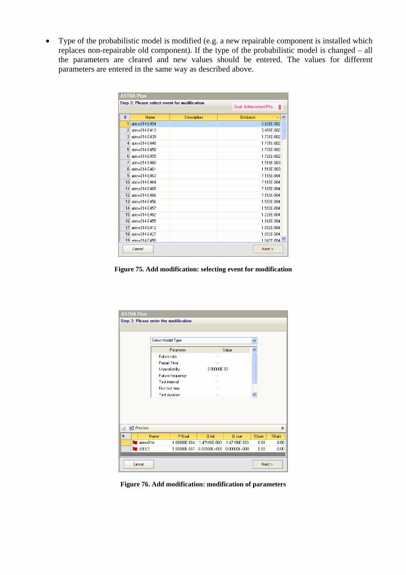
• Type of the probabilistic model is modified (e.g. a new repairable component is installed which replaces non-repairable old component). If the type of the probabilistic model is changed – all the parameters are cleared and new values should be entered. The values for different parameters are entered in the same way as described above.

Figure 75. Add modification: selecting event for modification

Figure 76. Add modification: modification of parameters

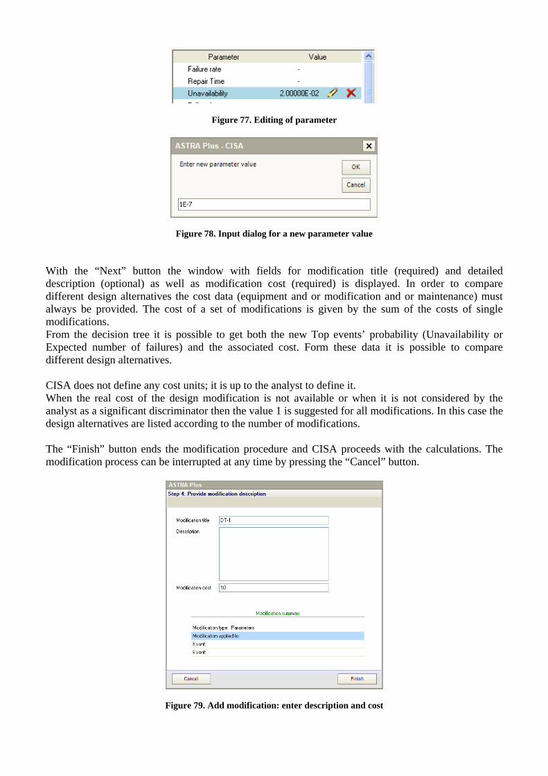
Figure 77. Editing of parameter

Figure 78. Input dialog for a new parameter value With the “Next” button the window with fields for modification title (required) and detailed description (optional) as well as modification cost (required) is displayed. In order to compare different design alternatives the cost data (equipment and or modification and or maintenance) must always be provided. The cost of a set of modifications is given by the sum of the costs of single modifications. From the decision tree it is possible to get both the new Top events’ probability (Unavailability or Expected number of failures) and the associated cost. Form these data it is possible to compare different design alternatives. CISA does not define any cost units; it is up to the analyst to define it. When the real cost of the design modification is not available or when it is not considered by the analyst as a significant discriminator then the value 1 is suggested for all modifications. In this case the design alternatives are listed according to the number of modifications. The “Finish” button ends the modification procedure and CISA proceeds with the calculations. The modification process can be interrupted at any time by pressing the “Cancel” button.

Figure 79. Add modification: enter description and cost

Adding redundancy If the “Add redundancy” type is selected then the next step consists of selecting the event for modification. In the dialog window the list of all events is displayed and the user has to select one of them (same as in case of parameters modification).

Figure 80. Add modification: enter redundancy data After the selection is done the redundancy data can be defined in the next step (Fig. 79). The redundancy is defined by selecting one of the predefined types (Fig. 80):

• Parallel redundancy; • K/N of active events; • Cold/Warm/Hot standby.

Figure 81. Input dialog for a new redundancy type After the redundancy type and its parameters are defined the calculations is activated by pressing the “Recalc” button (Fig. 79). The calculated unavailability value for the selected redundant configuration is displayed in the “Preview” area. Detailed equations for calculations of the redundancy configurations are provided in the theory manual. After all the redundancy data are entered it is possible to proceed to the last step where the modification title, description and cost is entered (For details see section on parameters modification).

Advanced modification This is the option for introduction of the most complicated modifications. Because effects of manually edited fault trees can be hardly predictable in case of presence of common events – it is strongly

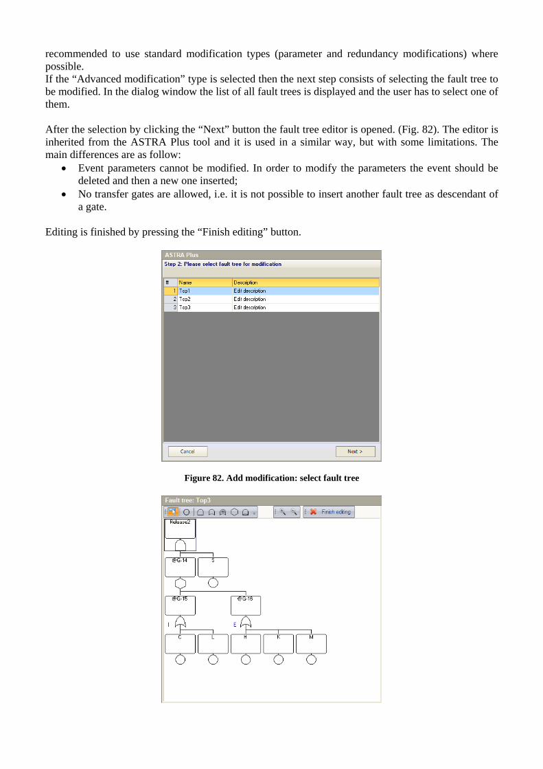
recommended to use standard modification types (parameter and redundancy modifications) where possible. If the “Advanced modification” type is selected then the next step consists of selecting the fault tree to be modified. In the dialog window the list of all fault trees is displayed and the user has to select one of them. After the selection by clicking the “Next” button the fault tree editor is opened. (Fig. 82). The editor is inherited from the ASTRA Plus tool and it is used in a similar way, but with some limitations. The main differences are as follow:

• Event parameters cannot be modified. In order to modify the parameters the event should be deleted and then a new one inserted;

• No transfer gates are allowed, i.e. it is not possible to insert another fault tree as descendant of a gate.

Editing is finished by pressing the “Finish editing” button.

Figure 82. Add modification: select fault tree

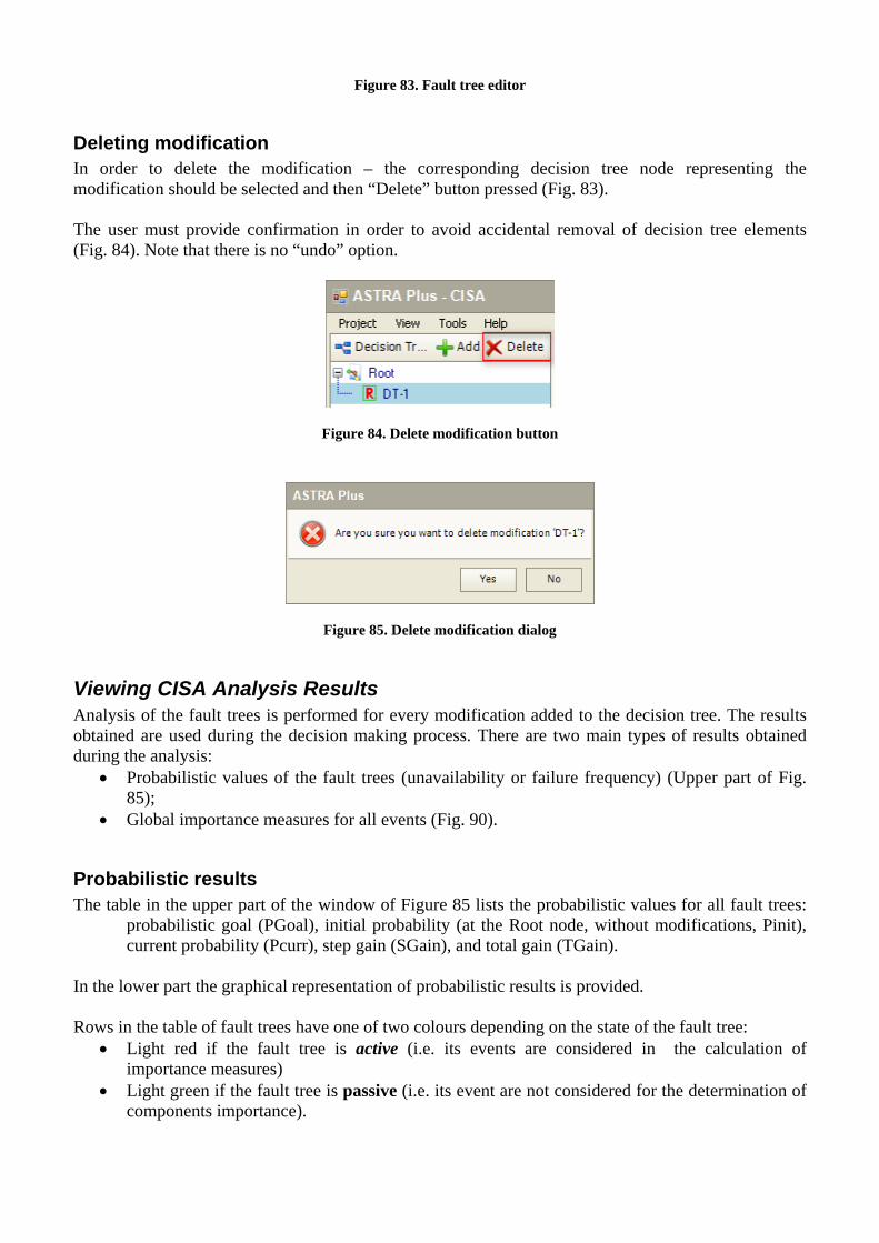
Figure 83. Fault tree editor

Deleting modification In order to delete the modification – the corresponding decision tree node representing the modification should be selected and then “Delete” button pressed (Fig. 83). The user must provide confirmation in order to avoid accidental removal of decision tree elements (Fig. 84). Note that there is no “undo” option.

Figure 84. Delete modification button

Figure 85. Delete modification dialog

Viewing CISA Analysis Results Analysis of the fault trees is performed for every modification added to the decision tree. The results obtained are used during the decision making process. There are two main types of results obtained during the analysis:

• Probabilistic values of the fault trees (unavailability or failure frequency) (Upper part of Fig. 85);

• Global importance measures for all events (Fig. 90).

Probabilistic results The table in the upper part of the window of Figure 85 lists the probabilistic values for all fault trees:

probabilistic goal (PGoal), initial probability (at the Root node, without modifications, Pinit), current probability (Pcurr), step gain (SGain), and total gain (TGain).

In the lower part the graphical representation of probabilistic results is provided. Rows in the table of fault trees have one of two colours depending on the state of the fault tree:

• Light red if the fault tree is active (i.e. its events are considered in the calculation of importance measures)

• Light green if the fault tree is passive (i.e. its event are not considered for the determination of components importance).

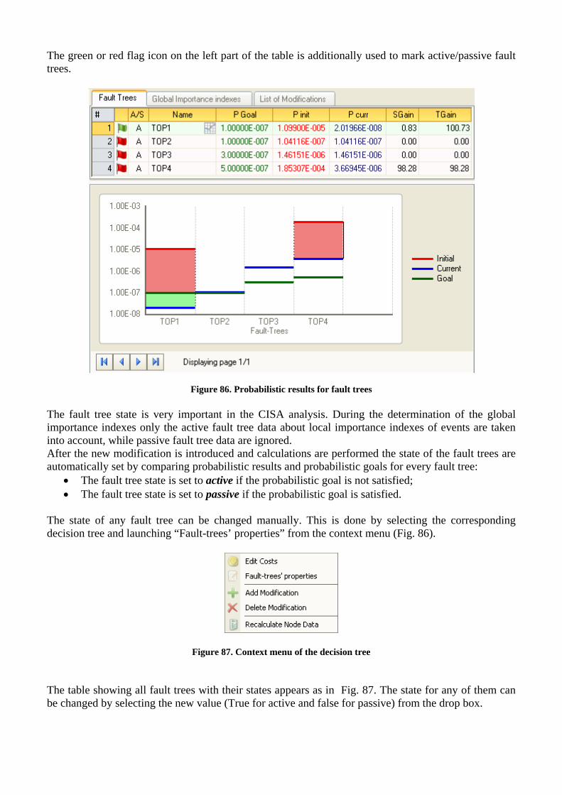
The green or red flag icon on the left part of the table is additionally used to mark active/passive fault trees.

Figure 86. Probabilistic results for fault trees The fault tree state is very important in the CISA analysis. During the determination of the global importance indexes only the active fault tree data about local importance indexes of events are taken into account, while passive fault tree data are ignored. After the new modification is introduced and calculations are performed the state of the fault trees are automatically set by comparing probabilistic results and probabilistic goals for every fault tree:

• The fault tree state is set to active if the probabilistic goal is not satisfied; • The fault tree state is set to passive if the probabilistic goal is satisfied.

The state of any fault tree can be changed manually. This is done by selecting the corresponding decision tree and launching “Fault-trees’ properties” from the context menu (Fig. 86).

Figure 87. Context menu of the decision tree The table showing all fault trees with their states appears as in Fig. 87. The state for any of them can be changed by selecting the new value (True for active and false for passive) from the drop box.

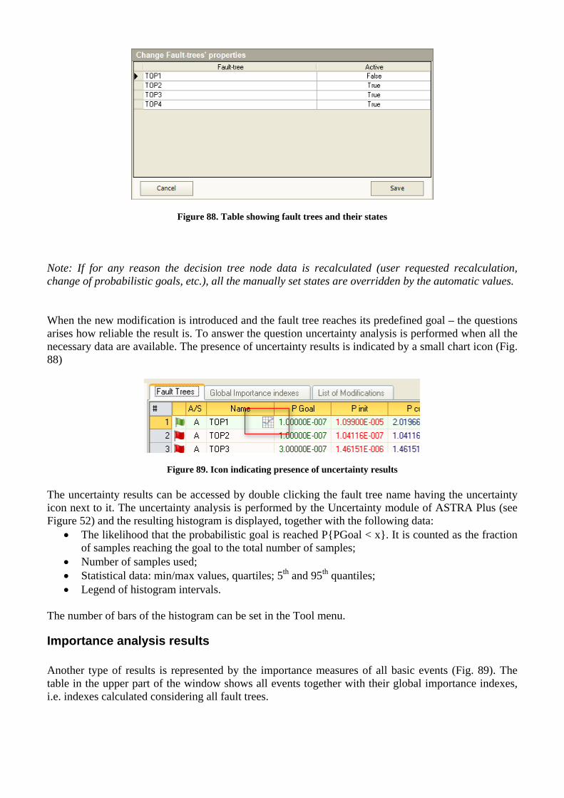
Figure 88. Table showing fault trees and their states Note: If for any reason the decision tree node data is recalculated (user requested recalculation, change of probabilistic goals, etc.), all the manually set states are overridden by the automatic values. When the new modification is introduced and the fault tree reaches its predefined goal – the questions arises how reliable the result is. To answer the question uncertainty analysis is performed when all the necessary data are available. The presence of uncertainty results is indicated by a small chart icon (Fig. 88)

Figure 89. Icon indicating presence of uncertainty results

The uncertainty results can be accessed by double clicking the fault tree name having the uncertainty icon next to it. The uncertainty analysis is performed by the Uncertainty module of ASTRA Plus (see Figure 52) and the resulting histogram is displayed, together with the following data:

• The likelihood that the probabilistic goal is reached P{PGoal < x}. It is counted as the fraction of samples reaching the goal to the total number of samples;

• Number of samples used; • Statistical data: min/max values, quartiles; 5th and 95th quantiles; • Legend of histogram intervals.

The number of bars of the histogram can be set in the Tool menu.

Importance analysis results Another type of results is represented by the importance measures of all basic events (Fig. 89). The table in the upper part of the window shows all events together with their global importance indexes, i.e. indexes calculated considering all fault trees.

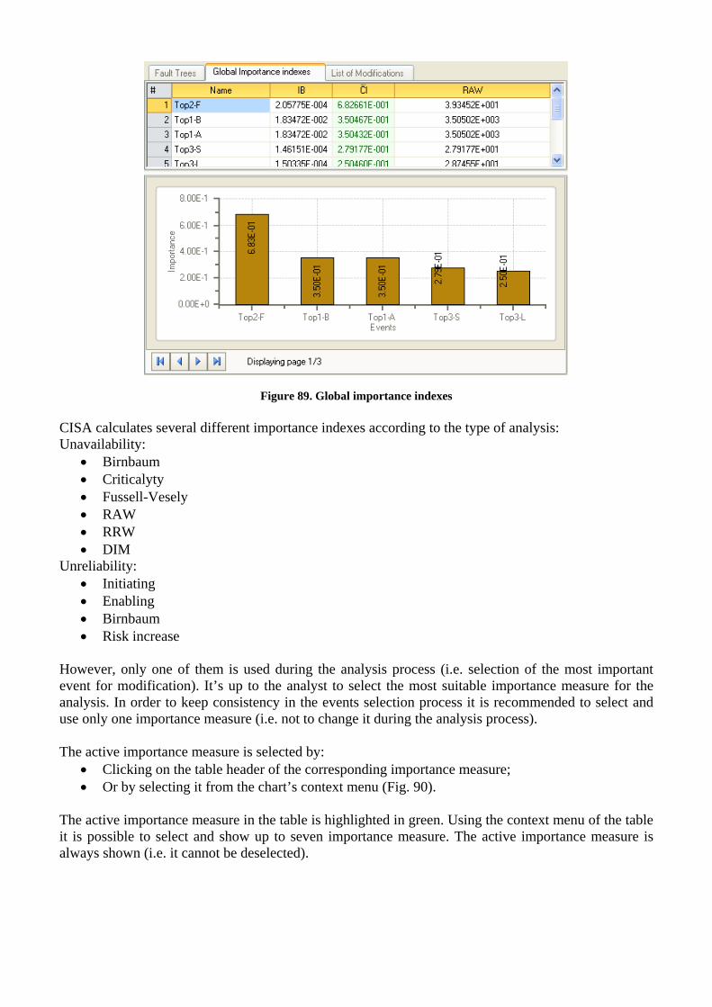
Figure 89. Global importance indexes

CISA calculates several different importance indexes according to the type of analysis: Unavailability:

• Birnbaum • Criticalyty • Fussell-Vesely • RAW • RRW • DIM

Unreliability: • Initiating • Enabling • Birnbaum • Risk increase

However, only one of them is used during the analysis process (i.e. selection of the most important event for modification). It’s up to the analyst to select the most suitable importance measure for the analysis. In order to keep consistency in the events selection process it is recommended to select and use only one importance measure (i.e. not to change it during the analysis process). The active importance measure is selected by:

• Clicking on the table header of the corresponding importance measure; • Or by selecting it from the chart’s context menu (Fig. 90).

The active importance measure in the table is highlighted in green. Using the context menu of the table it is possible to select and show up to seven importance measure. The active importance measure is always shown (i.e. it cannot be deselected).

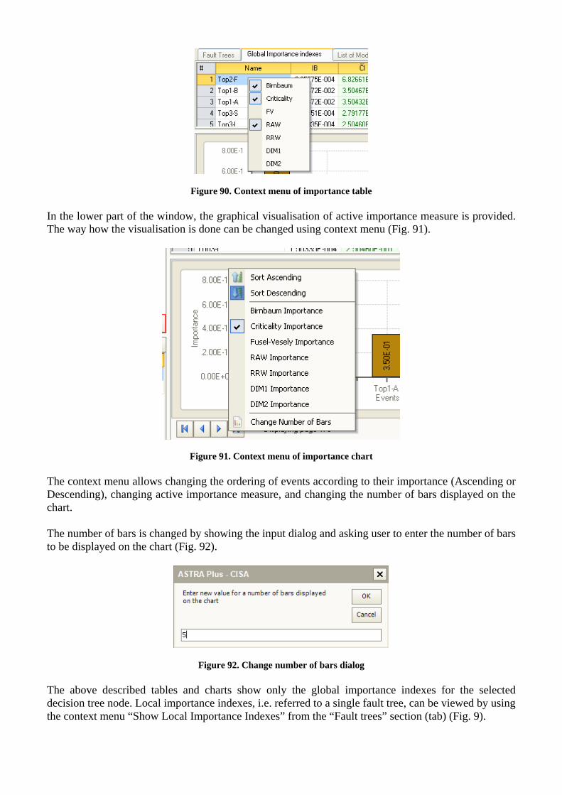
Figure 90. Context menu of importance table In the lower part of the window, the graphical visualisation of active importance measure is provided. The way how the visualisation is done can be changed using context menu (Fig. 91).

Figure 91. Context menu of importance chart The context menu allows changing the ordering of events according to their importance (Ascending or Descending), changing active importance measure, and changing the number of bars displayed on the chart. The number of bars is changed by showing the input dialog and asking user to enter the number of bars to be displayed on the chart (Fig. 92).

Figure 92. Change number of bars dialog The above described tables and charts show only the global importance indexes for the selected decision tree node. Local importance indexes, i.e. referred to a single fault tree, can be viewed by using the context menu “Show Local Importance Indexes” from the “Fault trees” section (tab) (Fig. 9).

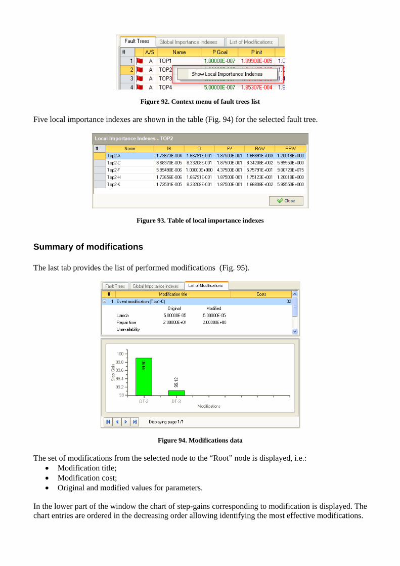
Figure 92. Context menu of fault trees list Five local importance indexes are shown in the table (Fig. 94) for the selected fault tree.

Figure 93. Table of local importance indexes

Summary of modifications The last tab provides the list of performed modifications (Fig. 95).

Figure 94. Modifications data The set of modifications from the selected node to the “Root” node is displayed, i.e.:

• Modification title; • Modification cost; • Original and modified values for parameters.

In the lower part of the window the chart of step-gains corresponding to modification is displayed. The chart entries are ordered in the decreasing order allowing identifying the most effective modifications.

Figure 95. Modifications list (compact) By default all the entries in the table are listed in shorter form by showing only the modification title and the cost. For each record it is possible to expand the entry in order to see modification details.

Ranking of modifications On the left part of the working window, shown in Fig. 69, the list of global ranking of solutions is shown (Fig. 97).

Figure 96. List of top ranked solutions The table displays all solutions available and considered suitable by the analyst, together with their total costs and total gains. If any of the records in the table is selected, the corresponding node in the decision tree representing the selected solution is selected as well. If the selected node in the decision tree represents the solution, then the corresponding row in the solutions ranking table is highlighted.

Managing CISA Project Data

Modifying Probabilistic Goals After the project is created it is still possible to modify probabilistic goals for one or more fault trees. From the menu Project->Probabilistic Goals the dialog showing all project fault trees is launched (Fig. 98).

Figure 97. Input dialog for a new parameter value

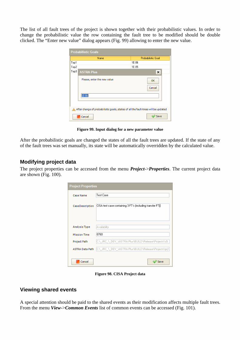
The list of all fault trees of the project is shown together with their probabilistic values. In order to change the probabilistic value the row containing the fault tree to be modified should be double clicked. The “Enter new value” dialog appears (Fig. 99) allowing to enter the new value.

Figure 99. Input dialog for a new parameter value After the probabilistic goals are changed the states of all the fault trees are updated. If the state of any of the fault trees was set manually, its state will be automatically overridden by the calculated value.

Modifying project data The project properties can be accessed from the menu Project->Properties. The current project data are shown (Fig. 100).

Figure 98. CISA Project data

Viewing shared events A special attention should be paid to the shared events as their modification affects multiple fault trees. From the menu View->Common Events list of common events can be accessed (Fig. 101).

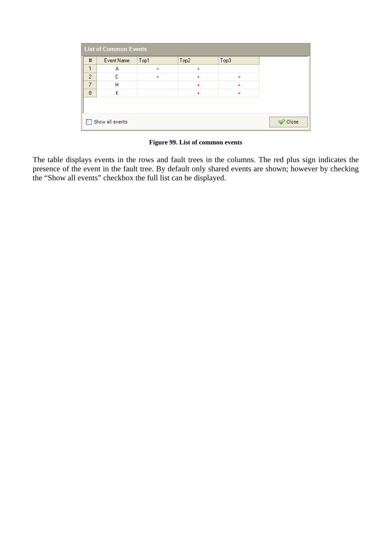
Figure 99. List of common events The table displays events in the rows and fault trees in the columns. The red plus sign indicates the presence of the event in the fault tree. By default only shared events are shown; however by checking the “Show all events” checkbox the full list can be displayed.

ASTRA Plus documentation The following bibliographical references provide details on the theoretical aspects of the methodology implemented in the FTA and CISA modules of ASTRA Plus. [ 1 ] S. Contini, V. Matuzas, ASTRA 3.x: Theoretical Manual, EUR 25052, JRC 67804, ISBN 978-92-79-

22170-5, ISSN 1831-9424, European Union, 2011. [ 2 ] S. Contini, V. Matuzas, ASTRA 3.0 Test Case Report, EUR 24124, JRC 55894, ISBN 978-92-79-14608-

4, ISSN 1018-5593, European Union, 2009. [ 3 ] S. Contini, V. Matuzas, Reduced ZBDD construction algorithms for large fault tree analysis, in: B. Ale, I.

Papazoglou and E. Zio, Editors, Reliability, Risk and Safety: Back to the Future, Rodes, Greece, Taylor & Francis Group, UK, pp. 898–906, 2010.

. [ 4 ] S. Contini, A decomposition method to analyse complex fault trees, in ESREL 2008 Conference on Safety,

Reliability and Risk Analysis: Theory, Methods and Applications, Martorell et al (eds), ISBN 978-0-415-48513-5, 2008

[ 5 ] S. Contini, V. Matuzas, Analysis of fault trees based on functional decomposition, Reliability Engineering

and System Safety, Vol 96, pp 383-390, 2011. [ 6 ] S. Contini, V. Matuzas, Coupling decomposition and truncation for the analysis of complex fault trees, To

appear in Proc. IMechE, Part O: Journal of Risk and Reliability, DOI: 10-1177/1748006x11401495, 2011. [ 7 ] V. Matuzas, S. Contini, Impact of different minimal path set selection methods on the efficiency of fault

tree decomposition, in ESREL 2011 Conference on Advances in Safety, Reliability and Risk Management, Berenguer et al (eds), ISBN 978-0-415-68379-1, 2011.

[ 8 ] Contini S., Fabbri L. and Matuzas V., Concurrent Importance and Sensitivity Analysis Applied to Multiple Fault Trees, JRC IPSC report, EUR 23825 EN, Ispra, 2009. [ 9 ] S. Contini, L. Fabbri, and V. Matuzas, Sensitivity Analysis Applied to Multiple Fault-trees, 4th International CISAP 4 Conference on Safety & Environment in Process Industry, Florence, 2010. [10] S. Contini, L. Fabbri, and V. Matuzas, A novel method to apply Importance and Sensitivity Analysis to

multiple Fault-trees, Journal of Loss Prevention in the Process Industries, 23, pp 574-585, 2010. [11] S. Contini and L. Fabbri, Sensitivity Analysis in support to Design Activities, National Conference on Risk

assessment and Management (Valutazione e Gestione del Rischio negli Insediamenti Civili ed Industriali), Pisa, 2008.

[12] S. Contini, V. Matuzas, Components’ importance measures for initiating and enabling events in fault tree

analysis, EUR 24373, JRC 58492, ISBN 978-92-79-15799-8, ISSN 1018-5593, European Union, 2010. [13] S. Contini, V. Matuzas, New methods to determine the importance measures of initiating and enabling

events in fault tree analysis, Reliability Engineering and System Safety, (2011), doi:10.1016/j.ress.2011.02.001

European Commission EUR 25259 EN – Joint Research Centre – Institute for the Protection and Security of the Citizen Title: Author(s): Sergio Contini, Vaidas Matuzas Luxembourg: Publications Office of the European Union 2012 – 68 pp. – 21 x 29.7 cm EUR – Scientific and Technical Research series – ISSN 1831-9424 (online), ISSN 1018-5593 (print)ISBN 978-92-79-23390-6 doi:10.2788/17628 Abstract This report describes the user interface and the main commands to perform system dependability analysis by means of ASTRA Plus. This package implements the analysis methods developed at the Institute for the Protection and Security of the Citizen from mid-2008. ASTRA Plus is composed of the Fault Tree Analysis (FTA) module and of the Concurrent Importance and Sensitivity Analysis (CISA) module. The FTA module contains three different methods for solving a fault tree; all are based on the state of the art approach of Binary Decision Diagrams (BDD). These three methods allow the user to analyse fault tree of increasing complexity (i.e. increasing number of basic events and gates). In particular the third method, which is based on functional decomposition, allow performing the analysis of fault trees of very high complexity. The CISA module is based on a new methodology for system design improvement. The key operation is the calculation of Global Importance Measures of basic events considering all system fault trees. This allows to identify the weakest part of the system with reference to all top-events. Then the on-line sensitivity analysis, allows the user to rapidly identify the set of suitable design improvements from which the best cost-effective one can be selected.

How to obtain EU publications

Our priced publications are available from EU Bookshop (http://bookshop.europa.eu), where you can place an order with the sales agent of your choice. The Publications Office has a worldwide network of sales agents. You can obtain their contact details by sending a fax to (352) 29 29-42758.

67

The mission of the JRC is to provide customer-driven scientific and technical support for the conception, development, implementation and monitoring of EU policies. As a service of the European Commission, the JRC functions as a reference centre of science and technology for the Union. Close to the policy-making process, it serves the common interest of the Member States, while being independent of special interests, whether private or national.

LB

-NA

-25259-EN-N