3rd HEPEX workshop (Stresa, Italy, 27-29th June 2007)

BOOK of ABSTRACTS

Editors: J. Thielen, J. Bartholmes and J. Schaake

EUR 22861 EN - 2007

The mission of the Institute for Environment and Sustainability is to provide scientific-technical support to the European Union’s Policies for the protection and sustainable development of the European and global environment. European Commission Joint Research Centre Institute for Environment and Sustainability Contact information Address: Via E. Fermi, TP261, 21020 Ispra (VA), Italy E-mail: jutta.thielen@jrc.it Tel.: + 39 0332 785455 Fax: + 39 0332 786653 http://ies.jrc.ec.europa.eu http://www.jrc.ec.europa.eu Legal Notice Neither the European Commission nor any person acting on behalf of the Commission is responsible for the use which might be made of this publication. A great deal of additional information on the European Union is available on the Internet. It can be accessed through the Europa server http://europa.eu/ JRC37599 EUR 22861EN ISSN 1018-5593 Luxembourg: Office for Official Publications of the European Communities © European Communities, 2007 Reproduction is authorised provided the source is acknowledged Printed in Italy

European Commission EUR 22861EN – Joint Research Centre – Institute for Environment and Sustainability Title: 3rd HEPEX workshop, Book of abstracts Editors: J. Thielen, J. Bartholmes and J. Schaake Luxembourg: Office for Official Publications of the European Communities 2007 EUR – Scientific and Technical Research series – ISSN 1018-5593 Abstract This Book of Abstracts is a collection of abstracts presented during the 3rd HEPEX workshop

held at Stresa from 27th to 29th June 2007.

Specific sessions of the workshop address the following subjects:

• HEPEX testbeds, datasets and forecast tools

• Ensemble weather and climate forecast applications

• Hydrologic ensemble processing

• Best practice for analyzing and visualizing uncertainty

• User perspectives

The 3rd HEPEX workshop has been organised and coordinated jointly by HEPEX, the

Hydrologic Ensemble Prediction Experiment and the European Commission, Joint Research

Center, Ispra, Italy

iv

v

Scope of the workshop

The first HEPEX workshop was held in Reading, England in the spring of 2004. During this workshop scientific questions were formulated that, once addressed, should help produce valuable hydrological ensemble prediction to serve users’ needs. The second workshop was held in Boulder, Colorado in the summer of 2005. Its aim was to set up a series of coordinated test-bed demonstration projects as a method for answering these questions. The third workshop will report on the progress of the testbeds and is meant to be interdisciplinary, fostering communication between research meteorologists, hydrologists and end users. Its aim is to further help the hydrologic community to develop hydrologic ensemble prediction systems that can be used with confidence by emergency and water resource managers. Specific sessions of the workshop address the following subjects: • HEPEX testbeds, datasets and forecast tools • Ensemble weather and climate forecast applications • Hydrologic ensemble processing • Best practice for analyzing and visualizing uncertainty • User perspectives The 3rd HEPEX workshop has been organised and coordinated jointly by HEPEX, the Hydrologic Ensemble Prediction Experiment and the European Commission, Joint Research Center, Ispra, Italy Workshop organising committee: John Schaake (NOAA) Jutta Thielen (EC JRC) Roberto Buizza (ECMWF) Robert Hartmann (NOAA)

vi

vii

Acknowledgements The organisers would like to thank all participants that contributed with abstracts to this book to make it a successful collection of good ideas on ensemble predictions in hydrology. Special thanks also goes to Mrs Rizzi who set up the registration site and who takes care of the logistics of this workshop. Kristie Franz is thanked for updating the HEPEX webpage with the latest workshop details.

Participants of the 3rd HEPEX workshop held in Stresa on 27-29th June 2007

viii

ix

Table of Contents (in alphabetical order according to authors)

A-B ......................................................................................................................... 13 Assessing operational forecasting skill of EFAS by J. Bartholmes, J. Thielen, S. Gentilini .........................................................................................................................13 Ensemble uncertainty representation in satellite QPE by T. Bellerby and J. Sun.........16 Bias correction methods and evaluation of an ensemble based hydrological forecasting system for the Upper Danube catchment by Bogner, K., Thielen, J. and De Roo, A.P.J.21 Meteorological input for hydrological ensemble forecast by I. Bonta ..........................23 The new ECMWF Variable Resolution Ensemble Prediction System by R. Buizza ......30

C-D ......................................................................................................................... 34 Application of meteorological ensemles for Danube flood forecasting and warning by A. Csík, G. Bálint*, P.Bartha and B. Gauzer................................................................34 How should we compare hydrological models by R. T. Clarke.....................................38 A meteo-hydrological prediction system based on a multi-model approach for ensemble precipitation forecasting by T. Diomede, S. Davolio, C. Marsigli, M. M. Miglietta, A. Morgillo and A. Moscatello ......................................................................43 Discharge ensemble forecasts based on the COSMO-LEPS quantitative precipitation by T. Diomede, C. Marisgli, A. Montani and T. Paccagnella .......................................48

E-F.......................................................................................................................... 52 Status of the Great Lakes Testbed project by V. Fortin and A. Pietroniro....................52 Short-term streamflow prediction for a small midwestern watershed by K. J. Franz, W. A. Gallus, M. Baker, K.A. Jungbluth and W. S. Lincoln ................................................53

G-H......................................................................................................................... 54 Experimental Ensemble Forecasts of Precipitation based on a Convection-Resolving Model by C. Gebhardt, S.Theis, P. Krahe, and V. Renner ............................................54 Hydrological ensemble prediction systems: the 1966 century flood experiment by G. Grossi, B. Bacchi, R. Buizza and R. Ranzi.....................................................................58 Moving toward operational hydrologic ensemble forecasts by R.K. Hartman .............63 Addressing parameter uncertainty in regional forecast basins using similarity indices by T. Hogue, S. Lopez, K. Franz and J. Barco...............................................................64 Ensemble streamflow forecasting with the coupled GFS-NOAH modeling system by D. Hou, K. Mitchell, Z. Toth, D. Lohmann and H. Wei ......................................................65 Hydroelectric Operations - Ensemble Optimization Procedures (EOP) by C. D. D. Howard ..........................................................................................................................69

K-L.......................................................................................................................... 70 Evaluation of the medium-range European flood forecasts for the March-April 2006 flood in the Morava river by M. Kalas, M.H. Ramos and J. Thielen.............................70 Improving precipitation generation for seasonal hydrological prediction by L. Luo and E.F. Wood ......................................................................................................................71

x

M-N......................................................................................................................... 72 Matching time-steps and updating cycle of meteorological PQPF’s to fit hydrological needs and to produce ensemble discharge forecasts by R. Marty, A. Djerboua, I. Zin and Ch. Obled ................................................................................................................72 Probabilistic Streamflow forecast in norway by M. Morawietz, T. Skaugen and E. Langsholt........................................................................................................................73 Hydrological climate change impact assessment over the Blue Nile using ensemble statistical downscaling by R. Nawaz, T. Belleby and M. Elshamy ................................77 The groundwater recharge and meteorological data by O. Nitcheva ...........................82

O-P ......................................................................................................................... 83 Analog based post-processing of meteorological forecasts for basinwide PQPF’s: principles and operational aspects by C. Obled, A. Djerboua, R. Marty and I. Zin .....83 A User Guide to the Risk and uncertainty decision tree by F. Pappenberger, K. Beven, H. Harvey, D. Leedal, and J. Hall .................................................................................84 Comparison of catchment and grid based model evaluation of precipitation for hydrological applications on the example of the July/August 2002 flood in the Danube by F. Pappenberger and R. Buizza ................................................................................88 An ensemble hydrological forecasting system for the Laurentian Great Lales by A. Pietroniro, V. Fortin*, N. Kouwen, I. Doré, C. Neal, K. Legault, D. Nsengiyumva, E. Klyszejko, R. Turcotte, B. Davison, D. Verseghy, E.D. Soulis, R Caldwell, N. Evora and P. Pellerin ...............................................................................................................93

Q-R......................................................................................................................... 97 EFAS EPS based forecasts: in-depth case study analyses and statistical evaluation of summer 2005 and sprink 2006 flood forecasts by M.H. Ramos, J. Thielen and J. Bartholmes .....................................................................................................................97 The Map D-Phase operations period (DOP) by M. W. Rotach and M. Arpagaus ......101

S-T........................................................................................................................ 102 Assessment of bias removal for deterministic medium-range weather forecasts in the Po river basin, Italy, Europe by Salamon, P., and Thielen, J......................................102 Statistical re-scaling and downscaling testbed project: status reportby J. Schaake ...103 Weather and Society- integrated studies (WAS IS): is the WAS IS initiative relevant to HEPEX? by S. Theis ....................................................................................................109 European flood Alert System: Early flood warning based on ensemble prediction system products by Thielen J., J. Bartholmes, M.H. Ramos, M. Kalas , and A.de Roo111 Reconciling hydrological physically based models and data driven models in terms of predictive probability by E. Todini, G. Coccia and C. Mazzetti..................................116 Improving the NASA land information system in support of NOAA NWSRFS ensemble hydrologic predictions by D. Toll, B. Cosgrove, P. Houser, J. Dong and L.G. de Goncalves.....................................................................................................................120 Short- and Long-term flow forecasting in Rio Grande Water shed by C.E.M. Tucci, W. Collischonn, R.T. Clarke, A. R. Paz and D. Allasia.....................................................124

U-V-W................................................................................................................... 129 Rijnland case study: anticipatory control of a lowlying regional water system by S. J. Van Andel, A. Lobbrecht and R. Price.........................................................................129 Downscaling global medium range meteorological predictions for flood prediction by N. Voisin, A.W. Wood and D.P. Lettenmaier ...............................................................134

xi

Recent advances in data assimilation and postprocessing in operational ensemble flood forecasting by A. Weerts, P. Reggiani and M. Werner.......................................135 Multiple ensemble forecasts in the operational forecasting system for the Rhine basin in Switzerland by M. Werner, M.v.Dijk, T. Buergli and S. Vogt................................136 Correcting errors in streamflow forecast ensemble mean and spread by A. Wood ...137 Using CPC seasonal climate outlooks for ensemble hydrologic prediction by A. Wood, X. Zeng and D. P. Lettenmaier ....................................................................................138

X-Y-Z .................................................................................................................... 139 Performance of the European Flood Alert System during the Spring 2006 floods in the Cz Elbe by J. Younis, M.H. Ramos and J. Thielen.......................................................139

xii

13

A-B

Assessing operational forecasting skill of EFAS by J. Bartholmes, J. Thielen, S. Gentilini

Assessing operational forecasting skill of EFAS Jens Bartholmes1*, Jutta Thielen1, Simone Gentilini1

1 EC, Joint Research Centre, Institute for Environment and Sustainability (IES), Via E. Fermi 1, 21020 Ispra (Va) * Corresponding author: Jens Bartholmes Tel.: 0039-0332-786711 E-mail: jens.bartholmes@jrc.it Abstract The European Flood Alert System (EFAS) is now producing probabilistic hydrological forecasts in pre-operational mode for over 2 years at the European Commission Joint Research Centre (JRC). EFAS is aiming at increasing preparedness for floods in trans-national European river basins by providing medium-range deterministic and probabilistic flood forecasting information between 3 to10 days in advance. It is providing EFAS information reports regarding forecasted riverine flood events to the collaborating national hydro-meteorological services. Memoranda of Understanding (MoU) for receiving these forecasts have been established for ca. 80% of the area of all European trans-national river basins. In this work 2 years of existing operational hydrological forecasts are being assessed statistically and skill of EFAS is analysed in several ways. The goal is to show where the strengths of such a large scale system lie but also where the limits of predictability and limits of skill scores in this context are. Introduction The scope of EFAS is to raise preparedness previous to a possibly upcoming flood event in order to leave more time for the organization of countering measures and mitigation. Furthermore, EFAS gives a, hitherto not available, unified overview of flood forecasts over the whole of Europe that uses the same warning nomenclature for all river basins thus facilitating a trans-national overview. EAFS is making use of deterministic weather forecasts of the European Centre for Medium-Range Weather Forecasts (ECMWF) and of the German national weather service (DWD). The probabilistic forecasts (51 members) are based on the Ensemble Prediction System (EPS) of ECMWF. The objective of this work is to assess the skill of this specific operational hydrological forecasting system, which to this extend (to the knowledge of the author) has not been reported in literature before. For this purpose 2 years of pre-operational EFAS medium-range deterministic and probabilistic flood forecasts with up to 10 days in advance were analysed statistically for the whole of Europe. Because of (distributed) nature of EFAS this data intensive skill assessment cannot make use of the traditional hydrological approach as it cannot make use of observed discharges, in fact it is using a proxy (hydrologic simulation with observed meteo data). Most suitable skill scores and visualizations are reviewed and pros and cons are analysed. This skill assessment is looking at the past performance but is also designed to improve the future performance of such a system by making it possible to incorporate the past experience into the current forecast. By making the past performance easily accessible at each pixel the forecaster can better evaluate the probability of a current forecast. This is especially useful as the study showed that the meteorological assumed equi-probability of forecast members does (in the case of EFAS) not linearly translate into the hydrological probabilistic forecasts and that there are biases.

14

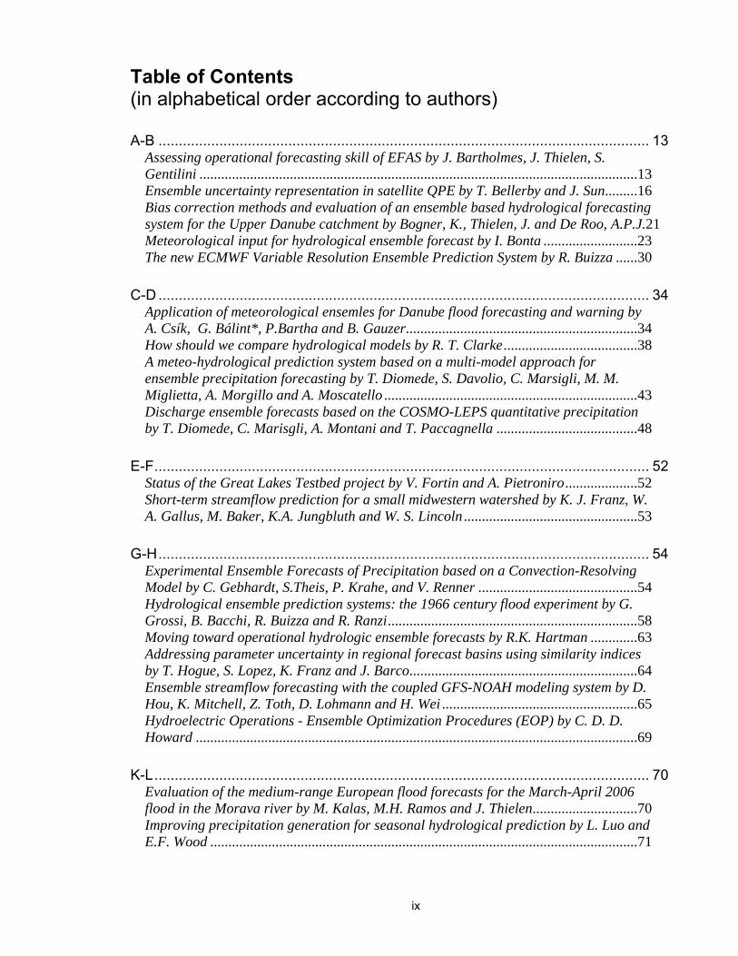
Some Results Among other results the study showed that the use of the “persistency” criterion1 is very efficient in lowering the number of false alerts and thus increasing the skill of the issued forecast. Figure 1 shows the influence of persistency on the Brier Skill score (BSS). Without persistency the mean of the BSS is close to 0.0 (no skill) or even far below. When regarding persistency the picture changes and BSS reach very high values. When at least 20 EPS are persistent the BSS of deterministic and probabilistic forecasts is quite the same.

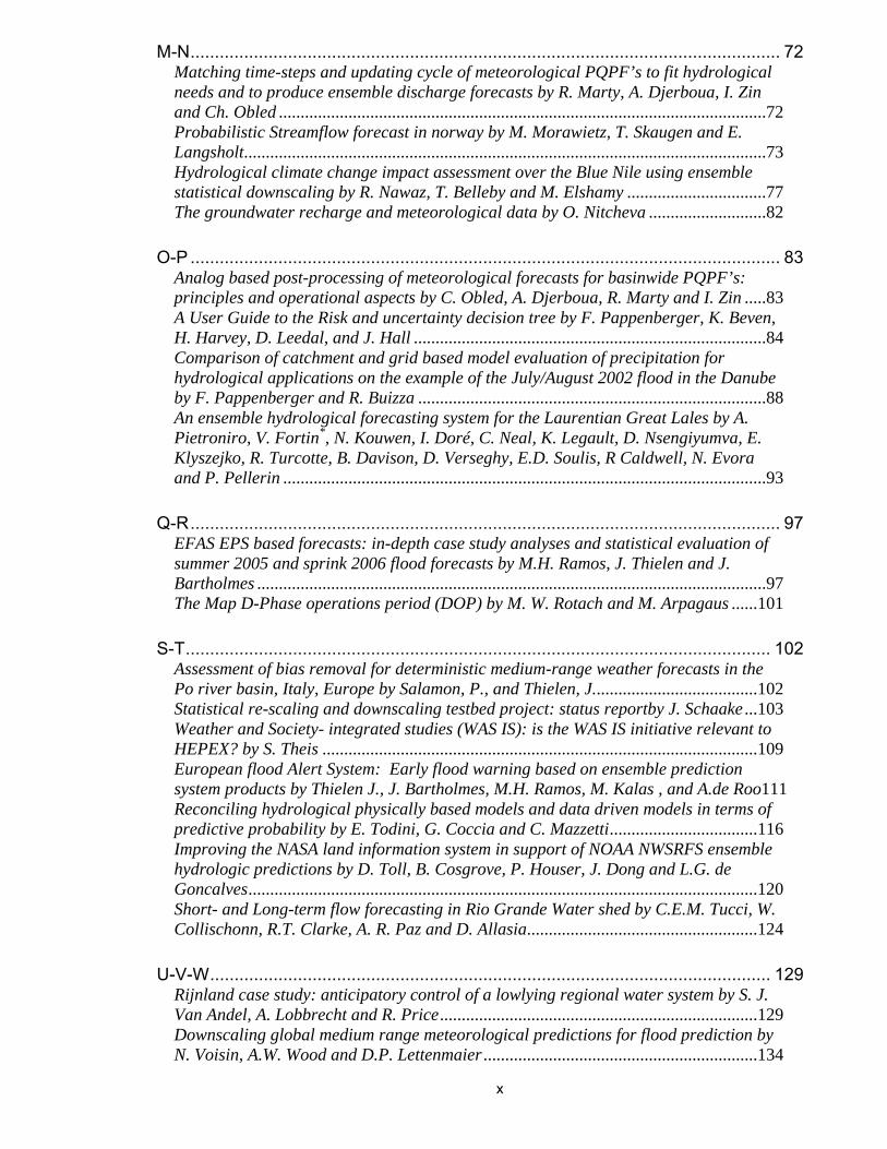
Figure 1: Positive influence of the persistency criterion on the skill expressed as Brier Skill score (BSS) (≤0 no skill, max=1) When using the Hanssen-Kuipers (HKTSS) score the picture changes as i) the skill score is decreasing with leadtime (a more intuitive result) an ii) the skill expressed as HKTSS of EPS is always higher than the skill of the deterministic forecasts.

Figure 2: Hanssen-Kuipers skill score (HKTSS) for deterministic forecasts with persistency and probabilistic forecasts with at least 5 persistant EPS. Furthermore, the numerical analysis showed that the observed frequencies of hits did not match the theoretically expected frequency that should be proportional to the forecasted probability of the EPS. As can be seen in the reliability diagrams in Figure 2 the EFAS EPS forecasts tend to “over-forecast”. Even more interesting is, for example, the fact that in the

1 Persistency: the forecasted discharge in a pixel exceeded the same EFAS alert threshold in two consecutive forecast dates (with at least the same number of EPS members).

15

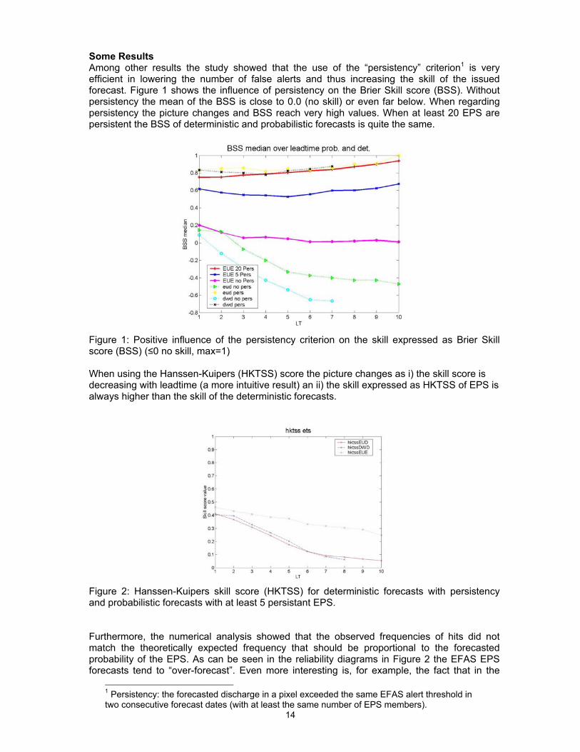
case that the previous forecast had at least 20 EPS exceeding the EFAS High threshold (Fig. 2 right), the probability (around 30%) to have a hit (with leadtime 3 days) is almost not changing if the present forecast is between 1 and 25 EPS > threshold.

Figure 3: Reliability diagram of EPS without persistency (left) and with 20 persistent EPS (right). For points on the diagonal the observed frequency corresponds to the forecasted probability. Conclusions The present work showed several interesting and counterintuitive results, and these findings will be incorporated in the pre-operational EFAS system to improve its performance. One of the critical points of this analysis was that 2 years of data was just enough to get some reasonable results and as the events that were analysed are to be classified as rare (aprox. 1-2 year return period) not all river pixels had a sufficient amount of events to fill all the four fields of the contingency table. Further work is ongoing regarding the best choice of skill factors that, as was alluded to in the results section, can give quite opposite impression concerning the skill of a system. Therefore, it is necessary to consider also the absolute values and numbers of the input data when expressing the skill through some compressed skill factor.

16

Ensemble uncertainty representation in satellite QPE by T. Bellerby and J. Sun

ENSEMBLE UNCERTAINTY REPRESENTATION IN SATELLITE QPE Tim Bellerby1* and Jizhong Sun2 1 Department of Geography, University of Hull, UK. 2 Department of Physics, University of Hull, UK. * Corresponding author: Tim Bellerby, Geography Dept. University of Hull, Hull, HU67RX,UK. (44) 1482 465385. Email: t.j.bellerby@hull.ac.uk Abstract This paper demonstrates that ensemble representations may be extended beyond their traditional application in Quantitative Precipitation Forecasting (QPF) to represent the uncertainty in Quantitative Precipitation Estimation (QPE). The methodologies reviewed have been specifically developed for high-resolution multi-sensor satellite rainfall retrievals (which contain a high degree of uncertainty and complex error structures) but are potentially applicable to a wider range of QPE technologies. 1. Introduction Many large river basins are poorly instrumented and there is a continuing interest in the use of satellite precipitation estimates to drive hydrological models for these catchments. However, satellite estimates contain both a considerable degree of uncertainty and complex and highly skewed error distributions. A general representation of the uncertainty in a point satellite rainfall retrieval is given by the conditional probability of a given rainfall rate, R(x,t), at location x and time t, being associated with satellite data S(x,t): p(R(x,t)|S(x,t)). This representation is sufficient for applications such as meteorological model data assimilation. However, for hydrological applications it must be noted that these uncertainties are both spatially and temporally correlated and that the field of conditional expected values, E[R(x,t)|S(x,t)] is unlikely to display a realistic spatiotemporal structure or to effectively reproduce point rainfall frequency distributions. To construct an effective satellite-driven hydrological model and to assess the impact of precipitation-related uncertainty on runoff and other hydrological variables, it is necessary to generate an ensemble precipitation product, each element of which displays a predetermined pattern of spatial and temporal variability while remaining consistent with the original satellite data. Ensemble uncertainty models meeting these criteria have recently been published by several groups (Bellerby and Sun, 2005; Hossain and Anognostou, 2006; Teo, 2006). An ensemble satellite-rainfall product is generated in two stages. In the first stage, the cdf p(R(x,t) |S(x,t)) is derived for each point precipitation retrieval. If S(x,t) consists of a single scalar variable then a simple curve-fitting approach may be used to determine the cdf. If S(x,t) is a more general multi-dimensional input vector the problem becomes more complex. Artificial Neural Networks (ANN) represent one approach to address this more general case. Once the cdfs have been determined, the spatiotemporal covariance structure of the retrieval uncertainty must be modelled. This covariance and cdf models may then be combined to parameterise a stochastic rainfall generator. The generator creates the required ensemble of precipitation fields. 2. Methodology 2.1 Deriving CDFs with respect to a scalar predictor variable Bellerby and Sun (2005) describe the development of an ensemble precipitation product conditioned on a single satellite input: infrared (IR) brightness temperature from Geostationary Operational Environmental Satellite (GOES) band 4 (10.7μm) infrared imagery. The uncertainty model was calibrated over Florida against Tropical Rainfall Measuring Mission (TRMM) 2B31 combined rain-profiling algorithm data for August and September 1998 and

17

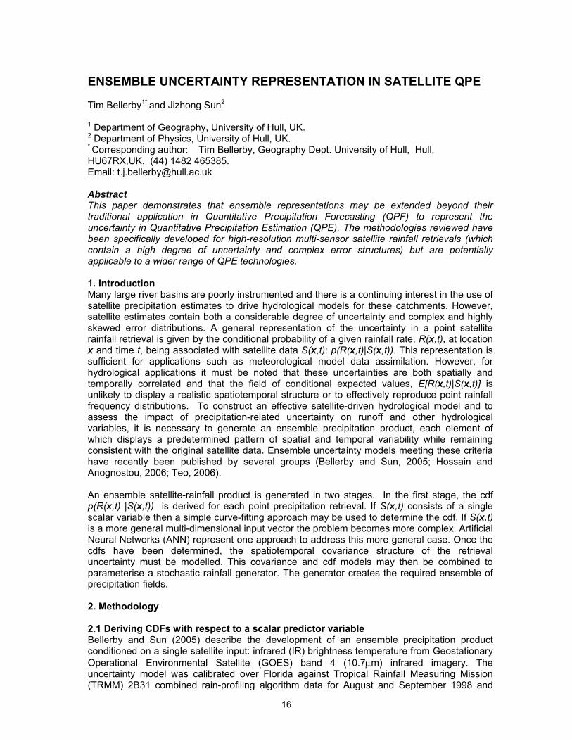
validated against the ground-based precipitation radar at Melbourne, Florida (TRMM ground-validation product 2A53). All of these measurements were aggregated to a common 0.1-degree spatial resolution and 15 minute temporal resolution. The TRMM precipitation data were divided into categories, each category corresponding to a ten-degree range of coincident IR brightness temperatures. The distribution function for rainfall rates in each category was then determined. (Fig. 1).

0

5

10

15

20

25

30

0 0.2 0.4 0.6 0.8 1

Cumulative Probability

Rai

nfal

l Rat

e, m

mh-1

205-215K215-225K225-235K245-255K

A two parameter gamma distribution was fitted to the distribution for each category using maximum likelihood analysis. The two parameters to each gamma distribution, together with the probability of zero rainfall, were then fitted to empirical functions of brightness temperature to create a conditional distribution function that changed continuously with brightness temperature. 2.2 Modelling the spatiotemporal structure of retrieval uncertainty Once p(R(x,t)|S(x,t)) has been determined for a given calibration domain, an ensemble of possible realisations of the precipitation field may be stochastically generated using:

⎩⎨⎧

<≥

=−

)),(;0()),((0)),(;0()),(()),());,(((

),(1

tSFtzNtSFtzNtStzNF

tRi

iii xx

xxxxx (1)

where F(R|S(x,t))=p(R(x,t)≤R|S(x,t)) is the cumulative conditional cdf, N(z) is the cumulative standard normal distribution function and zi(x,t), i=1,2,..N, are a set of standard normal random fields that display the same spatiotemporal structure as the uncertainty in the precipitation field. An exemplar for the uncertainty fields may be derived from calibration data, R*(x,t) using:

⎩⎨⎧

=>

=−

0),(0),())),();,(((

),(*

**1*

tRifUndefinedtRiftStRFN

tzxxxx

x (2)

Since it is impossible to assign a unique value to zero-rainfall values, the covariance structure of z*(x,t) must be calculated using data from raining points only. Bellerby and Sun (2005) used an isotropic, second order stationary model for the

spatiotemporal covariance function22

),( tbxaetC δδδδ −−=x , where a and b are empirically determined constants. A three-dimensional Turning Bands Method (Tompson et al., 1989) using 200 lines randomly distributed on the unit sphere was used to simulate 500 random fields , zi(x,t), in two spatial dimensions and one temporal dimension

Figure 1. (From Bellerby and Sun, 2005). Cumulative frequency histograms of rainfall rates of raining points from TRMM data categorised according to coincident GOES Band 4 brightness

temperatures.

18

2.3 Deriving CDFs with respect to a general input vector The methodology described in 2.1 may apply to any scalar predictor of precipitation. This may either be a single satellite cloud index, such as IR brightness temperature, or it may be a precipitation estimate derived from a combination of satellite data, leading to an error-modelling approach to ensemble generation (Hossain and Anognostou, 2006). In each of these cases, the cdf is uniquely characterised by the conditional expected rainfall rate. However, it is possible to envisage cases where two separate meteorological conditions, distinguished by different patterns of satellite input data, yield the same expected rainfall rate while being associated with very different distributions of retrieval error. To most quantify the retrieval uncertainty in complex satellite-precipitation algorithms effectively, it is necessary to model the cdf as a function of multidimensional input data rather than of a single scalar predictor variable. Neural networks provide a flexible tool for non-linear regression and form the basis of a number of multiplatform satellite rainfall algorithms. These techniques may be extended to derive conditional distributions as opposed to simply deriving conditional expected values. Bellerby (in review) describes the development of such a network architecture, based on a histogram representation of the cdf, p(R(x,t)∈Bi|S(x,t)) using N bins, Bi, where:

{ }{ }

{ } NiNi

i

RRRRRRR

RRB

N

iin

=<<=

⎪⎩

⎪⎨

⎧

<≤<=

= + 10

||

0|

1 (3)

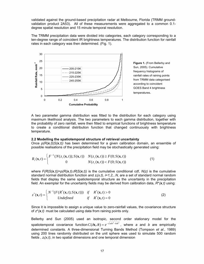
A histogram representation of the cdf does not provide any information on the shape of the conditional distribution for high rainfall rates; these are all grouped into a single bin. However, any characterisation of the high end of the conditional distribution would by definition be an extrapolation and Bellerby and Sun (2005) suggest that extending an estimated cdf beyond the range of rainfall rates represented in the calibration dataset is unlikely to be successful. The high end of the conditional distribution may be modelled using the climatological distribution of rainfall rates falling in the highest bin. 3. Results The technique of Bellerby and Sun (2005) was validated against 2A53 ground radar data as follows: 1. For each pixel location and time, exceedence probabilities for rainfall rates 0, 5, 10 and 20 mmh-1 were estimated from the 500 simulated scenarios. 2. The estimated exceedence probabilities were divided into categories, each corresponding to a 1% probability range. 3. Coincident radar data were categorised according to results of step 2 and exceedence probabilities were computed for the radar rainfall rates in each category This procedure results in pairs of simulated and observed exceedence probabilities that should match each other if the technique was effectively determining the uncertainty in the precipitation field.

19

Figure 2 (from Bellerby and Sun (2005)) Simulated exceedence probabilities

computed using the ensemble satellite product plotted against observed exceedence probabilities computed using coincident ground radar data for points with the given

simulated exceedence probability.

Figure 3. (Adapted from Bellerby and Sun (2005)) A comparison of the structural characteristics of an arbitrary component of the ensemble product to those displayed by coincident ground radar data. In each case, the error bars on the simulated data indicate variability across the ensemble (ensemble 10% and 90% percentiles). (a) Frequency distribution of storm durations. (b) Mean rainfall while raining as a function of spatial resolution.

10mmh-1

0

0.02

0.04

0.06

0 0.02 0.04 0.06

Simulated Probability

Coi

ncid

ent O

bser

ved

Prob

abili

ty

0mmh-1

0.2

0.4

0.6

0.2 0.4 0.6

Coi

ncid

ent O

bser

verv

ed

Prob

abili

ty

5mmh-1

0

0.1

0.2

0.3

0 0.1 0.2 0.3

20mmh-1

0

0.005

0.01

0.015

0 0.005 0.01 0.015

Simulated Probability

(a)

0.001

0.01

0.1

1

0 50 100 150

Storm Duration, min

Nor

mal

ised

Fre

quen

cy Observed

Simulated

(b)

0

1

2

3

4

0 0.2 0.4 0.6 0.8 1

Spatial Scale, degrees

Mea

n R

ainf

all w

hen

Rai

ning

, m

mh

-1

Observed

Simulated

20

The spatiotemporal structures of the simulated precipitation fields were compared to ground radar data using two statistics considered relevant to the utility of the retrieval algorithm in a hydrological modelling context. These were the frequency distribution of storm durations (Figure 3a) and the mean rainfall rate while raining as a function of spatial scale (Figure 3b). 4. Conclusions A number of recent papers have demonstrated that ensemble precipitation products may be generated from satellite rainfall algorithms. The mathematics of the ensemble modelling are not specific to satellite data and could be used to model uncertainty in other forms of QPE. References

- Bellerby, T. in review. Satellite rainfall uncertainty estimation using an artificial neural network. Journal of Hydrometeorology.

- Bellerby, T. and J Sun, 2005. Probabilistic and ensemble representations of the uncertainty in an IR/microwave satellite precipitation product. Journal of Hydrometeorology, 6, pp. 1032-1044

- Hossain, F. and E. N. Anognostou, 2006. A two-dimensional satellite rainfall error model. IEEE Transactions on Geoscience and Remote Sensing, 44, pp. 1511- 1521.

- Teo, C.K., 2006. Application of satellite-based rainfall estimates to crop yield forecasting in Africa. Unpublished Ph.D. Thesis, University of Reading. UK.

- Tompson, A.F.B, R. Ababou and L.W. Gelhar, 1989. Implementation of the three dimensional Turning Bands random field generator, Water Resources Research, 25(10), pp. 2227-2243.

21

Bias correction methods and evaluation of an ensemble based hydrological forecasting system for the Upper Danube catchment by Bogner, K., Thielen, J. and De Roo, A.P.J.

Bias correction methods and evaluation of an ensemble based hydrological forecasting system for the Upper Danube catchment Bogner, K., Thielen, J. and De Roo, A.P.J. European Commission Joint Research Centre, Institute for Environment and Sustainability, Ispra (VA) email: konrad.bogner@jrc.it

Abstract Within the EU Project PREVIEW (Prevention, Information and Early Warning) various weather forecast products from ECMWF, DWD, ARPA-SIM and IMK will be compared. Based on this system of meteorological forecasts ensembles of discharge series have been generated for the hydrological year 2002 for the Danube catchment upstream Bratislava. The main objective is to get a probabilistic streamflow forecast by the use of different Ensemble Prediction Systems (EPS) and to derive performance criteria not only for flood events (like the flood event of August 2002), but also to evaluate the technical quality of the different forecasting systems continuously within the year. Hydrological models used for ensemble streamflow prediction often have simulation biases that degrade forecast quality and limit the operational usefulness of the forecasts. Therefore different methods of bias correction have been applied and tested for adjusting the ensemble traces using a transformation derived with simulated and observed flows from the Year 2002: 1. Wavelet transformation (breaking the data into a set of scaled and translated versions of a wavelet function) + Bayesian Time Series Analysis (dynamic linear model for each scale) • Magnitude and scale of model error show time dependences, which requires localization in time and consideration of the time-scale over which error is manifest. This could be done by Wavelet transformation breaking the observed and simulated runoff series into a set of scaled and translated versions of a wavelet function (Lane, 2007). On each set a dynamic linear model (DLM), also known as linear state space model, is applied (West and Harrison, 1997). 2. Kernel based machine learning methods • Most recently the application of data-driven models based on statistical learning methodology has attracted attention in the field of hydrological engineering (see Yu, Chen, and Chang, 2006). Kernel based learning methods use an implicit mapping of input data into high dimensional feature space defined by a kernel function (e.g. the Gaussian radial basis function). In this presentation two kernel based methods will be tested: 1. the Support Vector Machine (SVM) and 2. the Relevance Vector Machine (RVM), which is a probabilistic sparse kernel and adopts an Bayesian approach for learning. In order to combine the predictive distributions from different forecast systems the method of Bayesian Model Averaging (BMA) will be applied (Raftery, Balabdaoui, and Polakowski, 2005). The BMA predictive probability density function (PDF) of any future weather and/or hydrological quantity of interest is a weighted average of PDFs centered on the bias-corrected forecast from a set of different models. The weights assigned to each model are posterior probabilities and reflect that model’s contribution to the forecasting skill over a training period. Weights must be applied to the ensemble members, which can be equal if all members are assumed equally likely to occur, or unequal if not. For the modelling of the probabilities in the tails of the distribution, outside the ensemble, extreme value distributions, such as the Generalized Pareto distribution, could be fitted. Finally the quality of probabilistic forecasts issued when using the different bias-correction methods is evaluated and first results will be shown

References

22

- S. N. Lane. Assessment of rainfall-runoff models based upon wavelet analysis. Hydrological Processes, 21(5):586–607, 2007.

- T. Raftery, A.E.and Gneiting, F. Balabdaoui, and M. Polakowski. Using bayesian model averaging to calibrate forecast ensembles. Monthly Weather Review, (133):1155–1174, 2005.

- M. West and P.J. Harrison. Bayesian Forecasting and Dynamic Models. Springer-Verlag, New York, 1997.

- P. Yu, S. Chen, and I. Chang. Support vector regression for real-time flood stage forecasting. Journal of Hydrology, 328(3-4):704–716, 2006.

23

Meteorological input for hydrological ensemble forecast by I. Bonta METEOROLOGICAL INPUT FOR HYDROLOGICAL ENSEMBLE FORECAST

Imre BONTA Hungarian Meteorological Service (HMS), Budapest, bonta.i@met.hu Introduction Almost a quarter (23 %) of the total area of Hungary can be influenced by floods. This affects 700 cities and villages with 2,5 million people. Therefore, Hungary’s endangerment in terms of floods can be compared only to the Netherlands’ in Europe. This paper shows the available meteorological analysis and forecasting tools and results at HMS are linked to the flood forecasting system. Meteorological forecasts include the ALADIN/HU model, which has 8 km horizontal resolution and provides temperature and precipitation forecasts 2-days ahead and the European Centre for Medium-Range Weather Forecasts (ECMWF) model producing forecasts up to10-days. The products of these models are shown with the help of case studies and the paper deal with the problem whether the precipitation forecasts for short range should be based on deterministic model or ensemble mean. Case studies In this study we investigated the performance of the ensemble mean and the deterministic model above catchment areas of some Hungarian rivers during the year 2001. Three basins were chosen, which have different geographical features. Two basins are situated in the Great Hungarian Plain, one is situated in the Carpathians. The ensemble mean generally produces better results than the deterministic model in all river basins especially after 3-4 days. Connected to this investigation a case study was chosen, which caused flood in Hungary in Upper Tisza-sub-basin in March 2001. Figure 1 shows the precipitation field predicted by ALADIN model and the observed precipitation field in 04. 03. 2001. In this case the model was more or less successful, despite of the fact that the model slightly underestimated the precipitation amount.

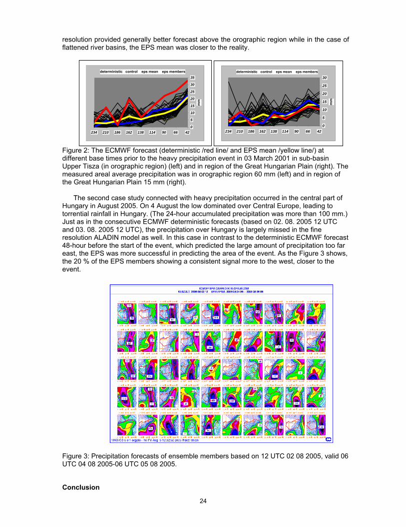
Figure 1: The observed precipitation field in 03. 03. 2001.(left) the precipitation field predicted by ALADIN model (right). Violet areas on the map indicate the predicted precipitation between 50 and 100 mm. The Figure 2 shows the ECMWF forecast (deterministic and EPS mean) at different base times prior to the heavy precipitation event in sub-basin Upper Tisza (in orographic region) and in region of the Great Hungarian Plain in 03 March 2001. The measured areal average precipitation was in orographic region 60 mm and in region of the Great Hungarian Plain 15 mm. The ECMWF model like the ALADIN model underpredicted the precipitation in orgraphic region. At the same time, according to the Figure 2 the deterministic model, due to its higher

24

resolution provided generally better forecast above the orographic region while in the case of flattened river basins, the EPS mean was closer to the reality.

Figure 2: The ECMWF forecast (deterministic /red line/ and EPS mean /yellow line/) at different base times prior to the heavy precipitation event in 03 March 2001 in sub-basin Upper Tisza (in orographic region) (left) and in region of the Great Hungarian Plain (right). The measured areal average precipitation was in orographic region 60 mm (left) and in region of the Great Hungarian Plain 15 mm (right).

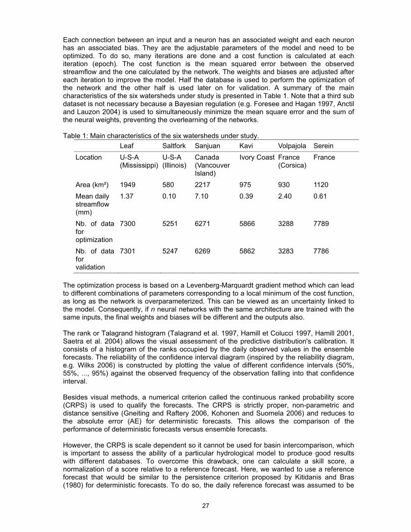
The second case study connected with heavy precipitation occurred in the central part of Hungary in August 2005. On 4 August the low dominated over Central Europe, leading to torrential rainfall in Hungary. (The 24-hour accumulated precipitation was more than 100 mm.) Just as in the consecutive ECMWF deterministic forecasts (based on 02. 08. 2005 12 UTC and 03. 08. 2005 12 UTC), the precipitation over Hungary is largely missed in the fine resolution ALADIN model as well. In this case in contrast to the deterministic ECMWF forecast 48-hour before the start of the event, which predicted the large amount of precipitation too far east, the EPS was more successful in predicting the area of the event. As the Figure 3 shows, the 20 % of the EPS members showing a consistent signal more to the west, closer to the event.

Figure 3: Precipitation forecasts of ensemble members based on 12 UTC 02 08 2005, valid 06 UTC 04 08 2005-06 UTC 05 08 2005.

Conclusion

deterministic control eps mean eps members

0

5

10

15

20

25

30

35

426690114138162186210234

mm

deterministic control eps mean eps members

0

5

10

15

20

25

30

426690114138162186210234

mm

25

According to our verifications the deterministic model has higher skill till day three to four due its higher resolution, while the ensemble mean produces better results after day four to five. However, the first case study shows, in those catchment areas, which are situated in orographic region during heavy precipitation the deterministic version might gives better results after day four to five as well, because this version is more able to capture the effect of orography. At the same time, as the second case study shows, in some convective situations the EPS needs to be taken into account for short range as well.

References I. Bonta, G. Bálint 2003:Meteorological forecasts serving hydrological purposes in Hungary. Poster, International Conference on Advances in Flood Forecasting in Europe Bonta 2006: Performance of the ECMWF model in some interesting synoptic situations , Presentation, Forecast Products Users Meeting, Reading, England ecmwf.int/newsevents/meetings/forecast Users Meeting, Reading, England ecmwf.int/ne

26

Quality assessment of neural networks based hydrological ensemble forecasts by M.A. Boucher¹*, F. Anctil² and L. Perreault³ Quality assessment of neural networks based hydrological ensemble forecasts Marie-Amélie Boucher¹*, François Anctil² and Luc Perreault³ ¹ ² Université Laval, Department of Civil Engineering, Quebec, Canada. ³ Hydro-Quebec, IREQ, Varennes, Canada *Corresponding author: Marie-Amélie Boucher, Université Laval, Department of Civil Engineering, Québec, Qc, G1K 7P4, Canada, 418-656-2131 ext. 8727, marie-a.boucher.1@ulaval.ca Abstract Hydrological ensemble forecasts were constructed with neural networks, a very useful tool regarding its simplicity and execution speed. Here we evaluate the calibration of neural networks based hydrological ensemble forecasts, showing that they exhibit underdispersion. The impact of the bootstrap technique on the calibration has been investigated and led to an improvement of the ensembles’ calibration. The ensemble forecasts were also compared to their deterministic counterpart using the mean continuous ranked probability score and the mean absolute error. The results indicate that the ensemble forecasts perform better than the deterministic ones.

1. Introduction The main objective of this study is to validate daily streamflow predictive distributions obtained with neural networks using the bootstrap technique (Efron and Tibshirani 1993, Breiman 2000). Neural networks have been successfully used in hydrological (e.g. Anctil et al.2004, Hsu et al 1995, Turcotte et al. 2005, Srivastava et al. 2006) and meteorological (Valverde Ramírez et al. 2005, Knutti et al. 2003) modelling. Daily streamflow ensemble forecasts were produced for six watersheds with varied hydrometeorological characteristics. Because of the overparameterization of the neural networks, the training of an ensemble of neural networks leads to an ensemble of solutions. According to Breiman (2000), bootstrapping the inputs to produce an ensemble of forecasts reduces the variance error when taking the ensemble's mean as a deterministic forecast. Here the impact of the bootstrap on the ensembles variability will be evaluated by comparing the performance of ensemble forecasts produced with and without the bootstrap. The ensemble forecasts will be examined with different graphical and numerical methods developed in the meteorological community (e.g. Wilks 2006) and in statistical decision theory (e.g. Good 1952). Their use in the quality assessment of hydrological probabilistic forecasts is more recent (e.g. Weber et al. 2006, Perreault and Gaudet 2004). 2. Methodology Neural networks are nonlinear multivariate regression tools. Although they do not permit explicit modeling of a catchments’ behavior, they perform well in a context of hydrological forecasting and are implemented rapidly. The neural networks used in this study are multilayer perceptrons (MLP) (Rosenblatt 1958). They are commonly encountered in hydrology because they are particularly well adapted for vectorial information. In the actual case, a neural network consists of three layers: the entry layer, the hidden layer (e.g. Lippmann 1987) and the output layer. The entry layer consists in vectors containing the input variables. The inputs are Qt, the streamflow at timestep t, Pt, the precipitation at timestep t, Pt-1, the precipitation at timestep t-1 and Pt-2, the precipitation at time t-2. The hidden layer comprises five neurons with a sigmoid tangent activation function. Finally, the output layer consists of one neuron with a linear activation function, which output is Qt+1, the streamflow at timestep t+1. This architecture follows the results obtained by a previous study by Anctil and Lauzon (2004).

27

Each connection between an input and a neuron has an associated weight and each neuron has an associated bias. They are the adjustable parameters of the model and need to be optimized. To do so, many iterations are done and a cost function is calculated at each iteration (epoch). The cost function is the mean squared error between the observed streamflow and the one calculated by the network. The weights and biases are adjusted after each iteration to improve the model. Half the database is used to perform the optimization of the network and the other half is used later on for validation. A summary of the main characteristics of the six watersheds under study is presented in Table 1. Note that a third sub dataset is not necessary because a Bayesian regulation (e.g. Foresee and Hagan 1997, Anctil and Lauzon 2004) is used to simultaneously minimize the mean square error and the sum of the neural weights, preventing the overlearning of the networks. Table 1: Main characteristics of the six watersheds under study.

Leaf Saltfork Sanjuan Kavi Volpajola Serein Location U-S-A

(Mississippi) U-S-A (Illinois)

Canada (Vancouver Island)

Ivory Coast France (Corsica)

France

Area (km²) 1949 580 2217 975 930 1120 Mean daily streamflow (mm)

1.37 0.10 7.10 0.39 2.40 0.61

Nb. of data for optimization

7300 5251 6271 5866 3288 7789

Nb. of data for validation

7301 5247 6269 5862 3283 7786

The optimization process is based on a Levenberg-Marquardt gradient method which can lead to different combinations of parameters corresponding to a local minimum of the cost function, as long as the network is overparameterized. This can be viewed as an uncertainty linked to the model. Consequently, if n neural networks with the same architecture are trained with the same inputs, the final weights and biases will be different and the outputs also. The rank or Talagrand histogram (Talagrand et al. 1997, Hamill et Colucci 1997, Hamill 2001, Saetra et al. 2004) allows the visual assessment of the predictive distribution's calibration. It consists of a histogram of the ranks occupied by the daily observed values in the ensemble forecasts. The reliability of the confidence interval diagram (inspired by the reliability diagram, e.g. Wilks 2006) is constructed by plotting the value of different confidence intervals (50%, 55%, ..., 95%) against the observed frequency of the observation falling into that confidence interval. Besides visual methods, a numerical criterion called the continuous ranked probability score (CRPS) is used to qualify the forecasts. The CRPS is strictly proper, non-parametric and distance sensitive (Gneiting and Raftery 2006, Kohonen and Suomela 2006) and reduces to the absolute error (AE) for deterministic forecasts. This allows the comparison of the performance of deterministic forecasts versus ensemble forecasts. However, the CRPS is scale dependent so it cannot be used for basin intercomparison, which is important to assess the ability of a particular hydrological model to produce good results with different databases. To overcome this drawback, one can calculate a skill score, a normalization of a score relative to a reference forecast. Here, we wanted to use a reference forecast that would be similar to the persistence criterion proposed by Kitidanis and Bras (1980) for deterministic forecasts. To do so, the daily reference forecast was assumed to be

28

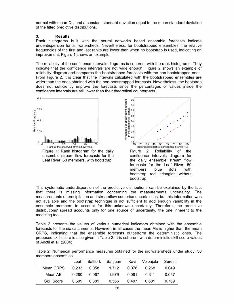
normal with mean Qt-1 and a constant standard deviation equal to the mean standard deviation of the fitted predictive distributions. 3. Results Rank histograms built with the neural networks based ensemble forecasts indicate underdispersion for all watersheds. Nevertheless, for bootstrapped ensembles, the relative frequencies of the first and last ranks are lower than when no bootstrap is used, indicating an improvement. Figure 1 shows an example. The reliability of the confidence intervals diagrams is coherent with the rank histograms. They indicate that the confidence intervals are not wide enough. Figure 2 shows an example of reliability diagram and compares the bootstrapped forecasts with the non-bootstrapped ones. From Figure 2, it is clear that the intervals calculated with the bootstrapped ensembles are wider than the ones obtained with the non-bootstrapped forecasts. Nevertheless, the bootstrap does not sufficiently improve the forecasts since the percentages of values inside the confidence intervals are still lower than their theoretical counterparts.

0 10 20 30 40 500

0.05

0.1

0.15

0.2

Rank of the observed stream flow value

Rel

ativ

e Fr

eque

ncy

15 25 35 45 55 65 75 85 95

15

25

35

45

55

65

75

85

95

Per

cent

age

of o

bser

vatio

ns lo

cate

d in

the

conf

iden

ce in

terv

al

Theoretical length of confidence interval (%) Figure 1: Rank histogram for the daily ensemble stream flow forecasts for the Leaf River, 50 members, with bootstrap.

Figure 2: Reliability of the confidence intervals diagram for the daily ensemble stream flow forecasts for the Leaf River, 50 members, blue dots: with bootstrap, red triangles: without bootstrap.

This systematic underdispersion of the predictive distributions can be explained by the fact that there is missing information concerning the measurements uncertainty. The measurements of precipitation and streamflow comprise uncertainties, but this information was not available and the bootstrap technique is not sufficient to add enough variability in the ensemble members to account for this unknown uncertainty. Therefore, the predictive distributions' spread accounts only for one source of uncertainty, the one inherent to the modeling tool. Table 2 presents the values of various numerical indicators obtained with the ensemble forecasts for the six catchments. However, in all cases the mean AE is higher than the mean CRPS, indicating that the ensemble forecasts outperform the deterministic ones. The proposed skill score is also given in Table 2. It is coherent with deterministic skill score values of Anctil et al. (2004) Table 2: Numerical performance measures obtained for the six watersheds under study, 50 members ensembles.

Leaf Saltfork Sanjuan Kavi Volpajola Serein Mean CRPS 0.233 0.058 1.712 0.078 0.268 0.049

Mean AE 0.280 0.067 1.979 0.081 0.311 0.057 Skill Score 0.699 0.381 0.566 0.497 0.681 0.769

29

References

- Anctil, F. and Lauzon, N. 2004. Generalisation for neural networks through data sampling and training procedures, with applications to streamflow predictions, Hydrology and Earth System Sciences, 8(5), pp.940-958.

- Anctil, F., Perrin, C. and Andréassian, V. 2004. Impact of the length of observed records on the performance of ANN and of conceptual parsimonious rainfall-runoff forecasting models, Environmental Modelling and Software, 19, pp.357-368.

- Breiman, L. 2000. Randomizing Outputs to Increase Prediction Accuracy, MachineLearning, 40, pp.229-242.

- Efron, B. and Tibshirani, R. 1993. An Introduction to the Bootstrap, Chapman and Hall, Londres, 456 pages

- Foresee, F.D. and Hagan, M.T. 1997. Gauss-Newton approximation to Bayesian learning. Proceeding, 1997 IEEE International Conference on Neural Networks, Houston, TX, 3, pp.1930-1935

- Gneiting, T. and A. Raftery. 2006. Strictly Proper Scoring Rules, Prediction, and Estimation, Journal of the American Statistical Association, 102 (477), pp.359-378.

- Good, I.J. 1952. Rational decisions, Journal of the Royal Statistical Society, Serie B, 14, pp.107-114. - Hamill T.N. and Colucci, S.J. 1997. Verification of Eta-RSM Short-Range Ensemble Forecasts, Monthly

Weather Review, 125, pp.1312-1327. - Hamill, T.M. 2001. Interpretation of Rank Histograms for verifying Ensemble Forecasts, Monthly

Weather Review, 129, pp.550-560. - Hsu, K.L., Gupta, H.V. and Sorooshian, S. 1995. Artificial Neural-Network Modeling of the rainfall-runoff

process, Water Resources Research, 31(10), pp.2517-2530. - Kitidanis, P.K. and Bras, R.L. 1980. Real time forecasting with a conceptual hydrologic model: 2.

applications and results, Water Resources Research, 16, pp.1034-1044. - Knutti R., Stocker T.F., Joos F. and Plattner G.-K. 2003. Probabilistic climate change projections using

neural networks., Climate Dynamics, 21, pp.257-272. - Kohonen, J. and Suomela J. 2006. Lessons learned in the challenge: making predictions and scoring

them, Machine Learning Challenges: evaluating predictive uncertainty, visual object classification, and recognizing textual entailment, eds, J. Quiñonero-Candela, et al., Berlin, Springer-Verlag, pp.95-116

- Lippmann, R.P. 1987. An introduction to computing with neural nets. IEEE Acoustics, Speech and signal Processing magazine, 4, pp.4-22.

- Matheson, J.E. and R. L. Winkler 1976. Scoring rules for continuous probability distributions. Management Science, 22, pp.1087-1096.

- Perreault, L. and Gaudet, J., 2004. Contrôle de qualité du système de prévision des apports en eau, Rapport d’étape – Livrable 3.2.5(a), Développement d’un nouvel indicateur hydrologique, IREQ-2004-047c, march 2004, 58 pages.

- Rosenblatt, F. 1958. The Perceptron: a probabilistic model for information storage and organization in the brain, Psychological Review, 65, pp.386-408.

- Saetra, O., Hersbach, H., Bidlot, J.-R. and Richardson, D.S. 2004. Effects of Observations Errors on the Statistics for Ensembles Spread and Reliability, Monthly Weather Review, 132, pp.1487-1501.

- Srivastava, M., Ma, L.Q. and Santos, J.A.G. 2006. Comparison of process-based and artificial neural network approaches for streamflow modeling in an agricultural watershed, Journal of the American Water Resources Association, 42(3), pp.545-563.

- Talagrand, O., R. Vautard. and B. Strauss. 1997. Evaluation of probabilistic prediction systems. Proceedings, ECMWF Workshop on Predictability, Shinfield Park, Reading, Berkshire, ECMWF, pp.1-25.

- Turcotte, R., Favre, A.C., Lacombe, P., Poirier, C. and Villeneuve, J.P. 2005. Estimation des débits sous glace dans le sud du Québec : comparaison de modèles neuronaux et déterministes, Revue Canadienne de Génie Civil, 32, 1pp.1039-1050.

- Valverde Ramírez, M.C., de Campo Velho, H.F. and Ferreira, N.J. 2005. Artificial neural network technique for rainfall forecasting applied to the Sao Paulo region, Journal of Hydrology, 301, pp.146-162.

- Weber, F., Perreault, L. and Fortin, V. 2006. Measuring the performance of hydrological forecasts for hydropower production at BC Hydro and Hydro-Québec, American Meteorological Society, 18th conference on Climate Variability and Change, jan 29th-feb 2nd 2006, Atlanta, Georgia.

- Wilks, D.S. 2006. Statistical Methods in the Atmospheric Sciences, Academic Press, 467 pages.

30

The new ECMWF Variable Resolution Ensemble Prediction System by R. Buizza

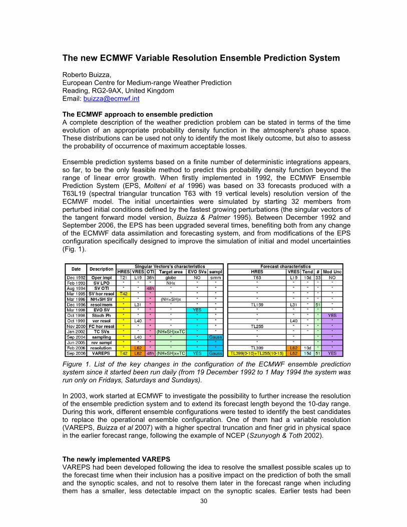
The new ECMWF Variable Resolution Ensemble Prediction System Roberto Buizza, European Centre for Medium-range Weather Prediction Reading, RG2-9AX, United Kingdom Email: buizza@ecmwf.int The ECMWF approach to ensemble prediction A complete description of the weather prediction problem can be stated in terms of the time evolution of an appropriate probability density function in the atmosphere's phase space. These distributions can be used not only to identify the most likely outcome, but also to assess the probability of occurrence of maximum acceptable losses. Ensemble prediction systems based on a finite number of deterministic integrations appears, so far, to be the only feasible method to predict this probability density function beyond the range of linear error growth. When firstly implemented in 1992, the ECMWF Ensemble Prediction System (EPS, Molteni et al 1996) was based on 33 forecasts produced with a T63L19 (spectral triangular truncation T63 with 19 vertical levels) resolution version of the ECMWF model. The initial uncertainties were simulated by starting 32 members from perturbed initial conditions defined by the fastest growing perturbations (the singular vectors of the tangent forward model version, Buizza & Palmer 1995). Between December 1992 and September 2006, the EPS has been upgraded several times, benefiting both from any change of the ECMWF data assimilation and forecasting system, and from modifications of the EPS configuration specifically designed to improve the simulation of initial and model uncertainties (Fig. 1).

Figure 1. List of the key changes in the configuration of the ECMWF ensemble prediction system since it started been run daily (from 19 December 1992 to 1 May 1994 the system was run only on Fridays, Saturdays and Sundays). In 2003, work started at ECMWF to investigate the possibility to further increase the resolution of the ensemble prediction system and to extend its forecast length beyond the 10-day range. During this work, different ensemble configurations were tested to identify the best candidates to replace the operational ensemble configuration. One of them had a variable resolution (VAREPS, Buizza et al 2007) with a higher spectral truncation and finer grid in physical space in the earlier forecast range, following the example of NCEP (Szunyogh & Toth 2002). The newly implemented VAREPS VAREPS had been developed following the idea to resolve the smallest possible scales up to the forecast time when their inclusion has a positive impact on the prediction of both the small and the synoptic scales, and not to resolve them later in the forecast range when including them has a smaller, less detectable impact on the synoptic scales. Earlier tests had been

31

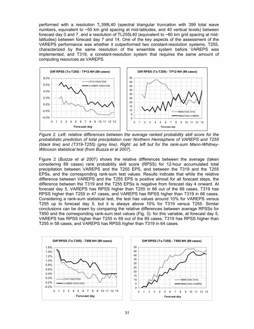
performed with a resolution TL399L40 (spectral triangular truncation with 399 total wave numbers, equivalent to ~50 km grid spacing at mid-latitudes, and 40 vertical levels) between forecast day 0 and 7, and a resolution of TL255L40 (equivalent to ~80 km grid spacing at mid-latitudes) between forecast day 7 and 14. One of the key aspects of the assessment of the VAREPS performance was whether it outperformed two constant-resolution systems, T255, characterized by the same resolution of the ensemble system before VAREPS was implemented, and T319, a constant-resolution system that requires the same amount of computing resources as VAREPS.

Diff RPSS (Tx-T255) - TP12 NH (89 cases)

-4.0%

-2.0%

0.0%

2.0%

4.0%

6.0%

8.0%

0 1 2 3 4 5 6 7 8 9 10 11 12 13

Forecast day

(T319-T255)/T255

(VAREPS-T255)/T255

Diff RPSS (Tx-T255) - TP12 NH (89 cases)

05

101520253035404550

0 1 2 3 4 5 6 7 8 9 10 11 12 13Forecast day

RMW(T255,T319)

RMW(T255,VAREPS)

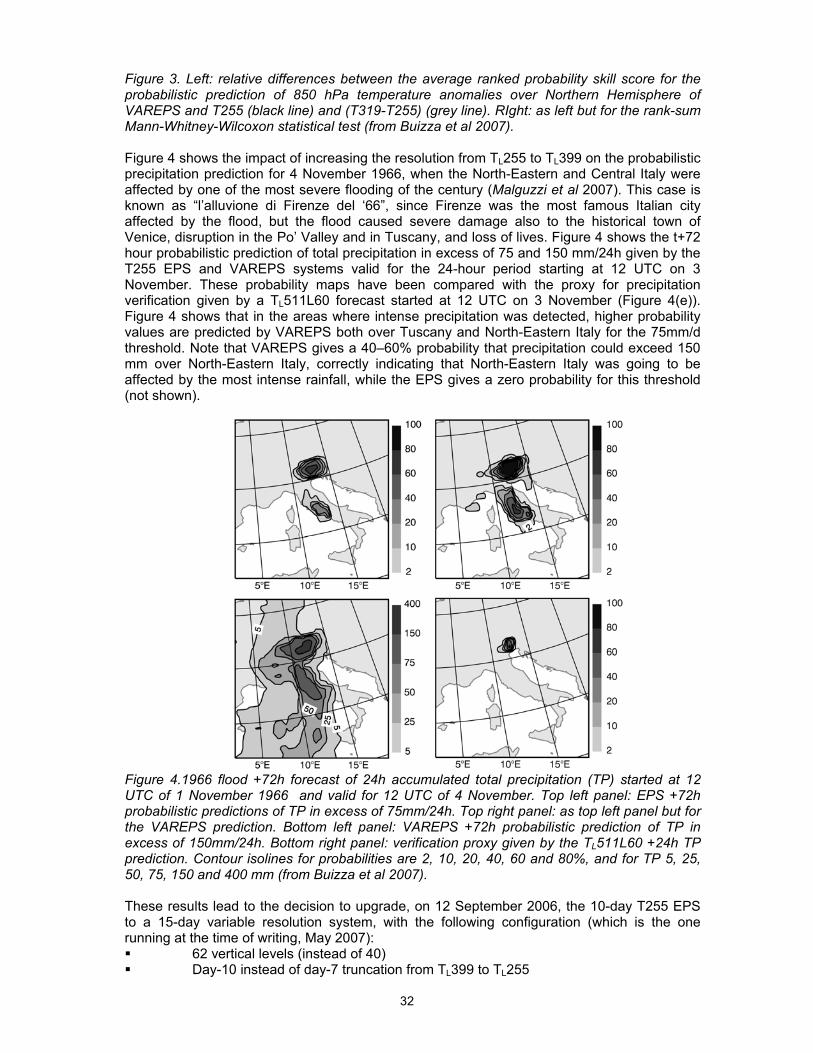
Figure 2. Left: relative differences between the average ranked probability skill score for the probabilistic prediction of total precipitation over Northern Hemisphere of VAREPS and T255 (black line) and (T319-T255) (grey line). Right: as left but for the rank-sum Mann-Whitney-Wilcoxon statistical test (from Buizza et al 2007). Figure 2 (Buizza et al 2007) shows the relative differences between the average (taken considering 89 cases) rank probability skill score (RPSS) for 12-hour accumulated total precipitation between VAREPS and the T255 EPS, and between the T319 and the T255 EPSs, and the corresponding rank-sum test values. Results indicate that while the relative difference between VAREPS and the T255 EPS is positive almost for all forecast steps, the difference between the T319 and the T255 EPSs is negative from forecast day 4 onward. At forecast day 5, VAREPS has RPSS higher than T255 in 66 out of the 89 cases, T319 has RPSS higher than T255 in 47 cases, and VAREPS has RPSS higher than T319 in 66 cases. Considering a rank-sum statistical test, the test has values around 10% for VAREPS versus T255 up to forecast day 5, but it is always above 10% for T319 versus T255. Similar conclusions can be drawn by comparing the relative differences between average RPSSs for T850 and the corresponding rank-sum test values (Fig. 3): for this variable, at forecast day 5, VAREPS has RPSS higher than T255 in 69 out of the 89 cases, T319 has RPSS higher than T255 in 58 cases, and VAREPS has RPSS higher than T319 in 64 cases.

Diff RPSS (Tx-T255) - T850 NH (89 cases)

-0.2%0.0%0.2%0.4%0.6%0.8%1.0%1.2%1.4%1.6%

0 1 2 3 4 5 6 7 8 9 10 11 12 13

Forecast day

(T319-T255)/T255

(VAREPS-T255)/T255

Diff RPSS (Tx-T255) - T850 NH (89 cases)

05

101520253035404550

0 1 2 3 4 5 6 7 8 9 10 11 12 13

Forecast day

RMW(T255,T319)

RMW(T255,VAREPS)

32

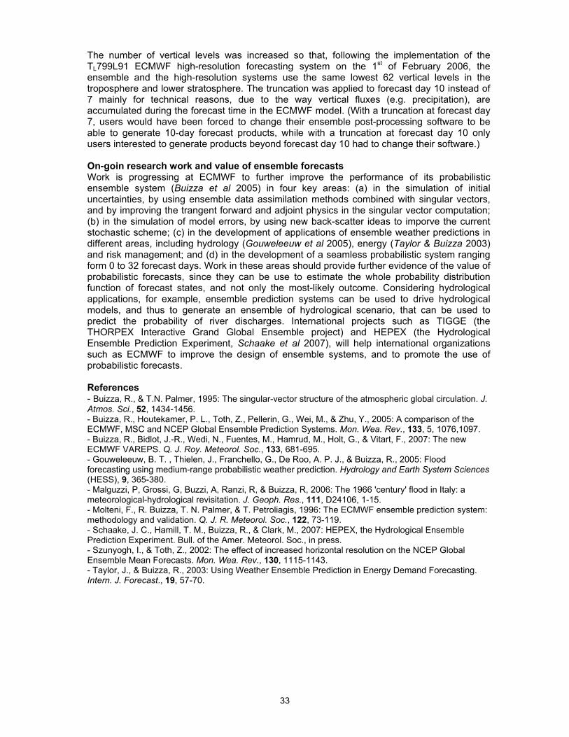
Figure 3. Left: relative differences between the average ranked probability skill score for the probabilistic prediction of 850 hPa temperature anomalies over Northern Hemisphere of VAREPS and T255 (black line) and (T319-T255) (grey line). RIght: as left but for the rank-sum Mann-Whitney-Wilcoxon statistical test (from Buizza et al 2007). Figure 4 shows the impact of increasing the resolution from TL255 to TL399 on the probabilistic precipitation prediction for 4 November 1966, when the North-Eastern and Central Italy were affected by one of the most severe flooding of the century (Malguzzi et al 2007). This case is known as “l’alluvione di Firenze del ‘66”, since Firenze was the most famous Italian city affected by the flood, but the flood caused severe damage also to the historical town of Venice, disruption in the Po’ Valley and in Tuscany, and loss of lives. Figure 4 shows the t+72 hour probabilistic prediction of total precipitation in excess of 75 and 150 mm/24h given by the T255 EPS and VAREPS systems valid for the 24-hour period starting at 12 UTC on 3 November. These probability maps have been compared with the proxy for precipitation verification given by a TL511L60 forecast started at 12 UTC on 3 November (Figure 4(e)). Figure 4 shows that in the areas where intense precipitation was detected, higher probability values are predicted by VAREPS both over Tuscany and North-Eastern Italy for the 75mm/d threshold. Note that VAREPS gives a 40–60% probability that precipitation could exceed 150 mm over North-Eastern Italy, correctly indicating that North-Eastern Italy was going to be affected by the most intense rainfall, while the EPS gives a zero probability for this threshold (not shown).

Figure 4.1966 flood +72h forecast of 24h accumulated total precipitation (TP) started at 12 UTC of 1 November 1966 and valid for 12 UTC of 4 November. Top left panel: EPS +72h probabilistic predictions of TP in excess of 75mm/24h. Top right panel: as top left panel but for the VAREPS prediction. Bottom left panel: VAREPS +72h probabilistic prediction of TP in excess of 150mm/24h. Bottom right panel: verification proxy given by the TL511L60 +24h TP prediction. Contour isolines for probabilities are 2, 10, 20, 40, 60 and 80%, and for TP 5, 25, 50, 75, 150 and 400 mm (from Buizza et al 2007). These results lead to the decision to upgrade, on 12 September 2006, the 10-day T255 EPS to a 15-day variable resolution system, with the following configuration (which is the one running at the time of writing, May 2007): 62 vertical levels (instead of 40) Day-10 instead of day-7 truncation from TL399 to TL255

33

The number of vertical levels was increased so that, following the implementation of the TL799L91 ECMWF high-resolution forecasting system on the 1st of February 2006, the ensemble and the high-resolution systems use the same lowest 62 vertical levels in the troposphere and lower stratosphere. The truncation was applied to forecast day 10 instead of 7 mainly for technical reasons, due to the way vertical fluxes (e.g. precipitation), are accumulated during the forecast time in the ECMWF model. (With a truncation at forecast day 7, users would have been forced to change their ensemble post-processing software to be able to generate 10-day forecast products, while with a truncation at forecast day 10 only users interested to generate products beyond forecast day 10 had to change their software.) On-goin research work and value of ensemble forecasts Work is progressing at ECMWF to further improve the performance of its probabilistic ensemble system (Buizza et al 2005) in four key areas: (a) in the simulation of initial uncertainties, by using ensemble data assimilation methods combined with singular vectors, and by improving the trangent forward and adjoint physics in the singular vector computation; (b) in the simulation of model errors, by using new back-scatter ideas to imporve the current stochastic scheme; (c) in the development of applications of ensemble weather predictions in different areas, including hydrology (Gouweleeuw et al 2005), energy (Taylor & Buizza 2003) and risk management; and (d) in the development of a seamless probabilistic system ranging form 0 to 32 forecast days. Work in these areas should provide further evidence of the value of probabilistic forecasts, since they can be use to estimate the whole probability distribution function of forecast states, and not only the most-likely outcome. Considering hydrological applications, for example, ensemble prediction systems can be used to drive hydrological models, and thus to generate an ensemble of hydrological scenario, that can be used to predict the probability of river discharges. International projects such as TIGGE (the THORPEX Interactive Grand Global Ensemble project) and HEPEX (the Hydrological Ensemble Prediction Experiment, Schaake et al 2007), will help international organizations such as ECMWF to improve the design of ensemble systems, and to promote the use of probabilistic forecasts. References - Buizza, R., & T.N. Palmer, 1995: The singular-vector structure of the atmospheric global circulation. J. Atmos. Sci., 52, 1434-1456. - Buizza, R., Houtekamer, P. L., Toth, Z., Pellerin, G., Wei, M., & Zhu, Y., 2005: A comparison of the ECMWF, MSC and NCEP Global Ensemble Prediction Systems. Mon. Wea. Rev., 133, 5, 1076,1097. - Buizza, R., Bidlot, J.-R., Wedi, N., Fuentes, M., Hamrud, M., Holt, G., & Vitart, F., 2007: The new ECMWF VAREPS. Q. J. Roy. Meteorol. Soc., 133, 681-695. - Gouweleeuw, B. T. , Thielen, J., Franchello, G., De Roo, A. P. J., & Buizza, R., 2005: Flood forecasting using medium-range probabilistic weather prediction. Hydrology and Earth System Sciences (HESS), 9, 365-380. - Malguzzi, P, Grossi, G, Buzzi, A, Ranzi, R, & Buizza, R, 2006: The 1966 'century' flood in Italy: a meteorological-hydrological revisitation. J. Geoph. Res., 111, D24106, 1-15. - Molteni, F., R. Buizza, T. N. Palmer, & T. Petroliagis, 1996: The ECMWF ensemble prediction system: methodology and validation. Q. J. R. Meteorol. Soc., 122, 73-119. - Schaake, J. C., Hamill, T. M., Buizza, R., & Clark, M., 2007: HEPEX, the Hydrological Ensemble Prediction Experiment. Bull. of the Amer. Meteorol. Soc., in press. - Szunyogh, I., & Toth, Z., 2002: The effect of increased horizontal resolution on the NCEP Global Ensemble Mean Forecasts. Mon. Wea. Rev., 130, 1115-1143. - Taylor, J., & Buizza, R., 2003: Using Weather Ensemble Prediction in Energy Demand Forecasting. Intern. J. Forecast., 19, 57-70.

34

C-D

Application of meteorological ensemles for Danube flood forecasting and warning by A. Csík, G. Bálint*, P.Bartha and B. Gauzer APPLICATION OF METEOROLOGICAL ENSEMBLES FOR DANUBE FLOOD FORECASTING AND WARNING András Csík, Gábor Bálint*, Péter Bartha and Balázs Gauzer VITUKI Enviromental Protection and Water Management Research Institute, Kvassay 1, Budapest, Hungary *Corresponding author: Gábor Bálint, tel.: 003612155001, e-mail: balint@vituki.hu Abstract Flood forecasting schemes may have the most diverse structure depending on catchment size, response or concentration time and the availability of real time input data. The centre of weight of the hydrological forecasting system is often shifted from hydrological tools to the meteorological observation and forecasting systems. At lowland river sections simple flood routing techniques prevail where accuracy of discharge estimation might depend mostly on the accuracy of upstream discharge estimation. In large river basin systems both elements are present. Attempts are made enabling the use of ensemble of short and medium term meteorological forecast results for real-time flood forecasting by coupling meteorological and hydrological modelling tools. 1. Components of the flood forecasting system Flood forecasting provides essential information for flood defence. This type of information is handled within the national Flood Management Information System in Hungary. Transit flow originating from the upstream parts of the upper and central Danube Basin dominates hydrological regime of Hungarian rivers consequently hydrological systems cover an area of more than 300,000 km2 mostly outside of the national boundary. The central unit of the forecasting system is operated for the 210,000 km2 catchment of River Danube upstream of the southern border, limited by the cross section near the town of Mohács. Separate units deal with tributaries Tisza and Dráva. All three units are managed by the National Hydrological Forecasting Service (NHFS) within the Water Resources Research Centre. The present paper concerns only Danube proper, which is the recipient of German, Austrian and Slovak tributaries. The Danube forecasting system is linked to the METINFO system of the Hungarian Meteorological Service providing meteorological forecasts and observations. The hydrological data collection and pre-processing system linked to similar services of the Danube countries handles part of the meteorological data and water level and discharge data of more than 90 hydrological observation sites. The NHFS modeling system performs data assimilation and produces 12-hour water level and discharge forecast 6 days ahead for 46 forecast stations. 1.1. METINFO - meteorological forecasts and other products The European Centre for Medium-Range Weather Forecasts (ECMWF) products are used up to 10 days ahead. Another input is forecasts by LACE (Limited Area Modeling for Central Europe) model which covers the upper and central part of the Danube basin. Some of the Members run the local version of the ALADIN model centered for their territory providing an even more precise and exact short-range forecasts for the forecasters. 1.2. The hydrological modeling system The NHFS GAPI/TAPI modeling system has been developed within the Hydrological Institute of the VITUKI Centre. The conceptual, partly physically-based GAPI model serves for simulations and forecasting of flow for medium and large drainage basins. The lumped system consists of sub-basins and flood routing sections. In the course of a decade of development and upgrading the forecasting package has grown

35

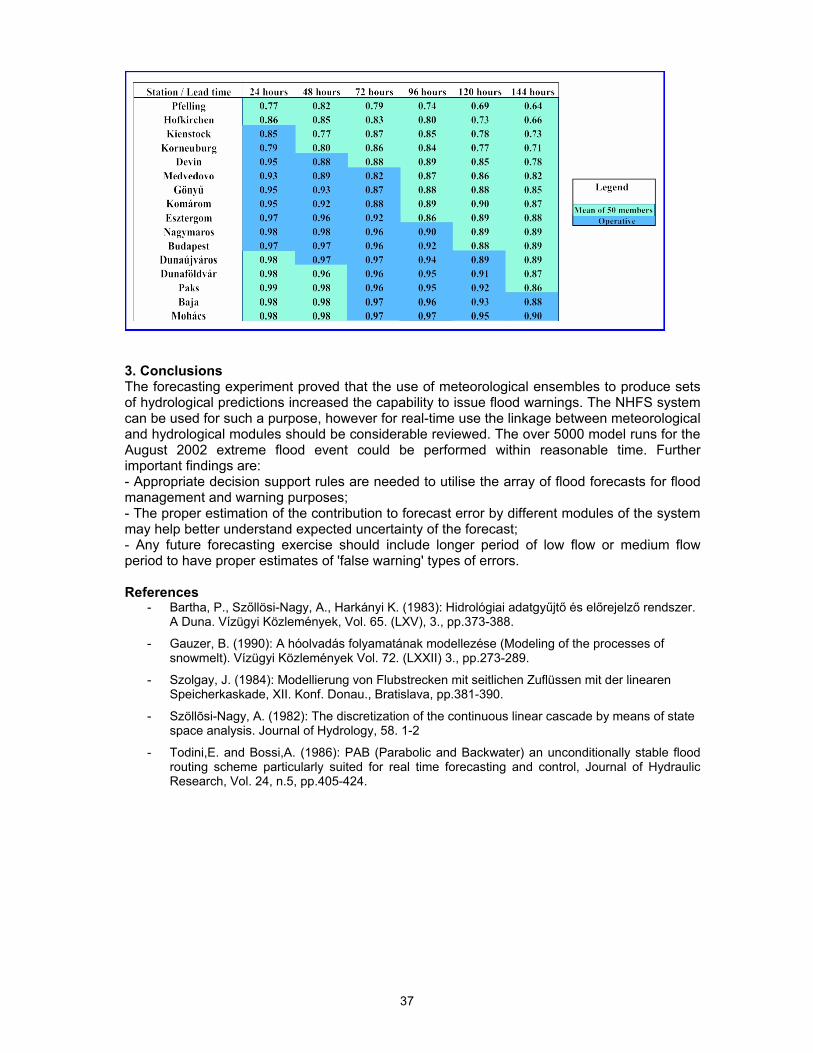
into a complex tool containing snow accumulation and snowmelt, soil frost, effective rainfall, runoff and flood routing modules, extended with statistical error correction - continuous updating and hydraulic - 'empirical backwater effect' modules. The Discrete Linear Cascade Model (DLCM) developed by Szőllösi-Nagy (1982) utilizing an approach similar to the one reported by Szolgay (1984) serves for the routing of flow components and channel routing. First version of the complex GAPI model with modular structure was designed by Bartha et al. (1983). The choice of the model was proved by a number of inter-comparison studies. The first model version was extended by a snowmelt module (Gauzer, 1990) and the complexity of the system was raised gradually. The backwater module utilizes simplifications similar those suggested by Todini and Bossi (1986). The large number of nodes (69) makes the system in fact semi distributed in basin scale. Out of the total number of nodes 46 are related to forecast stations. Real time mode runs are carried out in 12 hourly time steps. Input/output values and state variables of the precipitation - runoff modules are integrated over sub-basins as weighted or simple arithmetic average of station or grid values. A special procedure was designed to interpolate sparse grid data of ECMWF products. The rapid growth of resolution and forecast range of numerical weather prediction models enabled the use of their result for hydrological forecasting purposes. 2. The use of meteorological ensembles for flood forecasting 2.1. Testing on an extreme event Operational use of the above system often revealed the uncertainty of QPF taken into consideration while calculating expected Danube hydrographs. To test the feasibility of the use of meteorological ensembles a forecasting experiment was designed. The aim of the investigation was also to assess how much prior estimates of uncertainty of can be given by the selected approach. ECMWF archived forecast arrays were retrieved. Partly the standard data ingestion part of the NHFS system was used. 52 sets of input data arrays were produced using the 50 ECMWF ensemble elements, additionally deterministic and control runs were also carried. Control run input is identically produced as the deterministic one, but instead if the 40 km resolution 80 km resolution is used. The period of July-August 2002 was selected including the period of the August flood. The calculation of the ensemble forecast is time demanding that is why the standard operational procedure was modified, flags and options were reduced to produce batch type of processing. (All together more than 5000 runs were performed which equals more than 6 years 'real time' activity.) 12 hour time step 1-6 day ahead forecast were calculated for 46 forecast stations. Out of those 21 were analysed comparing forecast results to observed hydrographs. 2.2. Results Figure 1 shows main features of different sets of hydrological ensembles for gauging stations Devin and Budapest. The specific Box-Whisker diagrams indicate beside observed hydrographs forecast arrays showing minimum and maximum values of 50 element ensembles while quartiles above and below the mean values are indicated by wider boxes. Forecast is indicated for 24, 72, 144 hours of lead time. Even this two gauge comparison is sufficient to indicate the impact of growing travel time along the 200 km reach which is expressed in higher accuracy of forecast at the lower (Budapest) section while the rainfall - runoff module has higher weight at Devin, consequently forecast error is higher at the upstream station. The natural increase of error with the lead time can also be followed. Upstream rainfall induced flood waves have an impact on Budapest section only 2-3 days after the rainfall (or snowmelt) event occurs. The limit of predictability is reached at Devin at the 6th day, however ensemble means still give some useful information. Forecast types are compare with each other on the Table 1. The basic of the comparison was a in hydrology widely used skill score, so-called efficiency coefficient. This table refers to the period 21 July – 31 August 2002 and the colors shows more efficient forecast type. In case of the upper section and higher lead time the mean of 50 members is better because the precipitation forecast is dominant in the hydrological forecast with high (3-6 days) lead time. Down to the stream – when the flow routing is dominant – the operative forecast gives the

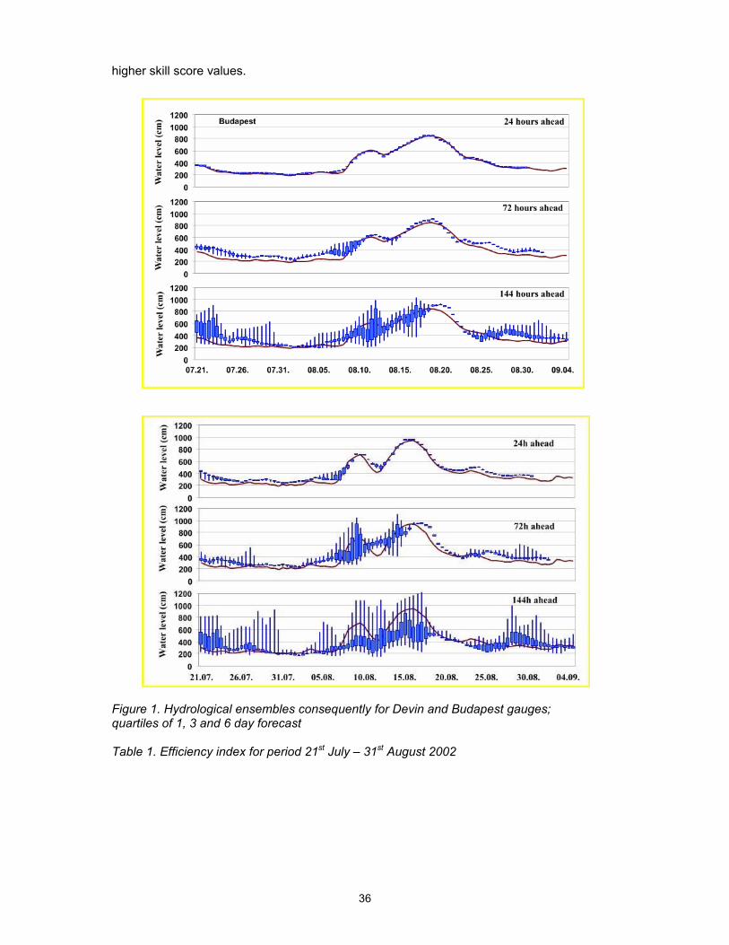
36

higher skill score values.

Figure 1. Hydrological ensembles consequently for Devin and Budapest gauges; quartiles of 1, 3 and 6 day forecast Table 1. Efficiency index for period 21st July – 31st August 2002

37

3. Conclusions The forecasting experiment proved that the use of meteorological ensembles to produce sets of hydrological predictions increased the capability to issue flood warnings. The NHFS system can be used for such a purpose, however for real-time use the linkage between meteorological and hydrological modules should be considerable reviewed. The over 5000 model runs for the August 2002 extreme flood event could be performed within reasonable time. Further important findings are: - Appropriate decision support rules are needed to utilise the array of flood forecasts for flood management and warning purposes; - The proper estimation of the contribution to forecast error by different modules of the system may help better understand expected uncertainty of the forecast; - Any future forecasting exercise should include longer period of low flow or medium flow period to have proper estimates of 'false warning' types of errors. References

- Bartha, P., Szőllösi-Nagy, A., Harkányi K. (1983): Hidrológiai adatgyűjtő és előrejelző rendszer. A Duna. Vízügyi Közlemények, Vol. 65. (LXV), 3., pp.373-388.

- Gauzer, B. (1990): A hóolvadás folyamatának modellezése (Modeling of the processes of snowmelt). Vízügyi Közlemények Vol. 72. (LXXII) 3., pp.273-289.

- Szolgay, J. (1984): Modellierung von Flubstrecken mit seitlichen Zuflüssen mit der linearen Speicherkaskade, XII. Konf. Donau., Bratislava, pp.381-390.

- Szöllõsi-Nagy, A. (1982): The discretization of the continuous linear cascade by means of state space analysis. Journal of Hydrology, 58. 1-2

- Todini,E. and Bossi,A. (1986): PAB (Parabolic and Backwater) an unconditionally stable flood routing scheme particularly suited for real time forecasting and control, Journal of Hydraulic Research, Vol. 24, n.5, pp.405-424.

38

How should we compare hydrological models by R. T. Clarke

How should we compare hydrological models? Robin T Clarke Instituto de Pesquisas Hidráulicas (IPH-UFRGS) Porto Alegre – RS, Brazil. Abstract Whether or not hydrological models of rainfall-runoff processes use precipitation forecasts, there is an ever-growing need to compare the performances of different models. This paper argues that much more attention needs to be paid to aspects of experimental design when making model comparisons. At present, a typical procedure is as follows: (i) models are suggested for inclusion by their proponents; (ii) a set of watersheds with “reliable” hydrological records is selected as a basis for model comparison, with each model to be tested on each watershed; (iii) a part of the record of each watershed is selected for model calibration, with each model calibrated by its proponent, but with no particular specified order for the watersheds used; (iv) another part of the record from each watershed is issued for model verification, with each model verified by its proponent, in no particular specified order; (v) pre-selected measures of model performance, denoted generically by X, are calculated for both calibration and verification procedures; (vi) the values X given by different models are compared and conclusions drawn. As an experimental design, this can be criticized on a number of counts which include, but are not limited to, the following: (i) it is not the models which are being compared, but the models as used by their proponents (running counter to the basic requirement of all science that results should be reproducible by other researchers); (ii) since each model is tested on each watershed’s data by the model’s proponents, factors of user fatigue and/or learning may introduce bias, particularly where model calibration involves elements of subjective decision-making; (iii) the design gives no valid estimate of the uncertainty in the measures X of model performance. Much greater care is needed to address such issues, which arise not only in the comparison of hydrological models, but wherever alternative models of complex environmental phenomena are to be compared. It is argued that much can be learned from the classical discipline of experimental design as widely practiced in other fields of scientific endeavour.

39

Discharge ensemble forecasts based on the COSMO-LEPS quantitative precipitation by T. Diomede, C. Marsigli, A. Montani and T. Paccagnella DISCHARGE ENSEMBLE FORECASTS BASED ON THE COSMO-LEPS QUANTITATIVE PRECIPITATION Tommaso Diomede1,2*, Chiara Marsigli1, Andrea Montani1, Tiziana Paccagnella1 1 Regional Hydro-Meteorological Service ARPA-SIM, Bologna, Italy 2 Centro Interuniversitario di Ricerca in Monitoraggio Ambientale (CIMA), Università degli studi di Genova e della Basilicata, Savona, Italy * Corresponding author: Tommaso Diomede, Viale Silvani 6 40122 Bologna Italy, +390516497512, tdiomede@arpa.emr.it Abstract In the present study the usefulness and the skill of the meteorological mesoscale ensemble prediction system COSMO-LEPS is evaluated as a tool to operationally supply quantitative precipitation forecasts driving a meteo-hydrological coupled system aimed at providing reliable real-time discharge ensemble forecasts for the Reno river basin, a medium-size catchment in northern Italy. The hydrological simulations are carried out by means of the distributed rainfall-runoff model TOPKAPI. The performance of the proposed probabilistic forecasting chain is evaluated simulating the streamflow forecasts provided for the autumn seasons of the period 2003-2005. The deterministic forecasting chain, operationally implemented, based on the same rainfall-runoff model fed with the precipitation forecast provided by the COSMO model-suite LAMI is used as term of comparison. 1. Introduction The quantitative precipitation forecast (QPF) is still a challenging task at the scales of interest for hydrological predictions. Although the use of high resolution limited-area models (LAMs) has improved the short-range prediction of locally intense events, it is sometimes difficult to forecast accurately their space-time evolution, especially for ranges longer than 48 hours

(Marsigli et al., 2005). Nowadays, the ensemble prediction techniques are widely used in the meteorological community, allowing to add probabilistic information to the forecasts, especially with respect to risk-related events. Moreover, meteorological ensemble systems have recently

been used to provide a probabilistic input to hydrological forecasts, in order to improve both the accuracy of these forecasts and the reliability of uncertainty estimates.

In this work, the use of a Limited Ensemble Predictions System (LEPS) is considered as the meteorological contribution to a meteo-hydrological probabilistic forecasting chain. In this way, the estimate of uncertainty affecting hydrological model predictions is related with the problem to integrate meteorological forecast uncertainty into a hydrological model capable to propagate

it into hydrological forecast and warning uncertainty.

2. Methodology The proposed probabilistic flood forecasting chain is based on the following tools: - COSMO-LEPS, a Limited-area Ensemble Prediction System based on the non-hydrostatic limited-area model COSMO, daily running (12 UTC) at ECMWF (European Centre for Medium-Range Weather Forecasts) since November 2002; - TOPKAPI (TOPographic Kinematic APproximation and Integration), a physically-based distributed rainfall-runoff model model (Todini and Ciarapica, 2001). The LEPS methodology, described in its essential principles in Molteni et al. (2001) and Marsigli et al. (2001), is designed to combine the advantages of a global-ensemble prediction system with the ability typical of LAMs to detail atmospheric phenomena on more local scales, particularly in those regions dominated by the effects of complex orography

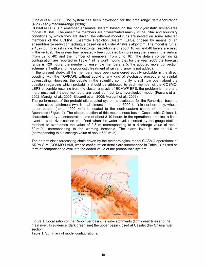
40

(Tibaldi et al., 2006). The system has been developed for the time range “late-short-range (48h) - early-medium-range (120h)”. COSMO-LEPS is 16-member ensemble system based on the non-hydrostatic limited-area model COSMO. The ensemble members are differentiated mainly in the initial and boundary conditions by which they are driven: the different model runs are nested on some selected members of the ECMWF Ensemble Prediction System (EPS), chosen by means of an ensemble-size reduction technique based on a Cluster Analysis algorithm. The model is run at a 132-hour forecast range, the horizontal resolution is of about 10 km and 40 layers are used in the vertical. The system has repeatedly been updated by increasing the layers in the vertical (from 32 to 40) and the number of members (from 5 to 16). The details concerning its configuration are reported in Table 1 (it is worth noting that for the year 2003 the forecast range is 120 hours, the number of ensemble members is 5, the adopted moist convection scheme is Tiedtke and the prognostic treatment of rain and snow is not added). In the present study, all the members have been considered equally probable in the direct coupling with the TOPKAPI, without applying any kind of stochastic procedure for rainfall downscaling. However, the debate in the scientific community is still now open about the question regarding which probability should be attributed to each member of the COSMO-LEPS ensemble resulting from the cluster analysis of ECMWF EPS; the problem is more and more unsolved if these members are used as input to a hydrological model (Ferraris et al., 2002; Marsigli et al., 2005; Siccardi et al., 2005; Verbunt et al., 2006). The performance of the probabilistic coupled system is evaluated for the Reno river basin, a medium-sized catchment (which total dimension is about 5000 km2) in northern Italy, whose upper portion (about 1000 km2) is located to the north-eastern slopes of the northern Apennines (Figure 1). The closure section of this mountainous basin, Casalecchio Chiusa, is characterized by a concentration time of about 8-10 hours. In the operational practice, a flood event at such river section is defined when the water level, recorded by the gauge station, reaches or overcomes the value of 0.8 m (corresponding to a discharge value of about 80 m3/s), corresponding to the warning threshold. The alarm level is set to 1.6 m (corresponding to a discharge value of about 630 m3/s). The deterministic forecasting chain driven by the meteorological model COSMO operational at ARPA-SIM (COSMO-LAMI, whose configuration details are summarised in Table 1) is used as term of comparison to evaluate the added value of the probabilistic system.

Casalecchio Chiusa

Emilia-RomagnaRegion

Figure 1. Localisation of the Reno river basin, its sub-catchments (light green line) and the main river. In evidence (dark green line) the upper basin closed at Casalecchio Chiusa river section. Table 1. Summary of model configurations.

41

Name

COSMO-LEPS

COSMO-LAMI

Boundaryconditions

EPS forecasts

DWD-GMEforecasts

Initialconditions

EPS analyses

LAMI mesoscaleassimilation (nudging)

Moistconvection

Tiedtke or Kain-Fritsch(randomly selected)

implicit(Tiedtke)

Prognosticprecipitation

yes

no

Horizontalresolution

10 km

7 km

Verticalresolution

32 layers

35 layers

Forecastrange

132 h

72 h

Numberof members

10

1

3. Results Discharge predictions based on the COSMO-LEPS ensemble precipitation forecasts have been computed for the autumn seasons of the years 2003, 2004 and 2005. A statistical analysis, in terms of mean error and root mean squared error, is carried out on the ensemble of hourly discharge forecasts to investigate which quantile is more suitable to represent the ensemble forecast and to compare the performance of the probabilistic approach with the corresponding one provided by the deterministic forecasting chain. From the computations (shown in Figures 2 and 3 only for the autumn 2003) it derives that:

- the 80% and 90% quantiles perform generally better with respect to the ensemble mean as the lead-time increases. This trend is more evident when the autumn season is characterised by higher streamflow values (years 2003 and 2004).

- the performance decay of the probabilistic coupled system is evident up to the first 48-hour forecast range; for higher lead-times, the decay is partly compensated by the ensemble skill.

- the discharge simulations based on the deterministic precipitation forecast perform slightly better for the first 24-hour range. The added value of the probabilistic system comes out in the next forecast ranges.

A further analysis (whose results are not shown) has been carried out about the verification of warnings and alarms based on the predicted discharges:

- for the warning level, the false alarms provided by the higher quantiles (80% and 90%) of the probabilistic forecasting chain do not increase considerably with respect to the ones produced by the deterministic chain, except for the 90% quantile in autumn 2005; on the other hand, if the higher quantiles are considered, the miss events decrease with respect to those obtained with the ensemble mean or the deterministic forecast;

- for the alarm level, if the 90% quantile is considered, no false alarms would have been issued by the probabilistic forecasting chain, whereas one false alarm would have been issued by the deterministic one for a case in autumn 2005; about the miss events, both the forecasting chains fail the forecast of the three events occurred (two in autumn 2003, one in autumn 2004).

Generally, we can conclude that the discharge predictions based on the COSMO-LEPS ensemble precipitation forecasts show performance which are comparable to the single-valued forecast driven by COSMO-LAMI for the first 24-hour forecast range. The added value of the probabilistic system comes out with increasing lead-times, especially starting from the +48-72 forecast range. The timing of the streamflow simulations driven by COSMO-LEPS matches quite well the event occurrence and the number of false alarms is limited, also with the lead-time increasing. On the other hand, the prediction of the event magnitude is less accurate, especially for the higher streamflows, usually underestimated.

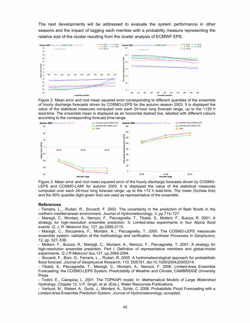
42

The next developments will be addressed to evaluate the system performance in other seasons and the impact of tagging each member with a probability measure representing the relative size of the cluster resulting from the cluster analysis of ECMWF EPS.

Autumn 2003 mean error COSMO-LEPS fc +00-120 h

-30

-25

-20

-15

-10

-5

0

5

10

15

20

25

30

35

q05 q10 q20 q25 q40 q50 q60 q75 q80 q90 q95

ensemble quantiles

mea

n er

ror (

m3 /s

)

fc +00-24 fc +24-48fc +48-72 fc +72-96fc +96-120_ _ _ _ ensemble mean

Autumn 2003 root mean squared error COSMO-LEPS fc +00-120 h

10

30

50

70

90

110

130

q05 q10 q20 q25 q40 q50 q60 q75 q80 q90 q95ensemble quantiles

root

mea

n sq

uare

d er

ror (

m3 /s

)

fc +00-24 fc +24-48fc +48-72 fc +72-96fc +96-120_ _ _ _ ensemble mean

Figure 2. Mean error and root mean squared error corresponding to different quantiles of the ensemble of hourly discharge forecasts driven by COSMO-LEPS for the autumn season 2003. It is displayed the value of the statistical measures computed over each 24-hour long forecast range, up to the +120 h lead-time. The ensemble mean is displayed as an horizontal dashed line, labelled with different colours according to the corresponding forecast time-range. Autumn 2003 mean error fc +00-72 h

-40

-30

-20

-10

0

10

20

30

00-24 24-48 48-72

forecast range

mea

n er

ror (

m3 /s

)

ensemble mean COSMO-LEPSensemble q90 COSMO-LEPSLAMI

Autumn 2003 root mean squared error fc +00-72 h

0

20

40

60

80

100

120

140

160

00-24 24-48 48-72forecast range

root

mea

n sq

uare

d er

ror (

m3 /s

)ensemble mean COSMO-LEPS

ensemble q90 COSMO-LEPSLAMI

Figure 3. Mean error and root mean squared error of the hourly discharge forecasts driven by COSMO-LEPS and COSMO-LAMI for autumn 2003. It is displayed the value of the statistical measures computed over each 24-hour long forecast range, up to the +72 h lead-time. The mean (fuchsia line) and the 90% quantile (light green line) are used as representative of the ensemble. References - Ferraris, L.., Rudari, R., Siccardi, F. 2002. The uncertainty in the prediction of flash floods in the northern mediterranean environment. Journal of Hydrometeorology, 3, pp.714–727. - Marsigli, C., Montani, A., Nerozzi, F., Paccagnella, T., Tibaldi, S., Molteni, F., Buizza, R. 2001. A strategy for high-resolution ensemble prediction. II: Limited-area experiments in four Alpine flood events. Q. J. R. Meteorol Soc, 127, pp.2095-2115. - Marsigli, C., Boccanera, F., Montani, A.., Paccagnella, T. 2005. The COSMO-LEPS mesoscale ensemble system: validation of the methodology and verification. Nonlinear Processes in Geophysics, 12, pp. 527–536. - Molteni, F., Buizza, R., Marsigli, C., Montani, A., Nerozzi, F., Paccagnella, T. 2001. A strategy for high-resolution ensemble prediction. Part I: Definition of representative members and global-model experiments. Q J R Meteorol Soc,127, pp.2069-2094. - Siccardi, F., Boni, G., Ferraris, L.., Rudari, R. 2005. A hydrometeorological approach for probabilistic flood forecast. Journal of Geophysical Research, 110: D05101, doi:10.1029/2004JD005314. - Tibaldi, S., Paccagnella, T., Marsigli, C., Montani, A., Nerozzi, F. 2006. Limited-Area Ensemble Forecasting: the COSMO-LEPS System. Predictabilty of Weather and Climate, CAMBRIDGE University Press - Todini, E., Ciarapica, L. 2001. The TOPKAPI model. In: Mathematical Models of Large Watershed Hydrology, Chapter 12, V.P. Singh. et al. (Eds.), Water Resources Publications. - Verbunt, M., Walser, A., Gurtz, J., Montani, A., Schär, C. 2006. Probabilistic Flood Forecasting with a Limited-Area Ensemble Prediction System. Journal of Hydrometeorology, accepted.

43

A meteo-hydrological prediction system based on a multi-model approach for ensemble precipitation forecasting by T. Diomede, S. Davolio, C. Marsigli, M. M. Miglietta, A. Morgillo and A. Moscatello

A METEO-HYDROLOGICAL PREDICTION SYSTEM BASED ON A MULTI-MODEL APPROACH FOR ENSEMBLE PRECIPITATION FORECASTING Tommaso Diomede1,4*, Silvio Davolio2, Chiara Marsigli1, Mario Marcello Miglietta3, Antonella Morgillo1, Agata Moscatello3

1 Regional Hydro-Meteorological Service ARPA-SIM, Bologna, Italy 2 Institute of Atmospheric Sciences and Climate of the Italian National Research Council (ISAC-CNR), Bologna, Italy 3 Institute of Atmospheric Sciences and Climate of the Italian National Research Council (ISAC-CNR), Lecce, Italy 4 Centro Interuniversitario di Ricerca in Monitoraggio Ambientale (CIMA), Università degli studi di Genova e della Basilicata, Savona, Italy * Corresponding author: Tommaso Diomede, Viale Silvani 6 40122 Bologna Italy, +390516497512, tdiomede@arpa.emr.it Abstract The precipitation predicted by a numerical weather prediction model, even at high resolution, suffers from errors which can be considerable at the scales of interest for hydrological purposes. In the present study, the uncertainty related to the meteorological model error is taken into account by implementing a multi-model forecasting approach, aimed at providing multiple future precipitation scenarios driving the same hydrological model. Therefore, the estimation of the uncertainty associated with the meteorological prediction can be exploited by the hydrological model, propagating the error into the hydrological forecast. The proposed meteo-hydrological forecasting system is implemented in a real-time configuration for several episodes of intense precipitation affecting the Reno river basin, located in northern Italy (Apennines). The episodes are associated with flood events of different intensity. The coupled system seems promising in order to provide useful information concerning the discharge peaks (amount and timing) for warning purposes. 1. Introduction In order to extend the lead time between warning and occurrence of a flood event, an appropriate prediction of the hydrological responses for medium-sized catchments (from 1000 to 10000 km2) is only possible if hydrological models are coupled with numerical weather prediction (NWP) models, using the predictive potential of both the atmospheric and the hydrological models. This approach suffers from several sources of uncertainty, lying in the hydrological and meteorological models themselves; however, for real-time forecasting the error in rainfall prediction prevails on the other sources of uncertainty (Krzysztofowicz, 1999). To cope and deal with the above uncertainties, ensemble forecasting techniques are beginning to be applied to hydrological prediction. The scientific community has recognized the importance of dealing with uncertainty, especially with respect to risk-related events, and has started to use this concept in hydrological modelling, adapting existing concepts of probabilistic forecasting from atmospheric modelling to flood forecasting (Kwadijk, 2003; Hamill et al., 2005; Siccardi et al., 2005). In the present study, a multi-model approach to the quantitative precipitation forecast (QPF) problem has been attempted, in order to have a range of possible meteorological inputs to feed a hydrological model. In this way, the uncertainty associated with the meteorological forecasts provided by the proposed multi-model ensemble can propagate into the hydrological model, providing an estimation of the uncertainty associated with the discharge prediction. It is important to note that such uncertainty represents only that fraction of the total uncertainty in

44

the forecasting process related to the atmospheric model error and the multi-model ensemble is aimed at representing only this part of uncertainty. The proposed methodology is implemented for several episodes of intense precipitation that affected the Reno river basin, an Italian medium-sized catchment, whose upstream portion is located to the north-eastern slopes of the northern Apennines (Figure 1).

Casalecchio Chiusa

Emilia-RomagnaRegion

Figure 1. Localisation of the Reno river basin, its sub-catchments (light green line) and the main river. In evidence (dark green line) the upper basin closed at Casalecchio Chiusa river section. 2. Methodology The coupled forecasting system is built by using the TOPKAPI (TOPographic Kinematic APproximation and Integration) model (Todini and Ciarapica, 2001), a physically-based distributed rainfall-runoff model, to generate discharge forecasts driven by the following different meteorological limited area models: - BOLAM and MOLOCH, implemented by the Institute of Atmospheric Sciences and Climate - National Research Council (ISAC - CNR), Bologna; - COSMO Model, suite LAMI (LM), implemented by the Agenzia Regionale Prevenzione e Ambiente - Servizio IdroMeteorologico (ARPA-SIM), Emilia-Romagna Region; - WRF, implemented by ISAC - CNR, Lecce Section. The details concerning their configuration are reported in Table 1. The simulated discharges are evaluated at Casalecchio Chiusa, the closure section of the mountainous basin, which is characterized by a concentration time of about 8-10 hours. In the operational practice, a flood event at such river section is defined when the water level, recorded by the gauge station, reaches or overcomes the value of 0.8 m (corresponding to a discharge value of about 80 m3/s), corresponding to the warning threshold. The alarm level is set to 1.6 m (corresponding to a discharge value of about 630 m3/s).

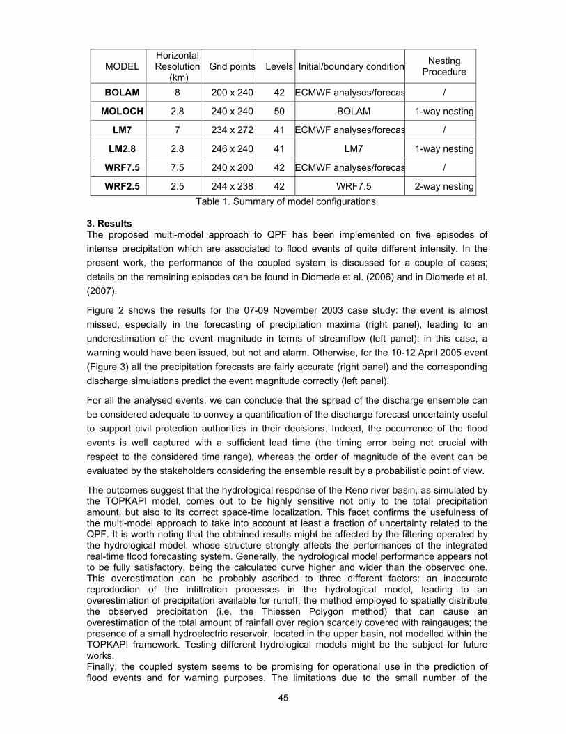
45

MODEL Horizontal Resolution

(km) Grid points Levels Initial/boundary condition Nesting

Procedure

BOLAM 8 200 x 240 42 ECMWF analyses/forecas /

MOLOCH 2.8 240 x 240 50 BOLAM 1-way nesting

LM7 7 234 x 272 41 ECMWF analyses/forecas /

LM2.8 2.8 246 x 240 41 LM7 1-way nesting

WRF7.5 7.5 240 x 200 42 ECMWF analyses/forecas /

WRF2.5 2.5 244 x 238 42 WRF7.5 2-way nestingTable 1. Summary of model configurations.

3. Results The proposed multi-model approach to QPF has been implemented on five episodes of intense precipitation which are associated to flood events of quite different intensity. In the present work, the performance of the coupled system is discussed for a couple of cases; details on the remaining episodes can be found in Diomede et al. (2006) and in Diomede et al. (2007).

Figure 2 shows the results for the 07-09 November 2003 case study: the event is almost missed, especially in the forecasting of precipitation maxima (right panel), leading to an underestimation of the event magnitude in terms of streamflow (left panel): in this case, a warning would have been issued, but not and alarm. Otherwise, for the 10-12 April 2005 event (Figure 3) all the precipitation forecasts are fairly accurate (right panel) and the corresponding discharge simulations predict the event magnitude correctly (left panel).

For all the analysed events, we can conclude that the spread of the discharge ensemble can be considered adequate to convey a quantification of the discharge forecast uncertainty useful to support civil protection authorities in their decisions. Indeed, the occurrence of the flood events is well captured with a sufficient lead time (the timing error being not crucial with respect to the considered time range), whereas the order of magnitude of the event can be evaluated by the stakeholders considering the ensemble result by a probabilistic point of view.

The outcomes suggest that the hydrological response of the Reno river basin, as simulated by the TOPKAPI model, comes out to be highly sensitive not only to the total precipitation amount, but also to its correct space-time localization. This facet confirms the usefulness of the multi-model approach to take into account at least a fraction of uncertainty related to the QPF. It is worth noting that the obtained results might be affected by the filtering operated by the hydrological model, whose structure strongly affects the performances of the integrated real-time flood forecasting system. Generally, the hydrological model performance appears not to be fully satisfactory, being the calculated curve higher and wider than the observed one. This overestimation can be probably ascribed to three different factors: an inaccurate reproduction of the infiltration processes in the hydrological model, leading to an overestimation of precipitation available for runoff; the method employed to spatially distribute the observed precipitation (i.e. the Thiessen Polygon method) that can cause an overestimation of the total amount of rainfall over region scarcely covered with raingauges; the presence of a small hydroelectric reservoir, located in the upper basin, not modelled within the TOPKAPI framework. Testing different hydrological models might be the subject for future works. Finally, the coupled system seems to be promising for operational use in the prediction of flood events and for warning purposes. The limitations due to the small number of the

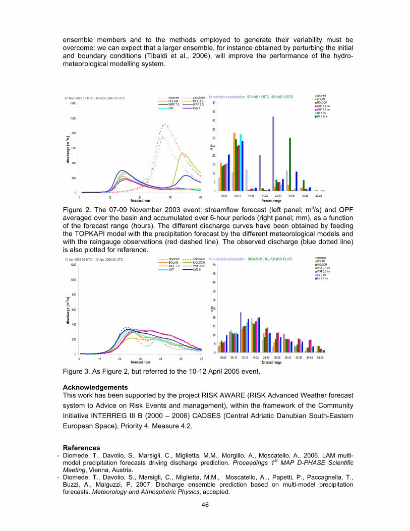
46

ensemble members and to the methods employed to generate their variability must be overcome: we can expect that a larger ensemble, for instance obtained by perturbing the initial and boundary conditions (Tibaldi et al., 2006), will improve the performance of the hydro-meteorological modelling system.

07 Nov 2003 13 UTC - 09 Nov 2003 12 UTC

0

200

400

600

800

1000

1200

0 12 24 36 48forecast hour

disc

harg

e [m

3 /s]

observed calculatedBOLAM MOLOCHWRF 7.5 WRF 2.5LM7 LM2.8

6h cumulative precipitation 07/11/03 13 UTC - 09/11/03 12 UTC

0

5

10

15

20

25

30

35

40

45

50

00-06 06-12 12-18 18-24 24-30 30-36 36-42 42-48forecast range

mm

observedBOLAMMOLOCHWRF 7.5 kmWRF 2.5 kmLM 7 kmLM 2.8 km

Figure 2. The 07-09 November 2003 event: streamflow forecast (left panel; m3/s) and QPF averaged over the basin and accumulated over 6-hour periods (right panel; mm), as a function of the forecast range (hours). The different discharge curves have been obtained by feeding the TOPKAPI model with the precipitation forecast by the different meteorological models and with the raingauge observations (red dashed line). The observed discharge (blue dotted line) is also plotted for reference.

10 Apr 2005 01 UTC - 13 Apr 2005 00 UTC

0

200

400

600

800

1000

1200

0 12 24 36 48 60 72forecast hour

disc

harg

e [m

3 /s]

observed calculatedBOLAM MOLOCHWRF 7.5 WRF 2.5LM7 LM2.8

6h cumulative precipitation 10/04/05 01UTC - 12/04/05 12 UTC

0

5

10

15

20

25

30

35

40

45

50

00-06 06-12 12-18 18-24 24-30 30-36 36-42 42-48 48-54 54-60forecast range

mm

observedBOLAMMOLOCHWRF 7.5 kmWRF 2.5 kmLM 7 kmLM 2.8 km

Figure 3. As Figure 2, but referred to the 10-12 April 2005 event. Acknowledgements This work has been supported by the project RISK AWARE (RISK Advanced Weather forecast system to Advice on Risk Events and management), within the framework of the Community Initiative INTERREG III B (2000 – 2006) CADSES (Central Adriatic Danubian South-Eastern European Space), Priority 4, Measure 4.2.

References

- Diomede, T., Davolio, S., Marsigli, C., Miglietta, M.M., Morgillo, A., Moscatello, A.. 2006. LAM multi-model precipitation forecasts driving discharge prediction. Proceedings 1st MAP D-PHASE Scientific Meeting, Vienna, Austria.

- Diomede, T., Davolio, S., Marsigli, C., Miglietta, M.M., Moscatello, A.., Papetti, P., Paccagnella, T., Buzzi, A., Malguzzi, P. 2007. Discharge ensemble prediction based on multi-model precipitation forecasts. Meteorology and Atmospheric Physics, accepted.

47

- Hamill, T., Clark, M., Schaake, J., Buizza, R. 2005. 2nd HEPEX Workshop Summary Report, Boulder, Colorado (http://hydis8.eng.uci.edu/hepex/scndwksp/HEPEX05-Summary.pdf).

- Krzysztofowicz, R. 1999. Bayesian theory of probabilistic forecasting via deterministic hydrologic model. Water Resources Research, 35 (9), pp.2739-2750.

- Kwadijk, J. 2003. EFFS - European Flood Forecasting System. Final report of Contract EVG1-CT-1999-00011 (http://effs.wldelft.nl).

- Siccardi, F., Boni, G., Ferraris, L.., Rudari, R. 2005. A hydrometeorological approach for probabilistic flood forecast. Journal of Geophysical Research, 110: D05101, doi:10.1029/2004JD005314.

- Tibaldi, S., Paccagnella, T., Marsigli, C., Montani, A., Nerozzi, F. 2006. Limited-Area Ensemble Forecasting: the COSMO-LEPS System. Predictabilty of Weather and Climate, CAMBRIDGE University Press.

- Todini, E., Ciarapica, L. 2001. The TOPKAPI model. In: Mathematical Models of Large Watershed Hydrology, Chapter 12, V.P. Singh. et al. (Eds.), Water Resources Publications.

48

Discharge ensemble forecasts based on the COSMO-LEPS quantitative precipitation by T. Diomede, C. Marisgli, A. Montani and T. Paccagnella

DISCHARGE ENSEMBLE FORECASTS BASED ON THE COSMO-LEPS QUANTITATIVE PRECIPITATION Tommaso Diomede1,2*, Chiara Marsigli1, Andrea Montani1, Tiziana Paccagnella1 1 Regional Hydro-Meteorological Service ARPA-SIM, Bologna, Italy 2 Centro Interuniversitario di Ricerca in Monitoraggio Ambientale (CIMA), Università degli studi di Genova e della Basilicata, Savona, Italy * Corresponding author: Tommaso Diomede, Viale Silvani 6 40122 Bologna Italy, +390516497512, tdiomede@arpa.emr.it Abstract In the present study the usefulness and the skill of the meteorological mesoscale ensemble prediction system COSMO-LEPS is evaluated as a tool to operationally supply quantitative precipitation forecasts driving a meteo-hydrological coupled system aimed at providing reliable real-time discharge ensemble forecasts for the Reno river basin, a medium-size catchment in northern Italy. The hydrological simulations are carried out by means of the distributed rainfall-runoff model TOPKAPI. The performance of the proposed probabilistic forecasting chain is evaluated simulating the streamflow forecasts provided for the autumn seasons of the period 2003-2005. The deterministic forecasting chain, operationally implemented, based on the same rainfall-runoff model fed with the precipitation forecast provided by the COSMO model-suite LAMI is used as term of comparison. 1. Introduction The quantitative precipitation forecast (QPF) is still a challenging task at the scales of interest for hydrological predictions. Although the use of high resolution limited-area models (LAMs) has improved the short-range prediction of locally intense events, it is sometimes difficult to forecast accurately their space-time evolution, especially for ranges longer than 48 hours (Marsigli et al., 2005). Nowadays, the ensemble prediction techniques are widely used in the meteorological community, allowing to add probabilistic information to the forecasts, especially with respect to risk-related events. Moreover, meteorological ensemble systems have recently been used to provide a probabilistic input to hydrological forecasts, in order to improve both the accuracy of these forecasts and the reliability of uncertainty estimates.

In this work, the use of a Limited Ensemble Predictions System (LEPS) is considered as the meteorological contribution to a meteo-hydrological probabilistic forecasting chain. In this way, the estimate of uncertainty affecting hydrological model predictions is related with the problem to integrate meteorological forecast uncertainty into a hydrological model capable to propagate it into hydrological forecast and warning uncertainty.

2. Methodology The proposed probabilistic flood forecasting chain is based on the following tools: - COSMO-LEPS, a Limited-area Ensemble Prediction System based on the non-hydrostatic limited-area model COSMO, daily running (12 UTC) at ECMWF (European Centre for Medium-Range Weather Forecasts) since November 2002; - TOPKAPI (TOPographic Kinematic APproximation and Integration), a physically-based distributed rainfall-runoff model model (Todini and Ciarapica, 2001).

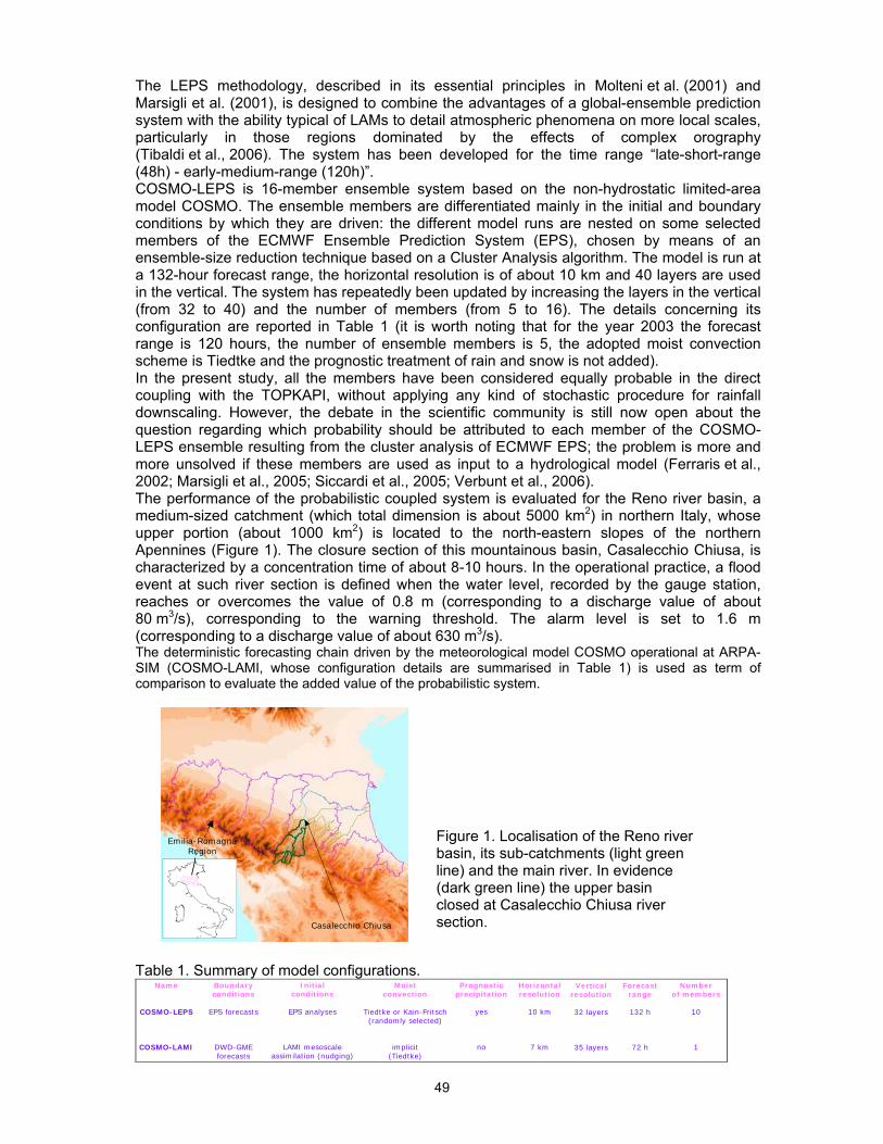
49

The LEPS methodology, described in its essential principles in Molteni et al. (2001) and Marsigli et al. (2001), is designed to combine the advantages of a global-ensemble prediction system with the ability typical of LAMs to detail atmospheric phenomena on more local scales, particularly in those regions dominated by the effects of complex orography (Tibaldi et al., 2006). The system has been developed for the time range “late-short-range (48h) - early-medium-range (120h)”. COSMO-LEPS is 16-member ensemble system based on the non-hydrostatic limited-area model COSMO. The ensemble members are differentiated mainly in the initial and boundary conditions by which they are driven: the different model runs are nested on some selected members of the ECMWF Ensemble Prediction System (EPS), chosen by means of an ensemble-size reduction technique based on a Cluster Analysis algorithm. The model is run at a 132-hour forecast range, the horizontal resolution is of about 10 km and 40 layers are used in the vertical. The system has repeatedly been updated by increasing the layers in the vertical (from 32 to 40) and the number of members (from 5 to 16). The details concerning its configuration are reported in Table 1 (it is worth noting that for the year 2003 the forecast range is 120 hours, the number of ensemble members is 5, the adopted moist convection scheme is Tiedtke and the prognostic treatment of rain and snow is not added). In the present study, all the members have been considered equally probable in the direct coupling with the TOPKAPI, without applying any kind of stochastic procedure for rainfall downscaling. However, the debate in the scientific community is still now open about the question regarding which probability should be attributed to each member of the COSMO-LEPS ensemble resulting from the cluster analysis of ECMWF EPS; the problem is more and more unsolved if these members are used as input to a hydrological model (Ferraris et al., 2002; Marsigli et al., 2005; Siccardi et al., 2005; Verbunt et al., 2006). The performance of the probabilistic coupled system is evaluated for the Reno river basin, a medium-sized catchment (which total dimension is about 5000 km2) in northern Italy, whose upper portion (about 1000 km2) is located to the north-eastern slopes of the northern Apennines (Figure 1). The closure section of this mountainous basin, Casalecchio Chiusa, is characterized by a concentration time of about 8-10 hours. In the operational practice, a flood event at such river section is defined when the water level, recorded by the gauge station, reaches or overcomes the value of 0.8 m (corresponding to a discharge value of about 80 m3/s), corresponding to the warning threshold. The alarm level is set to 1.6 m (corresponding to a discharge value of about 630 m3/s). The deterministic forecasting chain driven by the meteorological model COSMO operational at ARPA-SIM (COSMO-LAMI, whose configuration details are summarised in Table 1) is used as term of comparison to evaluate the added value of the probabilistic system.

Casalecchio Chiusa

Emilia-RomagnaRegion

Figure 1. Localisation of the Reno river basin, its sub-catchments (light green line) and the main river. In evidence (dark green line) the upper basin closed at Casalecchio Chiusa river section.

Table 1. Summary of model configurations.

Name

COSMO-LEPS

COSMO-LAMI

Boundaryconditions

EPS forecasts

DWD-GMEforecasts

Initialconditions

EPS analyses

LAMI mesoscaleassimilation (nudging)

Moistconvection

Tiedtke or Kain-Fritsch(randomly selected)

implicit(Tiedtke)

Prognosticprecipitation

yes

no

Horizontalresolution

10 km

7 km

Verticalresolution

32 layers

35 layers

Forecastrange

132 h

72 h

Numberof members

10

1

50

3. Results Discharge predictions based on the COSMO-LEPS ensemble precipitation forecasts have been computed for the autumn seasons of the years 2003, 2004 and 2005. A statistical analysis, in terms of mean error and root mean squared error, is carried out on the ensemble of hourly discharge forecasts to investigate which quantile is more suitable to represent the ensemble forecast and to compare the performance of the probabilistic approach with the corresponding one provided by the deterministic forecasting chain. From the computations (shown in Figures 2 and 3 only for the autumn 2003) it derives that:

- the 80% and 90% quantiles perform generally better with respect to the ensemble mean as the lead-time increases. This trend is more evident when the autumn season is characterised by higher streamflow values (years 2003 and 2004).

- the performance decay of the probabilistic coupled system is evident up to the first 48-hour forecast range; for higher lead-times, the decay is partly compensated by the ensemble skill.

- the discharge simulations based on the deterministic precipitation forecast perform slightly better for the first 24-hour range. The added value of the probabilistic system comes out in the next forecast ranges.

A further analysis (whose results are not shown) has been carried out about the verification of warnings and alarms based on the predicted discharges:

- for the warning level, the false alarms provided by the higher quantiles (80% and 90%) of the probabilistic forecasting chain do not increase considerably with respect to the ones produced by the deterministic chain, except for the 90% quantile in autumn 2005; on the other hand, if the higher quantiles are considered, the miss events decrease with respect to those obtained with the ensemble mean or the deterministic forecast;

- for the alarm level, if the 90% quantile is considered, no false alarms would have been issued by the probabilistic forecasting chain, whereas one false alarm would have been issued by the deterministic one for a case in autumn 2005; about the miss events, both the forecasting chains fail the forecast of the three events occurred (two in autumn 2003, one in autumn 2004).

Generally, we can conclude that the discharge predictions based on the COSMO-LEPS ensemble precipitation forecasts show performance which are comparable to the single-valued forecast driven by COSMO-LAMI for the first 24-hour forecast range. The added value of the probabilistic system comes out with increasing lead-times, especially starting from the +48-72 forecast range. The timing of the streamflow simulations driven by COSMO-LEPS matches quite well the event occurrence and the number of false alarms is limited, also with the lead-time increasing. On the other hand, the prediction of the event magnitude is less accurate, especially for the higher streamflows, usually underestimated.

The next developments will be addressed to evaluate the system performance in other seasons and the impact of tagging each member with a probability measure representing the relative size of the cluster resulting from the cluster analysis of ECMWF EPS.

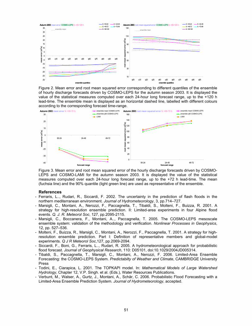
51

Autumn 2003 mean error COSMO-LEPS fc +00-120 h

-30

-25

-20

-15

-10

-5

0

5

10

15

20

25

30

35

q05 q10 q20 q25 q40 q50 q60 q75 q80 q90 q95

ensemble quantiles

mea

n er

ror (

m3 /s

)

fc +00-24 fc +24-48fc +48-72 fc +72-96fc +96-120_ _ _ _ ensemble mean

Autumn 2003 root mean squared error COSMO-LEPS fc +00-120 h

10

30

50

70

90

110

130

q05 q10 q20 q25 q40 q50 q60 q75 q80 q90 q95ensemble quantiles

root

mea

n sq

uare

d er

ror (

m3 /s

)

fc +00-24 fc +24-48fc +48-72 fc +72-96fc +96-120_ _ _ _ ensemble mean

Figure 2. Mean error and root mean squared error corresponding to different quantiles of the ensemble of hourly discharge forecasts driven by COSMO-LEPS for the autumn season 2003. It is displayed the value of the statistical measures computed over each 24-hour long forecast range, up to the +120 h lead-time. The ensemble mean is displayed as an horizontal dashed line, labelled with different colours according to the corresponding forecast time-range. Autumn 2003 mean error fc +00-72 h

-40

-30

-20

-10

0

10

20

30

00-24 24-48 48-72

forecast range

mea

n er

ror (

m3 /s

)

ensemble mean COSMO-LEPSensemble q90 COSMO-LEPSLAMI

Autumn 2003 root mean squared error fc +00-72 h

0

20

40

60

80

100

120

140

160

00-24 24-48 48-72forecast range

root

mea

n sq

uare

d er

ror (

m3 /s

)

ensemble mean COSMO-LEPS

ensemble q90 COSMO-LEPSLAMI

Figure 3. Mean error and root mean squared error of the hourly discharge forecasts driven by COSMO-LEPS and COSMO-LAMI for the autumn season 2003. It is displayed the value of the statistical measures computed over each 24-hour long forecast range, up to the +72 h lead-time. The mean (fuchsia line) and the 90% quantile (light green line) are used as representative of the ensemble. References

- Ferraris, L.., Rudari, R., Siccardi, F. 2002. The uncertainty in the prediction of flash floods in the northern mediterranean environment. Journal of Hydrometeorology, 3, pp.714–727.

- Marsigli, C., Montani, A., Nerozzi, F., Paccagnella, T., Tibaldi, S., Molteni, F., Buizza, R. 2001. A strategy for high-resolution ensemble prediction. II: Limited-area experiments in four Alpine flood events. Q. J. R. Meteorol Soc, 127, pp.2095-2115.

- Marsigli, C., Boccanera, F., Montani, A.., Paccagnella, T. 2005. The COSMO-LEPS mesoscale ensemble system: validation of the methodology and verification. Nonlinear Processes in Geophysics, 12, pp. 527–536.

- Molteni, F., Buizza, R., Marsigli, C., Montani, A., Nerozzi, F., Paccagnella, T. 2001. A strategy for high-resolution ensemble prediction. Part I: Definition of representative members and global-model experiments. Q J R Meteorol Soc,127, pp.2069-2094.

- Siccardi, F., Boni, G., Ferraris, L.., Rudari, R. 2005. A hydrometeorological approach for probabilistic flood forecast. Journal of Geophysical Research, 110: D05101, doi:10.1029/2004JD005314.

- Tibaldi, S., Paccagnella, T., Marsigli, C., Montani, A., Nerozzi, F. 2006. Limited-Area Ensemble Forecasting: the COSMO-LEPS System. Predictabilty of Weather and Climate, CAMBRIDGE University Press

- Todini, E., Ciarapica, L. 2001. The TOPKAPI model. In: Mathematical Models of Large Watershed Hydrology, Chapter 12, V.P. Singh. et al. (Eds.), Water Resources Publications.

- Verbunt, M., Walser, A., Gurtz, J., Montani, A., Schär, C. 2006. Probabilistic Flood Forecasting with a Limited-Area Ensemble Prediction System. Journal of Hydrometeorology, accepted.

52

E-F

Status of the Great Lakes Testbed project by V. Fortin and A. Pietroniro

STATUS OF THE GREAT LAKES TESTBED PROJECT Vincent Fortin1* and Alain Pietroniro2 1 Meteorological Research Division, Environment Canada 2 Aquatic Ecosystem Impacts Research Division, Environment Canada * Corresponding author: Canadian Meteorological Centre, 2121 Trans-Canada Highway, 5th floor, Dorval (Québec) Canada H9P 1J3, 1(514)421-4630, vincent.fortin@ec.gc.ca Abstract The Great Lakes and St. Lawrence testbed project aims to demonstrate the importance of detailed atmospheric and hydrologic modeling for medium-range atmospheric and hydrologic forecasting on large basins. During the past two years, efforts have been focused on the implementation and verification of the regional, raster-based, MESH surface and hydrological model which is coupled to the global Canadian ensemble prediction system to obtain ensemble forecasts of land-surface variables as well as streamflow on the basin. This system will serve as a baseline to test if we can manage to improve the performance of the system by either increasing the horizontal resolution of the surface model, downscaling the ensemble forecasts using a limited-area model, or improve the parameterization of surface and sub-surface processes. In time, this should lead us to recommend a setup which maximizes the quality of hydrological forecasts for a given cost in terms of computer resources, and also point out what are the weakest links of the ensemble hydrological forecasting chain, so that efforts can be focused on these components. Meanwhile, the forecasts from the baseline forecasting system can be analyzed by end-users, helping researchers and forecasters to develop products that are useful for water management, by getting feedback on actual ensemble forecasts of future events. In this presentation, we assess the strengths and weaknesses of the forecasting system and discuss how we propose to improve it in the coming years through collaboration with researchers and stakeholders who have manifested interest in the Great Lakes testbed project.

53

Short-term streamflow prediction for a small midwestern watershed by K. J. Franz, W. A. Gallus, M. Baker, K.A. Jungbluth and W. S. Lincoln

SHORT-TERM STREAMFLOW PREDICTION FOR A SMALL MIDWESTERN WATERSHED Kristie J. Franz1*, William A. Gallus, Jr.1, Marian Baker2, Karl A. Jungbluth2, and W. Scott Lincoln1

1.Department of Geological and Atmospheric Sciences, Iowa State University, Ames, IA 2.WFO Des Moines (DMX), US National Weather Service, National Oceanic and Atmospheric Administration, Johnston, IA *Corresponding Author: Kristie Franz, Iowa State University, Dept. of Geological and Atmospheric Sciences, 3023 Agronomy Hall, Ames, IA 50011, kfranz@iastate.edu, 515-294-7454 ABSTRACT In this paper, a cooperative investigation undertaken by researchers at Iowa State University and forecasters at the Des Moines Weather Forecast Office (DMX) is presented. The purpose of the study is to examine the use of both a proposed hydrologic forecast model and meteorological predictions for flood forecasting in small watersheds. Current U.S. National Weather Service (NWS) flash flood prediction methods are based on guidance that is generated in a one-time step and is seldom updated. Predictions out to several days are generated using the Sacramento Soil Moisture Accounting model (SACSMA), which is most commonly applied at a 6-hour simulation time step. The 6-hour time step is inadequate for small watersheds with a short response time. The city of Ames, Iowa, for example, generates their own predictions using the U.S. Army Corps HEC-Hydrologic Modeling System (HEC-HMS) because they found that the six-hour simulations of the NWS did not meet their basin-specific flood forecasting needs. Given this apparent successful application of the HEC-HMS, the feasibility of implementing the model for operational short-term streamflow prediction at the DMX will be tested. The Ames watershed will be used as an initial test site. This study will also examine the possibility of using 1-hour quantitative precipitation forecasts (QPF) and 1-hour probabilistic QPF (PQPF) to provide early indications of flood potential in combination with the HEC-HMS and SACSMA. Observed precipitation is the primary variable currently used in flood prediction. Therefore, the lead time of flood warnings are dependent upon the rate of data collection and download, the time to initiate and run the model, the location of the precipitation, and basin response time. However, additional lead time may be gained through the use of quantitative precipitation forecasts (QPFs). QPFs are not commonly used in an objective manner for flash flood prediction by the DMX. Two major challenges facing the DMX flood forecasting operations are addressed: (1) the application of hydrologic models at time steps less than 6 hours for flash flood prediction in small watersheds, and (2) the objective use of quantitative precipitation forecasts (both deterministic and ensemble) to improve flood forecast lead time. Successful demonstration of the HEC-HMS and/or QPFs will provide opportunities for wider application within the DMX and other WFO districts.

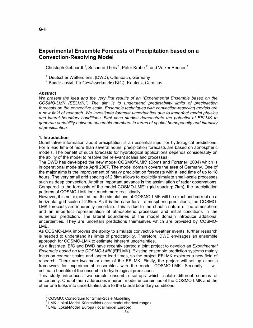
54

G-H

Experimental Ensemble Forecasts of Precipitation based on a Convection-Resolving Model by C. Gebhardt, S.Theis, P. Krahe, and V. Renner

Experimental Ensemble Forecasts of Precipitation based on a Convection-Resolving Model

Christoph Gebhardt 1, Susanne Theis 1, Peter Krahe 2, and Volker Renner 1

1 Deutscher Wetterdienst (DWD), Offenbach, Germany 2 Bundesanstalt für Gewässerkunde (BfG), Koblenz, Germany

Abstract We present the idea and the very first results of an “Experimental Ensemble based on the COSMO-LMK (EELMK)”. The aim is to understand predictability limits of precipitation forecasts on the convective scale. Ensemble techniques with convection-resolving models are a new field of research. We investigate forecast uncertainties due to imperfect model physics and lateral boundary conditions. First case studies demonstrate the potential of EELMK to generate variability between ensemble members in terms of spatial homogeneity and intensity of precipitation. 1. Introduction Quantitative information about precipitation is an essential input for hydrological predictions. For a lead time of more than several hours, precipitation forecasts are based on atmospheric models. The benefit of such forecasts for hydrological applications depends considerably on the ability of the model to resolve the relevant scales and processes. The DWD has developed the new model COSMO2-LMK3 (Doms and Förstner, 2004) which is in operational mode since April 2007. The model domain covers the area of Germany. One of the major aims is the improvement of heavy precipitation forecasts with a lead time of up to 18 hours. The very small grid spacing of 2.8km allows to explicitly simulate small-scale processes such as deep convection. Another important advance is the assimilation of radar observations. Compared to the forecasts of the model COSMO-LME4 (grid spacing: 7km), the precipitation patterns of COSMO-LMK look much more realistically. However, it is not expected that the simulations of COSMO-LMK will be exact and correct on a horizontal grid scale of 2.8km. As it is the case for all atmospheric predictions, the COSMO-LMK forecasts are inherently uncertain. This is due to the chaotic nature of the atmosphere and an imperfect representation of atmospheric processes and initial conditions in the numerical prediction. The lateral boundaries of the model domain introduce additional uncertainties. They are uncertain predictions themselves which are provided by COSMO-LME. As COSMO-LMK improves the ability to simulate convective weather events, further research is needed to understand its limits of predictability. Therefore, DWD envisages an ensemble approach for COSMO-LMK to estimate inherent uncertainties. As a first step, BfG and DWD have recently started a joint project to develop an Experimental Ensemble based on the COSMO-LMK (EELMK). Existing ensemble prediction systems mainly focus on coarser scales and longer lead times, so the project EELMK explores a new field of research. There are two major aims of the EELMK. Firstly, the project will set up a basic framework for experimental ensembles with the model COSMO-LMK. Secondly, it will estimate benefits of the ensemble to hydrological predictions. This study introduces two simple ensemble set-ups which isolate different sources of uncertainty. One of them addresses inherent model uncertainties of the COSMO-LMK and the other one looks into uncertainties due to the lateral boundary conditions.

2 COSMO: Consortium for Small-Scale Modelling 3 LMK: Lokal-Modell Kürzestfrist (local model shortest-range) 4 LME: Lokal-Modell Europa (local model Europe)

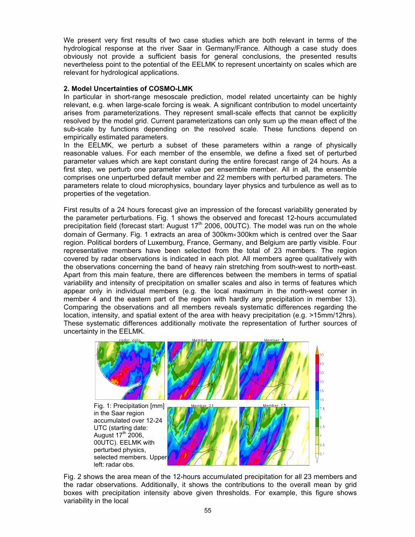
55

We present very first results of two case studies which are both relevant in terms of the hydrological response at the river Saar in Germany/France. Although a case study does obviously not provide a sufficient basis for general conclusions, the presented results nevertheless point to the potential of the EELMK to represent uncertainty on scales which are relevant for hydrological applications. 2. Model Uncertainties of COSMO-LMK In particular in short-range mesoscale prediction, model related uncertainty can be highly relevant, e.g. when large-scale forcing is weak. A significant contribution to model uncertainty arises from parameterizations. They represent small-scale effects that cannot be explicitly resolved by the model grid. Current parameterizations can only sum up the mean effect of the sub-scale by functions depending on the resolved scale. These functions depend on empirically estimated parameters. In the EELMK, we perturb a subset of these parameters within a range of physically reasonable values. For each member of the ensemble, we define a fixed set of perturbed parameter values which are kept constant during the entire forecast range of 24 hours. As a first step, we perturb one parameter value per ensemble member. All in all, the ensemble comprises one unperturbed default member and 22 members with perturbed parameters. The parameters relate to cloud microphysics, boundary layer physics and turbulence as well as to properties of the vegetation. First results of a 24 hours forecast give an impression of the forecast variability generated by the parameter perturbations. Fig. 1 shows the observed and forecast 12-hours accumulated precipitation field (forecast start: August 17th 2006, 00UTC). The model was run on the whole domain of Germany. Fig. 1 extracts an area of 300km×300km which is centred over the Saar region. Political borders of Luxemburg, France, Germany, and Belgium are partly visible. Four representative members have been selected from the total of 23 members. The region covered by radar observations is indicated in each plot. All members agree qualitatively with the observations concerning the band of heavy rain stretching from south-west to north-east. Apart from this main feature, there are differences between the members in terms of spatial variability and intensity of precipitation on smaller scales and also in terms of features which appear only in individual members (e.g. the local maximum in the north-west corner in member 4 and the eastern part of the region with hardly any precipitation in member 13). Comparing the observations and all members reveals systematic differences regarding the location, intensity, and spatial extent of the area with heavy precipitation (e.g. >15mm/12hrs). These systematic differences additionally motivate the representation of further sources of uncertainty in the EELMK. Fig. 2 shows the area mean of the 12-hours accumulated precipitation for all 23 members and the radar observations. Additionally, it shows the contributions to the overall mean by grid boxes with precipitation intensity above given thresholds. For example, this figure shows variability in the local

Fig. 1: Precipitation [mm] in the Saar region accumulated over 12-24 UTC (starting date: August 17th 2006, 00UTC). EELMK with perturbed physics, selected members. Upper left: radar obs.

56

Figure 2: Area mean of precipitation [mm] in the Saar region accumulated over 12-24 UTC (starting date: August 17th 2006, 00UTC). Based on the EELMK with perturbed physics (member 1 is unperturbed). rain intensity among the members independently of the overall mean (e.g. members 4 and 5). Again, there are obvious systematic differences between the EELMK and the observations. 3. Uncertainty due to Lateral Boundary Conditions In the operational set-up at DWD, the COSMO-LMK is nested into forecasts of the regional model COSMO-LME (7km grid spacing) which provides lateral boundary conditions to COSMO-LMK. Depending on the large-scale flow, these lateral boundary conditions exert a noticeable influence on the COSMO-LMK forecast. They can induce a considerable amount of uncertainty to the COSMO-LMK forecast and consequently for the hydrological application. A promising strategy to represent the uncertainty of the boundary conditions is the generation of a sequence of ensembles which leads from a global EPS to a regional EPS and finally to the EELMK. As a first experiment, we have nested the EELMK into ensemble members of COSMO-SREPS (COSMO Short Range Ensemble Prediction System). The COSMO-SREPS is a regional EPS on the basis of the model COSMO-LM with 10 km grid spacing. It is designed for forecast lead times of up to 2-3 days. COSMO-SREPS is under development at ARPA-SIM in Bologna, Italy. COSMO-SREPS itself is nested into a multi-model EPS which is developed at Instituto Nacional Meteorologia (INM) in Madrid, Spain. The COSMO-SREPS comprises 16 ensemble members which can be categorized into four groups of four members. Each group is linked to a different global model (IFS, GME, NCEP, UKMO). Each of the four members within a group pertains to one of four different physics perturbations in the COSMO-LM. We have run a first case study with 16 members, each of which is nested in one of the COSMO-SREPS members but with unperturbed COSMO-LMK physics. The forecast starts on September 17th 2006, 00UTC, and covers 24 hours. Fig. 3 shows the observed and forecast 12-hours accumulated precipitation field for the Saar region (forecast start: September 17th 2006 00UTC). Each of the selected members is associated with one of the global models used in the INM ensemble. Within the EELMK, the main precipitation feature is similar in all members. Its location and spatial extent, however, clearly depend on the global model. Compared to the observations, all forecasts can be considered as valuable on the broad scale, but there are discrepancies in spatial homogeneity and intensity.

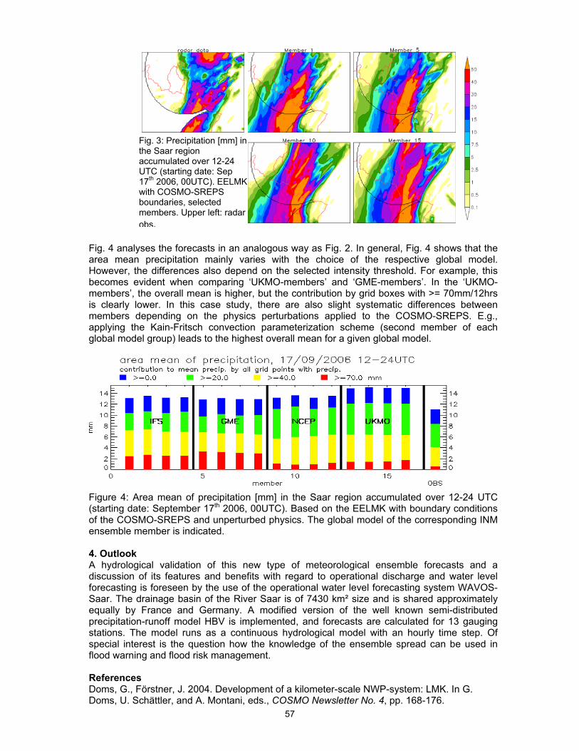
57

Fig. 4 analyses the forecasts in an analogous way as Fig. 2. In general, Fig. 4 shows that the area mean precipitation mainly varies with the choice of the respective global model. However, the differences also depend on the selected intensity threshold. For example, this becomes evident when comparing ‘UKMO-members’ and ‘GME-members’. In the ‘UKMO-members’, the overall mean is higher, but the contribution by grid boxes with >= 70mm/12hrs is clearly lower. In this case study, there are also slight systematic differences between members depending on the physics perturbations applied to the COSMO-SREPS. E.g., applying the Kain-Fritsch convection parameterization scheme (second member of each global model group) leads to the highest overall mean for a given global model.

Figure 4: Area mean of precipitation [mm] in the Saar region accumulated over 12-24 UTC (starting date: September 17th 2006, 00UTC). Based on the EELMK with boundary conditions of the COSMO-SREPS and unperturbed physics. The global model of the corresponding INM ensemble member is indicated. 4. Outlook A hydrological validation of this new type of meteorological ensemble forecasts and a discussion of its features and benefits with regard to operational discharge and water level forecasting is foreseen by the use of the operational water level forecasting system WAVOS-Saar. The drainage basin of the River Saar is of 7430 km² size and is shared approximately equally by France and Germany. A modified version of the well known semi-distributed precipitation-runoff model HBV is implemented, and forecasts are calculated for 13 gauging stations. The model runs as a continuous hydrological model with an hourly time step. Of special interest is the question how the knowledge of the ensemble spread can be used in flood warning and flood risk management. References Doms, G., Förstner, J. 2004. Development of a kilometer-scale NWP-system: LMK. In G. Doms, U. Schättler, and A. Montani, eds., COSMO Newsletter No. 4, pp. 168-176.

Fig. 3: Precipitation [mm] in the Saar region accumulated over 12-24 UTC (starting date: Sep 17th 2006, 00UTC). EELMK with COSMO-SREPS boundaries, selected members. Upper left: radar obs.

58

Hydrological ensemble prediction systems: the 1966 century flood experiment by G. Grossi, B. Bacchi, R. Buizza and R. Ranzi

Hydrological Ensemble Prediction Systems: the 1966 “century” flood experiment G. Grossi1*, B. Bacchi1, R. Buizza2 and R. Ranzi1

1DICATA, University of Brescia, Italy 2ECMWF, Reading, UK *Corresponding author: Giovanna Grossi, DICATA, Università di Brescia, via Branze 43 – 25123 BRESCIA, 0039+030+3711294, giovanna.grossi@unibs.it Abstract In order to assess the potential value of hydrological models forced by single and probabilistic weather predictions, a widespread flood event that affected Italy in 1966 has been revisited with state-of-the-art models. First, a complete single-forecast model chain consisting of the ECMWF global model, forcing in cascade two meso-scale models and a hydrological model, was applied to predict precipitation and the associated hydrological aspects in North-eastern Italy (Adige river basin and adjacent basins) and Central Italy (Arno river basin). Since these first sets of results based on single forecasts indicate that simulated precipitation patterns are in general very sensitive to initial conditions, the case has been analyzed using an ensemble approach. Hydrological ensemble forecasts are now being generated in order to i) investigate the relative contribution of meso-scale models to predict the driving meteorological fields, and ii) assess the sensitivity of forecast quality to ensemble size. For this latter point, a methodology that could be used to identify few ‘key’ members of the ECMWF ensemble to be downscaled through a meso-scale model before they are used to force the hydrological model is investigated: such a procedure could be used in an operational framework to reduce the resources required to generate hydrological ensemble forecasts. 1. Introduction The Institute of Atmospheric Sciences and Climate of the Italian National Resource Council (ISAC-CNR), the University of Brescia and the European Centre for Medium-Range Weather Forecasts (ECMWF) have been working together to revisit a severe weather and flood event that caused huge damages and loss of lives in Central and North-Eastern Italy at the beginning of November 1966 (Flood66 – see Figure 1). The cities of Florence, Trento and Venice were seriously damaged by the Flood66 event. The main goal of this collaboration has been to assess the potential value of HEPS (Hydrological Ensemble Prediction Systems; Schaake et al 2007), based on state-of-the-art numerical meteorological and hydrological models, in estimating the variance of some important flood indexes (such as the time to peak, the peak flood, volumes, etc.) induced by forecast rainfall variability. The ECMWF data used for this study consist of TL511L61 (spectral triangular truncation 511 with liner grid, and 61 vertical levels) resolution reanalyses and single forecasts, and TL399L40 ensemble forecasts valid for a period covering the end of October and the beginning of November 1966. Reanalyses, single high-resolution and ensemble forecasts for the last days of the simulated period have been used to define the initial and boundary conditions to generate the BOLAM (limited area, hydrostatic) and MOLOCH (non hydrostatic) meso-scale model forecasts (Malguzzi et al., 2006). Meteorological and hydrological forecasts have been compared to observed rain-gauge precipitation data and runoff hydrographs collected for the two study areas.

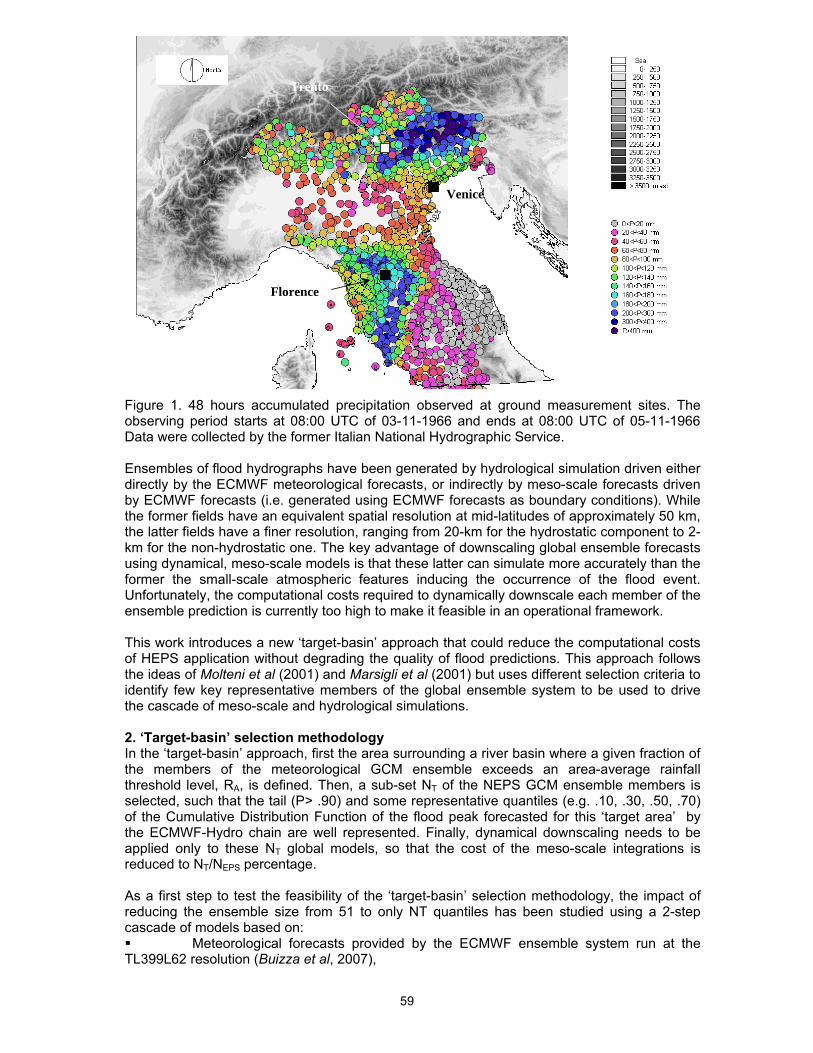
59

Figure 1. 48 hours accumulated precipitation observed at ground measurement sites. The observing period starts at 08:00 UTC of 03-11-1966 and ends at 08:00 UTC of 05-11-1966 Data were collected by the former Italian National Hydrographic Service. Ensembles of flood hydrographs have been generated by hydrological simulation driven either directly by the ECMWF meteorological forecasts, or indirectly by meso-scale forecasts driven by ECMWF forecasts (i.e. generated using ECMWF forecasts as boundary conditions). While the former fields have an equivalent spatial resolution at mid-latitudes of approximately 50 km, the latter fields have a finer resolution, ranging from 20-km for the hydrostatic component to 2-km for the non-hydrostatic one. The key advantage of downscaling global ensemble forecasts using dynamical, meso-scale models is that these latter can simulate more accurately than the former the small-scale atmospheric features inducing the occurrence of the flood event. Unfortunately, the computational costs required to dynamically downscale each member of the ensemble prediction is currently too high to make it feasible in an operational framework. This work introduces a new ‘target-basin’ approach that could reduce the computational costs of HEPS application without degrading the quality of flood predictions. This approach follows the ideas of Molteni et al (2001) and Marsigli et al (2001) but uses different selection criteria to identify few key representative members of the global ensemble system to be used to drive the cascade of meso-scale and hydrological simulations. 2. ‘Target-basin’ selection methodology In the ‘target-basin’ approach, first the area surrounding a river basin where a given fraction of the members of the meteorological GCM ensemble exceeds an area-average rainfall threshold level, RA, is defined. Then, a sub-set NT of the NEPS GCM ensemble members is selected, such that the tail (P> .90) and some representative quantiles (e.g. .10, .30, .50, .70) of the Cumulative Distribution Function of the flood peak forecasted for this ‘target area’ by the ECMWF-Hydro chain are well represented. Finally, dynamical downscaling needs to be applied only to these NT global models, so that the cost of the meso-scale integrations is reduced to NT/NEPS percentage. As a first step to test the feasibility of the ‘target-basin’ selection methodology, the impact of reducing the ensemble size from 51 to only NT quantiles has been studied using a 2-step cascade of models based on: Meteorological forecasts provided by the ECMWF ensemble system run at the

TL399L62 resolution (Buizza et al, 2007),

Florence

Venice

Trento

60

Hydrological forecasts nested directly into the ECMWF ensemble forecasts using an event scale hydrological model 3. Preliminary results The target basin methodology has been applied to ensemble forecast starting on the 3rd of November and valid for the 4th-5th November 1966 (the peak discharge of the Arno river and its tributaries was observed in Florence in the morning of the 4th). Two target basins have been considered: the Sieve river basin at the section of Fornacina (829 km2) and the Cellina river basin at the section of Barcis (392 km2): the first watershed is a sub-basin of the Arno river basin, located in the Tuscany area, while the second watershed is located in the Alps, close to the Adige river basin. When the EPS is used to force directly the hydrological model the timing of the forecasted hydrograph is still good, but the peak discharge is underestimated, especially for the Sieve river, but the same weakness can be noticed also for the Cellina river. The rainfall underestimation can be seen by comparing the spread of the area-average precipitation predicted by the ECMWF EPS members, as well as the spread of the HEPS flood volumes: values for the Arno basin, where convective precipitation was dominant, are higher than over the Alps (Figure 2). This precipitation underestimation can be partly due to the coarse resolution of the precipitation field used to force the hydrological model and it suggests the use of a complete model chain, where the precipitation field predicted at the global scale is downscaled by a limited area model before it is used to force the hydrological model. In this preliminary analysis the 48-hour accumulated rainfall (from t=0 to t+48h) was averaged over an area of about 26000 km2, which includes the Arno river basin in Tuscany and several basins in North-Eastern Italy. The spatial average was performed on the most affected river basins, which is where the precipitation forcing was predicted to be more intense. Ensemble members # 37, 3, 33, 16, 19 provide accumulated precipitation values corresponding to the 10%, 30%, 50%, 70% and 90% quantiles, respectively (i.e. 123, 137, 143, 151 and 160 mm respectively) The rainfall temporal distribution and the corresponding flood hydrographs produced using these members only for the Sieve river basin at Fornacina and by the Cellina river basin at Barcis are shown in Figure 3. The comparison of Figs. 2 and 3 indicate that the spread in the peak discharge values is well represented even by the subset of the ensemble predictions. For the Sieve river a peak discharge of 630 m3/s is predicted by member #3, while 861 m3/s would have been predicted by member #5. For the Cellina river member # 19 leads to a peak discharge estimate of 1167 m3/s, while the maximum value for the peak discharge, 1246 m3/s would have been obtained with member #31. In both cases the difference is very low. 4. Conclusions and future plans A new ‘target-basin’ approach has been introduced to extract key, large-scale meteorological information from a global ensemble systems, to be used to drive a cascade of limited-area meso-scale and hydrological models. This approach has been applied to forecasts re-run for a period in November 1966 during which Central and Northern-Eastern Italy, including the historical cities of Florence and Venice, were affected by sever flooding. Preliminary results of the ‘target basin’ approach based on one case are encouraging. They indicate that the members identified by the target-basin approach contain most of the large-scale meteorological information needed to drive the cascade of higher-resolution and hydrological models.

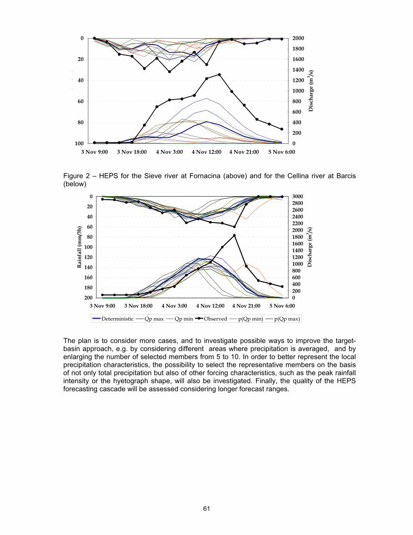
61

0

20

40

60

80

1003 Nov 9:00 3 Nov 18:00 4 Nov 3:00 4 Nov 12:00 4 Nov 21:00 5 Nov 6:00

(/

)

0

200

400

600

800

1000

1200

1400

1600

1800

2000

Dis

char

ge (m

3 /s)

Figure 2 – HEPS for the Sieve river at Fornacina (above) and for the Cellina river at Barcis (below)

The plan is to consider more cases, and to investigate possible ways to improve the target-basin approach, e.g. by considering different areas where precipitation is averaged, and by enlarging the number of selected members from 5 to 10. In order to better represent the local precipitation characteristics, the possibility to select the representative members on the basis of not only total precipitation but also of other forcing characteristics, such as the peak rainfall intensity or the hyetograph shape, will also be investigated. Finally, the quality of the HEPS forecasting cascade will be assessed considering longer forecast ranges.

0

20

40

60

80

100

120

140

160

180

2003 Nov 9:00 3 Nov 18:00 4 Nov 3:00 4 Nov 12:00 4 Nov 21:00 5 Nov 6:00

Rai

nfal

l (m

m/3

h)

020040060080010001200140016001800200022002400260028003000

Dis

char

ge (m

3 /s)

Deterministic Qp max Qp min Observed p(Qp min) p(Qp max)

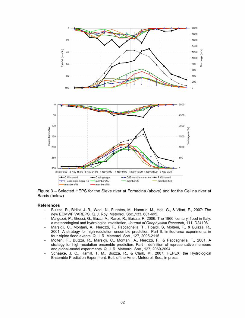
62

Figure 3 – Selected HEPS for the Sieve river at Fornacina (above) and for the Cellina river at Barcis (below) References

- Buizza, R., Bidlot, J.-R., Wedi, N., Fuentes, M., Hamrud, M., Holt, G., & Vitart, F., 2007: The new ECMWF VAREPS. Q. J. Roy. Meteorol. Soc.,133, 681-695.

- Malguzzi, P., Grossi, G., Buzzi, A., Ranzi, R., Buizza, R. 2006. The 1966 ‘century’ flood in Italy: a meteorological and hydrological revisitation, Journal of Geophysical Research, 111, D24106.

- Marsigli, C., Montani, A., Nerozzi, F., Paccagnella, T., Tibaldi, S, Molteni, F., & Buizza, R., 2001. A strategy for high-resolution ensemble prediction. Part II: limited-area experiments in four Alpine flood events. Q. J. R. Meteorol. Soc., 127, 2095-2115.

- Molteni, F., Buizza, R., Marsigli, C., Montani, A., Nerozzi, F., & Paccagnella, T., 2001. A strategy for high-resolution ensemble prediction. Part I: definition of representative members and global-model experiments. Q. J. R. Meteorol. Soc., 127, 2069-2094.

- Schaake, J. C., Hamill, T. M., Buizza, R., & Clark, M., 2007: HEPEX, the Hydrological Ensemble Prediction Experiment. Bull. of the Amer. Meteorol. Soc., in press.

0

20

40

60

80

100

Rai

nfal

l (m

m/3

h)

0

200

400

600

800

1000

1200

1400

1600

1800

2000

Dis

char

ge (m

³/s)

0

50

100

150

200

250

3003 Nov 9:00 3 Nov 15:00 3 Nov 21:00 4 Nov 3:00 4 Nov 9:00 4 Nov 15:00 4 Nov 21:00 5 Nov 3:00

Rai

nfal

l (m

m/3

h)

0

500

1000

1500

2000

2500

3000

Dis

char

ge (m

³/s)

Q Observed Q raingauges Q Ensemble mean +-s P ObservedP Ensemble mean +-s member #37 member #3 member #33member #16 member #19

63

Moving toward operational hydrologic ensemble forecasts by R.K. Hartman

MOVING TOWARD OPERATIONAL HYDROLOGIC ENSEMBLE FORECASTS Robert K. Hartman, Hydrologist in Charge USA/NOAA’s National Weather Service California-Nevada River Forecast Center, Sacramento, CA In the United States, NOAA’s National Weather Service (NWS) has used ensemble stream flow techniques for over twenty years to produce long-range seasonal predictions of unregulated steamflows. These have been more successful in mountainous regions in the West where the snow pack and information about it has a significant impact on spring and summer streamflows. More recently, the potential for short to medium range ensemble streamflow products to serve risk-based decision making for the emergency services, environmental, water management, hydroelectric, and recreational sectors has gained appropriate attention. The process of generating reliable ensembles of stream flow that spans all time scales is complex and challenging. This presentation will cover efforts to date, lessons learned, and known challenges as well as an overview of the Experimental Ensemble Forecasting System (XEFS) which is currently under design for development and operational implementation at NWS River Forecast Centers within the next two to three years.

64

Addressing parameter uncertainty in regional forecast basins using similarity indices by T. Hogue, S. Lopez, K. Franz and J. Barco

ADDRESSING PARAMETER UNCERTAINTY IN REGIONAL FORECAST BASINS USING SIMILARITY INDICES Terri S. Hogue1, Sonya Lopez1, Kristie Franz2 and Janet Barco1

1Department of Civil and Environmental Engineering, University of California Los Angeles 2Department of Geological and Atmospheric Sciences, Iowa State University Abstract Identification of appropriate parameter sets for simulation of streamflow in ungauged basins has become a significant challenge for both operational and research hydrologists. This is especially difficult when using conceptual models, as parameters typically must be “calibrated” or adjusted to match streamflow conditions in specific systems (i.e. some of the parameters are not directly observable). This paper addresses the uncertainty associated with transferring and applying parameters between basins within large-scale regions using conceptual rainfall-runoff models. We use the National Weather Service’s (NWS) operational hydrologic model, the SACramento Soil Moisture Accounting (SAC-SMA) model. The Multi-Step Automatic Calibration Scheme (MACS) (Hogue et al., 2000; 2006) is used to optimize SAC-SMA parameters for watersheds with extensive hydrologic records from the Model Parameter Estimation Experiment (MOPEX) database. MOPEX was established to advance the state of knowledge of parameter estimation techniques and provide guidance on improving a priori estimates of land surface and hydrologic models. We develop a similarity index method (SIM) to establish a range of parameters for a specific hydroclimatic region using NWS-MOPEX forecast basins in the southeastern United States. Indices are based on the physical and hydroclimatic characteristics of the area and are used to develop a “range of parameters” which can be reasonably transferred to similar basins and which represent the associated parameter uncertainty for the region. The impact of regionalized parameters is also evaluated via generation of hindcasts and probabilistic verification procedures (Franz et al., 2003). Hindcasts are used to assess the efficacy of site specific model calibration versus SIM on streamflow forecast skill. References

- Franz, K. J., H. C. Hartmann, S. Sorooshian and R. Bales, 2003: Verification of National Weather Service Ensemble Streamflow Predictions for Water Supply Forecasting in the Colorado River Basin, Journal of Hydrometeorology, 14, 105-1118.

- Hogue, T.S., S. Sorooshian, H. Gupta, A. Holz, and D. Braatz, 2000: A Multi-step Automatic

Calibration Scheme for River Forecasting Models, Journal of Hydrometeorology, 1, 524-542.

- Hogue, T.S., H.V. Gupta, and S. Sorooshian, 2006: A “User-Friendly” Approach to Parameter Estimation in Hydrologic Models, Journal of Hydrology, 320, 202–217.

65

Ensemble streamflow forecasting with the coupled GFS-NOAH modeling system by D. Hou, K. Mitchell, Z. Toth, D. Lohmann and H. Wei

ENSEMBLE STREAMFLOW FORECASTING WITH THE COUPLED GFS-NOAH MODELING SYSTEM Dingchen Hou1*, Kenneth Mitchell2, Zoltan Toth2, Dag Lohmann3 and Helin Wei1 1 Environmental Modeling Center/NCEP/NOAA and SAIC, Camp Springs, USA 2 Environmental Modeling Center/NCEP/NOAA, Camp Springs. USA 3 Risk Management Solution, Ltd., UK * Corresponding author: Dingchen Hou, W/NP2, NOAA, WWB #207, 5200 Auth Road, MD 20746, U.S.A. Phone: (301)7638000; Email:dingchen.hou@noaa.gov Abstract Using NCEP’s Global Ensemble Forecast System (GEFS) coupled with the Noah Land Surface Model (Noah LSM), this study evaluates the quality of the output of the coupled air-land ensemble system as external forcing for river routing ensemble forecasting. A streamflow “analysis” is generated following the methodology of the North America Land Surface Data Assimilation (NLDAS) project over the CONUS domain, by forcing the Land-River system with observed precipitation. This analysis is used as the initial condition for the river routing model in the coupled air-land-river forecast system, and as a proxy for truth in the verification of the experimental ensemble river flow forecasts. Quantitative evaluation of the streamflow forecasts revealed that (1) The coupled GFS-Noah forecasting system, with a river routing model attached, reasonably captures analyzed streamflows; (2) The GEFS ensemble mean forecasts, and especially the GEFS ensemble based probabilistic forecasts, have more skill than the ensemble control or even a higher resolution single control forecast (GFS); (3) Bias (systematic error) is a significant part of the total forecast error which can possibly be reduced through a suitable bias-correction algorithm; (4) For larger river basins, the ensemble forecasts exhibit skill even without a bias correction; (5) For medium and small river basins, the shorter-range forecasts suffer from considerable under-dispersion, i.e., insufficient spread. These preliminary results suggest that the GEFS-Noah system provides reasonable forcing to hydrological models although a procedure to downscale precipitation is needed for shorter range (up to 5-7 days) predictions especially for smaller and medium-sized basins. 1. Introduction A major application of numerical weather prediction (NWP) is to provide forcing to hydrological models to generate streamflow forecasts in a one-way or two-way coupled mode. Since precipitation/runoff forecasts exhibit large uncertainties, hydrologic forecasts should be framed in a probabilistic form and follow an ensemble approach. Traditional, streamflow forecast is made for individual river basins, instead of grid points and NWP products such as precipitation and temperature are pre-processed before they are used as forcing of hydrological (land surface and river routing) models. As the land surface models are greatly improved during the last decade and they are coupled with the atmospheric models in operational NWP systems (Michell et al., 2005), it is possible now to generate gridded streamflow forecast as an NWP product to provide guidance to river forecast centers. This study is a preliminary experiment in this direction and emphasize is focused on evaluating the quality of the coupled air-Land ensemble system as external forcing for river routing ensemble forecasting. 2. Model configuration and experimental design The river routing model used for this study is identical with the one used by Lohmann et al. (2004) and Lohmann et al. (1998). It calculates the timing of the runoff reaching the outlet of a

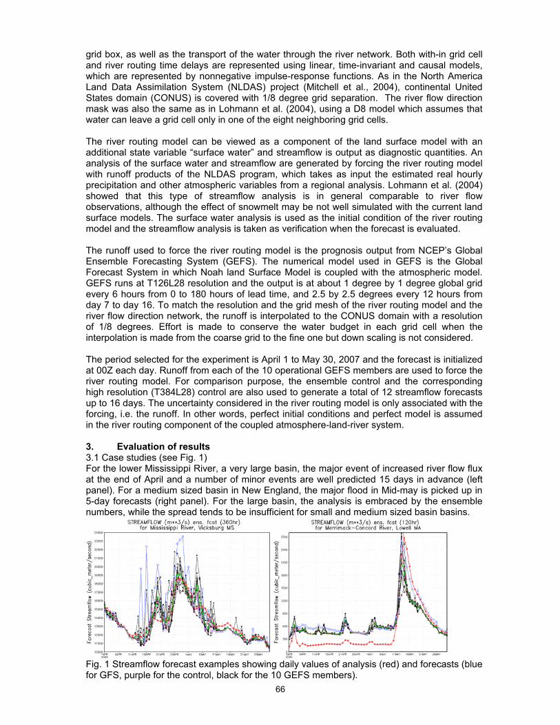
66

grid box, as well as the transport of the water through the river network. Both with-in grid cell and river routing time delays are represented using linear, time-invariant and causal models, which are represented by nonnegative impulse-response functions. As in the North America Land Data Assimilation System (NLDAS) project (Mitchell et al., 2004), continental United States domain (CONUS) is covered with 1/8 degree grid separation. The river flow direction mask was also the same as in Lohmann et al. (2004), using a D8 model which assumes that water can leave a grid cell only in one of the eight neighboring grid cells. The river routing model can be viewed as a component of the land surface model with an additional state variable “surface water” and streamflow is output as diagnostic quantities. An analysis of the surface water and streamflow are generated by forcing the river routing model with runoff products of the NLDAS program, which takes as input the estimated real hourly precipitation and other atmospheric variables from a regional analysis. Lohmann et al. (2004) showed that this type of streamflow analysis is in general comparable to river flow observations, although the effect of snowmelt may be not well simulated with the current land surface models. The surface water analysis is used as the initial condition of the river routing model and the streamflow analysis is taken as verification when the forecast is evaluated. The runoff used to force the river routing model is the prognosis output from NCEP’s Global Ensemble Forecasting System (GEFS). The numerical model used in GEFS is the Global Forecast System in which Noah land Surface Model is coupled with the atmospheric model. GEFS runs at T126L28 resolution and the output is at about 1 degree by 1 degree global grid every 6 hours from 0 to 180 hours of lead time, and 2.5 by 2.5 degrees every 12 hours from day 7 to day 16. To match the resolution and the grid mesh of the river routing model and the river flow direction network, the runoff is interpolated to the CONUS domain with a resolution of 1/8 degrees. Effort is made to conserve the water budget in each grid cell when the interpolation is made from the coarse grid to the fine one but down scaling is not considered. The period selected for the experiment is April 1 to May 30, 2007 and the forecast is initialized at 00Z each day. Runoff from each of the 10 operational GEFS members are used to force the river routing model. For comparison purpose, the ensemble control and the corresponding high resolution (T384L28) control are also used to generate a total of 12 streamflow forecasts up to 16 days. The uncertainty considered in the river routing model is only associated with the forcing, i.e. the runoff. In other words, perfect initial conditions and perfect model is assumed in the river routing component of the coupled atmosphere-land-river system. 3. Evaluation of results 3.1 Case studies (see Fig. 1) For the lower Mississippi River, a very large basin, the major event of increased river flow flux at the end of April and a number of minor events are well predicted 15 days in advance (left panel). For a medium sized basin in New England, the major flood in Mid-may is picked up in 5-day forecasts (right panel). For the large basin, the analysis is embraced by the ensemble numbers, while the spread tends to be insufficient for small and medium sized basin basins.

Fig. 1 Streamflow forecast examples showing daily values of analysis (red) and forecasts (blue for GFS, purple for the control, black for the 10 GEFS members).

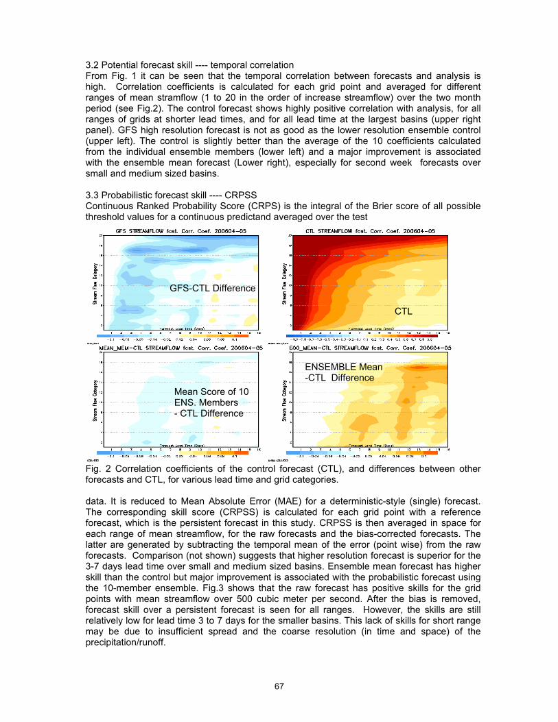
67

3.2 Potential forecast skill ---- temporal correlation From Fig. 1 it can be seen that the temporal correlation between forecasts and analysis is high. Correlation coefficients is calculated for each grid point and averaged for different ranges of mean stramflow (1 to 20 in the order of increase streamflow) over the two month period (see Fig.2). The control forecast shows highly positive correlation with analysis, for all ranges of grids at shorter lead times, and for all lead time at the largest basins (upper right panel). GFS high resolution forecast is not as good as the lower resolution ensemble control (upper left). The control is slightly better than the average of the 10 coefficients calculated from the individual ensemble members (lower left) and a major improvement is associated with the ensemble mean forecast (Lower right), especially for second week forecasts over small and medium sized basins. 3.3 Probabilistic forecast skill ---- CRPSS Continuous Ranked Probability Score (CRPS) is the integral of the Brier score of all possible threshold values for a continuous predictand averaged over the test

Fig. 2 Correlation coefficients of the control forecast (CTL), and differences between other forecasts and CTL, for various lead time and grid categories. data. It is reduced to Mean Absolute Error (MAE) for a deterministic-style (single) forecast. The corresponding skill score (CRPSS) is calculated for each grid point with a reference forecast, which is the persistent forecast in this study. CRPSS is then averaged in space for each range of mean streamflow, for the raw forecasts and the bias-corrected forecasts. The latter are generated by subtracting the temporal mean of the error (point wise) from the raw forecasts. Comparison (not shown) suggests that higher resolution forecast is superior for the 3-7 days lead time over small and medium sized basins. Ensemble mean forecast has higher skill than the control but major improvement is associated with the probabilistic forecast using the 10-member ensemble. Fig.3 shows that the raw forecast has positive skills for the grid points with mean streamflow over 500 cubic meter per second. After the bias is removed, forecast skill over a persistent forecast is seen for all ranges. However, the skills are still relatively low for lead time 3 to 7 days for the smaller basins. This lack of skills for short range may be due to insufficient spread and the coarse resolution (in time and space) of the precipitation/runoff.

CTL

ENSEMBLE Mean-CTL Difference

Mean Score of 10 ENS. Members - CTL Difference

GFS-CTL Difference

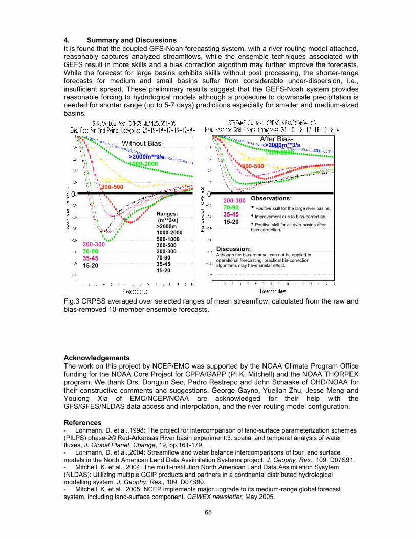
68

4. Summary and Discussions It is found that the coupled GFS-Noah forecasting system, with a river routing model attached, reasonably captures analyzed streamflows, while the ensemble techniques associated with GEFS result in more skills and a bias correction algorithm may further improve the forecasts. While the forecast for large basins exhibits skills without post processing, the shorter-range forecasts for medium and small basins suffer from considerable under-dispersion, i.e., insufficient spread. These preliminary results suggest that the GEFS-Noah system provides reasonable forcing to hydrological models although a procedure to downscale precipitation is needed for shorter range (up to 5-7 days) predictions especially for smaller and medium-sized basins.

Fig.3 CRPSS averaged over selected ranges of mean streamflow, calculated from the raw and bias-removed 10-member ensemble forecasts. Acknowledgements The work on this project by NCEP/EMC was supported by the NOAA Climate Program Office funding for the NOAA Core Project for CPPA/GAPP (PI K. Mitchell) and the NOAA THORPEX program. We thank Drs. Dongjun Seo, Pedro Restrepo and John Schaake of OHD/NOAA for their constructive comments and suggestions. George Gayno, Yuejian Zhu, Jesse Meng and Youlong Xia of EMC/NCEP/NOAA are acknowledged for their help with the GFS/GFES/NLDAS data access and interpolation, and the river routing model configuration. References - Lohmann, D. et al.,1998: The project for intercomparison of land-surface parameterization schemes (PILPS) phase-2© Red-Arkansas River basin experiment:3. spatial and temperal analysis of water fluxes, J. Global Planet. Change, 19, pp.161-179. - Lohmann, D. et al.,2004: Streamflow and water balance intercomparisons of four land surface models in the North American Land Data Assimilation Systems project. J. Geophy. Res., 109, D07S91. - Mitchell, K. et al., 2004: The multi-institution North American Land Data Assimilation Sysytem (NLDAS): Utilizing multiple GCIP products and partners in a continental distributed hydrological modelling system. J. Geophy. Res., 109, D07S90. - Mitchell, K. et al., 2005: NCEP implements major upgrade to its medium-range global forecast system, including land-surface component. GEWEX newsletter, May 2005.

Ranges: (m**3/s) >2000m 1000-2000 500-1000 300-500 200-300 70-90 35-45 15-20

>2000m**3/s 1000-2000

500-1000 300-500

200-300 70-90 35-45 15-20

>2000m**3/s 1000-2000

500-1000 300-500

200-30070-90 35-45 15-20

Without Bias- After Bias-

00

Discussion: Although the bias-removal can not be applied in operational forecasting, practical bia-correction algorithms may have similar effect.

Observations:• Positive skill for the large river basins.

• Improvement due to bias-correction.

• Positive skill for all river basins after bias correction.

69

Hydroelectric Operations - Ensemble Optimization Procedures (EOP) by C. D. D. Howard

Hydroelectric Operations - Ensemble Optimization Procedures (EOP) Charles D. D. Howard Senior Advisor, Consulting Engineer Victoria, BC, Canada cddhoward@shaw.ca ABSTRACT Weather forecasts provide the basic information used in forecasting electrical loads and hydrologic inputs to reservoirs. A conventional approach in load forecasting accounts for seasonal trends, currently observed loads, and a random component based on the statistics of past electrical loads. Conventional hydrologic forecasting takes a similar approach but with added complexity from hydrologic behavior of the contributing basin and routing in the river systems. In both cases a single deterministic weather forecast is the basic input. HEPEX may change conventional hydroelectric practice by basing the end user product, forecasts of electrical load or reservoir inflow, on sets of equally likely weather forecasts. Hydroelectric operating decisions will then require support from an Ensemble Optimization Procedure (EOP) that explicitly considers the set of forecasts (the ensemble) in recommending the best possible decisions at the current time. This paper discusses the data management and interface requirements for practical implementation and demonstrates the application of an EOP to scheduling operation of a cascade of seven hydroelectric generating stations.

70

K-L

Evaluation of the medium-range European flood forecasts for the March-April 2006 flood in the Morava river by M. Kalas, M.H. Ramos and J. Thielen EVALUATION OF THE MEDIUM-RANGE EUROPEAN FLOOD FORECASTS FOR THE MARCH-APRIL 2006 FLOOD IN THE MORAVA RIVER Milan Kalas1,, Maria-Helena Ramos2, Jutta Thielen1

1 European Commission, DG Joint Research Centre, Institute for Environment and Sustainability, TP261, 21020 2 Cemagref Lyon, Hydrology and Hydraulics Research Unit, France. E-mail: ramos@lyon.cemagref.fr Abstract The European Flood Alert System (EFAS) is a research project which aims at extending to 3-10 days the lead-time of flood forecasts in transnational river basins. The main objective is to complement Member States’ activities on flood forecasting and increase preparedness by providing earlier and additional information on potential flood situations. As a research project in a development phase, EFAS has been subject of continuous improvements aiming at a better simulation of the physical processes involved in river basin hydrology and therefore better accuracy in its forecasts. This paper presents some recent developments introduced on the calibration of the hydrological LISFLOOD model used in EFAS. We investigate the case of the March-April 2006 flood event of the Morava River. From 29th March to 09th April 2006, the Morava catchment in the Danube River basin was hit by severe flooding caused by snow melting and rainfall. The floods affected settlements and agricultural lands in Slovakia, Czech Republic and Austria. In the downstream Morava, 100-year flood and more peak discharges were observed. Forecasts based on deterministic and probabilistic weather forecasts are presented and verified against observed data.

71

Improving precipitation generation for seasonal hydrological prediction by L. Luo and E.F. Wood

Improving precipitation generation for seasonal hydrologic prediction Lifeng Luo 1,2,*, Eric F. Wood 1

1 Environmental Engineering and Water Resources, Department of Civil and Environmental Engineering, Princeton University, Princeton, NJ 08544, USA 2 Program in Atmospheric and Oceanic Sciences, Princeton University, Princeton, NJ 08543, USA * Corresponding author: Lifeng Luo, Dept. Civil and Environmental Engineering, Princeton University, Princeton, NJ 08544, USA. +1 (609) 258-1551, lluo@princeton.edu Abstract One major challenge in seasonal hydrologic prediction is the proper representation of the uncertainties in the atmospheric forcing during the forecast period. These uncertainties are not only naturally associated with the predictability of the climate system at seasonal timescales, but are also affected by the method that is used to produce the atmospheric forcing time series at daily or sub-daily timescales. Various studies have explored different methods to generate atmospheric forcing time series, such as the K-nearest neighbor resampling scheme and the Schaake shuffle method. Most of these methods are based on use of historical observations. In particular, Luo and Wood (2007) uses selected observed historical meteorology as the forcing basis and then adjust them to match the predicted monthly mean values. These monthly mean values are derived from seasonal climate predictions from dynamic climate models. This study attempts to improve the forcing generation method in Luo and Wood (2007) by addressing the following two questions: 1) How can we fully use information provided by seasonal climate predictions from dynamic climate models in creating atmospheric forcing sequences? 2) At various spatial and temporal scales, what are the required levels of skill in seasonal climate prediction to make it useful for hydrologic predictions? As presented by Luo and Wood (2006), variations at larger spatial scales and longer time scales are potentially more predictable by climate models. For instance, the forecast of 6-month total precipitation is likely to be more skillful than the forecast of the total precipitation of the 6th month. In this study, adjustments to selected historical records are performed at different temporal scales according to the corresponding skill level of the seasonal climate predictions. By selecting the time period, accuracy and number of adjustments to the historical forcing records, we can quantify the usefulness of climate predictions across space and time. References

- Luo, L and E. F. Wood, Seasonal hydrologic prediction with the VIC hydrologic model for the Ohio River basin, submitted to J. Hydromet.

- Luo, L., and E. F. Wood (2006), Assessing the idealized predictability of precipitation and temperature in the NCEP Climate Forecast System, Geophys. Res. Lett., 33, L04708, doi:10.1029/2005GL025292.

72

M-N

Matching time-steps and updating cycle of meteorological PQPF’s to fit hydrological needs and to produce ensemble discharge forecasts by R. Marty, A. Djerboua, I. Zin and Ch. Obled

MATCHING TIME-STEPS AND UPDATING CYCLE OF METEOROLOGICAL PQPF’s TO FIT HYDROLOGICAL NEEDS AND TO PRODUCE ENSEMBLE DISCHARGE FORECASTS. Marty R.1, Djerboua A.2, Zin I.1* and Obled Ch. 1

1 INPG/LTHE, Grenoble, France 2 RHEA, Nanterre, France * Corresponding Author: Isabella Zin, BP 53 38041 Grenoble Cedex 9 France, 33 (0) 4 76 82 50 52, isabella.zin@hmg.inpg.fr A simple but rather complete hydro-meteorological forecasting chain will be described, aiming at ensemble flash flood forecasts for medium-sized catchments. It can be organised into four modules : first, a system collecting hydro-meteorological observations and their related database; second, a module gathering meteorological forecasts from different suppliers and processing these data in order to satisfy the hydrological model requirements; third, a hydrological model using observations and forecasts as inputs to provide forecasts of river heights and/or discharges; finally, an hydraulic component manages flow propagation and flooding, and could be coupled with a GIS containing information about the vulnerability of the predicted flooded areas to help the decision-maker. In this paper special focus will be put on module two, i.e. on the use of different precipitation forecasts within the chain. These precipitation forecasts can be either deterministic or probabilistic. They may consist of both immediate (lead-time up to 2 hours) and/or short-term forecasts (lead-time up to 36 or 48 hours). However, they are generally not specific to the considered catchment and are often provided at a meteorological time-step (usually, 12 or 24 hours) which is not appropriate for quick responding catchments (hydrological time-step needed of 1 hour or even less). Here, we shall focus on the use of probabilistic quantitative precipitation forecasts (PQPFs) such as those proposed by an Analog technique - cf. Obled et al. in this workshop. They are expressed as the distribution of catchment averaged precipitation totalised over rather large time-step (e.g. daily), compared to what is required for hydrological modelling. Thus, for flash floods forecasting, it is necessary to disaggregate these forecasts down to the hydrological model time-step (here, 1 hour), while preserving the prescribed forecasts distribution. The presentation proposes such a way to match current meteorological and hydrological lead-times through the use of a simple rainfall generator capable of running in real time. Another set of operational constraints come from the need to take into account the updating cycle of the meteorological forecasts (every day at 6h UTC in the case presented). The use of other qualitative available information (e.g. precipitation ending time) will also be addressed. The post-processed precipitation forecasts are then given in terms of predicted hourly rainfall scenarios which are used as inputs to the hydrological model and converted into predicted discharge scenarios in order to give ensemble flood forecasts. These are also given in term of probability of exceeding a given discharge threshold. This will be illustrated on a case study concerning flash flood forecasts in the Cevennes region (Southern France).

73

Probabilistic Streamflow forecast in norway by M. Morawietz, T. Skaugen and E. Langsholt Probabilistic streamflow forecast in Norway Martin Morawietz1, Thomas Skaugen1,2 and Elin Langsholt2

1 Department of Geosciences, University of Oslo, Norway 2 Norwegian Water Resources and Energy Directorate, Oslo, Norway Corresponding author: Martin Morawietz, Department of Geosciences, University of Oslo, P.O. Box 1047 Blindern, 0316 Oslo, Norway, ++47 22856695, martin.morawietz@geo.uio.no Abstract A forecast procedure for short to medium range (1-6 days) probabilistic streamflow forecast, developed and implemented for Norwegian catchments, is presented. The procedure consists of: (1) the deterministic meteorological forecast of temperature and precipitation, (2) a stochastic pre-processor that accounts for the uncertainty of the meteorological forecast, (3) a hydrological model (HBV model) that transforms precipitation and temperature input to streamflow output, and (4) a stochastic post-processor that accounts for the uncertainty of the hydrological model. In a Monte Carlo simulation, an ensemble of streamflow values is generated that is interpreted as probabilistic streamflow forecast. For future work, this procedure forms the basis for comparison with other methods of ensemble streamflow prediction. The procedure will be compared to procedures that are based on meteorological ensemble forecasts as input. Further, pre- and post-processor of the system will be compared with components of the ensemble streamflow prediction system developed at NOAA. 1. Introduction Based on the experiences from a major flood in Eastern Norway in 1995, a project was initiated and administered by the Norwegian Water Resources and Energy Directorate (NVE) with the aim to quantify the uncertainty associated with the streamflow forecasts issued by NVE (Skaugen et. al, 2006). The Norwegian Computing Center developed stochastic model components that describe the error of the meteorological forecast (Follestad and Høst, 1998) and the error of the hydrological model (Langsrud et al., 1998). By combining the error models in a Monte Carlo simulation together with the hydrological model (Langsrud et al., 1999), an ensemble of streamflow values is generated which can be interpreted as a probabilistic streamflow forecast. The procedure was tested and implemented at NVE (Skaugen et. al, 2006). It is calibrated in 79 catchments, where streamflow forecasts with a lead time of up to six days are issued. In the following sections, the components of the probabilistic streamflow forecast procedure are presented. They form the basis for further work which is outlined in the last section. 2. Pre-processor: Uncertainty in precipitation and temperature forecast To describe the uncertainty of the temperature and precipitation forecast, Follestad and Høst (1998) developed stochastic models for the distribution of the observed temperature and precipitation conditioned on the forecasted values. Temperature The model for temperature,

⎪⎩

⎪⎨

⎧

<+−++

>=+−++=

−−

−−

0)(

0)(

)()()(11

)(5

)()(3

)(1

)()()(11

)(4

)()(2

)(0

jt

jneg

jtt

jjt

jj

jt

jpos

jtt

jjt

jj

t

SforSTS

SforSTST

εααα

εααα (1)

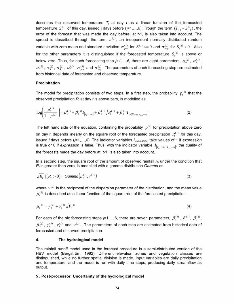
74

describes the observed temperature Tt at day t as a linear function of the forecasted temperature )( j

tS of this day, issued j days before (j=1,…,6). Trough the term )( )(11j

tt ST −− − , the error of the forecast that was made the day before, at t-1, is also taken into account. The spread is described through the term )( jε , an independent normally distributed random

variable with zero mean and standard deviation )( jposσ for 0)( >=j

tS and )( jnegσ for 0)( <j

tS . Also

for the other parameters it is distinguished if the forecasted temperature )( jtS is above or

below zero. Thus, for each forecasting step j=1,…,6, there are eight parameters, )(0

jα , )(1

jα , )(

2jα , )(

3jα , )(

4jα , )(

5jα , )( j

posσ and )( jnegσ . The parameters of each forecasting step are estimated

from historical data of forecasted and observed temperature. Precipitation The model for precipitation consists of two steps. In a first step, the probability )( j

tp that the observed precipitation Rt at day t is above zero, is modelled as

[ ] [ ]00)(

3)()(

20)(

1)(

0)(

)(

1)(

1)(

1log

==>> −−+++=⎟⎟

⎠

⎞⎜⎜⎝

⎛− t

jt

jt RP

jjt

jP

jjj

t

jt IPIp

pΙ

ββββ (2)

The left hand side of the equation, containing the probability )( j

tp for precipitation above zero

on day t, depends linearly on the square root of the forecasted precipitation )( jtP for this day,

issued j days before (j=1,…,6). The indicator variables I[expression] take values of 1 if expression is true or 0 if expression is false. Thus, with the indicator variable [ ]00 1

)(1 ==> −− tj

t RPI

Ι, the quality of

the forecasts made the day before at, t-1, is also taken into account. In a second step, the square root of the amount of observed rainfall Rt under the condition that Rt is greater than zero, is modelled with a gamma distribution Gamma as

( ) ( ))()( ,0| jjttt GammaRR νμ=> (3)

where )( jν is the reciprocal of the dispersion parameter of the distribution, and the mean value

)( jtμ is described as a linear function of the square root of the forecasted precipitation:

)()(

1)(

0)( j

tjjj

t Pγγμ += (4) For each of the six forecasting steps j=1,…,6, there are seven parameters, )(

0jβ , )(

1jβ , )(

2jβ ,

)(3

jβ , )(0

jγ , )(1

jγ and )( jν . The parameters of each step are estimated from historical data of forecasted and observed precipitation. 4. The hydrological model The rainfall runoff model used in the forecast procedure is a semi-distributed version of the HBV model (Bergström, 1992). Different elevation zones and vegetation classes are distinguished, while no further spatial division is made. Input variables are daily precipitation and temperature, and the model is run with daily time steps, producing daily streamflow as output. 5 . Post-processor: Uncertainty of the hydrological model

75

A stochastic model for the error of the hydrological model, the HBV model, was developed by Langsrud et al. (1998). The error is modelled as a first order autoregressive process, i.e. the error dt on day t depends on the error dt_1 of the day before, as:

ttttt udd σα += −1 (5) where the error dt is the difference between the log-transformed values of observed streamflow )(tQobs and simulated streamflow )(tQsim at day t:

)(ln)(ln tQtQd simobst −= (6) In equation (5), ut is an independent standard normally distributed random variable, and αt and σt are described as functions of the log-transformed simulated streamflow according to:

)(ln)( tQba simtit +=α (7)

)(lnln )( tQBA simtit +=σ (8) The parameters )(tia and )(tiA have different values for different combinations of: a.) observed temperature Tt : above or below zero, and in case of temperature above zero: b.) observed precipitation Rt : zero or larger than zero, c.) snow reservoir in the HBV model: present or not. In addition, the parameters )(tia , )(tiA , b and B have different values depending on: d.) simulated streamflow Qsim(t): above or below a certain threshold (the 75% non- exceedance percentile is chosen as threshold in the current implementation of the procedure). Accounting for the different combinations, the total number of parameters )(tia , )(tiA , b and B for the error model of the HBV model is 24. The parameters are estimated from historical data of observed and simulated streamflow, where the simulated streamflow is modelled with observed precipitation and temperature. 5. Total uncertainty of the streamflow forecast The total uncertainty of the streamflow forecast is determined in a Monte Carlo simulation. Using equations (1), (2) and (3), possible realizations of the future temperature *

tT and

precipitation *tP are generated based on the deterministic forecast of temperature )( j

tS and

precipitation )( jtP . The pairs of possible temperature *

tT and precipitation *tP (in the current

implementation 1000) are then treated as if they where true values of temperature tT and

precipitation tP . Possible future streamflow values are generated from the ( *tT , tP ) pairs using

the HBV model. After adding a hydrological error from equation (5) to each of the HBV-outputs, the resulting set of streamflow values is interpreted as a probabilistic streamflow forecast. 6. Outlook The probabilistic forecast procedure outlined above (NVE procedure) forms the basis for future work.

76

The procedure will be compared to procedures that use meteorological ensemble forecasts instead of the deterministic meteorological forecast as starting point for the description of the uncertainty of the streamflow forecast. The 51 member ensemble forecasts of the European Center for Medium Range Weather Forecast will be used as well as short range limited area ensemble forecasts with 21 members from the Norwegian weather service Met.no (Jensen et al., 2005). Procedures of different complexities will be set up and compared to the NVE procedure. Furthermore, the pre- and post-processor of the NVE procedure will be compared to components of the streamflow ensemble prediction system developed at NOAA. This comprises the pre-processor developed by Schaake et al. (2007) and the post-processor developed by Seo et al (2006). It is planned to apply the procedures to both Norwegian and US catchments, using meteorological forecast data from ECMWF/Met.no and NCEP respectively. References

- Bergström, S., 1992. The HBV model – its structure and applications. SMHI Reports Hydrology no 4, Swedish Meteorological and Hydrological Institute, Norrköping, Sweden.

- Follestad, T., Høst, G. 1998. A statistical model for the uncertainty in meteorological forecasts with application to the Knappom and Røykenes catchments. HYDRA note no 12, Oslo, Norway (available from NVE).

- Jensen, M. H., Frogner, I.-L., Iversen, T., Vignes, O. 2005. Limited area ensemble forecasting in Norway using targeted EPS. ECMWF Newsletter 107, 23-29.

- Langsrud, Ø., Frigessi, A., Høst, G. 1998. Pure modell error of the HBV modell. HYDRA note no 4, Oslo, Norway (available from NVE).

- Langsrud, Ø, Høst, G., Follestad, T., Frigessi, A. 1999. Quantifying uncertainty in HBV runoff forecasts by stochastic simulations. HYDRA note no 2, Oslo, Norway (available from NVE).

- Lundquist, D. 1997. Flood forecasting in practice. Paper presented at the European Geophysical Society, XXII General Assembly, Vienna, Austria, 21-25 April 2007.

- Schaake, J., Demargne, J., Hartman, R.,. Mullusky, M., Welles, E., Wu, L., Herr, H., Fan, X., Seo, D.J. 2007. Precipitation and temperature ensemble forecasts from single-value forecasts. Hydrol. Earth Syst. Sci. Discuss. 4(2), 655-717.

- Seo, D.-J., Herr, H.D., Schaake, J.C. 2006. A statistical post-processor for accounting of hydrologic uncertainty in short-range ensemble streamflow prediction. Hydrol. Earth Syst. Sci. Discuss. 3(4), 1987-2035.

- Skaugen, T., Langsholt, E., Langsrud, Ø., Follestad, T., Høst, G. 2006. Uncertainty in flood forecasting. In: Refsgaard, J.C., Højberg, A.L. eds. Nordic Water 2006. Proceedings of the XXIV Nordic Hydrological Conference. NHP report no 49. 674-680.

77

Hydrological climate change impact assessment over the Blue Nile using ensemble statistical downscaling by R. Nawaz, T. Belleby and M. Elshamy

HYDROLOGICAL CLIMATE CHANGE IMPACT ASSESSMENT OVER THE BLUE NILE USING ENSEMBLE STATISTICAL DOWNSCALING Rizwan Nawaz 1*, Tim Belleby2 and Mohammed Elshamy3 1 Earth and Biosphere Institute, University of Leeds, UK. 2 University of Hull, UK 3 Nile Forecast Center, Ministry of Water Resources and Irrigation, Egypt. * Corresponding author: N.R.Nawaz, Earth and Biosphere Institute, University of Leeds, Leeds, LS2 9JT, UK. 0113 3433362 n.r.nawaz@leeds.ac.uk Abstract The sensitivity of Blue Nile flows to changes in future rainfall during the June–September rainy season was studied using output from three General Circulation Models (GCMs). The study attempted to quantify uncertainties arising from: (a) use of different GCMs; (b) different greenhouse gas emissions scenarios; and (c) downscaling coarse-scale GCM output to a finer-scale required for hydrological modelling. A multidimensional stochastic rainfall generator was developed to produce high-resolution gridded rainfall data required by an established operational distributed hydrological model. 1. Introduction The aim of this study was to undertake an investigation of the sensitivity of Blue Nile flow to climate change and to assess the extent of precipitation-related uncertainty in this context. A major goal of the study was to use off-the-shelf GCM data to drive a relatively high resolution operational gridded hydrological model (20 × 20 km and daily time-step). The study employed three GCMs, forced with two sets of greenhouse gas emissions scenarios; the output from which was downscaled using an ensemble approach employing a multidimensional stochastic rainfall generator. Downscaled precipitation scenarios were used to drive the NFS hydrological model (Nile Forecasting System: Schaake et al., 1996; Elshamy, 2006) to assess the impacts of climate change on both mean flow as well as the flow exceeding 5% and 1% of the time during the wet season (June–September). the main rainy season in the region. 2. Methodology The study was carried out in four steps: (i) Gather Blue Nile Basin historical daily rainfall data and GCM monthly rainfall data over a baseline period; (ii) elect several GCMs on the basis of their performance in simulating current climate; (iii) calibrate a stochastic rainfall generator; and (iv) use rainfall generator to generate 50 traces of baseline and future rainfall and feed both baseline and future rainfall data into the NFS to determine future Blue Nile flow changes. 2.1 GCM selection GCM selection was based on model ability to simulate historical baseline rainfall and a number of GCMs were tested for their adequacy. The mean monthly GCM-simulated rainfall over 1992–2001 simulated by three different GCMs: (i) CGCM2 (The Canadian Climate Modelling Centre); (ii) ECHAM4 (Max Planck Institute for Meteorology, Hamburg); and (iii) HADCM3 (UK Hadley Centre) compared well with observational data over the same period. Two sets of greenhouse gas (GHG) emissions scenarios were used; the SRES A2 and B2, which make different assumptions about future global socio-economic conditions (see IPCC, 2000). 2.2 Downscaling The implementation of a statistical downscaling approach requires the establishment of quantitative relationships between GCM-derived predictor variables and local rainfall statistics. However, standard GCM runs reproduce climate variability, rather than simulating observed weather patterns and it is not possible to match GCM timelines directly to observed data. Observed data may be used as a proxy for specific GCM outputs but this approach does not

78

directly address the uncertainty in the GCM outputs. GCM runs forced to observed Sea Surface Temperature (SST) data may also be used but these are less readily available. This study employed a third alternative, employing histogram matching (Rosenfeld et al., 1993) to compare the frequency distributions of standard GCM outputs and local rainfall statistics. If a predictor, T, with cumulative distribution F(T) and predictand S, with cumulative distribution G(S), are monotonically related by S=f(T), then f(T)=G-1(F(T)). It is thus possible to derive f(T) from F(T) and G(S) without needing to match individual pairs of data points. Moreover, the distribution of estimates of S should closely match those for the observed data, even if the relationship between T and S is relatively weak. While the local distributions of both GCM outputs and daily rainfall statistics will vary with both geographical location and season, it is advantageous to assume an invariant relationship between predictor and predictand to accommodate spatial movement of climatological patterns over time. Separate distributions, F(T) and G(S), were derived for each calendar month and grid box within the baseline dataset and a standard non-linear regression technique used to derive a single relationship, S=f(T), that applied across all months and locations. Statistical relationships were derived between GCM outputs and three statistics (i) probability of a wet day given a previously wet day (PWW); (ii) probability of a wet day given a previously dry day (PWD) and (iii) daily rainfall amount on a wet day (MRR). The daily statistics were obtained from synoptic station data block-krigged to the NFS model resolution of 20km for cells containing a recording gauge. Months where missing values exceeded a 10-day threshold were discarded. Separate relationships were derived for each selected GCM. In all cases, the regression equations were able to explain a significant amount of variation with R2 values exceeding 0.70. 2.3 Multidimensional stochastic rainfall generator Daily 20km spatial resolution rainfall data were generated using up a stochastic rainfall generator based on the Turning Bands method (Mantoglou, 1987). The spatial structure of the rainfall field was modelled using a homogeneous, isotropic exponential model for spatial covariance while temporal correlation was addressed using the parameters; PWW, PWD derived above. The rainfall distribution on a rainy day was modelling using a two-parameter gamma distribution scaled by MRR. The orographic rainfall component associated with the Ethiopian Highlands was modelled using a spatially-varying multiplicative factor derived by comparing the long-term averages of observed and uncorrected simulated rainfall over the baseline period. 2.4 Potential evapotranspiration Monthly mean baseline and future temperature simulated by all three GCMs were used with the Thornthwaite formula (Thornthwaite, 1948) to determine current and future monthly mean PET and the corresponding percentage changes which were applied to the observational PET dataset. 2.5 Hydrological modelling The NFS is an operational distributed hydro-meteorological forecasting system designed for forecasting Nile flows at designated key points within the Nile Basin. The core of the NFS is a conceptual distributed hydrological model (Johnson & Curtis, 1994; Schaake et al., 1996) including soil moisture accounting, hillslope and river routing, lakes, wetlands, and man-made reservoirs within the basin. The NFS requires as input, daily gridded rainfall and potential evapotranspiration. Three basic models are normally executed at every grid cell: (i) water balance model; (ii) hillslope model; and (iii) channel routing model (Nile Forecast Center, 1999). While the NFS includes an optional data assimilation procedure, it is specifically designed to be capable of both forecasting and simulation of the Nile Basin and is able to reproduce the flow regime over long periods accurately without state updating. Further details of the NFS and its evaluation in long term simulations are provided in Elshamy (2006).

79

3. Results Figure 1 shows the future change (percentage from baseline) in flow at Diem station for the wet season (June–September). Changes are presented as box-plots showing the range of downscaling-related uncertainty (10%, 25%, 50%, 75% and 90% ensemble quantiles). By considering only the inter-quartile range in the box plots, it can be concluded that significant changes are to be expected in flow during all three time- periods. The CGCM indicates drier conditions driven by the rainfall scenarios. The marked difference between projected flow reductions under the CGCM A2 and B2 scenarios for the 2050s is noteworthy. Results from HadCM3 suggest that although a wetter future is expected, flow is set to decrease, especially by the 2080s. This is because increased PET across the basin leads to flow reduction even though rainfall increases by a small amount. The ensemble medians indicate that the percentage change in mean flow could vary from –46.6% (CGCM A2 2080s) to +12.4% (ECHAM B2 2050s). Q5 shows similar reductions but a greater increase (32.1% increase under the ECHAM B2 2050s). However, the ensemble inter-quartile ranges reveal the effects of downscaling uncertainty, leading to a greater variation in the percentage change in mean flow: from –48.5% (CGCM2 A2 2080s) to +17.9% (ECHAM B2 2050s). This large variation corresponds to limits within the 75th and 25th percentiles and would be even greater had results been presented in between the 90th and 10th percentiles. Conclusions This study assessed Blue Nile flow response to uncertainties in: (i) future GHG emissions; (ii) GCMs; and (iii) downscaling GCM output to a finer spatio-temporal scale. The findings indicate that considerable variations in Blue Nile flow sensitivity arise as a result of GHG emissions uncertainties and choice of GCM. In the Blue Nile case study area, one GCM indicates a drier future, whilst two others indicate wetter futures. Uncertainties introduced by the downscaling procedure (which include some element of GCM rainfall uncertainty) were also quantified and shown to be significant. Under the majority of the scenarios, it was shown that future Blue Nile flow is generally expected to reduce, despite small increases in future rainfall; this is because of large projected increases in PET which offsets small increases in rainfall. This warrants a more detailed examination of the effect of future PET changes on Blue Nile flow. A further limitation of the study is that it did not consider additional sources of uncertainty including sampling and hydrological model uncertainties, which can also be significant. The results presented in this study are in general agreement with what other investigators have noted. Riebsame et al. (1995) reported that GCM scenarios provided widely diverging pictures of possible future river flows, from a 30% increase to a 78% decrease; larger reductions were expected as is the case in the present study. Yates and Strzepek (1998) reported a range of changes for a doubling of CO2 concentrations; mean annual flow was expected to change by –19% (CGCM1), +41% (ECHAM1) and +133% (HadCM1). Although the sign of changes is consistent with findings from the present study, the flow sensitivity appears to be much greater, especially under the HadCM1 scenario due to a large projected increase in rainfall.

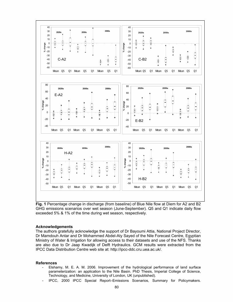
80

Fig. 1 Percentage change in discharge (from baseline) of Blue Nile flow at Diem for A2 and B2 GHG emissions scenarios over wet season (June-September). Q5 and Q1 indicate daily flow exceeded 5% & 1% of the time during wet season, respectively. Acknowledgements The authors gratefully acknowledge the support of Dr Bayoumi Attia, National Project Director, Dr Mamdouh Antar and Dr Mohammed Abdel-Aty Sayed of the Nile Forecast Centre, Egyptian Ministry of Water & Irrigation for allowing access to their datasets and use of the NFS. Thanks are also due to Dr Jaap Kwadijk of Delft Hydraulics. GCM results were extracted from the IPCC Data Distribution Centre web site at: http://ipcc-ddc.cru.uea.ac.uk/. References

- Elshamy, M. E. A. M. 2006. Improvement of the hydrological performance of land surface parameterization: an application to the Nile Basin. PhD Thesis, Imperial College of Science, Technology, and Medicine, University of London, UK (unpublished).

- IPCC, 2000 IPCC Special Report–Emissions Scenarios, Summary for Policymakers.

H-B2

-60

-50

-40-30

-20

-10

0

1020

30

40

Mean Q95 Q99 Mean Q95 Q99 Mean Q95 Q99

% c

hang

e

2020s 2050s 2080s

Mean Q5 Q1 Mean Q5 Q1 Mean Q5 Q1 -60

-50

-40

-30

-20

-10

0

10

20

30

40

Mean Q95 Q99 Mean Q95 Q99 Mean Q95 Q99

% c

hang

e

2020s 2050s 2080s

Mean Q5 Q1 Mean Q5 Q1 Mean Q5 Q1

-40

-20

0

20

40

60

80

Mean Q95 Q99 Mean Q95 Q99 Mean Q95 Q99

% c

hang

e

2020s 2050s 2080s

Mean Q5 Q1 Mean Q5 Q1 Mean Q5 Q1 -40

-20

0

20

40

60

80

Mean Q95 Q99 Mean Q95 Q99 Mean Q95 Q99

% c

hang

e

2020s 2050s 2080s

Mean Q5 Q1 Mean Q5 Q1 Mean Q5 Q1

-50

-40

-30

-20

-10

0

10

20

30

40

Mean Q95 Q99 Mean Q95 Q99 Mean Q95 Q99

% c

hang

e

2020s 2050s 2080s

Mean Q5 Q1 Mean Q5 Q1 Mean Q5 Q1 -50

-40

-30

-20

-10

0

10

20

30

40

Mean Q95 Q99 Mean Q95 Q99 Mean Q95 Q99

% c

hang

e

2020s 2050s2080s

Mean Q5 Q1 Mean Q5 Q1 Mean Q5 Q1

C-A2 C-B2

E-A2

E-B2

H-A2

H-B2

81

Intergovernmental Panel on Climate Change (http://sres.ciesin.org/index.html). - Johnson, P. A. and Curtis, P. D., 1994. Water balance of Blue Nile River Basin in Ethiopia. J.

Irrig. Drain. Engng. 120, 573–589. - Mantoglou A. 1987 Digital simulation of multivariate two- and three- dimensional stochastic

processes with a spectral Turning Bands Method. Math. Geol. 19(2), 129–149. - Riebsame, W. E., Strzepek, K. M., Wescoat, J. L. Jr., Perrit, R., Graile, G. L., Jacobs, J.,

Leichenko, R., Magadza, C., Phien, H., Urbiztondo, B. J., Restrepo, P., Rose, W. R., Saleh, M., Ti, L. H., Tucci, C. & Yates, D., 1995. Complex river basins. In: Climate Changes, International Impacts and Implications (ed. by K. M. Strzepek & J. B. Smith), 57–91. Cambridge University Press, Cambridge, UK.

- Rosenfeld, D., Wolff, D. B. & Atlas, D., 1993. General probability-matched relations between radar reflectivity and rain rate. J. Appl. Met. 32(1, 50–72.

- Schaake, J. C., Koren, V. I., Duan, Q. Y., Mitchell, K. & Chen, F., 1996. Simple water balance model for estimating runoff at different spatial and temporal scales. J. Geophys. Res.-Atmos. 101(D3), 7461–7475.

- Thornthwaite, C. W., 1948. An approach toward a rational classification of climate. Geogr. Rev. 38, 55–94.

- Yates, D. & Strzepek, K. ,1998. Modelling the Nile Basin under climatic change. J. Hydrol. Engng 3(2), 98–108.

82

The groundwater recharge and meteorological data by O. Nitcheva

The groundwater recharge and meteorological data Olga Nitcheva, Institute of Water Problems at the Bulgarian Academy of Sciences Email: olganitcheva@yahoo.com Abstract The groundwater recharge could be evaluated and predicted accurately by meteorological data. The Richard’s equation for water flow from soil surface through the root zone to groundwater depends from the evapotranspiration. It is the most sensitive parameter for water dynamic in unsaturated zone. The investigations are carried out on the test field Chelopechene near to Sofia, it shows that evapotranspiration calculated by meteorological data (FAO Penman-Monteit) has the real value. The correct definition of the parameters of hydrological cycle is crucial. The growing population, the pollution of surface waters and the hazard situations force us to manage our groundwater resources. It is the only source for water supply in emergency situations.

83

O-P

Analog based post-processing of meteorological forecasts for basinwide PQPF’s: principles and operational aspects by C. Obled, A. Djerboua, R. Marty and I. Zin

ANALOG BASED POST-PROCESSING OF METEOROLOGICAL FORECASTS FOR BASINWIDE PQPF’S: PRINCIPLES AND OPERATIONAL ASPECTS Obled Ch. 1Djerboua A.2, , Marty R.1, and Zin I.1*

1 INPG/LTHE, Grenoble, France 2 RHEA, Nanterre, France * Corresponding Author: Charles Obled, BP 53 38041 Grenoble Cedex 9 France, 33 (0) 4 76 82 50 53, charles.obled@hmg.inpg.fr

Anticipating floods over quick responding catchments such as the Mediterranean ones requires an appropriate anticipation of future rainfalls.To answer this demand, we propose a probabilistic adaptation of meteorological model outputs based on an analog search for past situations similar to the expected one. The precipitation collected during those past situations allow to derive a conditional distribution for the expected rainfall which builds up the PQPF.

The calibration of such an algorithm requires several important choices such as the selection of the candidate synoptic variables to be used to describe the general circulation, the geographic window over which those variable must be considered, the criteria to be used to optimize these selections, the number of steps in the selection of the best analogs and their optimal numbers, according to the available archives, etc…

After calibration in “perfect-prog” conditions, using the 50 year NCEP/NCAR reanalyses, the current algorithm considers successively two types of analogy : the first one relies only on the general synoptic circulation, and select ~ 70 analogs while the second involves both the general synoptic circulation together with more local variables from the humidity fields. This brings down to 30 final analogs.

However, these results were obtained in perfect-prog conditions, which are not the actual conditions in real time. Depending on the model used to forecast the target situation, and on the lead-time required (e.g. 3 day ahead), the uncertainty may be growing and it has appeared necessary to relax a little the specificity of the analog selection to allow for this uncertainty. The number of analog has been optimized using the ECMWF forecast archive on 1997-2003. So it is now modulated according to the target lead-time, i.e. 30 , 40 , 50 , 70 , 130 , 500 analogs for day 1 (0-24h) to day 6 (120-144h) respectively. In some way, if the model is poor, the selection should select almost the whole archive as “analogs”, and therefore deliver the climatological average as the forecast.

Operational prototypes of this analog approach adaptation have been implemented, using the daily outputs of the American model GFS for up to 7 days lead-time. Some illustrations will be taken from the operational runs on some Mediterranean French catchment ( e.g. the catastrophic rain event of September 8 and 9th 2002 in the Gard region , but also the more recent one of 7 to 9th September 2005 showing that some early warning may be issued a few days in advance).

The daily rainfall distributions derived for each coming day and for every specific catchment are used as input to a hydrometeorological forecasting chain to derive ensemble discharge forecast (see Marty et al. this workshop). Current developments involve working on 6h-PQPF’s for the first two days ahead (0-48h), but the cornerstone is the availability of long precipitation archives with such 6h time-steps.

84

A User Guide to the Risk and uncertainty decision tree by F. Pappenberger, K. Beven, H. Harvey, D. Leedal, and J. Hall

A User Guide to the Risk and Uncertainty Decision Tree Wiki Site (www.floodrisk.net) Florian Pappenberger1,3 Keith Beven1, Hamish Harvey2, David Leedal1 and Jim Hall2

1 Lancaster Environmental Centre, Lancaster University, Lancaster LA1 4UK 2 School of Civil Engineering and Geosciences, Newcastle University, Newcastle NE1 7RU 3 now at the European Centre for Medium-Range Weather Forecasts, Reading, RG2 9AX Introduction Cascading uncertainties is an important topic within Hydrological Ensemble Prediction Systems. Considerable work has been done to catalogue the range of uncertainty methods, assess and test their applicability and demonstrate their use, with a view to promoting more widespread and rigorous use by the practitioner community. The research has been documented as an internet based Wiki site, that can be found at: http://www.floodrisk.net or http://www.floodrisknet.org.uk/methods/Introduction. The site includes • background on a variety of different risk and uncertainty assessment methods; • a decision tree to help users in choosing methods; • a glossary of terms; • a collection of Case Studies to demonstrate the use of different methods. This paper is intended to provide an overview of the Wiki site and information on how to use it. A Wiki site may be modified by the users, which means that any user can add comments or modify the text on the pages of the site, and also add case studies to augment the information on the site. The information added is recorded and then moderated by the hosts of the site (in this case, the Universities of Newcastle and Lancaster).

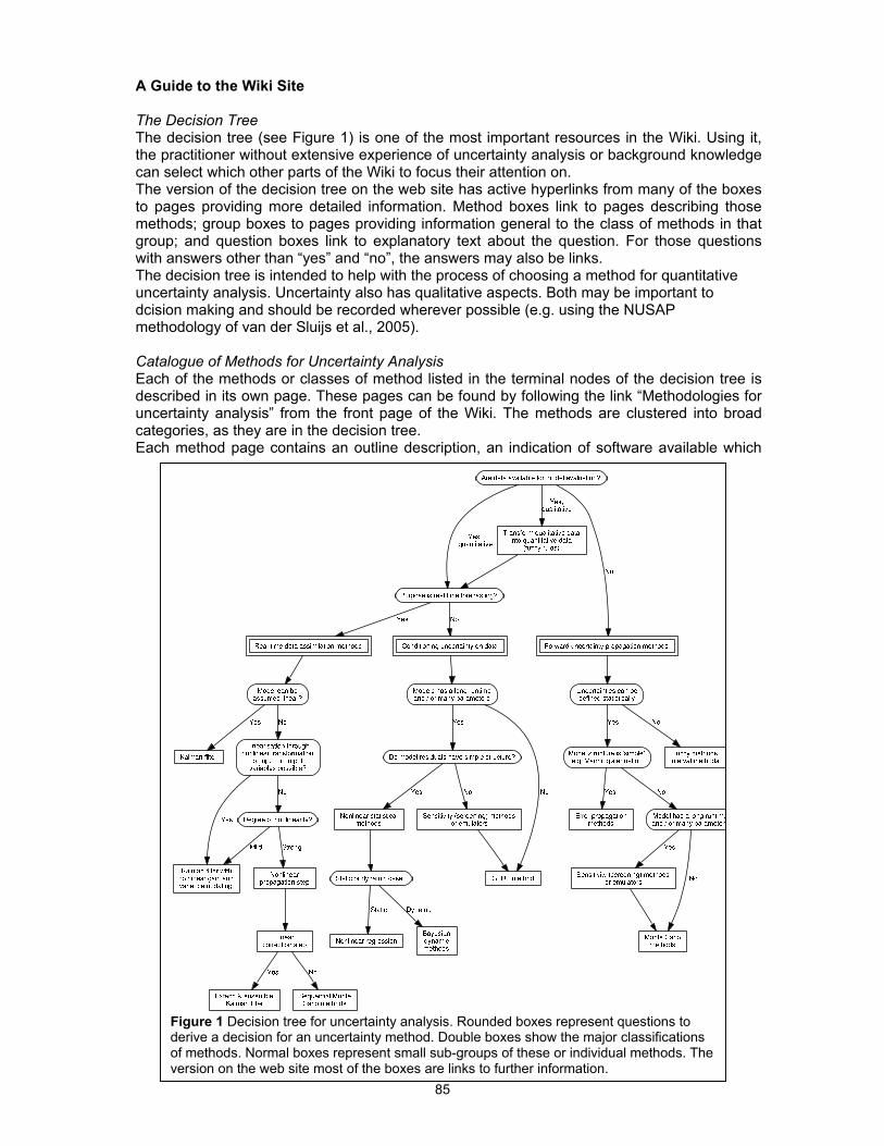
85

A Guide to the Wiki Site The Decision Tree The decision tree (see Figure 1) is one of the most important resources in the Wiki. Using it, the practitioner without extensive experience of uncertainty analysis or background knowledge can select which other parts of the Wiki to focus their attention on. The version of the decision tree on the web site has active hyperlinks from many of the boxes to pages providing more detailed information. Method boxes link to pages describing those methods; group boxes to pages providing information general to the class of methods in that group; and question boxes link to explanatory text about the question. For those questions with answers other than “yes” and “no”, the answers may also be links. The decision tree is intended to help with the process of choosing a method for quantitative uncertainty analysis. Uncertainty also has qualitative aspects. Both may be important to dcision making and should be recorded wherever possible (e.g. using the NUSAP methodology of van der Sluijs et al., 2005). Catalogue of Methods for Uncertainty Analysis Each of the methods or classes of method listed in the terminal nodes of the decision tree is described in its own page. These pages can be found by following the link “Methodologies for uncertainty analysis” from the front page of the Wiki. The methods are clustered into broad categories, as they are in the decision tree. Each method page contains an outline description, an indication of software available which

Figure 1 Decision tree for uncertainty analysis. Rounded boxes represent questions to derive a decision for an uncertainty method. Double boxes show the major classifications of methods. Normal boxes represent small sub-groups of these or individual methods. The version on the web site most of the boxes are links to further information.

86

implements the method, a list of notable advantages and disadvantages, a list of case studies in the Wiki which involve the method, and references for further reading. Case studies can be reached from the decision tree with only two mouse clicks. Uncertainty analysis methods included at the time of writing are: • Error propagation equations • Monte Carlo methods, including sensitivity and model emulation methods. • Fuzzy and Interval methods • Nonlinear regression • Bayesian methods • Generalise likelihood uncertainty estimation (GLUE) • Kalman filter and Extended Kalman filter • Sequential Monte Carlo methods including Ensemble Kalman Filter and Particle Filter • NUSAP The intimately related issue of sensitivity analysis is also treated, with one of its major roles – constraining the uncertainty analysis problem by ranking uncertainties – clearly indicated in the decision tree. There are many different ways in which uncertainties might be used in decision making. An additional guide to some decision making strategies can also be found on the Wiki pages (Click on <Decision making under uncertainty> go directly to http://www.floodrisknet.org.uk/methods/DecisionMakingUnderUncertainty). Info-gap decision theory (Ben-Haim, 2006) is presented as an example of a technique which allows a decision problem to be recast directly in terms of uncertainty, in this case specifically the robustness of decisions under extreme uncertainty. Example Case Studies A number of case studies are presented. These can be found from the front page via the “Case studies” link. Case studies have been chosen to highlight particular methods, and links are included between method and related case study pages. Each case study page summarises a case study from the literature, with references provided. Links are included from case studies back to the method or methods which they exhibit. Case studies included at the time of writing are: • Risk Assessment of flood and coastal defence for Strategic Planning (RASP) (Forward uncertainty propagation) • Assimilating satellite rainfall data (Forward uncertainty propagation) • Estimating Design Discharges (Bayesian Methods) • Flood frequency estimation under climate change (GLUE) • Flood forecasting cascade from ensemble rainfall forecasts to inundation maps (GLUE) • Vulnerability weighted flood inundation risk estimation (GLUE) • Fitting Flood Frequency distributions (Nonlinear regression) • Assimilating satellite rainfall data (Forward uncertainty propogation) • Data assimilation for real-time runoff forecasting (Kalman filter) • Real time flood forecasting (data assimilation / Kalman filter) • Uncertainty in rating curve estimation (Fuzzy methods) • Real time flood forecasting (Ensemble Kalman Filter / Monte Carlo methods) The Wiki philosophy allows users of the pages to add further Case Studies that they think might be useful to others. A template is provided for that purpose. The Glossary A glossary is provided for use alongside the uncertainty methods Wiki. The glossary itself can be found at http://www.floodrisknet.org.uk/glossary. Glossary entries are not Wiki pages, and are thus not freely editable; comments can be left, however, enabling discussion and debate.

87

The contents of the glossary are used to annotate the pages of the uncertainty methods Wiki (and indeed all pages on floodrisknet.org.uk), as shown in Figure 2. Where words or phrases from the glossary appear in the text of a page, these are marked with a dotted underline and blueish background (1, “uncertainty”). Holding the mouse cursor over these words will show the definition from the glossary in a pop-up text box (2). For convenient access to the glossary, all terms found in the page are also listed in a “related terms” box in the left margin (3). Clicking on a highlighted word or its entry in the “related terms” box will take you to the full glossary entry. Acknowledgements The UK Flood Risk Management Research Consortium (http://www.floodrisk.org.uk/) is funded by the UK Engineering and Physical Sciences Research Council under grant GR/S76304/01, jointly with NERC, the Joint Defra/EA Flood and Coastal Erosion Risk Management R&D programme, the Scottish Executive, the Rivers Agency (Northern Ireland) and UK Water Industry Research. We would particularly like to thank the practitioner members of the RPA9 Advisory Group: Ian Meadowcroft and Kate Scott, Environment Agency (lead end-users), Kevin Sene (Atkins); Rob Lamb and Barry Hankin (JBA); Dag Lohmann (RPA) and Peter von Lany (Halcrow) for their input to the project. References - Ben-Haim, Y, 2006, Info-Gap Decision Theory, 2nd Edition, Academic Press: Amsterdam. - Dawson, R.J., Hall. J.W., Speight, L., Djordjevic, S., Savic, D. and Leandro, J. Flood risk analysis to support integrated urban drainage, in Emerging Environmental Issues and Future Challenges: Proc 4th CIWEM Conf., Newcastle, 12-14 September 2006. in press.. - Faulkner, H, Green, C, Parker, D, and Beven, K J, 2007, Developing a translational discourse to communicate uncertainty in flood risk between science and practitioner. Submitted to Ambio - Hall. J.W., Dawson, R.J., Speight, L., Djordjevic, S., Savic, D. and Leandro, J. Sensitivity based attribution of flood risk, in NOVATECH 2007: Proc. 6th Int. Conf. Sustainable Techniques and Strategies in Urban Water Management, Lyon, 25-28 June 2007. in press. - Hall, J.W., Dawson, R.J., Speight, L., Djordjevic, S., Savic, D., and Leandro, J. Attribution of flood risk in urban areas, in Hydroinformatics 2006: Proc. 7th Int. Conf. on Hydroinformatics, Nice, September 4-8, 2006. Gourbesville, P., Cunge, J., Guinot, V. and Liong, S.-Y. Research Publishing Services, Chennai, India, Volume I, pp.280-287. - Pappenberger, F and Beven, K J, 2006, Ignorance is bliss: 7 reasons not to use uncertainty analysis, Water Resources Research, 42, W05302, doi:10.1029/2005WR004820, 2006 - Pappenberger, F, Harvey, H, Beven K, Hall, J and Meadowcroft, I, 2006, Decision tree for choosing an uncertainty analysis methodology: a Wiki experiment http://www.floodrisknet.org.uk/methods Hydrological Processes (HPToday), 20, 3793-3798. - Pappenberger, F, Harvey, H, Beven, K J, Hall, J, 2007, Uncertainty Analysis in Environmental Modeling Made Easy, EoS Trans. AGU, 88(3) p26, doi:10.1029/2007EO030003 - van der Sluijs J., Craye M., Funtowicz S., Kloprogge, P., Ravetz, J., Risbey, J. 2005. Experiences with the NUSAP system for multidimensional uncertainty assessment. Water Science and Technology 52(6), 133-144.

88

Comparison of catchment and grid based model evaluation of precipitation for hydrological applications on the example of the July/August 2002 flood in the Danube by F. Pappenberger and R. Buizza

Comparison of catchment and grid based model evaluation of precipitation for hydrological applications on the example of the July/August 2002 flood in the Danube Florian Pappenberger and Roberto Buizza, European Centre for Medium-range Weather Prediction Reading, RG2-9AX, United Kingdom Email: pappenberger@ecmwf.int, buizza@ecmwf.int Introduction

The quality of meteorological forecasts can be a key controlling factor for the quality of a hydrological forecast (Pappenberger et al., 2005). In the last decade, ensemble prediction

systems capable to predict precipitation probabilities have become operational at the major meteorological operational centres (Palmer, 2002). Following this development, ensemble predictions have been increasingly used as input into real-time flood forecasting systems

(such as the de Roo et al., 2003; Gouweleeuw et al., 2005; Pappenberger et al., 2005). It is important that these forecasts are evaluated on the scale of interest for hydrological

applications in particular catchment scale (see for example Ahrens & Jaun, 2007) and compared to the results of traditional raster (i.e. grid) based evaluations. This paper aims to provide such a comparison on the PREVIEW case study of the flooding in July and August

2002 in the Danube catchment for two skill scores. Since the major cause of this flooding was heavy rain, attention will be focused on this weather variable. This extended abstract will give

an overview of the results. The reader is referred to Pappenberger et al. (2007b) for more details.

Figure 2: The subdivision of the Danube catchment into sub-catchments. The overlaying grid is the forecast grid of the ensemble forecasts.

Evaluation attribute table, forecast and observation characteristics

89

The River Danube has been divided into sub-catchments (Fig. 1) upstream of gauging stations used within the European Flood Alert System (de Roo et al., 2003). The sub-catchments

range from the very small and compact ones, to basins which spread nearly over the entire domain. Thus a different number of forecast grids and observations are within each

catchment. The key-attribute framework introduced in Buizza et al. (2007) and illustrated in Table 1 has been applied in our evaluation.

FC variables Precipitation

Area Danube catchment (~8○E - 30○E, 42○N - 50○N)

Resolution Spatial: catchments, sub-catchments and grid (5km, 10km, 40km, reduced Gaussian); Temporal: accumulated in 24hrs steps (0-

24hrs, 0-48hrs and so on)

Uncertainty Probabilistic weather forecasts

Forecast

Characteristics

Calibration None

Verification field Observations from a high resolution network and GTS stations

Verification Characteristics

Uncertainties Not included

Average or unique The evaluation focuses on one extreme flood event

Skill single fcs RMSE, Mean Error, Centre of Gravity, Catchment Coverage , TSS, Odds ratio

Spread of ensemble

Spread of 10-90% percentile to error of the ensemble mean forecast, Talagrand,

percentage of outliers

Skill prob fcs RPS, RPSS, BS, BSS

Performance measures / Metric

Occurance / non occurance

Area under a ROC curve

Statistical significance Tests None

Table 1: Key attribute table for the evaluation of catchment based and raster based precipitation forecasts of the July/August 2002 Danube flood.

The rainfall forecasts used in this study are based on the European Centre for Medium Range Weather Forecasting (ECMWF) ensemble forecasts. These provide 50 realisations for a 15

day lead time. For this study, precipitation forecasts at TL399L40 resolution (i.e. spectral triangular truncation 399 with linear grid and 40 vertical levels, see Buizza et al 2007) with a

lead time of only up to 7 days has been used, with starting time 12.00 UTC and starting dates from the 20th of July to the 31st of August 2002 (43 cases in total).

90

The precipitation measurements from this study have been obtained from (i) a high resolution network of Danube countries and (ii) Synop stations available on the GTS (for a more detailed description see Ghelli & Lalaurette, 2000). The measurement stations usually reported at 06.00 UTZ for the last 24hrs and the forecast has been initiated at 12.00 UTZ. This means that the forecast time which will be investigated in this study are lead times 42-, 66-, 90-, 114-, 138- and 162-hours. Forecast evaluation on the upper Danube has been done on three different regular grids (5km, 10km, 40km) as well as the forecast-model original resolution (reduced Gaussian) and averaged over the catchment areas. The verification field on the 5km/10km/40km and the reduced-Gaussian grid have been up scaled from the observation 1km grid, with data interpolated with a nearest neighbour interpolation method (Pappenberger et al. (2007a) has shown that this interpolation method gives comparable results to more other methodologies such as quasi kriging, linear or cubic spline). The standard performance measures which are used in this study are described in table 1. Detailed description of each measure can be found in Jolliffe & Stephenson (2003). To compute the categorical scores, a number fixed of thresholds (1, 10, 20, 50, mm/24h; 1, 50, 100, 200 mm/48h; 50, 100, 150, 250, 300 mm/72h) have been used for the definition of the events, to have a direct comparison with the alert thresholds for different catchments. Catchment based evaluation has the advantage that it can concentrate on specific properties of the forecast field which are less appropriate for a raster based evaluation. Thus, it is possible to compute the Centre of Gravity or Coverage (for more details see Pappenberger et al, 2007a). The Centre of Gravity and coverage of a precipitation field within a catchment provides valuable information on the spatial distribution of the field (e.g. whether most of the precipitation did fall in the steep or flat parts of the catchment), which is important for a flood forecast. Preliminary results Hereafter, only the RMSE of the ensemble-mean forecast and the Brier score of the probabilistic forecasts averaged considering three thresholds are shown: the reader is referred to Pappenberger et al (2007a) for more details. In figure 2, the RMSE of the ensemble-mean forecast verified on the 4 grids and the catchments are compared. It is interesting to note that the RMSE is very little sensitive to the choice of the verification grid (i.e., the differences in RMSE are small in respect to the absolute value). Moreover, it is worth to point out that the differences are within uncertainty ranges (not shown). The differences in the 5km/10km/40km to the reduced Gaussian distribution can be explained by smoothing. The 5km, 10km and 40km grids have all been up scaled from the same 1km grid and thus work as a smoother of the reduced Gaussian grid.

Figure 3 shows the Brier scores of the second highest threshold (20 mm/24h; 40 mm/48h; 80 mm/72h and so on). The fact that the Brier scores are higher at t+42h than at t+66h is probably related to the ECMWF strategy used to simulate the initial uncertainties using 48-hour singular vectors, which leads to spread underestimation up to forecast day 2. Note that, as it was the case of the RMSE of the ensemble-mean forecasts, the Brier score is little sensitive to the grid used in the verification.

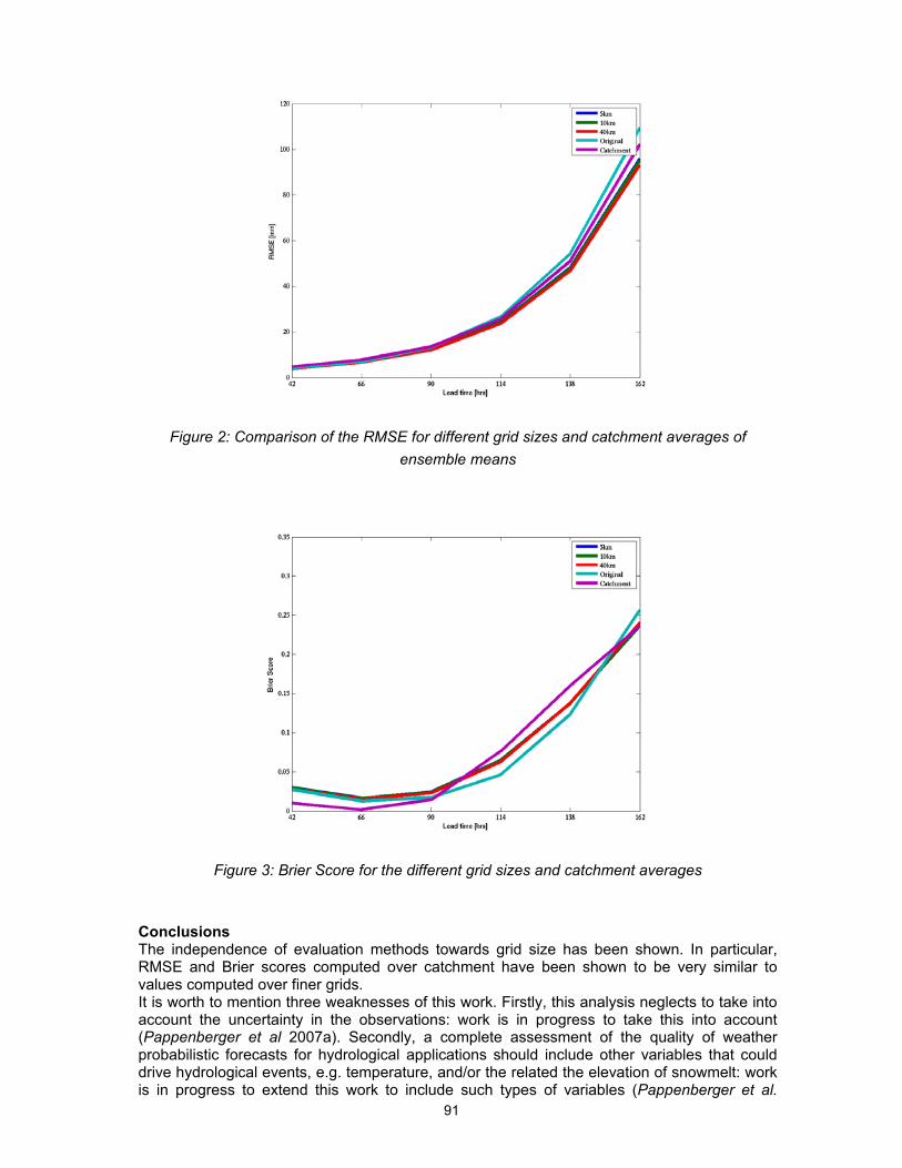
91

Figure 2: Comparison of the RMSE for different grid sizes and catchment averages of ensemble means

Figure 3: Brier Score for the different grid sizes and catchment averages

Conclusions The independence of evaluation methods towards grid size has been shown. In particular, RMSE and Brier scores computed over catchment have been shown to be very similar to values computed over finer grids. It is worth to mention three weaknesses of this work. Firstly, this analysis neglects to take into account the uncertainty in the observations: work is in progress to take this into account (Pappenberger et al 2007a). Secondly, a complete assessment of the quality of weather probabilistic forecasts for hydrological applications should include other variables that could drive hydrological events, e.g. temperature, and/or the related the elevation of snowmelt: work is in progress to extend this work to include such types of variables (Pappenberger et al.

92

2007b). Thirdly, this analysis focused on a very limited period: the plan is to extend it to include other periods to be able to draw stronger (from a statistical point of view) conclusions. Acknowledgements: Florian Pappenberger is funded by the PREVIEW (FP6 - Work Package: Plain Floods) program (http://www.preview-risk.com).

References - Ahrens, B. and Jaun, S., 2007. On evaluation of ensemble precipitation forecasts with observation-based ensembles. Advances in Geosciences, 10: 139-144. - Buizza, R., Bidlot, J.-R., Wedi, N., Fuentes, M., Hamrud, M., Holt, G., & Vitart, F., 2007: The new ECMWF VAREPS. Q. J. Roy. Meteorol. Soc., in press. - Buizza, R., Pappenberger, F. et al., 2007. Technical and functional quality, and forecast value of meterological and hydrological predictions. Hydrological Sciences Bulletin-Bulletin Des Sciences Hydrologiques: in preparation - de Roo, A. et al., 2003. Development of a European Flood Forecasting System. International Journal of River Basin Management, 1: 49-59. - Ghelli, A. and Lalaurette, F., 2000. Verifying precipitation forecasts using up-scaled observations. ECMWF Newsletter, 87: 9-17. - Gouweleeuw, B., Thielen, J., de Roo, A. and Buizza, R., 2005. Flood forecasting using probabilistic weather predictions. Hydrology and Earth System Science, 9(4). - Jolliffe, I.T. and Stephenson, D.B., 2003. Forecast verification : a practitioner's guide in atmospheric science. J. Wiley, Chichester, xiii, 240 p. pp. - Palmer, T.N., 2002. The economic value of ensemble forecasts as a tool for risk assessment: From days to decades. Quarterly Journal of the Royal Meteorological Society, 128(581): 747-774. - Pappenberger, F. et al., 2005. Cascading model uncertainty from medium range weather forecasts (10 days) through a rainfall-runoff model to flood inundation predictions within the European Flood Forecasting System (EFFS). Hydrology and Earth System Science, 9(4): 381-393. - Pappenberger, F., Buizza, R., Bodis, K. and Ghelli, A., 2007a. The skill of probabilistic forecasts under observational uncertainties within the Generalized Likelihood Uncertainty Estimation framework for hydrological applications. in preparation. - Pappenberger, F. et al., 2007b. Comparison and analysis of the July/August 2002 Danube flood, in preparation.

93

An ensemble hydrological forecasting system for the Laurentian Great Lales by A. Pietroniro, V. Fortin*, N. Kouwen, I. Doré, C. Neal, K. Legault, D. Nsengiyumva, E. Klyszejko, R. Turcotte, B. Davison, D. Verseghy, E.D. Soulis, R Caldwell, N. Evora and P. Pellerin

AN ENSEMBLE HYDROLOGICAL FORECASTING SYSTEM FOR THE LAURENTIAN GREAT LAKES Alain Pietroniro1, Vincent Fortin2,*, Nicholas Kouwen3, Isabelle Doré2, Champa Neal4, Karine Legault4, Dominique Nsengiyumva4, Erika Klyszejko4, Richard Turcotte5, Bruce Davison6, Diana Verseghy7, E.D. Soulis3, Rob Caldwell8, Noël Evora9 and Pierre Pellerin2

1 Aquatic Ecosystem Impacts Research Division, Environment Canada 2 Meteorological Research Division, Environment Canada 3 Department of Civil Engineering, University of Waterloo 4 Hydrological Applications and Services, Environment Canada 5 Centre d'expertise hydrique du Québec, Ministère de l'environnement, du développement durable et des parcs, Gouvernement du Québec 6 Hydrometeorology and Arctic Lab, Environment Canada 7 Climate Research Division, Environment Canada 8 Great Lakes and St. Lawrence Regulation Office, Environment Canada 9 Institut de recherche d'Hydro-Québec

* Corresponding author: Canadian Meteorological Centre, 2121 Trans-Canada Highway, 5th floor, Dorval (Québec) Canada H9P 1J3, 1(514)421-4630, vincent.fortin@ec.gc.ca Abstract The MESH surface and hydrological model has been set up on a grid of 1/6th of a degree for the Great Lakes and St. Lawrence basin upstream of Montreal, Quebec, and coupled to the global Canadian ensemble prediction system, to obtain ensemble forecasts of land-surface variables as well as streamflow. Forecasts are issued once a week for a lead-time of two weeks, posted to an anonymous ftp site and verified against observations of snowpack and streamflow. In this paper, we present in more details the setup of the current experiment and then discuss the strengths and weaknesses of the system from the point of view of different users, which leads us to present a number of ways in which the system could be improved in the coming years. 1. Introduction Recent efforts to generate medium-range hydrological ensemble forecasts on large basins by coupling an operational atmospheric ensemble prediction system (EPS) with a regional-scale, raster-based, hydrological model have shown promising results based on case studies (Hou et al., 2007; Pietroniro et al., 2007; Gouweleeuw et al., 2005). However, convincing researchers, forecasters, and end-users that such an ensemble hydrological forecasting system improves upon existing hydrological forecasting systems, and getting them to use such a system, requires more than case studies. One way to build confidence into the system is to conduct a reforecasting experiment, from which a lot of information can be gleaned for a fixed version of an EPS (Hamill et al, 2004; 2006). Another is to start to produce and disseminate experimental ensemble forecasts of future events using a setup that is as close as possible to an operational forecasting system, and initiate a discussion with potential end-users to see if the current setup can already be of any use, or how much better it should get before it becomes useful, and what specific products they would like. In this spirit, the MESH modelling system (Pietroniro et al., 2007) has been set up on a grid of 1/6th of a degree for the Great Lakes and St. Lawrence basin upstream of Montreal, Quebec, and coupled to the global Canadian ensemble prediction system. In this paper, we describe the current configuration of this ensemble hydrological forecasting system, and then discuss concerns and hopes of potential end-users with respect to the future forecasting system.

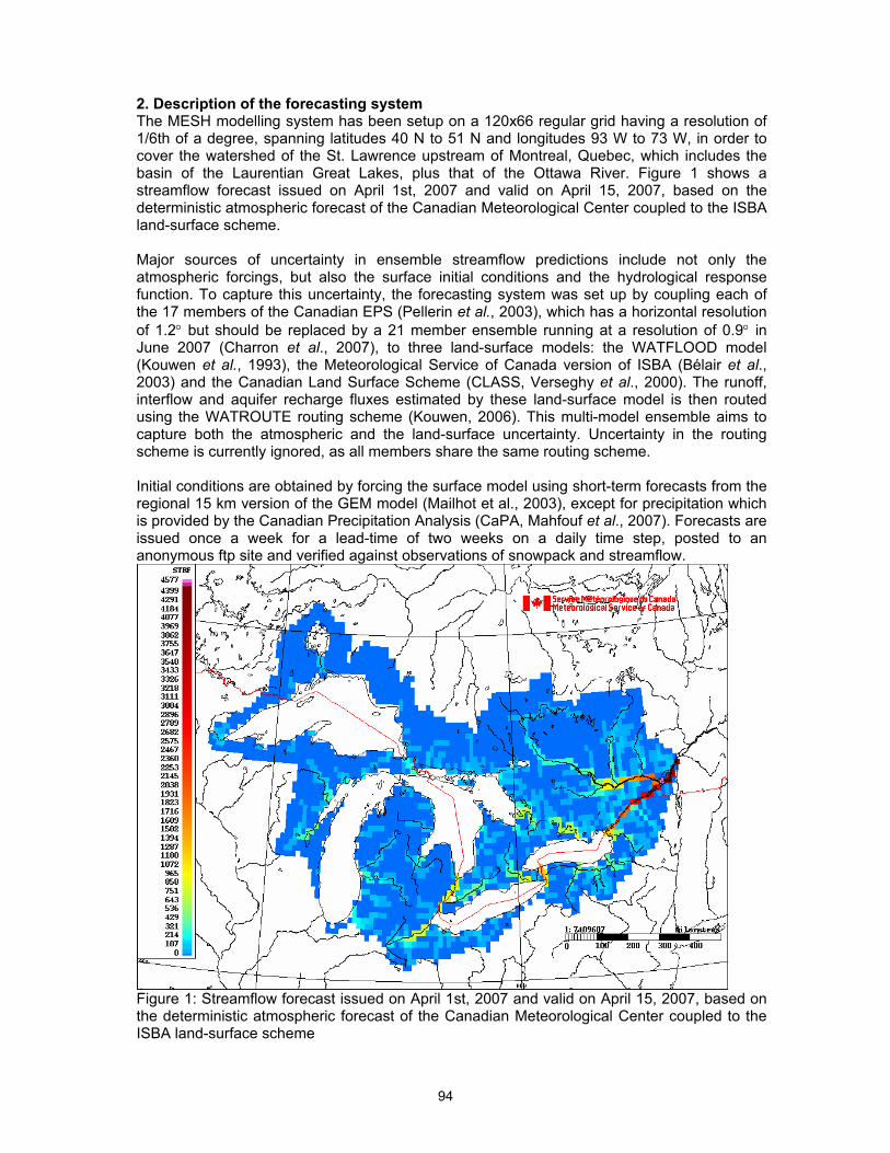
94

2. Description of the forecasting system The MESH modelling system has been setup on a 120x66 regular grid having a resolution of 1/6th of a degree, spanning latitudes 40 N to 51 N and longitudes 93 W to 73 W, in order to cover the watershed of the St. Lawrence upstream of Montreal, Quebec, which includes the basin of the Laurentian Great Lakes, plus that of the Ottawa River. Figure 1 shows a streamflow forecast issued on April 1st, 2007 and valid on April 15, 2007, based on the deterministic atmospheric forecast of the Canadian Meteorological Center coupled to the ISBA land-surface scheme. Major sources of uncertainty in ensemble streamflow predictions include not only the atmospheric forcings, but also the surface initial conditions and the hydrological response function. To capture this uncertainty, the forecasting system was set up by coupling each of the 17 members of the Canadian EPS (Pellerin et al., 2003), which has a horizontal resolution of 1.2° but should be replaced by a 21 member ensemble running at a resolution of 0.9° in June 2007 (Charron et al., 2007), to three land-surface models: the WATFLOOD model (Kouwen et al., 1993), the Meteorological Service of Canada version of ISBA (Bélair et al., 2003) and the Canadian Land Surface Scheme (CLASS, Verseghy et al., 2000). The runoff, interflow and aquifer recharge fluxes estimated by these land-surface model is then routed using the WATROUTE routing scheme (Kouwen, 2006). This multi-model ensemble aims to capture both the atmospheric and the land-surface uncertainty. Uncertainty in the routing scheme is currently ignored, as all members share the same routing scheme. Initial conditions are obtained by forcing the surface model using short-term forecasts from the regional 15 km version of the GEM model (Mailhot et al., 2003), except for precipitation which is provided by the Canadian Precipitation Analysis (CaPA, Mahfouf et al., 2007). Forecasts are issued once a week for a lead-time of two weeks on a daily time step, posted to an anonymous ftp site and verified against observations of snowpack and streamflow.

Figure 1: Streamflow forecast issued on April 1st, 2007 and valid on April 15, 2007, based on the deterministic atmospheric forecast of the Canadian Meteorological Center coupled to the ISBA land-surface scheme

95

3. All models are wrong. Is this one useful? Preliminary results indicate that the forecasting system has some skill at predicting snow water equivalent and streamflow (Pietroniro et al., 2007). In order to evaluate whether the forecasts could actually be useful to forecasters, we have had informal discussions with hydrological forecasters working for agencies responsible for managing different subwatersheds on the basin. One of the largest hydropower producers on the basin is Hydro-Québec, which operates power plants on the St. Lawrence river as well as power plants and reservoirs on the Ottawa River, is very interested by two-week ensemble forecasts, provided that they are proven to be skillful and reliable and have a low false-alarm ratio. Because we have yet to conduct a reforecasting experiment, we cannot at the moment assess the reliability and false-alarm ratio of the system. At the Great Lakes and St. Lawrence Regulation Office, a Canadian agency which provides forecasts of lake levels and lake outflows to the International St. Lawrence River Board of Control and to the International Lake Superior Board of Control, the focus is on monthly to seasonal time scale. Consequently, two-week ensemble forecasts are not sufficient to meet their needs. As the meteorological ensemble forecasts already have little skill for week two, it does not make sense to extend the lead-time of the atmospheric ensemble prediction system to meet their needs, but monthly inflows forecasts to the lakes could still be obtained by relaxing the atmospheric forcings to climatology after two weeks, assuming that there is still information in the land-surface or lake initial conditions. Monthly forecasts would also be useful for the Canadian Department of Fisheries and Oceans (DFO), which issues forecasts of water levels in the St. Lawrence River for navigation planning purposes. This would also require coupling the hydrological model to an existing hydraulic model of the St. Lawrence River, as it is under oceanic tidal influence. DFO also issues 48h forecasts of water levels for navigation safety, and would thus be interested in hydrological forecasts which reflect the uncertainty in short-term atmospheric forecasts, something that the current system does not do. Organizations which issue forecasts for flood warning and for managing small dams on the system, such as the Centre d'Expertise Hydrique du Québec, also would like the ensemble forecasting system to better reflect meteorological uncertainty in the first 48h, as they mainly act upon short-term forecasts. 4. Improving the forecasting system to meet users' demands In order to try to meet users' demands, we plan to modify the system in order to be able to eventually offer 3-hourly ensemble forecasts for the first 48h, daily forecasts for the first week, and weekly forecasts for the first four weeks. In order to represent the uncertainty in short-term forecasts, we will rely on the future Canadian regional ensemble prediction system, which will have a horizontal resolution of 33 km and a lead-time of 48h (Li et al., 2006), whereas we will plan to use climatological scenarios to force the model for weeks 3 and 4. A good estimation of surface initial conditions and of the associated uncertainty is very important for short lead-time and seasonal hydrological forecasts, in the first case because the meteorological uncertainty is smaller than for medium-range forecasts, in the second case because there is little skill left in the meteorological forcing. It will therefore be important to focus our efforts on improving the land-surface, lake, and routing models. This will be achieved by improving modelling of subgrid processes in the land-surface model, including a thermodynamic lake and ice model for subgrid lakes and large lakes, improving the calibration of the routing model on observed streamflow, and coupling to existing hydraulic models for the main channels.

96

5. Conclusion Setting up an experimental ensemble hydrological forecasting system is an important first step towards making operational dynamical ensemble hydrological forecasting a reality on the Great Lakes and St. Lawrence basin, as experimental forecasts of future events are often more convincing for users that case studies on past events. In particular, it facilitates the dialogue between researchers and end-users, which should help focusing research and development in directions that are likely to help make the system more useful. We are aware that convincing users that the system is skillful and reliable will be difficult without a reforecasting experiment. Given the high cost of performing such an experiment, reforecasting requires sufficient confidence that the forecasting system being evaluated is appropriate for the problem that it addresses, both in terms of skill and in terms of usefulness for water managers. This is exactly what we aim to accomplish with the current forecasting system. References

- Bélair, S., Crevier, L.-P., Mailhot, J., Bilodeau, B., Delage, Y. 2003. Operational Implementation of the ISBA Land Surface Scheme in the Canadian Regional Weather Forecast Model. Part I: Warm Season Results. Journal of Hydrometeorology, 4(2): 352-370.

- Charron, M., Pellerin, G., Spacek, L., Candille, G., Houtekamer, P. 2007. An improved Ensemble Prediction System for operational medium-range weather forecasts at CMC. Canadian Meteorological and Oceanographic Society, May 28th - June 1st, 2007.

- Gouweleeuw, B., Thielen, J., Franchello, G., De Roo, A., Buizza, R. 2005. Flood forecasting using medium-range probabilistic weather prediction. Hydrological and Earth System Sciences, 9(4), pp.365-380.

- Hamill, T.M., Whitaker, J.S., Dole, R.M. 2006. Producing high-skill probabilistic forecasts using reforecasts: implementing the National Research Council vision. NOAA Earth System Research Lab, draft report, 15 august 2006.

- Hamill, T.M., Whitaker, J.S., Wei, X. 2004. Ensemble reforecasting: Improving medium-range forecast skill using retrospective forecasts. Mon. Wea. Rev., 132(6): 1434-1447.

- Hou, D., Mitchell, K., Toth, Z., Lohmann, D., Wei, H. 2007. Ensemble river forecasting experiments at NCEP. Geophysical Research Abstracts, 9: 11123.

- Li, X., Charron, M., Spacek, L., Candille, G. 2006. A regional ensemble prediction system based on moist targeted singular vectors and stochastic parameter perturbations. Monthly Weather Review, submitted for publication.

- Kouwen, N., Soulis, E.D., Pietroniro, A., Donald, J., Harrington, R.A. 1993. Grouping Response Units for Distributed Hydrologic Modelling. J. Wat. Res. Plan. Man., 119(3):289-305.

- Kouwen, N. 2006. WATFLOOD/WATROUTE hydrological model routing & flow forecasting system, University of Waterloo.

- Mahfouf, J.-F., Brasnett, B., Gagnon, S. 2007. A Canadian precipitation analysis (CAPA) project. Description and preliminary results. Atmosphere-Ocean, 45(1): 1-17.

- Mailhot J., Bélair, S., Lefaivre, L., Bilodeau, B., Desgagné, M., Girard, C., Glazer, A., Leduc, A.-M., Méthot, A., Patoine, A., Plante, A., Rahill, A., Robinson, T., Talbot, D., Tremblay, A., Vaillancourt, P., Zadra, A., Qaddouri, A. 2006. The 15-km version of the Canadian regional forecast system. Atmosphere-Ocean, 44(2): 133-149.

- Pietroniro, A., Fortin, V., Kouwen, N., Neal, C., Turcotte, R., Davison, B., Verseghy, D., Soulis, E.D., Caldwell, R., Evora, N., Pellerin, P. 2007. Using the MESH modelling system for hydrological ensemble forecasting of the Laurentian Great Lakes at the regional scale. Hydrological and Earth System Sciences, 11: 1279-1294.

- Pellerin, G., Lefaivre, L., Houtekamer, P., Girard, C. 2003. Increasing the horizontal resolution of ensemble forecasts at CMC, Nonlinear Processes in Geophysics, 10:463-468.

- Verseghy, D. L. 2000. The Canadian Land Surface Scheme (CLASS): its history and future. Atmosphere-Ocean, 38(1): 1-13.

97

Q-R

EFAS EPS based forecasts: in-depth case study analyses and statistical evaluation of summer 2005 and sprink 2006 flood forecasts by M.H. Ramos, J. Thielen and J. Bartholmes EFAS EPS-based forecasts: in-depth case study analyses and statistical evaluation of summer 2005 and spring 2006 flood forecasts Maria-Helena Ramos1,2,*, Jutta Thielen1, Jens Bartholmes1

1 European Commission, DG Joint Research Centre, Institute for Environment and Sustainability, TP261, 21020 Ispra (Va), Italy. 2 Cemagref Lyon, Hydrology and Hydraulics Research Unit, France. * Corresponding author: 3 bis quai Chauveau, CP 220 - 69336 LYON Cedex 09 – France, Tél. +33 (0) 4 72 20 87 65 - FAX : +33 4 78 47 78 75, e-mail : ramos@lyon.cemagref.fr Abstract This study deals with the analysis and interpretation of case studies in view to defining rules to an objective and statistical evaluation of ensemble flood forecasts from the European Flood Alert System (EFAS). First, we investigate EFAS forecasts on a flood-event basis. The aim is to investigate the ability of EFAS flood forecasts based on Ensemble Prediction System (EPS) to provide earlier warning, comparatively and/or complementarily to the forecasts based on deterministic weather forecasts. Secondly, a statistical analysis of the flood events forecasted over the flood-prone periods of summer 2005 and spring 2006 is performed. The analysis focuses on i) the statistical evaluation of hits, misses and false alarms as a function of the number of EPS-based simulations exceeding a given EFAS flood alert threshold and ii) on the comparative analysis of gain in preparedness (early forecasting) when operational alert rules are applied on both forecasts based on probabilistic and deterministic weather forecasts to define a potential flooding situation. The analyses were performed over a number of representative points selected throughout the Danube and the Elbe river basins. 1. Introduction The use of meteorological ensemble prediction systems (EPS) coupled with hydrologic models for probabilistic flood forecasting and risk assessment is a novelty and a challenge for the scientific community and for decision makers dealing with operational flood forecasting (Krzysztofowicz, R., 2001; Moore et al., 2006). The European Flood Alert System (EFAS) is a European-wide integrated hydro-meteorological platform offering a suitable framework to explore the use of state-of-the-art meteorological products as weather ensembles in hydrological forecasting under different climatic and geographic conditions. The first attempt to visualize simulated discharges based on ECMWF-EPS weather forecasts within the EFAS framework was performed by Gouweleeuw et al. (2005) during the European EFFS research project (De Roo et al., 2003, Thielen, 2004). It prompted the development of new products, which were implemented in early summer 2005 in the first EFAS prototype. Maps showing the number of EPS-based simulations exceeding pre-defined EFAS flood thresholds and temporal box diagrams of forecasted exceedances at a given point in a river were implemented in order to provide a clear view of the ensemble predictions in space and time. Combined forecast diagrams were developed to allow a complementary visualisation of EFAS deterministic- and probabilistic-based forecasts all together (Thielen et al., 2006; Ramos et al., 2006). The development of these products was conducted in close collaboration with the users of EFAS forecasts (the national operational flood forecasting services), which found them useful when analyzing a potential flood situation (Thielen et al., 2005). In this study we investigate EFAS performance for individual flood events observed in European catchments in order to get a better understanding of the strengths and limitations on the use of EPS in EFAS ensemble flood forecasts. We investigate the appropriate rules for an objective assessment of the quality of flood forecasts, as well as the ability of the system to provide earlier warning from combined (deterministic and probabilistic) flood forecasts. 2. Methodology

98

We investigate EFAS forecasts based on the meteorological Ensemble Prediction System (EPS) of the European Centre for Medium-Range Weather Forecasts (ECMWF). In this study, the 10-day ECMWF EPS is characterized by 50 perturbed members and 1 control run, with about 80-km grid spacing at mid latitudes (Molteni et al., 1996; Buizza et al., 2001). The study is performed at river locations in the Danube and the Elbe river basins, which were the European basins most affected by floods in 2005-2006. The selected points are associated with a wide range of upstream areas, from 1,000 km2 to 660,000 km2. The study is performed on i) a flood-event basis and ii) a seasonal basis (summer 2005 and spring 2006). For selected flood events, historical EFAS forecast diagrams at affected locations were built and forecasted flood threshold exceedances were compared to exceedances obtained from a proxy for observed discharges. The proxy consists of simulated discharges using observed meteorological data as input and the same hydrologic model and setup applied in the forecasting system. These post-event analyses are a necessary step to understand the potential capabilities of the forecasting system to capture different types of flood events. They also allow to identify interpretation and decision rules to better define alert situations that produce meaningful early flood alerts, with a small number of false alarms and a reduced number of missed events. On a seasonal basis, the analysis was performed on a larger number of locations and over long time periods (summer 2005 and spring 2006). The analysis comprises i) the evaluation of hits, misses and false alarms and ii) the comparative analysis of gain in preparedness (early forecasting) when operational alert rules are applied on both forecasts based on probabilistic and deterministic weather forecasts to define a potential flooding situation. First, hits, misses and false alarms are determined in the EFAS forecast diagrams. For the hits and misses definition, observed events are considered if discharges simulated with observed meteorological data as input (proxy for observed discharges) exceed EFAS high flood threshold. A forecasted event is flagged when there is persistence of the forecasted signal according to the following rules: i) for the deterministic-based forecasts: forecasted discharges exceed EFAS high flood threshold in two consecutive simulations based on weather forecasts issued at 12UTC; ii) for the probabilistic EPS-based forecasts: forecasted discharges exceed EFAS high flood threshold in two consecutive simulations based on weather forecasts issued at 12UTC, both with Nth or more EPS simulations above EFAS high flood threshold (Nth ranges from 1 to 50). Secondly, the gain (or loss) in preparedness for EPS-based forecasts, comparatively to deterministic-based forecasts, is calculated when there is an observed event and for each Nth defined above. It is evaluated by taking the difference between the lead time associated with the first signal in EFAS EPS-based forecast and the lead time associated with the first signal in EFAS deterministic-based forecast. If the difference is negative, a hit was forecasted earlier by ECMWF deterministic or a hit was forecasted by ECMWF, while EPS simulations indicated a miss. If the difference is positive, a hit was forecasted earlier by EPS simulations or a hit was forecasted by EPS simulations, while ECMWF deterministic simulations indicated a miss. 3. Results The main results of this study are summarized below. • The in-depth analysis of case-studies proved to be very useful in understanding the behaviour of EFAS forecasts under different hydro-meteorological conditions. They were also essential to the definition of appropriate rules for an objective assessment of EFAS performance over long time periods and on European scale. • The importance of defining a criterion of persistence in forecasts of consecutive days, together with a criterion of consistence between different forecasts at the same forecast date, for EFAS to flag a possible flooding event was highlighted.

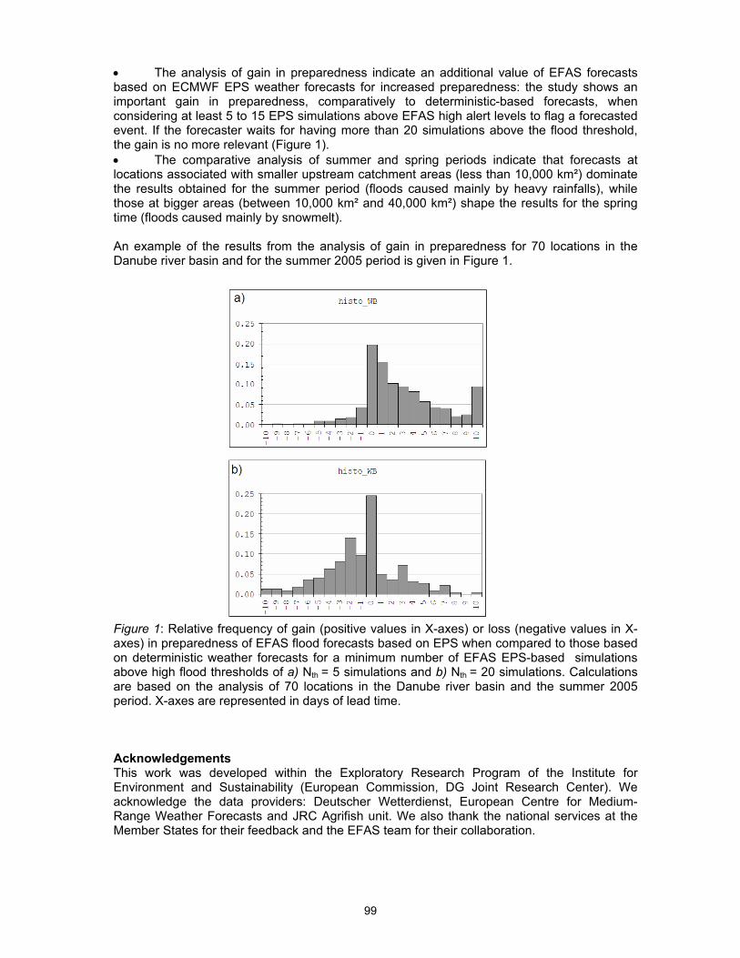
99

• The analysis of gain in preparedness indicate an additional value of EFAS forecasts based on ECMWF EPS weather forecasts for increased preparedness: the study shows an important gain in preparedness, comparatively to deterministic-based forecasts, when considering at least 5 to 15 EPS simulations above EFAS high alert levels to flag a forecasted event. If the forecaster waits for having more than 20 simulations above the flood threshold, the gain is no more relevant (Figure 1). • The comparative analysis of summer and spring periods indicate that forecasts at locations associated with smaller upstream catchment areas (less than 10,000 km²) dominate the results obtained for the summer period (floods caused mainly by heavy rainfalls), while those at bigger areas (between 10,000 km² and 40,000 km²) shape the results for the spring time (floods caused mainly by snowmelt). An example of the results from the analysis of gain in preparedness for 70 locations in the Danube river basin and for the summer 2005 period is given in Figure 1.

Figure 1: Relative frequency of gain (positive values in X-axes) or loss (negative values in X-axes) in preparedness of EFAS flood forecasts based on EPS when compared to those based on deterministic weather forecasts for a minimum number of EFAS EPS-based simulations above high flood thresholds of a) Nth = 5 simulations and b) Nth = 20 simulations. Calculations are based on the analysis of 70 locations in the Danube river basin and the summer 2005 period. X-axes are represented in days of lead time. Acknowledgements This work was developed within the Exploratory Research Program of the Institute for Environment and Sustainability (European Commission, DG Joint Research Center). We acknowledge the data providers: Deutscher Wetterdienst, European Centre for Medium-Range Weather Forecasts and JRC Agrifish unit. We also thank the national services at the Member States for their feedback and the EFAS team for their collaboration.

100

References - Buizza, R., Richardson, D.S. & Palmer, T.N., 2001. The new 80-km high-resolution

ECMWF EPS. ECMWF Newsletter 90: 2-9. - De Roo, A., Gouweleeuw, B., Thielen, J., Bates, P., Hollingsworth, A. et al., 2003.

Development of a European Flood Forecasting System. International Journal of River Basin Management 1(1): 49-59.

- Gouweleeuw, B., Thielen, J., Franchello, G., De Roo, A., Buizza, R., 2005. Flood forecasting using medium-range probabilistic weather prediction. Hydrological and Earth System Sciences, 9(4): 365-380.

- Krzysztofowicz, R., 2001. The case for probabilistic forecasting in hydrology. Journal of Hydrology 249: 2-9.

- Molteni, F., Buizza, R., Palmer, T.N. & Petroliagis, T., 1996. The ECMWF ensemble prediction system: methodology and validation. Q.J.R. Meteorological Society, 122(529): 73-119.

- Moore, R.J., Cole, S.J., Bell, V.A., Jones, D. A., 2006. Issues in flood forecasting: ungauged basins, extreme floods and uncertainty. IAHS Publ. 305, Frontiers in Flood Research, Kovacs Colloquium UNESCO, Paris, June/July 2006, p. 103-122.

- Ramos M-H., Bartholmes J., Thielen J., Kalas M., de Roo A., 2006. The additional value of ensemble weather forecasts to flood forecasting: first results on EFAS forecasts for the Danube River Basin. Proceedings of the XXIII Conference of the Danubian Countries on the Hydrological Forecasting and Hydrological Bases of Water Management, 28-31 August 2006, Belgrade, Republic of Serbia, CD-ROM, 12p.

- Ramos, M.H., 2006. EFAS-EPS forecasts: in-depth case study analyses and statistical evaluation of summer 2005 and spring 2006 flood forecasts in the Danube catchment. In: Thielen, J. (ed.): The benefit of probabilistic flood forecasting on European scale - Results of the European Flood Alert System for 2005/2006. European Commission, EUR 22560EN, Chapter 4: 36-58.

- Thielen J, Ramos, M.H., Bartholmes, J., De Roo, A., Cloke, H., Pappenberger, F., Demeritt, D., 2005. Summary report of the 1st EFAS workshop on the use of Ensemble Prediction System in flood forecasting, 21-22nd November 2005, Ispra. European Commission, EUR 22118EN, 23p.

- Thielen J., 2004. Flood forecasting results: Europe. In: Gouweleeuw, B., Reggiani, P. & de Roo. A. (ed.): A European Flood Forecasting System EFFS. Full Report, European Commission, EUR 21208 EN, p.187-197.

- Thielen J., Bartholmes J., Ramos M-H., Kalas M., van der Knijff J. & de Roo A., 2006. Added value of ensemble prediction system products for medium-range flood forecasting on European scale. In: Proceedings of the workshop “Ensemble Predictions and Uncertainties in Flood Forecasting”, International Commission for the Hydrology of the Rhine Basin (CHR), Bern Switzerland, 30-31 March 2006, p.77-82.

101

The Map D-Phase operations period (DOP) by M. W. Rotach and M. Arpagaus

The MAP D-PHASE operations period (DOP) Mathias W. Rotach and Marco Arpagaus Swiss Federal Office of Meteorology and Climatology (MeteoSwiss), Zürich, Switzerland Manfred Dorninger, Univerity of Vienna, Vienna, Austria Christoph Hegg, WSL, Birmensdorf, Switzerland Andrea Montani, ARPA-SIM, Bologna, Italy Roberto Ranzi, Unversity of Brescia, Italy D-PHASE (Demonstration of Probabilistic Hydrological and Atmospheric Simulation of flood Events in the alpine region) is a WWRP (World Weather Research Programme) Forecast Demonstration Project related to the Mesoscale Alpine Programme (MAP). It focuses on the demonstration of, ability and improvement in forecasting (heavy) precipitation events and related flooding in the Alps. In that sense it covers high-resolution numerical modelling, ensemble forecasting, hydrological modelling and Nowcasting, including radar techniques. The actual demonstration period of MAP D-PHASE (DOP), is from June to November 2007, encompassing the ‘classical’ MAP period (September – November) as well as the Convective and Orographically-induced Precipitation Study (COPS) observations programme (June – August). Thus at the time of the HEPEX workshop, the DOP is only one month ‘old’. The Project will briefly be presented by introducing its goals and scientific environment. Further, we will illustrate on the example of the actual meteorological development what products and possibilities are available in the entire forecasting chain ranging from limited-area ensemble forecasting, high-resolution atmospheric modelling (km-scale), hydrological modelling (including ensemble hydrological modelling), and nowcasting to decision making by the end users, i.e., the entire end-to-end flood forecasting system. First experience from the dry runs (which are not necessarily ‘dry’ in terms of precipitation) as well as from the tests on high-resolution verification (that will be a major undertaking in the aftermath of the DOP – done on MAP cases) will be presented as well.

102

S-T

Assessment of bias removal for deterministic medium-range weather forecasts in the Po river basin, Italy, Europe by Salamon, P., and Thielen, J.

Assessment of bias removal for deterministic medium-range weather forecasts in the Po river basin, Italy, Europe Salamon, P., and Thielen, J. European Commission, DG Joint Research Centre, Institute for Environment and Sustainability, TP261, 21020 Ispra (Va), Italy. Email: peter.salamon@jrc.it Abstract The quality of medium-range flood forecasting depends strongly on the meteorological forecasting data used to drive the hydrological model. However, numerical weather prediction (NWP) models can contain significant systematic error especially with respect to precipitation leading to an over/under-forecasting of flooding events. A variety of different bias-correction methods exists to remove these systematic errors from the NWP models. In this work we will evaluate the efficiency of a running median bias correction approach for precipitation forecasts. As a first step the bias in the forecast data for a four year time period from 01/2003 to 12/2006 was analyzed using a high-density observing network for the Po river basin. The different leadtimes of the DWD and ECMWF deterministic models were examined and it was found that the over or under representation of precipitation is strongly spatially dependant. Neither a general over/under-forecasting nor seasonal trends could be observed for the precipitation forecasts in the Po river basin. The spatial and temporal variability of the systematic error requires a bias correction method capable of addressing these aspects. Furthermore, as this method will be applied to a daily operational flood forecasting system, the approach needs to be easy to implement and computationally efficient. Currently, time lengths of 7, 10, 14, 20, and 30 days for the running median bias correction are evaluated using the well-known forecast verification scores. However, as comparing observed precipitation data with forecasts can lead to misinterpretations due to the different spatial scales of the data, the bias-corrected forecasts are furthermore validated using runoff measurements obtained by coupled atmospheric hydrological simulations.

103

Statistical re-scaling and downscaling testbed project: status reportby J. Schaake

STATISTICAL RE-SCALING AND DOWNSCALING TESTBED PROJECT: STATUS REPORT John Schaake, Consultant, NOAA NWS Office of Hydrologic Development Silver Spring, MD john.schaake@noaa.gov Project Purpose Scientific Question What are the advantages and limitations of different methods for extracting information from Numerical Weather Prediction models for the purposes of forecasting streamflow? Objective(s) • Identify the space-time scales for which forecast skill is present, for different variables, and develop methods to extract and combine information at different space-time scales • Identify the atmospheric forecast variables that can be used to provide sub-grid information—for example, wind and humidity output can be used in a statistical model to replicate orographic precipitation processes, and provide local-scale information that is not present in the raw precipitation output [Clark and Hay (2004) have a table that summarizes the frequency that different variables are used in their regression equations]. • Identify of the sample size required to reliably forecast precipitation, temperature, and streamflow, for different thresholds. Accomplishments Background Hydrologic forecast models are highly non-linear. As a result they are very sensitive to biases in the climatology of input forcing, especially precipitation forcing, as well as biases in the spread of ensemble forecasts of input forcing. Because hydrologic models integrate the effects of input forcing in time and space, joint distribution properties of input forcing between different times and places are important. Hydrologic models are also sensitive to covariance properties as well as variance properties of the input forcing. Covariance properties are scale dependent in space and time. Hydrologic sensitivity to bias and variability to input forcing is important for all forecast lead times, including flash flood time scales. It also is important for analyzed forcing used in hydrologic simulation as well as future forcing used in hydrologic forecasting. There are two fundamental problems in using information from atmospheric forecasts to create input forcing data sets for hydrologic prediction. One is that there is a scale miss-match between the spatial scales at which atmospheric models operate and spatial scales at which hydrologic models operate. Typically atmospheric models operate at larger spatial scales than the computational scale of hydrologic models. As a result variables such as precipitation that are highly variable in both space and time do not have the same variability characteristics as are required by hydrologic models. In addition, the local climatology of atmospheric models typically is biased relative to the observed local climatology. As a result, atmospheric forecasts must be both re-scaled and downscaled to be most useful for hydrologic prediction. Research on how to assure that forecast information from atmospheric forecast models is used well to create input forcing for hydrologic models is in its infancy. For example, there is a long history of work done to understand the nature of precipitation variability in space and time. But there is a wide gap between that work and the work that is needed to re-scale and downscale precipitation forecasts for hydrologic application.

104

The work that has been done for this test bed so far has focused on building an initial, “reference” ensemble preprocessor for use by the National Weather Service to create ensemble precipitation and temperature forcing for input to its Ensemble Streamflow Prediction (ESP) system. Much of this work has built on earlier work on this problem (Clark and Hay, 2004; Clark et al., 2004; Werner et al, 2005). NWS Ensemble PreProcessor Development One of our main accomplishments has been to develop procedures to use ensemble mean precipitation and temperature forecasts from a fixed version of the National Weather Service (NWS) Global Forecast System (GFS) to produce ensemble forcing for input to hydrologic forecast models at the space and time scales at which the models operate. These procedures were implemented in a prototype operational pre-processing system that is running in an experimental mode at the California Nevada River Forecast Center (CNRFC). These preprocessor procedures are part of what is called the “GFS Subsystem”. The GFS Subsystem allow use of both short and medium range single-value forecasts to produce ensemble forecasts for specific hydrologic basin areas. These procedures are operating at several pilot locations at the CNRFC. Earlier versions of the preprocessor that operate only for very short range forecasts are operating at the Arkansas Basin River Forecast Center (ABRFC) and the Middle Atlantic River Forecast Center (MARFC). An article describing the procedures used in the GFS Subsystem has been submitted for publication in a special issue of the European Geophysical Union’s (EGU) Hydrology and Environmental Sciences (HESS) journal. (Schaake et al, 2006). These procedures require an historical archive of single-value forecasts and corresponding observations. A fixed version of NCEP’s GFS ensemble forecast system was used by the NOAA Climate Diagnostic Center (now part of the Earth System Research Laboratory (ESRL) as part of the Physical Sciences Division of NOAA’s Office of Ocean and Atmospheric Research (OAR)) to make ensemble reforecasts from 1979 to date (Hamill et al, 2006; Hamill et al, 2004). The reforecast data as well as current forecasts can be found at http://www.cdc.noaa.gov/reforecast/. These data were used to create an archive of ensemble mean forecasts of precipitation and temperature. The archive of corresponding observations was available for the RFC forecast basin segments at each RFC. Because atmospheric ensemble forecasts do not reliably estimate the conditional uncertainty (i.e. the spread is typically underestimated), only the ensemble mean forecast is used at the present stage of preprocessor development. Empirical statistical relationships between the single-value forecasts and the corresponding observations are used to account for uncertainty and to control the generation of ensemble members. It was found that the uncertainty in the forecasts depends on the duration of the forecast time window (starting at some lead time after the forecast is created and ending Supporting Data Set Development In order to encourage potential research community participation in the activities of this test bed, the data sets being used by NWS to develop its preprocessor procedures are available via anonymous ftp. This includes: (i) an archive of GFS ensemble mean forecasts and (ii) an archive of corresponding observations. Documentation of the supporting data sets is located at ftp://hydrology.nws.noaa.gov/pub/gcip/hepex/documentation/ GFS Ensemble mean Forecast Archive Historical ensemble mean precipitation and temperature forecasts from the fixed version of NCEP’s GFS ensemble forecast system are located under the directory ftp://hydrology.nws.noaa.gov/pub/gcip/hepex/gfs_archive/. There are separate subdirectories

105

for precipitation and temperature. In each of these subdirectories there is a file named ensmean.zip that contains the data. The original GFS ensemble forecast data included 15 members. The forecasts were made once a day at 0000z. Twice daily data values for both precipitation and temperature were given for a 15-day lead time (i.e. 30 values for each member). The forecasts were on a global 2.5 x 2.5 degree grid (144 rows and 73 columns). The mean forecast data provided in this directory are for a domain that only covers the U. S. There are 300 grid points in this domain. The location of row and column grid point centroids and the corresponding grid element indices in the global grid are given in the file gfs_fcst_data.doc in the HEPEX/documentation/ directory. The precipitation and temperature directories contain a file for each grid point. There is a record in each file for each forecast day. The date in the forecast record is the date the forecast was created. Precipitation data were aggregated to daily values for the period 12z-12z. (NWS RFC’s operate on a 12z-12z forecast day). So the forecasts are for 14 days. There are 14 precipitation forecast values and 28 temperature forecast values. Precipitation units are mm. Temperature units are degrees Celsius. Observations Data Archive Historical 6hr Mean Areal Precipitation (MAP) values for more than 430 U.S. river basins are located in directory ftp://hydrology.nws.noaa.gov/pub/gcip/hepex/gfs_archive/mopex/US_Data/6hr_MAP/z12_z12/ascii/. These river basins are being used in the Model Parameter Estimation Experiment (MOPEX) (Schaake et al, 2006). The locations of these basins and information about the USGS stream gages are located in the subdirectory gage locations are in /mopex/basin_characteristics/. Documentation about the preparation of the data and availability of all of the MOPEX data can be found in /mopex/documentation/. The date stamp on these data are for the day on which the valid 12z-12z period ends. Historical mean areal daily precipitation data and max/min temperature data for more than 430 U.S. MOPEX basins are located in the directory ftp://hydrology.nws.noaa.gov/pub/gcip/mopex/us_data/us_438_daily. These data are on a local 24hr clock. As a result the daily precipitation data are out of phase with the daily GFS 12z-12z precipitation data. Therefore the 6hr MAP data described above should be used with the GFS precipitation forecasts. But the daily max min temperature data can be correlated with the 12hr GFS temperature forecasts. Example Results As explained in section 2.2 above an article describing the procedures used in the GFS Subsystem has been submitted for publication in a special issue of the European Geophysical Union’s (EGU) Hydrology and Environmental Sciences (HESS) journal. (Schaake et al, 2006). This article presents selected results for an application of the procedures to the North Fork of the American River basin in California. An example result presented in that publication is presented here. Two different sources of precipitation forecasts for lead times out to 5 days were analyzed. These sources were short-term, single-value forecasts produced by the River Forecast Center (RFC) using a wide range of operational forecast guidance products. The other was the ensemble mean forecast of precipitation from a fixed version of the GFS ensemble forecast system. One of the summary verification statistics used to analyze the results is the continuous rank probability skill score (CRPSS). More about this verification statistic can be found in the paper. But the statistic was applied to each of the two the raw single value forecasts and to ensemble forecasts generated by the EPP for each of them. This was applied to forecasts for 6hr periods out to 5-days (20 periods) plus an additional set of 8 periods were created by accumulating precipitation for different aggregate forecast periods during the 5-day forecast window (see Schaake et al, 2006). This was applied for re-forecasts made during a 5-year period and for all days of the year. The values of the CRPSS are presented in Figure 1

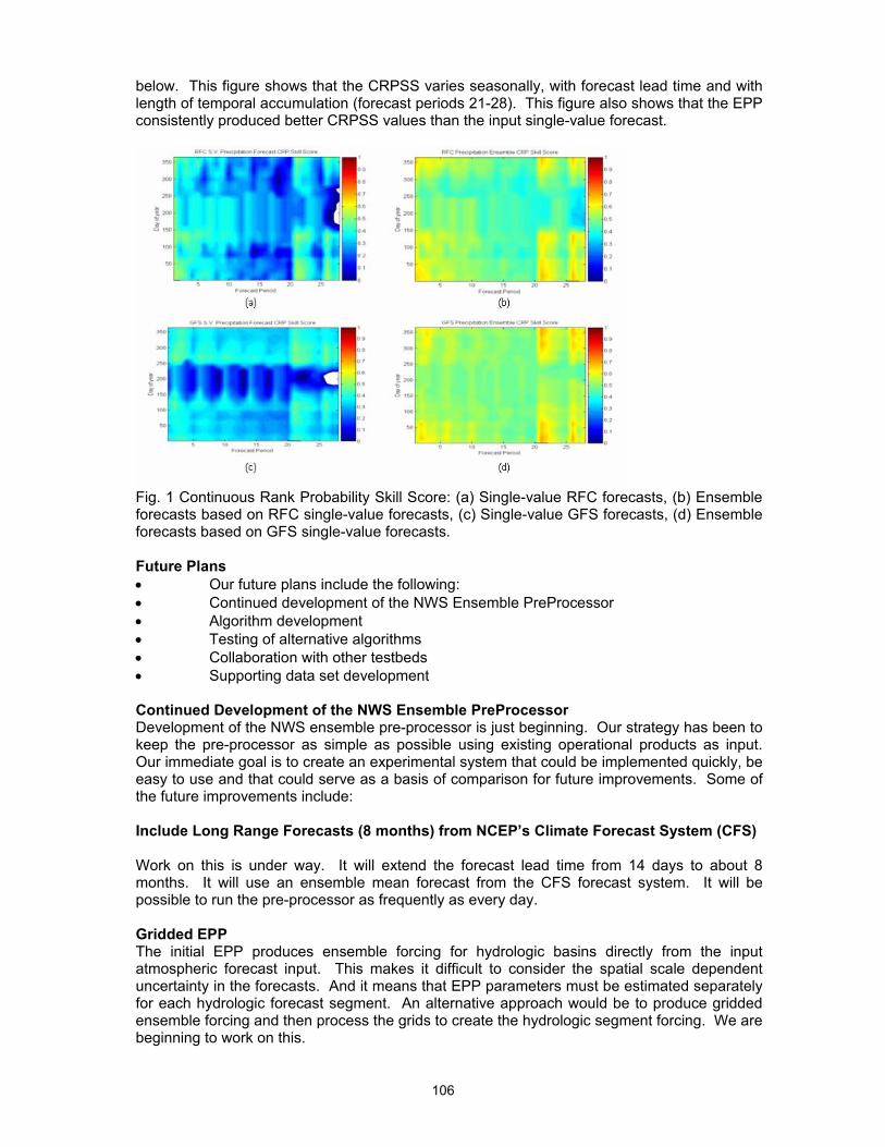
106

below. This figure shows that the CRPSS varies seasonally, with forecast lead time and with length of temporal accumulation (forecast periods 21-28). This figure also shows that the EPP consistently produced better CRPSS values than the input single-value forecast.

Fig. 1 Continuous Rank Probability Skill Score: (a) Single-value RFC forecasts, (b) Ensemble forecasts based on RFC single-value forecasts, (c) Single-value GFS forecasts, (d) Ensemble forecasts based on GFS single-value forecasts. Future Plans • Our future plans include the following: • Continued development of the NWS Ensemble PreProcessor • Algorithm development • Testing of alternative algorithms • Collaboration with other testbeds • Supporting data set development Continued Development of the NWS Ensemble PreProcessor Development of the NWS ensemble pre-processor is just beginning. Our strategy has been to keep the pre-processor as simple as possible using existing operational products as input. Our immediate goal is to create an experimental system that could be implemented quickly, be easy to use and that could serve as a basis of comparison for future improvements. Some of the future improvements include: Include Long Range Forecasts (8 months) from NCEP’s Climate Forecast System (CFS) Work on this is under way. It will extend the forecast lead time from 14 days to about 8 months. It will use an ensemble mean forecast from the CFS forecast system. It will be possible to run the pre-processor as frequently as every day. Gridded EPP The initial EPP produces ensemble forcing for hydrologic basins directly from the input atmospheric forecast input. This makes it difficult to consider the spatial scale dependent uncertainty in the forecasts. And it means that EPP parameters must be estimated separately for each hydrologic forecast segment. An alternative approach would be to produce gridded ensemble forcing and then process the grids to create the hydrologic segment forcing. We are beginning to work on this.

107

Additional Algorithms The initial algorithms were chosen because they were simple, parsimonious with parameters that could be estimated with limited data, even for arid areas. Potentially better algorithms might include: explicit estimation of the probability of precipitation, analog techniques, alternative scale dependency procedures, procedures to use individual members from the atmospheric ensemble forecasts to account for the conditional uncertainty (existing procedures produce the same uncertainty for a given day of the year that is independent of uncertainty estimates available the atmospheric forecast information for that day), procedures to integrate information from multiple forecast models and procedures to integrate long-range empirical statistical forecast information. More careful attention needs to be given to the definition of the probability of precipitation as a function of space and time scale and for precipitation observations/analyses vs precipitation forecasts and to the uncertainty inherent in estimation of the occurrence of precipitation from observations. Verification Statistics We plan to work toward having a unified suite of verification statistics that include summary statistics as well as diagnostic statistics such as found in reliability diagrams and in statistics decompositions that measure effects of bias, resolution and climatological uncertainty. We expect to make progress on this during the coming year. Forecaster Options We plan to consider the possible ways in which the forecaster might control the operation of the EPP. This might include real time control of EPP options, real time diagnostic information about EPP output and possible forecaster over-ride of EPP output. Algorithm Development We will continue to monitor work being done by the international meteorological and hydrological communities on new algorithms. Testing of Alternative Algorithms It is essential that we work to evaluate alternative algorithms and compare alternative algorithms with each other. Ideally this would be done using a common data base and using common metrics. In the near term, the testbed project will do this for algorithms that are being considered for use in the NWS EPP. In the longer run it may be desirable to have a HEPEX intercomparison of alternative EPP algorithms. We plan to pursue this idea first though possible collaboration with other testbeds. But an intercomparison project involving the broader meteorological and hydrological community might be desirable. This is a topic that could be discussed at the 3rd HEPEX workshop in June, 2007. Collaboration with other Testbeds Most of the HEPEX testbeds are using procedures to pre-process atmospheric forecasts before using them as input to their hydrological forecast models. A range of procedures are being used. Some test-beds are developing innovative new and sophisticated procedures. Others are using very basic procedures. In the future we hope to develop plans to test some of these procedures. We also hope to see if any of the work being done by this test-bed would be useful in other testbeds. Supporting Data Set Development We will continue to make data sets that are being used for the development and application of the NWS EPP available to the science community. We are looking forward to working with the WWRP/THORPEX/TIGGEE project to test ensemble forecasts that will be produced by that project. And we look forward to being able to include long range forecasts References, Publications and Presentations

- Clark, M. and L. Hay, 2004,: Use of medium-range weather forecasts to produce predictions of streamflow. Journal of Hydrometeorology, 5, 15-32.

108

- Clark, M., S. Gangopadhyay, L. Hay, B. Rajagopalan, and R. Wilby, 2004: The Schaake Shuffle: a method for reconstructing space-time variability in forecasted precipitation and temperature fields. J. of Hydrometeor., 5 , 243-262.

- Hamill, T. M., J. S. Whitaker, and S. L. Mullen, 2006: Reforecasts: An important dataset for improving weather predictions. Bulletin of the American Meteorological Society, 87, 33-46.

- Hamill, T. M., J. S. Whitaker, and X. Wei, 2004: Ensemble reforecasting: Improving medium-range forecast skill using retrospective forecasts. Mon. Wea. Rev., 132, 1434-1447

- Schaake, J., S. Cong and Q. Duan, 2006: The U. S. MOPEX Data Set, IAHS Red Book #307. - Schaake, J., C., J. Demargne, R. Hartman, M. Mullusky, E. Welles, L. Wu, H. Herr, X. Fan, and

D.J. Seo, 2006: Precipitation and temperature ensemble forecasts from single value forecasts. Hydrology and Earth System Science, hessd-2006-0094.

- Werner, K, D. Brandon, M. Clark and S. Gangopadhay, 2005: Incorporating medium-range numerical weather model output into the ensemble streamflow prediction system of the National Weather Service, J. of Hydrometeor., 5 , 101-114

109

Weather and Society- integrated studies (WAS IS): is the WAS IS initiative relevant to HEPEX? by S. Theis

Weather and society: integrated studies (WAS IS): is the WAS IS initiative relevant to HEPEX? Susanne Theis Deutscher Wetterdienst (DWD), Offenbach, Germany Contact: Susanne.Theis@dwd.de Abstract The HEPEX community is not only interested in the generation of ensemble forecasts, but also in their optimal use. This has led to research questions such as the assessment of user needs or the user's decision making under uncertainty. They can also be viewed as classical research questions within the social sciences. Therefore, HEPEX might benefit from such expertise. However, collaborations with social scientists can be quite difficult, especially if the partners are not prepared for the interdisciplinary challenge. The WAS*IS initiative aims to overcome this barrier and has been establishing a network of meteorologists and social scientists. Within WAS*IS, many user-related questions are already being discussed. Therefore, the WAS*IS network could be a very useful guide to HEPEX in approaching research questions involving the forecast user. 1. Recalling the HEPEX Objectives Part of the HEPEX mission is to “demonstrate how to produce reliable hydrological ensemble predictions that can be used with confidence by emergency management and water resources sectors to make decisions that have important consequences for economy, public health and safety“ (http://hydis8.eng.uci.edu/hepex/). Therefore, HEPEX is not only looking into the generation of ensemble predicitions, but also into their optimal use and their socio-economic benefit. This is also well reflected in many HEPEX workshop discussions which focus on the diversity of user needs, on the communication of uncertainty, on the user's decision making process and on risk assessment. 2. How do HEPEX Objectives Relate to Social Sciences? Within the social sciences, the above-named topics can be viewed as classical research questions. For example, the social sciences have gained rich experience in assessing needs and preferences of certain groups. Psychologists and economists have been extensively looking into “decision making under uncertainty”. Geographers have been looking into “risk assessment“ and they clearly distinguish between exposure, vulnerability, hazard and risk. To carry out a more efficient and scientifically sound analysis of user-related questions within HEPEX, it might be well worth to benefit from social science expertise. Even if hydrometeorologists5 have already carried out valuable research on users' needs and preferences, typical pitfalls are probably less obvious to a hydrometeorologist than to an experienced social scientist. For example, a hydrometeorologist might not be able to see the reason why his survey receives only little response or why nearly all responses vote for a forecast product which is the status quo (cf. National Research Council, 2006, Chapter 2.4.1., “Problems with Existing Assessments of User Needs“). 3. Difficulties of Collaboration According to my impression, collaboration between hydrometeorologists and social scientists is not simple. To begin with, a hydrometeorologist might not even realize that some of his research questions could benefit from social science expertise. Due to the missing network between hydrometeorology and social sciences, he might also not know whom to contact within the social science community. Furthermore, he might not be familiar with the scientific language of the social scientist and it might take some effort until the problem definition is

5 Hydrometeorologists = Hydrologists and/or Meteorologists

110

clear to both partners. Additionally, the hydrometeorologist might feel uncomfortable with the approach of the social scientist, because the social scientist would probably look at the problem from a very different angle. If the hydrometeorologist and the social scientist are not prepared for these roadblocks, the collaboration can result in frustration or even failure. It can be discouraging to realize how much time and endurance it takes to bridge the gap between the two disciplines within a project. 4. What is WAS*IS? WAS*IS is an initiative to overcome the barriers between meteorologists and social scientists. An overall aim of WAS*IS is to help the meteorological community better understand weather-society interactions, improve the effective communication of weather information and increase its socio-economic benefit. In fact, WAS*IS has the vision of fully integrating social science into meteorology. Working toward this vision is a long-term process. The first step consists in capacity building. The primary mechanism is through workshops. So far, there have been 5 WAS*IS Workshops and 146 participants. The participants come from a variety of disciplines such as hydrology, meteorology, communication, economics, psychology, geography and sociology. The workshops raise awareness for the interplay of the various disciplines and encourage the participants to form an interdisciplinary community and to initiate specific projects together. Furthermore, the workshops give an introduction to various concepts, tools and literature which fit into the weather-society intersection: assessment of user needs and user behaviour, qualitative and quantitative data-collection techniques (surveys, focus groups, interviews), communication to lay-publics, communication of forecast uncertainty information, risk assessment, risk perception, decision-making, decision support systems, possible applications of economics. More information on WAS*IS can be found in (Demuth et al., 2007b) and on the web: http://www.sip.ucar.edu/wasis/ Various interdisciplinary projects have been successfully initiated since. One of them is especially interesting for HEPEX, because it relates to the communication of uncertainty. The project conducts a survey of the U.S. public which assesses the public's understanding, use, and perception of weather forecast uncertainty information (Demuth et al., 2007a). 5. Is WAS*IS relevant to HEPEX? The aim of WAS*IS is similar to one of the HEPEX objectives, in the sense that both initiatives would like to enable users to make better decisions associated with weather and/or water. Since HEPEX does care about the optimal use of ensemble systems, HEPEX is also dealing with questions of users' needs and preferences, communication of uncertainty, decision making and risk assessment. Within WAS*IS, these questions are already being discussed and tackled. The WAS*IS approach has taken the step to recognize the benefit from existing expertise in the social sciences and has already been establishing a growing network of social scientists, weather experts and practitioners. This could serve as a very useful guide to HEPEX when approaching user-related research. References Demuth, J., Morss, R.E., Lazo, J.K., Stewart, A.E. 2007a. Assessing how the U.S. public understands and uses weather forecast uncertainty information. Preprints, 16th AMS; Conference on Applied Climatology, Jan 2007, San Antonio, TX. Demuth, J.L., Gruntfest, E., Morss, R.E., Drobot, S., Lazo, J. 2007b. Weather and Society *Integrated Studies (WAS*IS): Building a Community for Integrating Meteorology and Social Science, Bulletin of the American Meteorological Society, accepted. National Research Council, 2006. Completing the Forecast: Characterizing and Communicating Uncertainty for Better Decisions Using Weather and Climate Forecasts. The National Academies Press, 124 pp.

111

European flood Alert System: Early flood warning based on ensemble prediction system products by Thielen J., J. Bartholmes, M.H. Ramos, M. Kalas , and A.de Roo

The European flood Alert System: Early flood warning based on ensemble prediction system products Jutta Thielen1,*, Jens Bartholmes1, Maria-Helena Ramos1,2, M. Kalas1 Ad de Roo1 1 EC, Joint Research Centre, Institute for Environment and Sustainability *Corresponding author: jutta.thielen@jrc.it Introduction Over the last decades several severe floods with a trans-national dimension have taken place in Europe. The European Environmental Agency estimated that floods in Europe between 1998 and 2002 caused about 700 deaths, the displacement of about half a million people and at least 25 billion euros in insured economic losses (EEA, 2003). In 2005 wide spread and repeated flooding was again observed in several tributaries to the Danube river basin, particularly in Switzerland and Austria as well as in the lower Danube countries such as Romania and Bulgaria. And only one year later, in spring 2006, record floods hit again the Elbe and Danube. The European Flood Alert System (EFAS) addresses floods on European scale by increasing preparedness for large floods from the typical 1-3 days to 4-10 days. Drawing experience from previous research results (Gouweleeuw et al., 2005), the project started in 2003 with the development of a prototype which is being built at the European Commission Joint Research Centre (JRC) in close collaboration with the national hydrological and meteorological services. EFAS information are distributed to flood experts and not the general public. In EFAS the longer flood warning times are achieved by incorporating medium-range weather ensemble forecasts into the flood predictions. Although by definition probabilistic information is associated with uncertainty - and the longer the leadtimes the higher the uncertainty becomes -, the information is still beneficial for the hydrological services because they are aware that a certain possibility for a flood event in the near future exists. Such information can lead to the discussion of likely flood scenarios, adapting work schedules and enhanced monitoring of the meteorological and hydrological conditions over the coming days. Should subsequent forecasts not confirm the previous alert, the forecasting offices go back to business-as-usual routine. In the opposite case, however, the flood forecasters can start off with a better preparation and knowledge what to do and gain time when analysing their own short-term – and more precise – forecasts. The level of stress in the forecasting centres would be reduced. Research has shown that the negative effects of stress on decision making under time pressure and fatigue due to overwork in the operational centres during a flood event should not be underestimated (Kowaski-Trakofler et al., 2003, Paton and Flin 1999). EFAS set-up The hydrological model used by EFAS is called LISFLOOD and has been specifically designed for simulation of rainfall-runoff processes in large river catchments (de Roo, 1999, van der Knijff and de Roo, 2005). The model can be characterised as a hybrid between conceptual and physical model combined with a routing module in the channel. The Pan-European EFAS is set-up on a 5km grid while for the pilot catchments Elbe and Danube the model is set-up also on a 1km grid. EFAS uses observed meteorological station data for calibration and to simulate the discharge at the beginning of the flood forecasts. Currently EFAS has access to meteorological observations from about 2000 stations across Europe, but the station density varies greatly from country to country. Weather forecasts are provided by the European Centre for Medium-Range Weather Forecasting (ECMWF- 10 day forecasts) and by the Deutsche Wetterdienst

112

(DWD- 7 day forecasts). ECMWF provides deterministic forecasts as well as the full sets of 51 Ensemble Prediction System (EPS). Methodology Threshold exceedance In order to make a flood forecast a decision making element needs to be incorporated: is the discharge going to exceed a critical threshold or not? For the development of the EFAS prototype the determination of the critical thresholds is crucial, in particular since they cannot be derived directly from observations, because first, information on steering rules for lakes, reservoirs, polders or any other measures are not yet available on European scale, and it is unlikely that they will ever be available in sufficient detail. Second, EFAS uses the LISFLOOD model with a regular grid structure and critical values should be determined at every model grid point. As observations they are, however, only available at selected gauging stations. To tackle these problems a model consistent approach is proposed. First, a long time series simulation based on observed meteorological data is calculated with LISFLOOD. Then the discharges from the long-term time series are evaluated statistically for threshold values, e.g. for return periods or quantiles. Recent results are indicating that due to the relatively short time series for which reliable meteorological data are available - currently from 1995 to 2006 – the quantile approach seems to be the more reliable one. Discharges are ranked from highest to lowest and certain cut-off percentiles are chosen as thresholds. The major advantage of this approach is that any systematic over- or under-prediction of the model is compensated for. For EFAS four alert thresholds are chosen, severe, high, medium and low, corresponding to the highest discharge simulated over the 16 year period (1990-2006), the 99% quantile (99% of all discharges are lower than this value), the 98% and 97% quantiles. The thresholds are colour coded with an extended traffic light scheme with purple (Severe), Red (High), Yellow (Medium) and Green (Low). Persistence EFAS is aimed at large fluvial floods caused by either widespread severe precipitation, combined rainfall with snowmelt processes or prolonged rainfalls of medium intensity. These type of severe events build up over several days and as the event approaches the meteorological models should pick it up not only once but also in the subsequent days. Therefore EFAS has introduced the principle of temporal “persistence” into its forecasts: only if in 3 consecutive 12-hourly forecasts the discharges in a river pixel exceed the EFAS high or EFAS severe flood threshold, the pixel is flagged at risk of flooding. Although persistence reduced the effective leadtime it reduced considerably the number of false alerts. Persistence is also calculated for different EPS bins: the possibility of a flood event is only considered if at least n EPS exceeded a threshold in the previous forecast and at least n EPS today. When calculating skill scores, e.g. the Brier Skill Score (BSS), the impact of the persistence becomes apparent throughout all leadtimes. Figure 1 illustrates the BSS for a 2 years analysis of all pixels across Europe. With a 5 EPS persistence the relative frequency for BSS > 0.4 increase considerably as compared to considering no persistence.

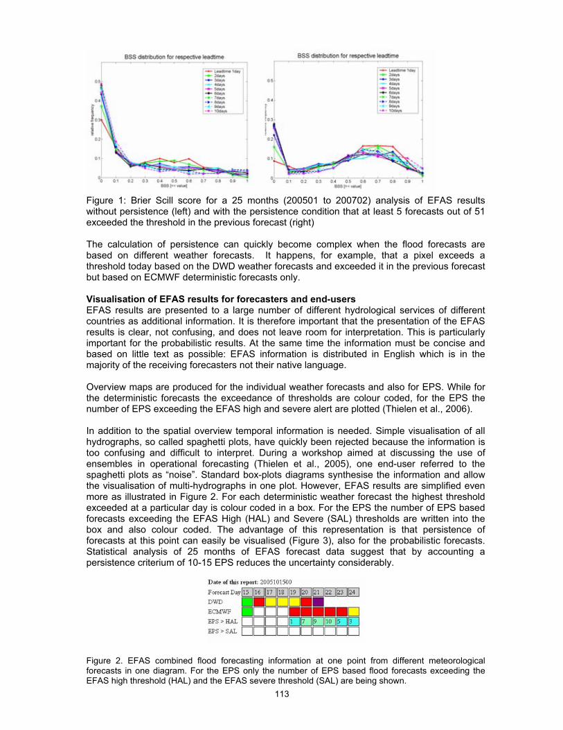
113

Figure 1: Brier Scill score for a 25 months (200501 to 200702) analysis of EFAS results without persistence (left) and with the persistence condition that at least 5 forecasts out of 51 exceeded the threshold in the previous forecast (right) The calculation of persistence can quickly become complex when the flood forecasts are based on different weather forecasts. It happens, for example, that a pixel exceeds a threshold today based on the DWD weather forecasts and exceeded it in the previous forecast but based on ECMWF deterministic forecasts only. Visualisation of EFAS results for forecasters and end-users EFAS results are presented to a large number of different hydrological services of different countries as additional information. It is therefore important that the presentation of the EFAS results is clear, not confusing, and does not leave room for interpretation. This is particularly important for the probabilistic results. At the same time the information must be concise and based on little text as possible: EFAS information is distributed in English which is in the majority of the receiving forecasters not their native language. Overview maps are produced for the individual weather forecasts and also for EPS. While for the deterministic forecasts the exceedance of thresholds are colour coded, for the EPS the number of EPS exceeding the EFAS high and severe alert are plotted (Thielen et al., 2006). In addition to the spatial overview temporal information is needed. Simple visualisation of all hydrographs, so called spaghetti plots, have quickly been rejected because the information is too confusing and difficult to interpret. During a workshop aimed at discussing the use of ensembles in operational forecasting (Thielen et al., 2005), one end-user referred to the spaghetti plots as “noise”. Standard box-plots diagrams synthesise the information and allow the visualisation of multi-hydrographs in one plot. However, EFAS results are simplified even more as illustrated in Figure 2. For each deterministic weather forecast the highest threshold exceeded at a particular day is colour coded in a box. For the EPS the number of EPS based forecasts exceeding the EFAS High (HAL) and Severe (SAL) thresholds are written into the box and also colour coded. The advantage of this representation is that persistence of forecasts at this point can easily be visualised (Figure 3), also for the probabilistic forecasts. Statistical analysis of 25 months of EFAS forecast data suggest that by accounting a persistence criterium of 10-15 EPS reduces the uncertainty considerably.

Figure 2. EFAS combined flood forecasting information at one point from different meteorological forecasts in one diagram. For the EPS only the number of EPS based flood forecasts exceeding the EFAS high threshold (HAL) and the EFAS severe threshold (SAL) are being shown.

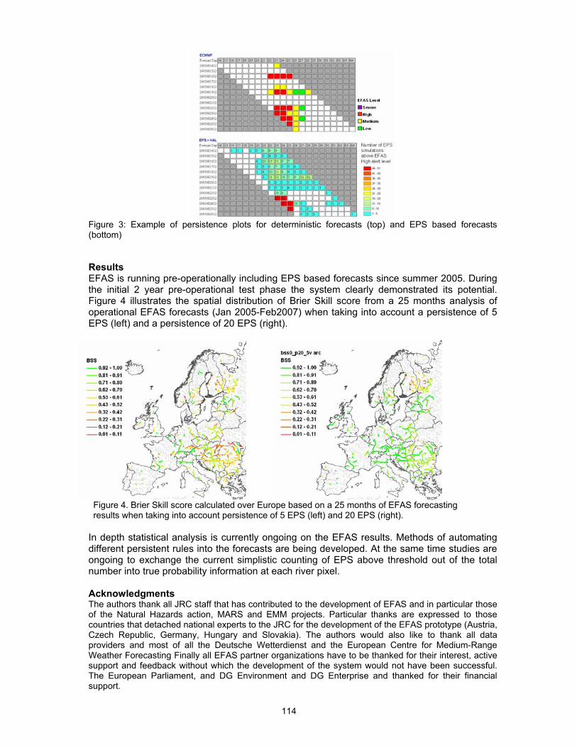
114

Figure 3: Example of persistence plots for deterministic forecasts (top) and EPS based forecasts (bottom) Results EFAS is running pre-operationally including EPS based forecasts since summer 2005. During the initial 2 year pre-operational test phase the system clearly demonstrated its potential. Figure 4 illustrates the spatial distribution of Brier Skill score from a 25 months analysis of operational EFAS forecasts (Jan 2005-Feb2007) when taking into account a persistence of 5 EPS (left) and a persistence of 20 EPS (right).

Figure 4. Brier Skill score calculated over Europe based on a 25 months of EFAS forecasting results when taking into account persistence of 5 EPS (left) and 20 EPS (right).

In depth statistical analysis is currently ongoing on the EFAS results. Methods of automating different persistent rules into the forecasts are being developed. At the same time studies are ongoing to exchange the current simplistic counting of EPS above threshold out of the total number into true probability information at each river pixel. Acknowledgments The authors thank all JRC staff that has contributed to the development of EFAS and in particular those of the Natural Hazards action, MARS and EMM projects. Particular thanks are expressed to those countries that detached national experts to the JRC for the development of the EFAS prototype (Austria, Czech Republic, Germany, Hungary and Slovakia). The authors would also like to thank all data providers and most of all the Deutsche Wetterdienst and the European Centre for Medium-Range Weather Forecasting Finally all EFAS partner organizations have to be thanked for their interest, active support and feedback without which the development of the system would not have been successful. The European Parliament, and DG Environment and DG Enterprise and thanked for their financial support.

115

References - De Roo, A., Wesseling, C. G. & Van Deurssen, W. P. A. (2000). Physically based river basin modelling within a GIS: the LISFLOOD model. Hydrological Processes, Vol. 4, Issues 11-12, p.1981-1992. - EEA, European Environment Agency (2003). Mapping the impacts of recent natural disasters and technological accidents in Europe. Environmental issue report No 35, published by European Environment Agency, Copenhagen, 2003, 47p.. - Gouweleeuw, B., Thielen, J., Franchello, G., De Roo, A., Buizza, R. (2005). Flood forecasting using medium-range probabilistic weather prediction. Hydrological and Earth System Sciences, 9(4), p.365-380. - Kowalski-Trakofler., K.M., Vaught, C., and Scharf T., (2003) Judgement and decision making under stress: an overview for emergency managers; Int. J. Emergeny Management, Vol. 1., No. 3., pp. 278-289 - Paton D., and Flin R. (1999) Disaster Stress: an emergency management perspective; Disaster Prevention and Management, Vol. 8, Nr. 4, pp 261-267 - Thielen, J., Bartholmes, J., Ramos, M-H., Kalas, M., van der Knijff, J. & De Roo, A. (2006). Added value of ensemble prediction system products for medium-range flood forecasting on European scale. In: Proceedings of the workshop “Ensemble Predictions and Uncertainties in Flood Forecasting”, International Commission for the Hydrology of the Rhine Basin (CHR), Bern Switzerland, 30-31 March 2006, p.77-82. - Thielen J, Ramos, M.H., Bartholmes, J., De Roo, A., Cloke, H., Pappenberger, F., Demeritt, D. (2005). Summary report of the 1st EFAS workshop on the use of Ensemble Prediction System in flood forecasting, 21-22nd November 2005, Ispra. European Report EUR 22118 EN, European Commissions 2005, 23p. - Van Der Knijff, J. & A. De Roo (2006). LISFLOOD – distributed water balance and flood simulation model. User manual; EUR Report EUR 22166 EN

116

Reconciling hydrological physically based models and data driven models in terms of predictive probability by E. Todini, G. Coccia and C. Mazzetti

Reconciling Hydrological Physically Based Models and Data Driven Models in Terms of Predictive Probability E. Todini, G. Coccia, C. Mazzetti University of Bologna, Italy E-mail: todini@geomin.unibo.it, gabriele.coccia@gmail.com, mazzetti@geomin.unibo.it For many years, hydrologists have debated the appropriateness of using data driven models as opposed to physically based models for flood forecasting and, in particular, for real time flood forecasting. More recently, several tentative have been made for combining the forecasts given by different types of models, by means of Bayesian weighting (Raftery et al., 2003; 2005). In this paper a new approach is presented that combines the different models in terms of the conditional predictive probability. Following the work of Krzysztofowicz (1999), by taking advantage of the Normal Quantile Transform (Van der Waerden, 1952; 1953a; 1953b; Kelly and Krzysztofowicz, 1997), one can transform the observations, namely the predictand y , as well as each of the n model

predictions n,...1iyi = into a Normal space where one obtains the images of the

observations and the models predictions, respectively denoted as η and n,...1iˆ i =η . The joint distribution of these variables can be assumed approximately normal. From the joint distribution it is then possible to derive the conditional distribution ( )n,...1iˆ itt =ηηϕ using the property of the multivariate Normal distribution. The

conditional distribution is a Normal distribution and it is easy to calculate his mean and his variance only by estimating the correlation coefficients ρ among the different vectors, namely

,.......,.......,,,.......,,,323121321 ˆ,ˆˆ,ˆˆ,ˆˆ,ˆ,ˆ, yyyyyyyyyyyy ρρρρρρ .

The following step is to obtain the conditional distribution in the real world, namely predictive probability ( )nyyyyf ˆ,...,ˆ,ˆ 21 ; this distribution represents the probability of observing the predictand given the different model output. Knowing the conditional distribution it is possible calculate the conditional expected value and its variance. This approach differs from the Bayesian processor proposed by Krzysztofowicz (1999), which implies the independence of the data driven model forecast (in that case a lag-one auto-regressive model) from the physically based model forecast. As a matter of fact, although the different model forecasts are issued independently, they cannot be statistically independent, given that they all aim at representing the same quantity, the predictand, with which they inevitably are correlated. The approach was tested in two cases. The first one, a real time flood forecasting problem on the Po river in Italy, is based on the combination of a physically based flood routing model (PAB – Todini and Bossi, 1986) and a Nearest Neighbour approach (Yakowitz, 1987; Yakowitz and Karlsson 1987, Todini, 1999). The second one is a real time flood forecasting for the Parma river based on the combination of a physically based hydrological model, the TOPKAPI, (Todini, 1995; Todini and Ciarapica, 2002; Liu and Todini, 2002), and a Data Driven Model, namely an Artificial Neural Network model (Corani and Guariso, 2002; Garcia-Bartual, 2002; Hsu et al., 1993). In both cases the results have underlined the obtainable improvements with respect to the Krzysztofowicz (1999) approach. This is quite evident in the case of the 36 hours in advance forecast for the Po river at Pontelagoscuro. Not only the bias is fully eliminated (Fig. 1) but the predictive uncertainty is further reduced (Fig. 2).

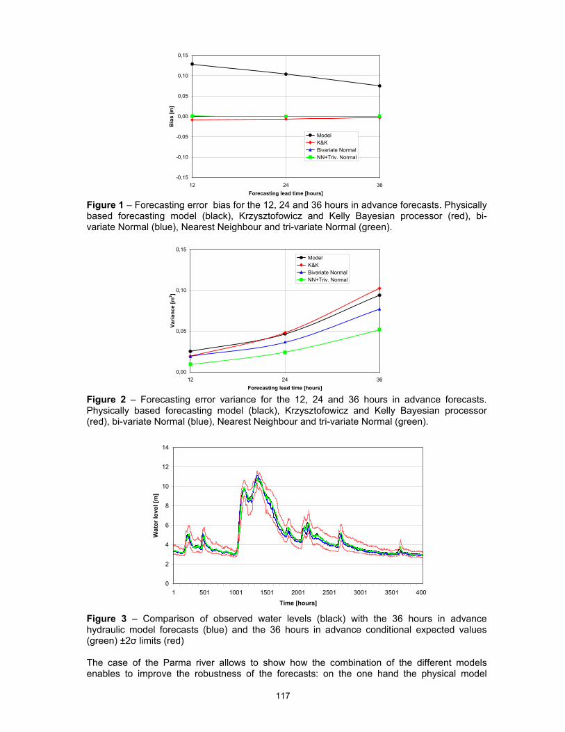
117

-0,15

-0,10

-0,05

0,00

0,05

0,10

0,15

12 24 36Forecasting lead time [hours]

Bia

s [m

]

Model K&K Bivariate Normal NN+Triv. Normal

Figure 1 – Forecasting error bias for the 12, 24 and 36 hours in advance forecasts. Physically based forecasting model (black), Krzysztofowicz and Kelly Bayesian processor (red), bi-variate Normal (blue), Nearest Neighbour and tri-variate Normal (green).

0,00

0,05

0,10

0,15

12 24 36Forecasting lead time [hours]

Varia

nce

[m2 ]

Model K&K Bivariate Normal NN+Triv. Normal

Figure 2 – Forecasting error variance for the 12, 24 and 36 hours in advance forecasts. Physically based forecasting model (black), Krzysztofowicz and Kelly Bayesian processor (red), bi-variate Normal (blue), Nearest Neighbour and tri-variate Normal (green).

0

2

4

6

8

10

12

14

1 501 1001 1501 2001 2501 3001 3501 4001

Time [hours]

Wat

er le

vel [

m]

Figure 3 – Comparison of observed water levels (black) with the 36 hours in advance hydraulic model forecasts (blue) and the 36 hours in advance conditional expected values (green) ±2σ limits (red) The case of the Parma river allows to show how the combination of the different models enables to improve the robustness of the forecasts: on the one hand the physical model

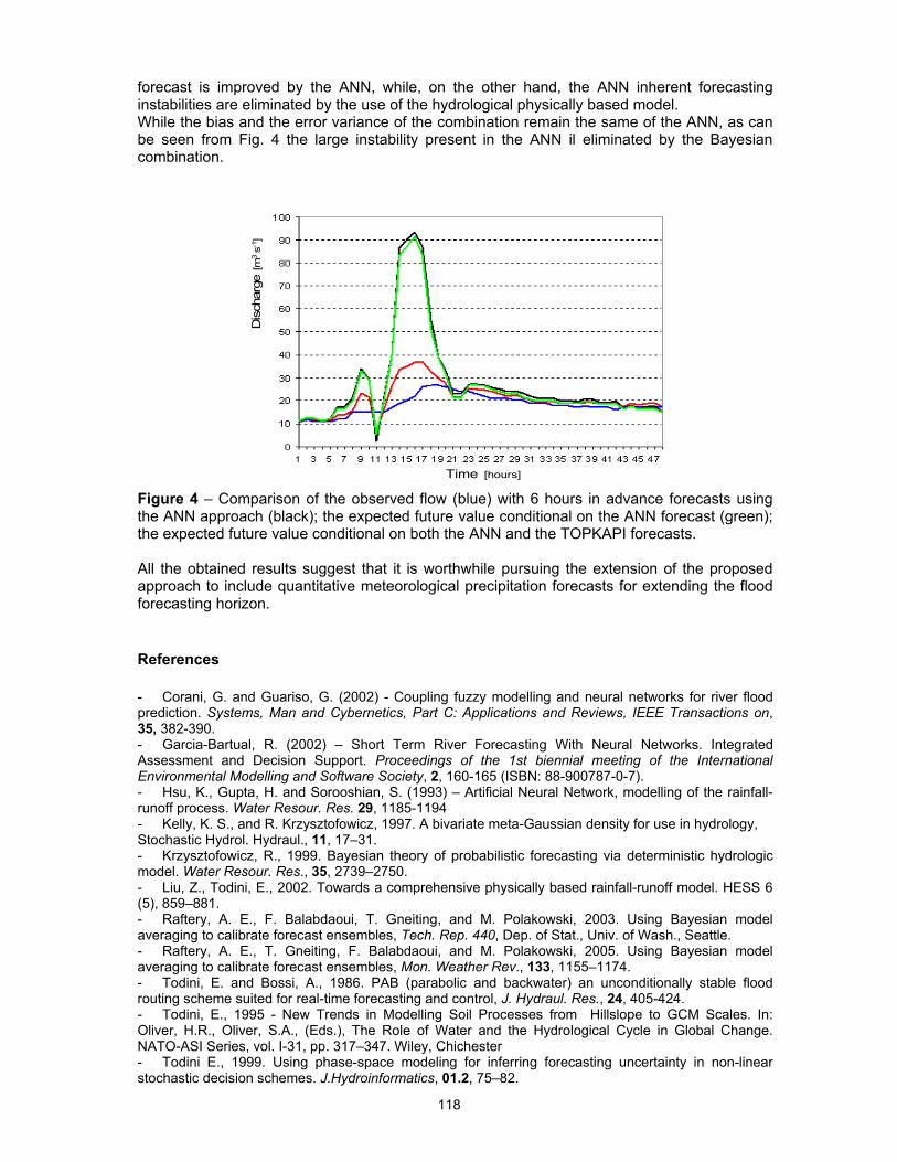
118

forecast is improved by the ANN, while, on the other hand, the ANN inherent forecasting instabilities are eliminated by the use of the hydrological physically based model. While the bias and the error variance of the combination remain the same of the ANN, as can be seen from Fig. 4 the large instability present in the ANN il eliminated by the Bayesian combination.

Time [hours]

Dis

char

ge[m

3s-

1 ]

Time [hours]

Dis

char

ge[m

3s-

1 ]

Figure 4 – Comparison of the observed flow (blue) with 6 hours in advance forecasts using the ANN approach (black); the expected future value conditional on the ANN forecast (green); the expected future value conditional on both the ANN and the TOPKAPI forecasts. All the obtained results suggest that it is worthwhile pursuing the extension of the proposed approach to include quantitative meteorological precipitation forecasts for extending the flood forecasting horizon. References - Corani, G. and Guariso, G. (2002) - Coupling fuzzy modelling and neural networks for river flood prediction. Systems, Man and Cybernetics, Part C: Applications and Reviews, IEEE Transactions on, 35, 382-390. - Garcia-Bartual, R. (2002) – Short Term River Forecasting With Neural Networks. Integrated Assessment and Decision Support. Proceedings of the 1st biennial meeting of the International Environmental Modelling and Software Society, 2, 160-165 (ISBN: 88-900787-0-7). - Hsu, K., Gupta, H. and Sorooshian, S. (1993) – Artificial Neural Network, modelling of the rainfall-runoff process. Water Resour. Res. 29, 1185-1194 - Kelly, K. S., and R. Krzysztofowicz, 1997. A bivariate meta-Gaussian density for use in hydrology, Stochastic Hydrol. Hydraul., 11, 17–31. - Krzysztofowicz, R., 1999. Bayesian theory of probabilistic forecasting via deterministic hydrologic model. Water Resour. Res., 35, 2739–2750. - Liu, Z., Todini, E., 2002. Towards a comprehensive physically based rainfall-runoff model. HESS 6 (5), 859–881. - Raftery, A. E., F. Balabdaoui, T. Gneiting, and M. Polakowski, 2003. Using Bayesian model averaging to calibrate forecast ensembles, Tech. Rep. 440, Dep. of Stat., Univ. of Wash., Seattle. - Raftery, A. E., T. Gneiting, F. Balabdaoui, and M. Polakowski, 2005. Using Bayesian model averaging to calibrate forecast ensembles, Mon. Weather Rev., 133, 1155–1174. - Todini, E. and Bossi, A., 1986. PAB (parabolic and backwater) an unconditionally stable flood routing scheme suited for real-time forecasting and control, J. Hydraul. Res., 24, 405-424. - Todini, E., 1995 - New Trends in Modelling Soil Processes from Hillslope to GCM Scales. In: Oliver, H.R., Oliver, S.A., (Eds.), The Role of Water and the Hydrological Cycle in Global Change. NATO-ASI Series, vol. I-31, pp. 317–347. Wiley, Chichester - Todini E., 1999. Using phase-space modeling for inferring forecasting uncertainty in non-linear stochastic decision schemes. J.Hydroinformatics, 01.2, 75–82.

119

- Todini, E., Ciarapica, L., 2002. The TOPKAPI model. In: Singh, V.P., Frevert, D.K., Meyer, S.P. (Eds.), Mathematical Models of Large Watershed Hydrology. Water Resources Publications, Littleton, Colorado, pp. 471–506 (Chapter 12). - Van der Waerden B.L. 1952. Order tests for two-sample problem and their power I. Indagationes Mathematicae, 14: 453-458. - Van der Waerden B.L. 1953a. Order tests for two-sample problem and their power II. Indagationes Mathematicae, 15: 303-310. - Van der Waerden B.L. 1953b. Order tests for two-sample problem and their power III. Indagationes Mathematicae, 15: 311-316. - Yakowitz S., 1987. Nearest neighbour methods for time series analysis. J. Time Ser. Anls., 8(2):235-247. - Yakowitz S. and Karlsson M., 1987. Nearest neighbour methods for time serie with application to rainfall-runoff prediction. In J.B. Mac Neil and G.H. Humphries (eds.) Stochastic Hydrology, Reidel, Hingham, Mass., pp.149-160.

120

Improving the NASA land information system in support of NOAA NWSRFS ensemble hydrologic predictions by D. Toll, B. Cosgrove, P. Houser, J. Dong and L.G. de Goncalves

IMPROVING THE NASA LAND INFORMATION SYSTEM IN SUPPORT OF NOAA NWSRFS ENSEMBLE HYDROLOGIC PREDICTIONS David Toll1*, Brian Cosgrove2, Paul Houser3, Jiarui Dong 4, and Luis Gustavo de Goncalves5 1 NASA/GSFC, Greenbelt Maryland, USA 2 NASA/GSFC/SAIC, Greenbelt Maryland, USA 3 CREW-GMU, Beltsville, Maryland, USA 4 UMBC/GEST, Catonsville, Maryland, USA 5 ORAU, Greenbelt, Maryland, USA * Corresponding author: David Toll, Code 614.3, NASA/GSFC, Greenbelt, MD USA, 301-614-5801, dave.toll@nasa.gov Abstract The NOAA National Weather Service (NWS) has 13 River Forecast Centers providing daily stream flow forecasts through their River Forecast Systems (RFS) throughout the U.S. to address a range of issues, including peak and low flow predictions as well as river floods and flash floods. Quantifying the RFS hydrologic prediction uncertainty is a primary need for NWS RFCs to identify the risk associated with the predictions and to identify areas of needed improvement. We plan to address this challenge by exploring multi-model ensemble initialization, calibration and constraint (data assimilation) within the NASA Land Information System (LIS). By enhancing LIS’s calibration and data assimilation tools for multi-model ensemble application, and including multi-model ensemble channel routing, we will enable a platform for improved NWSRFS ensemble streamflow predictions. This project partially builds on an ongoing NASA - NOAA activity integrating the NOAA Sacramento and Snow-17 models in to LIS. An end goal of this planned work is to use the LIS multi-model data assimilation and data integration capability in conjunction with NOAA Office of Hydrology Development (OHD) hydrologic prediction expertise to study ensemble hydrologic predictions for selected NOAA and HEPEX test beds. 1. Introduction A critical NOAA National Weather Service (NWS) mission is to produce forecasts for the US rivers. The NWS employs the River Forecast System (NWSRFS) at 13 River Forecast Centers (RFCs) to provide stream flow/stage forecasts on a daily to long term basis for more than 4000 points nationwide. A foremost goal of the NOAA NWS is to improve the prediction of high and low (and drought) streamflow conditions which impact water allocation for irrigation, public consumption and recreation, endangered species, and hydropower. This goal also drives the NOAA NWS Office of Hydrology (OHD), which was established to research and test activities centrally before transfer to NOAA/NWS field offices. However, there are numerous sources of variability which complicate streamflow prediction, including 1) errors in the estimation of forecast precipitation and other forcing variables, 2) uncertainties in hydrologic forecast initial conditions (e.g. dry vs. wet soils, snow pack properties, etc.), and 3) hydrologic model physics and model parameters. One of the leading approaches for reducing the uncertainties associated with hydrologic prediction is through the use of “ensemble forecasts”, where the traditional single prediction of a most likely forecast event, is replaced by an ensemble of models and forecast uncertainties (e.g., Franz et al. 2005, Buizza et al. 2005). In the ensemble approach, the production of a realistic range of initial conditions and the reduction of overall uncertainty in the resulting hydrologic predictions are both key goals (Schaake et al. 2005). This work is also towards working with the international community of researchers, water and forecast center workers to advance hydrologic forecasts through the Hydrologic Ensemble Prediction Experiment (HEPEX).

121

We plan to address this challenge by exploring multi-model ensemble initialization, calibration and constraint (data assimilation) within the Land Information System (LIS). The work described in this Abstract is towards a tentatively approved, future project to be supported by NOAA CPPA and NASA. The primary goal is to enhance the LIS calibration and data assimilation tools for multi-model ensemble application, and includes multi-model ensemble channel routing, and will enable a platform for improved NWSRFS ensemble streamflow predictions. We plan to improve hydrological forecast ensembles (< 15-days) through data assimilation of NASA satellite products and the implementation of multi-objective calibrations of hydrologic model parameters. We further plan to develop, apply and validate NASA LIS-derived ensemble hydrological predictions of up to 15 days with application and validation through collaborative work with the HEPEX Great Lakes Test Bed (PI: Vince Fortin, http://hydis8.eng.uci.edu/hepex/testbeds/GreatLakes.htm) and the emerging NOAA NWS OHD Core Project Hydrological Test Bed watersheds in the Sierra-Nevada. 2. Current Work Previous and ongoing work described below will provide the foundation for the tentatively approved project work described in this paper. Land Information System Utilized extensively in ongoing research, the recently developed, NASA Land Information System (LIS; Kumar et al., 2006) unifies and extends the capabilities of the ¼ degree Global Land Data Assimilation System (GLDAS) and the 1/8 degree North American LDAS (NLDAS) in a common software framework (see http://lis.gsfc.nasa.gov and http://ldas.gsfc.nasa.gov). It is capable of ensemble land surface modeling on points, regions or the globe at spatial resolutions from 2x2.5 degrees down to 1km. The 1km capability of LIS allows it to take advantage of the latest EOS-era observations, such as MODIS leaf area index and surface temperature, at their full resolution. The hallmark of LIS is its object-oriented software engineering design and integrated high performance computing and communications technologies that enable high-resolution ensemble land surface modeling. Examples of this design include the current LIS “plugins” for land surface models, meteorological inputs, parameters and grids/domains, which allow users to implement new functionality in any one area without affecting the rest of the code. This object-oriented design also makes LIS the ideal testbed for the development and implementation of a comprehensive model-independent, land data assimilation framework that is the subject of this work. LIS has also adopted other Earth system modeling standards and conventions, such as the Earth System Modeling Framework (ESMF) and Assistance for Land Modeling Activities (ALMA). By conforming to the standards laid out by ESMF and ALMA, LIS provides the mechanism for integrating the data assimilation framework developed in this effort with other Earth system modeling activities. These capabilities of LIS have resulted in NOAA NCEP and Air Force Weather Agency (AFWA) to incorporate LIS in to their operational framework with similar potential for NOAA OHD and RFCs. North American LDAS With strong parallels between this research and the North American LDAS project, skills gained in the NLDAS project and software used to construct the NLDAS system will be of central importance to this planned research. NLDAS provides experience in performing real-time and retrospective land surface simulations, in producing forcing data sets, in validating and intercomparing model output, and in managing data dissemination systems. NLDAS has been the basis for a wide range of domestic and international conference presentations and journal papers. In particular, 10 NLDAS articles have been published in a special issue of JGR. Including an overview (Mitchell et. al, 2004), and focusing on topics ranging from NLDAS forcing (Cosgrove et al., 2004a) to model spin-up behavior (Cosgrove et al., 2004b), these papers with others in the special journal have served as the foundation of many research projects currently underway in the land surface modeling community. NLDAS project work will provide much of the infrastructure and knowledge necessary to successfully complete the planned research. A joint project with NOAA NCEP is examining

122

the effect on NWP model forecast accuracy of initialization with offline land surface conditions. Current simulations illustrate the strong link between land surface conditions and the atmosphere, and demonstrate the positive impact that initialization of the Eta NWP model with LIS land surface conditions has on NWP forecasts of temperature, wind, and humidity. NLDAS related projects make extensive use of the LIS modeling system, which serves as a foundation for conducting the planned ensemble simulations. Evaluation of LDAS and NARR Water Budget Data for Water Resources The joint analysis of independent North American Regional Reanalysis (NARR) data, NLDAS data and in-situ measurements provides a unique look at the water and energy flux estimation from different model approaches (Dong et al. 2007, Toll et al. 2005 and Toll et al. 2006). Current US test sites include the CEOP 3-4 and Oklahoma Mesonet in the Southern Great Plains and also the Middle Rio Grande in New Mexico. Work to date has emphasized analysis of surface water and heat flux errors with analyses of approaches to reduce errors. This includes 1) correction of land cover; 2) analysis and modification of the surface albedo, 3) modification of the land surface model physics; 4) assimilation of in situ forcing to LSMs; and 5) model calibrations for the selected watersheds. NOAA-NASA NWSRFS Project Using NASA Products The planned work for this activity, builds on current work with NASA, NOAA OHD and GMU CREW to improve NOAA/NWS River Forecast Systems (NWSRFS) decision support. The overarching goal of the planned work is the demonstration of improved accuracy in runoff, flow, flood and snow monitoring and simulation from the combination of NASA satellite date and NASA LIS modeling information and infrastructure with operational NWSRFS decision support tools. The project work is currently being conducted in 3-phases. Phase 1, NASA/MSFC and NOAA/NWS/OHD researchers are using MODIS cloud cover products to improve potential evaporation estimates. Phase 2 leverages ongoing NOAA and NASA/GSFC collaboration for integration of NASA LIS and NWSRFS components and the estimation of snowpack from NASA satellite data in to the SAC/Snow-17 models. Phase 3 of the project will benchmark the Phase 1 radiation product in conjunction with the Phase 2 snow product. 3. Expected Results The primary contribution of this planned and approved project will be the development and analysis of a LIS-based system to provide ensemble hydrologic predictions (through 15 days) with a strong emphasis on streamflow predictions. However, other hydrologic forecast fields will also be available, including soil moisture, evapotranspiration and surface heat fluxes. The NASA LIS system is currently being used in a research mode by NOAA NWS NCEP with plans for an operational implementation in the near future. This LIS-based system will permit NOAA to intercompare hydrologic predictions between models under NOAA development (Noah and SAC-SMA/SNOW-17) against the performance of other land-hydrology models (USGS PRMS, NASA Catchment, and Princeton Univ. – U. Washington VIC). Also, a hypothesis for evaluation is that the five-model LIS ensemble hydrologic predictions (each forced with an ensemble of forcing data) may provide more reliable estimates than single-model ensemble forecasts. We also plan to leverage the strengths of NASA/GSFC/Hydrological Sciences Branch and GMU/CREW through further developing and evaluating the LIS Ensemble Kalman filtering tool box as applied to NASA MODIS snow cover and AMSR-E SWE and soil moisture. This data assimilation system can also be adapted for inclusion of NWSRFS in-situ point data such as streamflow and soil moisture data. Also, a significant leveraging of NASA collaborative work with Luis Bastidas (Utah State University) should result in the implementation and testing of multi-objective parameter estimate routines that will reduce uncertainties to the land-hydrology models predictions. Acknowledgements The current and planned future work is supported by the NOAA-CPPA and the NASA Terrestrial Hydrology and Applied Sciences Programs.

123

References - Buizza, R., P. Houtekamer, A. Toth, G. Pellerin, M. Wei, and Y. Zhu, 2005. A comparison of the

ECMWF, MSC, and NCEP Global Ensemble Prediction Systems, Monthly Weather Review, 133, 1076-1097.

- Cosgrove, B. A., and others, 2004a. Real-time and retrospective forcing in the North American Land Data Assimilation System (NLDAS) Project. J. Geophys. Res., 108(D22), 8842, doi:10.1029/2002JD003118, 2003.

- Cosgrove, B. A., and others, 2004b. Land surface model spin-up behavior in the North American Land Data Assimilation System (NLDAS), J. Geophys. Res., 108(D22), 8845, doi:10.1029/2002JD003316, 2003.

- Dong, J., D. L. Toll, P. R. Houser, C. Peter-Lidard, K. R. Arsenault, B. A. Cosgrove, and S. Kumar 2006a. Evaluation of the factors and error propagation in the model energy flux estimates with Land Information System, Internal review.

- Franz, K., N. Ajami, J. Schaake, and R. Buizza, 2005. Hydrologic Ensemble Experiment Focuses on Reliable Forecasts, EOS, Vol. 86 (25), 239. Section News.

- Kumar, S. V., C. D. Peters-Lidard, Y. Tian, J. Geiger, P. R. Houser, S. Olden, L. Lighty, J. L. Eastman, P. Dirmeyer, B. Doty, J. Adams, E. Wood and J. Sheffield, 2006. LIS—An interoperable framework for high resolution land surface modeling. Environmental Modeling and Software, in press, (available on-line at http://lis.gsfc.nasa.gov).

- Mitchell, K., and 21 coauthors. 2004. The multi-institution North American Land Data Assimilation System (NLDAS): Utilizing multiple GCIP products and partners in a continental distributed hydrological modeling system. J. Geophys. Res., 109: D07S90.

- Schaake, J., P. Restrepo, D. Seo, J. Demargne, L. Wu, and S. Perica, 2005. Hydrologic Ensemble Prediction: Challenges and Opportunities, International Conference on Innovative Advances and Implementation of Flood Forecasting Technology, (October),Tromso, Norway.

- Toll, D., K. Arsenault, A. Pinheiro, P. Houser, B. Cosgrove, and J. Basara, 2005. Evaluation of Land Surface Soil Moisture and Evapotranspiration using Land Data Assimilation and Information Systems for Water Resources Applications, 5th International Scientific Conference on the Global Water and Energy Cycle, (June), Costa Mesa, CA, Technical Presentation.

- Toll, D., J. Dong, P. Houser, K. Arsenault and B. Cosgrove, 2006. Land Surface Water and Energy Flux Evaluation from the North American Regional Reanalysis (NARR) and Land Data Assimilation Systems (LDAS) for Water Resources Applications, American Geophysical Union (May), Spring Meeting, Baltimore, MD, May, Poster Presentation.

124

Short- and Long-term flow forecasting in Rio Grande Water shed by C.E.M. Tucci, W. Collischonn, R.T. Clarke, A. R. Paz and D. Allasia

SHORT- AND LONG-TERM FLOW FORECASTING IN RIO GRANDE WATERSHED Carlos E. M. Tucci*, Walter Collischonn, Robin T. Clarke, Adriano R. Paz, Daniel Allasia Instituto de Pesquisas Hidráulicas, Universidade Federal do Rio Grande do Sul, Porto Alegre, Brazil. *Corresponding author: Av. Bento Gonçalves, 9500, UFRGS-IPH. 91501-970, Porto Alegre (RS), Brazil. +55 51 3308 6408; tucci@iph.ufrgs.br. Abstract As part of a research project aimed to improve short- and long-term flow forecasts used in the operational planning of Brazilian hydroelectric power systems, a large-scale distributed hydrological model has been used in combination with observed and predicted precipitation data. This paper summarizes some results obtained at Rio Grande Watershed (145 000 km2), one of the HEPEX test beds. Quantitative precipitation forecasts were provided by regional ETA model and by CPTEC global model, respectively, for short- and long-term forecasts. In the latter, a 9-member ensemble forecast was used. For short-term (time horizon up to 12 days), quality of flow forecasts obtained shows that this methodology could clearly improve operational planning of the hydroelectric reservoirs of Rio Grande watershed. Meanwhile, long-term flow forecasts (time horizon up to 6 months) were satisfactory but still require improvement on the climate forecast. 1. Introduction In Brazil, hydropower accounts for up to 83% of the total electrical energy production (ANEEL, 2005). An interconnected national transmission network allows the integrated management of the energy produced in hydroelectric dams and others sources by the national system operator (ONS). The decision making process is achieved taking into account the use of optimization models which are strongly dependent on the forecast of energy load and water availability. Currently, flow forecasts are determined using stochastic models based on precipitation and streamflow time series. As part of a research project aimed to improve short- and long-term flow forecasts used in the operational planning of Brazilian hydroelectric power systems, a large-scale distributed hydrological model has been used in combination with observed and predicted precipitation data. This paper summarizes results obtained for short- and long-term flow forecasting in Rio Grande watershed, one of the test beds of the Hydrologic Ensemble Prediction Experiment (HEPEX). For short-term flow forecasts, observed streamflow data up to the time of forecast issue were used to update state variables calculated by the model, using an empirical data assimilation procedure. Quantitative precipitation forecasts (QPF) for 10 days in advance are used, provided by the regional ETA model from the Brazilian Center for Weather Prediction (CPTEC). For long-term flow forecasts, QPF were produced by CPTEC using the AGCM global atmospheric model (Cavalcanti et al., 2002; Marengo et al., 2005), for up to 6 months in advance. An ensemble of 9 flow forecasts was obtained based on the ensemble of precipitation forecasts. 2. Methodology 2.1 Rio Grande watershed The Rio Grande is the main tributary of the River Paraná in its upper basin (Fig. 1), drains an area of about 145000 km2 and is used extensively for hydropower generation. In total, the Rio Grande watershed has an installed capacity of about 7722 MW, which corresponds to approximately 11.7% of the Brazilian total (ANEEL, 2005).

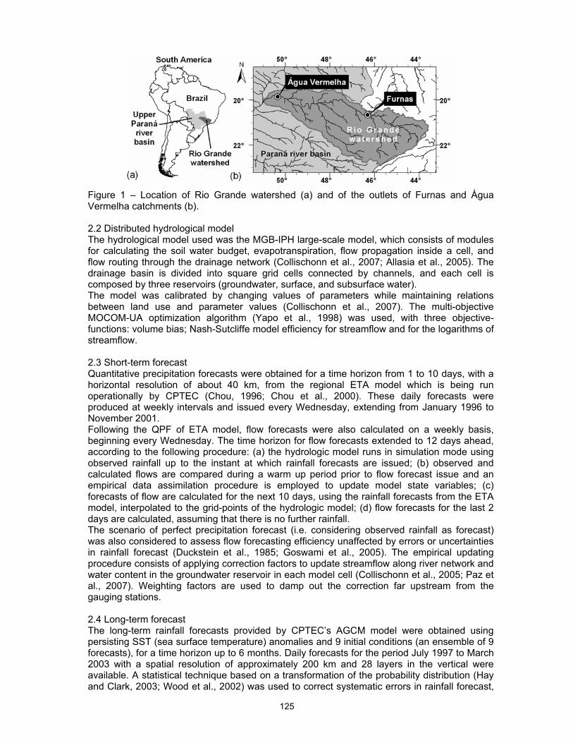
125

Figure 1 – Location of Rio Grande watershed (a) and of the outlets of Furnas and Água Vermelha catchments (b). 2.2 Distributed hydrological model The hydrological model used was the MGB-IPH large-scale model, which consists of modules for calculating the soil water budget, evapotranspiration, flow propagation inside a cell, and flow routing through the drainage network (Collischonn et al., 2007; Allasia et al., 2005). The drainage basin is divided into square grid cells connected by channels, and each cell is composed by three reservoirs (groundwater, surface, and subsurface water). The model was calibrated by changing values of parameters while maintaining relations between land use and parameter values (Collischonn et al., 2007). The multi-objective MOCOM-UA optimization algorithm (Yapo et al., 1998) was used, with three objective-functions: volume bias; Nash-Sutcliffe model efficiency for streamflow and for the logarithms of streamflow. 2.3 Short-term forecast Quantitative precipitation forecasts were obtained for a time horizon from 1 to 10 days, with a horizontal resolution of about 40 km, from the regional ETA model which is being run operationally by CPTEC (Chou, 1996; Chou et al., 2000). These daily forecasts were produced at weekly intervals and issued every Wednesday, extending from January 1996 to November 2001. Following the QPF of ETA model, flow forecasts were also calculated on a weekly basis, beginning every Wednesday. The time horizon for flow forecasts extended to 12 days ahead, according to the following procedure: (a) the hydrologic model runs in simulation mode using observed rainfall up to the instant at which rainfall forecasts are issued; (b) observed and calculated flows are compared during a warm up period prior to flow forecast issue and an empirical data assimilation procedure is employed to update model state variables; (c) forecasts of flow are calculated for the next 10 days, using the rainfall forecasts from the ETA model, interpolated to the grid-points of the hydrologic model; (d) flow forecasts for the last 2 days are calculated, assuming that there is no further rainfall. The scenario of perfect precipitation forecast (i.e. considering observed rainfall as forecast) was also considered to assess flow forecasting efficiency unaffected by errors or uncertainties in rainfall forecast (Duckstein et al., 1985; Goswami et al., 2005). The empirical updating procedure consists of applying correction factors to update streamflow along river network and water content in the groundwater reservoir in each model cell (Collischonn et al., 2005; Paz et al., 2007). Weighting factors are used to damp out the correction far upstream from the gauging stations. 2.4 Long-term forecast The long-term rainfall forecasts provided by CPTEC’s AGCM model were obtained using persisting SST (sea surface temperature) anomalies and 9 initial conditions (an ensemble of 9 forecasts), for a time horizon up to 6 months. Daily forecasts for the period July 1997 to March 2003 with a spatial resolution of approximately 200 km and 28 layers in the vertical were available. A statistical technique based on a transformation of the probability distribution (Hay and Clark, 2003; Wood et al., 2002) was used to correct systematic errors in rainfall forecast,

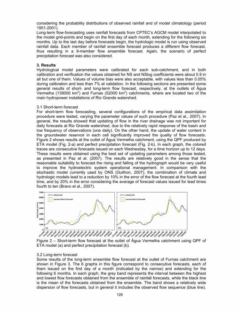
126

considering the probability distributions of observed rainfall and of model climatology (period 1951-2001). Long-term flow-forecasting uses rainfall forecasts from CPTEC’s AGCM model interpolated to the model grid-points and begin on the first day of each month, extending for the following six months. Up to the last day before forecasts begin, the hydrologic model is run using observed rainfall data. Each member of rainfall ensemble forecast produces a different flow forecast, thus resulting in a 9-member flow ensemble forecast. Again, the scenario of perfect precipitation forecast was also considered. 3. Results Hydrological model parameters were calibrated for each sub-catchment, and in both calibration and verification the values obtained for NS and NSlog coefficients were about 0.9 in all but one of them. Values of volume bias were also acceptable, with values less than 0.05% during calibration and less than 7% at validation. In the following sections are presented some general results of short- and long-term flow forecast, respectively, at the outlets of Água Vermelha (139000 km2) and Furnas (52000 km2) catchments, where are located two of the main hydropower installations of Rio Grande watershed. 3.1 Short-term forecast For short-term flow forecasting, several configurations of the empirical data assimilation procedure were tested, varying the parameter values of such procedure (Paz et al., 2007). In general, the results showed that updating of flow in the river drainage was not important for daily forecasts at Rio Grande watershed, due to the relatively rapid response of the basin and low frequency of observations (one daily). On the other hand, the update of water content in the groundwater reservoir in each cell significantly improved the quality of flow forecasts. Figure 2 shows results at the outlet of Água Vermelha catchment, using the QPF produced by ETA model (Fig. 2-a) and perfect precipitation forecast (Fig. 2-b). In each graph, the colored traces are consecutive forecasts issued on each Wednesday, for a time horizon up to 12 days. These results were obtained using the best set of updating parameters among those tested, as presented in Paz et al. (2007). The results are relatively good in the sense that the reasonable suitability to forecast the rising and falling of the hydrograph would be very useful to improve the hydroelectric system operational management. In comparison with the stochastic model currently used by ONS (Guilhon, 2007), the combination of climate and hydrologic models lead to a reduction by 10% in the error of the flow forecast at the fourth lead time, and by 20% in the error considering the average of forecast values issued for lead times fourth to ten (Bravo et al., 2007).

Figure 2 – Short-term flow forecast at the outlet of Água Vermelha catchment using QPF of ETA model (a) and perfect precipitation forecast (b). 3.2 Long-term forecast Some results of the long-term ensemble flow forecast at the outlet of Furnas catchment are shown in Figure 3. The 6 graphs in this figure correspond to consecutive forecasts, each of them issued on the first day of a month (indicated by the narrow) and extending for the following 6 months. In each graph, the grey band represents the interval between the highest and lowest flow forecasts obtained from the ensemble of rainfall forecasts, while the black line is the mean of the forecasts obtained from the ensemble. The band shows a relatively wide dispersion of flow forecasts, but in general it includes the observed flow sequence (blue line).

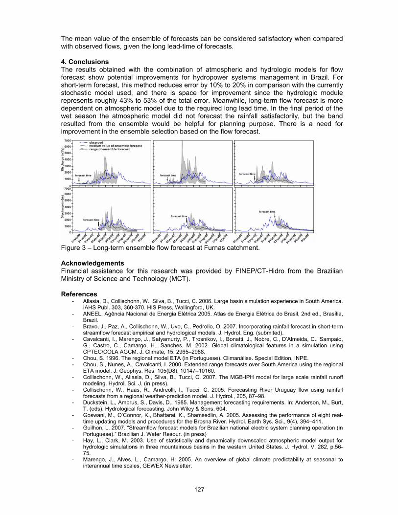
127

The mean value of the ensemble of forecasts can be considered satisfactory when compared with observed flows, given the long lead-time of forecasts. 4. Conclusions The results obtained with the combination of atmospheric and hydrologic models for flow forecast show potential improvements for hydropower systems management in Brazil. For short-term forecast, this method reduces error by 10% to 20% in comparison with the currently stochastic model used, and there is space for improvement since the hydrologic module represents roughly 43% to 53% of the total error. Meanwhile, long-term flow forecast is more dependent on atmospheric model due to the required long lead time. In the final period of the wet season the atmospheric model did not forecast the rainfall satisfactorily, but the band resulted from the ensemble would be helpful for planning purpose. There is a need for improvement in the ensemble selection based on the flow forecast.

Figure 3 – Long-term ensemble flow forecast at Furnas catchment. Acknowledgements Financial assistance for this research was provided by FINEP/CT-Hidro from the Brazilian Ministry of Science and Technology (MCT). References

- Allasia, D., Collischonn, W., Silva, B., Tucci, C. 2006. Large basin simulation experience in South America. IAHS Publ. 303, 360-370. HIS Press, Wallingford, UK.

- ANEEL, Agência Nacional de Energia Elétrica 2005. Atlas de Energia Elétrica do Brasil, 2nd ed., Brasília, Brazil.

- Bravo, J., Paz, A., Collischonn, W., Uvo, C., Pedrollo, O. 2007. Incorporating rainfall forecast in short-term streamflow forecast empirical and hydrological models. J. Hydrol. Eng. (submited).

- Cavalcanti, I., Marengo, J., Satyamurty, P., Trosnikov, I., Bonatti, J., Nobre, C., D’Almeida, C., Sampaio, G., Castro, C., Camargo, H., Sanches, M. 2002. Global climatological features in a simulation using CPTEC/COLA AGCM. J. Climate, 15: 2965–2988.

- Chou, S. 1996. The regional model ETA (in Portuguese). Climanálise. Special Edition, INPE. - Chou, S., Nunes, A., Cavalcanti, I. 2000. Extended range forecasts over South America using the regional

ETA model. J. Geophys. Res. 105(D8), 10147–10160. - Collischonn, W., Allasia, D., Silva, B., Tucci, C. 2007. The MGB-IPH model for large scale rainfall runoff

modeling. Hydrol. Sci. J. (in press). - Collischonn, W., Haas, R., Andreolli, I., Tucci, C. 2005. Forecasting River Uruguay flow using rainfall

forecasts from a regional weather-prediction model. J. Hydrol., 205, 87–98. - Duckstein, L., Ambrus, S., Davis, D., 1985. Management forecasting requirements. In: Anderson, M., Burt,

T. (eds). Hydrological forecasting. John Wiley & Sons, 604. - Goswani, M., O’Connor, K., Bhattarai, K., Shamsedlin, A. 2005. Assessing the performance of eight real-

time updating models and procedures for the Brosna River. Hydrol. Earth Sys. Sci., 9(4), 394–411. - Guilhon, L. 2007. “Streamflow forecast models for Brazilian national electric system planning operation (in

Portuguese).” Brazilian J. Water Resour. (in press) - Hay, L., Clark, M. 2003. Use of statistically and dynamically downscaled atmospheric model output for

hydrologic simulations in three mountainous basins in the western United States. J. Hydrol. V. 282, p.56-75.

- Marengo, J., Alves, L., Camargo, H. 2005. An overview of global climate predictability at seasonal to interannual time scales, GEWEX Newsletter.

128

- Paz, A., Collischonn, W., Tucci, C., Clarke, R., Allasia, D. 2007. Data assimilation in a large-scale distributed hydrological model for short range flow forecasts. IAHS Publ. 313. IAHS Press, Wallingford, UK (accepted).

- Wood, E., Maurer, E., Kumar, A., Lettenmaier, D. 2002. Long-range experimental hydrologic forecasting for the eastern United States. J. Geophys. Res. V.107, n.20, p.6(1-15).

- Yapo, P., Gupta, H., Sorooshian, S. 1998. Multi-objective global optimization for hydrologic models. J. of Hydrol., 204, 83–97.

129

U-V-W

Rijnland case study: anticipatory control of a lowlying regional water system by S. J. Van Andel, A. Lobbrecht and R. Price

RIJNLAND CASE STUDY: ANTICIPATORY CONTROL OF A LOW-LYING REGIONAL WATER SYSTEM Schalk Jan van Andel 1*, Arnold Lobbrecht1,2 and Roland Price1 1 UNESCO-IHE, Hydroinformatics and Knowledge Management, Delft, The Netherlands 2 HydroLogic, Amersfoort, The Netherlands * Corresponding author: P.O. Box 3015, 2601 DA Delft, The Netherlands, +31(0)152151803, s.vanandel@unesco-ihe.org Abstract This research focuses on the flooding problems that can occur in low-lying controlled water systems. A methodology is described in which flood control strategies based on ECMWF ensemble precipitation forecasts and hydrological models are developed using simulation and verification analysis. The methodology is applied to the Rijnland water system in the Netherlands. A control strategy for lowering the water levels in a channelled storage basin in anticipation of heavy rainfall, and based on 3-day ensemble water level forecasts, is demonstrated for a period of heavy rain in October 1998. The results show that measured peaks are successfully reduced and false alarms do not occur before the precipitation event. 1. Introduction Deltaic areas often contain low-lying controlled water systems for irrigation or land reclamation. The latter are very common in the Netherlands, where these water systems are called "polders". A polder is an area below sea level, in which the water is drained by ditches and canals and discharged out of the area by pumping stations. This research focuses on the flooding problems that can occur in these systems and how water authorities in the Netherlands try to reduce the frequency of flooding and mitigate consequential damage. One way of reducing damage due to flooding is to take pro-active control actions on the basis of precipitation forecasts and hydrological predictions. This is designated here as "Anticipatory control". A case study concerns the Rijnland water system. A methodology is described in which control strategies based on ECMWF ensemble precipitation forecasts and hydrological models are developed using simulation and verification analysis. This research focuses mainly on the end user-oriented scientific question in the HEPEX project: "What is the best way for the user community to take advantage of ensemble forecasts?" 2. Rijnland Water System The Rijnland water system is situated in the western part of the Netherlands, along the North Sea coast and north of the river Rhine. The drainage area is about 100000 ha, of which 72000 ha is 3 to 4 meters below sea-level. 23000 Ha consists of dunes and horticultural lands, which drain under gravity. The water from both the dunes and the low-lying areas is drained by a 4500 ha system of inter-connected canals with an average water level of -0.62 m+NAP (Dutch reference level ~ 0.62 m below sea level). From this channelled storage basin the water is discharged to the sea and rivers by pumping stations. The Rijnland Water Board needs to control the water level in the storage basin within a 0.05 m range (Fig. 1).

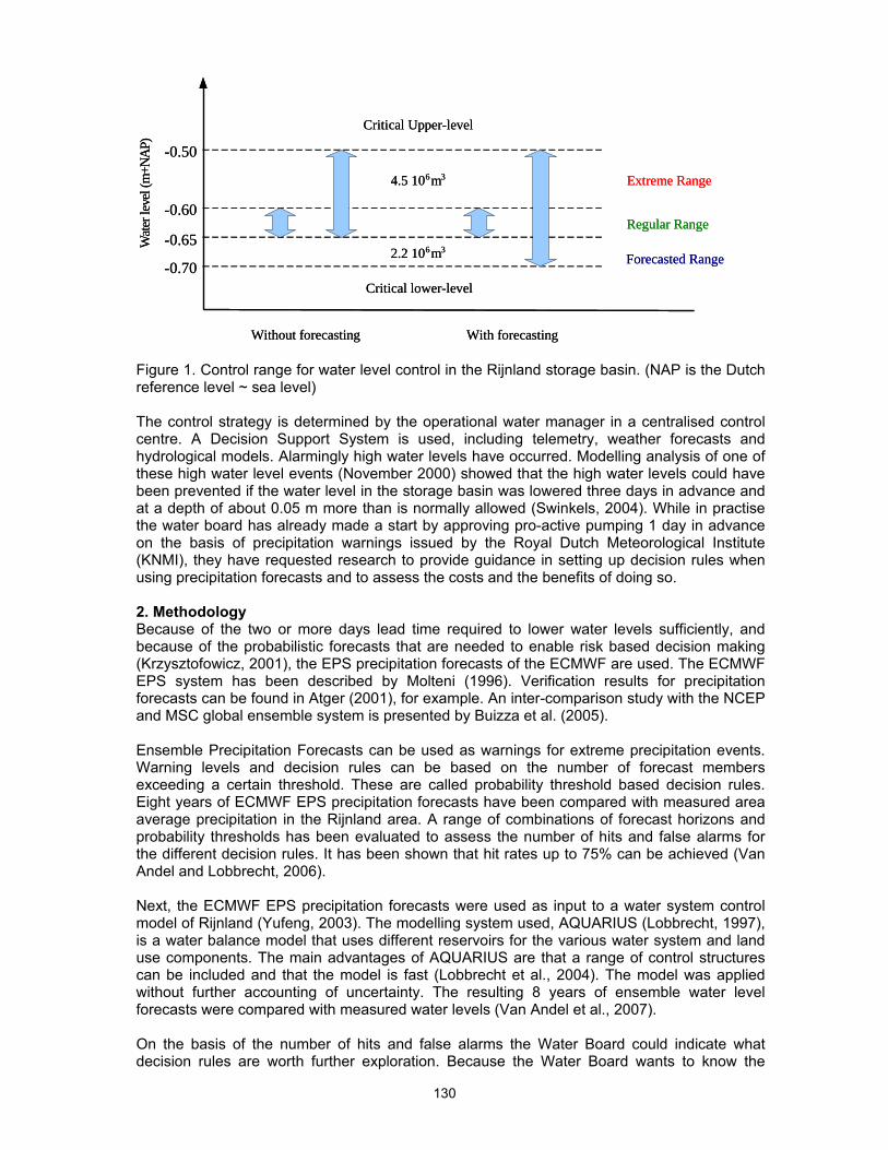
130

Wate

r lev

el(m

+NA

P) -0.50

-0.60

-0.702.2 106m3

4.5 10 6m3

Critical lower-level

Critical Upper-level

Without forecasting With forecasting

Forecasted Range

Regular Range

Extreme Range

-0.65Wate

r lev

el(m

+NA

P) -0.50

-0.60

-0.702.2 106m3

4.5 10 6m3

Critical lower-level

Critical Upper-level

Without forecasting With forecasting

Forecasted Range

Regular Range

Extreme Range

-0.65

Figure 1. Control range for water level control in the Rijnland storage basin. (NAP is the Dutch reference level ~ sea level) The control strategy is determined by the operational water manager in a centralised control centre. A Decision Support System is used, including telemetry, weather forecasts and hydrological models. Alarmingly high water levels have occurred. Modelling analysis of one of these high water level events (November 2000) showed that the high water levels could have been prevented if the water level in the storage basin was lowered three days in advance and at a depth of about 0.05 m more than is normally allowed (Swinkels, 2004). While in practise the water board has already made a start by approving pro-active pumping 1 day in advance on the basis of precipitation warnings issued by the Royal Dutch Meteorological Institute (KNMI), they have requested research to provide guidance in setting up decision rules when using precipitation forecasts and to assess the costs and the benefits of doing so. 2. Methodology Because of the two or more days lead time required to lower water levels sufficiently, and because of the probabilistic forecasts that are needed to enable risk based decision making (Krzysztofowicz, 2001), the EPS precipitation forecasts of the ECMWF are used. The ECMWF EPS system has been described by Molteni (1996). Verification results for precipitation forecasts can be found in Atger (2001), for example. An inter-comparison study with the NCEP and MSC global ensemble system is presented by Buizza et al. (2005). Ensemble Precipitation Forecasts can be used as warnings for extreme precipitation events. Warning levels and decision rules can be based on the number of forecast members exceeding a certain threshold. These are called probability threshold based decision rules. Eight years of ECMWF EPS precipitation forecasts have been compared with measured area average precipitation in the Rijnland area. A range of combinations of forecast horizons and probability thresholds has been evaluated to assess the number of hits and false alarms for the different decision rules. It has been shown that hit rates up to 75% can be achieved (Van Andel and Lobbrecht, 2006). Next, the ECMWF EPS precipitation forecasts were used as input to a water system control model of Rijnland (Yufeng, 2003). The modelling system used, AQUARIUS (Lobbrecht, 1997), is a water balance model that uses different reservoirs for the various water system and land use components. The main advantages of AQUARIUS are that a range of control structures can be included and that the model is fast (Lobbrecht et al., 2004). The model was applied without further accounting of uncertainty. The resulting 8 years of ensemble water level forecasts were compared with measured water levels (Van Andel et al., 2007). On the basis of the number of hits and false alarms the Water Board could indicate what decision rules are worth further exploration. Because the Water Board wants to know the

131

highest achievable level of safety against flooding, they are interested in looking at the highest forecast for the three day forecast horizon, including the previous forecasts for that event (t-1day, t-2days, etc.). The anticipatory control strategy was chosen such that if one of the forecasts for the three day horizon exceeds -0.57 m+NAP, the level in the storage basin is drawn down to between -0.65 and -0.70 m+NAP in order to create extra storage at the beginning of the precipitation event. 3. Results The effect of this control strategy was simulated using the combined ECMWF EPS precipitation forecasts and the AQUARIUS water system control model for a period of heavy precipitation in October 1998. One of the ensemble forecasts is shown in Figure 2. It can be seen that several members exceed the -0.57 m+NAP level for several days. Therefore the model will activate the pumping stations and draw down the water level. The results are presented in Figure 3. The thin line presents the historically measured water level in the storage basin. The extreme low levels represent missing data. It can be seen that between October 25 and November 6, peaks above -0.60 m+NAP occurred. The thick line presents the simulated water level with anticipatory lowering of water levels to -0.70 m+NAP on the basis of the EPS water level forecasts. It can be seen that the extra storage prevents the water level from exceeding -0.60 m+NAP. In the period between 10 and 23 October the modelled and measured water levels are about the same. This shows that for this period no false alarms occurred and no unnecessary lowering of the water level in the storage basin was performed. 5. Conclusion A methodology has been developed to simulate and evaluate anticipatory water system control on the basis of ensemble precipitation forecasts and water level predictions. The methodology is applied to a case study in the Netherlands of a low-lying controlled channelled storage basin. A control strategy that prescribes the lowering of the water level in the storage basin in anticipation of a heavy rainfall event based on 3-day ensemble water level forecasts, is demonstrated for an event in October 1998. The results show that measured peaks would have been successfully reduced using the anticipatory control strategy. This research provides insight into the opportunities and challenges for using hydrological ensemble predictions in operational water management. The results show that the current global EPS systems already have great potential for regional water system control. The methods used can also be applied to river flood forecasting and early warning and reservoir control.

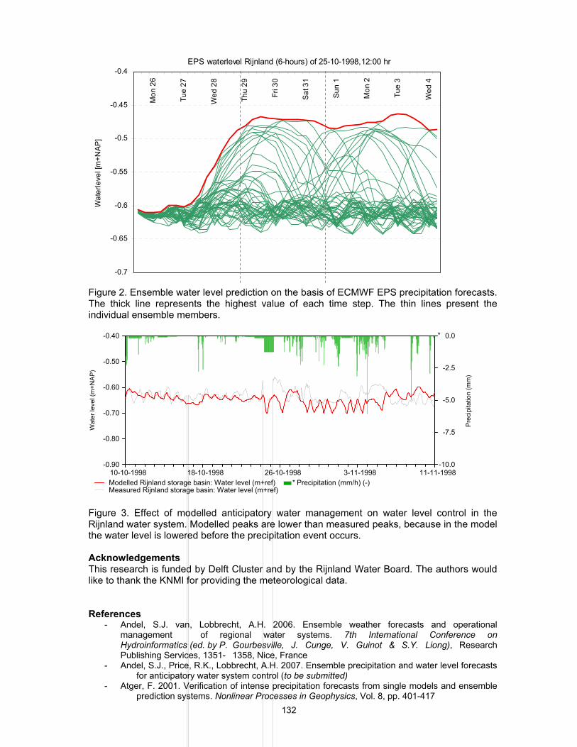
132

-0.7

-0.65

-0.6

-0.55

-0.5

-0.45

-0.4

Mon

26

Tue

27

Wed

28

Thu

29

Fri 3

0

Sat

31

Sun

1

Mon

2

Tue

3

Wed

4

Wat

erle

vel [

m+N

AP

]

EPS waterlevel Rijnland (6-hours) of 25-10-1998,12:00 hr

Figure 2. Ensemble water level prediction on the basis of ECMWF EPS precipitation forecasts. The thick line represents the highest value of each time step. The thin lines present the individual ensemble members.

*

-0.90

-0.80

-0.70

-0.60

-0.50

-0.40

Wat

er le

vel (

m+N

AP

)

-10.0

-7.5

-5.0

-2.5

0.0

Pre

cipi

tatio

n (m

m)

Modelled Rijnland storage basin: Water level (m+ref) * Precipitation (mm/h) (-)Measured Rijnland storage basin: Water level (m+ref)

10-10-1998 18-10-1998 26-10-1998 3-11-1998 11-11-1998

Figure 3. Effect of modelled anticipatory water management on water level control in the Rijnland water system. Modelled peaks are lower than measured peaks, because in the model the water level is lowered before the precipitation event occurs. Acknowledgements This research is funded by Delft Cluster and by the Rijnland Water Board. The authors would like to thank the KNMI for providing the meteorological data. References

- Andel, S.J. van, Lobbrecht, A.H. 2006. Ensemble weather forecasts and operational management of regional water systems. 7th International Conference on Hydroinformatics (ed. by P. Gourbesville, J. Cunge, V. Guinot & S.Y. Liong), Research Publishing Services, 1351- 1358, Nice, France

- Andel, S.J., Price, R.K., Lobbrecht, A.H. 2007. Ensemble precipitation and water level forecasts for anticipatory water system control (to be submitted)

- Atger, F. 2001. Verification of intense precipitation forecasts from single models and ensemble prediction systems. Nonlinear Processes in Geophysics, Vol. 8, pp. 401-417

133

- Buizza, R., Houtekamer, P.L., Toth, Z., Pellerin, G., Wei, M., Zhu, Y. 2005. Comparison of the ECMWF, MSC, and NCEP Global Ensemble Prediction Systems. Monthly Weather Review, Vol. 133, pp. 1076-1097

- Krzysztofowicz, R. 2001. The case for probabilistic forecasting in hydrology. Journal of Hydrology 249, pp.2-9.

- Lobbrecht, A. H. 1997. Dynamic Water-System Control, Design and Operation of Regional Water-Resources Systems, Dissertation, A. A. Balkema Publishers, ISBN 9054104325

- Lobbrecht, A.H., Dibike, Y., Solomatine, D.P. 2004. Artificial Neural Networks and Fuzzy Systems in Model Based Control of the Overwaard Polder. ASCE Journal of Water Resources Planning and Management

- Molteni, F., Buizza, R., Palmer, T.N., Petrogliatis, T. 1996. The ECMWF Ensemble Prediction System: Methodology and validation. Quart. J. Roy. Meteor. Soc., 122, 73–119.

- Swinkels, M. A. J. 2004. Control rules for operational management of polder storage basin systems. M.Sc. Thesis, Technical University Delft (in Dutch)

- Yufeng, G. 2003. Flood Modelling and Forecasting for Rijnland Area Using Physically Based and Data-Driven Methods. M.Sc. Thesis, HH 470, UNESCO-IHE, Delft, the Netherlands

134

Downscaling global medium range meteorological predictions for flood prediction by N. Voisin, A.W. Wood and D.P. Lettenmaier

DOWNSCALING GLOBAL MEDIUM RANGE METEOROLOGICAL PREDICTIONS FOR FLOOD PREDICTION Voisin, N. 1, A.W. Wood 1 and D.P. Lettenmaier 1* 1 Civil and Environmental Engineering, University of Washington * Corresponding author: Dennis Letttenmaier, Civil and Environmental Engineering, University of Washington, Hydrology Group, P.O. Box 352700, Seattle, WA 98195-2700, USA, dennisl@u.washington.edu We describe a prototype system for medium range (up to two week lead) flood prediction in large rivers, which is intended for global implementation. The procedure draws from the experimental North American Land Data Assimilation System (NLDAS) and the companion Global Land Data Assimilation System (GLDAS) and the University of Washington West-wide Seasonal Hydrologic Forecast System for streamflow prediction. Hydrologic forecasts based on numerical weather prediction (NWP) serve both as the source of nowcasts (for hydrologic model initialization) and forecasts for lead times up to fifteen days. The use of forecast models and satellite remote sensing in this procedure reduces the need for in situ precipitation and other observations in parts of the world where surface networks are critically deficient, but where a global hydrologic forecast capability arguably would have the greatest value. The hydrologic component of the system is the Variable Infiltration Capacity (VIC) macroscale hydrology model. In the prototype, VIC is spun up for forecast initialization using daily ERA-40 precipitation, ERA-40 wind, and ERA-40 surface air temperature. In hindcast mode, VIC is driven by global NCEP ensemble 15-day re-forecasts (NOAA/ESRL) that are bias corrected with respect to ERA-40 data and spatially disaggregated using two higher spatial resolution satellite products: Global Precipitation Climatology Project (GPCP) 1dd daily precipitation and Tropical Rainfall Measuring System (TRMM) 3B42 precipitation. The prototype system is implemented globally at one-half degree spatial resolution tested during the 1979-August 2002 period. To make the system operational in near-real time, the system simulation will be updated to the present time using the NCEP analysis, bias corrected with respect to the ERA40. This presentation focuses on verification of forecast error statistic predictions for the Mississippi Basin resulting from application of the entire downscaling sequence.

135

Recent advances in data assimilation and postprocessing in operational ensemble flood forecasting by A. Weerts, P. Reggiani and M. Werner

Recent advances in data assimilation and postprocessing in operational ensemble flood forecasting Albrecht Weerts, Paolo Reggiani, Micha Werner WL | Delft Hydraulics P.O. Box 177, 2600MH Delft, The Netherlands The poster presents an overview of research activities that have and will be carried out at WL|Delft Hydraulics in the context of operational flood forecasting. Firstly a data assimilation (DATools) and an uncertainty analysis tool kit (UATools) have been developed. These instruments can be either used in stand-alone mode or can be embedded in the form of a specific module into the generic flood forecasting environment Delft-FEWS for assimilating operationally observations into hydraulic and hydrological models via Ensemble Kalman Filtering (EnKF) or Particle Filtering techniques. Secondly, research activities in post-processing of precipitation (HIRLAM weather model) and discharge forecast for the river Rhine using Bayesian revision of prior probability distributions on forecasted flow have been carried out. So far, these methods have been tested preliminarily using deterministic precipitation forecasts. The methodology can be extended to a Bayesian ensemble forecasting by including ensemble precipitation forecasts. Thirdly, research into Bayesian model averaging (BMA) for operational forecasting of storm surges in the North Sea using the North-West Shelf Operational Oceanic System (NOOS) has recently been started. This post-processing technique can readily be applied to flood forecasting. A brief indication is given on how this extension to Bayesian model averaging can be implemented in this context.

136

Multiple ensemble forecasts in the operational forecasting system for the Rhine basin in Switzerland by M. Werner, M.v.Dijk, T. Buergli and S. Vogt

Multiple ensemble forecasts in the operational forecasting system for the Rhine basin in Switzerland Micha Werner, Marc van Dijk WL | Delft Hydraulics P.O. Box 177, 2600MH Delft, The Netherlands Therese Bürgi, Stephan Vogt Federal Office for the Environment FOEN 3003 Bern-Ittigen, Switzerland With the advent of meteorological ensemble forecasting, ensemble approaches in operational flood forecasting are now also becoming more and more prolific. Where uncertainty in the hydrological forecast has previously either been ignored or has been incorporated through empirical approaches, the more statistically sound approach to representation of uncertainty through ensemble based forecasts are being adopted. The operational forecasting system for Rhine basin in Switzerland, which is used operationally by the Swiss Federal Office for the Environment currently uses such an empirical approach to representing uncertainty. Within the context of the WMO sponsored MAP-D Phase project, ensemble forecasts are now being integrated into the operational forecasts to provide for the representation of uncertainty. This considers multiple ensembles, including the high resolution COSMO-LEPS ensemble and the multi-model SRNWP-PEPS ensemble. The ECMWF-EPS ensemble was not considered for operational use, but has been included for comparison to the high resolution ensembles. In this poster some initial results from the integration of these ensembles into the operational forecasting system are presented. Although the usage and evaluation of these ensembles are as yet in the early stages, initial results show that several scientifically challenging questions on the use of ensemble forecasting in hydrology are yet to be resolved. These include the spatial and temporal scale issues of the different ensembles, as well as issues in dealing with multiple and multi-model ensembles in decision making.

137

Correcting errors in streamflow forecast ensemble mean and spread by A. Wood Correcting errors in streamflow forecast ensemble mean and spread Andrew Wood Department of Civil and Environmental Engineering, University of Washington, Seattle, WA 98115 When hydrological models are used for probabilistic streamflow forecasting in the Ensemble Streamflow Prediction (ESP) framework, the deterministic simulation used for initialization can lead to the underestimation of forecast uncertainty, as represented by the spread of the forecast ensemble. One avenue for correcting the resulting forecast reliability errors is to calibrate the forecast ensemble outputs to match their observed error characteristics. This paper outlines and evaluates an approach for forecast calibration, as applied to seasonal streamflow prediction. The approach uses the correlation of forecast ensemble means with observations to generate a conditional forecast mean and spread that lie between the climatological mean and spread (when no correlation exists) and the raw forecast mean and zero spread (when the correlation is perfect). Retrospective forecasts of summer period runoff for the Feather River basin, CA, are used to demonstrate that the approach reduces errors in forecast mean and spread, thereby improving the forecasts' reliability for water management uses.

138

Using CPC seasonal climate outlooks for ensemble hydrologic prediction by A. Wood, X. Zeng and D. P. Lettenmaier

Using CPC seasonal climate outlooks for ensemble hydrologic prediction Andrew Wood, Xiaodong Zeng and Dennis P. Lettenmaier Department of Civil and Environmental Engineering, University of Washington, Seattle, WA 98115 Seasonal forecasts from the Climate Prediction Center’s (CPC) new objective, consolidated temperature and precipitation prediction product are used to drive ensemble streamflow predictions for river basins in the western U.S. To create ensembles from the parametric CPC forecasts, we resample historical temperature and precipitation sequences serving as retrospective input to the hydrologic model, and adjust them to exhibit the mean anomalies of the CPC forecasts. Different approaches for constraining the spread of the climate forecast ensemble, including as a baseline the use of climatological spread, are being evaluated. This presentation outlines the procedure for using the climate forecast product to form ensembles, and summarizes results from an ongoing evaluation of the climate and hydrologic forecasts produced in this manner.

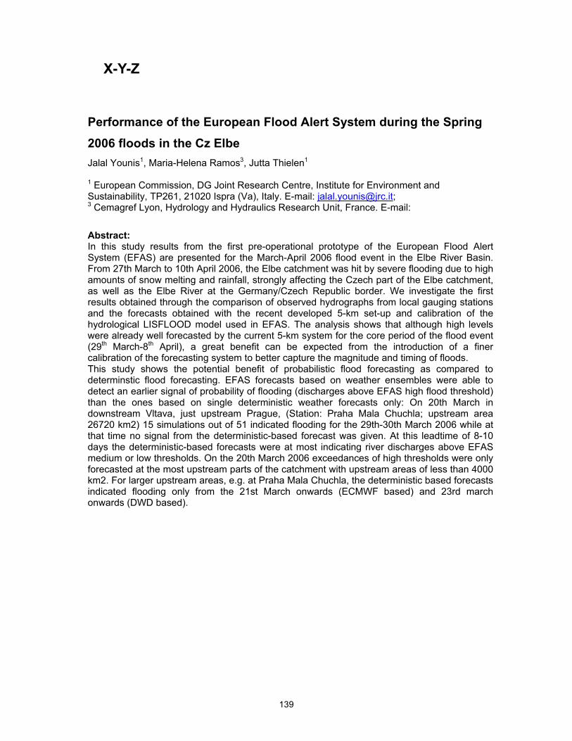
139

X-Y-Z

Performance of the European Flood Alert System during the Spring 2006 floods in the Cz Elbe by J. Younis, M.H. Ramos and J. Thielen

Performance of the European Flood Alert System during the Spring 2006 floods in the Cz Elbe Jalal Younis1, Maria-Helena Ramos3, Jutta Thielen1 1 European Commission, DG Joint Research Centre, Institute for Environment and Sustainability, TP261, 21020 Ispra (Va), Italy. E-mail: jalal.younis@jrc.it; 3 Cemagref Lyon, Hydrology and Hydraulics Research Unit, France. E-mail: Abstract: In this study results from the first pre-operational prototype of the European Flood Alert System (EFAS) are presented for the March-April 2006 flood event in the Elbe River Basin. From 27th March to 10th April 2006, the Elbe catchment was hit by severe flooding due to high amounts of snow melting and rainfall, strongly affecting the Czech part of the Elbe catchment, as well as the Elbe River at the Germany/Czech Republic border. We investigate the first results obtained through the comparison of observed hydrographs from local gauging stations and the forecasts obtained with the recent developed 5-km set-up and calibration of the hydrological LISFLOOD model used in EFAS. The analysis shows that although high levels were already well forecasted by the current 5-km system for the core period of the flood event (29th March-8th April), a great benefit can be expected from the introduction of a finer calibration of the forecasting system to better capture the magnitude and timing of floods. This study shows the potential benefit of probabilistic flood forecasting as compared to determinstic flood forecasting. EFAS forecasts based on weather ensembles were able to detect an earlier signal of probability of flooding (discharges above EFAS high flood threshold) than the ones based on single deterministic weather forecasts only: On 20th March in downstream Vltava, just upstream Prague, (Station: Praha Mala Chuchla; upstream area 26720 km2) 15 simulations out of 51 indicated flooding for the 29th-30th March 2006 while at that time no signal from the deterministic-based forecast was given. At this leadtime of 8-10 days the deterministic-based forecasts were at most indicating river discharges above EFAS medium or low thresholds. On the 20th March 2006 exceedances of high thresholds were only forecasted at the most upstream parts of the catchment with upstream areas of less than 4000 km2. For larger upstream areas, e.g. at Praha Mala Chuchla, the deterministic based forecasts indicated flooding only from the 21st March onwards (ECMWF based) and 23rd march onwards (DWD based).

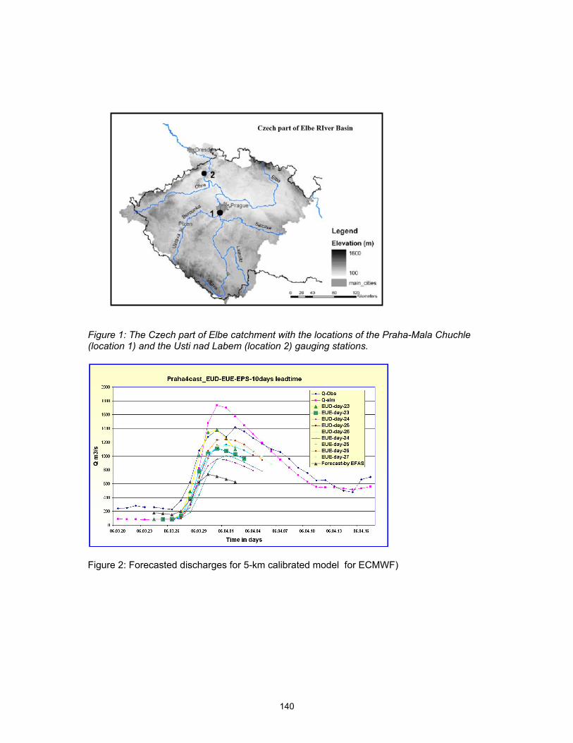
140

Figure 1: The Czech part of Elbe catchment with the locations of the Praha-Mala Chuchle (location 1) and the Usti nad Labem (location 2) gauging stations.

Figure 2: Forecasted discharges for 5-km calibrated model for ECMWF)

141

European Commission

EUR 22861EN – Joint Research Centre – Institute for Environment and Sustainability Title: 3rd HEPEX workshop, Book of abstracts Editors: J. Thielen, J. Bartholmes and J. Schaake Luxembourg: Office for Official Publications of the European Communities 2007EUR – Scientific and Technical Research series – ISSN 1018-5593

AbstractThis Book of Abstracts is a collection of abstracts presented during the 3rd HEPEX workshop

held at Stresa from 27th to 29th June 2007.

Specific sessions of the workshop address the following subjects:

• HEPEX testbeds, datasets and forecast tools

• Ensemble weather and climate forecast applications

• Hydrologic ensemble processing

• Best practice for analyzing and visualizing uncertainty

• User perspectives

The 3rd HEPEX workshop has been organised and coordinated jointly by HEPEX, the

Hydrologic Ensemble Prediction Experiment and the European Commission, Joint Research

Center, Ispra, Italy

The mission of the JRC is to provide customer-driven scientific and technical supportfor the conception, development, implementation and monitoring of EU policies. As a service of the European Commission, the JRC functions as a reference centre of science and technology for the Union. Close to the policy-making process, it serves the common interest of the Member States, while being independent of special interests, whether private or national.