Embed Size (px)
Citation preview
Climate change impacts in EuropeFinal report of the PESETA research project
Juan-Carlos Ciscar (editor)
EUR 24093 EN - 2009
The mission of the IPTS is to provide customer-driven support to the EU policy-making process by researching science-based responses to policy challenges that have both a socio-economic and a scientific or technological dimension.
The mission of the JRC-IES is to provide scientific-technical support to the European Union’s policies for the protection and sustainable development of the European and global environment.
European Commission Joint Research Centre Institute for Prospective Technological Studies Institute for Environment and Sustainability Contact information Address: Edificio Expo. c/ Inca Garcilaso, 3. E-41092 Seville (Spain) E-mail: [email protected] Tel.: +34 954488318 Fax: +34 954488300 http://ipts.jrc.ec.europa.eu http://www.jrc.ec.europa.eu Legal Notice Neither the European Commission nor any person acting on behalf of the Commission is responsible for the use which might be made of this publication. A great deal of additional information on the European Union is available on the Internet. It can be accessed through the Europa server http://europa.eu/ JRC 55391 EUR 24093 EN ISSN 1018-5593 ISBN 978-92-79-14272-7 DOI 10.2791/32500 Luxembourg: Office for Official Publications of the European Communities © European Communities, 2009 Reproduction is authorised provided the source is acknowledged Printed in Spain
Authors
Scientific coordination
Juan-Carlos Ciscar (Institute for Prospective Technological Studies-Joint Research Center, IPTS-JRC)
Antonio Soria (IPTS-JRC).
Climate scenarios
Clare M. Goodess (Climatic Research Unit, University of East Anglia)
Ole B. Christensen (Danish Meteorological Institute).
Agriculture study
Ana Iglesias (Department of Agricultural Economics and Social Sciences, Polytechnic University of Madrid)
Luis Garrote (Department of Civil Engineering, Polytechnic University of Madrid)
Marta Moneo (Potsdam Institute for Climate Impact Research, PIK)
Sonia Quiroga (Department of Statistics, Alcala University).
River flood study
Luc Feyen (Institute for Environment and Sustainability-Joint Research Center, IES-JRC)
Rutger Dankers (Met Office Hadley Centre).
Coastal systems study
Robert Nicholls (School of Civil Engineering & the Environment, University of Southampton)
Julie Richards (ABP Marine Environmental Research Ltd)
Francesco Bosello (Milan University, FEEM)
Roberto Roson (Ca'Foscari University).
Tourism study
Bas Amelung (ICIS, Maastricht University)
Alvaro Moreno (ICIS, Maastricht University).
Human Health study
Paul Watkiss (Paul Watkiss Associates, PWA)
Alistair Hunt (Metroeconomica)
Stephen Pye (AEA Technology)
Lisa Horrocks (AEA Technology).
Integration into the general equilibrium model
Juan-Carlos Ciscar (IPTS-JRC)
László Szabó (IPTS-JRC)
Denise van Regemorter (IPTS-JRC)
Antonio Soria (IPTS-JRC).
PESETA final report 3 JRC/IPTS – JRC/IES

PESETA final report 5 JRC/IPTS – JRC/IES
Acknowledgements
This work was funded by the European Commission (EC) Joint Research Center (JRC) project
PESETA (Projection of Economic impacts of climate change in Sectors of the European Union based
on boTtom-up Analysis). It largely benefited from past EC DG Research projects, in particular from
the following projects: PRUDENCE, DINAS-COAST, NewExt and cCASHh. We acknowledge the
PRUDENCE project and the Rossby Center for providing climate data.
We want to acknowledge the fruitful comments, constructive participation and generous contribution
of the members of the PESETA Advisory and Review Board all along the various stages of the
project: Tim Carter (the Finnish Environment Institute, SYKE), Wolfgang Cramer (Potsdam Institute
for Climate Impact Research, PIK), Sam Fankhauser (London School of Economics), Dennis Tirpak
(World Resources Institute), and John Mac Callaway (UNEP, Risø Centre).
We thank the support received from the European Commission services, in particular, DG
Environment: Artur Runge-Metzger, Ger Klaassen, Tom van Ierland, Jacques Delsalle, Lieve van
Camp, Abigail Howells, and Jane Amilhat; DG Research: Elisabeth Lipiatou, Wolfram Schrimpf, Lars
Müller, Marta Moren-Abat, Denis Peter, Geogrios Amanatidis, and Jeremy Bray.
JRC-IPTS staff was actively involved in the review of the draft reports of the study. We acknowledge
the contribution of Gillaume Leduc, Françoise Némry, Ignacio Hidalgo, Gabriella Németh and
Wojciech Suwala, and the comments received from Peter Kind, Bert Saveyn, Andries Brandsma,
Ignacio Pérez, and Marc Mueller. We also thank Catharina Bamps (JRC-IPTS) and Katalin Bódis
(JRC-IES) for work on climate data and maps
We would like also to acknowledge the comments and suggestions received from Carlos Abanades
(Consejo Superior de Investigaciones Científicas), Luis Balairón (Agencia Estatal de Meteorología),
Salvador Barrios (DG ECFIN, European Commission), Michael Hanemann (University of California
Berkeley), Stéphane Isoard (European Environment Agency, EEA), André Jol (EEA), Nikos
Kouvaritakis (National Technical University of Athens, NTUA), Sari Kovats (London School of
Hygiene and Tropical Medicine), Robert Mendelsohn (Yale University), Leonidas Paroussos (NTUA),
Ronan Uhel (EEA) and David Viner (University of East Anglia).
Previous versions of this study were presented at the following international energy conferences:
International Energy Workshop (IEW) 2007; IEW 2008; IARU 2009 International Scientific Congress
on Climate Change, Copenhagen; International Seminar on macroeconomic assessment of climate
change impacts, St. Petersburg, June 2009. We acknowledge comments received from the participants.

PESETA final report 7 JRC/IPTS – JRC/IES
Preface The April 2009 EC White Paper on adaptation notes the need to better know the possible
consequences of climate change in Europe. The main objective of the PESETA (Projection of
Economic impacts of climate change in Sectors of the European Union based on boTtom-up Analysis)
project is to contribute to a better understanding of the possible physical and economic impacts
induced by climate change in Europe over the 21st century in the following aspects: agriculture, river
basin floods, coastal systems, tourism, and human health.
This research project has followed an innovative, integrated approach combining high resolution
climate and sectoral impact models with comprehensive economic models, able to provide first
estimates of the impacts for alternative climate futures. This approach has been implemented for the
first time in Europe. The project has implied truly multidisciplinary work (including e.g. climate
modelling, agronomic and civil engineering, health and economics), leading to conclusions that could
not have been derived from the scientific disciplines in isolation.
This project illustrates well the Joint Research Centre (JRC)'s mission of supporting EU policymakers
by developing science-based responses to policy challenges. The JRC has entirely financed the project
and has played a key role in the conception and execution of the project. Two JRC institutes, the
Institute for Prospective Technological Studies (IPTS) and the Institute for Environment and
Sustainability (IES), contributed to this study. The JRC-IPTS coordinated the project and the JRC-IES
made the river floods impact assessment. The integration of the market impacts under a common
economic framework was made at JRC-IPTS using the GEM-E3 model.
Early results of the project have been used by DG Environment both as evidence of impacts
concerning the justification of greenhouse gas mitigation policies (2007 Communication) and as first
results on potential impacts, providing useful insights for the conception of adaptation policies at a
pan-European scale, in the context of the Green Paper on Adaptation (July 2007) and the White Paper
on Adaptation (April 2009).
The main purpose of this publication is to summarise the project methodology and present the main
results, which can be relevant for the current debate on prioritising adaptation policies within Europe.
A series of technical publications, including the various aspects of this integrated assessment,
accompanies this summary report (please visit http://peseta.jrc.ec.europa.eu/).
Peter Kind Leen Hordijk
IPTS Director IES Director

Table of contents
EXECUTIVE SUMMARY...........................................................................................17
1 OVERVIEW OF THE PESETA PROJECT .......................................................23 1.1 Project organisation..................................................................................................................................23 1.2 Motivation and objective of the study.....................................................................................................23 1.3 Scope of the assessment ............................................................................................................................24 1.4 The PESETA project methodology: innovative issues ..........................................................................25 1.5 Overview of this report.............................................................................................................................27
2 METHODOLOGICAL FRAMEWORK...............................................................29 2.1 Introduction ..............................................................................................................................................29 2.2 Grouping of countries...............................................................................................................................29 2.3 Scenarios....................................................................................................................................................31
2.3.1 Socioeconomic scenarios.................................................................................................................31 2.3.2 Climate scenarios.............................................................................................................................32 2.3.3 Climate data needs of the sectoral assessments ...............................................................................37 2.3.4 Overview of scenarios in each impact category ..............................................................................38
2.4 Adaptation.................................................................................................................................................39 2.5 Economic assessment................................................................................................................................40
2.5.1 Discounting .....................................................................................................................................40 2.5.2 Valuation methods: direct economic effects....................................................................................40 2.5.3 Valuation methods: overall economic (general equilibrium) effects...............................................41
3 AGRICULTURE IMPACT ASSESSMENT........................................................43 3.1 Agriculture integrated methodology .......................................................................................................43
3.1.1 The modelling approach ..................................................................................................................43 3.1.2 Limitations and uncertainties...........................................................................................................44
3.2 Physical impacts........................................................................................................................................45 3.3 Economic impacts .....................................................................................................................................49
4 RIVER FLOODS ASSESSMENT......................................................................51 4.1 Modelling floods in river basins...............................................................................................................51
4.1.1 The modelling approach ..................................................................................................................51 4.1.2 Limitations and uncertainties...........................................................................................................52
4.2 Physical impacts........................................................................................................................................52 4.3 Economic impacts .....................................................................................................................................54
5 COASTAL SYSTEMS ASSESSMENT .............................................................57 5.1 Modelling approach in coastal systems...................................................................................................57
5.1.1 Coastal system model ......................................................................................................................57
PESETA final report 9 JRC/IPTS – JRC/IES
5.1.2 Limitations and uncertainties...........................................................................................................58 5.2 Physical impacts........................................................................................................................................58 5.3 Economic impacts .....................................................................................................................................63
5.3.1 Direct economic effects ...................................................................................................................63 5.3.2 Overall (general equilibrium) economic effects ..............................................................................64
6 TOURISM ASSESSMENT................................................................................67 6.1 Tourism impact methodology ..................................................................................................................67
6.1.1 The modelling approach ..................................................................................................................67 6.1.2 Limitations and uncertainties...........................................................................................................68
6.2 Physical impacts........................................................................................................................................68 6.2.1 Changes in Tourism Climate Index between the 1970s and the 2020s............................................69 6.2.2 Changes in Tourism Climate Index between the 1970s and the 2080s............................................71 6.2.3 Changes in bed nights in the 2080s .................................................................................................78
6.3 Economic impacts .....................................................................................................................................79 6.3.1 Base case: flexible overall EU and seasonal demand ......................................................................79 6.3.2 Fixed overall EU demand and flexible seasonal demand ................................................................80 6.3.3 Fixed overall EU demand and fixed seasonal demand ....................................................................80
7 HUMAN HEALTH ASSESSMENT....................................................................83 7.1 Human health model ................................................................................................................................83
7.1.1 Modelling approach.........................................................................................................................83 7.1.2 Limitations and uncertainties...........................................................................................................87
7.2 Physical impacts........................................................................................................................................88 7.2.1 Mortality changes in the 2020s........................................................................................................89 7.2.2 Mortality changes in the 2080s........................................................................................................91
7.3 Economic impacts .....................................................................................................................................97
8 INTEGRATED ECONOMIC ASSESSMENT OF MARKET IMPACTS: THE GEM-E3 PESETA MODEL ...............................................................................99
8.1 Introduction ..............................................................................................................................................99 8.2 Methodology of integration......................................................................................................................99 8.3 Effect of 2080s climate in the current economy....................................................................................101 8.4 Potential impacts and adaptation ..........................................................................................................101 8.5 Overview of physical impacts ................................................................................................................102 8.6 The GEM-E3 PESETA model ...............................................................................................................103 8.7 Integration of impacts into the GEM-E3 PESETA Model..................................................................104 8.8 Economic Impact Results.......................................................................................................................105
8.8.1 Welfare effects of climate change in Europe.................................................................................105 8.8.2 GDP effects ...................................................................................................................................108
9 CONCLUSIONS..............................................................................................111 9.1 Main Findings .........................................................................................................................................111
PESETA final report 10 JRC/IPTS – JRC/IES
PESETA final report 11 JRC/IPTS – JRC/IES
9.2 Caveats and Uncertainties......................................................................................................................114 9.3 Further research .....................................................................................................................................116
10 REFERENCES................................................................................................117
11 ANNEX. RESULTS FOR THE EU AND EUROPEAN REGIONS...................125

List of tables
Table 1. Overview of the main driving forces........................................................................................................32
Table 2. The PESETA climate scenarios ...............................................................................................................32
Table 3. Global and EU temperature increase (2071-2100, compared to 1961-1990) ...........................................33
Table 4. Summary of socio-economic and climate scenarios ................................................................................34
Table 5. Global sea-level rise scenarios at 2100 ....................................................................................................37
Table 6. PESETA climate data needs by sector .....................................................................................................38
Table 7. Socio-economic and climate signals across impact studies .....................................................................38
Table 8. Cases analysed per sector.........................................................................................................................39
Table 9. Agriculture: crop yield changes (%), compared to the 1961-1990 period ...............................................46
Table 10. Agriculture: regional aggregation ..........................................................................................................49
Table 11. River floods: expected annual population affected (1000s/year) ...........................................................54
Table 12. River floods: expected economic damage (million €/year)....................................................................54
Table 13. Global sea-level rise scenarios ...............................................................................................................58
Table 14. Coastal systems: people flooded (1000s/year) in main scenarios with high climate sensitivity, without adaptation ........................................................................................................................................60
Table 15. Coastal systems: EU Aggregated Results for IPCC A2 Economic Impacts, Highest Sea-level Rise (million €/year) (1995 values) .........................................................................................................63
Table 16. Coastal systems: EU Aggregated Results for IPCC B2 Economic Impacts, Lowest Sea-level Rise (million €/year) (1995 values) .........................................................................................................64
Table 17. Coastal systems: industrial disaggregation of the CGE model...............................................................65
Table 18. Coastal systems: A2 Scenario, High Sea-level Rise 2085. Main Macroeconomic Effects (no adaptation) .......................................................................................................................................65
Table 19. Coastal systems: A2 Scenario, High Sea-level Rise, 2085. Main Macroeconomic Effects (optimal adaptation) .......................................................................................................................................66
Table 20. Tourism: simulated changes in bed nights in the 2080s (compared to the 1970s) and 2005 bed nights 78
Table 21. Tourism: change in expenditure receipts in the 2080s, central case (million €) ....................................80
Table 22. Tourism: change in expenditure receipts in the 2080s, annual case (million €).....................................80
Table 23. Tourism: change in expenditure receipts in the 2080s, annual case (million €).....................................81
Table 24. Human health: heat-related and cold-related mortality rate projections for the 2020s - death rate (per 100,000 population per year)...........................................................................................................89
PESETA final report 13 JRC/IPTS – JRC/IES
PESETA final report 14 JRC/IPTS – JRC/IES
Table 25. Human health: heat-related mortality rate projections for the 2080s - - death rate (per 100,000 population per year).........................................................................................................................92
Table 26. Human health: cold-related mortality rate projections for the 2080s - - death rate (per 100,000 population per year).........................................................................................................................92
Table 27. Human health: economic valuation of mortality effects in all scenarios................................................98
Table 28. Physical annual impacts in agriculture, river basins, coastal systems and tourism of 2080s climate change scenarios in the current European economy ......................................................................103
Table 29. Household welfare annual effects in all impact categories for 2080s climate change scenarios in the current European economy............................................................................................................106
Table 30. Annual economic impacts in agriculture, river basins, tourism and coastal systems for 2080s climate change scenarios in the current European economy ......................................................................109
Table 31. Summary of results for the EU.............................................................................................................125 U
Table 32. Summary of results for Northern Europe.............................................................................................126
Table 33. Summary of results for British Isles.....................................................................................................127
Table 34. Summary of results for Central Europe North .....................................................................................128
Table 35. Summary of results for Central Europe South .....................................................................................129
Table 36. Summary of results for Southern Europe.............................................................................................130
List of figures Figure 1. Grouping of EU countries in the study ...................................................................................................30
Figure 2. European land temperature (°C) .............................................................................................................33
Figure 3. Projected 2080s changes in mean annual temperature............................................................................35
Figure 4. Projected 2080s changes in annual precipitation ....................................................................................36
Figure 5. Agriculture: crop yield changes of the 2.5°C scenario (2080s) ..............................................................46
Figure 6. Agriculture: crop yield changes of the 3.9°C scenario (2080s) ..............................................................47
Figure 7. Agriculture: crop yield changes of the 4.1°C scenario (2080s) ..............................................................47
Figure 8. Agriculture: crop yield changes of the 5.4°C scenario (2080s) ..............................................................48
Figure 9. Agriculture: crop yield changes of the 2020s scenario ...........................................................................48
Figure 10. Agriculture: GDP changes under the climate change scenarios ...........................................................50
Figure 11. River floods: relative change in 100-year return level of river discharge between scenario (2071-2100) and control period (1961-1990) for the 3.9ºC (left) and 2.5ºC (right) scenarios .............................53
Figure 12. River floods: relative change in expected annual direct damage (averaged over administrative level NUTS2) between scenario (2071-2100) and control period (1961-1990) for the 2.5ºC scenario....55
Figure 13. River floods: relative change in expected annual direct damage (averaged over administrative level NUTS2) between scenario (2071-2100) and control period (1961-1990) for the 3.9ºC scenario....56
Figure 14. Coastal systems: comparison of DIVA outputs for land loss in the EU under the A2 storyline without adaptation ........................................................................................................................................59
Figure 15. Coastal systems: comparison of DIVA estimates of the number of people flooded in the EU with and without adaptation by 2085 .............................................................................................................60
Figure 16. Coastal systems: baseline results for people actually flooded (1000s/year) across Europe..................61
Figure 17. Coastal systems: people actually flooded (1000s/year) across Europe, for the B2 scenario, 2085 (ECHAM4; 4.1°C), without adaptation ...........................................................................................62
Figure 18. Coastal systems: people actually flooded (1000s/year) across Europe, for the A2 scenario, 2085 (ECHAM4, 5.4°C), without adaptation ...........................................................................................62
Figure 19. Tourism: TCI scores in spring (top), summer (middle) and autumn (bottom) in the 1970s (left) and the 2020s (right) according to the Rossby Centre RCA3 model ...........................................................70
Figure 20. Tourism: TCI scores in spring in the 1970s (left) and the 2080s (right), according to the HIRHAM model, 3.9°C scenario (top) and 2.5°C scenario (bottom)...............................................................71
Figure 21. Tourism: TCI scores in spring in the 1970s (left) and the 2080s (right), according to the RCAO model, 5.4°C scenario (top) and 4.1°C scenario (bottom)...............................................................72
Figure 22. Tourism: TCI scores in summer in the 1970s (left) and the 2080s (right), according to the HIRHAM model, 3.9°C scenario (top) and 2.5°C scenario (bottom)...............................................................73
Figure 23. Tourism: TCI scores in summer in the 1970s (left) and the 2080s (right), according to the RCAO model, 5.4°C scenario (top) and 4.1°C scenario (bottom)...............................................................73
PESETA final report 15 JRC/IPTS – JRC/IES
PESETA final report 16 JRC/IPTS – JRC/IES
Figure 24. Tourism: TCI scores in autumn in the 1970s (left) and the 2080s (right), according to the HIRHAM model, 3.9°C scenario (top) and 2.5°C scenario (bottom)...............................................................74
Figure 25. Tourism: TCI scores in autumn in the 1970s (left) and the 2080s (right), according to the RCAO model, 5.4°C scenario (top) and 4.1°C scenario (bottom)...............................................................75
Figure 26. Tourism: TCI scores in winter in the 1970s (left) and the 2080s (right), according to the HIRHAM model, 3.9°C scenario (top) and 2.5°C scenario (bottom)...............................................................76
Figure 27. Tourism: TCI scores in winter in the 1970s (left) and the 2080s (right), according to the RCAO model, 5.4°C scenario (top) and 4.1°C scenario (bottom)...............................................................76
Figure 28. Tourism: Average number of months per year with very good conditions or better (TCI>70), in the 1970s (left) and the 2080s (right), according to the 3.9°C scenario (top) and 2.5°C scenario (bottom) ...........................................................................................................................................77
Figure 29. Tourism: Average number of months per year with very good conditions or better (TCI>70), in the 1970s (left) and the 2080s (right), according to the RCAO model, 5.4°C scenario (top) and 4.1°C scenario (bottom).............................................................................................................................78
Figure 30. Human health: Illustrative uncertainty for temperature related health quantification and valuation ....87
Figure 31. Human health: population (left) and annual deaths (right) in Europe for 2080s (3.9°C scenario)........88
Figure 32. Human health: average annual heat-related (left) and cold-related (right) death rates per 100,000 population, for the 2020s, using the climate-dependent health functions (no acclimatisation) .......90
Figure 33. Human health: average annual heat-related (left) and cold-related (right) death rates per 100,000 population, for the 2020s, using the country-specific health functions (no acclimatisation)...........91
Figure 34. Human health: average annual heat-related (left) and cold-related (right) death rates per 100,000 population, for the 2080s, 2.5°C scenario, using climate-dependent health functions (no acclimatisation)................................................................................................................................93
Figure 35. Human health: average annual heat-related (left) and cold-related (right) death rates per 100,000 population, for the 2080s, 2.5°C scenario, using country-specific health functions (no acclimatisation)................................................................................................................................93
Figure 36. Human health: average annual heat-related (left) and cold-related (right) death rates per 100,000 population for the 2080s, 3.9°C scenario, using climate-dependent health functions (no acclimatisation)................................................................................................................................95
Figure 37. Human health: average annual heat-related (left) and cold-related (right) death rates per 100,000 population for the 2080s, 3.9°C scenario, using country-specific health functions (no acclimatisation)................................................................................................................................95
Figure 38. Human health: Overview of mortality changes in all scenarios for a range of projections, models, functions and with and without acclimatisation. Top – heat related: Bottom- cold related effects .96
Figure 39. The PESETA Integrated approach......................................................................................................100
Figure 40. 2080s climate in the current European economy: sectoral decomposition of annual household welfare changes for the EU and European regions.....................................................................................107
Figure 41. Annual damage in terms of GDP loss (million €)...............................................................................112
Figure 42. Annual damage in terms of welfare change (%).................................................................................112
Figure 43. Sectoral decomposition of regional welfare changes..........................................................................113
Executive Summary
Policy context
The international community is seeking agreement on post-2012 climate mitigation policies aimed at
reducing global greenhouse gas (GHG) emissions. The European Union (EU) has proposed to limit the
global temperature increase to 2°C above pre-industrial levels and has endorsed a commitment to
cutting GHG emissions by at least 20% by 2020 compared to 1990 levels. The G8 have supported a
GHG emission reduction goal for developed countries of at least 80% by 2050. Adaptation policies to
minimise adverse impacts of climate change and to take advantage of existing opportunities will also
be key in post-2012 climate policies.
The avoidance of environmental and economic damages and adverse effects on human health is the
ultimate justification of more stringent climate policies. Yet little is known about the potential impacts
of climate change on the European environment, human health and economy with respect to different
sectors and geographical regions. Such information is necessary to design and prioritise adaptation
strategies, as stressed by the European Commission (EC) White Paper on Adaptation.
Purpose and scope
The PESETA project makes the first regionally-focused multi-sectoral integrated assessment of the
impacts of climate change in the European economy. The project also suggests an innovative
modelling framework able to provide useful insights for adaptation policies on a pan-European scale,
with the geographical resolution relevant to national stakeholders.
Five impact categories have been addressed: agriculture, river floods, coastal systems, tourism, and
human health. These aspects are highly sensitive to changes in mean climate and climate extremes.
The approach enables a comparison between the impact categories and therefore provides a notion of
the relative severity of the damage inflicted. For the climate scenarios of the study, two time frames
have been considered: the 2020s and the 2080s. The study evaluates the economic effects of future
climate change on the current economy.
Other key impacts, such as effects on forestry, impacts in ecosystems and biodiversity and catastrophic
events, have not yet been analysed. Therefore, the PESETA project underestimates the impacts of
climate change in Europe to a large extent.
Methodology
Several research studies have estimated or employed climate damage functions as reduced-form
formulations linking climate variables to economic impacts (usually average global temperature to
gross domestic product, GDP). However, for assessing impacts and prioritising adaptation policies,
such an approach has three disadvantages: (1) estimates are based on results from the literature coming
PESETA final report 17 JRC/IPTS – JRC/IES

from different, and possibly inconsistent, climate scenarios; (2) only average temperatures and
precipitation are used, not considering other relevant climate variables and the required time-space
resolution in climate data; (3) impact estimates lack the relevant resolution and sector-specific details.
PESETA has put forward an innovative methodology integrating (a) high time-space resolution
climate data, (b) impact-specific models, which use common climate scenarios, and (c) a multi-
sectoral computable general equilibrium (CGE) economic model, estimating the effects of climate
change impacts on the overall economy.
Climate data, physical impact models and an economic model are integrated under a consistent
methodological framework following three steps. In the first stage, daily and 50 x 50 km resolution
(approximately the size of London) climate data are selected for a series of future climate scenarios. In
the second step, these data serve as input to run the physical impact models for the five impact
categories. The DSSAT crop models have been used to quantify the physical impacts on agriculture, in
terms of yield changes of selected crops. Estimates of changes in the frequency and severity of river
floods are based on simulations with the LISFLOOD model. Impacts of sea level rise (SLR) on coastal
systems (e.g. sea floods) have been quantified with the DIVA model. The tourism study has modelled
the changes in major international tourism flows within Europe assessing the relationship between bed
nights and a climate-related index of human comfort. The human health assessment has been made
using evidence about exposure-response functions, linking temperature to mortality. Heatwaves are
not considered.
In the third stage, the market impact categories (those with market prices, i.e. agriculture, river floods,
coastal systems and tourism) and their associated direct economic effects are introduced into a
computable general equilibrium (CGE) model, the GEM-E3 Europe model, modelling individually
most EU countries (Cyprus, Luxemburg and Malta are not included). This framework captures not
only the direct effects of a climate impact on a particular region and sector but also the transmission of
these effects to the rest of the economy. The CGE model ultimately translates the climate change
scenarios into consumer welfare and GDP changes, compared to the baseline scenario without climate
change.
The EU has been divided into five regions to simplify interpretation: Southern Europe (Portugal,
Spain, Italy, Greece, and Bulgaria), Central Europe South (France, Austria, Czech Republic, Slovakia,
Hungary, Romania, and Slovenia), Central Europe North (Belgium, The Netherlands, Germany, and
Poland), British Isles (Ireland and UK), and Northern Europe (Sweden, Finland, Estonia, Latvia, and
Lithuania). The main criteria for grouping countries are the geographical position and the economic
size.
It should be noted that this project did not intend to produce forecasts of the impacts of climate
change, but rather simulations under alternative future climate scenarios.
PESETA final report 18 JRC/IPTS – JRC/IES
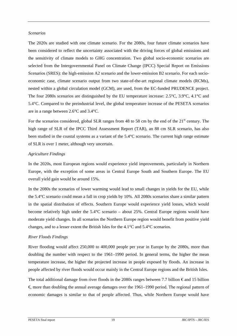
Scenarios
The 2020s are studied with one climate scenario. For the 2080s, four future climate scenarios have
been considered to reflect the uncertainty associated with the driving forces of global emissions and
the sensitivity of climate models to GHG concentration. Two global socio-economic scenarios are
selected from the Intergovernmental Panel on Climate Change (IPCC) Special Report on Emissions
Scenarios (SRES): the high-emission A2 scenario and the lower-emission B2 scenario. For each socio-
economic case, climate scenario output from two state-of-the-art regional climate models (RCMs),
nested within a global circulation model (GCM), are used, from the EC-funded PRUDENCE project.
The four 2080s scenarios are distinguished by the EU temperature increase: 2.5°C, 3.9°C, 4.1°C and
5.4°C. Compared to the preindustrial level, the global temperature increase of the PESETA scenarios
are in a range between 2.6°C and 3.4°C.
For the scenarios considered, global SLR ranges from 48 to 58 cm by the end of the 21st century. The
high range of SLR of the IPCC Third Assessment Report (TAR), an 88 cm SLR scenario, has also
been studied in the coastal systems as a variant of the 5.4°C scenario. The current high range estimate
of SLR is over 1 meter, although very uncertain.
Agriculture Findings
In the 2020s, most European regions would experience yield improvements, particularly in Northern
Europe, with the exception of some areas in Central Europe South and Southern Europe. The EU
overall yield gain would be around 15%.
In the 2080s the scenarios of lower warming would lead to small changes in yields for the EU, while
the 5.4°C scenario could mean a fall in crop yields by 10%. All 2080s scenarios share a similar pattern
in the spatial distribution of effects. Southern Europe would experience yield losses, which would
become relatively high under the 5.4°C scenario – about 25%. Central Europe regions would have
moderate yield changes. In all scenarios the Northern Europe region would benefit from positive yield
changes, and to a lesser extent the British Isles for the 4.1°C and 5.4°C scenarios.
River Floods Findings
River flooding would affect 250,000 to 400,000 people per year in Europe by the 2080s, more than
doubling the number with respect to the 1961–1990 period. In general terms, the higher the mean
temperature increase, the higher the projected increase in people exposed by floods. An increase in
people affected by river floods would occur mainly in the Central Europe regions and the British Isles.
The total additional damage from river floods in the 2080s ranges between 7.7 billion € and 15 billion
€, more than doubling the annual average damages over the 1961–1990 period. The regional pattern of
economic damages is similar to that of people affected. Thus, while Northern Europe would have
PESETA final report 19 JRC/IPTS – JRC/IES
fewer damages, the Central Europe area and the British Isles would undergo significant increases in
expected damages.
Coastal Systems Findings
The number of people annually affected by sea floods in the reference year (1995) is estimated to be
36,000. Without adaptation, the number of people affected annually by flooding increases significantly
in all scenarios, in the range of 775,000 to 5.5 million people. The British Isles, the Central Europe
North and Southern Europe regions would be the areas potentially most affected by coastal floods.
However, when adaptation is taken into account (dikes and beach nourishment) the number of people
exposed to floods are significantly reduced.
The economic costs to people who might migrate due to land loss (through submergence and erosion)
are also substantially increased under a high rate of sea-level rise, assuming no adaptation, and
increase over time. When adaptation measures are implemented (building dikes), this displacement of
people becomes a minor impact, showing the important benefit of adaptation to coastal populations
under rising sea levels.
Tourism Findings
Concerning the 2020s, in the three main seasons (i.e. spring, summer and autumn) climate conditions
for outdoor tourism improve in most areas of Europe. Changes are most significant in the
Mediterranean region, where the area with very good to ideal conditions increases.
On the contrary, for the 2080s, the distribution of climatic conditions in Europe is projected to change
significantly. For the spring season, all climate model results show a clear extension towards the North
of the zone under good conditions. Excellent conditions in spring, which are mainly found in Spain in
the baseline period, would spread across most of the Mediterranean coastal areas by the 2080s.
Changes in autumn are more or less comparable to the ones in spring. In summer, the zone of good
conditions also expands towards the North, but this time at the expense of the South, where climatic
conditions would deteriorate.
When other determinants are considered, such as price and income levels, it is possible to estimate the
changes in expenditure associated with bed nights. There would be additional expenditures, with a
relatively small EU-wide positive impact. Southern Europe, which currently accounts for more than
half of the total EU capacity of tourist accommodation, would be the only region with a decline in bed
nights, estimated to be in a range between 1% and 4%, depending on the climate scenario. The rest of
Europe is projected to have large increases in bed nights, in the range of 15% to 25% for the two
warmest scenarios.
PESETA final report 20 JRC/IPTS – JRC/IES
Human Health Findings
In the 2020s, without adaptation measures and acclimatisation, the estimated increases in heat-related
mortality are projected to be lower than the estimated decrease in cold-related mortality. The potential
increase in heat-related mortality in Europe could be over 25,000 extra deaths per year, with the rate of
increase potentially higher in Central Europe South and Southern European regions. However,
physiological and behavioural responses to the warmer climate would have a very significant effect in
reducing this mortality (acclimatisation), potentially reducing the estimates by a factor of five to ten. It
is also possible that there may be a decline in the sensitivity of mortality to cold, though this is more
uncertain.
By the 2080s, the effect of heat- and cold-related mortality changes depends on the set of exposure-
response and acclimatisation functions used. The range of estimates for the increase in mortality is
between 60,000 and 165,000 (without acclimatisation), again decreasing by a factor of five or more if
acclimatisation is included. The range of estimates for the decrease in cold-related mortality is
between 60,000 and 250,000, though there may also be a decline in the sensitivity of mortality to cold.
Overall economic impacts in Europe
The consequences of climate change in the four market impact categories (i.e. agriculture, river floods,
coastal systems and tourism) can be valued in monetary terms as they directly affect sectoral markets
and – via the cross-sector linkages – the overall economy. They also influence the consumption
behaviour of households and therefore their welfare.
The analysis of potential impacts of climate change, defined as impacts that might occur without
considering public adaptation, can allow the identification of priorities in adaptation policies across
impact categories and regional areas. If the climate of the 2080s occurred today, the annual damage of
climate change to the EU economy in terms of GDP loss is estimated to be between 20 billion € for the
2.5°C scenario and 65 billion € for the 5.4°C scenario with high SLR.
Yet the damages in GDP terms underestimate the actual losses. For instance, the repairing of damages
to buildings due to river floods increase production (GDP), but not consumer welfare. The aggregated
impact on the four categories would lead to an EU annual welfare loss of between 0.2% for the 2.5°C
scenario and 1% for the 5.4°C scenario, variant with a high SLR (88cm). The historic EU annual
growth of welfare is around 2%. Thus climate change could reduce the annual welfare improvement
rate to between 1.8% (for the scenario with a 0.2% welfare loss) and 1% (for the scenario with a 1%
welfare loss).
EU-aggregated economic impact figures hide a high variation across regions, climate scenarios and
impact categories. In all 2080s scenarios, most regions would undergo welfare losses, with the
exception of Northern Europe, where gains are in a range of 0.5% to 0.8% per year, largely driven by
PESETA final report 21 JRC/IPTS – JRC/IES
PESETA final report 22 JRC/IPTS – JRC/IES
the improvement in agricultural yields. Southern Europe could be severely affected by climate change,
with annual welfare losses around 1.4% for the 5.4°C scenario.
The sectoral and geographical decomposition of welfare changes under the 2.5°C scenario shows that
aggregated European costs of climate change are highest for agriculture, river flooding and coastal
systems, much larger than for tourism. The British Isles, Central Europe North and Southern Europe
appear the most sensitive areas. Moreover, moving from a European climate future of 2.5°C to one of
3.9°C aggravates the three noted impacts in almost all European regions. In the Northern Europe area,
these impacts are offset by the increasingly positive effects related to agriculture.
The 5.4°C scenario leads to an annual EU welfare loss of 0.7%, with more pronounced impacts in
most sectors in all EU regions. The agricultural sector is the most important impact category in the EU
average; the significant damages in Southern Europe and Central Europe South are not compensated
for by the gains in Northern Europe. Impacts from river flooding are also more important in this case
than in the other scenarios, with particular aggravation in the British Isles and in Central Europe. In
the 5.4°C scenario variant with the high SLR (88 cm), which would lead to a 1% annual welfare loss
in the EU, coastal systems would become the most important impact category, especially in the British
Isles.
Further research
The proposed methodology is complex and subject to many caveats and uncertainties. Studying other
sectors (such as transport and energy), non–market effects (e.g. loss in biodiversity), climate
variability related damages, catastrophic damages, the cost-benefit analysis of adaptation, and
considering land-use scenarios deserves additional research efforts, as well as broadening the set of
climatic scenarios in order to better reflect climate modelling uncertainties.
1 OVERVIEW OF THE PESETA PROJECT
1.1 Project organisation
PESETA was coordinated by JRC/IPTS (Economics of Energy, Climate Change and Transport Unit)
and involved ten research institutes (University of East Anglia, Danish Meteorological Institute,
Polytechnic University of Madrid, JRC/IES, University of Southampton, FEEM, ICIS-Maastricht
University, AEA Technology, Metroeconomica, and JRC/IPTS). The project also benefitted from the
collaboration of the Rossby Center that kindly provided climate data of a transient climate scenario.
The project has had a multi-disciplinary Advisory and Review Board, composed of renowned experts.
Notably, the PESETA project has largely benefitted from past DG Research projects that developed
both high resolution climate scenarios for Europe and models to project impacts of climate change
(e.g. the DIVA model). In particular, PESETA used climate data provided by the PRUDENCE project
(Christensen et al., 2007) and models and results from the following research projects: DINAS-
COAST, NewExt, and cCASHh.
1.2 Motivation and objective of the study
The international community is looking for an agreement on post-2012 climate mitigation policies
aimed at reducing global greenhouse gas (GHG) emissions. The European Union (EU) has pledged to
limit the global temperature increase to 2°C above pre-industrial levels and has endorsed a
commitment to cutting GHG emissions by at least 20% by 2020 compared to 1990 levels (Council of
the European Union, 2005 and 2007). The leaders of the G8 have more recently (G8, 2009) supported
the goal of developed countries to reduce GHG emissions by at least 80% by 2050. Adaptation
policies to minimise adverse impacts of climate change and to take advantage of existing opportunities
will also be key in post-2012 climate policies.
The avoidance of environmental and economic damages is the ultimate justification of more stringent
climate policies. There are some studies addressing the impacts of climate change in Europe (e.g.
Rotmans et al., 1994; Parry, 2000; Schröter et al., 2005; Alcamo et al., 2007; EEA, 2008). However,
little is known about the potential impacts of climate change on the European economy, in particular
with respect to different economic sectors of interest and geographical regions of concern, necessary
to design and prioritise adaptation strategies, as noted by the European Commission (EC) White Paper
on Adaptation (European Commission, 2009a).
The main motivation of the PESETA project (Projection of Economic impacts of climate change in
Sectors of the European Union based on boTtom-up Analysis) has been to contribute to a better
understanding of the possible physical and economic impacts induced by climate change in Europe
over the 21st century, paying particular attention to the sectoral and geographical dimensions of
PESETA final report 23 JRC/IPTS – JRC/IES
impacts. This follows the recommendation of Stern and Taylor (2007) on following a disaggregated
approach to study the consequences of climate change, concerning different dimensions, places and
times.
The origin of the project dates back to the European Council request (Council of the European Union,
2004) of considering the potential cost of inaction in the field of climate change and, in more general
terms, to enhance the analysis of the benefit aspects of European climate policies in terms of reduction
of potential impacts.
Preliminary results of PESETA have been published in the Staff Working Paper accompanying the EC
Communication on "Limiting Global Climate Change to 2 degrees Celsius. The way ahead for 2020
and beyond" (European Commission, 2007a). Moreover, early results on the impacts for the various
sectors under one specific scenario have been published in the Green Paper "Adapting to climate
change in Europe - options for EU action" (European Commission, 2007b), and in its Annex, as well
as in the 2008 EEA report on impacts (EEA, 2008). The staff working document accompanying the
2009 White Paper on Adaptation (European Commission, 2009a) also contains early results of the
project.
1.3 Scope of the assessment
The scope of the PESETA assessment concerning its time scale, scenarios, geographical coverage and
impacts analysed is presented in what follows and, more in detail, in Chapter 2. Two time windows
have been considered: the 2020s and the 2080s. The 2020s period refers to the middle decade of the
2011-2040 period, while the 2080s relates to the 2071-2100 period. The control period of the study is
1961-1990.
Regarding the 2020s only one climate scenario has been considered, as the climate then is mostly
already determined by past GHG emissions. With respect to the 2080s, four alternative climate futures
have been considered, covering an increase of temperature in Europe in a range of 2.5°C to 5.4°C.
PESETA focuses on the EU and results are presented according to the following breakdown to
simplify interpretation (Section 2.2): Southern Europe (Portugal, Spain, Italy, Greece, and Bulgaria),
Central Europe South (France, Austria, Czech Republic, Slovakia, Hungary, Romania, and Slovenia),
Central Europe North (Belgium, The Netherlands, Germany, and Poland), British Isles (Ireland and
UK), and Northern Europe (Sweden, Finland, Estonia, Latvia, and Lithuania).
In estimating the impacts of climate change five categories have been addressed. Four are market
impact areas: agriculture, river basins, coastal systems, and tourism; and one is a non-market impact
category: human health. This enables a certain comparison between them and therefore provides a
notion of the relative severity of the damage inflicted. For each of these sectoral categories, a
corresponding sectoral-based study is developed by the project partners.
PESETA final report 24 JRC/IPTS – JRC/IES
The five aspects are highly sensitive to changes in mean climate and climate extremes. Agriculture is
the main user of land and water, and still plays a dominant economic role in the rural areas of Europe.
Previous studies (e.g. Alcamo et al., 2007; EEA, 2008) show that the stress imposed by climate
change on agriculture will intensify the regional disparities between European countries.
River floods are the most common natural disaster in Europe (EEA, 2004). Global warming is
generally expected to increase the magnitude and frequency of extreme precipitation events
(Christensen and Christensen, 2003; Frei et al., 2006), which may lead to more intense and frequent
river floods. Coastal regions are areas where wealth and population are concentrated and are
undergoing rapid increases in population and urbanisation (McGranahan et al., 2007). Sea level rise is
a direct threat for productive infrastructures and for the residential and natural heritage zones.
Tourism is a major economic sector in Europe, with the current annual flow of tourists from Northern
to Southern Europe accounting for one in every six tourist arrivals in the world (Mather et al., 2005).
Climate change has the potential to radically alter tourism patterns in Europe by inducing changes in
destinations and seasonal demand structure (Scott et al., 2008).
Human health will be affected by climate change, in direct and indirect ways (Costello et al., 2009).
Effects include changes in temperature-related mortality, food-borne diseases, water-borne diseases
and vector-borne diseases.
This project does not pretend to be comprehensive as relevant impact categories are not included in the
assessment. Market impact categories such as fisheries, forests and energy demand/supply changes
have not yet been addressed. Other non-market impact categories like biodiversity and potentially
catastrophic events are not considered in this study either.
1.4 The PESETA project methodology: innovative issues
There are two kinds of approaches to estimate impacts of climate change: top-down and bottom-up.
Several research studies (e.g. Nordhaus, 1992; Nordhaus and Yang, 1996; Mastrandrea and Schneider
2004; Hitz and Smith, 2004; Stern, 2007) have estimated or employed climate damage functions as
reduced-form formulations linking climate variables to economic impacts (usually average global
temperature to gross domestic product, GDP). An illustration is the recent update of the estimate of the
damage of climate change in the US of the Stern review (Ackerman et al., 2009). These authors
assume that economic and non-economic damages of climate change are a function of temperature:
D = a TN
where D refers to damages, T is the temperature increase and a and N are parameters.
PESETA final report 25 JRC/IPTS – JRC/IES
Indeed, this branch of the literature provided early estimates of the order of magnitude of the effects of
climate change in the world and large regions, as a function of the global temperature change (e.g.
Fankhauser, 1994, 1995; Hitz and Smith, 2004; Tol, 2009).
Yet, for assessing impacts and prioritising adaptation policies such top-down approach has some
disadvantages. Firstly, estimates are based on results from the literature coming from different, and
possibly inconsistent, climate scenarios. Secondly, only average temperature and precipitation are
included, not considering other relevant climate variables and the required time-space resolution in
climate data. Thirdly, and because of the previous point, impact estimates lack the geographical
resolution for adaptation policies. Indeed, aggregate or top-down impact estimates might hide
variability of interest in the regional and sectoral dimensions.
Another strand of the literature has followed a bottom-up approach. This bottom-up or sectoral
approach has been implemented in PESETA, where the physical effects of climate change are
estimated by running high-resolution impact-specific models, which use common selected high-
resolution scenarios of the future climate.
PESETA builds upon examples of assessments made elsewhere, such as the California impact study
(Hayhoe et al., 2004), the US impact studies (e.g. Mendelsohn and Neumann, 1999; Jorgenson et al.,
2004; Ruth et al., 2006), the Russian impact study (Roshydromet, 2005), and the FINADAPT study in
Finland (Carter et al., 2007).
PESETA is indeed the first regionally-focused, quantitative, integrated assessment of the effects of
climate change on vulnerable aspects of the European economy and its overall welfare. The PESETA
project is characterized by a quantitative or model-based assessment of impacts of climate change.
The analysis is innovative because it integrates (a) high space-time resolution climate data, (b) detailed
modelling tools specific for each impact category considered and (c) a multi-sectoral, multi-regional
computable general equilibrium (CGE) economic model. The use of a CGE model to integrate all
market impacts takes into account the indirect economic effects of climate change, in addition to the
direct effects.
Moreover, a key feature of the methodological framework is consistency across the sectoral studies
concerning the use of common socioeconomic and climate scenarios. All studies used the same
datasets. Various approaches to adaptation have been considered, including the non-adaptation case
(Section 2.4).
As noted by Rotmans and Dowlatabadi (1998), the distinctive feature of integrated assessment models,
involving several scientific disciplines, such as that of the PESETA project, is that they can have
added valued compared to a mono-disciplinary assessment.
PESETA final report 26 JRC/IPTS – JRC/IES
PESETA final report 27 JRC/IPTS – JRC/IES
However, it must be noted that quantifying the expected effects of climate change in a very long-term
time horizon requires dealing with many sources of uncertainty, including e.g. future climate,
demographic change, economic development, and technological change. There is poor understanding
of processes (incomplete scientific methodologies) and large gaps in data. Consequently, the results of
the project need to be interpreted with due care and, in particular, are to be considered as 'preliminary'
given the exploratory nature of the PESETA research project.
Despite these limitations, the PESETA project provides a valuable indication of the economic costs of
climate change in Europe based on state-of-the-art physical impact assessment and high-resolution
climate scenarios (daily, 50x50 km grids).
1.5 Overview of this report
This report is divided into nine chapters, including this overview. Chapter 2 presents the main
elements of the methodological framework of the project, including the main features of the climate
scenarios. The following five chapters summarise the methodology of each sectoral assessment and its
main physical and economic results. Chapter 3 deals with the agriculture assessment, chapter 4 with
river floods, chapter 5 with coastal systems, chapter 6 with tourism and chapter 7 with human health.
Chapter 8 synthesises the whole PESETA project. The chapter presents the results of integrating the
four economic impacts (agriculture, river floods, coastal systems and tourism) into the GEM-E3
computable general equilibrium model for Europe to explore possible adaptation priorities within the
EU. The analysis assesses the welfare effects if the climate of the 2080s would occur today, therefore
without considering the influence of socioeconomic change, i.e. economic growth and population
dynamics. This implies that there is a certain underestimation of impacts. Higher future population and
GDP would lead to higher impacts, ceteris paribus.
Moreover, the GEM-E3 assessment has been made assuming that there is no public adaptation (Levina
and Tirpak, 2006). Therefore the 'potential' impacts of climate change have been studied. This
evaluation of impacts allows to explore insights on where and which sectors to prioritize adaptation
policies.
Chapter 9 summarises the main findings of the PESETA project, discusses its limitations and possible
lines of further research. The tables in the Annex present for the EU as a whole and its regions the
main climate indicators (in terms of temperature, precipitation and SLR), the physical effects and the
economic impacts (welfare changes from the GEM-E3 PESETA model analysis).

2 METHODOLOGICAL FRAMEWORK
2.1 Introduction
While there have been independent sectoral studies on the effects of climate change in Europe (e.g.
cCASHh for health, DINAS-COAST for coastal systems), few have followed a multi-sectoral
approach (ATEAM is one exception; Schröter, 2005), which would make a pan-European assessment
truly comparable across sectors, information necessary to prioritise adaptation resources. Moreover,
most integrated assessment studies are based on climate data with coarse resolution, usually from
output from Global Circulation Models (GCMs), with around 200 x 200 km grids, approximately the
surface of the Netherlands.
PESETA has tried to bridge this information gap while benefiting from the emerging new climate data
and methods. In that respect, a number of data and methodological improvements have occurred
during the last few years, mainly from European Union funded DG Research projects. This notably
includes the availability of data from several standardised high-resolution climate projections
(PRUDENCE project), with 50 x 50 km resolution - the size of London - , and the development of
bottom-up physical impact methodologies, such as for coastal systems model (from the DINAS-
COAST project). The project has used five impact assessment models in an integrated manner to look
at the following sectors: agriculture, river floods, coastal systems, tourism and human health.
Comparability of results across different sectors requires consistency in the methodology. Consistency
has been the methodological backbone of the PESETA project. The consistency of all input data and
economic valuation requirements has been explicitly addressed, while consistency in the physical
impact methods, in particular relating to the interactions between impact categories, has been covered
to a much lesser extent due to the formidable methodological challenges. All PESETA sectoral studies
have used the same assumptions about economic growth and population dynamics.
The project has followed three sequential steps: firstly, selection of climate scenarios; secondly,
assessment of physical impacts; thirdly, monetary evaluation of the physical impacts. This chapter
explains the main issues of the PESETA project methodological framework, including the selected
socioeconomic and climate scenarios, the treatment of adaptation and the economic assessment
methodologies.
2.2 Grouping of countries
The assessment covers all EU countries, with the exception of Luxemburg, Malta and Cyprus. In order
to present the results, EU countries have been grouped into five regions: Southern Europe (Portugal,
Spain, Italy, Greece, and Bulgaria), Central Europe South (France, Austria, Czech Republic, Slovakia,
Hungary, Romania, and Slovenia), Central Europe North (Belgium, The Netherlands, Germany, and
PESETA final report 29 JRC/IPTS – JRC/IES
Poland), British Isles (Ireland and UK), and Northern Europe (Sweden, Finland, Estonia, Latvia, and
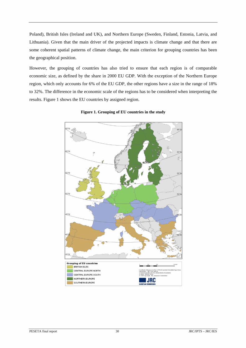
Lithuania). Given that the main driver of the projected impacts is climate change and that there are
some coherent spatial patterns of climate change, the main criterion for grouping countries has been
the geographical position.
However, the grouping of countries has also tried to ensure that each region is of comparable
economic size, as defined by the share in 2000 EU GDP. With the exception of the Northern Europe
region, which only accounts for 6% of the EU GDP, the other regions have a size in the range of 18%
to 32%. The difference in the economic scale of the regions has to be considered when interpreting the
results. Figure 1 shows the EU countries by assigned region.
Figure 1. Grouping of EU countries in the study
PESETA final report 30 JRC/IPTS – JRC/IES
2.3 Scenarios
The climate scenarios were selected to be useful for impact assessment modellers (e.g. Mearns et al.,
2003). Several criteria were considered: be based on state-of-the-art climate models and be
scientifically credible; be readily available; meet the data needs of the sectoral impact models; reflect
part of the range of the IPCC SRES emissions scenarios; and provide European-wide information at
high resolution for two future time periods: 2011-2040 and 2071-2100.
2.3.1 Socioeconomic scenarios
Underlying all climate scenarios are emissions and concentration scenarios, i.e. projections of
atmospheric concentrations of greenhouse gases and aerosols. The most widely-used scenarios come
from the Intergovernmental Panel on Climate Change (IPCC) Special Report on Emissions Scenarios
(SRES) (Nakicenovic and Swart, 2000). According to SRES and IPCC (2001; 2007a), none of the six
possible future storylines or the associated marker scenarios can be considered more likely than
another. However, it was not considered feasible within the constraints of the PESETA project to
consider more than two emissions scenarios. Thus two had to be chosen that were representative of the
full range, but also for which appropriate climate model output was available. For these reasons, it was
agreed to focus on the ‘high’ A2 scenario (which reaches a carbon dioxide concentration of 709 ppm
at 2100) together with the ‘low’ B2 scenario (which has a concentration of 560 ppm at 2100). Given
that the emissions are higher under the A2 scenario than in the B2 scenario, the consequences of the
A2 scenario could be interpreted as 'the cost of inaction'. However, as there are not explicit mitigation
policies in either scenario, that interpretation does not seem appropriate.
An overview of the main driving forces of the A2 and B2 scenarios is provided in Table 1. Global
population growth is much higher under the national enterprise A2 scenario, with population reaching
more than 15 billion by the end of the century, compared with 10.4 billion for the global stewardship
B2 scenario. This is obviously one of the main determinants of the lower emissions path of B2. GDP
expands in a similar way under the two scenarios. Moreover, the economic convergence of developing
countries is slower in A2. While the ratio of GDP per capita of developed to developing countries at
the end of the 21st century is four in the A2 scenario, it is only three under the B2 scenario.
PESETA final report 31 JRC/IPTS – JRC/IES
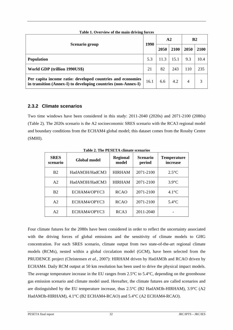
Table 1. Overview of the main driving forces
A2 B2 Scenario group 1990
2050 2100 2050 2100
Population 5.3 11.3 15.1 9.3 10.4
World GDP (trillion 1990US$) 21 82 243 110 235
Per capita income ratio: developed countries and economies in transition (Annex-I) to developing countries (non-Annex-I) 16.1 6.6 4.2 4 3
2.3.2 Climate scenarios
Two time windows have been considered in this study: 2011-2040 (2020s) and 2071-2100 (2080s)
(Table 2). The 2020s scenario is the A2 socioeconomic SRES scenario with the RCA3 regional model
and boundary conditions from the ECHAM4 global model; this dataset comes from the Rossby Centre
(SMHI).
Table 2. The PESETA climate scenarios
SRES scenario Global model Regional
model Scenario period
Temperature increase
B2 HadAM3H/HadCM3 HIRHAM 2071-2100 2.5°C
A2 HadAM3H/HadCM3 HIRHAM 2071-2100 3.9°C
B2 ECHAM4/OPYC3 RCAO 2071-2100 4.1°C
A2 ECHAM4/OPYC3 RCAO 2071-2100 5.4°C
A2 ECHAM4/OPYC3 RCA3 2011-2040 -
Four climate futures for the 2080s have been considered in order to reflect the uncertainty associated
with the driving forces of global emissions and the sensitivity of climate models to GHG
concentration. For each SRES scenario, climate output from two state-of-the-art regional climate
models (RCMs), nested within a global circulation model (GCM), have been selected from the
PRUDENCE project (Christensen et al., 2007): HIRHAM driven by HadAM3h and RCAO driven by
ECHAM4. Daily RCM output at 50 km resolution has been used to drive the physical impact models.
The average temperature increase in the EU ranges from 2.5°C to 5.4°C, depending on the greenhouse
gas emission scenario and climate model used. Hereafter, the climate futures are called scenarios and
are distinguished by the EU temperature increase, thus 2.5°C (B2 HadAM3h-HIRHAM), 3.9°C (A2
HadAM3h-HIRHAM), 4.1°C (B2 ECHAM4-RCAO) and 5.4°C (A2 ECHAM4-RCAO).
PESETA final report 32 JRC/IPTS – JRC/IES
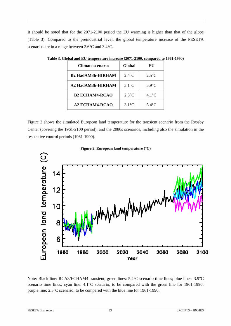
It should be noted that for the 2071-2100 period the EU warming is higher than that of the globe
(Table 3). Compared to the preindustrial level, the global temperature increase of the PESETA
scenarios are in a range between 2.6°C and 3.4°C.
Table 3. Global and EU temperature increase (2071-2100, compared to 1961-1990)
Climate scenario Global EU
B2 HadAM3h-HIRHAM 2.4°C 2.5°C
A2 HadAM3h-HIRHAM 3.1°C 3.9°C
B2 ECHAM4-RCAO 2.3°C 4.1°C
A2 ECHAM4-RCAO 3.1°C 5.4°C
Figure 2 shows the simulated European land temperature for the transient scenario from the Rossby
Center (covering the 1961-2100 period), and the 2080s scenarios, including also the simulation in the
respective control periods (1961-1990).
Figure 2. European land temperature (°C)
Note: Black line: RCA3/ECHAM4 transient; green lines: 5.4°C scenario time lines; blue lines: 3.9°C scenario time lines; cyan line: 4.1°C scenario; to be compared with the green line for 1961-1990; purple line: 2.5°C scenario; to be compared with the blue line for 1961-1990.
PESETA final report 33 JRC/IPTS – JRC/IES
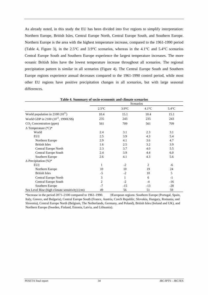
As already noted, in this study the EU has been divided into five regions to simplify interpretation:
Northern Europe, British Isles, Central Europe North, Central Europe South, and Southern Europe.
Northern Europe is the area with the highest temperature increase, compared to the 1961-1990 period
(Table 4, Figure 3), in the 2.5°C and 3.9°C scenarios, whereas in the 4.1°C and 5.4°C scenarios
Central Europe South and Southern Europe experience the largest temperature increases. The more
oceanic British Isles have the lowest temperature increase throughout all scenarios. The regional
precipitation pattern is similar in all scenarios (Figure 4). The Central Europe South and Southern
Europe regions experience annual decreases compared to the 1961-1990 control period, while most
other EU regions have positive precipitation changes in all scenarios, but with large seasonal
differences.
Table 4. Summary of socio-economic and climate scenarios
2.5°C 3.9°C 4.1°C 5.4°C
World population in 2100 (1012) 10.4 15.1 10.4 15.1World GDP in 2100 (1012, 1990US$) 235 243 235 243CO2 Concentration (ppm) 561 709 561 709Δ Temperature (ºC)*
World 2.4 3.1 2.3 3.1EU‡ 2.5 3.9 4.3 5.4 Northern Europe 2.9 4.1 3.6 4.7 British Isles 1.6 2.5 3.2 3.9 Central Europe North 2.3 3.7 4.0 5.5 Central Europe South 2.4 3.9 4.4 6.0 Southern Europe 2.6 4.1 4.3 5.6
Δ Precipitation (%)*EU‡ 1 -2 2 -6 Northern Europe 10 10 19 24 British Isles -5 -2 10 5 Central Europe North 3 1 6 -1 Central Europe South 2 -2 -4 -16 Southern Europe -7 -15 -13 -28
Sea Level Rise (high climate sensitivity) (cm) 49 56 51 59
Scenarios
*Increase in the period 2071–2100 compared to 1961–1990. ‡European regions: Southern Europe (Portugal, Spain, Italy, Greece, and Bulgaria), Central Europe South (France, Austria, Czech Republic, Slovakia, Hungary, Romania, and Slovenia), Central Europe North (Belgium, The Netherlands, Germany, and Poland), British Isles (Ireland and UK), and Northern Europe (Sweden, Finland, Estonia, Latvia, and Lithuania).
PESETA final report 34 JRC/IPTS – JRC/IES
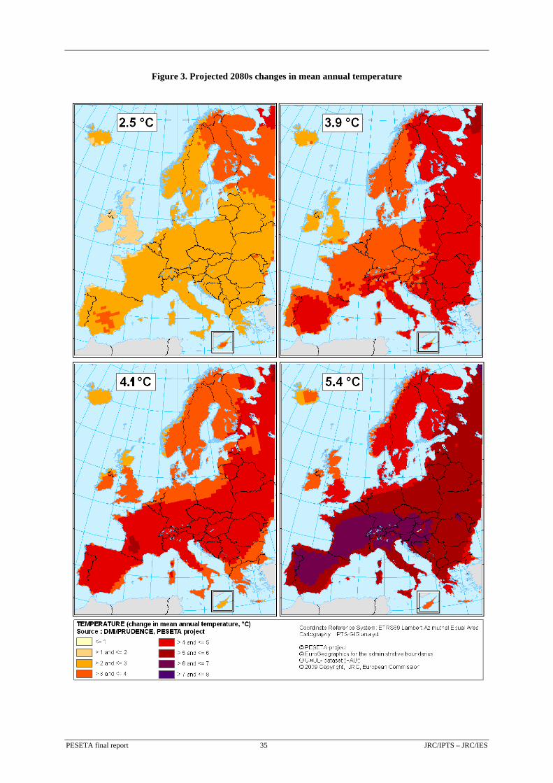
Figure 3. Projected 2080s changes in mean annual temperature
PESETA final report 35 JRC/IPTS – JRC/IES
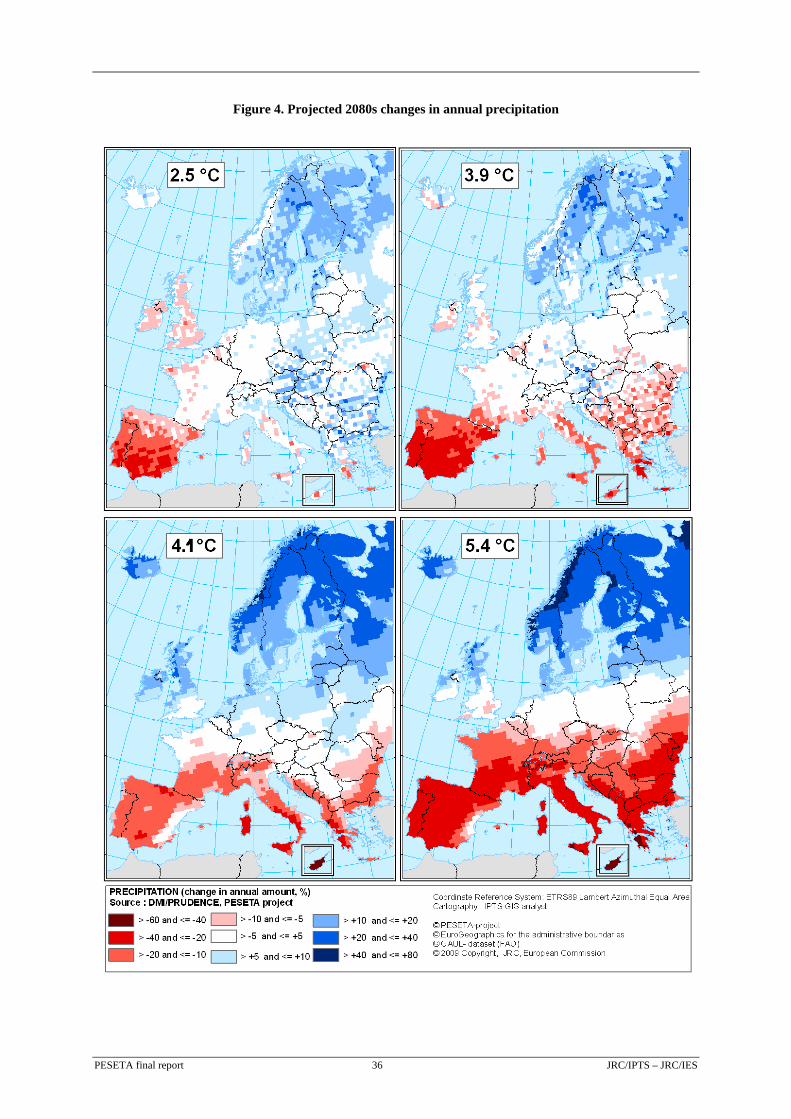
Figure 4. Projected 2080s changes in annual precipitation
PESETA final report 36 JRC/IPTS – JRC/IES
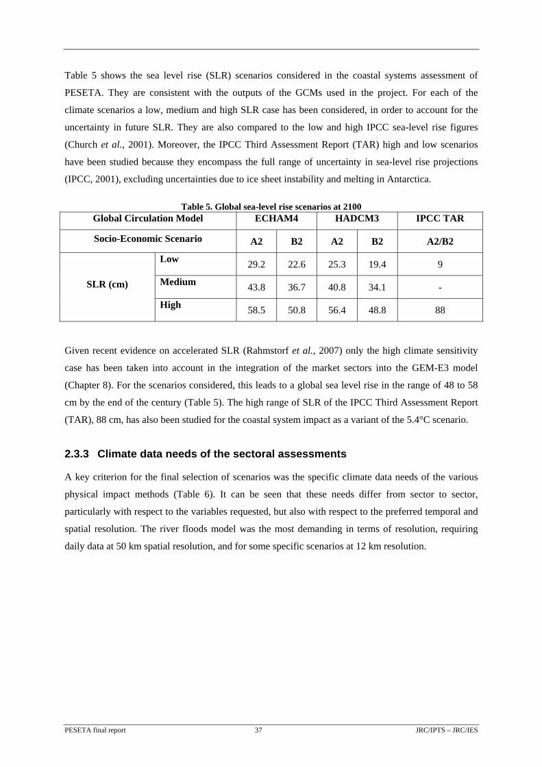
Table 5 shows the sea level rise (SLR) scenarios considered in the coastal systems assessment of
PESETA. They are consistent with the outputs of the GCMs used in the project. For each of the
climate scenarios a low, medium and high SLR case has been considered, in order to account for the
uncertainty in future SLR. They are also compared to the low and high IPCC sea-level rise figures
(Church et al., 2001). Moreover, the IPCC Third Assessment Report (TAR) high and low scenarios
have been studied because they encompass the full range of uncertainty in sea-level rise projections
(IPCC, 2001), excluding uncertainties due to ice sheet instability and melting in Antarctica.
Table 5. Global sea-level rise scenarios at 2100 Global Circulation Model ECHAM4 HADCM3 IPCC TAR
Socio-Economic Scenario A2 B2 A2 B2 A2/B2
Low 29.2 22.6 25.3 19.4 9
Medium 43.8 36.7 40.8 34.1 - SLR (cm)
High 58.5 50.8 56.4 48.8 88
Given recent evidence on accelerated SLR (Rahmstorf et al., 2007) only the high climate sensitivity
case has been taken into account in the integration of the market sectors into the GEM-E3 model
(Chapter 8). For the scenarios considered, this leads to a global sea level rise in the range of 48 to 58
cm by the end of the century (Table 5). The high range of SLR of the IPCC Third Assessment Report
(TAR), 88 cm, has also been studied for the coastal system impact as a variant of the 5.4°C scenario.
2.3.3 Climate data needs of the sectoral assessments
A key criterion for the final selection of scenarios was the specific climate data needs of the various
physical impact methods (Table 6). It can be seen that these needs differ from sector to sector,
particularly with respect to the variables requested, but also with respect to the preferred temporal and
spatial resolution. The river floods model was the most demanding in terms of resolution, requiring
daily data at 50 km spatial resolution, and for some specific scenarios at 12 km resolution.
PESETA final report 37 JRC/IPTS – JRC/IES
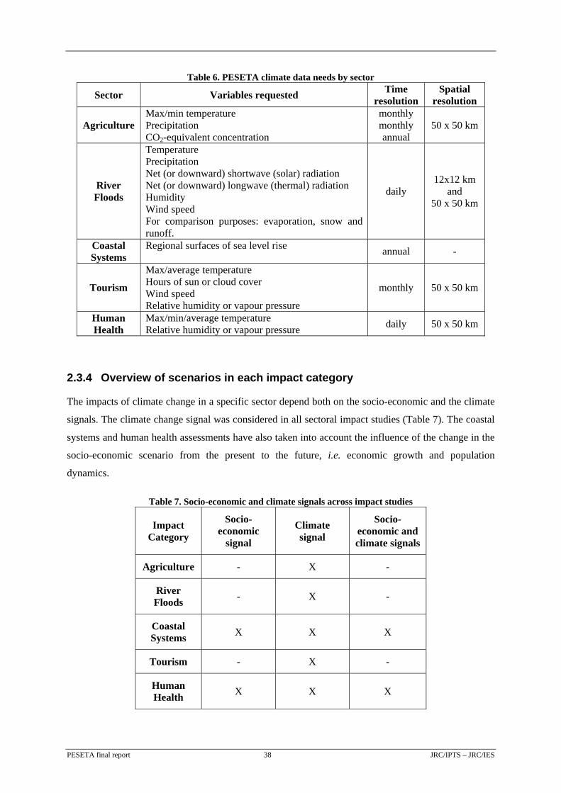
Table 6. PESETA climate data needs by sector
Sector Variables requested Time resolution
Spatial resolution
Agriculture Max/min temperature Precipitation CO2-equivalent concentration
monthly monthly annual
50 x 50 km
River Floods
Temperature Precipitation Net (or downward) shortwave (solar) radiation Net (or downward) longwave (thermal) radiation Humidity Wind speed For comparison purposes: evaporation, snow and runoff.
daily 12x12 km
and 50 x 50 km
Coastal Systems
Regional surfaces of sea level rise annual -
Tourism
Max/average temperature Hours of sun or cloud cover Wind speed Relative humidity or vapour pressure
monthly 50 x 50 km
Human Health
Max/min/average temperature Relative humidity or vapour pressure daily 50 x 50 km
2.3.4 Overview of scenarios in each impact category
The impacts of climate change in a specific sector depend both on the socio-economic and the climate
signals. The climate change signal was considered in all sectoral impact studies (Table 7). The coastal
systems and human health assessments have also taken into account the influence of the change in the
socio-economic scenario from the present to the future, i.e. economic growth and population
dynamics.
Table 7. Socio-economic and climate signals across impact studies
Impact Category
Socio-economic
signal
Climate signal
Socio-economic and climate signals
Agriculture - X -
River Floods - X -
Coastal Systems X X X
Tourism - X -
Human Health X X X
PESETA final report 38 JRC/IPTS – JRC/IES
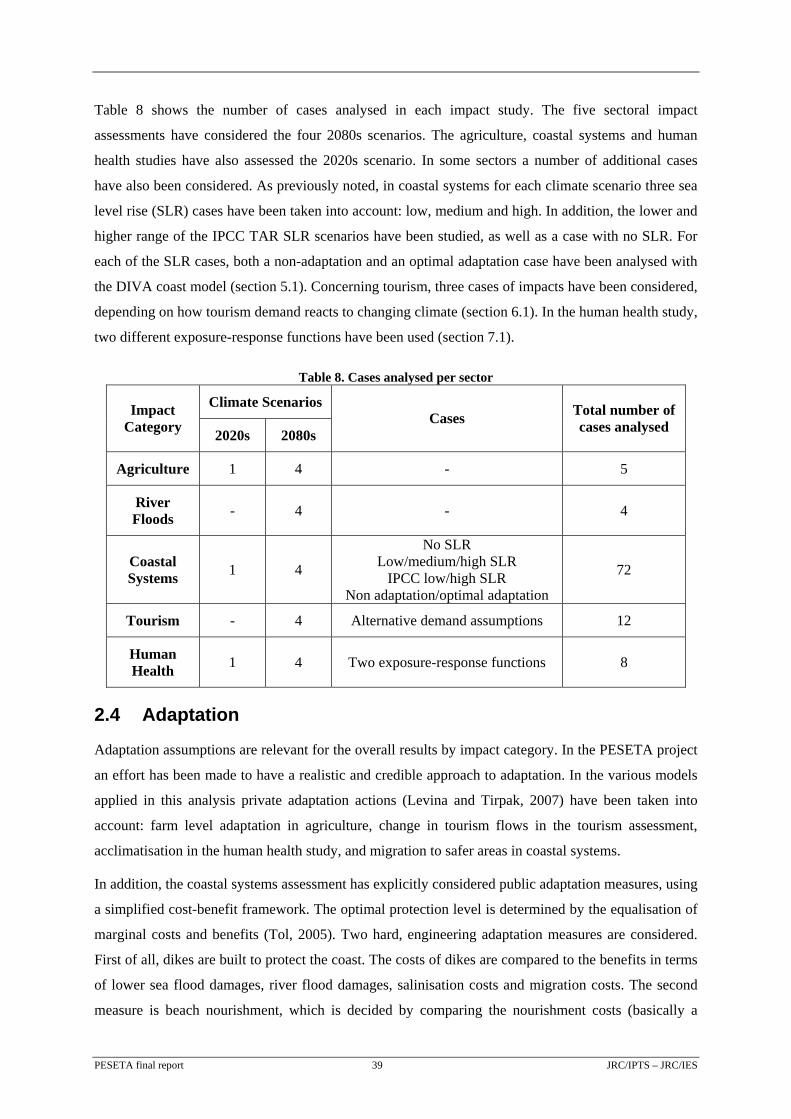
Table 8 shows the number of cases analysed in each impact study. The five sectoral impact
assessments have considered the four 2080s scenarios. The agriculture, coastal systems and human
health studies have also assessed the 2020s scenario. In some sectors a number of additional cases
have also been considered. As previously noted, in coastal systems for each climate scenario three sea
level rise (SLR) cases have been taken into account: low, medium and high. In addition, the lower and
higher range of the IPCC TAR SLR scenarios have been studied, as well as a case with no SLR. For
each of the SLR cases, both a non-adaptation and an optimal adaptation case have been analysed with
the DIVA coast model (section 5.1). Concerning tourism, three cases of impacts have been considered,
depending on how tourism demand reacts to changing climate (section 6.1). In the human health study,
two different exposure-response functions have been used (section 7.1).
Table 8. Cases analysed per sector
Climate Scenarios Impact Category 2020s 2080s
Cases Total number of cases analysed
Agriculture 1 4 - 5
River Floods - 4 - 4
Coastal Systems 1 4
No SLR Low/medium/high SLR
IPCC low/high SLR Non adaptation/optimal adaptation
72
Tourism - 4 Alternative demand assumptions 12
Human Health 1 4 Two exposure-response functions 8
2.4 Adaptation
Adaptation assumptions are relevant for the overall results by impact category. In the PESETA project
an effort has been made to have a realistic and credible approach to adaptation. In the various models
applied in this analysis private adaptation actions (Levina and Tirpak, 2007) have been taken into
account: farm level adaptation in agriculture, change in tourism flows in the tourism assessment,
acclimatisation in the human health study, and migration to safer areas in coastal systems.
In addition, the coastal systems assessment has explicitly considered public adaptation measures, using
a simplified cost-benefit framework. The optimal protection level is determined by the equalisation of
marginal costs and benefits (Tol, 2005). Two hard, engineering adaptation measures are considered.
First of all, dikes are built to protect the coast. The costs of dikes are compared to the benefits in terms
of lower sea flood damages, river flood damages, salinisation costs and migration costs. The second
measure is beach nourishment, which is decided by comparing the nourishment costs (basically a
PESETA final report 39 JRC/IPTS – JRC/IES
function of cubic metre of sand) with its benefits. The benefits depend on agriculture land value if
there are not tourists, and where there are tourists, the benefits depend on the number of tourists and
their expenditure.
2.5 Economic assessment
2.5.1 Discounting
The simulated economic effects of climate change refer to the 2020s and 2080s. Yet those effects
cannot be directly compared to the size of the economy as of today. Economic effects are usually
discounted in order to account both for the growth in per capita income of the economy (the same
Euro has a higher value today than for the richer future society) and the fact that there is a preference
for current consumption versus future consumption (as reflected in the positive interest rate e.g. of
public bonds).
However the choice of the discount rate is a very controversial issue (Stern and Taylor, 2007;
Nordhaus, 2007) because it requires value judgements, e.g. the valuation of future generations' welfare
by today's generation.
In order to make the economic assessment of PESETA transparent it was decided to report
undiscounted monetary effects in the economic estimates for the 2080s. Concerning the integration of
market impacts into the GEM-E3 model (Chapter 8), as the evaluation is made concerning the impacts
of future climate on today's economy, so discounting monetary impacts is not required.
2.5.2 Valuation methods: direct economic effects
The sectoral studies produced estimates of the "direct" economic effect. Those effects are limited to
the sector under consideration and do not take into account the consequences in the rest of the
economy. This is known in the economic literature as partial equilibrium analysis.
The river flood, coastal systems, tourism and human health studies have made a direct economic effect
analysis. In particular, the river flood assessment considers the direct damages due to river floods,
mainly affecting residential buildings and economic activities (Section 4.3). The costal systems study
considers the impacts in terms of land losses, migration costs and sea flood costs (Section 5.3). The
tourism study measures the effect in tourism expenditure from assumptions on expenditure per bed
night (Section 6.3). Finally, the human health study values mortality effects using standard economic
methods: value of statistical life and value of life years lost (Section 7.3).
Nevertheless, the direct effects provide only part of the overall economic consequences of climate
change because they will also affect the rest of the economy (e.g. Darwin and Tol, 2001). This is the
case for instance of river floods. The impact assessment provides the damages due to land uses in the
PESETA final report 40 JRC/IPTS – JRC/IES
PESETA final report 41 JRC/IPTS – JRC/IES
flooded area. But those damages also will induce additional effects in other sectors and aspects of the
economy. Thus the damages to the commercial sector will lead to lower income for the business
owners, which will lead to lower expenditure by them, additionally depressing economic activity in
other sectors of the economy. A similar case occurs with agriculture. In countries facing drops in
yields, other industries will undergo lower production levels, such as the agroindustry sector. The
study of the overall economic consequences, considering the indirect effects in addition to the direct
effects, can be made with computable general equilibrium (CGE) models (Shoven and Whalley,
1992).
2.5.3 Valuation methods: overall economic (general equilibrium) effects
Two sectoral studies have applied the CGE methodology. The agriculture and coastal system
assessments have both used the GTAP general equilibrium model to value the overall effects on the
economy. They have assessed the impact of future climate on the future economy. Both the climate
signal and socioeconomic change have been taken into account.
Moreover, in the last stage of the project the four impact categories that can be considered as 'market'
impacts (agriculture, river floods, coastal systems and tourism) have been integrated in the GEM-E3
CGE model (Chapter 8). There, to ensure consistency, only the impact due to climate change is
considered, which was studied in all sectors (Table 7).

3 AGRICULTURE IMPACT ASSESSMENT
Agriculture is the main user of land, and water, and it still defines society in the rural areas of Europe.
European agriculture accounts for one half of the global trade of food products and it is directly
influenced by European and global policy. Climatic conditions directly affect agriculture and the water
resources needed to maintain a stable production in many areas of Europe (Iglesias et al., 2007; 2009a;
Olesen and Bindi, 2002) and the provision of essential ecosystem services (Metzger et al., 2006). It is
likely that the stress imposed by climate change on agriculture and water intensifies the regional
disparities in rural areas and the overall economy of European countries (Alcamo et al., 2007; EEA,
2008; Stern, 2007). Understanding the impact of climate change is complicated because changes in
physical and social variables are often derived by using different assumptions and inconsistency of
inputs across geographical and time scales. As a result, some of the most profound impacts of climate
change may be more difficult to project than the future climate itself.
This chapter summarises the methodology and the main results of the agriculture impact assessment.
Detailed information can be found in the accompanying PESETA technical report of Iglesias et al.
(2009b).
3.1 Agriculture integrated methodology
3.1.1 The modelling approach
European scenarios of agricultural change for the years 2020s and 2080s are developed based on
global scenarios of changes in environmental and socio-economic variables and the understanding of
the sensitivity of each agricultural region to these changes. The most important determinants of
changes in agricultural production are: changes in agroclimatic regions, crop productivity, and crop
management (deliberate adjustments of the crop calendar, nitrogen fertiliser, and amount of irrigation
water in order to optimise productivity in each scenario); livestock production is not considered,
except for the possible inference of crop productivity. Then, the expected change in future crop
productivity is calculated across Europe. Finally, monetary estimates of the projected changes are
derived. It is assumed that (i) farmers follow an adjusted crop management in response to climate; (ii)
irrigated areas do not increase significantly; and (iii) fiscal policies remain unchanged. Because of the
nature of these assumptions, it is considered that the results represent an agricultural policy scenario
that does not impose major additional environmental restrictions beyond the ones currently
implemented, neither include pollution taxes (for example for nitrogen emissions to mitigate climate
change).
The assessment links biophysical and statistical models in a rigorous and testable methodology, based
on current understanding of processes of crop growth and development, to quantify crop responses to
PESETA final report 43 JRC/IPTS – JRC/IES
changing climate conditions. Dynamic process-based crop growth models are specified and validated
for sites in the major agro-climatic regions of Europe. The validated site crop models are useful for
simulating the range of conditions under which crops are grown, and provide the means to estimate
production functions when experimental field data are not available. Variables explaining a significant
proportion of simulated yield variance are crop water (sum of precipitation and irrigation) and
temperature over the growing season. Crop production functions are derived from the process based
model results. The functional forms for each region represent the realistic water limited and potential
conditions for the mix of crops, management alternatives, and potential endogenous adaptation to
climate assumed in each area.
In particular, nine agro-climatic regions are defined based on K-mean cluster analysis of temperature
and precipitation data from 247 meteorological stations, district crop yield data, and irrigation data.
The yield functions derived from the validated crop model, the DSSAT model (Rosenzweig and
Iglesias, 2008; Rosenzweig and Iglesias, 2002; Iglesias et al., 2006; Rosenzweig and Iglesias, 1994),
are then used with the spatial agro-climatic database to conduct a European wide spatial analysis of
crop production vulnerability to climate change.
Adaptation is explicitly considered and incorporated into the results by assessing country or regional
potential for reaching optimal crop yield. Optimal yield is the potential yield given non-limiting water
applications, fertilizer inputs, and management constraints. Adapted yields are calculated in each
country or region as a fraction of the potential yield. That fraction is determined by the ratio of current
yields to current yield potential.
The methodology incorporates a number of strengths: it is based on an interdisciplinary, consistent
bottom-up methodology that uses a range of emission scenarios to provide insights into the effects of
climate change policy. The physical approach expands process-based crop model results over large
areas and therefore overcomes the limitation of data requirements for the crop models; it includes
conditions that are beyond the range of historical observations of crop yield data; and includes
simulation of optimal management and thus estimate agricultural responses to changes in regional
climate.
3.1.2 Limitations and uncertainties
There is a large uncertainty surrounding future emissions and their underlying dynamic driving forces.
This uncertainty is increased in going from emission values to climate change, from climate change to
possible impacts and finally from these driving forces to formulating adaptation and mitigation
policies (Gupta et al., 2003). The study considers changes in agroclimatic regions but not on the
evolution of land use to the 2080s. Determining how farmers will adapt to climate change is a very
complex dynamic process which is difficult to quantify. The study considers that farmers optimise
PESETA final report 44 JRC/IPTS – JRC/IES
management under climate change scenarios but cannot implement changes that require policy
intervention. How agriculture policies might react to a changing climate is another critical factor
which cannot be incorporated in the simulations.
The uncertainty of the climate scenario is characterised by selecting two emission scenarios (A2 and
B2), two global climate models (HadCM3 and ECHAM) downscaled across Europe, and two time
frames. In all regions, uncertainties with respect to the magnitude of the expected climate changes
result in uncertainties of the agricultural evaluations. For example, in some regions projections of
rainfall, a key variable for crop production may be positive or negative depending on the climate
scenario used and variable in each season. In general, the assessment shows that the estimated yield
changes vary more among different climate models, while the GDP projections show more
discrepancy across socio-economic scenarios. Nevertheless, the time horizon is the main determinant
of the physical and economic projections.
3.2 Physical impacts
The results show that agroclimatic regions will have substantial modifications as a result of climate
change, in agreement to previous analyses. These changes in agroclimatic regions have important
implications for the evaluation of impacts on future crop productivity. Here, the production functions
are implemented in future agroclimatic regions - that is, the farmers in each location in the future have
knowledge of how and what to produce. That is, the crop productivity changes include the changes in
crop distribution in the scenario due to modified crop suitability under the warmer climate and
farmers’ adaptation (non-policy driven). European crop yield changes include the direct positive
effects of CO2 on the crops, the rain-fed and irrigated simulations in each district. It is very important
to notice that the simulations considered no restrictions in water availability for irrigation due to
changes in policy. In all cases, the simulations did not include restrictions in the application of
nitrogen fertilizer. Therefore the results should be considered optimistic from the production point and
pessimistic from the environmental point of view.
There are large differences among European regions in the impacts of global change in crop
productivity. Figure 5 to Figure 8 shows modelled European crop yield changes for all the 2080s
scenarios, and Figure 9 for the 2020s scenario. The estimates for each European region appear in
Table 1. The crop productivity changes include the changes in crop distribution in the scenario due to
modified crop suitability under the warmer climate and farmers’ adaptation. The 2080s less warming
scenarios would lead to small changes in yields for the EU, while the 5.4°C scenario could mean a fall
in crop yields of 10%. All 2080s scenarios share a similar pattern in the spatial distribution of effects.
High yield improvements in Northern Europe are caused by lengthened growing season, which
decreases cold effects on growth and extends the frost-free period. Crop productivity decreases in
Southern Europe are caused by a shortening of the growing period, with subsequent negative effects
PESETA final report 45 JRC/IPTS – JRC/IES
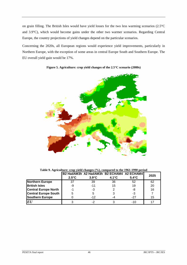
PESETA final report 46 JRC/IPTS – JRC/IES
on grain filling. The British Isles would have yield losses for the two less warming scenarios (2.5°C
and 3.9°C), which would become gains under the other two warmer scenarios. Regarding Central
Europe, the country projections of yield changes depend on the particular scenarios.
Concerning the 2020s, all European regions would experience yield improvements, particularly in
Northern Europe, with the exception of some areas in central Europe South and Southern Europe. The
EU overall yield gain would be 17%.
Figure 5. Agriculture: crop yield changes of the 2.5°C scenario (2080s)
Table 9. Agriculture: crop yield changes (%), compared to the 1961-1990 period B2 HadAM3h A2 HadAM3h B2 ECHAM4 A2 ECHAM4
2.5°C 3.9°C 4.1°C 5.4°CNorthern Europe 37 39 36 52 62British Isles -9 -11 15 19 20Central Europe North -1 -3 2 -8 16Central Europe South 5 5 3 -3Southern Europe 0 -12 -4 -27 15EU 3 -2 3 -10 1
2025
7
7
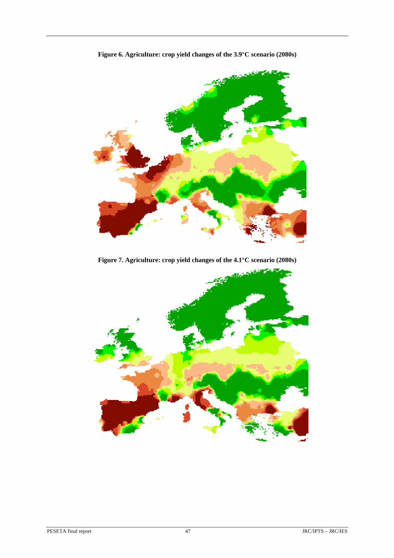
Figure 6. Agriculture: crop yield changes of the 3.9°C scenario (2080s)
Figure 7. Agriculture: crop yield changes of the 4.1°C scenario (2080s)
PESETA final report 47 JRC/IPTS – JRC/IES
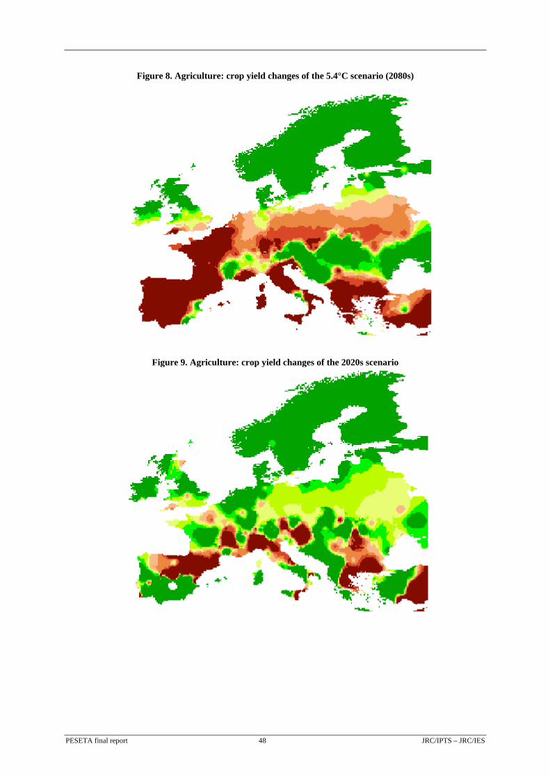
Figure 8. Agriculture: crop yield changes of the 5.4°C scenario (2080s)
Figure 9. Agriculture: crop yield changes of the 2020s scenario
PESETA final report 48 JRC/IPTS – JRC/IES
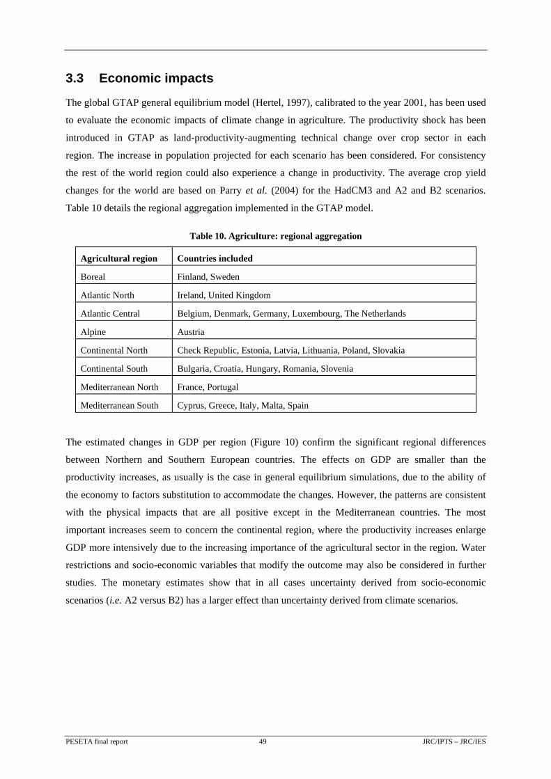
3.3 Economic impacts
The global GTAP general equilibrium model (Hertel, 1997), calibrated to the year 2001, has been used
to evaluate the economic impacts of climate change in agriculture. The productivity shock has been
introduced in GTAP as land-productivity-augmenting technical change over crop sector in each
region. The increase in population projected for each scenario has been considered. For consistency
the rest of the world region could also experience a change in productivity. The average crop yield
changes for the world are based on Parry et al. (2004) for the HadCM3 and A2 and B2 scenarios.
Table 10 details the regional aggregation implemented in the GTAP model.
Table 10. Agriculture: regional aggregation
Agricultural region Countries included
Boreal Finland, Sweden
Atlantic North Ireland, United Kingdom
Atlantic Central Belgium, Denmark, Germany, Luxembourg, The Netherlands
Alpine Austria
Continental North Check Republic, Estonia, Latvia, Lithuania, Poland, Slovakia
Continental South Bulgaria, Croatia, Hungary, Romania, Slovenia
Mediterranean North France, Portugal
Mediterranean South Cyprus, Greece, Italy, Malta, Spain
The estimated changes in GDP per region (Figure 10) confirm the significant regional differences
between Northern and Southern European countries. The effects on GDP are smaller than the
productivity increases, as usually is the case in general equilibrium simulations, due to the ability of
the economy to factors substitution to accommodate the changes. However, the patterns are consistent
with the physical impacts that are all positive except in the Mediterranean countries. The most
important increases seem to concern the continental region, where the productivity increases enlarge
GDP more intensively due to the increasing importance of the agricultural sector in the region. Water
restrictions and socio-economic variables that modify the outcome may also be considered in further
studies. The monetary estimates show that in all cases uncertainty derived from socio-economic
scenarios (i.e. A2 versus B2) has a larger effect than uncertainty derived from climate scenarios.
PESETA final report 49 JRC/IPTS – JRC/IES
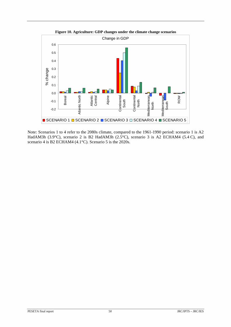
Figure 10. Agriculture: GDP changes under the climate change scenarios
Change in GDP
-0.2
-0.1
0.0
0.1
0.2
0.3
0.4
0.5
0.6
Bor
eal
Atla
ntic
Nor
th
Atla
ntic
Cen
tral
Alp
ine
Con
tinen
tal
Sou
th
Con
tinen
tal
Nor
th
Med
iterra
nean
Nor
th
Med
iterra
nean
Sou
th RO
W
% c
hang
e
SCENARIO 1 SCENARIO 2 SCENARIO 3 SCENARIO 4 SCENARIO 5
Note: Scenarios 1 to 4 refer to the 2080s climate, compared to the 1961-1990 period: scenario 1 is A2 HadAM3h (3.9°C), scenario 2 is B2 HadAM3h (2.5°C), scenario 3 is A2 ECHAM4 (5.4 C), and scenario 4 is B2 ECHAM4 (4.1°C). Scenario 5 is the 2020s.
PESETA final report 50 JRC/IPTS – JRC/IES
4 RIVER FLOODS ASSESSMENT
River floods are the most common natural disaster in Europe (EEA, 2004). Global warming is
generally expected to increase the magnitude and frequency of extreme precipitation events
(Christensen and Christensen, 2003; Frei et al., 2006), which may lead to more intense and frequent
river floods.
This chapter summarises the methodology and the main results of the river flood impact assessment.
Detailed information on the methodology can be found in Feyen et al. (2006).
4.1 Modelling floods in river basins
4.1.1 The modelling approach
Estimates of changes in the frequency and severity of river floods are based on simulations with the
LISFLOOD model followed by extreme value analysis (Dankers and Feyen, 2008). The LISFLOOD
model, which transfers the climate forcing data (temperature, precipitation, radiation, wind-speed,
humidity) into river runoff estimates, is a spatially distributed, mixed conceptual-physically based
hydrological model developed for flood forecasting and impact assessment studies at the European
scale (van der Knijff et al., 2008). Using a planar approximation approach, the simulated discharges
with return periods of 2, 5, 10, 20, 50, 100, 250 and 500 years have been converted into flood
inundation extents and depths. The latter have been translated into direct monetary damage from
contact with floodwaters using country specific flood depth-damage functions (Huizinga, 2007) and
land use information (EEA, 2000). Population exposure has been assessed by overlaying the flood
inundation information with data on population density (Gallego and Peedell, 2001). By linearly
interpolating damages and population exposed between the different return periods, damage and
population exposure probability functions have been constructed under present and future climate.
From the latter, the expected annual damage and expected annual population exposed have been
calculated.
Static, country-specific protective capacities for floods have been considered by truncating the damage
and population exposure probability functions at certain return periods. Various flood protection levels
were imposed depending on country GDP per capita (protection to 100-year, 75-year and 50-year
return periods).
It is assumed that the population and the economic structure are as of today's. Therefore, the additional
damage that would occur because of population growth and economic development has not been
considered in this assessment. In this respect, the figures below underestimate the projected damages
by the end of the century.
PESETA final report 51 JRC/IPTS – JRC/IES
4.1.2 Limitations and uncertainties
The different steps in the chain “emissions → climate → extreme flow → flood inundation →
damage” are subject to uncertainty. When applying the framework outlined above for macro-scale
flood damage assessment it was necessary to adopt a series of assumptions, which should be kept in
mind when interpreting the results. First of all, the climate scenarios used only capture a part of the
uncertainty range attributable to emissions of greenhouse gasses (with the A2 and B2 scenarios only
two out of six SRES storylines are considered) and neglect uncertainty due to inter-GCM and inter-
RCM variability. Secondly, no downscaling or bias correction was applied to the climate data because
at present no high-quality, high-resolution meteorological dataset exists at European scale that would
allow a proper downscaling of the climate data used. This may locally lead to underestimation of flood
frequencies due to the inability of the RCM to explicitly represent fine-scale climatic structures,
especially for the coarse resolution run (B2, 50 km). Thirdly, hydrological uncertainty is not accounted
for. Several studies (e.g., Wilby, 2005) showed, however, that this layer of uncertainty is generally
much lower than the uncertainty of the climate input to the hydrological model. Fourthly, flood return
levels are estimated using extreme value analysis based on simulated time series of 30 years, which
may result in large extrapolation errors for high return periods. Moreover, changes in land use and
land cover are not incorporated in the climate runs or in the economic impact evaluation due to the
absence of reasonable macro-scale land use change scenarios for the SRES storylines. This may result
in an underestimation of future flood risk.
The approach used is based on direct estimated potential flood damage caused by water depths on land
use typologies. Other factors that might contribute to the increase of losses, such as flood velocity,
building characteristics, content of sediment in water, as well as indirect economic losses, are not
included in this study.
The above list of assumptions implies that monetary estimates of flood damage are inherently
uncertain. It should be noted, however, that the goal of this study was to evaluate changes in flood
damage due to climate change, rather than to estimate absolute values of flood damage. Given that
most of the assumptions apply to both the control and scenario period it can be expected that estimates
of changes in flood damage are relatively less affected by the assumptions compared to the absolute
flood damage estimates.
4.2 Physical impacts
Figure 11 shows the change in the 100-year return level of river discharge between the scenario and
control run for the 3.9°C and 2.5°C scenarios. Note that an increase or decrease in the 100-year return
discharge translates as an increase or decrease in the probability of occurrence of a current 100-year
PESETA final report 52 JRC/IPTS – JRC/IES
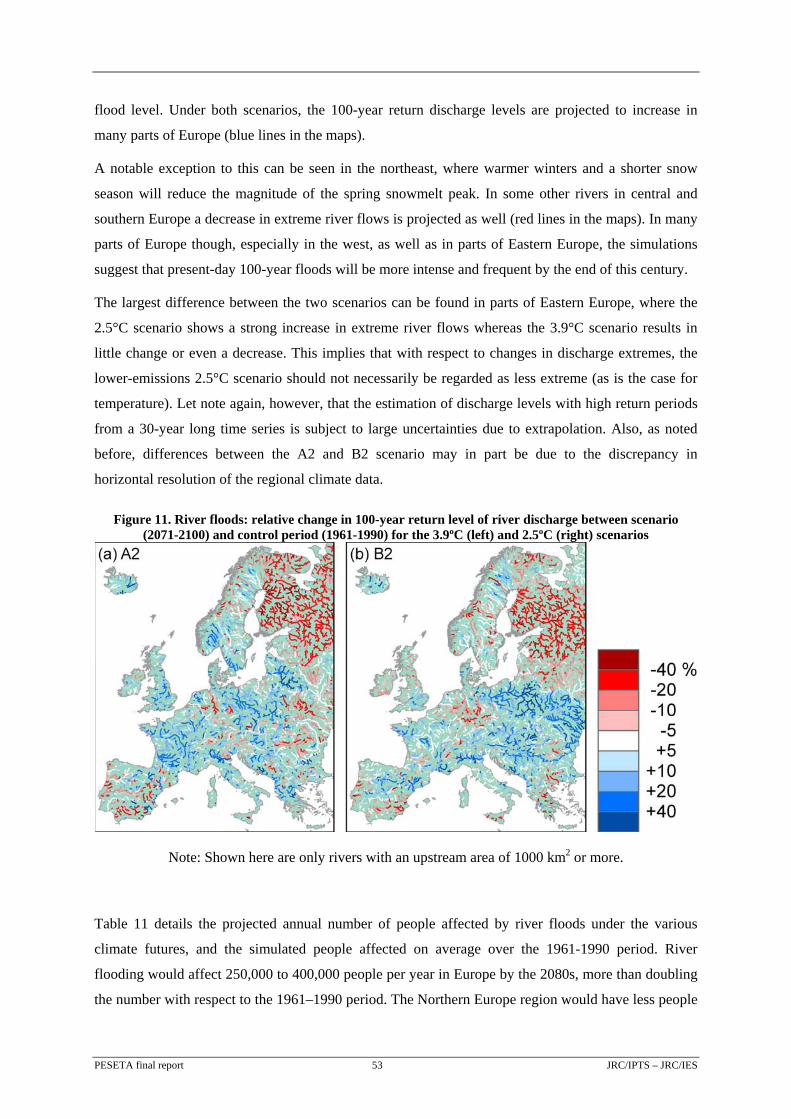
flood level. Under both scenarios, the 100-year return discharge levels are projected to increase in
many parts of Europe (blue lines in the maps).
A notable exception to this can be seen in the northeast, where warmer winters and a shorter snow
season will reduce the magnitude of the spring snowmelt peak. In some other rivers in central and
southern Europe a decrease in extreme river flows is projected as well (red lines in the maps). In many
parts of Europe though, especially in the west, as well as in parts of Eastern Europe, the simulations
suggest that present-day 100-year floods will be more intense and frequent by the end of this century.
The largest difference between the two scenarios can be found in parts of Eastern Europe, where the
2.5°C scenario shows a strong increase in extreme river flows whereas the 3.9°C scenario results in
little change or even a decrease. This implies that with respect to changes in discharge extremes, the
lower-emissions 2.5°C scenario should not necessarily be regarded as less extreme (as is the case for
temperature). Let note again, however, that the estimation of discharge levels with high return periods
from a 30-year long time series is subject to large uncertainties due to extrapolation. Also, as noted
before, differences between the A2 and B2 scenario may in part be due to the discrepancy in
horizontal resolution of the regional climate data.
Figure 11. River floods: relative change in 100-year return level of river discharge between scenario (2071-2100) and control period (1961-1990) for the 3.9ºC (left) and 2.5ºC (right) scenarios
Note: Shown here are only rivers with an upstream area of 1000 km2 or more.
Table 11 details the projected annual number of people affected by river floods under the various
climate futures, and the simulated people affected on average over the 1961-1990 period. River
flooding would affect 250,000 to 400,000 people per year in Europe by the 2080s, more than doubling
the number with respect to the 1961–1990 period. The Northern Europe region would have less people
PESETA final report 53 JRC/IPTS – JRC/IES
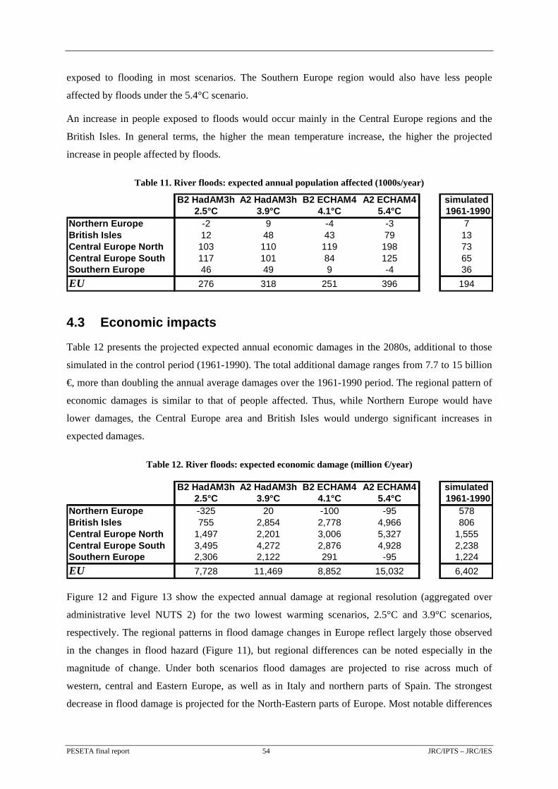
exposed to flooding in most scenarios. The Southern Europe region would also have less people
affected by floods under the 5.4°C scenario.
An increase in people exposed to floods would occur mainly in the Central Europe regions and the
British Isles. In general terms, the higher the mean temperature increase, the higher the projected
increase in people affected by floods.
Table 11. River floods: expected annual population affected (1000s/year)
B2 HadAM3h A2 HadAM3h B2 ECHAM4 A2 ECHAM4 simulated2.5°C 3.9°C 4.1°C 5.4°C 1961-1990
Northern Europe -2 9 -4 -3 7British Isles 12 48 43 79 13Central Europe North 103 110 119 198 73Central Europe South 117 101 84 125 65Southern Europe 46 49 9 -4 36EU 276 318 251 396 194
4.3 Economic impacts
Table 12 presents the projected expected annual economic damages in the 2080s, additional to those
simulated in the control period (1961-1990). The total additional damage ranges from 7.7 to 15 billion
€, more than doubling the annual average damages over the 1961-1990 period. The regional pattern of
economic damages is similar to that of people affected. Thus, while Northern Europe would have
lower damages, the Central Europe area and British Isles would undergo significant increases in
expected damages.
Table 12. River floods: expected economic damage (million €/year)
B2 HadAM3h A2 HadAM3h B2 ECHAM4 A2 ECHAM4 simulated2.5°C 3.9°C 4.1°C 5.4°C 1961-1990
Northern Europe -325 20 -100 -95 578British Isles 755 2,854 2,778 4,966 806Central Europe North 1,497 2,201 3,006 5,327 1,555Central Europe South 3,495 4,272 2,876 4,928 2,238Southern Europe 2,306 2,122 291 -95 1,224EU 7,728 11,469 8,852 15,032 6,402
Figure 12 and Figure 13 show the expected annual damage at regional resolution (aggregated over
administrative level NUTS 2) for the two lowest warming scenarios, 2.5°C and 3.9°C scenarios,
respectively. The regional patterns in flood damage changes in Europe reflect largely those observed
in the changes in flood hazard (Figure 11), but regional differences can be noted especially in the
magnitude of change. Under both scenarios flood damages are projected to rise across much of
western, central and Eastern Europe, as well as in Italy and northern parts of Spain. The strongest
decrease in flood damage is projected for the North-Eastern parts of Europe. Most notable differences
PESETA final report 54 JRC/IPTS – JRC/IES
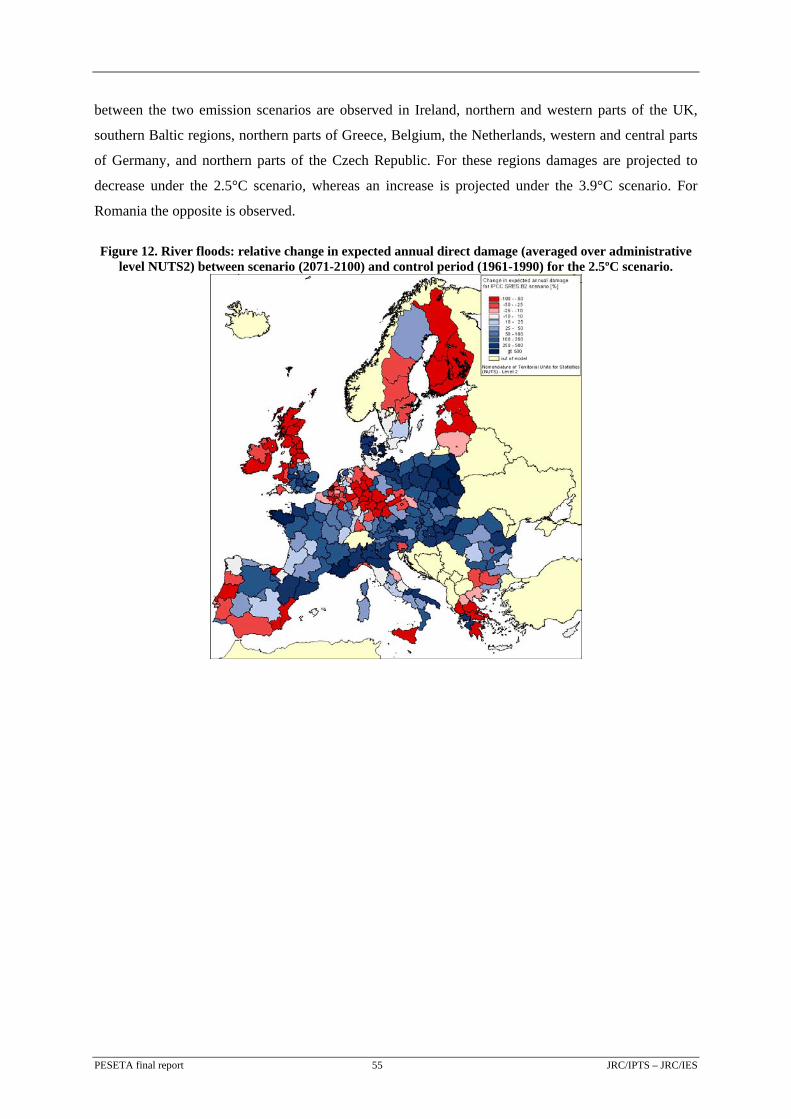
between the two emission scenarios are observed in Ireland, northern and western parts of the UK,
southern Baltic regions, northern parts of Greece, Belgium, the Netherlands, western and central parts
of Germany, and northern parts of the Czech Republic. For these regions damages are projected to
decrease under the 2.5°C scenario, whereas an increase is projected under the 3.9°C scenario. For
Romania the opposite is observed.
Figure 12. River floods: relative change in expected annual direct damage (averaged over administrative level NUTS2) between scenario (2071-2100) and control period (1961-1990) for the 2.5ºC scenario.
PESETA final report 55 JRC/IPTS – JRC/IES

Figure 13. River floods: relative change in expected annual direct damage (averaged over administrative level NUTS2) between scenario (2071-2100) and control period (1961-1990) for the 3.9ºC scenario
PESETA final report 56 JRC/IPTS – JRC/IES
5 COASTAL SYSTEMS ASSESSMENT
Coastal regions are areas where wealth and population are concentrated and are undergoing rapid
increases in population and urbanisation (McGranahan et al., 2007). Sea level rise is a direct threat for
productive infrastructures and for the residential and natural heritage zones.
This chapter summarises the methodology and the main results of the coastal systems impact and
adaptation assessment. Detailed information can be found in the accompanying PESETA technical
report Richards and Nicholls (2009).
5.1 Modelling approach in coastal systems
5.1.1 Coastal system model
Sea level rise (SLR) will have major direct impacts in Europe. Impacts of sea level rise in coastal
systems have been quantified with the DIVA model (Hinkel and Klein, 2006; McFadden, et al., 2007;
Nicholls and Klein, 2005; Nicholls et al., 2006; Nicholls et al., 2007; Vafeidis et al., 2004). DIVA
operates at the level of the individual linear coastal segments, which are independently considered.
The model database contains over 80 parameters for each variable-length segment that are utilized to
fully describe the physical characteristics of the coastline. The model calculates the impacts of sea-
level rise on each of these coastline segments, including direct coastal erosion, coastal flood impacts,
changes in wetlands, flood effects in river mouths, sea water intrusion and salinisation. The economic
costs due to land and wetland loss (related to erosion and flooding) and the number of people flooded
are computed in the economic module of DIVA.
DIVA has an adaptation module that controls a range of possible adaptation responses. This allows
giving more realistic estimates of impacts, costs and adaptation for a range of SLR scenarios (Nicholls
et al., 2007b). In this analysis, adaptation costs include (1) dike building and (2) beach nourishment (to
counter beach erosion), with the decisions on adaptation being based on cost-benefit analysis. The
results of the assessment show that in Europe adaptation is widespread, reflecting the large economic
values located in many coastal zones.
Table 13 shows the SLR for all scenarios considered. For each of the climate scenarios a low, medium
and high SLR case has been considered (Gordon et al,. 2000; Roeckener et al., 1996), in order to
account for the uncertainty in the future SLR. In addition, impacts are computed for the low and high
IPCC sea-level rise figures (Church et al., 2001). The IPCC Third Assessment Report (TAR) high and
low scenarios encompass the full range of uncertainty in sea-level rise projections (IPCC, 2001),
excluding uncertainties due to ice sheet instability and melting in Antarctica.
PESETA final report 57 JRC/IPTS – JRC/IES
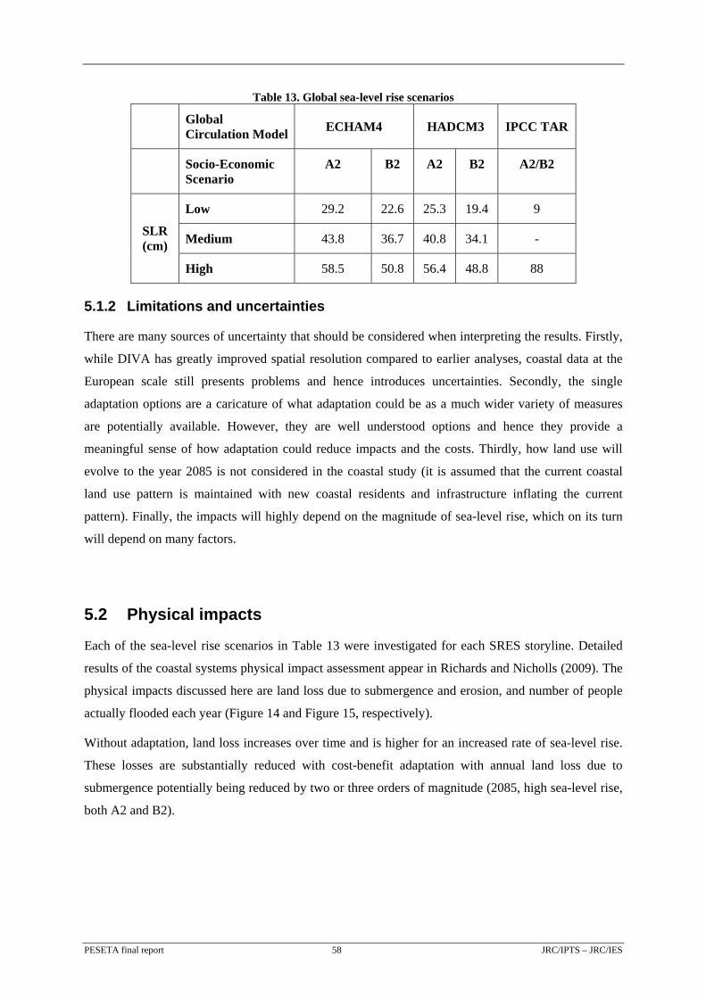
Table 13. Global sea-level rise scenarios
Global Circulation Model ECHAM4 HADCM3 IPCC TAR
Socio-Economic Scenario
A2 B2 A2 B2 A2/B2
Low 29.2 22.6 25.3 19.4 9
Medium 43.8 36.7 40.8 34.1 - SLR (cm)
High 58.5 50.8 56.4 48.8 88
5.1.2 Limitations and uncertainties
There are many sources of uncertainty that should be considered when interpreting the results. Firstly,
while DIVA has greatly improved spatial resolution compared to earlier analyses, coastal data at the
European scale still presents problems and hence introduces uncertainties. Secondly, the single
adaptation options are a caricature of what adaptation could be as a much wider variety of measures
are potentially available. However, they are well understood options and hence they provide a
meaningful sense of how adaptation could reduce impacts and the costs. Thirdly, how land use will
evolve to the year 2085 is not considered in the coastal study (it is assumed that the current coastal
land use pattern is maintained with new coastal residents and infrastructure inflating the current
pattern). Finally, the impacts will highly depend on the magnitude of sea-level rise, which on its turn
will depend on many factors.
5.2 Physical impacts
Each of the sea-level rise scenarios in Table 13 were investigated for each SRES storyline. Detailed
results of the coastal systems physical impact assessment appear in Richards and Nicholls (2009). The
physical impacts discussed here are land loss due to submergence and erosion, and number of people
actually flooded each year (Figure 14 and Figure 15, respectively).
Without adaptation, land loss increases over time and is higher for an increased rate of sea-level rise.
These losses are substantially reduced with cost-benefit adaptation with annual land loss due to
submergence potentially being reduced by two or three orders of magnitude (2085, high sea-level rise,
both A2 and B2).
PESETA final report 58 JRC/IPTS – JRC/IES
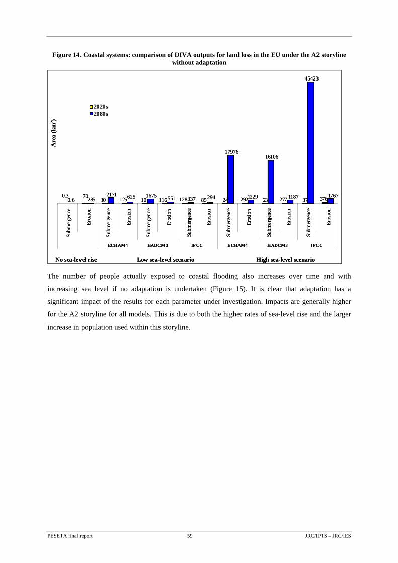
Figure 14. Coastal systems: comparison of DIVA outputs for land loss in the EU under the A2 storyline without adaptation
24 23 370.6 2852171 1675 551 337
1797616106
45423
376277292851281161012510700.3 176711871229294625
Subm
erge
nce
Eros
ion
Subm
erge
nce
Eros
ion
Subm
erge
nce
Eros
ion
Subm
erge
nce
Eros
ion
Subm
erge
nce
Eros
ion
Subm
erge
nce
Eros
ion
Subm
erge
nce
Eros
ion
ECHAM4 HADCM 3 IP CC ECHAM4 HADCM3 IPCC
No sea-level rise Low sea-level scenario High sea-level scenario
Are
a (k
m2 )
2020s2080s
The number of people actually exposed to coastal flooding also increases over time and with
increasing sea level if no adaptation is undertaken (Figure 15). It is clear that adaptation has a
significant impact of the results for each parameter under investigation. Impacts are generally higher
for the A2 storyline for all models. This is due to both the higher rates of sea-level rise and the larger
increase in population used within this storyline.
PESETA final report 59 JRC/IPTS – JRC/IES
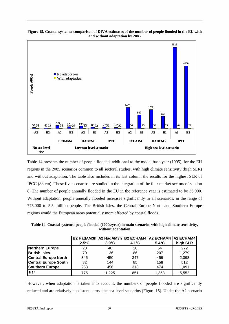
Figure 15. Coastal systems: comparison of DIVA estimates of the number of people flooded in the EU with and without adaptation by 2085
52 41219 101 135 83 76 62
1420
910
1292
833
5625
4330
31 22 33 23 33 23 32 22 36 25 36 25 40 28
A2 B2 A2 B2 A2 B2 A2 B2 A2 B2 A2 B2 A2 B2
ECHAM4 HADCM3 IPCC ECHAM4 HADCM3 IPCC
No sea-levelrise
Low sea-level scenario High sea-level scenario
Peop
le (0
00s) No adaptation
With adaptation
52 41219 101 135 83 76 62
1420
910
1292
833
5625
4330
31 22 33 23 33 23 32 22 36 25 36 25 40 28
A2 B2 A2 B2 A2 B2 A2 B2 A2 B2 A2 B2 A2 B2
ECHAM4 HADCM3 IPCC ECHAM4 HADCM3 IPCC
No sea-levelrise
Low sea-level scenario High sea-level scenario
Peop
le (0
00s) No adaptation
With adaptationNo adaptationWith adaptation
Table 14 presents the number of people flooded, additional to the model base year (1995), for the EU
regions in the 2085 scenarios common to all sectoral studies, with high climate sensitivity (high SLR)
and without adaptation. The table also includes in its last column the results for the highest SLR of
IPCC (88 cm). These five scenarios are studied in the integration of the four market sectors of section
8. The number of people annually flooded in the EU in the reference year is estimated to be 36,000.
Without adaptation, people annually flooded increases significantly in all scenarios, in the range of
775,000 to 5.5 million people. The British Isles, the Central Europe North and Southern Europe
regions would the European areas potentially more affected by coastal floods.
Table 14. Coastal systems: people flooded (1000s/year) in main scenarios with high climate sensitivity, without adaptation
B2 HadAM3h A2 HadAM3h B2 ECHAM4 A2 ECHAM4 A2 ECHAM42.5°C 3.9°C 4.1°C 5.4°C high SLR
Northern Europe 20 40 20 56 272British Isles 70 136 86 207 1,279Central Europe North 345 450 347 459 2,398Central Europe South 82 144 85 158 512Southern Europe 258 456 313 474 1,091EU 775 1,225 851 1,353 5,552
However, when adaptation is taken into account, the numbers of people flooded are significantly
reduced and are relatively consistent across the sea-level scenarios (Figure 15). Under the A2 scenario
PESETA final report 60 JRC/IPTS – JRC/IES
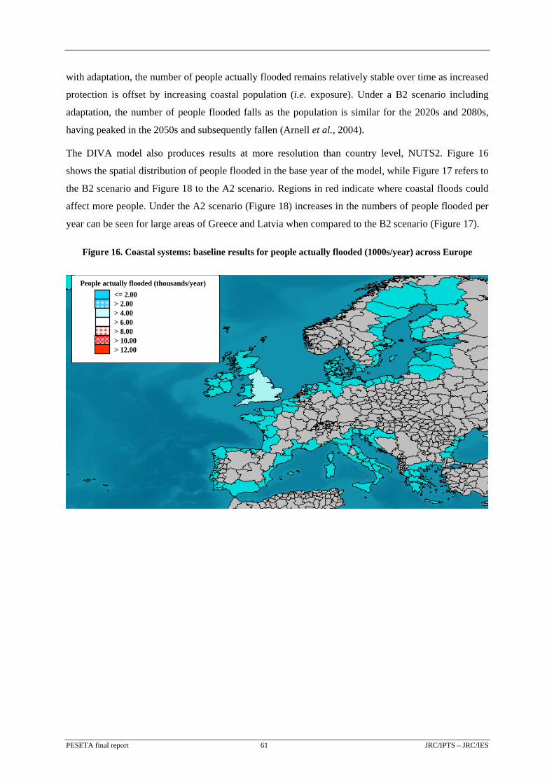
with adaptation, the number of people actually flooded remains relatively stable over time as increased
protection is offset by increasing coastal population (i.e. exposure). Under a B2 scenario including
adaptation, the number of people flooded falls as the population is similar for the 2020s and 2080s,
having peaked in the 2050s and subsequently fallen (Arnell et al., 2004).
The DIVA model also produces results at more resolution than country level, NUTS2. Figure 16
shows the spatial distribution of people flooded in the base year of the model, while Figure 17 refers to
the B2 scenario and Figure 18 to the A2 scenario. Regions in red indicate where coastal floods could
affect more people. Under the A2 scenario (Figure 18) increases in the numbers of people flooded per
year can be seen for large areas of Greece and Latvia when compared to the B2 scenario (Figure 17).
Figure 16. Coastal systems: baseline results for people actually flooded (1000s/year) across Europe
<= 2.00> 2.00> 4.00> 6.00> 8.00> 10.00> 12.00
People actually flooded (thousands/year)<= 2.00> 2.00> 4.00> 6.00> 8.00> 10.00> 12.00
People actually flooded (thousands/year)
PESETA final report 61 JRC/IPTS – JRC/IES
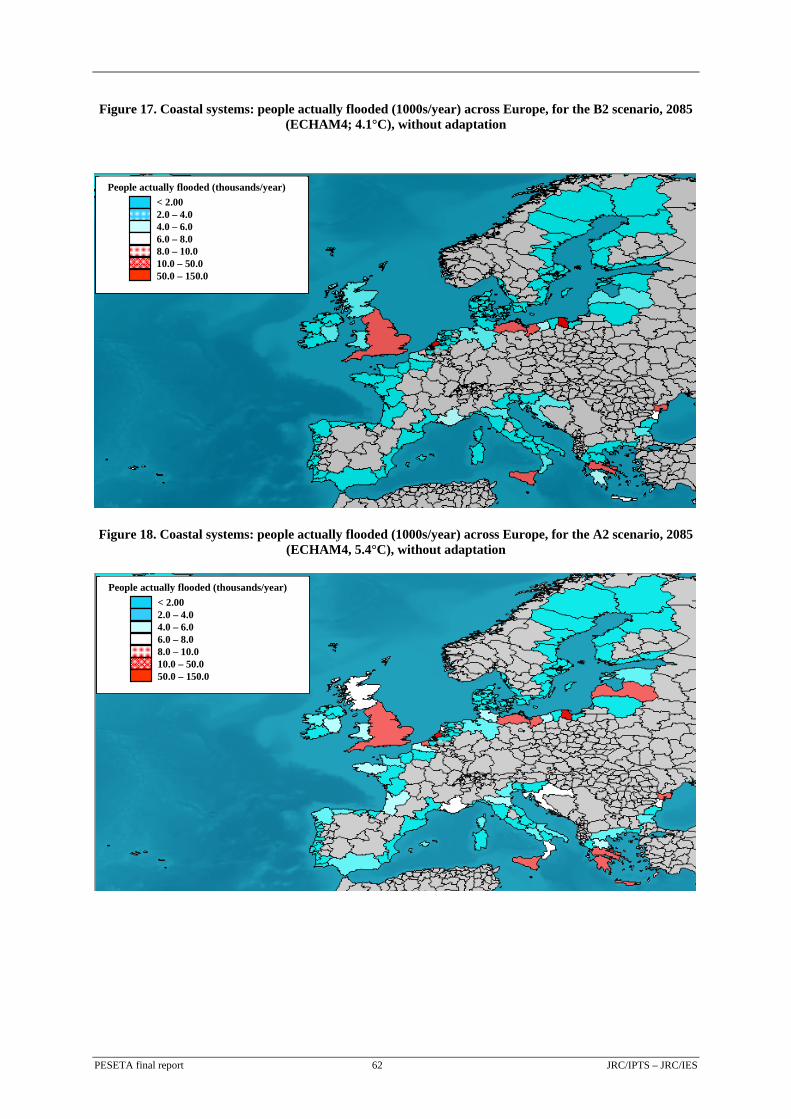
Figure 17. Coastal systems: people actually flooded (1000s/year) across Europe, for the B2 scenario, 2085 (ECHAM4; 4.1°C), without adaptation
< 2.002.0 – 4.04.0 – 6.06.0 – 8.08.0 – 10.010.0 – 50.050.0 – 150.0
People actually flooded (thousands/year)< 2.002.0 – 4.04.0 – 6.06.0 – 8.08.0 – 10.010.0 – 50.050.0 – 150.0
People actually flooded (thousands/year)< 2.002.0 – 4.04.0 – 6.06.0 – 8.08.0 – 10.010.0 – 50.050.0 – 150.0
People actually flooded (thousands/year)
Figure 18. Coastal systems: people actually flooded (1000s/year) across Europe, for the A2 scenario, 2085 (ECHAM4, 5.4°C), without adaptation
< 2.002.0 – 4.04.0 – 6.06.0 – 8.08.0 – 10.010.0 – 50.050.0 – 150.0
People actually flooded (thousands/year)< 2.002.0 – 4.04.0 – 6.06.0 – 8.08.0 – 10.010.0 – 50.050.0 – 150.0
People actually flooded (thousands/year)< 2.002.0 – 4.04.0 – 6.06.0 – 8.08.0 – 10.010.0 – 50.050.0 – 150.0
People actually flooded (thousands/year)
PESETA final report 62 JRC/IPTS – JRC/IES

5.3 Economic impacts
5.3.1 Direct economic effects
Table 15 and Table 16 show the range of estimates of economic damages for the 2020s and 2080s
from the DIVA model with and without optimal adaptation for the low SLR and high SLR range of the
IPCC TAR (9 cm and 88 cm, respectively). The tables show the three main climate cost components
in coastal systems: sea floods, salinity intrusion and migration costs. The residual damage means the
costs due to climate change, without considering adaptation costs. Adaptation costs include dike costs.
The net benefit of adaptation is the costs without adaptation minus the residual damage and the
adaptation costs.
The main results of the economic evaluation is that damage costs for the high rate of sea-level rise for
2085 are substantially higher than for a low rate of sea-level rise and both are substantially reduced if
adaptation is undertaken. Costs of people migrating due to land loss through submergence and erosion
are also substantially increased under a high rate of sea-level rise, assuming no adaptation, and
increase over time. When optimal adaptation options are included, this displacement of people
becomes a minor impact, showing the important benefit of adaptation to coastal populations under
rising sea levels.
Table 15. Coastal systems: EU Aggregated Results for IPCC A2 Economic Impacts, Highest Sea-level Rise (million €/year) (1995 values)
Adaptation Scenario Time slice
Total residual damage
costs
Sea Flood Costs
Salinity Intrusion
Costs
Migration (due to
land loss) costs
Adaptation Costs
Sea dike
costs
Net Benefit of
Adaptation
1995 1756.4 1159.6 588.3 0 0 0 -
No Adaptation 2020s 6636.8 6020.4 607.5 0.3 0 0 -
2080s 44605.6 18242.5 1053.3 25242.6 0 0 -
Optimal Adaptation 2020s 1727.2 1116.1 607.5 0.2 1013.4 628.3 3896.2
2080s 2241.6 1159.3 1053.3 20.1 2607.8 1356.9 39756.2
PESETA final report 63 JRC/IPTS – JRC/IES
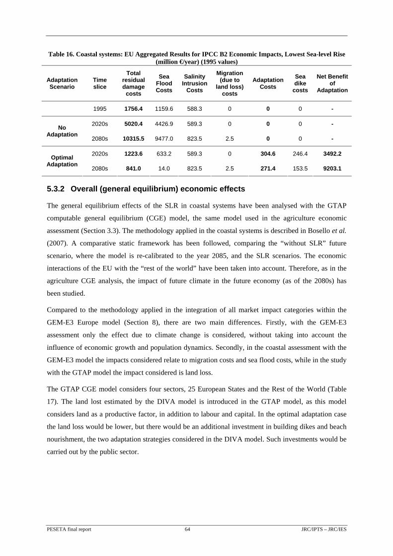
Table 16. Coastal systems: EU Aggregated Results for IPCC B2 Economic Impacts, Lowest Sea-level Rise (million €/year) (1995 values)
Adaptation Scenario
Time slice
Total residual damage
costs
Sea Flood Costs
Salinity Intrusion
Costs
Migration (due to
land loss) costs
Adaptation Costs
Sea dike
costs
Net Benefit of
Adaptation
1995 1756.4 1159.6 588.3 0 0 0 -
2020s 5020.4 4426.9 589.3 0 0 0 - No Adaptation
2080s 10315.5 9477.0 823.5 2.5 0 0 -
2020s 1223.6 633.2 589.3 0 304.6 246.4 3492.2 Optimal Adaptation
2080s 841.0 14.0 823.5 2.5 271.4 153.5 9203.1
5.3.2 Overall (general equilibrium) economic effects
The general equilibrium effects of the SLR in coastal systems have been analysed with the GTAP
computable general equilibrium (CGE) model, the same model used in the agriculture economic
assessment (Section 3.3). The methodology applied in the coastal systems is described in Bosello et al.
(2007). A comparative static framework has been followed, comparing the “without SLR” future
scenario, where the model is re-calibrated to the year 2085, and the SLR scenarios. The economic
interactions of the EU with the “rest of the world” have been taken into account. Therefore, as in the
agriculture CGE analysis, the impact of future climate in the future economy (as of the 2080s) has
been studied.
Compared to the methodology applied in the integration of all market impact categories within the
GEM-E3 Europe model (Section 8), there are two main differences. Firstly, with the GEM-E3
assessment only the effect due to climate change is considered, without taking into account the
influence of economic growth and population dynamics. Secondly, in the coastal assessment with the
GEM-E3 model the impacts considered relate to migration costs and sea flood costs, while in the study
with the GTAP model the impact considered is land loss.
The GTAP CGE model considers four sectors, 25 European States and the Rest of the World (Table
17). The land lost estimated by the DIVA model is introduced in the GTAP model, as this model
considers land as a productive factor, in addition to labour and capital. In the optimal adaptation case
the land loss would be lower, but there would be an additional investment in building dikes and beach
nourishment, the two adaptation strategies considered in the DIVA model. Such investments would be
carried out by the public sector.
PESETA final report 64 JRC/IPTS – JRC/IES
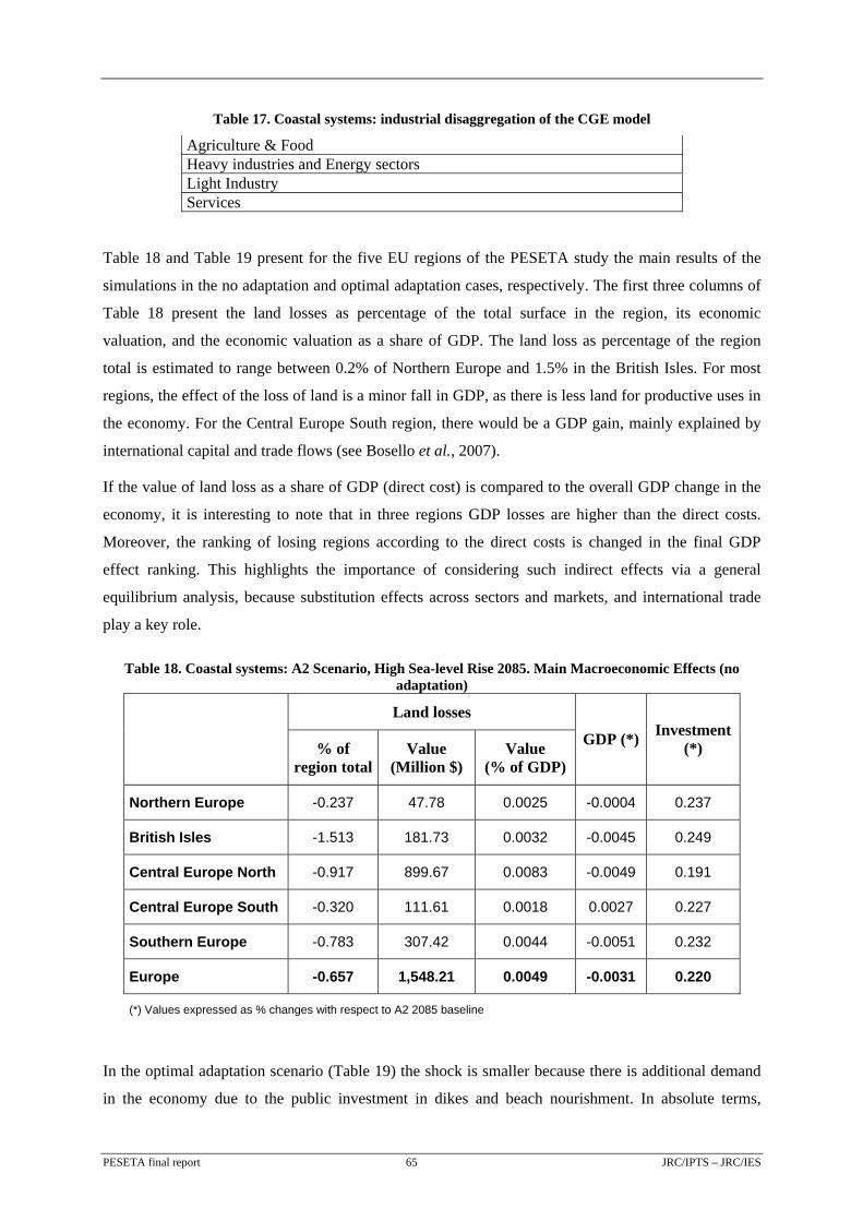
Table 17. Coastal systems: industrial disaggregation of the CGE model
Agriculture & Food Heavy industries and Energy sectors Light Industry Services
Table 18 and Table 19 present for the five EU regions of the PESETA study the main results of the
simulations in the no adaptation and optimal adaptation cases, respectively. The first three columns of
Table 18 present the land losses as percentage of the total surface in the region, its economic
valuation, and the economic valuation as a share of GDP. The land loss as percentage of the region
total is estimated to range between 0.2% of Northern Europe and 1.5% in the British Isles. For most
regions, the effect of the loss of land is a minor fall in GDP, as there is less land for productive uses in
the economy. For the Central Europe South region, there would be a GDP gain, mainly explained by
international capital and trade flows (see Bosello et al., 2007).
If the value of land loss as a share of GDP (direct cost) is compared to the overall GDP change in the
economy, it is interesting to note that in three regions GDP losses are higher than the direct costs.
Moreover, the ranking of losing regions according to the direct costs is changed in the final GDP
effect ranking. This highlights the importance of considering such indirect effects via a general
equilibrium analysis, because substitution effects across sectors and markets, and international trade
play a key role.
Table 18. Coastal systems: A2 Scenario, High Sea-level Rise 2085. Main Macroeconomic Effects (no adaptation)
Land losses
% of
region totalValue
(Million $) Value
(% of GDP)
GDP (*) Investment (*)
Northern Europe -0.237 47.78 0.0025 -0.0004 0.237
British Isles -1.513 181.73 0.0032 -0.0045 0.249
Central Europe North -0.917 899.67 0.0083 -0.0049 0.191
Central Europe South -0.320 111.61 0.0018 0.0027 0.227
Southern Europe -0.783 307.42 0.0044 -0.0051 0.232
Europe -0.657 1,548.21 0.0049 -0.0031 0.220
(*) Values expressed as % changes with respect to A2 2085 baseline
In the optimal adaptation scenario (Table 19) the shock is smaller because there is additional demand
in the economy due to the public investment in dikes and beach nourishment. In absolute terms,
PESETA final report 65 JRC/IPTS – JRC/IES
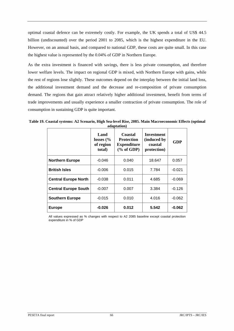
PESETA final report 66 JRC/IPTS – JRC/IES
optimal coastal defence can be extremely costly. For example, the UK spends a total of US$ 44.5
billion (undiscounted) over the period 2001 to 2085, which is the highest expenditure in the EU.
However, on an annual basis, and compared to national GDP, these costs are quite small. In this case
the highest value is represented by the 0.04% of GDP in Northern Europe.
As the extra investment is financed with savings, there is less private consumption, and therefore
lower welfare levels. The impact on regional GDP is mixed, with Northern Europe with gains, while
the rest of regions lose slightly. These outcomes depend on the interplay between the initial land loss,
the additional investment demand and the decrease and re-composition of private consumption
demand. The regions that gain attract relatively higher additional investment, benefit from terms of
trade improvements and usually experience a smaller contraction of private consumption. The role of
consumption in sustaining GDP is quite important.
Table 19. Coastal systems: A2 Scenario, High Sea-level Rise, 2085. Main Macroeconomic Effects (optimal adaptation)
Land losses (% of region
total)
Coastal Protection
Expenditure (% of GDP)
Investment (induced by
coastal protection)
GDP
Northern Europe -0.046 0.040 18.647 0.057
British Isles -0.006 0.015 7.784 -0.021
Central Europe North -0.038 0.011 4.685 -0.069
Central Europe South -0.007 0.007 3.384 -0.126
Southern Europe -0.015 0.010 4.016 -0.062
Europe -0.026 0.012 5.542 -0.062
All values expressed as % changes with respect to A2 2085 baseline except coastal protection expenditure in % of GDP
6 TOURISM ASSESSMENT
Tourism is a major economic sector in Europe, with the current annual flow of tourists from Northern
to Southern Europe accounting for one in every six tourist arrivals in the world (Mather et al., 2005).
Climate change has the potential to radically alter tourism patterns in Europe by inducing changes in
destinations and seasonal demand structure (Scott et al., 2008).
This chapter summarises the methodology and the main results of the study on the impact of climate
change in tourism in Europe. Detailed information can be found in the accompanying PESETA
technical report Amelung and Moreno (2009).
6.1 Tourism impact methodology
6.1.1 The modelling approach
The final aim of the endeavour was to model tourist activity, to estimate the role of climate, and to
explore the effects of climate change. The changes in visitation patterns were explored in two steps.
First a visitation model was estimated, based on historical data. Subsequently, the baseline and future
scenarios were simulated. The historical visitation model was developed using regression techniques.
The tourism study aims at modelling the major outdoor international tourism flows within Europe. The
study improves on earlier work because it integrates the climate component of tourist activity with the
economic analysis of tourist demand flows. Furthermore, it is the first study to consider seasonality
effects in a tourist regional demand model, a time dimension relevant to the modelling of aggregated
tourist flows.
Regarding the economic analysis of tourism demand, a tourism bed night equation with regional and
seasonal resolution has been statistically estimated with price levels, income, fixed seasonal effects
and a climate index as explanatory variables. Concerning the climate side, the influence of the climate
has been explicitly considered by having the tourism climatic index (TCI) in the demand equation. The
index is developed primarily for general outdoor activities by Mieczkoswki (1985), and therefore this
assessment excludes winter sports. TCI is based on the notion of 'human comfort' and consists of a
weighted index of maximum and mean daily temperature, humidity, precipitation, sunshine and wind.
The index was calculated for all NUTS2 regions for Europe and thus provides at high-resolution input
values for the estimations.
The impact of climate change on bed nights has been simulated with the estimated demand equation
changing the TCI index according to the climate scenarios, while the rest of the exogenous variables
of the model remain constant. The bed nights changes are interpreted as the physical impacts of
PESETA final report 67 JRC/IPTS – JRC/IES
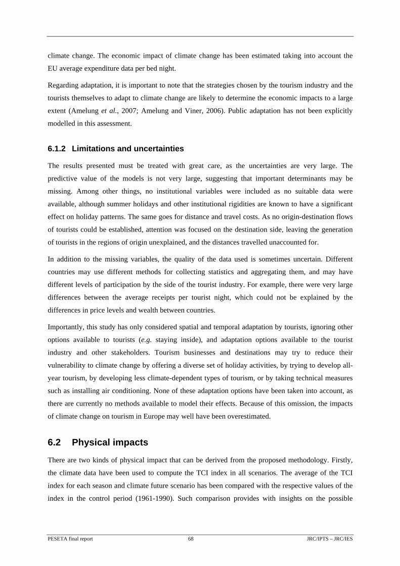
climate change. The economic impact of climate change has been estimated taking into account the
EU average expenditure data per bed night.
Regarding adaptation, it is important to note that the strategies chosen by the tourism industry and the
tourists themselves to adapt to climate change are likely to determine the economic impacts to a large
extent (Amelung et al., 2007; Amelung and Viner, 2006). Public adaptation has not been explicitly
modelled in this assessment.
6.1.2 Limitations and uncertainties
The results presented must be treated with great care, as the uncertainties are very large. The
predictive value of the models is not very large, suggesting that important determinants may be
missing. Among other things, no institutional variables were included as no suitable data were
available, although summer holidays and other institutional rigidities are known to have a significant
effect on holiday patterns. The same goes for distance and travel costs. As no origin-destination flows
of tourists could be established, attention was focused on the destination side, leaving the generation
of tourists in the regions of origin unexplained, and the distances travelled unaccounted for.
In addition to the missing variables, the quality of the data used is sometimes uncertain. Different
countries may use different methods for collecting statistics and aggregating them, and may have
different levels of participation by the side of the tourist industry. For example, there were very large
differences between the average receipts per tourist night, which could not be explained by the
differences in price levels and wealth between countries.
Importantly, this study has only considered spatial and temporal adaptation by tourists, ignoring other
options available to tourists (e.g. staying inside), and adaptation options available to the tourist
industry and other stakeholders. Tourism businesses and destinations may try to reduce their
vulnerability to climate change by offering a diverse set of holiday activities, by trying to develop all-
year tourism, by developing less climate-dependent types of tourism, or by taking technical measures
such as installing air conditioning. None of these adaptation options have been taken into account, as
there are currently no methods available to model their effects. Because of this omission, the impacts
of climate change on tourism in Europe may well have been overestimated.
6.2 Physical impacts
There are two kinds of physical impact that can be derived from the proposed methodology. Firstly,
the climate data have been used to compute the TCI index in all scenarios. The average of the TCI
index for each season and climate future scenario has been compared with the respective values of the
index in the control period (1961-1990). Such comparison provides with insights on the possible
PESETA final report 68 JRC/IPTS – JRC/IES
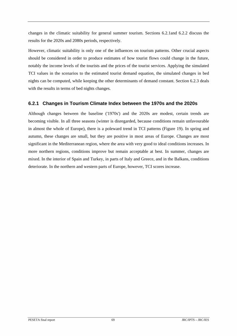
changes in the climatic suitability for general summer tourism. Sections 6.2.1and 6.2.2 discuss the
results for the 2020s and 2080s periods, respectively.
However, climatic suitability is only one of the influences on tourism patterns. Other crucial aspects
should be considered in order to produce estimates of how tourist flows could change in the future,
notably the income levels of the tourists and the prices of the tourist services. Applying the simulated
TCI values in the scenarios to the estimated tourist demand equation, the simulated changes in bed
nights can be computed, while keeping the other determinants of demand constant. Section 6.2.3 deals
with the results in terms of bed nights changes.
6.2.1 Changes in Tourism Climate Index between the 1970s and the 2020s
Although changes between the baseline ('1970s') and the 2020s are modest, certain trends are
becoming visible. In all three seasons (winter is disregarded, because conditions remain unfavourable
in almost the whole of Europe), there is a poleward trend in TCI patterns (Figure 19). In spring and
autumn, these changes are small, but they are positive in most areas of Europe. Changes are most
significant in the Mediterranean region, where the area with very good to ideal conditions increases. In
more northern regions, conditions improve but remain acceptable at best. In summer, changes are
mixed. In the interior of Spain and Turkey, in parts of Italy and Greece, and in the Balkans, conditions
deteriorate. In the northern and western parts of Europe, however, TCI scores increase.
PESETA final report 69 JRC/IPTS – JRC/IES
Figure 19. Tourism: TCI scores in spring (top), summer (middle) and autumn (bottom) in the 1970s (left) and the 2020s (right) according to the Rossby Centre RCA3 model
Ideal
Excellent
Very good
Good
Acceptable
Marginal
Unfavourable
Ideal
Excellent
Very good
Good
Acceptable
Marginal
Unfavourable
Ideal
Excellent
Very good
Good
Acceptable
Marginal
Unfavourable
PESETA final report 70 JRC/IPTS – JRC/IES
6.2.2 Changes in Tourism Climate Index between the 1970s and the 2080s
By the end of the 21st century, the distribution of climatic resources in Europe is projected to change
significantly. All four model-scenario combinations agree on this, but the magnitude of the change and
the evaluation of the initial conditions differ.
For the spring season (Figure 20 and Figure 21), all climate model results show a clear extension
towards the North of the zone with good conditions, with also better conditions in the South.
Compared to the RCAO model (Figure 21), the Hirham model projects relatively modest changes, in
accordance with the projected warming trends in the EU. In the 3.9°C scenario, spring conditions
would have become very good to excellent in most of the Mediterranean by the end of the century.
Good conditions are projected to be more frequent in France and the Balkans. The same tendency is
visible in the 2.5°C scenario, albeit at a slower pace.
Figure 20. Tourism: TCI scores in spring in the 1970s (left) and the 2080s (right), according to the HIRHAM model, 3.9°C scenario (top) and 2.5°C scenario (bottom)
.
Ideal
Excellent
Very good
Good
Acceptable
Marginal
Unfavourable
PESETA final report 71 JRC/IPTS – JRC/IES
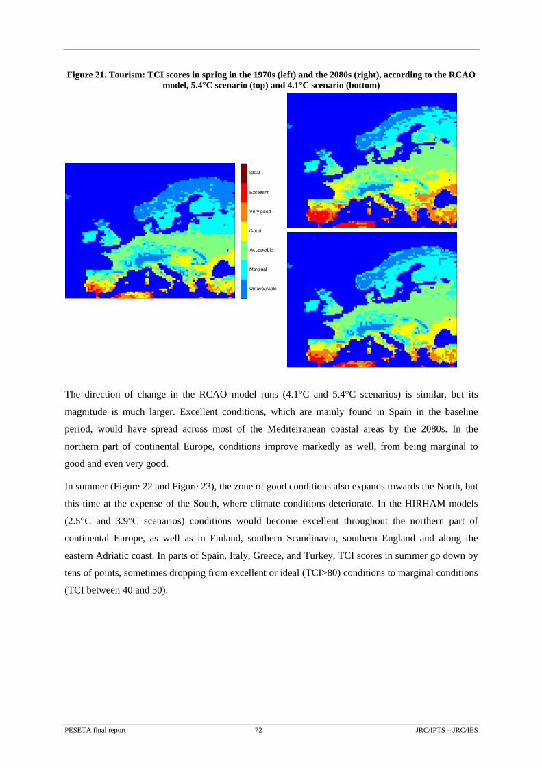
Figure 21. Tourism: TCI scores in spring in the 1970s (left) and the 2080s (right), according to the RCAO model, 5.4°C scenario (top) and 4.1°C scenario (bottom)
Ideal
Excellent
Very good
Good
Acceptable
Marginal
Unfavourable
The direction of change in the RCAO model runs (4.1°C and 5.4°C scenarios) is similar, but its
magnitude is much larger. Excellent conditions, which are mainly found in Spain in the baseline
period, would have spread across most of the Mediterranean coastal areas by the 2080s. In the
northern part of continental Europe, conditions improve markedly as well, from being marginal to
good and even very good.
In summer (Figure 22 and Figure 23), the zone of good conditions also expands towards the North, but
this time at the expense of the South, where climate conditions deteriorate. In the HIRHAM models
(2.5°C and 3.9°C scenarios) conditions would become excellent throughout the northern part of
continental Europe, as well as in Finland, southern Scandinavia, southern England and along the
eastern Adriatic coast. In parts of Spain, Italy, Greece, and Turkey, TCI scores in summer go down by
tens of points, sometimes dropping from excellent or ideal (TCI>80) conditions to marginal conditions
(TCI between 40 and 50).
PESETA final report 72 JRC/IPTS – JRC/IES
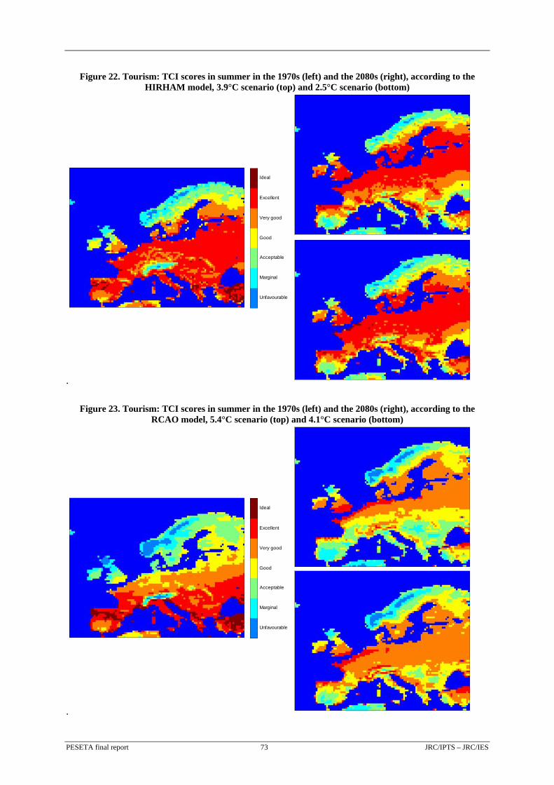
Figure 22. Tourism: TCI scores in summer in the 1970s (left) and the 2080s (right), according to the HIRHAM model, 3.9°C scenario (top) and 2.5°C scenario (bottom)
.
Ideal
Excellent
Very good
Good
Acceptable
Marginal
Unfavourable
Figure 23. Tourism: TCI scores in summer in the 1970s (left) and the 2080s (right), according to the RCAO model, 5.4°C scenario (top) and 4.1°C scenario (bottom)
.
Ideal
Excellent
Very good
Good
Acceptable
Marginal
Unfavourable
PESETA final report 73 JRC/IPTS – JRC/IES
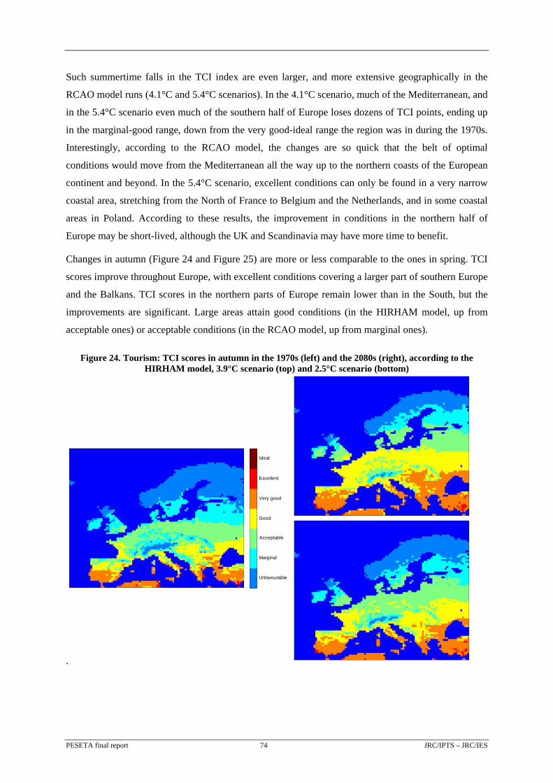
Such summertime falls in the TCI index are even larger, and more extensive geographically in the
RCAO model runs (4.1°C and 5.4°C scenarios). In the 4.1°C scenario, much of the Mediterranean, and
in the 5.4°C scenario even much of the southern half of Europe loses dozens of TCI points, ending up
in the marginal-good range, down from the very good-ideal range the region was in during the 1970s.
Interestingly, according to the RCAO model, the changes are so quick that the belt of optimal
conditions would move from the Mediterranean all the way up to the northern coasts of the European
continent and beyond. In the 5.4°C scenario, excellent conditions can only be found in a very narrow
coastal area, stretching from the North of France to Belgium and the Netherlands, and in some coastal
areas in Poland. According to these results, the improvement in conditions in the northern half of
Europe may be short-lived, although the UK and Scandinavia may have more time to benefit.
Changes in autumn (Figure 24 and Figure 25) are more or less comparable to the ones in spring. TCI
scores improve throughout Europe, with excellent conditions covering a larger part of southern Europe
and the Balkans. TCI scores in the northern parts of Europe remain lower than in the South, but the
improvements are significant. Large areas attain good conditions (in the HIRHAM model, up from
acceptable ones) or acceptable conditions (in the RCAO model, up from marginal ones).
Figure 24. Tourism: TCI scores in autumn in the 1970s (left) and the 2080s (right), according to the HIRHAM model, 3.9°C scenario (top) and 2.5°C scenario (bottom)
.
Ideal
Excellent
Very good
Good
Acceptable
Marginal
Unfavourable
PESETA final report 74 JRC/IPTS – JRC/IES
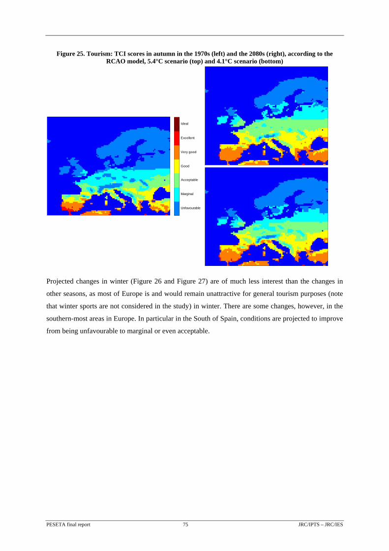
Figure 25. Tourism: TCI scores in autumn in the 1970s (left) and the 2080s (right), according to the RCAO model, 5.4°C scenario (top) and 4.1°C scenario (bottom)
Ideal
Excellent
Very good
Good
Acceptable
Marginal
Unfavourable
Projected changes in winter (Figure 26 and Figure 27) are of much less interest than the changes in
other seasons, as most of Europe is and would remain unattractive for general tourism purposes (note
that winter sports are not considered in the study) in winter. There are some changes, however, in the
southern-most areas in Europe. In particular in the South of Spain, conditions are projected to improve
from being unfavourable to marginal or even acceptable.
PESETA final report 75 JRC/IPTS – JRC/IES
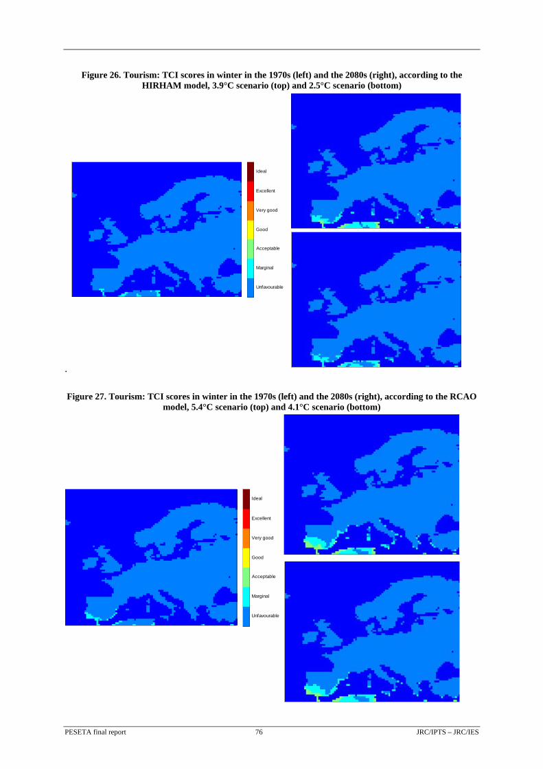
Figure 26. Tourism: TCI scores in winter in the 1970s (left) and the 2080s (right), according to the HIRHAM model, 3.9°C scenario (top) and 2.5°C scenario (bottom)
.
Ideal
Excellent
Very good
Good
Acceptable
Marginal
Unfavourable
Figure 27. Tourism: TCI scores in winter in the 1970s (left) and the 2080s (right), according to the RCAO model, 5.4°C scenario (top) and 4.1°C scenario (bottom)
Ideal
Excellent
Very good
Good
Acceptable
Marginal
Unfavourable
PESETA final report 76 JRC/IPTS – JRC/IES
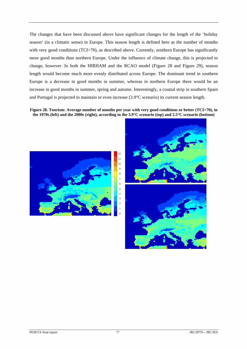
The changes that have been discussed above have significant changes for the length of the ‘holiday
season‘ (in a climatic sense) in Europe. This season length is defined here as the number of months
with very good conditions (TCI>70), as described above. Currently, southern Europe has significantly
more good months than northern Europe. Under the influence of climate change, this is projected to
change, however. In both the HIRHAM and the RCAO model (Figure 28 and Figure 29), season
length would become much more evenly distributed across Europe. The dominant trend in southern
Europe is a decrease in good months in summer, whereas in northern Europe there would be an
increase in good months in summer, spring and autumn. Interestingly, a coastal strip in southern Spain
and Portugal is projected to maintain or even increase (3.9°C scenario) its current season length.
Figure 28. Tourism: Average number of months per year with very good conditions or better (TCI>70), in the 1970s (left) and the 2080s (right), according to the 3.9°C scenario (top) and 2.5°C scenario (bottom)
12
11
10
9
8
6
7
5
4
3
2
1
0
PESETA final report 77 JRC/IPTS – JRC/IES
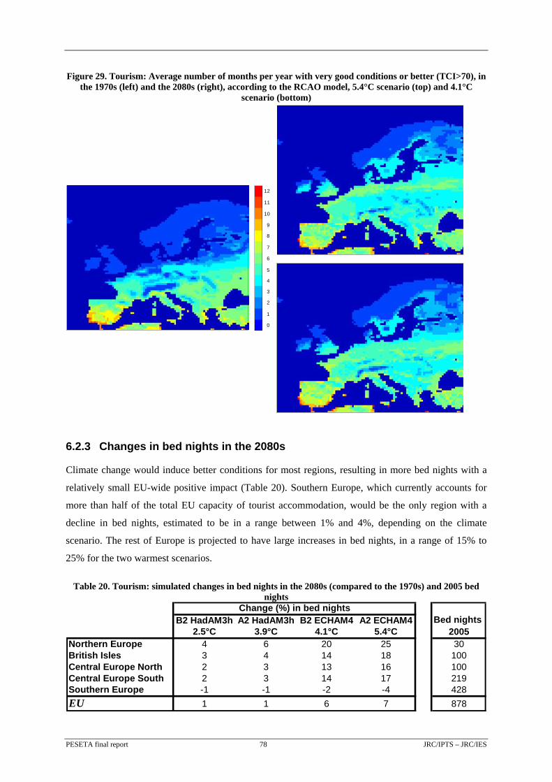
Figure 29. Tourism: Average number of months per year with very good conditions or better (TCI>70), in the 1970s (left) and the 2080s (right), according to the RCAO model, 5.4°C scenario (top) and 4.1°C
scenario (bottom)
12
11
10
9
8
6
7
5
4
3
2
1
0
6.2.3 Changes in bed nights in the 2080s
Climate change would induce better conditions for most regions, resulting in more bed nights with a
relatively small EU-wide positive impact (Table 20). Southern Europe, which currently accounts for
more than half of the total EU capacity of tourist accommodation, would be the only region with a
decline in bed nights, estimated to be in a range between 1% and 4%, depending on the climate
scenario. The rest of Europe is projected to have large increases in bed nights, in a range of 15% to
25% for the two warmest scenarios.
Table 20. Tourism: simulated changes in bed nights in the 2080s (compared to the 1970s) and 2005 bed nights
B2 HadAM3h A2 HadAM3h B2 ECHAM4 A2 ECHAM42.5°C 3.9°C 4.1°C 5.4°C
Northern Europe 4 6 20 25 30British Isles 3 4 14 18 100Central Europe North 2 3 13 16 100Central Europe South 2 3 14 17 219Southern Europe -1 -1 -2 -4 428EU 1 1 6 7 878
Bed nights 2005
Change (%) in bed nights
PESETA final report 78 JRC/IPTS – JRC/IES
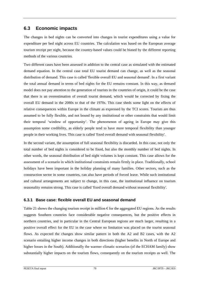
6.3 Economic impacts
The changes in bed nights can be converted into changes in tourist expenditures using a value for
expenditure per bed night across EU countries. The calculation was based on the European average
tourism receipt per night, because the country-based values could be biased by the different reporting
methods of the various countries.
Two different cases have been assessed in addition to the central case as simulated with the estimated
demand equation. In the central case total EU tourist demand can change, as well as the seasonal
distribution of demand. This case is called 'flexible overall EU and seasonal demand'. In a first variant
the total annual demand in terms of bed nights for the EU remains constant. In this way, as demand
model does not pay attention to the generation of tourists in the countries of origin, it could be the case
that there is an overestimation of overall tourist demand, which would be corrected by fixing the
overall EU demand in the 2080s to that of the 1970s. This case sheds some light on the effects of
relative consequences within Europe in the climate as expressed by the TCI scores. Tourists are thus
assumed to be fully flexible, and not bound by any institutional or other constraints that would limit
their temporal ‘window of opportunity’. The phenomenon of ageing in Europe may give this
assumption some credibility, as elderly people tend to have more temporal flexibility than younger
people in their working lives. This case is called 'fixed overall demand with seasonal flexibility'.
In the second variant, the assumption of full seasonal flexibility is discarded. In this case, not only the
total number of bed nights is considered to be fixed, but also the monthly number of bed nights. In
other words, the seasonal distribution of bed night volumes is kept constant. This case allows for the
assessment of a scenario in which institutional constraints remain firmly in place. Traditionally, school
holidays have been important in the holiday planning of many families. Other sectors, such as the
construction sector in some countries, can also have periods of forced leave. While such institutional
and cultural arrangements are subject to change, in this case, the institutional influence on tourism
seasonality remains strong. This case is called 'fixed overall demand without seasonal flexibility'.
6.3.1 Base case: flexible overall EU and seasonal demand
Table 21 shows the changing tourism receipt in million € for the aggregated EU regions. As the results
suggests Southern countries face considerable negative consequences, but the positive effects in
northern countries, and in particular in the Central European regions are much larger, resulting in a
positive overall effect for the EU in the case where no limitation was placed on the tourist seasonal
flows. As expected the changes show similar pattern in both the A2 and B2 cases, with the A2
scenario entailing higher income changes in both directions (higher benefits in North of Europe and
higher losses in the South). Additionally the warmer climatic scenarios (of the ECHAM family) show
substantially higher impacts on the tourism flows, consequently on the tourism receipts as well. The
PESETA final report 79 JRC/IPTS – JRC/IES
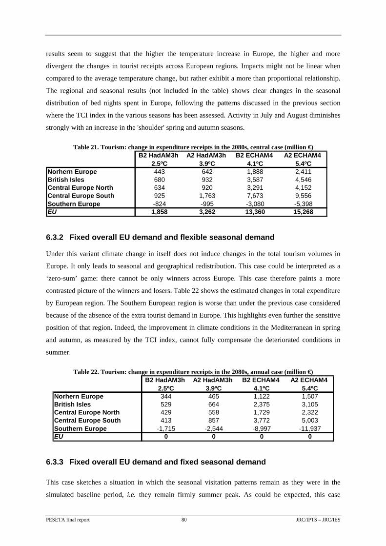
results seem to suggest that the higher the temperature increase in Europe, the higher and more
divergent the changes in tourist receipts across European regions. Impacts might not be linear when
compared to the average temperature change, but rather exhibit a more than proportional relationship.
The regional and seasonal results (not included in the table) shows clear changes in the seasonal
distribution of bed nights spent in Europe, following the patterns discussed in the previous section
where the TCI index in the various seasons has been assessed. Activity in July and August diminishes
strongly with an increase in the 'shoulder' spring and autumn seasons.
Table 21. Tourism: change in expenditure receipts in the 2080s, central case (million €) B2 HadAM3h
2.5ºCA2 HadAM3h
3.9ºCB2 ECHAM4
4.1ºCA2 ECHAM4
5.4ºCNorhern Europe 443 642 1,888 2,411British Isles 680 932 3,587 4,546Central Europe North 634 920 3,291 4,152Central Europe South 925 1,763 7,673 9,556Southern Europe -824 -995 -3,080 -5,398EU 1,858 3,262 13,360 15,268
6.3.2 Fixed overall EU demand and flexible seasonal demand
Under this variant climate change in itself does not induce changes in the total tourism volumes in
Europe. It only leads to seasonal and geographical redistribution. This case could be interpreted as a
‘zero-sum’ game: there cannot be only winners across Europe. This case therefore paints a more
contrasted picture of the winners and losers. Table 22 shows the estimated changes in total expenditure
by European region. The Southern European region is worse than under the previous case considered
because of the absence of the extra tourist demand in Europe. This highlights even further the sensitive
position of that region. Indeed, the improvement in climate conditions in the Mediterranean in spring
and autumn, as measured by the TCI index, cannot fully compensate the deteriorated conditions in
summer.
Table 22. Tourism: change in expenditure receipts in the 2080s, annual case (million €) B2 HadAM3h
2.5ºCA2 HadAM3h
3.9ºCB2 ECHAM4
4.1ºCA2 ECHAM4
5.4ºCNorhern Europe 344 465 1,122 1,507British Isles 529 664 2,375 3,105Central Europe North 429 558 1,729 2,322Central Europe South 413 857 3,772 5,003Southern Europe -1,715 -2,544 -8,997 -11,937EU 0 0 0 0
6.3.3 Fixed overall EU demand and fixed seasonal demand
This case sketches a situation in which the seasonal visitation patterns remain as they were in the
simulated baseline period, i.e. they remain firmly summer peak. As could be expected, this case
PESETA final report 80 JRC/IPTS – JRC/IES
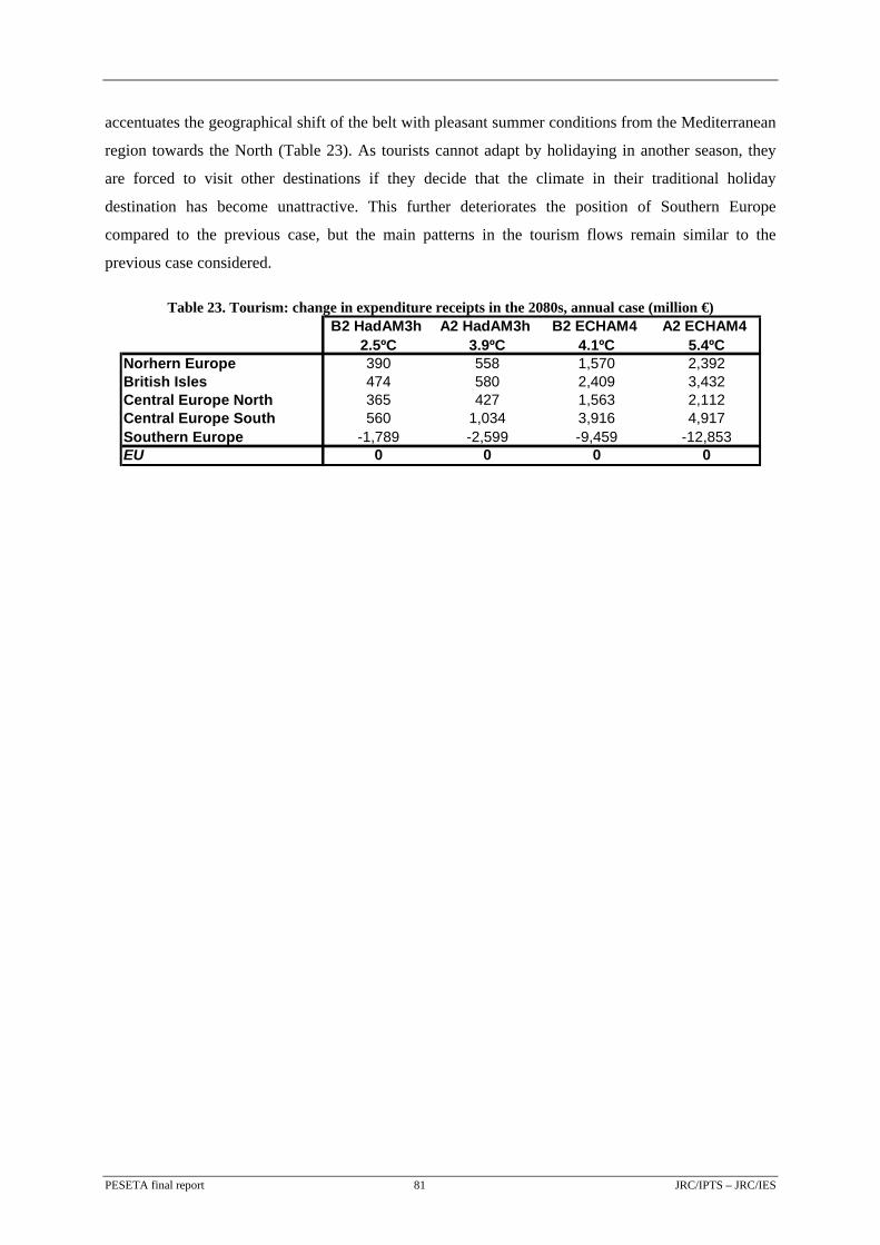
accentuates the geographical shift of the belt with pleasant summer conditions from the Mediterranean
region towards the North (Table 23). As tourists cannot adapt by holidaying in another season, they
are forced to visit other destinations if they decide that the climate in their traditional holiday
destination has become unattractive. This further deteriorates the position of Southern Europe
compared to the previous case, but the main patterns in the tourism flows remain similar to the
previous case considered.
Table 23. Tourism: change in expenditure receipts in the 2080s, annual case (million €) B2 HadAM3h
2.5ºCA2 HadAM3h
3.9ºCB2 ECHAM4
4.1ºCA2 ECHAM4
5.4ºCNorhern Europe 390 558 1,570 2,392British Isles 474 580 2,409 3,432Central Europe North 365 427 1,563 2,112Central Europe South 560 1,034 3,916 4,917Southern Europe -1,789 -2,599 -9,459 -12,853EU 0 0 0 0
PESETA final report 81 JRC/IPTS – JRC/IES


7 HUMAN HEALTH ASSESSMENT
Human health will be affected by climate change, in direct and indirect ways (Costello et al., 2009).
Effects include increases in summer heat related mortality, decreases in winter cold related mortality,
changes in the disease burden e.g. from vector-, water- or food-borne disease, and increases in the risk
of accidents and wider well being from extreme events (storms and floods).
This chapter summarises the methodology and the main results of the study on the impact of climate
change in human health in Europe. Here the results concerning direct temperature mortality changes
are discussed. Detailed information on the methodology and other results (e.g. temperature-related
cases of salmonella) can be found in the accompanying PESETA technical report Watkiss et al.
(2009).
7.1 Human health model
7.1.1 Modelling approach
The human health impact assessment of the PESETA project estimates projected mortality from
temperature changes for the 2020s and the 2080s across Europe.
The projections were based on relationships between mortality and current temperature
(epidemiological studies) available at the time. These mainly draw on the EU-funded cCASHh project
Menne and Ebi (2006) and work by Kovats et al (2006). Since the study was undertaken, a set of
country specific summer mortality functions for Europe have been published, as part of the PHEWE
study (Baccini et al., 2008).
The study used daily projected temperature information at a 50 km by 50 km grid resolution across
Europe, combined with country specific socio-economic scenario data for population, age structure
and background health incidence data for both current and future periods.
Impacts were estimated using temperature-response functions, which provide relationships of daily
mortality against daily temperature. These are usually represented as separate functions for heat and
cold effects, reflecting the fact that mortality increases at low or high temperatures above certain
threshold levels, i.e. around a broad central range over which there is little response. The functional
form of the relationships can vary, but in this study the functions were applied linearly above (heat) or
below (cold) specific thresholds, noting that different thresholds were used for each grid cell or
country.
PESETA final report 83 JRC/IPTS – JRC/IES
It is stressed that applying functions from the current climate to future modelled projections is
extremely uncertain. There are issues of which functions to use, what level of spatial scale and
location they are appropriate for (their transferability), how well they capture changes in both the
mean and variance of future temperatures and how applicable they are to future societies. Another key
issue is the degree of autonomous acclimatisation over time (physiological and behavioural) –
discussed below - that is likely to occur among European populations.
While the overall PESETA study has considered some limited analysis of the uncertainty of climate
projections through the use of two alternative models and two socio-economic scenarios, the added
uncertainty from the impact functions (and valuation, see later) will also have a very large effect on
the results and the subsequent policy messages. The health study has therefore applied alternative
functions and assumptions to investigate the effects on the results – at an aggregated level – and in
relation to the distribution of effects by location.
The study has used two approaches for assessing heat- and cold-related temperature effects
• Country specific functions, which are based on functions identified under the cCASHh project
(Menne and Ebi, 2006) for specific European countries (where available). These included
functions for Norway, Finland, Bulgaria, UK, Netherlands, Spain and Greece, each of which has a
specific threshold level and a specific slope (or gradient). These functions were applied to each
country and to climatically and socially similar countries nearby. These functions more accurately
represent current physiological and social conditions, the existing adaptation to the current climate
and sensitivity to existing climate variation. However, the functions derived have a partial
coverage and come from different studies. Note that since this study, a consistent set of heat
related functions have been published by Baccini et al. (2008).
• Climate-dependent functions, based on an extension of an approach adopted by Kovats et al.
(2006). This involved a more complex approach, first estimating heat and cold thresholds for each
50 by 50 km location in Europe using a statistical analysis of daily temperatures. This established
thresholds in each grid cell for low- and high-temperatures. The study then applied a single
consistent function (a fixed single slope) for each of heat and cold related mortality in each cell,
assuming a linear form beyond the threshold point. The advantage of this approach is it has a
higher resolution and allows greater coverage across all specific locations and a potentially better
representation of local thresholds. It also allows a more direct comparison of the relative level of
warming seen across Europe in the model output, as it adopts a more directly comparable
approach. The downside is the application of a single function (identical slope) in all grid cells and
thus the lack of consideration of country specific vulnerability.
PESETA final report 84 JRC/IPTS – JRC/IES

The study also considered acclimatisation, which is likely to reduce potential increases in heat-related
mortality. Whilst some studies incorporate acclimatisation into future projections of temperature-
related mortality there is no consensus on the analytical approach. The study has adopted the fixed rate
approach used by Dessai (2003) and assumed acclimatisation to 1ºC warming occurs every three
decades. This is only very approximate, but it does provide some representation of physiological
adaptation. Note that in practice, acclimatisation rates will be scenario- and location- specific
according to the rate of warming experienced and the susceptibility or resilience to future changes.
Note that this acclimatisation does not include additional planned adaptation. The study assumes that
populations acclimatise to a warmer climate in the future, modelled through a shift in threshold
temperatures. It is noted that there are many assumptions in this approach and it can only be
considered indicative. It is uncertain whether there will also be a decline in the sensitivity of mortality
to cold. There is no specific literature on this subject but some anecdotal evidence. As a sensitivity, the
study has investigated the potential effects for a decline in the sensitivity of mortality to cold, using
similar rates as assumed for heat. It is highlighted that the confidence in this estimate is low.
In addition to acclimatisation, planned, proactive adaptation may have a strong role in reducing
potential health risks, particularly in relation to extremes. There are emerging studies on adaptation
strategies that can be implemented by health sectors (Menne and Ebi, 2006), most of which build on
well-established public health approaches. They include
• Strengthening of effective surveillance and prevention programmes
• Sharing lessons learned across countries and sectors
• Introducing new prevention measures or increasing existing measures
• Development of new policies to address new threats
The main problem with assessing the potential for adaptation to reduce impacts is a lack of
information on the effectiveness of adaptation measures in reducing potential impacts. While some
estimates of potential costs are starting to emerge, such as heatwave health plans in France and Paris
(Mairie de Paris, 2007) it remains difficult to estimate and attribute potential benefits. For these
reasons, an explicit assessment of the costs and benefits of adaptation for heat related effects has not
been undertaken.
There is also a strong link between the potential temperature effects on human health and demand for
energy, in relation to the role of air conditioning as an adaptation. As countries experience warmer
climates, there will be a need to control these new environments or adjust human behaviour to deal
with these changes. Health (and well-being) will be a strong driver in this respect. One response is
PESETA final report 85 JRC/IPTS – JRC/IES
through air conditioning, though this will have implications for increasing energy use (see the energy
study). Planned adaptation therefore also has a major role in looking at alternatives to air conditioning
(through ventilation such as passive systems, but also through behavioural change).
The results have been generated for two scenarios. First, assessing future heat and cold related effects
from socio-economic effects only, i.e. with no change in climate, and second, estimating the future
heat and cold related effects with the future socio-economic and the climate predictions. The
difference between these two results is then presented as the additional or marginal “climate change
induced” effect. This distinction is important, because there will be increases in future vulnerability
due to the increases in population and the projected shift in age distribution, i.e. the aging European
population, irrespective of any future climate change. While there is a need for adaptation policy to
look at the total effects of socio-economic and climate change together, these are not all attributable to
climate change.
The impacts quantified do not fully represent the effects of urban zones (for example, elevated
temperatures in urban areas and possible interactions with air quality, especially ground-level ozone),
due to the resolution of the data and lack of urban heat island considerations within the climate
models. They also do not include some of the additional impacts that may result from extended
periods of extreme high temperatures (heat-waves). The omission of urban and additional heatwave
effects means that the heat-related results here may be underestimates. The results also do not capture
the future variance of temperatures and the potential effects of increased variability. There are also
other health effects from climate change that should be considered alongside heat and cold related
mortality, particularly heat and cold related morbidity (illness).
The economic valuation of the mortality changes also uses two alternative approaches, reflecting the
two metrics used in applied environmental cost-benefit analysis. The first approach values mortality
results using the value of a statistical life (VSL) metric which is directly applied to the numbers of
cases (deaths) estimated above. This approach is widely used in European policy appraisal, for
example to value road transport accidents (noting that such deaths are spread across the population and
so on average a typical life expectancy lost is some 40 years). The second approach considers an
alternative metric termed the value of a life year lost (VOLY), which provides a means of explicitly
recognising the loss of life expectancy involved. This is important as many deaths (though not all)
from cold and heat related mortality occur in the elderly, and thus the period of life lost is much
shorter than for accidental death. The VOLY estimates are combined with the estimated number of life
years lost to provide values: however, this requires an estimate of the average period of life lost and
there is no empirical data for this. The unit values for each of these economic metrics were taken from
the EC-funded NEWEXT research project (Markandya et al., 2004), with estimates of €1.11 million
per VSL, equivalent to €59,000 VOLY, derived from a pooled three-country analysis. Both metrics are
PESETA final report 86 JRC/IPTS – JRC/IES
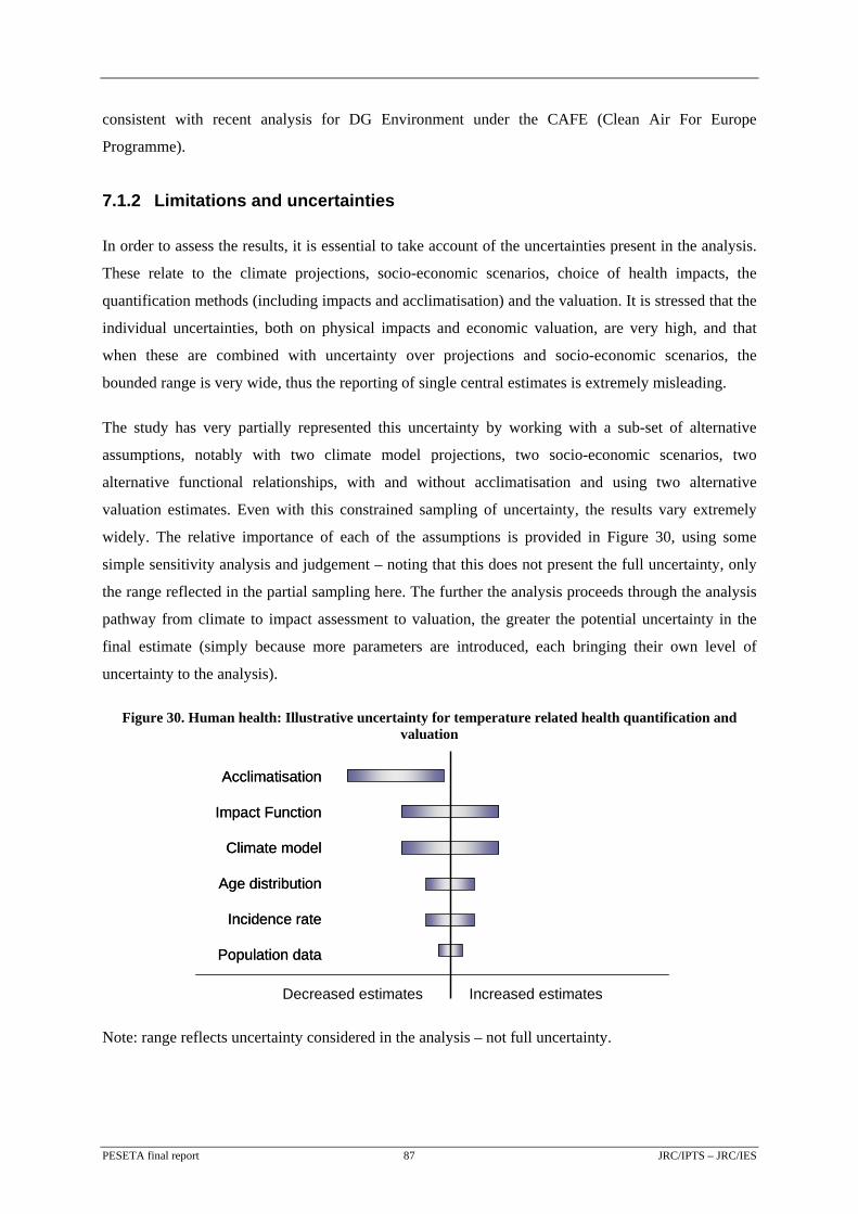
consistent with recent analysis for DG Environment under the CAFE (Clean Air For Europe
Programme).
7.1.2 Limitations and uncertainties
In order to assess the results, it is essential to take account of the uncertainties present in the analysis.
These relate to the climate projections, socio-economic scenarios, choice of health impacts, the
quantification methods (including impacts and acclimatisation) and the valuation. It is stressed that the
individual uncertainties, both on physical impacts and economic valuation, are very high, and that
when these are combined with uncertainty over projections and socio-economic scenarios, the
bounded range is very wide, thus the reporting of single central estimates is extremely misleading.
The study has very partially represented this uncertainty by working with a sub-set of alternative
assumptions, notably with two climate model projections, two socio-economic scenarios, two
alternative functional relationships, with and without acclimatisation and using two alternative
valuation estimates. Even with this constrained sampling of uncertainty, the results vary extremely
widely. The relative importance of each of the assumptions is provided in Figure 30, using some
simple sensitivity analysis and judgement – noting that this does not present the full uncertainty, only
the range reflected in the partial sampling here. The further the analysis proceeds through the analysis
pathway from climate to impact assessment to valuation, the greater the potential uncertainty in the
final estimate (simply because more parameters are introduced, each bringing their own level of
uncertainty to the analysis).
Figure 30. Human health: Illustrative uncertainty for temperature related health quantification and valuation
Acclimatisation
Impact Function
Climate model
Age distribution
Incidence rate
Population data
Acclimatisation
Impact Function
Climate model
Age distribution
Incidence rate
Population data
Increased estimatesDecreased estimates
Note: range reflects uncertainty considered in the analysis – not full uncertainty.
PESETA final report 87 JRC/IPTS – JRC/IES
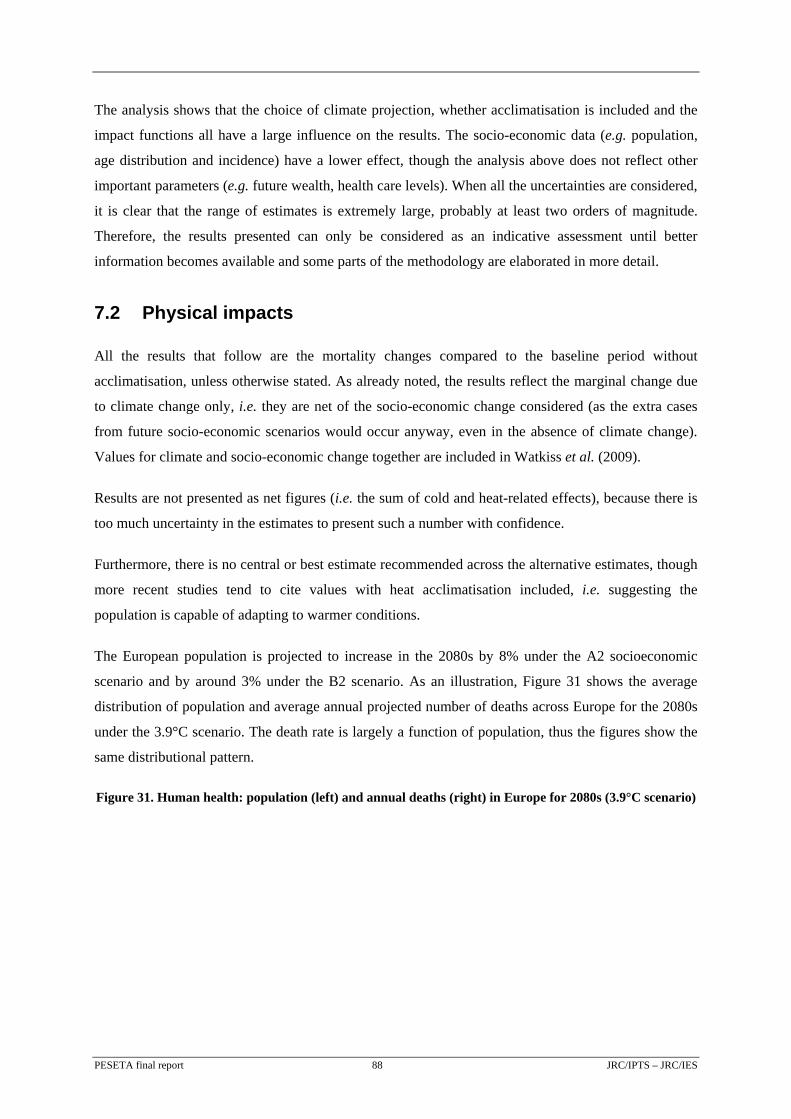
The analysis shows that the choice of climate projection, whether acclimatisation is included and the
impact functions all have a large influence on the results. The socio-economic data (e.g. population,
age distribution and incidence) have a lower effect, though the analysis above does not reflect other
important parameters (e.g. future wealth, health care levels). When all the uncertainties are considered,
it is clear that the range of estimates is extremely large, probably at least two orders of magnitude.
Therefore, the results presented can only be considered as an indicative assessment until better
information becomes available and some parts of the methodology are elaborated in more detail.
7.2 Physical impacts
All the results that follow are the mortality changes compared to the baseline period without
acclimatisation, unless otherwise stated. As already noted, the results reflect the marginal change due
to climate change only, i.e. they are net of the socio-economic change considered (as the extra cases
from future socio-economic scenarios would occur anyway, even in the absence of climate change).
Values for climate and socio-economic change together are included in Watkiss et al. (2009).
Results are not presented as net figures (i.e. the sum of cold and heat-related effects), because there is
too much uncertainty in the estimates to present such a number with confidence.
Furthermore, there is no central or best estimate recommended across the alternative estimates, though
more recent studies tend to cite values with heat acclimatisation included, i.e. suggesting the
population is capable of adapting to warmer conditions.
The European population is projected to increase in the 2080s by 8% under the A2 socioeconomic
scenario and by around 3% under the B2 scenario. As an illustration, Figure 31 shows the average
distribution of population and average annual projected number of deaths across Europe for the 2080s
under the 3.9°C scenario. The death rate is largely a function of population, thus the figures show the
same distributional pattern.
Figure 31. Human health: population (left) and annual deaths (right) in Europe for 2080s (3.9°C scenario)
PESETA final report 88 JRC/IPTS – JRC/IES
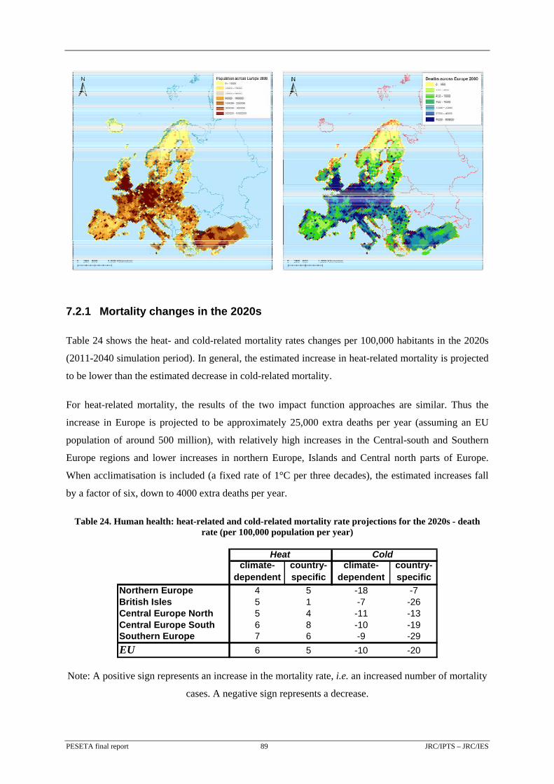
PESETA final report 89 JRC/IPTS – JRC/IES
7.2.1 Mortality changes in the 2020s
Table 24 shows the heat- and cold-related mortality rates changes per 100,000 habitants in the 2020s
(2011-2040 simulation period). In general, the estimated increase in heat-related mortality is projected
to be lower than the estimated decrease in cold-related mortality.
For heat-related mortality, the results of the two impact function approaches are similar. Thus the
increase in Europe is projected to be approximately 25,000 extra deaths per year (assuming an EU
population of around 500 million), with relatively high increases in the Central-south and Southern
Europe regions and lower increases in northern Europe, Islands and Central north parts of Europe.
When acclimatisation is included (a fixed rate of 1°C per three decades), the estimated increases fall
by a factor of six, down to 4000 extra deaths per year.
Table 24. Human health: heat-related and cold-related mortality rate projections for the 2020s - death rate (per 100,000 population per year)
climate-dependent
country-specific
climate-dependent
country-specific
Northern Europe 4 5 -18 -7British Isles 5 1 -7 -26Central Europe North 5 4 -11 -1Central Europe South 6 8 -10 -1Southern Europe 7 6 -9 -29EU 6 5 -10 -2
Heat Cold
39
0
Note: A positive sign represents an increase in the mortality rate, i.e. an increased number of mortality
cases. A negative sign represents a decrease.
Regarding cold-related mortality, the analysis projects a fall in mortality, with potentially some 50,000
to 100,000 cold-related deaths avoided. In this case the impact functions produce very different
results, varying by a factor of two. The introduction of a decline in the sensitivity of mortality to cold,
whilst only undertaken as a sensitivity, does show very large reductions in the predicted changes (i.e.
in this case much lower levels of reduced cold related deaths), with a factor of five to ten reduction
depending on the approach.
Figure 32 and Figure 33 show the 50 km x 50 km resolution maps for the heat and cold-related death
rates using the two kinds of exposure-response functions. Note that figures are not presented for the
absolute change, expressed as numbers of deaths, because these maps would be dominated by
population density, and just reflect urbanisation patterns on a 50 by 50 km resolution across Europe.
Figure 32. Human health: average annual heat-related (left) and cold-related (right) death rates per 100,000 population, for the 2020s, using the climate-dependent health functions (no acclimatisation)
PESETA final report 90 JRC/IPTS – JRC/IES
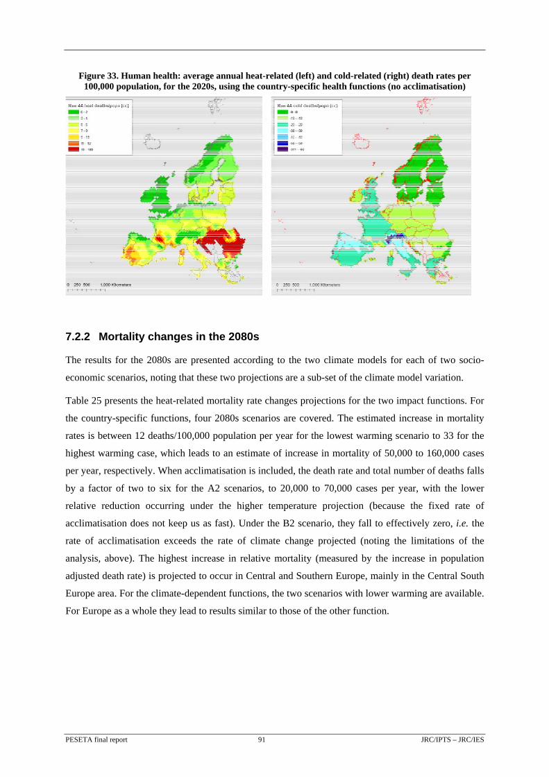
Figure 33. Human health: average annual heat-related (left) and cold-related (right) death rates per 100,000 population, for the 2020s, using the country-specific health functions (no acclimatisation)
7.2.2 Mortality changes in the 2080s
The results for the 2080s are presented according to the two climate models for each of two socio-
economic scenarios, noting that these two projections are a sub-set of the climate model variation.
Table 25 presents the heat-related mortality rate changes projections for the two impact functions. For
the country-specific functions, four 2080s scenarios are covered. The estimated increase in mortality
rates is between 12 deaths/100,000 population per year for the lowest warming scenario to 33 for the
highest warming case, which leads to an estimate of increase in mortality of 50,000 to 160,000 cases
per year, respectively. When acclimatisation is included, the death rate and total number of deaths falls
by a factor of two to six for the A2 scenarios, to 20,000 to 70,000 cases per year, with the lower
relative reduction occurring under the higher temperature projection (because the fixed rate of
acclimatisation does not keep us as fast). Under the B2 scenario, they fall to effectively zero, i.e. the
rate of acclimatisation exceeds the rate of climate change projected (noting the limitations of the
analysis, above). The highest increase in relative mortality (measured by the increase in population
adjusted death rate) is projected to occur in Central and Southern Europe, mainly in the Central South
Europe area. For the climate-dependent functions, the two scenarios with lower warming are available.
For Europe as a whole they lead to results similar to those of the other function.
PESETA final report 91 JRC/IPTS – JRC/IES
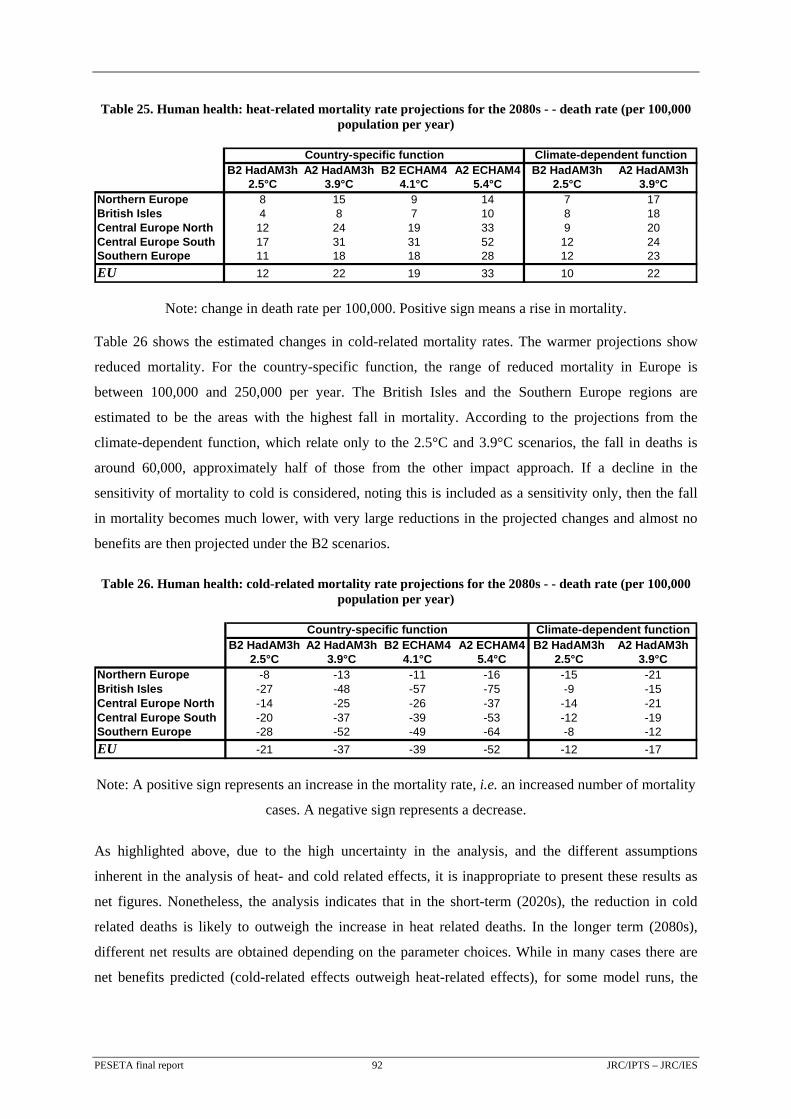
Table 25. Human health: heat-related mortality rate projections for the 2080s - - death rate (per 100,000 population per year)
B2 HadAM3h A2 HadAM3h B2 ECHAM4 A2 ECHAM4 B2 HadAM3h A2 HadAM3h2.5°C 3.9°C 4.1°C 5.4°C 2.5°C 3.9°C
Northern Europe 8 15 9 14 7 17British Isles 4 8 7 10 8 18Central Europe North 12 24 19 33 9 20Central Europe South 17 31 31 52 12 24Southern Europe 11 18 18 28 12 23EU 12 22 19 33 10 22
Country-specific function Climate-dependent function
Note: change in death rate per 100,000. Positive sign means a rise in mortality.
Table 26 shows the estimated changes in cold-related mortality rates. The warmer projections show
reduced mortality. For the country-specific function, the range of reduced mortality in Europe is
between 100,000 and 250,000 per year. The British Isles and the Southern Europe regions are
estimated to be the areas with the highest fall in mortality. According to the projections from the
climate-dependent function, which relate only to the 2.5°C and 3.9°C scenarios, the fall in deaths is
around 60,000, approximately half of those from the other impact approach. If a decline in the
sensitivity of mortality to cold is considered, noting this is included as a sensitivity only, then the fall
in mortality becomes much lower, with very large reductions in the projected changes and almost no
benefits are then projected under the B2 scenarios.
Table 26. Human health: cold-related mortality rate projections for the 2080s - - death rate (per 100,000 population per year)
B2 HadAM3h A2 HadAM3h B2 ECHAM4 A2 ECHAM4 B2 HadAM3h A2 HadAM3h2.5°C 3.9°C 4.1°C 5.4°C 2.5°C 3.9°C
Northern Europe -8 -13 -11 -16 -15 -21British Isles -27 -48 -57 -75 -9 -15Central Europe North -14 -25 -26 -37 -14 -21Central Europe South -20 -37 -39 -53 -12 -19Southern Europe -28 -52 -49 -64 -8 -12EU -21 -37 -39 -52 -12 -17
Country-specific function Climate-dependent function
Note: A positive sign represents an increase in the mortality rate, i.e. an increased number of mortality
cases. A negative sign represents a decrease.
As highlighted above, due to the high uncertainty in the analysis, and the different assumptions
inherent in the analysis of heat- and cold related effects, it is inappropriate to present these results as
net figures. Nonetheless, the analysis indicates that in the short-term (2020s), the reduction in cold
related deaths is likely to outweigh the increase in heat related deaths. In the longer term (2080s),
different net results are obtained depending on the parameter choices. While in many cases there are
net benefits predicted (cold-related effects outweigh heat-related effects), for some model runs, the
PESETA final report 92 JRC/IPTS – JRC/IES
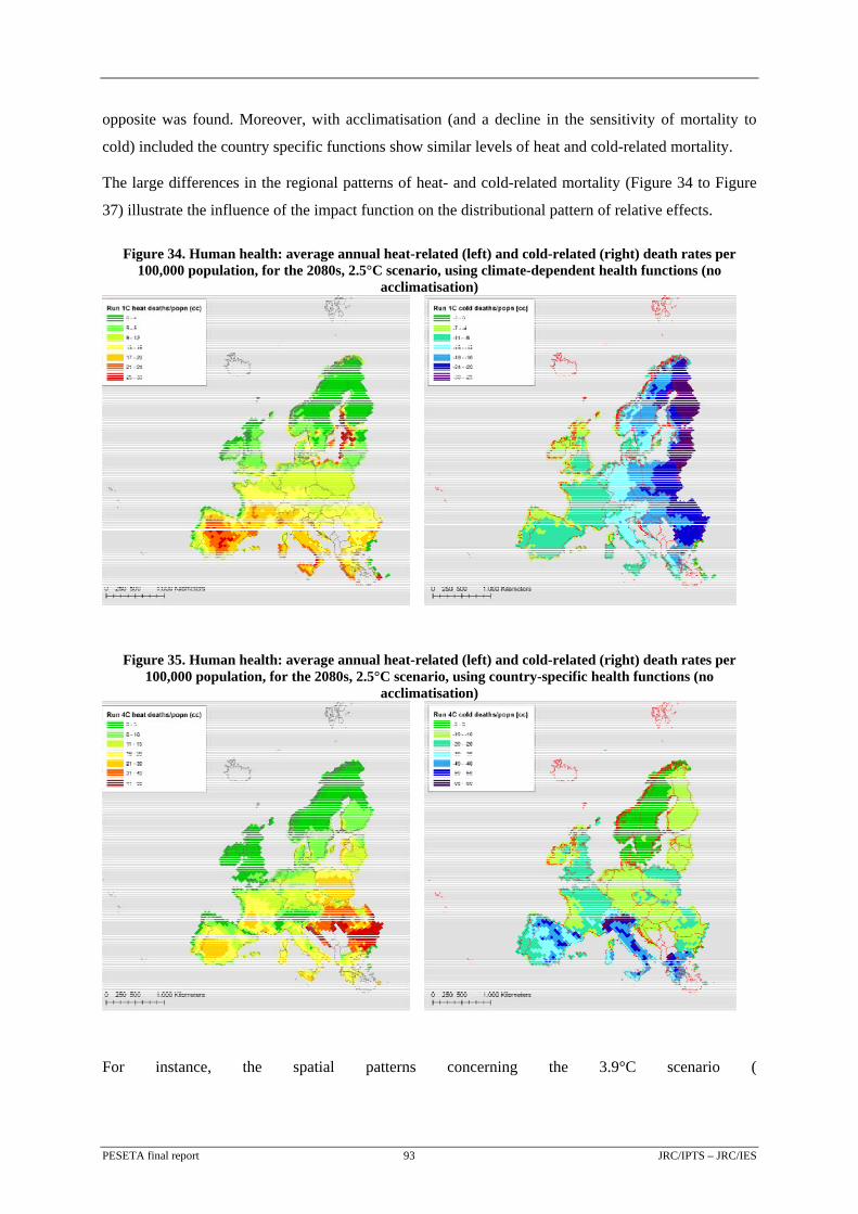
opposite was found. Moreover, with acclimatisation (and a decline in the sensitivity of mortality to
cold) included the country specific functions show similar levels of heat and cold-related mortality.
The large differences in the regional patterns of heat- and cold-related mortality (Figure 34 to Figure
37) illustrate the influence of the impact function on the distributional pattern of relative effects.
Figure 34. Human health: average annual heat-related (left) and cold-related (right) death rates per 100,000 population, for the 2080s, 2.5°C scenario, using climate-dependent health functions (no
acclimatisation)
Figure 35. Human health: average annual heat-related (left) and cold-related (right) death rates per 100,000 population, for the 2080s, 2.5°C scenario, using country-specific health functions (no
acclimatisation)
For instance, the spatial patterns concerning the 3.9°C scenario (
PESETA final report 93 JRC/IPTS – JRC/IES
Figure 36 and Figure 37) show that for heat related mortality:
• With the climate dependent functions, the pattern is relatively uniform across Member States,
though the largest potential mortality increases from climate change occur in Mediterranean and
south-eastern European countries and the smallest potential increases in more northerly and north-
west countries. This reflects the relative level of warming projected in the models, because this
approach uses a consistent slope function (though different thresholds) and so more closely
reflects climate parameters.
• With the country specific functions, there is more variability between Member States, reflecting
the larger difference in the underlying functions derived from individual country studies. Central-
eastern countries show the strongest climate change induced increases, reflecting the higher
gradients in the functions for these regions.
The spatial patterns show that for cold related mortality:
• With the climate dependent functions, the largest potential cold-mortality benefits from climate
change occur in Baltic and Scandinavian countries, while the smallest benefits are found in
Ireland, Luxembourg, UK and some Mediterranean countries – again matching the underlying
pattern from the climate model projections.
• With the country specific functions, the largest potential cold-mortality benefits from climate
change occur mainly in Mediterranean countries, reflecting the relative slope of the functions,
while the smallest benefits are in Baltic and Scandinavian countries.
PESETA final report 94 JRC/IPTS – JRC/IES

Figure 36. Human health: average annual heat-related (left) and cold-related (right) death rates per 100,000 population for the 2080s, 3.9°C scenario, using climate-dependent health functions (no
acclimatisation)
Figure 37. Human health: average annual heat-related (left) and cold-related (right) death rates per 100,000 population for the 2080s, 3.9°C scenario, using country-specific health functions (no
acclimatisation)
An overview of all the physical impacts is provided in Figure 38.
PESETA final report 95 JRC/IPTS – JRC/IES
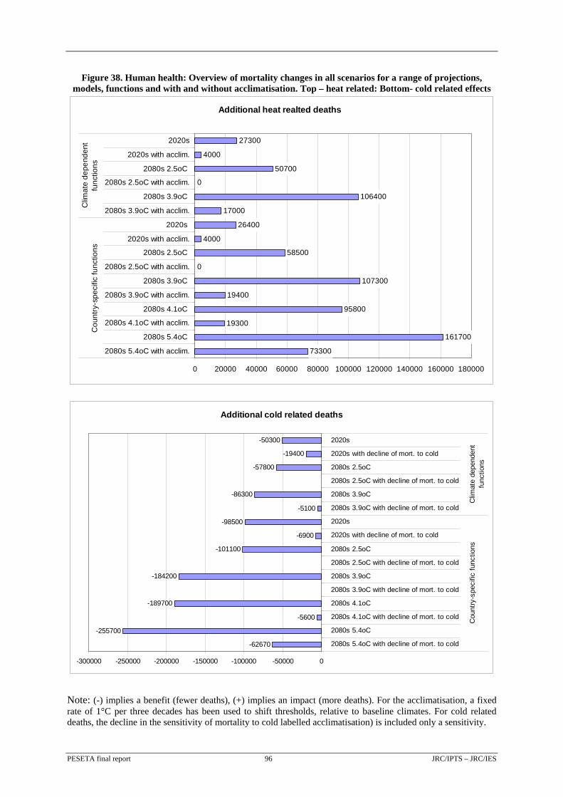
Figure 38. Human health: Overview of mortality changes in all scenarios for a range of projections, models, functions and with and without acclimatisation. Top – heat related: Bottom- cold related effects
Additional heat realted deaths
73300
161700
19300
95800
19400
107300
0
58500
4000
26400
17000
106400
0
50700
4000
27300
0 20000 40000 60000 80000 100000 120000 140000 160000 180000
2080s 5.4oC with acclim.
2080s 5.4oC
2080s 4.1oC with acclim.
2080s 4.1oC
2080s 3.9oC with acclim.
2080s 3.9oC
2080s 2.5oC with acclim.
2080s 2.5oC
2020s with acclim.
2020s
2080s 3.9oC with acclim.
2080s 3.9oC
2080s 2.5oC with acclim.
2080s 2.5oC
2020s with acclim.
2020s
Cou
ntry
-spe
cific
func
tions
Clim
ate
depe
nden
tfu
nctio
ns
Additional cold related deaths
-62670
-255700
-5600
-189700
-184200
-101100
-6900
-98500
-5100
-86300
-57800
-19400
-50300
0
0
0
-300000 -250000 -200000 -150000 -100000 -50000 0
2080s 5.4oC with decline of mort. to cold
2080s 5.4oC
2080s 4.1oC with decline of mort. to cold
2080s 4.1oC
2080s 3.9oC with decline of mort. to cold
2080s 3.9oC
2080s 2.5oC with decline of mort. to cold
2080s 2.5oC
2020s with decline of mort. to cold
2020s
2080s 3.9oC with decline of mort. to cold
2080s 3.9oC
2080s 2.5oC with decline of mort. to cold
2080s 2.5oC
2020s with decline of mort. to cold
2020s
Cou
ntry
-spe
cific
func
tions
Clim
ate
depe
nden
tfu
nctio
ns
Note: (-) implies a benefit (fewer deaths), (+) implies an impact (more deaths). For the acclimatisation, a fixed rate of 1°C per three decades has been used to shift thresholds, relative to baseline climates. For cold related deaths, the decline in the sensitivity of mortality to cold labelled acclimatisation) is included only a sensitivity.
PESETA final report 96 JRC/IPTS – JRC/IES
7.3 Economic impacts
Table 27 shows the results for all cases according to the two valuation methods. In general the
monetary values follow the pattern of physical impacts above and so no additional detailed description
is included here. Heat and cold related annual effects are valued in terms of tens to hundreds of
billions of Euros.
For the 2020s without acclimatisation, the heat-related effects are valued at 13 billion € when applying
the VOLY method and at 30 billion € applying the VSL approach (assuming that on average, eight
years of life is lost per case), though drop to 2 to 4 billion €when acclimatisation is included. For the
results presented here, values are provided in constant values (year 2005, no uplift, no discounting) to
allow direct comparison across periods. The benefit due to the reduction of cold-related deaths are
valued at 23 to 46 billion € according to the VOLY method and 55 to 110 billion € with the VSL
method, though again these become less significant if a decline in the sensitivity of mortality to cold is
included (note again that the same period of life lost is assumed for the VOLY, though different
periods of life are likely to be lost, on average, for heat- and cold-related mortality).
By 2100 under an A2 projection, the values range from 50 to 180 billion Euro (according to choice of
function and climate model) without acclimatisation, and 8 to 80 billion Euro/year with
acclimatisation. Similar or higher benefits are projected for the reduction in cold-related mortality. In
respect of valuation, some additional points emerge. The choice of valuation metric (VOLY or VSL)
is important, as is the period of life lost that is assumed for mortality (when using the VOLY). The
choice of VOLY or VSL metric leads to a factor of 2 to 3 difference (with higher estimates when
applying VSL values). This adds to uncertainty additional to that already highlighted above.
Because of the uncertainties, we caution against the reporting of net economic effects. Nevertheless,
whilst noting the caveats above in relation to the sum of heat- and cold-related effects, the results show
that depending on the parameter choices, the benefits from the reduction in cold-related deaths are
usually at least as large, and under many scenarios, larger than the increase in heat-related deaths.
However, the results here exclude additional effects from heatwaves. More importantly, for many the
other health categories covered in the main report, i.e. temperature-related cases of salmonella, flood
related heath effects, there are no positive related effects from climate change, only impacts.
PESETA final report 97 JRC/IPTS – JRC/IES
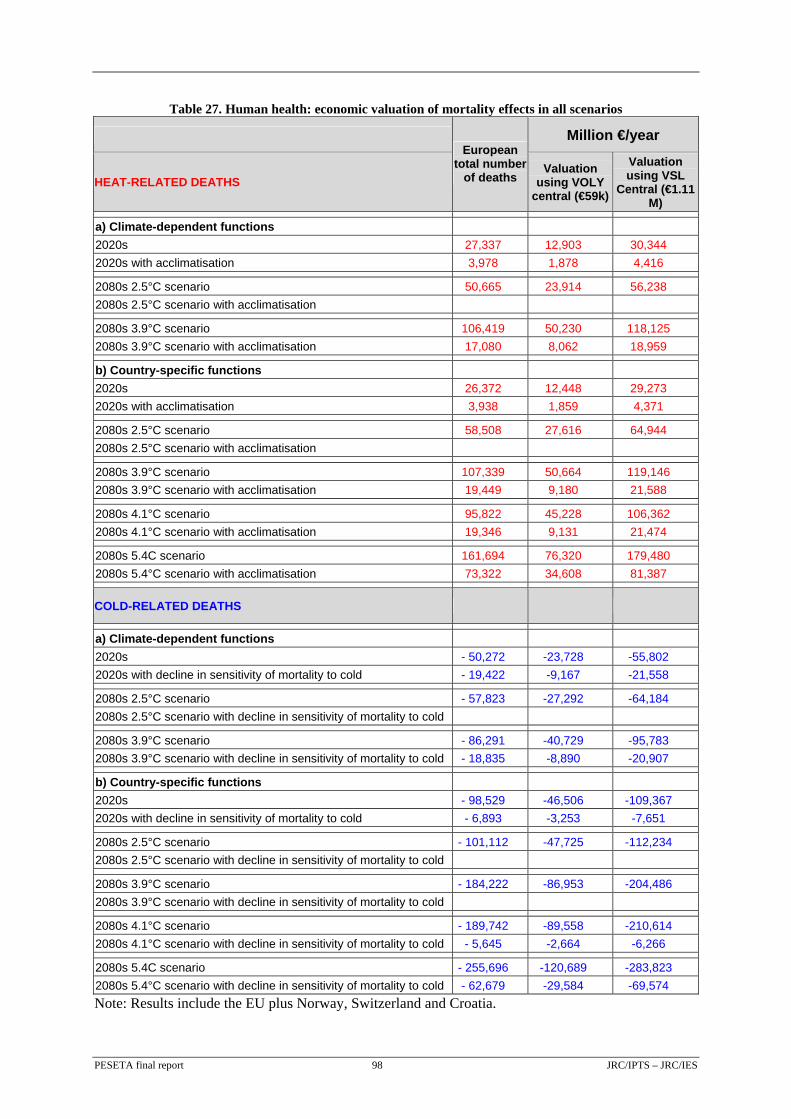
PESETA final report 98 JRC/IPTS – JRC/IES
Table 27. Human health: economic valuation of mortality effects in all scenarios
Million €/year
HEAT-RELATED DEATHS
European total number
of deaths Valuation
using VOLY central (€59k)
Valuation using VSL
Central (€1.11 M)
a) Climate-dependent functions 2020s 27,337 12,903 30,344 2020s with acclimatisation 3,978 1,878 4,416
2080s 2.5°C scenario 50,665 23,914 56,238 2080s 2.5°C scenario with acclimatisation
2080s 3.9°C scenario 106,419 50,230 118,125 2080s 3.9°C scenario with acclimatisation 17,080 8,062 18,959
b) Country-specific functions 2020s 26,372 12,448 29,273 2020s with acclimatisation 3,938 1,859 4,371
2080s 2.5°C scenario 58,508 27,616 64,944 2080s 2.5°C scenario with acclimatisation
2080s 3.9°C scenario 107,339 50,664 119,146 2080s 3.9°C scenario with acclimatisation 19,449 9,180 21,588
2080s 4.1°C scenario 95,822 45,228 106,362 2080s 4.1°C scenario with acclimatisation 19,346 9,131 21,474
2080s 5.4C scenario 161,694 76,320 179,480 2080s 5.4°C scenario with acclimatisation 73,322 34,608 81,387
COLD-RELATED DEATHS
a) Climate-dependent functions 2020s - 50,272 -23,728 -55,802 2020s with decline in sensitivity of mortality to cold - 19,422 -9,167 -21,558
2080s 2.5°C scenario - 57,823 -27,292 -64,184 2080s 2.5°C scenario with decline in sensitivity of mortality to cold
2080s 3.9°C scenario - 86,291 -40,729 -95,783 2080s 3.9°C scenario with decline in sensitivity of mortality to cold - 18,835 -8,890 -20,907
b) Country-specific functions 2020s - 98,529 -46,506 -109,367 2020s with decline in sensitivity of mortality to cold - 6,893 -3,253 -7,651
2080s 2.5°C scenario - 101,112 -47,725 -112,234 2080s 2.5°C scenario with decline in sensitivity of mortality to cold
2080s 3.9°C scenario - 184,222 -86,953 -204,486 2080s 3.9°C scenario with decline in sensitivity of mortality to cold
2080s 4.1°C scenario - 189,742 -89,558 -210,614 2080s 4.1°C scenario with decline in sensitivity of mortality to cold - 5,645 -2,664 -6,266
2080s 5.4C scenario - 255,696 -120,689 -283,823 2080s 5.4°C scenario with decline in sensitivity of mortality to cold - 62,679 -29,584 -69,574 Note: Results include the EU plus Norway, Switzerland and Croatia.

8 INTEGRATED ECONOMIC ASSESSMENT OF MARKET IMPACTS: THE GEM-E3 PESETA MODEL
8.1 Introduction
The physical and economic results of the four market impact categories of the PESETA project (i.e.
agriculture, river floods, coastal systems, and tourism) have been integrated into the computable
general equilibrium (CGE) GEM-E3 Europe model in order to have a comparable vision of impacts
across sectors. The ultimate purpose of this preliminary analysis has been to get insights on which
aspects of the European economy and which geographical areas are more vulnerable to climate
change, without considering public adaptation.
In other words, the aim has been to explore where and why climate change matters in Europe
potentially, so that the results can shed some light in prioritizing adaptation in Europe across sectors
and countries, a clear policy need as noted in the White Paper on Adaptation (European Commission,
2009a).
The four scenarios for the 2080s, common to all sectoral studies, have been considered (Section 2.3.4),
named after the average increase in temperature in the EU, compared to the 1961-1990 period: 2.5°C,
3.9°C, 4.1°C, and 5.4°C.
Given the limited sectoral scope of the PESETA project, other sectors and impact might as well
matter. From this point of view, the results of this analysis need to be interpreted carefully. This
chapter presents the main elements of the methodology and the key results.
8.2 Methodology of integration
Figure 39 indicates the various stages of the research project. The rectangles symbolize models and the
circles input data or numerical results. The first stage is the modelling of climate futures. The selected
socioeconomic scenarios make assumptions on the drivers of climate change i.e. economic growth and
population dynamics. The resulting greenhouse gas (GHG) emissions are the input to the climate
models, which yield the climate variables (Section 2.3).
PESETA final report 99 JRC/IPTS – JRC/IES
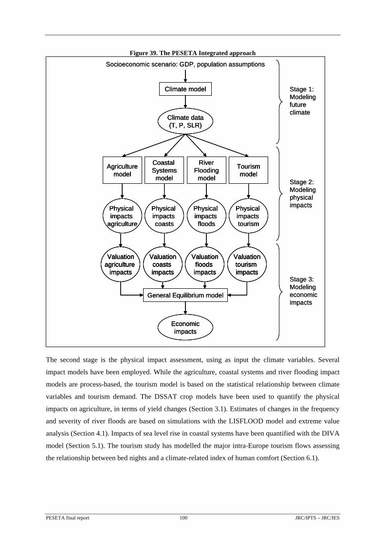
Figure 39. The PESETA Integrated approach
Socioeconomic scenario: GDP, population assumptions
Agriculturemodel
Coastal Systems
model
RiverFlooding
model
Tourismmodel
Stage 1:Modelingfuture climate
Physical impacts
agriculture
Physical impacts coasts
Physical impacts floods
Physical impacts tourism
Stage 2:Modelingphysicalimpacts
Stage 3:Modelingeconomicimpacts
Climate model
General Equilibrium model
Climate data(T, P, SLR)
Economicimpacts
Valuationagriculture
impacts
Valuationcoasts impacts
Valuationfloods impacts
Valuationtourism impacts
Socioeconomic scenario: GDP, population assumptions
Agriculturemodel
Coastal Systems
model
RiverFlooding
model
Tourismmodel
Agriculturemodel
Coastal Systems
model
RiverFlooding
model
Tourismmodel
Stage 1:Modelingfuture climate
Physical impacts
agriculture
Physical impacts coasts
Physical impacts floods
Physical impacts tourism
Physical impacts
agriculture
Physical impacts coasts
Physical impacts floods
Physical impacts tourism
Stage 2:Modelingphysicalimpacts
Stage 3:Modelingeconomicimpacts
Climate model
General Equilibrium model
Climate data(T, P, SLR)
Economicimpacts
Climate model
General Equilibrium model
Climate data(T, P, SLR)
Economicimpacts
Valuationagriculture
impacts
Valuationcoasts impacts
Valuationfloods impacts
Valuationtourism impacts
Valuationagriculture
impacts
Valuationcoasts impacts
Valuationfloods impacts
Valuationtourism impacts
Valuationagriculture
impacts
Valuationcoasts impacts
Valuationfloods impacts
Valuationtourism impacts
The second stage is the physical impact assessment, using as input the climate variables. Several
impact models have been employed. While the agriculture, coastal systems and river flooding impact
models are process-based, the tourism model is based on the statistical relationship between climate
variables and tourism demand. The DSSAT crop models have been used to quantify the physical
impacts on agriculture, in terms of yield changes (Section 3.1). Estimates of changes in the frequency
and severity of river floods are based on simulations with the LISFLOOD model and extreme value
analysis (Section 4.1). Impacts of sea level rise in coastal systems have been quantified with the DIVA
model (Section 5.1). The tourism study has modelled the major intra-Europe tourism flows assessing
the relationship between bed nights and a climate-related index of human comfort (Section 6.1).
PESETA final report 100 JRC/IPTS – JRC/IES

The third stage relates to the evaluation of the direct and indirect economic effects of the physical
impacts. A multi-sector CGE model for Europe, the GEM-E3 Europe model, has been run to assess
the effects of the various impacts on consumer welfare and GDP. Multi-country CGE models provide
an explicit treatment of the interactions between different economic sectors and markets (production
factors and goods and services), while taking into account the trade flows between countries. This
framework captures not only the direct effects of a particular climate impact but also the indirect
effects in the rest of the economy. The CGE model ultimately translates the climate change scenarios
into consumer welfare and GDP changes, compared to the baseline scenario.
8.3 Effect of 2080s climate in the current economy
The assessment evaluates the economic effects of future climate change (projected for the 2080s) on
the current economy, as of 2010. Several authors have followed this approach (e.g. Fankhauser and
Tol, 1996; Halsnæs et al., 2007). This static analysis would be the equivalent of having the 2080s
climate in today's economy.
The alternative approach, followed e.g. in Bosello et al. (2007), would be to model the effect of future
climate in the future economy. Implementing a static approach has the advantage that assumptions on
the future evolution of the economy over the next eight decades are not introduced, minimizing the
number of assumptions, and, moreover, that the interpretation of the results becomes simpler and more
understandable. Impacts are also presented undiscounted. Time discounting is a key and controversial
issue in evaluating the impacts of climate change (Nordhaus, 2007; Stern and Taylor, 2007).
A baseline scenario has been run for 2010. The alternative scenario considered the influence of climate
change in the economy. The results of the CGE analysis compare the values of welfare and GDP of
the climate scenario to those of the baseline scenario.
8.4 Potential impacts and adaptation
Potential impacts of climate change are defined by the IPCC as 'all impacts that may occur given a
projected change in climate, without considering adaptation' (IPCC, 2007b; Levina and Tirpak, 2006).
The assessment of potential impacts in various sectors facilitates the identification of priorities in
adaptation policies.
In the various models applied in this analysis only private adaptation actions have been taken into
account (e.g. farm level adaptation, change in tourism flows, migration to safer areas) but no explicit
public adaptation policy has been considered. While the DIVA model uses a more sophisticated cost-
benefit framework (Tol, 2005) to determine the optimal level of adaptation, in this assessment this
option has been disabled in order to measure the potential impact of SLR, as for the other impact
categories.
PESETA final report 101 JRC/IPTS – JRC/IES
8.5 Overview of physical impacts
Table 28 presents the main physical impacts for the impact studies. Regarding agriculture, Southern
Europe would experience yield losses, which would become relatively high for the 5.4°C scenario.
Central Europe regions would have moderate yield changes. The Northern Europe region would
benefit from positive yield changes in all scenarios, and to a lesser extent the British Isles for the 4.1°C
and 5.4°C scenarios.
River flooding would affect 250,000 to 400,000 additional people per year in Europe by the 2080s,
more than doubling the number with respect to the 1961–1990 period. In coastal areas, around one
million additional people would be subject to flooding every year due to SLR. For the highest SLR
scenario (88 cm), an additional 5.5 million people per year are exposed to flooding in the EU.
For tourism, climate change would induce better conditions for most regions, resulting in more bed
nights and inducing a relatively small EU-wide positive impact. Southern Europe, which currently
accounts for more than half of the total EU capacity of tourist accommodation, would be the only
region with a decline in bed nights.
PESETA final report 102 JRC/IPTS – JRC/IES
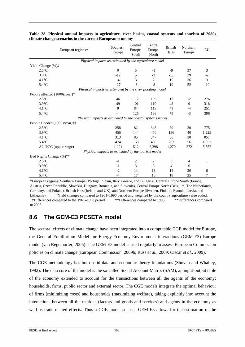
Table 28. Physical annual impacts in agriculture, river basins, coastal systems and tourism of 2080s climate change scenarios in the current European economy
European regions* Southern Europe
Central Europe South
Central Europe North
British Isles
Northern Europe EU
Yield Change (%)‡2.5°C 0 5 -1 -9 37 33.9°C -12 5 -3 -11 39 -24.1°C -4 3 2 15 36 35.4°C -27 -3 -8 19 52 -10
People affected (1000s/year)†2.5°C 46 117 103 12 -2 2763.9°C 49 101 110 48 9 3184.1°C 9 84 119 43 -4 2515.4°C -4 125 198 79 -3 396
People flooded (1000s/year)††2.5°C 258 82 345 70 20 7753.9°C 456 144 450 136 40 1,2254.1°C 313 85 347 86 20 8515.4°C 474 158 459 207 56 1,353A2 IPCC (upper range) 1,091 512 2,398 1,279 272 5,552
Bed Nights Change (%)**2.5°C -1 2 2 3 4 13.9°C -1 3 3 4 6 14.1°C -2 14 13 14 20 65.4°C -4 17 16 18 25 7
Physical impacts as estimated by the agriculture model
Physical impacts as estimated by the coastal systems model
*European regions: Southern Europe (Portugal, Spain, Italy, Greece, and Bulgaria), Central Europe South (France, Austria, Czech Republic, Slovakia, Hungary, Romania, and Slovenia), Central Europe North (Belgium, The Netherlands, Germany, and Poland), British Isles (Ireland and UK), and Northern Europe (Sweden, Finland, Estonia, Latvia, and Lithuania). ‡Yield changes compared to 1961–1990 period and weighted by the country agriculture value added. †Differences compared to the 1961–1990 period. ††Differences compared to 1995. **Differences compared to 2005.
Physical impacts as estimated by the tourism model
Physical impacts as estimated by the river flooding model
8.6 The GEM-E3 PESETA model
The sectoral effects of climate change have been integrated into a computable CGE model for Europe,
the General Equilibrium Model for Energy-Economy-Environment interactions (GEM-E3) Europe
model (van Regemorter, 2005). The GEM-E3 model is used regularly to assess European Commission
policies on climate change (European Commission, 2009b; Russ et al., 2009; Ciscar et al., 2009).
The CGE methodology has both solid data and economic theory foundations (Shoven and Whalley,
1992). The data core of the model is the so-called Social Account Matrix (SAM), an input-output table
of the economy extended to account for the transactions between all the agents of the economy:
households, firms, public sector and external sector. The CGE models integrate the optimal behaviour
of firms (minimizing costs) and households (maximizing welfare), taking explicitly into account the
interactions between all the markets (factors and goods and services) and agents in the economy as
well as trade-related effects. Thus a CGE model such as GEM-E3 allows for the estimation of the
PESETA final report 103 JRC/IPTS – JRC/IES
direct and indirect effects of climate change in the overall economy. The direct effect on a sector
would lead to indirect effects in the rest of the goods and services markets through adjustments in the
factor markets (capital and labour markets) and in trade to attain equilibrium between supply and
demand in all markets.
The GEM-E3 economic, energy and emissions data are based on EUROSTAT databases (input-output
tables, national accounts data and energy balances). Twenty-four EU economies haven been
individually modelled (the whole EU with the exception of Malta, Cyprus and Luxemburg), with
eighteen sectors in each country with full bilateral trade.
As a benchmark it has been assumed that all markets are fully flexible, i.e. prices in all markets adjust
so that demand equals supply. Such a neoclassical paradigm has been used to represent the new
equilibrium in the long-term when all market adjustments have occurred. This framework is assumed
in many integrated assessment models (e.g. Nordhaus, 1994).
8.7 Integration of impacts into the GEM-E3 PESETA Model
Each impact category has been modelled differently in the GEM-E3 model, depending on the
interpretation of the direct effect.
The yield changes computed with the agriculture model have been interpreted as a productivity shock
to the production side of the agriculture sector in the economy.
The main economic impacts of river flooding relate to damages in residential buildings (around 80%
of the total impact). It has been assumed that households would repair buildings and replace lost
equipment. This is interpreted as additional expenditure needed. The damages related to productive
sectors are modelled as production and capital losses in the economy, representing only 20% of the
damage from flood and thus only marginally affecting GDP.
In the coastal system assessment, the two main economic impacts estimated by the DIVA model are
sea floods and migration costs. It has been assumed that sea floods lead to capital losses, while
migration costs induce additional expenditure by households. For both river floods and coastal
systems, this additional expenditure does not provide any welfare gain: it represents indeed a welfare
loss, since households are forced to it due to climate change.
For tourism, it has been assumed that the redistribution of tourism within Europe leads to changes in
exports; some countries have more international tourists that lead to higher expenditure within the
country in the form of additional exports but leading also to reaction on the supply capacity. The
reported results in tourism refer to the year 2040 in order to allow the model to adjust to the new
export flows of the sector.
PESETA final report 104 JRC/IPTS – JRC/IES
GDP and welfare have selected as the main variables to synthesize the economic impact. Welfare in
CGE models measures the utility derived from household consumption and leisure time. Its evolution
reflects the benefits for households from growth, while GDP growth reflects more the domestic
economic activity growth. In the long-term reference scenario both indicators would evolve in parallel,
but policies or climate change damage might induce some activity growth without generating welfare
improvements (e.g. repairing houses after floods). The results of this study show that a significant
share of welfare increase could be eroded by climate change induced damages (0.2%-1% annual
losses).
8.8 Economic Impact Results
The consequences of climate change of the four impact categories can be valued in monetary or
economic terms as they directly affect markets and, via the cross-sector linkages, the overall economy.
The impacts of climate change affect GDP and the consumption behaviour of households, and
therefore the welfare of households. Many economic impact assessments focus on the impacts on
GDP. However, in the framework of the PESETA project the impact of climate change on household
welfare seems the most appropriate metric to measure the influence of climate change on the economy
for two reasons. Firstly, in CGE models (i.e. the GEM-E3 model) households usually maximise their
utility or welfare level and not GDP. From this point of view, welfare changes give an indication of
the deviation from the optimum situation the household would achieve without climate change (the
reference scenario). GDP can be rather interpreted as a measure of the adjustment in the production or
supply-side of the economy because of climate change.
A second reason to employ welfare changes rather than GDP is the way the climate sectoral shocks
have been interpreted and implemented into the CGE GEM-E3 model. Indeed, while some impact
categories (e.g. agriculture) have a direct effect on the production side of the economic system, other
impacts, notably the damages due to floods, affect mainly the consumption possibilities of households
and, therefore, household welfare, with and indirect effect on production activities.
The next subsections summarise the main results in welfare and GDP terms.
8.8.1 Welfare effects of climate change in Europe
Table 29 presents the annual welfare changes by European region for the five climate futures
considered in the 2080s: the four 2080s scenarios plus a the 5.4°C scenario with the highest range of
SLR of the IPCC (88 cm). Figure 40 presents the same information with the sectoral breakdown.
PESETA final report 105 JRC/IPTS – JRC/IES
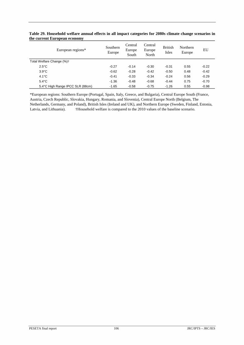
Table 29. Household welfare annual effects in all impact categories for 2080s climate change scenarios in the current European economy
European regions* Southern Europe
Central Europe South
Central Europe North
British Isles
Northern Europe EU
Total Welfare Change (%)†2.5°C -0.27 -0.14 -0.30 -0.31 0.55 -0.223.9°C -0.62 -0.28 -0.42 -0.50 0.48 -0.424.1°C -0.41 -0.33 -0.34 -0.24 0.56 -0.295.4°C -1.36 -0.48 -0.68 -0.44 0.75 -0.705.4°C High Range IPCC SLR (88cm) -1.65 -0.58 -0.75 -1.26 0.55 -0.98
*European regions: Southern Europe (Portugal, Spain, Italy, Greece, and Bulgaria), Central Europe South (France, Austria, Czech Republic, Slovakia, Hungary, Romania, and Slovenia), Central Europe North (Belgium, The Netherlands, Germany, and Poland), British Isles (Ireland and UK), and Northern Europe (Sweden, Finland, Estonia, Latvia, and Lithuania). †Household welfare is compared to the 2010 values of the baseline scenario.
PESETA final report 106 JRC/IPTS – JRC/IES
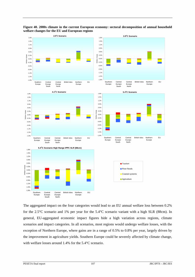
Figure 40. 2080s climate in the current European economy: sectoral decomposition of annual household welfare changes for the EU and European regions 2.5oC Scenario
-1.8%
-1.5%
-1.2%
-0.9%
-0.6%
-0.3%
0.0%
0.3%
0.6%
0.9%
1.2%
1.5%
1.8%
SouthernEurope
CentralEuropeSouth
CentralEuropeNorth
British Isles NorthernEurope
EU
Wel
fare
cha
nge
3.9oC Scenario
-1.8%
-1.5%
-1.2%
-0.9%
-0.6%
-0.3%
0.0%
0.3%
0.6%
0.9%
1.2%
1.5%
1.8%
SouthernEurope
CentralEuropeSouth
CentralEuropeNorth
British Isles NorthernEurope
EU
Wel
fare
cha
nge
4.1oC Scenario
-1.8%
-1.5%
-1.2%
-0.9%
-0.6%
-0.3%
0.0%
0.3%
0.6%
0.9%
1.2%
1.5%
1.8%
SouthernEurope
CentralEuropeSouth
CentralEuropeNorth
British Isles NorthernEurope
EU
Wel
fare
cha
nge
5.4oC Scenario
-1.8%
-1.5%
-1.2%
-0.9%
-0.6%
-0.3%
0.0%
0.3%
0.6%
0.9%
1.2%
1.5%
1.8%
SouthernEurope
CentralEuropeSouth
CentralEuropeNorth
British Isles NorthernEurope
EU
Wel
fare
cha
nge
5.4oC Scenario High Range IPPC SLR (88cm)
-1.8%
-1.5%
-1.2%
-0.9%
-0.6%
-0.3%
0.0%
0.3%
0.6%
0.9%
1.2%
1.5%
1.8%
SouthernEurope
CentralEuropeSouth
CentralEuropeNorth
British Isles NorthernEurope
EU
Wel
fare
cha
nge
-1 .8%
-1 .5%
-1 .2%
-0.9%
-0.6%
-0.3%
0.0%
0.3%
0.6%
0.9%
1 .2%
1 .5%
1 .8%
So uthe rn Europ e Cen tral Eu rope Sou th Cen tral Eu rope North British Isle s No rthern Euro pe EU
Tourism
River floods
Coastal systems
Agriculture
The aggregated impact on the four categories would lead to an EU annual welfare loss between 0.2%
for the 2.5°C scenario and 1% per year for the 5.4°C scenario variant with a high SLR (88cm). In
general, EU-aggregated economic impact figures hide a high variation across regions, climate
scenarios and impact categories. In all scenarios, most regions would undergo welfare losses, with the
exception of Northern Europe, where gains are in a range of 0.5% to 0.8% per year, largely driven by
the improvement in agriculture yields. Southern Europe could be severely affected by climate change,
with welfare losses around 1.4% for the 5.4°C scenario.
PESETA final report 107 JRC/IPTS – JRC/IES
The sectoral and geographical decomposition of welfare changes under the 2.5°C and the 3.9°C
scenarios shows that aggregated European costs of climate change are highest for agriculture, river
flooding and coastal systems, much larger than for tourism. The British Isles, Central Europe North
and Southern Europe appear the most sensitive areas. Moreover, moving from a European climate
future of 2.5°C to one of 3.9°C aggravates agriculture impacts, river flooding potential and coastal
systems impacts in almost all European regions. In the Northern Europe area, these impacts are offset
by the increasingly positive effects related to agriculture.
The 5.4°C scenario leads to an annual EU welfare loss of 0.7%, with more pronounced impacts in
most sectors in all EU regions and a non-linear response of damages to rising temperature. The
agriculture sector is the most important impact category in the EU average: the significant damages in
Southern Europe and Central Europe South are not compensated by the gains in Northern Europe.
Impacts from river flooding are also more important in this case than in the other scenarios, with
particular aggravation in the British Isles and Central Europe. In the 5.4°C scenario variant with the
high SLR (88 cm), damages in coastal regions would become the most important impact category in
the EU, especially in the British Isles.
8.8.2 GDP effects
The impact of climate change in GDP terms is estimated to be in a range between 0.2 and 0.5% for the
EU depending on the climate scenario (Table 30), which would mean between 20 billion € for the
2.5°C scenario and 65 billion € for the 5.4°C scenario with high SLR. EU-wide production impacts
due to river floods would be minor, around 0.1% GDP loss, mainly because most of the damage would
be to residential buildings, i.e. welfare of households. Tourism impacts would also be very low in the
EU, being between -0.1% and -0.03% in the Southern Europe region and for a similar range across all
European regions in the 5.4°C scenario.
Agriculture-related productive impacts would be negative in most scenarios for all European regions,
and mainly in Southern Europe, with the exception of Northern Europe, where gains would be in a
range of 0.8% to 1.1% of GDP. The EU-aggregated effect would be in a range between 0% and -0.3%
for the scenarios considered.
Concerning the impacts of SLR in coastal systems, GDP losses would happen in all European regions
and all scenarios. Production losses would occur mainly in the Central Europe North and British Isles
regions. Aggregated impacts for the EU would be in the neighbourhood of -0.2%.
PESETA final report 108 JRC/IPTS – JRC/IES
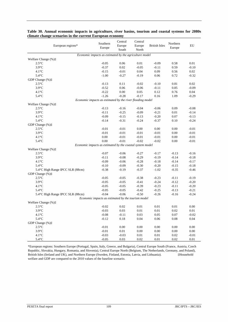
Table 30. Annual economic impacts in agriculture, river basins, tourism and coastal systems for 2080s climate change scenarios in the current European economy
European regions* Southern Europe
Central Europe South
Central Europe North
British Isles Northern Europe EU
Welfare Change (%)‡2.5°C -0.05 0.06 0.01 -0.09 0.58 0.013.9°C -0.37 0.02 -0.05 -0.11 0.59 -0.104.1°C -0.15 -0.01 0.04 0.09 0.56 0.025.4°C -1.00 -0.27 -0.19 0.06 0.72 -0.32
GDP Change (%)‡2.5°C -0.13 0.11 -0.02 -0.10 0.81 0.023.9°C -0.52 0.06 -0.06 -0.11 0.85 -0.094.1°C -0.22 0.00 0.05 0.12 0.76 0.045.4°C -1.26 -0.28 -0.17 0.16 1.09 -0.29
Welfare Change (%)‡2.5°C -0.13 -0.16 -0.04 -0.06 0.09 -0.083.9°C -0.11 -0.25 -0.09 -0.21 0.01 -0.144.1°C -0.09 -0.15 -0.13 -0.20 0.07 -0.135.4°C -0.14 -0.31 -0.24 -0.37 0.10 -0.24
GDP Change (%)‡2.5°C -0.01 -0.01 0.00 0.00 0.00 -0.013.9°C -0.01 -0.01 -0.01 -0.01 0.00 -0.014.1°C 0.00 -0.01 -0.01 -0.01 0.00 -0.015.4°C 0.00 -0.01 -0.02 -0.02 0.00 -0.01
Welfare Change (%)‡2.5°C -0.07 -0.06 -0.27 -0.17 -0.13 -0.163.9°C -0.11 -0.08 -0.29 -0.19 -0.14 -0.184.1°C -0.09 -0.06 -0.28 -0.18 -0.14 -0.175.4°C -0.10 -0.09 -0.30 -0.20 -0.15 -0.185.4°C High Range IPCC SLR (88cm) -0.38 -0.19 -0.37 -1.02 -0.35 -0.46
GDP Change (%)‡2.5°C -0.05 -0.05 -0.38 -0.23 -0.11 -0.193.9°C -0.05 -0.05 -0.41 -0.24 -0.12 -0.204.1°C -0.05 -0.05 -0.39 -0.23 -0.11 -0.205.4°C -0.05 -0.05 -0.42 -0.25 -0.13 -0.215.4°C High Range IPCC SLR (88cm) -0.04 -0.06 -0.50 -0.26 -0.16 -0.24
Welfare Change (%)‡2.5°C -0.02 0.02 0.01 0.01 0.01 0.003.9°C -0.03 0.03 0.01 0.01 0.02 0.014.1°C -0.08 -0.11 0.03 0.05 0.07 -0.025.4°C -0.12 0.18 0.04 0.06 0.08 0.04
GDP Change (%)‡2.5°C -0.01 0.00 0.00 0.00 0.00 0.003.9°C -0.01 0.01 0.00 0.00 0.00 0.004.1°C -0.03 -0.03 0.01 0.01 0.02 -0.015.4°C -0.05 0.03 0.02 0.01 0.02 0.01
Economic impacts as estimated by the river flooding model
Economic impacts as estimated by the agriculture model
*European regions: Southern Europe (Portugal, Spain, Italy, Greece, and Bulgaria), Central Europe South (France, Austria, Czech Republic, Slovakia, Hungary, Romania, and Slovenia), Central Europe North (Belgium, The Netherlands, Germany, and Poland), British Isles (Ireland and UK), and Northern Europe (Sweden, Finland, Estonia, Latvia, and Lithuania). ‡Household welfare and GDP are compared to the 2010 values of the baseline scenario.
Economic impacts as estimated by the coastal system model
Economic impacts as estimated by the tourism model
PESETA final report 109 JRC/IPTS – JRC/IES

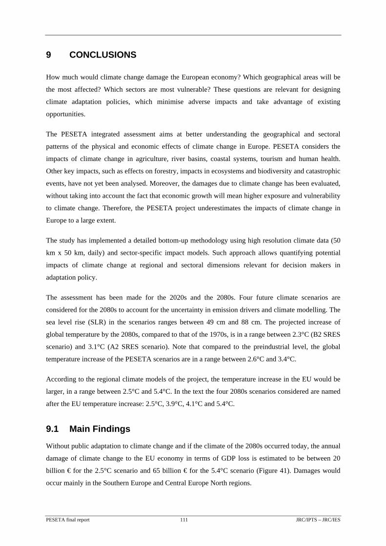
9 CONCLUSIONS
How much would climate change damage the European economy? Which geographical areas will be
the most affected? Which sectors are most vulnerable? These questions are relevant for designing
climate adaptation policies, which minimise adverse impacts and take advantage of existing
opportunities.
The PESETA integrated assessment aims at better understanding the geographical and sectoral
patterns of the physical and economic effects of climate change in Europe. PESETA considers the
impacts of climate change in agriculture, river basins, coastal systems, tourism and human health.
Other key impacts, such as effects on forestry, impacts in ecosystems and biodiversity and catastrophic
events, have not yet been analysed. Moreover, the damages due to climate change has been evaluated,
without taking into account the fact that economic growth will mean higher exposure and vulnerability
to climate change. Therefore, the PESETA project underestimates the impacts of climate change in
Europe to a large extent.
The study has implemented a detailed bottom-up methodology using high resolution climate data (50
km x 50 km, daily) and sector-specific impact models. Such approach allows quantifying potential
impacts of climate change at regional and sectoral dimensions relevant for decision makers in
adaptation policy.
The assessment has been made for the 2020s and the 2080s. Four future climate scenarios are
considered for the 2080s to account for the uncertainty in emission drivers and climate modelling. The
sea level rise (SLR) in the scenarios ranges between 49 cm and 88 cm. The projected increase of
global temperature by the 2080s, compared to that of the 1970s, is in a range between 2.3°C (B2 SRES
scenario) and 3.1°C (A2 SRES scenario). Note that compared to the preindustrial level, the global
temperature increase of the PESETA scenarios are in a range between 2.6°C and 3.4°C.
According to the regional climate models of the project, the temperature increase in the EU would be
larger, in a range between 2.5°C and 5.4°C. In the text the four 2080s scenarios considered are named
after the EU temperature increase: 2.5°C, 3.9°C, 4.1°C and 5.4°C.
9.1 Main Findings
Without public adaptation to climate change and if the climate of the 2080s occurred today, the annual
damage of climate change to the EU economy in terms of GDP loss is estimated to be between 20
billion € for the 2.5°C scenario and 65 billion € for the 5.4°C scenario (Figure 41). Damages would
occur mainly in the Southern Europe and Central Europe North regions.
PESETA final report 111 JRC/IPTS – JRC/IES
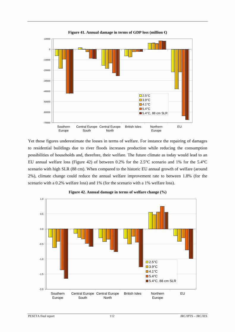
Figure 41. Annual damage in terms of GDP loss (million €)
-70000
-60000
-50000
-40000
-30000
-20000
-10000
0
10000
SouthernEurope
Central EuropeSouth
Central EuropeNorth
British Isles NorthernEurope
EU
2.5°C3.9°C4.1°C5.4°C5.4°C, 88 cm SLR
Yet those figures underestimate the losses in terms of welfare. For instance the repairing of damages to residential buildings due to river floods increases production while reducing the consumption possibilities of households and, therefore, their welfare. The future climate as today would lead to an EU annual welfare loss (Figure 42) of between 0.2% for the 2.5°C scenario and 1% for the 5.4°C scenario with high SLR (88 cm). When compared to the historic EU annual growth of welfare (around 2%), climate change could reduce the annual welfare improvement rate to between 1.8% (for the scenario with a 0.2% welfare loss) and 1% (for the scenario with a 1% welfare loss).
Figure 42. Annual damage in terms of welfare change (%)
-2.0
-1.5
-1.0
-0.5
0.0
0.5
1.0
SouthernEurope
Central EuropeSouth
Central EuropeNorth
British Isles NorthernEurope
EU
2.5°C3.9°C4.1°C5.4°C5.4°C, 88 cm SLR
PESETA final report 112 JRC/IPTS – JRC/IES
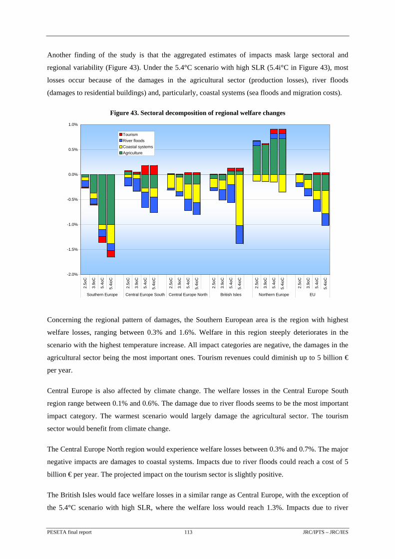
Another finding of the study is that the aggregated estimates of impacts mask large sectoral and
regional variability (Figure 43). Under the 5.4°C scenario with high SLR (5.4i°C in Figure 43), most
losses occur because of the damages in the agricultural sector (production losses), river floods
(damages to residential buildings) and, particularly, coastal systems (sea floods and migration costs).
Figure 43. Sectoral decomposition of regional welfare changes
-2.0%
-1.5%
-1.0%
-0.5%
0.0%
0.5%
1.0%
2.5o
C
3.9o
C
5.4o
C
5.4i
oC
2.5o
C
3.9o
C
5.4o
C
5.4i
oC
2.5o
C
3.9o
C
5.4o
C
5.4i
oC
2.5o
C
3.9o
C
5.4o
C
5.4i
oC
2.5o
C
3.9o
C
5.4o
C
5.4i
oC
2.5o
C
3.9o
C
5.4o
C
5.4i
oC
Southern Europe Central Europe South Central Europe North British Isles Northern Europe EU
TourismRiver floodsCoastal systemsAgriculture
Concerning the regional pattern of damages, the Southern European area is the region with highest
welfare losses, ranging between 0.3% and 1.6%. Welfare in this region steeply deteriorates in the
scenario with the highest temperature increase. All impact categories are negative, the damages in the
agricultural sector being the most important ones. Tourism revenues could diminish up to 5 billion €
per year.
Central Europe is also affected by climate change. The welfare losses in the Central Europe South
region range between 0.1% and 0.6%. The damage due to river floods seems to be the most important
impact category. The warmest scenario would largely damage the agricultural sector. The tourism
sector would benefit from climate change.
The Central Europe North region would experience welfare losses between 0.3% and 0.7%. The major
negative impacts are damages to coastal systems. Impacts due to river floods could reach a cost of 5
billion € per year. The projected impact on the tourism sector is slightly positive.
The British Isles would face welfare losses in a similar range as Central Europe, with the exception of
the 5.4°C scenario with high SLR, where the welfare loss would reach 1.3%. Impacts due to river
PESETA final report 113 JRC/IPTS – JRC/IES
floods are quite negative in all scenarios, as well as impacts to coastal systems, particularly under an
SLR of 88 cm. The impacts on the tourism sector are positive, with up to 4.5 billion € in additional
tourist revenues.
Northern Europe is the only EU area with welfare gains in all scenarios, ranging between 0.5% and
0.7%, mainly thanks to the large positive impacts in the agricultural sector, fewer river floods damages
and higher tourism revenues. However, damages in coastal systems could be significant.
Public adaptation measures have only been modelled in the coastal areas assessment, due to data gaps
and methodological limitations in the rest of sectors. The PESETA study shows that adaptation can
largely reduce the impacts in coastal systems. Earlier assessments also indicate that adaptation policies
could be particularly cost-efficient there (Tol et al., 2008).
Additionally, PESETA analyses the impacts of climate change on human health in the 2080s without
acclimatisation. The estimated range of increase in annual heat-related mortalities is between 60,000
and 165,000, while the range of diminution of cold-related mortalities is between 60,000 and 250,000.
Acclimatisation to warmer climate in summer would reduce the projected mortality changes by a
factor of five. Heatwaves have not been considered in the project.
The aggregated damages of PESETA can be compared to other studies. The PESETA estimates are
lower because the coverage of impacts with market effects is narrower in the PESETA project and the
non market components of the damages are not taken into account either. Thus, for instance,
Fankhauser and Tol (1996) estimate the overall GDP loss for the EU at 1.4%, under a scenario
doubling the CO2–equivalent concentration (to 550 ppmv), compared to preindustrial levels. The
PESETA 5.4°C scenario with high SLR, which would lead to a concentration level of 710 ppmv, has
an estimated annual GDP and welfare loss of 0.5% and 1%, respectively.
9.2 Caveats and Uncertainties
When interpreting the results from the PESETA project, it is essential to take into account the many
caveats of the research project, mainly arisen from the many uncertainties affecting all stages of the
integrated assessment.
Uncertainties are inherent to climate impact assessment as they are present in all stages of the
integrated assessment (IPCC, 2004) and, in particular, are associated with each of the specific models
used: climate models, sectoral physical impact models and economic valuation models. Uncertainty
appears in the input side of the model (value uncertainty) and in the structural specification of the
model (structural uncertainty).
There are four main sources of uncertainty in the overall assessment, associated with:
PESETA final report 114 JRC/IPTS – JRC/IES
- The socioeconomic scenarios driving global GHG emissions.
- The sensitivity of the climate model to GHG concentration.
- The assessment of the physical impact for a given climate scenario.
- The economic valuation of the physical impacts.
Four climate scenarios for the 2080s have been considered in order to address the two first items
(Section 2). The climate scenarios can affect very significantly the results.
Concerning the third source of uncertainty (related to the physical impact models), each sectoral
physical model has its own set of uncertain parameters, and some cases have been explored.
Regarding the economic valuation, in order to avoid making assumptions about the (uncertain)
characteristics of the economy in the 2080s, the overall impact is measured against the current
economic structure. This approach is justified because PESETA does not aim at making projections or
forecasts, but rather at putting in relative terms the sectoral and spatial pattern of impacts in the EU
under different climate scenarios.
As already noted, the PESETA study assessment cannot capture the complete range of the many
possible impacts of climate change on the European economy. Not all impacts that are valued by
markets have been considered (e.g. transport, energy, forestry). The explicit consideration of the effect
due to climate extremes has only been made in the analysis of river floods, and partly in coastal
systems (sea floods). Non-market impact categories have been studied to a very limited extent (human
health effects related to changes in average temperatures). Most of the non market components in the
welfare losses for the impact categories considered are not included either. Other key impacts, e.g. on
biodiversity loss, have not been taken into account. Major economic damages because of catastrophic
events have not been considered either.
Furthermore, from a methodological point of view, while the five impact models have employed the
same climate data, possible inter-sectoral effects could be further explored, such as the consistency of
the tourism, agriculture and river floods sectors concerning water supply and demand.
Another limitation of the study is that the effects of climate change in the rest of the world and their
impact for the EU have not been taken into account. For instance, migration issues or potential rising
agriculture costs globally could have costs or benefits in the EU. Land use-specific policies have not
been considered either.
PESETA final report 115 JRC/IPTS – JRC/IES
PESETA final report 116 JRC/IPTS – JRC/IES
9.3 Further research
What follows is a tentative list of possible relevant issues which could orientate future research,
without intending to be exhaustive (Carter et al., 2007). As the Commission White Paper on
adaptation remarks (European Commission, 2009a), there will be a growing need of high resolution in
climate change impact, adaptation and vulnerability (CCIAV) assessments, mainly for the design and
implementation of adaptation policies. This general need has the following dimensions:
- Space: the regional and local (municipality) scales.
- Time horizon: includes particularly the next few decades, in addition to the usual time window of the
end of the XXI century.
- Sectors and effects: further develop and improve modelling systems able to quantify the
consequences of climate change both on market and non-market sectors, also considering the effects
due to changes in climate variability and extremes, in addition to the usual analysis of the climate
variable mean-related effects. In particular, there seems to be a need to develop methods to quantify
the effects of catastrophic events.
- The cost-benefit analysis of adaptation strategies is not readily available on a European scale and it is
a research area that deserves further efforts.
Moreover, equity issues could be considered more explicitly, going beyond the standard efficiency
analysis. Gainers and losers e.g. per social or income group could be identified for the space and time
resolution of the adaptation assessments.
Concerning the methodological framework, firstly, the cascade of uncertainties in CCIAV assessments
could be dealt with in a more systematic way, i.e. with a probabilistic approach. Secondly, the
consistency of the CCIAV assessments could be improved e.g. by introducing dynamic land-use
scenarios and cross-sectoral consistency issues.
10 REFERENCES
Ackerman, F., Stanton, E.A., Hope, C., Alberth, S. (2009), "Did the Stern review underestimate US and global climate damages?", Energy Policy 37, 2717-2721.
Alcamo, J., Moreno, J.M., Nováky, B., Bindi, M., Corobov, R., Devoy, R.J.N., Giannakopoulos, C., Martin, E., Olesen, J.E., Shvidenko A. (2007), "Europe", in: M.L. Parry, O.F. Canziani, J.P. Palutikof, P.J. van der Linden & C.E. Hanson, (Eds.), Climate Change 2007: Impacts, Adaptation and Vulnerability. Contribution of Working Group II to the Fourth Assessment Report of the Intergovernmental Panel on Climate Change, Cambridge University Press, Cambridge, UK, 541-580.
Amelung, B., Nicholls, S., Viner, D. (2007), "Implications of global climate change for tourism flows and seasonality". Journal of Travel Research, 45, 285-296.
Amelung, B., Viner, D. (2006), "The sustainability of tourism in the Mediterranean: Exploring the future with the tourism climatic index". Journal of Sustainable Tourism, 14, 349-366.
Amelung, B., Moreno A. (2009), "Impacts of climate change in tourism in Europe. PESETA - tourism study", JRC Scientific and Technical Reports, (Forthcoming).
Arnell, N. W., Livermore, M. J. L., Kovats, S., Levy, P. E., Nicholls, R., Parry, M. L., Gaffin, S. R. (2004), "Climate and socio-economic scenarios for global-scale climate change impacts assessments: Characterising the SRES storylines", Global Environmental Change, 14:3-20
Baccini, M., Biggeri, A., Accetta, G., Kosatsky, T., Katsouyanni, K., Analitis, A., Ross Anderson, H., Bisanti, L., D'Ippoliti, D., Danova, J., Forsberg, B., Medina, S., Paldy, A., Rabczenko, D., Schindler, C., Michelozzi, P. (2008), "Effects of apparent temperature on summer mortality in 15 European cities: results of the PHEWE project", Epidemiology, 19.
Bosello, F., Roson, R., Tol, R.S.J. (2007), "Economy-wide estimates of the implications of climate change: Sea level rise", Environmental & Resource Economics 37, 549-571.
Carter, T.R. (2007), "Assessing the adaptive capacity of the Finnish environment and society under a changing climate: FINADAPT", Finnish Environment, 1/2007, 76.
Carter, T.R., Jones, R.N., Lu X., Bhadwal, S., Conde, C., Mearns, L.O., O’Neill, B.C., Rounsevell, M.D.A., Zurek, M.B. (2007), "New assessment methods and the characterisation of future conditions", in: M.L. Parry, O.F., Canziani, J.P., Palutikof, P.J., van der Linden, Hanson, C.E. (Eds.), Climate Change 2007: Impacts, Adaptation and Vulnerability. Contribution of Working Group II to the Fourth Assessment Report of the Intergovernmental Panel on Climate Change, Cambridge University Press, Cambridge, UK, 133-171.
Christensen, J.H., Carter, T., Rummukainen, M. (2007), "Evaluating the performance and utility of regional climate models: the PRUDENCE project", Climatic Change, 81, 1-6.
Christensen, J.H., Christensen, O.B. (2003), "Climate modelling: Severe summertime flooding in Europe", Nature, 421, 805-806.
Ciscar, J.C., Paroussos, L., van Regemorter, D. (2009), "Evaluation of post Kyoto GHG reduction paths", European Review of Energy Markets 7, 1.
Costello, A., Abbas, M., Allen, A., Ball, S., Bell, S., Bellamy, R., Friel, S., Groce, N., Johnson, A., Kett, M., Lee, M., Levy, C., Maslin, M., McCoy, D., McGuire, B., Montgomery, H., Napier, D.,
PESETA final report 117 JRC/IPTS – JRC/IES
Pagel, C., Patel, J., Puppim de Oliveira J.A., et al. (2009), "Managing the health effects of climate change", The Lancet, 373, Issue 9676, 1693 – 1733.
Council of the European Union (2004), Presidency Conclusions – Brussels, 25/26 March 2004, http://europa.eu/european-council/index_en.htm
Council of the European Union (2005), Presidency Conclusions – Brussels, 22/23 March 2005, http://europa.eu/european-council/index_en.htm
Council of the European Union (2007), Presidency Conclusions – Brussels, 8/9 March 2007, http://europa.eu/european-council/index_en.htm
Church, J.A., Gregory, J.M., Huybrechts, P., Kuhn, M., Lambeck, K., Nhuan, M.T., Qin, D., Woodworth, P.L. (2001), "Changes in sea level", in: Houghton, J.T., Ding, Y., Griggs, D.J., Noguer, M., van der Linden, P.J., Xiaosu, D. (Eds.), Climate Change 2001. The Scientific Basis, Cambridge, U.K., Cambridge University Press, 639-693.
Dankers, R., Feyen, L. (2008), "Climate change impact on flood hazard in Europe: An assessment based on high-resolution climate simulations". Journal Geophysical Research – Atmospheres, 113, D19105, doi:10.1029/2007JD009719.
Darwin, R.F., Tol, R.S.J. (2001), "Estimates of the economic effects of sea level rise", Environmental and Resource Economics, 19, 446-129.
Dessai, S. (2003), "Heat stress and mortality in Lisbon Part II. An assessment of the potential impacts of climate change", International Journal of Biometeorology, 48, 37-44.
EEA (2000), "The European Topic Centre on Terrestrial Environment: CORINE land cover raster database 2000 - 100m". European Environment Agency (EEA). Copenhagen, Denmark.
EEA (2004), "Mapping the impacts of recent natural disasters and technological accidents in Europe", Environmental Issue Report No. 35, European Environment Agency (EEA), Copenhagen, Denmark.
EEA (2008), "Impacts of Europe's changing climate – 2008 indicator-based assessment", Joint EEA-JRC-WHO report, EEA Report No 4/2008, JRC Reference Report No JRC47756, European Environment Agency.
European Commission (2007a), "Limiting global climate change to 2 degrees Celsius. The way ahead for 2020 and beyond", COM(2007) 2 final.
European Commission (2007b), Green Paper "Adapting to climate change in Europe – options for EU action ", COM/2007/0354 final.
European Commission (2009a), White Paper "Adapting to climate change: Towards a European framework for action", COM(2009) 147 final.
European Commission (2009b), "Towards a comprehensive climate change agreement in Copenhagen" (European Commission, COM(2009) 39 final.
Fankhauser, S. (1994), “The social costs of greenhouse gas emissions: An expected value approach”. Energy Journal, 15, 157–84.
Fankhauser, S. (1995), Valuing Climate Change—The Economics of the Greenhouse, London: EarthScan.
PESETA final report 118 JRC/IPTS – JRC/IES
Fankhauser, S., Tol, R.S.J. (1996), "Climate change costs. Recent advancements in the economic assessment", Energy Policy, 24, 665-673.
Feyen L., Dankers R., Barredo J.I., Kalas M., Bódis K., de Roo A., Lavalle C. (2006), "PESETA- Flood risk in Europe in a changing climate". Institute of Environment and Sustainability, Joint Research Center, EUR 22313 EN.
Frei, C., Schöll, R., Fukutome, S., Schmidli, J., Vidale, P.L. (2006), "Future change of precipitation extremes in Europe: Intercomparison of scenarios from regional climate models", Journal Geophysical Research-Atmospheres, 111, D06105, doi:10.1029/2005JD005965.
Gallego, J., Peedell, S. (2001), "Using Corine land cover to map population density. Towards agri-environmental indicators", Topic Report 6/2001 European Environment Agency, Copenhagen.
Gordon, C., Cooper, C., Senior, C.A., Banks, H., Gregory, J.M., Johns, T.C., Mitchell, J.F.B., Wood, R.A. (2000), "The simulation of SST, sea ice extents and ocean heat transports in a version of the Hadley Centre coupled model without flux adjustments", Climate Dynamics, 16, 147-168.
Gupta, J., Olzthoorn, X., Rotemberg, E. (2003), "The role of scientific uncertainty in compliance with the Kyoto protocol to the climate change convention", Environmental Science and Policy, 6, 475-486.
G8 (2009). L'Aquila Summit Leaders Declaration; http://www.g8italia2009.it/static/G8_Allegato/G8_Declaration_08_07_09_final,0.pdf
Halsnæs, K., Kühl, J., Olesen, J.E. (2007), "Turning climate change information into economic and health impacts", Climatic Change, 81, 145-162.
Hayhoe, K., Cayan, D., Field, C.B., Peter, Frumhoff, C., Maurer, E.P., Miller, N.L., Moser, S.C., Schneider, S.H., Cahill, K.N., Cleland, E.E., Dale, L., Drapek, R., Hanemann, R.M., Kalkstein, L.S., Lenihan, J., Lunch, C.K., Neilson, R.P., Sheridan, S.C., Verville, J.H. (2004), "Emissions pathways, climate change, and impacts on California", Proceedings of the National Academy of Sciences, 101, 12422-12427.
Hertel, T.W. (1997), Global Trade Analysis: Modelling and Applications, Cambridge University Press.
Hinkel, J., Klein, R.J.T. (2006), "Integrating Knowledge for Assessing Coastal Vulnerability to Climate Change", in: McFadden, L., Penning-Rowsell, E.C. (Eds.), Managing Coastal Vulnerability: An Integrated Approach, Elsevier Science.
Hitz, S., Smith, J. (2004), "Estimating global impacts from climate change", Global Environmental Change, 14, 201-218.
Huizinga, H.J. (2007), "Flood damage functions for EU member states". Technical Report, HKV Consultants. Implemented in the framework of the contract #382441-F1SC awarded by the European Commission - Joint Research Centre.
Iglesias, A., Moneo, M., Garrote, L., Flores, F. (2006), "Drought and water scarcity: current and future vulnerability and risk", in: Garrido, A., Llamas, M.R. (Eds.), Issues in Water Resource Policy, Resources for the Future, Washington DC.
Iglesias, A., Garrote, L., Flores, F., Moneo, M. (2007), "Challenges to manage the risk of water scarcity and climate change in the Mediterranean", Water Resources Management, 21(5), 227-288
PESETA final report 119 JRC/IPTS – JRC/IES
Iglesias, A,, Cancelliere, A,, Cubillo, F., Garrote, L., Wilhite, D.A. (2009a), Coping with drought risk in agriculture and water supply systems: Drought management and policy development in the Mediterranean, Springer, The Netherlands.
Iglesias, A., Garrote, L., Quiroga, S., Moneo M. (2009b), "Impacts of climate change in agriculture in Europe. PESETA-Agriculture study", JRC Scientific and Technical Reports, (Forthcoming).
IPCC (2001), Climate Change 2001. The Scientific Basis, Houghton, J.T., et al. (Eds.), Cambridge Univ. Press, Cambridge, chap. 11.
IPCC (2004), “IPCC Workshop on Describing Scientific Uncertainties in Climate Change to Support Analysis of Risk and of Options”, Workshop Report, Manning, M., et al. (Eds.), http://ipcc-wg1.ucar.edu/meeting/URW/product/URW_Report_v2.pdf
IPCC (2007a), Climate Change 2007: The Physical Science Basis. Contribution of Working Group 1 to the Fourth Assessment Report of the Intergovernmental Panel on Climate Change. Solomon, S., et al. (Eds.), Cambridge Univ. Press, Cambridge, chap. 10.
IPCC (2007b), Appendix I, Climate Change 2007: Impacts, Adaptation and Vulnerability, Contribution of Working Group II to the Fourth Assessment Report of the Intergovernmental Panel on Climate Change, Parry M.L., et al. (Eds.), Cambridge University Press, Cambridge, UK.
Jorgenson, D.W., Goettle, R.J., Hurd, B.H., Smith, J.S. (2004), "U.S. market consequences of climate change", Pew Center on Global Climate Change.
Kovats, S., Lachowyz, K., Armstrong, B., Hunt, A., Markandya, A. (2006), in Metroeconomica et al., Climate Change Impacts and Adaptation: Cross-Regional Research Programme Project E. Study for Department for Environment, Food and Rural Affairs, UK. Available from http://www.defra.gov.uk
Levina, E., Tirpak, D. (2006), "Adaptation to Climate Change: Key Terms", (CON/ENV/EPOC/IEA/SLT(2006)1), OECD.
Mairie de Paris (2007), "Paris Climate Plan: What weather for tomorrow?", Annex to Decision No.
DEVE 2007 – 116 available at
http://www.paris.fr/portail/viewmultimediadocument?multimediadocument-id=66816
Markandya, A., Hunt, A., Ortiz, R., Alberini, A. (2004), “EC NewExt Research Project: Mortality Risk Valuation”, Final Report, Brussels: European Commission.
Mastrandrea, M.D., Schneider, S. (2004), "Probabilistic integrated assessment of "dangerous" climate change", Science, 304, 571.
Mather, S., Viner, D., Graham, T. (2005), "Climate and policy changes: their implications for international tourism flows", in: Hall, C. M., Higham, J. (Eds.), Tourism, Recreation and Climate Change, Channel View Publications, Bristol.
McFadden, L., Nicholls, R.J., Vafeidis, A., Tol, R.S.J. (2007), "A Methodology for Modeling Coastal Space for Global Assessment", Journal of Coastal Research, 23, 911.
McGranahan, G., Balk, D., Anderson, B. (2007), "The rising tide: assessing the risks of climate change and human settlements in low elevation coastal zones", Environment and Urbanization, 19, 17-37.
PESETA final report 120 JRC/IPTS – JRC/IES
McMichael, A.J., Campbell-Lendrum, D., Kovats, R., et al. (2004), "Climate change", in: Ezzati, M., Lopez, A.D., Rodgers, A., & Murray, C.J. (Eds.) Comparative quantification of health risks: global and regional burden of disease due to selected major risk factors, vol. 2. World Health Organisation, Geneva, 1543–1649.
Mearns, L.O., Giorgi, F., Whetton, P., Pabon, D., Hulme, M., Lal, M. (2003), "Guidelines for Use of Climate Scenarios Developed from Regional Climate Model Experiments", Intergovernmental Panel on Climate Change (IPCC) Task Group on Data and Scenario Support for Impacts and Climate Analysis (TGICA), available from: http://www.ipcc-data.org/guidelines/dgm_no1_v1_10-2003.pdf .
Mendelsohn, R., Neumann, J.E. (1999). The Impact of Climate Change on the United States Economy, Cambridge Univ. Press.
Menne, B., Ebi, K.L. (Eds.), (2006), Climate change and adaptation strategies for human health. WHO (Europe).
Metzger, M.J., Rounsevell, M.D.A., Acosta-Michlik, L., Leemans, R., Schröter, D. (2006), "The vulnerability of ecosystem services to land use change", Agriculture, Ecosystems & Environment, 114, 69-85.
Mieczkoswki, Z. (1985), "The Tourism Climatic Index: A method of evaluating world climates for tourism”, Canadian Geographer, 29, 220-233.
Nakicenovic, N., Swart, R. (Eds.), (2000), Intergovernmental Panel on Climate Change. Special Report on Emissions Scenarios, Cambridge Univ. Press, Cambridge.
Nicholls, R.J., Klein, R.J.T. (2005), "Climate change and coastal management on Europe’s coast", in: Vermaat, J.E., Ledoux, L., Turner, K., Salomons, W. (Eds.), Managing European coasts: past, present and future, Springer, Environmental Science Monograph Series, Berlin.
Nicholls, R.J., Klein, R.J.T., Tol, R.S.J. (2006), "Managing coastal vulnerability and climate change: a national to global perspective", in: McFadden, L., Penning-Rowsell, E.C. (Eds.), Managing Coastal Vulnerability: An Integrated Approach, Elsevier Science.
Nicholls, R.J., Tol, R.S.J., Hall, J.W. (2007), "Assessing impacts and responses to global-mean sea-level rise", in: Schlesinger, M. (Ed.), Human-Induced Climate Change: An Interdisciplinary Assessment, Cambridge University Press, Cambridge, U.K.
Nicholls, R.J., Wong, P.P., Burkett, V.R., Codignotto, J.O., Hay, J.E., McLean, R.F., Ragoonaden, S., Woodroffe, C.D. (2007b), "Coastal systems and low-lying areas", in: Parry, M.L., Canziani, O.F., Palutikof, J.P., van der Linden P.J., Hanson, C.E. (Eds.), Climate Change 2007: Impacts, Adaptation and Vulnerability, Contribution of Working Group II to the Fourth Assessment Report of the Intergovernmental Panel on Climate Change, Cambridge University Press, Cambridge, UK, 315-356.
Nordhaus, W. (1992), "An optimal transition path for controlling greenhouse gases", Science, 258, 1315-1319.
Nordhaus, W. (1994), Managing the Global Commons: The Economics of Climate Change, MIT Press, Cambridge, MA.
Nordhaus, W., Yang, Z. (1996), "A regional dynamic general-equilibrium model of alternative climate-change strategies", American Economic Review, 86, 741-765.
Nordhaus, W. (2007), "Critical Assumptions in the Stern Review on Climate Change", Science, 317, 201-202.
PESETA final report 121 JRC/IPTS – JRC/IES
Olensen, J.O., Bindi, M. (2002), "Consequences of climate change for European agricultural productivity, land use and policy", European Journal of Agronomy, 16, 239–262.
Parry, M. (Ed.), (2000), Assessment of Potential Effects and Adaptations for Climate Change in Europe (ACACIA), University of East Anglia, Norwich, UK.
Parry, M.L., Rosenzweig, C., Iglesias, A., Livermore, M., Fischer, G. (2004), "Effects of climate change on global food production under SRES emissions and socio-economic scenarios", Global Environmental Change, 14, 53-67.
Rahmstorf, S., Cazenave, A., Church, J.A., Hansen, J.E., Keeling, R.F., Parker, D.E., Somerville R.C.J. (2007), "Recent climate observations compared to projections", Science, 316, 709.
Richards, J., Nicholls R.J. (2009), "Impacts of climate change in coastal systems in Europe. PESETA-Coastal Systems study", JRC Scientific and Technical Reports, (Forthcoming).
Roeckner, E., Oberhuber, J.M., Bacher, A., Christoph, M., Kirchner, I. (1996), "ENSO variability and atmospheric response in a global coupled atmosphere-ocean GCM", Climate Dynamics, 12, 737-754.
Rosenzweig, C., Iglesias, A. (2008), "The use of crop models for international climate change impact assessment", in: Tsuji, G. Y., Hoogenboom, G., Thornton, P.K. (Eds), Understanding Options for Agricultural Production, Kluwer Academic Publishers, Dordrecht, The Netherlands.
Rosenzweig, C., & Iglesias, A. (2002), "Climate changes in the Mediterranean: Physical aspects and effects on agriculture", in: H.J. Bolle, (Ed.), Mediterranean Climate, Springer, New York.
Rosenzweig, C., Iglesias, A. (1994), (Eds.), "Implications of climate change for international agriculture: Crop modeling study", U.S. Environmental Protection Agency, EPA 230-B-94-003, Washington DC.
Roshydromet (2005), "Strategic prediction for the period of up to 2010-2015 of climate change expected in Russia and its impact on sectors of the Russian national economy", Federal Service for Hydrometeorology and Environmental Monitoring (Roshydromet), Moscow. http://www.meteorf.ru/en_default_doc.aspx?RgmFolderID=bd22d532-faa3-4e23-9525-420c9cbff936&RgmDocID=b23063af-5d85-40b2-8c97-7d77b45886ae
Rotmans, J., Dowlatabadi H. (1998), "Integrated assessment modelling", in: Rayner, S., Malone, E. (Eds.), Human Choice and Climate Change-Tools for Policy Analysis, Battelle Press, Columbus, OH., 291-377.
Rotmans, J., Hulme, M. & Downing, T.E. (1994), "Climate change implications for Europe: an application of the ESCAPE model", Global Enviromental Change, 4, 97-124.
Russ, P., Ciscar J.C, Saveyn, B., Soria, A., Szabó, L., van Ierland, T., van Regemorter, D., Virdis, R. (2009), " Economic assessment of post-2012 global climate policies - Analysis of greenhouse gas emission reduction scenarios with the POLES and GEM-E3 models", JRC Scientific and Technical Reports, EUR 23768 EN.
Ruth, M., Donaghy, K., Kishen, P. (2006), Regional Climate Change and Variability. Impacts and Responses. Edward Elgar.
Schröter, D., et al. (2005), "Ecosystem service supply and vulnerability to global change in Europe", Science, 310, 1333-1337.
Scott, D., et al. (2008), "Climate change and tourism – Responding to global challenges", United Nations World Tourism Organization, Madrid.
Stern, N. (2007), The Stern Review of the Economics of Climate Change, Cambridge University Press.
PESETA final report 122 JRC/IPTS – JRC/IES
PESETA final report 123 JRC/IPTS – JRC/IES
Stern, N., Taylor, C. (2007), "Climate change: Risk, ethics, and the Stern review". Science, 317, 203-204.
Shoven, J.B., Whalley, Y.J. (1992), Applying General Equilibrium, Cambridge University Press.
Tol, R.S.J. (2005), "The DIVA model: socio-economic scenarios, impacts and adaptation, and world heritage", http://diva.demis.nl/files/folders/downloads/entry25.aspx
Tol, R.S.J., Klein, R.J.T., Nicholls R.J. (2008), "Towards successful adaptation to sea-level rise along Europe's coasts", Journal of Coastal Research, 24, 432-450.
Tol, R.S.J. (2009), "The Economic Effects of Climate Change", Journal of Economic Perspectives, 23, 29-51.
Vafeidis, A.T., et al. (2004), "A global database for coastal vulnerability analysis", Land Ocean Interactions in the Coastal Zone (LOICZ) Newsletter, No. 33.
van der Knijff, J., Younis, J., De Roo, A. (2008), "LISFLOOD: a GIS-based distributed model for river basin scale water balance and flood simulation", International Journal of Geographical Information Science, doi 10.1080/13658810802549154.
van Regemorter, D. (2005), "GEM-E3. Computable General Equilibrium Model for studying Economy-Energy-Environment Interactions for Europe and the World", http://www.gem-e3.net/download/GEMmodel.pdf
Watkiss, P., Horrocks, L., Pye, S., Searl, A., Hunt A. (2009), "Impacts of climate change in human health in Europe. PESETA-Human Health study", JRC Scientific and Technical Reports, (Forthcoming).
Wilby, R.L. (2005), "Uncertainty in water resource model parameters used for climate change impact assessment", Hydrological Processes, 19, 3201–3219.

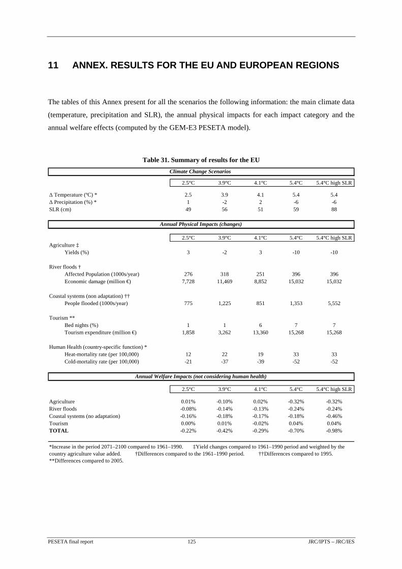
11 ANNEX. RESULTS FOR THE EU AND EUROPEAN REGIONS
The tables of this Annex present for all the scenarios the following information: the main climate data
(temperature, precipitation and SLR), the annual physical impacts for each impact category and the
annual welfare effects (computed by the GEM-E3 PESETA model).
Table 31. Summary of results for the EU
2.5°C 3.9°C 4.1°C 5.4°C 5.4°C high SLR
Δ Temperature (ºC) * 2.5 3.9 4.1 5.4 5.4Δ Precipitation (%) * 1 -2 2 -6 -6SLR (cm) 49 56 51 59 88
2.5°C 3.9°C 4.1°C 5.4°C 5.4°C high SLRAgriculture ‡
Yields (%) 3 -2 3 -10 -10
River floods †Affected Population (1000s/year) 276 318 251 396 396Economic damage (million €) 7,728 11,469 8,852 15,032 15,032
Coastal systems (non adaptation) ††People flooded (1000s/year) 775 1,225 851 1,353 5,552
Tourism **Bed nights (%) 1 1 6 7 7Tourism expenditure (million €) 1,858 3,262 13,360 15,268 15,268
Human Health (country-specific function) *Heat-mortality rate (per 100,000) 12 22 19 33 33Cold-mortality rate (per 100,000) -21 -37 -39 -52 -52
2.5°C 3.9°C 4.1°C 5.4°C 5.4°C high SLR
Agriculture 0.01% -0.10% 0.02% -0.32% -0.32%River floods -0.08% -0.14% -0.13% -0.24% -0.24%Coastal systems (no adaptation) -0.16% -0.18% -0.17% -0.18% -0.46%Tourism 0.00% 0.01% -0.02% 0.04% 0.04%TOTAL -0.22% -0.42% -0.29% -0.70% -0.98%
*Increase in the period 2071–2100 compared to 1961–1990. ‡Yield changes compared to 1961–1990 period and weighted by the country agriculture value added. †Differences compared to the 1961–1990 period. ††Differences compared to 1995. **Differences compared to 2005.
Climate Change Scenarios
Annual Physical Impacts (changes)
Annual Welfare Impacts (not considering human health)
PESETA final report 125 JRC/IPTS – JRC/IES
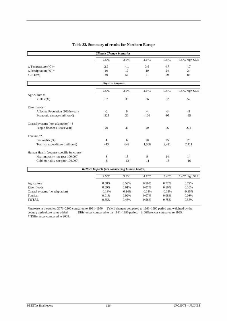
Table 32. Summary of results for Northern Europe
2.5°C 3.9°C 4.1°C 5.4°C 5.4°C high SLR
Δ Temperature (ºC) * 2.9 4.1 3.6 4.7 4.7Δ Precipitation (%) * 10 10 19 24 24SLR (cm) 49 56 51 59 88
2.5°C 3.9°C 4.1°C 5.4°C 5.4°C high SLRAgriculture ‡
Yields (%) 37 39 36 52 52
River floods †Affected Population (1000s/year) -2 9 -4 -3 -3Economic damage (million €) -325 20 -100 -95 -95
Coastal systems (non adaptation) ††People flooded (1000s/year) 20 40 20 56 272
Tourism **Bed nights (%) 4 6 20 25 25Tourism expenditure (million €) 443 642 1,888 2,411 2,411
Human Health (country-specific function) *Heat-mortality rate (per 100,000) 8 15 9 14 14Cold-mortality rate (per 100,000) -8 -13 -11 -16 -16
2.5°C 3.9°C 4.1°C 5.4°C 5.4°C high SLR
Agriculture 0.58% 0.59% 0.56% 0.72% 0.72%River floods 0.09% 0.01% 0.07% 0.10% 0.10%Coastal systems (no adaptation) -0.13% -0.14% -0.14% -0.15% -0.35%Tourism 0.01% 0.02% 0.07% 0.08% 0.08%TOTAL 0.55% 0.48% 0.56% 0.75% 0.55%
*Increase in the period 2071–2100 compared to 1961–1990. ‡Yield changes compared to 1961–1990 period and weighted by the country agriculture value added. †Differences compared to the 1961–1990 period. ††Differences compared to 1995. **Differences compared to 2005.
Climate Change Scenarios
Physical Impacts
Welfare Impacts (not considering human health)
PESETA final report 126 JRC/IPTS – JRC/IES

Table 33. Summary of results for British Isles
2.5°C 3.9°C 4.1°C 5.4°C 5.4°C high SLR
Δ Temperature (ºC) * 1.6 2.5 3.2 3.9 3.9Δ Precipitation (%) * -5 -2 10 5 5SLR (cm) 49 56 51 59 88
2.5°C 3.9°C 4.1°C 5.4°C 5.4°C high SLRAgriculture ‡
Yields (%) -9 -11 15 19 19
River floods †Affected Population (1000s/year) 12 48 43 79 79Economic damage (million €) 755 2,854 2,778 4,966 4,966
Coastal systems (non adaptation) ††People flooded (1000s/year) 70 136 86 207 1279
Tourism **Bed nights (%) 3 4 14 18 18Tourism expenditure (million €) 680 932 3,587 4,546 4,546
Human Health (country-specific function) *Heat-mortality rate (per 100,000) 4 8 7 10 10Cold-mortality rate (per 100,000) -27 -48 -57 -75 -75
2.5°C 3.9°C 4.1°C 5.4°C 5.4°C high SLR
Agriculture -0.09% -0.11% 0.09% 0.06% 0.06%River floods -0.06% -0.21% -0.20% -0.37% -0.37%Coastal systems (no adaptation) -0.17% -0.19% -0.18% -0.20% -1.02%Tourism 0.01% 0.01% 0.05% 0.06% 0.06%TOTAL -0.31% -0.50% -0.24% -0.44% -1.26%
*Increase in the period 2071–2100 compared to 1961–1990. ‡Yield changes compared to 1961–1990 period and weighted by the country agriculture value added. †Differences compared to the 1961–1990 period. ††Differences compared to 1995. **Differences compared to 2005.
Climate Change Scenarios
Physical Impacts
Welfare Impacts (not considering human health)
PESETA final report 127 JRC/IPTS – JRC/IES
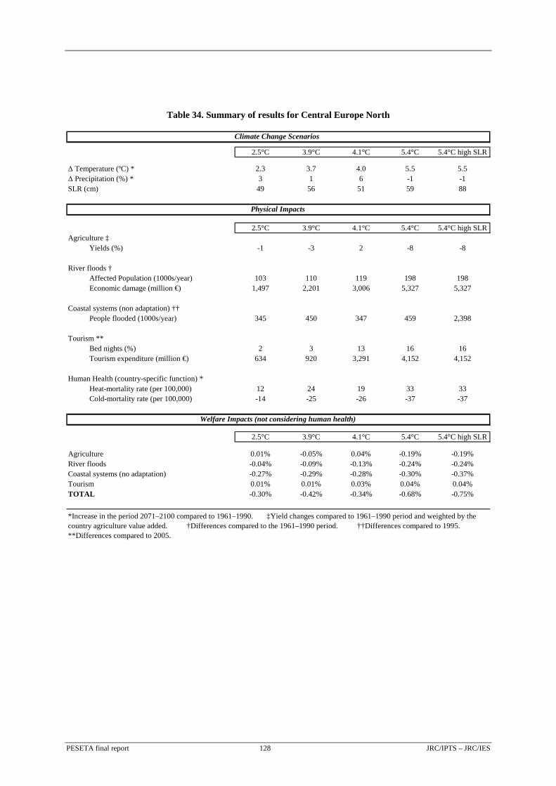
Table 34. Summary of results for Central Europe North
2.5°C 3.9°C 4.1°C 5.4°C 5.4°C high SLR
Δ Temperature (ºC) * 2.3 3.7 4.0 5.5 5.5Δ Precipitation (%) * 3 1 6 -1 -1SLR (cm) 49 56 51 59 88
2.5°C 3.9°C 4.1°C 5.4°C 5.4°C high SLRAgriculture ‡
Yields (%) -1 -3 2 -8 -8
River floods †Affected Population (1000s/year) 103 110 119 198 198Economic damage (million €) 1,497 2,201 3,006 5,327 5,327
Coastal systems (non adaptation) ††People flooded (1000s/year) 345 450 347 459 2,398
Tourism **Bed nights (%) 2 3 13 16 16Tourism expenditure (million €) 634 920 3,291 4,152 4,152
Human Health (country-specific function) *Heat-mortality rate (per 100,000) 12 24 19 33 33Cold-mortality rate (per 100,000) -14 -25 -26 -37 -37
2.5°C 3.9°C 4.1°C 5.4°C 5.4°C high SLR
Agriculture 0.01% -0.05% 0.04% -0.19% -0.19%River floods -0.04% -0.09% -0.13% -0.24% -0.24%Coastal systems (no adaptation) -0.27% -0.29% -0.28% -0.30% -0.37%Tourism 0.01% 0.01% 0.03% 0.04% 0.04%TOTAL -0.30% -0.42% -0.34% -0.68% -0.75%
*Increase in the period 2071–2100 compared to 1961–1990. ‡Yield changes compared to 1961–1990 period and weighted by the country agriculture value added. †Differences compared to the 1961–1990 period. ††Differences compared to 1995. **Differences compared to 2005.
Climate Change Scenarios
Physical Impacts
Welfare Impacts (not considering human health)
PESETA final report 128 JRC/IPTS – JRC/IES
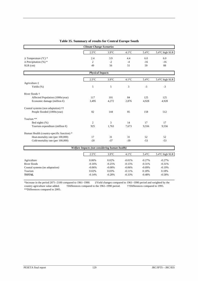
Table 35. Summary of results for Central Europe South
2.5°C 3.9°C 4.1°C 5.4°C 5.4°C high SLR
Δ Temperature (ºC) * 2.4 3.9 4.4 6.0 6.0Δ Precipitation (%) * 2 -2 -4 -16 -16SLR (cm) 49 56 51 59 88
2.5°C 3.9°C 4.1°C 5.4°C 5.4°C high SLRAgriculture ‡
Yields (%) 5 5 3 -3 -3
River floods †Affected Population (1000s/year) 117 101 84 125 125Economic damage (million €) 3,495 4,272 2,876 4,928 4,928
Coastal systems (non adaptation) ††People flooded (1000s/year) 82 144 85 158 512
Tourism **Bed nights (%) 2 3 14 17 17Tourism expenditure (million €) 925 1,763 7,673 9,556 9,556
Human Health (country-specific function) *Heat-mortality rate (per 100,000) 17 31 31 52 52Cold-mortality rate (per 100,000) -20 -37 -39 -53 -53
2.5°C 3.9°C 4.1°C 5.4°C 5.4°C high SLR
Agriculture 0.06% 0.02% -0.01% -0.27% -0.27%River floods -0.16% -0.25% -0.15% -0.31% -0.31%Coastal systems (no adaptation) -0.06% -0.08% -0.06% -0.09% -0.19%Tourism 0.02% 0.03% -0.11% 0.18% 0.18%TOTAL -0.14% -0.28% -0.33% -0.48% -0.58%
*Increase in the period 2071–2100 compared to 1961–1990. ‡Yield changes compared to 1961–1990 period and weighted by the country agriculture value added. †Differences compared to the 1961–1990 period. ††Differences compared to 1995. **Differences compared to 2005.
Climate Change Scenarios
Physical Impacts
Welfare Impacts (not considering human health)
PESETA final report 129 JRC/IPTS – JRC/IES

Table 36. Summary of results for Southern Europe
2.5°C 3.9°C 4.1°C 5.4°C 5.4°C high SLR
Δ Temperature (ºC) * 2.6 4.1 4.3 5.6 5.6Δ Precipitation (%) * -7 -15 -13 -28 -28SLR (cm) 49 56 51 59 88
2.5°C 3.9°C 4.1°C 5.4°C 5.4°C high SLRAgriculture ‡
Yields (%) 0 -12 -4 -27 -27
River floods †Affected Population (1000s/year) 46 49 9 -4 -4Economic damage (million €) 2,306 2,122 291 -95 -95
Coastal systems (non adaptation) ††People flooded (1000s/year) 258 456 313 474 1091
Tourism **Bed nights (%) -1 -1 -2 -4 -4Tourism expenditure (million €) -824 -995 -3,080 -5,398 -5,398
Human Health (country-specific function) *Heat-mortality rate (per 100,000) 11 18 18 28 28Cold-mortality rate (per 100,000) -28 -52 -49 -64 -64
2.5°C 3.9°C 4.1°C 5.4°C 5.4°C high SLR
Agriculture -0.05% -0.37% -0.15% -1.00% -1.00%River floods -0.13% -0.11% -0.09% -0.14% -0.14%Coastal systems (no adaptation) -0.07% -0.11% -0.09% -0.10% -0.38%Tourism -0.02% -0.03% -0.08% -0.12% -0.12%TOTAL -0.27% -0.62% -0.41% -1.36% -1.65%
*Increase in the period 2071–2100 compared to 1961–1990. ‡Yield changes compared to 1961–1990 period and weighted by the country agriculture value added. †Differences compared to the 1961–1990 period. ††Differences compared to 1995. **Differences compared to 2005.
Climate Change Scenarios
Physical Impacts
Welfare Impacts (not considering human health)
PESETA final report 130 JRC/IPTS – JRC/IES
European Commission EUR 24093 EN – Joint Research Centre – Institute for Prospective Technological Studies – Institute for Environment and Sustainability Title: Climate change impacts in Europe. Final report of the PESETA research project Authors: Ciscar, J.C., Iglesias, A., Feyen, L., Goodess, C.M., Szabó, L., Christensen, O.B., Nicholls, R., Amelung, B., Watkiss, P., Bosello, F., Dankers, R., Garrote, L., Hunt, A., Horrocks, L., Moneo, M., Moreno, A., Pye, S., Quiroga, S., van Regemorter, D., Richards, J., Roson, R., Soria, A. Luxembourg: Office for Official Publications of the European Communities 2009 EUR – Scientific and Technical Research series – ISSN 1018-5593 ISBN 978-92-79-14272-7 DOI 10.2791/32500 Abstract The PESETA research project integrates a set of high-resolution climate change projections and physical models into an economic modelling framework to quantify the impacts of climate change on vulnerable aspects of Europe. Four market impact categories are considered (agriculture, river floods, coastal systems, and tourism) and one non-market category (human health). Considering the market impacts, without public adaptation and if the climate of the 2080s occurred today, the EU annual welfare loss would be in the range of 0.2% to 1%, depending on the climate scenario. However, there is large variation across different climate futures, EU regions and impact categories. Scenarios with warmer temperatures and higher sea level rise result in more severe economic damage for the EU. Southern Europe, the British Isles and Central Europe North appear to be the most sensitive regions to climate change. Northern Europe is the only region with net economic benefits, mainly driven by the positive effects in agriculture. Concerning the contribution to the overall effects, coastal systems, agriculture and river flooding are the most important ones.
How to obtain EU publications Our priced publications are available from EU Bookshop (http://bookshop.europa.eu), where you can place an order with the sales agent of your choice. The Publications Office has a worldwide network of sales agents. You can obtain their contact details by sending a fax to (352) 29 29-42758.

The mission of the Joint Research Centre is to provide customer-driven scientific and technical support for the conception, development, implementation and monitoring of European Union policies. As a service of the European Commission, the Joint Research Centre functions as a reference centre of science and technology for the Union. Close to the policy-making process, it serves the common interest of the Member States, while being independent of special interests, whether private or national.
LF-N
A-24093-E
N-C


![Second EC-JRC aromatic compounds intercomparison with automatic analyzer …publications.jrc.ec.europa.eu/repository/bitstream... · 22523 EN], this intercomparison exercise follows](https://img.pdfslide.us/doc/110x75/612a209d98299b656d0b7fd0/second-ec-jrc-aromatic-compounds-intercomparison-with-automatic-analyzer-22523-en.jpg)