Embed Size (px)
Citation preview

Food Research International 55 (2014) 137–149
Contents lists available at ScienceDirect
Food Research International
j ourna l homepage: www.e lsev ie r .com/ locate / foodres
Review
Observations on the use of statistical methods in Food Scienceand Technology
Daniel Granato a,⁎, Verônica Maria de Araújo Calado b, Basil Jarvis c
a State University of Ponta Grossa, Food Science and Technology Graduate Programme, Av. Carlos Cavalcanti, 4748, Uvaranas Campus, 84030-900 Ponta Grossa, Brazilb Federal University of Rio de Janeiro, School of Chemistry, Rio de Janeiro, Brazilc The University of Reading, Department of Food and Nutrition Sciences, School of Chemistry, Food and Pharmacy, Whiteknights, Reading, Berkshire RG6 6AP, United Kingdom
⁎ Corresponding author.E-mail addresses: [email protected] (D. Granato), c
(V.M. de Araújo Calado), [email protected] (B. Ja
0963-9969/$ – see front matter © 2013 Elsevier Ltd. All rihttp://dx.doi.org/10.1016/j.foodres.2013.10.024
a b s t r a c t
a r t i c l e i n f oArticle history:Received 4 August 2013Accepted 17 October 2013
Keywords:CorrelationANOVAStatisticsRegressionNormalityMultiple comparison tests
Statistical methods are important aids to detect trends, explore relationships and draw conclusions from exper-imental data. However, it is not uncommon to find that many researchers apply statistical tests without firstchecking whether they are appropriate for the intended application. The aim of this paper is to present someof themore important univariate and bivariate parametric and non-parametric statistical techniques and to high-light their uses based onpractical examples in Food Science and Technology. The underlying requirements for useof particular statistical tests, together with their advantages and disadvantages in practical applications are alsodiscussed, such as the need to check for normality and homogeneity of variances prior to the comparison oftwo or more sample sets in inference tests, correlation and regression analysis.
© 2013 Elsevier Ltd. All rights reserved.
Contents
1. Introduction . . . . . . . . . . . . . . . . . . . . . . . . . . . . . . . . . . . . . . . . . . . . . . . . . . . . . . . . . . . . . . 1372. Concepts of statistics applied in Food Science . . . . . . . . . . . . . . . . . . . . . . . . . . . . . . . . . . . . . . . . . . . . . . . 138
2.1. Normality and homoscedasticity . . . . . . . . . . . . . . . . . . . . . . . . . . . . . . . . . . . . . . . . . . . . . . . . . 1402.1.1. Normality of data: is it truly important? . . . . . . . . . . . . . . . . . . . . . . . . . . . . . . . . . . . . . . . . . 1402.1.2. Equality of variances: importance and concepts . . . . . . . . . . . . . . . . . . . . . . . . . . . . . . . . . . . . . . 141
2.2. Parametric statistics in Food Science . . . . . . . . . . . . . . . . . . . . . . . . . . . . . . . . . . . . . . . . . . . . . . . 1422.2.1. Comparing two samples/treatments . . . . . . . . . . . . . . . . . . . . . . . . . . . . . . . . . . . . . . . . . . . 1422.2.2. Analysis of variances for three or more data sets . . . . . . . . . . . . . . . . . . . . . . . . . . . . . . . . . . . . . . 1432.2.3. Post-hoc tests to compare three or more samples/treatments . . . . . . . . . . . . . . . . . . . . . . . . . . . . . . . . 143
2.3. Non-parametric statistics in Food Science . . . . . . . . . . . . . . . . . . . . . . . . . . . . . . . . . . . . . . . . . . . . . 1442.3.1. Comparing two samples/treatments . . . . . . . . . . . . . . . . . . . . . . . . . . . . . . . . . . . . . . . . . . . 1442.3.2. Comparing three or more samples or treatments . . . . . . . . . . . . . . . . . . . . . . . . . . . . . . . . . . . . . 144
2.4. Bivariate correlation analysis . . . . . . . . . . . . . . . . . . . . . . . . . . . . . . . . . . . . . . . . . . . . . . . . . . . 1452.5. Regression analysis . . . . . . . . . . . . . . . . . . . . . . . . . . . . . . . . . . . . . . . . . . . . . . . . . . . . . . . 1472.6. Other statistical techniques . . . . . . . . . . . . . . . . . . . . . . . . . . . . . . . . . . . . . . . . . . . . . . . . . . . . 148
3. Final remarks . . . . . . . . . . . . . . . . . . . . . . . . . . . . . . . . . . . . . . . . . . . . . . . . . . . . . . . . . . . . . 148References . . . . . . . . . . . . . . . . . . . . . . . . . . . . . . . . . . . . . . . . . . . . . . . . . . . . . . . . . . . . . . . . . 148
1. Introduction
Statistics is essentially a branch of mathematics applied to analy-sis of data. In Food Science, statistical procedures are required in the
ghts reserved.
planning, analysis and interpretation of experimental work. Suchwork may include surveys of the chemical, physical (e.g. rheologi-cal), sensory and microbiological composition of food and beveragesduring development and manufacture, including changes to theseproperties as a consequence of process optimization. Other studiesmay look at the association between variables that require analysisof data to aid interpretation and presentation of the results. Appro-priate statistical methods need to be used to assess and make

138 D. Granato et al. / Food Research International 55 (2014) 137–149
inferences about the factors that influence the responses; for exam-ple: evaluation of the effect of adding increasing concentrations ofa fruit extract on the acidity and sensory acceptance of a product;or the assessment of the effects on the biochemical markers (inflam-mation, oxidative stress, etc.) in experimental animals treated withdifferent doses of a food extract or ingredient.
In this sense, the use of statistical tools in food research and develop-ment is important both in academia and in industrial research in thefood, chemical, and biotechnological industries. However, experienceshows that many workers frequently select the wrong tests, or use thecorrect tests in wrong situations. For instance, many researchers oftenfail to pay attention to important concepts prior to comparing meanvalues. This may arise for one or more of the following reasons: a lackof interest in performing calculations, misinterpretation of statistical re-sults or misuse of statistical software, among others. The rapid increasein computing power has had an important impact on the practice andapplication of statistics. Today, many software packages are availablethat facilitate statistical analysis of data; when used properly they pro-vide a valuable tool to enable different types of statistical and mathe-matical analyses to be done rapidly. Such software packages takeseconds to generate linear/non-linear models, draw graphs or resolvecomplex numerical algorithms that used to take a considerable amountof time using manual procedures.
The importance of proper application of statistics in Food Researchcannot be ignored; it is essential if one is to understand data andmake decisions that take account of the statistical variability of mea-surement and process control systems, summarize experimental re-sults, etc. The objectives of this paper are: 1) to explain some conceptsregarding data analysis in Food Science and Technology; 2) to providesome statistical information and 3) to discuss and present somepublished examples of mathematical modeling.
2. Concepts of statistics applied in Food Science
Use of the correct statistical tools is essential since the researcherneeds to extract asmuch information as possible from experimental re-sults. Whenwork is published in a journal sufficient detail must be pro-vided to permit the reader to understand fully the aims and outcome ofthe research and, should it be appropriate, for the work to be repeated.However, we observe that many published articles contain insufficientdetail regarding the statistical tests used to interpret and discuss thepublished results. The reported analysis of results is often restricted todescriptive statistics (mean, median, minimum,maximum values, stan-dard deviation and/or coefficient of variation). These, and other statisti-cal tests such as correlation, regression, and comparison ofmean values,are often based on the slavish use of ‘statistical packages’ that may, ormay not, be appropriate for the purpose. It is essential that the research-er should take into consideration the basis of inferential statistical tests,prior to their application. Indeed, the researcher needs to understandthe possible choices for relevant data analysis in order to plan experi-mental work appropriately and then to understand the results withina comprehensive data structure and draw conclusions based on thework.
Regardless of the type of experimental design a researcher uses, it isessential to test the statistical quality of the data prior to their furtherevaluation. If the quality of the data is poor, analysis of experimentaldatawill often lead tomisleading conclusions. Datamay be of poor qual-ity if, for example, insufficient samples have been tested; the sampleshave not been drawn randomly from the test population(s); the mea-surement uncertainty of the analytical method(s) used is large; the per-son doing the analysis is inadequately trained; or if the analytical resultsinclude ‘censored’ values. All of these considerations should be ad-dressed prior to setting up an experimental plan and all are generallywithin the control of the researcher. Sometimes experimental resultsmay fall outside the limits of an analytical method; for instance, thelevel of an analyte in a sample may be below the lowest limit or, more
rarely, above the highest limit of detection or quantification of amethod. Such results are referred to as left- or right-censored values,respectively. How should such results be handled? This is a subjectmuch under discussion in many fields, including (food) chemistry,microbiology and toxicology and several questions still need to beaddressed with respect to the suitability of the procedure used tohandle censored data (Baert et al., 2007; Bergstrand & Karlsson,2009).
Some workers merely record that results are less than (or morethan) the limit value — in which case they cannot be included in a sta-tistical analysis of data; some replace censored data by the correspond-ing limit of detection (LOD) (Govaerts, Beck, Lecoutre, le Bailly, &Vanden Eeckaut, 2005) and others choose to record the values as halfthe limit value (for left-censored data) (Granato, Caruso, Nagato, &Alaburda, in press; Tressou, Leblanc, Feinberg, & Bertail, 2004). Omis-sion or ad hoc adjustment of such data can result in serious bias in anal-ysis of the other results. Another widely used method is based on thereplacement of censored data by random samples froma uniformdistri-bution with zero as minimum and LOD as maximum (Govaerts et al.,2005). A procedure, known as the Tobit regression, for evaluation ofcensored data in food microbiology has been described by Lorrimerand Kiermeier (2007) — the concepts are equally applicable in otherareas of Food Science.
Two characteristics of data sets must be considered prior to theapplication of any inferential tests:
1. Do the data conform to the principles of ‘normality’, i.e. to a ‘normal’distribution (ND)?
2. Do the data satisfy an assumption of homoscedasticity, i.e. uniformityof variance?
What dowemean by a ‘normal’ distribution (ND)? A population NDcan be described as a bell-shaped curve (Fig. 1) under which approxi-mately 95% of values lie within the range mean (μ) ± 2 standard devi-ations (σ) and approximately 99% lie within the range μ ± 3σ. Thestandard deviation is a measure of the dispersion of values around themean value and is determined as the square root of the variance, i.e.σ ¼ffiffiffiffiffiffi
σ2p
. The mean value (x) and standard deviation (s) of a set of dataobtained by analysis of random samples provide estimates of thepopulation statistics.
If a number of random samples from a ‘lot’ or ‘batch’ of food, or in-deed of other test matrix, is analyzed for some particular attribute(e.g. sugar content, acidity, pH level) it would be unrealistic to as-sume that the analytical results will be absolutely identical betweenthe different samples, or even between subsamples of the sameproduct. The reasons relate to the measurement uncertainty of theanalytical method used for the test and the intrinsic variation incomposition that occurs both within and between samples. Wewould therefore expect to obtain a range of values from the analyses.If only a few samples are analyzed, the results may appear to be ran-domly distributed between the lowest and highest levels (Fig. 2A);but if we were able to examine at least 20 samples, we would expectto obtain a distribution of results that conform reasonably well to aND (Fig. 2B) with an even spread of results on either side of themean value. However, in some cases, the distribution will not be‘normal’ and may show considerable skewness (Fig. 2C) — such re-sults would be expected, for instance, in the case of microbiologicalcolony counts.
Since, for a ND, approximately 95% of results would be expectedto lie within the range x� 2s we describe the lower and upperbounds of this range as the 95% Confidence Limits (CL) of the results;similarly, we describe the bounds of the 99% CL as x� 3s. What thismeans is that 19 of 20 results of an analysis would be expected tolie within the bounds of the 95% CL, but by definition one resultmight occur outside this limits; similarly, one in 100 results mightbe expected to lie outside the 99% CL bounds. Results that do fall out-side the CLs are often referred to as ‘outliers’ — whether such results

Fig. 1. A population normal distribution (ND) curve showing that approximately 95.45% of all results lie within ±2 standard deviations (s) of the mean and 99.73% lie within ±3s.Modified from Jarvis (2008).
139D. Granato et al. / Food Research International 55 (2014) 137–149
are true values or occur because of faults in analytical technique cannever be known, but it is essential to assess the frequency withwhich outliers occur. Various techniques exist for estimating the
0
1
2
3
4
5
6
7
8
10 15 20 25 30 35 40mg/l
Fre
qu
ency
0
2
4
6
8
10
12
0 5000 10000 15000 20000cfu/g
Fre
qu
ency
B
C
A
1.0 1.3 1.5 1.8 2.0
Fig. 2. (A) Plot of six analytical values,mean 2.05, SD = 0.532; range 1.20 to 2.70; (B) plot of anadata values are very slightly skewed but otherwise conformwell to a ND; (C) plot of microbiolog= 10,600 and s = 5360. Note that the data distribution shows a marked left-hand skew and k
likelihood of outlier results (assuming ND) of which the most usefulare those described by Youden and Steiner (1975), Anonymous(1994) and Horwitz (1995).
45 50 55
25000 30000
2.3 2.5 2.8 3.0
lytical values from30 replicate samples, overlaidwith aND curve forx = 30.3, s = 8.6. Theical colony counts on 25 samples (as colony forming units/g) overlaidwith a NDplot forxurtosis. The data do not conform to a ND.

140 D. Granato et al. / Food Research International 55 (2014) 137–149
Uniformity of variances is important in comparing results from twoor more different sets of samples. If the variance of one set of results ismuch larger than that of a second set then it is not possible to usemany standard parametric statistical tests to compare the mean valuesin a meaningful way. Fig. 3 shows distributions for two sets of NDdata. Both sample sets have the same mean value of 10 g/l and but thestandard deviation of sample set A (sA = ±0.25) is only half that ofsample set B (sB = 0.50). Thus the variance of set B is four times greaterthan that of set A and 25% of the values under curve B fall outside thebounds of the 95% CL of set A. Such differences in variance show thatthe two distributions are very significantly different.
Often the researcher will wish to compare results from differentsamples; such tests may include comparison of mean or median values,determination of correlation and regression parameters, etc. Prelimi-nary questions regarding the population(s) from which the sampleswere drawn need to be established in order to ensure that the correctanalysis is chosen.
Experimental data can assume various forms: the distribution of datavalues for a measured variable following replicate analysis of samplesmay be either continuous, i.e. it can assume any value within a givenrange, or discrete, i.e. it can assume only whole number (integer) values.The latter generally applies to counts rather than measurements as inqualitative microbiological tests. In some situations, experimental vari-ablesmaybe ‘nominal’, e.g.male or female gender selection for taste trials,‘categorical’, e.g. values can be sorted according to defined categories suchas good, average or poor for qualitative taste tests, or ‘ordinal’, e.g. valuesare ranked on a semi-quantitative basis using a predetermined scale suchas hedonic taste panel scores. It is essential to understand data set desig-nations in order to carry out appropriate analyses. Special nonparametricprocedures are required for analysis of nominal, categorical and ordinaldata sets.
In the next sections, we will focus on those statistical parametersthat need to be determined and the underlying requirements for eachtest; andprovide examples of the use of particular tests. Froma practicalstandpoint, the analyst may choose to use statistical packages, eitherthose that are free of cost (e.g. R, Action, Chemoface) or commercialsoftware such as SAS (Statistical Analysis Software), Microsoft Excel,SPSS (Statistical Package for Social Science), Statistica, Statgraphics,Minitab, Design-Expert, and Prisma in order to design and analyze exper-imental data. However, an understanding of the underlying principles isvital to ensure that the correct tests are done.
2.1. Normality and homoscedasticity
2.1.1. Normality of data: is it truly important?The normality of experimental results is an important premise for the
use of parametric statistical tests, such as analysis of variance (ANOVA),correlation analysis, simple and multiple regression and t-tests. If the
8.5 9.0 9.5 10.0 10.5 11.0 11.5g/l
Fig. 3. Comparison of two ND curves both having x = 10 g/l; curve A ( ) has s = 0.25and B has s = 0.5 ( ). Note thatmore than 25% of thedata values for curve B fall outsidethe 95% CLs (9.5, 10.5) of the data in curve A.
assumption of normality is not confirmed by relevant tests, interpreta-tion and inference from any statistical test may not be reliable or valid(Shapiro & Wilk, 1965).
Normality tests assess the likelihood that thegiven data set {x1,…, xn}conforms to a ND. Typically, the null hypothesis H0 is that the observa-tions are distributed normally, with population mean μ and populationvariance σ2; the alternative hypothesis Ha is that the distribution is notnormal. It is essential that the analyst identify the statistical distributionof the data. Most chemical constituents and contaminants conformwell,or reasonably well, to a ND, but it is generally recognized that microbio-logical data do not. Whilst microbial colony counts generally conform toa lognormal distribution, the numbers of cells in dilute suspensions gen-erally approximate to a Poisson distribution. The prevalence of very lowlevels of specific organisms, especially pathogenic organisms such asCronobacter spp. and Salmonella spp., in infant feeds and other driedfoods show evidence of over-dispersion that is best described by anegative-binomial or a beta-Poisson distribution (Jongenburger, 2012).Data from microbiological studies therefore require a mathematicaltransformation before statistical analysis is done (Jarvis, 2008). It isusual to transform microbial colony counts by using the log10 transfor-mation although the natural logarithmic transformation (ln) is strictlythe more accurate. Data conforming to a Poisson distribution is trans-formed to the square root of the count value. Other more complextransformations are required for negative binomial and beta-Poissondistributions (Jarvis, 2008).
In practice, there are two ways to check experimental results forconformance to a ND: graphically or by using numerical methods. Thegraphical method, usually displayed by normal quantile–quantileplots, histograms or box plots, is the simplest and easiest way to assessthe normality of data; however, this method should not be used forsmall data sets due to lack of sufficient quantitative information(Razali & Wah, 2011). Numerical approaches are the best way to testfor the normality of data, including determination of kurtosis and skew-ness; for example, tests such as those attributed to Anderson–Darling(AD), Kolmogorov–Smirnov (KS), Shapiro–Wilk (SW), Lilliefors (LF),and Cramér vonMises (CM). Frequently, people use histogramsor prob-ability plot graphs to test for normality (when they do!), but it can berisky since it does not provide quantitative proof that data follow ND.The shape of the graph depends on the number of samples examinedand the number of bins used. Due to the small number of values thedata shown in Fig. 4 do not appear to follow a normal distribution butthe hypothesis of normality is not rejected by tests.
Razali andWah (2011) studied the power and efficiency of four tests(AD, KS, SW, and LF) using Monte Carlo simulation and concluded thatSW is the most powerful test for all types of distribution and sample
0 1 2 3 4 5 60
1
2
No.
of o
bs.
Fig. 4. Histogram of data values overlaid with a ND plot. Although the data do not appearto conform to a ND, tests for normality do not reject the null hypothesis due to the smallnumber of data: Kolmogorov–Smirnov: pKS N 0.20; Lillifors: pLillifors N 0.10, and Shapiro–Wilk: pSW = 0.68666.

141D. Granato et al. / Food Research International 55 (2014) 137–149
sizes, whereas KS is the least accurate test. They also confirmed that AD isalmost comparable with SW and that LF always outperforms KS. Our ex-perience in analyzing different types of experimental data (sensory,chemical, physicochemical, microbiological), suggests the use of SW tocheck for normality of data, regardless of the sample size. Ideally, onlyone test should be used to determine whether a data set conforms, ornot, to normality and the conclusion must be based on the critical p-value of the test. If the test shows a p b 0.05 then the null hypothesis,that the data conform to normality, must be rejected; conversely, ifp ≥ 0.05 then the hypothesis of normality is not rejected. Using the ex-ample of Fig. 5, the SWtest gives p = 0.02355 b 0.05, so the null hypoth-esis is rejected and the alternative hypothesis, that the data do not followa normal distribution, is accepted but if the KS test had been usedp = 0.217 N 0.05 so the hypothesis of normality is not rejected. Themoral is to choose your test with care and to understand its limitations.
In sensory and microbiological studies, for example, it is very com-mon to obtain results that do not follow a ND (Granato, Ribeiro, Castro,& Masson, 2010). Fig. 6 shows 50 observations of scores (0–100%) thatdescribe the extent towhichpanelistsfind theflavor of a new food prod-uct acceptable. The distribution is slightly asymmetric and do not con-form to a ND (p b 0.05 using the SW test) and the researcher wouldhave to decide either to apply non-parametric statistics or to transformthe results in order to use parametric tests. By using the square root orln transformations and subjecting the transformed values to Shapiro–Wilk test, the new p-values would be 0.091 and 0.083, respectively.Therefore, either transformation would be suitable to transform theseasymmetric values into normally distributed data.
2.1.2. Equality of variances: importance and conceptsIt has been observed that some researchers pay no attention to the
application of appropriate statistical techniques to validate experimen-tal data. For all types of measurements, variance homogeneity, calledhomoscedasticity, should be assessed graphically and by a numericaltest (Montgomery, 2009). This procedure is necessary in order to guar-antee the correct application of tests for comparison ofmean values andthe user should always display the probability (p-value) of the test intext, tables or figures.
Model-based approaches usually assume that the variance is constant;however it is necessary to prove this by using an appropriate test. Distri-butions having a mean value (μ) = 0 and variance (σ2) = 1 are calledstandard normal distributions and are often used to describe, at least ap-proximately, any variable that tends to be distributed equally around themean (Gabriel, 1964).
Fig. 5.Histogramof data values overlaidwith aND curve; the Shapiro–Wilk (SW) rejects thehypothesis for normality (p = 0.0236) but the Kolmogorov–Smirnov (KS) test (p N 0.20)does not reject the null hypothesis. The result from the Lilliefors tests (p b 0.10) isindeterminate.
The tests to check for homogeneity of variances require the follow-ing hypotheses: H0: σ1
2 = σ22 = … = σk
2 and Ha: σk2 ≠ σl
2 for at leastone pair (k, l). Assumption that the variance of data is homoscedasticwhen it is not causes serious violation of the operational requirementsof many statistical tests and results, for instance, in overestimates ofthe goodness of fit as measured by the Pearson coefficient of regressionanalysis. Incorrect assumption of normality of variances may result inthe misuse of parametric tests to compare mean values; for such dataa suitable non-parametric test may be more appropriate.
Several tests are available to check the equality of variances on datafrom three or more samples and include those of Cochran, Bartlett,Brown–Forsythe and Levene; the F-test is used to check for homogene-ity of two variances. In the example given above (Fig. 3) the ratio of thevariances for data sets A and B, each comprising 1000 values, is four. As-suming that the ‘degrees of freedom’ in each case is infinity, the F-testvalue from standard statistical tables should not exceed a value of one.So since FA/B = 4 ≫ F∞,∞ = 1, the difference in the variances is statisti-cally significant at p b 0.001.
Levene's test for homogeneity of variances (Levene, 1960) is robustand is typically used to examine the plausibility of homoscedasticity fordata from three or more samples. It is less sensitive to departures fromnormality than that of Bartlett's test (Snedecor & Cochrane, 1989),which should be used only if there is convincing evidence that the ex-perimental results come fromanormal distributionWe strongly recom-mend the use of the Levene test to check for homogeneity of variancesfor sets of analytical, as well as for sensory (e.g. hedonic tests), data.
Thus, the researcher has two distinct situations: the variances are es-sentially equal or they are not. If the test shows that variances are het-erogeneous, two possibilities exist: to use a non-parametric test or totransform the dependent variable in order to obtain a constant varianceof the residues. Different types of transformations can be used, such asthe logarithmic, Box–Cox, square root or inverse function transforma-tions, depending on the distribution of the data. This approach can beused when the analytes do not follow a normal distribution (as in thecase ofmicrobiological and sensory data). Data transformationmaynor-malize the distribution, stabilize the variances or/and stabilize a trend(Rasmussen & Dunlap, 1991). Parametric analysis of transformed dataprovides a better strategy than non-parametric analysis because the for-mer is more powerful and accurate than the latter (Gibbons, 1993).However, it is important to keep in mind that the point of the transfor-mation is to ensure the validity of the analysis (ND, equal standard de-viations) and not to ensure a certain type of result (Rasmussen &Dunlap, 1991). It is worth noting that transformation should be avoidedif possible since the transformed variable loses its absolute identity.
Another important issue that needs to be considered is the use ofstatistical software to check for homogeneity of variances. Take intoconsideration the following example: a researcher measures thecontent of a certain phenolic compound in a star fruit using differentsolvents (methanol, water, or ethyl acetate) by means of high-performance liquid chromatography (HPLC) and obtains the follow-ing results (expressed as mg/100 g of fruit pulp): methanol: 22.36;22.45; 22.50; water: 13.30; 13.40; 13.55; ethyl acetate: 11.12;11.22; 11.18. By applying the Bartlett's test using both Statisticaand Action software, the p-value was 0.4970. On the contrary,when Levene's test was applied, p-values of 0.5393 and 0.3695were obtained using Action and Statistica software, respectively.This is because of differences in the method of calculation: whilethe Levene's test implemented in Statistica performs an ANOVA onthe deviations from the mean, Action software carries out the analy-sis on the deviations from the group medians (this is also known asthe Brown–Forsythe test). Thus, the researcher needs to understandhow the p-values are obtained in each statistical software rather tocare about the number itself.
More details about tests to check for homogeneity of variances can befound in Levene (1960), Brownand Forsythe (1974), Limand Loh (1996),Keselman and Wilcox (1999) and Gastwirth, Gel, and Miao (2009).

20 25 30 35 40 45 50 55 60 65 70 75 80 85 90 95 100
Sensory acceptance (%)
0
1
2
3
4
5
6
7
8
9
No
of o
bs
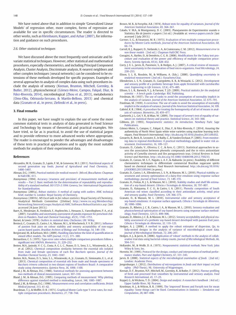
Fig. 6. Simulated scores for a sensory analysis of a new product development based on a scale ranging from0 to 100% of acceptance, overlaidwith a ND curve forx = 57.88 and s = 17.51.The SW test for normality gives p = 0.045 b 0.050; thus the hypothesis of normality of the data is rejected.
142 D. Granato et al. / Food Research International 55 (2014) 137–149
2.2. Parametric statistics in Food Science
Depending on the statistical distribution of data, sample size, andhomoscedasticity, samples and treatments can be compared using para-metric or non-parametric tests. Parametric tests should be used whendata are normally distributed and there is homogeneity of variances,as shown by the Shapiro–Wilk and Levene (or F) tests, respectively.
Fig. 7. Statistical steps and tests to compare two or more s
Then, a Student's t-test is used to check for differences between twomean values or an ANOVA is used when three or more mean valuesneed to be compared (Fig. 7).
2.2.1. Comparing two samples/treatmentsWhen the mean values for a specific characteristic in two data sets
are to be compared and both data sets are normally distributed and
amples in relation to a quantitative response variable.

143D. Granato et al. / Food Research International 55 (2014) 137–149
have similar variance, a Student's t-test should beused. The null hypoth-esis (H0) is that themean values donot differ; the alternative (Ha) is thatthey dodiffer. However, if there aremore than twodata sets it is not cor-rect to test each pair using a t-test (one of us recently received a paper inwhich 21 t-tests had been applied to compare individual pairs for sevensets of data!). The approach to be taken depends on whether the dataare paired or independent and it is sometimes difficult to choose thecorrect version of the test. Samples are considered to be independentwhen they differ in nature and do not depend on one another. Forexample, Student's t-test for independent samples should be used tocompare the ascorbic acid content of two cultivars of strawberries, orthe production of an enzyme by two bacterial strains. A paired samplet-test is used if each of several samples are analyzed in parallel for thesame characteristic by two different methods or if tests (e.g. bloodsugar levels) are done on samples taken from subjects both before andafter ingestion of a specific food ingredient. If the variances are notstrictly equal, a correction factor (Welch's test) should be included inthe statistical analysis. If the data do not conform to ND, non-parametric tests should be used.
2.2.2. Analysis of variances for three or more data setsAnalysis of variances (ANOVA) is a parametric statistical tool that
partitions the observed variance into components that arise fromdiffer-ent sources of variation. In its simplest form, ANOVA provides a statisti-cal test of whether or not the means of several groups are all equal. Inthis sense, the null hypothesis, H0, says there are no differencesamong results from different treatments or sample sets; the alternativehypothesis (Ha) is that the results do differ. If the null hypothesis isrejected then the alternative hypothesis, Ha, is accepted, i.e. at leastone set of results differs from the others. The ANOVA procedure shouldbe used to compare the mean values of three or more data sets. Onepractical example of application of analysis of variance is provided byOroian, Amariei, Escriche, and Gutt (2013): authors investigated therheological behavior of honeys from Spain under different temperatures(25 °C, 30 °C, 35 °C, 40 °C, 45 °C, and 50 °C) and concentrations andcompared the samples using one-way ANOVA followed by a test ofmultiple comparison of means.
Three alternative models can be used in an ANOVA: fixed effects,random effects or mixed effects models. The fixed effects model is ap-propriate when the levels of the independent variables (factors) areset by the experimental design. The random effects model, which isoften of greatest interest to a researcher, assumes that the levels ofthe effects are randomly selected from an infinite population of pos-sible levels (Calado & Montgomery, 2003). Independent variablesmay occur at several levels and it may be necessary to choose ran-domly only some levels; for instance, when samples are obtainedrandomly from four out of ten retailers of a particular product, orwhen three out of a possible seven brands of product are selectedfor analysis, provided always that the selection is done randomly.In certain circumstance some independent variables are assumedto be random effects and others to be fixed effects; here a mixedmodel should be used. In most experimental work a random effectsmodel approach is often the most appropriate.
Depending on the number of factors to be analyzed, we canhave:
1) A one-way ANOVA in which only one factor is assessed. This is thecase for relatively simple comparisons of physicochemical, colori-metric, chemical and microbiological analytes (Alezandro, Granato,Lajolo, & Genovese, 2011; Corry, Jarvis, Passmore, & Hedges, 2007;Granato &Masson, 2010; Oroian, 2012). For example, if five samplesof apple are analyzed for catechin content, the “apples” are the inde-pendent variable and the “catechin content” is the dependent re-sponse variable. Another important application of one-way ANOVAis when different groups of test animals that are treated with anextract/drug and compared to a control group (Macedo et al., 2013).
2) A 2-way ANOVA is used for two factors in which only the main ef-fects are analyzed. The 2-way ANOVA determines the differencesand possible interactions when response variables are from two ormore categories. The use of 2-way ANOVA enables comparison andcontrast of variables resulting from independent or joint actions(MacFarland, 2012). This type of ANOVA can be employed in sensoryevaluation when both panelists and samples are sources of variation(Granato, Ribeiro, & Masson, 2012) or when the consistency of thepanelists needs to be assessed;
3) A factorial ANOVA for n factors, that analyzes themain and the inter-action effects is themost usual approach formany experiments, suchas in a descriptive sensory ormicrobiological evaluation of foods andbeverages (Ellendersen, Granato, Guergoletto, & Wosiacki, 2012;Jarvis, 2008; Mon & Li-Chan, 2007);
4) A repeated-measures (RM) ANOVA is used to analyze designs inwhich responses on two ormore dependent variables correspondto measurements at different levels of one or more varyingconditions. Benincá, Granato, Castro, Masson, and Wiecheteck(2011) used a RM-ANOVA to examine results from assessmentsof different instrumental color attributes for a mixture of juicesfrom yacón (Peruvian ground apple) tubers and yellow passionfruit as a function of storage time.
The ANOVA approach provides a global analysis of the overall vari-ance and assesses whether or not the variance of one or more, datasets differs significantly from the others but the output does not identifywhich variables differ. Thus, post-hoc tests need to be performed inorder to specify exactly which pairs of means differ statistically. Variousparametric and non-parametric tests can be used to compare themeansof response variables, based on a normal or non-normal distribution ofmeans, respectively. The choice of post-hoc tests to be used should bedecided in advance so that bias is not attributed to any one set of data.
In recent times, so-called ‘robust’ ANOVA methods have been devel-oped that are not affected by outlier data and can be used when data donot conform strictly to ND. Theywere developed following a need to an-alyze inter-laboratory studies during validation of analyticalmethods foruse in chemistry andmicrobiology and are important also in determina-tion of measurement uncertainty estimates that are nowadays requiredas part of laboratory accreditation (Elison, Rosslein, & Williams, 2000).Two approaches have been described: the first (Anonymous, 2001a) isbased on a recursive application of an M-type estimator (Barnet &Lewis, 1978) and the second uses theMedian Absolute Paired Deviation(MAPD) described originally by Rousseuux and Croux (1993). For expla-nation of these procedures refer to Hedges and Jarvis (2006) andHedges(2008). Software for the MAD procedure can be downloaded from theAnonymous (2001b).
2.2.3. Post-hoc tests to compare three or more samples/treatmentsPost-hoc tests are used for investigation of statistically significant dif-
ferences (pANOVA b 0.05) identified in an analysis of variance. When themean values of three ormore samples have homogeneous variances, theperformance of such post-hoc tests in terms of Type I error (acceptingequality of means when they are actually different) and Type II error(rejecting equality when they are not different) has been evaluated bymany workers including Gabriel (1964), Boardman and Moffitt (1971),O'Neill and Wetheril (1971), Bernardson (1975), Conagini, Barbin, andDemétrio (2008), but there are still manyunanswered questions regard-ing suitability. In practice, the choice of the best test to compare meanvalues depends on the investigator's experience. We recommend theuse of Duncan's multiple range test (MRT) or Fisher's Least SignificantDifference (LSD) test because of their high power to detect significantdifferences in mean values (Fig. 4) or Tukey's Honest Significant Differ-ence (HSD) test.
The Tukey HSD is a single-step multiple comparison generally usedin conjunction with an ANOVA to identify if one mean value differs sig-nificantly from another. It compares all possible pairs of means and is

Table 1Use of theWilcoxon Signed Ranks test to determine the level of patulin in lots of an applecompote (legal limit 25 μg/kg) using two analytical methods (A & B).
Production lot Patulin (μg/kg) Difference Sign Rank (R) Signed R
A B A − B
1 12.5 10.5 2.0 + 8.5 +8.52 11.5 10.8 0.7 + 6 +63 12.5 13.0 −0.5 − 4 −44 12.0 12.0 0 − −5 14.0 12.0 2.0 + 8.5 +8.56 12.5 12.4 1.0 + 1 +17 14.0 12.3 1.7 + 7 +78 12.5 12.7 −0.2 − −2 −29 14.0 13.5 0.5 + 4 +410 13.0 12.5 0.5 + 4 +4Mean 12.85 12.17 Sum R+ +39
Sum R− −6
Tabulate the results for methods A & B, then determine the difference (A − B).Ignoring the sign and any zero value allocate a rank to each difference, using an averagerank if results are identical. Then allocate the relevant sign to each rank.Add the rank scores for R+ and R− and, for the number of pairs (in this case n = 9),compare the smaller rank total with the tabulated value in tables of Wilcoxon's signedranks. If, as in this case, the smaller rank total is ≤ published value then the difference isstatistically significant at p = 0.05. Hence the null hypothesis, that results from bothmethods are equal, should be rejected as method A gives higher results. Whether the dif-ferences are of practical importance is another matter!
144 D. Granato et al. / Food Research International 55 (2014) 137–149
the most useful test for multiple comparisons. However, the method isnot statistically robust, being sensitive to the requirement that themeans need to follow a normal distribution. Evenwhen there is a signif-icant difference between a pair of means, this test often does not pin-point it (Calado & Montgomery, 2003). However, many researchersclaim that the Tukey test is the procedure of choice since it avoidsType II errors.
Fisher's LSD test is a statistical significance test used where sam-ple sizes are small and when the distribution of the residues is nor-mal (pLevene ≥ 0.05). The test is much more robust than Tukey butit is the most sensitive to Type I errors; yet it provides an importanttool for comparing means after an ANOVA procedure (Carmer &Swanson, 1973). Duncan's MRT is not restricted to data conformingstrictly to ND and does not require a significant overall ‘between-treatments’ F test but it is also likely to give Type I errors. TheTukey–Kramer HSD single-step multiple comparison procedurecompares mean values using a ‘Studentized Range’, which is moreconservative than the original Tukey HSD test, and can be usedwith unequal group sizes. It is much stricter than many other testsbut is less likely to give Type I errors (Keppel & Wickens, 2004).
2.3. Non-parametric statistics in Food Science
Non-parametric procedures use ranked data rather than actual datavalues. The data are ranked from the lowest to the highest and eachvalue is assigned, in order, the integer values from 1 to n (wheren = total sample size) (Hollander & Wolfe, 1973). Non-parametricmethods provide anobjective approachwhen there is no reliable (univer-sally recognized) underlying scale for the original data andwhen there isconcern that the results of standard parametric techniqueswould be crit-icized for their dependence on an artificial metric (Siegel, 1956). Suchtests have the obvious advantage of not requiring any assumption of nor-mality or homogeneity of variance. Because they comparemedians ratherthanmeans the comparison is not influenced by outlier values. Themajordisadvantage of non-parametric techniques is the lack of defined param-eters and it is more difficult to make quantitative statements about theactual difference between populations. Ranking for non-parametric pro-cedures preserves information about the order of the data but discardsthe actual values. Because information is discarded, non-parametric pro-cedures can never be as powerful (i.e. less able to detect differences) astheir parametric counterparts (Hollander & Wolfe, 1973).
Non-parametric tests are also used for nominal, categorical and ordi-nal data or when data have been assigned values on an arbitrary scalefor which no definitive numerical interpretation exists, such as whenevaluating preferences in sensory evaluation. Every non-parametricprocedure has its peculiar sensitivities and blind spots. If possible, it isalways advisable to run different nonparametric tests; if there are dis-crepancies in the results, one should try to understand why certaintests give different results.
2.3.1. Comparing two samples/treatmentsNon-parametric tests can be used to examine data in a manner that
is analogous to the use of paired and independent t-tests. Independenttests are evaluated using the Mann–Whitney test (Mann & Whitney,1947) and paired tests by the Wilcoxon signed rank tests. Both requireranking of data as the first stage of the evaluation.
In what way are data unsuitable for parametric testing? Choice ofnon-parametric tests is predicated on examination of data that do notconform to a ND, especially data from samples drawn from differentpopulations. For example, consider the comparison of a new simplemethod (B) with a standard method (A) for estimation of patulin insamples of an apple pureemanufactured at different times from a num-ber of individual ingredient sources. Since all ingredients come fromdif-ferent populations and the products are prepared individually, samplestaken from any one ‘lot’ would come from a unique population butacross ‘lots’ each populationwould be different. Since the same samples
are tested by the two methods it is appropriate to consider the tests tobe paired but as each sub-set of analyses is made on a different popula-tion of samples it is not appropriate to use a Student's t-test. Themethodof choice is theWilcoxon Signed Ranks test (Wilcoxon, 1945)where thedifference between the results for the twomethods (A, B) is determinedand a sign (+,−) is used to definewhethermethodAor B is the greater.Values are then ranked in sequence from the smallest value upwardsbut without reference to the sign; the sign is then reinstated againstthe rank value and the sums of the + and − ranks are determined(Table 1). The lesser rank total is then compared with tabulated valuesfor theWilcoxon signed rank statistic (U) and the statistical significanceis determined.
Another example might be where two independent methods havebeen used to swab chicken skins for levels of bacteria. Each area willbe independent of all other areas and the two swabbing proceduresare also completely independent. Once again we are dealing with non-normal populations from discrete work areas so we cannot use para-metric tests to compare the results. In this case the procedure of choiceis theMann–Whitney U test. If we assume that there are n pairs of tests,ranks are allocated from 1 to 2n without regard for the data set fromwhich they come (Table 2). The total rank scores for each method arethen determined and a U statistic is calculated for each data set. Thesmaller value of U is then compared with tabulated values to determinethe significance.
Full details of these tests, together with tables of significant values,are found in standard texts such a Snedecor & Cochrane (1989).
2.3.2. Comparing three or more samples or treatmentsItwill have beennoted above that the key requirement for a paramet-
ric comparison of three or more variables using ANOVA is that the datamust conform to, or be transformable, to a ND and the variances shouldbe relatively homogeneous. If this is not possible, two non-parametricapproaches can be used: the Kruskal–Wallis and the Friedman tests.Both tests rely on ranking of results but whilst the Kruskal–Wallis testranks all results (with ties getting the average rank) before summatingthe rank values according to the treatment, in the Friedman test ranksare determined for each individual treatment.
The Kruskal and Wallis (1952) is a non-parametric multiple rangetest of differences in central tendency (median) that essentially pro-vides a one-way analysis of variance for three or more independentsamples based on ranked data. It is most often used for analysis of

Table 2Comparison of bacterial numbers on cotton and plastic sponge swabs taken from chickenneck skins immediately after evisceration.
Number of bacteria (CFU × 10−4/25 cm2)
Cotton swab (A) Sponge swab (B)
Count Rank Count Rank
110 14.5 20 716 6 200 2024 8 5 2105 13 89 11155 18 125 162 1 140 17104 12 180 1910 4 49 107 3 15 528 9 110 14.5
Allocate ranks (1–20) across both sets of data; average the rank for identical counts (in thiscase, counts of 110).Calculate the rank totals: RA = 88.5; RB = 121.5.Calculate the UA statistic for data set A: UA = [nA(nA + 1) / 2 + nAnB − RA] = 66.5.Similarly, calculate the UB statistic for data set B: UB = 33.5.Take the smaller value of U as the test statistic and compare it with the Mann–Whitneytabulated value for p = 0.05 with nA = nB = 10.The calculated value of UB (33.5) N Ucritical (23) so the null hypothesis that both methodsgive equal results is not rejected — the 2-tailed probability is p = 0.25.
Table 3Non-parametric analysis of the scores from a wine tasting.
Wine Score for taster no.
1 2 3 4 5
A 1 1 2 1 3B 5 5 4 5 5C 2 3 3 1 3D 1 3 1 3 2E 1 2 1 2 2F 2 2 2 4 2
Table 4Average rank for the wine tasters.
Wine (n) Ranked score for taster (k)
1 2 3 4 5
A 2 2 4 2 5B 3.5 3.5 1 3.5 3.5C 2 4 4 1 4D 1.5 4.5 1.5 4.5 3E 1.5 4 1.5 4 4F 2.5 2.5 2.5 5 2.5Total (Rk) 13 20.5 14.5 20 22Rk
2 169.0 420.3 210.3 400.0 484.0
145D. Granato et al. / Food Research International 55 (2014) 137–149
data having one ‘nominal’ variable and one ‘continuous’ variable. An ex-ample of its use might be the case of a food engineering study in whichthree different brands of filter pads are tested to assess their effective-ness in filtering beer. Replicate filters of each brand are assessed usingone batch of raw beer to determine the period of time before each filterbecomes blocked (as judged by e.g. the filter pressure); thework is thenrepeated on further batches of beer. The objective is to assess the cost-effectiveness of the different brands. The filter brands provide the ‘nom-inal’ values and the time to blocking is the continuous measurement.The test can be used for data with non-homogeneous variances or fordata that do not conform to ND; it can be used when the groups are ofunequal size, but the test assumes that the shape and distribution ofdata for each group is similar. The test is essentially an extension ofthe Mann–Whitney U test (qv), which can be applied to pairs of dataas a post-hoc test of significance between pairs of results.
The Friedman (1937, 1939) test is used to determine differences incentral location (median) for analysis of trials with one-way repeatedmeasures having three or more dependent samples and is also basedon ranking of data. Dependent samples might include, for instance,the assessment scores of k taste panelists who are judging n indepen-dent samples of wine— are the scores given by each panelist consistentor is there a significant difference between panelists and, if so, does thisdiffer between the wine samples? The data consists of a matrix of nrows (the ‘blocks’) representing the wine samples and k columns(treatments) representing the panelists. Five trainee wine tasters haveassessed the overall quality of each of six wines, using hedonic scoresfrom 1 (excellent) through 3 (average) to 5 (awful). The results aresummarized in Table 3. The data for each ‘block’ are ranked from lowestto highest, tied values each being given the average rank. The rankeddata are then analyzed to determine the χ2 value. If the null hypothesisthat themean scores do not differ is rejected it is then necessary to carryout post-hoc tests to determine the source(s) of the differences.
Recognizing that some variation in response is to be expected, theinstructor wishes to knowwhether there is overall agreement betweenthe tasters. The approach is to use the Friedman procedure that ranksthe performance of tasters for each wine. If the taste score betweentwo or more individuals is identical each receives the average rank inTable 4.
The scores for each taster are totaled (Rk) and the square of thetotals is determined (Rk
2). The number of tasters = k = 5; the
number of samples = n = 6. We determine a value M using the
equation: M ¼ 12nk kþ1ð Þ∑R2
k−3n kþ 1ð Þ.For these data,M = 4.233withυ = k − 1 = 4degrees of freedom.
From the Tables, we find that the critical value for χ2(p = 0.05, υ = 4) is9.49 which is greater than M and therefore we do not reject the nullhypothesis that the tasters have scored the samples uniformly.
Full details of these, and other nonparametric and parametric tests,are given in standard works including Sheskin (2011).
2.4. Bivariate correlation analysis
Correlation is a method of analysis used to study the possible associ-ation between two continuous variables. The correlation coefficient (r)is a measure that shows the degree of association between both vari-ables (Granato, Calado, Oliveira, & Ares, 2013). This parametric test re-quires both data sets to consist of independent random variables thatconform to ND. The correlation coefficientmeasures the degree of linearassociation between the two sets of data (A and B), and its value liesbetween−1 and+1. The closer the absolute value, |r|, is to 1, the stron-ger the correlation between the data values (Ellison, Barwick, & Farrant,2009). The correlation between two variables is positive (Fig. 8A) if highvalues for one variable are associatedwith high values for the other var-iable and negative (Fig. 8B) if one variable is lowwhen the other is high.A correlation close to r = 0 (Fig. 8C) indicates that there is no linearrelation, or at best a very weak correlation, between the two variables.However, a low r-value does not necessarily imply that there is no rela-tionship between the responses; a low value can be due to the existenceof a non-linear correlation between these variables, but the presence ofoutliers in one or both data sets may also affect the r-value (Altman,1999).
Many workers calculate the Pearson linear correlation coefficient inorder to seek to determine the strength of association between datasets. However, whenmore than five variables are analyzed, the analysisis compromised because correlation coefficients do not assess simulta-neous association among results for all variables, which makes it diffi-cult to understand and interpret the structure and patterns of thedata. For example, if one considers five sets of response variables (A, B,C, D and E), it is necessary to calculate the correlation coefficients, andtheir significance, for each data set pair, i.e. AB, AC, AD, AE, BC, BD, BE,CD, CE, and DE. It is easy to understand and interpret up to three

146 D. Granato et al. / Food Research International 55 (2014) 137–149
correlations coefficients but, in order to better understand multiple re-sponses, a more sophisticated multivariate statistical approach, suchas principal component analysis, clustering techniques, linear discrimi-nant analysis should be used (Besten et al., 2012, 2013; Granato et al., inpress; Zielinski et al., in press).
When large sets of results (≥30) are analyzed, data should be for-mally checked for normality. If the data do not follow a normal distribu-tion a non-parametric approach, such as the Spearman's rank correlationcoefficient, should be used to analyze for any correlation between theresponses. Fig. 9 shows the steps to follow when two data sets (eachwith n ≥ 8) are to be analyzed with respect to correlation. Spearman'scorrelation coefficient (ρ) should be used when either or both datasets do not conform to ND, when the sample size is small, or when thevariables are measured as ordinals i.e. first, fifth, eighth, etc. in a se-quence of values. The Spearman correlation coefficient does not requirethe assumption that the relationship between variables is linear.
One good example to compare both Pearson and Spearman correla-tion coefficients can be obtained by analyzing the data sets below:
A: 12.56; 14.46; 16.65; 25.68; 16.80; 28.95; 32.25; 30.33; 32.81;28.29; 29.98; 30.32; 33.57
0
2
4
6
8
10
12
14
16
18
20
Var
iab
le B
Variable A
0
5
10
15
20
25
Var
iab
le B
Variable A
0
5
10
15
20
25
0 2 4 6 8 10 12 14 16
Var
iab
le B
Variable A
C
B
A
0 2 4 6 8 10 12 14 16
0 2 4 6 8 10 12 14 16
Fig. 8. (A) Positive correlation, (B) negative correlation, and (C) almost null correlation.
B: 53.25; 65.33; 53.68; 62.74; 61.53; 64.89; 66.40; 60.99; 68.50;56.30; 66.36; 68.25; 73.89.
The normality of both data sets was assessed using the Shapiro–Wilktest and p-values of 0.017 and 0.605 were obtained for A and B, respec-tively. Since onedata set does not followanormal distribution, Spearmancorrelation rank coefficient (ρ = 0.753, p = 0.004) should be used rath-er than the Pearson correlation coefficient (r = 0.660, p = 0.014). Asobserved in this simple example, it is possible to assume that dependingon the method employed to assess correlation between two responsevariables, the coefficient magnitude and its significance may be highlydifferent, and the conclusion (inferences) of the studymay bemisleadingor even wrong.
There is no scientific consensus about the qualitative assessment ofcorrelation coefficients, that is, whether a correlation coefficient istruly strong, moderate or weak. Granato, Castro, Ellendersen, andMasson (2010) established an arbitrary scale for the strength of correla-tions between variables using the following criteria: perfect (|r| = 1.0),strong (0.80 ≤ |r| b 1.0), moderate (0.50 ≤ |r| b 0.80), weak(0.10 ≤ |r| b 0.50), and very weak (almost none) correlation(0.10 ≤ |r|).
There are two major concerns regarding correlation tests: the signifi-cance of the correlation and the interpretation of results. Firstly, to as-sume a statistically significant association between variables the p-valueof the correlation coefficient should be b0.05. Granato, Katayama, andCastro (2011) showed thatwith large data sets, the correlation coefficientis often statistically significant even at a moderate or low r value. On theother hand,when the data set is small (Granato, Freitas, &Masson, 2010),high values of rmay be observed but the statistical probability of the cor-relation is not significant (p N 0.05). Secondly, when a correlation coeffi-cient is calculated, it is not always possible to assume causation because
Fig. 9. Steps to follow when two data sets (usually with n ≥ 8) are to be analyzed forcorrelation.

147D. Granato et al. / Food Research International 55 (2014) 137–149
co-variants may contribute to the response, i.e. correlated occurrencesmay be due to a common cause. For example, suppose one researcher,studying the effects of increasing sugar levels on the sensory acceptanceof coffee using a consumer panel, obtains a correlation coefficient of+0.72 with p = b0.05 but another researcher in another place, usingthe same trial conditions repeats the test and obtains very different corre-lation coefficients and probability value. The explanation is possibly relat-ed to differences in consumer habits and experience but might alsoreflect the variety and composition of the coffee beans, their roastingand the preparation of coffee for the test. Hence, although correlationstudies can be extremely useful, they do not automatically imply acause and effect relationship between the variables. Another aspect ofcorrelation that often needs to be considered is the intra-class correlationcoefficient. This provides a measure of the correlation between two setsof variables when the data are paired or can be organized into groups. Itis analogous to the use of a paired, rather than an independent, t-test.The procedure, described in Bland and Altman (1996), estimates the pro-portion of total variance that is due to the between-group component; ithas many applications but is particularly useful for examination of tastepanel results from examination of replicate samples of a product.
Although a correlation coefficient provides ameasure of the strengthof a relationship between two sets of data, it does not prove equivalencebetween the results. Lack of equivalence is due to bias and can be deter-mined using the Bland and Altman (1986, 1995) procedure. For exam-ple, comparison of two analytical methods may give results that arehighly correlated but when bias is assessed, one method may give con-sistently larger or smaller values for the same set of samples; thus thetwo methods do not provide equivalent results.
2.5. Regression analysis
Regression analysis is used to examine the relationship betweensets of dependent and independent variables and includes manytechniques for modeling and analyzing two or more sets of data.There are many forms of regression including linear, multi-linear,probit and logistic approaches, the latter being particularly impor-tant in studying biological responses to dose levels of inhibitory orstimulatory treatments. In its simplest form, regression is used to as-sess the relative effects of e.g. increasing treatment times (or tem-peratures) on the heat resistance of microorganisms in order todetermine thermal effects (D-values) under defined process condi-tions. It may be used also to establish calibration curves for chemical,physical and biological assays for continuous data sets. Calibrationcurves require at least five concentration levels including a blankvalue with adequate (at least triplicate) replication of tests at eachconcentration level.
Assumptions for regression require that:
– The samples are representative of the population for the inferenceprediction;
– The concentrations of the independent variables are measured withzero error, i.e. they are ‘absolute’ values; if this is not the case thenthe more complex orthogonal linear regression must be used inorder to correct for errors in the predictor variable (cf. Carroll,Ruppert, Stefanski, and Crainiceanu (2012)
– The error term of the estimates is a randomvariablewith zeromean;– The predictors are linearly independent, i.e. each value cannot be
expressed as a linear combination of the other values;– The variance of the errors is homoscedastic.
In order to perform a regression analysis it is essential to:
– Test data for the presence of outliers (at 95 or 99% of confidence)using the Grubb's test for each concentration level;
– Ensure the homogeneity of variances in the concentration levelsof the calibration curve by using one the tests described above(Section 2.1.2).
– Build the model (i.e. the graph) to display the analyte concentra-tion versus the response (absorbance, area, etc.);
– Test the significance of the regression and its lack of fit throughthe F-test and a one-factor ANOVA. Provided that the responseis directly and linearly correlated to the concentrations then theregression coefficient should be significant. Evidence for lack offit (p b 0.05), may be due to a non-linear response, to excessivevariation in the replicates at one or more of the test values orthe use of an over-extended independent variable range. In thiscase, removing the highest values and repeating the statisticalanalysis should reduce the range of concentrations. Evidence forlack of linearity may indicate that a nonlinear model (quadratic,for example) might be more appropriate for the method, andtherefore, alternative models should be evaluated.
– Determine the following statistical parameters by means of theregression analysis:• The regression equation (y = ax + b), where y is the dependentestimate at independent concentration level (x), a is the slope ofthe line and b is the linear intercept when x = 0;
• The standard deviation of the estimated parameters and model;• The statistical significance of the estimated parameters;• The coefficient of determination (R2; regression coefficient) andthe adjusted R2.
The regression model is considered suitable to the experimentaldata when:
1. The standard deviation of the parameter is at least 10% lower thanthe corresponding parameter value;
2. The standard deviation of theproposedmathematicalmodel is small;3. The parameters of amodel are statistically significant otherwise they
will not contribute to the model.
It is a myth to consider that if R2 N 90% the model is excellent(Montgomery & Runger, 2011). This is only one criterion to evaluatethe goodness of fit of the model. If R2 is low (b70%), the mathematicalmodel is not good; on the other hand, if R2 is high (N90%), it meansthat you should continue the analysis and check the other criteria. It isnoteworthy that in some applications, depending on the type of analy-sis, e.g. evaluation of sensory data, the coefficient of determinationmay be considered good if R2 N 60%;
4. The statistical significance, obtained from the F-test of an ANOVAanalysis of the proposed mathematical model is at least p b 0.05;
5. Analysis of the residuals (experimental value for a response var-iable minus value predicted by the mathematical model) mustconform to ND and have a constant variance, as describedabove. This is a necessary condition for the application of somepost-hoc tests such as t and F.
It is important to recognize that the regression and correlation coeffi-cients describe different parameters. Regression describes the goodnessof fit of a model; correlation estimates the linear relationship of twovariables.
A common mistake is to use R2 to compare models. R2 is alwayshigher if we increase the order of a model (linear in comparison to qua-dratic, for example). For example, a third order polynomial has a higherR2 than a second order polynomial because there are more terms, but itdoes not necessarily mean that the first is the better model. An analysisof the degrees of freedom (number of experimental points minus num-ber of parameters from the model) needs to be carried out. A modelwith more terms requires estimation of more coefficients so fewer de-grees of freedom remain. Thus, another criterion needs to be used: theadjusted regression coefficient — Radj
2 . This coefficient adjusts for thenumber of explanatory terms in a model relative to the number ofdata points and its value is usually less than or equal to that of R2.When comparing models, the one with the highest adjusted coefficientis the best model.
148 D. Granato et al. / Food Research International 55 (2014) 137–149
We have noted above that in addition to simple ‘Generalized LinearModels’ of regression other, more complex, forms of regression areavailable for use in specific circumstances. The reader is directed tootherworks, such as Kleinbaum, Kupper, andAzhar (2007), for informa-tion and guidance on such procedures.
2.6. Other statistical techniques
Wehave discussed above themost frequently used univariate and bi-variate statistical techniques. However, other statistical andmathematicalprocedures, especially chemometrics, and including Principal ComponentAnalysis, Cluster Analysis, Discriminate analysis, K-nearest neighbors andother complex techniques (neural networks) can be considered to be ex-tensions of these methods developed for specific purposes. Examples ofseveral approaches to analysis of complex data using such procedures in-clude the analysis of sensory (Keenan, Brunton, Mitchell, Gormley, &Butler, 2012), physicochemical (Gómez-Meire, Campos, Falqué, Díaz, &Fdez-Riverola, 2014), microbiological (Zhou et al., 2013), metabolomics(Oms-Oliu, Odriozola-Serrano, & Martín-Belloso, 2013) and chemicaldata (Granato et al., in press; Zielinski et al., in press).
3. Final remarks
In this paper, we have sought to explain the use of some the morecommon statistical tests in analysis of data generated in Food Scienceand Technology by means of theoretical and practical examples. Wehave tried, so far as is practical, to avoid the use of statistical jargonand to provide reference to more advanced works where appropriate.The reader is encouraged to ponder the advantages and disadvantagesof these tests in practical applications and to apply the most suitablemethods for analysis of their experimental data.
References
Alezandro, M. R., Granato, D., Lajolo, F. M., & Genovese, M. I. (2011). Nutritional aspects ofsecond generation soy foods. Journal of Agricultural and Food Chemistry, 59,5490–5497.
Altman, D.G. (1999). Practical statistics for medical research (8th ed.)Boca Raton: Chapman& Hall/CRC, 611.
Anonymous (1994). Accuracy (trueness and precision) of measurement methods andresults — Part 2: Basic methods for the determination of repeatability and reproduc-ibility of a standardmethod. ISO 5725-2:1994. Geneva, Sw: International Organizationfor Standardisation.
Anonymous (2001a). Robust statistics: A method of coping with outliers. AMC technicalbrief, number 6. London: Royal Society of Chemistry.
Anonymous (2001b).MS Excel add-in for robust statistics: Royal Society of Chemistry,Analytical Methods Committee ([Online] http://www.rsc.org/Membership/Networking/InterestGroups/Analytical/AMC/Software/RobustStatistics.asp (lastaccessed 24 June 2013))
Baert, K., Meulenaer, B., Verdonck, F., Huybrechts, I., Henauw, S., Vanrolleghem, P. A., et al.(2007). Variability and uncertainty assessment of patulin exposure for preschool chil-dren in Flanders. Food and Chemical Toxicology, 45(9), 1745–1751.
Barnet, & Lewis (1978). Outliers in statistical data. Chichester, UK: Wiley.Benincá, C., Granato, D., Castro, I. A., Masson, M. L., &Wiecheteck, F. V. B. (2011). Influence
of passion fruit juice on colour stability and sensory acceptability of non-sugaryacon-based pastes. Brazilian Archives of Biology and Technology, 54, 149–159.
Bergstrand, M., & Karlsson, M.O. (2009). Handling data below the limit of quantification inmixed effect models. The AAPS Journal, 11(2), 371–380.
Bernardson, C. S. (1975). Type error rates whenmultiple comparison procedures follow asignificant test ANOVA. Biometrics, 31, 229–232.
Besten, M.A., Jasinski, V. C. G., Costa, A. G. L. C., Nunes, D. S., Sens, S. L., Wisniewski, A., Jr.,et al. (2012). Chemical composition similarity between the essential oils isolatedfrom male and female specimens of each five Baccharis species. Journal of theBrazilian Chemical Society, 23, 1041–1047.
Besten, M.A., Nunes, D. S., Sens, S. L., Wisniewski, A., Jr., Granato, D., Simionatto, E. L., et al.(2013). Chemical composition of essential oils from male and female specimens ofBaccharis trimera collected in two distant regions of Southern Brazil: A comparativestudy using chemometrics. Quimica Nova, 36, 1096–1100.
Bland, J. M., & Altman, D.G. (1986). Statistical methods for assessing agreement betweentwo methods of clinical measurement. Lancet, 307–310.
Bland, J. M., & Altman, D.G. (1995). Comparing methods of measurement: Why plottingdifference against standard method is misleading. Lancet, 346, 1085–1087.
Bland, J. M., & Altman, D.G. (1996). Measurement error and correlation coefficients. BritishMedical Journal, 313, 41–42.
Boardman, T. J., & Moffitt, D. R. (1971). Graphical Monte Carlo type Y error rates, for mul-tiple comparison procedures. Biometrics, 27, 738–744.
Brown, M. B., & Forsythe, A.B. (1974). Robust tests for equality of variances. Journal of theAmerican Statistical Association, 69, 364–367.
Calado, V. M.A., & Montgomery, D. C. (2003). Planejamento de Experimentos usando oStatistica. Rio de Janeiro: e-papers (1st ed.) (Available at: www.e-papers.com.br (lastaccessed 2 July 2013))
Carmer, S. G., & Swanson, M. R. (1973). Evaluation of ten multiple comparison proce-dures by Monte Carlo methods. Journal of the American Statistical Association, 68,66–74.
Carroll, R. J., Ruppert, D., Stefanski, L. A., & Crainiceanu, C. M. (2012).Measurement error innon-linear models (2nd ed.): Chapman Hall/CRC Press.
Conagini, A., Barbin, D., & Demétrio, C. G. B. (2008). Modifications for the Tukey test pro-cedure and evaluation of the power and efficiency of multiple comparison proce-dures. Scientia Agricola, 65(4), 428–432.
Corry, J. E. L., Jarvis, B., Passmore, S., & Hedges, A. J. (2007). A critical review of measure-ment uncertainty in the enumeration of foodmicro-organisms. FoodMicrobiology, 24,230–253.
Elison, S. L. R., Rosslein, M., & Williams, A. (Eds.). (2000). Quantifying uncertainty inanalytical measurement (2nd ed.): Eurachem/Citac.
Ellendersen, L. S. N., Granato, D., Guergoletto, K. B., & Wosiacki, G. (2012). Developmentand sensory profile of a probiotic beverage from apple fermented with Lactobacilluscasei. Engineering in Life Sciences, 12(4), 475–485.
Ellison, S. L. R., Barwick, V. J., & Farrant, T. J.D. (2009). Practical statistics for the analyticalscientist — A bench guide. Cambridge: RSC Publishing.
Friedman, M. (1937). The use of ranks to avoid the assumption of normality implicit inthe analysis of variance. Journal of the American Statistical Association, 32, 675–701.
Friedman, M. (1939). A correction: The use of ranks to avoid the assumption of normalityimplicit in the analysis of variance. Journal of the AmericanStatistical Association, 34, 109.
Gabriel, K. R. (1964). A procedure for treating the homogeneity of all set of means in anal-ysis of variance. Biometrics, 20, 459–477.
Gastwirth, J. L., Gel, Y. R., & Miao,W. (2009). The impact of Levene's test of equality of var-iances on statistical theory and practice. Statistical Science, 24, 343–360.
Gibbons, J.D. (1993). Nonparametric statistics: An introduction. Newbury Park: SagePublications.
Gómez-Meire, S., Campos, C., Falqué, E., Díaz, F., & Fdez-Riverola, F. (2014). Assuring theauthenticity of North West Spain white wine varieties using machine learning tech-niques. Food Research International. http://dx.doi.org/10.1016/j.foodres.2013.09.032.
Govaerts, B., Beck, B., Lecoutre, E., le Bailly, C., & Vanden Eeckaut, P. (2005). Frommonitor-ing data to regional distributions: A practical methodology applied to water risk as-sessment. Environmetrics, 16, 109–127.
Granato, D., Calado, V., Oliveira, C. C., & Ares, G. (2013). Statistical approaches to as-sess the association between phenolic compounds and the in vitro antioxidantactivity of Camellia sinensis and Ilex paraguariensis teas. Critical Reviews in FoodScience and Nutrition. http://dx.doi.org/10.1080/10408398.2012.750233.
Granato, D., Caruso, M. S. F., Nagato, L. A. F., & Alaburda (in press). Feasibility of differentchemometric techniques to differentiate commercial Brazilian sugarcane spiritsbased on chemical markers. Food Research International. http://dx.doi.org/10.1016/J.FOODRES.2013.09.044 (in press).
Granato, D., Castro, I. A., Ellendersen, L. S. N., & Masson, M. L. (2010). Physical stability as-sessment and sensory optimization of a dairy-free emulsion using response surfacemethodology. Journal of Food Science, 73, 149–155.
Granato, D., Freitas, R. J. S., & Masson, M. L. (2010). Stability studies and shelf life estima-tion of a soy-based dessert. Ciência e Tecnologia de Alimentos, 30, 797–807.
Granato, D., Katayama, F. C. U., & Castro, I. A. (2011). Phenolic composition of SouthAmerican red wines classified according to their antioxidant activity, retail priceand sensory quality. Food Chemistry, 129, 366–373.
Granato, D., & Masson, M. L. (2010). Instrumental color and sensory acceptance ofsoy-based emulsions: A response surface approach. Ciência e Tecnologia de Alimentos,30, 1090–1096.
Granato, D., Ribeiro, J. C. B., Castro, I. A., & Masson, M. L. (2010). Sensory evaluation andphysicochemical optimisation of soy-based desserts using response surface method-ology. Food Chemistry, 121(3), 899–906.
Granato, D., Ribeiro, J. C. B., &Masson, M. L. (2012). Sensory acceptability and physical sta-bility assessment of a prebiotic soy-based dessert developed with passion fruit juice.Ciência e Tecnologia de Alimentos, 32, 119–125.
Hedges, A. J. (2008). A method to apply the robust estimator of dispersion, Qn, tofully-nested designs in the analysis of variance of microbiological count data.Journal of Microbiological Methods, 72, 206–207.
Hedges, A. J., & Jarvis, B. (2006). Application of ‘robust’ methods to the analysis of collab-orative trial data using bacterial colony counts. Journal of Microbiological Methods, 66,504–511.
Hollander, M., & Wolfe, D. A. (1973). Nonparametric statistical methods. New York: JohnWiley & Sons, Inc.
Horwitz,W. (1995). Protocol for the design, conduct and interpretation ofmethod perfor-mance studies. Pure and Applied Chemistry, 67, 331–343.
Jarvis, B. (2008). Statistical aspects of the microbiological examination of foods (2nd ed.)London: Academic Press.
Jongenburger, I. (2012). Distributions of microorganisms in foods and their impact on foodsafety. (PhD Thesis). NL: University of Wageningen.
Keenan, D. F., Brunton, N.P., Mitchell, M., Gormley, R., & Butler, F. (2012). Flavour profilingof fresh and processed fruit smoothies by instrumental and sensory analysis. FoodResearch International, 45, 17–25.
Keppel, G., & Wickens, T. D. (2004). Design and analysis: A researchers handbook (4rd ed.)Upper Saddle River, NJ: Pearson.
Keselman, H. J., & Wilcox, R. R. (1999). The ‘improved’ Brown and Forsyth test for meanequality: Some things can't be fixed. Communications in Statistics — Simulation andComputation, 28, 687–698.

149D. Granato et al. / Food Research International 55 (2014) 137–149
Kleinbaum, D., Kupper, L., & Azhar, N. (2007). Applied regression analysis and multivariatemethods (4th ed.) Thomson Brooks/Cole; Duxbury, Belmont, Ca, USA.
Kruskal, W. H., & Wallis, W. A. (1952). Use of ranks in one-criterion variance analysis.Journal of the American Statistical Society, 47, 583–621.
Levene, H. (1960). Robust tests for equality of variances. In I. Olkin (Eds.), Contributions toprobability and statistics: Essays in honor of Harold Hotelling (pp. 278–292): StanfordUniversity Press.
Lim, T. S., & Loh, W. Y. (1996). A comparison of tests of equality of variances.Computational Statistics and Data Analysis, 22, 287–301.
Lorrimer, M. F., & Kiermeier, A. (2007). Analyzing microbiological data — Tobit or notTobit? International Journal of Food Microbiology, 116, 313–318.
Macedo, L. F. L., Rogero, M. M., Guimarães, J. P., Granato, D., Lobato, L. P., & Castro, I. A.(2013). Effect of red wines with different in vitro antioxidant activity on oxidativestress of high-fat diet rats. Food Chemistry, 137, 122–129.
MacFarland, T. W. (2012). Two-way analysis of variance — Statistical tests and graphicsusing R. Springer, 150.
Mann, H. B., &Whitney, D. R. (1947). On a test of whether one of two random variables isstochastically larger than the other. Annals of Mathematical Statistics, 18, 50–60.
Mon, S. Y., & Li-Chan, C. Y. (2007). Changes in aroma characteristics of simulated beef fla-vour by soy protein isolate assessed by descriptive sensory analysis and gas chroma-tography. Food Research International, 40, 1239–1248.
Montgomery, D. C. (2009). Design and analysis of experiments (5th ed.)New York: Wiley.Montgomery, D. C., & Runger, G. C. (2011). Applied statistics and probability for engineers
(5th ed.)New York: Wiley.O'Neill, R., & Wetheril, G. B. (1971). The present state of multiple comparison. Journal of
the Royal Statistical Society, 33, 218–250.Oms-Oliu, G., Odriozola-Serrano, I., & Martín-Belloso, O. (2013). Metabolomics for
assessing safety and quality of plant-derived food. Food Research International.http://dx.doi.org/10.1016/j.foodres.2013.04.005.
Oroian, M. (2012). Physicochemical and rheological properties of Romanian honeys. FoodBiophysics, 7, 296–307.
Oroian, M., Amariei, S., Escriche, I., & Gutt, G. (2013). Rheological aspects of Spanishhoneys. Food Bioprocess Technology, 6, 228–241.
Rasmussen, J. L., & Dunlap, W. P. (1991). Dealing with non-normal data: Parametric anal-ysis of transformed data vs nonparametric analysis. Educational and PsychologicalMeasurement, 51, 809–820.
Razali, N. M., & Wah, Y. B. (2011). Power comparisons of Shapiro–Wilk, Kolmogorov–Smirnov, Lilliefors and Anderson–Darling tests. Journal of Statistical Modeling andAnalytics, 2, 21–33.
Rousseuux, P. J., & Croux, C. (1993). Alternatives to themedian absolute deviation. Journalof the American Statistical Association, 88, 1273–1283.
Shapiro, S. S., &Wilk, M. (1965). An analysis of variance test for normality (complete sam-ples). Biometrika, 52, 591–611.
Sheskin, D. J. (2011). Handbook of parametric and nonparametric statistical procedures(5th ed.): Chapman-Hall/CRC.
Siegel, S. (1956). Nonparametric statistics. New York: Mc Graw-Hill Book Company, Inc.Snedecor, G. W., & Cochrane, W. G. (1989). Statistical methods (8th ed.)Iowa, USA: Iowa
State University Press.Tressou, J., Leblanc, J. Ch., Feinberg, M., & Bertail, P. (2004). Statistical methodology to
evaluate food exposure to a contaminant and influence of sanitary limits: Applicationto ochratoxin A. Regulatory Toxicology and Pharmacology, 40, 252–263.
Wilcoxon, F. (1945). Individual comparisons by ranking methods. Biometrics Bulletin, 1,80–83.
Youden,W. J., & Steiner, E. H. (1975). Statistical manual of the AOAC.Washington DC, USA:Association of Official Analytical Chemists.
Zhou, Y., Pan, Z., Li, Y., Kang, X., Wang, X., Geng, S., et al. (2013). Epidemiological analysisof Salmonella isolates recovered from food animals and humans in eastern China.Food Research International, 54, 223–229.
Zielinski, A. A. F., Haminiuk, C. W. I., Alberti, A., Nogueira, A., Demiate, I. M., & Granato, D.(in press). A comparative study of the phenolic compounds and the in vitro antioxi-dant activity of different Brazilian teas using multivariate statistical techniques. FoodResearch International. http://dx.doi.org/10.1016/j.foodres.2013.09.010 (in press).