Embed Size (px)
Citation preview

WORKING PAPER NO. 8, 2009
Tariff Setting GuidelinesA Reduced Discretion Approach for Regulators of Water and
Sanitation Services
Chris ShugartIan Alexander

Public-Private Infrastructure Advisory Facility The findings, interpretations, and conclusions expressed in this Working Paper are entirely those of the authors and should not be attributed in any manner to the Public-Private Infrastructure Advisory Facility (PPIAF) or to the World Bank, to its affiliated organizations, or to members of its Board of Executive Directors or the countries they represent. Neither PPIAF nor the World Bank guarantees the accuracy of the data included in this publication or accepts responsibility for any consequence of their use. The boundaries, colors, denominations, and other information shown on any map in this report do not imply on the part of PPIAF or the World Bank Group any judgment on the legal status of any territory or the endorsement or acceptance of such boundaries. The material in this publication is owned by PPIAF and the World Bank. Dissemination of this work is encouraged and PPIAF and the World Bank will normally grant permission promptly. For questions about this report including permission to reprint portions or information about ordering more copies, or for a complete list of PPIAF publications, please contact PPIAF at the address below. PPIAF c/o The World Bank 1818 H. Street Washington, DC 20433 Fax: 202-522-7466 www.ppiaf.org Email: [email protected] PPIAF produces three publication series: Trends and Policies Working Papers Gridlines They are available online at www.ppiaf.org

iii
TABLE OF CONTENTS ACKNOWLEDGEMENTS ………………………………………………………………………….vii ABBREVIATIONS, ACRONYMS & DEFINITIONS…………………………………………..….viii
Overall Introduction
MOTIVATION FOR THE PROJECT ...................................................................................................xi
OBJECTIVES OF THE PROJECT .......................................................................................................xii
GUIDING PRINCIPLES .......................................................................................................................xiv
STRUCTURE OF THE DOCUMENT .................................................................................................. xv
PART ONE - Explanatory Notes to the Guidelines 1. INTRODUCTION ................................................................................................................................ 1
1.1 Purpose of the Explanatory Notes to the Guidelines ........................................................................1 1.2 Objective of the Guidelines ..............................................................................................................1
2. REGULATORY PHILOSOPHY UNDERLYING THE GUIDELINES ........................................ 4 2.1 Introduction .......................................................................................................................................4 2.2 Applicability to Different Forms of PSP .........................................................................................8 2.3 Length of the Price Control ............................................................................................................10 2.4 Role of Information and Accounting Rules.................................................................................... 11 2.5 Affordability and Tariff Design .....................................................................................................12 2.6 Determining Efficient Costs .......................................................................................................... 12 2.7 Sanctions Related to Performance Requirements ………………………………………………..13 2.8 Role of the Guidelines with Respect to Public Sector Entities ...................................................... 14
3. RULES AND DISCRETION ............................................................................................................ 16 3.1 Different Kinds of Rules ................................................................................................................ 16 3.2 Advantages and Disadvantages of Reduced-discretion Rules ……………………………………16
4. EQUIVALENCE OF RAB AND NPV APPROACHES ................................................................. 18
5. EXPLANATORY NOTES TO THE GUIDELINES, CHAPTER-BY-CHAPTER ..................... 22 5.1 Introduction: The Building Blocks ……………………………………………………………… 22 CH1. General Provisions ......................................................................................................................22 CH2. Allowed Annual Revenue .......................................................................................................... 22 Determining the Allowed Annual Revenue at the Price Review .................................................. 22 Correction for Changes in the Volume of Water Sold ................................................................. 23 Financial Viability ....................................................................................................................... 24 CH3. Operating and Maintenance Expenditures (Opex) ..................................................................... 26 Different Components of Opex ..................................................................................................... 26 Estimating Future Opex and Setting Targets ............................................................................... 26 Ex ante and Cost Pass-through Methods of Treating Opex ......................................................... 28 Considerations in Deciding Which Approach to Use ...................................................................28 Methods Suited for the Initial Phase When Information is Very Poor .........................................29 Detailed Treatment of the Volumetric Component of Variable Opex .......................................... 30 Five-year Retention of Gains from Cost Reductions ................................................................... 30 CH4. Initial Regulatory Asset Base ..................................................................................................... 31 Overview ...................................................................................................................................... 31 Initial Considerations .................................................................................................................. 32 Options for Establishing a Starting Value for New PSP ............................................................. 33
iv
Examples ...................................................................................................................................... 34 Treatment of Past Government Grants and Customer Contributions ......................................... 34 Updating the RAB Value .............................................................................................................. 35 Choosing Between the Options .................................................................................................... 35 What Happens If Applied to Existing PSP ................................................................................... 35 Concessions ................................................................................................................................. 36 Government-owned Companies ................................................................................................... 36 Summayr ...................................................................................................................................... 37 CH5. Foreign Exchange Adjustments ................................................................................................. 37 Background .................................................................................................................................. 37 The Method Adopted in the Guidelines: General Considerations .............................................. 38 Explanatory Notes to the Guidelines ........................................................................................... 39 CH6. Allowed Rate of Return ............................................................................................................. 40 Measurement Issues ..................................................................................................................... 41 The Elements of WACC ................................................................................................................ 44 Choice of Approach ..................................................................................................................... 46 Financial Viability and Embedded Debt ...................................................................................... 47 Further Issues .............................................................................................................................. 48 Summary ...................................................................................................................................... 48 CH7. Capital Maintenance Charge ...................................................................................................... 48 Introduction ................................................................................................................................. 48 Third Party Funded Assets ........................................................................................................... 48 Network Renewals Charge ........................................................................................................... 50 Above-ground Assets .................................................................................................................... 51 Concessions ................................................................................................................................. 51 CH8. Capital Expenditures (Capex) .................................................................................................... 51 Determining the Capex Program ............................................................................................... 512 Later Adjustments to the RAB ...................................................................................................... 52 Logging-up ................................................................................................................................... 53 Ex post Prudency Test .................................................................................................................. 53 CH9&10. Extraordinary Review ......................................................................................................... 53 Events That Qualify as Extraordinary Events .............................................................................. 53 The Process of the Extraordinary Review .................................................................................... 54 Methodology ................................................................................................................................ 55 Materiality Threshold .................................................................................................................. 55 CH11. Use of Independent Experts ..................................................................................................... 55 Different Ways of Using Expert Recommendations and Decisions ............................................. 55 Use of An Expert Panel to Manage and Facilitate the Entire Price Review ............................... 56 Provisions for Expert Determination Contained in the Guidelines .............................................. 57 Guidelines for Use of Experts in Selecting Comparators to Determine the WACC .....................57
ANNEXES
1. Structuring the Process of Estimating Future Capex Needs ............................................................ 59 FIGURES
1. The Regulatory Building Blocks and Their Corresponding Chapters in the Guidelines .............................................................................................................. 8 2. Aspects to Consider in Interpreting Opex Data from Comparators ................................................ 27 3. Diagram of Major Variants in Chapter 6 ........................................................................................ 43 4. Dealing with Embedded Debt ......................................................................................................... 46

v
TABLES
1. Relative Proportion of the Revenue Requirement Accounted for by Each Regulatory Building Block .......................................................................................... 6 2. Relative controllability of Each Regulatory Building Block ............................................................ 7 3. Different Forms of PSP and the Necessary Building Blocks ............................................................ 9 4. RAB-based and NPV-based Approaches/Assumptions .................................................................. 19 5. RAB-based Approach ..................................................................................................................... 19 6. NPV-based Approach ...................................................................................................................... 21 A1.1 Sample Reporting of Proposed and Actual Expenditures ................................................................ 59 A1.2 Condition of Assets ......................................................................................................................... 60 A1.3 Example of Asset Condition Grading System – Water Mains ........................................................ 62 A1.4 General Classifications for Above Ground Assets .......................................................................... 63 A1.5 Service Condition Indicators – Water Mains .................................................................................. 63 A1.6 Above Ground Assets ..................................................................................................................... 64 REFERENCES ............................................................................................................................................ 65
PART TWO - Tariff Setting Guidelines ORIENTATION ............................................................................................................................................. i
Chapter 1. GENERAL PROVISIONS ........................................................................................................... 1
1.1 Definitions ................................................................................................................................. 1 1.2 Notation ..................................................................................................................................... 2 1.3 Interpretation ............................................................................................................................. 2 1.4 General provisions relating to tariff setting ............................................................................... 3 1.5 Cash flow conventions ................................................................................................................ 3
Chapter 2. ALLOWED ANNUAL REVENUE ...................................................................................... 4 2.1 Revenue Requirement ................................................................................................................ 4 2.2 Smoothing and Allowed Annual Revenue ................................................................................. 5 2.3 Tariff Indexation During the Control Period .............................................................................. 6 2.4 Correction for Changes In the Volume of Water Sold .............................................................. 7 2.5 Financial Viability: Constraints on Gearing ............................................................................. 9 2.6 Financial Viability: Debt Covenants Restricting Future Borrowing ...................................... 12 2.7 Financial Viability Issues in Setting Annual Allowed Revenue and in Extraordinary Tariff
Adjustments .............................................................................................................................. 12
Chapter 3. OPERATING EXPENDITURES (OPEX) ........................................................................ 13 3.1 General .................................................................................................................................... 13 3.2 Fixed-Cost Opex ...................................................................................................................... 13 3.3 [VARIANT] Fixed-Cost Opex During an Initial Phase .............................................................. 16 3.4 Customer-Number-Related Opex ............................................................................................ 18 3.5 Volume-Related Opex ............................................................................................................. 19 3.6 [VARIANT] Volume-Related Opex During the First Control Period ........................................ 20 3.7 Correction Factors for Cost Pass-Through Items ..................................................................... 21 3.8 [VARIANT] Five-Year Retention of Gains from Cost Reductions ............................................ 21
Chapter 4. REGULATORY ASSET BASE .......................................................................................... 24 4.1 General .................................................................................................................................... 24 4.2 Methods for Fixing the Starting Value of the Rab .................................................................. 24 4.3 Government and Donor Grants and Customer Contributions ................................................. 31 4.4 Starting RAB for New PSP System .......................................................................................... 32 4.5 Starting RAB for Existing Private Participation ...................................................................... 32
Chapter 5. FOREIGN EXCHANGE ADJUSTMENTS........................................................................ 34

vi
5.1 Definitions and Notation ......................................................................................................... 34 5.2 Basic Adjustment to RAB Relating to Foreign Exchange ....................................................... 34 5.3 Corrections Relating to Eligible Foreign Debt Service ............................................................ 37 5.4 Combined Adjustment to RAB ................................................................................................. 38
Chapter 6. ALLOWED RATE OF RETURN ...................................................................................... 39 6.1 General ..................................................................................................................................... 39 6.2 Risk-Free Rate ......................................................................................................................... 40 6.3 Cost of Debt ............................................................................................................................. 43 6.4 Cost of Equity .......................................................................................................................... 45 6.5 Gearing .................................................................................................................................... 51 6.6 Embedded Debt ....................................................................................................................... 54 6.7 [VARIANT] Adjustment for Downwards Interest Rate Shock ................................................... 55 6.8 [VARIANT] Debt as a Cost Pass-Through ................................................................................. 56
Chapter 7. CAPITAL MAINTENACE CHARGE .............................................................................. 58 7.1 General .................................................................................................................................... 58 7.2 Network Renewals Charge ...................................................................................................... 58 7.3 Depreciation of Above-Ground Assets .................................................................................... 63 7.4 Additional Guidelines Applicable to Limited-Duration Concessions ..................................... 64
Chapter 8. CAPTIAL EXPENDITURES (CAPEX) ............................................................................ 66 8.1 Notation, etc. . .......................................................................................................................... 66 8.2 Determining the Capex Program for the Forthcoming Control Period ................................... 67 8.3 Later Adjustments to the RAB ................................................................................................ 69 8.4 Logging up of Unanticipated Capex ......................................................................................... 74 8.5 Ex Post Prudency Test .............................................................................................................. 75
Chapter 9. EXTRAORDINARY REVIEW: PROCESS .................................................................... 79 9.1 Special Definitions for Chapters 9 and 10 ............................................................................... 79 9.2 Initiation of an Extraordinary Review ..................................................................................... 79 9.3 Conduct of the Extraordinary Review ...................................................................................... 80 9.4 The Regulator’s Draft Determination ...................................................................................... 81 9.5 The Regulator’s Final Determination ...................................................................................... 82 9.6 Costs ......................................................................................................................................... 83 9.7 Fixing the ER Tariff Adjustments ........................................................................................... 84
Chapter 10. EXTRAORDINARY REVIEW: METHODOLOGY ..................................................... 86 10.1 Aid to Interpretation ................................................................................................................ 86 10.2 Steps ........................................................................................................................................ 86 10.3 Determining the Cash Flows that Result from the Extraordinary Event ................................. 87 10.4 Determining the ER Discounted Revenue Requirement ......................................................... 89 10.5 Determining the Required Tariff Adjustment .......................................................................... 91
Chapter 11. USE OF EXPERTS ............................................................................................................ 93 11.1 General Provisions For Expert Determination ........................................................................ 94 11.2 Expert Determination When The Parties Disagree .................................................................. 94 11.3 Expert Determ. Used to fix a Value, without the Parties First Attempting to Agree .............. 95 11.4 Expert Determ. in Connection with Comparator Companies for the Determ. Of Beta ........... 95
FIGURES 1. Regulatory Building Blocks and Corresponding Chapters of the Guidelines ..................................... iii 2. Cash Flows .......................................................................................................................................... 23 3. Variants in Section 6.4 ........................................................................................................................ 45

vii
ACKNOWLEDGEMENTS This work has benefited from discussion with several friends and colleagues, in particular: Chris Bolt, Paul Chadwick, Bill Hume-Smith, Aftab Raza, Perry Rivera and Fiona Woolf. The inputs and comments received from this group were much appreciated, as were those from three external reviewers engaged by the World Bank: Sandy Berg, Anton Eberhard and Martin Pardina. Katharina Gassner, Eric Groom, and Jon Halpern from the World Bank have provided invaluable comments and insight, as well as thoughtful task management. Other staff at the World Bank, including Doug Andrew, Georgina Dellacha, Antonio Estache, Clive Harris, Alain Locussol, Gustavo Saltiel, and Bernard Tenenbaum, provided useful support and comments. Finally, staff from water companies gave helpful feedback on several issues.
The findings, interpretations, and conclusions expressed in this report are entirely those of the authors and should not be attributed in any manner to the Public-Private Infrastructure Advisory Facility (PPIAF) or to the World Bank, to its affiliated organizations, or to members of its Board of Executive Directors or the countries they represent. Neither PPIAF nor the World Bank guarantees the accuracy of the data included in this publication or accepts responsibility for any consequence of their use. The material in this report is owned by PPIAF and the World Bank. Dissemination of this work is encouraged, and PPIAF and the World Bank will normally grant permission promptly. For questions about this report or information about ordering more copies, please contact PPIAF by email: [email protected]

viii
ABBREVIATIONS, ACRONYMS & DEFINITIONS
§ used in the Explanatory Notes to refer to a section of the Guidelines $ all dollars in United States dollars unless otherwise noted AR allowed revenue for year BOT build-operate-transfer Capex capital expenditures CAPM capital asset pricing model Chapter each of the major chapters of the Guidelines CPI consumer price index DCF discounted cash flow Designers (or similar term) sometimes used to refer to the principals and advisors who would
adapt the Guidelines for a specific regulatory system ER extraordinary review Explanatory Notes to the Guidelines guide that accompanies the Guidelines; intended to introduce the reader to the
concepts and choices made in developing the Guidelines for the different sections FCM financial capital maintenance—the principle that investors in a reasonably efficient
regulated company can expect the value of their investments (initial and subsequent investments) to be maintained in real terms
Gearing proportion of debt in the total capital structure of the company. Gearing is the term commonly used in the United Kingdom. The term “leverage” tends to be preferred in the United States, and it is sometimes defined, instead, as the ratio of debt to equity. In the Guidelines and Explanatory Notes, gearing (or leverage) is always expressed as the ratio of debt to total capital (i.e., debt plus equity)
Guidelines set of guidelines that constitutes the core of this project and working paper. A set of guidelines that would actually be used in a specific context (after choosing among variants and filling in the values of certain parameters, etc.) is usually referred to in this report as “actual regulatory rules,” “system-specific rules,” “adapted rules,” or a similar term
ICR interest cover ratio IRR internal rate of return MEA modern equivalent asset MRP market risk premium NPV net present value NRC network renewals charge NRE network renewals expenditure O&M operations and maintenance OCM operating capital maintenance Opex operating expenditures (including routine maintenance) PMT payment PPP purchasing power parity

ix
PSP private sector participation RAB regulatory asset base Regulator The entity carrying out the tariff review, whether this is a conventional utility
regulator, a public authority, a special expert panel, or some other body RR revenue requirement Section Used in the Explanatory Notes to refer to numbered sections of the Notes
document. The sections of the Explanatory Notes that give chapter-by-chapter comments begin with “CH”. (for example, “section CH5” is the section of the Explanatory Notes that comments on Chapter 5 of the Guidelines.)
WACC weighted average cost of capital WSS water supply and sanitation YTM yield to maturity

Tariff Setting Guidelines A Reduced Discretion Approach for Regulators of Water and
Sanitation Services
A TECHNICAL GUIDE
OVERALL INTRODUCTION

xii
MOTIVATION FOR THE PROJECT Over the past twenty years, private sector participation (PSP) has increasingly been used for the delivery of water supply and sanitation (WSS) services. PSP has normally been accompanied by the introduction of some form of price regulation, either by an independent agency or by the detailed terms of a long-term contract—sometimes with a “regulator” responsible for monitoring and enforcing the contract. The amount of PSP has been less than expected. The shortfall has been attributed in part to the uncertainty faced by investors due to the new and inexperienced regulatory systems proposed. The experience of independent utility regulators in developing countries—including those with jurisdiction over the WSS sector—has indeed been mixed. There has been a growing realization in the last few years that utility regulators in developing countries have not always performed as intended as a result of insufficient resources, lack of experience, and political interference. Regulatory legislation governing tariff setting is often characterized by broad principles—for example, the common prescription to “balance” various interests all things considered. Secondary legislation is sometimes more specific, but often not to the degree required. The principles often require interpretation by regulators or courts. Because of the complexity of the issues, good regulation implies that experienced regulators use their own skills, analysis and judgment as they see fit. In other words, they use discretion in decision making. Over time, sound decisions by regulators create trust and legitimacy. But there is a substantial risk that high discretion will lead to unacceptable uncertainty, especially if the regulator is new and has no track record, is the first regulatory agency operating in a new institutional setting, and may be subject to political pressure.
Uncertainty distorts the decision making of regulated companies by giving them a short-term perspective. Uncertainty faced by operators and investors about future regulatory treatment can give rise to a reluctance to accept long term contracts, execute long-term investment programs, and lead to a high required rate of return resulting in turn in high tariffs. In all cases, regulatory uncertainty can lead to lack of needed investments in the sector. One response to address the dilemma between new regulatory agencies and the need for certainty has been to call for more precision of regulatory frameworks to circumscribe regulators’ decisions to a greater degree and to signal long-term commitment by new regulators to a given methodology and decision making process. This approach has been commonly proposed, but the attempts made so far to put it into practice in a concrete way have been sporadic and piecemeal. The present project was conceived as a way to move towards that objective in a systematic manner. The idea that there are trade-offs in using, on the one hand, precise rules with high predictability, and, on the other, broader principles with in-built flexibility is not new. It has been discussed at length in the legal and law and economics literature for many years. Scholars and practitioners have noted the costs and benefits on both sides. The main advantages of precise rules include:
• they can provide greater certainty and predictability and aid in creating credible commitment;
• they give more consistent treatment and greater fairness;
• they provide more constraints on political influence;
• they facilitate appeals;
1.
xiii
• they might be preferred if the decision making body is in a start-up stage and in the process of building up its capacity.
On the other hand, broad principles can be advantageous in some circumstances—especially if the decision maker is highly competent, experienced, and unbiased. With innovative decision making, the regulator can stay one step ahead of the company. A balance is needed—one that is optimal for a specific context. The present Tariff Setting
Guidelines (which can be seen as ‘Reduced Discretion Guidelines’ and are referred to as RDGs in places throughout the document) were developed in the view that, with respect to the regulatory rules used for water and wastewater utilities in many developing countries, moving more towards the low-discretion end of the spectrum would bring benefits that more than offset the possible additional costs. Users will have to decide if this holds true in their own circumstances.

xiv
OBJECTIVES OF THE PROJECT
The objective of the project ‘Tariff Setting Guidelines – A Reduced Discretion Approach’ is to prepare a set of sound, well-specified guidelines that can be used by regulators to improve the predictability and transparency of the tariff-setting and adjustment process and thus reduce uncertainty. The guidelines are primarily conceived to be used in concession-type contracts or in regulatory licenses, and the project focuses on the regulation of companies providing WSS; nonetheless, the logic, and in many cases the specific guidelines proposed, have wider applicability for other sectors and other contract types. Beyond that, it is becoming increasingly clear that greater transparency in the management of publicly-owned WSS providers is needed to address the performance problem faced in developing countries. The Guidelines can in this way be seen as useful inspiration for advisors addressing tariff setting in public enterprises. The reduced discretion work is intended as practical material for technical specialists in the field: project managers, practitioners, regulators and consultants. The Guidelines focus on the periodic review of tariffs, but not all aspects of the periodic review are covered. For example, the Guidelines look to overall allowed annual revenue as the final output; they do not address the issue of how that revenue should be obtained through the tariff structure. That issue depends to a large degree on specific circumstances and should be addressed locally. The envisaged approach was to write the Guidelines as if they could be pulled out and, after selecting among variants and after more detailed and polished drafting, used as an annex
to a concession agreement or in secondary regulatory legislation. In fact, principals and advisors would surely wish to make many additions and revisions before using the Guidelines in this way, and in any case many parameter values referred to in the Guidelines will need to be provided by local principals and advisors. The additional work needed to take the Guidelines the “last mile” and transform them into concrete regulatory rules issued by a regulator or announced by legislators should thus not be under-estimated. The Guidelines should be thought of as providing a conceptual framework and starting point for a set of actual regulatory rules. The approach is important, however, as a way of forcing a narrowing down of options and providing concrete wordings and formulae. The danger of framing the work as the writing of a “useful guide”—the approach often taken—is that the most difficult step of converting broad principles, ideas, and lists of possibilities into precise and concrete rules is not undertaken. A key assumption underlying the present Guidelines is that the regulatory rules, once tailored for and adopted in a particular country setting, would not be able to be changed unilaterally by the regulator; otherwise the basic objective would be defeated. A process involving either agreement with the company or decisions by a higher-level entity would be needed to change the rules. Primary legislation setting out the procedure by which the basic regulatory rules can be changed needs to be considered before adopting reduced discretion rules.
2.

xv
GUIDING PRINCIPLES A set of guiding principles in designing the Tariff Setting Guidelines were adhered to by the authors:
• Efficiency incentives. If the Guidelines simply target the recovery of actual costs, then no incentives for efficiency improvements are given. Wherever possible, the present Guidelines incorporate principles of incentive regulation.
• International best practice. The Guidelines follow best international practice closely, but where best practice would entail substantial discretion, alternative, often simpler, approaches are considered.
• Emphasis where the impact is greatest. More detail and fine-tuning are applied in the Guidelines for those aspects where the maximum impact can be achieved—and where errors are likely to have the most serious consequences.
• Variants involving differing levels of discretion. Some of the variants included in the Guidelines involve very little discretion and others allow more discretion. The latter would be appropriate where investors are willing to accept a more discretionary system, possibly because the regulator or government has a track record of sound and fair decision making.
• Use other countries as proxies. In some areas, the paucity or poor quality of information may make discretionary judgment harder to avoid. For these areas, variants are sometimes proposed that bypass the information problem by accepting some elements of decisions made by regulators in other countries.
• Symmetrical treatment. The Guidelines are generally designed symmetrically with respect to the impact on companies and customers—e.g., with respect to the company’s gains and losses. In some places, however, the Guidelines are mildly biased towards the company. Erring on the side of caution to help ensure the financial viability of the company is considered appropriate given the difficulty of encouraging investment in this sector—especially where a new regulatory regime is put in place.
• Simplicity is a virtue. Any set of reduced-discretion guidelines will inevitably be only roughly optimal at best. Trying to remedy this by increasing the detail of classifications and number of exceptions is a natural tendency, but it is likely to be self-defeating. The added complexity can introduce ambiguity and inordinately increase the scope for gaming and opportunism – by the company or by the regulator.
Finally, reference is made in the Guidelines to using expert panels for decision making. For some inherently complex issues, the Guidelines suggest mandatory delegation of decision making to a specially constituted expert panel (even before there is a dispute). Using experts in this manner is one way to help reduce the discretion accorded to the regulator while allowing good professional judgment to play an important role in clearly defined issues of highly technical character.
3.

xvi
STRUCTURE OF THE DOCUMENT
• The EXPLANATORY NOTES. This part of the document gives an overview of the Guidelines and explains the underlying regulatory philosophy, the trade-offs, and the choices made. It should be read as a preliminary orientation by anyone using the Guidelines, and it may also be a helpful primer for policy makers who do not want to plunge into the details of the Guidelines but want to understand why they are needed and what they do. The Explanatory Notes would also be useful for those who are managing the process of developing system-specific tailored regulatory rules in their discussions with the people working on the detail.
• The GUIDELINES. This part of the document sets out the draft regulatory Guidelines, along with a technical discussion and notes. The Guidelines are divided into 11 chapters.
The intention is for the Guidelines to be a self-contained document, when read by suitably qualified people. For that reason, there is some overlap between the shorter comments in the Guidelines and the more extensive discussion in the Explanatory Notes. “Variants” have been included in the Guidelines in a number of places. For each set of variants applying to a particular Guideline, only one variant is to be selected in the final process of transforming the Guideline into an actual specific regulatory rule.
A work of the complexity of the Guidelines should always be considered to be a work in progress—even after publication. It is certain that gaps, ambiguities, and other sorts of problems will be discovered as attempts are made to use the Guidelines in real settings. The authors will welcome all feedback from users.
4.

Tariff Setting Guidelines A Reduced Discretion Approach for Regulators of Water and
Sanitation Services
A TECHNICAL GUIDE
PART ONE – EXPLANATORY NOTES TO THE GUIDELINES

1
1.
INTRODUCTION
1.1 Purpose of the Explanatory Notes to the Guidelines
This document is a companion text to the Tariff Setting Guidelines for Water Supply and Sanitation (WSS) Regulators (2008). It serves two main purposes:
• It sets out the objectives and general regulatory philosophy behind the Guidelines and discusses some of the trade-offs that were made in selecting specific guidelines.
• It provides a brief summary of the main issues and provisions in each of the chapters of the Guidelines.
Although the Explanatory Notes to the Guidelines is not as detailed as the Guidelines, it should be noted that it is still written with the specialist in mind. It should be read as a preliminary orientation by anyone using the Guidelines, and it may also be a helpful primer for specialized policy makers who do not want to plunge into the details of the Guidelines but want to understand why they are needed and what they do. The Explanatory Notes to the Guidelines should also be useful for those who are managing the process of developing system-specific tailored regulatory rules in their discussions with the people working on the detail. It should be noted, however, that the Guidelines are a self-contained work and can be understood and used by a knowledgeable practitioner without referring to the Explanatory Notes to the Guidelines.
1.2 Objective of the Guidelines
The objective of the project "Tariff Setting Guidelines – A Reduced Discretion Approach" is to prepare a set of sound, well-specified guidelines that can be used by regulators to
improve the predictability and transparency of the tariff-setting and adjustment
process and thus reduce uncertainty. The guidelines are primarily conceived to be used in concession-type contracts or in regulatory licenses, and the project focuses on the regulation of companies providing WSS; nonetheless, the logic, and in many cases the specific guidelines proposed, have wider applicability for other sectors and contract types. Beyond that, it is becoming increasingly clear that greater transparency in the management of publicly-owned WSS providers is needed to address the performance problem faced in developing countries. The Guidelines can in this way be seen as useful inspiration for advisors addressing tariff setting in public enterprises.
The reduced discretion work is intended as practical material for technical specialists in the field: project managers, practitioners, regulators and consultants. The Guidelines focus on the periodic review of tariffs, but not all aspects of the periodic review are covered. For example, the Guidelines look to overall allowed annual revenue as the final output; they do not address the issue of how that revenue should be obtained through the tariff structure. That issue depends to a large degree on specific circumstances and should be addressed locally.
Why are better regulatory guidelines, for pricing and more generally, needed? As several authors have noted, uncertainty on the part of companies and investors about future treatment is one of the causes of either low investment in a country or sector or a high required rate of return (leading to low investment because of affordability).1
1 The recent AFUR conference, May 2007, in Zambia focused on how to improve regulatory credibility and discussed the concerns of investors – see for example the keynote address (Eberhard (2007)) or Alexander (2007).
2
Better guidelines that support predictability, transparency and consistency are one of the ways in which greater certainty can be provided and consequently an environment more conducive to investment created.
In this connection, a recent World Bank publication, Handbook for Evaluating Infrastructure Regulatory Systems,2 highlights the problems resulting from using mainly broad regulatory principles and according too much discretion to regulators. In the authors’ words: “There is now considerable evidence that both consumers and investors—the two groups that were supposed to have benefited from these new regulatory systems—have often been disappointed with the performance of the regulators” (p. 1). The authors recommend committing to a multiyear tariff-setting system with well-specified rules. The objective underlying the present Guidelines is in this spirit.
This view is not restricted to developing and transition countries. A New Zealand Cabinet committee recently proposed that a set of detailed “input methodologies” should be prepared for utility price setting in order to provide greater transparency and predictability to regulated companies. Recognizing that fixing the specific methodologies in advance would reduce the flexibility inherent in the current regime, the committee considered that this risk would be outweighed by the significant increase in business certainty that would be achieved.
Some readers familiar with regulatory theory and practice may feel that in some places the Guidelines do not reflect current “best practice.” As often conceived, “best practice” regulation involves considerable discretionary judgment on the part of the regulator to achieve the optimal decision for each question that arises. This would be sound policy if one assumed the presence of an ideally impartial and wise regulator, abstracted from the institutional environment in which the regulator must work. But the Guidelines have been written in the
2 Ashley C. Brown, Jon Stern, and Bernard Tenenbaum, Handbook for Evaluating Infrastructure Regulatory Systems, World Bank (2006).
assumption that, for various institutional reasons, real-world regulatory bodies (or equivalent entities) likely to carry out or adjudicate periodic price reviews in this sector—even the best regulators—often fall short of this ideal, regardless of the personal characteristics and values of the individuals in the regulatory agency. Given the lack of confidence that broad discretion can engender in this context, up to a certain point we would expect the benefit of reducing these errors by using less flexible guidelines to outweigh the costs of the additional errors introduced by the lack of flexibility. This is the rationale for the using “reduced discretion” in the title of the report. The Guidelines should be read with this perspective in mind.
The Guidelines consist of practical guidance material intended for specialists in the field: project managers, practitioners, regulators and consultants. The Guidelines focus on the periodic review, but not all aspects of the periodic review are covered. The output is to be in a style similar to “heads of terms” for a contract; fastidious legal drafting is not part of the work.
An important assumption underlying the project is that the guidelines used at present are generally designed by advisors working on specific projects (e.g., concession transactions or setting up regulatory schemes). But a good set of guidelines of this kind cannot be developed well in the context, and within the budget, of a single transaction: the benefit would not justify the effort and cost. The project can therefore be conceived of as a pilot effort to test whether putting greater resources in a document of broader applicability is an activity worth pursuing further.
The envisaged approach was to write the Guidelines as if they could be pulled out and, after selecting among variants and after more detailed and polished drafting, used as an annex

3
to a concession agreement or in secondary regulatory legislation. In fact, principals and advisors would surely wish to make many additions and revisions before using the Guidelines in this way, and in any case many parameter values referred to in the Guidelines will need to be provided by local principals and advisors. The additional work needed to take the Guidelines the “last mile” and transform them into concrete regulatory rules issued by a regulator or announced by legislators should thus not be under-estimated. The Guidelines should be thought of as providing a conceptual framework and starting point for a set of actual regulatory rules. The approach is important, however, as a way of forcing a narrowing down of options and providing concrete wordings and formulae. The danger of framing the work as the writing of a “useful guide”—the approach often taken—is that the most difficult step of converting broad
principles, ideas, and lists of possibilities into precise and concrete rules is not undertaken. A key assumption underlying the present Guidelines is that the regulatory rules, once tailored for and adopted in a particular country setting, would not be able to be changed unilaterally by the regulator; otherwise the basic objective would be defeated. A process involving either agreement with the company or decisions by a higher-level entity would be needed to change the rules. Primary legislation setting out the procedure by which the basic regulatory rules can be changed needs to be considered before adopting reduced discretion rules.
Finally, although the Guidelines have been designed specifically for the regulation of WSS companies, many aspects could easily be used for other sectors (for instance, energy and transportation) with only minor modifications.

4
2.
REGULATORY PHILOSOPHY UNDERLYING THE GUIDELINES 2.1 Introduction
Over the past 20 years, there has been a growing use of private sector participation (PSP) to deliver WSS services. The involvement of the private sector has normally been associated with the introduction of “regulation”—either through an (independent) agency or through a contract (often with a “regulator” responsible for monitoring and enforcing the contract). However, the amount of PSP has been significantly less than expected, and this has been attributed to a number of factors, including the uncertainty faced by investors owing to incomplete or discretionary regulatory systems being proposed.
Regulatory price determination is not an exact science and, as such, significant opportunities for discretion can arise. Discretion, even with well established appeals processes, is likely to lead to a reduction in private sector interest and investment or the requirement of a higher rate of return for the private sector to undertake investment. For example, the water regulator, England & Wales in February 2006 began a consultation on ways to strengthen regulatory credibility, and similar issues are under discussion in the United Kingdom on the airport sector. Given the need for investment in the water and sewerage sector in all countries, establishing systems that minimize regulatory discretion and so encourage greater investment at as low a cost as possible would appear to be a worthwhile aim.
In preparing these reduced discretion Guidelines, we have aimed for the following:
• Create appropriate incentives. It is easy to have low- or no-discretion rules that have no incentives for cost minimization. However, ensuring that incentives exist for
efficient operation is an overriding principle on which the Guidelines have been based. This is achieved through the use of external benchmarks, a focus on controllable costs and even when only a company’s own forecast data is used, the retention of unanticipated efficiency by the company for a minimum period to create an incentive to make those additional efficiencies.
• Propose options that embody the minimum level of discretion—with variants allowing a little more discretion on some aspects also set out for situations where investors are willing to accept a more discretionary system (possibly because the regulator or government has a track record of using its discretion wisely).
• Where possible, follow best international practice closely, but where best practice would entail significant discretion then use alternative, often simpler, approaches.
• Where information constraints may be an issue, propose variants that abstract from the information problem. This often involves accepting some elements of decisions made by regulators in other countries. This may be controversial but is a way of side-stepping difficult information issues.
• Prefer a symmetrical treatment, where appropriate rules are designed to balance the interests of companies and consumers. This principle is, however, breached in several places with asymmetric guidelines being put in place. Erring on the side of caution and ensuring that the viability of the company is not unnecessarily risked is appropriate given the overall difficulty that
5
exists in encouraging investment in the sector.
In preparing the Guidelines, we kept in mind the problem that can arise when too many distinctions and classifications are made in an attempt to increase the appropriateness of the guidelines in every situation (as if one were aiming for the ideal state-contingent contract). As noted in section 3.2, an effort of this kind can seem laudable, but it can be counter-productive if the added complexity inordinately increases the scope for gaming and opportunism—by the company or by the regulator. The virtues of keeping the regime relatively simple must never be forgotten in writing a set of low-discretion rules. Low-discretion rules will inevitably be only roughly optimal (if that) in certain circumstances. Trying to remedy this by increasing the detail of classifications, number of exceptions, etc., is a natural tendency, but it is likely to be self-defeating.
Including many contingent rules in the final instrument should be distinguished from including “variants” in the Guidelines, which we have done in a number of places. For each set of variants applying to a particular guideline, only one variant is to be selected and then incorporated into the final regulatory rules. The rejected variants would no longer figure in the regulatory rules to be applied.
Of course, the problems faced by potential investors in the water sector go beyond what these pricing guidelines can address. However, the guidelines can help improve the environment for new and existing PSP and also demonstrate that it should be possible to prepare practical rules that can address most of the constraints perceived to be limiting the degree of PSP in the sector. Additional work on developing guidelines to address other areas of weakness would be appropriate. Areas such as appeals, exit routes, etc., would all help address common concerns raised by potential investors.
The Guidelines have been prepared on the basis that advisers working on a transaction will use the Guidelines while preparing documentation. The system-specific rules should be provided in
an instrument that is difficult to change without both sides agreeing; for example, this could be in the form of a contract, to ensure that sufficient credibility is created with respect to adhering to the regulatory rules and not changing them in an arbitrary or, at least, in a discretionary way.
The Guidelines will need to be modified to suit the circumstances of a specific transaction. Some of the areas where such modifications would be needed are highlighted in the Guidelines. The Explanatory Notes to the Guidelines provides an overview of the issues to be considered when determining the guidelines and some of the options that could be considered.3
Another key element of the philosophy underlying these guidelines is the fact that regulatory rules should focus resources on those areas where the maximum impact can be achieved. For example, PSP is often introduced to fund investment and consequently ensuring that the appropriate rules are in place to ensure efficient investment is remunerated is vital. Figure 1 illustrates the various regulatory building blocks (and the chapters of the Guidelines addressing them) needed to determine required revenue while Table 1 provides an indicative view as to how important each of the building blocks might be.
3 The adopted regulatory rules should not be viewed as inviolate. Rather, they offer a minimum level of comfort to the investor. If both the regulator and the company agree that deviating or even changing the regulatory rules that they have adopted at the time of the private involvement makes sense then that should be allowed (subject to reasonable protection for the interests of consumers). Ideally, a process for this sort of agreed change should be incorporated into the instrument in which the rules are included. However, the rules adopted will provide a minimum level of comfort from which both sides can negotiate.

6
Table 1. Relative Proportion of the Revenue Requirement Accounted for by Each Regulatory Building Block
Element Relative proportion (%) Comment
Opex 30–70 Depending on the importance of issues like unaccounted-for water and the way that assets are valued, opex will account for a major proportion of the costs
Capital maintenance 10–30 Partly depends on the way that assets are valued Return on capital (regulatory asset base [RAB]), investment and weighted average cost of capital (WACC)
10–35 Partly depends on the way assets are valued and whether investment is being included correctly
Note: These ranges are based on an evaluation of recent tariff determinations in Scotland and Jamaica. The table shows two things:
• that the approach to valuation matters significantly (which is in part dependent on the form of participation—discussed later in this section);
• that each of the cost segments is quite important.
However, within the cost elements there can be significant differences in the degree of controllability of costs. Controllability is important because a regulator should only seek to create incentives where management can actually respond to the incentives, i.e., those cost items that are largely controllable. For those cost items that are not sufficiently controllable it is better to use cost pass-through forms of regulation which provide either benefit or penalty if the cost moves, it is not appropriate for incentives to be created which provide windfalls to the owners.
A key issue for designers of the regulatory rules will be to determine which cost items are sufficiently controllable to be included in the incentive structure. There are partial options that allow either the cost per unit or the volume of units to be incentivized but not both—for example, if the amount of work to be done is determined by external forces but the company has some control over the cost per unit then it
could be appropriate to set the cost per unit at an efficient level and allow pass-through of the impact of any changes in the volume. An approach similar to this has been used for gas iron mains replacement in the United Kingdom (see Alexander & Harris (2005) for a description of the treatment). Another approach, suitable perhaps in some circumstances for mixed cost items that are difficult to break down into controllable and noncontrollable components, is to use a weighted average of the ex ante estimated cost and the actual cost (sliding scale).
Given the degree of controllability and impact on final prices within the cost elements, the greatest focus of the Guidelines is on unaccounted-for water, investment, the allowed rate of return (WACC) and capital maintenance. These are normally, but not always the greatest concerns at a price review. In the early years of good-practice regulation applied to a previously very inefficient company, it may well be that significant improvements can also be achieved in operating costs. While the advisers working on the transaction should determine what the final focus should actually be, given the characteristics and existing performance of the companies to be regulated, the general assumption of the Guidelines is, we believe, appropriate.
7
Before examining the main guidelines in a chapter-by-chapter discussion, there are several general issues that need to be discussed:
• the applicability of the guidelines to different forms of PSP;
• the choice of the length of the price control period;
• the role of information and accounting rules;
• affordability and tariff design issues;
• determining efficient costs; and
• the applicability of the guidelines to public sector entities.
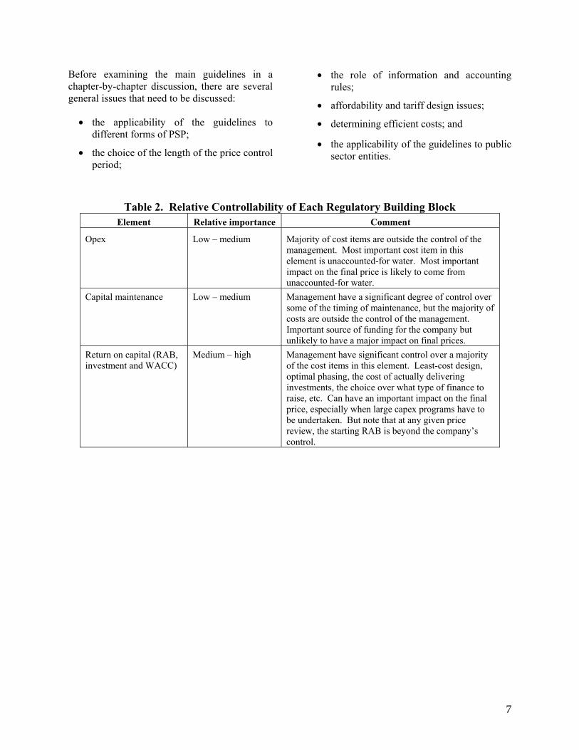
Table 2. Relative Controllability of Each Regulatory Building Block Element Relative importance Comment
Opex Low – medium Majority of cost items are outside the control of the management. Most important cost item in this element is unaccounted-for water. Most important impact on the final price is likely to come from unaccounted-for water.
Capital maintenance Low – medium Management have a significant degree of control over some of the timing of maintenance, but the majority of costs are outside the control of the management. Important source of funding for the company but unlikely to have a major impact on final prices.
Return on capital (RAB, investment and WACC)
Medium – high Management have significant control over a majority of the cost items in this element. Least-cost design, optimal phasing, the cost of actually delivering investments, the choice over what type of finance to raise, etc. Can have an important impact on the final price, especially when large capex programs have to be undertaken. But note that at any given price review, the starting RAB is beyond the company’s control.

8
Figure 1. The Regulatory Building Blocks and Their Corresponding Chapters of the Guidelines
Opex(Chap. 3)
RAB(Chap. 4)
WACC(Chap. 6)
Capex(Chap. 8)
Capitalmaintenance
charge (Chap. 7)
Period-to-periodcorrections
(Various chapters)
Year-to-yearcorrections
(Various chapters)
opex
taxes
WACC x (RAB + workingcapital)
capital maintenance charge
corrections from last period
ALLOWED ANNUALREVENUE
++
++
(Chap. 2)
Use of experts to manage and facilitate the process, and take certain decisions(Chap. 11)
RevenueReq.
Financial viability
Smoothing
Rolling forward the RAB
2.2 Applicability to Different Forms of PSP
The Guidelines make use in many places of material developed in the context of a company that is transferred fully into the private sector through a share sale (the pure privatization approach). In general, regulatory rules that have been developed in this context are the most highly developed. However, the Guidelines are, with some modifications, applicable also to limited-life concessions (see section 4, below).4
4 See Section 2.8 for a discussion of the applicability of the Guidelines to publicly-owned water companies. See also the relevant sections of Groom, Halpern, and Ehrhardt (2006).
Moreover, determining and justifying tariffs on the basis of defined building blocks is equally important if other approaches to PSP were used. Table 3 provides an overview of the building blocks that would be needed under different forms of PSP. Further description of the different forms may be found in the World Bank’s Approaches to Private Participation in Water Services: A Toolkit (2006).

9
Table 3. Different Forms of PSP and the Necessary Building Blocks Form of PSP Opex RAB WACC Capital
maintenance Capex
Service contract ? ? Management contract (?) Lease/affermage ? ? ? Concession ? Privatization
Note: The applicability of using a RAB with a concession depends on the form of concession. In those where a cash-flow neutral position over the life of the concession approach is used—often referred to as the net present value (NPV) approach—no RAB is necessary (although specifying a RAB-type value determined by the NPV approach may be useful). This is discussed further in the Guidelines and in Section 4, below. Areas where “?” have been used in the table are discussed below.
Obviously, the exact need for a building block (or parts of it) will depend on the specifics of the PSP. For example, a concession could use all the same building blocks as a privatization (share sale) or, if an approach that focuses on ensuring cash flows during the life of the concession are met with no terminal value (through an NPV-based approach) is used, then the RAB building block is not needed. Issues relating to the NPV- and RAB-based approaches are discussed in Section 4 of these Explanatory Notes.
In the Guidelines we have tried to highlight some of the differences that arise with concessions rather than full share sales. Further work would be needed to complete the guidelines if they were to be used this way. Other consideration and work would be needed were the guidelines to be considered for one of the other forms of PSP. Further, some of the guidelines may be used but not necessarily in the context of a periodic price review. In that case, further consideration would be needed to ensure that the rules were consistent and applicable without the broader set of supporting rules.
As noted in Table 3, the need for building blocks will depend on the actual details of the forms of PSP being used. It is also not always clear in what instrument the rules for the building blocks should be incorporated. For those forms of PSP where pricing issues are left with the state-
owned entity (even though the private operator may be concerned about the level of revenue being recovered through the pricing regime), there is a risk that any instrument issued by the government or regulator and applying to the publicly-owned entity could be changed in the future (the publicly-owned entity is less likely to complain strongly), thus undermining the credibility of the regulatory rules. PSP might involve the following:
• repeat the regulatory rules in the contract between the publicly-owned entity and the private operator; or
• provide in the main instrument between the state-owned entity and the government or regulator a clause that requires the private operator’s agreement for any change in those specific rules to be allowed.
Transaction advisers and other stakeholders should determine which of the two approaches (or whatever other alternatives are proposed) will work best in the specific circumstances faced.
A brief review of some of the areas where further consideration is needed is provided below.
• Service contracts. Since the payment to the private operator is likely to be based more on inputs delivered, the private company is less concerned about ensuring

10
that tariffs are sufficient to meet all costs. There could, however, be a concern to ensure that at least operating costs are met—or perhaps opex and the most essential capital maintenance; otherwise the entity may not be able to meet the contract costs for the private operator.
• Management contracts. Since the remuneration of the company often depends on cash being available after meeting other operating costs, rules should be established to ensure that the two basic building blocks are included. There can be some uncertainty about capital maintenance since there is an opportunity to shift some of the costs to capex, which is the responsibility of the publicly-owned company or government.
• Lease-affermage. One uncertainty here is linked to the remuneration of existing capital. If this becomes the responsibility of the private operator, through the lease fee, then rules relating to the RAB and WACC (or some other objective rules) need to be established to prevent discretionary changes in the lease fee—and hence in the overall tariff level. In addition, in those cases in which some private capex is envisaged, clear rules are needed for company-specific capex, RAB, and WACC, which could be based on the building blocks in the Guidelines.
• Concession. The only uncertainty in a concession relates to whether a RAB- or an NPV-based approach is used. With NPV, it is not necessary to determine a value for the RAB, as discussed in Section 4, below.
2.3 Length of the Price Control
Finally, how long should the price control period be? Any incentive-based regime requires a multiyear price control period so that the incentives are meaningful. However, the longer the price control period the greater the opportunity for cost differentials to arise—especially in a highly uncertain environment—and for the operator to make significant profits
or losses. This concern has often meant that price control periods in developing and transitional countries are kept on the short side, which reduces the power of some of the incentive mechanisms. On the other hand, the price review process is itself risky, especially in many developing countries, and this could argue in favor of adopting a longer price control period.
Mitigating factors are available to address the concern about substantial profits or losses arising. They include:
• the focus on incentives for controllable costs and making uncontrollable costs pass-through items, although the ability to predict controllable costs may still be limited (especially in the early years of PSP); but one option would be to consider the hard-to-forecast controllable costs as being semi pass-through or full pass-through items;
• the use of clear prudency rules and fixed budgets for items to ensure that incentives exist for managing overruns and unexpected costs;
• the possible use of sharing rules if profits or losses go beyond an acceptable boundary; these rules mean that consumers either benefit from unanticipated gains prior to the end of the price control period or provide additional support to the company if losses are being experienced; and
• an option to include an extraordinary review (ER) if material changes to specified cost items occur or if unanticipated investment arises (this is set out in Chapters [9] and [10]).
While some of these options may make the overall regime a little more complex, they do allow longer price control periods to be used.
What length should a price control period be? The Guidelines have been prepared on the basis of a five-year price control period; this is a period that is generally considered to give a

11
good balance in the trade-off between creating the incentives needed for the company and the goal of not creating too great a risk of excessive gains or losses—a risk which generally increases with the length of the control period.5 Examples of both longer (seven years in Pakistan electricity distribution, and 10 to 20 years for United States electricity and gas distribution) and shorter (three and four years have been used—e.g., four years in electricity transmission in England & Wales) price control periods exist.
One option that could be considered, and is noted in several places in the Guidelines, is for the first one or two price control periods to be short, say three years, before moving to the longer period of five years. While not ideal, this can be a way of addressing poor information issues if the mitigation factors noted above are not felt to be workable in the situation faced or are insufficient to deal with the risk.
2.4 Role of Information and Accounting Rules
Undertaking a price determination, or almost any regulatory decision, requires significant information to be available in a timely and agreed manner—for example, definitions of specific issues should be pre-agreed, etc. In several places in the Guidelines there are references to the need for a business plan. This is one of the primary sources of information for the price determination but not the only one.
Regulatory rules are needed for:
• which information is to be provided;
• the frequency of data provision;
• the definition of any items when they differ from or expand on country-standard accounting definitions;
• the definition of what is covered by the regulatory regime and how common costs, and possibly the whole cost base, for unregulated businesses are to be treated
5 See also Green and Pardina (1999: 45-46) for a discussion of how long the control period should last.
when a regulated company undertakes both regulated and unregulated activities; and
• the physical provision of the data—for example, on a predetermined computer spreadsheet template, in written form, via an Internet portal, etc.
These rules are not provided in the Guidelines but would need to be developed by the transaction advisers as part of the documentation package. If there is a national regulator, it might be even better for the regulator to specify certain requirements as to type and format of information. The regulator or transaction advisors could draw on specific examples or more generic work dealing with these issues.6
Of course, it would not be necessary for the transaction advisers to determine all the accounting rules, etc., rather a clear time bound plan should be incorporated placing responsibility on the regulator and the company to develop the appropriate systems. One issue that clearly needs to be addressed at an early date, however, is the way in which related party transactions are to be handled. Often the ability to sell additional services and/or goods to a WSS services provider is the way in which some of the benefit of ownership is achieved. As such, regulators need to ensure that the prices charged are no greater than those justified by marked based equivalents.
A good reference setting out common issues in the design and implementation of regulatory accounting rules useful for all regulatory
6 As one example, see the Nigerian Electricity Regulatory Commission’s (NERC’s) systematic requirements for information to be submitted by companies proposing power purchase agreements to enable the regulator to assess risk allocation and proposed price in a standardized way (NERC/NOPR/CN04606, December 2006).

12
practitioners is Pardina, Rapti and Groom (2008).7
An issue linked to these accounting concerns is whether a financial model should be incorporated into the bidding process and then used to provide part of the template for information. Bidding models can simplify matters by ensuring a common and standard methodology and basic set of information. This issue should be addressed by the transaction advisers.
Finally, obtaining reliable information on a regular basis about the performance of the company is important as a way to mobilize customer support for the regulatory regime. Systematic rules for information gathering and processing are needed for this purpose, also.
2.5 Affordability and Tariff Design
The Guidelines are concerned with the development of the overall allowed revenue; they do not address the issue of how that revenue should be recovered through the tariff structure.8 While important, the issues relating to design of tariffs (including connection charging and the basis for consumption—e.g., two-part tariffs, increasing block tariffs etc.) require significant knowledge of the local situation and consequently have been left for the transaction advisers to address.
7 Pardina, Martin, Richard Schlirf and Eric Groom (2008) Accounting Infrastructure Regulation – An Introduction, The World Bank, Washington DC. 8 We also do not specify what type of incentive-based regime should be used to recover the required revenue although options for aspects of the different approaches are provided in Chapter 7. Decisions about whether a price-cap, revenue-cap or some form of hybrid should be used will depend on the situation faced by the company and in part the tariff structure (for example, a company will little or no metering will effectively face a revenue-cap even if a price-cap is announced). These issues are discussed in most standard regulatory economics textbooks as well as Alexander & Shugart (2000).
Within this subject is the issue of whether affordability should be a concern for the company or regulator and the ways in which social tariffs can be designed which minimize the perverse incentives while retaining social acceptability. If protection of low income consumers is to be undertaken through the tariff system, then clear revenue-neutral rules need to be established or explicit processes for the state to meet any revenue short-fall that arises because of this requirement.9
Basic tariff issues are addressed in Dinar (2000) while low income consumer issues are addressed in the Word Bank’s New Designs for Water and Sanitation Transactions (2002) and Komives, et al. (2005) and Trémolet and Halpern (2006).
2.6 Determining Efficient Costs
Incentive based regulation requires costs to be forecast for the length of the forthcoming price control period (discussed in Section 2.3). A key element of the incentive is the establishment of targets for the cost components—normally these targets incorporate some expectation about efficiency savings that a well managed company could make.
Benchmarking against the costs of other water companies and other water capex projects, both in the same country and internationally, is an indispensable tool. Experience has shown that it is inadvisable (or advisable only in some limited cases) to conduct rigorous econometric analyses and then mechanically to apply the “efficient cost” figures that emerge without exercising any professional judgment. First, the error due to confounding factors is simply too great. Second, in conditions found in many developing countries, it will not be possible for the company to achieve the ideal efficiency targets right away. A catch-up period will be needed, and professional judgment—influenced significantly by local factors—will be needed to arrive at realistic expectations.
Nevertheless, there is no doubt that consumers can benefit the more information that the 9 See Komives et al. (2005).

13
regulator has about costs in other water systems, the greater the standardization of these costs (e.g., uniform operational definitions of variables), and the greater appropriateness and rigor in the comparative analysis of these costs. However, how to make the best use of benchmarking data—and how best to exercise professional judgment—goes beyond the scope of this work.10
Moreover, in a reduced discretion environment, establishing efficiency targets is far from straightforward. It is not possible to be rigidly prescriptive about how the efficiency targets will be established; rather, a process for determining targets is set out in the Guidelines. This is an area where the role of an external adviser-expert will be vital if credibility is to be established. This role is discussed in Chapter 11.
What is possible, however, is to establish some common sense rules that should be followed. Primarily these revolve around focusing on the key cost items and only establishing binding efficiency targets for controllable cost items. (“Binding” here means that the company will bear the losses (resp. take the gains) if actual costs exceed (resp. are less than) the targets. While it may be possible to establish detailed efficiency targets for some cost items, such as labor costs, given their overall importance in the determination of the final price, it is not
10 See PURC “Survey of Benchmarking Methodologies (March 2006) (describing and assessing different approaches and highlighting the importance of this information for the company itself in its efforts to improve performance); and Torraj Jamasb, Paul Nillesen, and Michael Pollitt, “Strategic Behaviour under Regulatory Benchmarking”, Energy Economics (2004), vol. 26, pp. 825-843 (discussing the various ways that companies can game the particular benchmarking approach adopted by the regulator and setting out lessons to be learned from how regulators have tried to apply benchmarking in setting tariffs). However, care should also be exercised when using benchmarking, see for example “Regulatory Benchmarking: A way ahead or a dead-end?” by Graham Shuttleworth (1999), NERA Energy Regulation Brief no. 3, for a description of some of the pitfalls of using benchmarking in a way that is too mechanical.
worthwhile to expend significant resources determining such targets. It is better to focus on the “big ticket items” like unaccounted-for water, capex, etc., especially in the early years of private sector participation. But it should be noted that it may be more convenient from an administrative and accounting (monitoring) point of view to put several small items in a residual category to be treated as ex ante target—not because they are substantially controllable but because they make up a very small proportion of total opex and so the risks can be easily absorbed by the company.
Finally, it makes no sense to create binding targets for those cost items outside the control of the management of the company. Consequently only those material controllable costs should have binding efficiency targets. Other costs should be treated as cost pass-through items. This does not remove the need to forecast the level of costs for the price control period but it does mean that any deviation from these costs will be passed through to consumers by way of a correction factor. This approach is described in detail in the opex and capex chapters of the Guidelines (Chapters 3 and 8).
2.7 Sanctions Related to Performance Requirements
The two core tasks of the economic regulation of utility companies are tariff setting and the specification and enforcement of performance requirements—what it is that the company is required to achieve. Service standards, in the broad sense of characteristics that customers can perceive, make up most of these requirements. They may also include intermediate outputs that are not perceptible by customers (e.g., underground leakage of water from pipes) but that, for one reason or other may be considered appropriate to be directly targeted by the regulator.
Sanctions of some kind have to be associated with the performance requirements. This is especially important in a regime using ex ante price setting in which the company gains if it can find a way to reduce costs. Without

14
effective sanctions, the easiest way to reduce costs might be to reduce the levels of service.
There are a number of different types of monetary sanctions. Three common types are as follows:
• penalties: the company must pay a specified sum of money to a public authority for each instance of noncompliance with the performance requirements, and for each specified period of time that the noncompliance continues;
• compensation to customers: the payments for certain kinds of non-compliance are made by the company directly to the affected customers;
• an adjustment is made to the revenue requirement for the next control period to reflect divergences of performance from specified target values.11
As an alternative (or more likely, in addition) to direct monetary sanctions, a regime of “deficiency points” could be adopted. In a deficiency point system, a predetermined number of deficiency points accrues for each instance of a failure to comply with a performance requirement. The deficiency points are added up and accumulate over time on, say, an 18-month rolling basis (i.e., the points are ignored if they are over 18 months old).
If the total of deficiency points reaches a certain value at any time, then the regulator is permitted to take a specified action. For example, the different levels might be as follows, with each type of action corresponding to a different (and increasing) level of deficiency points:
11 For an overview of the issues and methods, see the Allen Consulting Group’s report to IPART of March 2001, The Incorporation of Service Quality in the Regulation of Utility Prices: A Discussion Paper. A more general discussion, with a special focus on service provision for the poor, is Bill Baker and Sophie Trémolet, Regulation of Quality of Infrastructure Services in Developing Countries, NERA, May-June 2000.
• warning notice to be sent to the company;
• more intensive monitoring of performance, at the company’s expense;
• a requirement for the company to produce a remedial plan;
• a full technical audit to be carried out by independent technical auditors at the company’s expense;
• notice that the relevant public authority has the right to terminate the contract at any time so long as the total of deficiency points remains above this level.
The purpose of a scheme like this is to provide a meaningful framework for discussions between the company and the regulator about how to deal a problem of chronic poor performance and to provide a reduced discretion rule for when the company’s performance is so deficient that the relevant public authority has the right to terminate the contract.
Although the question of how to design and implement positive or negative sanctions is an essential function of any regulatory regime, the Guidelines and the Explanatory Notes to the Guidelines do not consider this topic.
2.8 Role of the Guidelines With Respect to Public Sector Entities
The Guidelines have been prepared on the basis of regulating a private sector entity that responds to financial incentives. Can they be applied to public sector entities? Certainly the idea of determining allowed or required revenue on the basis of well-defined building blocks is a valuable approach that can be applied to tariff setting for any publicly-owned water company. It can serve to operationalize a cost-recovery policy, provide increased transparency with respect to the performance of the company, and provide a framework to increase the effectiveness of performance agreements.12
12 See, in general, the relevant section of Groom, Halpern, and Ehrhardt (2006).

15
In principle, the incentive properties of the approach set out in the Guidelines could be applied to publicly-owned companies, too, but only if certain conditions are met such that the public sector company acts to a large extent as though it were a private entity—that way it should respond the same way to incentives. The Chilean water companies before privatization faced an environment of corporate governance and commercialization that enabled them to respond to regulation as though they were private companies. The conditions in which applying regulatory rules as though a public sector entity were a private one are often not met. Consequently, applying the Guidelines in their entirety is unlikely to provide the desired outcome and, if the attempt fails, could actually destroy
regulatory credibility rather than enhance it. However, some of the elements of the Guidelines could still be used and some of the principles followed. But care should be taken in deciding what is needed. Possibly the most important aspects that can be applied are those relating to information definition, collection and analysis. In general, much work remains to be done to develop a sound and comprehensive framework for regulating publicly-owned water companies (using “regulating” in a very broad sense).13
13 For some ideas, see, for example, Maria Vagliasindi (2008), Governance for State Owned Enterprises, World Bank Policy Research Working Paper 4542; Anton Eberhard (2007), Is it possible ton regulate state-owned utilities effectively?, presentation at the PURC/World Bank International Training Program on Utility Regulation and Strategy; Tim Irwin and Chiaki Yamamoto, Some Options for Improving the Governance of State-Owned Electricity Utilities, Energy and Mining Sector Board Discussion Paper No. 11, World Bank, February 2004 (broadly applicable to the water sector also); Aldo Baietti, William Kingdom and Meike van Ginneken, Characteristics of Well-Performing Public Water Utilities, Water Supply & Sanitation Working Note No. 9, World Bank, May 2006. For a historical background and reflections on ways forward, see Gómez-Ibáñez (2007).

16
3.
RULES AND DISCRETION
3.1 Different Kinds of Rules The idea that there are trade-offs in using, on the one hand, sharp or precise rules and, on the other, broader principles has been discussed at length in the legal and law and economics literature for many years.14 For example, an area of application close to the present topic is competition law. In the United States, the Supreme Court in the first half of the twentieth century made a distinction between “per se rules” and the “rule of reason.” Applying the rule of reason, a court would have to examine all the facts relevant to the business and all the effects, actual or probable—all in the light of the broad objectives to be served. In contrast, a per se rule describes specific practices that are conclusively presumed to be illegal, without the need for an elaborate inquiry. Principles necessarily involve high discretion in decision making. Principles tend to predominate in primary legislation relating to the economic regulation of utilities.15 For example, one telltale sign of a principle is the prescription to “balance” various interests, all things considered. Broad rules can also be preferred by the agency that writes the secondary legislation if that agency (e.g., a regulator) will be responsible for implementing the rules. There is often a natural bureaucratic tendency not to want to tie one’s hands, although this will depend in part on the agency’s expectation of how the appeals body is likely to respond.
14 The terms used to describe the two polar types, which in fact exist on a continuum, are varied. The law and economics literature often refers to them as “rules” versus “standards,” but the present report prefers to use “rules” in a more general way to encompass all types. We will generally speak of precise or sharp rules versus principles. 15 But not in some countries, for instance, Chile.
3.2 Advantages and Disadvantages of
Low-discretion Rules Scholars and practitioners have noted the costs and benefits on both sides. The main advantages of sharp rules that are often discussed in the literature are as follow. Sharp rules:
• provide greater certainty and predictability—they aid in creating credible commitment;
• give more consistent treatment and greater fairness;
• help reduce the scope for arbitrariness and bias;
• provide more constraints on political influence;
• are to be preferred if the decision making body does not exhibit high competence (despite the possible presence of highly competent individuals within it) or is in a start-up stage and in the process of building up its capacity; and
• save time and cost when each specific case is considered—i.e., the decision maker does not have to go back and work through basic principles for each decision, and the information requirements are greatly reduced.
The main disadvantages of sharp rules are as follows (in some cases expressed as the advantages of principles):
• Precise rules may give the wrong decisions in some cases, especially if the circumstances diverge greatly from what was contemplated when the Guidelines were formulated. (This is the basis for one of the main criticisms, in some sectors, of long-term contracts as a means of

17
regulation: conditions are likely to change too much over the duration of the contract.)
• If the decision maker is competent and unbiased, principles will result in better decisions since they go back to basic policy objectives and considerations.
• The initial set-up cost of a system of sharp rules is high; all the rules have to be carefully thought through and developed in detail.
• Using principles and discretion can allow the regulator to stay one step ahead of the company; the company will probably find all the loopholes and will figure out how to manipulate the rules to its best advantage.
• If the set of precise rules becomes too complex in an attempt to cover every contingency no matter how minor, ambiguities can increase, allowing the rules to be manipulated by the regulator to give the desired result—but in way that is not transparently related to underlying objectives. In other words (given bounded rationality), increasing the complexity of sharp rules can actually increase the possibilities for discretionary decision making.
A balance is needed—one that is optimal for a specific context. The Guidelines take the view that, with respect to the regulatory rules used for water and wastewater utilities in many developing countries, moving more towards the low-discretion end of the spectrum will bring benefits that more than offset the additional costs. Users will have to decide if this holds true in their own circumstances.

18
4. EQUIVALENCE OF RAB AND NPV APPROACHES The Guidelines have been written using the conventional regulatory accounting approach—making use of the RAB, regulatory depreciation, and so on. In concession arrangements, tariffs are often reset in a different way, using a long-term cash flow model with the NPV as a criterion (we will refer to this here as the “NPV approach”). For an indefinite-duration arrangement, as with a full privatization, the RAB method is certainly to be preferred. With regard to a limited-life concession, however, there are advantages and disadvantages to each approach. One advantage of the NPV approach is that, when carried out in the early years of the PSP arrangement, it makes tariff-smoothing over any desired period easier to achieve; this may be important in systems that are starting out with a large backlog of capex to implement. On the other hand, the NPV approach, by itself, provides no constraints at all on the time-path of cost recovery; this is far from being a reduced discretion method. But additional rules could be added to provide the needed constraints, especially related to financeability. Also, additional rules would need to be developed to deal with the question of whether full cost recovery of capex must take place over the term of the concession or whether there will be a residual value—equivalent to a closing RAB—at the end of the concession (cf. §7.4).
Another possible drawback of the RAB method is that some regulators feel uncomfortable with negative RABs. Given that up-front entry payments are generally frowned on in water
concessions,16 where there is often a concern that any major increase in tariffs will be politically and socially unacceptable, if a concession is regulated using the RAB approach, the RAB might fall below zero at some point during the first few years. (Of course, other kinds of accounting adjustments could be used to deal with the issue while staying within the classic RAB framework—changing the presentation but not the substance.)
Some readers may initially assume that the Guidelines are inapplicable to the NPV approach—and by extension to most limited-life concessions. This is not so. Every part of the Guidelines that deals with how tariffs are set using the RAB, regulatory depreciation, etc., could be translated into an equivalent set of rules within the framework of the NPV approach. We will not demonstrate this statement in any rigorous way in the Explanatory Notes to the Guidelines;17 instead we will illustrate it with an example.
The three tables below show the adjustments that would need to be made under the RAB and the NPV approaches to take into account a discrepancy between target capex and actual capex using one variant of the ex ante ex post method (as set out in §8.4.3, Variant A).
The calculations are simplified; the tables show only the values needed to illustrate the point being made—e.g., opex is not included. All cash flows are assumed to occur at the end of the year. The entire analysis is done in real terms. The discount rate used is 11 percent. It is assumed for simplicity throughout the tables that
16 For example, entry fees in water concessions in France have been illegal since 1995. 17 See Green and Pardina (1999), Chap. 5, for further discussion.

19
we know the actual costs incurred during year five at the end of that year.
Table 4 shows the important assumptions about capex during one five-year control period. The cumulative actual capex over the period is less than the cumulative ex ante—estimated capex by 40, even though in two years the actual is greater than the ex ante estimated (lines 1 and 2). If no adjustment were made ex post, the company would receive a gain of 31 in present set out in §8.4.3, Variant A. For this RAB method, we stipulate depreciation on existing value terms by reducing actual capex below the values used to set tariffs during the control period (lines 3 and 4).
Table 5 illustrates the RAB-based method that is assets and an opening RAB (line 5, year 1; and line 6)—the values do not matter for what follows. Depreciation of new assets, based on estimated capex, is calculated assuming a 30-year asset life and straight-line depreciation (see total depreciation in line 5, years 2 to 5).
Table 4. RAB-based and NPV-based Approaches/Assumptions
Sums 1 2 3 4 5 1 Estimated capex 500 100 100 100 100 100 2 Actual capex 460 80 120 70 80 110
3 Present value (PV), estimated 369.6 4 PV, actual 338.6
Table 5. RAB-based Approach
1 2 3 4 5
5 Depreciation 20.0 23.3 26.7 30.0 33.3 6 Starting RAB (end year 0) 100
Based on estimates (ex ante)
7 RAB (end of year) 180 257 330 400 467 8 Return on RAB 11 20 28 36 44 9 Revenue requirement 31 43 55 66 77
10 After adding terminal RAB 31 43 55 66 544 11 NPV 469.6 12 After subtracting starting RAB 369.6
“Classic” adjustment
13 RAB (ex ante) 180 257 330 400 467 14 Correction to ending RAB -40 15 Corrected RAB 180 257 330 400 427 16 Return on RAB 11 20 28 36 44 17 Revenue requirement 31 43 55 66 77 18 After adding terminal RAB 31 43 55 66 504 19 NPV 445.9 20 After subtracting starting RAB 345.9

20
Line 9 shows the annual revenue requirements based on the RAB method. The revenue requirement is equal to the sum of depreciation and the return on the RAB (at 11 percent per year). If we take the NPV including the ending RAB and subtracting the starting RAB (line 12), we see that the result is the same as just finding the NPV of the estimated capex—the result in line 3.
Lines 13 to 20 show the classic RAB adjustment method carried out after learning the actual capex values: we deduct the sum of the differences between estimated and actual capex from the closing RAB (which is the same as the opening RAB of the next control period). We do not need to show the revenue requirement in the next control period because the impact of the reduced RAB in the next period is entirely accounted for by the reduction of the RAB at the start of that period.
The NPV of the adjusted revenue requirement for the first period (line 20) is lower than before (line 12) because we are making a correction downwards to reflect actual capex.18
The NPV-based approach is shown in Table 6 using two different calculations. The most straightforward calculation is shown in lines 21 to 24. This begins with the ex ante—estimated values and makes a one-shot correction in the last year of the control period to reflect actual capex (line 22). New forecast and target values would be used for year 6 and onwards. (An adjustment like this is not normally done in resetting tariffs for concessions: usually the past capex values in the model are either kept at the previously estimated values or they are entirely replaced by actual capex values.) The NPV of the cash flows (line 24) is the same as that determined
18 Note that the value in line 20 is invariant to the pattern of the discrepancies between estimated and actual capex over the five-year control period (e.g., the value in line 20 would not change if the entire difference of 40 occurred in year 1 (see line 2). All that matters in the classic adjustment method is the total difference over the five years of the control period.
using the RAB approach, showing their equivalence. There are other equivalent ways that one could proceed using the NPV approach. One alternative calculation is shown in lines 25 to 36. This starts instead from the actual capex figures (line 34), which would replace the previous target figures in the model at the next price review.
The adjustment this time is determined by calculating the “interest” (carrying cost or benefit—here done using the WACC of 11 percent) on the difference between estimated and actual in each year (line 28) and then applying this value to each of the remaining years of the control period (lines 29 to 32). For example, in year 1, the company under-spent the capex target by 20. So, in addition to being allowed to recover its actual costs, it is allowed to receive a return on the amount of under-spend in each of the remaining years of the control period (line 29). This way of looking at the correction brings out clearly the incentive that the company has to reduce its expenditures below the ex ante values; it also makes it readily apparent that the incentive is greater when the under-spend occurs early on in the control period because then the return on the discrepancy applies over a greater number of years (e.g., line 29).
Actual capex is then adjusted by the sum of these gains or losses (line 35) (these adjustments would be entered into in the financial model used in the tariff determination). The NPV (line 36) is the same as using the simple calculation.
Of course, the simple calculation is the one that should be used in actual practice. The alternative calculation has been shown here to highlight the intuition behind the adjustment, which may not be readily apparent by looking simply at the single adjustment in year 5 (line 22).
All the other provisions of the guidelines (including all variants) relating to the revenue requirement and how it is set and adjusted could be re-expressed within the NPV framework. It

21
is interesting to note that most concession agreements in the water sector do not develop these rules in any detail—which leaves them to
be worked out implicitly and informally by the parties during periodic renegotiations.
Table 6. NPV-based Approach 1 2 3 4 5
Simple NPV calculation 21 Estimated capex 100 100 100 100 100 22 Correction based on actual values -40 23 Adjusted cash flows 100 100 100 100 60 24 NPV 345.9
Alternative NPV calculation
25 Estimated capex 100.0 100.0 100.0 100.0 100.0 26 Actual capex 80.0 120.0 70.0 80.0 110.0 27 Difference 20.0 -20.0 30.0 20.0 -10.0 28 Annual interest (carrying charge) 2.2 -2.2 3.3 2.2 -1.1
29 Re year 1 2.2 2.2 2.2 2.2 30 Re year 2 -2.2 -2.2 -2.2 31 Re year 3 3.3 3.3 32 Re year 4 2.2 33 Sum 2.2 0.0 3.3 5.5
34 Actual capex 80.0 120.0 70.0 80.0 110.0 35 Adjusted cash flows 80.0 122.2 70.0 83.3 115.5 36 NPV 345.9

22
5.
EXPLANATORY NOTES TO THE GUIDELINES, CHAPTER-BY-CHAPTER N.B. For ease of reference, subsection numbers (beginning with “CH”) in this section are keyed to the corresponding chapter numbers in the Guidelines; § references are for specific sub-sections of the Guidelines.
5.1 Introduction: The Building Blocks The Guidelines broadly follow the building block approach illustrated in Figure 1. In the periodic review, the revenue requirement for the next control period is built up by adding the values shown on the right side of Figure 1. The different building blocks are described in the sections below.
A brief word should be said about the “year-to-year” and “period-to-period” corrections (lower left boxes in Figure 1). Year-to-year corrections apply within one control period. For example, if a certain cost item is to be treated as a pass through, then any discrepancy between forecast and actual costs in year t will be treated as a correction to the allowed revenue for year t + 1. Period-to-period corrections refer to corrections made to the revenue requirement for the forthcoming control period based on values in the previous control period; these could be the same in substance as the year-to-year corrections except that they spill over into the next control period and are taken into account over the entire control period by adjusting the overall revenue requirement for the next control period.
It should be noted that Figure 1 shows just the core of the process and does not go further to show the factors that influence the building blocks. For example, opex and capex must be determined with reference to target service standard, including network expansion targets. These are not shown in Figure 1.
CH1. General Provisions
Chapter 1 of the Guidelines sets out some definitions, notation for the formulas used in the Guidelines, rules for interpretation, and conventions used in discounting cash flows. This chapter would need to be developed much further in the actual rules—this is work for system-specific advisors.
CH2. Allowed Annual Revenue
Determining the Allowed Annual Revenue at the Price Review
The first part of Chapter 2 describes how the values to be determined in the following chapters are combined to yield the allowed annual revenue for each year of the forthcoming control period. (The “control period” is the period between two successive periodic reviews.) Since the Guidelines do not address the issue of tariff structure, in presenting the calculations for the allowed annual revenue we have assumed the simplest of tariff structures: a single volumetric charge (price per cubic meter). Modifications would have to be made in certain sections of this chapter if a more complicated tariff structure were to be adopted.
The basic steps are as follow:
• Build the revenue requirement for each year of the forthcoming control period. This is done by taking the sum of the following items for each year, based on targets or forecasts developed in accordance with the following chapters of the Guidelines:
opex; taxes; capital maintenance charge;

23
(RAB + working capital) x allowed rate of return;
any corrections to be applied from previous control periods.
• Determine the present value (as of the start of the new control period) of the revenue requirement.
• Based on demand forecasts, determine a smoothed tariff profile over the control period that yields the same present value of revenue. This is done to help avoid fluctuations of the tariff over the control period, which might occur if the annual revenue requirements were translated directly into annual allowed revenue. The smoothing must be done, however, in an NPV-neutral manner (i.e., the NPV of the allowed revenue remains the same even if the time pattern changes). The annual revenue figures that emerge from this step constitute the allowed annual revenue. One constraint included in the Guidelines is that the allowed revenue in any year must at least equal the estimated opex for that year: i.e., one can smooth tariffs by shifting return on or of capital, but not by permitting revenue in any year to be so low that it does not even cover opex (i.e., the company should not have to finance opex).19 Another important constraint (related to financial viability—see below) is that, to the degree that this is possible, allowed revenue must permit the company to meet lender’s cover ratio covenants.
Smoothing is also possible, and in some cases advisable, between control periods as well as within a control period. For example, in some circumstances it could be critical for financial viability related to debt service payments or if large multiyear investment projects straddling more than one control period are envisaged. Guidelines for handling this kind of adjustment are not included in Chapter 2.
19 This does not imply, however, that the tariff for each customer must necessarily cover the opex attributable to that customer. The discussion in this section is about allowed revenue or average tariffs—not about tariff structure.
Correction for Changes in the Volume of Water Sold
The determination of allowed revenue is made during the price review. This does not mean that (even disregarding inflation adjustments) allowed revenue in each year of the forthcoming control period will remain as it has been determined during the price review. Chapters 3 and 8 deal with various adjustments relating to pass-through cost items. But there are possible adjustments on the revenue side, too. The most important is a correction for changes in the volume of water sold.
Concession arrangements in which the operator’s remuneration is a price per cubic meter of water sold often face difficulties in the face of changing demand for water. Some of the operator’s costs vary with volume of water—the main items being chemicals for water (and wastewater) treatment, electricity for pumping, and in some cases the price of raw water paid to an external supplier or a water resource fee paid on a volumetric basis to an administrative authority. But a large part of the operator’s costs are fixed. Changes in the volume of water sold can therefore lead to large swings in net cash flow—sometimes pushing the operator into financial distress.
In a service system with many unconnected households, as is often found in developing countries, in some circumstances a volumetric price can give a strong incentive to the operator to make new connections.20 But if the concessionaire’s revenue requirement over the price control period has been set based on the expected number of connections that the concessionaire can implement and a forecast volume of water sold to each connection, then
20 This depends, among other things, on the tariff structure. There may be a low “lifeline” tariff rate for the first block of consumption (e.g., 8 to 15 cubic meters/month) and many customers in the target geographical area may not be expected to consume much more than that. Also, the unserved areas may have higher costs per connection. The result of these conditions may be that the operator would incur a net loss by extending connections to that area, even if its revenue is increased.

24
failure to meet these two targets can lead to large losses. An alternative would be to set the target number of connections at a highly pessimistic level, but it might be difficult politically to justify such an ex ante decision to give the concessionaire an expected windfall.
Another important factor that leads to inaccurate sales volume estimates is the decrease in per capita consumption that usually occurs when customer meters are introduced and, at the same time, tariffs are increased. It is difficult to predict with any confidence how much of a decrease will occur in a particular country and service system.
For these reasons, concession contracts often contain provisions that allow for an extraordinary price adjustment if the volume of water sold changes substantially from one year to the next or (a better approach) is substantially different from the target volume on which the present price for that year was based.
There are advantages to using a mechanism that would work automatically during a price control period. The mechanism has to sacrifice some precision, but the benefit is to reduce discretion and hence the possibility of long wrangling and disputes—and to cut the costs of the review process.
Chapter 2 of the Guidelines sets out a simple method that uses the breakdown of opex from Chapter 3 so that allowed revenue in each year is corrected ex post based on actual volume figures so that the operator in effect receives (a) the target volumetric cost per cubic meter of water sold multiplied by the actual quantity of water sold in that year; plus (b) the target fixed portion of allowed revenue (fixed opex and return of, and on, capital). In the terms often used by conventional regulators, the volumetric component is treated as a price cap and the fixed component is treated here as a revenue cap; the combined arrangement is sometimes referred to as a hybrid price-revenue cap.21
21 For further discussion of these issues, see Alexander and Shugart (2000).
The problem with a binary method (full correction or no correction, with nothing in between) is that it does not give any incentive for the operator to increase the volume of water sold—an objective that is often important in a developing-country context—since in the full-correction regime the operator does not keep any of the additional net cash flow gained by increasing sales. There are three general ways to remedy this failing. One way would to disaggregate the factors contributing to changes in volume, separating changes in the number of connections from changes in water sold per connection, and then correcting only for changes in water sold per connection, in the assumption that this is something substantially outside the control of the operator (or perhaps something that the operator should be trying to decrease in the interests of water conservation). Chapter 2 does not set out this method, but it is not difficult to develop the needed rules and formulas.
Following the general principles in the Guidelines, if it is possible to disaggregate controllable and uncontrollable components, it would be better to proceed in this way. But one drawback is that the correction formula in that case could become complicated and its workings could become obscure. So a second method would be to apply a partial correction of some sort for changes in the volume of water. This would give the operator some incentive to increase water sold. This is the simple approach taken in Chapter 2.
A third way, and perhaps the best way, would be to apply a full correction for changes in the volume of water but then introduce a separate incentive specifically linked to the number of new connections made by the operator as in output-based aid.22
Financial Viability
Chapter 2 also addresses the problem of how a set of reduced-discretion regulatory rules should deal with lenders’ cash flow requirements that might push the regulated company into
22 For output-based aid, see: www.gpoba.org.

25
insolvency.23 A particular issue that arises in a regulatory context is that many regulators (and these guidelines) use a real WACC and deal with inflation by indexing the RAB and depreciation; whereas lenders generally deal with expected inflation by using nominal interest rates,24 which front-loads the impact compared with the revenue requirement set by a real-WACC regulator. For example, looking only at debt, suppose that the real interest rate is 5 percent and expected (and actual) inflation is 6 percent. Even though the NPV will be the same, there will be a mismatch of cash flows if the regulator allows revenue based on an interest rate of 5 percent but increases the base by 6 percent a year, whereas the lender requires interest payments of about 11 percent based on a fixed nominal loan principal amount. This problem can be mitigated by the company using a lower gearing ratio, but companies may view this as a suboptimal solution.
The most important way to assure financial viability is to set out clear rules before the involvement of the private sector and hence before debt agreements are entered into that describe the way that the regulator will set tariffs so that lenders will be reassured that the regulator will not set tariffs later in a way that would jeopardize the timely payment of debt service (provided the company is reasonably efficient). Making ex post adjustments to address financial viability issues in an ad hoc manner draws the regulator into the difficult and confusing task of trying to determine the degree to which impending financial distress is due to unreasonable conduct on the part of the company or unreasonable requirements by its financiers—or on the part of the regulator. The philosophy of the Guidelines, in general, is to set the rules of the game before any private
23 A useful discussion of this issue is found in the discussion paper Financing Networks, issued jointly by Ofwat and Ofgem in February 2006, along with a Summary of Reponses in August 2006. The issue has taken on a particular importance in the United Kingdom because of the increasing gearing of some of the regulated companies. 24 Index-linked loans or bonds are not common in corporate or project finance.
involvement, get buy-in from potential financiers, and then not intervene later.
The problems of credible commitment and hold-up still arise. If a lender and company, knowing the rules in advance, still create conditions in which reasonable, rule-abiding tariff-setting by the regulator can threaten to drive the company into insolvency, will the regulator allow the company to go bankrupt (or call the lender’s bluff, thus forcing a restructuring of the financing) or will the regulator cave in and increase tariffs to take the company out of danger?
Because of this problem, which might be accentuated in a developing country context, the Guidelines suggest an approach in which the regulator specifies ex ante a maximum gearing ratio for the company. This ensures that there will be a sufficient equity cushion to soften the impact to lenders of rule-conforming tariff adjustments. This approach might be considered intrusive, and in mature regulatory regimes it might not be necessary, but the benefits in the early years of a new regulatory system in many developing and transition countries would probably outweigh the costs.
The maximum gearing ratio would be based formulaically on the allowed rate of return, the expected cost of debt, and the minimum interest cover ratio considered acceptable (§2.5.1)—which would in turn be based on the expected riskiness of cash flows—and should be discussed with potential financiers in advance.
The Guidelines contain two important qualifications to the use of the maximum gearing ratio. First, this approach would only apply to the traditional corporate finance model (where a loan is made considering the company as a whole), not to other models of the “structured-finance” variety—e.g., a model in which cash flows relating just to the asset base are separated out and isolated from other cash flows and are used to pay debt service. Second, a higher gearing ratio would be acceptable in certain circumstances during early phases in which large backlog investment programs are being financed, provided that no distributions of any kind are made to shareholders until the gearing

26
drops below a specified value (cash lock up provision). It is often easier to convince equity investors to refrain from taking dividends out during an initial period (even though they do not like it) than to put in more equity at the start—and in certain circumstances this will be acceptable to the lenders.
Apart from these specific provisions, Chapter 2 emphasizes the use of two special financial ratios as key indicators of the financing capabilities of regulated water companies: an adjusted interest cover ratio (with depreciation deducted from the numerator) and a special measure of gearing, the debt-to-RAB value (where debt here means net debt—see definition of net debt in Chapter 1 of the Guidelines). The Guidelines make use of these ratios, which are shown to be related to each other, and focuses primarily on the latter, the debt-to-RAB, and value as the measure of financeability.
There is no need for regulators to set explicit targets for half a dozen different indicators, although a good financial model should be able to calculate the standard range of financial indicators and all should be considered as a check on financeability. In the approach adopted here, however, these are secondary to the debt-to-RAB measure.
When setting the appropriate value for debt-to-RAB, care will need to be taken. Many of the financial ratios and quantitative rules of thumb typically used by lenders and rating agencies to assess the creditworthiness or financial health of commercial companies are derived from analyzing companies that are not regulated utilities. The particular features of regulated utilities need to be borne in mind and the ratios and values used should be adapted to the context. Owing to the greater certainty of revenues, regulated utilities might be able to obtain an investment-grade credit rating with certain financial indicators appearing worse than what a nonutility company would need. It is important for regulators to maintain a dialogue about these issues with major lenders and rating agencies.
CH3. Operating and Maintenance Expenditures (Opex)
Different Components of Opex
Chapter 3 of the Guidelines describes how the revenue requirement relating to operating and maintenance expenditures (opex) is to be set during the periodic review and then adjusted during the control period. Opex is less complicated than capex because cost recovery is not spread out over time, but rules still need to be specified.
Opex is broken down into three components: fixed cost (i.e., not significantly related to volume or customer number); costs related to the volume of water or wastewater; and (if considered appropriate) costs related to the number of customers. Breaking opex down in this way is useful for purposes of estimating costs (including assumptions about expected efficiency gains) and can then used to adjust opex during the control period in response to the respective drivers. For the latter purpose, it is also useful to break opex down into components that are largely controllable by the company and those that are substantially outside the company’s control—and also to identify mixed components.
Estimating Future Opex and Setting Targets
The allowances for opex for the forthcoming control period would be based on information provided in the company’s business plan, as a starting point. The guidelines do not set out methods to be used to estimate reasonably efficient opex—the target values; but the actual regulatory rules adopted would probably want to go into somewhat more detail.
Estimates would normally be made using some combination of past company costs, costs of other companies in the country, engineers’ estimates, and international benchmarks. The particular mix will depend on the particular circumstances—especially, the adequacy of good cost accounting data and the existence of reliable comparators in the country. Also, the better and more representative the information is, the more one can make use of a top-down approach: looking at total opex, adjusted to

27
reflect the basic characteristics of the particular service system (e.g., number of customers, density of customers), and then adjusting for special factors. This is the approach used for instance by Ofwat. Using data from comparators is not a simple matter, however, and requires good professional judgment (see Figure 2).
When benchmarks based on other companies are used, attention should especially be paid to opex-capex tradeoffs: a comparator company may have been able to achieve very low opex by shifting the mix of costs more to capex. If the regulated company is not using the same mix, it would be misleading to think that “efficient opex” for it is the same as for that comparator.25
25 See Cubbin (2004).
Figure 2. Aspects to Consider in Interpreting Opex Data from Comparators
ACTIVITIESAbstraction & treatment
Water distributionSewage collection
Sewage treatment (bytype)
Billing and collectionEtc.
MAIN DRIVERSAsset characteristicsNumber of customers
VolumesNon-revenue water
Average pumping headSize of drainage area
Etc.
ECONOMIES OF SCALEAND DENSITY
TRADEOFFS BETWEENOPEX AND CAPEX
Estimate of reasonablyefficient opex

28
Where conditions for a specific company are expected to be considerably different from the past and few if any reliable comparators are available—conditions likely to be encountered at first in many developing countries—it may be necessary to rely more on a bottom-up approach, building up opex from its basic components.
Glide paths—gradual decreases in a cost item over the control period—should be included where they are based on realistic assumptions about what a reasonable operator should be able to accomplish in the circumstances, based on the same sources of information mentioned above. In a full set of limited-discretion rules, it might be advisable to include certain requirements or constraints relating to the profile of opex glide paths—e.g., to reassure the company that unreasonable increases in efficiency will not be required. For example, the regulator should be obliged to provide justification for glide paths used; it should not simply be assumed that a particular opex item should decrease by a certain arbitrary fixed percentage per year—e.g., 3 percent (without justification). Also, it might be good to specify that the target level of an opex item in the first year of the next control period cannot decrease below the average level of the past few years of the immediately preceding control period by more than the new glide path rate (or the glide path rate times a specified factor), unless there is special justification—i.e., the regulator cannot baldly ignore the actual past costs of the company.
Ex ante and Cost Pass-through Methods of Treating Opex
The Guidelines set out two main ways that items of opex can be treated—and the actual regulatory rules would list the different items that are to be treated in the two ways.
• Ex ante method. This is “price cap” style, in that the estimated cost is fixed, year-by-year, and the company takes any gains or losses based on its actual expenditures (§3.2.2(b)). This provides strong incentives for the company to control costs. Variants on the basic ex ante
method can be used. For example, if an appropriate specific price index exists (not based on the actual prices that the firm obtains), this can be used for the price component and the quantity component can be fixed ex ante.
• Cost pass through. The best estimates are made and used for the revenue requirement, but then a positive or negative correction is made to allowed revenue in every year t + 1 to compensate for overspend or under-spend, respectively, in year t (§3.2.3(b)). Financial carrying charges are added in making the correction (§3.7). If actual opex exceeds the estimated expenditure by more than 10 percent, then the over-spend (§3.2.3(c)) will be assessed for its prudency.
Hybrid approaches are noted below.
Considerations in Deciding Which Approach to Use
There are a number of considerations that should go into the decision to classify an opex item as subject to the ex ante or pass through method. Any of the following conditions tends to favor the use of the ex ante method. (The conditions are expressed as if the default method is cost pass through and a decision is being made as to whether some cost items should be treated by the ex ante method. Alternatively, the conditions could have been expressed starting from the ex ante method as the default approach.)
• The particular cost item is largely controllable by the operator. Transferring the risk to the operator has no incentive effect if the cost is beyond the operator’s control. All this does is add risk to the operator’s cash flow. (But there may be other reasons for having the operator bear the risk, especially if it is small.)
• The operator’s efforts would have a substantial impact on total costs. This is a de minimis consideration. The cost item

29
may be controllable, but the degree to which the cost can be reduced or increased by the operator’s efforts may be very small.
• Good information is available to be able to estimate future costs accurately (high predictability). If the information is very poor, the cause is different but the result is the same as if the cost is largely uncontrollable: treating the item on an ex ante basis adds a great deal of risk—and risk of a particularly undesirable kind. Poor baseline information when making estimates during the price review will tend to produce over- or under-estimates that persist during the control period (positive serial correlation of errors) rather than a series of independent random errors. This means that the cash flow impact (positive or negative) is likely to increase over time.
• Costs are clearly separable and so there are low opportunities for gaming by the operator. If costs can easily be reclassified from the ex ante category to a cost pass-through category through creative accounting, or if pass-through costs can easily be substituted, trying to impose the ex ante method for that item may not be worth the effort.
In addition, since it runs for a longer period without reference to actual costs, the ex ante method has advantages if the company has an inadequate cost accounting system in place (e.g., in the early years before a good system is set up and fully operational) and the actual costs expended are difficult to verify and audit. Also, the ex ante method gives the company an incentive, indirectly, to reveal information about efficient costs, which can be useful to the regulator in setting prices at the next review. Finally, it is important to look at the entire system and bear in mind the possibilities of perverse incentives. For example, if preventive maintenance (as an opex item) is handled using the ex ante approach but capital maintenance is treated more as a cost pass-through, the operator might have an incentive to spend less than the optimal amount on preventive maintenance,
preferring to let assets deteriorate at a faster pace.
Methods Suited for the Initial Phase When Information is Very Poor
The Guidelines give a variant set of guidelines that could be included to cover the first control period (if five years) if baseline information is very poor—e.g., when a PSP arrangement takes over from a very poorly run publicly-owned company, or one that was not in a corporate form but was formerly a service unit of a ministry, where not all costs for the water services were accounted for separately. Several years may be needed to get the data needed to have a good baseline of costs. The two modified mechanisms are as follows:
• Partial pass through (§3.3.2). This could be used for a cost item that is in principle substantially controllable by the operator but there is very poor information about existing costs or about what reasonable costs should be in the future. It could also be used for cost items that contain mixed controllable and uncontrollable components and poor accounting or reporting prevent better disaggregation. The item is treated mostly as a cost pass- through, but a small incentive component is included to encourage the company to try to reduce costs—which will help indicate what reasonable costs are at the next price review.
• True up (§3.3.3). A cost item treated in this way is treated as a pass-through or a partial pass-through until the company puts an adequate information system in place (to be verified by an independent auditor). At that point, data is collected for one full year and a baseline cost is set; the mechanism then shifts to ex ante (i.e., price cap style) for the rest of that control period and in all future control periods. If this method is adopted for some cost items, sanctions of some kind should also be built in to ensure that the operator takes the required steps to establish an acceptable information measuring and recording system in a timely manner.

30
Detailed Treatment of the Volumetric Component of Variable Opex
The Guidelines also set out, as an example, a way that the volumetric component of opex could be handled (§3.5). (The unit cost (per cubic meter of billed water) and the quantity of water are dealt with separately since the factors to take into consideration may argue for different treatments. In general, the quantity component would be treated more as a pass through.) With one exception, there is no reason why this cannot be handled on an pure ex ante basis after any initial short phase of poor information. During the price review, estimates would be made, year by year, incorporating reasonable improvements in efficiency, if appropriate, for the following variables:
• cost of electricity per cubic meter of water and wastewater pumped;
• cost of chemicals per cubic meter of water and wastewater treated;
• cost of raw water per cubic meter; • coefficients for each of the three items
above to convert the costs into costs per cubic meter of billed water or wastewater (and as with the three unit costs, the stipulated coefficients might change from year to year); and
• estimated reasonable collection efficiency.
The stipulated ex ante cost per cubic meter of billed water or wastewater can then be determined for each year of the control period.
Targets for nonrevenue water (which might change year by year according to a glide path) are what determine the coefficients used to convert the basic unit costs into costs per cubic meter billed. For example, if the stipulated cost of electricity is c per cubic meter of water pumped and a target of 80 percent is set for the percentage of water pumped that will end up as water billed, then the company will be allowed to charge c/0.8 per cubic meter billed (or targeted to be billed) for electricity. If the company decreases non-revenue water below 20 percent, then it can keep the gain from the electricity component because the coefficient of 0.8 is set ex ante.
The only item not handled on an ex ante basis is the price of raw water, if purchased or if based on a water resource charge set administratively. The price is handled on a full pass through basis, but not the cost per cubic meter of water billed since the proportion of nonrevenue water is fixed ex ante. (Note that in some concessions, the entire cost of raw water is treated as a pass through, which can dilute the incentives to reduce nonrevenue water.)
Five-year Retention of Gains from Cost Reductions
The final section of Chapter 3 (§3.8) gives a variant to allow for the five-year retention of gains from reductions of opex by the company. For items of fixed-cost opex that are treated on an ex ante basis, the operator keeps any gains and losses realized relative to the costs that were used in determining the revenue requirement for the control period. This provides an incentive for the operator to find ways to reduce costs. But there is a second effect acting in the opposite direction, the ratchet effect: the more the operator reduces costs, the lower the regulator is likely to set allowable costs for the next control period.
The strength of the ratchet effect is greater the closer one is to the end of the current control period. This means that the operator receives a stronger net incentive to reduce costs in the first year of a control period than in the fifth year. In the first year of the control period, the operator is relatively certain that any gains will be retained for the current year and four years thereafter, since the regulator will not reset the revenue requirement during that period.
The mechanism set out in §3.8 provides an extra incentive so that, regardless of the year in which gains are realized, the operator will be able to retain those gains for four years after the current year. The method below is inspired by, but different in some ways from, the method used by Ofwat.
System-specific designers will have to assess whether the expected gains from introducing

31
such a mechanism are likely to outweigh the added complication.
CH4. Initial Regulatory Asset Base
Overview
Existing capital employed in the provision of services needs to be remunerated; this is done through the allowed profit for the company. The forecast level of profit depends on two elements: the RAB and the allowed rate of return (WACC). Chapter 4 of the Guidelines describes the approach for determining the RAB.
The RAB represents the value of the investment made in productive and financial assets in the company, and it is this value that is key to the financial capital maintenance principle underlying the Guidelines.26 The RAB includes the working capital necessary for the utility’s regulated activities. However, it excludes financial and other investments (e.g., land and buildings) not essential to the provision of the regulated services; it also excludes financial assets beyond the requirements for working capital. Some assets (e.g., management information system, headquarters office) may be shared between regulated and unregulated activities and between different regulated activities (e.g., water operations in different jurisdictions or water and electricity services) and will need to be allocated between these activities.27
As noted above, the RAB and the WACC together determine the forecast level of profit for the company and are an important determinant of return for investors (which also depend on realized efficiency, etc.). Setting the value of
26 See definition section of the Explanatory Notes to the Guidelines. 27 There is an issue as to how “stranded” or imprudently incurred assets should be treated. Some of the approaches detailed in this chapter offer options for resolving these issues. Furthermore, when thinking about an initial RAB for a new private participant this issue is much less relevant. The updating rules in Chapter 8 show how the issue should be handled on an ongoing basis.
the RAB and the rules by which it is updated (see Chapter 8) are therefore a key element in creating certainty for investors. To provide certainty, the starting value of the RAB should not be changed except in accordance with the rules for updating—reflecting inflation, depreciation and new investment.
The RAB is also unusual among the elements of the price review inasmuch as the starting value should be set once and ideally before the beginning of the “contract.” The starting RAB value is a key value whenever private involvement is being considered. It often plays a direct role in the bidding process. For example, under some competitive bidding systems, bidders are expected to bid a value for the company (perhaps after being told the government’s valuation).28 Under other bidding schemes, the initial value of the RAB is set by the government and disclosed to bidders, and bidders then make an offer of an initial transfer payment to the government, taking into account the RAB value.
The starting value of the RAB is also critical to the government’s approach to tariff levels and their social impact since the higher the value placed on past investments, the higher the tariff level will be. Government policy therefore plays a key role in setting this starting value; this is true in all countries as some of the examples below illustrate—see for example the England & Wales case.
Some basic issues to consider are the following:
• Circularity. This is often considered to be a major problem with certain approaches to valuing the RAB.29 The greatest circularity occurs when market values are used for the RAB since the market value
28 See the Brazilian electricity distribution example outlined in Foster and Antmann (2004), although in that case whether this bid value actually became the RAB is unclear. 29 The degree to which circularity is a problem depends on several factors including the links to how bidding for private sector participation is undertaken.

32
depends on the profit arising from providing the service which in turn depends in part on the price that can be charged. If the RAB depends on the market value then the price, which depends in part on the RAB, becomes circular—with any price being justifiable. If shareholders bid up the market value, the RAB increases and prices move upwards accordingly, creating a self-fulfilling justification for the high market value.
• Government, donor and consumer contributions. It is not unusual for government, donor and customer contributions to be received as grants to reduce the cost of new installations for new users or improved services for all users. In most instances the contribution is provided as a subsidy rather than a loan. For example, customers often fund part (if not all) of the connection charge and governments often fund expansion of the service area, especially into low income areas. These externally provided assets should be excluded from the RAB since the operator has not provided the funding for the assets. (Note, however, that in many circumstances it may be desirable to make provision for the renewal or replacement of consumer or government funded assets in advance of the utility actually incurring the expenditure by including them in the depreciation base.) Excluding government, donor and consumer contributed new assets is straightforward in principle but applying the rule can be problematic for existing assets. The Guidelines develop an approach to existing assets that is discussed later in this section.
• An asset base for calculating a return versus an asset base for calculating depreciation. There is no reason (except for simplicity) why the RAB should be the same as the depreciation base. In fact, as noted above, there may be good reasons for a divergence between the two if significant customer and government contributions are made. (This issue is
discussed further in Section CH7 and in Chapter 7 of the Guidelines).
Initial Considerations
Before considering the approaches available for valuing the RAB it is important to consider two additional issues:
• When are these rules applicable? • Why are the rules included?
First, the rules are applicable in two main cases: • when establishing the RAB for a new
PSP arrangement; • when considering applying the rules to
existing PSP.
There is a third case, that of applying the rules to a government enterprise. This issue is considered at the end of CH4, as are the implications of using rules for an existing PSP.
There is greater discretion in setting the RAB prior to PSP. The choice of the RAB at this point is essentially a policy issue revolving around the allocation of cost and value between the government and consumers. In the context of PSP through sale of the assets, a low RAB reduces the value to the government but also reduces future costs for consumers. Conversely, a high RAB increases the value to the government but also increases the future costs for consumers. The Guidelines in this case are in a sense detailed policy guidelines since there is no company yet to which a commitment is owed. The options are used to determine an appropriate value which is locked-in and made known before bidding takes place. The options can be used to investigate the possible values and then a decision is taken by the government.
When a RAB is being set before private involvement, the responsibility for setting the value will lie with ministers or heads of relevant government departments, on advice from government agencies, possibly including the regulator if one exists. In some circumstances (e.g., where the decision is seen to be a particularly contentious one) the government may choose to delegate the decision on the RAB to the regulator. Given the political and social

33
implications of the choice about the starting value, it is advisable that if the regulator is tasked with setting the value, then clear policy guidelines should be provided to the regulator so that the regulator’s choice is seen as politically robust and sustainable.
If private involvement has been underway for some time and it is decided to regulate the company using a regime similar to that described in the Guidelines, then less discretion is permissible in the decision about the starting RAB. In this case it is not policy per se that provides the constraints on the value chosen; rather it is the explicit or implicit rules that the private operator has been following during the life of the “contract”—to the degree that these constitute its legitimate expectations. These rules should bind the decision on the RAB. Within these constraints the decision on the RAB could be taken by the government or the regulator, if one exists. Once determined, the RAB should be locked in and not be subject to change.
Options for Establishing a Starting Value for New PSP
The initial value for the RAB can be measured in various ways, which will in part depend on whether the PSP relates to a “greenfield” or “brownfield” project. Five options are set out in the Guidelines (§4.2).
Two of the standard options are based on accounting values (§4.2.3)—either historic cost or current (replacement) cost. The problem with both of these approaches relates to their applicability for regulated businesses. Historic cost accounts fail to take into consideration inflation and technological progress, both of which are potentially important in industries with such long-lived assets.
Current cost accounts are subjective and are potentially divorced from current circumstances. There are several ways that current cost valuations can be made. These include:
• Consumer price index (CPI)-indexed historic cost value: where the historic
cost values are updated by the general measure of price inflation.
• Specific-indexed historic cost value: where the historic cost value of the assets is updated by specific price indices. The degree of true replacement cost reflected in this approach will depend on the specificity and appropriateness of the price indices that are available.
• Like-for-like replacement value: where the assets are valued on the basis of the cost of replacing the existing assets. If very detailed price indices are available then the specific-indexed and like-for-like valuations should be equivalent.
• Modern equivalent asset (MEA) value: where the focus is on valuing the cost of assets needed to provide the equivalent service being provided by the existing assets. For example, rather than replacing a sewage treatment works of a specific technology, the focus would be on supplying the same level and quality of sewage treatment works, using the most cost efficient technology, which may differ from the existing technology. While the MEA approach is often considered to give the “right” value for regulatory purposes (because it gives the correct price signal in a contestable market), it can be highly subjective. For example, who decides what the right configuration of assets would be? But subjectivity need not be a problem, provided that the parameters by which the value is estimated are clear and transparent and would be likely to lead to general agreement.
One of the current cost options, that of indexed historic cost accounts, can be useful since it is based on actual past investments and also takes inflation into account. However, this approach is data intensive and so is not always possible. For example, discussions underway about an initial asset base for the gas industry in New Zealand have identified the lack of availability of detailed historic cost data as being a

34
hindrance to using indexed historic cost accounts.30 A further problem with a current cost valuation is that it might give rise to substantial price increases as replacement cost is normally well above whatever asset value is being used to determine prices pre-privatization. For example, in the England & Wales water industry the ratio of current cost to market value in 1989 was about 10:1 and after a later post-privatization revaluation jumped significantly higher.
An alternative approach that allows some of these problems to be addressed while keeping prices close to pre-privatization levels is to use a discounted cash flow value of the assets—an economic value approach (§4.2.2). This approach is based on financial modeling of the company and therefore requires assumptions about future prices, costs, demand, etc., as well as a discount factor (the WACC, preferably calculated by the methods in Chapter 6), determines a future net cash flow stream for the business and then takes the net present value of this as the starting value for the RAB. The key to the valuation consists of assumptions about possible efficiency savings, demand, etc. The government, or the transaction advisers, should make these assumptions as transparent as possible so that potential bidders are well informed as to the basis for the RAB and what is believed to be achievable in terms of efficiency and performance. There is a risk that questionable assumptions might commit the regulator to an unsustainable position if such a degree of transparency is adopted. However, this is in part the role of reduced discretion regulation rules: if the assumptions are unsustainable then the greater transparency and clarity will help bidders challenge the basis being used.
Regardless of how the RAB is calculated, it should be recorded in the regulatory accounts. Given the importance of the RAB and the need for transparent tracking, it is vital that the RAB be clearly recorded and the updating shown.
30 See October 2007 Draft Determinations issued by the New Zealand Commerce Commission.
The regulatory accounts are an obvious place to do this.
Examples
In practice, a number of approaches have been used to setting the initial value of the RAB. Some examples are set out below:
• Argentina. After privatization a number of values were proposed for electricity transmission using a range of valuation methods, including discounted cash flow, replacement cost, and purchase price. In the end the discounted cash flow approach was chosen.
• England & Wales Water and Sewerage. Since no value was established prior to privatization the regulator had to establish a value during the first control period, a common problem with United Kingdom privatizations. The starting value of the RAB was set as the average of the first 200 days share price with net debt added.
• India (Delhi Electricity Distribution). Prior to privatization the RAB was set using the discounted cash flow (or sustainable value) approach and saw 85 percent of the debt value in the companies transferred to the government since prices would have needed to rise substantially to support the debt. In this case “sustainability” was defined as not requiring a significant price increase.
Treatment of Past Government Grants and Customer Contributions
As noted earlier, it is straightforward to address new government grants and customer contributions but more problematic for existing ones. This is primarily because poor accounting systems lead to a lack of knowledge about which assets a company has, let alone how they were funded. Of course, if good accounting information exists then this should not be a problem and the appropriate asset values should be subtracted from the RAB.

35
§4.3 provides a simple solution to dealing with the problem when only poor information is available. This allocates classes of asset, such as connection assets or rural connections, to customer and government contributions and then removes them from the RAB, which will be used in setting future tariffs for the operator.
If a discounted cash-flow calculation has been used to determine the initial RAB, it is important to ensure that a clear assumption is made as to whether the customer and government contributions are earning some form of return for the company. The simplest assumption is to assume that they are not, and then there is no need to adjust the RAB. If it is assumed that a return is being made, then the RAB will need to be adjusted to exclude those contributed assets.
Updating the RAB Value
Once an initial RAB has been determined, rules need to be set out for how it will be updated. This will include the need to forecast values through the price control period and then adjust those forecasts to actual values at some point in the future. Elements to include in the updating process include the new capex as well as depreciation charges. Options for updating the RAB are explained in detail in Chapter 8.
Choosing Between the Options
There is no single “right” initial value for the RAB—although there may be some clearly wrong ones. When deciding which valuation approach to use as the once-off initial value, there are a number of factors to be taken into consideration:
• The impact on prices. Government policy is likely to be a major deciding factor. Book value approaches, even historic cost, can lead to valuations that would cause an immediate increase in prices. Often political constraints will only allow a small or even no increase in prices arising from the valuation of the existing assets. New investment will push up prices but that increase is often linked to service quality enhancement and so will be considered
more acceptable. Discounted cash-flow approaches are most likely to offer the flexibility of keeping initial prices low since the RAB is driven in part by the expected price level, which can be set exogenously to capture the policy requirements.
• The available information and cost of collecting new information. Each approach requires a substantial amount of information. For example, the discounted cash-flow approach requires a great deal of information about future expectations as well as assumptions about some key variables. Replacement cost accounts often do not exist and need significant work to prepare. Consequently, often the easiest valuation, based on available information, will be a historic cost account.
• The problem of circularity. Market and even discounted cash-flow approaches have a degree of circularity. Where circularity is a significant problem, using the historic cost book value will bypass it. Discounted cash-flow valuations can also bypass the circularity although this depends on the way in which they are calculated.
Every decision needs to be taken on the merits of the different arguments. However, given the importance that is attached to the prices that result from the RAB, a default position can be to use discounted cash flows to set the initial value since this allows any policy requirements to be incorporated. This approach should be tested against the scrap value of the assets; the discounted cash-flow approach should be used only if it is greater than the scrap value.
What Happens If Applied to Existing PSP
Where the service is already being provided by a private sector participant and it has been decided to apply the rules for future tariff determinations, there are likely to be two main approaches to determining the value of the RAB. These include a market value approach and discounted cash-flow approach; accounting

36
approaches are unlikely to reflect the implicit or explicit expectations associated with the existing regime. If the market value (or initial sale price) is available for the regulated assets, this may prove to be a practical approach to setting the starting value of the RAB—the water example from England & Wales was done in this way. It should be noted, however, that this approach may be subject to circularity in that the market value of the asset is dependent on the expectations of the regulated price, which is why a value from the period prior to an expectation about using market values as the RAB is needed. This was the case with water in England & Wales; at privatization there was no expectation that a market value approach would be employed by the regulator.
The other approach is to determine the discounted cash-flow of the regulated assets. This is a useful approach; however, the high information requirements and the need to make a large number of assumptions may prove to be more problematic in a situation where the private operator is already in place than prior to establishing the PSP arrangement.
In each case it is important to ensure the following:
• The contract or implicit understandings in place prior to the adoption of the rules should be respected. This means that the treatment of capex undertaken during the period is valued according to expectations. It is possible that within these implicit rules (to the extent that they exist) is an understanding about what base would be used for valuing assets—an implicit RAB. If this is the case, then that value should be honored, although it may be appropriate to undertake some form of prudency review if prior investment has been clearly (and perhaps grossly) inefficient.
• The impact of circularity should be limited by using data where possible that does not incorporate possible expectations of being used to set the RAB.
Concessions
The Guidelines as a whole are premised on a RAB system. It is possible that a concession would utilize a RAB system, especially if a positive terminal value is envisaged. If the concession does follow a RAB system then the rules as set out are appropriate.
Many concessions, however, employ a long-term cash-flow approach where the revenues are designed to recover the cost cash flows over the life of the concession. This approach, while simpler in some respects, raises other issues, especially when a terminal value exists—necessary if the problems of capex and price volatility in the last one or two price control periods are to be mitigated. Section 4 of the Explanatory Notes to the Guidelines discusses the cash-flow approach in more detail and shows the basic equivalence of the RAB-accounting-based and cash-flow-based systems. A RAB is not necessarily needed under this approach.
However, it is possible that cash-flow based concessions may be migrated to a RAB based system—something that may become common in the future as longer-term sustainability and price stability issues become more important for existing concessions. Then the discussion above with respect to establishing a RAB for existing PSP would become relevant for the concession.
Government-owned Companies
Finally, should a RAB be established for a government-owned company? If explicit tariff setting rules are being applied to the company and they include some notion of a rate of return on assets, then a RAB is needed, or at least is highly desirable. Furthermore, since a RAB system introduces the rigor of accounting rules, it provides a good basis for furthering transparency and certainty.
In this situation it is probable that one of the accounting based approaches, probably historic cost accounts, would be most applicable, although the discounted cash-flow approach could also be appropriate. Of course, government-owned companies suffer as badly as

37
private companies with respect to the completeness of historic cost information. Consequently the discounted cash-flow approach could be used to overcome this data deficiency.
Summary
The RAB is a key element of creating certainty for investors; it embeds a value for the investments that have been undertaken and sets out clearly how this value will be adjusted over time. Once an initial value has been established for the RAB, it should not be changed except as part of the standard updating system, as set out in Chapter 8.
CH5. Foreign Exchange Adjustments
Background
One the most important risks that foreign investors in many developing countries take in infrastructure projects in which revenues are in local currency but important costs and often financing are in foreign currency is the risk of changes in the exchange rate. Large devaluations—or creeping real depreciation—of the local currency can wipe out the returns that investors expected and make it impossible to repay foreign loans. There may be no suitable local financing, and currency hedging may not available for more than a few years ahead.
Most PSP schemes in such countries therefore include some type of adjustment to the service fee or user tariffs to mitigate exchange rate risk for the company. This transfers some or all of the risk to government or customers. Chapter 5 of the Guidelines sets out a scheme for doing this in the context of a RAB regulatory system.
According to the relative purchasing power parity (PPP)31 theory, changes in the exchange rate between two currencies will be equal to differential price inflation between the two currencies, as follows: 31 The word “relative” will be usually be assumed and we will refer just to “purchasing power parity” or “PPP.”
*
*1
1
1
t
t
t
t
t
t
CPICPI
CPICPI
EE
+
+
+ = ,
Where E is the exchange rate (expressed as units of local currency per one unit of foreign currency), CPI is the local consumer price index, and CPI* is the foreign consumer price index.32
If PPP were precisely true, then indexing allowed revenue (expressed in real local currency) by the local CPI—the approach taken in the Guidelines—would preserve the value in real terms of a forex component of that allowed revenue. Suppose a payment of PMT in forex must be provided for. The value in local currency in year t is PMT x Et. Indexing this to the local CPI for one year and then dividing by the PPP exchange rate applicable to year t+1 gives PMT x CPI*t+1/CPI*t, which preserves the real value of PMT in foreign currency. So if PPP held precisely (and without any lag), there would be no need for any additional foreign exchange adjustment.
Although PPP might be approximately true for most currencies in the long run (say, over 30 years), empirical studies show that the theory does not necessarily hold in the short- or medium-term. Therefore, a regulatory regime that allows for indexation of real local currency values to the local CPI may involve considerable risk for foreign investors—upside and downside.
The risk is greater for foreign debt holders since they generally expect periodic fixed payments in foreign currency terms. Foreign equity holders would be expected to bear the risk better. Despite volatility and shocks, exchange rates tend to revert to the PPP level over the long-run, and equity investors would be expected to focus more on long-term value rather than be concerned by the short-term ups and downs.
32 We will use the CPI for simplicity and avoid debates about which “inflation” index (e.g., perhaps the producer price index) is the most appropriate in this context.

38
Nevertheless, there can be systematic deviations from PPP even over the long-term. Moreover, even if a long-term stable (equilibrium) exchange rate relative to PPP (i.e., “real” exchange rate) does exist, the debt obligation may have been fixed at a time when the rate was over- or undervalued in the short term (but this would not have been known ex ante). So, foreign equity holders, in some countries, may require at least partial protection against exchange rate risk.33
Finally, it should be noted that while the primary concern is of course with a depreciation of the local currency, slow real appreciation of the local currency can also occur (e.g., the Philippines in recent years) and an adjustment mechanism is appropriate to prevent shareholders from receiving a windfall gain in that case if the company has substantial foreign denominated debt.
The Method Adopted in the Guidelines: General Considerations
The first point to note is that the method adopted in the Guidelines only with the impact of exchange rate movements on debt and equity financing. It does not provide any protection against the effect of exchange rate risk on the costs of tradable inputs.34 Some PSP contracts try to estimate the proportion of costs that relate to imported or tradable goods and index this component to the foreign exchange rate. This is not advisable since the transmission of exchange rate shocks to the prices of imported or tradable goods is often incomplete or may be considerably lagged.35 Instead, if there are
33 See Matsukawa, et al. (2003), p. 4f. 34 A tradable commodity is a good or service that is actually traded internationally or that could be traded internationally at some plausible price. An important consequence is that the domestic price of a tradable commodity varies with the international price expressed in local currency. 35 Nevertheless, in this context, some experts recommend indexation of part of the annual allowed revenue (or tariff) to the producer price index (rather
specific and significant cost items that are of clear concern in the short term—e.g., energy prices, where the effects are important and are likely to be immediate, or specific items of capital equipment to be purchased—these can be dealt with by the price pass-through methods for capex or opex described in §8.3.7 and §3.2.3. (Note that energy costs will not be as important for water companies as for electricity companies.) Longer-term effects—especially affecting capex—will be picked up in the cost estimates at the next price review.
Whatever method is adopted for addressing foreign exchange rate risk, there are several important considerations that should be adopted to create the right incentives and avoid perverse incentives:
• The company should retain some part of the risk to give it an incentive to find or help create other ways to deal with the risk—e.g., hedging or finding suitable local currency financing, or making use of special contingent loans (e.g., a standby foreign exchange liquidity facility).36 It may be unrealistic to expect this in some countries at first, but giving the company a certain incentive will help reveal to the regulator when such measures are becoming feasible and may even increase efforts to create them.37
than the consumer price index) since the PPI is likely to reflect devaluations faster than the CPI. 36 For foreign exchange liquidity facilities, see e.g., Matsukawa, et al. (2003), p. 18f. In general, these are standby, subordinated, revolving loan facilities that disburse funds to the extent that senior debt service cannot be met because of a real currency depreciation beyond a pre-agreed limit. 37 A related way for public authorities to discover the extent to which a specific exchange rate mechanism is needed in the regulatory rules for a new PSP arrangement would be ask bidders to submit alternative bids, one assuming that they will take all risk of foreign exchange movements and the other assuming the inclusion of a specified adjustment mechanism. If the implicit value bidders put on the exchange rate adjustment mechanism is relatively low (i.e., the divergence between the alternative bids

39
• Any adjustments should be made as if the foreign investments were in a commonly used, strong, liquid “reference foreign currency”—e.g., the dollar or euro. The company should be expected to take exchange rate risk relating to the actual currency of debt or equity relative to the reference currency. Basing the adjustments on the actual currency of the debt could create perverse incentives to seek debt in currencies likely to appreciate relative to the dollar or euro—often lower-cost debt. (Note also that there should be consistency between the method of determining the WACC and the reference currency adopted.)
Explanatory Notes to the Guidelines
Long-term contracts for private sector provision of infrastructure (e.g., BOTs ) in countries where exchange rate risk is considered to be high often include indexation provisions that adjust revenue to cover estimated foreign debt service payments. One method used is to express that component of the required revenue directly in forex, even though it must be paid in local currency. Equivalently, debt service could be expressed in local currency and then indexed separately to the nominal exchange rate. Other variants are possible.38
for each bidder is small), it can be assumed that bidders consider the risk very low or have other ways of dealing with it, in which case it might be better to eliminate the foreign exchange adjustment clauses from the regulatory rules. 38 For example, one could index the foreign financing charge, expressed in local currency, to the nominal exchange rate combined with the foreign inflation rate (i.e., Et/Eo × CPI*t/CPI*o). This allocates the risk of foreign currency inflation to the company. Simply indexing to the nominal exchange rate effectively removes from the operator the risk of changes in the foreign currency inflation rate insofar as it affects debt service payments. This may be considered going too far: a similar company operating in the home country would probably receive a CPI-indexed service fee even though its debt service payments are fixed in nominal terms. The RAB adjustment used in the Guidelines leaves
Methods such as these work most easily when most of the capex has been undertaken, and debt incurred, at the beginning of the contract and the unindexed service fee or tariff level (i.e., the unindexed revenue requirement) is specified for the entire contract, as in most BOTs. The adjustment becomes more complicated when capex is undertaken on a continual basis and in a system based on a regulatory accounting system and a periodically updated RAB. One possibility would be to carve out one part of the RAB, the part corresponding with foreign debt, and track it precisely and separately (perhaps in foreign currency terms). Although this would be possible, it was felt for present purposes that it would add too many complications to the accounting system. (It would be more realistic to envisage this if the Guidelines were coupled with a fully developed regulatory accounting system.)
Instead, the Guidelines set out a simpler system, involving rough adjustments to the RAB based on specifying a proportion of the RAB, ω, that will be treated as if it were in foreign currency, in the sense that its value will be preserved against changes in the exchange rate. This proportion could be fixed in the regulatory rules for each company or it could be reset at the start of every control period.
An adjustment to the RAB would be determined at the end of every control period, based on ω and on changes in the exchange rate relative to how the exchange rate would have moved under the PPP assumption. Since the RAB and allowed revenue are already indexed to the local CPI (see §2.3 and §8.1.3), there is an implicit adjustment for movements in the exchange rate that conform to PPP, as explained above, and so the additional explicit adjustment described in Chapter 5 of the Guidelines is relative to a PPP-conforming exchange rate—in other words, the explicit adjustment is for changes in what is often referred to as the “real exchange rate.”
It is easier to see how the formula in §5.2.3 works if one indexes the component containing the risk of changes in the foreign currency inflation rate, as these affect debt service, with the operator.

40
the Es and CPIs to the local CPI, which is what would happen in this regulatory regime. The result is as follows:
⎟⎟⎠
⎞⎜⎜⎝
⎛×− −
−−*
*1
11 t
t
t
t
t
t
CPICPI
CPICPI
EE
The outcome is the difference between the change in the actual exchange rate and the change in the hypothetical PPP exchange rate. This is the incremental adjustment factor needed for proportion ω of the RAB.
The RAB adjustment would provide the correct adjustment in NPV terms (i.e., over the long term), but a depreciation of the local currency may well create liquidity problems because (a) the tenor of the debt will often be less than the asset life used for purposes of regulatory depreciation; and (b) debt service is generally fixed in nominal terms using a nominal interest rate, whereas the RAB accounting system works on the basis of real depreciation and a real cost of capital.
For this reason, the Guidelines include an additional cash-flow adjustment that would be made on a temporary basis (see §5.3) in the case of an adverse exchange rate shock. The adjustment is triggered only if there is an adverse change in the real exchange rate (i.e., actual exchange rate relative to PPP exchange rate) during one year that exceeds a specified threshold (perhaps 8 to12 percent). The adjustment, based on actual foreign debt service payments due, applies to the remainder of the current control period or to the two following years, whichever is longer. The idea is that some relief should be granted until the next price review and while the company discusses matters with its lenders and shareholders. Since the basic RAB adjustment will provide enough revenue in the long-run to compensate for the exchange rate shock, if they have confidence in a sound regulatory system, financiers should be willing to arrive at a solution that can fill the liquidity gaps.
Since this mechanism deals only with real exchange rate movements, it might not be
sufficient if a large devaluation feeds rapidly into local price inflation. The Guidelines (§2.3) provide for the indexation of tariffs based on past inflation but do not make a correction for cash flow mismatches during that past period. If this is considered to be a significant concern, one could modify §2.3 to include a threshold change in the inflation rate and to specify that to the degree that the inflation rate changes (up or down) by more than that threshold, then a cash flow correction will be made for the past period in addition to indexing future tariffs.
The key term of the formula used to make the adjustment (§5.3.1) can be explained intuitively as follows. The component containing the Es and CPIs is the ratio, for a given amount of forex, between the amount in local currency the company would get if the exchange rate behaved in accordance with PPP (hence the amount provided for ordinarily by the regulatory regime) divided by the amount the company would need, given the actual exchange rate.
The present value of this cash-flow adjustment to the allowed revenue must be subtracted from the basic RAB adjustment (see §5.4.1) to arrive at the net RAB adjustment; otherwise there would be double counting.
This cash-flow adjustment for foreign debt service is one option. Another way to deal with the liquidity problem would be to treat it as one instance of a broader financial viability problem. In that approach, one would focus on the resulting cash flow problems—from all causes substantially outside the control of the operator—rather than look at the impact of just exchange rate movements.
CH6. Allowed Rate of Return
A key aspect of the regulation of privatized infrastructure monopolies is the allowed rate of return, often referred to as the weighted WACC. This is one part of the determination of the allowed profit (the other being the RAB) and, in a capital intensive industry like water and sewerage, is key to both remunerating existing capital as well as incentivizing new investment.

41
Chapter 4 of the Guidelines deals with the estimation of WACC.
The WACC is a combination of the cost of the two primary forms of finance, equity and debt, weighted by the mix of the forms of finance in the capital structure, referred to as gearing (or leverage—see definition section at the beginning of the Explanatory Notes to the Guidelines). Only two forms of finance are considered because while a company may have multiple options for raising finance:
• the regulator should not be trying to establish the precise form of finance for a company; that is micromanagement and is likely to be something that changes over time, even during a price control period, and consequently would force the regulator to continually reassess the options and reopen the allowed rate;
• the regulator will never have the full set of information available as to what tax efficient funding options exist;
• if the regulator decides on a specific set of funding options then it has no opportunity to incentivize the company to seek the best possible rates; and
• all other forms of finance are effectively derived from the two main forms of finance and consequently little is added by going beyond these two forms.
Most of the approaches to estimating the WACC are quite data intensive, something that is a problem in many developing and transitional countries—although it is also an issue in developed countries.39
Apart from dealing with the specifics of estimating the allowed rate of return this chapter of the Guidelines also deals with some of the associated issues that can arise, especially relating to financial viability concerns arising relating to the way in which the cost of debt is determined.
39 Approaches to dealing with some of the data problems are provided in Alexander (forthcoming).
One approach that is used quite extensively in Chapter 6 (see for example, §6.3.5, §6.4.2 and §6.4.4(d)(ii)) is to use comparators where the comparators to be included are agreed between the company and the regulator. If they cannot agree, an expert is given the responsibility for resolving the issue (§11.4). In some of these comparator choices, the approach adopted is that of using a pre-set group of comparators where the experience of other regulators—say, to determine an appropriate market risk premium (§6.4.2)—is used. Since the variables being determined are ones where no universally agreed measurement approach exists or significant data problems can arise, this approach side-steps the problem of defining a clear and implementable reduced discretion rule that estimates a country or sector specific value. Rather, the expertise of an agreed set of established credible regulators is accessed.
Figure 3 shows the variants included in the Guidelines relating to the estimation of the allowed rate of return.
Measurement Issues
Before considering the specifics of the estimation there are a few general issues that should be addressed. First, some measurement principles should be established. These include:
• Spot versus average. Is it appropriate to consider historic data through the use of average measures for elements of the WACC or should spot estimates be used? The approach adopted in the Guidelines tends, where appropriate, to be based on averages. While in principle spot data is more relevant, problems arise with variability and the associated noise. Solutions to this involve averaging the data—so pushing towards more historic numbers—although the averaging is normally done over a shorter period. For simplicity, a simple average based approach is used.
• Optimal versus actual. Should the numbers used in the calculation be based on the actual numbers from the company

42
or sector or be based on a consideration of what would be appropriate for an optimal company (or more commonly, generally accepted ideas about what would be optimal or usual)? While optimal is more correct this needs to be tempered with reality and the constraints faced by companies and investors in developing and transitional economies. Consequently the approach adopted in the Guidelines uses optimal values when possible but incorporates elements to ensure that the answers are implementable.
• Real versus nominal. Should the WACC be calculated to include inflation? For simplicity the Guidelines have been based on real values; the problem of inflation is captured after the final revenue requirement has been determined.
• Pre-tax versus post-tax. Should the estimate of the WACC be corrected for tax? Again a simple approach has been adopted in the Guidelines whereby everything is estimated on a post-tax basis. This provides a good basis for the calculation and one increasingly being used by regulators. Taxation is then treated as a separate cost item and incorporated into the final revenue requirement. This allows as complex or
simple a tax adjustment as desired to be incorporated.
• Industry versus individual company. What do we do when several companies are regulated by the same regulator? The general principle is that, even for just one company, as much information as possible should be used in determining values for the WACC, so the differences in the information to be used for one company or for several are not great. Wherever possible, industry average values should be used since these create the best incentives for a company; use of individual company data limits the degree of comparative competition being created. Problems normally arise when dealing with an industry that has just one company. In water and sewerage there is normally more than one company although a single regulator may only be responsible for a single company. However, sharing information between regulators can allow the determination of industry average numbers.
Having decided which approach to take, the designer of the regulatory rules should then choose the appropriate variant from those presented in the Guidelines.

43
Figure 3. Diagram of Major Variants in Chapter 6
6.2 Risk-freerate
6.3 Cost ofdebt
6.5 Gearing
6.4 Cost ofequity
A. Directestimation
B. Comparator,primary info
C. Comparator,secondary info
A. CAPM
B. Comparatorrisk premium
C. First simple
A. Actual,individual
C. Optimal,comparator
D. Optimal,stipulated
B. Actual,sector
6.4.4 Beta
A. Directestimation
B. Comparator
C. Simpleapproach
D. Secondsimple
44
Although specific approaches have been set out in the Guidelines, incorporating our views on the issues note above, we have, where possible, presented various alternatives as variants. It is for the transaction advisers to determine with the government which option is appropriate for a specific transaction.
The Elements of WACC
Two basic approaches are possible: (a) WACC or (b) return on equity. In the latter, debt is treated as a cost pass-through. The preference is for WACC, but a simplified set of guidelines for how to handle debt as a cost pass-through are also provided in §6.8 (the cost of equity would still be determined as per the WACC guidelines, set out in §6.4).
When considering estimating WACC there are four main elements that need to be established. These are each discussed briefly below.
(a) The Risk-free Rate
At the heart of all the WACC calculations is the risk-free rate—this is the rate at which investors could lend to the government and sets a benchmark against which the returns on risky investments can be measured.40 Depending on the type (maturity, currency, liquidity, etc.) of instruments used by the government to raise funds, it is possible to establish an estimate of the risk-free rate—measured through the yield to maturity of the instrument. Ideally bonds of at least a remaining ten year maturity should be used—preferably issued in the local market but internationally if necessary. This raises the issue of ensuring an appropriate country risk premium is included, something bypassed if local data is available.
40 Some people—especially those who are unfamiliar with conventional regulatory usage—may at first find this terminology confusing since the “risk-free” rate as we are using the term includes sovereign risk. For example, bankers may tend to think in terms of a developed-country “risk-free rate” plus a sovereign risk premium.
For those countries where no instruments are available that meet the criteria for incorporation into the calculation, it is possible to use comparator data. Countries of a similar economic structure (as measured by their credit rating or a similar set of criteria) can be used as comparators. Data on bond yields for these countries are available from a variety of sources including newspapers, rating agency publications or websites and commercial financial data providers.
(b) The Cost of Debt
The second element is that of the cost of debt. This is estimated as a premium over the risk-free rate, with the premium reflecting the additional risk inherent in the company. Two basic approaches are available for estimating the debt premium:
• Direct observation: when the company has already issued traded debt, where the difference between the company’s debt and a suitable government comparator bond (choosing the comparator on the basis of maturity, coupon and liquidity) is used as the estimate.
• Observation of comparator data: where companies facing similar situations to that of the regulated firm are used to determine the premium.
(c) The Cost of Equity
The primary approach adopted in §6.4 is one based on the capital asset pricing model, the preferred approach of most reputable utility regulators around the world. This links the cost of equity to:
• the risk-free rate (described above); and • a specific risk premium based on
o the average additional return required for holding risky assets (the market risk premium); and
o a measure of the company or sector exposure to this risk (the equity beta).

45
Various approaches to estimating the market risk premium and equity beta are provided in §6.4, including some that make simplifying but workable assumptions if little or no data is available.
One area where care is needed arises when using comparators to determine the equity beta. In that case, corrections for differences in estimation may need to be made. Areas where differences may arise include:
• gearing; and • regulatory regime risk.
In the former, it is relatively straightforward to correct for differences in gearing (the adjustment to shift between equity and asset betas is provided in the Guidelines—see §6.4.4 (e)(iii)), but the latter raises problems. As such, it is better to address the regime-risk problem through the choice of comparators rather than making adjustments to an estimate of the beta value.
There is no academic consensus about the definition, determinants, or measurement of the market risk premium and equity beta in emerging markets. A more pragmatic approach might be to move up one level and think more in terms of the sector-specific risk premium—i.e., the product of the MRP and the relevant equity beta in a particular country. In any event, it is important to ensure consistency between the comparators used in determining each of the market risk premium and the beta. One simple way to achieve this would be to determine, as a first step, the sector-specific risk premium for each comparator, instead of working with market risk premium and beta separately. One variant of the Guidelines (§6.4, Variant B) takes this approach.
Another aspect of the academic debate concerns the degree to which (and the mechanism by which) country-related risk characteristics might enter into the sector-specific risk premium (usually into the determination of beta). If they might have a significant influence, then one would have to be much more careful when choosing the country comparators. The
approach taken in the Guidelines is a more pragmatic one and reflects how practitioners usually estimate the equity risk premium in emerging markets. In this approach, the sector-specific risk premium is assumed to be determined by features of the particular sector or industry (i.e., regardless of the country) and then all country-related risk is taken into account in the “risk-free” rate.41 If one takes this approach, there is nothing amiss in using as comparators regulators in many different countries—developed as well as developing world.
Two alternative approaches that stipulate a fixed risk premium are also provided. While these are less precise than the other approaches provided, they do remove some of the uncertainty associated with a changing risk-premium (or at least one that can be reset, even based on precise rules) at each price review.
One problem regulators may face is that foreign equity investors often state that they expect (in the sense of want) real rates of return in excess of 20 percent. These are rates that cannot be justified by the approach outlined above even if high risk-free rates exist. Equity investors often announce required rates that include diversifiable risks and, especially, the risk of failure (i.e., highly asymmetric risk). In this regulated-industry context (as opposed to some contract-determined public private partnerships), these are concerns that the regulator should exclude when calculating an appropriate equity return. An aspect that can also affect this calculation is that of foreign exchange risk—this issue should be addressed separately and is discussed in Chapter 5.
(d) Capital Structure
The final component of the allowed rate of return is the capital structure—measured through gearing (the proportion of debt in the total capital structure). This provides the weighting 41 For a discussion of the differences between the academic and practitioner approaches to the cost of equity capital, see Jaime Sabal, “The Discount Rate in Emerging Markets: A Guide,” Journal of Applied Corporate Finance, Vol. 16 (Spring/Summer), 2004.
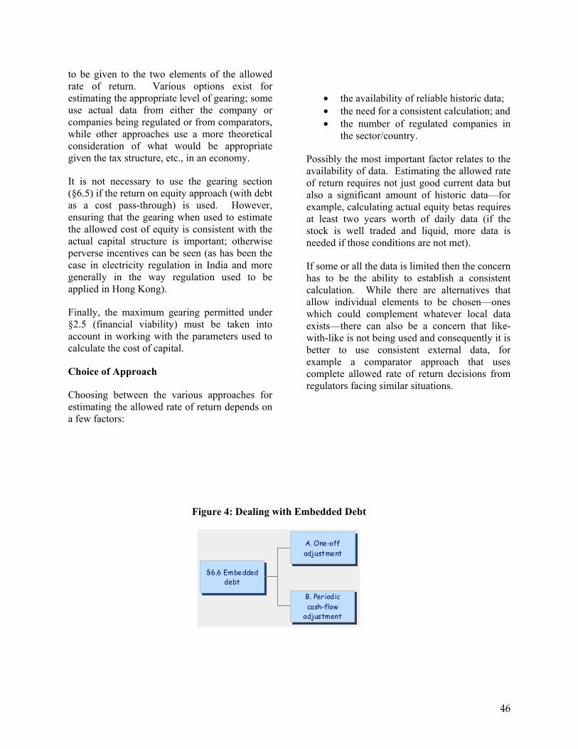
46
to be given to the two elements of the allowed rate of return. Various options exist for estimating the appropriate level of gearing; some use actual data from either the company or companies being regulated or from comparators, while other approaches use a more theoretical consideration of what would be appropriate given the tax structure, etc., in an economy.
It is not necessary to use the gearing section (§6.5) if the return on equity approach (with debt as a cost pass-through) is used. However, ensuring that the gearing when used to estimate the allowed cost of equity is consistent with the actual capital structure is important; otherwise perverse incentives can be seen (as has been the case in electricity regulation in India and more generally in the way regulation used to be applied in Hong Kong).
Finally, the maximum gearing permitted under §2.5 (financial viability) must be taken into account in working with the parameters used to calculate the cost of capital.
Choice of Approach
Choosing between the various approaches for estimating the allowed rate of return depends on a few factors:
• the availability of reliable historic data; • the need for a consistent calculation; and • the number of regulated companies in
the sector/country.
Possibly the most important factor relates to the availability of data. Estimating the allowed rate of return requires not just good current data but also a significant amount of historic data—for example, calculating actual equity betas requires at least two years worth of daily data (if the stock is well traded and liquid, more data is needed if those conditions are not met).
If some or all the data is limited then the concern has to be the ability to establish a consistent calculation. While there are alternatives that allow individual elements to be chosen—ones which could complement whatever local data exists—there can also be a concern that like-with-like is not being used and consequently it is better to use consistent external data, for example a comparator approach that uses complete allowed rate of return decisions from regulators facing similar situations.
Figure 4: Dealing with Embedded Debt
§6.6 Embeddeddebt
A. One-offadjustment
B. Periodiccash-flow
adjustment

47
Finally, if the sector being regulated has only one company then there will be a need for external data to overcome the constraints on incentives problem that arises from using only data from the company being regulated.
Making the choice as to what is the best approach to use will involve considering each of these issues and then determining which approach, or combination of approaches, will best serve the situation faced by the regulator.
Financial Viability and Embedded Debt
Linked to the allowed rate of return issue is how to handle some one-off events. Two of these are considered: (a) the problem of inherited debt whose interest rate differs significantly from market rates (§6.6); and (b) the problem of a shift in interest rates (§6.7). The Guidelines include these two as variants—see Figure 4. The embedded debt problem should not arise; ideally governments address this issue when restructuring or privatization takes place. However, situations in which it is not addressed can be envisaged and also, if the guidelines are being used for other forms of PSP (as discussed in Section 2.2), there may be a need for this sort of adjustment. Of course, it is not necessary to make a change but this would imply some form of windfall for the operator—a positive one if the embedded debt was low cost or a negative one if the embedded debt was high cost. Since the likelihood is that the debt is low cost, the operator would benefit. If this is known before a bidding process for choosing the private operator then, provided a competitive process is achieved, the benefit should be transferred to the government.
Adjustments can either be made to the regulatory asset base (RAB—discussed in detail in Chapter 4) or an annual cash-flow adjustment can be made. Adjusting the RAB is simplest since it is a once-for-all change.42
42 Of course, if a discounted cash flow approach to determining the RAB has been adopted, the problem of embedded debt will not arise.
Similar problems can arise if there is a fundamental shift in interest rates. If rates shift downwards, the situation covered in §6.7, then at the next periodic review the WACC that is estimated will be below the cost of the previously borrowed funds. In normal circumstances the company would be expected to be in a position to renegotiate or refinance the existing loans, but that may not always be the case. Consequently, it is possible to allow an annual cash-flow adjustment to ensure the financial viability of the company and so allow it to make the interest payments on the existing debt. Of course, to ensure that the company has an incentive to refinance where possible, the allowance can be time bound, say for one or two price control periods (§6.7.1(d) provides options for setting this time bound approach).
It was decided to make the adjustment only if rates fall. If rates rise the operator will receive a bonus since existing debt will be cheaper than the cost of debt allowed in the WACC. However, rate rises have tended to be temporary and this asymmetric approach was adopted since an attempt to control the number of adjustments is appropriate and the critical concern is about the financial viability of the operator.
A final issue that might arise is how forward looking debt guarantees (whether implicit or explicit) from a government should be handled—this should be treated separately to the adjustment made for existing “cheap” debt. If a government, for some reason, decides to provide guarantees without charge or at subsidized rates (compared to market prices), the first issue would be to understand why they would choose to do this. Cases clearly arise where government guarantees can be important in the financing of the utility; consider the case of Network Rail in the United Kingdom where over £18 billion of private debt has been raised with a government guarantee. It is probably best to address across-the-board government guarantees of debt through the determination of the cost of debt. The guarantee would probably shift the company to the same credit rating as the government and consequently when considering what premium should be allowed over the risk-free rate this should be taken into account. If

48
only a part of the total debt is guaranteed then it may be better to have a separate cash-flow adjustment—similar in impact to the embedded debt adjustment made by Ofwat in 1999—that lasts for the life of that debt.
Further Issues
One final set of issue that are only hinted at in the Guidelines—in §6.8.5—are the issues that arise when internal group debt is included and debt is being handled as a cost pass-through. In this case it would be appropriate for the regulator to become more intrusive so as to ensure that close-to-market-rates are actually being charged for the internal debt (or at least that is all that is allowed to be passed on to consumers). If debt is treated as a cost pass-through and internal group debt is expected to be an issue, then further consideration of what rules would be needed has to be undertaken by the transaction advisers.
Summary
Given the importance of the WACC for remunerating existing (RAB) and future (capex) investments, it is appropriate to have detailed and comprehensive rules. Chapter 6 sets out a set of workable guidelines that, while not quite “best practice,” do incorporate many of the best practice ideas in a way that should be implementable even in situations with limited information.
This is, however, an area where the Guidelines will need significant modifications to make them appropriate to the situation faced.
CH7. Capital Maintenance Charge
Introduction
Chapter 7 of the Guidelines sets out the basis for the return of capital. The term “capital maintenance” is used rather than “depreciation” since the approaches used are wider than simple depreciation as seen from the usual accounting viewpoint.
It is important that regulators adequately provide for capital maintenance in setting tariffs. The user-pays principle is an important concept underlying pricing decisions, and so ensuring that users pay for the renewal of assets, while smoothing payments over time to stabilize tariffs, is a goal that should be achieved in determining the revenue requirement.
Furthermore, the capital maintenance charge is important since it is a primary source of funds for the operator—especially important when the company is faced with a major investment program. Consequently, any decisions about capital maintenance, especially as it relates to existing assets, should be viewed carefully from the perspective both of ensuring that customers pay for the services they consume (considering that providing the service reduces the ability of the assets to produce future services) and of the cash-flow position of the company.
Third Party Funded Assets
One key issue concerning capital maintenance is whether assets funded up front by third parties—customers or the government—should be included in the capital maintenance base. (We are concerned here only with one-shot funding—i.e., where the third party will not fund later renewals of the asset.) This issue arises in §7.1, with the proposal there being that all assets funded by customers and government should be subject to a capital maintenance charge.43
Before looking at this issue more closely, we should note that we are using the term “capital maintenance” broadly here to mean a charge of some kind that is treated as a cost in determining the revenue requirement and that reduces the RAB. Some regulatory experts would reserve the term “depreciation” (or “capital maintenance charge”) to mean the subsequent recovery by the company of capital investments financed by the company. So they would, by definition, exclude the charge we are considering from being called depreciation because it is, in effect, a 43 But not included in the RAB; see the discussion in Section CH4 of the Explanatory Notes to the Guidelines and Chapter 4 of the Guidelines.

49
prepayment by customers for asset renewal that the company will undertake in the future. We will ignore this matter in the following discussion; readers can substitute another term in place of “capital maintenance” below if it fits better with their concepts.44
As a preliminary point, we should note that the entire concern in the debate over charging capital maintenance for third-party-funded assets is over the time-profile of tariffs. Ultimately, customers will indeed pay for the renewals; it is just a question of when they pay—which may also mean which customers pay.
Full recovery of costs (no more and no less) as an objective is assured because the capital maintenance charge (or another kind of charge that serves the same purpose), whenever it occurs, will reduce the RAB concurrently with bringing additional revenue. So the company does not receive a windfall (in NPV terms) by requiring customers effectively to prepay asset renewal.
Going beyond cost recovery, four relevant objectives in this context are the following:
(a) Giving the right price signal to customers (allocative efficiency in consumption).
(b) Intergenerational equity—not loading onto one particular generation of customers the costs of a service provided over the longer term.
(c) Increasing the likelihood that needed funding for timely renewals will be forthcoming.
(d) Regulatory simplicity.
It will be useful to look separately at government funding (we include here grants
44 For example, if the charge is instead treated as an advance from customers, it would give rise to a liability (deferred revenue) on the regulatory balance sheet, which would reduce the net RAB, with the same effect as if it were depreciation.
from development agencies—e.g., output based aid) and customer funding.
With respect to government funding, charging capital maintenance serves (a) and (b) well. If customers paid nothing for the asset until after the company replaced it, only the first cohort of customers would receive the benefits of the grant. By requiring customers to start paying for capital maintenance right away, the subsidy is effectively spread over all customers in perpetuity, since the average RAB will be reduced compared with the case in which the company charges nothing during the life of the initial asset and then has to finance the renewal itself.
An exception would be made in the case of government grants that are clearly aimed at providing a service to a targeted group of customers. In that case, it may be a policy not to charge capital maintenance to these customers.
The picture may seem different in the case of customer contributions. Customers who have just paid up front for an asset must begin right away to pay capital maintenance—effectively, a prepayment for renewal of the asset. This might appear to be double charging. Of course, over all customers, both present and future, this is not double charging since later customers will receive the benefit of the reduced RAB. But the burden may appear to fall disproportionately on those customers who provide the initial funding. The story is not so straightforward, however, since intergenerational smoothing could occur by the capitalization in property values of the initial customer investment.
In any event, in both cases objective (c) is well served by imposing a capital maintenance charge. In fact, a major rationale for imposing a charge in the case of third party-funded assets (regardless of whether the charge is labeled “depreciation” or an “advance from customers”) is a practical concern about the uncertainty of future funding from customers or the government for needed replacements. It is a simple reality in many countries that if the company is expected to find financing itself for the renewal of the assets, renewal may not take

50
place in a timely manner. There is likely to be an implicit expectation that someone else will provide the funding. In contrast, if all assets are treated the same way with respect to capital maintenance, a strong signal is given that replacement is the responsibility of the company—and requiring prepayment addresses the potential concern about financial viability. This also ties in with objective (d), above: the regulatory system is kept simpler if a general rule is adopted according to which all assets enter into the capital maintenance base (although, as noted above, they do not necessarily enter into the regulatory asset base).
Moreover, this approach can also remove perverse incentives for the company to either accelerate or decelerate replacement programs for third-party-funded assets. Given the likely investment needs for the company, anything that helps ensure the timely funding and implementation of what may be considered lower priority investment deserves consideration as a useful tool.
Another aspect to consider is that optimal asset renewal expenditures generally do not appear only suddenly at the end of the stipulated life of the asset. Major repairs and overhauls that go beyond opex may be needed much earlier. So reference in the paragraphs above to “prepayment” may not be quite right: to some degree, these payments by customers will meet current expenditures by the company.
A similar idea lies behind the network renewals charge that has been proposed in the Guidelines as a substitute for depreciation in the case of underground assets (see below). This charge covers all underground assets, including those funded by third parties.45 The reason is that this kind of capex is considered to be like ongoing
45 This is consistent with how the infrastructure renewals charge works in England and Scotland. Government grants for network assets are not written over time to the profit and loss account (as they are in the case of assets subject to depreciation) and so customers would immediately begin paying the incremental renewals charge on any government funded network assets.
heavy maintenance rather than the replacement of discrete assets at the end of their useful lives.
Whatever the approach taken, the essential message is that the rules governing capital maintenance, covering assets initially funded in the different ways, should be set out clearly and comprehensively. This is often not done.
Network Renewals Charge
There is a group of assets for which it is difficult to determine exactly over what period the assets should be depreciated. For underground assets it is often difficult to determine an exact asset life—some assets have been providing a service for over 100 years in parts of the England & Wales system. Consequently, an approach has been developed that focuses on the cost of maintaining the assets in a state sufficient to deliver the service, rather than trying to determine a period over which the assets can be depreciated. This is set out in §7.2.
This alternative approach makes use of a network renewals charge, which can be estimated in several different ways. Some of the options require significant information—some of which may not be available or, if it is available, may not be sufficient. For example, the original approach to network renewals in England & Wales focused on considering the average expenditure on maintaining the underground assets over the last 20 years—a period believed to be sufficiently long for any cyclical or discretionary expenditure to be suitably averaged.46 However, if the expenditure over that period was not sufficient to actually maintain the assets, all that would be done is to establish a system that continues to under-fund capital maintenance.
To make a network renewals charge approach work in a reduced discretion environment two options are presented. The key is how much information is available about expected capital maintenance requirements—when only limited information is available then a review needs to be mandated. When the review can take place is 46 Referred to as the “long-run normative charge”.
51
something that the transaction advisers should establish and then adjust §7.2.3(c) accordingly. Guidelines for how the review should be undertaken are also provided.
An important relationship will also exist between network renewals and backlog investment. Guidelines for how this relationship should be handled in the initial price control periods are also provided.
Above-ground Assets
Section 7.3 provides two approaches to handling the above ground-assets. The first is a traditional approach based on the asset value and commercial life of the asset. A second approach is to use the initial value of the RAB as the starting point for depreciating the above-ground assets (the initial RAB is discussed in Section CH4 of the Explanatory Notes to the Guidelines and in Chapter 4 of the Guidelines). The choice partly depends on the choice of initial RAB and the implications that the different options have both for consumers (via the price level) and investors (through the cash-flow generated by the capital maintenance charge).
In both cases it is suggested that no change can then be made to the depreciation charge (before price indexation)—effectively the unindexed asset value and the commercial life are fixed once determined.
For new above-ground assets a process is provided for determining an allowed depreciation charge which can be changed—but only at a periodic review determination.
Concessions
One twist that needs to be addressed arises when limited-duration concessions with no terminal value are being regulated. When assets with a commercial life greater than the remaining life of the concession are acquired, the depreciation charge is set to recover the asset value over the shorter remaining life of the concession, so ensuring no terminal value for the asset (§7.4.1). In effect, a system of accelerated depreciation is created.
A concern that arises with accelerated depreciation is the impact that this can have on prices. Consequently guidelines are also provided (§7.4.3) for determining when this is appropriate and options that can be followed (without creating a terminal value) if the variation in prices would be too great.
CH8. Capital Expenditures (Capex)
This is one of the most difficult areas since there is often great uncertainty about what investment will be needed during a price control period—let alone the medium-term. Furthermore, this is an area where regulators often feel most exposed due to the information asymmetry they face—both with respect to the need for investment as well as the appropriate cost to allow. Additionally, companies can feel exposed over capex since they face the risk of regulatory hold-up which can be more significant as more investment is undertaken. As such, while rules have been established, they are as much concerned with process as with specific solutions to problems.
At the beginning of the Explanatory Notes to the Guidelines we noted the generic problem of information and the need to have good accounting systems as well as established templates, etc. Capex is an issue where these information systems are especially important. A major part of the business plan, due to be submitted prior to a price determination, has to deal with capex—this is discussed further below.
Finally, a key concern with capex is creating sufficient incentives for the managers of the company to strive to deliver the capex program as cheaply as possible. A major part of this chapter of the Guidelines is concerned with the different options available for creating incentives. These are discussed below, as well as in more detail in Alexander and Harris (2005).
Determining the Capex Program
§8.2 sets out some of the procedures needed for collecting the information necessary to determine what capex is required over the price

52
control period. The regulator must provide clear signals as to what objective there is for the program (§8.2.1) and then the company is expected to respond through the business plan. §8.2.2 and §8.2.3 set out some of the issues that the regulator should consider when assessing the capex program proposed by the company.
The way in which information is presented and some of the concerns linking asset condition and performance are set out in Annex 1 to this Explanatory Notes to the Guidelines.47 The sort of categorization and approach provided in the Explanatory Notes to the Guidelines would be helpful as part of the business plan and consequently consideration should be given to the regulator amending the detail of the tables in the annex and providing something like this as a template for companies. Furthermore, by establishing a process by which capex is categorized the framework can help the company and regulator reach agreement on the capex program—or at least hopefully minimize the areas where disagreement exists.
While forecasting capex is important, there is always the fall-back position of ERs for unanticipated major capex (Chapters 9 and 10). These provide an option for dealing with major unanticipated capex, such as environmental capex arising from new obligations imposed on the sector.
Later Adjustments to the RAB
The core incentive for minimizing the cost of capex once the program has been agreed lies in the way in which the forecast capex figures are replaced with actual figures. Section 8.3 sets out the main approaches that are likely to be
47 While the approach outlined in Annex 1 is helpful, it is based on the existing system in England & Wales, which has been criticized, especially with respect to underground assets, inasmuch as the system used (represented by the tables in the annex) do not distinguish sufficiently clearly between the issues of asset condition and service performance. These are areas that require further work to make the tables more appropriate for other countries that might use them.
needed—different types/classes of capex are likely to need different approaches and consequently several of these options are likely to have to be incorporated in the final version of the guidelines proposed by the transaction advisers.
There are two basic approaches provided:
• Ex ante ex post. This is the standard where a forecast (ex ante) figure is employed when undertaking the price determination and then the actual (ex post) is used to replace the number at some point in the future—these options are set out in §8.3.4 variants A to C. The choice of date for replacing the figure has an important impact on the incentives faced by the operator. The focus in the United Kingdom has now been on a rolling system such that efficiency savings are always kept for five years. Only one of these variants should be used in the final set of regulatory rules.
• Cost pass-through. Here a range of approaches is available with the options set out in §8.3.7, §8.3.8 and §8.3.9. The options relate to the degree of cost pass-through. There can be total pass-through or partial pass-through. Under the partial pass-through systems either the cost per unit or number of units of investment is fixed, so providing some incentive for the company while allowing the less controllable aspect to be passed-through. One, all or none of these variants could be used in the regulatory rules adopted.
The transaction advisers will need to determine which types of capex will be subject to which form of control, the key criteria for the choice being:
• Is the capex controllable (under the cost control of the company and subject to control over the timing of the investment)?
• Can the capex be predicted—more from a forecasting perspective than a controllability one?

53
• Is the class of capex material?
A final issue that has been included with the pass-through approaches is the idea of having a budget or ceiling for the capex. Since some control vis-à-vis the price level is desired it is still necessary to forecast a level of capex, even for the pass-through items. Then, to ensure that the company does not have a perverse incentive to over-invest (say, because another element of the price control is a little generous), a budget for the capex can be set. Whether this is a hard budget or one that signals a prudency review is a question that will have to be decided, but it does provide some certainty to the regulator and customers about how prices are likely to move.
Logging-up
An alternative approach which could be employed either if no pass-through system is implemented or if a hard budget constraint on the pass-through fund is set is that of logging-up. §6.4 sets out how the approach could be made to work. The basic approach is one where the company receives no allowed return (WACC) or capital maintenance on the investment during the price control period in which it was undertaken. Rather, at the next price determination the capex is incorporated as though it was undertaken at year 0 of the new control period—with the financial carrying costs of the capex included in the investment cost. This leaves the company in an NPV-neutral position. Of course, this approach only works if the company is financially strong enough to fund the investment until the next price control period.
Ex post Prudency Test
Something that is necessary for most of the approaches to capex is a prudency test. This can be applied when:
• the ex post cost of a project is greater than the ex ante forecast;
• the pass-through ceiling is breached; or • logging-up is used.
Section 8.5 provides some guidelines for how an ex post prudency test should be undertaken. They err on the side of the company inasmuch as they provide a test based on how another “reasonable” operator would have acted. However, they do provide comfort for the regulator and consumers in that several key criteria are provided for the assessment. Further, there is a strong push towards market-determined prices through competitive procurement of capex. If a company can demonstrate a competitive procurement was followed then the cost of the investment is not questioned (although the timing and need could still be queried).
There are also guidelines to allow for small over-runs to be passed through without a prudency test.
CH9&10. Extraordinary Review
Events That Qualify as Extraordinary Events
This chapter falls outside the core scope of the Guidelines, which deal with the periodic price review. ERs are built into the regulatory process to deal with unanticipated events that have major cash flow consequences for the company which make it inadvisable to wait until the next periodic price review to make needed tariff adjustments.
ERs are used in typical concession contracts and in conventional utility regulation. Ofwat refers to them as “interim determinations”.48
There are different approaches to how to define the kind of event that will trigger an ER. One approach is simply to state the underlying principle: any event that could not reasonably have been anticipated at the time of the last price review, or that was not taken into account at the last price review (or something along these lines). The disadvantage is that disputes can
48 Meaning “interim determination of K,” where K is the profile of tariff increases. See Alexander and Harris (2005) for more on Ofwat’s interim determinations.

54
easily arise over whether or not the principle applies in a specific case.
Another common approach is to list types of events and state that only these specific events can trigger an ER. If this approach is taken, typical events that might be covered are the following:
• a change in law (this can be made narrower by limiting it to certain types of law—laws or regulations that relate directly to water or wastewater services, the environment, etc.);
• a change in the required service or performance standards;
• a change in the service area;
• a change in the volume of water sold by more than a certain percentage (but this would not be needed if the rules provide for automatic volume adjustments).49
If the regulator is considered to be reasonably competent and fair (e.g., it has established a good track record) and the appeals procedure gives considerable deference to the regulator’s decisions, it is probably best to include the catch-all clause in addition to a specific list of types of events. This will prevent situations in which an adjustment is clearly warranted because of a highly unusual event that, however, does not figure in the list of specified events.
The regulator might also include specific events as part of the price review—i.e., where they are too uncertain to be included as fixed values in the revenue requirement but probable enough to be provided for explicitly on this contingent basis. (Ofwat refers to these as “notified items”—e.g., differences in the number of customers opting for meters, relative to the assumptions made at the price review.)
49 Automatic adjustments in the average tariff for changes in the volume of water sold are discussed in Chapter 2, based on the breakdown of opex into fixed costs and volume-related costs in Chapter 3.
The present Guidelines do not cover the question of which events qualify. They pick up once an extraordinary event has occurred. But there is one important qualification. Regardless of the type of event, the impact of the event (i.e., the tariff adjustment that would result from it) must exceed a specified materiality threshold; otherwise no adjustment is made (§10.5.2).
The Process of the Extraordinary Review
With respect to ERs, the Guidelines deal with both process and methodology. This is in contrast with the other sections of the Guidelines, which do not deal much with process aspects (not because these are not important but simply because of the narrower scope of this project).
Much of Chapter 9 (process) is straightforward, describing how the review is initiated, the kinds of information that must be submitted, the regulator’s draft determination and its review by the company, and the regulator’s final determination, involving a tariff adjustment that takes place in the near future—before the next periodic price review.
Two of the provisions in Chapter 9 are more unusual—in particular:
• The Guidelines discourage both the regulator and the company from initiating the ER process if they do not feel fairly sure that the materiality condition (§10.5.2) will be satisfied. Whichever one initiated the process will have to pay the costs the other incurred during the review if it turns out that the materiality threshold was not exceeded (§9.6.1).
• The company is given some discretion over the profile of the needed tariff adjustments, so long as the present value of the expected revenue is not affected (§9.7.3). Constant tariff adjustments in each year are always acceptable, and in certain circumstances the needed tariff adjustments can increase over the remaining years of the control period.

55
Methodology
Chapter 10 sets out the methodology for carrying out the tariff adjustments in an ER. One way to make these adjustments would be redo the tariff determination made at the most recent periodic price review, now with hindsight knowledge of the extraordinary event—but looking only at the impacts of the extraordinary event (i.e., this is not a mini periodic review). This is the method used by Ofwat.
The Guidelines present a different kind of method as an alternative (and not necessarily to replace a method more closely related to that used by Ofwat). The method in Chapter 10 cleanly separates the tariff as determined at the last review from the incremental tariff adjustment (positive or negative) due just to the extraordinary event. This has the advantage of avoiding the need to revisit the past price review. Even though in the context of low-discretion rules, it should be clear what values from the past can and cannot be modified, in some circumstances opening up the past might be a dangerous exercise if, by merely having the values on the table once more, there is greater scope for argument over whether various past values should be revised in the light of what has occurred since then.
The basic methodology for determining the required tariff revenue is simply to find an incremental tariff profile (positive or negative, depending on the extraordinary event) that is expected to result in additional revenue whose present value is equal to the present value of the incremental costs (§10.5.4). This is a method commonly used in concession or public-private partnership agreements. The main difference in the method given in the Guidelines is that it takes into account the periodic overall price reviews that will take place. Adjustment methods sometimes do not do this, with the result that each ER results in an incremental tariff that continues for the remaining life of the concession—with the result that after a few years and even after the next price review, the total tariff will consist of the basic tariff plus a set of incremental tariffs resulting from various ERs in the past. This is cumbersome.
So the method given in the Guidelines determines a terminal value at the end of the current price control period, representing the value that has not been recovered through revenue during the current control period (i.e., the depreciated value of the assets at that time). This value is then simply added to the opening RAB for the next control period (§10.5.7) and the ER tariff adjustment, as such, disappears. The Guidelines specify that cost recovery is to take place on a constant real annuity basis (§§10.4.3 et seq.) over the asset life; so the depreciated value (terminal value) at the end of the control period equals the present value of the annuity “payments” that would have been made in future control periods (easily calculated using the “PV” function in Excel).
Materiality Threshold
As noted above, Chapter 10 includes a materiality threshold (§10.5.2). On a present value basis, the absolute value of the revenue adjustment during the current control period must exceed a specified percentage (perhaps 1 to 5 percent) of the revenue requirement as determined at the most recent price review; otherwise the tariff adjustment will not be made. This is consistent with the rationale for the ER—i.e., to deal with events that have a cash flow impact significant enough not to be postponed to the next price review. Note that if the value does not pass the ER materiality test, it may be eligible for logging up under the provisions of Chapter 6 (§8.4.2(b)(i)), in which case the adjustment would be postponed until the next price review and financial carrying costs would be included.
CH11. Use of Independent Experts
Different Ways of Using Expert Recommendations and Decisions
The topic of dispute prevention and adjudication is not strictly within the scope of the present project, but since independent experts play a critical role in some parts of the Guidelines, a short chapter has been included to deal with this

56
(Chapter 11). It is an important subject, and much more attention needs to be given to it than is included in this sketchy chapter—and than is included in the typical concession contract.
Of course, the advice and opinions of experts are frequently solicited and used by regulators. What distinguishes the role of experts in Chapter 11 is that their decisions are binding on the regulator. This practice is less common.
The important distinction in using the term “expert” is that in many legal systems determination of issues by experts is not considered under law to be arbitration. Most countries have special laws dealing with arbitration and, although given greater deference by the judicial system, arbitration often offers less flexible procedures than expert determination. (To the extent that in a particular country, arbitration can be used in the way envisaged in Chapter 11, the distinction may break down and what is written in that chapter could apply to specialized forms of arbitration, too.)
Determination of issues by independent experts can take place in a number of different ways. At one extreme, experts (as opposed to an arbitral or appeals tribunal) can be used to decide any issue about which the company and the regulator disagree—or a broad range of issues. One problem is that some public authorities might find this solution objectionable, especially if the dispute involves policy aspects. Experts may be able to decide issues more quickly and at less cost, but they may not have the same aura of institutional acceptability.
This role of experts is sometimes included in concession-type contracts for certain categories of issues or, in an advisory way, as a preliminary step before adjudication by an arbitral tribunal or courts. Alternatively, experts can be engaged to give an advisory opinion, which is made public, before the regulator considers the issue and takes a decision. This can be especially useful for a new and untested regulator that could benefit from independent support for its decisions.
Another approach would be to limit the use of expert determination to certain well-defined issues. For all other issues, disputes would be treated by whatever the normal “appeals” procedure is (appeals court, international arbitration, etc.). When this approach is adopted, rule designers have to deal with new issues that arise—e.g., who decides a dispute over whether the issue is indeed one that is subject to expert determination, and whether the carve-out leaves important subissues outside the expert’s purview. Careful drafting is required. In addition, it should be considered whether all such issues arising in a price review should be submitted to the expert at the same time for convenience and cost savings. At the very least, all related issues must be submitted at the same time.
Expert panels have been used extensively in public service concessions in Chile, for matters ranging from tariff reviews (tariff level itself or specific assumptions used in calculating tariffs), fines, quality standards, and investment obligations.50 There appears to be a consensus that this approach has been successful.
Use of an Expert Panel to Manage and Facilitate the Entire Price Review
An idea that would fit nicely with the Guidelines would be to engage several experts (an “expert panel”) for the entire duration of the price review exercise. The expert panel would not itself carry out the price review; that would be the task of the regulator. Instead, the experts would help facilitate the review, even before there is any dispute, by discussing issues with the two parties as they arise, helping to resolve misunderstandings, etc. The panel could be given a proactive role in managing the review process. Procedures would be developed for this. And then, most important, when the regulatory rules call for this (and only at those points in the rules where this is called for), the experts would be empowered to take binding decisions. This would be a highly structured
50 See Jadresic (2006).

57
system of expert facilitation and determination.51 It is probably in this context that the idea of experts having the power to decide only a number of narrow issues makes the most sense.
Provisions for Expert Determination Contained in the Guidelines
It would not have been manageable for these Guidelines to try to present all the ways that expert determination could work in this context. We have decided to take a minimalist position here: expert determination (in the sense of a binding decision) is used only for a few important decisions. The main criteria tend to be the following (not all are present for each instance):
• the issue is well-defined, limited in scope, and is easily separable from all other issues;
• it involves considerable discretion and hence requires a high degree of technical expertise and good, mature professional judgment;
• it is purely technical—public policy concerns should not enter into the decision;
• the outcome could potentially have a considerable impact on tariffs or company cash flow—i.e., it is not an insignificant item that could easily be dispensed with by a cruder low-discretion rule;
• if it is not decided quickly, it could block the effective carrying out of the price review—i.e., it is not something whose adjudication could easily be put off for months or years.
Using experts in this manner is one way to help reduce the discretion accorded to the regulator.
Three sections of the Guidelines (§11.1 to 11.3) serve merely as place-holders; no guidelines are actually given. (This is left for further work—
51 For a more extensive discussion of this topic, see Shugart and Ballance (2005).
extremely important work.) These place-holder sections would deal with:
• General provisions, governing all aspects from the appointment of the experts (and the designation of an “appointing authority”) and the procedures they will follow, to the final status of their decisions (e.g., the conditions under which, and the extent to which, they can be challenged). This section would also need to set out clearly who bears the cost of expert intervention (and whether the cost will be included in the revenue requirement) for different kinds of interventions and perhaps for different outcomes.
• Specific provisions dealing with how the panel would intervene when the regulator and the company have a disagreement about something.
• Specific provisions dealing with how the panel could be used to determine a particular value, without the parties attempting to reach agreement first. This approach is used in certain places in the Guidelines where there is a highly technical matter that needs to be determined.
Guidelines for Use of Experts in Selecting Comparators to Determine the WACC
Chapter 11 (§11.4) develops in more detail one particular way that expert determination could be used to facilitate the determination of various values needed for the WACC. One reason for developing these guidelines in more detail is to show that experts can be used in very specific and limited ways to prevent deadlock.
Chapter 6 of the Guidelines makes extensive use of comparators in the determination of the various elements of the WACC. §11.4 gives one example of how expert intervention could be use to deal with these narrow but critical and potentially high-discretion decisions: the selection of comparator companies for purposes of determining the value of beta to use in the WACC (§6.4.4, Variant B). The procedure involves choosing between five and 10

58
comparator companies and calculating the average of the beta values, as determined by regulators in their most recent price reviews. This value is then used for the company’s beta in the present price review. The method given in Chapter 6 breaks down the issue into several components, most of which are low-discretion in nature. Once the identity of the comparators is fixed, the calculations involve very little discretion—they are almost mechanical. The difficult step is choosing appropriate comparators. In the procedure given in §11.4, the regulator the company would propose and challenge comparators in several steps, with the expert intervening at specified points and taking the final decision.
Small modifications would need to be made to adapt this section to other similar comparator decisions needed in Chapter 6:
• Comparator companies for the determination of the debt premium (§6.3.5).
• Comparator companies for the determination of optimal gearing (§6.5.3).
• Comparator countries for the determination of the risk-free rate (§6.2, Variant B).
• Selection of regulators for the determination of the market risk premium (§6.4.2).
The procedure in §11.4 would probably make sense only if it were included in a broader, facilitating role for the expert or an expert panel, as noted above. The expert would work with the staff of the regulator to determine the required values, interacting with the company at certain key points. Determination of intermediate and final values would be the responsibility of the regulator (this would be important for political perception), but the expert would have the power to decide certain issues involving the choice of comparators.
We believe that more attention should be given to mixed solutions such as this one, where experts can help move the process along and prevent deadlock over critical sub-issues, while avoiding the negative perception that an entire matter of important public interest has been simply handed over to outsiders (and in some cases, foreigners) to decide.
The procedure in §11.4 is developed in considerable detail because of the importance of the outcome. It would not make sense to use a procedure of this complexity for a decision that could have much less impact—and hence would be much less contentious.
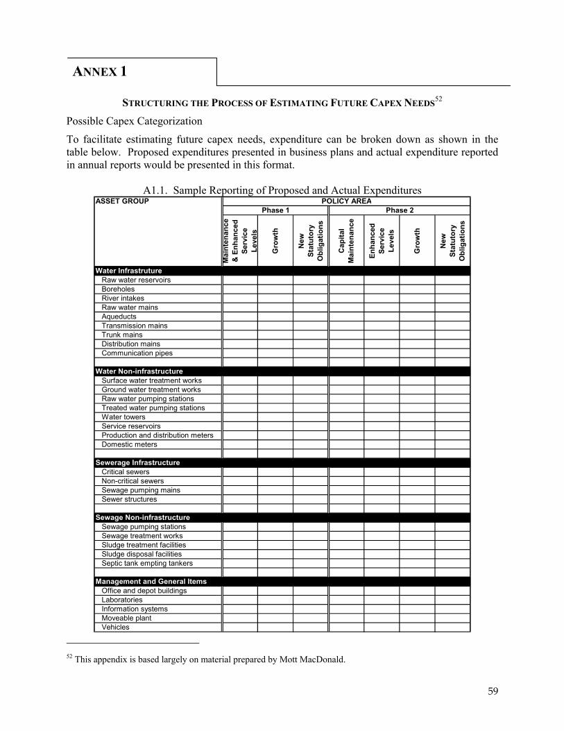
59
ANNEX 1
STRUCTURING THE PROCESS OF ESTIMATING FUTURE CAPEX NEEDS52 Possible Capex Categorization
To facilitate estimating future capex needs, expenditure can be broken down as shown in the table below. Proposed expenditures presented in business plans and actual expenditure reported in annual reports would be presented in this format.
A1.1. Sample Reporting of Proposed and Actual Expenditures ASSET GROUP POLICY AREA
Phase 1 Phase 2
Mai
nten
ance
&
Enh
ance
d Se
rvic
e Le
vels
Gro
wth
New
St
atut
ory
Obl
igat
ions
Cap
ital
Mai
nten
ance
Enha
nced
Se
rvic
e Le
vels
Gro
wth
New
St
atut
ory
Obl
igat
ions
Water InfrastrutureRaw water reservoirsBoreholesRiver intakesRaw water mainsAqueductsTransmission mainsTrunk mainsDistribution mainsCommunication pipes
Water Non-infrastructureSurface water treatment worksGround water treatment worksRaw water pumping stationsTreated water pumping stationsWater towersService reservoirsProduction and distribution metersDomestic meters
Sewerage InfrastructureCritical sewersNon-critical sewersSewage pumping mainsSewer structures
Sewage Non-infrastructureSewage pumping stationsSewage treatment worksSludge treatment facilitiesSludge disposal facilitiesSeptic tank empting tankers
Management and General ItemsOffice and depot buildingsLaboratoriesInformation systemsMoveable plantVehicles
52 This appendix is based largely on material prepared by Mott MacDonald.

60
Asset Condition and Performance Grading
Assessing the condition and performance of assets is a means of assessing the capital maintenance needs for those assets needed for the long term. Asset condition is assessed through surveys of assets using descriptive grading systems at a point in time. For above-ground assets, condition data can be collected quickly. Below-ground assets are more difficult to inspect, (requiring CCTV of sewers and sampling of water mains) and consequently it takes longer to acquire condition data for a reasonable coverage of the networks (normally between three to five years).
Performance data (for example bursts per 1000km of pipe) needs to be collected over a period of time, a minimum of one year and preferably three to average out annual variations. Combining the condition and performance data in a 5×5 matrix gives a picture of the assets in worst condition, as follows: The assets that are assessed to be condition grade 5 (essentially defunct and requiring replacement within 5 years) and performance grade 5 (failing frequently and therefore incurring high reactive maintenance costs) are assessed to be in the worst state and are targeted for renewal.
Note the asymmetry: an asset that will require replacement within a few years (at the most) but that, for the moment, shows excellent performance (Condition 5, Performance 1) ranks higher in priority than an asset in excellent condition but that is performing very poorly (Condition 1, Performance 5). The reason is that, if poor performance is not caused by the poor condition of the particular asset, it is likely that replacement of that asset will not be the optimal solution.
In the context of negotiating a concession, if condition data is available for all assets, then it will be possible to assess the proportion of each asset type that is in condition grades 1, 2, 3, 4 and 5. If this is combined with an assessment of asset values (modern equivalent asset values) by type of asset, then it is possible to assess the proportional values in CGs, 1, 2, 3, 4 & 5. A rough-cut estimate of the next five-year maintenance needs could then be assessed as the aggregate value
A1.2. Condition of Assets Condition
Performance
1 Excellent
2 3 4 5 Defunct
1 Excellent
2
3
4
5 Poor

61
of the condition-grade five assets. In practice, this tends to lead to a high estimate, as a proportion of CG5 assets are more economic to replace on failure than to replace proactively through capital maintenance.
One further use of condition and performance grades is that if assessments are repeated over time, provided that the same methods are used, they may give a measure of asset deterioration. This can support a more forward-looking approach to asset maintenance (rather than just focusing on known problems) and facilitates whole-life costing and forecasting of asset performance and impacts on customer service.
Examples of Grading Systems
Examples of condition grading and performance grading systems are provided for water-mains and above-ground assets (see Tables 1 to 4). In practice, more asset-specific descriptions, perhaps supported with photographs, are used for different asset types (e.g., service reservoirs, pumps, HV electrical equipment, etc).
In a concession context, it would be up to advisors to develop appropriate grading systems for the types of asset being maintained. If the Regulator wants the concessionaire to assess condition in an objective and consistent way, perhaps on a periodic basis as part of its monitoring duties, then the grading systems would need to be issued as information requirements and the assessments themselves audited. This will be particularly important if assessments of asset condition and performance form part of the handover arrangements, to avoid arguments over the interpretation of the condition grades.
Limitations of Condition and Performance
Although a helpful indicator of investment need, condition and performance matrices have their limitations:
• Condition assessments can be subjective and it is often difficult to get wholly repeatable results from different assessors, even with training. Sample audits are always needed to check consistency;
• Owing to the first limitation, Regulators (e.g., Ofwat) often feel free to ignore condition-based arguments for investment;
• The link between condition and service to customers is often weak and many CG5 assets are more economic to deal with reactively, rather than proactively. For example, as a 300mm diameter water main will affect more customers when it fails, than an 80mm diameter main, it may warrant more urgent attention than the 80mm, even though it may be in better condition;
• For assets that have received no maintenance for many years, there may be a high proportion of poor condition assets. This can result in the map being colored red with CG5 assets and an investment plan based on replacing CG5 assets in the first five years becomes wholly unaffordable. This is unhelpful and other methods of discrimination are needed.
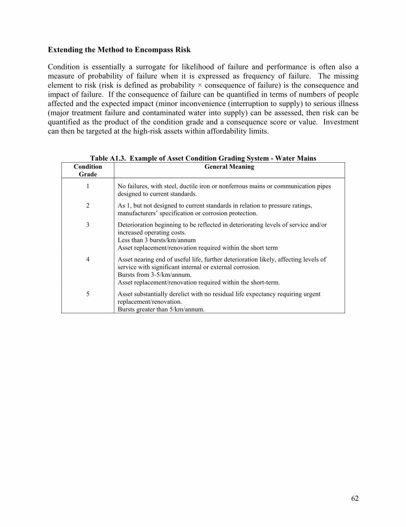
62
Extending the Method to Encompass Risk
Condition is essentially a surrogate for likelihood of failure and performance is often also a measure of probability of failure when it is expressed as frequency of failure. The missing element to risk (risk is defined as probability × consequence of failure) is the consequence and impact of failure. If the consequence of failure can be quantified in terms of numbers of people affected and the expected impact (minor inconvenience (interruption to supply) to serious illness (major treatment failure and contaminated water into supply) can be assessed, then risk can be quantified as the product of the condition grade and a consequence score or value. Investment can then be targeted at the high-risk assets within affordability limits.
Table A1.3. Example of Asset Condition Grading System - Water Mains Condition
Grade General Meaning
1 No failures, with steel, ductile iron or nonferrous mains or communication pipes designed to current standards.
2 As 1, but not designed to current standards in relation to pressure ratings, manufacturers’ specification or corrosion protection.
3 Deterioration beginning to be reflected in deteriorating levels of service and/or increased operating costs.
Less than 3 bursts/km/annum Asset replacement/renovation required within the short term
4 Asset nearing end of useful life, further deterioration likely, affecting levels of service with significant internal or external corrosion.
Bursts from 3-5/km/annum. Asset replacement/renovation required within the short-term.
5 Asset substantially derelict with no residual life expectancy requiring urgent replacement/renovation.
Bursts greater than 5/km/annum.

63
Table A1.4. General Classification for Above Ground Assets
Condition Grade
General Meaning
1 Sound modern structure with modern mechanical and electrical plant and components that are operable and well maintained.
2 As 1, but showing some minor signs of deterioration. Routine refurbishment and maintenance required with review of condition in the medium-term.
3 Functionally sound, but appearance significantly affected by deterioration, structure is marginal in its capacity to prevent leakage, mechanical and electrical plant and components function adequately but with reduced efficiency and minor failures. Review of conditions required during the medium-term.
4 Deterioration has a significant effect on performance of asset, due to leakage or other structural problems, mechanical and electrical plant and components function but require significant maintenance to remain operational. Will require major overhaul/replacement within medium-term.
5 Serious structural problems having a detrimental effect on the performance of the asset. Effective life of mechanical and electrical plant and components exceeded and incurring excessive maintenance costs compared to replacement cost due to unreliability. Mechanical and electrical plant may be outdated design posing more potential health and safety risks compared to its modern equivalent. Mechanical and electrical plant may have key components for which lack of spares poses a serious risk of loss of station output. Will require major overhaul/replacement in short-term.
Table A1.5. Service Condition Indicators - Water Mains
Service Condition
Grade
Description General Meaning
1 Excellent Smooth bored mains and communication pipes not subject to corrosion or with sound factory applied linings, no level of service problems.
2 Good As 1, but with loose deposits that are noticeable under abnormal flow conditions, slight tuberculation which may give a rough surface, but does not substantially reduce the cross-sectional area of the pipe. May require routine flushing or air scouring.
3 Moderate Some problems with loose deposits or deterioration of linings leading to occasional complaints. Risk of quality failure, pipe with tuburculation causing up to 20 percent blockage by encrustation.
4 Borderline Frequent problems causing complaints, water quality known to have failed on more than one occasion under normal operating condition during previous twelve months. Mains with tuberculation causing 20-40 percent blockage by encrustation.
5 Fail Main suffering severe problems of infestation and loose deposits. Water quality cannot be ensured. Mains with tuberculation causing 60-80 percent blockage by encrustation.

64
How well does asset or asset group fulfil the intended function in terms of quality, capacity or serviceability.
Table A1.6. Above Ground Assets
Service Condition
Grade
General Description
General Meaning
1 Excellent (100 percent on all
aspects)
Meets all design and statutory requirements at all times and under all demand conditions. Meets company’s internal standards at all times in terms of performance and serviceability.
2 Full Serviceable (100 percent on key aspect or
> 95 percent on other aspects)
As 1, but shows minor performance shortcomings in noncritical aspects or under extreme demand or climatic conditions.
3 Normally Serviceable (Equivalent to >90
percent on all aspects)
Asset meets all statutory and performance criteria under all normal conditions but has minor shortcomings under extreme operational or climatic conditions.
4 Unsatisfactory (Equivalent to >75
percent on all aspects)
Performance or operational shortcomings have a significant effect on asset function/effectiveness when capacity exceeds 115 percent of average throughput or major shortcoming on one or more key aspects.
5 Unacceptable (Equivalent to <75
percent on all aspects)
Substantially incapable of meeting externally imposed and company’s internal standards except under normal or reduced operating conditions.

65
REFERENCES (N.B. Full references to documents cited in the Guidelines are included in footnotes in that document.)
Documents Cited in the Explanatory Note to Guidelines Alexander, Ian. Forthcoming. Cost of Capital: A Practical Guide for Infrastructure Regulators.
Alexander, Ian and Clive Harris. 2005. The Regulation of Investment in Utilities: Concepts and
Applications. World Bank Working Paper 52.
Alexander, Ian and Chris Shugart. 2000. “Risk, Volatility and Smoothing: Regulatory Options for Controlling Prices.” (http://www.geocities.com/ian_alexander_1967/price_volatility.doc)
Baietti, Aldo, Kingdom, William and van Ginneken, Meike, May 2006. Characteristics of Well-
Performing Public Water Utilities, Water Supply & Sanitation Working Note No. 9. The World Bank Cubbin, John. 2004. “Assessing Ofwat’s Efficiency Econometrics.” A report for Water UK. March. Dinar, Ariel, ed. 2000. The Political Economy of Water Pricing Reforms. World Bank. (http://www-
wds.worldbank.org/servlet/WDS_IBank_Servlet?pcont=details&eid=000011823_20050801131331) Eberhard, Anton 2007. Is it possible to regulate state-owned utilities effectively? Presentation at the
PURC/World Bank International Training Program on Utility Regulation and Strategy. Gómez-Ibáñez, José. 2007. Alternatives to Infrastructure Privatization Revisited: Public Enterprise
Reform from the 1960s to the 1980s. November. The World Bank.
Green, Richard and Martin Rodriguez Pardina. 1999. Resetting Price Controls for Privatized Utilities: A Manual for Regulators. EDI Development Studies. The World Bank.
Groom, Eric, Jonathan Halpern, and David Ehrhardt. 2006. Explanatory Notes on Key Topics in the Regulation of Water and Sanitation Services. June. The World Bank.
Irwin, Tim and Yamamoto, Chiaki, February 2004, Some Options for Improving the Governance of
State-Owned Electricity Utilities, Energy and Mining Sector Board Discussion Paper No. 11, The World Bank.
Jadresic, Alejandro. 2006. “Expert Panels in Regulation of Infrastructure in Chile.” Paper presented at
the 3rd AFUR Annual Conference, Windhoek, Namibia, March.
Komives, Kristin, Vivien Foster, Jonathan Halpern, and Quentin Wodon. 2005. Water, Electricity, and the Poor : Who Benefits from Utility Subsidies? World Bank. (http://www-wds.worldbank.org/servlet/WDS_IBank_Servlet?pcont=details&eid=000160016_20051121111548)
Matsukawa, Tomoko, Robert Sheppard and Joseph Wright. 2003. Foreign Exchange Risk Mitigation for Power and Water Projects in Developing Countries. Energy and Mining Sector Board Discussion Paper No. 9. The World Bank. December.

66
Pardina, Martin, Schlirf, Richard and Groom , Eric. 2008. Accounting Infrastructure Regulation – An Introduction. The World Bank.
Shugart, Chris and Tony Ballance. 2005. “Expert Panels: Regulating Water Companies in Developing Countries.” (http://rru.worldbank.org/PapersLinks/Open.aspx?id=6366).
Trémolet, Sophie and Jonathan Halpern. 2006. Regulation of Water and Sanitation Services: Getting Better Service to Poor People. World Bank.
Vagliasindi, Maria. 2008. Governance for State Owned Enterprises, World Bank Policy Research Working Paper 4542.
World Bank. 2002. New Designs for Water and Sanitation Transactions: Making Private Sector
Participation Work for the Poor, Water and Sanitation Program and PPIAF. (http://rru.worldbank.org/PapersLinks/Open.aspx?id=1063)
World Bank. 2006. Approaches to Private Participation in Water Services: A Toolkit. (http://rru.worldbank.org/PapersLinks/Open.aspx?id=6791)

67
USEFUL WEBSITES GPOBA: www.gpoba.org
OFWAT: www.ofwat.gov.uk
General Useful References
Bakovic, Tonci, Bernard Tenenbaum and Fiona Woolf. 2003. Regulation by Contract: A New Way to Privatize Electricity Distribution? Energy and Mining Sector Board Discussion Paper No. 7.
Baldwin, Robert and Martin Cave. 1999. Understanding Regulation: Theory, Strategy and Practice. Oxford University Press.
Body of Knowledge on Utility Regulation (a comprehensive listing of useful books, papers and case studies). (http://bear.cba.ufl.edu/centers/purc/documents/ReferencesandNarrativesforweb_000.pdf)
Foster, Vivien and Pedro Antmann, 2004. The regulatory challenge of asset valuation: A case study from the Brazilian Electricity Distribution Sector. Energy Working Notes no. 2, World Bank.
Gray, Philip and Timothy Irwin. 2003a. Exchange Rate Risk: Allocating Exchange Rate Risk in Private Infrastructure Projects. Public Policy for the Private Sector. Note no. 266. World Bank. December.
Gray, Philip and Timothy Irwin. 2003b. Exchange Rate Risk: Reviewing the Record for Private Infrastructure Contracts. Public Policy for the Private Sector. Note no. 262. World Bank. June.
Newbery, David, 1997. Determining the asset base for utility price regulation. Utilities Policy Vol. 6, Number 1.
Newbury, David. 1999. Privatization, Restructuring, and Regulation of Network Utilities. Cambridge, MA: MIT Press.
Viscusi, W. Kip, John M. Vernon, and Joseph E. Harrington, Jr. 2000. Economics of Regulation and Antitrust. Cambridge, MA: MIT Press.
Whittington, Geoffrey, 1994. Current cost accounting: its role in regulated utilities. Fiscal Studies Vol. 15, Number 4.

Tariff Setting Guidelines A Reduced Discretion Approach for Regulators of Water and
Sanitation Services
A TECHNICAL GUIDE
PART TWO – TARIFF SETTING GUIDELINES

i
ORIENTATION 1. The Guidelines focus on the periodic price review and its later consequences. They do not cover all needed tariff adjustments. 2. These Guidelines are not intended to be “model clauses” for contracts or secondary legislation. They are far from complete. The objective is rather to provide material that can serve as a good starting point for policy makers, regulatory advisors, and a drafting lawyer to work together to prepare the needed legal instruments. The purpose is to set out the core ideas in a logical framework, along with the most important conditions and qualifications. 3. The Guidelines might best be viewed as starting heads of terms for a contract, or a term sheet for a financial agreement, or an initial working draft for secondary legislation. Variants better suited to the particular context are missing, details are not fully developed, the language is loose in many places, inconsistencies and gaps remain, many definitions are too vague, etc. But the Guidelines are at a stage where competent regulatory advisors, including a good drafting lawyer, will readily be able to identify the work that remains to be done. This was the objective in writing the Guidelines. 4. The Guidelines have been written in ordinary language to facilitate easy comprehension. They might well be revised in different ways by users adhering to differing traditions of legal drafting, and they might be translated into different languages. For these reasons, we have especially tried to avoid Anglo-American legalese. (In any case, plain language is the trend for contract and legislative language in many common law countries, with Australia and New Zealand in the vanguard.)53 5. Many procedural details have been omitted for simplicity—e.g., details of notices to be given, detailed sequences of procedural steps and timing. This should not be taken to imply that the regulatory process is not as important. 6. To keep the Guidelines simple, for the most part an end-of-year convention has been used for all cash flows. Rule designers might choose instead to use mid-point values or averages for certain variables. The needed adjustments to the formulas can easily be developed; they do not involve any new conceptual thinking. 7. In some cases, adjustments that should ideally be made during a price review, so that they can be included in the revenue requirement for the next price control period, cannot in fact be made at that time because the information needed for the adjustment will not be available until after the end of the last year of the current control period. To prevent the rules from becoming overly complicated, it has generally been assumed (unrealistically) that adjustments of this sort can take place at the time of the price review. 8. Variants are given for some sections or paragraphs. Major variants are identified by capital letters (A, B, …). For each instance, only one of the variants should be used in the regulatory rules that are adopted. Unless specifically mentioned, there is no connection between, say, Variant A in one section and Variant A in another section; they are independent. Of course, there may be other methods or approaches that could be used in addition to the variants given in the Guidelines. We have tried to select the variants that are most likely to be of use, and 53 See, e.g., the Plain English Manual issued by the Australian Government’s Office of Parliamentary Counsel (version 11 March 2003) and G.C. Thornton (1996) Legislative Drafting (Fourth ed.) (London: Butterworth).

ii
we explain our reasoning in the Explanatory Notes to the Guideline. In some cases, other less likely variants are mentioned in notes in the Guidelines. Variants are to be distinguished from different methods that apply under different circumstances, where all the methods would be included in the regulatory rules along with a switching rule that determines which method is applicable at any given time. 9. Text in italic font (with or without square brackets) gives short comments or indicates missing information or additional rules that may be needed. The italicized parts of the text should not be included in the actual regulatory rules. 10. Footnotes give short comments, often of a more technical nature. They can generally be ignored without loss of continuity. The footnotes should not be included in the actual regulatory rules. 11. The explanatory notes, which give longer comments, should not be included in the actual regulatory rules. Nevertheless, some users may wish to edit and condense some of the existing explanatory notes, as well as some parts of the italicized text (removing references to the variants that have been discarded), and include them in the regulatory instrument, along with instructions about the circumstances in which they can be used as an aid to interpretation (similar perhaps to Section 1.3.2).54
54 Such an approach has been taken, for example, in the Australian National Third Party Access Code for Natural Gas Pipeline Systems (as of June 2002). Italicized text is placed at the beginning of each section, and it is stated that although this text is not part of the code, it can be used in interpreting a provision under certain circumstances (similar to Section 1.3.2 of the present Guidelines).

iii
Figure 1: Regulatory Building Blocks and Corresponding Chapters of the Guidelines
Opex(Chap. 3)
RAB(Chap. 4)
WACC(Chap. 6)
Capex(Chap. 8)
Capitalmaintenance
charge (Chap. 7)
Period-to-periodcorrections
(Various chapters)
Year-to-yearcorrections
(Various chapters)
opex
taxes
WACC x (RAB + workingcapital)
capital maintenance charge
corrections from last period
ALLOWED ANNUALREVENUE
++
++
(Chap. 2)
Use of experts to manage and facilitate the process, and take certain decisions(Chap. 11)
RevenueReq.
Financial viability
Smoothing
Rolling forward the RAB

1
Chapter 1. GENERAL PROVISIONS This chapter is not intended to set out everything that would be needed in the actual legal instrument containing the regulatory rules. The purpose instead is to indicate certain points that may be especially useful for reading the present Guidelines.
1.1 Definitions
This section sets out some of the terms used in the Guidelines, especially terms that are used frequently or in several different chapters. For the most part, however, the Guidelines (given their term-sheet nature) rely on ordinary meanings and special definitions that are given in specific sections.
The following words have the following meanings, unless a contrary intention appears:
capex: capital expenditure.
Company: the regulated water company or water and waste water company.
control period: the period between two successive periodic reviews.
CPI: [specified official consumer price index].
current: without qualifying words, means current at the time the rules are applied—e.g., at the time a determination is made under the rules.
Fisher equation: means the following equation describing the relation between a nominal interest rate and a real interest rate:
(1 + nominal interest rate) = (1 + real interest rate) x (1 + expected inflation)
gearing: defined in Section 6.5.1. This is the term commonly used in the United Kingdom. Americans tend to use “leverage.” This is sometimes expressed as the ratio of debt to equity. In the Guidelines, gearing (or leverage) is always expressed as the ratio of debt to total capital (i.e., debt plus equity).
home country: the country in which the regulated companies operate.
net debt: defined in Section 6.5.2.
nominal: when referring to a value, means the value expressed using actual prices corresponding with the time to which the value relates.
opex: operating expenditure.
periodic review or price review: a comprehensive review of tariffs conducted every […] years.
The Guidelines could be used for control periods of different lengths. It should be noted, however, that the Guidelines have been drafted in the assumption that a periodic review will take

2
place every five years. Adjustments may have to be made to some of the sections in the Guidelines if the reviews are to take place outside the range of every four to six years.
pro forma: when referring to a value, refers to a value stipulated for a future time period.
RAB: regulatory asset base.
real: when referring to a value, means: (a) when determined ex post, the nominal value deflated by the CPI relative to a specified reference year, and (b) when determined ex ante, the value that is expected to result in the nominal value when inflated by the forecast CPI relative to a specified reference year.
Regulator: the entity carrying out the tariff review, whether this is a conventional utility regulator, or a special expert panel, or some other body].
unindexed: when referring to a value, means the value expressed in prices of a specified base year before price indexation. [Note that if tariffs are indexed by the consumer price index (CPI), then real values and unindexed values are equivalent (if the reference year and the base year are the same). Some tariff indexation formulas, however, are composite and do not move exactly in line with the CPI. Distinguishing “real” from “unindexed” in that case can help remove a possible ambiguity.]
WACC: weighted average cost of capital, the rate of return allowed to the Company. The method for determining the WACC is set out in Chapter 6.
1.2 Notation
1.2.1 Numbers in the subscripts of formula terms have the following meaning, unless otherwise specified:
(a) A single number in the subscript of a formula term refers to the year of the control period, where subscript “1” refers to the first year of the control period. E.g., “X2” means the value of X in the second year of the control period.
(b) When there are two numbers in a subscript separated by a comma, the first number indexes the control period and the second number refers to the year of that control period. E.g., “X1,3” means the value of X in the third year of the first control period.
(c) When the subscript “t” is used to index a value, t refers to both a control period and a year within the control period. E.g.: If Xt means X2,1, then Xt-2 means X1,4 (assuming a five-year control period).
1.2.2 The caret or hat symbol (“^”) above a letter in a formula term indicates a value that, for regulatory purposes, has been forecast or otherwise stipulated at the relevant past price review. E.g.: alV refers to the value as forecast or otherwise stipulated for regulatory purposes at the relevant price review, and Val refers to the actual value.
1.3 Interpretation
1.3.1 Unless the context otherwise requires:

3
(a) the singular includes the plural, and vice versa;
(b) the masculine includes the feminine, and vice versa;
(c) the word “or” is used in the inclusive sense;
(d) the word “include” and its cognates are to be read as if they were followed by the phrase “without limitation.”
1.3.2 A provision in a section labeled “aid to interpretation” is given as an aid to interpretation. If there is a conflict between an aid to interpretation (meaning any of the provisions explicitly labeled as such) and other provisions, the aid to interpretation prevails over the other provisions only if and to the extent that the other provisions are internally inconsistent, ambiguous, or opaque; contain a gap; or would lead to absurd results.
1.3.3 Examples given in the Guidelines and introduced by the word “example,” “worked example,” or the abbreviation “e.g.” (or similar) are part of the guidelines, are not exhaustive, and do not limit the meaning that the guidelines would have if the examples were disregarded.
1.3.4 Worked numerical examples given in the Guidelines are part of the guidelines. If there is any conflict between a worked example and the guidelines (excluding the worked examples), the guidelines (excluding the worked examples) prevail over the worked example.
1.4 General Provisions Relating to Tariff Setting
1.4.1 Unless otherwise specified, any forecast of a value required for setting tariffs must represent, at the time the forecast is made, the best estimate arrived at on a reasonable basis and must not be estimated with an upwards or downwards bias.
1.4.2 [others, as needed]
1.5 Cash Flow Conventions
1.5.1 Unless otherwise specified, the following conventions apply for purposes of discounting cash flows and calculating annuities:
(a) cash flows occurring during a particular year are assumed to occur at the end of that year;1
(b) [others, as needed]
1 One could adopt either an end-of-year convention or a midyear convention. It may be simpler to achieve consistency with common regulatory accounting practices if an end-of-year cash-flow convention is used. Note also that Excel assumes an end-of-year convention in its net present value (NPV) and internal rate of return (IRR) calculations.

4
Chapter 2. ALLOWED ANNUAL REVENUE This chapter outlines what would be needed for a simple “barebones” regulatory regime involving a single volumetric tariff (price per cubic meter). Different types of rules might be needed depending on the tariff structure and type of tariff-setting regime (e.g., price cap, revenue cap, hybrid).
No mechanisms for smoothing between control periods have been included. These might be essential to ensure financial viability.
To keep the treatment simple, no sharing mechanisms (for profit or revenue, under certain circumstances) have been included. Designers might wish to incorporate such mechanisms.
2.1 Revenue Requirement
2.1.1 Notation for Sections 2.1 and 2.2 is as follows:
ARt Allowed revenue for year t (before any year-to-year corrections within the control period)
CEt Stipulated collection efficiency for year t, equal to: revenue collected ÷ revenue billed
CPI Consumer price index
Ft Fixed-cost revenue component (before any year-to-year corrections within the control period) allowed to be recovered in year t. Ft = ARt – (Vt x tQ )
Pt Average tariff allowed to be charged in year t, before any year-to-year corrections for that year and before tariff indexation. Pt = ARt / tQ
ΔP Additive change in P from year to year. Pt+1 = Pt + ΔP. ΔP is a constant value for each control period, unless the Company agrees otherwise.
PV(RR) Present value at the end of year 0 (beginning of year 1) of the five annual RR values, using the WACC as the discount rate
PV(AR) Present value at end of year 0 (beginning of year 1) of the five annual AR values, using the WACC as the discount rate
tQ Forecast quantity of water to be sold in year t (the forecast being determined at the price review)
RRt Annual revenue (AR) requirement (before discounting) for year t, including all corrections that are carried over from the previous control period.
The difference between AR and revenue requirement (RR) is as follows: the annual RR is based on the building blocks; the annual AR is the result of

5
NPV-neutral smoothing (if any) and is the value used to determine the tariffs actually to be charged in that year.
Vt Variable costs per cubic meter of water sold, stipulated for year t for purposes of the revenue requirement and allowed for year t
2.1.2 The RRt relating to year t of the forthcoming price control period is calculated as follows:
(a) Take the sum of the following (all pertaining to year t):
(i) opex (as determined under Chapter 3)
(ii) taxes
(iii) capital maintenance charge (= depreciation + network renewals charge) (as determined under Chapter 7)
(iv) (regulatory asset base [RAB] + working capital) x WACC (as determined under Chapter 4 and Chapter 6)
(v) any corrections to be applied from previous control periods (e.g., carry-over of performance gains from opex, cost pass throughs, or forex adjustments (under Chapter 5).
Paragraph (ii) is included here as a placeholder. The Guidelines do not describe how to determine taxes for this purpose. Actual regulatory rules would need to give attention to this issue.
Paragraph (v) would be developed in more detail in the actual regulatory rules. All possible types of corrections should be listed and cross-referenced. It is important to distinguish clearly between the different ways that various types of adjustments and corrections are to be treated—e.g., by correcting the discounted revenue requirement or by correcting the allowed annual revenue.
(b) Divide the sum obtained in (a) by CEt.
Note that if uncollectible accounts are taken into account in this way, then bad debts must not be included in opex under paragraph (i); otherwise there would be double counting.
2.1.3 The discounted revenue requirement is PV(RR).
2.2 Smoothing and Allowed Annual Revenue
2.2.1 The Regulator must determine the allowed revenue for each year t by fixing the values of P1 and ΔP such that PV(AR) = PV(RR), subject to the following conditions:
(a) Relation with average tariff in last year of current control period (P0,5):
(i) if a constant average tariff (P) were set for all years of the forthcoming control period and if that average tariff would be greater than P0,5, then ΔP ≥ 0;

6
(ii) if a constant average tariff (P) were set for all years of the forthcoming control period and if that average tariff would be less than P0,5, then ΔP ≤ 0;
(iii) if a constant average tariff (P) were set for all years of the forthcoming control period and if that average tariff would be equal to P0,5, then ΔP = 0;
(b) ARt must be no less than estimated opex for the year in question (including fixed and variable opex).
(c) ARt in each year t must be sufficient to comply with lenders’ reasonable cover ratios to the extent that this can be accomplished while meeting the other conditions under this Section 2.2.1, and only to the extent that the company’s debt does not exceed the maximum permitted under Section 2.5.1. If this cannot be accomplished while meeting the other conditions under this Section 2.2.1, then […]. [Reference would be made here to rules governing revenue smoothing between control periods; these rules are not included in the present document.]
“Reasonable” cover ratios are those that conform to good banking practice. The issue should be discussed at the time of the periodic review with the company and lenders, and values for acceptable cover ratios for this purpose should be pre-agreed.
Under certain circumstances, it may not be possible to meet cover ratios or provide sufficient revenue to pay debt service by smoothing only within a single control period. The actual regulatory rules should therefore include rules for smoothing between control periods.
2.2.2 The average tariff allowed to be charged by the company in year t (before taking into account any year-to-year corrections and before tariff indexation) is Pt.
Note that Pt can be thought of as composed of two components: Pt = Vt + (Ft / Qt). This will be needed for the volume correction mechanism in Section 2.4.
2.3 Tariff Indexation During the Control Period
2.3.1 Indexation of specific opex components
Depending on the country context, it may be decided to index certain opex components to changes in real prices (i.e., price movements relative to the CPI). This might be done if real price changes are likely, largely unpredictable, and would have a substantial effect on net cash flow. A likely candidate for real indexation in some countries would be the price of energy (used in pumping water and wastewater). This section of the regulatory guidelines would specify the precise component of opex that would be indexed in this way and would describe how to determine the change in allowed revenue in each year that would result from the indexation.
This section is intended to deal with simple indexation based on the most recent reliable price index (relative to the CPI) and applied to the future year—i.e., without any correction being made for mismatches during the past year. If correction factors will be used, it may be more appropriate, simply as a matter of convention, to deal with this in the chapter on opex.

7
Some experts would recommend using the producer price index or a composite index (as is typical in French-style concession contracts). We have chosen here to present only the CPI since it is commonly used and is often the easiest to justify to consumers.
2.3.2 The actual average tariff for year t is determined as follows:
(a) Multiply the unindexed allowed revenue (but after any real-price indexation under Section 2.3.1) by CPIt-1/CPI0, where the value of the CPI to be used in any year is the most up-to-date value as of [date] that relates to the CPI on [date].
Official price indices are generally subject to revision for several months after the first publication to take into account late survey reports, error corrections, etc. So, for example, it may be that the value to be used would be the latest value issued by the end of October relating to the CPI at the end of the previous April, implying a six-month lag in calculation. Provided that this lag is kept constant, the company would be disadvantaged only inasmuch as the final six months of inflation differ from the first six months.
(b) Divide the result from (a) by tQ .
Note that this is not a new estimate of Q; it is the same estimate for year t made at the price review.
2.4 Correction for Changes in the Volume of Water Sold Explanatory Note. If the operator’s remuneration is a price per cubic meter of water sold, the operator may face difficulties if demand for water decreases since a large part of the operator’s costs are fixed. Changes in the volume of water can therefore lead to large swings in net cash flow—sometimes pushing the operator into financial distress.
Concession contracts often contain provisions that allow for an extraordinary price adjustment if the volume of water sold changes substantially, or (a better approach) changes significantly relative to the stipulated volumes, year by year, on which the present price was based.
There may be advantages to using a mechanism that would work automatically during a price control period. The mechanism has to sacrifice the ability to use tailored, situation-specific adjustments, but the benefit is to reduce discretion and hence the possibility of long wrangling and disputes—and to cut the costs of the review process.
The Guidelines give a simple, conceptual, approach that can provide ideas for designing a method better suited to the particular context. The method in this chapter assumes a constant unit price (i.e., not increasing or decreasing block tariffs) and no fixed charge (although it would be easy to modify the formulas given to incorporate the existence of a fixed charge). Also, the method assumes that the volumetric charge has been appropriately set at the most recent price review; the method does not provide an adjustment that might be needed as changes in volume accentuate errors in how the volumetric charge has been set.
More complexity could be added. For example, instead of using a global correction, one could instead unbundle the different drivers (e.g., distinguishing between changes in volume due to changes in per capita consumption and changes in the number of connections) and treat them differently. This might useful, for example, if consumption per household is seen as substantially beyond the control of the operator but it is considered desirable to give an incentive to the operator to increase the number of connections.

8
2.4.1 Notation to be used in this Section 2.4 is as follows:
ARt Allowed revenue for year t, before the volume correction, based on most recent price review
tQ Stipulated (forecast) quantity of water to be sold in year t (as determined at most recent price review)
Qt Actual quantity of water sold in year t
Vt Component of allowed revenue for year t relating to variable costs per cubic meter of water billed
Ft Fixed-cost revenue component allowed to be recovered in year t before volume correction: )ˆ( tttt QVARF ×−≡
Kt Volume correction to be applied to year t
F’t Allowed fixed-cost revenue component in year t after volume correction: F’t = Ft + Kt
2.4.2 To make the needed correction, the amount Kt must be added to the allowed revenue for year t (before indexation), where
⎟⎟⎠
⎞⎜⎜⎝
⎛−×′×−=
−
−−
1
11 ˆ1)1(
t
ttt Q
QFK α ,
where α = […].
A value for α must be chosen such that 0 ≤ α ≤ 1. See Explanatory Note below.
The time value of money is ignored here to simplify the formula. This may be appropriate if it is decided that the company should bear at least some of the risk of a mismatch between expectations and actual volumes sold—or, to put it in a different way, if it is intended that the correction should be only a rough one. A good argument in favor of leaving some risk with the company is that this gives a better incentive to the company to propose accurate estimates at the price review.

9
Explanatory Note. The parameter α indicates the strength of the incentives. If α = 0, there is a full correction (ignoring the time value of money). If α = 1, no correction is made, and the operator retains any gains or losses due to volume being higher or lower than the forecast values.
Setting α to zero would be appropriate if volume changes are entirely (or almost entirely) uncontrollable—for example, where almost the entire population in the service area already has individual connections and there is no rationing of water. (If there is rationing, then reducing leakage can increase water sold). If the government is trying to encourage people to conserve water and so per capita consumption is likely to fall, that might make setting α to zero appropriate. (The operator should not be penalized for decreased per capita demand.)
Under other circumstances, one might want to give the operator an incentive to increase the volume sold—e.g., if this would most likely involve increasing the number of connections. One way to do this would be to make only a partial correction—i.e., 0 < α < 1.
One might want to use different values of α depending on whether there is a gain (Qt > tQ ) or a
loss (Qt < tQ ). A stronger incentive might be given if the company does better than the target (say, α = 0.7) and more compensation might be given when the target is not met (say, α = 0.5). One could view this also as reflecting the fact that a greater marginal incentive is appropriate the better the operator performs on this dimension because it is likely that the operator’s marginal cost of achieving a certain level of performance will increase the higher that level is. 2.5 Financial Viability: Constraints on Gearing
The philosophy of the Guidelines with respect to financial viability is, in general and if feasible, to set the rules of the game before any private involvement, ensure buy-in from potential financiers, and then not intervene later. This is discussed in more detail in the Explanatory Notes to the Guidelines.
Two financial ratios have emerged in recent discussions in England & Wales as key indicators of the financing capabilities of regulated water companies: an adjusted interest cover ratio (with depreciation deducted from the numerator) and a special measure of gearing, the debt-to-RAB value. The Guidelines make use of these ratios, which are shown to be related.
The guidelines in this section apply to the traditional corporate finance model. If companies wish to adopt other models—e.g., a structured finance model, where cash flows relating to the asset base are separated out and isolated—this will have to be agreed with the regulator on a case by case basis.
2.5.1 Maximum gearing
Section 2.5.1, Variant A: Periodic Resetting of Value
(a) The actual gearing of the company at any time must not exceed the following value:
debton rateInterest )ICR(ratiocoverinterest Minimum(WACC)return of rate Allowed×
,

10
where:
gearing is net debt divided by the RAB;
the WACC is that determined at the most recent price review and expressed in nominal terms (based on a forecast inflation rate);
the interest rate is expressed in nominal terms;
the minimum interest cover ratio is […]. [precise definition of ICR and minimum value to be specified in the rules; see the Explanatory Note below]
Example. If the allowed WACC is 10.5 percent, the interest rate is 8.0 percent, and the minimum ICR is 2.5, then the maximum gearing allowed is 53 percent.
More should be said in the actual rules about how to determine the forecast inflation rate. The best solution would be to use an official forecast—e.g., central bank or Treasury.
(b) The maximum gearing will be redetermined at each periodic review using the method set out in paragraph (a), except that the maximum gearing value for any control period cannot differ by more than five percentage points from the maximum gearing value set for the immediately preceding control period.
Example: Suppose the maximum gearing for control period 1 was 60 percent. Suppose the value is re-determined at the next periodic review using the method in paragraph (a) and this would give a new maximum of 52 percent, but this differs by more than five percentage points from the previous value, and so the value in effect for control period 2 will be 55 percent.
Section 2.5.1, Variant B: Value Fixed in the Regulatory Rules
The actual gearing of the company at any time must not exceed […] percent, where gearing is net debt divided by the RAB.
If the value is fixed in the regulatory rules, it could be changed if conditions change considerably, but the procedure would be the more difficult one appropriate for a change in the rules themselves (i.e., going beyond simply the regulator’s approval), thus providing more stability to the value. The method for arriving at the figure to be fixed in the rules would be the same as given for Variant A.
For either Variant A or B, the issue of the sanctions to be applied if the company does not comply with the maximum gearing rule will need to be considered. One possibility is to include negative sanctions in the regulatory rules—e.g., suspension of the operator’s license unless the noncompliance is cured within a certain period of time. (Note that it is always possible—albeit perhaps not convenient or inexpensive—to cure the noncompliance: shareholders can repay some debt with a new equity injection and hence lower the gearing.) Alternatively, the regulator can use the moral force of the rule to justify its refusal to consider any excuse if the company encounters financial distress while it is in breach of the maximum gearing rule.

11
Explanatory Note. The minimum interest cover ratio (as used here) is the lowest cash interest cover ratio (ICR) considered acceptable for any year in the period in question, where the ratio is calculated here on a forward looking cash basis as: (a) cash flow after opex, capital maintenance charge (i.e., depreciation + infrastructure renewals charge), and tax; divided by (b) interest payments due in that year.
The intuition behind the formula can be seen by switching the places of “maximum gearing” and “minimum interest cover” in the equation. Interest cover is seen to be equal to (by definition) the ratio of the return on the entire RAB to the return on debt.
There are different ways to calculate the cash ICR. The method described above reflects the expectation that the company will fund capital maintenance capex (i.e., depreciation of above-ground assets and underground asset renewal) from the corresponding allowance in tariff revenue and will finance all additional capex (catch-up, enhancements, or extensions) from internally generated cash (from the equity return on capital) and external financing (injections of new debt or equity).
Use of an interest cover ratio rather than a debt service cover ratio assumes that debt can easily be refinanced or that the maturity of debt is very long. It does not make sense for the regulator to fix the maximum gearing on the basis of expected total debt service payments (principal plus interest); this would require a micromanaging examination of projected cash flows in every year and judgments as to the reasonableness of the specific debt service profiles. The regulator’s determination of maximum gearing should be based on an assumption that a competent company performing under a sound regulatory regime will be able to refinance its debt if needed.
Note that this approach may face some problems in a high-inflation environment and consequently alternative definitions may have to be developed.
Fixing the minimum acceptable ICR should depend to a large degree on the riskiness of the cash flows. The value to be used should depend also on whether it will be used in connection with historical (the most recent year’s) results, as in some debt covenants, or on a projected basis for several years into the future. In the latter case (the present case), a higher value should be used.
Most important, the proposed value should be discussed with potential financiers before fixing the value in the regulatory rules. 2.5.2 Notwithstanding Section 2.5.1, the gearing of the company may exceed the maximum
value set under Section 2.5.1 provided that:
(a) the gearing does not exceed at any time [a higher fixed value—e.g., 70 or 75 percent];
(b) no distributions are made to shareholders (including debt service relating to shareholder subordinated debt and similar distributions) so long as the gearing exceeds the maximum value set under Section 2.5.1;
(c) reasonable cash flow projections show that the level of gearing is expected to fall to (and remain no more than) the value set under Section 2.5.1 in no more than […] years; and
(d) the company demonstrates that no debt covenant would be violated.

12
Explanatory Note. This section deals with a problem that sometimes arises when a large investment program is undertaken financed mainly by debt—e.g., when the company is newly formed and there is a large backlog of capex to finance. It might be better from the perspective of the public if the company’s shareholders would finance a large part of the capex over the first years with equity injections. In that way, the gearing would not rise above the longer-term target. The problem is that investors may be reluctant to invest so much equity up front; they will want to use as much debt as possible. It is easier to convince them to refrain from taking dividends out for an initial period (cash lock-up) than it is to convince them to put more equity in at the start (and this is what the banks will often do). Plowing back their return on equity capital into new capex, instead of taking it out as dividends, will lower gearing. One approach, therefore, would be to apply the solution given above. It must be stressed that such an approach depends crucially on reliable accounting and auditing. 2.6 Financial Viability: Debt Covenants Restricting Future Borrowing
2.6.1 The company may not enter into any financing agreement that contains provisions limiting future borrowing (including future draw downs) under the agreement insofar as these provisions allow the lender (or guarantor, etc.) to restrict future borrowing at the discretion of the lender. Such provisions, if there are any, must set out objective criteria (e.g., financial ratios of some kind) for determining if future borrowing may be restricted.
Lenders typically like to retain discretion about these things. But this means that the lender (perhaps with the implicit concurrence of the company) can “hold up” the regulator by refusing to allow new financing, without the lender having to give any reason based on objective criteria. Of course, there would be no objection to provisions by which the lender could agree to allow additional financing at its discretion even if such financing would not be allowed if the stated objective criteria were applied.
2.6.2 Promptly after entering into any financing or guarantee arrangement that contains provisions restricting future borrowing or draw-downs by the company, the company must disclose to the regulator the contents of these provisions.
2.7 Financial Viability Issues in Setting Annual Allowed Revenue and in Extraordinary Tariff Adjustments
The guidelines about maximum gearing in Section 2.5 should prevent problems of financial viability from arising in normal circumstances (e.g., in a steady state). An additional safeguard is the requirement (under Section 2.2.1) that the tariff profile during a control period should, if possible, be set so as to comply with reasonable (good banking practice) cover-ratio covenants in the company’s debt agreements. The next step beyond this would be to include rules for the smoothing of revenue between control periods (if it is impossible to avoid breaching cover ratios by smoothing only within a control period). Rules dealing with this are not included in these Guidelines, but they should be developed in a set of actual reduced-discretion regulatory rules if it believed that there is a significant risk of their being needed.

13
Chapter 3. OPERATING EXPENDITURES (OPEX) This chapter presents several different methods, different categories of opex, and different phases. One could have presented the methods more in terms of a menu, with the items to be mixed and matched in different ways. Instead, for presentational purposes it was decided to describe several of the most probable regimes, some as variants. Designers of the system-specific rules, however, can rearrange and readjust the components of this chapter to suit their particular needs.
Given that different rules may apply to different categories of opex, it is most important that appropriate and precise accounting rules be set out in the regulatory rules to prevent gaming by shifting opex from one category to another. This is discussed more fully in the Explanatory Notes to the Guidelines.
3.1 General
3.1.1 This chapter sets out how the various components of the opex forecast for the forthcoming control period, as determined under [provisions of the rules that deal with the business plan, its preparation, its review, the resolution of any disagreements, etc.], will be included in the revenue requirement under Chapter 2 and will be used to determine the allowed revenue in each of the years of the forthcoming control period.
The provisions relating to the business plan and how the forecasts are determined are not within the scope of these Guidelines.
3.1.2 Opex is classified into three categories. The value of opex that must be included in the revenue requirement and that will be used to determine the allowed revenue in each of the years of the forthcoming control period (before any adjustments and corrections, as set out in this chapter) is equal to the sum of the three values that correspond with the categories. The three categories are as follows:
(a) fixed-cost opex (meaning opex that is unrelated to the number of customers and unrelated to the volume of water);
(b) customer-number-related opex;
(c) volume-related opex (referring to the volume of water).
3.2 Fixed-cost Opex
3.2.1 All fixed-cost opex will be treated by the ex ante method (set out in Section 3.2.2), except for the following items, which will be treated by the cost pass-through method (set out in Section 3.2.3): […].
The cost pass-through items should be listed here. The Explanatory Notes to the Guidelines discusses the reasons, related to risk and information, why one might want to classify some items as cost pass-through rather than ex ante.
If the variant Section 3.3 is used, then any items to be treated by the partial pass-through method or the true-up method should also be listed here

14
3.2.2 Items to be treated by the ex ante method must be treated in the following way:
(a) The values of opex to be treated this way, as determined under [provisions of the rules that deal with the business plan, etc.] are to be included in unindexed terms in the revenue requirement under Chapter 2.
(b) No adjustment will be made to the annual allowed revenue in the forthcoming control period or in any following control period based on whether the company’s actual expenditures are greater or less than the amounts included in the revenue requirement under paragraph (a), except as allowed under paragraph (c) [VARIANT: and paragraph (d)].
(c) To the extent that the operator does not carry out activities required by its own operation and maintenance (O&M) manual (e.g., routine maintenance carried out less frequently than specified in the manual), as verified by the company’s technical auditor, at the next price review the Regulator may deduct the amount of the costs thereby saved by the operator (based on best estimates) from the revenue requirement for the control period following the next price review.
A procedure would be included elsewhere in the regulatory rules concerning consultations with and review or approval by the Regulator of the O&M manual. “Technical auditor” would need to be defined and the role of the Regulator in the appointment process specified.
Interest on the amount of under-spend could be added to the amount to be deducted.
(d) [VARIANT] Ex ante fixed-price opex is subject to the provisions of Section 3.8 for the five-year retention of gains from cost reductions.
3.2.3 Items to be treated by the cost pass-through method must be treated in the following way:
(a) The values of cost pass-through opex items as estimated under [provisions of the rules that deal with the business plan, etc.] are to be included in unindexed terms in the revenue requirement under Chapter 2.
(b) Subject to paragraph (c), if there is a discrepancy in any year of the control period between the estimated value, after indexation to the CPI, and the value actually expended, a correction under Section 3.7 must be made to the allowed revenue for the following year. For this purpose, the unadjusted correction amount equals the value actually expended minus the estimated value.
(c) If the actual expenditure exceeds the estimated expenditure by more than [10] percent, the unadjusted correction amount is subject to a prudency test. For purposes of calculating the unadjusted correction amount, the value determined to be prudent must be used in place of the value actually expended if the value determined to be prudent is less than the value actually expended. The prudency test is as follows:
Note that a number of items can be grouped together into budget lines so that particular items can be traded off against one another without the budget-line estimate being exceeded and without triggering a prudency test.

15
(i) The opex will be considered imprudent only if and to the extent that:
(A) the company did not act prudently based on all that it knew or should have known at the time the decision was taken, without the benefit of hindsight; and
(B) no reasonable operator would have considered the opex to be prudent at the time the decision was taken.
The extent to which the regulator or an administrative or judicial appeals body would pay sufficient attention to paragraph (B) may be questioned, but there is little doubt that it would provide useful guidance to an expert acting under paragraph (iv).
(ii) If the actual expenditure exceeds the estimated expenditure by more than [25] percent and the amount of the difference is greater than [indexed monetary value], the Regulator may require the company to demonstrate that the expenditure was prudent. If so required, the company must submit a report containing an explanation of the need for the opex, a description of other options for addressing the need, and if relevant, an explanation of how it procured the items, including appropriate price comparisons.
(iii) If (A) the actual expenditure exceeds the estimated expenditure by more than [10] percent and (B) the actual expenditure exceeds the estimated expenditure by not more than [25] percent or the amount of the difference is no greater than [indexed monetary value], then the expenditure is presumed to be prudent, and the burden falls upon the Regulator to demonstrate that it is imprudent. To carry out its review, the Regulator is entitled to request any information from the company that it may rightfully demand and reasonably need. The Regulator must give the company the opportunity to comment on its report.
(iv) If the company does not agree with the Regulator’s determination under paragraphs (ii) or (iii) of the prudent value of the opex, it may invoke the procedure for expert determination under Section 11.2, [in which case the expert will be bound to choose either the final value proposed by the company or the final value proposed by the Regulator, but no value other than these two].
The last phrase (in square brackets) is included for consideration by designers. Under certain circumstances, “final offer” adjudication can induce the parties to converge in the values they propose instead of, as often happens, each taking an extreme position in the hope that the adjudicator will try to find a midpoint. But care must be taken because convergence does not always result.2 In any case, the decision of the expert should be limited to the range of values proposed by the two parties.
This prudency test is more abbreviated than the one given for capex in Section 0. The reason is that in many cases, most components of opex will be handled on an
2 See Steven J Brams, et al. (1991), “Arbitration Procedures,” in H. Peyton Young (ed.), Negotiation Analysis. (Ann Arbor: University of Michigan Press).

16
ex ante basis and so the issue of the pass-through items is likely to be less contentious. But this will depend on the particular arrangements adopted. Designers of the regulatory rules may therefore wish to develop this section more and, if so, some or all of the additional elements included in Section [6.5] could be incorporated here also.
3.3 [VARIANT] Fixed-cost Opex During an Initial Phase
This variant gives methods that can be used in addition to the basic provisions of Section 3.2 if the initial information is very poor. What is missing from these guidelines is a switching rule that determines the point at which the regime including Section 3.3 stops and Section 3.2 is used in an unqualified manner. One could base this on time, indicators of information adequacy, or agreement between the parties. See the Explanatory Notes to the Guidelines for more discussion of this issue.
3.3.1 Miscellaneous residual category
This is a method that might be used if all or most opex is being handled on a cost pass-through basis during an initial phase.
(a) The value of the miscellaneous residual category of opex [meaning miscellaneous items that are not included under any of the other specified categories—this should be set as a maximum budget] as estimated under [provisions of the rules that deal with the business plan, etc.] is to be included in unindexed terms in the revenue requirement under Chapter 2.
(b) If over the entire control period, the total value actually expended is less than the total estimated value, after indexation to the CPI, an amount must be subtracted from the revenue requirement for the next control period equal to (i) multiplied by (ii), where
(i) equals the total estimated value minus the total value actually expended, and
(ii) equals 1.04 + Int (see Section 3.7.2 for definition of Int). [The rationale for the premium of 4 percentage points is explained in the note to Section 3.7.2.]
Other correction methods could be used—e.g., one could do the correction year by year as in the normal cost pass-through correction. Also, to be more correct, one could add interest to the positive or negative balance to be carried over year by year.
(c) No adjustment will be made if over the entire control period the value actually expended is greater than the estimated value.
This implies that there will be no scrutiny of individual expenditures in this category and no prudency test (but all expenditures are subject to simple audit). The budget amount should be set high enough to cover contingencies.

17
3.3.2 Partial pass-through costs
(a) The values of partial pass-through items as estimated under [provisions of the rules that deal with the business plan, etc.] are to be included in unindexed terms in the revenue requirement under Chapter 2.
(b) If there is a discrepancy in any year of the control period between the estimated value, after indexation to the CPI, and the value actually expended, a correction under Section 3.7 must be made to the allowed revenue for the following year. For this purpose, the unadjusted correction amount equals (i) multiplied by (ii), where
(i) equals the value actually expended minus the estimated value, and
(ii) equals (1 – w);
and where w equals […].
The value of w would be fixed in the rules for each item subject to this treatment, with, say, 0.05 ≤ w ≤ 0.30. The variable is expressed this way because then w is the incentive power: the greater w is, the stronger is the incentive on the company to reduce costs because the gain in doing so will be greater. If w = 0, then this method becomes a full pass-through.
(c) If the actual expenditure exceeds the estimated expenditure, the unadjusted correction amount is subject to a prudency test as set out in Section 3.2.3(c).
Explanatory Note. The partial pass-through method may be suitable when information is very poor about the appropriate baseline for an item. It is too risky to give this to the operator on an ex ante fixed basis, but at the same time it would be good to include some incentive for the operator to try to work to keep costs down. Even making the operator take, say, 10 percent of the discrepancy between estimates and actuals gives some incentive to get better information about how controllable the costs are and what a reasonable level or glide path might be. Proposing a partial pass-through in these circumstances is analogous to the argument that a sliding scale mechanism may be suitable where risks each year show a strong positive serial correlation.
This method is not as suitable once better information is available. Then, it is better to disaggregate the item and pull out those components that are substantially uncontrollable and use a full pass-through.
Note that (especially in the face of poor information), there is a risk that the company will game the mechanism by pushing for a high estimate, which will enable it to gain from the effect of w. There is a trade-off: it may be considered that the benefit of inducing the company to reveal more about efficient costs by including a non-zero w is worth more than the possible losses through gaming. 3.3.3 True up
(a) The cost item is initially treated as a pass-through cost as under Section 3.2.3. [Or it could be a partial pass-through cost.]

18
(b) As soon as the following criteria are satisfied, it will be considered that an adequate information system is in place to measure, record, analyze, and report data with respect to this cost item in such a way that a reliable baseline can be obtained: [list the criteria].
(c) As soon as an adequate information system is in place, as determined by an independent auditor, cost data will be obtained for one full year.
(d) After this one full year of cost data, the regulatory regime will shift to the ex ante method (as under Section 3.2.2) for that item for the remainder of the current control period, using the baseline just determined as the starting value (adjusted by the CPI to be consistent with opex as forecast at the last price review), adjusted if there are any clear and convincing reasons to expect changes, and using a reasonable glide path, if appropriate, for the remaining years of the control period.
Once the baseline is determined, the initial value should be that value. If there are good reasons to think that the value should decrease over the remaining years of the control period because of increased efficiency, then a glide path can be used. Guidelines for how to construct glide paths would be included in other sections of the rules—see the Explanatory Notes to the Guidelines.
(e) If there is a discrepancy in any year of the control period between the value as estimated under paragraph (a) (“cost pass through estimate”) and the trued-up ex ante value under paragraph (d) (after this is set), a correction under Section 3.7 must be made to the allowed revenue for the following year. For this purpose, the unadjusted correction amount equals, after indexation to the CPI, the ex ante value minus the cost pass through estimate.
(f) The cost item will be treated by the ex ante method in all future control periods.
3.4 Customer-number-related Opex
The driver for some parts of opex—relating to meter reading, billing and collection, etc.—is the number of customer connections. In some systems, this number is not expected to change enough during one control period, relative to expectations at the time of the price review, to warrant a special adjustment. But in rapidly growing systems, the discrepancy between estimated and actual could be substantial. If so, the method in this section could be included.
3.4.1 The values ĈCt X ĈNt as determined under [provisions of the rules that deal with the business plan, etc.] are to be included in unindexed terms in the revenue requirement under Chapter 2. and will be used to determine the allowed tariff in year t, where ĈCt is the forecast customer-number-related opex per customer connection for year t of thecontrol period and ĈNt is the forecast number of customer connections at the end of year t.
3.4.2 If there is a discrepancy in any year of the control period between ĈNt and the actual average number of customer connections (CNt), a correction under Section 3.7 must be made to the allowed revenue for the following year. For this purpose, the unadjusted correction amount equals: ĈCt x (CNt – ĈNt), where ĈCt here is the value after indexation to the CPI.

19
3.5 Volume-related Opex
3.5.1 Notation
It is likely that one would want to give a more detailed, operational definition of some of the following terms in the actual regulatory rules.
tV Variable costs per cubic meter of water sold, used for the revenue requirement under Chapter 2 and for the allowed revenue for year t.
tQ Forecast quantity of water sold for year t
ÊLt Forecast cost of electricity for pumping per cubic meter of water pumped, for year t
ĈHt Forecast cost of chemicals per cubic meter of water treated for year t
tWR Forecast raw water or abstraction charge per cubic meter of water purchased or abstracted for year t
ψ A forecast or stipulated coefficient equal to:
billed) (i.e.sold Quantity be)may case the(asproduced or treated,pumped,Quantity
tEL,ψ Relating to water pumped in year t
tCH ,ψ Relating to water treated in year t
tNRW ,ψ Relating to raw water purchased or produced (i.e., water entering the distribution system) in year t.
Note that 1/ψNRW,t is the conventional nonrevenue water ratio.
ĈEt Stipulated collection efficiency for year t, equal to: revenue collected ÷ revenue billed
3.5.2 tV is determined as follows:
)ˆˆ()ˆˆ()ˆˆ(ˆ,,, tRWttCHttELtt WRHCLEV ψψψ ×+×+×=
3.5.3 The value tt QV ˆˆ × is included in the revenue requirement under Chapter 2 and is included in the allowed revenue for year t of the control period.
3.5.4 If there is a discrepancy in any year of the control period between tWR and the actual price paid for raw water (RWt), a correction must be made under Section 3.7 to the allowed revenue for the following year. For this purpose, the unadjusted correction amount equals:

20
t
tttRWt EC
WRRWQ ˆ
)ˆ(ˆˆ , −××
ψ
Given the undisputed need for such an adjustment in most cases (i.e., where the price of raw water is clearly beyond the control of the company), and the possible magnitude, if tariffs are adjusted for the CPI more than once a year this adjustment could take place at the next scheduled adjustment. In that case, appropriate revisions would need to be made to the adjustment formula (e.g., the amount of interest).
Explanatory Note. The formula in Section 3.5.2 treats the cost per cubic meter of water sold in an ex ante manner, except for the price of raw water (discussed below). In other words, a value is fixed year by year and the company’s allowed revenue is based on this, regardless of whether the company manages to reduce costs below this level or finds that it spends more. This provides incentives for the company to reduce costs, reduce nonrevenue water, and increase collections. The reason for breaking down the cost per cubic meter of water sold is to aid in the forecasting process (and also to facilitate any adjustments that may be needed—e.g., in response to an extraordinary event), especially to set an appropriate glide path over the years of the control period. Each of the elements would have its own glide path, if any, and the resulting overall glide path for tV would emerge from the formula. The purpose of the ψ values is to recognize that it is not reasonable to assume that there should be no nonrevenue water; so the company is allowed to recover the costs over a smaller amount of water—the stipulated amount billed.
The cost of raw water is treated differently: the method used is a mix of ex ante (for the nonrevenue water ratio) and pass-through (for the price, RWt). The reasoning is that in most cases the price of raw water is entirely beyond the control of the company; therefore treating this on an ex ante basis would simply add risk for the company. 3.6 [VARIANT] Volume-related Opex During the First Control Period
This variant might be used for the first control period if the baseline information about any of these cost items is very poor. In that case, the uncertain values would be trued-up during the first control period. There is no reason why this cannot be done during the first period, and so this special regime should last for no longer than the first control period.
3.6.1 During the first control period only, the following items will be subject to the true-up procedure as set out in Section 3.3.3: [list items].
One or more of the following three items would be indicated, depending on the state of information about costs at the start of the regulatory regime: .ˆ);ˆˆ();ˆˆ( ,,, tRWtCHttELt HCLE ψψψ ×× For the first two items, it is unlikely that there would be adequate baseline information about the second term (ψ) of each of the items if information about the first term is inadequate. For that reason, the product (in parentheses) is indicated as a single item in each case. Note that the glide paths, if any, set for the values might be different for the different terms.

21
3.7 Correction Factors for Cost Pass-through Items
3.7.1 This section describes the correction to be made whenever a section of this chapter refers to a correction to be made under Section 3.7.
3.7.2 The amount to be added to or subtracted from the allowed revenue for year t+1 is the sum of the unadjusted correction amounts (“∑UCA”), arising from all opex items and relating to year t, multiplied by the following value:
(a) 1.00 + Int, if ∑UCA > 0; and
(b) 1.00 + Int, if
(i) ∑UCA < 0, and
(ii) ∑UCA (disregarding the negative sign) is not greater than 5 percent of the sum of the forecast or stipulated values that correspond with the unadjusted correction amounts; and
(c) 1.04 + Int, if
(i) ∑UCA < 0, and
(ii) ∑UCA (disregarding the negative sign) is greater than 5 percent of the sum of the forecast or stipulated values that correspond with the unadjusted correction values;
where Int is [a suitable reference rate] and is expressed here as a decimal.
The reference rate used could be a typical short-term company borrowing rate or it could be the WACC, as determined by the regulator. The argument for using a borrowing rate is that in the short-run, this is the most likely source of additional working capital for the company.
The method above includes a premium of four percentage points above the reference rate if (above a materiality threshold) the company has received too much revenue and has to give it back next year. In these circumstances, the company has in effect borrowed money from customers. The reason for including the premium is to incentivize the company not to give exaggerated cost estimates in its business plan, which it might do if it can benefit from this as if it were a cheap working capital loan. This is an optional provision; some regulatory regimes do not include it.
3.8 [VARIANT] Five-year Retention of Gains from Cost Reductions Explanatory Note. For items of fixed-cost opex that are treated on an ex ante basis, the operator keeps any gains and losses realized relative to the costs that were used in determining the revenue requirement for the control period. This provides an incentive for the operator to find ways to reduce costs. But there is a second effect acting in the opposite direction, the ratchet effect: the more the operator reduces costs, the lower the regulator is likely to set allowable costs for the next control period. The strength of the ratchet effect is greater the closer one is to the end of the current control period. This means that the operator receives a stronger net incentive to reduce

22
costs in the first year of a control period than in the fourth year. (Fourth- rather than fifth year, presuming that the results of the fourth year are the last to be taken into consideration in the price review exercise.) In the first year of the control period, the operator is relatively certain that any gains will be retained for the current year and four years thereafter, since the regulator will not reset the revenue requirement during that period.
The mechanism set out in this section provides an extra incentive so that, regardless of the year in which gains are realized, the operator will be able to retain those gains for four years after the current year. The method below is inspired by, but different in some ways from, the method used by Ofwat.
System-specific designers will have to assess whether the expected gains from introducing such a mechanism are likely to outweigh the added complication. The following guidelines are expressed in a more informal style than most of the Guidelines. Expressing them more rigorously and precisely would require considerable effort and, although they might be less subject to differing interpretations, the result would be less comprehensible at first glance. For purposes of this report, it was thought best to aim for easier comprehension.
3.8.1 The mechanism is applied to the sum of all the fixed-cost ex ante items, not to each item separately.
3.8.2 The basic rule is that we look at the increment below the minimum cost that the operator has already been able to achieve in the current control period. That increment is a gain that the operator can retain for four years after the current year. The amounts carried over to the next control period are added to the revenue requirement to be used in setting tariffs for the next period. No adjustment needs to be made to tariffs within the current control period because the gain is automatically retained.
3.8.3 This basic rule is subject to the following qualifications.
(a) If actual costs are above the costs as estimated in the revenue requirement (“stipulated costs”), there is no gain to be carried over, even if the operator has reduced costs relative to the previous minimum, the idea being that the operator should not need any enhanced incentive just to reach the stipulated costs.
(b) If the operator has reduced costs from a point above the stipulated costs to a point below the stipulated costs, the maximum gain the operator can receive is relative to the stipulated costs, not to whatever the previous minimum costs were (if they were higher).
(c) If the price review will not be able to take into account results from year 5 of the control period, then no carry-over of gains is needed for cost reductions occurring in year 5. Provided that the cost reductions are sustained, the operator will automatically be able to retain these gains (relative to cash flows in the absence of these cost reductions) for the entire next control period, regardless of the level at which the regulator sets allowable costs for the next period.
What matters is whether or not the operator’s performance in any year has an effect on how the regulator will set tariffs in the next control period, not whether allowed costs will be set lower in the next control period.

23
3.8.4 Worked example
(a) Cash flows
Figure 2. Cash Flows
Control period 1 1 1 1 1 2 2 2 2 2Year of control period 1 2 3 4 5 1 2 3 4 5
1 Costs used in Revenue Requirement 103 102 101 100 992 Actual costs 105 100 96 96 983 Lower envelope of actual costs 105 100 96 96 964 Reduction eligible for carry over 0 2 4 0 0
Carry over (when occurs in next period)5 Year 1 0 0 0 0 06 Year 2 2 2 2 2 27 Year 3 4 4 4 4 48 Year 4 0 0 0 0 09 Year 5 0 0 0 0 0
Summing lines 5-910 (This line has no effect on tariffs) 0 2 6 6 611 Correction to be applied in 6 4 0 0
control period 2(take PV of this stream)
(b) Explanation
(i) In year 2, the operator reduces costs from 105 to 100, but only two units of that are a reduction relative to the stipulated costs. So the gain to be carried over into the next control period (line 6) is only 2.
(ii) In year 3, the operator achieves a new minimum: 96. So an incremental gain of 4 is carried over (line 7).
(iii) In year 4, there is no change in actual costs and no carry over.
(iv) In year 5, costs rise to 98. There is no carry-over gain but also no carry-over loss. The rationale is that the ratchet effect works mainly in one direction: if actual costs are pushed lower, the regulator has a new benchmark for setting allowable costs in the next period, but if actual costs rise, the regulator is less likely to ignore the previous lower cost and now decide to set cost higher in the next period. Since the operator is not likely to gain anything by the ratchet effect when actual costs rise, there is no need for a compensating carry-over loss.
The calculation is carried out for year 5 simply to illustrate the guidelines. As noted above, it may not be relevant.

24
Chapter 4. REGULATORY ASSET BASE Explanatory Note. The RAB represents the value of the investment made in productive and financial assets in the company, and it is this value that is key to the financial capital maintenance principle underlying the Guidelines. The RAB includes the working capital necessary for the utility’s regulated activities. However, it excludes financial and other investments (e.g., land and buildings) not essential to the provision of the regulated services, and it excludes financial assets beyond the requirements for working capital. Some assets (e.g., MIS, headquarters office) may be shared between regulated and unregulated activities and between different regulated activities (e.g., water operations in different jurisdictions or water and electricity services) and will need to be allocated between these activities.
Setting the appropriate RAB is important because this value combines with the cost of capital to determine forecast profits, a key part of the revenue requirement and hence price to customers. It is also a core element of the rules affecting investment and so a key part of the process by which an environment appropriate for increased investment is created.
Many different methods for fixing the starting value of the RAB have been proposed by academics and practitioners. The Guidelines give four methods. One possibility is to include just one of these methods in the actual regulatory rules. But there may be good reasons to use different methods for different companies, either because of information availability or differences in ownership, such as state ownership. This decision depends very much on the particular circumstances. While developing the appropriate value, there may be benefit in allowing potential operators (i.e., bidders) to see and comment on the basis of the estimate, or even the alternatives under consideration (if the regulatory rules permit alternatives).
The methods for valuing the RAB outlined in this chapter can also be used in the case of ongoing publicly owned companies. It is usually not as important in this context that discretion be limited because the government is the shareholder rather than private sector investors. The most appropriate methods for valuing the RAB where the company is publicly owned are likely to be either accounting based or discounted cash flow. 4.1 General
4.1.1 This chapter sets out how the starting value of the RAB will be determined. Once the starting value is determined, it is final (in real terms) and may not be revised.
4.1.2 The RAB is used in determining the revenue requirement, as set out in Chapter 4.
4.1.3 Guidelines for periodically updating the RAB (once the initial value has been set) are set out in Section 8.3. They are not given in the present chapter.
4.2 Methods for Fixing the Starting Value of the RAB
4.2.1 This Section 4.2 sets out the different methods that are used to determine the starting value of the RAB. The applicability of the different methods for different circumstances is stated in Sections 4.4 and 4.5.

25
Section 4.2 would have to be tailored to the specific country, depending on the types of water companies, whether they are already regulated, etc. Ideally only one method should be used for each distinct category of company. For that reason, in many countries it would be more convenient to organize these rules by company type, say private or state-owned, rather than first by setting out the different possible methods, as has been done in the Guidelines. There may be cases, however, where different private companies have different approaches applied, say because of different levels of information being available. If that situation is likely then more of the options would need to be left in the final rules.
4.2.2 Discounted cash flow method
For a number of reasons, explained in the Explanatory Notes to the Guidelines, this discounted cash flow (DCF) method is preferred. To provide transparency for companies, the regulator should give a statement detailing how the values have been determined, the assumptions used, and the discount rate employed. The assumptions are critical and need to be clearly stated.
This method can be used when there is a good independent reason of some kind to justify a future level of tariffs (independent in the sense of not being based on the RAB that is to be determined). It may be, for example, that future tariffs are expected to continue a past trend. Or future tariffs might be based on comparator companies in the country or partly on concerns about affordability. In the case of an ongoing private sector participation (PSP) arrangement, there might be a clear contractual basis, legitimately relied on by the private operator, for the path of future tariffs.
There are two ways in which the calculation can be made either on an “as is” basis or incorporating expected growth and investment. The former is simpler but less realistic than the latter. The Guidelines have been prepared on the basis of the discounted cash flow incorporating growth and investment since the use of even partial information should lead to a more realistic valuation.
(a) The starting value of the RAB is determined by calculating the future expected net cash flow of the operation (in real terms) over a (10- to 20-) year time horizon based on the best information available. The net cash flow stream is then discounted using the WACC as the discount rate. The WACC to be used is defined in Chapter 6. The RAB (at end of year 0) is to be determined by the following formula:
( )( )∑ +
−−= ntttt
WACCICRRAB
00 1
where
R is annual revenue C is assumed annual operating costs, excluding depreciation but including any
cash replacement expenditure I is estimated annual capital expenditures WACC is the weighted average cost of capital as defined in Chapter 6.
A consistent approach to taxation has to be taken. Either taxes are incorporated as a direct cost element of C, and a post-tax WACC is employed, or taxes are excluded from C and a pre-tax WACC is used. As explained elsewhere, the former approach is preferred over the latter for these Guidelines.

26
(b) The total revenue stream, R, is calculated by assuming a price path (P) and multiplying this value by the expected quantity sold (Q). That is, R = P x Q. All assumptions relating to the price path and expected quantity must be clearly stated.
(c) The assumed cost path, C, consists of all costs, including all operating costs incorporating reasonable efficiency savings and estimated capital expenditure plans (I) consistent with the price path. It may be assumed that there is positive net investment (i.e., beyond replacements) for the first price control period (or whichever ones have been announced) and whatever other planned or agreed expenditure plans exist, and then net investment is zero (implying a steady state).
If the price path and investment schedule are not consistent, there is a risk that a windfall gain would be passed to the company. This reinforces the need for transparency so that underlying assumptions are understood and factored into the value.
For those items that are considered to be controllable costs, an assumption will need to be made about the efficiency improvements that are expected. Controllable costs should be linked to cost drivers such as the number of customers etc. Note that any efficiency assumptions will feed back in to the value of the RAB. For example, a high level of assumed efficiency savings in costs will lead to a higher estimation of the RAB for a given price path.
One way of simplifying the DCF calculation would be to use a terminal value for the steady state period. This terminal value would be based on a perpetuity and would remove the need to provide detailed forecasts for the whole of the steady state period.
(d) The efficiency savings noted in paragraph (c) will be used for the first price control period and then figures within a band of [1] percent of this assumption will be used for adjusting costs further out.
The assumed level of efficiency should not be too high as this will bias the results and potentially create unsustainable levels for the RAB.
(e) The WACC to be used in the calculation of the starting RAB will be:
(i) [VARIANT] the value of the WACC as calculated in Chapter 6.
(ii) [VARIANT] a WACC determined in the following manner: [describe manner] (this will be referred to as the “past accepted WACC”).
This would be the expected or promised overall rate of return (i.e., on debt and equity together) as evidenced by the contract, initial financial model, bidding assumptions, latest understandings, etc. The precise formulation would have to be tailored to the circumstances.
This variant would be applicable only for the existing PSP case. Note that if the past accepted WACC is used and it differs from the WACC as determined under Chapter 6, a revenue mismatch may occur in the future.
4.2.3 Book value method
One of paragraphs (a) and (b)—but not both—would be selected for inclusion in the regulatory rules.

27
(a) [VARIANT] The starting value of the RAB is to be determined by using the depreciated historic cost book value at the start date. This value is subject to the following adjustments:
(i) Any assets that are considered to be non-operational are to be excluded from the value.
(ii) Any assets funded by government grant or customer contribution should be excluded. Guidelines for determining the value of assets in this category are set out in Section 4.3.
(iii) [Other adjustments, as appropriate.]
In the case of a new PSP system, the “start date,” as the term is used here, may be before the private sector operator takes over. It may therefore be appropriate to modify these rules—e.g., to add an estimate of investment less depreciation from the date to which the book-value calculation refers to the expected date of the start of PSP—in which case the estimate must be announced to companies before they bid.
(b) [VARIANT] The starting value of the RAB is to be determined by using the current cost book value as follows:
(i) The value will be based on delivering the current level of services using modern equivalent assets (MEA), in accordance with good international regulatory practice in this regard. A clear statement of how the MEA value is to be determined must be provided by the regulator.
The actual regulatory rules should provide more detail about what an MEA determination entails (see the Explanatory Note below). It is likely that as part of the asset depreciation study, an assessment of the services being provided by the existing assets will be made. A slightly simpler approach would be to use an indexed historic cost approach as a proxy for the MEA value. But specific price indices would need to be used rather than CPI. In any case, good historic information on assets is needed.
(ii) Any assets funded by government grant or customer contribution must be excluded, as described in Section 4.3.
An additional variant for current cost valuation would be indexed historical cost. The historic cost book value of the assets when the PSP began would be updated by consumer inflation as well as the other adjustments set out in 0.

28
Explanatory Note: Book valuations (Section 4.2.3) Historical cost valuations have the following advantages: • Objectivity—the values come from audited financial accounts • Transparency and predictability • General acceptance and wide-usage The disadvantages are as follow: • The value of the asset will be understated when inflation is high or the asset is very long lived • The value of the asset will be overstated when significant technological development is
occurring An alternative designed to address these problems is current cost or replacement cost accounting. There are several different ways to determine current cost values. They include: • Indexed historic cost values—here the historic cost book value is updated using a simple
general measure of inflation such as CPI • Like-for-like replacement cost values—here the historic cost book values are updated using an
asset specific price index or through consideration of current prices for specific assets • MEA values—this is described in more detail below. MEA values are used by many regulators in Australia and the United Kingdom. They are felt to represent the most appropriate replacement value although the estimate is highly dependent on the assumptions underlying the valuation. Unlike the like-for-like replacement approach, an MEA value is based on both latest costs as well as modern technology and asset configuration.
A simple example from the power sector can illustrate this. A 450MW coal-fired power station could be valued on:
• a like-for-like basis with a new 450MW coal fired station; or • an MEA basis with a 450MW combined cycle gas fired station.
In this example, the gas fired station would be cheaper than the coal fired alternative.
If an MEA value is to be used, it will be necessary to determine: • what configuration of network is to be valued; • what the appropriate technology for each aspect of the network would be and whether there
are implications for opex associated with that choice; and • the effective service being delivered (for example, the quantity of water or sewerage treatment
actually possible from the existing plant). This type of work may be undertaken as part of the asset register update and preparation, or when considering the appropriate level of depreciation. Often the work is undertaken by consultants. 4.2.4 Market value method
(a) The starting value of the RAB will be determined by [specify the determining entity—it may be an entity other than the regulator] and will be the adjusted market value of the assets used in the regulated activity, as follows:
(i) The market value is the value relating to the latest to occur of the following, provided that the occurrence is before the announcement of the use of market value as the approach:

29
the bid value at the initial letting of the contract;
the value obtained at the sale of the assets;
the most recent value of equity if the company is listed on a stock market.
(ii) The value of outstanding net debt must then be added to the value obtained in paragraph (i).
(iii) The value obtained in paragraph (ii) must then be updated for inflation, depreciation and investment, following the guidelines in Section 8.3, to give the starting RAB value.
In this approach, the company does not know that this valuation method will be used. As such, it has limited value for new PSP arrangements since reduced discretion requires the approach to be transparent and known before the introduction of the private operator; but it may be used for existing PSP.
In the case of an existing PSP system, the adjustment in paragraph (iii) may introduce a distortion to the degree that the company was not in fact regulated by a method similar to that set out in the Guidelines during the period in question. This should be borne in mind. The problem (if any) will not be as serious if little time has passed since the time the market value was established as under paragraph (i).
Alternatively, if the past method of regulation (to the extent there was a systematic method) was explicitly set out or an implicit method can be inferred from past practice, this may be able to be used to roll forward the value obtained in paragraph (ii) to give the starting RAB value.
(b) All assumptions used in determining the starting value of the RAB must be clearly stated.
Even using a market value from a time before the announcement that this method would be used incorporates some circularity to the degree that market players had an expectation that the market value would have some influence on the RAB ultimately adopted. This may be acceptable if the effect is not too extreme. Alternatively, one possible solution if using bid values would be to use the bid made by the second placed bidder (provided that bidders understood at the time they bid that this would be the method used). That would remove some of the circularity but again does not fully remove the problem.
4.2.5 Past Cash Flows Method
This method may be especially useful when no more than a few years have elapsed since PSP began and where tariff revenue during that period has been significantly different from what it would have been under a regulatory regime similar to that required by the Guidelines. For example, perhaps tariffs have been kept low (being ramped up slowly) with the return on equity back-ended.
This method gives shareholders a starting RAB that matches their expected return on equity. This would not be good regulatory policy if it were done as a regular practice, but it may be useful as a way to set up the new regime—to give a fresh start—with the least potential for disputes and wrangling.

30
This method should be used only if there is reliable accounting and auditing to substantiate the cash flows.
(a) The starting value of the RAB is equal to the sum of (i) and (ii):
(i) The value of outstanding net debt at the date relating to the starting value of the RAB (“start date”).
(ii) The value of equity at the start date (“X”), where X is determined such that the net present value of the cash flows enumerated below equals zero, where the net present value is calculated as of the end of the year before PSP began. The cash flows to be used in the calculation, taking account of their actual timing, are as follows, after deflating them to constant-price terms as of the end of the year before PSP began:
Negative cash flows:
(1) any transfer payments made by shareholders in conjunction with taking over the company or company assets, acquiring concession rights, or similar;
(2) all shareholder equity injections into the company; and
(3) all shareholder subordinated debt disbursements to the company.
Positive cash flows:
(4) all dividends and other distributions made to shareholders relating to their equity capital up to the start date; Companies sometimes use ways other than dividends to distribute to the parent companies what is in effect a return on their equity. If such ways are clearly identifiable and indisputable, they should be included here. Otherwise, for this purpose it is probably best to give the company the benefit of the doubt and make a fresh start.
(5) all interest and principal repayments on shareholder debt up to the start date;
(6) X, at the start date.
(b) The discount rate to be used in calculating the net present value in paragraph (a)(ii) is:
(i) [VARIANT] the cost of equity (re) as determined in Chapter 6, where for this purpose the gearing of the company is calculated treating shareholder subordinated debt as equity.
(ii) [VARIANT] a real cost of equity determined in the following manner: [describe manner] (this will be referred to as the “past accepted cost of equity”).
This would be the expected or promised equity rate of return as evidenced by the contract, initial financial model, bidding assumptions, latest

31
understandings, etc. The precise formulation would have to be tailored to the circumstances.
(c) In determining the starting value of the RAB, any clearly and grossly inappropriate expenditures made by the company will be disregarded, with corresponding reductions made to the values in paragraph (a)(i) and (a)(ii)(A).
This exception will have to be defined more carefully. The purpose is to exclude expenditures that are clearly unrelated to reasonable company purposes.
4.3 Government and Donor Grants and Customer Contributions
4.3.1 When the book value method is used (see Section 4.2.3) and when the relevant accounts include the historic cost of grant and customer funded assets, the value of the grant and customer funded assets must be deducted from the starting value of the RAB.
Assets funded by government grants and customer funds are excluded from the RAB because they do not form part of the company’s investment.
4.3.2 To the extent that the relevant accounts do not include reliable figures for the historic `cost of grant and customer funded assets, the following guidelines will be applied:
(a) For historic cost accounts:
(i) The regulator will determine the classes of assets that are likely to have been funded through grants (e.g., rural systems, systems for low income areas, public stand pipes) and customer contributions (e.g., meters, connection pipes).
This covers the possibility that insufficient information exists even about which assets were funded by the contribution.
(ii) Once these categories have been determined, the best estimate value for the stock of those types of assets in the overall asset base will be calculated.
(iii) The value of these assets, as determined in paragraph (ii), must be netted off the RAB to reflect those assets not expected to earn a return for the company.
(b) For current cost accounts:
(i) The regulator will determine the classes of assets that are likely to have been funded through grants (e.g., rural systems, systems for low income areas, public stand pipes) and customer contributions (e.g., meters, connection pipes).
(ii) Once these categories have been determined, the approximate value of the replacement cost of these assets will be estimated in a manner consistent with the estimation of the overall RAB.
(iii) The value of these assets, as determined in paragraph (ii), must be netted off the RAB to reflect those assets not expected to earn a return for the company.
32
4.4 Starting RAB for New PSP System
The rationale for including the RAB for new PSP systems in the reduced discretion Guidelines is not as strong as for including existing PSP systems since the company has not yet entered when the RAB value is fixed. We have included these guidelines for completeness, but it should be noted that more discretion can be allowed to the regulator. What is most important is that the RAB value should be fixed definitively before bidding takes place.
4.4.1 This Section 4.4 applies to a new private sector operator:
(a) who will take over an existing water system for which an appropriate RAB has not already been established; or
(b) who will begin operating a new water system.
4.4.2 The starting value for the RAB must be fixed under these rules before bidding takes place.
4.4.3 The method to be used is [specify which method is to be used, referring to the relevant subsection of Section 4.2].
Possible methods are: • discounted cash flow; and • indexed historic cost book value.
The regulatory rules should normally specify just one of these.
For green field projects—i.e., completely new physical systems—the initial RAB would normally be zero since investments will be made after the award of the PSP contract. The RAB at start of operations would be determined by the capex guidelines in Chapter 8. This is, in effect, an indexed historic cost method.
4.5 Starting RAB for Existing Private Participation
Reduced discretion is very important in the case that private sector participants are already providing services. If changes are made to the regulatory asset base that differ significantly from the existing position, it is possible that future investors are reluctant to become involved in such projects. The options available include those set out above in Section 4.2 and some additional options. Given the situation, as explained in the Explanatory Notes to the Guidelines, the additional options are likely to be more applicable. The Explanatory Notes to the Guidelines also discusses the importance of understanding the context of the period prior to the application of the guidelines to understand what implicit contract existed.
It is likely that one of the key determinants of which approach to use will be the length of time since the private participation commenced. If it started recently, say in the last five years, then a DCF valuation may be most appropriate. If it commenced earlier than that then possibly a simplified version of indexed historic cost may be more appropriate.
It may be the case that the method for valuing the RAB under the existing PSP arrangement differs significantly from the variants set out in these guidelines. In such cases, it might not be possible to include only one method in the regulatory rules.

33
4.5.1 This Section 4.5 applies to a water system involving an existing private sector operator:
(a) where an appropriate RAB has not yet been established; and
(b) where it has been decided [by the appropriate authority] that the system will henceforth be regulated under these regulatory rules.
4.5.2 The starting value for the RAB must be fixed under these rules within […] months of the date of effectiveness of these rules.
4.5.3 The method to be used is [specify which method is to be used, referring to the relevant subsection of Section 4.2].
Possible methods are: — discounted cash flow; — book value; — market value; — past cash flows.
The regulatory rules should normally specify just one of these, unless there are significant differences in the circumstances of the existing companies that would justify using different methods.

34
Chapter 5. FOREIGN EXCHANGE ADJUSTMENTS The guidelines in this chapter require a more extensive explanation. This is provided in the Explanatory Notes to the Guidelines. The short comments given below serve mainly to remind the reader of the longer explanation and may not be sufficient.
5.1 Definitions and Notation
5.1.1 Subscripts (0, 1, t, t–1, etc.) refer to the year of a control period. Subscript 1 refers to the first year of the current control period. Subscript 0 refers to the last year of the immediately preceding control period.
5.1.2 Rates, indices, etc.
CPI Consumer price index for the local currency
CPI* Consumer price index for reference foreign currency
E Nominal exchange rate, expressed as units of local currency to one unit of the reference foreign currency
The actual regulatory rules should describe the precise exchange rate values that will be used as the value for a particular point in time. The rate on just one day should not be used because of volatility. An average of daily values over at least 30 days should normally be used. Any mechanical rules may prove insufficient in the event of a large devaluation, especially if restrictions to capital movements have been imposed. Nevertheless, mechanical rules like this will be useful in ordinary circumstances.
ω Proportion of the RAB that is considered to be in foreign exchange for purposes of the basic RAB adjustment provided for in this chapter. 0 ≤ ω ≤ 1
5.1.3 “Reference foreign currency” means [a commonly used, liquid international currency—normally the United States dollar or the euro].
5.2 Basic Adjustment to RAB Relating to Foreign Exchange
5.2.1 At the price review, in addition to determining the RAB to be used at the start of the new control period in the way provided for under Chapter 8, an additional separate calculation of the RAB must be made to take into account certain changes in the exchange rate. This special RAB will be referred to as “XRAB”.
5.2.2 Setting the value of ω
Section 5.2.2, Variant A: Value Fixed in Regulatory Rules
The value of ω to be used for each regulated company is as follows: […]

35
In this variant, the value would be fixed for each company in the regulatory rules. Changing it would require going through the more difficult procedure in effect for changes to the rules, requiring decisions of public bodies higher than the regulator.
Section 5.2.2, Variant B: Value Determined At Each Price Review
The value of ω to be used during the next control period will be determined for each regulated company at each price review. The value will be determined by summing the following amounts and dividing the sum by the average estimated RAB over the next control period:
(a) average estimated outstanding third-party foreign-currency senior and subordinated debt over the control period;
This would be estimated actual debt, not debt based on a notion of optimal gearing.
(b) […] percent of average estimated foreign-currency shareholder subordinated debt over the control period;
The percentage should be specified in the regulatory rules. If investors should be comfortable with the exchange rate conforming to purchasing power parity (PPP) in the long run, the percentage should be low—possibly even zero.
(c) […] percent of average estimated foreign-currency shareholder equity over the control period;
Same comment as in (b). Note also that a further complicating factor is that, if there are both foreign and local shareholders, whatever forex adjustment is made will affect both groups of shareholders, even though the local shareholders need no protection.
A more precise definition for “average” should be given in the regulatory rules for its use in this section.
5.2.3 XRAB (in prices of year 0) will be rolled forward over the years of the control period in the following way. XRABt equals the sum of (a) and (b):
(a) ( )[ ]1*
*11
11 11 −
−−
−− ×−+
⎥⎥⎦
⎤
⎢⎢⎣
⎡⎟⎟⎠
⎞⎜⎜⎝
⎛−⎟⎟
⎠
⎞⎜⎜⎝
⎛×+×× t
t
t
t
t
t
tt XRAB
CPICPI
CPICPI
EEXRAB ωω
(b) all amounts that were added in determining the annual revenue requirement RABt in the ordinary manner, including amounts added during the control period (e.g., for capex cost pass-throughs), except that the value of depreciation may be different (see Section 5.2.5).
In effect, XRAB is what the RAB (in real local currency) would be if part of it was denominated in the reference foreign currency and that part tracked the actual exchange rate. If changes in the exchange rate perfectly conformed to relative PPP (i.e., if the “real” exchange rate were constant), there would be no difference between XRAB and RAB.

36
5.2.4 The calculation will be made for each year of the control period, beginning with XRAB1 and ending with a value for XRAB5. The starting value XRABo is set equal to RABo.
5.2.5 The depreciation values to be used in Section 5.2.3(b) are determined as follows:
(a) For each asset or suitable group of assets (all of which together encompass all depreciable assets), the ordinary depreciation amount applicable to year t will be multiplied by the following factor:
( )ωω −+⎥⎥⎦
⎤
⎢⎢⎣
⎡⎟⎟⎠
⎞⎜⎜⎝
⎛−⎟⎟
⎠
⎞⎜⎜⎝
⎛×+× 11 *
*
t
a
t
a
a
t
CPICPI
CPICPI
EE
,
where the subscript a refers to the year the investment took place for that asset or group of assets.
(b) The values obtained in paragraph (a) are summed, and this sum is the total depreciation amount to be used in the calculation relating to XRAB.
5.2.6 Hypothetical annual revenue requirements will then be determined using the XRAB values. The present value of the stream of differences between these annual revenue requirements and those that were determined using the ordinary RAB values will be calculated (using the WACC as the discount rate). This present value is determined as at year 5. This value will be used in determining the basic RAB adjustment in Section 5.2.7.
Since this hypothetical incremental revenue (positive or negative) is not actually paid to the company, it has to be rolled into the ending RAB value. This is done by finding the present value in year 5 prices.
5.2.7 The following adjustment is added to the opening value of the RAB for the next control period (before CPI indexation of the RAB), meaning the RAB value as it would otherwise be calculated (including any ex post adjustments as well as any adjustments made during the control period). The adjustment to be made is the sum of (a) and (b):
(a) the difference between XRAB5 and RAB5 (where here the RAB refers to the RAB as estimated ex ante or adjusted during a control period);
(b) the present value as determined in Section 5.2.6.
This is referred to as the basic RAB adjustment for foreign exchange.
Part (a) would be sufficient if the incremental (positive or negative) revenue had actually been paid to the company during the control period. Since it was not paid, part (b) must be included as well.
It is important to point out a possible confusion of terminology here. Some adjustments to the RAB take place during the control period—e.g., for pass-through capex. These adjustments are used to re-determine the revenue requirement. But other adjustments take place ex post and do not affect the revenue received during the control period. So when we refer to the “RAB” in each year of the control period, there is an ambiguity since there are two possible meanings. In fact, there are three possible meanings, if we

37
consider also the estimates of the RAB used ex ante to determine the revenue requirement at the most recent price review.
The differential cash flow during the control period has to use the RAB in one sense, but when the RAB is finally adjusted at the end, the RAB that is used for that purpose is the RAB taken in a different sense. In these Guidelines, we have indicated these differences using short descriptive phrases. In fact, the different concepts should be clearly defined in a comprehensive regulatory accounting system—which goes beyond the scope of this work.
5.3 Corrections Relating to Eligible Foreign Debt Service Explanatory Note. The adjustment made in Section 5.2 is all that is needed in NPV terms; it completely compensates (for proportion ω of the RAB) for changes in the exchange rate relative to the purchasing power parity assumption (i.e., for changes in the “real” exchange rate). But there may be immediate liquidity problems because of changes in the local currency value of foreign debt service payments. There may be a mismatch between debt service payments and the sum of depreciation and return on capital under the RAB regulatory accounting system.
Since this mechanism deals only with real exchange rate movements, it might not be sufficient if a large devaluation feeds rapidly into local price inflation. Section 2.3 provide for the indexation of tariffs based on past inflation but does not make a correction for cash flow mismatches during that past period. If this is considered to be a significant concern, one could modify Section 2.3 to include a threshold change in the inflation rate and to specify that to the degree that the inflation rate changes (up or down) by more than that threshold, then a cash flow correction will be made for the past period in addition to indexing future tariffs.
This Section 5.3 gives one way to deal with the potential liquidity problem. Another way to deal with the potential liquidity problem would be to disregard the cause and address the effect by treating it as a problem of financial viability. But since the approach taken in Section 2.5 to financial viability relies on specifying a maximum gearing ratio rather than dealing with liquidity problems per se, it would not address the forex issue that the present section addresses. So in the broader picture, this section may be considered to be an optional way of dealing with the problem. But in the context of these particular guidelines, the approach taken here (or something similar) is a necessary mechanism. 5.3.1 A cash flow correction will be made relating to eligible foreign debt service if the
following value exceeds [θ ] in any year t during a control period. The value to be tested against the threshold [θ ] is:
⎟⎟⎠
⎞⎜⎜⎝
⎛××− −
−
−*
*1
1
11t
t
t
t
t
t
CPICPI
CPICPI
EE
This is the increase in nominal local currency due to a one-year change in the actual exchange rate relative to the change predicted by purchasing power parity. An actual value for θ would be used in the rules. The value might be in the range of 0.10–0.15.
To keep the Guidelines simple, this has been expressed in terms of discrete years. In fact, a rolling basis should be used so that the adjustment would be triggered if the value exceeds θ in any period of 12 consecutive months.

38
5.3.2 The year in which the condition in 5.3.1 is met will be referred to as the “shock year” and will be indicated by the subscript u.
5.3.3 Whenever the condition in 5.3.1 is met, a correction will be made for year u and for (a) all remaining years of the current control period or (b) two years beyond year u, whichever of (a) and (b) is the longer period.
5.3.4 The correction relating to year t (where here t = u, u+1, u+2) will be made by adding the following value (“correction amount”) to the allowed revenue for year t+1 (after indexation of the annual allowed revenue in accordance with Section 2.3), but only for those years in which the following value is positive:
[ ] ( )IntCPI
CPICPICPI
EEDS
t
u
u
t
t
ut +×⎟⎟
⎠
⎞⎜⎜⎝
⎛⎥⎦
⎤⎢⎣
⎡××−−× −
−
− 11 *
*1
1
1θ ,
where Int is [a suitable reference rate] and is expressed here as a decimal, and DSt is the value of eligible foreign debt service due to be paid during year t (expressed in nominal local currency) relating to debt existing in the shock year.
5.3.5 For purposes of Section 5.3.4, eligible foreign debt service is debt service relating to third-party foreign-currency senior and subordinated debt.
This definition should be made more precise in the actual regulatory rules.
5.3.6 If a shock year (as defined under Section 5.3.2) occurs in either or both of years u+1 and u+2 relating to a previous shock year, the correction amounts relating to the same year but based on different shock years will be summed.
5.3.7 At the price review, the present value of the correction amounts in the current control period (in real terms) is calculated (using the WACC as the discount rate). The present value is determined as at year 5. This value is used in the combined adjustment to the RAB (see Section 5.4.1).
5.4 Combined Adjustment to RAB
The basic RAB adjustment is sufficient to rectify (in an NPV-neutral way) the effects of exchange rate movements that diverge from PPP. Therefore, it would be double counting to make that adjustment and also to correct revenue for discrepancies in debt service payments. So any gains or losses from the latter corrections have to be taken into account in the overall RAB adjustment.
5.4.1 To determine the total adjustment to be made to the RAB relating to foreign currency at the end of the control period, calculate (a) minus (b):
(a) basic RAB adjustment, from Section 5.2.7;
(b) present value from Section 5.3.7.

39
Chapter 6. ALLOWED RATE OF RETURN The WACC is used as the allowed rate of return for the regulated company and hence is one of the most critical values to be determined. Many regulatory rules give the regulator a large degree of discretion in determining this value. The guidelines below attempt to constrain that discretion. See Explanatory Notes to the Guidelines for further discussion.
6.1 General
6.1.1 The allowed rate of return is the WACC and is determined using the following formula:
( ) ( )[ ]ed rgrgWACC ×−+×= 1 ,
where
rd is the real cost of debt re is the real cost of equity g is the gearing.
The method to be used for estimating each of the variables listed in this Section 6.1.1 is set out in the following sections of this chapter.
6.1.2 Yield to maturity (“YTM” or “ρ”) in nominal terms is defined by the following equation:
( ) ( )∑= +
++
=n
tnt
t FVCP1 11 ρρ
,
where P is the current price of the bond, C is the coupon payment, and FV is the face value.
6.1.3 Any fees and other costs associated with raising finance, such as brokerage fees, underwriting fees, placement fees, up-front bank fees, commitment fees, are to be treated as follows in determining the WACC:
(a) [VARIANT A] A separate estimate of these costs is established at the price review based on the expected financing plan of the Company and is treated as a cost pass-through opex item under Chapter 3.
(b) [VARIANT B] A separate estimate of these costs is established at the price review based on a typical and appropriate financing plan and is then used to determine a rate that represents the all-in cost of financing for that financing instrument.
This is typically done by calculating the IRR of the financing cash flows from the company’s perspective (but with the signs reversed, so that inflows to the company have a negative sign and vice versa). The all-in rate is the IRR, ignoring the negative sign.

40
6.1.4 [VARIANT to be used only if variant 6.8 (debt as cost pass-through) is used] Insurance premiums and guarantee fees covering political or regulatory risk are to be treated as in Section 6.1.3.
Explanatory Note. Typically, regulation ignores the issuance cost for finance but this can be significant. Two approaches are provided in Section 6.1.3. Treating these costs as a cost pass-through is preferable (Variant A) since it is simple and clear. However, some regulators have treated these costs as a part of the cost of finance and amortize the costs over the life of the finance to give a increment to the rate (Variant B). This has less impact on prices and causes less volatility but creates additional complexity and a need for more detailed accounting rules.
6.2 Risk-free Rate
Section 6.2, Variant A: Direct Estimation
This is the preferred variant, but it should be used in the regulatory rules only if the country has issued liquid bonds which at present have at least 10-year remaining maturity and the country is likely to issue more bonds on a periodic basis.
6.2.1 The real risk-free rate, rf, is determined in accordance with this Section 6.2.
6.2.2 The sovereign bonds of [the home country] to be used for the determination are as follows:
(a) If there are internationally traded bonds, they must be used.
(b) If there are no internationally traded bonds, local bonds must used. In that case, international comparators [as in Variants B or C of Section 6.2] must then be used for verification purposes, according to the following guideline: if the estimate of rf based on local bond data differs from the estimate of rf using the international comparator data by more than [2] percent then the estimate based on international data must be used.
6.2.3 If more than one bond meet the criteria under Section 6.2.2, the most liquid bond must be used to determine rf, defined for this purpose as the bond that has the highest turnover ratio over the last [two] years, expressed as the ratio of annual turnover to aggregate outstanding face value.
Note that there are other measures of liquidity that could be used. Issue size could be one of the factors looked at also.
6.2.4 The risk-free rate, rf, is determined by the following steps:
(a) Determine the YTM of the selected bond. This is a nominal value.
(b) Obtain the real value by adjusting for inflation using the Fisher equation and:
(i) [VARIANT] last year’s annual inflation for [the home country].

41
(ii) [VARIANT] a weighted average of annual inflation figures for the past three years for [the home country], where the weights are 0.5, 0.3, and 0.2, beginning with the most recent past year.
The second variant is included simply to show that some smoothing could be used if there is a worry that one single year’s figure may be anomalous and not a good reflection of market expectations about the future. The particular smoothing formula adopted need not be the simple one given here.
Section 6.2, Variant B: Comparator – Primary Information
Variant B or C should be included in the regulatory rules only if Variant A is not feasible. Variant B uses information based on bonds from similar countries. The method is the same as in Variant A; the difference is in deciding in a low-discretion way what “similar” means in this context.
6.2.5 The real risk-free rate, rf, is determined in accordance with this Section 6.2.
6.2.6 The bonds to be considered are government bonds for five countries (“comparator countries”) having the following characteristics:
(a) If [the home country] has received a foreign exchange credit rating from a reputable credit rating agency, then the comparator countries must have similar credit ratings. A credit rating will be considered similar for this purpose if the Standard & Poor’s rating is within [[one] or [two]] notches in either direction of [the home country’s] rating. (To illustrate notches: a rating of A is one notch higher than A–, two notches higher than BBB+, and two notches lower than AA–.) An approximately equivalent spread will be used for ratings issued by other rating agencies.
More detail might be given here—e.g., to ensure that not all comparators have ratings that are either higher or lower than that of the home country.
(b) If [the home country] has not received a foreign exchange credit rating from a reputable credit rating agency, then the comparator countries will be those (i) which have similar economic conditions [to be further specified] to the local country, (ii) all of which have credit ratings, and (iii) whose credit ratings all lie within a range of [[three] to [five]] notches.
6.2.7 If the Regulator and the Company cannot agree on the five comparator countries, then they must be selected using the expert procedure set out in [a section similar to Section 11.4].
6.2.8 The bond from each of the comparator countries to be used in the calculations must have the following characteristics:
(a) the bond must be denominated in either United States dollar or euro;
(b) the bond must be have a remaining maturity of 10 years or be a bond with a remaining maturity closest to 10 years;
(c) the bond must not be zero-coupon; and

42
(d) the bond must be liquid, under the definition given in Section 6.3.3.
6.2.9 The risk-free rate is estimated as follows:
(a) For each of the bonds, the premium over a comparable United States treasury security or German Bund is calculated (comparable in terms of maturity, being zero-coupon, etc.). The premium is estimated as the difference between the YTM of the comparator country bond with the YTM of the United States treasury security or Bund.
(b) The mean of the five premia is calculated.
(c) This mean is added to the YTM of a 10-year United States treasury security or Bund.
(d) The real value is obtained by making an inflation adjustment as under Section 6.2.4(b).
Section 6.2, Variant C: Comparator – secondary information
Variant C should be included in the regulatory rules only if Variant A is not feasible. In Variant C, the risk-free rate is determined on the basis of secondary information—namely, the spreads that typically correspond with given credit ratings.
6.2.10 The real risk-free rate, rf, is determined in accordance with this Section 6.2.
6.2.11 The method in this Section 6.2.11 must be used if the local country has received a foreign exchange credit rating from a reputable credit rating agency. The method is as follows:
(a) An indicative spread above the United States treasury bond is determined by using the typical spread that corresponds with the local country’s credit rating as estimated by [a specified credit rating agency or international investment bank—or several in order of priority, in case the preferred agency no longer provides this service].
(b) This indicative spread is then added to the real risk-free rate calculated for the United States [using the method given in Variant A as applied to United States treasury bonds and adjusted for United States inflation]. The result is rf.
6.2.12 The method in this Section 6.2.12 must be used if the local country has not received a foreign exchange credit rating from a reputable credit rating agency. The method is as follows:
(a) Five comparator countries will be selected that meet the following criteria: (i) they have similar economic conditions to the local country; (ii) they all have credit ratings issued by reputable credit rating agencies; and (iii) their Standard & Poor’s credit ratings all lie within a range of [three to five] notches. (To illustrate notches: a rating of A is one notch higher than A–, two notches higher than BBB+, and two notches lower than AA–.) An approximately equivalent spread will be used for ratings issued by other rating agencies.) If the Regulator and the Company cannot agree on the five comparator countries, then the countries must

43
be selected using the expert procedure set out in [a section similar to Section [10.4]].
(b) Indicative spreads above United States treasury bonds are determined for each comparator country by using the typical spreads that correspond with the countries’ credit ratings as estimated by [same as in Section 6.2.11(a)].
(c) The mean of the indicative spreads for the five comparator countries is calculated. This mean is then added to the real risk-free rate calculated for the United States [using the method given in Variant A as applied to United States treasury bonds and adjusted for United States. inflation]. The result is rf.
6.3 Cost of Debt
6.3.1 The real cost of debt, rd, is equal to the sum of:
(a) the risk-free rate, rf; and
(b) the debt premium, as determined in accordance with this Section 6.3.
6.3.2 If the Company (meaning the specific utility service provider, not a parent company) has issued at least one traded and liquid bond (either on the local market or the euro-markets), the debt premium must be determined by the direct estimation method under Section 6.3.4 using information about these bonds (“Company bonds”). If this condition is not met, then the debt premium must be determined by the comparator method under Section 6.3.5.
6.3.3 For purposes of Section 6.3.2, a liquid bond is one whose turnover ratio over the last two years, expressed as the ratio of annual turnover to aggregate outstanding face value, is at least […].
Other measures of liquidity could be used, and issue size could be a factor; the measures should be the same as used in Section 6.2.3.
6.3.4 Direct estimation method. The following steps must be followed.
(a) Estimate the YTM for each of the Company bonds. If there are several Company bonds with the same remaining maturity:
(i) Determine the YTM for each.
(ii) Exclude outliers by determining the median of the absolute deviation about the median (MAD) of the values obtained and then excluding any values that fall outside the range defined by the median of the values ± (3 x MAD).
For a large number of values distributed normally, the standard deviation = 1.48 x MAD. So this method gives a range roughly analogous to a confidence interval of about 95 percent.3
3 See Rand R. Wilcox (2001), Fundamentals of Modern Statistical Methods (Berlin: Springer), pp. 30ff.

44
(iii) Use the mean of the nonexcluded values as if it were the value of one Company bond.
(b) For each of the Company bonds, select a government bond that meets all of the following criteria (“corresponding government bond”):
(i) The remaining maturity is the closest to the maturity of that Company bond.
A more precise definition of comparison could be established—for example, bond “duration” (in the technical sense) is used in Chile.
(ii) It is not an index-linked bond.
(iii) It is a zero-coupon bond only if there are no coupon-bearing bonds with the same remaining maturity.
(iv) If there are several government bonds with the same remaining maturity, select the one with the coupon rate closest to that of the Company bond.
(c) If there are several government bonds that meet the criteria in Section 6.3.4(b):
(i) Determine the YTM for each.
(ii) Exclude outliers by determining the median of the absolute deviation about the median (MAD) of the values obtained and then excluding any values that fall outside the range defined by the median of the values ± (3 x MAD).
(iii) Use the mean of the nonexcluded values as if it were the value of one corresponding government bond.
(d) Estimate the YTM of each corresponding government bond.
(e) The debt premium for each Company bond is equal to the difference between the YTM of the Company bond and the YTM of the corresponding government bond.
(f) Determine the mean and median of the values of the debt premium obtained under paragraph (e) for all the Company bonds. The debt premium to be used to determine the cost of debt, rd, is the greater of the mean and median.
6.3.5 Comparator method. The following steps must be followed.
(a) A set of comparator company bonds must be chosen—no less than 10 and no more than 20 bonds in total with only one bond per company allowed. The criteria are as follows:
(i) The companies may be local companies or foreign companies.
(ii) At least 50 percent of the turnover (sales revenue) of each company must come from the regulated service sector.
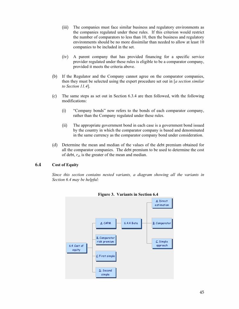
45
(iii) The companies must face similar business and regulatory environments as the companies regulated under these rules. If this criterion would restrict the number of comparators to less than 10, then the business and regulatory environments should be no more dissimilar than needed to allow at least 10 companies to be included in the set.
(iv) A parent company that has provided financing for a specific service provider regulated under these rules is eligible to be a comparator company, provided it meets the criteria above.
(b) If the Regulator and the Company cannot agree on the comparator companies, then they must be selected using the expert procedure set out in [a section similar to Section 11.4].
(c) The same steps as set out in Section 6.3.4 are then followed, with the following modifications:
(i) “Company bonds” now refers to the bonds of each comparator company, rather than the Company regulated under these rules.
(ii) The appropriate government bond in each case is a government bond issued by the country in which the comparator company is based and denominated in the same currency as the comparator company bond under consideration.
(d) Determine the mean and median of the values of the debt premium obtained for all the comparator companies. The debt premium to be used to determine the cost of debt, rd, is the greater of the mean and median.
6.4 Cost of Equity
Since this section contains nested variants, a diagram showing all the variants in Section 6.4 may be helpful:
Figure 3. Variants in Section 6.4
6.4 Cost ofequity
A. CAPM
B. Comparatorrisk premium
C. First simple
6.4.4 Beta
A. Directestimation
B. Comparator
C. Simpleapproach
D. Secondsimple

46
Section 6.4, Variant A: CAPM approach
Variant A gives the classic, full capital asset pricing model (CAPM) method.
6.4.1 The real cost of equity, re, is equal to: rf + (beta x MRP), where “MRP” means market risk premium.
6.4.2 The market risk premium (MRP) is determined as follows:
(a) Calculate the mean of the estimates of MRP made by the following regulators: [specify names]. For each regulator, the final determination from the latest [water utility] price review should be used. If a regulator has quoted a range and not a single-point estimate, the midpoint of the range is to be used for that regulator. The value obtained is the MRP to be used.
The names of the comparator regulators would be written in the rules. Only regulators that have undertaken at least one previous price review which has been perceived as being best practice, or close to it, with respect to the financial aspects of regulation should be included. Use a minimum of three names. Regulators that cover water utilities are to be preferred. Good candidates (including some regulators that do not cover water utilities) would be: OFWAT (England & Wales), ESC (Victoria), NER (South Africa), and SSIS (Chile).
(b) If a regulator specified in paragraph (a) ceases to exist, no longer determines the MRP, [or stops covering water utilities], then, if the Regulator and the Company cannot agree on a replacement for that regulator, the replacement must be determined by the expert procedure set out in [a section similar to Section 11.4].
6.4.3 [VARIANT: this section could be included in addition to Section 6.4.2.] After a value for MRP has been determined under Section 6.4.2, if either the Company or the Regulator believes that this estimate of MRP is too low, it is entitled to request that an independent financial expert carry out a determination under the procedure set out in Section 11.3. The expert determination will be carried out as follows:
(a) The expert will examine reports and other information from reputable regulators in the [region where the country is located], reputable investment analysts, and reputable academics, and will submit his best estimate of the MRP based solely on these secondary sources, in the light of his appreciation of the soundness of their analyses and their reputations (the weighting given to the conclusions of each source to be explained in the expert’s report).
(b) If the value submitted by the expert is greater than the MRP as determined in Section 6.4.2, then the MRP to be used is determined by taking a weighted average that gives a weight of one-third to the value submitted by the expert and a weight of two-thirds to the value as determined under Section 6.4.2. If the value submitted by the expert is less than the MRP as determined in Section 6.4.2, then the MRP to be used is the value as determined under Section 6.4.2.
The weights have been arbitrarily fixed in a ratio of 1:2. Other values could be used in the rules.
The adjustment in variant Section 6.4.3 is asymmetrical because it is designed to respond to a concern that some regulators under political pressure tend to bias their

47
estimates of the MRP downwards. One could, of course, revise the wording to make the adjustment mechanism work in either direction.
6.4.4 The value of beta is obtained in the following manner.
Section 6.4.4, Variant A: Direct Estimation of Beta
Variant A gives the classic, full method.
(a) Daily returns information are calculated for the Company equity and the [specified market index] over the past three years. All holidays must be removed. Dividend data are ignored.
(b) The equity beta is then calculated using ordinary least squares as:
mei rr βα += ,
where ri is the Company return and rm is the market index return. An estimated, i.e., non-zero, α must be imposed in the regression equation calculation.
(c) The standard error for βe is calculated. If there is a significant difference from both 1 and 0 at the 95 percent confidence level, this is the value to be used for beta. If there is no significant difference from either 1 or 0 at the 95 percent confidence level, then [either Variant B or C must be used instead—this means that one of these variants should be selected and written into the rules even if Variant A is selected as the primary method].
Explanatory Note. Variant A should be used only if there are at least three years of share price data and either sufficient liquidity (e.g., turnover) to ensure that prices are meaningful or the existence of a market maker system (where prices are updated even if no trade). Any period of market support at the time of privatization should be excluded.
In the Guidelines, this approach is considered to be a variant. If the Company were to float during the life of the PSP arrangement, a switch from one rule to another (after three years of good share price data) would certainly make sense. Instead of treating the rules as variants, one could envisage an automatic switching rule, but it is likely that both sides would agree on this when the time came. So a switching rule could be used based on agreement by both sides to shift to the method in Variant A.
The market index to be used should be specified in the rules (Section 6.4.4(a)). This would normally be the standard market index. If the sector or company accounts for more than 10 percent of the market value of the index, then an alternative broader index is needed. If no broader index is available for the country, then a regional index should be used in addition to the local index. If the values derived from the local index and the regional index diverge significantly (by more than 10 percent), then the comparator approach (Variant B) should be used instead.
Holidays should be known. A simple test is to see if there are days on which the index return is zero. If the company also has a zero return that day, it should be checked to establish whether this was a holiday.

48
One could also calculate an estimate of the equity beta for an industry rather than the Company; in that case, the same process should be followed except that an industry index should be used for the “company” return rather than the individual company figures.
Section 6.4.4, Variant B: Comparator Method for Estimating Beta
Variant B makes use of determinations that regulators in other countries have made.
(d) Selection of comparator companies or industries
Either (i) or (ii), below, would be used in the rules, not both. The only difference is that in (ii), the rules start out with a pre-established list of comparators that will be used for each price review unless a comparator has to be dropped from the list.
(i) [VARIANT] At each periodic review, appropriate comparators are chosen. These are between five and 10 comparator industries or companies facing similar regulatory and business risks to the one being regulated. Preference is to be given to countries where at least some of the companies are listed. If the Regulator and the Company cannot agree on the comparators, they must be selected by the expert procedure set out in [a section similar to Section 11.4].
Different comparators might be chosen at each price review since some companies may be taken over, new companies may be listed, and the regulatory regime in a country may change.
(ii) [VARIANT]
(A) The following industries or companies are to be used as comparators: [specify the names of between five and 10].
Countries or companies that could be included are: England & Wales water and sewerage (industry), Victoria water and sewerage in Australia (industry – if considered applicable), Philippines (Manila Water Company is now quoted), and Thailand (East water company is quoted).
(B) If a comparator in the list in paragraph (A) must be dropped and the Regulator and the Company cannot agree on a replacement comparator, it must be selected by the expert procedure set out in Section 11.4.
(C) A comparator must be dropped from the list given in paragraph (A) in the following circumstances:
(1) the comparator company has ceased to exist—e.g., it has been taken over by another company; or
(2) the comparator industry or company no longer faces similar regulatory and business risks to the one being regulated; or

49
(3) all regulated Companies and the Regulator agree to drop the name from the list.
(e) The value of beta to be used is determined by the following steps:
(i) For each comparator, take the last regulatory price determination and select the equity beta as determined by the regulator, either for the industry (where the regulator takes an industry approach), or the specific company (where that approach is followed).
(ii) Estimate the asset beta, βa, for each comparator company or sector by de-gearing the comparator’s equity beta by using the following formula:
( )comparatorcomparatorea g−×= 1,ββ
(iii) For each value of the asset beta, the adjusted comparator equity beta, βe, is estimated using the gearing of the Company or industry subject to the price review:
( )ga
e −= 1ββ
(iv) The mean of this set of equity beta values is taken. This is the beta to be used.
Section 6.4.4, Variant C: Simple Approach for Estimating Beta
This approach assumes that the asset beta (βa) of the Company is standard for the economy. The de-gearing formula is: βa = βe x (1 – g). So, since by definition βe = 1 for the economy, βa = 1 – gAll.
(f) Estimate the standard asset beta for the entire economy, βa, in the following manner. Take the average gearing for all quoted companies (gAll) and de-gear an equity beta of 1 using the following formula: βa = 1 – gAll.
(g) The average gearing for all quoted companies (gAll) is calculated on the basis of net debt as defined in Section 6.5.2. and the market value of equity.
(h) If it is not feasible to undertake a reliable calculation of gAll from original data, a credible secondary source (e.g., International Monetary Fund, reputable development bank, national statistics office) must be used to obtain a value for gAll. If a reliable value for gAll cannot be obtained in this manner, then a simplifying assumption of an equity beta of 1 for the Company or sector should be used and the step set out in paragraph (i) will be skipped. If the Company contests any aspect of the decisions made by the Regulator under this paragraph (h), the Company may invoke the expert determination procedure under Section [10.2] to resolve the issue.
(i) The equity beta to be used is determined using βa from paragraph (f) and the gearing of the Company (g) as follows:

50
( )gWACC a−= 1equation in used be toBeta β .
Section 6.4, Variant B: CAPM Approach with Combined Beta and MRP, Based on Comparators
This variant (for which the rules are not shown) would combine the comparator method used in Section 6.4, Variant A, to estimate the MRP and the comparator method of Section 6.4.4, Variant B, to estimate beta. The key point is that the estimation of both values would then be consolidated. Both values would be obtained from each comparator and then a sector-specific risk premium would be calculated for each comparator by multiplying the estimate of MRP and the estimate of (degeared) beta. Averaging would then be carried out using the estimates for the sector-specific risk premium. This is a simplified method that ensures consistency between the comparator estimates for MRP and for beta.
Section 6.4, Variant C: First Simple Approach
This variant must be used only in conjunction with the comparative or optimal gearing approach (Section 6.5.3, Variant C or D).
6.4.5 The real cost of equity, re, to be used is equal to the sum of a reference interest rate value and a stipulated equity premium.
6.4.6 The reference interest rate value equals the mean of the daily values of [specified reference rate—see the Explanatory Notes to the Guidelines] during the past six months, adjusted for [home country] inflation using the Fisher equation and:
(a) [VARIANT] last year’s annual inflation.
(b) [VARIANT] a weighted average of annual inflation figures for the past three years, where the weights are 0.5, 0.3, and 0.2, beginning with the most recent past year.
The second variant is included simply to show that some smoothing could be used if there is a worry that one single year’s figure may not be a good reflection of market expectations about the future. The particular smoothing formula adopted need not be the simple one given here.
6.4.7 The equity premium equals […] percent.
The value used must be consistent with the comparator or optimal gearing approach (Variant C or D of Section 6.5.3).
Explanatory Note. This variant uses a country-specific reference interest rate to allow flexibility to respond to changes in macro-economic conditions. But the equity premium is fixed (there is no beta and no MRP); this ensures that investors know exactly how much additional return they are allowed—not dissimilar to some of the Latin American approaches but a little more flexible—possibly closer to the Chilean water approach.
The reference interest rate (Section 6.4.6) would be specified in the rules. It would be the country-specific equivalent of LIBOR or EURIBOR—i.e., it must capture the country premium. For example, in Pakistan this would be KIBOR, the Karachi Inter-Bank Offered Rate. If there is no country-specific reference interest rate, then Variant C should be used.

51
This value of the equity premium (Section 6.4.7) would be fixed in the rules in absolute terms and could be modified only through whatever procedure has been adopted in general for modifications of the regulatory rules. (See the Explanatory Notes to the Guidelines.) The fixed equity premium should be determined through a consideration of the returns necessary in other similar countries or sectors to attract equity finance, based on advice from an internationally respected financial consultant. Section 6.4, Variant D: Second Simple Approach
This variant must be used only in conjunction with the comparative or optimal gearing approach (Section 6.5.3, Variant C or D).
6.4.8 The real cost of equity, re, to be used is equal to the sum of a risk-free rate and a stipulated equity premium.
6.4.9 The risk-free rate, rf, is determined in accordance with Section 6.2. Use one of the three variants for that section.
6.4.10 The equity premium equals […] percent. This is to be fixed in the rules. See Explanatory Note for Variant B.
The value used must be consistent with the comparator or optimal gearing approach (Variant C or D of Section 6.5.3).
6.5 Gearing
6.5.1 Gearing, g, is defined as:
BaseAsset RegulatoryDebtNet =g ,
where RAB is defined in Chapter 4.
6.5.2 Net debt, for the regulated activity, is defined as the sum of:
(a) Net short-term borrowing (short-term borrowing minus cash in hand and bank)
(b) Net long-term borrowing (long-term borrowing minus financial investments)
(c) Leases (finance leases only)
(d) Net trade creditors (trade creditors minus trade debtors)
(e) Net other (other liabilities minus other receivables)
Accounting terms should reflect local terminology if it differs from the United Kingdom's terminology used here.
6.5.3 The value of g to be used in the WACC equation is determined as follows.
Section 6.5.3, Variant A: Actual Gearing – Individual Company Approach

52
(a) Calculate the mean of the forecast gearing of the Company over the next price control period, averaging yearly values, based on projections of net debt and RAB established as part of the price review process. This is the value of g to be used in the WACC equation for the Company.
Care should be taken to ensure that the financial viability rules relating to gearing are adhered to in approving the inputs that enter into the forecasts. See Section 2.5.
Section 6.5.3, Variant B: Actual Gearing – Sector Approach
(b) Calculate the mean of the forecast gearing of the Company over the next price control period averaging yearly values (“Company forecast gearing”), for each Company in the industry based on projections of net debt and RAB established as part of the price review process.
Care should be taken to ensure that the financial viability rules relating to gearing are adhered to in approving the inputs that enter into the forecasts. See Section 2.5.
(c) The value of g to be used in the WACC equation is the mean of all the Company forecast gearings, subject to paragraphs (d), (e), and (f).
(d) If a Company forecast gearing is greater or less than the value determined in paragraph (c) by at least [10] percentage points, then the Regulator must allow the Company a value of g which is [10] percentage points greater or less (respectively) than the value determined in paragraph (c).
(e) If (i) a Company forecast gearing is greater or less than the value determined in paragraph (c) by more than [5] percentage points and (ii) the divergence in forecast gearing is justified because of special features of the Company or special circumstances faced by the Company and is consistent with a sound capital structure for the Company, then the Company forecast gearing must be used in the WACC equation for that Company.
(f) If the Company believes that conditions (i) and (ii) in paragraph (e) are satisfied but the Regulator disagrees, the Company may invoke the expert determination procedure under Section 11.2 to determine the issues in paragraph (e).
Section 6.5.3, Variant C: Actual Gearing – Comparator Approach
(g) The following companies are to be used as comparators: [specify between 5 and 10 names; the names would be written into the rules].
(h) A new comparator will be added to the list:
(i) if a comparator in the list in paragraph (g) must be dropped;
(ii) if this is necessary so that at least one comparator is another regulated activity in the same country and at least two comparators are regulated water businesses in countries with similar economic conditions.

53
(i) A comparator must be dropped from the list given in paragraph (g) if it has ceased to exist (e.g., it has been taken over by another company) or if it is no longer a company:
(i) that faces similar regulatory and business risks to the one being regulated;
(ii) that faces tax rules similar to the rules faced by the regulated companies; and
(iii) that is at a similar stage of the investment cycle as the regulated companies.
(j) It the Regulator and the Company dispute whether the conditions in Section 6.5.3(h) or 6.5.3(i) are met, the matter may be referred by either the Regulator or the Company to expert determination under Section 11.2. If the Regulator and the Company cannot agree on the selection of a replacement comparator company, it must be selected by the expert procedure set out in [a section similar to Section 11.4].
(k) For each of the comparators, the level of gearing is calculated for each of the three latest years available. Calculate the mean for each comparator for three years of data. If data for fewer than three years are available, then the mean for that comparator is calculated over the longest time period for which data are available. If any of the comparators used are not regulated companies or are companies for which the regulator has not established a formal RAB, then the market value of equity plus the net book value of debt should be used in place of the RAB in the gearing formula.
(l) Calculate the mean of the mean values for the comparators. This is the value of g to be used in the WACC equation.
In addition, note that one could develop another, related variant that bases the optimal gearing on recent determinations by a set of regulators as to the optimal gearing of their regulated companies.
Section 6.5.3, Variant D: Optimal Gearing – Stipulated-value Approach
(m) The value of g to be used in the WACC equation is […] percent.
This is the simplest approach. A specific value is written into the regulatory rules. An internationally respected financial consultant should be engaged to recommend an optimal capital structure for the company. If conditions later change enough to call into question this value, then the rules would have to be modified using the normal procedure for rule modification.
Explanatory Note. There are three broad approaches for determining the gearing to be used in calculating the WACC: actual, comparator, or optimal. In principle, the optimal-gearing or comparator approaches (Variants D or C, respectively) are preferred. Using actual figures (with a preference for sector average—namely, Variant B), however, would seem at first glance to be more conducive to a low-discretion approach. But if an expert procedure (as in Chapter 11) can be used to select comparators, then the comparator approach of Variant C might be more feasible.

54
6.6 Embedded Debt
Section 6.6, Variant A: One-off Adjustment
6.6.1 This Section 6.6 applies only to fixed-rate debt (including floating rate debt swapped to fixed) existing at the time the regulatory regime enters into effect (“embedded debt”). This is a one-off adjustment and once made, no further changes to the embedded debt are reflected in the RAB.
N.B. The following adjustments should be made only if, for some reason, an adjustment has not already occurred through the bidding or negotiation process by which the PSP arrangement was established. If bidders know in advance how the initial RAB and cost of debt will be determined, then they will take into account in their bid price the cost of embedded debt. Advisors should carefully examine the conditions under which the PSP arrangement will be established and should delete or modify these provision if appropriate. (Note that these guidelines do not apply to situations in which a new regulatory regime is being applied to an existing PSP arrangement.)
6.6.2 The following adjustment must be made if the cost of the embedded debt (red) is different by at least [2] percentage points from the cost of debt as determined under Section 6.3 (rd).
(a) Calculate the following value:
⎟⎟⎠
⎞⎜⎜⎝
⎛−×
d
ed
rr1 debt embedded of valuegOutstandin
(b) Subtract this value from the RAB as determined in Chapter 4. Use this adjusted RAB value in place of the RAB as determined in Chapter 4.
Section 6.6, Variant B: Periodic Cash Flow Adjustment for High-cost Embedded Debt
6.6.3 This Section 6.6 applies only to fixed-rate debt (including floating rate debt swapped to fixed) existing at the time the regulatory regime enters into effect (“embedded debt”).
This adjustment method could be used if the cost of the embedded debt (red) is expected to remain greater than the cost of debt as determined under Section 6.3 (rd).
6.6.4 An adjustment at each price review is made, as follows:
(a) The Company provides an audited estimate of interest payments (and related fees [see Section 6.1.3]) on embedded debt that will be due over the forthcoming control period.
(b) The Regulator determines what the interest payments (and related fees) would be assuming the cost of debt as determined under Section 6.3 and assuming the same principal repayments year by year as in paragraph (a).
(c) The annual cash flows in paragraph (b) are subtracted from the annual cash flows in paragraph (a). The resulting values are added to the corresponding annual revenue requirements for the forthcoming control period (before discounting).

55
(d) This adjustment is carried out at every price review until the embedded debt has been entirely repaid.
Explanatory Note. There are circumstances in which governments have not been willing to restructure existing debt prior to private sector participation. This debt may be either cheap (such as IFI and bilateral concessional lending) or expensive (some government onlending) relative to existing market rates. Rather than leaving an ongoing problem for the regulator, it is better to make a one-off adjustment to the RAB so that market rates can be used in the future.
Variant B is provided as a method that could be used in some circumstances when the cost of the embedded debt is above market rates. Rather than increase the RAB, it is possible to allow a cash-flow adjustment at every price review. Note that this method is proposed only for circumstances in which red > rd, and not where red < rd. The reason is that we should be especially concerned to avoid driving the Company into financial distress because of debt terms that it inherited when the PSP arrangement started. In some cases, we may be worried that a one-off adjustment, as in Variant A, might still leave too much downside risk if interest rates were to fall.
The Guidelines do not try to assess whether incurring prepayment fees and then refinancing is a cheaper alternative. The company has an incentive to achieve this since it would keep any benefit for the rest of the price control period. Assessing the cost of prepayment, etc., could drag the regulator into micromanagement and having to assess the real depth of the local market for handling such debt. 6.7 [VARIANT] Adjustment for Downwards Interest Rate Shock
This is a variant that could be included if there is a worry about large drops in interest rates where refinancing is difficult. See Explanatory Note.
6.7.1 The following adjustment must be made at a price review if the cost of any existing debt is greater than the cost of debt as determined under Section 6.3 by at least [5] percentage points and the Company can demonstrate that the terms of the existing debt were prudently contracted when the borrowing occurred and (where these rates are known) were in line with comparable market rates at that time.
(a) The Company provides an audited estimate of interest payments (and related fees [see Section 6.1.3]) on the relevant existing debt that will be due over the forthcoming control period.
(b) The Regulator determines what the interest payments (and related fees) would be assuming the cost of debt as determined under Section 6.3 and assuming the same principal repayments year-by-year as in paragraph (a).
(c) The annual cash flows in paragraph (b) are subtracted from the annual cash flows in paragraph (a). The resulting values are added to the corresponding annual revenue requirements for the forthcoming control period (before discounting).
(d) Period of applicability:
(i) [VARIANT] This adjustment is carried out at every price review so long as the cost of the relevant existing debt is greater than the cost of debt as determined under Section 6.3 by at least [5] percentage points and until the existing debt has been entirely repaid.

56
(ii) [VARIANT] This adjustment is carried out at the following […] price reviews [specify how many future price reviews] and only so long as the cost of the relevant existing debt is greater than the cost of debt as determined under Section 6.3 by at least [5] percentage points.
Explanatory Note. There might be circumstances in which a downside interest rate shock will reduce forward looking rates substantially below historic rates. In these circumstances the cash flows of the company may be insufficient if the cost of debt is determined on a forward-looking basis. An adjustment could be made as under Variant B of Section 6.6 to protect the financial viability of the company.
A variant is also provided in paragraph (d) that limits the period over which this protection is provided so as to incentivize the company to refinance existing debt and ensure as quick a pay-down of existing debt as possible. The length of time allowed for the company to achieve this will obviously depend on the depth of the capital markets, the future borrowing needs for new capex, and the cost of refinancing the existing debt (including any early-repayment fees). Consequently detailed consideration to these issues should be undertaken before setting the value. 6.8 [VARIANT] Debt As a Cost Pass-through
This approach is a variant that could be used in place of Section 6.3. The approach could be used if data on the cost of debt are hard to collect (or forecast) or if the law requires such an approach to be followed.
This section is not located as a variant within Section 6.3, however, because it falls outside the WACC approach referred to in Section 6.1. Using this approach would replace all the sections of this chapter except Section 6.4.
These guidelines have not been developed to the same degree as the rest of this chapter—especially regarding internal group debt.
6.8.1 The cost of capital will be accounted for by two sets of annual values to be added to the annual revenue requirements (before discounting) for the forthcoming control period: one set of annual values relating to equity and one set relating to debt.
6.8.2 The annual values relating to equity are determined by multiplying the cost of equity (re), as determined under Section 6.4, by the forecast value of equity in each year, which is deemed to be equal to the RAB minus net debt.
This is equivalent to using the WACC equation to determine the annual revenue requirements in the standard way but while setting rd = 0.
6.8.3 The cost of debt is accounted for in the following way, subject to Section 6.8.4:
(a) Interest payments are estimated for the price control period based on debt agreement terms and existing interest rates (and taking into consideration any swaps and similar financing instruments) and forecast levels of debt. These values are included in the annual revenue requirements under Chapter 2.
57
(b) During the control period, allowed revenue in any year relating to the cost of debt is based on the forecast for that year plus a correction from the previous year to compensate for any under- or over-forecast of interest in that year.
More precision will be needed for this provision. The correction mechanism is the same as for pass-through opex items. See Chapter 3.
6.8.4 Sections 6.8.3(a) and 6.8.3(b) are subject to the following prudency test.
(a) If the forecast interest rate or the rate actually paid is greater than [1 + …] times [a standard market interest rate—e.g., prime lending rate or some other commonly quoted and transparent business borrowing rate] then the Company must provide documentary evidence to the regulator demonstrating that the rate forecast to be paid or actually paid is prudent. If the prudent rate is determined to be less than the rate that would otherwise be used in the forecast or correction, then the prudent rate will be used instead.
(b) [VARIANT addition to (a)] The forecast or actual rates (as the case may be) will be deemed to be prudent if the documentation provided by the Company includes quotes from at least three major reputable banks and shows that the most advantageous quote (given the conditions imposed on the borrowing) was accepted.
Explanatory Note. Handling debt as a cost pass-through simplifies the cost of capital calculation but removes the incentive for the company to borrow as cheaply as possible. While two ways in which this incentive can be partly reintroduced are noted above, it must be accepted that this will be inferior to the WACC-based approach. 6.8.5 Any internal group debt (debt from a closely related company) must be:
(a) [VARIANT] treated as equity for purposes of both the gearing and cost of equity calculations.
(b) [VARIANT] treated as a mixture of debt and equity according to [a specified optimal gearing calculation]. If any of the internal group debt is thereby treated as debt it will carry the same interest rate as the average of all the external debt of the Company.
(c) [VARIANT] treated as debt but subject to a cap on the interest rate fixed at the average interest rate on all the external debt of the Company.
Explanatory Note. Internal group debt is often a major source of finance for a company, especially during the start-up phase. However, it is often treated more as equity in terms of rates, priority of repayment, subordination to external senior lenders, etc., and is as much a way for the parent company to extract value as it is for providing finance. Consequently this needs to be handled very carefully by regulators to ensure that an appropriate return is being allowed. The three variants offered above are not the only possibilities; rather they are designed to show the possible types of approach that could be adopted.

58
Chapter 7. CAPITAL MAINTENANCE CHARGE 7.1 General
7.1.1 The provisions of this Chapter 7 describe how to determine the capital maintenance charges that are to be included in the annual revenue requirements under Chapter 2.
7.1.2 The capital maintenance charge for a specific year is the sum of the network renewals charge (NRC) (see Section 7.2) and the depreciation charges (see Section 7.3).
Note that “depreciation charge” as used in this chapter has no necessary relation to the depreciation charge used in the conventional financial statements or for profit tax purposes.
7.1.3 The capital maintenance charge applies to all assets which the company has the responsibility to maintain and replace, including those assets initially funded by customer or government contributions.
The application of a capital maintenance charge to assets funded by customer contributions is a controversial issue. Utilities may argue that it is necessary for the financing of the replacement of these assets at some point in the future, but customers may be concerned that they are asked to pay for the same asset twice. Even if one does not agree with the rule given above, the following points are uncontroversial:
• Customer funded assets should not be included in the regulatory asset base. • If a capital maintenance charge for customer funded assets is included in the
build-up of regulated prices, this charge should be deducted from the regulatory asset base, even though it excludes the customer funded assets. This is equivalent in NPV terms to not including capital maintenance charges for customer funded assets but achieves a different profile of charges over time.
This issue is discussed further in the Explanatory Notes to the Guidelines.
7.2 Network Renewal Charge
7.2.1 The network renewals charge is defined (for purposes of determining its value) as the best estimate of the average annual capex over the next [15] years that would be needed, assuming that the underground assets are currently in a condition capable of delivering the required levels of service, to maintain these assets so that they could continue to deliver the required levels of service on a sustainable basis.
If currently required service standards are far from minimum reasonable service standards for water and wastewater systems, one could specify a date in the future or specify a set of target service standards instead of referring to the “required levels of service.”

59
Explanatory Note. The concept of an NRC is based on the idea that for underground water and wastewater networks, it is much more sensible and practical for engineers to estimate the average amount of repair and renewals work that will be needed by developing a strategic plan for the specific works that need to be carried out during a given period into the future to maintain service levels, rather than to arrive at the figure by first adding up conventional depreciation values for all the asset categories, based on the (often arbitrary) useful life of the assets in each category, and then making any needed adjustments based on other factors to take into account actual asset condition and the risk of service deterioration. In effect, the NRC could be viewed as a kind of total-network-system depreciation, arrived at more holistically, rather than piece-by-piece.
The infrastructure renewals concept is often based on existing service levels. The major difference between how the concept would be used in a typical developing country context and how it is used in, say, England & Wales is that in a developing-country context, present levels of service may be far below the levels that should be used as a reference point for estimating the NRC. This makes the estimation more hypothetical and difficult, to be sure. But it is still important to make the estimate.
Specifying the value of NRC determines who funds this amount of network capex. The definition above entrenches in the rules the idea that customers must pay this (or an external source of subsidies must be found); in other words, the company cannot be asked to finance the basic level of capex that would be needed just to maintain serviceability—and hence the economic value—of the networks.
Note that estimating the NRC value would not necessarily affect the way the investment plan is developed or presented when there is a great deal of backlog work to be done: it would generally not make sense to identify certain works or assets as relating to backlog capex or relating to network renewals expenditure (pipes have to be replaced in either case). The NRC value, taken alone, is somewhat hypothetical in nature until most of the backlog capex has been dealt with. Moreover, the optimal amount of network renewals during a particular control period may not be simply five times the NRC; the optimal expenditure profile may not be constant over the horizon of 15 to 20 years. 7.2.2 Related definitions are as follows:
(a) “Backlog capex” means capex required for the existing network to bring levels of service up to the required levels.
(b) “Forecast network capex” means the estimate, made at business plan stage, of the network rehabilitation and renewals expenditure planned for a specified period, including any backlog capex.
(c) “Actual network capex” means the amount actually expended by the Company on network rehabilitation and renewals during a specified period, including any backlog capex.
(d) “Actual network renewals expenditure” (“actual NRE”) means the amount actually expended by the Company on network renewals during a specified period once levels of service have reached the required levels (i.e., once backlog has been dealt with).

60
Until backlog capex is dealt with, it would make little sense over the short- or medium-term to try to separate out renewals expenditure in the strict sense, i.e., excluding backlog capex.
7.2.3 The initial network renewals charge is determined as follows:
Section 7.2.3, Variant A: Good Information About the Networks Exists
(a) The unindexed (annual) network renewals charge is set at […].
Section 7.2.3, Variant B: Much Backlog Network Capex To Do Or Poor Information About the Condition Of the Network
(b) The unindexed (annual) network renewals charge is set at […].
There may be a need to allow for a simple update (using the same methodology) at the first price review if the full study has not been undertaken by that time.
(c) No earlier than […] and no later than […], a study will be carried out, as set out in Section 7.2.5, to update the network renewals charge.
The dates will have been specified based on the initial assessment of asset condition and information undertaken before the PSP arrangement begins. Depending on the state of the networks, the new study might take place during the first or second control period.
Explanatory Note. If there is reasonably good information about the networks when the PSP arrangement begins (which may be possible only after a considerable progress have been made in reducing the backlog of network capex), then a full study should be carried out before the start of the PSP arrangement to determine the initial network renewals charge (in accordance with the definition given in Section 7.2.1). The study should be made available to bidders and the public and sufficient discussion should take place to ensure that all relevant information has been taken into account.
If, at the start of the PSP arrangement, initial information about the condition of network assets is poor or much backlog capex needs to be done, it may not be realistic to undertake a sufficiently extensive study before private involvement, and so there may need to be a two-stage process. Before private involvement begins, a best estimate of the network renewals charge would be determined as part of the general pre-bid preparatory studies on asset condition, etc. This would admittedly be a very rough value. The information would be updated as soon as better information is available.
If there is a great deal of backlog to do at the start of the PSP arrangement, engineers might find it uncomfortably speculative to conduct the study to determine the NRC value as defined in Section 7.2.1, since the major assumption (that network assets are currently in a condition capable of delivering the required levels of service) might be far from reality. In that case, the terms of reference for the preliminary study could instead instruct the engineers to roughly estimate the steady-state NRC—i.e., based a rough MEA value of the network and rough but realistic asset lives. This would serve the purpose of fixing an initial value for how much network renewals expenditure should be included in customer tariffs on a pay-as-you-go basis.

61
7.2.4 A new study will be carried out, as set out in Section 7.2.5, to update the network renewals charge under any of the following conditions:
(a) If at the end of a control period, the current NRC will have been in effect for two control periods, and either the Regulator or the Company wishes a new study to be carried out. In that case, the study will be carried out in the last year of the control period and the results must be available sufficiently in advance of the price review.
(b) If at any time, levels of service relating to the network fall significantly below the required levels and either the Regulator or the Company wishes a new study to be carried out.
“Significantly” would need to be further specified; it might include some notion of a persisting deficiency in service levels as well as quantum thresholds.
(c) During the last year of any control period, provided that the Company wishes this and the Company bears the entire cost of the study (in that the cost would not be included in allowed revenue, as it would be for the other cases).
(d) If cumulative actual network capex since the current NRC value came into effect (based on an NRC study) is less than [75] percent of the cumulative NRC over that period and the Regulator wishes a new study to be carried out.
The purpose of the conditions above is to prevent an updating of the NRC from taking place automatically at every price review and hence to encourage greater stability of the NRC value for purposes of stabilizing tariffs. Paragraph (c) gives the Company an additional way to have a new study carried out and paragraph (d) gives the Regulator an additional way.
7.2.5 Any study undertaken under this Section 7.2.5 to determine or update the network renewals charge must comply with the following requirements.
(a) The NRC must be determined based on the definition given in Section 7.2.1.
(b) The study will be carried out in the following manner:
(i) [VARIANT] Terms of reference are agreed between the Regulator and the Company, a study is carried out by an independent consulting firm hired by the Company, with the report made public, and then if the Regulator and the Company cannot agree the NRC value, the Company is entitled to have the issue decided by expert determination under Section 11.2.
(ii) [VARIANT] The entire study, from the start, will be treated as an expert determination under Section 11.3.
(c) The study must:
(i) include a comparison of actual NRE and forecast NRC over at least the previous five years;
(ii) assess the impact on service levels, the optimality of any opex trade-off, the actual investment options available (e.g., deferring rehabilitation for a few

62
years since a major replacement will occur as part of a planned network expansion), and the implementation capacity of the company or sector; and
(iii) provide an opportunity for the company to justify any divergence.
More should be said in the rules about the nature of the study and the role of the company and regulator—e.g., concerning the opportunity to comment. The results of the study should be made public.
7.2.6 The NRC value, as updated under Section 7.2.5, will apply starting with the next control period.
The NRC is like depreciation (rather than opex) in that it is amenable to NPV-neutral revenue smoothing over more than one control period to mitigate any tariff shocks caused by jumps in its value.
7.2.7 The network renewals charge to be included in the revenue requirement under Chapter 2 is the unindexed NRC adjusted to the date of the price review by indexation to the [appropriate reliable price index—ideally one used for similar kinds of works such as a construction price index].
7.2.8 Until the first control period in which there is no further backlog capex forecast to be implemented:
(a) any excess of forecast network capex over the NRC will be treated as forecast capex for purposes of Chapter 8; and
(b) any excess of actual network capex over the NRC will be treated as actual capex for purposes of Chapter 8.
The effect of this section is that, during this period, any discrepancy between forecast and actual is dealt by the regulatory rules in the chapter on capex and not as a network renewals provision, as in the next section. This reflects the difficulty of distinguishing what is true renewals expenditure as long as there is backlog to deal with. The result is that actual NRE is deemed to be equal to NRC during this period.
7.2.9 Beginning with the first control period in which there is no further backlog capex to be implemented, if in any year actual NRE is different from the NRC, the difference must be reflected in the regulatory accounts as a provision and will be subject to standard audit requirements.
The rules would need to describe this in more detail. In effect, the cumulative balance of the difference between actual NRE and NRC is treated as either an asset or liability, as the case may be, in the regulatory books.
7.2.10 Whenever a new study is carried out under Section 7.2.5 to update the NRC, the cumulative network renewals provision in the regulatory accounts (positive or negative), if any, will be reduced to zero and a corresponding adjustment included in the revenue requirement for the next control period.
The adjustment for any change is designed to ensure no big swings in tariffs as a result. If a positive provision has been established—i.e., the old NRC was higher than actual NRE—then prices will be reduced during the next price control period. NPV-neutral smoothing would be achieved by using the WACC.

63
7.3 Depreciation of Above-ground Assets
7.3.1 The annual depreciation charge for all above-ground assets existing at [the date when the PSP arrangement and the regulatory regime started] is set at [amount] in unindexed terms. This value may not be revised.
Explanatory Note. The depreciation charge relating to existing above-ground assets will be set before the regulatory regime takes effect. It is not adjusted after that (there is no periodic revaluation), except for indexation under Section 7.3.6. This reduces risk for the company. The charge relating to existing assets can be set in one of two ways.
The first method for setting this part of the depreciation charge is to base it on the results of an optimized MEA valuation of the existing above-ground assets carried out before the PSP arrangement begins. This may well be a rough-and-ready study, given the lack of available information. It is important that appropriate constraints are imposed on the optimization so that a realistic value is determined. Two key constraints will be the demand characteristics and the configuration of the underground assets (which are excluded from the MEA study).
An average remaining asset life would be determined as part of the MEA study (see Section 7.3.3—the same criteria should apply). The depreciation charge would be determined by depreciating the MEA value over the average remaining life using straight-line depreciation.
The second method is to base the depreciation charge on the initial value for the RAB, which has been determined as discussed in Chapter 4. In the simplest version of this method, one would assume that the underground assets have no value in terms of the initial RAB (this would certainly make sense if the initial value of the RAB is clearly lower than a rough guesstimate of the MEA value of the above-ground assets). Otherwise, one would need to allocate the RAB between depreciable above-ground assets and the underground assets subject to the network renewals charge. If the simple version is followed, one would then estimate an average remaining asset life through a rough asset condition assessment. The initial RAB would be depreciated over this average remaining asset life, using straight-line depreciation. 7.3.2 The unindexed depreciation charge for an asset added to the above-ground assets is
determined by dividing its investment cost by its asset life (straight-line method). For this purpose, “investment cost” refers to forecast or actual values, as the case may be, in accordance with the provisions of Chapter 8.
7.3.3 The asset life applicable to a specific asset or asset category must meet the following conditions:
(a) It must be based on commercial life. For this purpose, commercial life means the period over which the asset will be used to deliver services ending when the NPV of expected future whole-life costs (operation, maintenance, repairs, rehabilitation, and replacement) assuming immediate replacement is less than the NPV of expected future whole-life costs assuming replacement at a later time.
The term “commercial life” and not “economic life” has been used here because some people use “economic life” in a way that takes into account the benefit side also—future demand, obsolescence, etc. The aim is to exclude these more speculative aspects.
64
(b) To the extent not inconsistent with paragraph (a), it must use internationally accepted standards (including, if appropriate, manufacturers’ estimates), unless there is a specific justification for using a different value (e.g., the chemical composition of the surrounding soil and the aggressiveness of the water is likely to cause a certain type of pipe to corrode more rapidly).
7.3.4 The company must propose and justify asset lives relating to new assets in the business plan submitted for each price review. These must be verified by the company’s technical auditors.
“Technical auditor” will need to be defined elsewhere in the rules and the role of the Regulator in the appointment process specified.
7.3.5 The company may propose revisions to the remaining asset life of a specific asset or category of assets, justified under Section 7.3.3 and verified by the company’s technical auditors. Such a revision may be proposed only in the business plan submitted at the time of a price review. No revisions or retroactive adjustments will be made concerning asset lives relating to past depreciation.
7.3.6 The depreciation charges to be included in the revenue requirement under Chapter 2 are the unindexed depreciation charges adjusted to the date of the price review by indexation to the CPI.
7.3.7 Whenever the RAB is adjusted under Section 8.3 to take into account actual capex relating to an asset, the future depreciation charge for the relevant asset will be adjusted in the following manner:
(a) first, add the difference (positive or negative) between allowed actual capex and previously forecast capex to the remaining forecast value of the asset (i.e., after depreciation of forecast value);
(b) then calculate depreciation of the resulting value over the unchanged remaining asset life on a straight-line basis.
7.4 Additional Guidelines Applicable to Limited-duration Concessions
7.4.1 Notwithstanding the provisions of Section 7.3, the remaining asset life for purposes of determining a depreciation charge must not be greater than the remaining number of years of the concession. This Section 7.4.1 does not apply, however, to depreciation of assets to the extent that they have been accounted for as customer or government contributions.
The accounting treatment should be based on a restatement of accounts adopted at the start of the period during which the regulatory regime has been in effect.
7.4.2 For any asset (or asset category) whose remaining asset life as determined under Section 7.3 is greater than the asset life as determined under Section 7.4.1, the regulatory accounts must show the depreciation charge broken down into two constituent values: the charge as it would be calculated under Section 7.3 (“normal depreciation charge”) and the difference between that charge and the charge as calculated under Section 7.4.1 (the difference being referred to as the “supplementary depreciation charge”).

65
This is important to ensure transparency and prevent confusion.
7.4.3 During the last [two] control periods before the end of the concession, unless the concessionaire agrees otherwise the concessionaire will not be required to finance capex to the extent that the supplementary depreciation charge relating to that capex would cause average tariffs to be at least […] percent greater in any of the remaining years of the concession than they would be if there were no supplementary depreciation charge.
Explanatory Note. Concessions with a limited duration pose additional problems for depreciation. (Once again, it should be noted that we are referring to regulatory depreciation. Depending on the country, the concessionaire may not be able to depreciate the assets it does not own in its financial accounts. Or in a francophone country, the concessionaire may be required to use the conventional accounting scheme designed for depreciation by concessionaires.)
The concessionaire must be allowed to recover its investments, but as the concession advances, there is less and less time over which to do this. The Guidelines present one way to deal with the issue. Another way would be to use normal depreciation in all cases and for the public authority to pay the concessionaire the remaining asset value at the end of the concession, but, as simple as this solution seems, it may not be acceptable to either the government or the concessionaire. The entire issue is discussed more fully in the Explanatory Notes to the Guidelines.
In keeping with typical practice for classic concessions, Section 7.4.1 assumes that there will be no remaining asset value at the end of the concession. A variant of this—certainly to be recommended if the terminal-payment risk is considered to be manageable— would allow for a remaining value up to a specified maximum, which would then be paid by the public authority to the concessionaire at the end of the concession. In this variant, normal depreciation would be used until the remaining value reached the ceiling. At that point, the regime as described in the section above would take effect. Political risk insurance or guarantees (breach of contract) could be considered by the concessionaire to mitigate the risk that the public authority will not pay the remaining asset value.
The purpose of Section 7.4.3 is to put a limit on how much additional capex can be packed into the final years of a concession, where it will have to be recovered over fewer and fewer years. Public authorities have several ways to deal with this constraint: they can try to convince the concessionaire to agree to higher tariff increases; they can postpone some of the new capex until the end of the concession; they can provide government funding for it; or they can try to negotiate with the concessionaire an increase in the amount of the terminal payment to be made by the public authority to the concessionaire.

66
Chapter 8. CAPITAL EXPENDITURES (CAPEX) Explanatory Note. This chapter focuses on how capital expenditures (capex) are treated in the price review and in later adjustments to the RAB. It does not deal with the process by which the Regulator communicates requirements to the company, the company prepares a business plan (possibly to be vetted by an independent expert engaged by the company), stakeholders are consulted, the Regulator scrutinizes the business plan, etc. These process aspects are extremely important, but they are not within the scope of the present Guidelines.
Also, the chapter does not deal with the required contents of the business plan, especially how capex should be disaggregated, categorized, and justified on the basis of asset condition and performance assessments, among other things. These aspects, however, are touched on in the Explanatory Notes to the Guidelines.
Standardization of information requirements (e.g., by the use of standard forms, templates, and computer files) is important as a way to increase predictability and efficient preparation and analysis—and to ensure comparability among different regulated companies. Regulators and designers of concession agreements can make use of a growing body of examples of such standardized documents, collected and proposed at an international level (see references in the Explanatory Notes to the Guidelines).
Given that different rules may apply to different categories of capex, it is most important that appropriate and precise accounting rules be set out in the regulatory rules to prevent gaming by shifting capex from one category to another (and from capex to opex and vice versa). This is discussed more fully in the Explanatory Notes to the Guidelines. 8.1 Notation, etc.
8.1.1 Notation for this chapter is as follows:
RAB Regulatory Asset Base
ABR Forecast RAB
nvI Forecast capex Inv Actual capex
epnD Depreciation as determined under Chapter 7
G Forecast government contributions
C Forecast customer contributions  Forecast asset sales
8.1.2 In this chapter, the current control period is sometimes referred to as “control period 0” (and is indexed by the subscript “0”), the forthcoming control period (i.e., the control period whose tariffs are the object of the present price review) as “control period 1”
67
(indexed by the subscript “1”), and the immediately following control period as “control period 2” (indexed by the subscript “2”), and so on. (See also Section 1.2.1.)
8.1.3 In this chapter, unless otherwise indicated, all cost- and revenue-related values are given in real terms. Indexation to the CPI must be carried out if and as appropriate.
More detailed rules should be provided for this in the actual regulatory rules. This task will be an obvious one to competent regulatory advisors.
8.2 Determining the Capex Program for the Forthcoming Control Period
As noted in the Explanatory Note above, the company makes the first move by submitting a business plan that contains a capex program, among other things. These aspects are not dealt with in the present Guidelines.
8.2.1 The capex program for the forthcoming control period must be a program:
(a) that is designed to achieve, in a reasonably efficient manner and in accordance with accepted good industry practice, the requirements communicated to the Company by the Regulator and any other requirements under law; and
(b) that, at a minimum, is designed so that there is no deterioration of the quality of service below existing levels.
Explanatory Note. The requirements communicated by the Regulator (some of them reflecting standards set by other agencies—e.g., water quality standards) are likely to consist of a mix of output requirements and input requirements or budget limits. For example, in many systems there is an enormous need to replace aging water mains. Given numerous kinds of uncertainty, it may be impossible to drive the amount of replacements for the forthcoming control period solely by setting output performance standards. So the requirements might be specified partly in terms of minimum and maximum limits for inputs (e.g., km of mains to be replaced). The particular way that requirements are best expressed for a given system at a given stage has to be worked out for each system. General guidance can be given, but not generic rules.
Paragraph (b) is intended to entrench in the rules a limit as to how low tariffs can go in response to affordability or political concerns. If at the time the rules are drafted, service quality is unnecessarily high on some dimensions (e.g., perhaps with respect to certain types of customers), paragraph (b) can be qualified in an appropriate way.
The following two sections are merely indicative and are not complete. System-specific advisors may wish to modify, add to, or delete these sections.
8.2.2 In determining whether a capex program meets the conditions in Section 8.2.1, the Regulator:
(a) must consider:
(i) whether the program is likely to support the target growth in customer connections and forecast overall demand growth;

68
(ii) whether each component of the program is justified in terms of how it contributes to meeting the requirements set for the Company, given what is known about the present condition of assets;
(iii) for each major asset that needs to be replaced, the trade-offs between proactive replacement versus reactive replacement (taking into consideration the cost of failure);
(iv) the cost implications of including any item in the capex program and the consequent impact on affordability; and
(v) [others, as needed]
(b) may consider, among other things:
(i) [if there is more than one regulated company] differences in starting position when determining appropriate standards and the phasing of targets;
(ii) [others, as needed];
(c) must not:
(i) [some things could be listed here, if appropriate]
8.2.3 In determining whether the costing of a capex program is reasonable, the Regulator:
(a) must consider:
(i) the internal consistency of the estimates; and
(ii) [others, as needed];
(b) may consider, among other things:
(i) how the unit costs in the Company’s business plan compare with national and international benchmarks;
(ii) the cost of similar projects that the Company has undertaken in the past;
(c) must not:
(i) impose costs from a least-cost model without a detailed consideration of the realism of the least-cost model;
A least-cost model should be seen as indicative of the costs and an aid to choosing an appropriate option rather than a determination of the actual costs that the company should incur.
(ii) [others, as needed].
8.2.4 Unless the Regulator can demonstrate with clear and convincing evidence that the conditions in Section 8.2.1 are not met, the Regulator must approve the capex program as submitted by the Company.
The purpose is not for the Regulator to second guess the business judgments of the company.
This provision should probably be qualified in the rules by introducing a procedure according to which, if the Regulator finds that the cost of the capex program is too

69
high, the Regulator (or another responsible public entity) can modify some of the requirements or revise the time-path of their coming into effect, after which the company will be required to modify its business plan in response.
8.2.5 If the Regulator believes that it is entitled, under Section 8.2.4, not to approve the capex program submitted by the Company, then […].
What follows would be an iterative process between the company and the Regulator to try to reach agreement on the capex program. These process aspects are not within the scope of the present Guidelines. At the end of the process, if the two parties cannot reach agreement, an expert procedure could be invoked to settle the issue in a binding and final manner.
8.2.6 Once the capex program is approved or otherwise determined, it becomes the basis for the nvI values used for updating the RAB at the time of the price review, as set out in the following equation:
( ) ttttttt ACGepnDnvIABRABR ˆˆˆˆˆˆˆ1 −+−−+= − ,
where the equation is successively applied to each year of the forthcoming control period and t equals 1,1 through 1,5.
See general guide to notation in Chapter 1. Recall especially that RABt-1 is the value at the end of year t–1, hence at the start of year t.
Explanatory Note. Although G and C are forecast figures, they are assumed to be accurate estimates owing to the type of funding they represent. For example, as part of the process for involving the private sector it is likely that a strong government commitment of support is obtained, if required, with guarantees to ensure that the funding is provided. Consumer contributions are likely to be a little harder to estimate but in many countries could be a small proportion of the total funding. For both of these, a correction factor could be introduced—much as the cost pass-through system described elsewhere in the Guidelines (see for example Section 8.3.6), if required. 8.3 Later Adjustments to the RAB
8.3.1 The provisions of Section 8.3 describe how the RAB must be adjusted after the current price review with respect to the capex allowances included in the RAB under Section 8.2.6 at the time of the price review.
The following guidelines focus on the capex allowances included in the current price review and address how to account for them in rolling forward the RAB. In effect, they describe indirectly how the Regulator is committed to make use of the present capex allowances in adjusting tariffs.
8.3.2 Categorizing capex
(a) The following items in the capex program must be dealt with by the method of ex ante ex post set out in Section 8.3.4: […]
A list of capex items would follow.

70
(b) The following items in the capex program must be dealt with by the method of full cost pass-through set out in Section 8.3.6: […]
A list of capex items would follow. The items can be disaggregated to a greater or lesser degree. Broader categories give more leeway to the company to determine priorities and trade-offs of one item against another; narrower categories and budget amounts restrict the company’s flexibility.
(c) The following items in the capex program must be dealt with by the method of price pass-through with fixed quantities set out in Section 8.3.7: […]
A list of capex items would follow. For each capex item, the relevant price and quantity items must be precisely identified, as well as the specific price index where applicable.
(d) The following items in the capex program must be dealt with by the method of quantity pass-through with fixed unit price set out in Section 8.3.8: […]
A list of capex items would follow. For each capex item, the relevant price and quantity items must be precisely identified.
The Explanatory Notes to the Guidelines includes a discussion of factors to be taken into consideration in deciding how to categorize various items of capex according to regulatory treatment. It should be noted that the categorization in this section plays a key role in determining how strong the incentive power of the regulatory regime is with respect to capex. The more the regime is characterized by the ex ante ex post method (similar to a price cap), the stronger will be the incentive power of the regime. But, as noted in the Explanatory Notes to the Guidelines, increasing the incentives in this way increases risk, and an appropriate trade-off needs to be made. In environments of very high risk, the regulatory rules may need to be more strongly oriented towards cost pass through if private investors are to be willing to inject funds.
8.3.3 The provisions of this Section 8.3.3 set out the conditions under which a capex item may or must be moved from one category to another among the categories under Section 8.3.2: [list of rules would follow]
Explanatory Note. In general, the switch envisaged would be from some form of cost pass through to ex ante ex post—moving toward more of an incentive regime. It will probably be impossible to specify a complete set of switching rules. To a large extent, the categorization of capex for purposes of this section will remain fixed unless the normal procedure for modifying regulatory rules is followed (e.g., in the case of a contract, agreement by the parties). But it may be possible to single out some of the major items and provide certain criteria for when they would (may or must) move from pass-through to ex ante ex post. The criteria would involve indicators that show that risks have sufficiently diminished (e.g., better information about service level measurement and the likely impact of inputs on changes in outputs, more stability of system characteristics, etc.) to make the ex ante ex post regime more feasible. These would have to be developed by system-specific advisors. 8.3.4 The following guidelines apply to capex items included in the ex ante ex post category.
Adjustments to the RAB are made at the time of a price review to determine the revenue requirement for the control period following that price review.

71
These guidelines establish the incentives for delivering the agreed capex at minimum cost. The Explanatory Notes to the Guidelines discusses the conditions under which the ex ante ex post method is most feasible. With time, most capex should move to this method. Explanatory Note. Establishing incentives for delivering the agreed capex at the lowest possible cost can be done in different ways—as explained in the Explanatory Notes to the Guidelines. Three variants are set out below and the one most appropriate for the conditions faced should be adopted.4
In Variant A there is a need to introduce a small adjustment—the actual figures for the last year of the current control period will not be known at the time of the price review and consequently they will need to be incorporated after the first year of the new price control period. In keeping with the general approach, this adjustment is not shown in the present Guidelines (see Orientation before Chapter 1).
Section 8.3.4, Variant A: Next Control Period
(a) The opening RAB for the first year of control period 2 is determined as follows:
( ) ( ) ⎥⎦
⎤⎢⎣
⎡−−−+−−+= ∑
=
5,1
1,15,15,15,15,15,14,15,1 0,ˆmaxˆˆˆˆˆˆ
ttt InvnvIACGepnDnvIABRRAB
This is the classic and simplest incentive mechanism in the regulation of capex: an allowance is set and the company keeps, for the remainder of the control period, all gains that result from having reduced costs below the initial estimates. Recall, once again, that RAB1,5 is the value at the end of year 5 of control period 1, hence at the start of year 1 of control period 2. Alternatively, we could write: RAB2,0.
Section 8.3.4, Variant B: Next But One Control Period
(b) The opening RAB for no year of control period 2 takes into account any discrepancies between nvI and Inv during control period 1.
(c) The opening RAB for the first year of control period 3 is determined as follows:
( ) ( ) ⎥⎦
⎤⎢⎣
⎡−−−+−−+= ∑
=
5,1
1,15,25,25,25,25,24,25,2 0,ˆmaxˆˆˆˆˆˆ
ttt InvnvIACGepnDnvIABRRAB
Section 8.3.4, Variant C: Rolling basis
4 The approaches and their impact on incentives are explained in greater detail in Ian Alexander and Clive Harris (2005), The Regulation of Investment in Utilities: Concepts and Applications (World Bank: Washington, DC).

72
(d) The opening RAB for each year t of control period 2 is determined by the following formula:
( ) ( )[ ]0,ˆmaxˆˆˆˆˆˆ551111121 −−−−−−−−− −−−+−−+= ttttttttt InvnvIACGepnDnvIABRRAB
,
where t = 2,1 through 2,5.
This allows the company to keep for five years the benefits of delivering the capex at a lower cost than forecast. To provide stronger incentives for the company to reduce investment costs, one could simply increase the difference between the year to which the opening RAB applies and the year relating to the capex. For example, one could add five more years—i.e., shift the correction by one full control period—so that t = 3,1 through 3,5, and the subscript for both Inv values is t-10. This is analogous to the difference between Variant A and Variant B.
8.3.5 [VARIANT] Notwithstanding Section 8.3.4, if the Company demonstrates at the next price review that an over-spend is justified by showing that the overspend passes the prudency test under Section 8.5, then the following adjustments will be made to incorporate the overspend into the RAB: […]
The specific adjustments are not shown here. They would be set out in the actual regulatory rules to avoid any ambiguity. The adjustments would also need to deal with depreciation—see Section 7.3.7.
The remaining sections in Section 8.3 deal with pass-through methods. In each of these methods, nvI serves merely as an estimate for purposes of setting tariffs at the price review. A correction takes place later based on actual costs (or prices or quantities). Upper budget limits might be set by category for actual costs.
The Explanatory Notes to the Guidelines discusses when pass-through methods might be more appropriate than the ex ante ex post approach.
8.3.6 For capex items in the full cost pass-through category, the RABs for the third year of control period 1 to the second year of control period 2 are determined as follows. The adjustments are made at the end of year t to apply in year t+1.
( ) ( )111ˆˆˆˆˆˆ
−−− −+−+−−+= ttttttttt nvIInvACGepnDnvIRABRAB ,
where t = 1,2 through 2,1.
Note that the adjustment can occur during any year of a control period and as a result the allowed revenue in year t +1 may be different from what was determined at the most recent price review.
The adjustments would also need to deal with depreciation– see Section 7.3.7.
Since the actual values must be based on audited statements, these figures will not be available immediately at the end of the year in which they have occurred. That is the reason for the one-year lag. Note that the formula above could be modified to include carrying costs, using the WACC as the interest rate.

73
Some full cost pass-through items might be subject to budget limits. In that case, the rule given above would need to be modified appropriately.
8.3.7 For capex items in the category of price pass-through with fixed quantities, the RABs for the third year of control period 1 to the second year of control period 2 are determined as follows, where t = 1,2 through 2,1. The adjustments are made at the end of year t to apply in year t+1.
As noted above, it is essential that the listing of capex items in Section 8.3.2(c) identify precisely what P, V, and (if relevant) H are for each item. Forecast values for P and V must be included in the capex program—these must be the same values used to calculate forecast capex for the capex program ( nvI below).
(a) For items subject to a true-price pass through:
( ) ( )[ ]1111ˆˆˆˆˆˆˆ
−−−− ×−+−+−−+= tttttttttt VPPACGepnDnvIRABRAB ,
where P is the unit price of an input and V is the quantity of the input.
(b) For items subject to a specific-price-index pass through:
( ) ⎥⎦⎤
⎢⎣⎡ ×⎟
⎠⎞⎜
⎝⎛ ×+−+−−+= −
−− 10
0
11
ˆˆˆˆˆˆˆt
tttttttt VPH
HACGepnDnvIRABRAB ,
where P is the unit price of an input, H is a specific price index, and V is the quantity of the input, and where the subscript “0” indicates a specified base date for purposes of indexation.
For example, unexpected rapid increases in steel prices over the past few years caused costing problems for some regulators in the energy sector. To anticipate such problems, a specific price index could be included.
To avoid double counting, the specific price index must be expressed relative to the general price index used to adjust tariffs each period.
8.3.8 For capex items in the category of quantity pass-through with fixed unit price, the RABs for the third year of control period 1 to the second year of control period 2 are determined as follows. The adjustments are made at the end of year t to apply in year t+1.
( ) ( )[ ]1111ˆˆˆˆˆˆˆ
−−−− ×−+−+−−+= tttttttttt PVVACGepnDnvIRABRAB ,
where t = 1,2 through 2,1.
This method could be useful for pipe replacements, where a massive amount of work may need to be done over the medium- and long-term and it is expected that only a part of it can be accomplished during the forthcoming control period. The operator could be required to replace between a minimum and maximum quantity of mains (in km), disaggregated into different diameters and other characteristics, at a fixed unit price for the mains in each category. Note that this method could be combined with the method in Section 8.3.7(b).

74
Note that the partial pass-throughs in Sections 8.3.7 and 8.3.8 include ex ante fixed components (quantity in the case of Section 8.3.7 and price in the case of Section 8.3.8). Consistent with the treatment of ex ante ex post items, the Company should not permanently retain gains or losses relative to the ex ante forecast values. Additional rules should therefore be added to create an incentive scheme for these items, with later corrections analogous to those in Section 8.3.4.
8.3.9 Capex under Sections 8.3.6 (full cost pass through) and 8.3.8 (quantity pass through) is subject to an ex post prudency test under Section 8.5. If any capex is determined to be imprudent, the prudent value must be used in place of the actual value in the relevant formula.
A full prudency test would not be appropriate for the method of price pass-through with fixed quantities (Section 8.3.7), but with respect to Section 8.3.7(a), one could include special scrutiny if the actual price deviates by more than, say, 10 percent from the forecast price.
8.4 Logging-up of Unanticipated Capex
8.4.1 Any capex eligible for logging up and made by the Company during control period 1 must be included in the opening RAB of control period 2. Subject to Section 8.4.3, the amount to be added to the opening RAB of control period 2 is the actual cost incurred multiplied by (1 + WACC)5-t, where t is the year of the control period in which the capex is incurred (t = 1 through 5). The actual cost must be substantiated by audited records.
8.4.2 Capex is eligible for logging up under Section 8.4.1 provided that it meets conditions (a), (b), and (c):
(a) The capex does not qualify as any of the permitted pass-through items.
This condition could be modified further in the case of pass-through items that have budget constraints to allow for logging up of expenditures above the basic pass-through budget limit, but in that case a more stringent prudency test would have to be developed for these logged-up expenditures, since the basic pass-through costs are already subject to the existing prudency test. (Using the same prudency test would in effect simply raise the budget limit for that item.)
(b) The capex meets condition (b) if it meets condition (i) or (ii):
(i) If the value of the capex exceeded the relevant materiality threshold, it would qualify under the provisions for an extraordinary event and the question of a related tariff adjustment would be eligible to be addressed in an extraordinary review (ER) under Chapter 9; but the value of the capex does not exceed that materiality threshold.
(ii) The need for the capex was not part of the assumptions underlying the setting of the ex ante ex post capex allowances at the most recent price review, or if this is difficult to ascertain then the need for the capex was not reasonably foreseeable by the Company at the most recent price review.
(c) The capex related to a single event or set of related events exceeds [a materiality threshold of some kind—e.g., 1 percent of last year’s turnover].

75
8.4.3 Capex under Section 8.4 is subject to an ex post prudency test under Section 8.5. If any capex is determined to be imprudent, the prudent value must be used in logging up under Section 8.4.1 instead of the actual value.
8.4.4 For assets subject to regulatory depreciation, the depreciation will start from the beginning of control period 2 and the remaining life of the asset will be used in calculating the depreciation amount.
Explanatory Note. Logging-up can be used either to support the other systems, such as ex ante ex post and the various forms of cost pass-through (when a hard budget constraint exists) or can be used as an alternative. It has been included here as though it is being used in addition to the other systems and consequently could be dropped if cost pass-through is the predominant approach and a sufficiently high budget constraint has been set.
If no cost pass-through systems are used and greater reliance on logging-up is established, then attention should be given to the financial viability issues that could arise since the operator is funding capex for several years without a compensating cash-flow. While compensation may be forthcoming, this will not occur until the next price control period. 8.5 Ex post Prudency Test
The following is unusual in its detailed development. Some of the ideas may not survive in-depth scrutiny. The purpose will have been served, however, if this section encourages designers to try to go further in setting out the requirements of a prudency test in more than just two or three broad principles.
8.5.1 Notwithstanding anything else in this Section 8.5, when capex is stated as being subject to an ex post prudency test, the capex will be considered imprudent only if and to the extent that:
(a) the Company did not act prudently based on all that it knew or should have known at the time the decision was taken, without the benefit of hindsight; and
(b) no reasonable operator would have considered the capex to be prudent at the time the decision was taken.
Paragraph (a) states the widely recognized proscription against hindsight in the determination of ex post prudency.
Paragraph (b) creates a zone of reasonableness.5 The purpose of the exercise is not to determine whether or not the capex was prudent in some ideal sense. The regulator should not substitute its own best judgment for that of the company. The purpose is to see if the capex falls so far beyond what the optimal point might be that no reasonable
5 This is based on an analogy with how the courts in the United States create a zone of reasonableness around many of the regulator’s decisions (e.g., Permian Basin Area Rate Cases (1968): “… courts are without authority to set aside any rate selected by the Commission which is within a zone of reasonableness …”). Here the zone is around the company’s decisions. (It is not being suggested that the Regulator or court should rely on United States'. precedent. This footnote is included simply to indicate that the concept is one that is used in other regulatory systems.)

76
operator (not just the average reasonable operator) could have, in good faith, considered the capex prudent.
The extent to which the regulator or an administrative or judicial appeals body would pay sufficient attention to paragraph (b) may be questioned, but there is little doubt that it would provide useful guidance to an expert acting under Section 8.5.9.
8.5.2 In considering whether capex has been imprudently incurred, the Regulator must consider, if relevant (among other things):
(a) whether the capex was reasonably related to the requirements set by the Regulator and under law;
(b) whether alternative ways of addressing requirements and needs were justifiably excluded;
(c) whether accepted good industry practice was followed;
(d) whether (for a given design) the Company acted prudently in procuring goods, works, and services at a reasonably low cost;
(e) whether demand projections were reasonable;
(f) whether planning for temporary excess capacity (headroom) in circumstances of expected growth in demand was reasonable;
(g) whether the timing of construction was appropriate;
(h) whether the risks of not being able to provide adequate service were properly taken into consideration; and
(i) [others, as needed].
8.5.3 The prices paid will be deemed to be prudent if the goods or works have been procured by the Company by a sound competitive bidding process and in accordance with [any specific procurement rules applicable to the company]. For this purpose (but without limiting the grounds to those that are listed), the procurement process will be considered not to be sound if:
(a) there was only one bidder; or
(b) price adjustments have occurred since bidding in a manner that significantly diminishes the effect of competition on the prices paid; or
(c) [others, as needed].
If there are no procurement rules in law that apply to the company, the Regulator might consider working with the company to agree a set of reasonable principles or rules. It is advisable that these not be as rigid as the procedures normally applicable to public procurement, but, among other things, they should be sufficiently developed to give the company comfort that its procurement of pass-through items will allow the capex to comply with the prudent-cost aspect of the prudency test.
The regulatory rules should specify the mark-up that the regulated company will be allowed to charge with respect to goods, services, or works procured through a full competitive bidding procedure—perhaps in the range of 5 to 7.5 percent of costs. The mark-up, to reflect the costs of in-house project preparation, contract administration, supervision, etc., would be considered to be part of Inv for purposes of updating the RAB.

77
8.5.4 The procurement process followed by the Company may be considered, along with other factors, in the determination of whether capex was prudent even if the application of Section 8.5.3 does not result in the capex being deemed to be prudent.
8.5.5 For purposes of this Section 8.5, “pre-estimated prudency discrepancy” means a reasonable estimate substantiated in an appropriate way, made by the Regulator before undertaking a detailed scrutiny, of the difference in cost between actual capex and what prudent capex is likely to have been (including the possibility of no capex) during any period of 12 consecutive months.
This term is used in the guidelines that follow.
8.5.6 If the pre-estimated prudency discrepancy is greater than [Y], the Regulator may require the Company to demonstrate that the expenditure was prudent. If so required, the Company must submit a report containing an explanation of the need for the capex, a description of other options for addressing the need, a cost-benefit analysis for the other options, and if relevant, an explanation of how it procured the items, including appropriate price comparisons.
Y might be set in the range of 5 to 10 percent. An absolute monetary amount should also be given. The section should apply only if both are exceeded.
Although an irresponsible regulator might abuse this section by always contending that the amount is likely to be greater than Y, if the regulator is open to reasonable argument the rule should serve to set some limits.
8.5.7 If the pre-estimated prudency discrepancy is greater than [X] and not greater than [Y], the expenditure is presumed to be prudent, and the burden falls upon the Regulator to demonstrate that it is imprudent. To carry out its study, the Regulator is entitled to request any information from the Company that it may rightfully demand and reasonably need. The Regulator must give the Company the opportunity to comment on its study.
X might be set in the range of 1 to 5 percent. An absolute monetary amount should also be given. The section should apply only if both are exceeded and Section 8.5.6 does not apply.
8.5.8 If the pre-estimated prudency discrepancy is not greater than [X], the expenditure is not subject to a prudency test.
This section should apply if neither Section 8.5.6 nor Section 8.5.7 applies.
8.5.9 If the Company does not agree with the Regulator’s determination under Sections 8.5.6 or 8.5.7 of the prudent value of the capex (including a determination by the Regulator that there was no need for the capex), it may invoke the expert procedure under Section 11.2, [in which case the expert will be bound to choose either the final value proposed by the company or the final value proposed by the Regulator, but no value other than these two].
The last phrase (in square brackets) is included for consideration by designers. Under certain circumstances, “final offer” adjudication can induce the parties to converge in the values they propose instead of, as often happens, each taking an extreme position in the hope that the adjudicator will try to find a midpoint. But care must be taken

78
because convergence does not always result.6 In any case, the decision of the expert should be limited to the range of values proposed by the two parties.
One could add a rule providing that if the expert determines that the prudent cost is less than the threshold in Section 8.5.7 but the Regulator had invoked that section to require the Company to demonstrate that the expenditure was prudent, then the cost incurred by the Company in preparing its report must be treated as a pass-through.
6 See Steven J Brams, et al. (1991), “Arbitration Procedures,” in H. Peyton Young (ed.), Negotiation Analysis. (Ann Arbor: University of Michigan Press).

79
Chapter 9. EXTRAORDINARY REVIEW: PROCESS 9.1 Special Definitions for Chapters 9 and 10
These definitions are included here for ease of reference, especially because these two chapters deal with a special issue, outside the periodic review. All definitions would normally be consolidated in the actual regulatory rules.
The following definitions are used in this Chapter 9 and in Chapter 10:
“base average tariff” means the average forecast tariff before price indexation.
“ER discount rate” means a pre-tax allowed rate of return obtained by grossing up the WACC (from Chapter 6) by the statutory tax rate by using the following formula (see Section 6.1.1 for notation):
( ) ( ) ( )⎟⎟⎠⎞
⎜⎜⎝
⎛−
×−+×=rate profit taxStatutory 1
1 RateDiscount ER ed
rgrg
The reason for using a pre-tax WACC here (in contrast to elsewhere in the Guidelines) is given in the Explanatory Note after Section 10.3.
“ER discounted RR” is defined in Section 10.4.8.
“ER tariff adjustment” means the value (positive or negative) that is added to the Base Average Tariff each year as the result of an ER.
“Extraordinary event” is defined in [another module of the regulatory rules, not within the scope of this project].
9.2 Initiation of an Extraordinary Review
9.2.1 The Regulator or the Company must give notice to the other no later than [date—in each year] if it wishes an ER to be carried out for that year. The notice must include a statement:
(a) describing the extraordinary event to which the ER relates;
(b) describing the major cash flow items that are, or are expected to be, affected by the extraordinary event; and
(c) giving a preliminary estimate showing that the condition set out in Section 10.5.2 (materiality threshold) is likely to be satisfied once the detailed calculations are made.
Chapters 8 and 9 deal with how to adjust tariffs in response to an extraordinary event but they do not describe the kinds of events or circumstances that would qualify. This would need to be set out in another chapter of the rules (not included in the scope of work of this project). The basic idea is an event or set of circumstances that could not

80
reasonably be anticipated at the time of the latest periodic price review and that has major cash-flow consequences that are substantially outside the control of the Company. See the Explanatory Notes to the Guidelines for further discussion.
9.2.2 If a notice under Section 9.2.1 would fall in a year in which a periodic review is to be carried out, an ER will not be carried out (and no notice under Section 9.2.1 need be submitted) and instead the extraordinary event will be taken into account in the periodic review.
9.2.3 An ER may relate to an extraordinary event that occurred during the current year or during a previous year in the current control period.
A question may arise as to what should be done if the extraordinary event occurs in the current control period but the first cash flow effect is not expected to occur until the next control period. In that case, an ER would not take place because the only cash flows to be considered are those that take place, or are expected to take place, during the current control period.
9.2.4 An ER may relate to more than one extraordinary event.
9.2.5 Either party may withdraw the notice it has submitted under Section 9.2.1 by [date—perhaps one week after the submission due date], but it may not add to or modify the notice. In Sections 9.3, 9.4, 9.5, and 9.6, whenever reference is made to a notice submitted under Section 9.2.1, this means a notice submitted under Section 9.2.1 that has not been withdrawn under this Section 9.2.5.
Explanatory Note. Section 9.2.5 allows the Regulator or the Company (each referred to in this note as a party) to withdraw the notice it has submitted. It is conceivable that an extraordinary event could have a positive impact on the Company’s cash flow, as well as a negative impact (depending on how the extraordinary events are defined). The materiality threshold (see Section 10.5.2) applies to the net impact of all the extraordinary events to be considered. A party might submit a notice for a very small adjustment since, if the other party has submitted a notice for a large adjustment in the other direction, the small one could be used to partially offset the large one even though by itself it would not meet the threshold. But, once both notices have been submitted, if that party sees that the other side is making claims that either are very small or are surely unfounded, it may wish to withdraw its own claim. The advantage is that it might then be eligible to receive a payment from the other party (see Section 9.6.1). 9.3 Conduct of the Extraordinary Review
9.3.1 If the Regulator or the Company submits a notice under Section 9.2.1, the Regulator must notify the Company by [date] of the following values:
(a) the ER discount rate;
(b) [possibly other items—to be included in the full set of rules]
9.3.2 If the Regulator or the Company submits a notice under Section 9.2.1, the Company must submit to the Regulator by [date] a statement setting out in detail along with justifications:
(a) all information needed to determine the ER discounted revenue requirement;
81
(b) all calculations for determining the ER discounted revenue requirement;
(c) the proposed ER discounted revenue requirement; and
(d) forecast demand for each year of the remaining years of the current control period.
9.3.3 The statement submitted by the Company under Section 9.3.2 must relate to all extraordinary events cited in the notice or notices given under Section 9.2.1.
9.3.4 The calculations carried out by the Company under Section 9.3.2 must be based on the values notified to the Company by the Regulator under Section 9.3.1. In addition, the Company may present sets of calculations using other values for these variables, in which case the Company must justify these values.
9.3.5 The Regulator must provide written comments to the Company within […] days about the statement that Company submits under Section 9.3.2, including comments about those aspects of the statement with which the Regulator disagrees, giving the reasons for its disagreement. The Regulator may request additional information from the Company at this time.
Additional rules could be added, as required, to provide for broader stakeholder consultations.
9.3.6 If either the Regulator or the Company so requests within […] days after the Regulator submits written comments under Section 9.3.5, the Regulator and the Company must meet together as soon as practicable to discuss the issues.
9.4 The Regulator’s Draft Determination
9.4.1 In making its determination (both draft and final determinations), the Regulator must comply with the methodology in Chapter 10 and must base its determination on only those extraordinary events that were set out by Regulator or the Company in the notice or notices submitted under Section 9.2.1.
9.4.2 The Regulator must submit a draft determination [specify timing] to the Company setting out, along with its reasoning:
(a) a description of the extraordinary events to which the ER relates;
(b) all information the Regulator used to determine the ER discounted revenue requirement;
(c) all calculations the Regulator carried out in determining the ER discounted revenue requirement;
(d) the ER discounted revenue requirement that the regulator has determined;
(e) whether or not the condition in Section 10.5.2 (materiality threshold) is satisfied;
(f) forecast demand for each year of the remaining years of the current control period (regardless of whether the Regulator determines that the condition in Section 10.5.2 is satisfied).

82
This is required because the Company has the right, within limits, to set the time path of average tariffs (see Section 9.7.3).
9.4.3 The Company may respond to the draft determination by submitting written comments to the Regulator within […] days.
9.4.4 If either the Regulator or the Company so requests within […] days after the Company submits written comments, the Regulator and the Company must meet together as soon as practicable to discuss any issues about which the Regulator and the Company disagree.
9.5 The Regulator’s Final Determination
Section 9.5, Variant A
9.5.1 After the Company submits comments (if any) and after the Regulator and the Company meet (if they do), the Regulator must issue its final determination for the ER within […] days. The final determination must include a section responding to the written comments made by the Company.
Section 9.5, Variant B
9.5.2 If the Company so requests within […] days following the meeting referred to in Section 9.4.4, the Regulator must review its first draft determination and issue a second draft determination. The Regulator must issue the second draft determination within […] days after the request by the Company. The second draft determination must include a section responding to the written comments made by the Company.
9.5.3 If the Company disputes any value or calculation in the second draft determination and the Company wishes to refer the disputed matter to an expert for determination under Section 11.2, the Company must notify the Regulator within […] days after the issuance of the second draft determination.
Any expert determination of this issue should be joined with the expert determination of the prudency issue under Section 10.3.7, if relevant.
There is a question whether the expert should also be allowed to determine the issue of whether a particular event that has occurred constitutes one of the defined extraordinary events—as well as determining specific values and calculations. The answer may depend on the expertise of the envisaged expert and also on whether the determination will be final or simply binding in the interim.
9.5.4 Notwithstanding Section 9.5.3, the following matters may not be referred to the expert for determination:
(a) the ER discount rate;
(b) [possibly others …].
9.5.5 The Regulator may issue its final determination for the ER only after at least one of the following conditions is satisfied and must issue it within […] days after any condition is satisfied:

83
(a) the Regulator submits a draft determination under Section 9.4.2 and the Company does not submit written comments under Section 9.4.3 within the specified time period;
(b) the Company submits written comments under Section 9.4.3 and neither the Regulator nor the Company gives notification within the specified time period of its wish to meet with the other under Section 9.4.4;
(c) the Regulator and the Company meet under Section 9.4.4 and the Company does not request a second draft determination under Section 9.5.1 within the specified time period;
(d) the Regulator issues a second draft determination under Section 9.5.1 and the Company does not give notification within the specified time period of its decision to refer a matter to determination by an expert under Section 9.5.3;
(e) the Company refers a matter to determination by an expert under Section 9.5.3 and the expert determines the matter.
9.5.6 The final determination of the Regulator must be fully reasoned and justified and must include a section responding to the written comments made by the Company under Section 9.4.3.
9.5.7 If a value or calculation is determined by an expert under Section 9.5.3, the final determination of the Regulator for the ER must be based on, and be consistent with, the value or calculation as determined by the expert.
9.6 Costs
The following provision, although not entirely novel, is unusual and provoked comments during informal reviews of the draft chapter. Another approach would involve reference to “reasonable costs.” But this could easily give rise to disputes.
9.6.1 If only the Regulator or the Company (but not both) submitted a notice under Section 9.2.1 and the condition in Section 10.5.2 (materiality threshold) is not satisfied, then:
(a) if the Regulator submitted the notice, the sum of [fixed amount of money] must be treated as pass-through opex under Chapter 3 to help defray the costs that the Company incurred during the ER;
(b) if the Company submitted the notice, the Company must pay the sum of [fixed amount of money] to the Regulator to help defray the costs that the Regulator incurred during the ER (and this cost must not be included in the Company’s allowed revenue).
See Explanatory Note for Section 9.2.5. Although it is unlikely that the Regulator would determine that an ER based on an extraordinary event that only it had put forward does not satisfy the materiality threshold, this provision could be invoked by the Company in an appeal.

84
9.7 Fixing the ER Tariff Adjustments
9.7.1 At the same time the Regulator issues its final determination, the Regulator must notify the Company (in a separate statement) whether the Regulator proposes to set the ER tariff adjustments in accordance with Section 9.7.2 and, if so, the Regulator must propose values for the ER tariff adjustments.
9.7.2 The Regulator may set the ER tariff adjustment for each of the remaining years of the current control period at any value so long as the ER tariff adjustments satisfy the condition in Section 10.5.4 and the Company consents to these values.
This provision could be useful if the Company has to raise additional financing from lenders and the mechanical rules given in the next section will not assure bankability.
9.7.3 If the Company does not consent to the ER tariff adjustments proposed by the Regulator under Section 9.7.2, the Company may propose an ER tariff adjustment for each of the remaining years of the current control period (beginning with the year following the current year) based on the ER discounted RR and demand forecasts determined by the Regulator, provided that the proposed ER tariff adjustments satisfy the condition in Section 10.5.4 and conform to one of the following time paths:
(a) if W is greater than X, an ER tariff adjustment that is positive in every year and that increases linearly over these years, provided that the annual rate of change of the ER tariff adjustments in any year is no greater than (W–X)/X;
(b) if W is less than X, an ER tariff adjustment that is positive in every year and that increases linearly over these years, provided that Y is not greater than Z;
(c) regardless of the values of W and X, constant ER tariff adjustments for all the years;
where
W = base average tariff (before the ER tariff adjustment) in the last year of the control period;
X = base average tariff (before the ER tariff adjustment) in the year the ER tariff adjustments begin;
Y = new base average tariff, taking into account the ER tariff adjustment, in the last year of the control period;
Z = new base average tariff, taking into account the ER tariff adjustment, in the year the ER tariff adjustments begin.
9.7.4 If the Company proposes ER tariff adjustments under Section 9.7.3, the Company must notify the Regulator within […] days after the issuance of the Regulator’s final determination, setting out the calculations and the results.
9.7.5 Within […] days after being notified under Section 9.7.4, the Regulator must accept the ER tariff adjustments as proposed by the Company under Section 9.7.3 so long as the proposed ER tariff adjustments comply with the requirements of Section 9.7.3.

85
Explanatory Note. Section 9.7.3 says that the ER tariff adjustments can always be the same in all the years, and in certain circumstances, they can increase from year-to-year. If the base tariff is increasing over the period, the ER tariff adjustment is permitted to increase, so long as it does not increase faster than the base tariff. If the base tariff is decreasing over the period, the ER tariff adjustment can increase, so long as this does not make the new base tariff (i.e., including the ER tariff adjustment) increase.
It may be asked why, given these constraints, a company would choose anything but a constant (unindexed ) ER tariff adjustment, since a constant adjustment would enable it to recover its costs most quickly, compared to the permitted alternatives. One possible reason is that a different time profile may help it comply better with cover-ratio requirements set by lenders. But another answer is that companies understand as well as regulators the problems that can be caused by tariff shocks. (Another reason could be that the company perceives its cost of capital to be lower than the discount rate used in the exercise.) From time to time it may be good to allow the company, within limits, to choose the solution it prefers. Trust can be engendered when the company shows that it can of its own volition adopt a longer-term perspective that is sensitive to the concerns of customers.

86
Chapter 10. EXTRAORDINARY REVIEW: METHODOLOGY 10.1 Aid to Interpretation
10.1.1 An ER is an abbreviated review intended to deal with certain events that occur during a control period that are largely beyond the control of the Company, that were not taken into account on a prospective basis at the most recent periodic review, and that are expected to have a significant effect on the Company’s net cash flow.
10.1.2 An ER is not a scaled-down version of a periodic review. The ER looks only at those items of cash flow that are affected by the extraordinary event.
10.1.3 The ER tariff adjustments are applicable only during the current control period and do not persist, as such, beyond the next periodic review. The next periodic review takes into account the impact of the ER when tariffs are reset, but after the periodic review that impact is no longer accounted for by a separate tariff component.
10.1.4 The provisions of this Chapter 10 set out a general scheme for the methodology for an ER. Provisions pertaining to specific extraordinary events may supplement or vary these terms to tailor the methodology to the characteristics of the specific extraordinary event.
10.2 Steps
10.2.1 The steps for determining an ER are summarized as follows. The methodology is set out in more detail in the sections that follow this Section 10.2.1.
Step 1. Determine the unindexed cash flows, positive and negative, that result from the extraordinary event. Separate the cash flows relating to capital expenditures from all the other cash flows.
Step 2. With respect to capital expenditures, determine annuities (in unindexed prices) using the relevant asset lives and the ER discount rate.
Step 3. Add the annuities determined in Step 2 to all the other cash flows, year by year, up to and including the last year of the current control period.
Step 4. Add to these cash flows an adjustment for collection efficiency.
Step 5. Determine the NPV of the resulting cash flows using the ER discount rate. This amount, with the sign changed, is the ER revenue requirement (which may be positive or negative).
Step 6. If the materiality threshold is exceeded, the required tariff adjustment is the set of ER tariff adjustments over the remaining years of the current control period (beginning in the year following the current year) that results in revenue whose NPV is equal to the EA revenue requirement.
Step 7. Determine the sum of the annuity-based depreciated asset values that result from the ER and that will be added to the opening RAB of the next control period.

87
Explanatory Note. The approach in the Guidelines is distinguished from the approach used in most concession contracts, where the incremental adjustment applies over all remaining years of the concession. The approach in the Guidelines determines the adjustment only over the remaining years of the current control period. The annuity-based depreciated asset value at the end of the current control period (i.e., the portion of capex that has not already been recovered through tariffs during the current control period) is added to the opening RAB of the next control period. 10.3 Determining the Cash Flows That Result From the Extraordinary Event
10.3.1 This Section 10.3 gives details of the methodology for Section 10.2.1, Step 1.
10.3.2 The cash flows to be considered are those that would not have occurred if the extraordinary event had not occurred. These cash flows (“incremental cash flows”) are those that would result from the following operation:
(a) the cash flows, year-by-year, that have occurred or are expected to occur given that the extraordinary event has occurred (“with-event” scenario);
minus
(b) the cash flows, year-by-year, that would have occurred if the extraordinary event had not occurred (“without-event” scenario).
Example 1. Suppose that the total cost of chemicals for water treatment in a particular future year is estimated at 100, based on conditions given the occurrence of the extraordinary event and that the cost of chemicals if the extraordinary event had not occurred is estimated at 80. Result: The incremental cash flow is –20 (the cash flow is negative since it is an outflow).
Example 2. Suppose that personnel costs in a particular year are 200 in both the with-event and without-event scenarios. Result: The incremental cash flow is zero. There is no need to consider this item in the calculations.
Note that the section refers to cash flows that “would result”—not do result—from the indicated operation. As Example 2 indicates, there is no need actually to go through the process of subtracting one cash flow from another if they are the same and hence the incremental cash flow would equal zero.
10.3.3 Cash outflows are treated as negative cash flows and cash inflows are treated as positive cash flows.
10.3.4 The following items must not be taken into account in either the with-event or the without-event scenario:
(a) profit tax;
See Explanatory Note below.
(b) [possibly others].
10.3.5 Cash flows in the without-event scenario that may have an effect on the incremental cash flows include:

88
(a) replacement of assets that no longer exist in the with-event scenario;
(b) [include other items that might easily be ignored].
Example. Suppose: Because of an extraordinary event, a pump will need to be replaced by a larger pump. It had been planned to replace the aging original pump in year t at a cost of 100. In view of the installation of the new pump, the replacement of the original pump will no longer occur. Result: There is a cash outflow of 100 in the without-event scenario in year t. Therefore the incremental cash flow (relating to this event) is +100 in year t.
10.3.6 Subject to Section 10.3.9, incremental cash flows that occur before the ER takes place must be based on substantiated actual costs and other actual values.
10.3.7 The Regulator may disallow actual costs (among the actual costs referred to in Section 10.3.6) if they have been imprudently incurred, as determined by the prudency test in Section […].
This test would be similar to the prudency tests relating to opex and capex (given in Chapter 3 and Chapter 8) and would also involve expert determination in the case of a dispute.
10.3.8 Subject to Section 10.3.9, future incremental cash flows must be estimated based on all available information and on the assumption of a reasonably efficient company following good industry practice.
10.3.9 If explicit assumptions about performance targets were made at the most recent periodic review and these clearly relate to the items under consideration in determining the incremental cash flows, then the incremental cash flows must be based on these assumptions (unless a performance target is modified because of an extraordinary event). Such performance targets include [the following list gives typical examples, based on Chapter 8—these should be tailored to the specific system]:
(a) nonrevenue water;
(b) energy consumption (in kWh) per cubic meter of water pumped;
(c) cost of chemicals per cubic meter of water treated;
(d) changes in accounts receivable;
(e) [others, as needed].
Example: Suppose that the extraordinary event has resulted in an increase in the price of electricity; the actual quantity of electricity to be used in the current year is estimated at 100; and the quantity assumed at the most recent periodic review for the current year is 80. (Assume that the quantity of pumping is the same and that the difference is based on different values for kWh per cubic meter of water pumped.) Result: The cash flows in both the with-event and without-event scenarios would be based on a quantity of 80.
10.3.10 A future cash flow (regardless of the date to which it relates) must be determined using prices that, after they are indexed using the relevant price index, are expected to equal nominal prices.

89
Explanatory Note. Even though they are indeed cash flows, profit tax payments are not directly taken into account in the calculations (see Section 10.3.4) because it is difficult to do this based on the abbreviated cash flows used in the ER. To determine profit tax, one would first have to determine accounting profit, and that would require using a full financial model. For example, one would have to use accounting depreciation, take into consideration the possibility that there might be no marginal tax in a particular year because there was a net accounting loss in that year, etc. To keep the calculations simple, the ER does not use a full financial model. Incremental profit tax is taken into account in the ER in an indirect way by using a pre-tax discount rate. This is a rougher method but should be acceptable, especially since the adjustment is being determined only for the remaining years of the control period. (One could understand a greater reluctance to use this short-cut method if the adjustments were being determined for all the remaining years of a concession.) 10.4 Determining the ER Discounted Revenue Requirement
10.4.1 This Section 10.4 gives details of the methodology for Section 10.2.1, Step 2, Step 3, Step 4, and Step 5.
10.4.2 For purposes of this Section10.4, the only incremental cash flows to be considered are those occurring until and including the last year of the current control period.
10.4.3 Annuities are calculated for each capital expenditure (positive or negative) in the incremental cash flows determined in Step 1. A separate annuity is calculated in each year for each set of capital expenditures having the same asset life.
“Asset life” here means the commercial asset life used for purposes of regulatory depreciation and corresponding to that category of assets, as accepted by the Regulator or otherwise determined, and currently in effect. Since depreciation is not used for underground assets (see Chapter 7), the rules would have to stipulate an asset life to use for pipes for this purpose. There is no need to develop numerous categories; a single value would serve its purpose here.
Instead of the annuity method, one could instead use a method involving straight-line depreciation and a return on incremental RAB (which would result in more front-end loading than with the annuity method). System-specific advisors should consider the pros and cons of each in more detail.
10.4.4 Each annuity calculated is a constant annuity, using the ER discount rate and the asset life for that set of capital expenditures. It is assumed that the first annuity payment occurs at the end of the year following the year in which the capital expenditure occurs. Each annuity payment has the same sign as the set of capital expenditures to which it relates.
10.4.5 If a capital expenditure in the incremental cash flows results from capital expenditures in both the with-event scenario and the without-event scenario and the capital expenditures have different asset lives, then the annuities must be calculated separately.
Example. Suppose: In a particular year, the with-event scenario shows a capital expenditure of 100 relating to an asset with a life of five years. The without-event scenario shows a capital expenditure of 80 relating to an asset with an asset life of eight

90
years (i.e., this expenditure will no longer be made, given the occurrence of the extraordinary event). Result: Even though the incremental cash flow of the two capital expenditures is –20 (the value is negative since capital expenditure is an outflow), the annuity is not calculated using the value of –20. Instead, two annuities are calculated, one for each of the two capital expenditures, since the asset lives are different.
10.4.6 The capital expenditures in the incremental cash flows are replaced by the corresponding annuities and new incremental cash flows are calculated by summing the values in each year.
10.4.7 An adjustment for revenue collection efficiency must be made to the cash flows obtained from the operation in Section 10.4.6. The following amount must be added to the cash flows in each year:
ratio efficiency collectionratio efficiency collection1adjustment beforeow lfcash −× ,
where the collection efficiency ratio (expressed as the percentage of revenue that is collected) is the target for collection efficiency for that year that was assumed at the most recent periodic review.
Example: Suppose: The incremental cash flow (for purposes of these calculations) for a particular year before the adjustment is –100. Tariffs at the most recent periodic review were set based on a target collection efficiency ratio of 97 percent for that year. The collection efficiency ratio is now expected to be only 92 percent in that year, based on the best available information now. Result: The actual collection ratio is not taken into consideration. The adjustment to be added to the cash flow (after rounding for purposes of this example) is –100 x 0.03/0.97 = –3.093, and so the cash flow for that year after the adjustment is –103.093.
10.4.8 The NPV of the incremental cash flows (after the adjustment made under Section 10.4.7) is calculated relative to the current year using the ER discount rate. The amount of the NPV, with the sign changed, is the ER discounted revenue requirement (which may be positive or negative).
Explanatory Note. The effect of Section 10.4.7 is that in some circumstances, the adjustment will not (even on an ex ante basis) put the company in the same financial position that it would have been in but for the extraordinary event. (The principle of returning the company to the same financial position is often used in adjustment mechanisms in long-term commercial contracts—although some modern PPP contracts take into consideration efficiency targets.) For example, if the extraordinary event involves additional costs but the current level of revenue collection is lower than the target determined at the last periodic review, the company will not recover all of its additional costs. The reasoning behind this is linked to the idea that the adjustment for the extraordinary event is to be carried out, in certain respects, as if it had been taken into consideration during the most recent periodic review. In that case, the targets for uncollectible accounts and accounts receivable would have applied to the entire revenue requirement.
Of course, if the extraordinary event itself would be expected to have an effect on overall revenue collection, then this would lead to a difference between the with-event and without-event scenarios and so would be taken into account in this way. This might occur, for example, if there

91
was a change in law affecting the right of the company to disconnect customers for nonpayment of water bills.
The adjustment in Section 10.4.7 is treated as a separate item because it is not a cash flow. Grossing up cash receipts to take collection efficiency into account turns them into values comparable to revenue. This must be done since the aim is to arrive at the ER discounted RR (and not a discounted cash flow requirement). 10.5 Determining the Required Tariff Adjustment
10.5.1 This Section 10.5 gives details of the methodology for Section 10.2.1, Step 6 and Step 7.
10.5.2 Notwithstanding anything else in this Section 10.5, tariffs may be adjusted because of an ER only if the absolute value of the ER discounted revenue requirement is greater than […] percent of the NPV of the annual revenue requirements for the remaining years of the control period, as these annual revenue requirements were determined (under Chapter 2) at the most recent periodic review. For this purpose, the NPV of the annual revenue requirements for the remaining years of the control period must be calculated relative to the current year and using the ER discount rate.
See Explanatory Note below for a discussion of the value to use for the percentage figure above. One could also use an absolute monetary amount as a materiality threshold to simplify matters.
10.5.3 The ER tariff adjustment that is fixed under Sections 9.7.2 or 9.7.3 for each year of the remaining years of the current control period is multiplied by forecast demand for each year to yield forecast ER revenue. The forecast demand is determined in accordance with [a section in another module of the Guidelines—not within the scope of the present project].
10.5.4 The ER tariff adjustments must be set so that the NPV (as of the end of the current year) of the forecast ER revenue over the remaining years of the current control period equals the ER discounted revenue requirement.
10.5.5 The new base average tariff for each remaining year of the current control period is the sum of the base average tariff before the present ER and the ER tariff adjustment.
10.5.6 Indexation of the components of the ER tariff adjustments must reflect the methodology for indexation used at the most recent periodic review, unless special circumstances justify a departure from this methodology. [This would be set out in more detail in the regulatory rules.]
10.5.7 The annuity-based depreciated value of the assets, based on actual capex (relating to the extraordinary event) during the current control period, must be added to the opening RAB of the next control period as one of the adjustments to be made during the periodic price review. For this purpose, the annuity-based depreciated value is determined by subtracting from the value of capex the implicit annuity-based depreciation over the control period. The implicit annuity-based depreciation in each year of the control period is the amount that when added to interest on the depreciated value (at the ER discount rate) at the beginning of the year sums to the annuity payment for that year.

92
The method would need to be set out in more detail to ensure that it is correctly understood. Implicit depreciation is equal to what the “PPMT” function in Excel gives. In the early years, it will be less than straight-line depreciation; in later years, it will be greater.
This section is included for purposes of illustration. The method indicated here is consistent with the simplest method of adjustment to the RAB in the case of ex ante ex post capex (see Section 8.3.4, Variant A). In a full set of rules, capex relating to the extraordinary event should be categorized as in Chapter 8 and then adjustments and corrections made for each category in a way consistent with how they are made for the capex covered in Chapter 8.
Explanatory Note. Section 10.5.2 sets the materiality threshold for carrying out an ER. The value of the threshold would normally be set between 1 percent and 5 percent. Alternatively, one could use an absolute monetary amount—e.g., $1million. It makes no sense to carry out the review and make the tariff adjustment if the impact of the extraordinary event will be very small (e.g., a change in safety laws that requires additional fire extinguishers to be installed in all buildings). On the other hand, setting the threshold too high could risk pushing the company into financial distress. A company that has a higher profit margin (profit divided by revenue) will be able to tolerate a higher threshold, all other things being equal. One possible rule of thumb is that the threshold should normally be no greater than half the expected profit margin (but this could result in a very high threshold).
Another consideration is the kinds of events that are specified as extraordinary events. To the extent that these are precise and narrowly defined, it may be possible to reduce the materiality threshold without worrying that this will inevitably turn the ER process into a routine annual event.
Finally, the provisions dealing with a specific extraordinary event can be used to create a materiality threshold tailored for that event, a threshold that derogates from the general rule.

93
Chapter 11. USE OF EXPERTS
Explanatory Note. This topic is not strictly within the scope of the present project, but since independent experts play a critical role in some parts of the Guidelines, it is useful to devote a few words to the subject. It is an important subject, and much more attention needs to be given to it than is included in this sketchy chapter.
Determination of issues by independent experts can take place in a number of different ways.7 At one extreme, experts (as opposed to an arbitral or appeals tribunal) can be used to decide any issue about which the company and the regulator disagree. One problem is that some public authorities find this solution objectionable, especially if the dispute involves policy aspects. Experts may be able to decide issues more quickly and at less cost, but they may not have the same aura of institutional acceptability.
Another approach would be to limit the use of expert determination to certain well-defined issues. For all other issues, disputes would be treated by whatever the normal “appeals” procedure is (appeals court, international arbitration, etc.). When this approach is adopted, rule designers have to deal with new issues that arise—e.g., who decides a dispute over whether the issue is indeed one that is subject to expert determination, and whether the carve-out leaves important subissues outside the expert’s purview. Careful drafting is required. In addition, it should be considered whether all such issues arising in a price review should be submitted to the expert at the same time for convenience and cost savings. At the very least, all related issues must be submitted at the same time.
One promising idea that might be explored is to engage several experts (an “expert panel”) for the duration of the price review exercise. What is important is that, in this scheme, the expert panel would not itself carry out the price review. That would be the task of the regulator. Instead, the experts would help facilitate the review by discussing issues with the two parties as they arise, helping to resolve misunderstandings, etc. Procedures could be developed for this. And then, most important, when the regulatory rules call for this (and only at those points in the rules where this is called for), the experts would be empowered to take binding decisions. This would be a highly structured system of expert facilitation and determination.8 It is probably in this context that the idea of experts having the power to decide only a number of narrow issues makes the most sense.
It would not have been manageable for these guidelines to try to present all the ways that expert determination could work in this context. We have decided to take a minimalist position here: expert determination is used only for a few important decisions. The main criteria tend to be the following (not all are present for each instance):
7 The important distinction in using the term “expert” is that the expert is not considered under law to be an arbitrator. Most countries have special laws dealing with arbitration and, though given greater deference by the judicial system, arbitration often offers less flexibility than expert determination. 8 For a more extensive discussion of this topic, see Chris Shugart and Tony Ballance (2005), Expert Panels: Regulating Water Companies in Developing Countries (http://rru.worldbank.org/PapersLinks/Open.aspx?id=6366).

94
• the issue is well-defined, limited in scope, and is easily separable from all other issues; • it involves considerable discretion and hence requires a high degree of technical expertise and
good, mature professional judgment; • it is purely technical—public policy concerns should not enter into the decision; • the outcome could potentially have a considerable impact on tariffs or company cash flow –
i.e., it is not an insignificant item that could easily be dispensed with by a cruder low-discretion rule;
• if it is not decided quickly, it could block the effective carrying out of the price review—i.e., it is not something whose adjudication can easily be put off for months or years.
Using experts in this manner is one way to help reduce the discretion accorded to the regulator.
In the sections below, Sections 11.1, 11.2, and 11.3 are just place-holders; no guidelines are actually given in this document. 11.1 General Provisions for Expert Determination
The rules would need to set out extensive general provisions to govern all aspects of expert determinations—from the appointment of the experts (and the designation of an “appointing authority”), to the procedures they will follow, to the final status of their decisions (e.g., the conditions under which, and the extent to which, they can be challenged).
This chapter would also need to set out clearly who bears the cost of expert intervention (and whether the cost will be included in the revenue requirement) for different kinds of interventions and perhaps for different outcomes.
With respect to the selection of an expert, a key decision is to designate in advance (e.g., in the concession contract) a respected “appointing authority”—a body whose competence, judgment, and impartiality both parties trust for the choice of a suitable expert. It is usual to adopt a procedure by which the parties first try to agree on the name of an expert themselves and only if they cannot agree will the appointing authority step in to name the expert. In a variation of this procedure, the appointing authority could be required to propose several names to the parties, after which there would be a predetermined procedure for the parties to rank the proposed names and for the appointing authority to intervene if there is a tie in the combined ranking scores.
11.2 Expert Determination When the Parties Disagree
Expert determination can be (and is often) used when the parties cannot agree on something and, in effect, they have a dispute. In that case, additional rules are needed to deal with how the dispute is expressed and presented, how the precise issues that are in contention are determined, etc.
The Guidelines contain several instances of expert determination used in this way:
• Determination of whether special circumstances exist to justify the use of the company-specific forecast gearing in the WACC (Section 6.5.3).
• Ex post determination of the prudency of capex or opex in certain circumstances and, if it is not prudent, determination of what the prudent value would have been (Sections 3.2.3 and 8.5.9).
• Determination of the network renewals charge (Section 8.2.5, one variant).

95
• Determination of a tariff adjustment pursuant to an ER (Section 9.5.3).
• Various aspects of the determination of the WACC (see Section 11.4 and, particularly, the Explanatory Note).
11.3 Expert Determination Used to Fix a Value, Without the Parties First Attempting to Agree
In some cases, expert determination is used even before the parties have a dispute. This is typically where the issue is very narrow and highly technical and it would make little sense for the parties to make a first effort to agree a value. This is the kind of expert determination that has been traditionally used in, e.g., the valuation of property or financial assets. Since there is no dispute to kick off the process, some modifications in the rules should be introduced—e.g., a process should be set out to make it clear exactly what it is that the parties want the expert to determine.
The Guidelines contain two instances of expert determination used in this way:
• Determination of the market risk premium based partly on various sorts of secondary information (Section 6.4.3).
• Determination of the network renewals charge (Section 7.2.5, one variant).
11.4 Expert Determination in Connection With the Selection of Comparator Companies for the Determination of Beta
Explanatory Note. Chapter 6 of the Guidelines makes extensive use of comparators in the determination of the various elements of the WACC. Once the identity of the comparators is fixed, the calculations involve very little discretion—they are almost mechanical. This section gives an example of how expert intervention can be use to deal with these narrow but critical and potentially high-discretion decisions.
The procedure below would probably make the most sense if it were included in a broader, facilitating role for the expert (see the opening Explanatory Note in this Chapter). The expert would work with the staff of the Regulator to determine the required values (interacting with the Company at certain key points). Determination of these values would be the responsibility of the Regulator (this would be important for political perception), but the expert would have the power to decide certain issues involving the choice of comparators, in accordance with the procedure below.
We believe that more attention should be given to mixed solutions such as this one, where experts can help move the process along and prevent deadlock over critical subissues, while avoiding the negative perception that an entire matter of important public interest has been simply handed over to outsiders (and in some cases, foreigners) to decide.
The example given in this section concerns the selection of comparator companies for purposes of determining the value of beta to use in the WACC (Section 6.4.4, Variant B). the procedure involves choosing between five and ten comparator companies and calculating the average of the beta values, as determined by regulators in their most recent price reviews. This value is then used for the company’s beta in the present price review. The method given in Chapter 6 breaks down the issue into several components, most of which are reduced discretion in nature. The difficult step, however, is choosing appropriate comparators.
Small modifications would need to be made to adapt this section to other similar comparator decisions needed in Chapter 6:

96
• Comparator companies for the determination of the debt premium (Section 6.3.5). • Comparator companies for the determination of optimal gearing (Section 6.5.3). • Comparator countries for the determination of the risk-free rate (Section 6.2, Variant B]). • Selection of regulators for the determination of the market risk premium (Section 6.4.2).
The procedure below is developed in considerable detail because of the importance of the outcome. It would not make sense to use a procedure of this complexity for a decision that could have much less impact—and hence would be much less contentious. What follows is an outline of the procedure to be used for this purpose:
11.4.1 The expert meets with the company and the regulator (the latter two referred to here as the “parties”) to explain the objectives, underlying theory, methods, and procedure, and to respond to any questions. The expert may also suggest candidate comparators that could be used.
11.4.2 The parties then submit to each other and to the expert names of regulated industry groups or specific companies (“candidates”), along with basic background information about the candidates. The parties can submit as many as they wish, up to [X] each. [A sensible value for X would probably be in the range of 8 to 12. The same value would be used for instances of “X” below.]
11.4.3 The parties then respond to each other and to the expert if they wish to challenge the inclusion of any of the candidates submitted by the other party. The challenging party must justify its proposal that a candidate should be eliminated.
11.4.4 The sole grounds for eliminating a candidate comparator are the following:
What follows are just indicative examples. This section would have to be developed more and for some points made more precise. But since ultimately the expert will decide, the rules can be less precise and more discretionary.
(a) the candidate does not operate as a water utility company (or companies);
(b) if the candidate is a multi-utility company, water services make up too small a proportion of the business;
(c) there is too great a risk that the calculation will be unreliable, for reasons such as the following:
(i) the capital market is illiquid;
(ii) the shares are too thinly traded;
(iii) unusual events are expected during the next five years that might confound the results;
(iv) major changes in regulatory regime are expected;
(v) the standard error was too high the last time beta was determined by a regulator of that company (meaning no significant difference from 1 or from 0 at the 95 percent confidence level).
11.4.5 The expert studies all the submissions, meets with the parties to discuss any points, and then decides whether any of the candidates should be eliminated. The expert may eliminate a candidate (giving his or her reasons for doing so, pursuant to Section 11.4.4)

97
even if neither party has proposed to do so. The expert’s decision about eliminating a candidate is binding and final.
11.4.6 If some or all of its proposed candidates are eliminated by the expert, a party may propose others within [a specified time period]. The total number of new candidates that may be proposed by the party equals [X] minus the number initially proposed by that party, plus the number that the expert has just eliminated.
11.4.7 The expert takes a decision about the newly proposed candidates and eliminates those that the expert determines are not qualified (giving his or her reasons for doing so, pursuant to Section 11.4.4). This decision is final and the parties do not have any further opportunity to propose candidates.
11.4.8 The final list of comparators is determined in the following manner.
(a) If the number of retained candidates (from both parties) is at least 5 and no greater than [X], this is the list of comparators.
(b) If the number of retained candidates is less than 5, the expert, in his or her absolute discretion, adds qualifying comparators (after discussing possible new comparators with the parties and taking into consideration their views) to reach 5.
(c) If the number of retained candidates is greater than [X]:
(i) Each party ranks the candidates and gives them scores (where a score of 1 means the least preferred candidate and the scores given are consecutive integers). If a party does not rank a candidate, it receives a score of 1 for that party.
The expert multiplies the scores given by the two parties for each candidate. Low combined scores are progressively eliminated until only [X] candidates remain. That is the list of comparators. If scores are tied making it impossible to select those [X] that have the highest combined scores, the expert (in his absolute discretion) selects the best from among those with tied scores so that the total number of comparators is [X].