Embed Size (px)
Citation preview
7/28/2019 Weathersby Dis
http://slidepdf.com/reader/full/weathersby-dis 1/280
INVESTIGATION OF BOND SLIP BETWEEN CONCRETE AND
STEEL REINFORCEMENT
UNDER DYNAMIC LOADING CONDITIONS
A Dissertation
Submitted to the Graduate Faculty of the
Louisiana State University and
Agricultural and Mechanical College
In partial fulfillment of the
Requirements for the degree of Doctor of Philosophy
In
The Department of
Civil and Environmental
Engineering
by
John Henry Weathersby
B.S., Mississippi State University 1983M.E., Mississippi State University 1989
May 2003

7/28/2019 Weathersby Dis
http://slidepdf.com/reader/full/weathersby-dis 2/280
ii
ACKNOWLEDGEMENTS
I wish to thank Dr. Vijay Gopu, Professor Emeritus, Louisiana State University, for his
patient guidance and meticulous review of my work. This task would have been
insurmountable without his hard work, knowledge and editing skills. I gratefully
acknowledge all who served on my committee, Dr. Roger Seals, Dr. Richard Avent, Dr.
Mark Levitan and Dr. Richard Haymaker.
This research was funded by the Office Chief of Engineers, U.S. Army Corps of
Engineers, under the Discretionary Research Program. Technical supervision was
provided by Dr. Reed Mosher, Technical Director for Survivability and Protective
Structures, and Dr. Stanley Woodson. A special thanks to Ms. Pamela Kinnebrew, Chief
Survivability Engineering Branch, for her support and encouragement throughout this
endeavor. Thanks to Mr. Donald Nelson, Mr. Tommy Bevins and Dr. Jim Odanial for
their assistance in the finite element analysis
Lastly. I would like to thank my wife Anne, and my children Fiona and Mary for the
support, understanding and love throughout.
7/28/2019 Weathersby Dis
http://slidepdf.com/reader/full/weathersby-dis 3/280
iii
TABLE OF CONTENTS
ACKNOWLEDGEMENTS................................................................................................ ii
LIST OF TABLES............................................................................................................ vii
LIST OF FIGURES ........................................................................................................... ix
ABSTRACT..................................................................................................................... xvi
CHAPTER 1 INTRODUCTION.................................................................................... 1
1.1 Background............................................................................................................ 1
1.2 Objective................................................................................................................ 21.3 Methodology.......................................................................................................... 2
1.4 Scope ..................................................................................................................... 3
CHAPTER 2 LITERATURE REVIEW......................................................................... 52.1 Static and Dynamic Bond-Slip Experiments ......................................................... 5
2.2 Strain Rate Effects on Concrete............................................................................. 9
2.3 Cracking of Concrete Around Deformed Bars .................................................... 102.4 Finite-Element Analysis of Bond Slip................................................................. 15
CHAPTER 3 EXPERIMENTAL PROCEDURES ...................................................... 193.1 Material Properties .............................................................................................. 19
3.1.1 Concrete Properties....................................................................................... 19
3.1.2 Steel Properties ............................................................................................. 20
3.2 Test Specimens .................................................................................................... 213.2.1 Sample Dimensions ...................................................................................... 21
3.2.2 Strain Measurements in Steel........................................................................ 22
3.2.3 Strain Measurements in Concrete ................................................................. 223.2.4 Final Specimen Preparation .......................................................................... 29
3.3 Testing Equipment and Data Acquisition............................................................ 38
3.3.1 200 Kip Dynamic Loader.............................................................................. 383.3.2 Data Recording ............................................................................................. 43
3.3.3 Still Photography .......................................................................................... 43
3.4 Testing Program .................................................................................................. 443.4.1 Test Matrix.................................................................................................... 44
3.4.2 Test Procedure .............................................................................................. 463.4.3 Results of Typical Test ................................................................................. 48
CHAPTER 4 EXPERIMENTAL RESULTS............................................................... 57
4.1 Quasi-Static Loading of a #8 Deformed Bar Embedded in a 10-inch Diameter
Concrete Cylinder.......................................................................................................... 574.1.1 Test 1............................................................................................................. 58
4.1.2 Test 2............................................................................................................. 58
7/28/2019 Weathersby Dis
http://slidepdf.com/reader/full/weathersby-dis 4/280
iv
4.1.3 Test 3............................................................................................................. 60
4.1.4 Evaluation of Results of Tests 1, 2 and 3...................................................... 62
4.2 Impact Loading of a #8 Deformed Bar Embedded in a 10-inch Diameter Concrete Cylinder.......................................................................................................... 66
4.2.1 Test 4............................................................................................................. 67
4.2.2 Test 5............................................................................................................. 684.2.3 Test 6............................................................................................................. 68
4.2.4 Evaluation of Results of Tests 4, 5 and 6...................................................... 69
4.3 Dynamic Loading of a #8 Deformed Bar Embedded in a 10-inch Diameter Concrete Cylinder.......................................................................................................... 70
4.3.1 Test 7............................................................................................................. 72
4.3.2 Test 8............................................................................................................. 72
4.3.3 Test 9............................................................................................................. 734.3.4 Evaluation of Results of Tests 7, 8 and 9...................................................... 73
4.4 Impact Loading of a #8 Deformed Bar Embedded in a 20-inch Diameter
Concrete Cylinder.......................................................................................................... 75
4.4.1 Test 10........................................................................................................... 764.4.2 Test 11........................................................................................................... 77
4.4.3 Test 12........................................................................................................... 774.4.4 Evaluation of Results of Tests 10, 11 and 12................................................ 78
4.5 Dynamic Loading of a #8 Deformed Bar Embedded in a 20-inch Diameter
Concrete Cylinder.......................................................................................................... 81
4.5.1 Test 13........................................................................................................... 814.5.2 Test 14........................................................................................................... 82
4.5.3 Test 15........................................................................................................... 82
4.5.4 Evaluation of Results of Tests 13, 14 and 15................................................ 834.6 Quasi-Static Loading of a #8 Deformed Bar Embedded in a 20-inch Diameter
Concrete Cylinder.......................................................................................................... 83
4.6.1 Test 16........................................................................................................... 854.6.2 Test 17........................................................................................................... 86
4.6.3 Test 18........................................................................................................... 86
4.6.4 Evaluation of Results of Tests 16, 17 and 18................................................ 87
4.7 Impact Loading of a 1-inch Smooth Bar Embedded in a 20-inch Diameter Concrete Cylinder.......................................................................................................... 90
4.7.1 Test 19........................................................................................................... 90
4.7.2 Test 20........................................................................................................... 904.7.3 Evaluation of Results of Tests 19 and 20...................................................... 90
4.8 Dynamic Loading of a 1-inch Smooth Bar Embedded in a 20-inch Concrete
Cylinder ......................................................................................................................... 924.8.1 Test 21........................................................................................................... 93
4.8.2 Test 22........................................................................................................... 93
4.8.3 Evaluation of Results of Tests 21 and 22...................................................... 944.9 Quasi-Static Loading of a 1-inch Smooth Bar Embedded in a 20-inch Concrete
Cylinder ......................................................................................................................... 96
4.9.1 Test 23........................................................................................................... 96
4.9.2 Test 24........................................................................................................... 97
7/28/2019 Weathersby Dis
http://slidepdf.com/reader/full/weathersby-dis 5/280
v
4.9.3 Evaluation of Results of Tests 23 and 24...................................................... 97
4.10 Impact Loading of a #10 Deformed Bar Embedded in a 20-inch Diameter
Concrete Cylinder........................................................................................................ 1004.10.1 Test 25......................................................................................................... 100
4.10.2 Test 26......................................................................................................... 101
4.10.3 Test 27......................................................................................................... 1014.10.4 Evaluation of Results of Tests 25, 26 and 27.............................................. 102
4.11 Dynamic Loading of a #10 Deformed Bar Embedded in a 20-inch Diameter
Concrete Cylinder........................................................................................................ 1044.11.1 Test 28......................................................................................................... 105
4.11.2 Test 29......................................................................................................... 106
4.11.3 Test 30......................................................................................................... 106
4.11.4 Evaluation of Results of Tests 28, 29 and 30.............................................. 1074.12 Quasi-Static Loading of a #10 Deformed Bar Embedded in a 20-inch Diameter
Concrete Cylinder........................................................................................................ 109
4.12.1 Test 31......................................................................................................... 109
4.12.2 Test 32......................................................................................................... 1104.12.3 Test 33......................................................................................................... 111
4.12.4 Evaluation of Results of Tests 31, 32 and 33.............................................. 111
CHAPTER 5 EMPIRICAL ANALYSIS OF TEST DATA....................................... 115
5.1 Effects of Loading Rate..................................................................................... 115
5.1.1 Effects of Loading Rate on Failure Mode................................................... 1155.1.2 Effects of Loading Rate on Failure Loads .................................................. 116
5.1.3 Effects of Loading Rate on Steel Strains .................................................... 117
5.1.4 Effects of Loading Rate on Concrete Strains.............................................. 1185.1.5 Effects of Loading Rate on Development Length ...................................... 119
5.2 Effects of Specimen Diameter ........................................................................... 120
5.2.1 Effects of Specimen Diameter on Failure Mode......................................... 1205.2.2 Effects of Specimen Diameter on Failure Loads ........................................ 120
5.2.3 Effects of Specimen Diameter on Steel Strains .......................................... 121
5.2.4 Effects of Specimen Diameter on Concrete Strains.................................... 122
5.2.5 Effects of Specimen Diameter on Development Length ............................ 1225.3 Effects of Bar Diameter ..................................................................................... 123
5.3.1 Effects of Bar Diameter on Failure Mode................................................... 123
5.3.2 Effects of Bar Diameter on Failure Loads .................................................. 1245.3.3 Effects of Bar Diameter on Steel Strains .................................................... 124
5.3.4 Effects of Bar Diameter on Concrete Strains.............................................. 125
5.3.5 Effects of Bar Diameter on Development Length ...................................... 1265.4 Effects of Bar Deformation ............................................................................... 126
5.4.1 Effects of Bar Deformation on Failure Mode ............................................. 126
5.4.2 Effects of Bar Deformation on Failure Loads............................................. 1275.4.3 Effects of Bar Deformation on Steel Strains............................................... 128
5.4.4 Effects of Bar Deformation on Concrete Strains ........................................ 128
5.4.5 Effects of Bar Deformation on Development Length................................. 129
7/28/2019 Weathersby Dis
http://slidepdf.com/reader/full/weathersby-dis 6/280
vi
CHAPTER 6 NUMERICAL ANALYSIS OF SPECIMENS .................................... 131
6.1 Mesh Generation................................................................................................ 133
6.1.1 Smooth Bar ................................................................................................. 1336.1.2 Dynamic and Impact Loaded Deformed Bars ............................................ 136
6.1.3 Quasi-Static loaded Deformed Bars............................................................ 137
6.2 One Inch Diameter Smooth Bar Embedded in a 20-inch Diameter ConcreteCylinder ....................................................................................................................... 139
6.2.1 Quasi-Static Loading .................................................................................. 139
6.2.2 Dynamic Loading........................................................................................ 1406.2.3 Impact Loading ........................................................................................... 144
6.3 Analysis of a Number 8 Deformed Bar Embedded in a 20-inch Diameter
Concrete Cylinder........................................................................................................ 147
6.3.1 Quasi-Static Loading .................................................................................. 1476.3.2 Dynamic Loading........................................................................................ 150
6.3.3 Impact Loading ........................................................................................... 154
6.4 Analysis of a Number 8 Deformed Bar embedded in a 10-inch Diameter
Concrete Cylinder........................................................................................................ 1556.4.1 Quasi-Static Loading .................................................................................. 155
6.4.2 Dynamic Loading........................................................................................ 1596.4.3 Impact Loading ........................................................................................... 162
CHAPTER 7 SUMMARY, CONCLUSIONS AND RECOMMENDATIONS........ 165
7.1 Summary............................................................................................................ 1657.2 Conclusions ....................................................................................................... 169
7.3 Recommendations ............................................................................................. 170
BIBLIOGRAPHY........................................................................................................... 171
APPENDIX A: STRESS-STRAIN CURVES FOR STEEL AND CONCRETE .......... 174
APPENDIX B: SUMMARY OF TEST DATA.............................................................. 180
VITA............................................................................................................................... 263
7/28/2019 Weathersby Dis
http://slidepdf.com/reader/full/weathersby-dis 7/280
vii
LIST OF TABLES
Table 3.1 CSPC mix design .............................................................................................. 20
Table 3.2 Physical dimensions of test specimens ............................................................. 36
Table 3.3 Complete test matrix......................................................................................... 45
Table 3.4 Calculation of engineering strain for fiber optic gage 8 test 18........................ 53
Table 4-1 Complete Test Matrix..................................................................................... 114
Table 5.1 Failure Mode.................................................................................................. 116
Table 5.2 Average Failure Loads................................................................................... 116
Table 5.3 Average Steel Strains at Failure..................................................................... 117
Table 5.4 Average Concrete Strains at Failure .............................................................. 118
Table 5.5 Development Length....................................................................................... 119
Table 5.6 Failure Mode.................................................................................................. 120
Table 5.7 Average Failure Loads.................................................................................... 121
Table 5.8 Average Steel Strains at Failure..................................................................... 121
Table 5.9 Average Concrete Strains at Failure ............................................................... 122
Table 5.10 Development Length..................................................................................... 123
Table 5.11 Failure Mode................................................................................................ 123
Table 5.12 Average Failure Loads................................................................................. 124
Table 5.13 Average Steel Strains at Failure.................................................................... 125
Table 5.14 Average Concrete Strains at Failure ............................................................ 125
Table 5.15 Development Length..................................................................................... 126
Table 5.16 Failure Mode................................................................................................. 127
Table 5.17 Average Failure Loads.................................................................................. 127
7/28/2019 Weathersby Dis
http://slidepdf.com/reader/full/weathersby-dis 8/280
viii
Table 5.18 Average Steel Strains at Failure.................................................................... 128
Table 5.19 Average Concrete Strains at Failure ............................................................. 128
Table 5.20 Development Length and Bond Strength...................................................... 129
7/28/2019 Weathersby Dis
http://slidepdf.com/reader/full/weathersby-dis 9/280
ix
LIST OF FIGURES
Figure 3-1 Micro-Measurements foil strain gauge ........................................................... 23
Figure 3-2 Steel bar prior to placement of strain gauges.................................................. 23
Figure 3-3 Test specimen and strain gage locations ......................................................... 24
Figure 3-4 Attaching instrumentation cables to the ends of the strain gauge lead wires.. 24
Figure 3-5 Fiber-Optic Strain gauge ................................................................................. 26
Figure 3-6 Drawing of the silica capillary tube containing the input/output and reflector fibers........................................................................................................................... 26
Figure 3-7 Attenuated FOSS I output ............................................................................... 27
Figure 3-8 Equations for calculating partial fringes ......................................................... 28
Figure 3-9 A typical change in strain direction ................................................................ 29
Figure 3-10 Long grout tubes damaged after testing ........................................................ 31
Figure 3-11 Placing the fiber-optic gage inside the grout tube form................................ 31
Figure 3-12 placing grout in the tubes .............................................................................. 32
Figure 3-13 Grout tubes containing fiber-optic strain gauges curing in racks ................. 32
Figure 3-14 Bottom of plywood form cut in half to facilitate form removal ................... 33
Figure 3-15 First plywood donut and spacer blocks in place ........................................... 34
Figure 3-16 Split plywood donut and steel bar in place ................................................... 34
Figure 3-17 Sono tub placed over plywood donuts .......................................................... 35
Figure 3-18 Grout tubes placed in wire ladder ................................................................. 36
Figure 3-19 Grout tubes placed inside concrete form....................................................... 37
7/28/2019 Weathersby Dis
http://slidepdf.com/reader/full/weathersby-dis 10/280
x
Figure 3-20 Placing the concrete ...................................................................................... 37
Figure 3-21 Characteristics of 200-Kip Loader ................................................................ 38
Figure 3-22 Loading modes for 200-Kip Loader.............................................................. 39
Figure 3-23 Old superstructure designed to hold long bar samples.................................. 41
Figure 3-24 New superstructure designed to hold concrete sample. ................................ 41
Figure 3-25 Rupture disk assembly .................................................................................. 42
Figure 3-26 Fast opening valve......................................................................................... 43
Figure 3-27 Spreading Sikadu on the plastic sheet ........................................................... 46
Figure 3-28 Failure due to pullout of the smooth steel bar............................................... 48
Figure 3-29 Failure due to the yielding of the steel bar.................................................... 49
Figure 3-30 Failure due to radial cracking of the concrete............................................... 49
Figure 3-31 Load vs. Time for test 18 .............................................................................. 50
Figure 3-32 Steel strain vs. Time for SS-03, test 18......................................................... 51
Figure 3-33 Raw fiber-optic output from the FOSS I for FO-02, test 18 ......................... 52
Figure 3-34 Normalized FOSS I output for FO-02, test 18 .............................................. 53
Figure 3-35 Reduced fiber-optic data showing strain vs. time for FO-02, test 18 ........... 54
Figure 3-36 Average concrete strains from test 18........................................................... 55
Figure 3-37 Steel strains for tests 16, 17 and 18 showing linear regression of the data... 55
Figure 3-38 Concrete strain for tests 16, 17 and 18 showing no regression of data......... 56
Figure 4-1 Specimen 1 post test........................................................................................ 59
Figure 4-2 Adjusted steel strains test 1 ............................................................................. 59
Figure 4-3 Adjusted concrete strains, test 1...................................................................... 60
Figure 4-4Steel strains, test 2............................................................................................ 61
7/28/2019 Weathersby Dis
http://slidepdf.com/reader/full/weathersby-dis 11/280
xi
Figure 4-5 Adjusted concrete strains, test 2...................................................................... 61
Figure 4-6 Test specimen 3 post-test ................................................................................ 62
Figure 4-7 Crushing of concrete on the leading edges of the steel deformations............. 63
Figure 4-8 Deformed steel bar post-test............................................................................ 63
Figure 4-9 Adjusted steel strains, test 3 ............................................................................ 64
Figure 4-10 Adjusted concrete strains, test 3.................................................................... 64
Figure 4-11 Adjusted steel strains, quasi-static loading, 10-inch diameter samples, #8deformed bars............................................................................................................. 65
Figure 4-12 Adjusted concrete strains, quasi-static loading, 10-inch diameter samples, #8
deformed bars............................................................................................................. 67
Figure 4-13 Test specimen 6 post-test .............................................................................. 70
Figure 4-14 Adjusted steel strains, impact loading, 10-inch diameter sample, #8 deformed
bar............................................................................................................................... 71
Figure 4-15 Adjusted concrete strains, impact loading, 10-inch diameter sample, #8
deformed bar .............................................................................................................. 71
Figure 4-16 Test specimen 8 post-test .............................................................................. 74
Figure 4-17 Adjusted steel strains, dynamic loading, 10-inch diameter sample, #8deformed bar .............................................................................................................. 75
Figure 4-18 Adjusted concrete strains, dynamic loading, 10-inch diameter sample, #8
deformed bar .............................................................................................................. 76
Figure 4-19 Test specimen 10 post-test ............................................................................ 79
Figure 4-20 Adjusted steel strains, impact loading, 20-inch diameter sample, #8 deformed
bar............................................................................................................................... 80
Figure 4-21 Adjusted concrete strains, impact loading, 20-inch diameter sample, #8
deformed bar .............................................................................................................. 80
Figure 4-22 Test specimen 13 post-test ............................................................................ 84
Figure 4-23 Adjusted steel strains, dynamic loading, 20-inch diameter sample, #8
deformed bar .............................................................................................................. 84
7/28/2019 Weathersby Dis
http://slidepdf.com/reader/full/weathersby-dis 12/280
xii
Figure 4-24 Adjusted concrete strains, dynamic loading, 20-inch diameter sample, #8
deformed bar .............................................................................................................. 85
Figure 4-25 Test specimen 17 post-test ............................................................................ 88
Figure 4-26 Adjusted steel strains, quasi-static loading, 20-inch diameter sample, #8
deformed bar .............................................................................................................. 89
Figure 4-27 Adjusted concrete strains, quasi-static loading, 20-inch diameter sample, #8
deformed bar .............................................................................................................. 89
Figure 4-28 Test specimen 20 post-test ............................................................................ 91
Figure 4-29 Adjusted steel strains, impact loading, 20-inch diameter sample, 1-inch
smooth bar .................................................................................................................. 92
Figure 4-30 Adjusted concrete strains, impact loading, 20-inch diameter sample, 1-inchsmooth bar .................................................................................................................. 93
Figure 4-31 Test specimen 22 post-test ............................................................................ 95
Figure 4-32 Adjusted steel strains, dynamic loading, 20-inch diameter sample, 1-inch
smooth bar .................................................................................................................. 95
Figure 4-33 Adjusted concrete strains, dynamic loading, 20-inch diameter sample, 1-inch
smooth bar .................................................................................................................. 96
Figure 4-34 Test specimen 23 post-test ............................................................................ 98
Figure 4-35 Test specimen 23 post-test ............................................................................ 98
Figure 4-36 Adjusted steel strains, quasi-static loading, 20-inch diameter sample, 1-inch
smooth bar .................................................................................................................. 99
Figure 4-37 Adjusted concrete strains, quasi-static loading, 20-inch diameter sample, 1-
inch smooth bar ........................................................................................................ 100
Figure 4-38 Test specimen 25 post-test .......................................................................... 102
Figure 4-39 Test specimen 25 post-test. Note crushing of concrete on leading edges of the steel deformations .............................................................................................. 103
Figure 4-40 Adjusted steel strains, impact loading, 20-inch diameter sample, #10
deformed bar ............................................................................................................ 104
7/28/2019 Weathersby Dis
http://slidepdf.com/reader/full/weathersby-dis 13/280
xiii
Figure 4-41 Adjusted concrete strains, impact loading, 20-inch diameter sample, #10
deformed bar ............................................................................................................ 105
Figure 4-42 Test specimen 29 post-test .......................................................................... 107
Figure 4-43 Adjusted steel strains, dynamic loading, 20-inch diameter sample, #10
deformed bar ............................................................................................................ 108
Figure 4-44 Adjusted concrete strains, dynamic loading, 20-inch diameter sample, #10
deformed bar ............................................................................................................ 109
Figure 4-45 Test specimen 31 post-test .......................................................................... 112
Figure 4-46 Adjusted steel strains, quasi-static loading, 20-inch diameter sample, #10
deformed bar ............................................................................................................ 112
Figure 4-47 Adjusted concrete strains, quasi-static loading, 20-inch diameter sample, #10
deformed bar ............................................................................................................ 113
Figure 6.1 Smooth bar showing Cartesian coordinates with projected outer surface to
form the cylinder ...................................................................................................... 133
Figure 6.2 Complete finite element model for smooth bar runs..................................... 134
Figure 6.3 Loads applied to the 133 nodes on the bottom of the steel bar ..................... 135
Figure 6.4 Nodes on the bottom of the concrete restrained in the Z direction ............... 135
Figure 6.5 Deformed bar showing deformations deleted to model the strain gage
groove....................................................................................................................... 137
Figure 6.6 Larger mesh size used in the NIKE3D runs .................................................. 138
Figure 6.7 Simplified deformation pattern used on the NIKE3D runs........................... 138
Figure 6.8 Composite steel strains, 1-inch smooth bar, 20-inch diameter sample, dynamic
loading...................................................................................................................... 141
Figure 6.9 Composite concrete strains, 1-inch smooth bar, 20-inch diameter sample,
dynamic loading ....................................................................................................... 142
Figure 6.10 Comparison of empirical and numerical steel strains, 1-inch smooth bar, 20-
inch diameter sample, dynamic loading................................................................... 143
7/28/2019 Weathersby Dis
http://slidepdf.com/reader/full/weathersby-dis 14/280
xiv
Figure 6.11 Comparison of empirical and numerical concrete strains, 1-inch smooth bar,
20-inch diameter sample, dynamic loading ............................................................. 143
Figure 6.12 Composite steel strains, 1-inch smooth bar, 20-inch diameter sample, impact
loading...................................................................................................................... 144
Figure 6.13 Composite concrete strains, 1-inch smooth bar, 20-inch diameter sample,
impact loading.......................................................................................................... 145
Figure 6.14 Comparison of empirical and numerical steel strains, 1-inch smooth bar, 20-
inch diameter sample, impact loading...................................................................... 146
Figure 6.15 Comparison of empirical and numerical concrete strains, 1-inch smooth bar,20-inch diameter sample, impact loading ................................................................ 146
Figure 6.16 Composite steel strains, #8 deformed bar, 20-inch diameter sample, quasi-
static loading ............................................................................................................ 148
Figure 6.17 Composite concrete strains, #8 deformed bar, 20-inch diameter sample,quasi-static loading................................................................................................... 149
Figure 6.18 Failure due to excessive deformation of the concrete elements.................. 149
Figure 6.19 Comparison of empirical and numerical steel strains, #8 deformed bar, 20-
inch diameter sample, quasi-static loading .............................................................. 150
Figure 6.20 Comparison of empirical and numerical concrete strains, #8 deformed bar,
20-inch diameter sample, quasi-static loading ......................................................... 150
Figure 6.21 Composite steel strains, #8 deformed bar, 20-inch diameter sample, dynamic
loading...................................................................................................................... 151
Figure 6.22 Composite concrete strains, #8 deformed bar, 20-inch diameter sample,dynamic loading ....................................................................................................... 152
Figure 6.23 Comparison of empirical and numerical steel strains, #8 deformed bar, 20-inch diameter sample, dynamic loading................................................................... 153
Figure 6.24 Comparison of empirical and numerical concrete strains, #8 deformed bar,20-inch diameter sample, dynamic loading ............................................................. 153
Figure 6.25 Composite steel strains, #8 deformed bar, 20-inch diameter sample, impactloading...................................................................................................................... 154
Figure 6.26 Composite concrete strains, #8 deformed bar, 20-inch diameter sample,
impact loading.......................................................................................................... 155
7/28/2019 Weathersby Dis
http://slidepdf.com/reader/full/weathersby-dis 15/280
xv
Figure 6.27 Comparison of empirical and numerical steel strains, #8 deformed bar, 20-
inch diameter sample, impact loading...................................................................... 156
Figure 6.28 Comparison of empirical and numerical concrete strains, #8 deformed bar,
20-inch diameter sample, impact loading ................................................................ 156
Figure 6.29 Composite steel strains, #8 deformed bar, 10-inch diameter sample, quasi-
static loading ............................................................................................................ 157
Figure 6.30 Composite concrete strains, #8 deformed bar, 10-inch diameter sample,
quasi-static loading................................................................................................... 158
Figure 6.31 Failure due to excessive deformation of the concrete elements.................. 158
Figure 6.32 Comparison of empirical and numerical steel strains, #8 deformed bar, 10-
inch diameter sample, quasi-static loading .............................................................. 159
Figure 6.33 Comparison of empirical and numerical concrete strains, #8 deformed bar,10-inch diameter sample, quasi-static loading ......................................................... 159
Figure 6.34 Composite steel strains, #8 deformed bar, 10-inch diameter sample, dynamic
loading...................................................................................................................... 160
Figure 6.35 Composite concrete strains, #8 deformed bar, 10-inch diameter sample,
dynamic loading ....................................................................................................... 161
Figure 6.36 Comparison of empirical and numerical steel strains, #8 deformed bar, 10-
inch diameter sample, dynamic loading................................................................... 161
Figure 6.37 Comparison of empirical and numerical steel concrete, #8 deformed bar, 10-
inch diameter sample, dynamic loading................................................................... 162
Figure 6.38 Composite steel strains, #8 deformed bar, 10-inch diameter sample, impact
loading...................................................................................................................... 163
Figure 6.39 Composite concrete strains, #8 deformed bar, 10-inch diameter sample,
impact loading.......................................................................................................... 163
Figure 6.40 Comparison of empirical and numerical steel strains, #8 deformed bar, 10-
inch diameter sample, impact loading...................................................................... 164
Figure 6.41 Comparison of empirical and numerical concrete strains, #8 deformed bar,
10-inch diameter sample, impact loading ................................................................ 164
7/28/2019 Weathersby Dis
http://slidepdf.com/reader/full/weathersby-dis 16/280
xvi
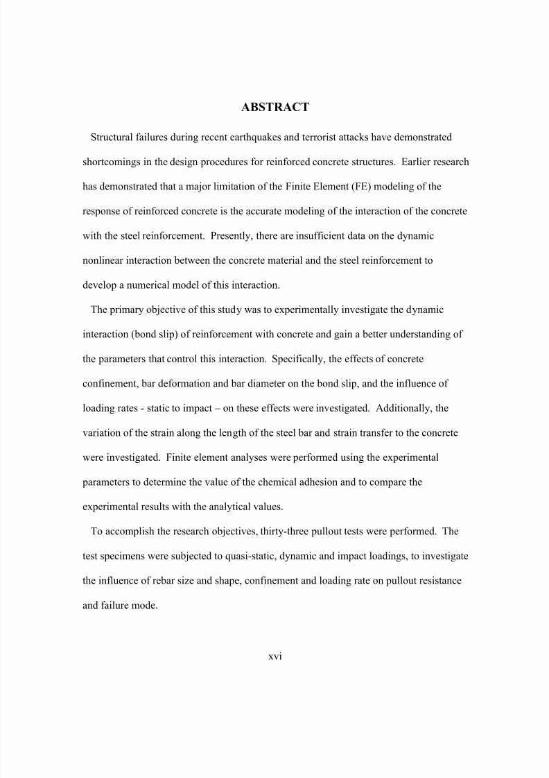
ABSTRACT
Structural failures during recent earthquakes and terrorist attacks have demonstrated
shortcomings in the design procedures for reinforced concrete structures. Earlier research
has demonstrated that a major limitation of the Finite Element (FE) modeling of the
response of reinforced concrete is the accurate modeling of the interaction of the concrete
with the steel reinforcement. Presently, there are insufficient data on the dynamic
nonlinear interaction between the concrete material and the steel reinforcement to
develop a numerical model of this interaction.
The primary objective of this study was to experimentally investigate the dynamic
interaction (bond slip) of reinforcement with concrete and gain a better understanding of
the parameters that control this interaction. Specifically, the effects of concrete
confinement, bar deformation and bar diameter on the bond slip, and the influence of
loading rates - static to impact – on these effects were investigated. Additionally, the
variation of the strain along the length of the steel bar and strain transfer to the concrete
were investigated. Finite element analyses were performed using the experimental
parameters to determine the value of the chemical adhesion and to compare the
experimental results with the analytical values.
To accomplish the research objectives, thirty-three pullout tests were performed. The
test specimens were subjected to quasi-static, dynamic and impact loadings, to investigate
the influence of rebar size and shape, confinement and loading rate on pullout resistance
and failure mode.

7/28/2019 Weathersby Dis
http://slidepdf.com/reader/full/weathersby-dis 17/280
7/28/2019 Weathersby Dis
http://slidepdf.com/reader/full/weathersby-dis 18/280
1
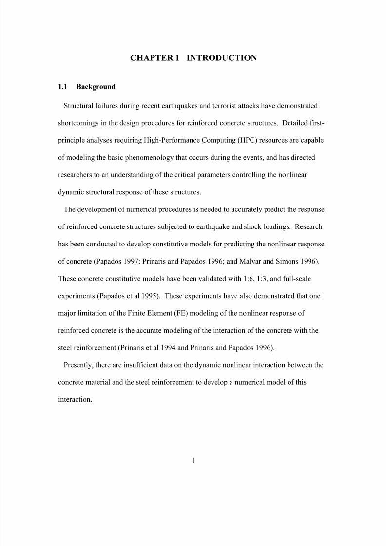
CHAPTER 1 INTRODUCTION
1.1 Background
Structural failures during recent earthquakes and terrorist attacks have demonstrated
shortcomings in the design procedures for reinforced concrete structures. Detailed first-
principle analyses requiring High-Performance Computing (HPC) resources are capable
of modeling the basic phenomenology that occurs during the events, and has directed
researchers to an understanding of the critical parameters controlling the nonlinear
dynamic structural response of these structures.
The development of numerical procedures is needed to accurately predict the response
of reinforced concrete structures subjected to earthquake and shock loadings. Research
has been conducted to develop constitutive models for predicting the nonlinear response
of concrete (Papados 1997; Prinaris and Papados 1996; and Malvar and Simons 1996).
These concrete constitutive models have been validated with 1:6, 1:3, and full-scale
experiments (Papados et al 1995). These experiments have also demonstrated that one
major limitation of the Finite Element (FE) modeling of the nonlinear response of
reinforced concrete is the accurate modeling of the interaction of the concrete with the
steel reinforcement (Prinaris et al 1994 and Prinaris and Papados 1996).
Presently, there are insufficient data on the dynamic nonlinear interaction between the
concrete material and the steel reinforcement to develop a numerical model of this
interaction.
7/28/2019 Weathersby Dis
http://slidepdf.com/reader/full/weathersby-dis 19/280
2
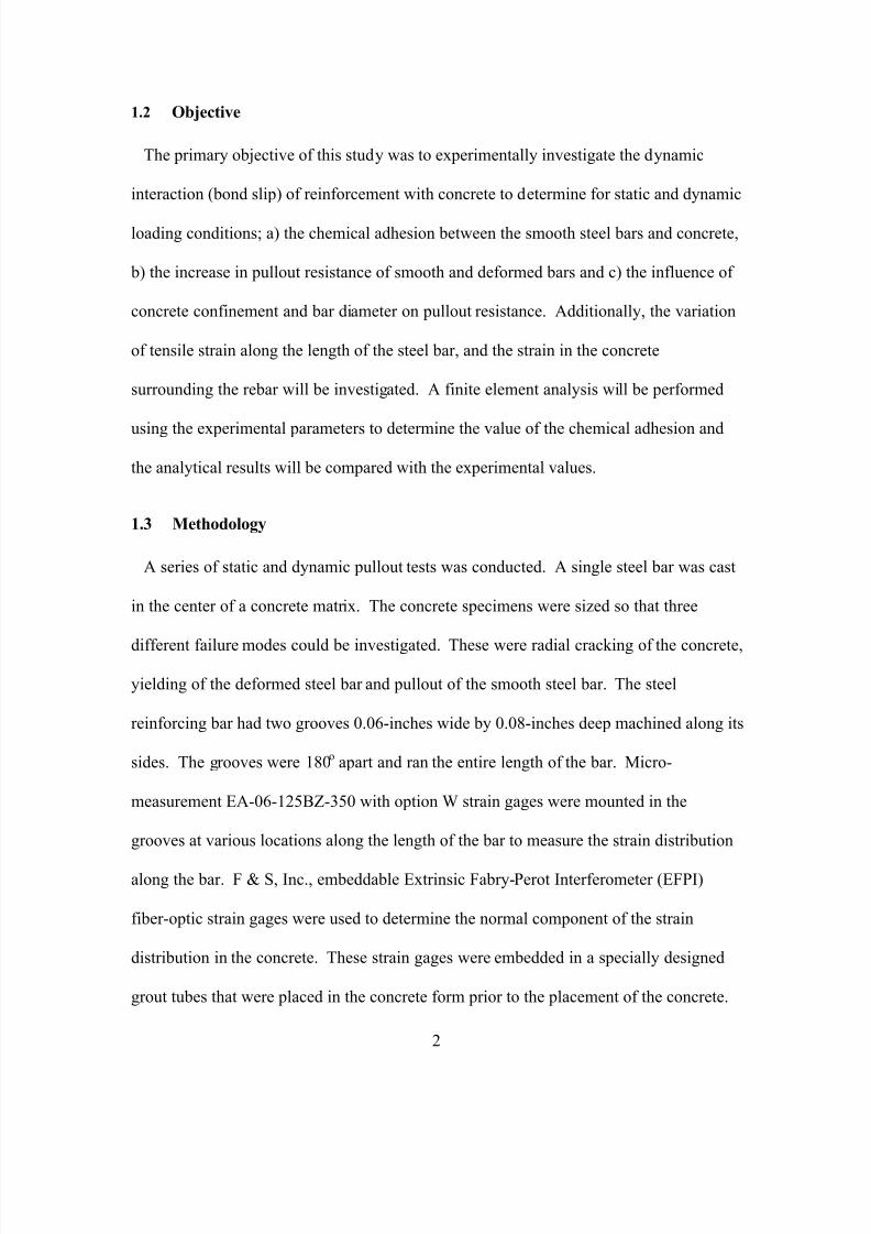
1.2 Objective
The primary objective of this study was to experimentally investigate the dynamic
interaction (bond slip) of reinforcement with concrete to determine for static and dynamic
loading conditions; a) the chemical adhesion between the smooth steel bars and concrete,
b) the increase in pullout resistance of smooth and deformed bars and c) the influence of
concrete confinement and bar diameter on pullout resistance. Additionally, the variation
of tensile strain along the length of the steel bar, and the strain in the concrete
surrounding the rebar will be investigated. A finite element analysis will be performed
using the experimental parameters to determine the value of the chemical adhesion and
the analytical results will be compared with the experimental values.
1.3 Methodology
A series of static and dynamic pullout tests was conducted. A single steel bar was cast
in the center of a concrete matrix. The concrete specimens were sized so that three
different failure modes could be investigated. These were radial cracking of the concrete,
yielding of the deformed steel bar and pullout of the smooth steel bar. The steel
reinforcing bar had two grooves 0.06-inches wide by 0.08-inches deep machined along its
sides. The grooves were 180o
apart and ran the entire length of the bar. Micro-
measurement EA-06-125BZ-350 with option W strain gages were mounted in the
grooves at various locations along the length of the bar to measure the strain distribution
along the bar. F & S, Inc., embeddable Extrinsic Fabry-Perot Interferometer (EFPI)
fiber-optic strain gages were used to determine the normal component of the strain
distribution in the concrete. These strain gages were embedded in a specially designed
grout tubes that were placed in the concrete form prior to the placement of the concrete.
7/28/2019 Weathersby Dis
http://slidepdf.com/reader/full/weathersby-dis 20/280
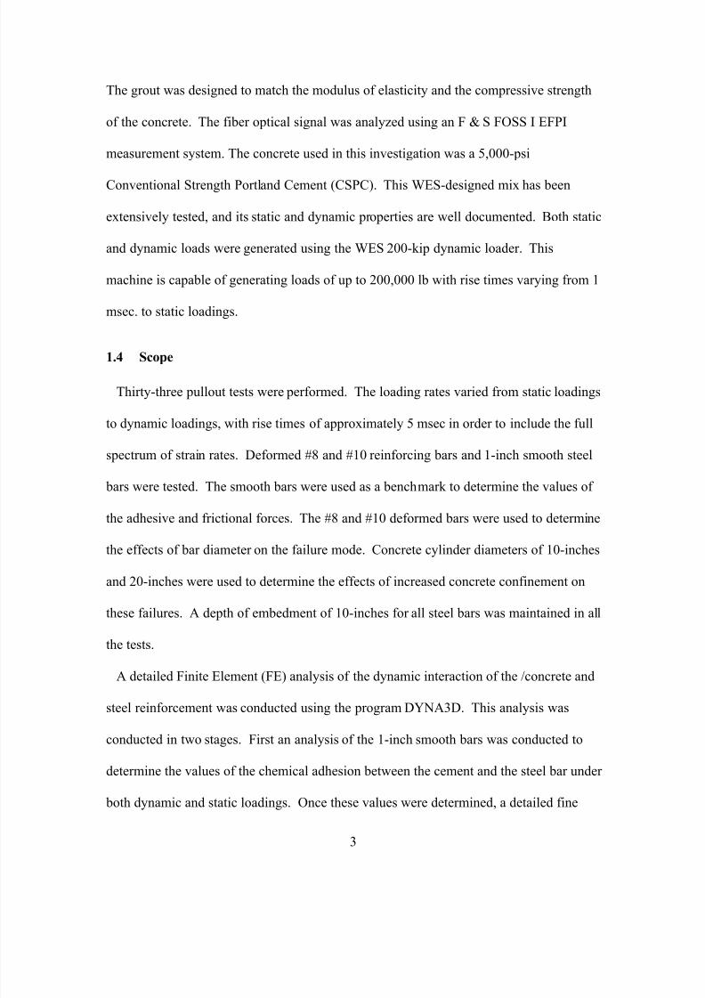
3
The grout was designed to match the modulus of elasticity and the compressive strength
of the concrete. The fiber optical signal was analyzed using an F & S FOSS I EFPI
measurement system. The concrete used in this investigation was a 5,000-psi
Conventional Strength Portland Cement (CSPC). This WES-designed mix has been
extensively tested, and its static and dynamic properties are well documented. Both static
and dynamic loads were generated using the WES 200-kip dynamic loader. This
machine is capable of generating loads of up to 200,000 lb with rise times varying from 1
msec. to static loadings.
1.4 Scope
Thirty-three pullout tests were performed. The loading rates varied from static loadings
to dynamic loadings, with rise times of approximately 5 msec in order to include the full
spectrum of strain rates. Deformed #8 and #10 reinforcing bars and 1-inch smooth steel
bars were tested. The smooth bars were used as a benchmark to determine the values of
the adhesive and frictional forces. The #8 and #10 deformed bars were used to determine
the effects of bar diameter on the failure mode. Concrete cylinder diameters of 10-inches
and 20-inches were used to determine the effects of increased concrete confinement on
these failures. A depth of embedment of 10-inches for all steel bars was maintained in all
the tests.
A detailed Finite Element (FE) analysis of the dynamic interaction of the /concrete and
steel reinforcement was conducted using the program DYNA3D. This analysis was
conducted in two stages. First an analysis of the 1-inch smooth bars was conducted to
determine the values of the chemical adhesion between the cement and the steel bar under
both dynamic and static loadings. Once these values were determined, a detailed fine

7/28/2019 Weathersby Dis
http://slidepdf.com/reader/full/weathersby-dis 21/280
4
grid analysis, which included modeling the individual deformations on the steel bar, was
conducted. Using the information gained on the first part of the FE analysis, the effects
of confinement and loading rates were investigated for the deformed bars.
7/28/2019 Weathersby Dis
http://slidepdf.com/reader/full/weathersby-dis 22/280
5
CHAPTER 2 LITERATURE REVIEW
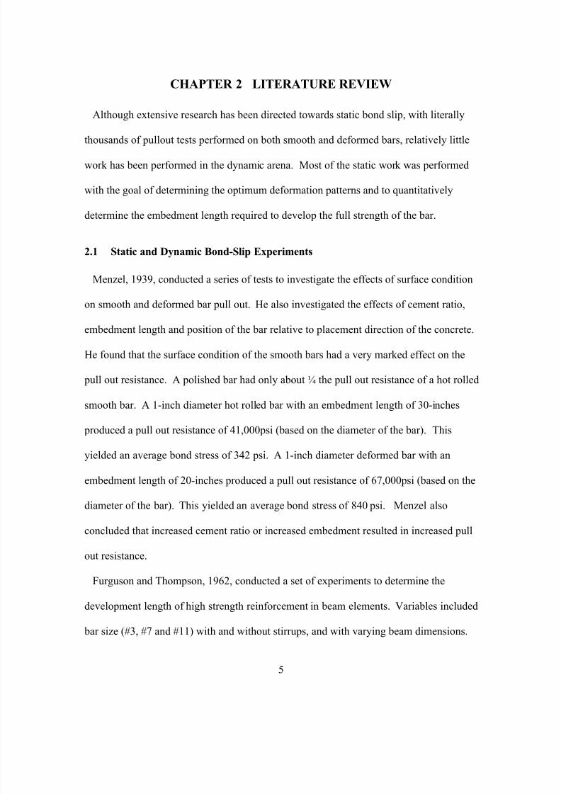
Although extensive research has been directed towards static bond slip, with literally
thousands of pullout tests performed on both smooth and deformed bars, relatively little
work has been performed in the dynamic arena. Most of the static work was performed
with the goal of determining the optimum deformation patterns and to quantitatively
determine the embedment length required to develop the full strength of the bar.
2.1 Static and Dynamic Bond-Slip Experiments
Menzel, 1939, conducted a series of tests to investigate the effects of surface condition
on smooth and deformed bar pull out. He also investigated the effects of cement ratio,
embedment length and position of the bar relative to placement direction of the concrete.
He found that the surface condition of the smooth bars had a very marked effect on the
pull out resistance. A polished bar had only about ¼ the pull out resistance of a hot rolled
smooth bar. A 1-inch diameter hot rolled bar with an embedment length of 30-inches
produced a pull out resistance of 41,000psi (based on the diameter of the bar). This
yielded an average bond stress of 342 psi. A 1-inch diameter deformed bar with an
embedment length of 20-inches produced a pull out resistance of 67,000psi (based on the
diameter of the bar). This yielded an average bond stress of 840 psi. Menzel also
concluded that increased cement ratio or increased embedment resulted in increased pull
out resistance.
Furguson and Thompson, 1962, conducted a set of experiments to determine the
development length of high strength reinforcement in beam elements. Variables included
bar size (#3, #7 and #11) with and without stirrups, and with varying beam dimensions.
7/28/2019 Weathersby Dis
http://slidepdf.com/reader/full/weathersby-dis 23/280
6
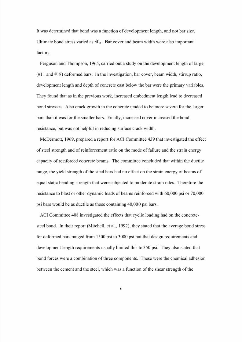
It was determined that bond was a function of development length, and not bar size.
Ultimate bond stress varied as √f’c. Bar cover and beam width were also important
factors.
Ferguson and Thompson, 1965, carried out a study on the development length of large
(#11 and #18) deformed bars. In the investigation, bar cover, beam width, stirrup ratio,
development length and depth of concrete cast below the bar were the primary variables.
They found that as in the previous work, increased embedment length lead to decreased
bond stresses. Also crack growth in the concrete tended to be more severe for the larger
bars than it was for the smaller bars. Finally, increased cover increased the bond
resistance, but was not helpful in reducing surface crack width.
McDermott, 1969, prepared a report for ACI Committee 439 that investigated the effect
of steel strength and of reinforcement ratio on the mode of failure and the strain energy
capacity of reinforced concrete beams. The committee concluded that within the ductile
range, the yield strength of the steel bars had no effect on the strain energy of beams of
equal static bending strength that were subjected to moderate strain rates. Therefore the
resistance to blast or other dynamic loads of beams reinforced with 60,000 psi or 70,000
psi bars would be as ductile as those containing 40,000 psi bars.
ACI Committee 408 investigated the effects that cyclic loading had on the concrete-
steel bond. In their report (Mitchell, et al., 1992), they stated that the average bond stress
for deformed bars ranged from 1500 psi to 3000 psi but that design requirements and
development length requirements usually limited this to 350 psi. They also stated that
bond forces were a combination of three components. These were the chemical adhesion
between the cement and the steel, which was a function of the shear strength of the
7/28/2019 Weathersby Dis
http://slidepdf.com/reader/full/weathersby-dis 24/280
7
concrete, the mechanical interlocking of the steel deformations and the concrete, and the
friction between the concrete and the steel.
An in-depth study of bond slip under impact loading for plain, polypropylene fiber
reinforced and steel reinforced concrete was performed (Yan 1992). Dynamic loads were
generated using a 345-kg mass drop weight impact machine. The experiments consisted
of both pullout and push-in tests. For both types of tests, the experimental work was
carried out for three different types of loading: static, dynamic, and impact loading,
which covered a stress rate ranging from 0.5 x 10⁻⁸
to 0.5 x 10⁻²
Mpa/s. The other
important variables considered in the experimental study were: two different types of
reinforcing bars (smooth and deformed), two different concrete compressive strengths
(normal and high), two different fibers (polypropylene and steel), different fiber contents
(0.1 %, 0.5 %, and 1.0 % by volume), and surface conditions (epoxy coated and
uncoated). The load applied to the rebar and the strains along the rebar were measured
directly. The axial force in the concrete was determined from the difference between two
consecutive strain readings in the steel bar, and the normal force in the concrete was
calculated based on a static equilibrium analysis.
It was found that for smooth rebar, there existed a linear bond-slip relationship under
both static and high-rate loading. Different loading rates, compressive strengths, types of
fibers, and fiber contents were found to have no significant effect on the bond-slip
relationship.
For deformed bars, the shear mechanism due to the ribs bearing on the concrete was
found to play a major role in the bond resistance. The bond stress-slip relationship under
a dynamic loading changes with time and is different at different points along the
7/28/2019 Weathersby Dis
http://slidepdf.com/reader/full/weathersby-dis 25/280
8
reinforcing bar. In terms of the average bond stress-slip relationship over the time period
and the embedment length, different loading rates, compressive strengths, types of fibers,
and fiber contents were found to have a great influence on this relationship. Higher
loading rates, higher compressive strengths, and steel fibers at a sufficient content
significantly increased the bond-resistance capacity and the fracture energy in bond
failure. All of these factors had a great influence on the stress distributions in the
concrete, the slips at the interface between the rebar and the concrete, and the crack
development. It was also found that there is always higher bond resistance for push-in
loading than for pullout loading.
In the analytical study, FE analysis with fracture mechanics was carried out to
investigate the bond phenomenon under high rate loading. The analytical model took
into account the chemical adhesion, the frictional resistance, and the rib-bearing
mechanism. In the analysis, solid isoperimetric elements with 20 nodes and 60 degrees
of freedom were employed for the rebar and concrete before cracking. After cracking,
the concrete elements were replaced by quadratic singularity elements, which were
quarter-point elements able to model curved crack fronts. A special interface element,
the “bond-link element,” was adopted to model the connection between the reinforcing
bar and concrete. It connected two nodes and had no physical thickness, therefore it
could be thought of conceptually as consisting of two orthogonal springs, which
simulated the mechanical properties in the connection, i.e. they transmitted the shear and
normal forces between two nodes
A set of dynamic experiments with the goal of quantitatively defining the bond-stress
relationship for inclusion in FE analyses was performed (Vos 1983). Vos used a Split
7/28/2019 Weathersby Dis
http://slidepdf.com/reader/full/weathersby-dis 26/280
9
Hopkinson Bar test device to load his samples. In this work, only one bar diameter (10
mm) and one embedment length (3d = 30 mm) were used. Three different concrete
strengths (22, 45, and 55 N/mm2) were tested. Additionally, three types of steel
reinforcement (plain, deformed, and strands) were used. Vos reached conclusions similar
to those reached by Yan; namely, that the bond resistance of plain bars is independent of
loading rate and concrete strength. The deformed bar on the other hand showed a marked
increase in bond resistance with an increase in either loading rate or concrete strength.
2.2 Strain Rate Effects on Concrete
Bentur et al 1986 and Banthia et al 1988 conducted a series of experiments to
investigate the behavior of concrete under impact loading. Their work involved the
testing and analysis of both plain and conventionally reinforced beams subjected to
impact loads. The test specimens had a length by width by depth of 1,400 by 100 by 125
mm and a span length of 960 mm. The dynamic loads were generated by a drop weight
machine, which had the capability of dropping a 345-kg mass from a height of 3 m.
From these tests, it was determined that concrete can withstand a higher peak bending
load under impact than under static conditions. They concluded that concrete is a
significantly stress-rate dependent material that is stronger and more energy absorbing
under impact than static loading. Moreover, in the beams made with deformed bars, the
reinforcing bars frequently failed in a ductile mode of failure at the point of impact. This,
they concluded, was due to the fact that under impact loading, with the maximum load
being reached in less than 1 msec, there was not enough time for extensive bond slip to
occur along the length of the bar. Instead, the steel deformation was confined primarily
to the region, only a few centimeters long, beneath the point of impact, exceeding the
7/28/2019 Weathersby Dis
http://slidepdf.com/reader/full/weathersby-dis 27/280
10
strain capability of the steel in this region. This was clearly related to strain rate; under
quasi-static loading, beams deflected to the same degree showed no evidence of steel
failure; instead, there were signs of cracking and de-bonding along a significant length of
the reinforcing bar.
2.3 Cracking of Concrete Around Deformed Bars
A set of experiments was performed to study the formation of cracks in concrete
surrounding a deformed reinforcing bar (Goto 1971). In these tests, a single deformed
reinforcing bar was encased in a long concrete prism, and an axial tension load was
applied to the exposed end of the bar. Ink was injected into the concrete to mark the
cracks, and the specimens were split longitudinally along the bar. The crack patterns
were then analyzed and recorded. Goto reported three different types of cracks: lateral,
internal and longitudinal. Lateral cracks are visible at the concrete surface and are at
right angles to the bar axis. Internal cracks form around the deformed bars shortly after
the formation of the lateral cracks. These small cracks do not appear at the concrete
surface. Longitudinal cracks are formed at high steel-stress levels. In this case, the
concrete adjacent to existing lateral cracks also cracks in the direction of the bar axis.
A series of pullout tests were performed to determine the effect the depth of cover had
on the bond stress and to determine the bond stress at different levels of concrete
cracking (Tepfers 1979). In these tests, a single reinforcing bar was cast eccentrically in
a concrete prism. The specimens were 200 mm by 150 mm with a depth of 3.13 bar
diameters. The bars were placed at distances varying from 16 mm to over 90 mm from
the edge of the sample. Equations were developed expressing the bond stress at three
different stages based on the crack condition of the concrete cover. These were the un-
7/28/2019 Weathersby Dis
http://slidepdf.com/reader/full/weathersby-dis 28/280
11
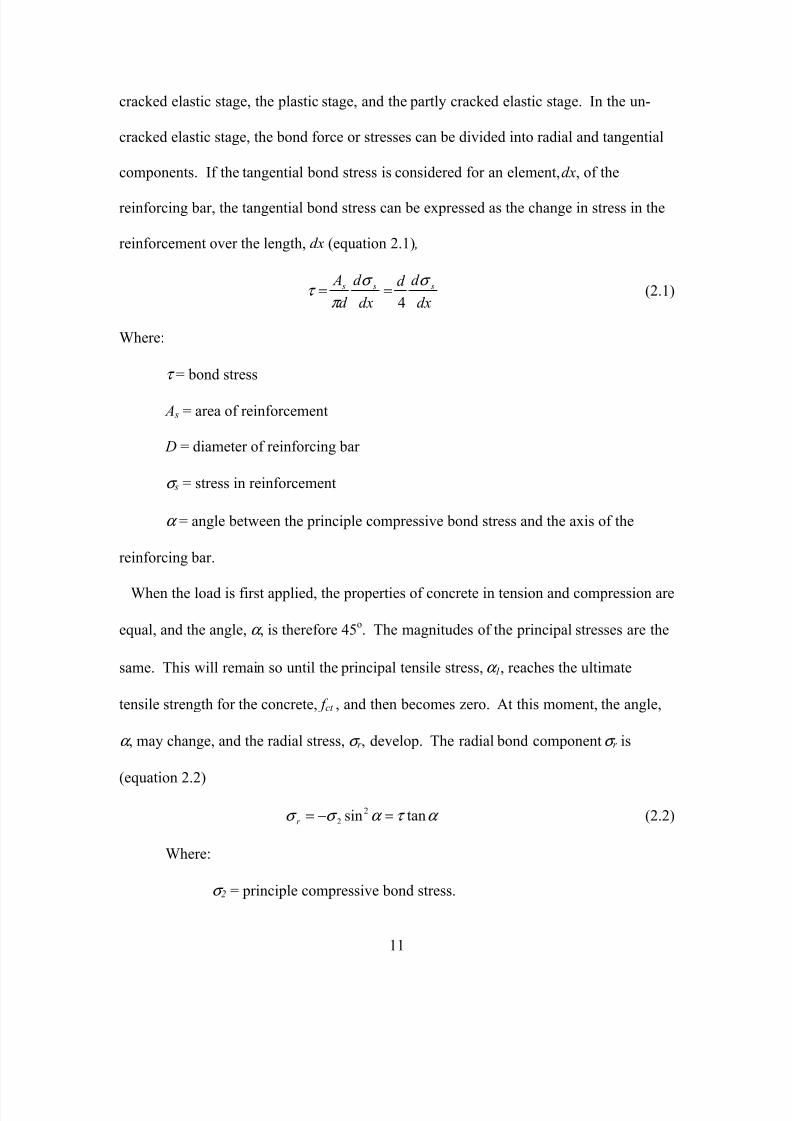
cracked elastic stage, the plastic stage, and the partly cracked elastic stage. In the un-
cracked elastic stage, the bond force or stresses can be divided into radial and tangential
components. If the tangential bond stress is considered for an element, dx, of the
reinforcing bar, the tangential bond stress can be expressed as the change in stress in the
reinforcement over the length, dx (equation 2.1) ,
dx
d d
dx
d
d
A s s s σ σ
π τ
4== (2.1)
Where:
τ = bond stress
A s = area of reinforcement
D = diameter of reinforcing bar
σ s = stress in reinforcement
α = angle between the principle compressive bond stress and the axis of the
reinforcing bar.
When the load is first applied, the properties of concrete in tension and compression are
equal, and the angle, α , is therefore 45o. The magnitudes of the principal stresses are the
same. This will remain so until the principal tensile stress, α 1, reaches the ultimate
tensile strength for the concrete, f ct , and then becomes zero. At this moment, the angle,
α , may change, and the radial stress, σ r , develop. The radial bond component σ r is
(equation 2.2)
α τ α σ σ tansin2
2 =−=r (2.2)
Where:
σ 2 = principle compressive bond stress.
7/28/2019 Weathersby Dis
http://slidepdf.com/reader/full/weathersby-dis 29/280
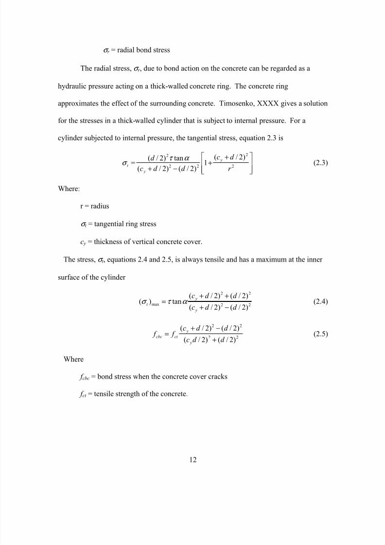
12
σ r = radial bond stress
The radial stress, σ r , due to bond action on the concrete can be regarded as a
hydraulic pressure acting on a thick-walled concrete ring. The concrete ring
approximates the effect of the surrounding concrete. Timosenko, XXXX gives a solution
for the stresses in a thick-walled cylinder that is subject to internal pressure. For a
cylinder subjected to internal pressure, the tangential stress, equation 2.3 is
++
−+=
2
2
22
2 )2/(1
)2/()2/(
tan)2/(
r
d c
d d c
d y
y
t
α τ σ (2.3)
Where:
r = radius
σ t = tangential ring stress
c y = thickness of vertical concrete cover.
The stress, σ t , equations 2.4 and 2.5, is always tensile and has a maximum at the inner
surface of the cylinder
22
22
max)2/()2/(
)2/()2/(tan)(
d d c
d d c
y
y
t −+
++= α τ σ (2.4)
22
22
)2/()2/(
)2/()2/(
d d c
d d c f f
y
y
ct cbc+
−+= (2.5)
Where
f cbc = bond stress when the concrete cover cracks
f ct = tensile strength of the concrete.
7/28/2019 Weathersby Dis
http://slidepdf.com/reader/full/weathersby-dis 30/280
13
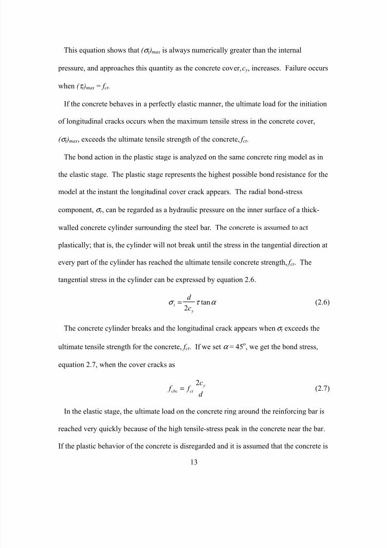
This equation shows that ( σ t )max is always numerically greater than the internal
pressure, and approaches this quantity as the concrete cover, c y, increases. Failure occurs
when ( τ t )max = f ct .
If the concrete behaves in a perfectly elastic manner, the ultimate load for the initiation
of longitudinal cracks occurs when the maximum tensile stress in the concrete cover,
( σ t )max, exceeds the ultimate tensile strength of the concrete, f ct .
The bond action in the plastic stage is analyzed on the same concrete ring model as in
the elastic stage. The plastic stage represents the highest possible bond resistance for the
model at the instant the longitudinal cover crack appears. The radial bond-stress
component, σ r , can be regarded as a hydraulic pressure on the inner surface of a thick-
walled concrete cylinder surrounding the steel bar. The concrete is assumed to act
plastically; that is, the cylinder will not break until the stress in the tangential direction at
every part of the cylinder has reached the ultimate tensile concrete strength, f ct . The
tangential stress in the cylinder can be expressed by equation 2.6.
α τ σ tan2 y
t c
d = (2.6)
The concrete cylinder breaks and the longitudinal crack appears when σ t exceeds the
ultimate tensile strength for the concrete, f ct . If we set α = 45o, we get the bond stress,
equation 2.7, when the cover cracks as
d c f f y
ct cbc2= (2.7)
In the elastic stage, the ultimate load on the concrete ring around the reinforcing bar is
reached very quickly because of the high tensile-stress peak in the concrete near the bar.
If the plastic behavior of the concrete is disregarded and it is assumed that the concrete is
7/28/2019 Weathersby Dis
http://slidepdf.com/reader/full/weathersby-dis 31/280
14
a completely elastic material, an internal crack will start when the peak tensile stress
exceeds the ultimate tensile stress of the concrete. The longitudinal crack starting at this
point will not penetrate through the concrete cover if the load-carrying capacity of the
concrete ring has not yet been reached at that moment.
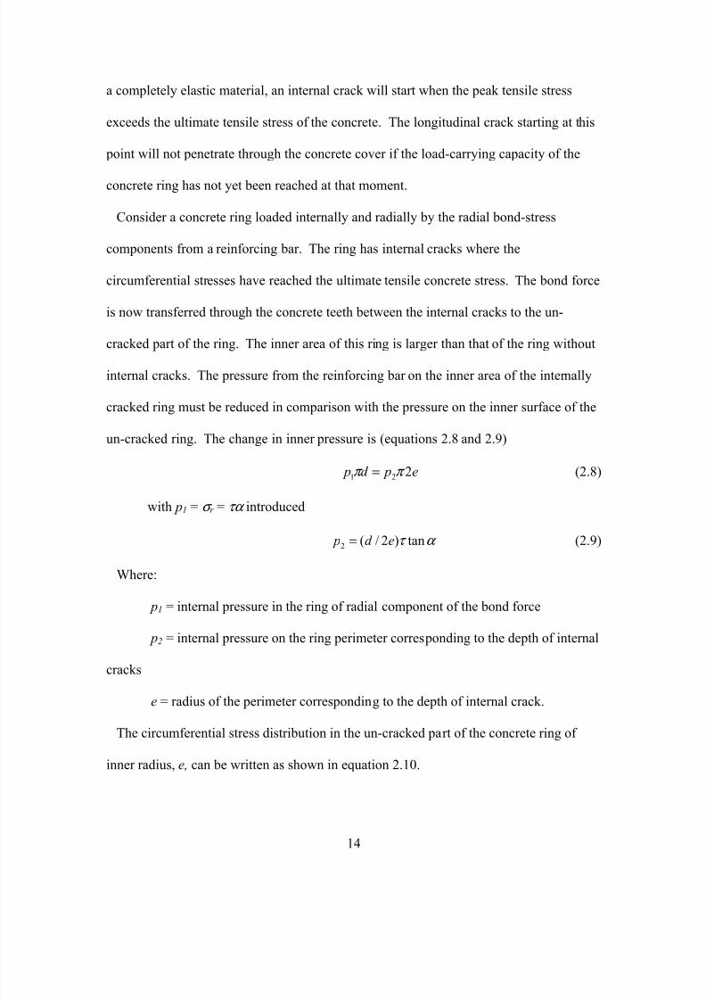
Consider a concrete ring loaded internally and radially by the radial bond-stress
components from a reinforcing bar. The ring has internal cracks where the
circumferential stresses have reached the ultimate tensile concrete stress. The bond force
is now transferred through the concrete teeth between the internal cracks to the un-
cracked part of the ring. The inner area of this ring is larger than that of the ring without
internal cracks. The pressure from the reinforcing bar on the inner area of the internally
cracked ring must be reduced in comparison with the pressure on the inner surface of the
un-cracked ring. The change in inner pressure is (equations 2.8 and 2.9)
e pd p 221π π = (2.8)
with p1 = σ r = τα introduced
α τ tan)2/(2 ed p = (2.9)
Where:
p1 = internal pressure in the ring of radial component of the bond force
p2 = internal pressure on the ring perimeter corresponding to the depth of internal
cracks
e = radius of the perimeter corresponding to the depth of internal crack.
The circumferential stress distribution in the un-cracked part of the concrete ring of
inner radius, e, can be written as shown in equation 2.10.
7/28/2019 Weathersby Dis
http://slidepdf.com/reader/full/weathersby-dis 32/280
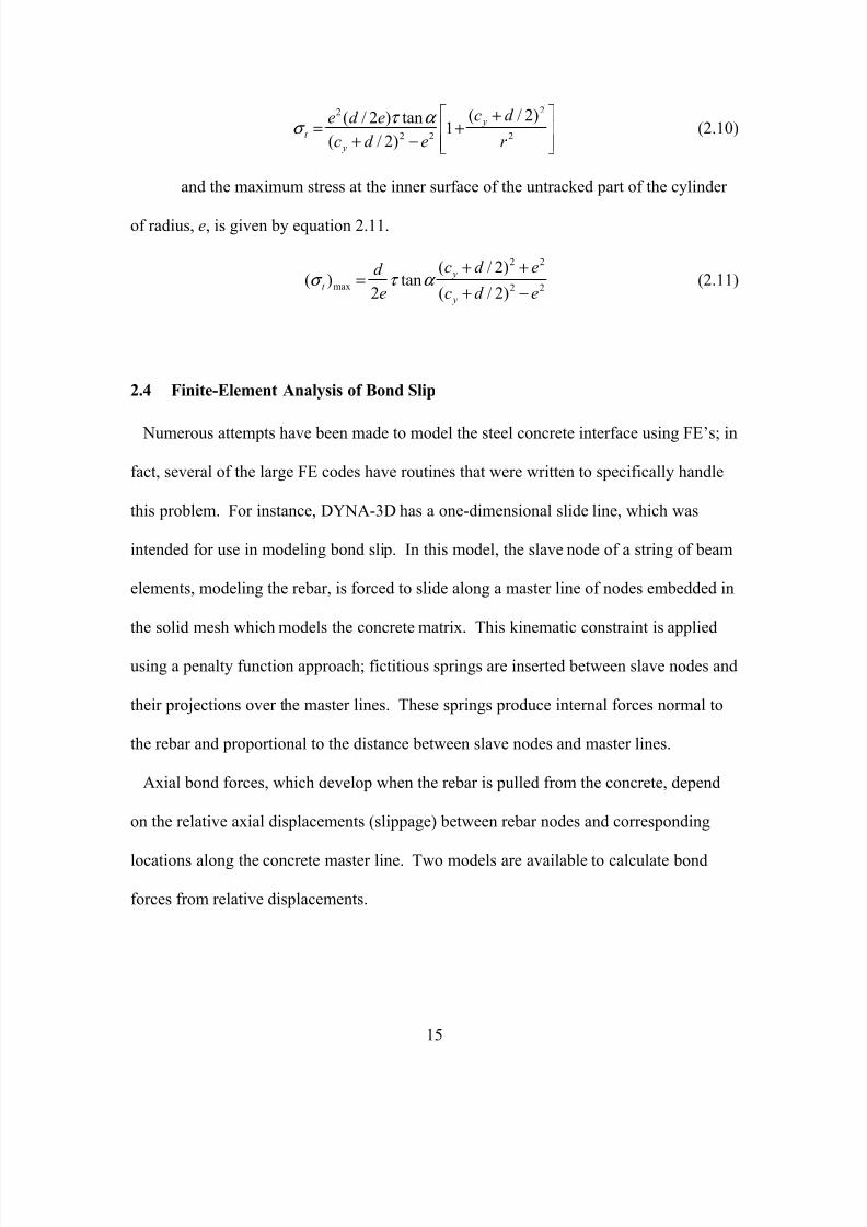
15
++
−+=
2
2
22
2 )2/(1
)2/(
tan)2/(
r
d c
ed c
ed e y
y
t
α τ σ (2.10)
and the maximum stress at the inner surface of the untracked part of the cylinder
of radius, e, is given by equation 2.11.
22
22
max)2/(
)2/(tan
2)(
ed c
ed c
e
d
y
y
t −+
++= α τ σ (2.11)
2.4 Finite-Element Analysis of Bond Slip
Numerous attempts have been made to model the steel concrete interface using FE’s; in
fact, several of the large FE codes have routines that were written to specifically handle
this problem. For instance, DYNA-3D has a one-dimensional slide line, which was
intended for use in modeling bond slip. In this model, the slave node of a string of beam
elements, modeling the rebar, is forced to slide along a master line of nodes embedded in
the solid mesh which models the concrete matrix. This kinematic constraint is applied
using a penalty function approach; fictitious springs are inserted between slave nodes and
their projections over the master lines. These springs produce internal forces normal to
the rebar and proportional to the distance between slave nodes and master lines.
Axial bond forces, which develop when the rebar is pulled from the concrete, depend
on the relative axial displacements (slippage) between rebar nodes and corresponding
locations along the concrete master line. Two models are available to calculate bond
forces from relative displacements.
7/28/2019 Weathersby Dis
http://slidepdf.com/reader/full/weathersby-dis 33/280
16
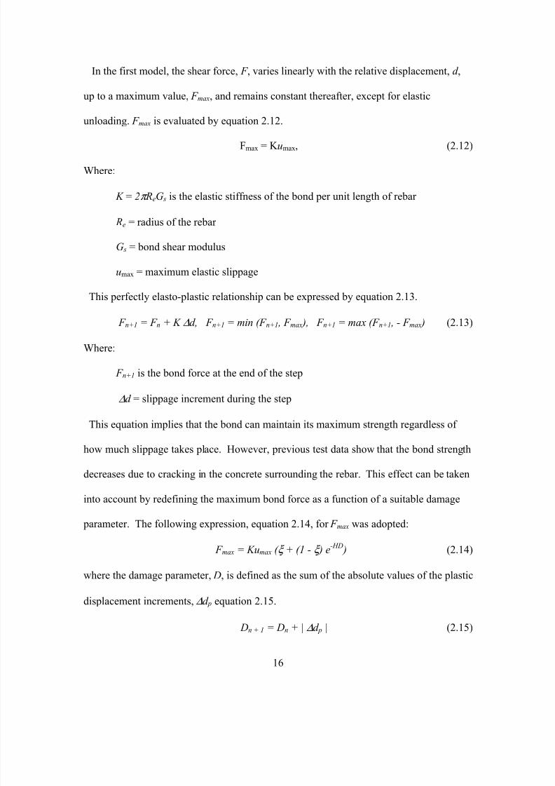
In the first model, the shear force, F , varies linearly with the relative displacement, d ,
up to a maximum value, F max, and remains constant thereafter, except for elastic
unloading. F max is evaluated by equation 2.12.
Fmax = K umax, (2.12)
Where:
K = 2π ReG s is the elastic stiffness of the bond per unit length of rebar
Re = radius of the rebar
G s = bond shear modulus
umax = maximum elastic slippage
This perfectly elasto-plastic relationship can be expressed by equation 2.13.
F n+1 = F n + K ∆d, F n+1 = min (F n+1 , F max ), F n+1 = max (F n+1 , - F max ) (2.13)
Where:
F n+1 is the bond force at the end of the step
∆d = slippage increment during the step
This equation implies that the bond can maintain its maximum strength regardless of
how much slippage takes place. However, previous test data show that the bond strength
decreases due to cracking in the concrete surrounding the rebar. This effect can be taken
into account by redefining the maximum bond force as a function of a suitable damage
parameter. The following expression, equation 2.14, for F max was adopted:
F max = Kumax ( ξ + (1 - ξ ) e-HD
) (2.14)
where the damage parameter, D, is defined as the sum of the absolute values of the plastic
displacement increments, ∆d p equation 2.15.
Dn + 1 = Dn + | ∆d p | (2.15)
7/28/2019 Weathersby Dis
http://slidepdf.com/reader/full/weathersby-dis 34/280
17
and H is a decay parameter obtained from test datum, and ξ is the fraction of residual
strength after the bond is completely degraded.
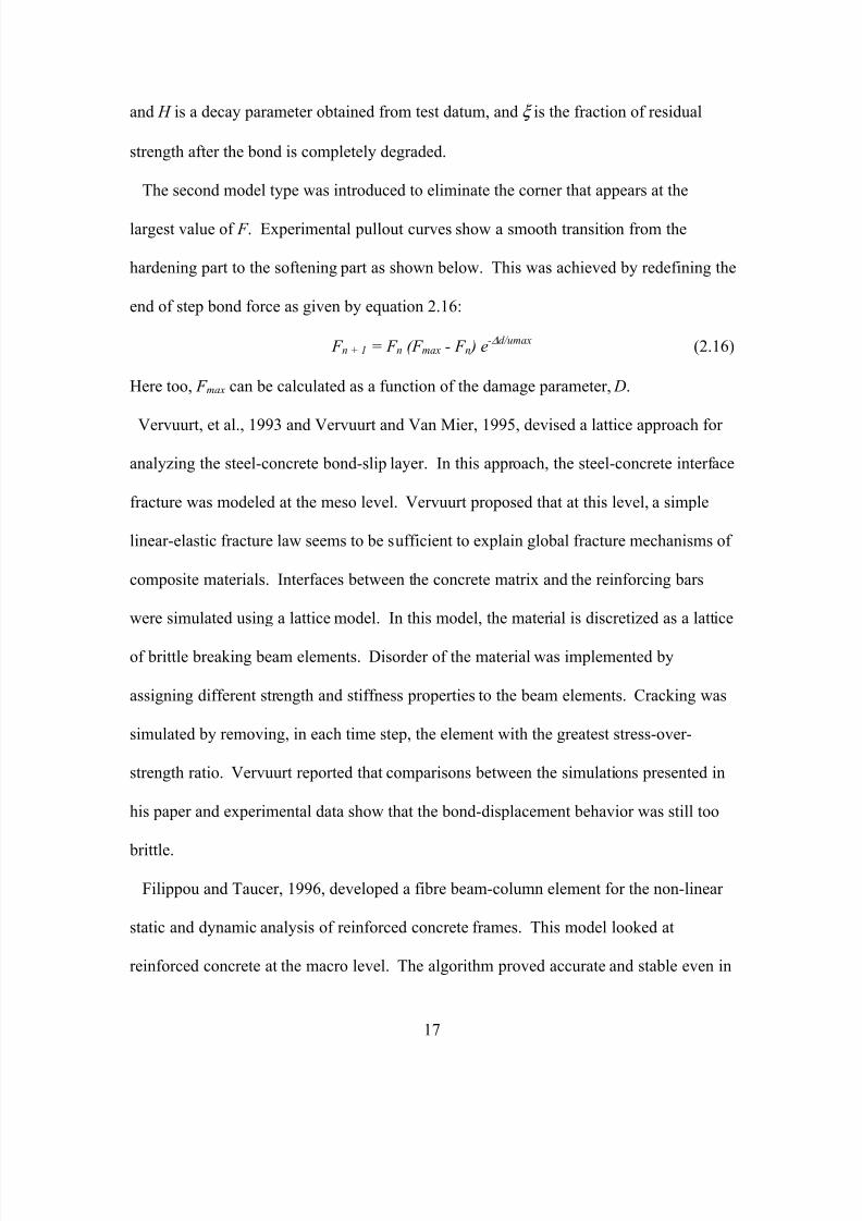
The second model type was introduced to eliminate the corner that appears at the
largest value of F . Experimental pullout curves show a smooth transition from the
hardening part to the softening part as shown below. This was achieved by redefining the
end of step bond force as given by equation 2.16:
F n + 1 = F n (F max - F n ) e-∆d/umax
(2.16)
Here too, F max can be calculated as a function of the damage parameter, D.
Vervuurt, et al., 1993 and Vervuurt and Van Mier, 1995, devised a lattice approach for
analyzing the steel-concrete bond-slip layer. In this approach, the steel-concrete interface
fracture was modeled at the meso level. Vervuurt proposed that at this level, a simple
linear-elastic fracture law seems to be sufficient to explain global fracture mechanisms of
composite materials. Interfaces between the concrete matrix and the reinforcing bars
were simulated using a lattice model. In this model, the material is discretized as a lattice
of brittle breaking beam elements. Disorder of the material was implemented by
assigning different strength and stiffness properties to the beam elements. Cracking was
simulated by removing, in each time step, the element with the greatest stress-over-
strength ratio. Vervuurt reported that comparisons between the simulations presented in
his paper and experimental data show that the bond-displacement behavior was still too
brittle.
Filippou and Taucer, 1996, developed a fibre beam-column element for the non-linear
static and dynamic analysis of reinforced concrete frames. This model looked at
reinforced concrete at the macro level. The algorithm proved accurate and stable even in

7/28/2019 Weathersby Dis
http://slidepdf.com/reader/full/weathersby-dis 35/280
18
the presence of strength loss, thereby making it capable of modeling the highly non-linear
behavior of reinforced concrete members under dynamic loading.
7/28/2019 Weathersby Dis
http://slidepdf.com/reader/full/weathersby-dis 36/280
19
CHAPTER 3 EXPERIMENTAL PROCEDURES
A series of thirty-three dynamic and quasi-static experiments were conducted to
experimentally evaluate the effects that confinement, bar diameter, bar deformation and
loading rate had on the interaction of steel reinforcement and a concrete matrix.
3.1 Material Properties
The static and dynamic properties of the concrete and steel bars used in this
investigation were determined in order to provide material properties for the finite
element analysis.
3.1.1 Concrete Properties
The concrete selected for the experiment was a WES developed mix referred to as
Conventional Strength Portland Cement (CSPC). This mix was selected because its static
and dynamic properties are well documented and it is representative of the types of
concrete used in conventional construction. CSPC has a design compressive strength of
5,600 psi, direct tensile strength of 520 psi and a modulus of elasticity in compression
(Ec) of 6.1 x 10⁶
psi. The mix design is shown in Table 3.1. The static and dynamic
properties of CSPC and its development are documented (Nealy, 1991).
Quality control specimens taken from the batches used in casting the test specimens
indicated that the actual compressive strength of the concrete was greater than the design
strength. The static compressive strength was 7,650 psi with a modulus of elasticity of
6.45 x 10⁶
psi. The compressive strength decreased to 7,250 psi but the modulus of
elasticity increased to 6.95 x 10⁶
psi as the loading rate was increased to 200 msec.
When the loading rate was further increased to 5 msec, the compressive strength returned
7/28/2019 Weathersby Dis
http://slidepdf.com/reader/full/weathersby-dis 37/280
20
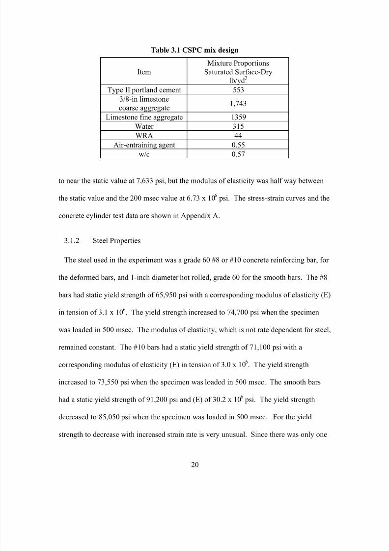
Table 3.1 CSPC mix design
Item
Mixture Proportions
Saturated Surface-Drylb/yd
3
Type II portland cement 553
3/8-in limestonecoarse aggregate
1,743
Limestone fine aggregate 1359
Water 315
WRA 44
Air-entraining agent 0.55
w/c 0.57
to near the static value at 7,633 psi, but the modulus of elasticity was half way between
the static value and the 200 msec value at 6.73 x 10⁶
psi. The stress-strain curves and the
concrete cylinder test data are shown in Appendix A.
3.1.2 Steel Properties
The steel used in the experiment was a grade 60 #8 or #10 concrete reinforcing bar, for
the deformed bars, and 1-inch diameter hot rolled, grade 60 for the smooth bars. The #8
bars had static yield strength of 65,950 psi with a corresponding modulus of elasticity (E)
in tension of 3.1 x 10⁶. The yield strength increased to 74,700 psi when the specimen
was loaded in 500 msec. The modulus of elasticity, which is not rate dependent for steel,
remained constant. The #10 bars had a static yield strength of 71,100 psi with a
corresponding modulus of elasticity (E) in tension of 3.0 x 10⁶. The yield strength
increased to 73,550 psi when the specimen was loaded in 500 msec. The smooth bars
had a static yield strength of 91,200 psi and (E) of 30.2 x 10⁶
psi. The yield strength
decreased to 85,050 psi when the specimen was loaded in 500 msec. For the yield
strength to decrease with increased strain rate is very unusual. Since there was only one
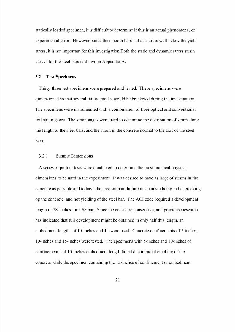
7/28/2019 Weathersby Dis
http://slidepdf.com/reader/full/weathersby-dis 38/280
21
statically loaded specimen, it is difficult to determine if this is an actual phenomena, or
experimental error. However, since the smooth bars fail at a stress well below the yield
stress, it is not important for this investigation Both the static and dynamic stress strain
curves for the steel bars is shown in Appendix A.
3.2 Test Specimens
Thirty-three test specimens were prepared and tested. These specimens were
dimensioned so that several failure modes would be bracketed during the investigation.
The specimens were instrumented with a combination of fiber optical and conventional
foil strain gages. The strain gages were used to determine the distribution of strain along
the length of the steel bars, and the strain in the concrete normal to the axis of the steel
bars.
3.2.1 Sample Dimensions
A series of pullout tests were conducted to determine the most practical physical
dimensions to be used in the experiment. It was desired to have as large of strains in the
concrete as possible and to have the predominant failure mechanism being radial cracking
og the concrete, and not yielding of the steel bar. The ACI code required a development
length of 28-inches for a #8 bar. Since the codes are conseritive, and previouse research
has indicated that full development might be obtained in only half this length, an
embedment lengths of 10-inches and 14-were used. Concrete confinements of 5-inches,
10-inches and 15-inches were tested. The specimens with 5-inches and 10-inches of
confinement and 10-inches embedment length failed due to radial cracking of the
concrete while the specimen containing the 15-inches of confinement or embedment
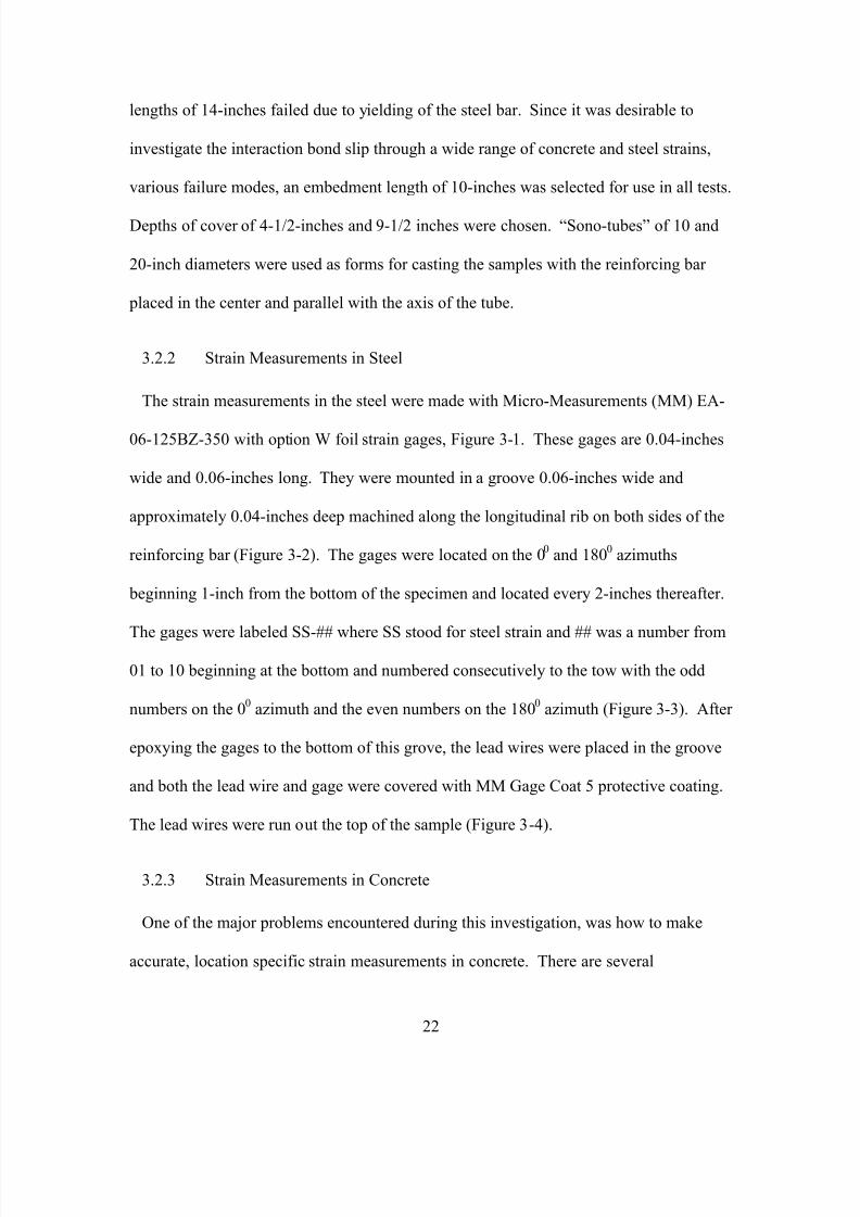
7/28/2019 Weathersby Dis
http://slidepdf.com/reader/full/weathersby-dis 39/280
22
lengths of 14-inches failed due to yielding of the steel bar. Since it was desirable to
investigate the interaction bond slip through a wide range of concrete and steel strains,
various failure modes, an embedment length of 10-inches was selected for use in all tests.
Depths of cover of 4-1/2-inches and 9-1/2 inches were chosen. “Sono-tubes” of 10 and
20-inch diameters were used as forms for casting the samples with the reinforcing bar
placed in the center and parallel with the axis of the tube.
3.2.2 Strain Measurements in Steel
The strain measurements in the steel were made with Micro-Measurements (MM) EA-
06-125BZ-350 with option W foil strain gages, Figure 3-1. These gages are 0.04-inches
wide and 0.06-inches long. They were mounted in a groove 0.06-inches wide and
approximately 0.04-inches deep machined along the longitudinal rib on both sides of the
reinforcing bar (Figure 3-2). The gages were located on the 00
and 1800
azimuths
beginning 1-inch from the bottom of the specimen and located every 2-inches thereafter.
The gages were labeled SS-## where SS stood for steel strain and ## was a number from
01 to 10 beginning at the bottom and numbered consecutively to the tow with the odd
numbers on the 00
azimuth and the even numbers on the 1800
azimuth (Figure 3-3). After
epoxying the gages to the bottom of this grove, the lead wires were placed in the groove
and both the lead wire and gage were covered with MM Gage Coat 5 protective coating.
The lead wires were run out the top of the sample (Figure 3-4).
3.2.3 Strain Measurements in Concrete
One of the major problems encountered during this investigation, was how to make
accurate, location specific strain measurements in concrete. There are several
7/28/2019 Weathersby Dis
http://slidepdf.com/reader/full/weathersby-dis 40/280
23
commercially available concrete strain gages on the market; however, none were suitable
for this investigation. These gages ranged in size from 4 to 9 inches in length and were
designed to measure the average strain over that length. Since the concrete strain that
Figure 3-1 Micro-Measurements foil strain gauge
Figure 3-2 Steel bar prior to placement of strain gauges
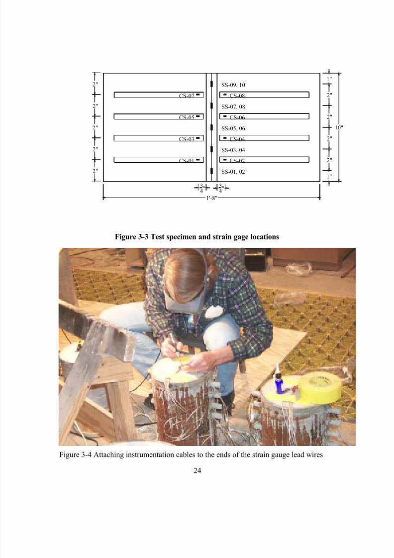
7/28/2019 Weathersby Dis
http://slidepdf.com/reader/full/weathersby-dis 41/280
24
1"
2"
2"
2"
2"
1"
10"
SS-03, 04
SS-01, 02
SS-05, 06
SS-07, 08
SS-09, 10
34"
34"
1'-8"
CS-02CS-01
CS-03
CS-05
CS-07
CS-04
CS-06
CS-08
2"
2"
2"
2"
2"
Figure 3-3 Test specimen and strain gage locations
Figure 3-4 Attaching instrumentation cables to the ends of the strain gauge lead wires
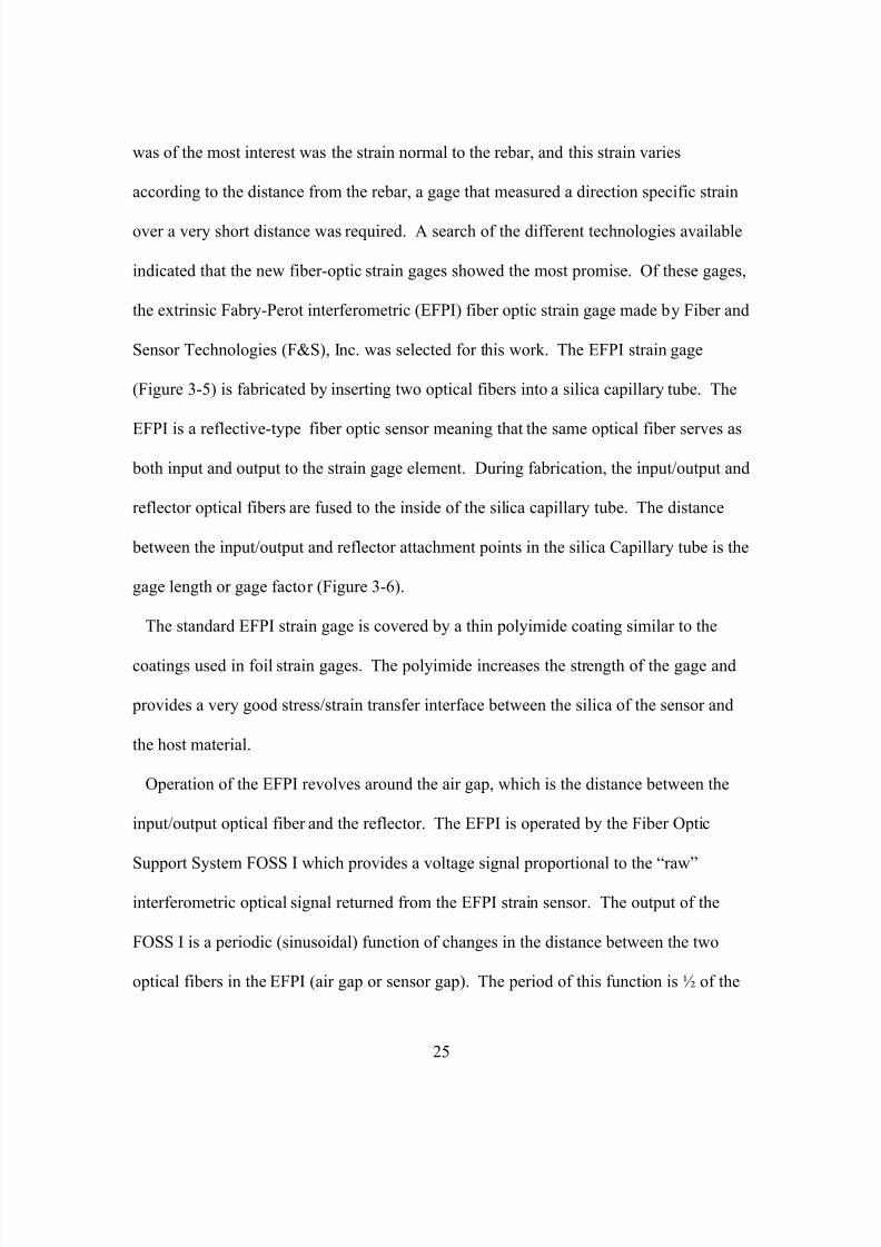
7/28/2019 Weathersby Dis
http://slidepdf.com/reader/full/weathersby-dis 42/280
25
was of the most interest was the strain normal to the rebar, and this strain varies
according to the distance from the rebar, a gage that measured a direction specific strain
over a very short distance was required. A search of the different technologies available
indicated that the new fiber-optic strain gages showed the most promise. Of these gages,
the extrinsic Fabry-Perot interferometric (EFPI) fiber optic strain gage made by Fiber and
Sensor Technologies (F&S), Inc. was selected for this work. The EFPI strain gage
(Figure 3-5) is fabricated by inserting two optical fibers into a silica capillary tube. The
EFPI is a reflective-type fiber optic sensor meaning that the same optical fiber serves as
both input and output to the strain gage element. During fabrication, the input/output and
reflector optical fibers are fused to the inside of the silica capillary tube. The distance
between the input/output and reflector attachment points in the silica Capillary tube is the
gage length or gage factor (Figure 3-6).
The standard EFPI strain gage is covered by a thin polyimide coating similar to the
coatings used in foil strain gages. The polyimide increases the strength of the gage and
provides a very good stress/strain transfer interface between the silica of the sensor and
the host material.
Operation of the EFPI revolves around the air gap, which is the distance between the
input/output optical fiber and the reflector. The EFPI is operated by the Fiber Optic
Support System FOSS I which provides a voltage signal proportional to the “raw”
interferometric optical signal returned from the EFPI strain sensor. The output of the
FOSS I is a periodic (sinusoidal) function of changes in the distance between the two
optical fibers in the EFPI (air gap or sensor gap). The period of this function is ½ of the
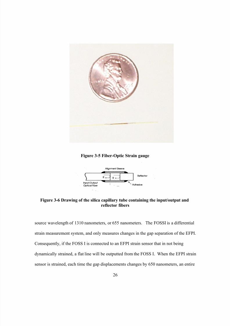
7/28/2019 Weathersby Dis
http://slidepdf.com/reader/full/weathersby-dis 43/280
26
Figure 3-5 Fiber-Optic Strain gauge
Figure 3-6 Drawing of the silica capillary tube containing the input/output and
reflector fibers
source wavelength of 1310 nanometers, or 655 nanometers. The FOSSI is a differential
strain measurement system, and only measures changes in the gap separation of the EFPI.
Consequently, if the FOSS I is connected to an EFPI strain sensor that in not being
dynamically strained, a flat line will be outputted from the FOSS I. When the EFPI strain
sensor is strained, each time the gap displacements changes by 650 nanometers, an entire
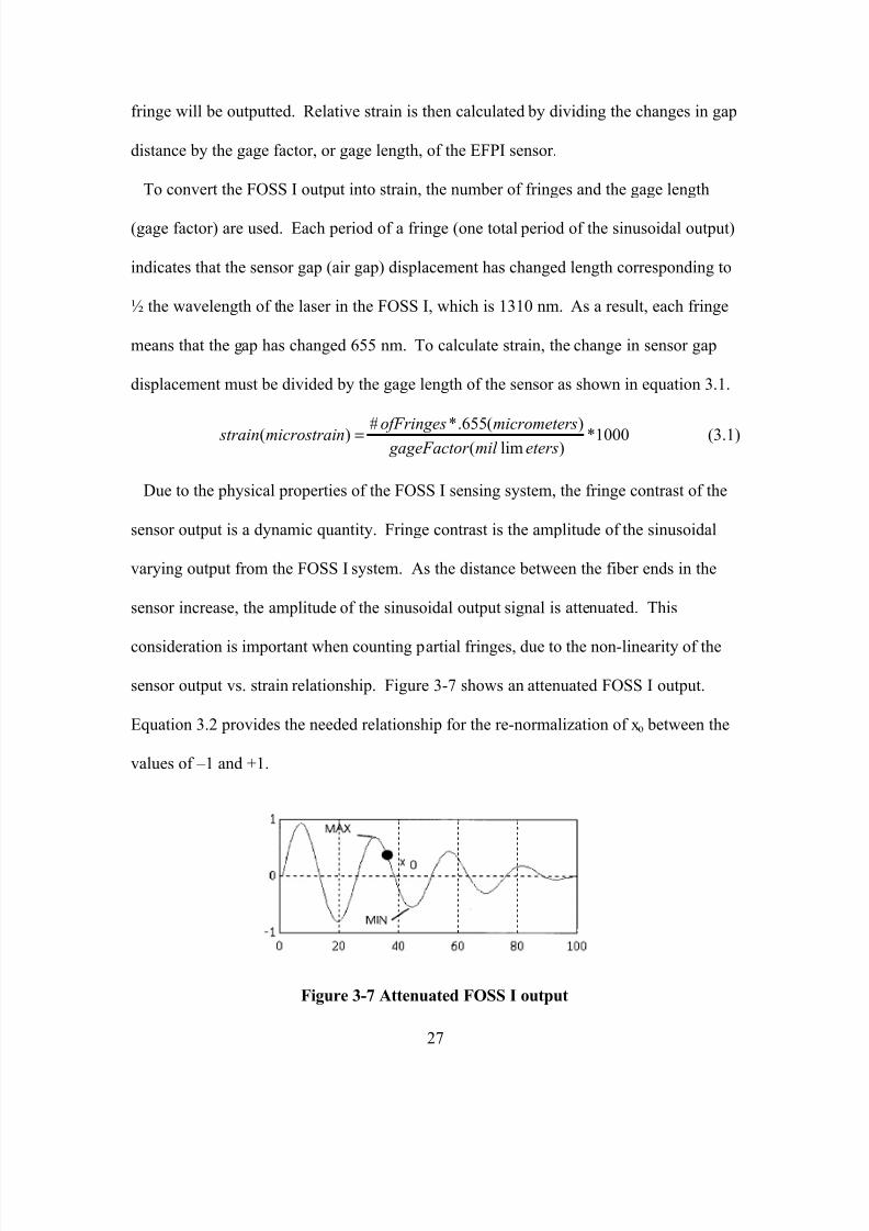
7/28/2019 Weathersby Dis
http://slidepdf.com/reader/full/weathersby-dis 44/280
27
fringe will be outputted. Relative strain is then calculated by dividing the changes in gap
distance by the gage factor, or gage length, of the EFPI sensor.
To convert the FOSS I output into strain, the number of fringes and the gage length
(gage factor) are used. Each period of a fringe (one total period of the sinusoidal output)
indicates that the sensor gap (air gap) displacement has changed length corresponding to
½ the wavelength of the laser in the FOSS I, which is 1310 nm. As a result, each fringe
means that the gap has changed 655 nm. To calculate strain, the change in sensor gap
displacement must be divided by the gage length of the sensor as shown in equation 3.1.
1000*)lim(
)(655.*#)(etersmil gageFactor
smicrometer ofFringesnmicrostrai strain = (3.1)
Due to the physical properties of the FOSS I sensing system, the fringe contrast of the
sensor output is a dynamic quantity. Fringe contrast is the amplitude of the sinusoidal
varying output from the FOSS I system. As the distance between the fiber ends in the
sensor increase, the amplitude of the sinusoidal output signal is attenuated. This
consideration is important when counting partial fringes, due to the non-linearity of the
sensor output vs. strain relationship. Figure 3-7 shows an attenuated FOSS I output.
Equation 3.2 provides the needed relationship for the re-normalization of xo between the
values of –1 and +1.
Figure 3-7 Attenuated FOSS I output
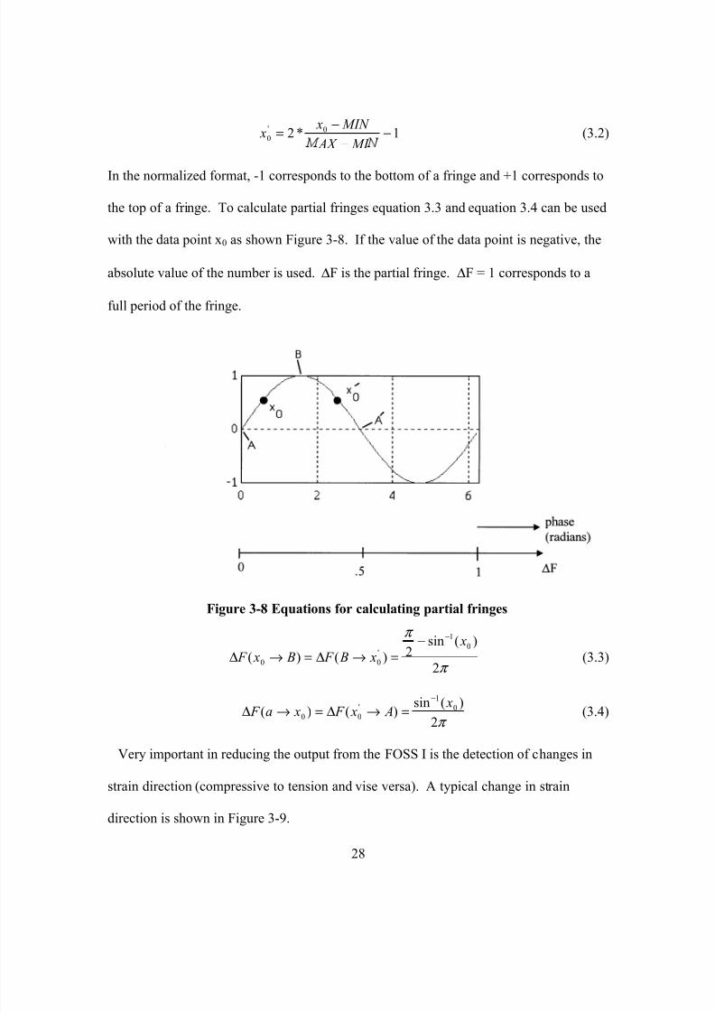
7/28/2019 Weathersby Dis
http://slidepdf.com/reader/full/weathersby-dis 45/280
28
1*2 0'
0 −−
−=
MI AX
MIN x x (3.2)
In the normalized format, -1 corresponds to the bottom of a fringe and +1 corresponds to
the top of a fringe. To calculate partial fringes equation 3.3 and equation 3.4 can be used
with the data point x0 as shown Figure 3-8. If the value of the data point is negative, the
absolute value of the number is used. ∆F is the partial fringe. ∆F = 1 corresponds to a
full period of the fringe.
Figure 3-8 Equations for calculating partial fringes
π
π
2
)(sin2)()(
0
1
'
00
x
x B F B x F
−−=→∆=→∆ (3.3)
π 2)(sin)()( 0
1
'00 x A x F xa F
−
=→∆=→∆ (3.4)
Very important in reducing the output from the FOSS I is the detection of changes in
strain direction (compressive to tension and vise versa). A typical change in strain
direction is shown in Figure 3-9.
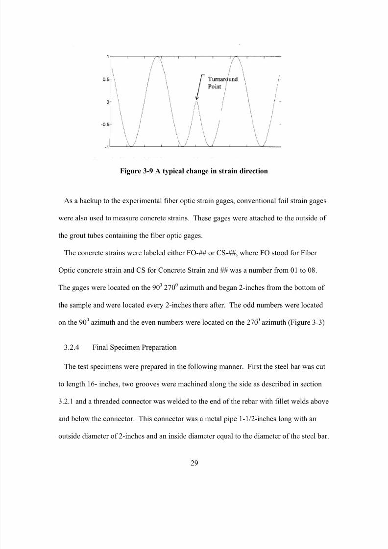
7/28/2019 Weathersby Dis
http://slidepdf.com/reader/full/weathersby-dis 46/280
29
Figure 3-9 A typical change in strain direction
As a backup to the experimental fiber optic strain gages, conventional foil strain gages
were also used to measure concrete strains. These gages were attached to the outside of
the grout tubes containing the fiber optic gages.
The concrete strains were labeled either FO-## or CS-##, where FO stood for Fiber
Optic concrete strain and CS for Concrete Strain and ## was a number from 01 to 08.
The gages were located on the 900
2700
azimuth and began 2-inches from the bottom of
the sample and were located every 2-inches there after. The odd numbers were located
on the 900
azimuth and the even numbers were located on the 2700
azimuth (Figure 3-3)
3.2.4 Final Specimen Preparation
The test specimens were prepared in the following manner. First the steel bar was cut
to length 16- inches, two grooves were machined along the side as described in section
3.2.1 and a threaded connector was welded to the end of the rebar with fillet welds above
and below the connector. This connector was a metal pipe 1-1/2-inches long with an
outside diameter of 2-inches and an inside diameter equal to the diameter of the steel bar.
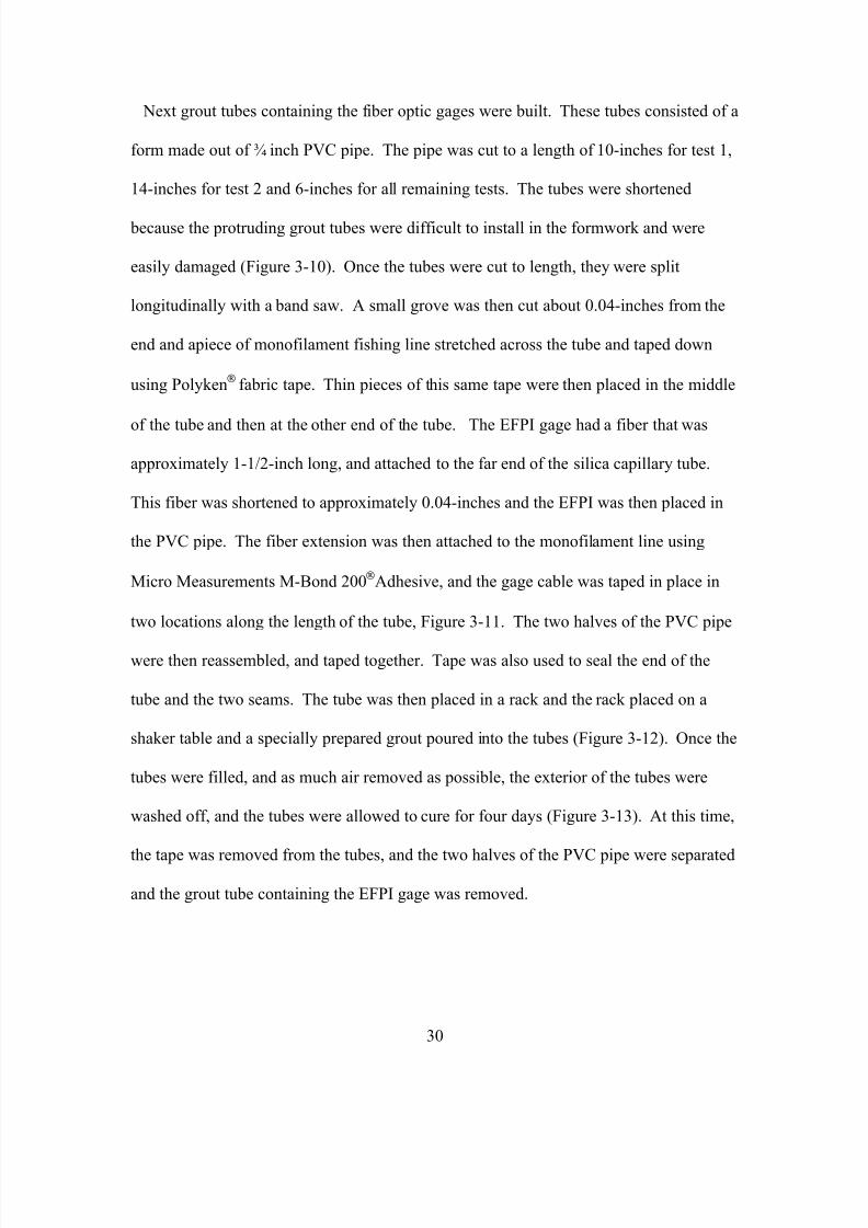
7/28/2019 Weathersby Dis
http://slidepdf.com/reader/full/weathersby-dis 47/280
30
Next grout tubes containing the fiber optic gages were built. These tubes consisted of a
form made out of ¾ inch PVC pipe. The pipe was cut to a length of 10-inches for test 1,
14-inches for test 2 and 6-inches for all remaining tests. The tubes were shortened
because the protruding grout tubes were difficult to install in the formwork and were
easily damaged (Figure 3-10). Once the tubes were cut to length, they were split
longitudinally with a band saw. A small grove was then cut about 0.04-inches from the
end and apiece of monofilament fishing line stretched across the tube and taped down
using Polyken fabric tape. Thin pieces of this same tape were then placed in the middle
of the tube and then at the other end of the tube. The EFPI gage had a fiber that was
approximately 1-1/2-inch long, and attached to the far end of the silica capillary tube.
This fiber was shortened to approximately 0.04-inches and the EFPI was then placed in
the PVC pipe. The fiber extension was then attached to the monofilament line using
Micro Measurements M-Bond 200Adhesive, and the gage cable was taped in place in
two locations along the length of the tube, Figure 3-11. The two halves of the PVC pipe
were then reassembled, and taped together. Tape was also used to seal the end of the
tube and the two seams. The tube was then placed in a rack and the rack placed on a
shaker table and a specially prepared grout poured into the tubes (Figure 3-12). Once the
tubes were filled, and as much air removed as possible, the exterior of the tubes were
washed off, and the tubes were allowed to cure for four days (Figure 3-13). At this time,
the tape was removed from the tubes, and the two halves of the PVC pipe were separated
and the grout tube containing the EFPI gage was removed.
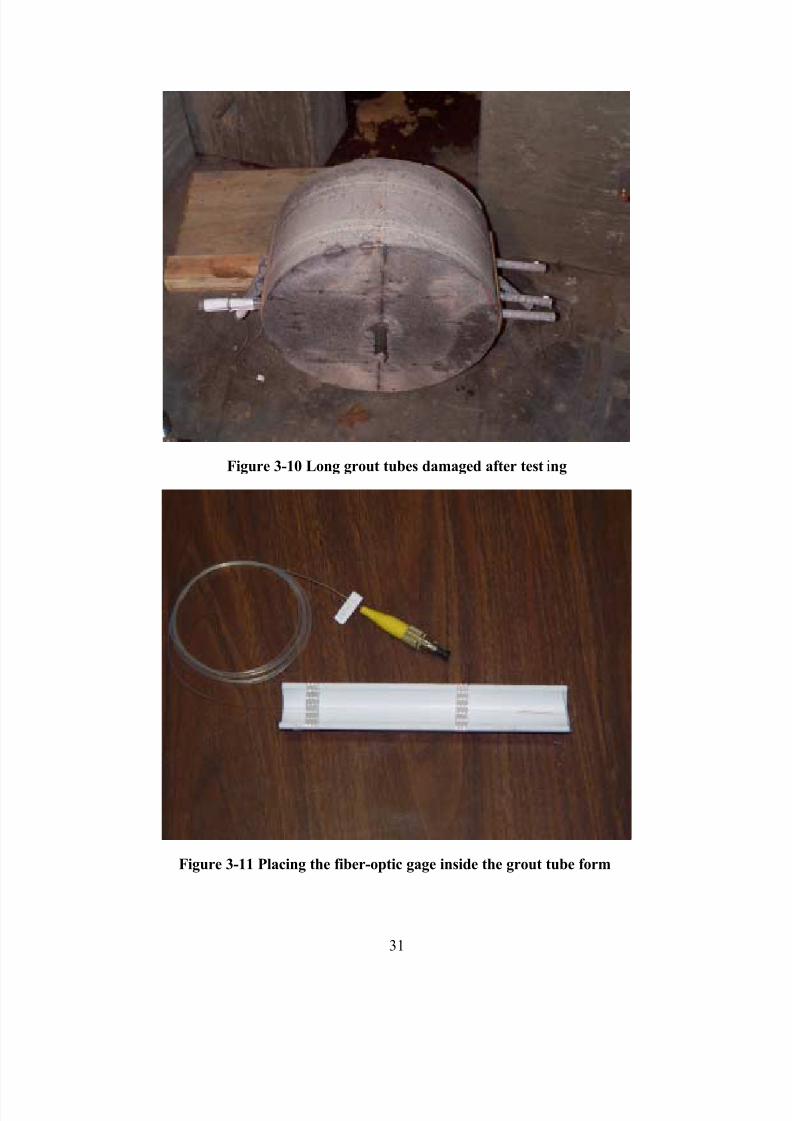
7/28/2019 Weathersby Dis
http://slidepdf.com/reader/full/weathersby-dis 48/280
31
Figure 3-10 Long grout tubes damaged after testing
Figure 3-11 Placing the fiber-optic gage inside the grout tube form
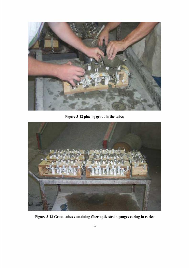
7/28/2019 Weathersby Dis
http://slidepdf.com/reader/full/weathersby-dis 49/280
32
Figure 3-12 placing grout in the tubes
Figure 3-13 Grout tubes containing fiber-optic strain gauges curing in racks
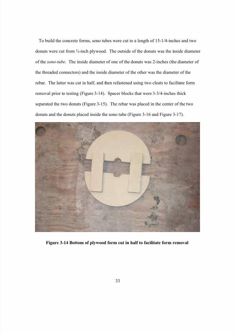
7/28/2019 Weathersby Dis
http://slidepdf.com/reader/full/weathersby-dis 50/280
33
To build the concrete forms, sono tubes were cut to a length of 15-1/4-inches and two
donuts were cut from ¾-inch plywood. The outside of the donuts was the inside diameter
of the sono-tube. The inside diameter of one of the donuts was 2-inches (the diameter of
the threaded connectors) and the inside diameter of the other was the diameter of the
rebar. The latter was cut in half, and then refastened using two cleats to facilitate form
removal prior to testing (Figure 3-14). Spacer blocks that were 3-3/4-inches thick
separated the two donuts (Figure 3-15). The rebar was placed in the center of the two
donuts and the donuts placed inside the sono tube (Figure 3-16 and Figure 3-17).
Figure 3-14 Bottom of plywood form cut in half to facilitate form removal
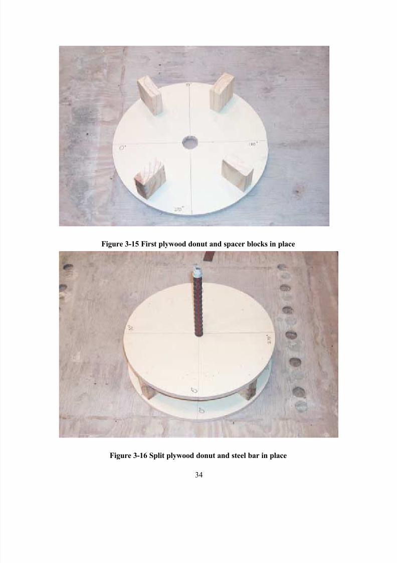
7/28/2019 Weathersby Dis
http://slidepdf.com/reader/full/weathersby-dis 51/280
34
Figure 3-15 First plywood donut and spacer blocks in place
Figure 3-16 Split plywood donut and steel bar in place
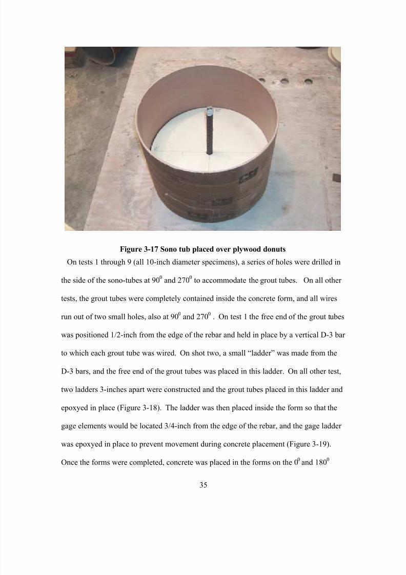
7/28/2019 Weathersby Dis
http://slidepdf.com/reader/full/weathersby-dis 52/280
35
Figure 3-17 Sono tub placed over plywood donuts
On tests 1 through 9 (all 10-inch diameter specimens), a series of holes were drilled in
the side of the sono-tubes at 900
and 2700
to accommodate the grout tubes. On all other
tests, the grout tubes were completely contained inside the concrete form, and all wires
run out of two small holes, also at 900
and 2700
. On test 1 the free end of the grout tubes
was positioned 1/2-inch from the edge of the rebar and held in place by a vertical D-3 bar
to which each grout tube was wired. On shot two, a small “ladder” was made from the
D-3 bars, and the free end of the grout tubes was placed in this ladder. On all other test,
two ladders 3-inches apart were constructed and the grout tubes placed in this ladder and
epoxyed in place (Figure 3-18). The ladder was then placed inside the form so that the
gage elements would be located 3/4-inch from the edge of the rebar, and the gage ladder
was epoxyed in place to prevent movement during concrete placement (Figure 3-19).
Once the forms were completed, concrete was placed in the forms on the 00
and 1800
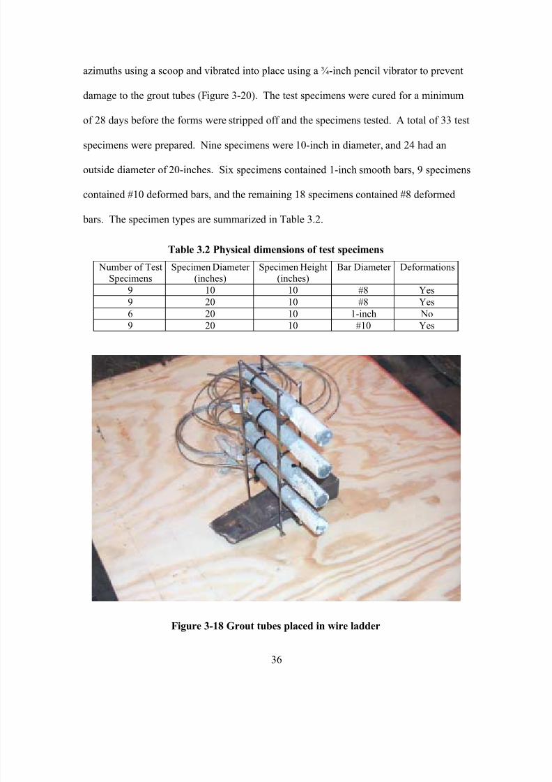
7/28/2019 Weathersby Dis
http://slidepdf.com/reader/full/weathersby-dis 53/280
36
azimuths using a scoop and vibrated into place using a ¾-inch pencil vibrator to prevent
damage to the grout tubes (Figure 3-20). The test specimens were cured for a minimum
of 28 days before the forms were stripped off and the specimens tested. A total of 33 test
specimens were prepared. Nine specimens were 10-inch in diameter, and 24 had an
outside diameter of 20-inches. Six specimens contained 1-inch smooth bars, 9 specimens
contained #10 deformed bars, and the remaining 18 specimens contained #8 deformed
bars. The specimen types are summarized in Table 3.2.
Table 3.2 Physical dimensions of test specimens
Number of TestSpecimens
Specimen Diameter (inches)
Specimen Height(inches)
Bar Diameter Deformations
9 10 10 #8 Yes
9 20 10 #8 Yes
6 20 10 1-inch No
9 20 10 #10 Yes
Figure 3-18 Grout tubes placed in wire ladder
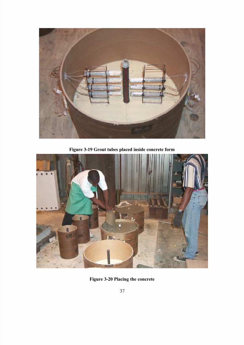
7/28/2019 Weathersby Dis
http://slidepdf.com/reader/full/weathersby-dis 54/280
37
Figure 3-19 Grout tubes placed inside concrete form
Figure 3-20 Placing the concrete
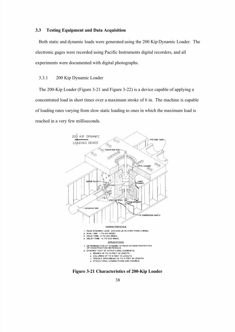
7/28/2019 Weathersby Dis
http://slidepdf.com/reader/full/weathersby-dis 55/280
38
3.3 Testing Equipment and Data Acquisition
Both static and dynamic loads were generated using the 200 Kip Dynamic Loader. The
electronic gages were recorded using Pacific Instruments digital recorders, and all
experiments were documented with digital photographs.
3.3.1 200 Kip Dynamic Loader
The 200-Kip Loader (Figure 3-21 and Figure 3-22) is a device capable of applying a
concentrated load in short times over a maximum stroke of 6 in. The machine is capable
of loading rates varying from slow static loading to ones in which the maximum load is
reached in a very few milliseconds.
Figure 3-21 Characteristics of 200-Kip Loader
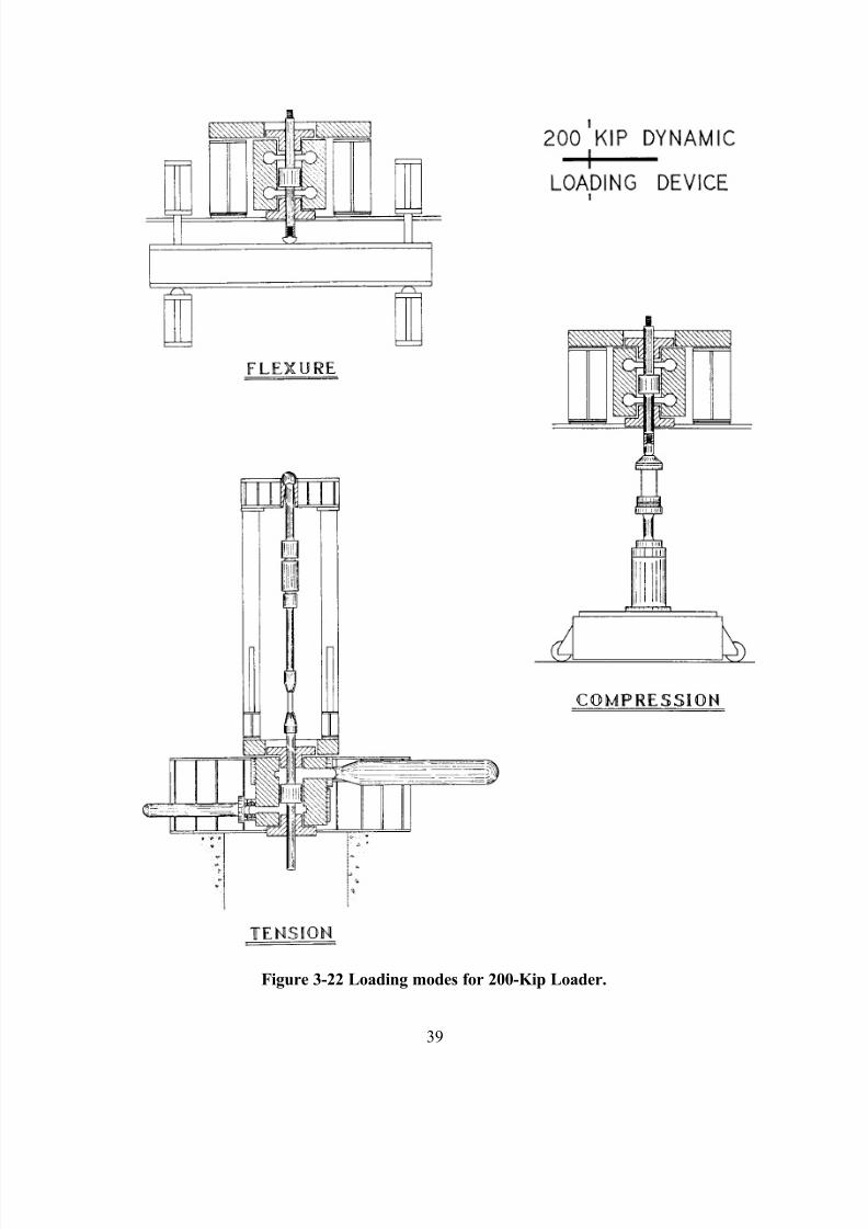
7/28/2019 Weathersby Dis
http://slidepdf.com/reader/full/weathersby-dis 56/280
39
Figure 3-22 Loading modes for 200-Kip Loader.
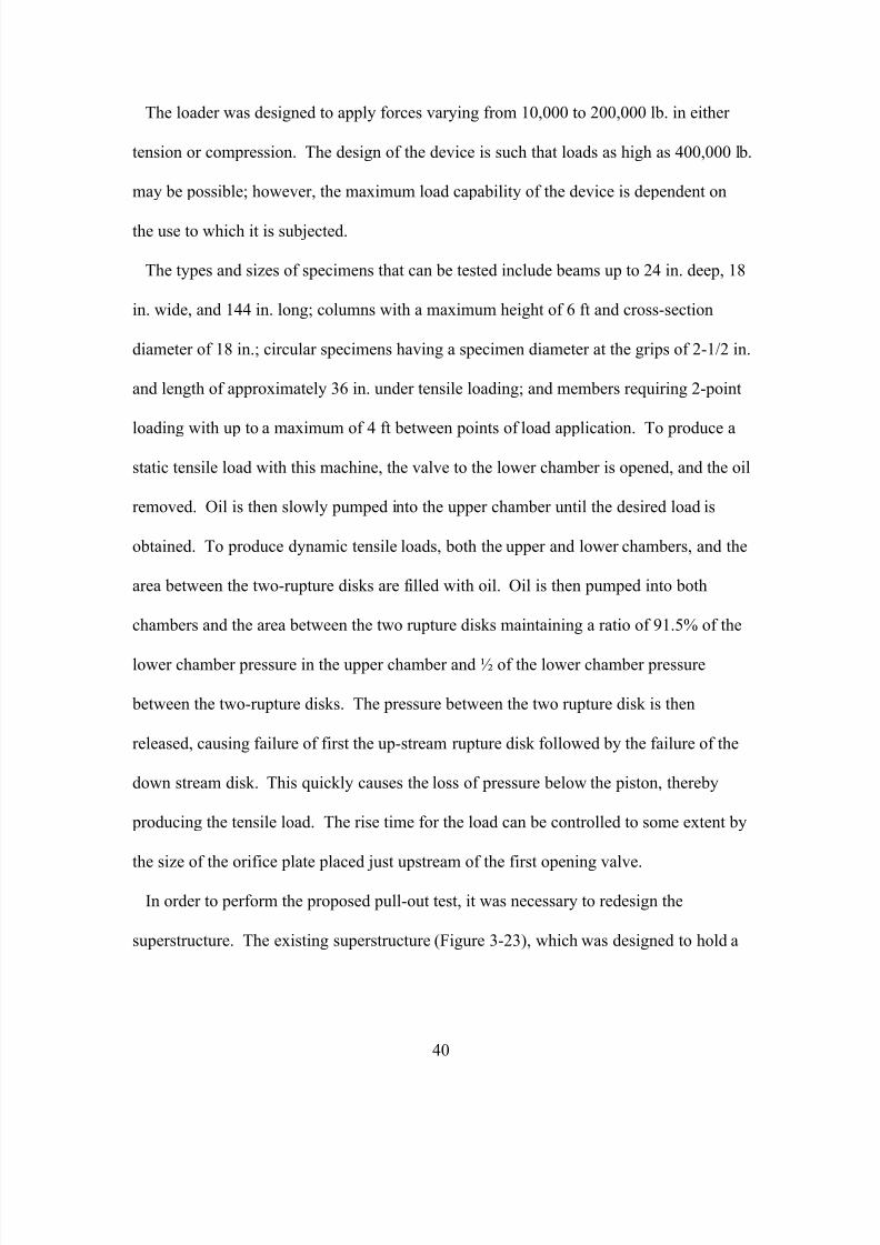
7/28/2019 Weathersby Dis
http://slidepdf.com/reader/full/weathersby-dis 57/280
40
The loader was designed to apply forces varying from 10,000 to 200,000 lb. in either
tension or compression. The design of the device is such that loads as high as 400,000 lb.
may be possible; however, the maximum load capability of the device is dependent on
the use to which it is subjected.
The types and sizes of specimens that can be tested include beams up to 24 in. deep, 18
in. wide, and 144 in. long; columns with a maximum height of 6 ft and cross-section
diameter of 18 in.; circular specimens having a specimen diameter at the grips of 2-1/2 in.
and length of approximately 36 in. under tensile loading; and members requiring 2-point
loading with up to a maximum of 4 ft between points of load application. To produce a
static tensile load with this machine, the valve to the lower chamber is opened, and the oil
removed. Oil is then slowly pumped into the upper chamber until the desired load is
obtained. To produce dynamic tensile loads, both the upper and lower chambers, and the
area between the two-rupture disks are filled with oil. Oil is then pumped into both
chambers and the area between the two rupture disks maintaining a ratio of 91.5% of the
lower chamber pressure in the upper chamber and ½ of the lower chamber pressure
between the two-rupture disks. The pressure between the two rupture disk is then
released, causing failure of first the up-stream rupture disk followed by the failure of the
down stream disk. This quickly causes the loss of pressure below the piston, thereby
producing the tensile load. The rise time for the load can be controlled to some extent by
the size of the orifice plate placed just upstream of the first opening valve.
In order to perform the proposed pull-out test, it was necessary to redesign the
superstructure. The existing superstructure (Figure 3-23), which was designed to hold a
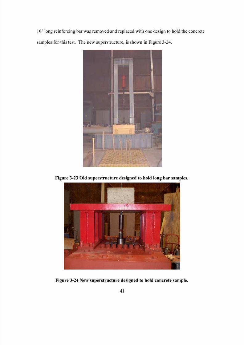
7/28/2019 Weathersby Dis
http://slidepdf.com/reader/full/weathersby-dis 58/280
41
10’ long reinforcing bar was removed and replaced with one design to hold the concrete
samples for this test. The new superstructure, is shown in Figure 3-24.
Figure 3-23 Old superstructure designed to hold long bar samples.
Figure 3-24 New superstructure designed to hold concrete sample.
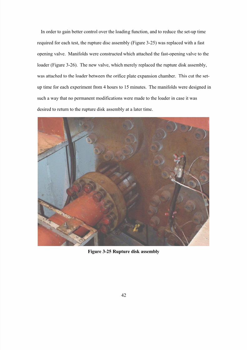
7/28/2019 Weathersby Dis
http://slidepdf.com/reader/full/weathersby-dis 59/280
42
In order to gain better control over the loading function, and to reduce the set-up time
required for each test, the rupture disc assembly (Figure 3-25) was replaced with a fast
opening valve. Manifolds were constructed which attached the fast-opening valve to the
loader (Figure 3-26). The new valve, which merely replaced the rupture disk assembly,
was attached to the loader between the orifice plate expansion chamber. This cut the set-
up time for each experiment from 4 hours to 15 minutes. The manifolds were designed in
such a way that no permanent modifications were made to the loader in case it was
desired to return to the rupture disk assembly at a later time.
Figure 3-25 Rupture disk assembly
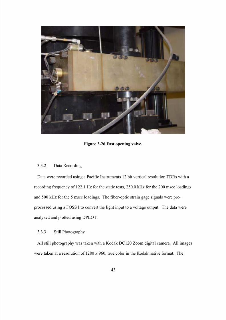
7/28/2019 Weathersby Dis
http://slidepdf.com/reader/full/weathersby-dis 60/280
43
Figure 3-26 Fast opening valve.
3.3.2 Data Recording
Data were recorded using a Pacific Instruments 12 bit vertical resolution TDRs with a
recording frequency of 122.1 Hz for the static tests, 250.0 kHz for the 200 msec loadings
and 500 kHz for the 5 msec loadings. The fiber-optic strain gage signals were pre-
processed using a FOSS I to convert the light input to a voltage output. The data were
analyzed and plotted using DPLOT.
3.3.3 Still Photography
All still photography was taken with a Kodak DC120 Zoom digital camera. All images
were taken at a resolution of 1280 x 960, true color in the Kodak native format. The
7/28/2019 Weathersby Dis
http://slidepdf.com/reader/full/weathersby-dis 61/280
44
images were then converted to tiff format, 256 colors, using Adobe PhotoShop, so the
images could be manipulated using MS word and MS Power Point software.
3.4 Testing Program
The testing program was designed to quantitatively investigate the phenomenon
associated with the interaction of reinforcement and concrete when subjected to a variety
of loading rates, and determine the effects that several parameters had on this interaction.
This would then be followed by a finite element analysis to gain a better understanding of
the physics behind this relationship.
3.4.1 Test Matrix
A total of thirty-three specimens were prepared. The baseline specimens consisted of a
#8 deformed bar cast in the center of a 20-inch diameter concrete cylinder. Nine of these
specimens were fabricated and tested. Three were loaded statically, three were loaded in
200 msec, and three were loaded to failure in approximately 5 msec. Three other
variables were investigated. These included: effects of concrete confinement, (i.e., 20-
inch diameter samples vs. 10-inch diameter samples); effects of bar diameter, (i.e., #8
deformed bar vs. #10 deformed bar); and the effects of bar deformation, (i.e., #8
deformed bar vs. 1-inch smooth bar). In each case multiple samples were loaded to
failure statically, in 200 msec and in 5 msec. For each variable and loading rate
combination, three samples were tested, except for the smooth bars where only two were
tested for each loading rate. This was done in order to determine the repeatability of the
experiments, and to obtain a better statistical basis for the data. The complete test matrix
is shown in Table 3.3
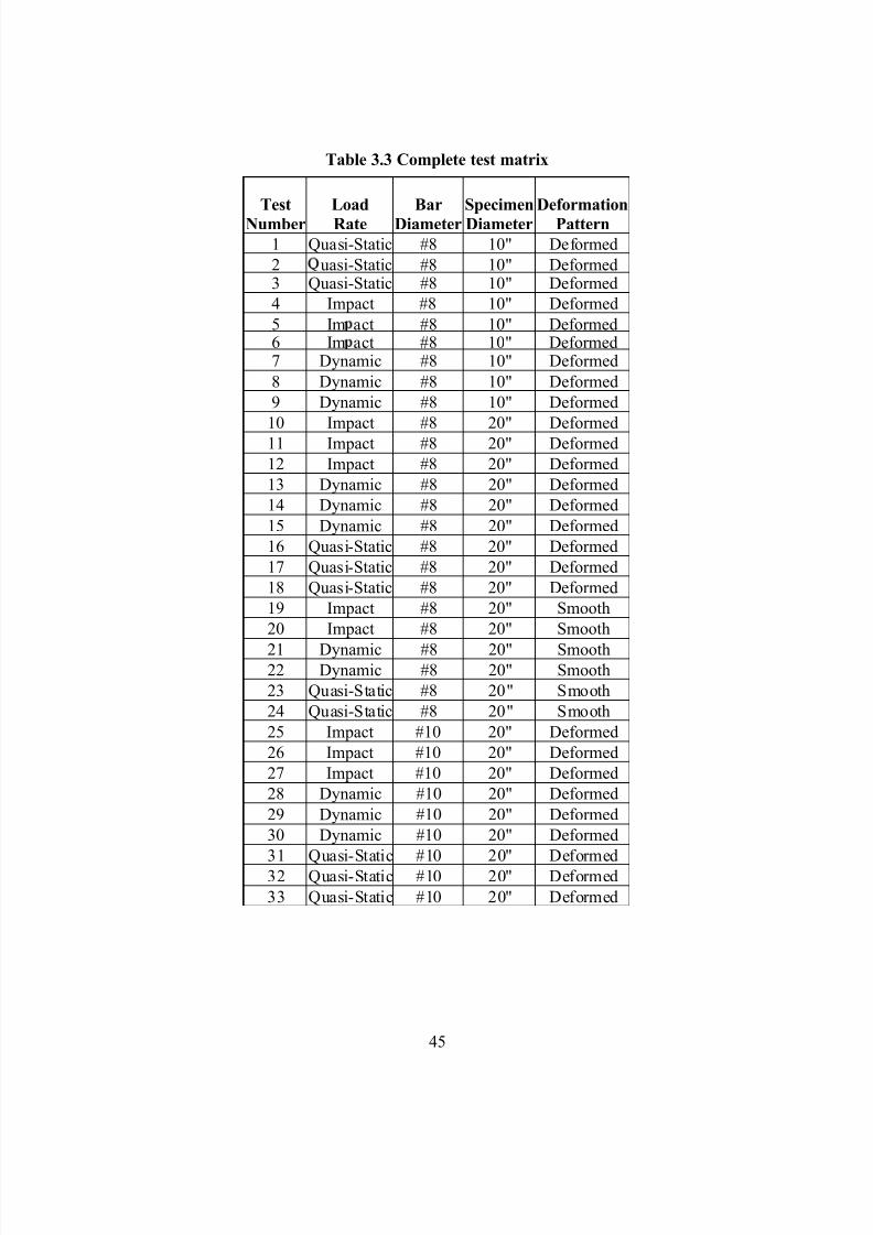
7/28/2019 Weathersby Dis
http://slidepdf.com/reader/full/weathersby-dis 62/280
45
Table 3.3 Complete test matrix
Test
Number
Load
Rate
Bar
Diameter
Specimen
Diameter
Deformation
Pattern
1 Quasi-Static #8 10" Deformed
2 uasi-Static #8 10" Deformed3 Quasi-Static #8 10" Deformed
4 Impact #8 10" Deformed
5 Im act #8 10" Deformed6 Im act #8 10" Deformed7 Dynamic #8 10" Deformed
8 Dynamic #8 10" Deformed
9 Dynamic #8 10" Deformed
10 Impact #8 20" Deformed
11 Impact #8 20" Deformed
12 Impact #8 20" Deformed
13 Dynamic #8 20" Deformed
14 Dynamic #8 20" Deformed
15 Dynamic #8 20" Deformed
16 Quasi-Static #8 20" Deformed
17 Quasi-Static #8 20" Deformed
18 Quasi-Static #8 20" Deformed
19 Impact #8 20" Smooth
20 Impact #8 20" Smooth
21 Dynamic #8 20" Smooth22 Dynamic #8 20" Smooth
23 Quasi-Static #8 20" Smooth
24 Quasi-Static #8 20" Smooth
25 Impact #10 20" Deformed
26 Impact #10 20" Deformed
27 Impact #10 20" Deformed
28 Dynamic #10 20" Deformed
29 Dynamic #10 20" Deformed
30 Dynamic #10 20" Deformed
31 Quasi-Static #10 20" Deformed
32 Quasi-Static #10 20" Deformed
33 Quasi-Static #10 20" Deformed
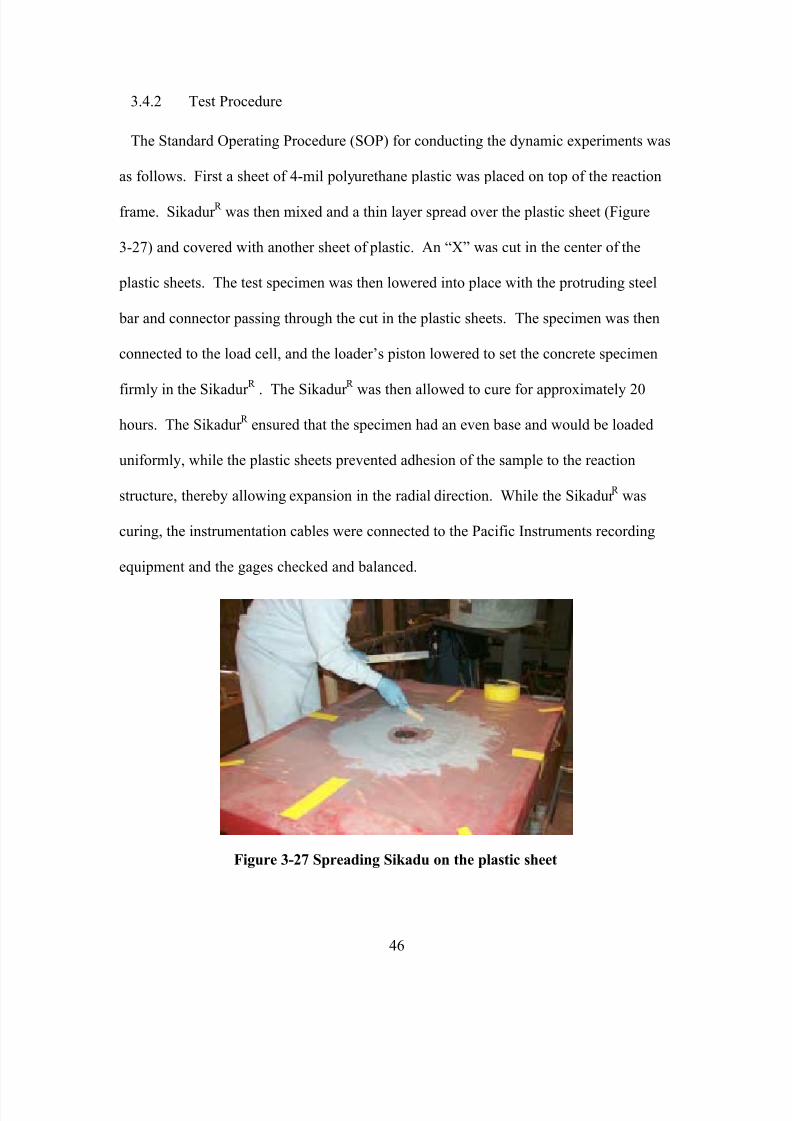
7/28/2019 Weathersby Dis
http://slidepdf.com/reader/full/weathersby-dis 63/280
46
3.4.2 Test Procedure
The Standard Operating Procedure (SOP) for conducting the dynamic experiments was
as follows. First a sheet of 4-mil polyurethane plastic was placed on top of the reaction
frame. Sikadur R
was then mixed and a thin layer spread over the plastic sheet (Figure
3-27) and covered with another sheet of plastic. An “X” was cut in the center of the
plastic sheets. The test specimen was then lowered into place with the protruding steel
bar and connector passing through the cut in the plastic sheets. The specimen was then
connected to the load cell, and the loader’s piston lowered to set the concrete specimen
firmly in the Sikadur R
. The Sikadur R
was then allowed to cure for approximately 20
hours. The Sikadur R
ensured that the specimen had an even base and would be loaded
uniformly, while the plastic sheets prevented adhesion of the sample to the reaction
structure, thereby allowing expansion in the radial direction. While the Sikadur R
was
curing, the instrumentation cables were connected to the Pacific Instruments recording
equipment and the gages checked and balanced.
Figure 3-27 Spreading Sikadu on the plastic sheet
7/28/2019 Weathersby Dis
http://slidepdf.com/reader/full/weathersby-dis 64/280
47
When the Sikadur R
was completely cured, the fast opening valve was tested to ensure
proper function, and the upper and lower cylinders of the loader were bled to remove and
entrapped air bubbles. The piston control valve was then cycled to ensure that no loads
were being applied to the specimen. The load cell output was then set to zero and the
low-pressure valves on the loader closed. The high-pressure hydraulic pump was then
started, and the valve to the upper cylinder opened. The valve to the lower cylinder was
then opened and closed as necessary to maintain zero load on the test specimen.
When the prescribed hydraulic pressure had been obtained, 2250 psi for 200 msec
loadings and 3000 psi for 5 msec loadings, all valves closed, and the pump shut off.
When the instrumentation personnel indicated that they were ready, a 5 second count
down commenced. The fast opening valve was armed at T-4 seconds, the
instrumentation system was armed at T-3 seconds and the fast opening valve was fired a
T=0.
Immediately following the test, the data records were transferred from the systems
RAM to the hard drive. Once this critical stage had been completed, the test specimen
was photographed and removed, the expansion chamber drained, and the loader prepared
for the next experiment.
The SOP for the static tests was identical to the dynamic test except for the loading
stage. Once the system had been bled and the lower pressure valves closed, the fast
opening valve was opened. Oil was then pumped into the upper cylinder while zero
pressure was maintained in the lower cylinder. The loading was continued until the
specimen failed. The remainder of the procedure was the same.
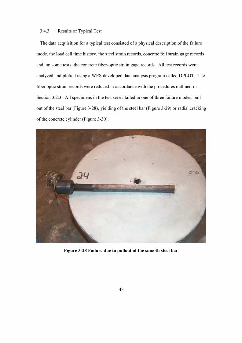
7/28/2019 Weathersby Dis
http://slidepdf.com/reader/full/weathersby-dis 65/280
48
3.4.3 Results of Typical Test
The data acquisition for a typical test consisted of a physical description of the failure
mode, the load cell time history, the steel strain records, concrete foil strain gage records
and, on some tests, the concrete fiber-optic strain gage records. All test records were
analyzed and plotted using a WES developed data analysis program called DPLOT. The
fiber optic strain records were reduced in accordance with the procedures outlined in
Section 3.2.3. All specimens in the test series failed in one of three failure modes; pull
out of the steel bar (Figure 3-28), yielding of the steel bar (Figure 3-29) or radial cracking
of the concrete cylinder (Figure 3-30).
Figure 3-28 Failure due to pullout of the smooth steel bar
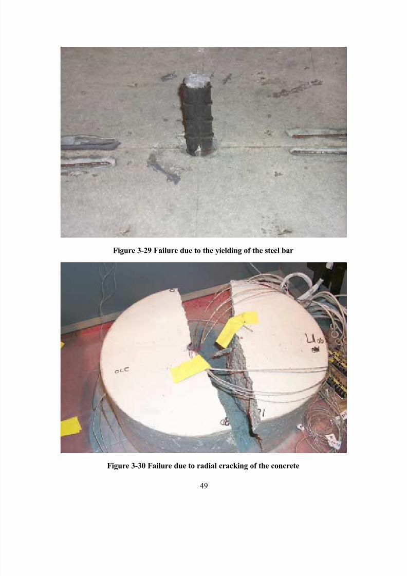
7/28/2019 Weathersby Dis
http://slidepdf.com/reader/full/weathersby-dis 66/280
49
Figure 3-29 Failure due to the yielding of the steel bar
Figure 3-30 Failure due to radial cracking of the concrete
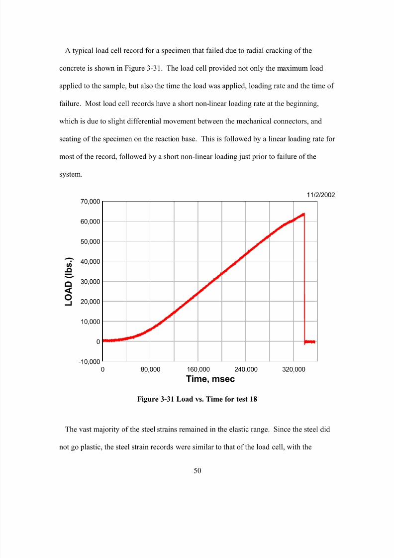
7/28/2019 Weathersby Dis
http://slidepdf.com/reader/full/weathersby-dis 67/280
50
A typical load cell record for a specimen that failed due to radial cracking of the
concrete is shown in Figure 3-31. The load cell provided not only the maximum load
applied to the sample, but also the time the load was applied, loading rate and the time of
failure. Most load cell records have a short non-linear loading rate at the beginning,
which is due to slight differential movement between the mechanical connectors, and
seating of the specimen on the reaction base. This is followed by a linear loading rate for
most of the record, followed by a short non-linear loading just prior to failure of the
system.
11/2/2002
Time, msec
L O A
D ( l b s . )
0 80,000 160,000 240,000 320,000-10,000
0
10,000
20,000
30,000
40,000
50,000
60,000
70,000
Figure 3-31 Load vs. Time for test 18
The vast majority of the steel strains remained in the elastic range. Since the steel did
not go plastic, the steel strain records were similar to that of the load cell, with the
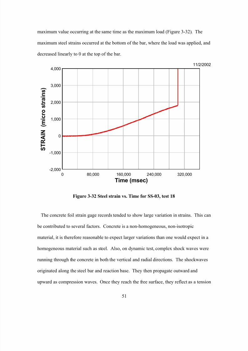
7/28/2019 Weathersby Dis
http://slidepdf.com/reader/full/weathersby-dis 68/280
51
maximum value occurring at the same time as the maximum load (Figure 3-32). The
maximum steel strains occurred at the bottom of the bar, where the load was applied, and
decreased linearly to 0 at the top of the bar.
11/2/2002
Time (msec)
S T R A I N
( m
i c r o s t r a i n s )
0 80,000 160,000 240,000 320,000-2,000
-1,000
0
1,000
2,000
3,000
4,000
Figure 3-32 Steel strain vs. Time for SS-03, test 18
The concrete foil strain gage records tended to show large variation in strains. This can
be contributed to several factors. Concrete is a non-homogeneous, non-isotropic
material, it is therefore reasonable to expect larger variations than one would expect in a
homogeneous material such as steel. Also, on dynamic test, complex shock waves were
running through the concrete in both the vertical and radial directions. The shockwaves
originated along the steel bar and reaction base. They then propagate outward and
upward as compression waves. Once they reach the free surface, they reflect as a tension
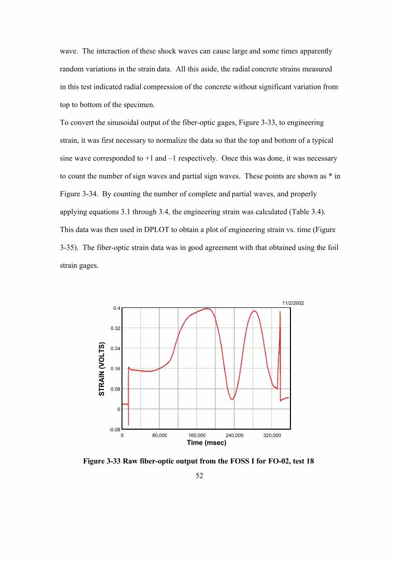
7/28/2019 Weathersby Dis
http://slidepdf.com/reader/full/weathersby-dis 69/280
52
wave. The interaction of these shock waves can cause large and some times apparently
random variations in the strain data. All this aside, the radial concrete strains measured
in this test indicated radial compression of the concrete without significant variation from
top to bottom of the specimen.
To convert the sinusoidal output of the fiber-optic gages, Figure 3-33, to engineering
strain, it was first necessary to normalize the data so that the top and bottom of a typical
sine wave corresponded to +1 and –1 respectively. Once this was done, it was necessary
to count the number of sign waves and partial sign waves. These points are shown as * in
Figure 3-34. By counting the number of complete and partial waves, and properly
applying equations 3.1 through 3.4, the engineering strain was calculated (Table 3.4).
This data was then used in DPLOT to obtain a plot of engineering strain vs. time (Figure
3-35). The fiber-optic strain data was in good agreement with that obtained using the foil
strain gages.
11/2/2002
Time (msec)
S
T R A I N ( V O L T S )
0 80,000 160,000 240,000 320,000-0.08
0
0.08
0.16
0.24
0.32
0.4
Figure 3-33 Raw fiber-optic output from the FOSS I for FO-02, test 18
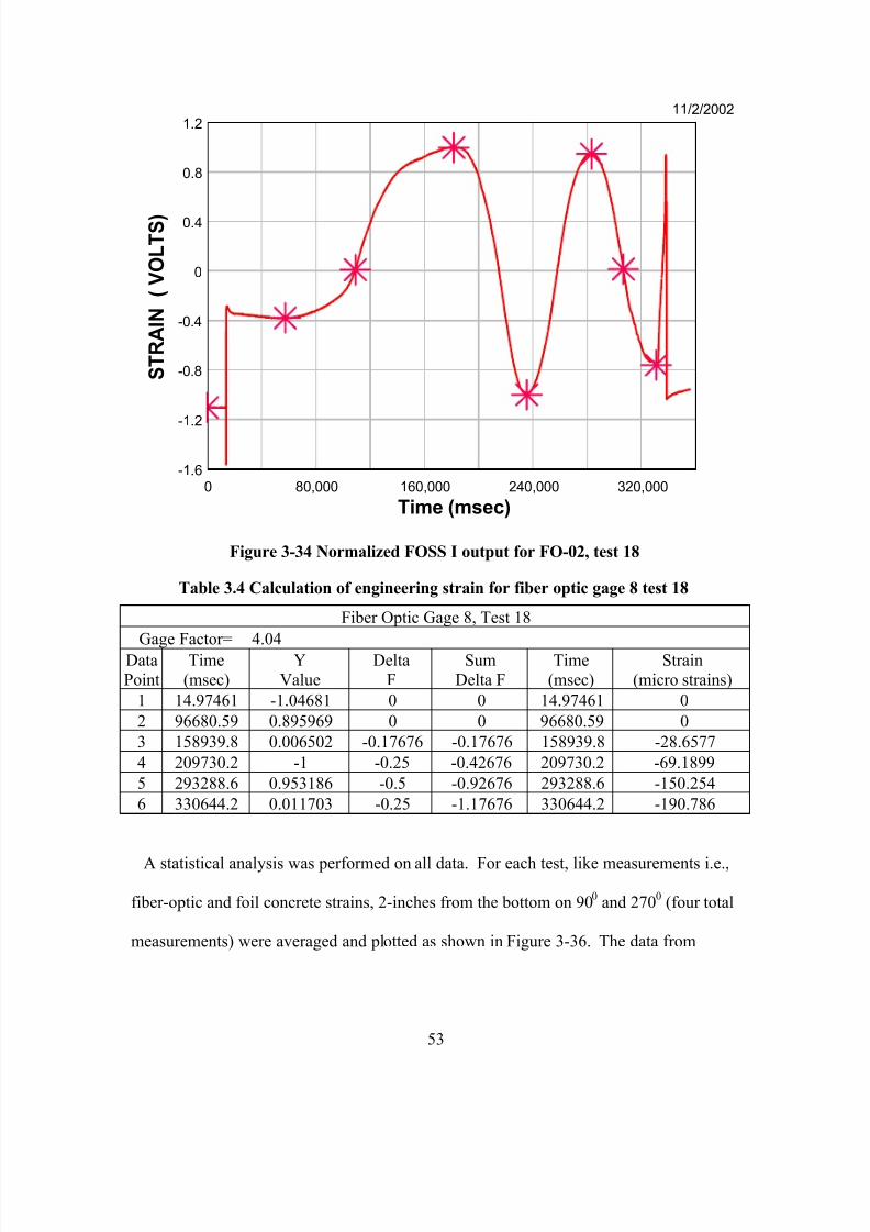
7/28/2019 Weathersby Dis
http://slidepdf.com/reader/full/weathersby-dis 70/280
53
11/2/2002
Time (msec)
S T R A I N
( V O L T S )
0 80,000 160,000 240,000 320,000-1.6
-1.2
-0.8
-0.4
0
0.4
0.8
1.2
Figure 3-34 Normalized FOSS I output for FO-02, test 18
Table 3.4 Calculation of engineering strain for fiber optic gage 8 test 18
Fiber Optic Gage 8, Test 18
Gage Factor= 4.04Data
Point
Time
(msec)
Y
Value
Delta
F
Sum
Delta F
Time
(msec)
Strain
(micro strains)
1 14.97461 -1.04681 0 0 14.97461 0
2 96680.59 0.895969 0 0 96680.59 0
3 158939.8 0.006502 -0.17676 -0.17676 158939.8 -28.6577
4 209730.2 -1 -0.25 -0.42676 209730.2 -69.1899
5 293288.6 0.953186 -0.5 -0.92676 293288.6 -150.254
6 330644.2 0.011703 -0.25 -1.17676 330644.2 -190.786
A statistical analysis was performed on all data. For each test, like measurements i.e.,
fiber-optic and foil concrete strains, 2-inches from the bottom on 900
and 2700
(four total
measurements) were averaged and plotted as shown in Figure 3-36. The data from
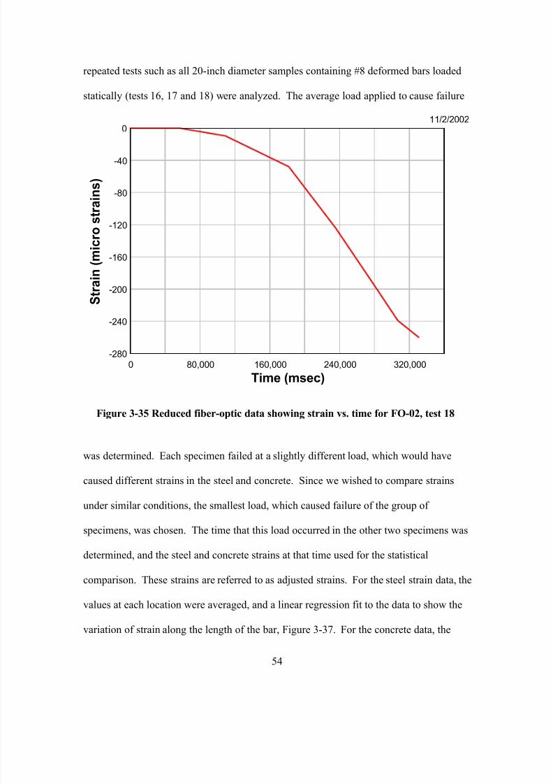
7/28/2019 Weathersby Dis
http://slidepdf.com/reader/full/weathersby-dis 71/280
54
repeated tests such as all 20-inch diameter samples containing #8 deformed bars loaded
statically (tests 16, 17 and 18) were analyzed. The average load applied to cause failure
11/2/2002
Time (msec)
S t r a i n
( m i c r o s t r a i n s )
0 80,000 160,000 240,000 320,000-280
-240
-200
-160
-120
-80
-40
0
Figure 3-35 Reduced fiber-optic data showing strain vs. time for FO-02, test 18
was determined. Each specimen failed at a slightly different load, which would have
caused different strains in the steel and concrete. Since we wished to compare strains
under similar conditions, the smallest load, which caused failure of the group of
specimens, was chosen. The time that this load occurred in the other two specimens was
determined, and the steel and concrete strains at that time used for the statistical
comparison. These strains are referred to as adjusted strains. For the steel strain data, the
values at each location were averaged, and a linear regression fit to the data to show the
variation of strain along the length of the bar, Figure 3-37. For the concrete data, the
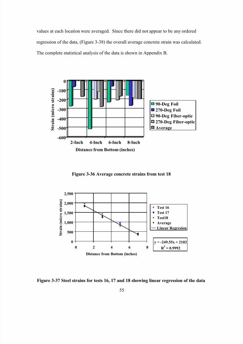
7/28/2019 Weathersby Dis
http://slidepdf.com/reader/full/weathersby-dis 72/280
55
values at each location were averaged. Since there did not appear to be any ordered
regression of the data, (Figure 3-38) the overall average concrete strain was calculated.
The complete statistical analysis of the data is shown in Appendix B.
Figure 3-36 Average concrete strains from test 18
y = -249.55x + 2102
R 2
= 0.9992
0
500
1,000
1,500
2,000
2,500
0 2 4 6 8
Distance from Bottom (inches)
S t r a i n ( m i c r o s t r a i n s )
Test 16
Test 17
Test18
Average
Linear Regresion
Figure 3-37 Steel strains for tests 16, 17 and 18 showing linear regression of the data
-600
-500
-400
-300
-200
-100
0
S t r a i n
( m i c r o s t r a i n s )
2-Inch 4-Inch 6-Inch 8-Inch
Distance from Bottom (inches)
90-Deg Foil
270-Deg Foil
90-Deg Fiber-optic
270-Deg Fiber-optic
Average
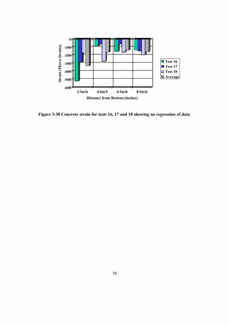
7/28/2019 Weathersby Dis
http://slidepdf.com/reader/full/weathersby-dis 73/280
56
-600
-500
-400
-300
-200
-100
0
S t r a i n ( M i c r o S t r a i n s )
2-Inch 4-Inch 6-Inch 8-Inch
Distance from Bottom (inches)
Test 16
Test 17
Test 18
Average
Figure 3-38 Concrete strain for tests 16, 17 and 18 showing no regression of data
7/28/2019 Weathersby Dis
http://slidepdf.com/reader/full/weathersby-dis 74/280
57
CHAPTER 4 EXPERIMENTAL RESULTS
This chapter presents the actual test data obtained from each test. A series of three
similar tests were conducted for each variable. Since failure for each specimen occurred
at slightly different loads, the smallest load that caused failure in the group was used as
the maximum load. The time that this load occurred in the other two tests was
determined, and the strain values at that time used in the comparisons. A complete
summary including post test pictures of the specimens, Summary graphs of the steel
strains and concrete strains for each test, and a statistical analysis of the data can be found
in Appendix B.
4.1 Quasi-Static Loading of a #8 Deformed Bar Embedded in a 10-inch Diameter
Concrete Cylinder
Tests 1, 2 and 3 consisted of a 10-inch diameter cylinder with a #8 deformed bar loaded
quasi-statically. Oil was pumped into the upper cylinder of the machine to create the
loads applied to the specimens. The rate at which the loads were applied was a function
of the rate that the oil was pumped. This could be affected by many variables such as the
manifold pressure or the temperature of the oil. The loads applied to each specimen were
slowly increased until failure occurred. The maximum loads applied to the three test
specimens before failure were 41,000 lbs. at time t = 417 sec. For test 1, 40,300 lbs. at t =
240 sec. for test 2 and 42,580 lbs. at t = 713 sec. Since these were all quasi-static tests,
the differences in time had no effect on the results. In order to compare all data under
comparable loading conditions, a maximum load of 40,300 lbs. will be used for these
three tests.
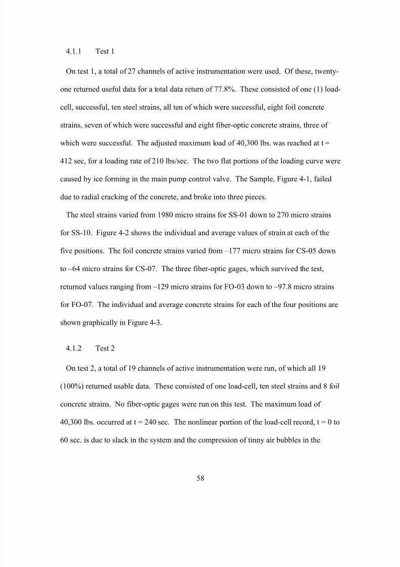
7/28/2019 Weathersby Dis
http://slidepdf.com/reader/full/weathersby-dis 75/280
58
4.1.1 Test 1
On test 1, a total of 27 channels of active instrumentation were used. Of these, twenty-
one returned useful data for a total data return of 77.8%. These consisted of one (1) load-
cell, successful, ten steel strains, all ten of which were successful, eight foil concrete
strains, seven of which were successful and eight fiber-optic concrete strains, three of
which were successful. The adjusted maximum load of 40,300 lbs. was reached at t =
412 sec, for a loading rate of 210 lbs/sec. The two flat portions of the loading curve were
caused by ice forming in the main pump control valve. The Sample, Figure 4-1, failed
due to radial cracking of the concrete, and broke into three pieces.
The steel strains varied from 1980 micro strains for SS-01 down to 270 micro strains
for SS-10. Figure 4-2 shows the individual and average values of strain at each of the
five positions. The foil concrete strains varied from –177 micro strains for CS-05 down
to –64 micro strains for CS-07. The three fiber-optic gages, which survived the test,
returned values ranging from –129 micro strains for FO-03 down to –97.8 micro strains
for FO-07. The individual and average concrete strains for each of the four positions are
shown graphically in Figure 4-3.
4.1.2 Test 2
On test 2, a total of 19 channels of active instrumentation were run, of which all 19
(100%) returned usable data. These consisted of one load-cell, ten steel strains and 8 foil
concrete strains. No fiber-optic gages were run on this test. The maximum load of
40,300 lbs. occurred at t = 240 sec. The nonlinear portion of the load-cell record, t = 0 to
60 sec. is due to slack in the system and the compression of tinny air bubbles in the
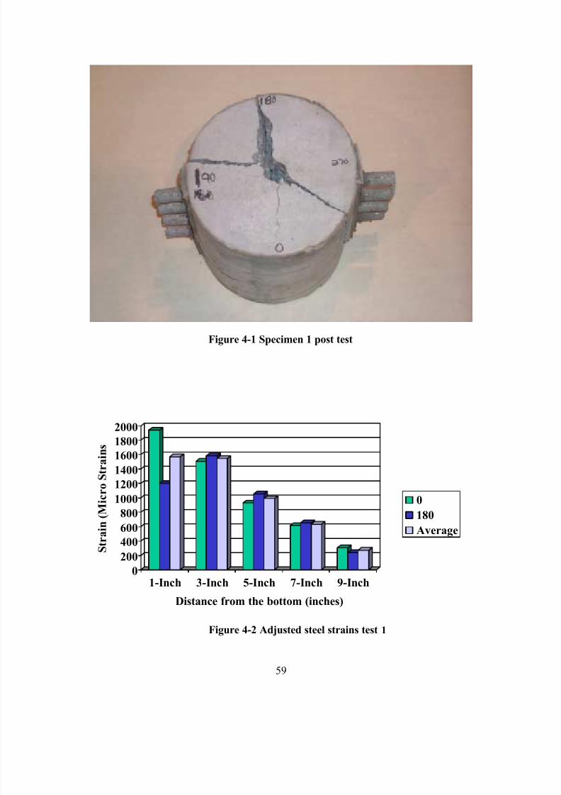
7/28/2019 Weathersby Dis
http://slidepdf.com/reader/full/weathersby-dis 76/280
59
Figure 4-1 Specimen 1 post test
0200
400
600
800
1000
1200
1400
1600
1800
2000
S t r a i n ( M i c r o S t r a i n s
1-Inch 3-Inch 5-Inch 7-Inch 9-Inch
Distance from the bottom (inches)
0
180
Average
Figure 4-2 Adjusted steel strains test 1
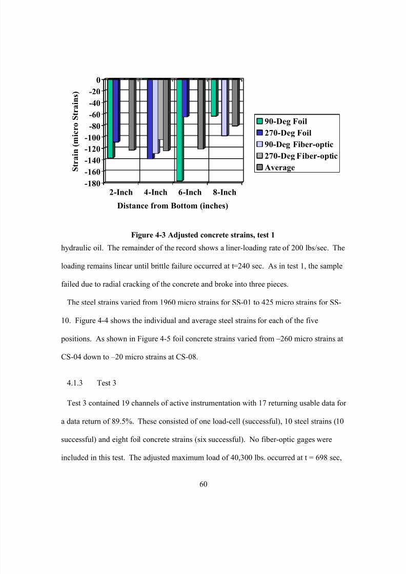
7/28/2019 Weathersby Dis
http://slidepdf.com/reader/full/weathersby-dis 77/280
60
-180
-160
-140
-120
-100
-80
-60
-40
-20
0
S t r a i n ( m i c r o S t r a i n
s )
2-Inch 4-Inch 6-Inch 8-Inch
Distance from Bottom (inches)
90-Deg Foil
270-Deg Foil
90-Deg Fiber-optic
270-Deg Fiber-optic
Average
Figure 4-3 Adjusted concrete strains, test 1
hydraulic oil. The remainder of the record shows a liner-loading rate of 200 lbs/sec. The
loading remains linear until brittle failure occurred at t=240 sec. As in test 1, the sample
failed due to radial cracking of the concrete and broke into three pieces.
The steel strains varied from 1960 micro strains for SS-01 to 425 micro strains for SS-
10. Figure 4-4 shows the individual and average steel strains for each of the five
positions. As shown in Figure 4-5 foil concrete strains varied from –260 micro strains at
CS-04 down to –20 micro strains at CS-08.
4.1.3 Test 3
Test 3 contained 19 channels of active instrumentation with 17 returning usable data for
a data return of 89.5%. These consisted of one load-cell (successful), 10 steel strains (10
successful) and eight foil concrete strains (six successful). No fiber-optic gages were
included in this test. The adjusted maximum load of 40,300 lbs. occurred at t = 698 sec,
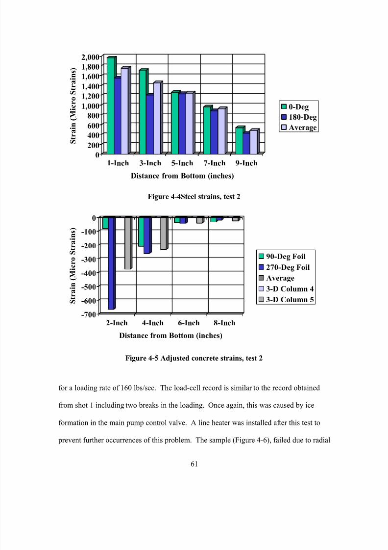
7/28/2019 Weathersby Dis
http://slidepdf.com/reader/full/weathersby-dis 78/280
61
0
200
400
600
800
1,0001,200
1,400
1,600
1,800
2,000
S t r a i n ( M i c r o S t r a i n s )
1-Inch 3-Inch 5-Inch 7-Inch 9-Inch
Distance from Bottom (inches)
0-Deg
180-Deg
Average
Figure 4-4Steel strains, test 2
-700
-600
-500
-400
-300
-200
-100
0
S t r a i
n ( M i c r o S t r a i n s )
2-Inch 4-Inch 6-Inch 8-Inch
Distance from Bottom (inches)
90-Deg Foil
270-Deg Foil
Average
3-D Column 43-D Column 5
Figure 4-5 Adjusted concrete strains, test 2
for a loading rate of 160 lbs/sec. The load-cell record is similar to the record obtained
from shot 1 including two breaks in the loading. Once again, this was caused by ice
formation in the main pump control valve. A line heater was installed after this test to
prevent further occurrences of this problem. The sample (Figure 4-6), failed due to radial
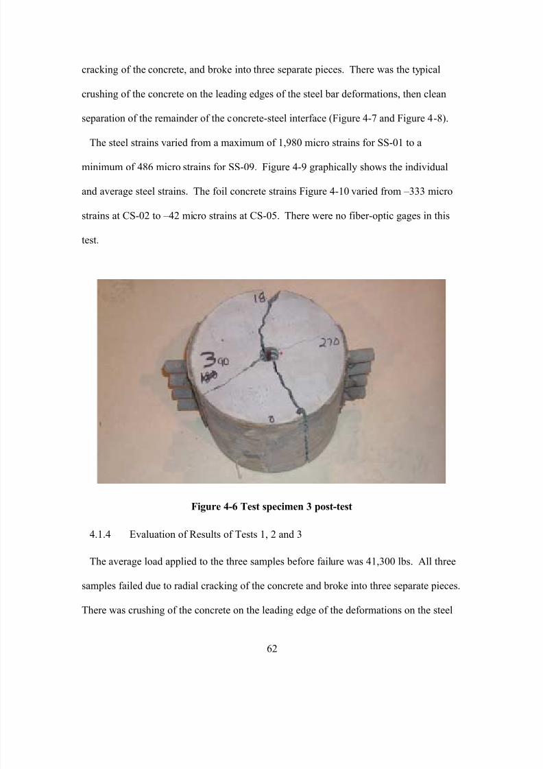
7/28/2019 Weathersby Dis
http://slidepdf.com/reader/full/weathersby-dis 79/280
62
cracking of the concrete, and broke into three separate pieces. There was the typical
crushing of the concrete on the leading edges of the steel bar deformations, then clean
separation of the remainder of the concrete-steel interface (Figure 4-7 and Figure 4-8).
The steel strains varied from a maximum of 1,980 micro strains for SS-01 to a
minimum of 486 micro strains for SS-09. Figure 4-9 graphically shows the individual
and average steel strains. The foil concrete strains Figure 4-10 varied from –333 micro
strains at CS-02 to –42 micro strains at CS-05. There were no fiber-optic gages in this
test.
Figure 4-6 Test specimen 3 post-test
4.1.4 Evaluation of Results of Tests 1, 2 and 3
The average load applied to the three samples before failure was 41,300 lbs. All three
samples failed due to radial cracking of the concrete and broke into three separate pieces.
There was crushing of the concrete on the leading edge of the deformations on the steel
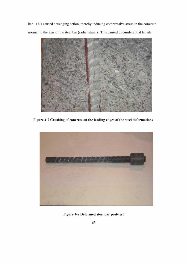
7/28/2019 Weathersby Dis
http://slidepdf.com/reader/full/weathersby-dis 80/280
63
bar. This caused a wedging action, thereby inducing compressive stress in the concrete
normal to the axis of the steel bar (radial strain). This caused circumferential tensile
Figure 4-7 Crushing of concrete on the leading edges of the steel deformations
Figure 4-8 Deformed steel bar post-test
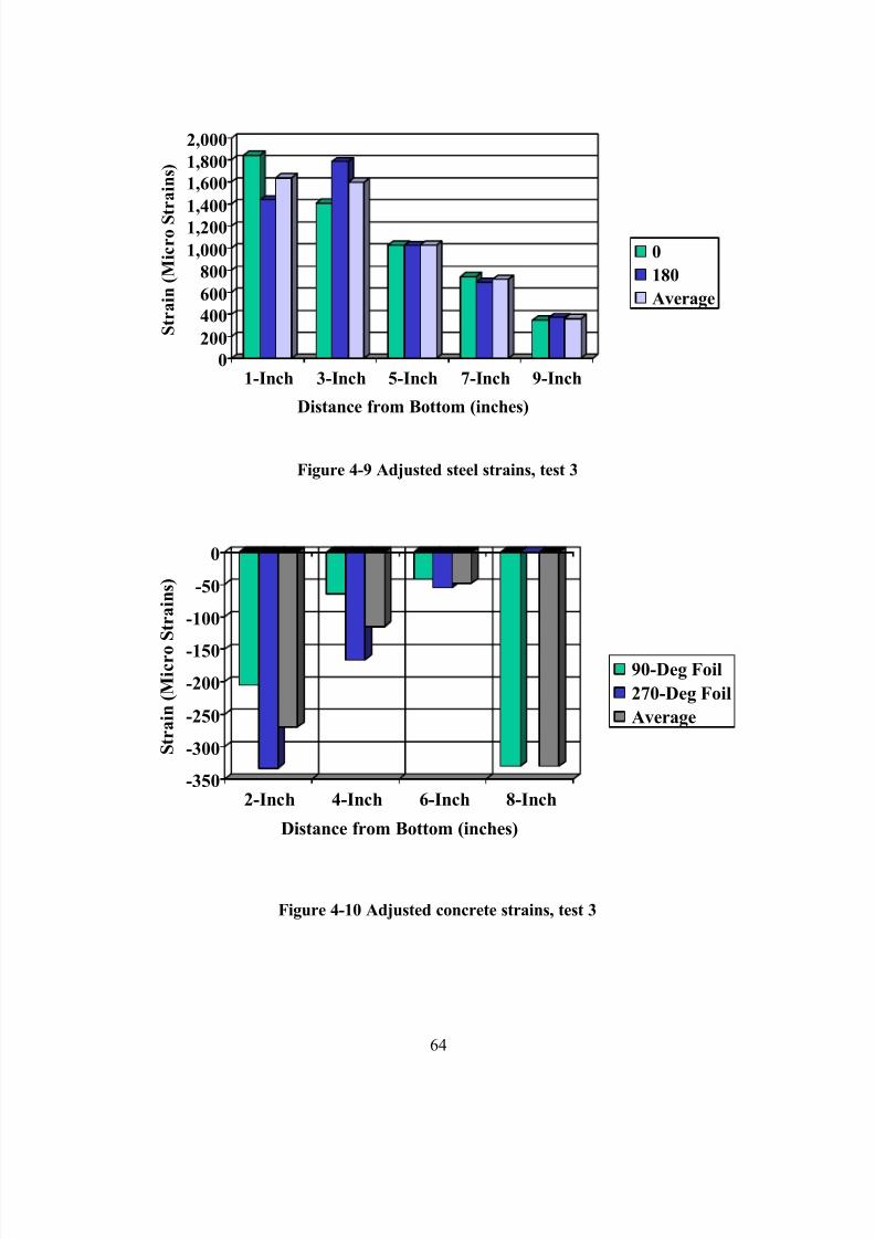
7/28/2019 Weathersby Dis
http://slidepdf.com/reader/full/weathersby-dis 81/280
64
0
200
400
600
800
1,000
1,200
1,400
1,600
1,800
2,000
S t r a i n ( M i c r o S t r a i n s )
1-Inch 3-Inch 5-Inch 7-Inch 9-Inch
Distance from Bottom (inches)
0
180
Average
Figure 4-9 Adjusted steel strains, test 3
-350
-300
-250
-200
-150
-100
-50
0
S t r a i n ( M i c r o
S t r a i n s )
2-Inch 4-Inch 6-Inch 8-Inch
Distance from Bottom (inches)
90-Deg Foil
270-Deg Foil
Average
Figure 4-10 Adjusted concrete strains, test 3
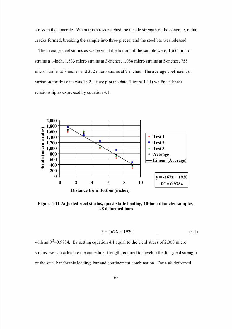
7/28/2019 Weathersby Dis
http://slidepdf.com/reader/full/weathersby-dis 82/280
65
stress in the concrete. When this stress reached the tensile strength of the concrete, radial
cracks formed, breaking the sample into three pieces, and the steel bar was released.
The average steel strains as we begin at the bottom of the sample were, 1,655 micro
strains a 1-inch, 1,533 micro strains at 3-inches, 1,088 micro strains at 5-inches, 758
micro strains at 7-inches and 372 micro strains at 9-inches. The average coefficient of
variation for this data was 18.2. If we plot the data (Figure 4-11) we find a linear
relationship as expressed by equation 4.1:
y = -167x + 1920
R 2
= 0.9784
0200
400
600
800
1,000
1,200
1,400
1,600
1,800
2,000
0 2 4 6 8 10
Distance from Bottom (inches)
S t r a i n ( m i c r o s t r a i n s )
Test 1
Test 2
Test 3
Average
Linear (Average)
Figure 4-11 Adjusted steel strains, quasi-static loading, 10-inch diameter samples,
#8 deformed bars
Y=-167X + 1920 .. (4.1)
with an R 2=0.9784. By setting equation 4.1 equal to the yield stress of 2,000 micro
strains, we can calculate the embedment length required to develop the full yield strength
of the steel bar for this loading, bar and confinement combination. For a #8 deformed
7/28/2019 Weathersby Dis
http://slidepdf.com/reader/full/weathersby-dis 83/280
66
bar, embedded in a 10-inch diameter cylinder loaded quasi-statically, the required
embedment length is 10-1/2-inches.
Since only three of the fiber optic gages returned useful data, it is difficult to make any
definitive statements regarding the comparison of concrete strain measured with the fiber
optic gages vs. that measured with the foil gages, see. However, as shown in Appendix
B, there appears to be no significant variations between the two different types of gages.
The average concrete strains beginning at the bottom were –255.3 micro strains at 2-
inches, -152.7 micro strains at 4-inches, -69.8 micro strains at 6-inches, and –108.8 micro
strains at 8-inches, Figure 4-12. On this set of specimens, and as will be seen on the
remaining tests, there appears to be no relationship between strain and location. In fact,
there is more variation between strains at the same location and test i.e. test 2 CS-01 (-80
micro strains) and CS-02 (-667 micro strains) than there is between the average strains at
different locations i.e. –255.3 micro strains at 2-inches and –69.8 micro strains at 6-
inches. Although there is a very high variation in concrete strain, this is not unusual,
when you consider the non-homogenous nature of concrete, especially on the micro level.
This is caused by not only the variations in strength of the different basic materials, i.e.,
large aggregate vs. small aggregate vs. cement, but also on controllable variations in the
production process, i.e. entrapped air, aggregate separation, moisture evaporation rates,
etc. The average concrete strain was -147 micro strains.
4.2 Impact Loading of a #8 Deformed Bar Embedded in a 10-inch Diameter
Concrete Cylinder
Tests 4, 5 and 6 consisted of a 10 in. diameter cylinder with a number eight deformed
bar subjected to an impact loading. The maximum loads applied to the three specimens
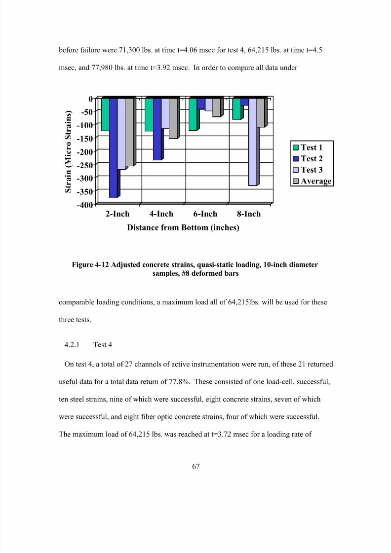
7/28/2019 Weathersby Dis
http://slidepdf.com/reader/full/weathersby-dis 84/280
67
before failure were 71,300 lbs. at time t=4.06 msec for test 4, 64,215 lbs. at time t=4.5
msec, and 77,980 lbs. at time t=3.92 msec. In order to compare all data under
-400-350
-300
-250
-200
-150
-100
-50
0
S t r a i n ( M i c r o S t r a i n s )
2-Inch 4-Inch 6-Inch 8-Inch
Distance from Bottom (inches)
Test 1
Test 2
Test 3
Average
Figure 4-12 Adjusted concrete strains, quasi-static loading, 10-inch diameter
samples, #8 deformed bars
comparable loading conditions, a maximum load all of 64,215lbs. will be used for these
three tests.
4.2.1 Test 4
On test 4, a total of 27 channels of active instrumentation were run, of these 21 returned
useful data for a total data return of 77.8%. These consisted of one load-cell, successful,
ten steel strains, nine of which were successful, eight concrete strains, seven of which
were successful, and eight fiber optic concrete strains, four of which were successful.
The maximum load of 64,215 lbs. was reached at t=3.72 msec for a loading rate of
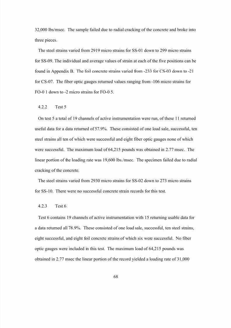
7/28/2019 Weathersby Dis
http://slidepdf.com/reader/full/weathersby-dis 85/280
68
32,000 lbs/msec. The sample failed due to radial cracking of the concrete and broke into
three pieces.
The steel strains varied from 2919 micro strains for SS-01 down to 299 micro strains
for SS-09. The individual and average values of strain at each of the five positions can be
found in Appendix B. The foil concrete strains varied from -233 for CS-03 down to -21
for CS-07. The fiber optic gauges returned values ranging from -106 micro strains for
FO-0 1 down to -2 micro strains for FO-0 5.
4.2.2 Test 5
On test 5 a total of 19 channels of active instrumentation were run, of these 11 returned
useful data for a data returned of 57.9%. These consisted of one load sale, successful, ten
steel strains all ten of which were successful and eight fiber optic gauges none of which
were successful. The maximum load of 64,215 pounds was obtained in 2.77 msec. The
linear portion of the loading rate was 19,600 lbs./msec. The specimen failed due to radial
cracking of the concrete.
The steel strains varied from 2930 micro strains for SS-02 down to 273 micro strains
for SS-10. There were no successful concrete strain records for this test.
4.2.3 Test 6
Test 6 contains 19 channels of active instrumentation with 15 returning usable data for
a data returned all 78.9%. These consisted of one load sale, successful, ten steel strains,
eight successful, and eight foil concrete strains of which six were successful. No fiber
optic gauges were included in this test. The maximum load of 64,215 pounds was
obtained in 2.77 msec the linear portion of the record yielded a loading rate of 31,000
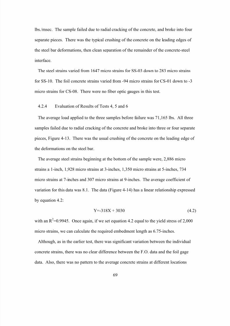
7/28/2019 Weathersby Dis
http://slidepdf.com/reader/full/weathersby-dis 86/280
69
lbs./msec. The sample failed due to radial cracking of the concrete, and broke into four
separate pieces. There was the typical crushing of the concrete on the leading edges of
the steel bar deformations, then clean separation of the remainder of the concrete-steel
interface.
The steel strains varied from 1647 micro strains for SS-03 down to 283 micro strains
for SS-10. The foil concrete strains varied from -94 micro strains for CS-01 down to -3
micro strains for CS-08. There were no fiber optic gauges in this test.
4.2.4 Evaluation of Results of Tests 4, 5 and 6
The average load applied to the three samples before failure was 71,165 lbs. All three
samples failed due to radial cracking of the concrete and broke into three or four separate
pieces, Figure 4-13. There was the usual crushing of the concrete on the leading edge of
the deformations on the steel bar.
The average steel strains beginning at the bottom of the sample were, 2,886 micro
strains a 1-inch, 1,928 micro strains at 3-inches, 1,350 micro strains at 5-inches, 734
micro strains at 7-inches and 307 micro strains at 9-inches. The average coefficient of
variation for this data was 8.1. The data (Figure 4-14) has a linear relationship expressed
by equation 4.2:
Y=-318X + 3030 (4.2)
with an R 2=0.9945. Once again, if we set equation 4.2 equal to the yield stress of 2,000
micro strains, we can calculate the required embedment length as 6.75-inches.
Although, as in the earlier test, there was significant variation between the individual
concrete strains, there was no clear difference between the F.O. data and the foil gage
data. Also, there was no pattern to the average concrete strains at different locations
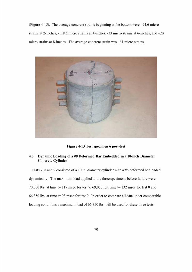
7/28/2019 Weathersby Dis
http://slidepdf.com/reader/full/weathersby-dis 87/280
70
(Figure 4-15). The average concrete strains beginning at the bottom were –94.6 micro
strains at 2-inches, -118.6 micro strains at 4-inches, -33 micro strains at 6-inches, and –20
micro strains at 8-inches. The average concrete strain was –61 micro strains.
Figure 4-13 Test specimen 6 post-test
4.3 Dynamic Loading of a #8 Deformed Bar Embedded in a 10-inch Diameter
Concrete Cylinder
Tests 7, 8 and 9 consisted of a 10 in. diameter cylinder with a #8 deformed bar loaded
dynamically. The maximum load applied to the three specimens before failure were
70,300 lbs. at time t= 117 msec for test 7, 69,050 lbs. time t= 132 msec for test 8 and
66,350 lbs. at time t= 93 msec for test 9. In order to compare all data under comparable
loading conditions a maximum load of 66,350 lbs. will be used for these three tests.
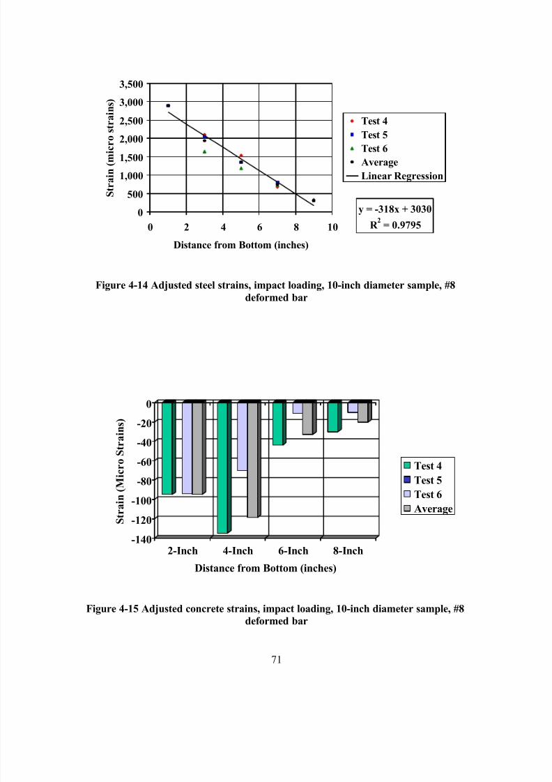
7/28/2019 Weathersby Dis
http://slidepdf.com/reader/full/weathersby-dis 88/280
71
y = -318x + 3030
R 2
= 0.9795
0
500
1,000
1,500
2,000
2,500
3,000
3,500
0 2 4 6 8 10
Distance from Bottom (inches)
S t r a i n ( m i c r o
s t r a i n s )
Test 4
Test 5Test 6
Average
Linear Regression
Figure 4-14 Adjusted steel strains, impact loading, 10-inch diameter sample, #8
deformed bar
-140
-120
-100
-80
-60
-40
-20
0
S t r a i n ( M i c r o S t r a i n s )
2-Inch 4-Inch 6-Inch 8-Inch
Distance from Bottom (inches)
Test 4
Test 5
Test 6
Average
Figure 4-15 Adjusted concrete strains, impact loading, 10-inch diameter sample, #8
deformed bar
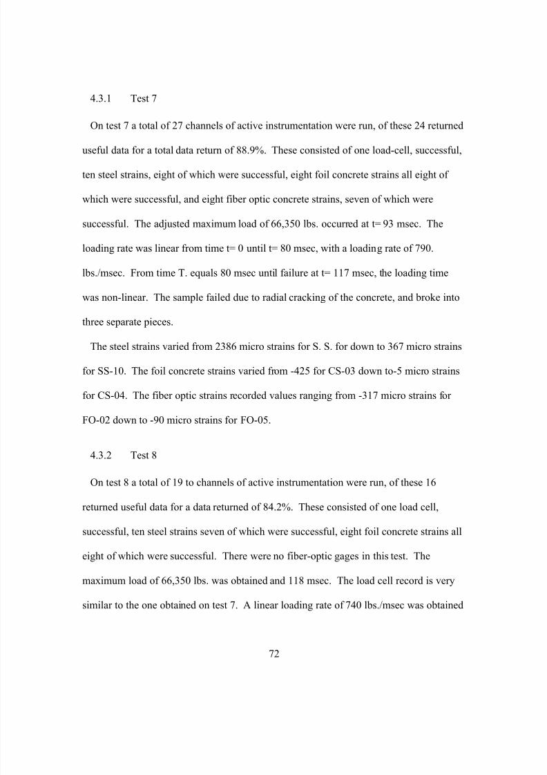
7/28/2019 Weathersby Dis
http://slidepdf.com/reader/full/weathersby-dis 89/280
72
4.3.1 Test 7
On test 7 a total of 27 channels of active instrumentation were run, of these 24 returned
useful data for a total data return of 88.9%. These consisted of one load-cell, successful,
ten steel strains, eight of which were successful, eight foil concrete strains all eight of
which were successful, and eight fiber optic concrete strains, seven of which were
successful. The adjusted maximum load of 66,350 lbs. occurred at t= 93 msec. The
loading rate was linear from time t= 0 until t= 80 msec, with a loading rate of 790.
lbs./msec. From time T. equals 80 msec until failure at t= 117 msec, the loading time
was non-linear. The sample failed due to radial cracking of the concrete, and broke into
three separate pieces.
The steel strains varied from 2386 micro strains for S. S. for down to 367 micro strains
for SS-10. The foil concrete strains varied from -425 for CS-03 down to-5 micro strains
for CS-04. The fiber optic strains recorded values ranging from -317 micro strains for
FO-02 down to -90 micro strains for FO-05.
4.3.2 Test 8
On test 8 a total of 19 to channels of active instrumentation were run, of these 16
returned useful data for a data returned of 84.2%. These consisted of one load cell,
successful, ten steel strains seven of which were successful, eight foil concrete strains all
eight of which were successful. There were no fiber-optic gages in this test. The
maximum load of 66,350 lbs. was obtained and 118 msec. The load cell record is very
similar to the one obtained on test 7. A linear loading rate of 740 lbs./msec was obtained
7/28/2019 Weathersby Dis
http://slidepdf.com/reader/full/weathersby-dis 90/280
73
from t= 0 msec until t= 80 msec. The loading rate was nonlinear from t= 80 msec until
failure at t= 132 msec. The sample failed due to radial cracking and broke into 3 pieces.
The steel strains varied from a high value of 2763 micro strains for SS-04 to a low
value of 386 micro strains for SS-10. The foil concrete strains varied from -167 micro
strains for CS-02 down to-6 micro strains for CS-07.
4.3.3 Test 9
On test nine a total of 19 channels of active instrumentation were run, of these 16
returned useful data for a data return of 84.2%. These consisted of one load cell,
successful, ten concrete strains seven of which were successful, and eight foil concrete
strains all eight of which were successful. The maximum load of 66,350 lbs. was
obtained in 92 msec. The loading rate of 825 lbs./msec remain linear until t= 80 msec.
The sample failed due to radial cracking and broke into 3 pieces. The loading rate was
then nonlinear until failure at t= 92 msec.
The steel strains varied from 2280 micro strains for SS-03 down to 545 micro strains
for SS-10. The foil concrete strains varied from a high value of -669 micro strains for
CS-04 to less than one micro strain for CS-07.
4.3.4 Evaluation of Results of Tests 7, 8 and 9
The average load applied to the three samples before failure was 68,566 lbs. All three
samples failed due to radial cracking of the concrete and broke into three separate pieces,
Figure 4-16. There was crushing of the concrete on the leading edge of the deformations
on the steel bar.
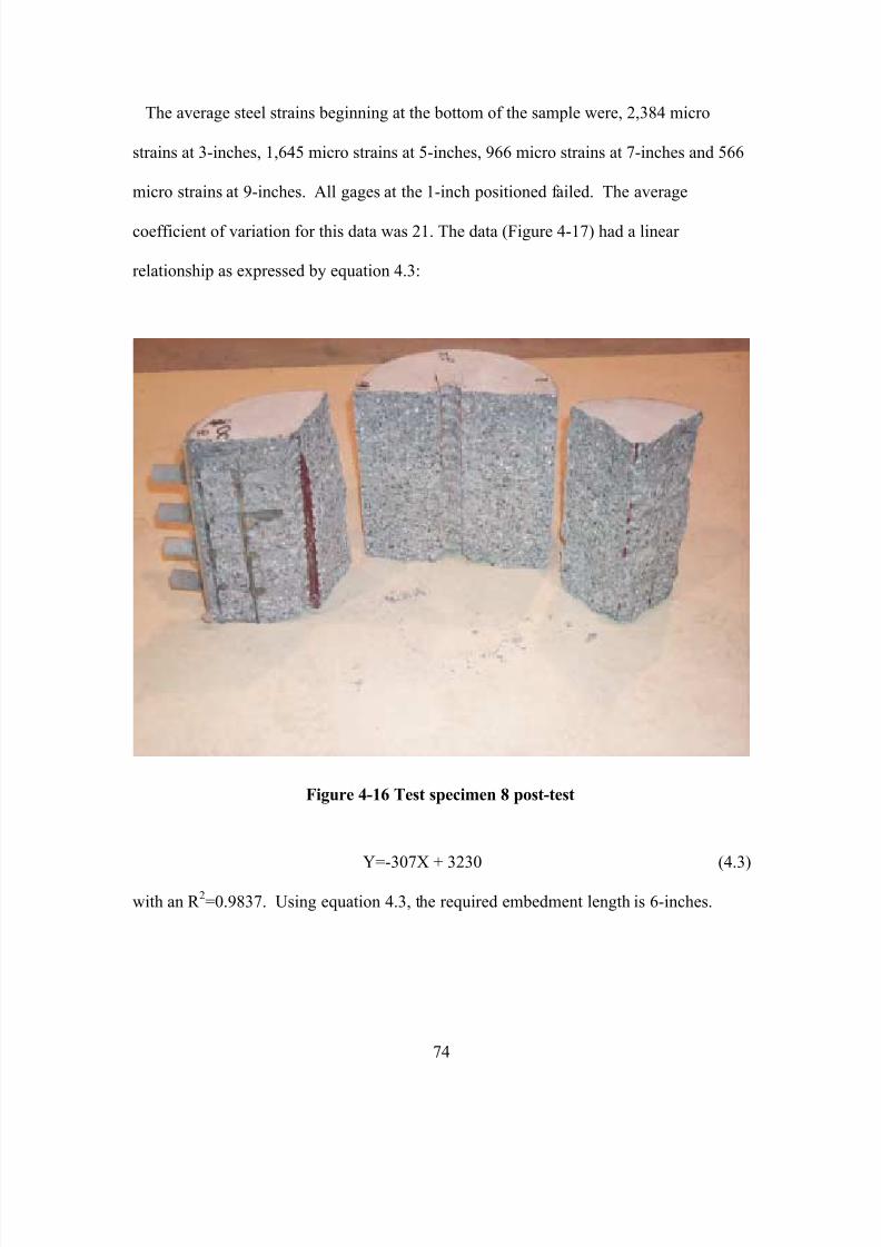
7/28/2019 Weathersby Dis
http://slidepdf.com/reader/full/weathersby-dis 91/280
74
The average steel strains beginning at the bottom of the sample were, 2,384 micro
strains at 3-inches, 1,645 micro strains at 5-inches, 966 micro strains at 7-inches and 566
micro strains at 9-inches. All gages at the 1-inch positioned failed. The average
coefficient of variation for this data was 21. The data (Figure 4-17) had a linear
relationship as expressed by equation 4.3:
Figure 4-16 Test specimen 8 post-test
Y=-307X + 3230 (4.3)
with an R 2=0.9837. Using equation 4.3, the required embedment length is 6-inches.
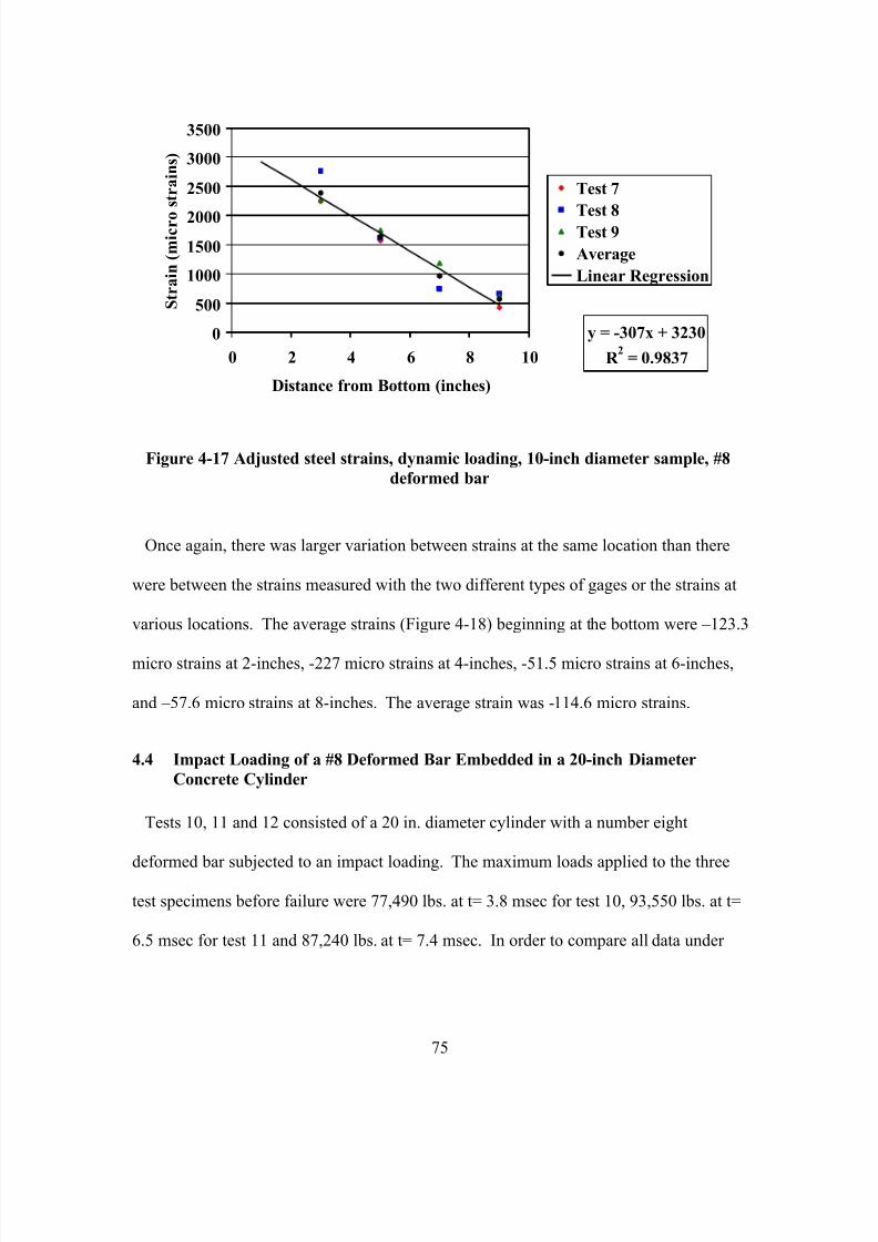
7/28/2019 Weathersby Dis
http://slidepdf.com/reader/full/weathersby-dis 92/280
75
y = -307x + 3230
R 2
= 0.9837
0
500
1000
1500
2000
2500
3000
3500
0 2 4 6 8 10
Distance from Bottom (inches)
S t r a i n ( m i c r o
s t r a i n s )
Test 7
Test 8Test 9
Average
Linear Regression
Figure 4-17 Adjusted steel strains, dynamic loading, 10-inch diameter sample, #8
deformed bar
Once again, there was larger variation between strains at the same location than there
were between the strains measured with the two different types of gages or the strains at
various locations. The average strains (Figure 4-18) beginning at the bottom were –123.3
micro strains at 2-inches, -227 micro strains at 4-inches, -51.5 micro strains at 6-inches,
and –57.6 micro strains at 8-inches. The average strain was -114.6 micro strains.
4.4 Impact Loading of a #8 Deformed Bar Embedded in a 20-inch Diameter
Concrete Cylinder
Tests 10, 11 and 12 consisted of a 20 in. diameter cylinder with a number eight
deformed bar subjected to an impact loading. The maximum loads applied to the three
test specimens before failure were 77,490 lbs. at t= 3.8 msec for test 10, 93,550 lbs. at t=
6.5 msec for test 11 and 87,240 lbs. at t= 7.4 msec. In order to compare all data under
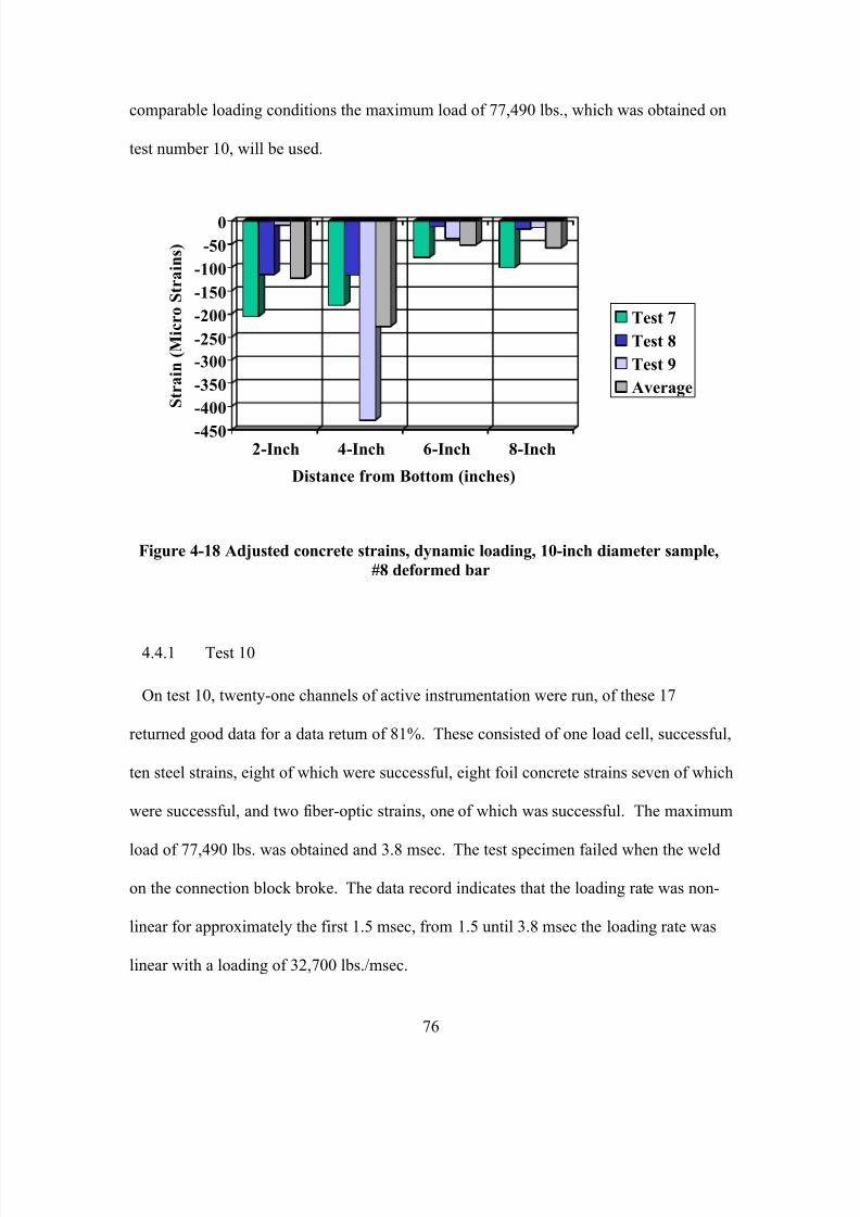
7/28/2019 Weathersby Dis
http://slidepdf.com/reader/full/weathersby-dis 93/280
76
comparable loading conditions the maximum load of 77,490 lbs., which was obtained on
test number 10, will be used.
-450
-400
-350
-300
-250
-200
-150
-100
-50
0
S t r a i n ( M i c r o S t r a i n s )
2-Inch 4-Inch 6-Inch 8-Inch
Distance from Bottom (inches)
Test 7
Test 8
Test 9
Average
Figure 4-18 Adjusted concrete strains, dynamic loading, 10-inch diameter sample,
#8 deformed bar
4.4.1 Test 10
On test 10, twenty-one channels of active instrumentation were run, of these 17
returned good data for a data return of 81%. These consisted of one load cell, successful,
ten steel strains, eight of which were successful, eight foil concrete strains seven of which
were successful, and two fiber-optic strains, one of which was successful. The maximum
load of 77,490 lbs. was obtained and 3.8 msec. The test specimen failed when the weld
on the connection block broke. The data record indicates that the loading rate was non-
linear for approximately the first 1.5 msec, from 1.5 until 3.8 msec the loading rate was
linear with a loading of 32,700 lbs./msec.
7/28/2019 Weathersby Dis
http://slidepdf.com/reader/full/weathersby-dis 94/280
77
The steel strains varied from a maximum of 2390 micro strains for SS-04 down to a minimum
of 390 micro strains for SS-10. The foil concrete strains varied from a maximum of -435 micro
strains for CS-05 down to a minimum of -82 micro strains for CS-01. The one successful fiber-
optic record was FO-01, which returned a peak value of -138 micro strains.
4.4.2 Test 11
On test 11, 27 channels of active instrumentation were run with 17 returning good data
for a data return of 63%. This consisted of one load cell, which was successful, ten steel
strains two of which were successful, eight foil concrete strains all eight of which were
successful, and eight fiber-optic gages, six of which were successful. The adjusted
maximum load of 77,490 lbs. was obtained in 4.79 msec. The data record shows the
customary two msec nonlinear beginning followed by a linear loading of 33,400
lbs./msec until t= 3.3 msec. There is then a change in slope to 8,600 lbs./msec until
ultimate failure at t= 6.49 msec. The sample failed due to yielding of the weld joints on
the connection block.
The maximum steel strains recorded on this test was 754 micro strains for SS-09 and
the minimum was 487 micro strains for SS-10 the concrete foil gages recorded a
maximum strain of -479 micro strains for CS-01 to a minimum of -16 micro strains for
CS-04. The fiber-optic strains varied from a maximum of -429 micro strains for FO-07
to a minimum of -85 micro strains for FO-01.
4.4.3 Test 12
On test 12, a total of twenty-seven channels of active instrumentation were run with 20
channels returning usable data. This gave a data return of 74.1%. These consisted of one
load cell, which was successful, ten steel strains, five of which were successful, eight foil
7/28/2019 Weathersby Dis
http://slidepdf.com/reader/full/weathersby-dis 95/280
78
concrete strains, seven of which were successful and eight fiber-optic strains, seven of
which were also successful. The adjusted maximum load of 77,490 lbs. was obtained in
5.4 msec. The loading rate was nonlinear on both ends with a linear loading rate of
33,300 lbs./msec between t= 2 msec and t= 4 msec. The load then drops drastically to
around 12 msec, at which time it begins to rebounds back to around 90,000 lbs. This
second loading is not real but most likely caused by the loader abruptly reaching the
limits of its stroke. The sample had an identical failure to the samples in test 10 and 11.
The maximum steel strain recorded was 1790 micro strains for SS-06 and the minimum
was 282 micro strains for SS-09. The foil concrete strains varied from a maximum of -
517 micro strains for CS-01 down to a minimum of -20 micro strains for CS-05 the fiber
optic strains varied from a maximum of -267 micro strains for FO-03 to a minimum of -
13.6 micro strains for FO-02.
4.4.4 Evaluation of Results of Tests 10, 11 and 12
The average load applied to the three samples before failure was 86,100 lbs. All three
samples failed due to failure of the welds between the connecting block and the #8
reinforcing bar, Figure 4-19.
The average steel strains beginning at the bottom of the sample were, 2,345 micro
strains at 3-inches, 1,655 micro strains at 5-inches, 1020 micro strains at 7-inches and
478 micro strains at 9-inches. All gages at the 1-inch positioned failed. The average
coefficient of variation for this data was 22. The data (Figure 4-20) had a linear
relationship as expressed by equation 4.4:
Y=-312X + 3250 (4.4)
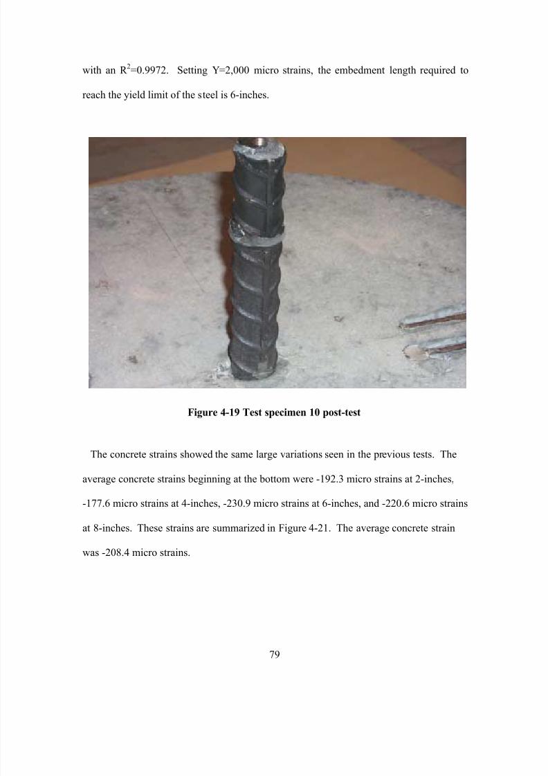
7/28/2019 Weathersby Dis
http://slidepdf.com/reader/full/weathersby-dis 96/280
79
with an R 2=0.9972. Setting Y=2,000 micro strains, the embedment length required to
reach the yield limit of the steel is 6-inches.
Figure 4-19 Test specimen 10 post-test
The concrete strains showed the same large variations seen in the previous tests. The
average concrete strains beginning at the bottom were -192.3 micro strains at 2-inches,
-177.6 micro strains at 4-inches, -230.9 micro strains at 6-inches, and -220.6 micro strains
at 8-inches. These strains are summarized in Figure 4-21. The average concrete strain
was -208.4 micro strains.
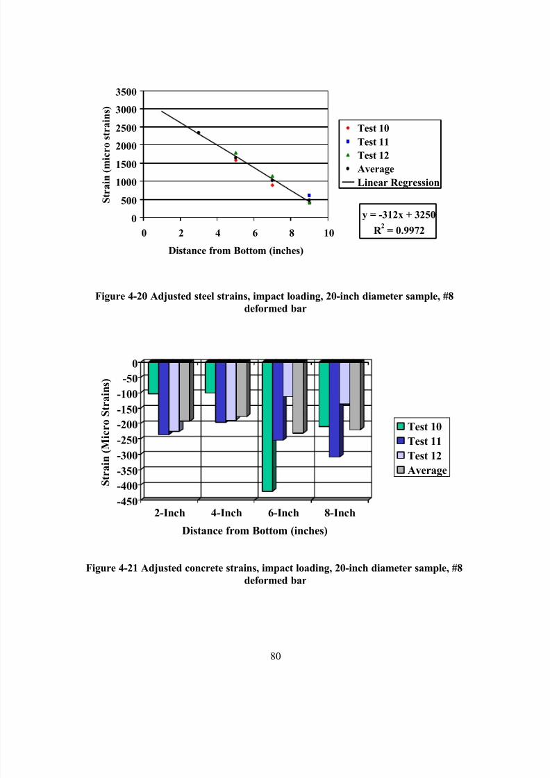
7/28/2019 Weathersby Dis
http://slidepdf.com/reader/full/weathersby-dis 97/280
80
y = -312x + 3250
R 2
= 0.99720
500
1000
1500
2000
2500
3000
3500
0 2 4 6 8 10
Distance from Bottom (inches)
S t r a i n ( m i c r o s t r a i n s )
Test 10
Test 11
Test 12
Average
Linear Regression
Figure 4-20 Adjusted steel strains, impact loading, 20-inch diameter sample, #8
deformed bar
-450
-400
-350
-300
-250
-200-150
-100
-50
0
S t r a i n ( M i c r o S t r a i n s )
2-Inch 4-Inch 6-Inch 8-Inch
Distance from Bottom (inches)
Test 10
Test 11
Test 12
Average
Figure 4-21 Adjusted concrete strains, impact loading, 20-inch diameter sample, #8
deformed bar
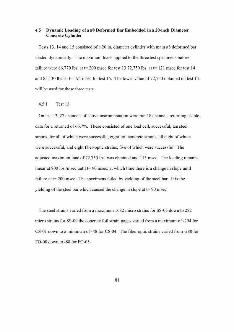
7/28/2019 Weathersby Dis
http://slidepdf.com/reader/full/weathersby-dis 98/280
81
4.5 Dynamic Loading of a #8 Deformed Bar Embedded in a 20-inch Diameter
Concrete Cylinder
Tests 13, 14 and 15 consisted of a 20 in. diameter cylinder with main #8 deformed bar
loaded dynamically. The maximum loads applied to the three test specimens before
failure were 86,770 lbs. at t= 200 msec for test 13 72,750 lbs. at t= 121 msec for test 14
and 85,130 lbs. at t= 194 msec for test 15. The lower value of 72,750 obtained on test 14
will be used for these three tests.
4.5.1 Test 13
On test 13, 27 channels of active instrumentation were run 18 channels returning usable
data for a returned of 66.7%. These consisted of one load cell, successful, ten steel
strains, for all of which were successful, eight foil concrete strains, all eight of which
were successful, and eight fiber-optic strains, five of which were successful. The
adjusted maximum load of 72,750 lbs. was obtained and 115 msec. The loading remains
linear at 800 lbs./msec until t= 90 msec, at which time there is a change in slope until
failure at t= 200 msec. The specimens failed by yielding of the steel bar. It is the
yielding of the steel bar which caused the change in slope at t= 90 msec.
The steel strains varied from a maximum 1682 micro strains for SS-05 down to 282
micro strains for SS-09 the concrete foil strain gages varied from a maximum of -294 for
CS-01 down to a minimum of -48 for CS-04. The fiber optic strains varied from -280 for
FO-08 down to -88 for FO-05.
7/28/2019 Weathersby Dis
http://slidepdf.com/reader/full/weathersby-dis 99/280
82
4.5.2 Test 14
On test 14, 27 channels were run with 20 returning good data for a total return 74.1%.
These consisted of one load cell, ten concrete strains, five of which were successful, eight
foil concrete strains, all eight of which were successful, and eight fiber optic strains, six
of which were successful. The maximum load of 72,750 lbs. was obtained in 121 msec.
The loading rate remained linear at 780 lbs./msec until t= 85 msec, at which time there is
a change in slope until failure at 121 msec. The sample failed due to yielding of the steel
bar, it is this yielding which caused the change in slope.
The steel strains varied from 2690 micro strains for SS-04 down to 420 micro strains
for SS-10. The foil concrete strains varied from a maximum of -331 micro strains for
CS-06 down to five micro strains for CS-07. The fiber optic strains varied from -328
mica strains for FO-05 down to -158 micro strains for FO-06.
4.5.3 Test 15
On test 15, 27 channels of instrumentation were run 22 returned usable data for a
returned of 81.5%. These consisted of one load cell, ten steel strains, eight of which were
successful, eight concrete strains, seven of which were successful, and eight fiber optics
strain gages, six of which were successful. The adjusted maximum load of 72,750 lbs.
was obtained in 126 msec. The load cell data plot shows the customary linear loading
rate of 780 lbs./msec until t= 90 msec and then the reduction in slope until the failure at
t= 194 msec. Once again this change in slope is due to the yielding of the steel bar.
The steel strains varied from a maximum of 3600 into micro strains for SS-03 down to
270 mica strains for SS-09. The foil concrete strains varied from a maximum of -279
7/28/2019 Weathersby Dis
http://slidepdf.com/reader/full/weathersby-dis 100/280
83
more strains for CS-05 to -29 micro strains for CS-04 the fiber optic readings varied from
a maximum of -384 micro strains for FO-01 to -87 micro strains for FO-04.
4.5.4 Evaluation of Results of Tests 13, 14 and 15
The average load applied to the three samples before failure was 81,550 lbs. Samples
13 and 14 failed due to yielding of the steel bar above the connection block as shown in
Figure 4-22. Sample 15 failed due to the welds on the connection block breaking.
The average steel strains beginning at the bottom of the sample were, 3,074 micro strains at 3-
inches, 1,798 micro strains at 5-inches, 1066 micro strains at 7-inches and 434 micro strains at 9-
inches. All gages at the 1-inch positioned failed. The average coefficient of variation for this
data was 15.3. The data (Figure 4-23) had a linear relationship as expressed by equation 4.5:
Y=-433X + 4190 (4.5)
with an R 2=0.9706. Setting Y=2,000 micro strains, we calculate the embedment length
required to reach the yield strength of the steel as 5-inches.
The average concrete strains beginning at the bottom were -184.6 micro strains at 2-
inches, -162.7 micro strains at 4-inches, -176.7 micro strains at 6-inches, and -167.4
micro strains at 8-inches (Figure 4-24). The average concrete strain was -171.9 micro
strains.
4.6 Quasi-Static Loading of a #8 Deformed Bar Embedded in a 20-inch Diameter
Concrete Cylinder
Test 16, 17 and 18 consisted of a 20 in. diameter cylinder with a number eight
deformed bar loaded statically. The maximum loads applied to the three test specimens
before failure were 71,770 lbs. at t= 578 seconds for test 16, 60,600 lbs. at t= 288
seconds, for test 17, and 63,480 lbs. at t= 337 sec., for test 18. In order to compare all
7/28/2019 Weathersby Dis
http://slidepdf.com/reader/full/weathersby-dis 101/280
84
data under comparable loading conditions a maximum load of 60,600 lbs. will be used for
these three tests.
Figure 4-22 Test specimen 13 post-test
y = -433x + 4190
R 2
= 0.9706
0
500
1000
1500
2000
2500
3000
3500
4000
0 2 4 6 8 10
Distance from Bottom (inches)
S t r a i n ( m i c r o s t r a i n s )
Test 13
Test 14
Test 15
Average
Linear Regression
Figure 4-23 Adjusted steel strains, dynamic loading, 20-inch diameter sample, #8
deformed bar
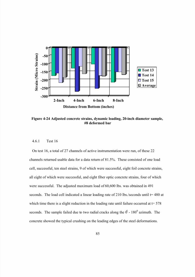
7/28/2019 Weathersby Dis
http://slidepdf.com/reader/full/weathersby-dis 102/280
85
-300
-250
-200
-150
-100
-50
0
S t r a i n ( M i c r o S t r a i n s )
2-Inch 4-Inch 6-Inch 8-Inch
Distance from Bottom (inches)
Test 13
Test 14
Test 15
Average
Figure 4-24 Adjusted concrete strains, dynamic loading, 20-inch diameter sample,
#8 deformed bar
4.6.1 Test 16
On test 16, a total of 27 channels of active instrumentation were run, of these 22
channels returned usable data for a data return of 81.5%. These consisted of one load
cell, successful, ten steel strains, 9 of which were successful, eight foil concrete strains,
all eight of which were successful, and eight fiber optic concrete strains, four of which
were successful. The adjusted maximum load of 60,600 lbs. was obtained in 491
seconds. The load cell indicated a linear loading rate of 210 lbs./seconds until t= 480 at
which time there is a slight reduction in the loading rate until failure occurred at t= 578
seconds. The sample failed due to two radial cracks along the 00
- 1800
azimuth. The
concrete showed the typical crushing on the leading edges of the steel deformations.
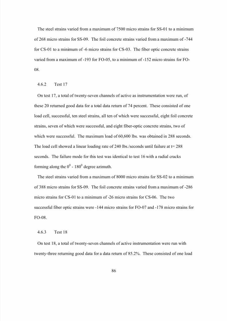
7/28/2019 Weathersby Dis
http://slidepdf.com/reader/full/weathersby-dis 103/280
86
The steel strains varied from a maximum of 7500 micro strains for SS-01 to a minimum
of 268 micro strains for SS-09. The foil concrete strains varied from a maximum of -744
for CS-01 to a minimum of -6 micro strains for CS-03. The fiber optic concrete strains
varied from a maximum of -193 for FO-05, to a minimum of -152 micro strains for FO-
08.
4.6.2 Test 17
On test 17, a total of twenty-seven channels of active as instrumentation were run, of
these 20 returned good data for a total data return of 74 percent. These consisted of one
load cell, successful, ten steel strains, all ten of which were successful, eight foil concrete
strains, seven of which were successful, and eight fiber-optic concrete strains, two of
which were successful. The maximum load of 60,600 lbs. was obtained in 288 seconds.
The load cell showed a linear loading rate of 240 lbs./seconds until failure at t= 288
seconds. The failure mode for this test was identical to test 16 with a radial cracks
forming along the 0
0
- 180
0
degree azimuth.
The steel strains varied from a maximum of 8000 micro strains for SS-02 to a minimum
of 388 micro strains for SS-09. The foil concrete strains varied from a maximum of -286
micro strains for CS-01 to a minimum of -26 micro strains for CS-06. The two
successful fiber optic strains were -144 micro strains for FO-07 and -178 micro strains for
FO-08.
4.6.3 Test 18
On test 18, a total of twenty-seven channels of active instrumentation were run with
twenty-three returning good data for a data return of 85.2%. These consisted of one load
7/28/2019 Weathersby Dis
http://slidepdf.com/reader/full/weathersby-dis 104/280
87
cell, successful, ten steel strains, all ten of which were successful, eight foil concrete
strains, seven of which were successful, and eight fiber optic concrete strains, five of
which were successful. The adjusted maximum load of 60,600 lbs. was obtained in 321
seconds. The load cell showed a linear loading rate of 240 lbs./seconds until t= 320
seconds at which time there is a reduction in loading rate until failure at t= 337 seconds.
The sample failed due to radial cracking along the 00
- 1800
azimuth.
The steel strains varied from a maximum of 13,340 micro strains for SS-02, to a
minimum of 275 micro strains for SS-10. The foil concrete strains varied from a
maximum of -515 micro strains for CS-03 to a minimum of -59 micro strains for CS-06.
The fiber optic concrete strains varied from a -203 for FO-06 down to -115 micro strains
for FO-04.
4.6.4 Evaluation of Results of Tests 16, 17 and 18
The average load applied to the three samples before failure was 65,300 lbs. All three
samples failed due to radial cracking of the concrete and broke into two separate pieces,
with the crack forming along the 00
– 1800
azimuth, Figure 4-25. There was crushing of
the concrete on the leading edge of the deformations on the steel bar.
The average steel strains beginning at the bottom of the sample were, 9,022 micro
strains at 1-inch, 1866 micro strains at 3-inches, 1,327 micro strains at 5-inches, 866
micro strains at 7-inches and 356 micro strains at 9-inches. If we disregard the strain data
from the 1-inch position, which was clearly in the plastic range, we get an average
coefficient of variation for this data of 12 and a linear relationship (Figure 4-26)
expressed by equation 4.6:
Y=-250X + 2600 (4.6)
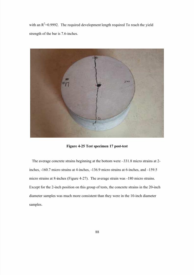
7/28/2019 Weathersby Dis
http://slidepdf.com/reader/full/weathersby-dis 105/280
88
with an R 2=0.9992. The required development length required To reach the yield
strength of the bar is 7.6-inches.
Figure 4-25 Test specimen 17 post-test
The average concrete strains beginning at the bottom were –331.8 micro strains at 2-
inches, -160.7 micro strains at 4-inches, -136.9 micro strains at 6-inches, and –159.5
micro strains at 8-inches (Figure 4-27). The average strain was -180 micro strains.
Except for the 2-inch position on this group of tests, the concrete strains in the 20-inch
diameter samples was much more consistent than they were in the 10-inch diameter
samples.
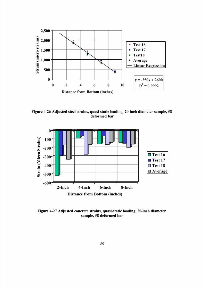
7/28/2019 Weathersby Dis
http://slidepdf.com/reader/full/weathersby-dis 106/280
89
y = -250x + 2600
R 2
= 0.9992
0
500
1,000
1,500
2,000
2,500
0 2 4 6 8 10
Distance from Bottom (inches)
S t r a i n ( m i c r o
s t r a i n s )
Test 16
Test 17Test18
Average
Linear Regression
Figure 4-26 Adjusted steel strains, quasi-static loading, 20-inch diameter sample, #8
deformed bar
-600
-500
-400
-300
-200
-100
0
S t r a i n ( M i c r o
S t r a i n s )
2-Inch 4-Inch 6-Inch 8-Inch
Distance from Bottom (inches)
Test 16
Test 17
Test 18
Average
Figure 4-27 Adjusted concrete strains, quasi-static loading, 20-inch diameter
sample, #8 deformed bar
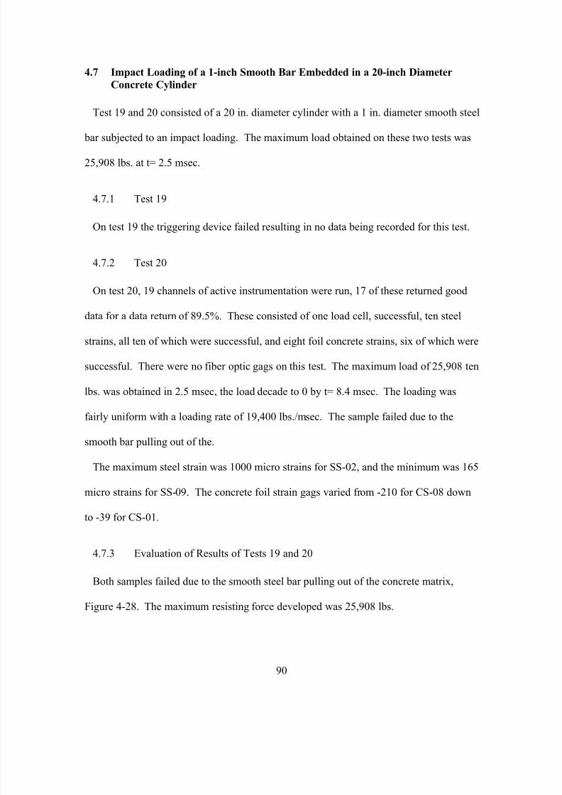
7/28/2019 Weathersby Dis
http://slidepdf.com/reader/full/weathersby-dis 107/280
90
4.7 Impact Loading of a 1-inch Smooth Bar Embedded in a 20-inch Diameter
Concrete Cylinder
Test 19 and 20 consisted of a 20 in. diameter cylinder with a 1 in. diameter smooth steel
bar subjected to an impact loading. The maximum load obtained on these two tests was
25,908 lbs. at t= 2.5 msec.
4.7.1 Test 19
On test 19 the triggering device failed resulting in no data being recorded for this test.
4.7.2 Test 20
On test 20, 19 channels of active instrumentation were run, 17 of these returned good
data for a data return of 89.5%. These consisted of one load cell, successful, ten steel
strains, all ten of which were successful, and eight foil concrete strains, six of which were
successful. There were no fiber optic gags on this test. The maximum load of 25,908 ten
lbs. was obtained in 2.5 msec, the load decade to 0 by t= 8.4 msec. The loading was
fairly uniform with a loading rate of 19,400 lbs./msec. The sample failed due to the
smooth bar pulling out of the.
The maximum steel strain was 1000 micro strains for SS-02, and the minimum was 165
micro strains for SS-09. The concrete foil strain gags varied from -210 for CS-08 down
to -39 for CS-01.
4.7.3 Evaluation of Results of Tests 19 and 20
Both samples failed due to the smooth steel bar pulling out of the concrete matrix,
Figure 4-28. The maximum resisting force developed was 25,908 lbs.
7/28/2019 Weathersby Dis
http://slidepdf.com/reader/full/weathersby-dis 108/280
91
Figure 4-28 Test specimen 20 post-test
The average steel strains beginning at the bottom of the sample were, 885 micro strains
at 1-inch, 731 micro strains at 3-inches, 570 micro strains at 5-inches, 356 micro strains
at 7-inches and 173 micro strains at 9-inches. Due to the limited number of data points,
no reference can be made to the coefficient of variation, however, the available data does
show a linear relationship (Figure 4-29) expressed by equation 4.7
Y=-90X + 993 (4.7)
with an R 2=0.9961. For the smooth bar to be able to develop its full yield strength, an
embedment length of 21-inches would be required.
There is very little data on the concrete strains for this set up since only two tests were
planned, and one of those failed. Therefore there are only six concrete strain readings
available. These tend to indicate a linear relationship to the data with the average strain
beginning at the bottom being –39 micro strains at 2-inches, -90 micro strains at 4-inches,
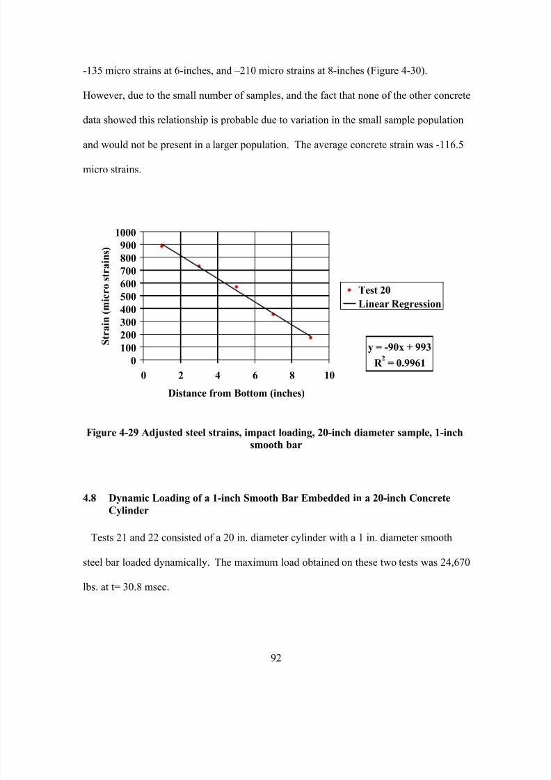
7/28/2019 Weathersby Dis
http://slidepdf.com/reader/full/weathersby-dis 109/280
92
-135 micro strains at 6-inches, and –210 micro strains at 8-inches (Figure 4-30).
However, due to the small number of samples, and the fact that none of the other concrete
data showed this relationship is probable due to variation in the small sample population
and would not be present in a larger population. The average concrete strain was -116.5
micro strains.
y = -90x + 993
R 2
= 0.99610
100
200
300
400
500
600700
800
900
1000
0 2 4 6 8 10
Distance from Bottom (inches)
S t r a i n ( m i c r o s t r
a i n s )
Test 20
Linear Regression
Figure 4-29 Adjusted steel strains, impact loading, 20-inch diameter sample, 1-inch
smooth bar
4.8 Dynamic Loading of a 1-inch Smooth Bar Embedded in a 20-inch Concrete
Cylinder
Tests 21 and 22 consisted of a 20 in. diameter cylinder with a 1 in. diameter smooth
steel bar loaded dynamically. The maximum load obtained on these two tests was 24,670
lbs. at t= 30.8 msec.
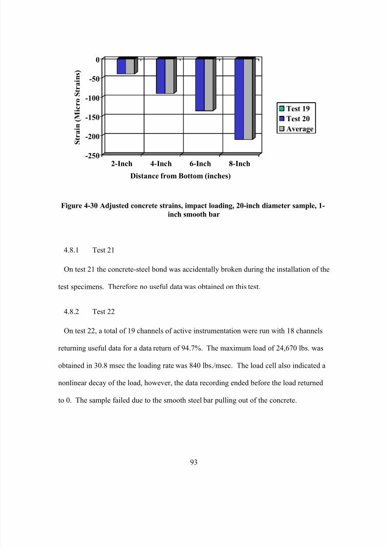
7/28/2019 Weathersby Dis
http://slidepdf.com/reader/full/weathersby-dis 110/280
93
-250
-200
-150
-100
-50
0
S t r a i n ( M i c r o S
t r a i n s )
2-Inch 4-Inch 6-Inch 8-Inch
Distance from Bottom (inches)
Test 19
Test 20
Average
Figure 4-30 Adjusted concrete strains, impact loading, 20-inch diameter sample, 1-
inch smooth bar
4.8.1 Test 21
On test 21 the concrete-steel bond was accidentally broken during the installation of the
test specimens. Therefore no useful data was obtained on this test.
4.8.2 Test 22
On test 22, a total of 19 channels of active instrumentation were run with 18 channels
returning useful data for a data return of 94.7%. The maximum load of 24,670 lbs. was
obtained in 30.8 msec the loading rate was 840 lbs./msec. The load cell also indicated a
nonlinear decay of the load, however, the data recording ended before the load returned
to 0. The sample failed due to the smooth steel bar pulling out of the concrete.
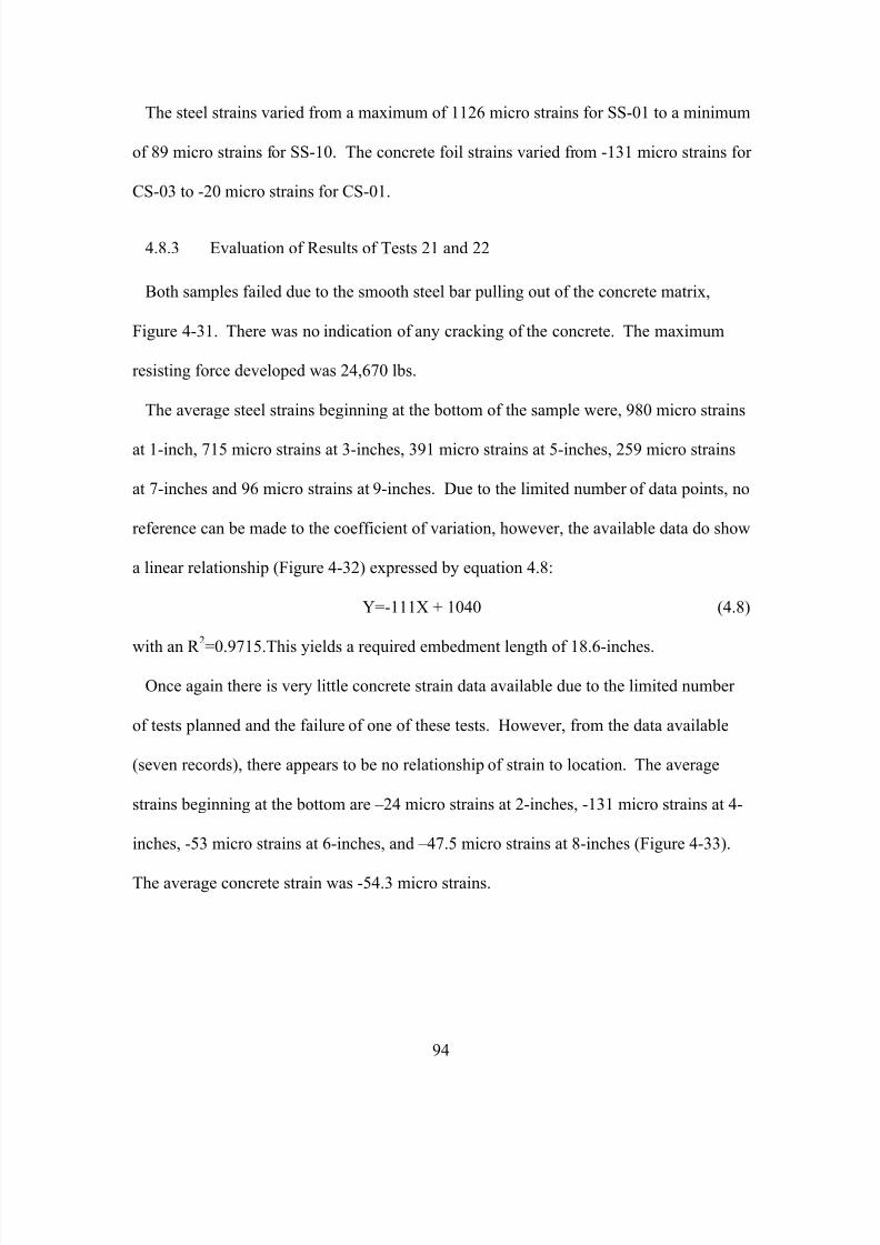
7/28/2019 Weathersby Dis
http://slidepdf.com/reader/full/weathersby-dis 111/280
94
The steel strains varied from a maximum of 1126 micro strains for SS-01 to a minimum
of 89 micro strains for SS-10. The concrete foil strains varied from -131 micro strains for
CS-03 to -20 micro strains for CS-01.
4.8.3 Evaluation of Results of Tests 21 and 22
Both samples failed due to the smooth steel bar pulling out of the concrete matrix,
Figure 4-31. There was no indication of any cracking of the concrete. The maximum
resisting force developed was 24,670 lbs.
The average steel strains beginning at the bottom of the sample were, 980 micro strains
at 1-inch, 715 micro strains at 3-inches, 391 micro strains at 5-inches, 259 micro strains
at 7-inches and 96 micro strains at 9-inches. Due to the limited number of data points, no
reference can be made to the coefficient of variation, however, the available data do show
a linear relationship (Figure 4-32) expressed by equation 4.8:
Y=-111X + 1040 (4.8)
with an R
2
=0.9715.This yields a required embedment length of 18.6-inches.
Once again there is very little concrete strain data available due to the limited number
of tests planned and the failure of one of these tests. However, from the data available
(seven records), there appears to be no relationship of strain to location. The average
strains beginning at the bottom are –24 micro strains at 2-inches, -131 micro strains at 4-
inches, -53 micro strains at 6-inches, and –47.5 micro strains at 8-inches (Figure 4-33).
The average concrete strain was -54.3 micro strains.
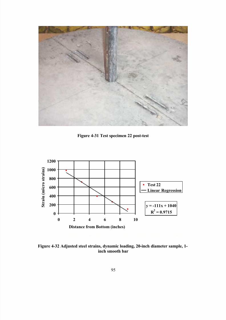
7/28/2019 Weathersby Dis
http://slidepdf.com/reader/full/weathersby-dis 112/280
95
Figure 4-31 Test specimen 22 post-test
y = -111x + 1040
R 2
= 0.97150
200
400
600
800
1000
1200
0 2 4 6 8 10
Distance from Bottom (inches)
S t r a i n ( m i c r o s t r a i n s )
Test 22
Linear Regression
Figure 4-32 Adjusted steel strains, dynamic loading, 20-inch diameter sample, 1-
inch smooth bar
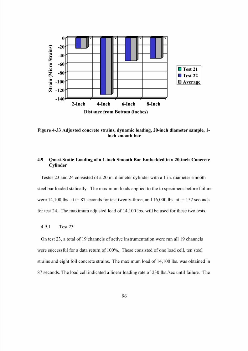
7/28/2019 Weathersby Dis
http://slidepdf.com/reader/full/weathersby-dis 113/280
96
-140
-120
-100
-80
-60
-40
-20
0
S t r a i n ( M i c r o S t r a i n s )
2-Inch 4-Inch 6-Inch 8-Inch
Distance from Bottom (inches)
Test 21
Test 22
Average
Figure 4-33 Adjusted concrete strains, dynamic loading, 20-inch diameter sample, 1-
inch smooth bar
4.9 Quasi-Static Loading of a 1-inch Smooth Bar Embedded in a 20-inch Concrete
Cylinder
Testes 23 and 24 consisted of a 20 in. diameter cylinder with a 1 in. diameter smooth
steel bar loaded statically. The maximum loads applied to the to specimens before failure
were 14,100 lbs. at t= 87 seconds for test twenty-three, and 16,000 lbs. at t= 152 seconds
for test 24. The maximum adjusted load of 14,100 lbs. will be used for these two tests.
4.9.1 Test 23
On test 23, a total of 19 channels of active instrumentation were run all 19 channels
were successful for a data return of 100%. These consisted of one load cell, ten steel
strains and eight foil concrete strains. The maximum load of 14,100 lbs. was obtained in
87 seconds. The load cell indicated a linear loading rate of 230 lbs./sec until failure. The
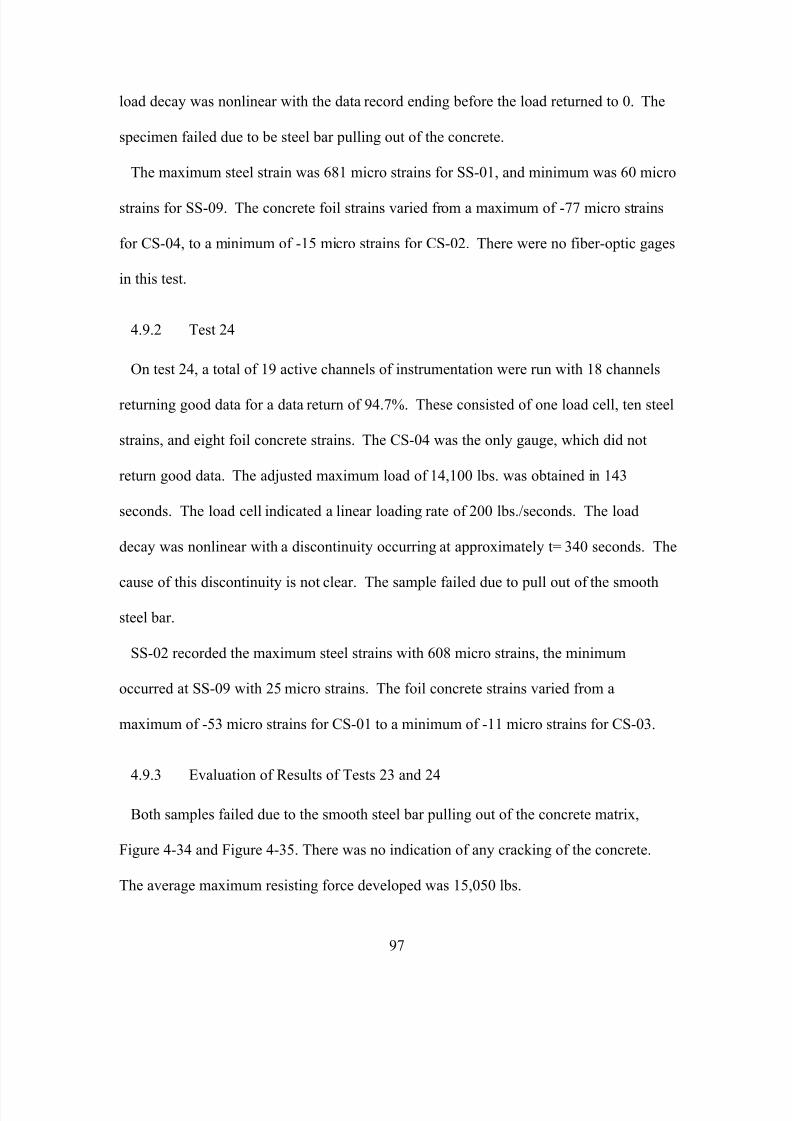
7/28/2019 Weathersby Dis
http://slidepdf.com/reader/full/weathersby-dis 114/280
97
load decay was nonlinear with the data record ending before the load returned to 0. The
specimen failed due to be steel bar pulling out of the concrete.
The maximum steel strain was 681 micro strains for SS-01, and minimum was 60 micro
strains for SS-09. The concrete foil strains varied from a maximum of -77 micro strains
for CS-04, to a minimum of -15 micro strains for CS-02. There were no fiber-optic gages
in this test.
4.9.2 Test 24
On test 24, a total of 19 active channels of instrumentation were run with 18 channels
returning good data for a data return of 94.7%. These consisted of one load cell, ten steel
strains, and eight foil concrete strains. The CS-04 was the only gauge, which did not
return good data. The adjusted maximum load of 14,100 lbs. was obtained in 143
seconds. The load cell indicated a linear loading rate of 200 lbs./seconds. The load
decay was nonlinear with a discontinuity occurring at approximately t= 340 seconds. The
cause of this discontinuity is not clear. The sample failed due to pull out of the smooth
steel bar.
SS-02 recorded the maximum steel strains with 608 micro strains, the minimum
occurred at SS-09 with 25 micro strains. The foil concrete strains varied from a
maximum of -53 micro strains for CS-01 to a minimum of -11 micro strains for CS-03.
4.9.3 Evaluation of Results of Tests 23 and 24
Both samples failed due to the smooth steel bar pulling out of the concrete matrix,
Figure 4-34 and Figure 4-35. There was no indication of any cracking of the concrete.
The average maximum resisting force developed was 15,050 lbs.
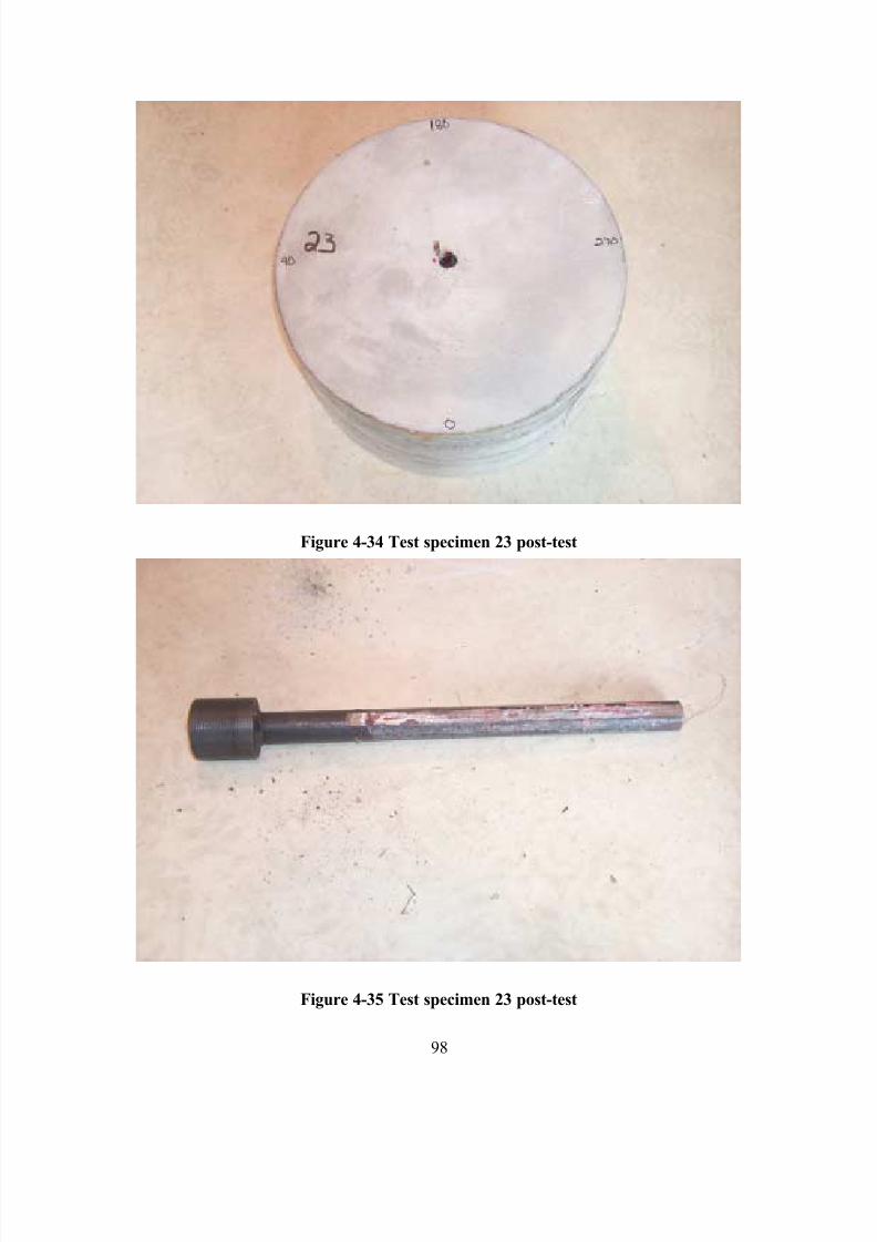
7/28/2019 Weathersby Dis
http://slidepdf.com/reader/full/weathersby-dis 115/280
98
Figure 4-34 Test specimen 23 post-test
Figure 4-35 Test specimen 23 post-test
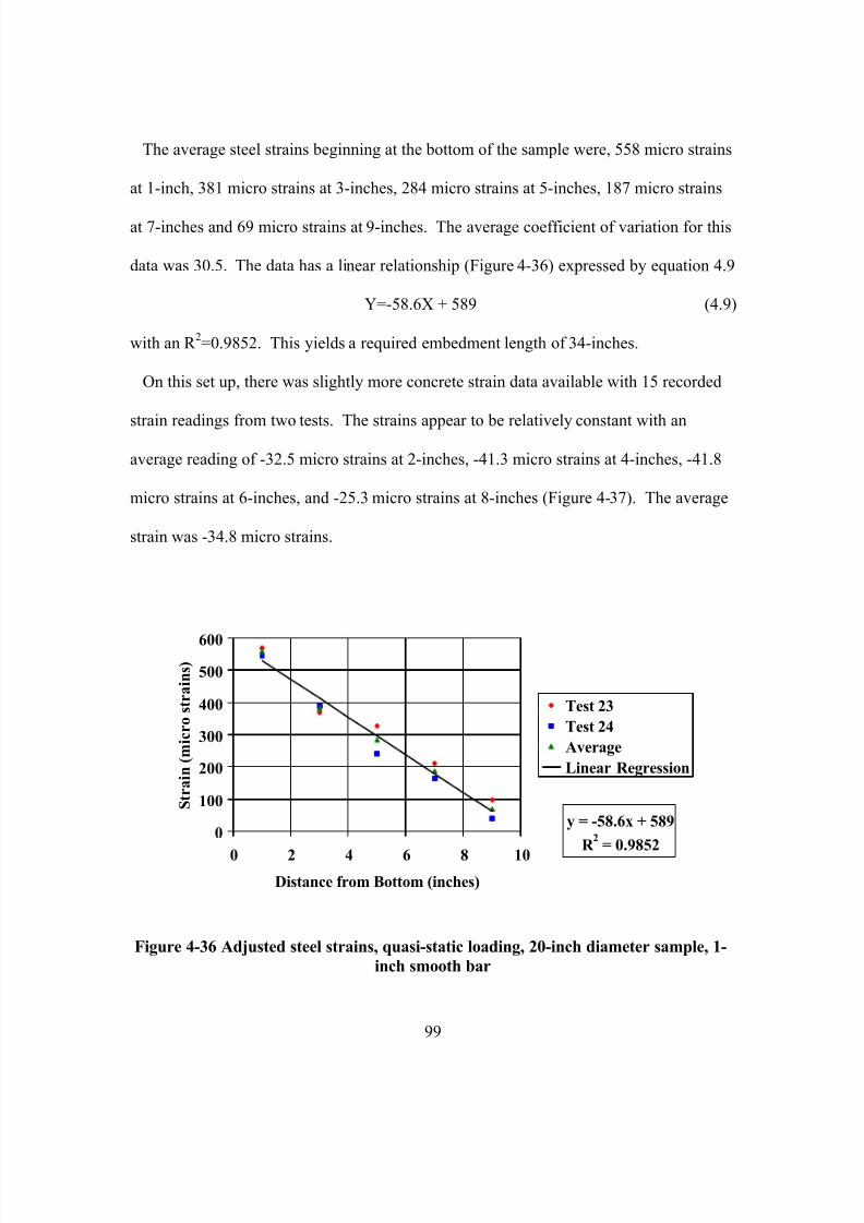
7/28/2019 Weathersby Dis
http://slidepdf.com/reader/full/weathersby-dis 116/280
99
The average steel strains beginning at the bottom of the sample were, 558 micro strains
at 1-inch, 381 micro strains at 3-inches, 284 micro strains at 5-inches, 187 micro strains
at 7-inches and 69 micro strains at 9-inches. The average coefficient of variation for this
data was 30.5. The data has a linear relationship (Figure 4-36) expressed by equation 4.9
Y=-58.6X + 589 (4.9)
with an R 2=0.9852. This yields a required embedment length of 34-inches.
On this set up, there was slightly more concrete strain data available with 15 recorded
strain readings from two tests. The strains appear to be relatively constant with an
average reading of -32.5 micro strains at 2-inches, -41.3 micro strains at 4-inches, -41.8
micro strains at 6-inches, and -25.3 micro strains at 8-inches (Figure 4-37). The average
strain was -34.8 micro strains.
y = -58.6x + 589
R 2
= 0.98520
100
200
300
400
500
600
0 2 4 6 8 10
Distance from Bottom (inches)
S t r a i n ( m i c r o s t r a i n s )
Test 23
Test 24
Average
Linear Regression
Figure 4-36 Adjusted steel strains, quasi-static loading, 20-inch diameter sample, 1-
inch smooth bar
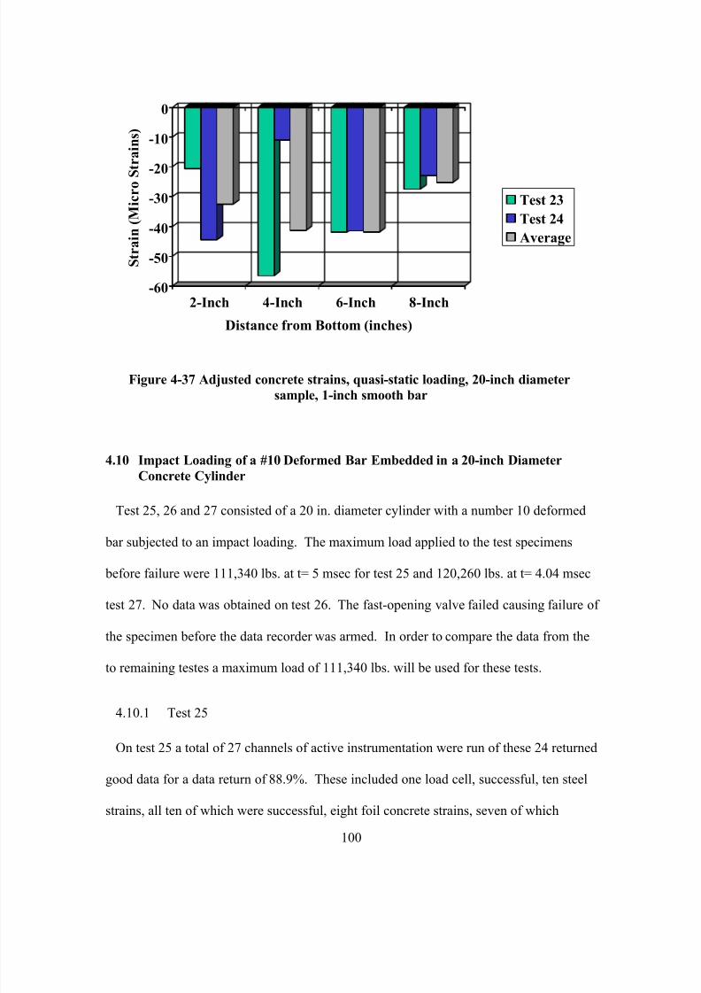
7/28/2019 Weathersby Dis
http://slidepdf.com/reader/full/weathersby-dis 117/280
100
-60
-50
-40
-30
-20
-10
0
S t r a i n ( M i c r o S
t r a i n s )
2-Inch 4-Inch 6-Inch 8-Inch
Distance from Bottom (inches)
Test 23
Test 24
Average
Figure 4-37 Adjusted concrete strains, quasi-static loading, 20-inch diameter
sample, 1-inch smooth bar
4.10 Impact Loading of a #10 Deformed Bar Embedded in a 20-inch Diameter
Concrete Cylinder
Test 25, 26 and 27 consisted of a 20 in. diameter cylinder with a number 10 deformed
bar subjected to an impact loading. The maximum load applied to the test specimens
before failure were 111,340 lbs. at t= 5 msec for test 25 and 120,260 lbs. at t= 4.04 msec
test 27. No data was obtained on test 26. The fast-opening valve failed causing failure of
the specimen before the data recorder was armed. In order to compare the data from the
to remaining testes a maximum load of 111,340 lbs. will be used for these tests.
4.10.1 Test 25
On test 25 a total of 27 channels of active instrumentation were run of these 24 returned
good data for a data return of 88.9%. These included one load cell, successful, ten steel
strains, all ten of which were successful, eight foil concrete strains, seven of which
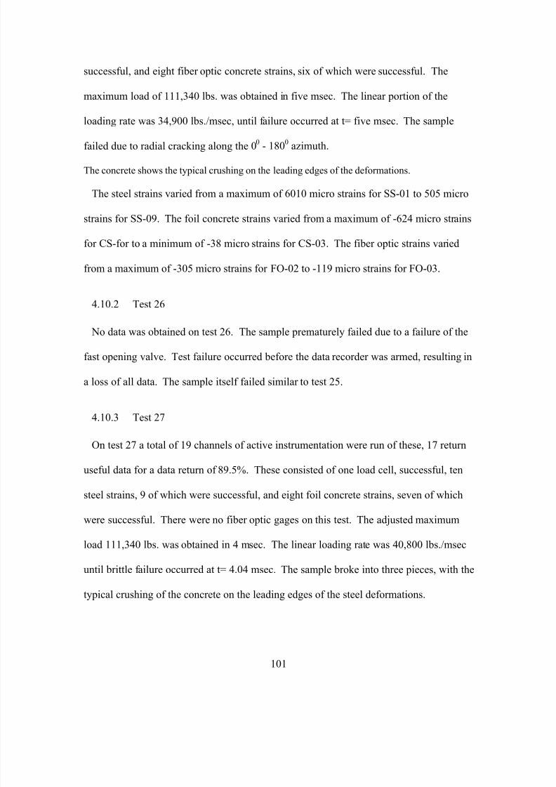
7/28/2019 Weathersby Dis
http://slidepdf.com/reader/full/weathersby-dis 118/280
101
successful, and eight fiber optic concrete strains, six of which were successful. The
maximum load of 111,340 lbs. was obtained in five msec. The linear portion of the
loading rate was 34,900 lbs./msec, until failure occurred at t= five msec. The sample
failed due to radial cracking along the 00
- 1800
azimuth.
The concrete shows the typical crushing on the leading edges of the deformations.
The steel strains varied from a maximum of 6010 micro strains for SS-01 to 505 micro
strains for SS-09. The foil concrete strains varied from a maximum of -624 micro strains
for CS-for to a minimum of -38 micro strains for CS-03. The fiber optic strains varied
from a maximum of -305 micro strains for FO-02 to -119 micro strains for FO-03.
4.10.2 Test 26
No data was obtained on test 26. The sample prematurely failed due to a failure of the
fast opening valve. Test failure occurred before the data recorder was armed, resulting in
a loss of all data. The sample itself failed similar to test 25.
4.10.3 Test 27
On test 27 a total of 19 channels of active instrumentation were run of these, 17 return
useful data for a data return of 89.5%. These consisted of one load cell, successful, ten
steel strains, 9 of which were successful, and eight foil concrete strains, seven of which
were successful. There were no fiber optic gages on this test. The adjusted maximum
load 111,340 lbs. was obtained in 4 msec. The linear loading rate was 40,800 lbs./msec
until brittle failure occurred at t= 4.04 msec. The sample broke into three pieces, with the
typical crushing of the concrete on the leading edges of the steel deformations.
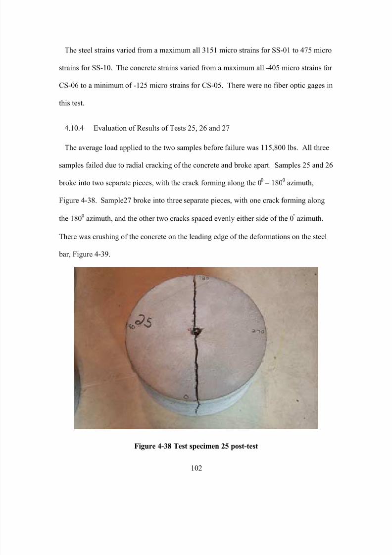
7/28/2019 Weathersby Dis
http://slidepdf.com/reader/full/weathersby-dis 119/280
102
The steel strains varied from a maximum all 3151 micro strains for SS-01 to 475 micro
strains for SS-10. The concrete strains varied from a maximum all -405 micro strains for
CS-06 to a minimum of -125 micro strains for CS-05. There were no fiber optic gages in
this test.
4.10.4 Evaluation of Results of Tests 25, 26 and 27
The average load applied to the two samples before failure was 115,800 lbs. All three
samples failed due to radial cracking of the concrete and broke apart. Samples 25 and 26
broke into two separate pieces, with the crack forming along the 00
– 1800
azimuth,
Figure 4-38. Sample27 broke into three separate pieces, with one crack forming along
the 1800
azimuth, and the other two cracks spaced evenly either side of the 0° azimuth.
There was crushing of the concrete on the leading edge of the deformations on the steel
bar, Figure 4-39.
Figure 4-38 Test specimen 25 post-test
7/28/2019 Weathersby Dis
http://slidepdf.com/reader/full/weathersby-dis 120/280
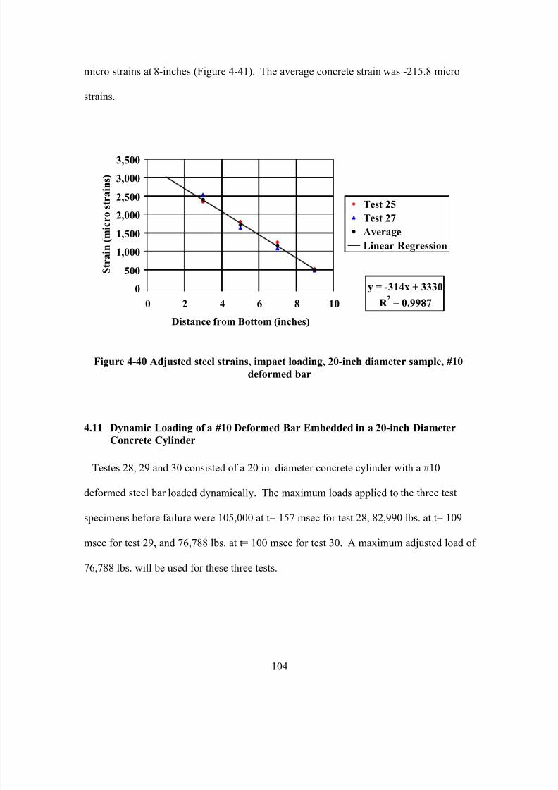
7/28/2019 Weathersby Dis
http://slidepdf.com/reader/full/weathersby-dis 121/280
104
micro strains at 8-inches (Figure 4-41). The average concrete strain was -215.8 micro
strains.
y = -314x + 3330
R 2
= 0.9987
0
500
1,000
1,500
2,000
2,500
3,000
3,500
0 2 4 6 8 10
Distance from Bottom (inches)
S t r a i n ( m i c r o s t r a i n s )
Test 25
Test 27
Average
Linear Regression
Figure 4-40 Adjusted steel strains, impact loading, 20-inch diameter sample, #10
deformed bar
4.11 Dynamic Loading of a #10 Deformed Bar Embedded in a 20-inch Diameter
Concrete Cylinder
Testes 28, 29 and 30 consisted of a 20 in. diameter concrete cylinder with a #10
deformed steel bar loaded dynamically. The maximum loads applied to the three test
specimens before failure were 105,000 at t= 157 msec for test 28, 82,990 lbs. at t= 109
msec for test 29, and 76,788 lbs. at t= 100 msec for test 30. A maximum adjusted load of
76,788 lbs. will be used for these three tests.
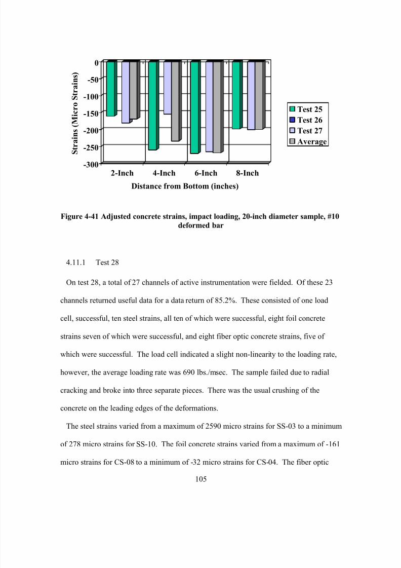
7/28/2019 Weathersby Dis
http://slidepdf.com/reader/full/weathersby-dis 122/280
105
-300
-250
-200
-150
-100
-50
0
S t r a i n s ( M i c r o S
t r a i n s )
2-Inch 4-Inch 6-Inch 8-Inch
Distance from Bottom (inches)
Test 25
Test 26
Test 27
Average
Figure 4-41 Adjusted concrete strains, impact loading, 20-inch diameter sample, #10
deformed bar
4.11.1 Test 28
On test 28, a total of 27 channels of active instrumentation were fielded. Of these 23
channels returned useful data for a data return of 85.2%. These consisted of one load
cell, successful, ten steel strains, all ten of which were successful, eight foil concrete
strains seven of which were successful, and eight fiber optic concrete strains, five of
which were successful. The load cell indicated a slight non-linearity to the loading rate,
however, the average loading rate was 690 lbs./msec. The sample failed due to radial
cracking and broke into three separate pieces. There was the usual crushing of the
concrete on the leading edges of the deformations.
The steel strains varied from a maximum of 2590 micro strains for SS-03 to a minimum
of 278 micro strains for SS-10. The foil concrete strains varied from a maximum of -161
micro strains for CS-08 to a minimum of -32 micro strains for CS-04. The fiber optic
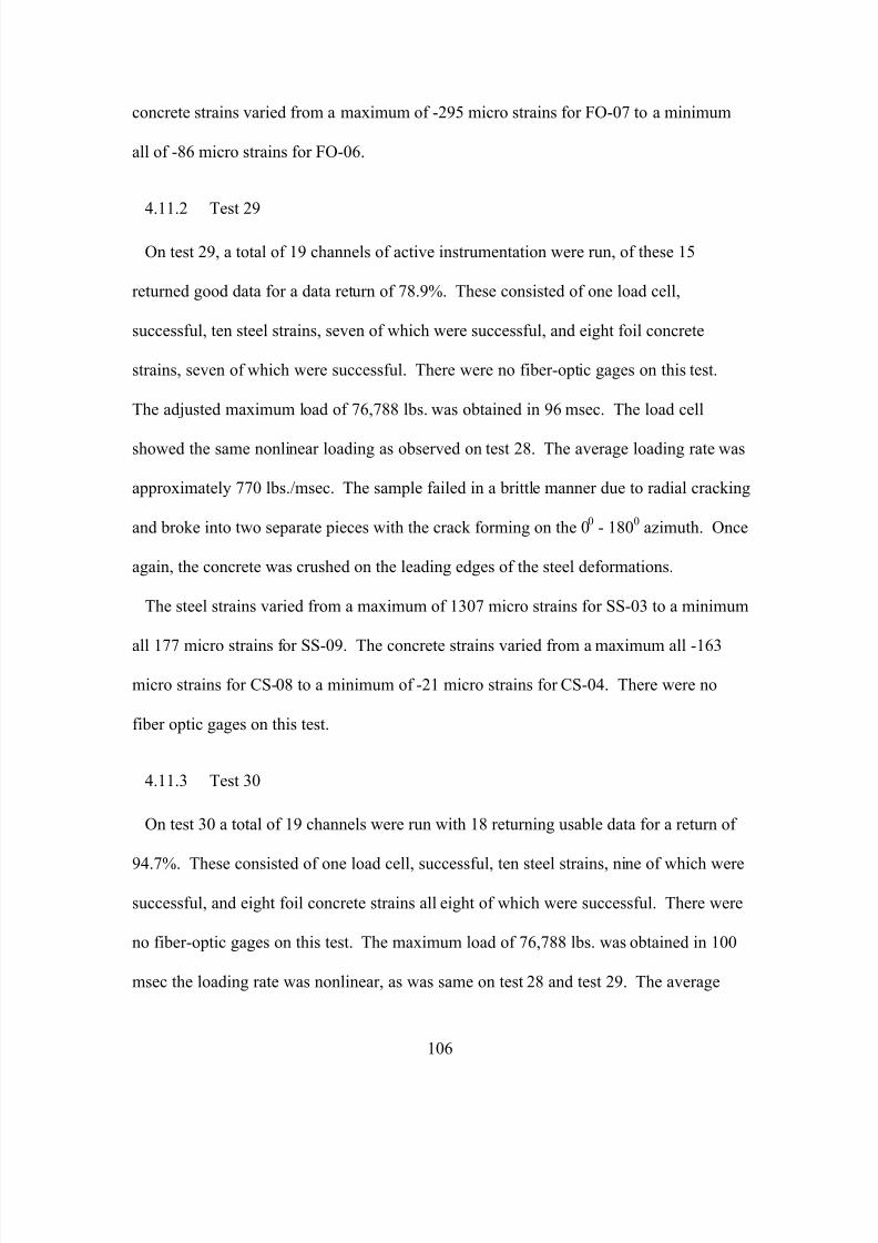
7/28/2019 Weathersby Dis
http://slidepdf.com/reader/full/weathersby-dis 123/280
106
concrete strains varied from a maximum of -295 micro strains for FO-07 to a minimum
all of -86 micro strains for FO-06.
4.11.2 Test 29
On test 29, a total of 19 channels of active instrumentation were run, of these 15
returned good data for a data return of 78.9%. These consisted of one load cell,
successful, ten steel strains, seven of which were successful, and eight foil concrete
strains, seven of which were successful. There were no fiber-optic gages on this test.
The adjusted maximum load of 76,788 lbs. was obtained in 96 msec. The load cell
showed the same nonlinear loading as observed on test 28. The average loading rate was
approximately 770 lbs./msec. The sample failed in a brittle manner due to radial cracking
and broke into two separate pieces with the crack forming on the 00
- 1800
azimuth. Once
again, the concrete was crushed on the leading edges of the steel deformations.
The steel strains varied from a maximum of 1307 micro strains for SS-03 to a minimum
all 177 micro strains for SS-09. The concrete strains varied from a maximum all -163
micro strains for CS-08 to a minimum of -21 micro strains for CS-04. There were no
fiber optic gages on this test.
4.11.3 Test 30
On test 30 a total of 19 channels were run with 18 returning usable data for a return of
94.7%. These consisted of one load cell, successful, ten steel strains, nine of which were
successful, and eight foil concrete strains all eight of which were successful. There were
no fiber-optic gages on this test. The maximum load of 76,788 lbs. was obtained in 100
msec the loading rate was nonlinear, as was same on test 28 and test 29. The average
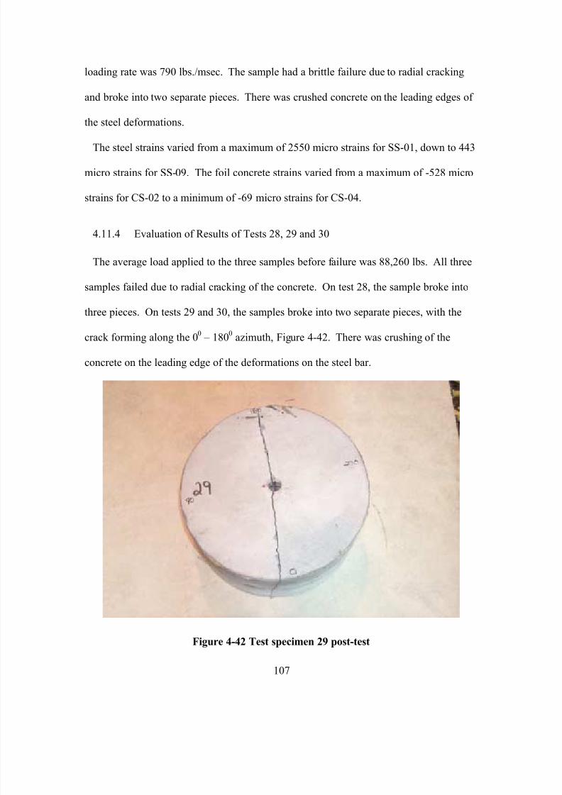
7/28/2019 Weathersby Dis
http://slidepdf.com/reader/full/weathersby-dis 124/280
107
loading rate was 790 lbs./msec. The sample had a brittle failure due to radial cracking
and broke into two separate pieces. There was crushed concrete on the leading edges of
the steel deformations.
The steel strains varied from a maximum of 2550 micro strains for SS-01, down to 443
micro strains for SS-09. The foil concrete strains varied from a maximum of -528 micro
strains for CS-02 to a minimum of -69 micro strains for CS-04.
4.11.4 Evaluation of Results of Tests 28, 29 and 30
The average load applied to the three samples before failure was 88,260 lbs. All three
samples failed due to radial cracking of the concrete. On test 28, the sample broke into
three pieces. On tests 29 and 30, the samples broke into two separate pieces, with the
crack forming along the 00
– 1800
azimuth, Figure 4-42. There was crushing of the
concrete on the leading edge of the deformations on the steel bar.
Figure 4-42 Test specimen 29 post-test
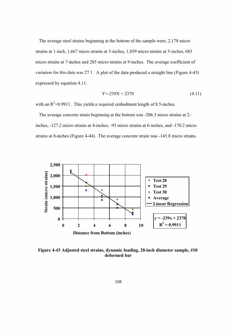
7/28/2019 Weathersby Dis
http://slidepdf.com/reader/full/weathersby-dis 125/280
108
The average steel strains beginning at the bottom of the sample were, 2,178 micro
strains at 1-inch, 1,667 micro strains at 3-inches, 1,059 micro strains at 5-inches, 683
micro strains at 7-inches and 285 micro strains at 9-inches. The average coefficient of
variation for this data was 27.1. A plot of the data produced a straight line (Figure 4-43)
expressed by equation 4.11:
Y=-239X + 2370 (4.11)
with an R 2=0.9911. This yields a required embedment length of 8.5-inches.
The average concrete strain beginning at the bottom was -206.3 micro strains at 2-
inches, -127.2 micro strains at 4-inches, -93 micro strains at 6-inches, and -170.2 micro
strains at 8-inches (Figure 4-44). The average concrete strain was -145.8 micro strains.
y = -239x + 2370
R 2
= 0.9911
0
500
1,000
1,500
2,000
2,500
0 2 4 6 8 10
Distance from Bottom (inches)
S t r a i n ( m i c r o s t r a i n
s )
Test 28
Test 29
Test 30
Average
Linear Regression
Figure 4-43 Adjusted steel strains, dynamic loading, 20-inch diameter sample, #10
deformed bar
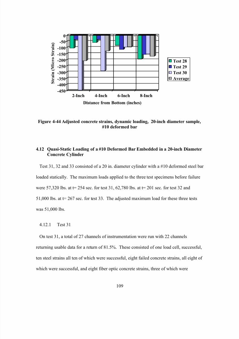
7/28/2019 Weathersby Dis
http://slidepdf.com/reader/full/weathersby-dis 126/280
109
-450
-400
-350
-300
-250
-200
-150
-100
-50
0
S t r a i n ( M i c r o
S t r a i n )
2-Inch 4-Inch 6-Inch 8-Inch
Distance from Bottom (inches)
Test 28
Test 29
Test 30
Average
Figure 4-44 Adjusted concrete strains, dynamic loading, 20-inch diameter sample,
#10 deformed bar
4.12 Quasi-Static Loading of a #10 Deformed Bar Embedded in a 20-inch Diameter
Concrete Cylinder
Test 31, 32 and 33 consisted of a 20 in. diameter cylinder with a #10 deformed steel bar
loaded statically. The maximum loads applied to the three test specimens before failure
were 57,320 lbs. at t= 254 sec. for test 31, 62,780 lbs. at t= 201 sec. for test 32 and
51,000 lbs. at t= 267 sec. for test 33. The adjusted maximum load for these three tests
was 51,000 lbs.
4.12.1 Test 31
On test 31, a total of 27 channels of instrumentation were run with 22 channels
returning usable data for a return of 81.5%. These consisted of one load cell, successful,
ten steel strains all ten of which were successful, eight failed concrete strains, all eight of
which were successful, and eight fiber optic concrete strains, three of which were
7/28/2019 Weathersby Dis
http://slidepdf.com/reader/full/weathersby-dis 127/280
110
successful. The load cell indicated a linear loading rate of 240 lbs./msec until failure.
The specimens failed due to radial cracking along the 00
– 1800
azimuth. The steel bar
indicated the common crushing of the concrete on the leading edges of the deformations.
The steel strains varied from a maximum of 4248 micro strains for SS-01 to a minimum
of 171 micro strains for SS-10. The foil concrete strains varied from a maximum of -183
micro strains for CS-02 to a minimum of -24 micro strains for CS-05. The fiber-optic
concrete strains varied from a maximum all of -129 micro strains for FO-03 to a
minimum of -98 micro strains for FO-07.
4.12.2 Test 32
On test 32, a total of 19 channels of instrumentation were run with 18 channels
returning usable data for a data return of 94.7 percent. These consisted of one load cell,
successful, ten steel strains, all ten of which were successful, and eight foil concrete
strains, seven of which were successful. There were no fiber optic gages on this test.
The adjusted maximum load of 51,000 lbs. was obtained in 150 sec. The load cell
indicated a linear loading rate of 250 lbs./msec. The failure of test specimens 32 was
similar to that of test 31 with the common radial cracking occurring along the 00
- 1800
azimuth and crushing of the concrete on the leading edges of the steel deformations.
The steel strains varied from a maximum of 1164 micro strains for SS-01 to a minimum
of 128 micro strains for SS-09. The concrete strains varied from a maximum of -145
micro strains for CS-04 to a minimum of -49 micro strains for CS-07.
7/28/2019 Weathersby Dis
http://slidepdf.com/reader/full/weathersby-dis 128/280
111
4.12.3 Test 33
On test 33, 19 channels of active instrumentation were run with 17 channels returning
usable data for a return of 89.5%. These consisted of one load cell, successful, ten steel
strains, eight of which were successful, and eight foil concrete strains, all eight of which
were successful. There were no fiber optic gages on this test. The maximum load of
51,000 lbs. was obtained in 267 sec. The load cell indicated a linear loading of 250
lbs./msec. The specimens failed in the same manner as on test 31 and 32.
The steel strains varied from a maximum of 3400 micro strains for SS-01 to a minimum
all of 175 micro strains for SS-09. The Foil concrete strains varied from a maximum of -
150 micro strains for CS-05 to a minimum of -15 micro strains for CS-04.
4.12.4 Evaluation of Results of Tests 31, 32 and 33
The average load applied to the three samples before failure was 57,000 lbs. All three
samples failed due to radial cracking of the concrete and broke into two separate pieces,
with the crack forming roughly along the 00
– 1800
azimuth, Figure 4-45. There was
crushing of the concrete on the leading edge of the deformations on the steel bar.
The average steel strains beginning at the bottom of the sample were, 2,233 micro
strains at 1-inch, 1,014 micro strains at 3-inches, 703 micro strains at 5-inches, 412 micro
strains at 7-inches and 191 micro strains at 9-inches. If we disregard the strain data from
the 1-inch position, where some strain readings were clearly in the plastic range, we get
an average coefficient of variation for this data of 17.9 and a linear relationship (Figure
4-46) expressed by equation 4.12
Y=-138X + 1410 (4.12)
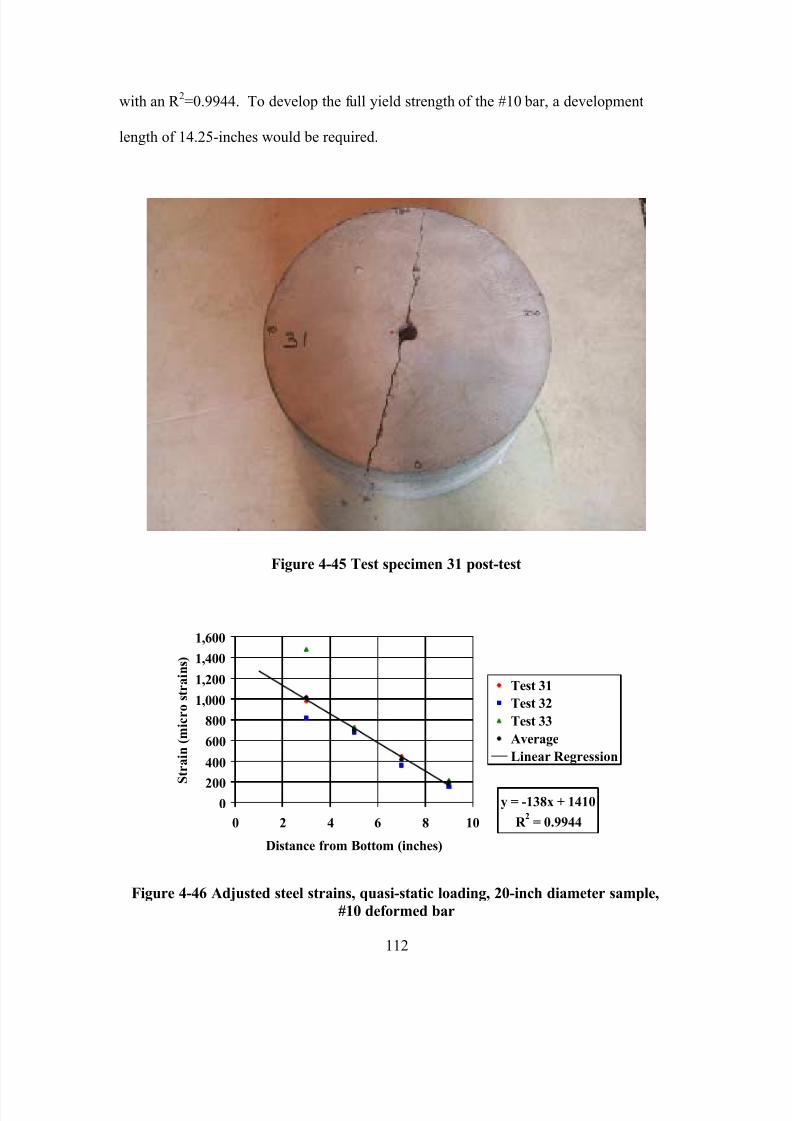
7/28/2019 Weathersby Dis
http://slidepdf.com/reader/full/weathersby-dis 129/280
112
with an R 2=0.9944. To develop the full yield strength of the #10 bar, a development
length of 14.25-inches would be required.
Figure 4-45 Test specimen 31 post-test
y = -138x + 1410
R 2
= 0.9944
0200
400
600
800
1,000
1,200
1,400
1,600
0 2 4 6 8 10
Distance from Bottom (inches)
S t r a i n ( m i c r o s t r a i n s )
Test 31
Test 32
Test 33
Average
Linear Regression
Figure 4-46 Adjusted steel strains, quasi-static loading, 20-inch diameter sample,
#10 deformed bar
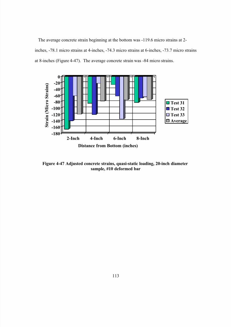
7/28/2019 Weathersby Dis
http://slidepdf.com/reader/full/weathersby-dis 130/280
113
The average concrete strain beginning at the bottom was -119.6 micro strains at 2-
inches, -78.1 micro strains at 4-inches, -74.3 micro strains at 6-inches, -73.7 micro strains
at 8-inches (Figure 4-47). The average concrete strain was -84 micro strains.
-180
-160
-140-120
-100
-80
-60
-40
-20
0
S t r a i n ( M i c r o S t r a i n s )
2-Inch 4-Inch 6-Inch 8-Inch
Distance from Bottom (inches)
Test 31
Test 32
Test 33Average
Figure 4-47 Adjusted concrete strains, quasi-static loading, 20-inch diameter
sample, #10 deformed bar
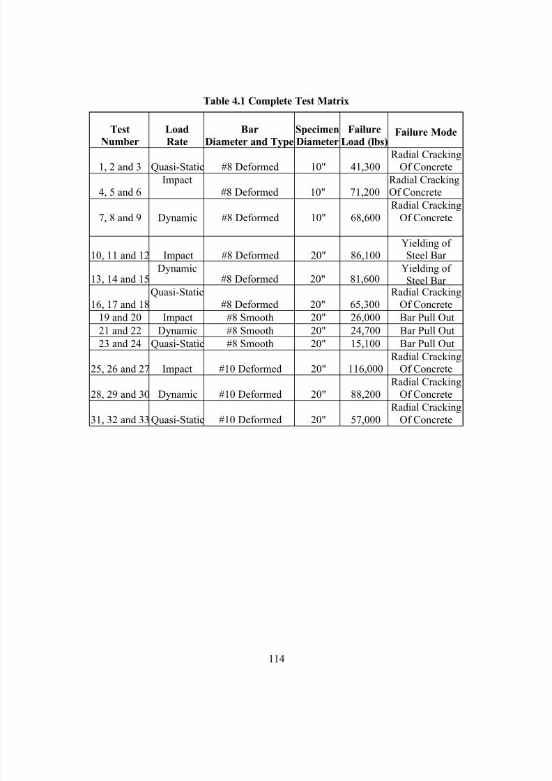
7/28/2019 Weathersby Dis
http://slidepdf.com/reader/full/weathersby-dis 131/280
114
Table 4.1 Complete Test Matrix
Test
Number
Load
Rate
Bar
Diameter and Type
Specimen
Diameter
Failure
Load (lbs) Failure Mode
1, 2 and 3 Quasi-Static #8 Deformed 10" 41,300
Radial Cracking
Of Concrete
4, 5 and 6Impact
#8 Deformed 10" 71,200Radial CrackingOf Concrete
7, 8 and 9 Dynamic #8 Deformed 10" 68,600
Radial Cracking
Of Concrete
10, 11 and 12 Impact #8 Deformed 20" 86,100Yielding of Steel Bar
13, 14 and 15 Dynamic #8 Deformed 20" 81,600 Yielding of Steel Bar
16, 17 and 18
Quasi-Static
#8 Deformed 20" 65,300
Radial Cracking
Of Concrete
19 and 20 Impact #8 Smooth 20" 26,000 Bar Pull Out
21 and 22 Dynamic #8 Smooth 20" 24,700 Bar Pull Out
23 and 24 Quasi-Static #8 Smooth 20" 15,100 Bar Pull Out
25, 26 and 27 Impact #10 Deformed 20" 116,000Radial Cracking
Of Concrete
28, 29 and 30 Dynamic #10 Deformed 20" 88,200
Radial Cracking
Of Concrete
31, 32 and 33 Quasi-Static #10 Deformed 20" 57,000Radial Cracking
Of Concrete
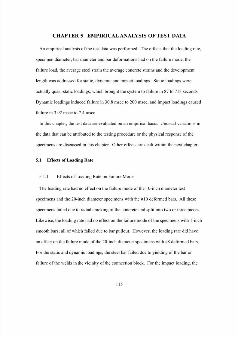
7/28/2019 Weathersby Dis
http://slidepdf.com/reader/full/weathersby-dis 132/280
115
CHAPTER 5 EMPIRICAL ANALYSIS OF TEST DATA
An empirical analysis of the test data was performed. The effects that the loading rate,
specimen diameter, bar diameter and bar deformations had on the failure mode, the
failure load, the average steel strain the average concrete strains and the development
length was addressed for static, dynamic and impact loadings. Static loadings were
actually quasi-static loadings, which brought the system to failure in 87 to 713 seconds.
Dynamic loadings induced failure in 30.8 msec to 200 msec, and impact loadings caused
failure in 3.92 msec to 7.4 msec.
In this chapter, the test data are evaluated on an empirical basis. Unusual variations in
the data that can be attributed to the testing procedure or the physical response of the
specimens are discussed in this chapter. Other effects are dealt within the next chapter.
5.1 Effects of Loading Rate
5.1.1 Effects of Loading Rate on Failure Mode
The loading rate had no effect on the failure mode of the 10-inch diameter test
specimens and the 20-inch diameter specimens with the #10 deformed bars. All these
specimens failed due to radial cracking of the concrete and split into two or three pieces.
Likewise, the loading rate had no effect on the failure mode of the specimens with 1-inch
smooth bars; all of which failed due to bar pullout. However, the loading rate did have
an effect on the failure mode of the 20-inch diameter specimens with #8 deformed bars.
For the static and dynamic loadings, the steel bar failed due to yielding of the bar or
failure of the welds in the vicinity of the connection block. For the impact loading, the
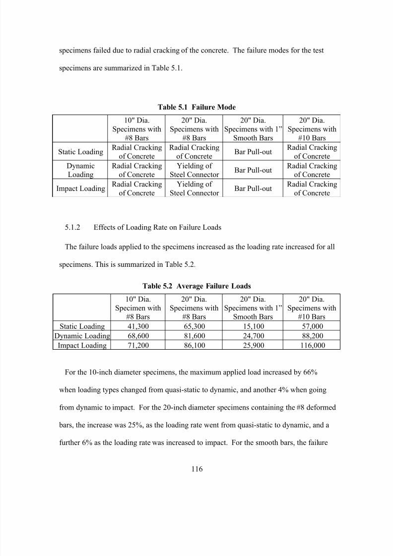
7/28/2019 Weathersby Dis
http://slidepdf.com/reader/full/weathersby-dis 133/280
116
specimens failed due to radial cracking of the concrete. The failure modes for the test
specimens are summarized in Table 5.1.
Table 5.1 Failure Mode
10" Dia.
Specimens with
#8 Bars
20" Dia.
Specimens with
#8 Bars
20" Dia.
Specimens with 1”
Smooth Bars
20" Dia.
Specimens with
#10 Bars
Static LoadingRadial Cracking
of ConcreteRadial Cracking
of ConcreteBar Pull-out
Radial Cracking
of Concrete
DynamicLoading
Radial Crackingof Concrete
Yielding of Steel Connector
Bar Pull-outRadial Cracking
of Concrete
Impact LoadingRadial Cracking
of Concrete
Yielding of
Steel Connector
Bar Pull-outRadial Cracking
of Concrete
5.1.2 Effects of Loading Rate on Failure Loads
The failure loads applied to the specimens increased as the loading rate increased for all
specimens. This is summarized in Table 5.2.
Table 5.2 Average Failure Loads
10" Dia.
Specimen with#8 Bars
20" Dia.
Specimens with#8 Bars
20" Dia.
Specimens with 1”Smooth Bars
20" Dia.
Specimens with#10 Bars
Static Loading 41,300 65,300 15,100 57,000
Dynamic Loading 68,600 81,600 24,700 88,200
Impact Loading 71,200 86,100 25,900 116,000
For the 10-inch diameter specimens, the maximum applied load increased by 66%
when loading types changed from quasi-static to dynamic, and another 4% when going
from dynamic to impact. For the 20-inch diameter specimens containing the #8 deformed
bars, the increase was 25%, as the loading rate went from quasi-static to dynamic, and a
further 6% as the loading rate was increased to impact. For the smooth bars, the failure
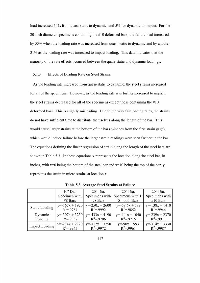
7/28/2019 Weathersby Dis
http://slidepdf.com/reader/full/weathersby-dis 134/280
117
load increased 64% from quasi-static to dynamic, and 5% for dynamic to impact. For the
20-inch diameter specimens containing the #10 deformed bars, the failure load increased
by 55% when the loading rate was increased from quasi-static to dynamic and by another
31% as the loading rate was increased to impact loading. This data indicates that the
majority of the rate effects occurred between the quasi-static and dynamic loadings.
5.1.3 Effects of Loading Rate on Steel Strains
As the loading rate increased from quasi-static to dynamic, the steel strains increased
for all of the specimens. However, as the loading rate was further increased to impact,
the steel strains decreased for all of the specimens except those containing the #10
deformed bars. This is slightly misleading. Due to the very fast loading rates, the strains
do not have sufficient time to distribute themselves along the length of the bar. This
would cause larger strains at the bottom of the bar (6-inches from the first strain gage),
which would induce failure before the larger strain readings were seen farther up the bar.
The equations defining the linear regression of strain along the length of the steel bars are
shown in Table 5.3. In these equations x represents the location along the steel bar, in
inches, with x=0 being the bottom of the steel bar and x=10 being the top of the bar; y
represents the strain in micro strains at location x.
Table 5.3 Average Steel Strains at Failure
10" Dia.
Specimen with
#8 Bars
20" Dia.
Specimens with
#8 Bars
20" Dia.
Specimens with 1”
Smooth Bars
20" Dia.
Specimens with
#10 Bars
Static Loadingy=-167x + 1920
R 2=.9784
y=-250x + 2600R
2=.9992
y=-58.6x + 589R
2=.9852
y=-138x + 1410R
2=.9944
DynamicLoading
y=-307x + 3230R
2=.9837
y=-433x + 4190R
2=.9706
y=-111x + 1040R
2=.9715
y=-239x + 2370R
2=.9911
Impact Loadingy=-274x + 2720
R 2=.9945
y=-312x + 3250
R 2=.9972
y=-90x + 993
R 2=.9961
y=-314x + 3330
R 2=.9987
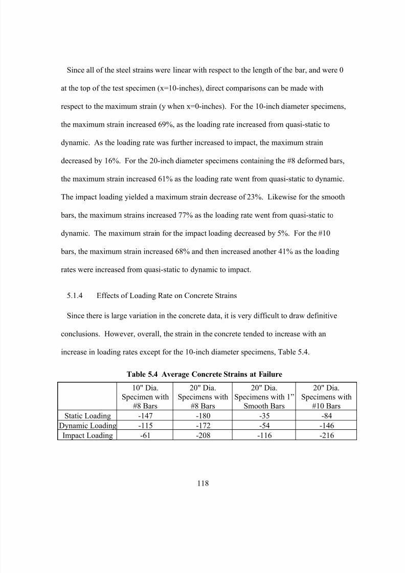
7/28/2019 Weathersby Dis
http://slidepdf.com/reader/full/weathersby-dis 135/280
118
Since all of the steel strains were linear with respect to the length of the bar, and were 0
at the top of the test specimen (x=10-inches), direct comparisons can be made with
respect to the maximum strain (y when x=0-inches). For the 10-inch diameter specimens,
the maximum strain increased 69%, as the loading rate increased from quasi-static to
dynamic. As the loading rate was further increased to impact, the maximum strain
decreased by 16%. For the 20-inch diameter specimens containing the #8 deformed bars,
the maximum strain increased 61% as the loading rate went from quasi-static to dynamic.
The impact loading yielded a maximum strain decrease of 23%. Likewise for the smooth
bars, the maximum strains increased 77% as the loading rate went from quasi-static to
dynamic. The maximum strain for the impact loading decreased by 5%. For the #10
bars, the maximum strain increased 68% and then increased another 41% as the loading
rates were increased from quasi-static to dynamic to impact.
5.1.4 Effects of Loading Rate on Concrete Strains
Since there is large variation in the concrete data, it is very difficult to draw definitive
conclusions. However, overall, the strain in the concrete tended to increase with an
increase in loading rates except for the 10-inch diameter specimens, Table 5.4.
Table 5.4 Average Concrete Strains at Failure
10" Dia.
Specimen with
#8 Bars
20" Dia.
Specimens with
#8 Bars
20" Dia.
Specimens with 1”
Smooth Bars
20" Dia.
Specimens with
#10 Bars
Static Loading -147 -180 -35 -84
Dynamic Loading -115 -172 -54 -146
Impact Loading -61 -208 -116 -216
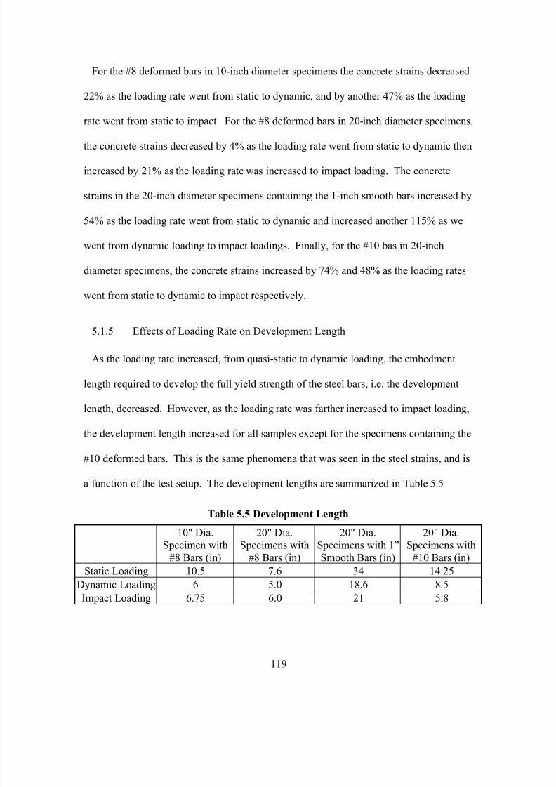
7/28/2019 Weathersby Dis
http://slidepdf.com/reader/full/weathersby-dis 136/280
119
For the #8 deformed bars in 10-inch diameter specimens the concrete strains decreased
22% as the loading rate went from static to dynamic, and by another 47% as the loading
rate went from static to impact. For the #8 deformed bars in 20-inch diameter specimens,
the concrete strains decreased by 4% as the loading rate went from static to dynamic then
increased by 21% as the loading rate was increased to impact loading. The concrete
strains in the 20-inch diameter specimens containing the 1-inch smooth bars increased by
54% as the loading rate went from static to dynamic and increased another 115% as we
went from dynamic loading to impact loadings. Finally, for the #10 bas in 20-inch
diameter specimens, the concrete strains increased by 74% and 48% as the loading rates
went from static to dynamic to impact respectively.
5.1.5 Effects of Loading Rate on Development Length
As the loading rate increased, from quasi-static to dynamic loading, the embedment
length required to develop the full yield strength of the steel bars, i.e. the development
length, decreased. However, as the loading rate was farther increased to impact loading,
the development length increased for all samples except for the specimens containing the
#10 deformed bars. This is the same phenomena that was seen in the steel strains, and is
a function of the test setup. The development lengths are summarized in Table 5.5
Table 5.5 Development Length
10" Dia.
Specimen with
#8 Bars (in)
20" Dia.
Specimens with
#8 Bars (in)
20" Dia.
Specimens with 1”
Smooth Bars (in)
20" Dia.
Specimens with
#10 Bars (in)
Static Loading 10.5 7.6 34 14.25
Dynamic Loading 6 5.0 18.6 8.5
Impact Loading 6.75 6.0 21 5.8
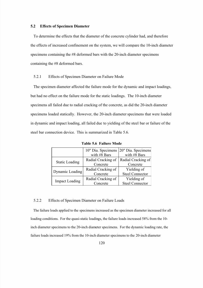
7/28/2019 Weathersby Dis
http://slidepdf.com/reader/full/weathersby-dis 137/280
120
5.2 Effects of Specimen Diameter
To determine the effects that the diameter of the concrete cylinder had, and therefore
the effects of increased confinement on the system, we will compare the 10-inch diameter
specimens containing the #8 deformed bars with the 20-inch diameter specimens
containing the #8 deformed bars.
5.2.1 Effects of Specimen Diameter on Failure Mode
The specimen diameter affected the failure mode for the dynamic and impact loadings,
but had no effect on the failure mode for the static loadings. The 10-inch diameter
specimens all failed due to radial cracking of the concrete, as did the 20-inch diameter
specimens loaded statically. However, the 20-inch diameter specimens that were loaded
in dynamic and impact loading, all failed due to yielding of the steel bar or failure of the
steel bar connection device. This is summarized in Table 5.6.
Table 5.6 Failure Mode
10" Dia. Specimenswith #8 Bars
20" Dia. Specimenswith #8 Bars
Static LoadingRadial Cracking of
Concrete
Radial Cracking of
Concrete
Dynamic LoadingRadial Cracking of
Concrete
Yielding of
Steel Connector
Impact LoadingRadial Cracking of
ConcreteYielding of
Steel Connector
5.2.2 Effects of Specimen Diameter on Failure Loads
The failure loads applied to the specimens increased as the specimen diameter increased for all
loading conditions. For the quasi-static loadings, the failure loads increased 58% from the 10-
inch diameter specimens to the 20-inch diameter specimens. For the dynamic loading rate, the
failure loads increased 19% from the 10-inch diameter specimens to the 20-inch diameter
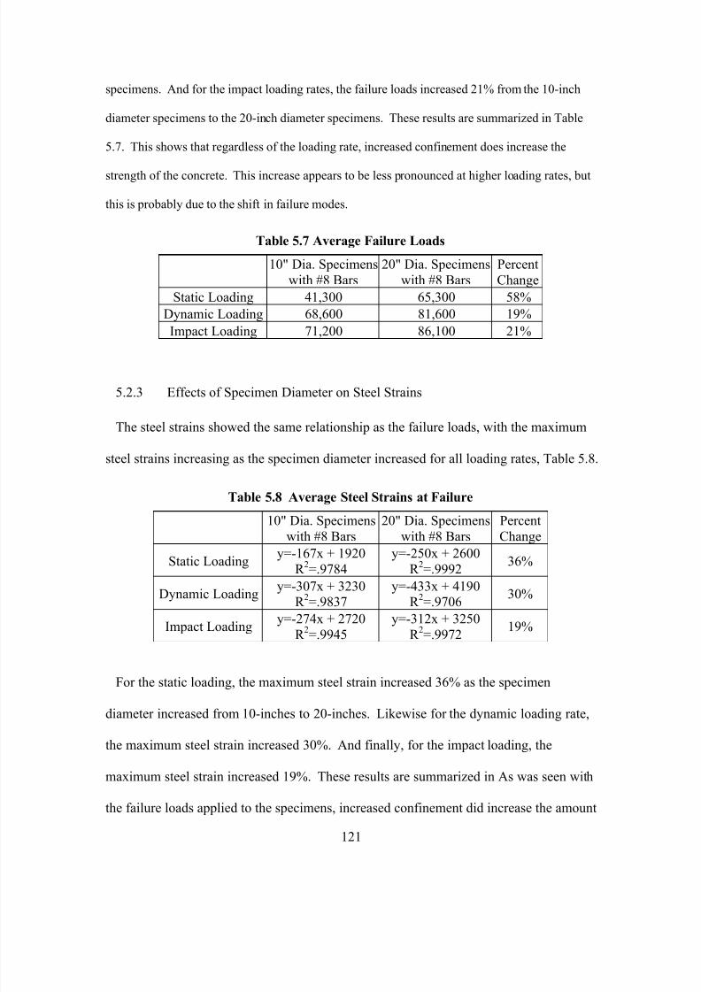
7/28/2019 Weathersby Dis
http://slidepdf.com/reader/full/weathersby-dis 138/280
121
specimens. And for the impact loading rates, the failure loads increased 21% from the 10-inch
diameter specimens to the 20-inch diameter specimens. These results are summarized in Table
5.7. This shows that regardless of the loading rate, increased confinement does increase the
strength of the concrete. This increase appears to be less pronounced at higher loading rates, but
this is probably due to the shift in failure modes.
Table 5.7 Average Failure Loads
10" Dia. Specimens
with #8 Bars
20" Dia. Specimens
with #8 Bars
Percent
Change
Static Loading 41,300 65,300 58%
Dynamic Loading 68,600 81,600 19%
Impact Loading 71,200 86,100 21%
5.2.3 Effects of Specimen Diameter on Steel Strains
The steel strains showed the same relationship as the failure loads, with the maximum
steel strains increasing as the specimen diameter increased for all loading rates, Table 5.8.
Table 5.8 Average Steel Strains at Failure
10" Dia. Specimenswith #8 Bars
20" Dia. Specimenswith #8 Bars
PercentChange
Static Loadingy=-167x + 1920
R 2=.9784
y=-250x + 2600
R 2=.9992
36%
Dynamic Loadingy=-307x + 3230
R 2=.9837
y=-433x + 4190R
2=.9706
30%
Impact Loadingy=-274x + 2720
R 2=.9945
y=-312x + 3250
R 2=.9972
19%
For the static loading, the maximum steel strain increased 36% as the specimen
diameter increased from 10-inches to 20-inches. Likewise for the dynamic loading rate,
the maximum steel strain increased 30%. And finally, for the impact loading, the
maximum steel strain increased 19%. These results are summarized in As was seen with
the failure loads applied to the specimens, increased confinement did increase the amount
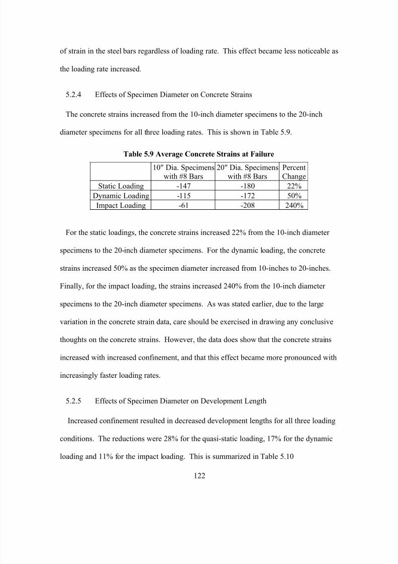
7/28/2019 Weathersby Dis
http://slidepdf.com/reader/full/weathersby-dis 139/280
122
of strain in the steel bars regardless of loading rate. This effect became less noticeable as
the loading rate increased.
5.2.4 Effects of Specimen Diameter on Concrete Strains
The concrete strains increased from the 10-inch diameter specimens to the 20-inch
diameter specimens for all three loading rates. This is shown in Table 5.9.
Table 5.9 Average Concrete Strains at Failure
10" Dia. Specimenswith #8 Bars
20" Dia. Specimenswith #8 Bars
PercentChange
Static Loading -147 -180 22%
Dynamic Loading -115 -172 50%Impact Loading -61 -208 240%
For the static loadings, the concrete strains increased 22% from the 10-inch diameter
specimens to the 20-inch diameter specimens. For the dynamic loading, the concrete
strains increased 50% as the specimen diameter increased from 10-inches to 20-inches.
Finally, for the impact loading, the strains increased 240% from the 10-inch diameter
specimens to the 20-inch diameter specimens. As was stated earlier, due to the large
variation in the concrete strain data, care should be exercised in drawing any conclusive
thoughts on the concrete strains. However, the data does show that the concrete strains
increased with increased confinement, and that this effect became more pronounced with
increasingly faster loading rates.
5.2.5 Effects of Specimen Diameter on Development Length
Increased confinement resulted in decreased development lengths for all three loading
conditions. The reductions were 28% for the quasi-static loading, 17% for the dynamic
loading and 11% for the impact loading. This is summarized in Table 5.10
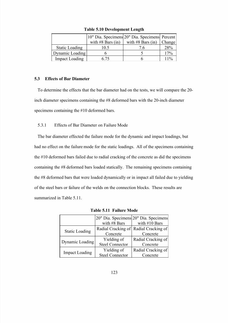
7/28/2019 Weathersby Dis
http://slidepdf.com/reader/full/weathersby-dis 140/280
123
Table 5.10 Development Length
10" Dia. Specimens
with #8 Bars (in)
20" Dia. Specimens
with #8 Bars (in)
Percent
Change
Static Loading 10.5 7.6 28%
Dynamic Loading 6 5 17%
Impact Loading 6.75 6 11%
5.3 Effects of Bar Diameter
To determine the effects that the bar diameter had on the tests, we will compare the 20-
inch diameter specimens containing the #8 deformed bars with the 20-inch diameter
specimens containing the #10 deformed bars.
5.3.1 Effects of Bar Diameter on Failure Mode
The bar diameter effected the failure mode for the dynamic and impact loadings, but
had no effect on the failure mode for the static loadings. All of the specimens containing
the #10 deformed bars failed due to radial cracking of the concrete as did the specimens
containing the #8 deformed bars loaded statically. The remaining specimens containing
the #8 deformed bars that were loaded dynamically or in impact all failed due to yielding
of the steel bars or failure of the welds on the connection blocks. These results are
summarized in Table 5.11.
Table 5.11 Failure Mode
20" Dia. Specimens
with #8 Bars
20" Dia. Specimens
with #10 Bars
Static LoadingRadial Cracking of
Concrete
Radial Cracking of
Concrete
Dynamic LoadingYielding of
Steel Connector Radial Cracking of
Concrete
Impact LoadingYielding of
Steel Connector
Radial Cracking of
Concrete
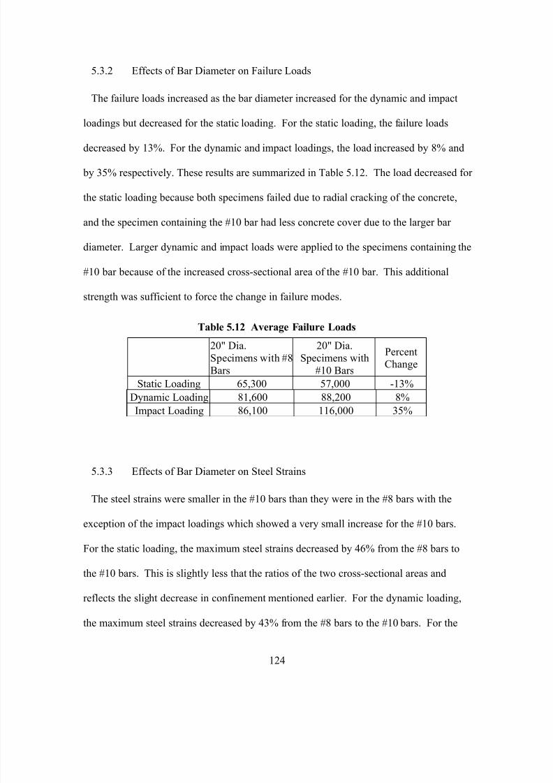
7/28/2019 Weathersby Dis
http://slidepdf.com/reader/full/weathersby-dis 141/280
124
5.3.2 Effects of Bar Diameter on Failure Loads
The failure loads increased as the bar diameter increased for the dynamic and impact
loadings but decreased for the static loading. For the static loading, the failure loads
decreased by 13%. For the dynamic and impact loadings, the load increased by 8% and
by 35% respectively. These results are summarized in Table 5.12. The load decreased for
the static loading because both specimens failed due to radial cracking of the concrete,
and the specimen containing the #10 bar had less concrete cover due to the larger bar
diameter. Larger dynamic and impact loads were applied to the specimens containing the
#10 bar because of the increased cross-sectional area of the #10 bar. This additional
strength was sufficient to force the change in failure modes.
Table 5.12 Average Failure Loads
20" Dia.
Specimens with #8
Bars
20" Dia.
Specimens with
#10 Bars
PercentChange
Static Loading 65,300 57,000 -13%
Dynamic Loading 81,600 88,200 8%
Impact Loading 86,100 116,000 35%
5.3.3 Effects of Bar Diameter on Steel Strains
The steel strains were smaller in the #10 bars than they were in the #8 bars with the
exception of the impact loadings which showed a very small increase for the #10 bars.
For the static loading, the maximum steel strains decreased by 46% from the #8 bars to
the #10 bars. This is slightly less that the ratios of the two cross-sectional areas and
reflects the slight decrease in confinement mentioned earlier. For the dynamic loading,
the maximum steel strains decreased by 43% from the #8 bars to the #10 bars. For the
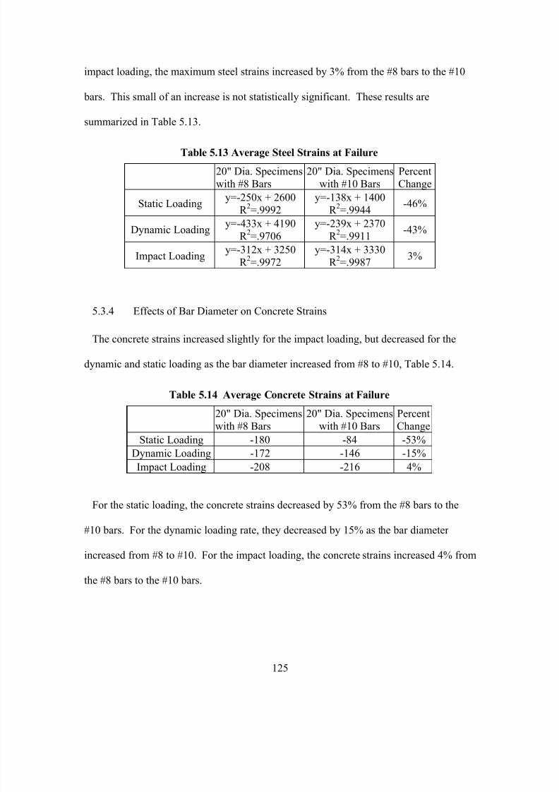
7/28/2019 Weathersby Dis
http://slidepdf.com/reader/full/weathersby-dis 142/280
125
impact loading, the maximum steel strains increased by 3% from the #8 bars to the #10
bars. This small of an increase is not statistically significant. These results are
summarized in Table 5.13.
Table 5.13 Average Steel Strains at Failure
20" Dia. Specimens
with #8 Bars
20" Dia. Specimens
with #10 Bars
Percent
Change
Static Loadingy=-250x + 2600
R 2=.9992
y=-138x + 1400
R 2=.9944
-46%
Dynamic Loadingy=-433x + 4190
R 2=.9706
y=-239x + 2370
R 2=.9911
-43%
Impact Loadingy=-312x + 3250
R 2=.9972
y=-314x + 3330
R 2=.9987
3%
5.3.4 Effects of Bar Diameter on Concrete Strains
The concrete strains increased slightly for the impact loading, but decreased for the
dynamic and static loading as the bar diameter increased from #8 to #10, Table 5.14.
Table 5.14 Average Concrete Strains at Failure
20" Dia. Specimenswith #8 Bars
20" Dia. Specimenswith #10 Bars
PercentChange
Static Loading -180 -84 -53%
Dynamic Loading -172 -146 -15%
Impact Loading -208 -216 4%
For the static loading, the concrete strains decreased by 53% from the #8 bars to the
#10 bars. For the dynamic loading rate, they decreased by 15% as the bar diameter
increased from #8 to #10. For the impact loading, the concrete strains increased 4% from
the #8 bars to the #10 bars.
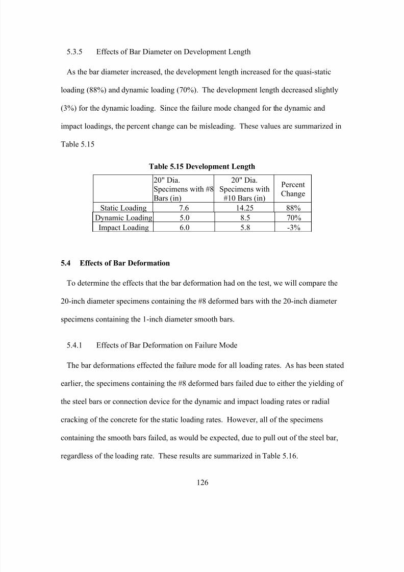
7/28/2019 Weathersby Dis
http://slidepdf.com/reader/full/weathersby-dis 143/280
126
5.3.5 Effects of Bar Diameter on Development Length
As the bar diameter increased, the development length increased for the quasi-static
loading (88%) and dynamic loading (70%). The development length decreased slightly
(3%) for the dynamic loading. Since the failure mode changed for the dynamic and
impact loadings, the percent change can be misleading. These values are summarized in
Table 5.15
Table 5.15 Development Length
20" Dia.Specimens with #8
Bars (in)
20" Dia.Specimens with
#10 Bars (in)
Percent
Change
Static Loading 7.6 14.25 88%
Dynamic Loading 5.0 8.5 70%
Impact Loading 6.0 5.8 -3%
5.4 Effects of Bar Deformation
To determine the effects that the bar deformation had on the test, we will compare the
20-inch diameter specimens containing the #8 deformed bars with the 20-inch diameter
specimens containing the 1-inch diameter smooth bars.
5.4.1 Effects of Bar Deformation on Failure Mode
The bar deformations effected the failure mode for all loading rates. As has been stated
earlier, the specimens containing the #8 deformed bars failed due to either the yielding of
the steel bars or connection device for the dynamic and impact loading rates or radial
cracking of the concrete for the static loading rates. However, all of the specimens
containing the smooth bars failed, as would be expected, due to pull out of the steel bar,
regardless of the loading rate. These results are summarized in Table 5.16.
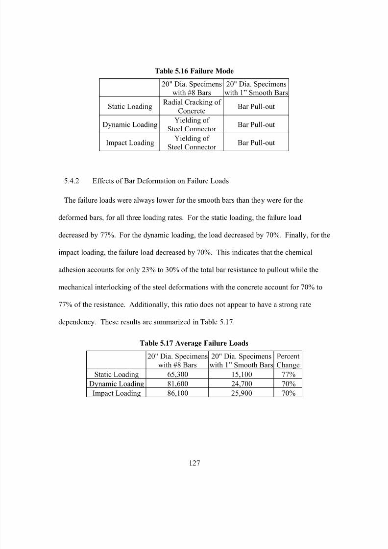
7/28/2019 Weathersby Dis
http://slidepdf.com/reader/full/weathersby-dis 144/280
127
Table 5.16 Failure Mode
20" Dia. Specimens
with #8 Bars
20" Dia. Specimens
with 1” Smooth BarsStatic Loading
Radial Cracking of
ConcreteBar Pull-out
Dynamic LoadingYielding of
Steel Connector Bar Pull-out
Impact LoadingYielding of
Steel Connector Bar Pull-out
5.4.2 Effects of Bar Deformation on Failure Loads
The failure loads were always lower for the smooth bars than they were for the
deformed bars, for all three loading rates. For the static loading, the failure load
decreased by 77%. For the dynamic loading, the load decreased by 70%. Finally, for the
impact loading, the failure load decreased by 70%. This indicates that the chemical
adhesion accounts for only 23% to 30% of the total bar resistance to pullout while the
mechanical interlocking of the steel deformations with the concrete account for 70% to
77% of the resistance. Additionally, this ratio does not appear to have a strong rate
dependency. These results are summarized in Table 5.17.
Table 5.17 Average Failure Loads
20" Dia. Specimens
with #8 Bars
20" Dia. Specimens
with 1” Smooth Bars
Percent
Change
Static Loading 65,300 15,100 77%
Dynamic Loading 81,600 24,700 70%Impact Loading 86,100 25,900 70%
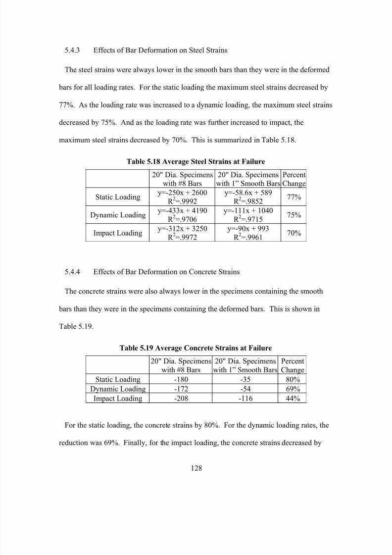
7/28/2019 Weathersby Dis
http://slidepdf.com/reader/full/weathersby-dis 145/280
128
5.4.3 Effects of Bar Deformation on Steel Strains
The steel strains were always lower in the smooth bars than they were in the deformed
bars for all loading rates. For the static loading the maximum steel strains decreased by
77%. As the loading rate was increased to a dynamic loading, the maximum steel strains
decreased by 75%. And as the loading rate was further increased to impact, the
maximum steel strains decreased by 70%. This is summarized in Table 5.18.
Table 5.18 Average Steel Strains at Failure
20" Dia. Specimenswith #8 Bars
20" Dia. Specimenswith 1” Smooth Bars
PercentChange
Static Loading y=-250x + 2600R
2=.9992
y=-58.6x + 589R
2=.9852
77%
Dynamic Loadingy=-433x + 4190
R 2=.9706
y=-111x + 1040
R 2=.9715
75%
Impact Loadingy=-312x + 3250
R 2=.9972
y=-90x + 993
R 2=.9961
70%
5.4.4 Effects of Bar Deformation on Concrete Strains
The concrete strains were also always lower in the specimens containing the smooth
bars than they were in the specimens containing the deformed bars. This is shown in
Table 5.19.
Table 5.19 Average Concrete Strains at Failure
20" Dia. Specimens
with #8 Bars
20" Dia. Specimens
with 1” Smooth Bars
Percent
Change
Static Loading -180 -35 80%
Dynamic Loading -172 -54 69%Impact Loading -208 -116 44%
For the static loading, the concrete strains by 80%. For the dynamic loading rates, the
reduction was 69%. Finally, for the impact loading, the concrete strains decreased by
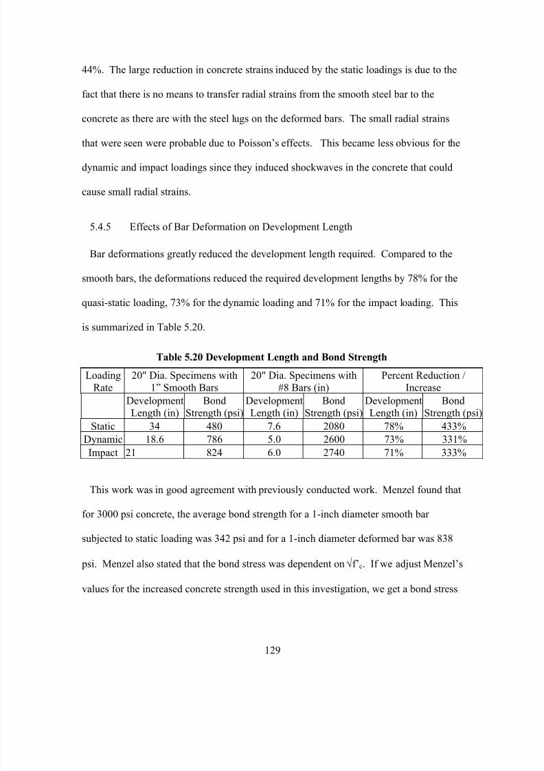
7/28/2019 Weathersby Dis
http://slidepdf.com/reader/full/weathersby-dis 146/280
129
44%. The large reduction in concrete strains induced by the static loadings is due to the
fact that there is no means to transfer radial strains from the smooth steel bar to the
concrete as there are with the steel lugs on the deformed bars. The small radial strains
that were seen were probable due to Poisson’s effects. This became less obvious for the
dynamic and impact loadings since they induced shockwaves in the concrete that could
cause small radial strains.
5.4.5 Effects of Bar Deformation on Development Length
Bar deformations greatly reduced the development length required. Compared to the
smooth bars, the deformations reduced the required development lengths by 78% for the
quasi-static loading, 73% for the dynamic loading and 71% for the impact loading. This
is summarized in Table 5.20.
Table 5.20 Development Length and Bond Strength
Loading
Rate
20" Dia. Specimens with
1” Smooth Bars
20" Dia. Specimens with
#8 Bars (in)
Percent Reduction /
Increase
DevelopmentLength (in) BondStrength (psi) DevelopmentLength (in) BondStrength (psi) DevelopmentLength (in) BondStrength (psi)
Static 34 480 7.6 2080 78% 433%
Dynamic 18.6 786 5.0 2600 73% 331%
Impact 21 824 6.0 2740 71% 333%
This work was in good agreement with previously conducted work. Menzel found that
for 3000 psi concrete, the average bond strength for a 1-inch diameter smooth bar
subjected to static loading was 342 psi and for a 1-inch diameter deformed bar was 838
psi. Menzel also stated that the bond stress was dependent on √f’c. If we adjust Menzel’s
values for the increased concrete strength used in this investigation, we get a bond stress

7/28/2019 Weathersby Dis
http://slidepdf.com/reader/full/weathersby-dis 147/280
130
of 483 psi for the smooth bar and 1200 psi for the deformed bar. This compares well
with 480 psi for the smooth bar and 1310 psi for the deformed bar obtained for static
loading in this investigation and presented in Table 5.20.
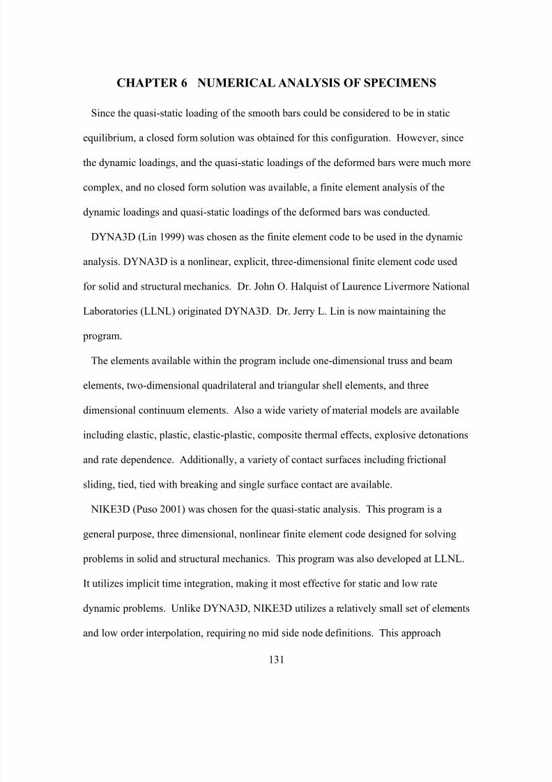
7/28/2019 Weathersby Dis
http://slidepdf.com/reader/full/weathersby-dis 148/280
131
CHAPTER 6 NUMERICAL ANALYSIS OF SPECIMENS
Since the quasi-static loading of the smooth bars could be considered to be in static
equilibrium, a closed form solution was obtained for this configuration. However, since
the dynamic loadings, and the quasi-static loadings of the deformed bars were much more
complex, and no closed form solution was available, a finite element analysis of the
dynamic loadings and quasi-static loadings of the deformed bars was conducted.
DYNA3D (Lin 1999) was chosen as the finite element code to be used in the dynamic
analysis. DYNA3D is a nonlinear, explicit, three-dimensional finite element code used
for solid and structural mechanics. Dr. John O. Halquist of Laurence Livermore National
Laboratories (LLNL) originated DYNA3D. Dr. Jerry L. Lin is now maintaining the
program.
The elements available within the program include one-dimensional truss and beam
elements, two-dimensional quadrilateral and triangular shell elements, and three
dimensional continuum elements. Also a wide variety of material models are available
including elastic, plastic, elastic-plastic, composite thermal effects, explosive detonations
and rate dependence. Additionally, a variety of contact surfaces including frictional
sliding, tied, tied with breaking and single surface contact are available.
NIKE3D (Puso 2001) was chosen for the quasi-static analysis. This program is a
general purpose, three dimensional, nonlinear finite element code designed for solving
problems in solid and structural mechanics. This program was also developed at LLNL.
It utilizes implicit time integration, making it most effective for static and low rate
dynamic problems. Unlike DYNA3D, NIKE3D utilizes a relatively small set of elements
and low order interpolation, requiring no mid side node definitions. This approach
7/28/2019 Weathersby Dis
http://slidepdf.com/reader/full/weathersby-dis 149/280
132
appears to be robust enough for non-linear quasi-static loadings while greatly reducing
the computing resources required for the analysis.
The elements available within NIKE3D include solid, beam and shell. The program
includes 22 material models including elastic, elastic-plastic, thermo elastic-plastic, and
thermo elastic creep. As with the element selection, the slide lines available in NIKE3D
are more limited then those in DYNA3D. These include tied, sliding only, sliding with
gaps and friction, single surface and auto contact.
The program INGRID (Christon 1992) that was also developed at LLNL was used as
the pre-processor for DYNA3D and NIKE3D. INGRID is a generalized 3-D finite
element mesh generator used for modeling non-linear systems. It provides the capability
to generate complex geometric models using beam, shell, and hexahedral elements.
Additionally, boundary conditions, initial conditions, material properties and contact
surfaces can be specified.
Finally, post-processing was accomplished using the LLNL program GRIZ (Speck
1996). GRIZ is a general-purpose post-processor application supporting interactive
visualization of finite element analysis results on unstructured grids. In addition to basic
state variable display, GRIZ provides 3-D visualization techniques such as isocontours,
isosurfaces, cutting planes, vector field display and partial tracing.
All four of these programs are part of a set of public domain codes developed in the
Methods Development Group at LLNL.
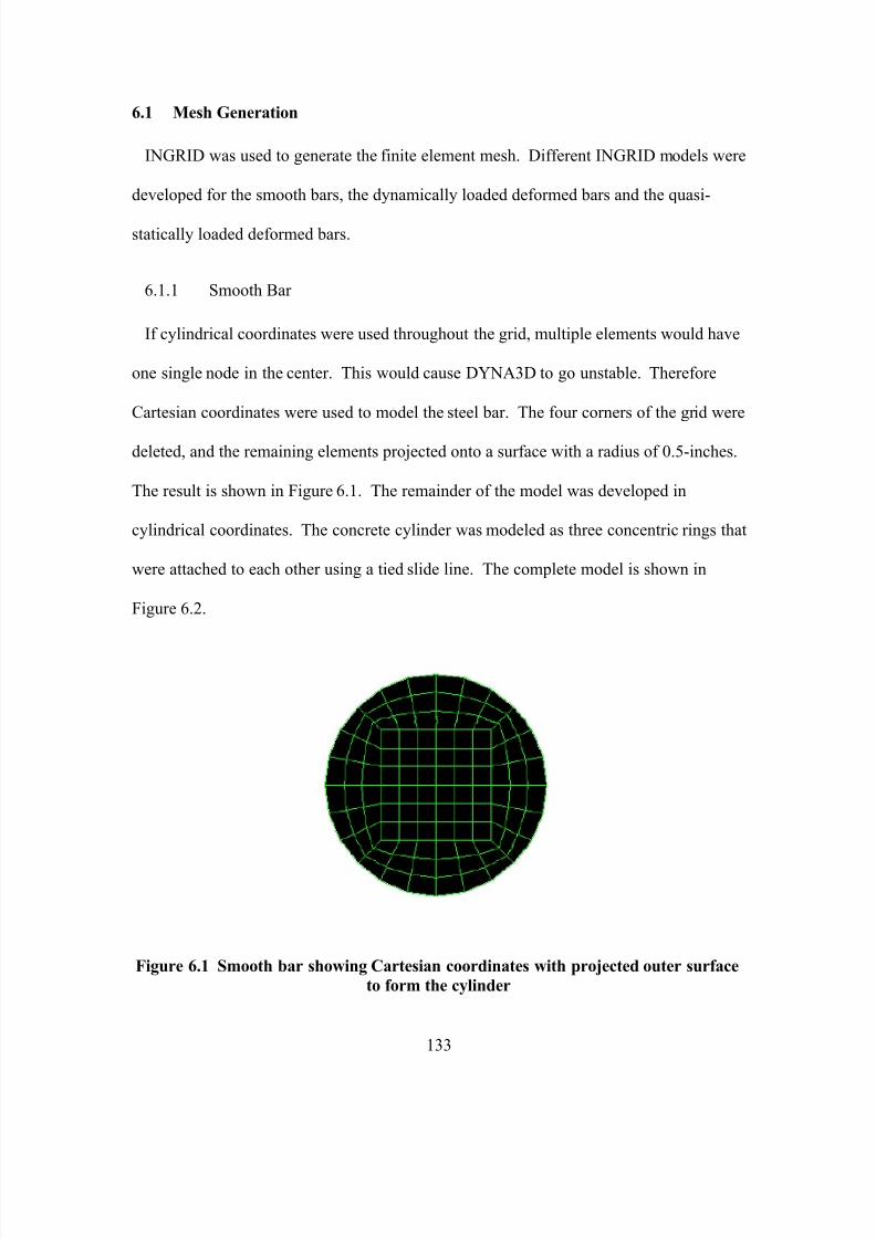
7/28/2019 Weathersby Dis
http://slidepdf.com/reader/full/weathersby-dis 150/280
133
6.1 Mesh Generation
INGRID was used to generate the finite element mesh. Different INGRID models were
developed for the smooth bars, the dynamically loaded deformed bars and the quasi-
statically loaded deformed bars.
6.1.1 Smooth Bar
If cylindrical coordinates were used throughout the grid, multiple elements would have
one single node in the center. This would cause DYNA3D to go unstable. Therefore
Cartesian coordinates were used to model the steel bar. The four corners of the grid were
deleted, and the remaining elements projected onto a surface with a radius of 0.5-inches.
The result is shown in Figure 6.1. The remainder of the model was developed in
cylindrical coordinates. The concrete cylinder was modeled as three concentric rings that
were attached to each other using a tied slide line. The complete model is shown in
Figure 6.2.
Figure 6.1 Smooth bar showing Cartesian coordinates with projected outer surface
to form the cylinder
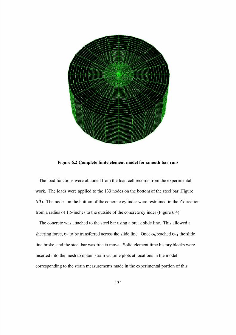
7/28/2019 Weathersby Dis
http://slidepdf.com/reader/full/weathersby-dis 151/280
134
Figure 6.2 Complete finite element model for smooth bar runs
The load functions were obtained from the load cell records from the experimental
work. The loads were applied to the 133 nodes on the bottom of the steel bar (Figure
6.3). The nodes on the bottom of the concrete cylinder were restrained in the Z direction
from a radius of 1.5-inches to the outside of the concrete cylinder (Figure 6.4).
The concrete was attached to the steel bar using a break slide line. This allowed a
sheering force, σS to be transferred across the slide line. Once σS reached σST the slide
line broke, and the steel bar was free to move. Solid element time history blocks were
inserted into the mesh to obtain strain vs. time plots at locations in the model
corresponding to the strain measurements made in the experimental portion of this
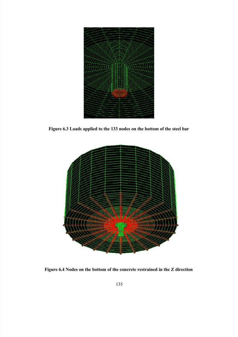
7/28/2019 Weathersby Dis
http://slidepdf.com/reader/full/weathersby-dis 152/280
135
Figure 6.3 Loads applied to the 133 nodes on the bottom of the steel bar
Figure 6.4 Nodes on the bottom of the concrete restrained in the Z direction
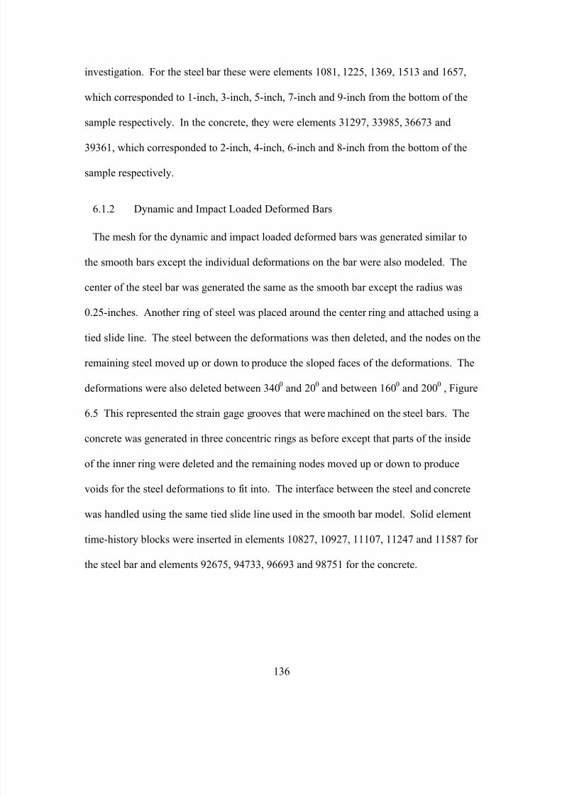
7/28/2019 Weathersby Dis
http://slidepdf.com/reader/full/weathersby-dis 153/280
136
investigation. For the steel bar these were elements 1081, 1225, 1369, 1513 and 1657,
which corresponded to 1-inch, 3-inch, 5-inch, 7-inch and 9-inch from the bottom of the
sample respectively. In the concrete, they were elements 31297, 33985, 36673 and
39361, which corresponded to 2-inch, 4-inch, 6-inch and 8-inch from the bottom of the
sample respectively.
6.1.2 Dynamic and Impact Loaded Deformed Bars
The mesh for the dynamic and impact loaded deformed bars was generated similar to
the smooth bars except the individual deformations on the bar were also modeled. The
center of the steel bar was generated the same as the smooth bar except the radius was
0.25-inches. Another ring of steel was placed around the center ring and attached using a
tied slide line. The steel between the deformations was then deleted, and the nodes on the
remaining steel moved up or down to produce the sloped faces of the deformations. The
deformations were also deleted between 3400
and 200
and between 1600
and 2000
, Figure
6.5 This represented the strain gage grooves that were machined on the steel bars. The
concrete was generated in three concentric rings as before except that parts of the inside
of the inner ring were deleted and the remaining nodes moved up or down to produce
voids for the steel deformations to fit into. The interface between the steel and concrete
was handled using the same tied slide line used in the smooth bar model. Solid element
time-history blocks were inserted in elements 10827, 10927, 11107, 11247 and 11587 for
the steel bar and elements 92675, 94733, 96693 and 98751 for the concrete.
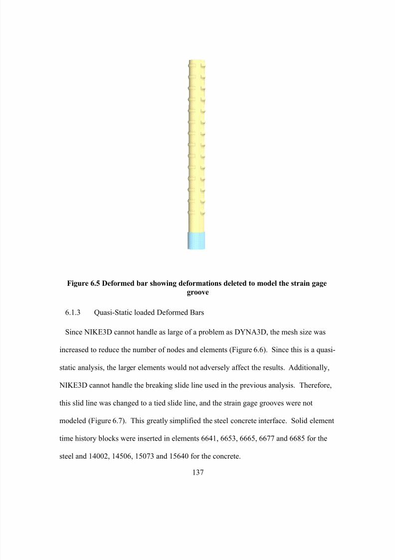
7/28/2019 Weathersby Dis
http://slidepdf.com/reader/full/weathersby-dis 154/280
137
Figure 6.5 Deformed bar showing deformations deleted to model the strain gage
groove
6.1.3 Quasi-Static loaded Deformed Bars
Since NIKE3D cannot handle as large of a problem as DYNA3D, the mesh size was
increased to reduce the number of nodes and elements (Figure 6.6). Since this is a quasi-
static analysis, the larger elements would not adversely affect the results. Additionally,
NIKE3D cannot handle the breaking slide line used in the previous analysis. Therefore,
this slid line was changed to a tied slide line, and the strain gage grooves were not
modeled (Figure 6.7). This greatly simplified the steel concrete interface. Solid element
time history blocks were inserted in elements 6641, 6653, 6665, 6677 and 6685 for the
steel and 14002, 14506, 15073 and 15640 for the concrete.
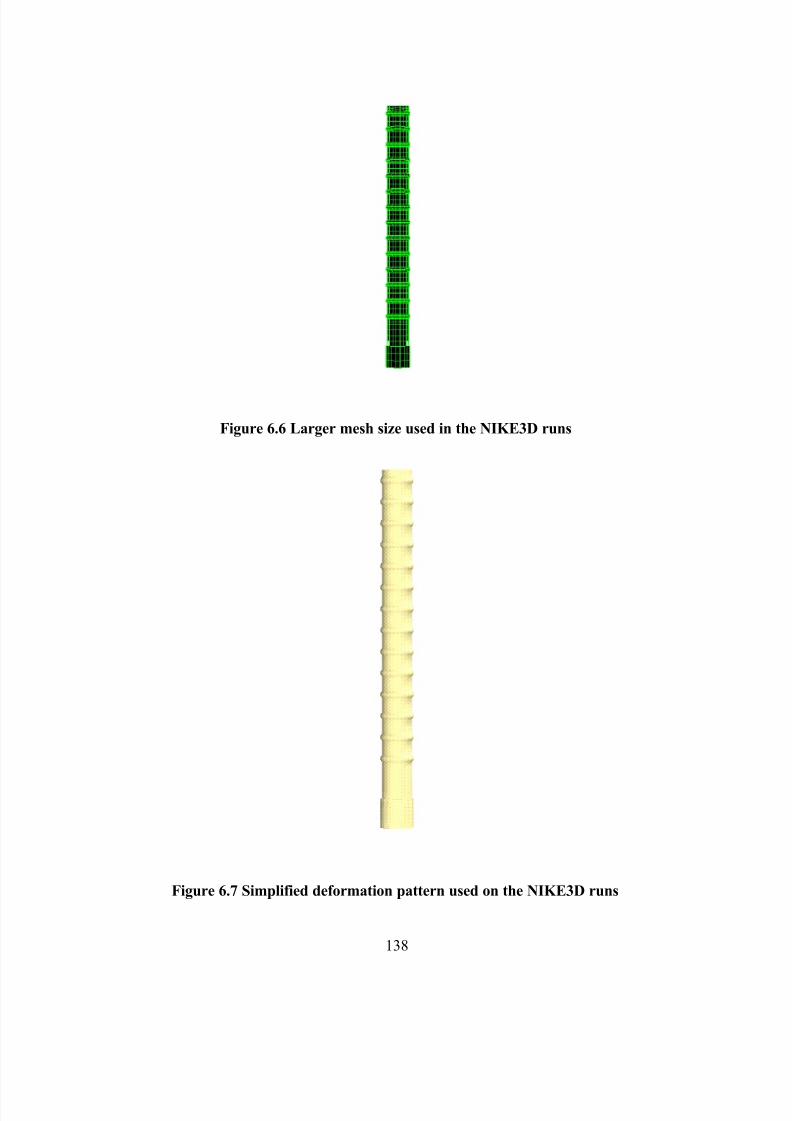
7/28/2019 Weathersby Dis
http://slidepdf.com/reader/full/weathersby-dis 155/280
138
Figure 6.6 Larger mesh size used in the NIKE3D runs
Figure 6.7 Simplified deformation pattern used on the NIKE3D runs
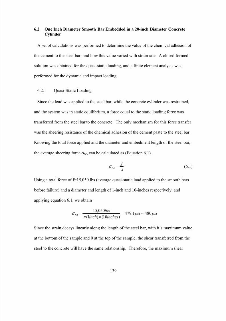
7/28/2019 Weathersby Dis
http://slidepdf.com/reader/full/weathersby-dis 156/280
139
6.2 One Inch Diameter Smooth Bar Embedded in a 20-inch Diameter Concrete
Cylinder
A set of calculations was performed to determine the value of the chemical adhesion of
the cement to the steel bar, and how this value varied with strain rate. A closed formed
solution was obtained for the quasi-static loading, and a finite element analysis was
performed for the dynamic and impact loading.
6.2.1 Quasi-Static Loading
Since the load was applied to the steel bar, while the concrete cylinder was restrained,
and the system was in static equilibrium, a force equal to the static loading force was
transferred from the steel bar to the concrete. The only mechanism for this force transfer
was the sheering resistance of the chemical adhesion of the cement paste to the steel bar.
Knowing the total force applied and the diameter and embedment length of the steel bar,
the average sheering force σSA can be calculated as (Equation 6.1).
A
f
SA=σ (6.1)
Using a total force of f=15,050 lbs (average quasi-static load applied to the smooth bars
before failure) and a diameter and length of 1-inch and 10-inches respectively, and
applying equation 6.1, we obtain
psi psiinchesinch
lbsSA 4801.479
)10()1(
050,15≈=
×=π
σ
Since the strain decays linearly along the length of the steel bar, with it’s maximum value
at the bottom of the sample and 0 at the top of the sample, the shear transferred from the
steel to the concrete will have the same relationship. Therefore, the maximum shear
7/28/2019 Weathersby Dis
http://slidepdf.com/reader/full/weathersby-dis 157/280
140
stress σST will occur at the bottom of the sample just prior to the bond failure, and will
decay linearly to 0 at the top of the sample. This leads to Equation 6.2.
SAST σ σ 2= (6.2)
Or for test 23 we obtain:
psi psiST 9604802 =×=σ
Since there are no means of transferring radial forces from the smooth steel bar to the
concrete, the radial strains will be very low. The small strains that were seen in the
experimental work (34.8 micro strains) were probably due to Poison’s effects
6.2.2 Dynamic Loading
A triangular loading function with a maximum value of 24,670 lbs and duration of 32
msec was used to simulate the average dynamic load applied to the smooth bars. An
initial estimate of σST was made, and the input deck for DYNA3D generated. DYNA3D
was then run on a Silicon Graphics workstation. Iterative runs were made until
calculated steel strains were in close agreement with those obtained from equation 4.8.
For these runs, σST was determined to be 2600 psi. As the run progressed, the strains in
the steel bar increased until t=27 msec., at which time the slide line broke, and the steel
bar was released. The maximum steel strain at each of the element dumps is shown in
Figure 6.8.
The concrete strains, although very small as would be expected, show a very unusual
response. The concrete first went into radial tension, and then into compression, then
back into tension before the slide line broke. The readings closest to the bottom of the
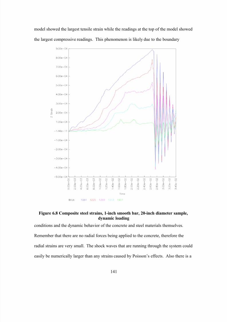
7/28/2019 Weathersby Dis
http://slidepdf.com/reader/full/weathersby-dis 158/280
141
model showed the largest tensile strain while the readings at the top of the model showed
the largest compressive readings. This phenomenon is likely due to the boundary
Figure 6.8 Composite steel strains, 1-inch smooth bar, 20-inch diameter sample,
dynamic loading
conditions and the dynamic behavior of the concrete and steel materials themselves.
Remember that there are no radial forces being applied to the concrete, therefore the
radial strains are very small. The shock waves that are running through the system could
easily be numerically larger than any strains caused by Poisson’s effects. Also there is a
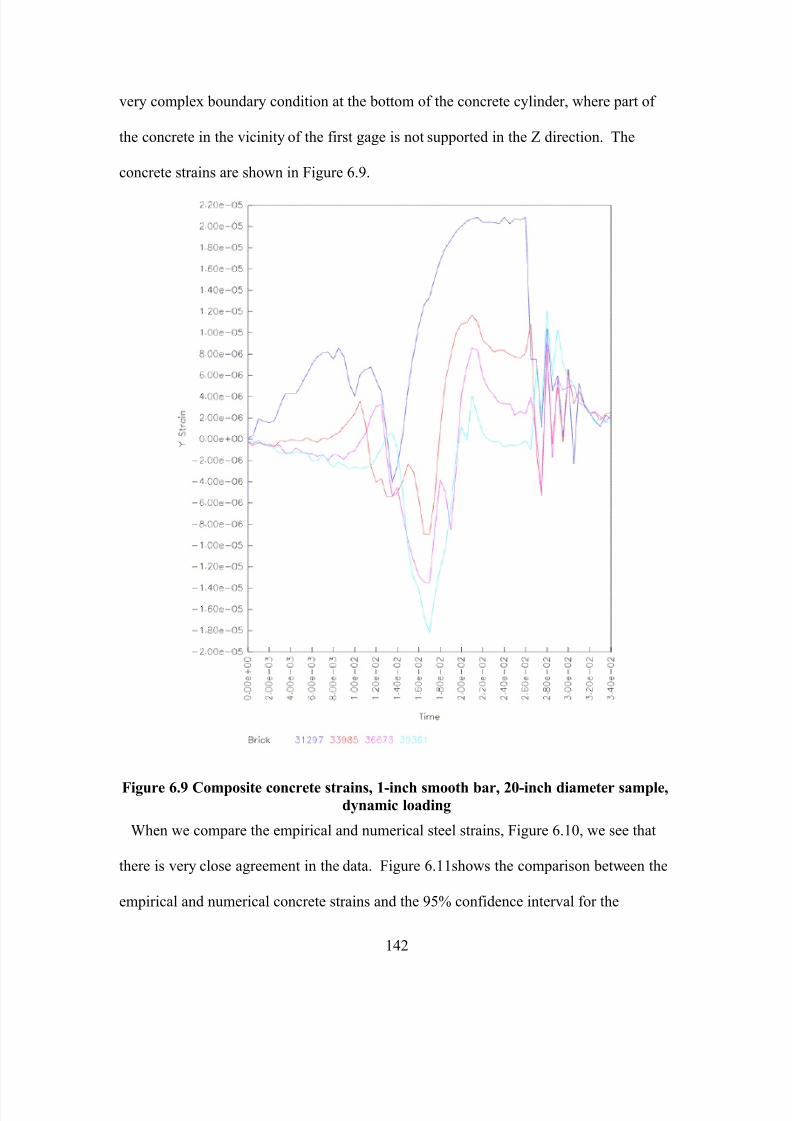
7/28/2019 Weathersby Dis
http://slidepdf.com/reader/full/weathersby-dis 159/280
142
very complex boundary condition at the bottom of the concrete cylinder, where part of
the concrete in the vicinity of the first gage is not supported in the Z direction. The
concrete strains are shown in Figure 6.9.
Figure 6.9 Composite concrete strains, 1-inch smooth bar, 20-inch diameter sample,dynamic loading
When we compare the empirical and numerical steel strains, Figure 6.10, we see that
there is very close agreement in the data. Figure 6.11shows the comparison between the
empirical and numerical concrete strains and the 95% confidence interval for the
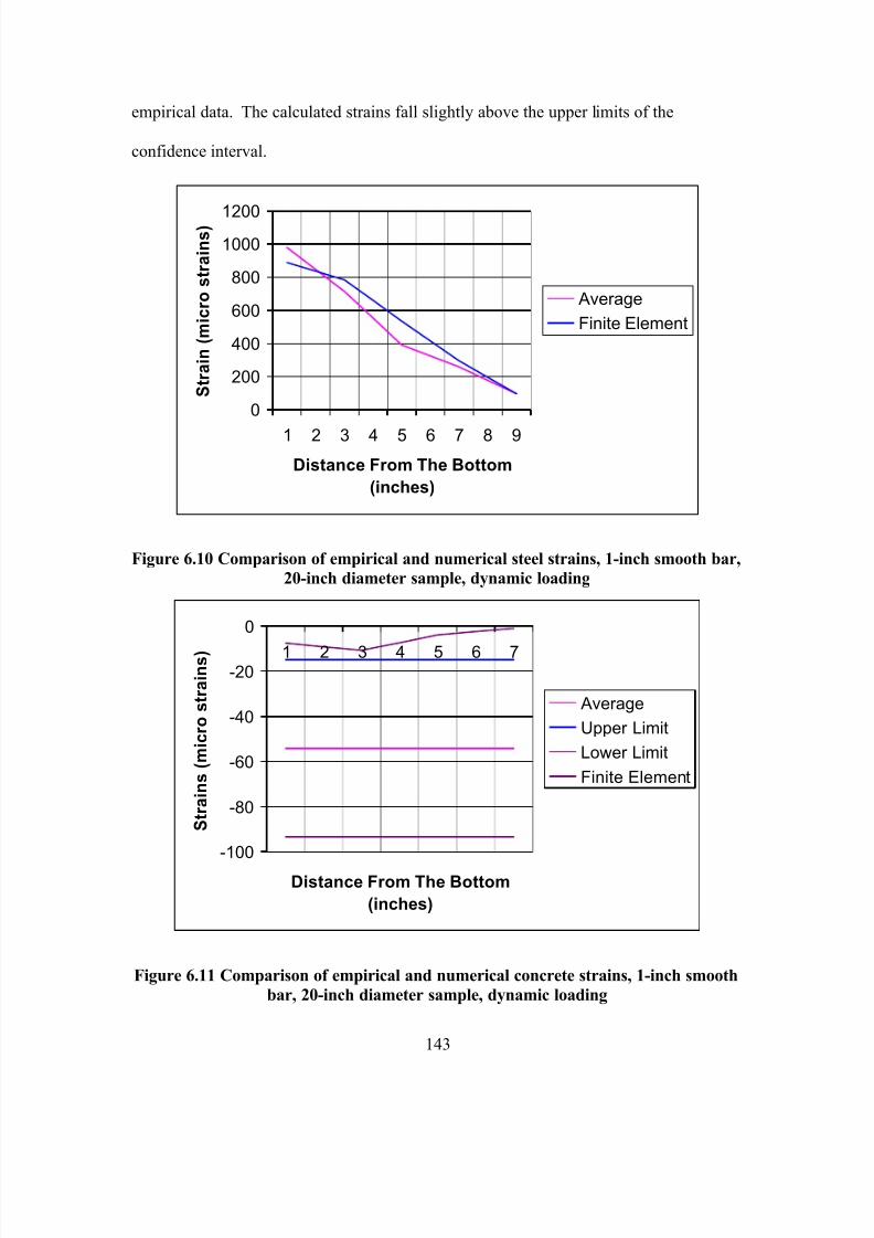
7/28/2019 Weathersby Dis
http://slidepdf.com/reader/full/weathersby-dis 160/280
143
empirical data. The calculated strains fall slightly above the upper limits of the
confidence interval.
0
200
400
600
800
10001200
1 2 3 4 5 6 7 8 9
Distance From The Bottom
(inches)
S t r a i n ( m i c r o s t r a i n s )
Average
Finite Element
Figure 6.10 Comparison of empirical and numerical steel strains, 1-inch smooth bar,
20-inch diameter sample, dynamic loading
-100
-80
-60
-40
-20
0
1 2 3 4 5 6 7
Distance From The Bottom
(inches)
S t r a i n s ( m i c r o s t r a i n s )
Average
Upper Limit
Lower Limit
Finite Element
Figure 6.11 Comparison of empirical and numerical concrete strains, 1-inch smooth
bar, 20-inch diameter sample, dynamic loading
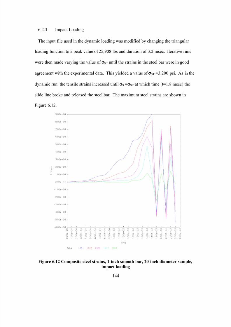
7/28/2019 Weathersby Dis
http://slidepdf.com/reader/full/weathersby-dis 161/280
144
6.2.3 Impact Loading
The input file used in the dynamic loading was modified by changing the triangular
loading function to a peak value of 25,908 lbs and duration of 3.2 msec. Iterative runs
were then made varying the value of σST until the strains in the steel bar were in good
agreement with the experimental data. This yielded a value of σST =3,200 psi. As in the
dynamic run, the tensile strains increased until σS =σST at which time (t=1.8 msec) the
slide line broke and released the steel bar. The maximum steel strains are shown in
Figure 6.12.
Figure 6.12 Composite steel strains, 1-inch smooth bar, 20-inch diameter sample,
impact loading
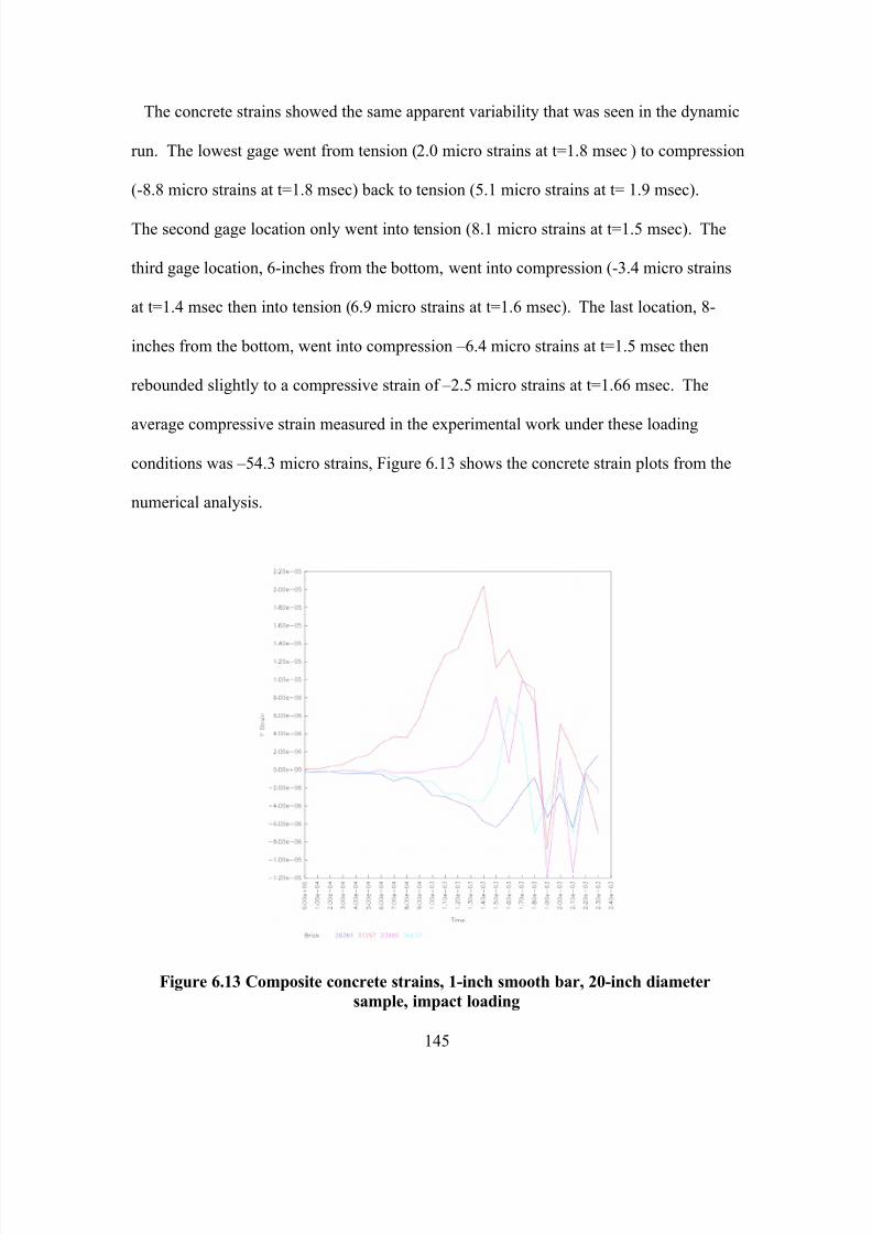
7/28/2019 Weathersby Dis
http://slidepdf.com/reader/full/weathersby-dis 162/280
145
The concrete strains showed the same apparent variability that was seen in the dynamic
run. The lowest gage went from tension (2.0 micro strains at t=1.8 msec ) to compression
(-8.8 micro strains at t=1.8 msec) back to tension (5.1 micro strains at t= 1.9 msec).
The second gage location only went into tension (8.1 micro strains at t=1.5 msec). The
third gage location, 6-inches from the bottom, went into compression (-3.4 micro strains
at t=1.4 msec then into tension (6.9 micro strains at t=1.6 msec). The last location, 8-
inches from the bottom, went into compression –6.4 micro strains at t=1.5 msec then
rebounded slightly to a compressive strain of –2.5 micro strains at t=1.66 msec. The
average compressive strain measured in the experimental work under these loading
conditions was –54.3 micro strains, Figure 6.13 shows the concrete strain plots from the
numerical analysis.
Figure 6.13 Composite concrete strains, 1-inch smooth bar, 20-inch diameter
sample, impact loading
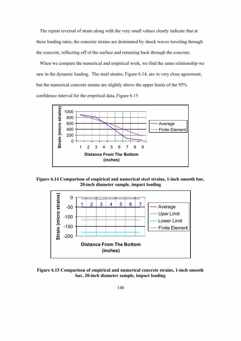
7/28/2019 Weathersby Dis
http://slidepdf.com/reader/full/weathersby-dis 163/280
146
The repeat reversal of strain along with the very small values clearly indicate that at
these loading rates, the concrete strains are dominated by shock waves traveling through
the concrete, reflecting off of the surface and returning back through the concrete.
When we compare the numerical and empirical work, we find the same relationship we
saw in the dynamic loading. The steel strains, Figure 6.14, are in very close agreement,
but the numerical concrete strains are slightly above the upper limits of the 95%
confidence interval for the empirical data, Figure 6.15
0
200
400
600800
1000
1 2 3 4 5 6 7 8 9
Distance From The Bottom
(inches)
S t r a i n ( m i c r o s t r a i n s )
Average
Finite Element
Figure 6.14 Comparison of empirical and numerical steel strains, 1-inch smooth bar,20-inch diameter sample, impact loading
-200
-150
-100
-50
0
1 2 3 4 5 6 7
Distance From The Bottom
(inches)
S
t r a i n ( m i c r o s t r a i n s )
Average
Uper Limit
Lower Limit
Finite Element
Figure 6.15 Comparison of empirical and numerical concrete strains, 1-inch smooth
bar, 20-inch diameter sample, impact loading
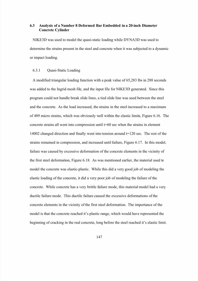
7/28/2019 Weathersby Dis
http://slidepdf.com/reader/full/weathersby-dis 164/280
147
6.3 Analysis of a Number 8 Deformed Bar Embedded in a 20-inch Diameter
Concrete Cylinder
NIKE3D was used to model the quasi-static loading while DYNA3D was used to
determine the strains present in the steel and concrete when it was subjected to a dynamic
or impact loading.
6.3.1 Quasi-Static Loading
A modified triangular loading function with a peak value of 65,283 lbs in 288 seconds
was added to the Ingrid mesh file, and the input file for NIKE3D generated. Since this
program could not handle break slide lines, a tied slide line was used between the steel
and the concrete. As the load increased, the strains in the steel increased to a maximum
of 489 micro strains, which was obviously well within the elastic limits, Figure 6.16. The
concrete strains all went into compression until t=60 sec when the strains in element
14002 changed direction and finally went into tension around t=120 sec. The rest of the
strains remained in compression, and increased until failure, Figure 6.17. In this model,
failure was caused by excessive deformation of the concrete elements in the vicinity of
the first steel deformation, Figure 6.18. As was mentioned earlier, the material used to
model the concrete was elastic-plastic. While this did a very good job of modeling the
elastic loading of the concrete, it did a very poor job of modeling the failure of the
concrete. While concrete has a very brittle failure mode, this material model had a very
ductile failure mode. This ductile failure caused the excessive deformations of the
concrete elements in the vicinity of the first steel deformation. The importance of the
model is that the concrete reached it’s plastic range, which would have represented the
beginning of cracking in the real concrete, long before the steel reached it’s elastic limit.
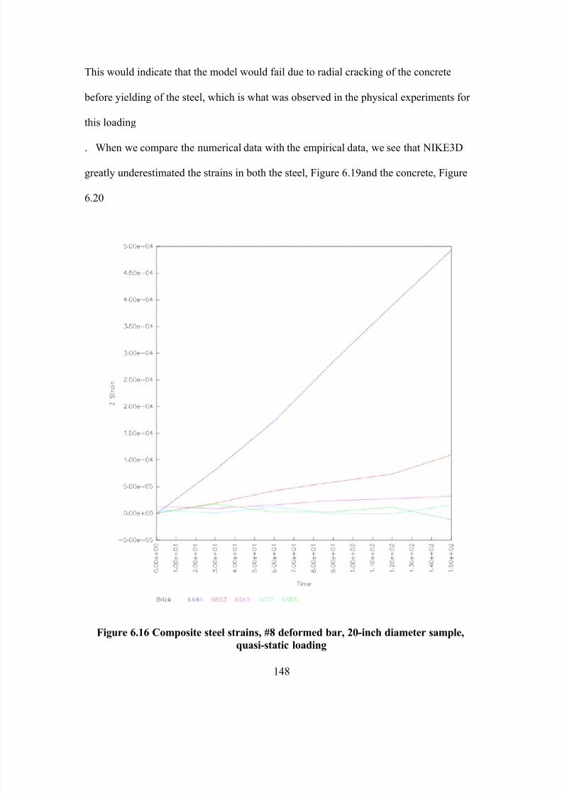
7/28/2019 Weathersby Dis
http://slidepdf.com/reader/full/weathersby-dis 165/280
148
This would indicate that the model would fail due to radial cracking of the concrete
before yielding of the steel, which is what was observed in the physical experiments for
this loading
. When we compare the numerical data with the empirical data, we see that NIKE3D
greatly underestimated the strains in both the steel, Figure 6.19and the concrete, Figure
6.20
Figure 6.16 Composite steel strains, #8 deformed bar, 20-inch diameter sample,
quasi-static loading
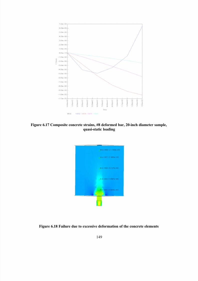
7/28/2019 Weathersby Dis
http://slidepdf.com/reader/full/weathersby-dis 166/280
149
Figure 6.17 Composite concrete strains, #8 deformed bar, 20-inch diameter sample,
quasi-static loading
Figure 6.18 Failure due to excessive deformation of the concrete elements
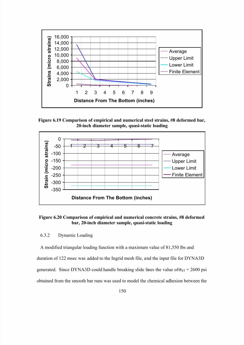
7/28/2019 Weathersby Dis
http://slidepdf.com/reader/full/weathersby-dis 167/280
150
0
2,000
4,000
6,0008,000
10,000
12,000
14,000
16,000
1 2 3 4 5 6 7 8 9
Distance From The Bottom (inches)
S t r a i n s ( m i c
r o s t r a i n s )
Average
Upper LimitLower Limit
Finite Element
Figure 6.19 Comparison of empirical and numerical steel strains, #8 deformed bar,20-inch diameter sample, quasi-static loading
-350
-300
-250
-200
-150
-100
-50
0
1 2 3 4 5 6 7
Distance From The Bottom (inches)
S t r a
i n ( m i c r o s t r a i n s )
Average
Upper Limit
Lower Limit
Finite Element
Figure 6.20 Comparison of empirical and numerical concrete strains, #8 deformed
bar, 20-inch diameter sample, quasi-static loading
6.3.2 Dynamic Loading
A modified triangular loading function with a maximum value of 81,550 lbs and
duration of 122 msec was added to the Ingrid mesh file, and the input file for DYNA3D
generated. Since DYNA3D could handle breaking slide lines the value of σST = 2600 psi
obtained from the smooth bar runs was used to model the chemical adhesion between the
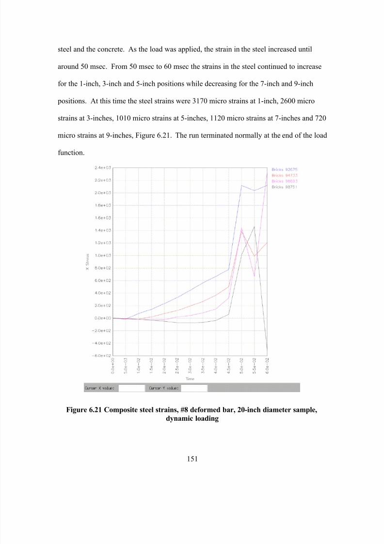
7/28/2019 Weathersby Dis
http://slidepdf.com/reader/full/weathersby-dis 168/280
151
steel and the concrete. As the load was applied, the strain in the steel increased until
around 50 msec. From 50 msec to 60 msec the strains in the steel continued to increase
for the 1-inch, 3-inch and 5-inch positions while decreasing for the 7-inch and 9-inch
positions. At this time the steel strains were 3170 micro strains at 1-inch, 2600 micro
strains at 3-inches, 1010 micro strains at 5-inches, 1120 micro strains at 7-inches and 720
micro strains at 9-inches, Figure 6.21. The run terminated normally at the end of the load
function.
Figure 6.21 Composite steel strains, #8 deformed bar, 20-inch diameter sample,
dynamic loading
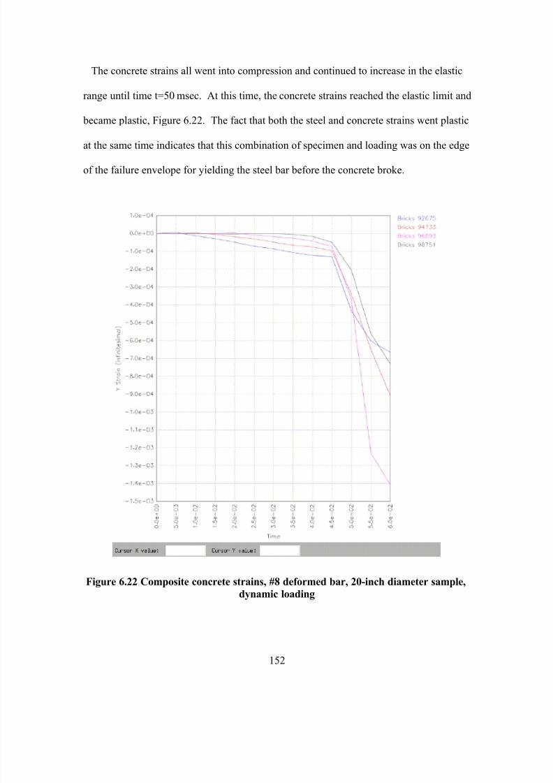
7/28/2019 Weathersby Dis
http://slidepdf.com/reader/full/weathersby-dis 169/280
152
The concrete strains all went into compression and continued to increase in the elastic
range until time t=50 msec. At this time, the concrete strains reached the elastic limit and
became plastic, Figure 6.22. The fact that both the steel and concrete strains went plastic
at the same time indicates that this combination of specimen and loading was on the edge
of the failure envelope for yielding the steel bar before the concrete broke.
Figure 6.22 Composite concrete strains, #8 deformed bar, 20-inch diameter sample,
dynamic loading
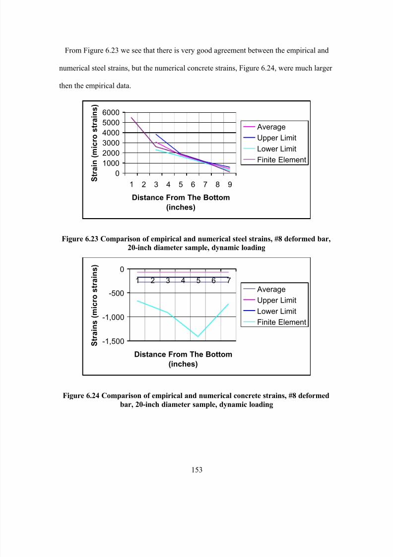
7/28/2019 Weathersby Dis
http://slidepdf.com/reader/full/weathersby-dis 170/280
153
From Figure 6.23 we see that there is very good agreement between the empirical and
numerical steel strains, but the numerical concrete strains, Figure 6.24, were much larger
then the empirical data.
0
1000
2000
3000
4000
5000
6000
1 2 3 4 5 6 7 8 9
Distance From The Bottom
(inches)
S t r a i n ( m i c r o s t r a i n s )
Average
Upper Limit
Lower Limit
Finite Element
Figure 6.23 Comparison of empirical and numerical steel strains, #8 deformed bar,
20-inch diameter sample, dynamic loading
-1,500
-1,000
-500
0
1 2 3 4 5 6 7
Distance From The Bottom
(inches)
S t r a i n s ( m i c r o s t r a i n s )
AverageUpper Limit
Lower Limit
Finite Element
Figure 6.24 Comparison of empirical and numerical concrete strains, #8 deformed
bar, 20-inch diameter sample, dynamic loading
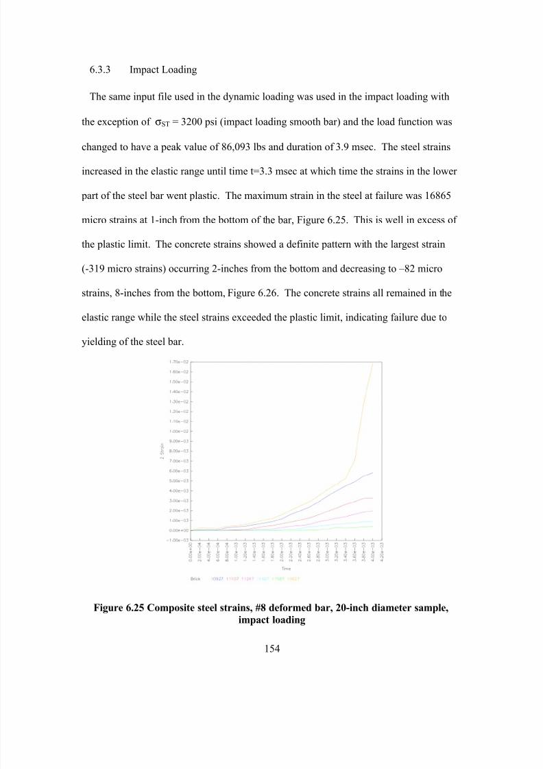
7/28/2019 Weathersby Dis
http://slidepdf.com/reader/full/weathersby-dis 171/280
154
6.3.3 Impact Loading
The same input file used in the dynamic loading was used in the impact loading with
the exception of σST = 3200 psi (impact loading smooth bar) and the load function was
changed to have a peak value of 86,093 lbs and duration of 3.9 msec. The steel strains
increased in the elastic range until time t=3.3 msec at which time the strains in the lower
part of the steel bar went plastic. The maximum strain in the steel at failure was 16865
micro strains at 1-inch from the bottom of the bar, Figure 6.25. This is well in excess of
the plastic limit. The concrete strains showed a definite pattern with the largest strain
(-319 micro strains) occurring 2-inches from the bottom and decreasing to –82 micro
strains, 8-inches from the bottom, Figure 6.26. The concrete strains all remained in the
elastic range while the steel strains exceeded the plastic limit, indicating failure due to
yielding of the steel bar.
Figure 6.25 Composite steel strains, #8 deformed bar, 20-inch diameter sample,
impact loading
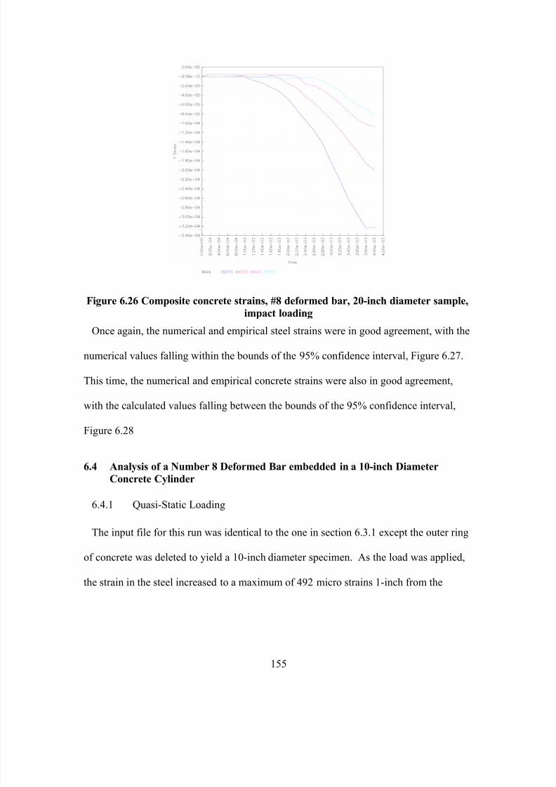
7/28/2019 Weathersby Dis
http://slidepdf.com/reader/full/weathersby-dis 172/280
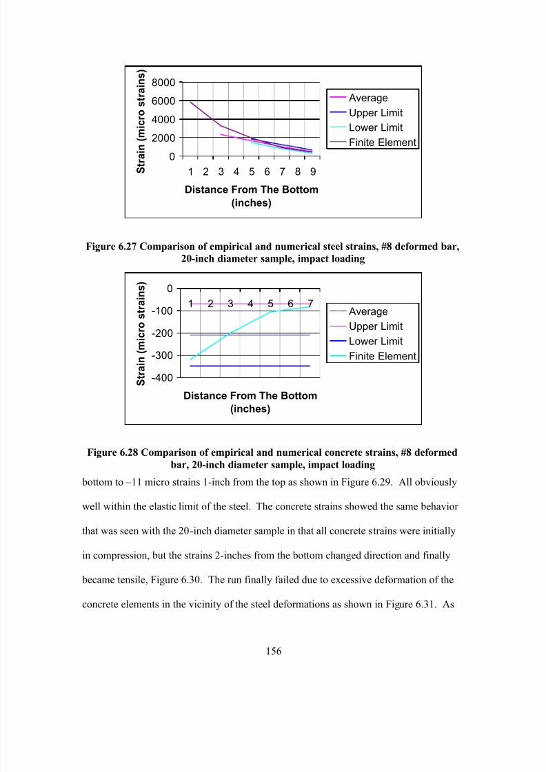
7/28/2019 Weathersby Dis
http://slidepdf.com/reader/full/weathersby-dis 173/280
156
0
2000
4000
6000
8000
1 2 3 4 5 6 7 8 9
Distance From The Bottom
(inches)
S t r a i n ( m
i c r o s t r a i n s )
Average
Upper Limit
Lower Limit
Finite Element
Figure 6.27 Comparison of empirical and numerical steel strains, #8 deformed bar,
20-inch diameter sample, impact loading
-400
-300
-200
-100
0
1 2 3 4 5 6 7
Distance From The Bottom
(inches)
S t r a i n ( m i c r o s t r a i n s )
Average
Upper Limit
Lower Limit
Finite Element
Figure 6.28 Comparison of empirical and numerical concrete strains, #8 deformed
bar, 20-inch diameter sample, impact loading
bottom to –11 micro strains 1-inch from the top as shown in Figure 6.29. All obviously
well within the elastic limit of the steel. The concrete strains showed the same behavior
that was seen with the 20-inch diameter sample in that all concrete strains were initially
in compression, but the strains 2-inches from the bottom changed direction and finally
became tensile, Figure 6.30. The run finally failed due to excessive deformation of the
concrete elements in the vicinity of the steel deformations as shown in Figure 6.31. As
7/28/2019 Weathersby Dis
http://slidepdf.com/reader/full/weathersby-dis 174/280
157
was stated in section 6.3.1, this indicated that the concrete reached its plastic limit and
failed due to radial cracking of the concrete before yielding of the steel bar.
As with the quasi-static loading of the 20-inch diameter sample, NIKE3D
underestimated both the steel stresses (Figure 6.32) and the concrete stresses (Figure
6.33).
Figure 6.29 Composite steel strains, #8 deformed bar, 10-inch diameter sample,
quasi-static loading
7/28/2019 Weathersby Dis
http://slidepdf.com/reader/full/weathersby-dis 175/280
158
Figure 6.30 Composite concrete strains, #8 deformed bar, 10-inch diameter sample,
quasi-static loading
Figure 6.31 Failure due to excessive deformation of the concrete elements
7/28/2019 Weathersby Dis
http://slidepdf.com/reader/full/weathersby-dis 176/280
159
0
500
1,000
1,500
2,000
2,500
1 2 3 4 5 6 7 8 9
Distance From The Bottom
(inches)
S t r a i n ( m i c
r o s t r a i n s )
Average
Upper Limit
Lower Limit
Finite Element
Figure 6.32 Comparison of empirical and numerical steel strains, #8 deformed bar,10-inch diameter sample, quasi-static loading
-350
-300
-250
-200
-150
-100
-50
0
1 2 3 4 5 6 7
Distance From The Bottom
(inches)
S t r a
i n ( m i c r o s t r a i n s )
Average
Upper Limit
Lower Limit
Finite Element
Figure 6.33 Comparison of empirical and numerical concrete strains, #8 deformed
bar, 10-inch diameter sample, quasi-static loading
6.4.2 Dynamic Loading
This input file was the same as the one in Section 6.3.2 except that the outer ring of
concrete was removed to yield a 10-inch diameter model. The steel strains increased as
the load was applied until at time t=70 msec, the steel strains varied from a maximum of
7/28/2019 Weathersby Dis
http://slidepdf.com/reader/full/weathersby-dis 177/280
160
6480 micro strains at 1-inch from the bottom to 43 micro strains 1-inch from the top, as
shown in Figure 6.34. At approximately the same time, the concrete strains all went
plastic, Figure 6.35. The run finally failed at time t=80 msec due to excessive
deformation of the concrete elements. As with the 20-inch diameter specimen, this seems
to be an almost balanced failure with both the concrete and steel strains becoming plastic
at the same time.
Figure 6.34 Composite steel strains, #8 deformed bar, 10-inch diameter sample,
dynamic loading
When we compare the numerical and empirical data, we find that the numerical steel
strains are larger than the empirical strains at the bottom of the specimen, but come in
agreement at the top, Figure 6.36. The numerical concrete strains are larger than the
average empirical strains, but within the 95% confidence interval, Figure 6.37.
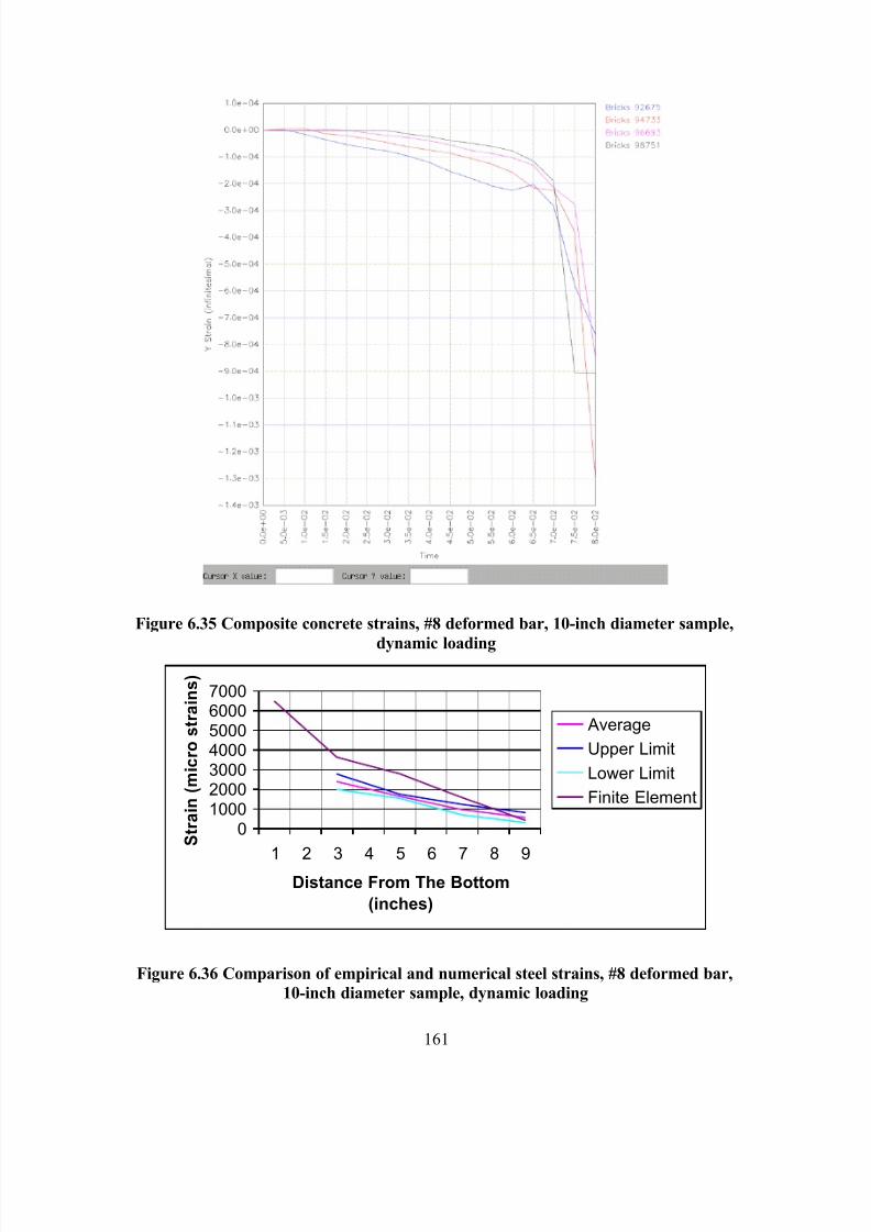
7/28/2019 Weathersby Dis
http://slidepdf.com/reader/full/weathersby-dis 178/280
161
Figure 6.35 Composite concrete strains, #8 deformed bar, 10-inch diameter sample,
dynamic loading
01000200030004000500060007000
1 2 3 4 5 6 7 8 9
Distance From The Bottom
(inches)
S t r a i n ( m i c r o s t r a i n s )
Average
Upper Limit
Lower Limit
Finite Element
Figure 6.36 Comparison of empirical and numerical steel strains, #8 deformed bar,
10-inch diameter sample, dynamic loading
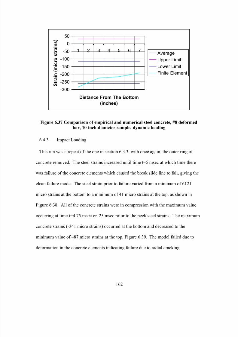
7/28/2019 Weathersby Dis
http://slidepdf.com/reader/full/weathersby-dis 179/280
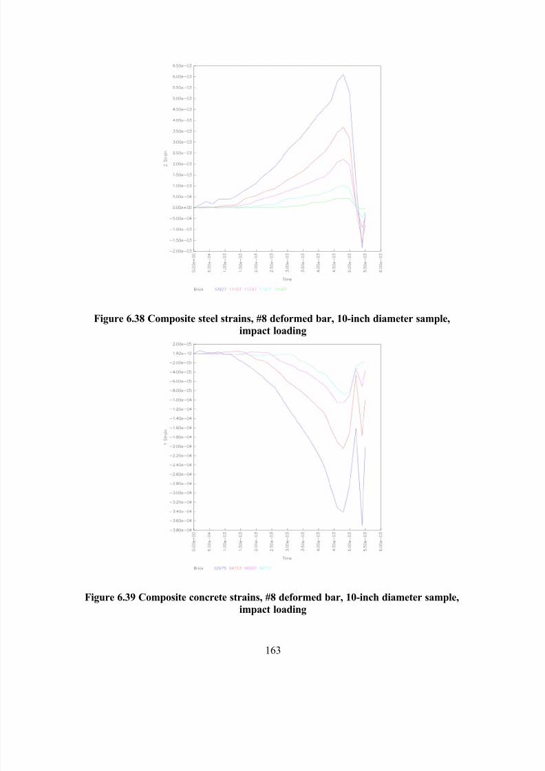
7/28/2019 Weathersby Dis
http://slidepdf.com/reader/full/weathersby-dis 180/280
163
Figure 6.38 Composite steel strains, #8 deformed bar, 10-inch diameter sample,
impact loading
Figure 6.39 Composite concrete strains, #8 deformed bar, 10-inch diameter sample,
impact loading
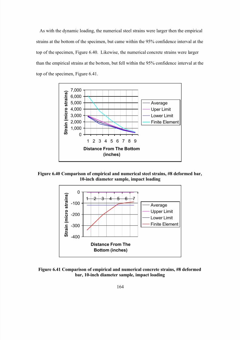
7/28/2019 Weathersby Dis
http://slidepdf.com/reader/full/weathersby-dis 181/280
164
As with the dynamic loading, the numerical steel strains were larger then the empirical
strains at the bottom of the specimen, but came within the 95% confidence interval at the
top of the specimen, Figure 6.40. Likewise, the numerical concrete strains were larger
than the empirical strains at the bottom, but fell within the 95% confidence interval at the
top of the specimen, Figure 6.41.
0
1,000
2,000
3,000
4,000
5,000
6,000
7,000
1 2 3 4 5 6 7 8 9
Distance From The Bottom
(inches)
S t r a i n ( m
i c r o s t r a i n s )
Average
Uper Limit
Lower Limit
Finite Element
Figure 6.40 Comparison of empirical and numerical steel strains, #8 deformed bar,
10-inch diameter sample, impact loading
-400
-300
-200
-100
0
1 2 3 4 5 6 7
Distance From The
Bottom (inches)
S t r a i n ( m i c r o s t r a i n s )
Average
Upper Limit
Lower Limit
Finite Element
Figure 6.41 Comparison of empirical and numerical concrete strains, #8 deformed
bar, 10-inch diameter sample, impact loading

7/28/2019 Weathersby Dis
http://slidepdf.com/reader/full/weathersby-dis 182/280
165
CHAPTER 7 SUMMARY, CONCLUSIONS AND
RECOMMENDATIONS
7.1 Summary
An experimental and analytical study was conducted to determine for static and
dynamic loading conditions; a) the chemical adhesion between the smooth steel bars and
concrete, b) the increase in pullout resistance of smooth and deformed bars, c) the
influence of concrete confinement and bar diameter on pullout resistance. Finite Element
Method of analysis was utilized to conduct the analytical study.
The experimental study involved the testing of 33 pullout specimens representing a
range of bar sizes, types and confinements. All the test specimens failed in one of three
modes; pullout of the steel bar, radial cracking of the concrete, and yielding of the steel
bar. Failure due to pullout of steel occurred only in test specimens with smooth bars, and
the failure mode was independent of the loading rate. The only resistance to the pullout
of the smooth bars was the static friction and chemical adhesion of the cement paste to
the steel bar, and the dynamic friction once this bond was broken. It was determined that
the strength of the chemical adhesion and static friction increased with increasing loading
rates. The combined static friction and chemical adhesion was 960psi for the quasi-static
loading, 2600psi for the dynamic loading and 3200 psi for the impact loading. The static
friction and chemical adhesion values obtained for the quasi-static loadings compared
well with the values estimated based on Menzel’s study, namely 900 psi. This difference
is due to the higher strength of the concrete (5,000 psi vs. 3,000 psi) used in this
investigation.
Failure due to radial cracking of concrete occurred in all of the 10-inch diameter
specimens, which had #8 deformed bars, and all 20-inch diameter specimens with #10
7/28/2019 Weathersby Dis
http://slidepdf.com/reader/full/weathersby-dis 183/280
166
deformed bars, regardless of the loading rates. It is pertinent to point out that the
deformations in the #8 rebars contributed to a 70%-77% increase in pullout strength as
compared to the smooth bars and this increase was independent of loading rate.
Failure due to yielding of steel occurred in all the 20-inch diameter specimens with #8
deformed bars with the exception of the specimens subjected to quasi-static loading
which failure due to radial cracking.
The total load applied before failure increased as the loading rate increased for all test
specimens. The impact failure load increased between 70% to 100% over the quasi-static
failure load. It is very important to note that as long as the failure mode did not change,
the maximum loads applied to the specimens nearly doubled as the loading rates were
increased fro quasi-static to impact loading. This doubling is in agreement with the
dynamic load factor of 2.0 used to increase the design strength of materials subject to
impact loading (Biggs 1964).
The steel strains increased as the loading rate went from quasi-static to dynamic, then
decreased as the loading rate went from dynamic to impact, due to the nature of the test
set up. As was stated in Chapter 5, this was slightly misleading, and the actual strains in
the bar were larger in the impact loading than in the dynamic loading. Even though there
were large variations in the concrete strains, they tended to increase as the loading rate
increased.
Increased concrete confinement increased the strength of the system for all loading
rates. This was especially true for specimens tested under quasi-static loadings that failed
due to radial cracking of the concrete. For this loading case, doubling the concrete
confinement increased the failure load by 58%. The increase was less (20%) for the
7/28/2019 Weathersby Dis
http://slidepdf.com/reader/full/weathersby-dis 184/280
167
dynamic and impact loadings, but this was partly due to the failure mode shifting from
concrete cracking to steel yielding.
Since both the concrete and steel materials are rate dependent and exhibit increased
strength with increased loading rate, it was not surprising that all the test specimens all
showed an increase in strength with an increase in loading rate. The average bond stress
for the quasi-static loaded deformed bars was 1,310 psi for the 10-inch diameter
specimens, 2,080 psi for the 20-inch diameter specimens containing the #8 deformed bars
and 1,820 psi for the specimens containing the #10 deformed bars. This was in
agreement with the findings of ACI committee 408 which found that the average bond
stress for deformed bars ranged from 1,500 psi to 3,000 psi, but was often less due to
reduced concrete cover. It is also in agreement with Menzel’s work that found the bond
stress for a #8 deformed bar to be 838 psi for 3000 psi concrete. Menzel also stated that
the bond stress was dependent on √f’c. If we adjust Menzel’s values for the increased
concrete strength, we get a bond stress of 1200 psi.
DYNA3D was very effective in modeling the behavior of the test specimens
subjected to the dynamic and impact loadings, particularly where the failure was
controlled by pullout or yielding of the steel bar. The analysis results showed very good
agreement with the experimental data. The material type 10 (Isotropic-Elastic-Plastic-
Hydrodynamic) used to model the concrete, did a very good job in the elastic range, but
was not as good in the plastic range. The breaking slide line was very successful at
modeling the chemical adhesion of the cement paste to the smooth steel bars.
NIKE3D was not very successful at modeling the quasi-static loading cases. The lack
of a breaking slide line and a suitable material model for the concrete (material type 3

7/28/2019 Weathersby Dis
http://slidepdf.com/reader/full/weathersby-dis 185/280
168
Elastic-Plastic) caused the computer runs to fail prematurely and greatly underestimate
the strains in both the steel and the concrete. However, both programs were able to
determine the failure modes that occurred for each specimen and loading combination.
By extending the liner regression for the steel strains, the embedment length required to
develop the full yield strength of the steel bars (2000 micro strains) can be calculated.
Generally, the development lengths for the quasi-static loading was less than half that
required by the ACI code. This would be expected since under normal circumstances,
confinement would be much less, and the codes must contain a safety factor. The
development length also decreased as the loading rate was increased to dynamic then
increased slightly for the impact loading. As has been pointed out before, this is slightly
misleading, and is a result of the test setup. Increased confinement resulted in a decrease
in the development length, where as increased bar diameter resulted in increased
development lengths. Bar deformations were paramount in reducing the development
length for all loading rates. The deformations reduced the development lengths by 71%
to 78%.
This study has led to a greater understanding of the behavior of steel reinforcement and
concrete subjected to dynamic and impact loadings. In particular the quantifying of the
chemical adhesion and the contribution of the steel deformations under dynamic and
impact loadings will allow researcher to develop more realistic models for predicting the
response and failure of reinforced concrete structures. Finally, these data could be used
to develop a concrete/steel reinforcement slide line capable of modeling the
concrete/reinforcement interaction under varying load conditions. This would allow

7/28/2019 Weathersby Dis
http://slidepdf.com/reader/full/weathersby-dis 186/280
169
designers the ability to do detailed models of concrete reinforcement systems without the
need to model each individual deformation on the reinforcement.
7.2 Conclusions
The study has led to the following conclusions:
• The bond stress due to static friction and chemical adhesion is 960 psi for quasi-
static loading, 2600 psi for dynamic loading and 3200 psi for impact loading for
the concrete and steel used in the test program. The values for quasi-static
loading compare well with results reported in earlier studies.
• The deformations on the steel bars account for 70% to 77% of the total resistance
to pullout regardless of loading rate.
• Increased concrete confinement increased the pullout resistance regardless of
loading rate. However, this increase in resistance dropped significantly with
increase in loading rate.
• As long as the mode of failure remained constant, the impact-loaded specimens
had nearly twice the pullout resistance of the quasi-statically loaded specimens.
• Bond stresses for both the smooth and deformed bars were in good agreement
with previous quasi-static work.
• The development length decreased as loading rates increased.
• Development length decreased as confinement increased.
• DYNA3D was capable of modeling the complex bond slip behavior between the
steel and concrete. The breaking slide line was very effective in modeling the
chemical adhesion of the cement paste to the smooth bars.
7/28/2019 Weathersby Dis
http://slidepdf.com/reader/full/weathersby-dis 187/280
170
7.3 Recommendations
This study has led to the following recommendations:
• Testing a larger number of specimens would yield a better statistical analysis of
the data.
• Measuring the circumferential concrete strains would probably yield better
results. Since the circumferential strain at any radius is constant, the
commercially available concrete embedment strain gages could be used. This
would have produced more consistent concrete strain data then the methods
used in this investigation.
• Another finite element program capable of handling the quasi-static loadings
could be identified, and these runs redone.
• The DYNA3D experimental material type 45 (DTRA Concrete/Geological
Material) could be modified to handle direct shear. This modified material
model might be able to handle the brittle failure of the concrete better.
7/28/2019 Weathersby Dis
http://slidepdf.com/reader/full/weathersby-dis 188/280
171
BIBLIOGRAPHY
Papados, P. P., “DYNA3D-LLNL: Material Fitting for the Concrete/Geological Model
16, Versions 11, 17, and 1.02,” Technical Report SL-97-_(in preparation), U.S. Army
Engineer Waterways Experiment Station, Vicksburg, MS 1997.
Prinaris, A. A., and Papados, P. P., “Reinforced Concrete Bond Modeling in ExplicitComputations Using DYNA3D-LLNL,” Technical Report SL-96-_(in preparation), U.S.
Army Engineer Waterways Experiment Station, Vicksburg, MS 1996.
Malvar, L. J., and Simons, D. “Concrete Material Modeling in Explicit Computations,”
Recent Advances in Computational Structural Dynamics and High-Performance
Computing, Workshop organized at the U.S. Army Engineer Waterways Experiment
Station, Vicksburg, MS 1996.
Papados, P. P., Baylot, J. T., and Hall, R. L., “Analysis of Large Test Structure Task DIPOLE East 51,” Proceedings of the “Closed Session” 7th International Symposium onthe Interaction of the Effects of Conventional Weapons with Structures, 1995, pp 131-
138.
Prinaris, A. A., Papados, P. P., Hall R. L., and Baylot, J. T., “Bond Behavior on One-
Way RC Slabs Under Dynamic Loadings,” Proceedings of the 65th Shock and Vibration
Symposium, Volume III, Shock and Vibration Information Analysis Center, Booz, Allen,and Hamilton, Inc., Arlington, VA, pp 93-102. Presented at the 65th Shock and
Vibration Symposium, San Diego, CA, 31 October - 3 November 1994.
Bentur, A., Mindess, S., and Banthia, N.P., “The Fracture of Reinforced Concrete Under Impact Loading,” Mindess, S., and Shah, S.P. (eds), Cement-Based Composites: Strain-
Rate Effects on Fracture, Vol. 64, 1986, pp 225-234.
Bentur, A., Mindess, S., and Banthia, N.P., “The Behavior of Concrete Under Impact
Loading: Experimental Procedures and Methods of Analysis,” Materiaux et
Constructions, Vol. 19, No. 113, 1986, pp 371-378.
Banthia, N.P., Mindess, S., Bentur, A., and Pigeon, M., “Impact Testing of Concrete
Using a Drop Weight Impact Machine,” Experimental Mechanics, Vol. 29, No. 2, 1988,
pp 63-69.
Goto, Y., “Crack Formed in Concrete Around Deformed Tension Bars,” American
Concrete Institute Journal, Proceedings, Vol. 68, No. 4, 1971, pp 244-251.
Tepfers, R., “Cracking of Concrete Cover Along Anchored Deformed Reinforcing Bars,”
Magazine of Concrete Research, Vol. 31, 1979, pp 3-12.
7/28/2019 Weathersby Dis
http://slidepdf.com/reader/full/weathersby-dis 189/280
172
Vervuurt, A., Schlangen, E., and Van Mier, J.G.M., “Analysis of Anchor Pull-Out in
Concrete,” Accepted for publication in Materials and Structures (RILEM), 1993.
Vervuurt, A., and Van Mier, J.G.M., “A Lattice Approach for Analyzing Steel-Concrete
Bond-Slip-Layer Fracture,” American Concrete Institute Special Publication SP-156
Interface Fracture and Bond, pp 85-106.
Yan, C., and Mindess, S., “Effect of Fibers on Bond Behavior Under Impact Loading,”
Mindess, S., and Skalny, J. (eds.), Fibre-Reinforced Cementitious Materials,” Materials
Research Society, Pittsburgh, PA, Vol. 211, 1991, pp 139-148.
Yan, C., and Mindess, S., “Bond Between Concrete and Steel Reinforcing Bars Under
Impact Loading,” Brandt, A.H., and Marshall, I.H. (eds.), Brittle Matrix Composites 3,Elsevier Applied Science, 1991, pp 184-192.
Yan, C., “Bond Between Reinforcing Bars and Concrete Under Impact Loading,” Ph.D.
Thesis, Department of Civil Engineering, University of British Columbia, 1992, p 369.
Vos, I.E., and Reinhardt, H.W., “Influence of Loading Rate on Bond Behavior of
Reinforcing Steel and Prestressing Strands,” Materiaux et Constructions, Vol. 15, No. 85,1982, pp 3-10.
Vos, I.E., “Influence of Loading Rate and Radial Pressure on Bond in ReinforcedConcrete. A Numerical and Experimental Approach,” Ph.D. Thesis, Delft University of
Technology, 1983, p 234.
Lin, J.I., “DYNA3D A Nonlinear, Implicit, Three-Dimensional Finite Element Code for
Solid and Structural Mechanics User’s Manual,” Technical Report UCRL-MA-105268,
Laurence Livermore National Laboratory, CA, 1999.
Puso, M.A., “NIKE3D A Nonlinear, Implicit, Three-Dimensional Finite Element Code
for Solid and Structural Mechanics User’s Manual,” Technical Report UCRL-MA-
105268, Laurence Livermore National Laboratory, CA, 2001.
Christon, M.A., and Dovey, D., “INGRID A 3-D Mesh generator for Modeling Nonlinear
Systems User’s Manual,” Technical Report UCRL-MA-105268, Laurence Livermore National Laboratory, CA, 1992.
Speck, D.E., and Dovey, D.J., “GRIZ Finite Element Analysis Results Visualization for Unstructured Grids User Manual,” Technical Report UCRL-MA-105268, Laurence
Livermore National Laboratory, CA, 1996.
Bakis, C.E., Uppuluri, V.S., Nanni, A. and Boothby, T.E. “Analysis of Bonding
Mechanisms of Smooth and Lugged RFP Rods Embedded in Concrete,” Composites
Science and Technology, Vol. 58, August 1998, pp1307-1319.
7/28/2019 Weathersby Dis
http://slidepdf.com/reader/full/weathersby-dis 190/280
173
Furguson, P.M. and Thompson, J.N., “Development Length of High Strength Reinforcing
Bars in Bond,” Journal of the American Concrete Institute, July, 1962, pp 887-921.
McDermott, J.F., “Effect of Steel Strength and of Reinforcement Ratio on the Mode of
Failure and Strain Energy Capacity of Reinforced Concrete Beams,” Report by ACICommittee 439, American Concrete Institute Journal, March 1969, pp 165-172.
Filippou, F.C. and Taucer, F.F., “Fibre Beam–Column Model for Non-Linear analysis of
R/C Frames: Part 1 Formulation,” Earthquake Engineering and Structural Dynamics, Vol.25, 1996, pp 711-725.
Menzel, C.A., “Some Factors Influencing Results of Pull-Out Bond Tests,” Journal of theAmerican Concrete Institute, Vol.35, June 1939, pp 516-543.
Mitchell, D. et.al., “State-of-the-Art Report on Bond Under Cyclic Loads,” Reported byACI Committee 408, ACI 408.2R-92, 1992, pp 1-31.
Ferguson, P.M., and Thompson, J.N., “Development Length for Large High Strength
Reinforcing Bars,” Journal of the American Concrete Institute, January 1965, pp 71-91.
Popov, E.P., “Mechanics of Materials,” Prentice-Hall, Inc. Englewood Cliffs, NewJersey, 1976, pp 275-336.
Biggs, J.M., “Introduction to Structural Dynamics,” McGraw-Hill Book Company, NewYork, 1964, pp 199-233.
7/28/2019 Weathersby Dis
http://slidepdf.com/reader/full/weathersby-dis 191/280
174
APPENDIX A: STRESS-STRAIN CURVES FOR STEEL AND
CONCRETE
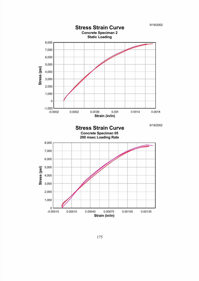
7/28/2019 Weathersby Dis
http://slidepdf.com/reader/full/weathersby-dis 192/280
175
9/19/2002
Strain (in/in)
S t r e s s ( p s i )
Stress Strain CurveConcrete Speciman 2
Static Loading
-0.0002 0.0002 0.0006 0.001 0.0014 0.0018-1,000
0
1,000
2,000
3,000
4,000
5,000
6,000
7,000
8,000
9/19/2002
Strain (in/in)
S t r e s s ( p s i )
Stress Strain CurveConcrete Speciman 05200 msec Loading Rate
-0.00015 0.00015 0.00045 0.00075 0.00105 0.001350
1,000
2,000
3,000
4,000
5,000
6,000
7,000
8,000
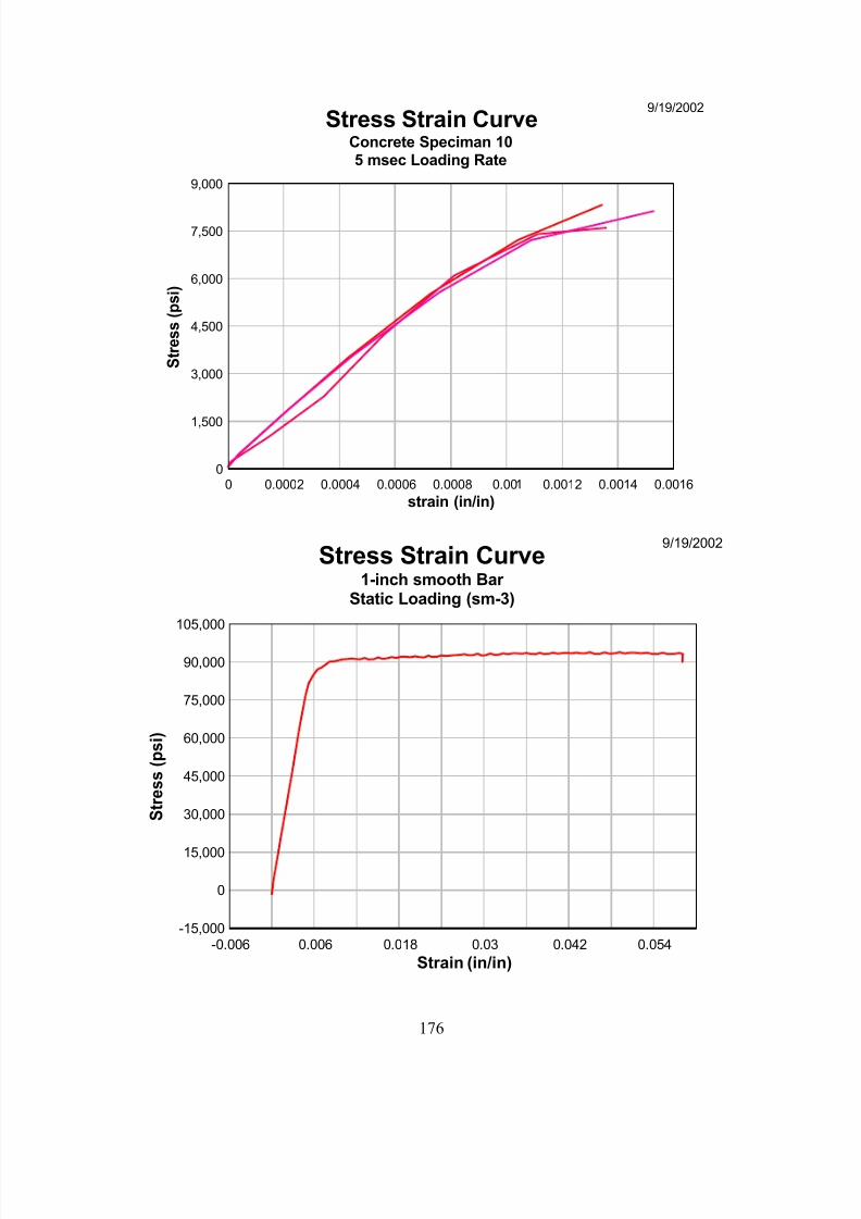
7/28/2019 Weathersby Dis
http://slidepdf.com/reader/full/weathersby-dis 193/280
176
9/19/2002
strain (in/in)
S t r e s s ( p s i )
Stress Strain CurveConcrete Speciman 105 msec Loading Rate
0 0.0002 0.0004 0.0006 0.0008 0.001 0.0012 0.0014 0.00160
1,500
3,000
4,500
6,000
7,500
9,000
9/19/2002
Strain (in/in)
S t r e s s ( p s i )
Stress Strain Curve1-inch smooth Bar
Static Loading (sm-3)
-0.006 0.006 0.018 0.03 0.042 0.054-15,000
0
15,000
30,000
45,000
60,000
75,000
90,000
105,000
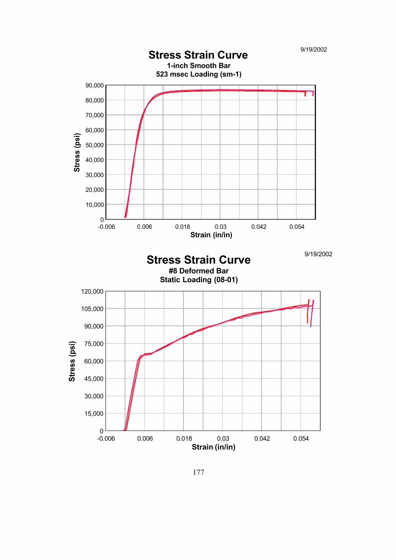
7/28/2019 Weathersby Dis
http://slidepdf.com/reader/full/weathersby-dis 194/280
177
9/19/2002
Strain (in/in)
S t r e s s ( p s i )
Stress Strain Curve1-inch Smooth Bar
523 msec Loading (sm-1)
-0.006 0.006 0.018 0.03 0.042 0.0540
10,000
20,000
30,000
40,000
50,000
60,000
70,000
80,000
90,000
9/19/2002
Strain (in/in)
S t r e s s ( p s i )
Stress Strain Curve#8 Deformed Bar
Static Loading (08-01)
-0.006 0.006 0.018 0.03 0.042 0.0540
15,000
30,000
45,000
60,000
75,000
90,000
105,000
120,000
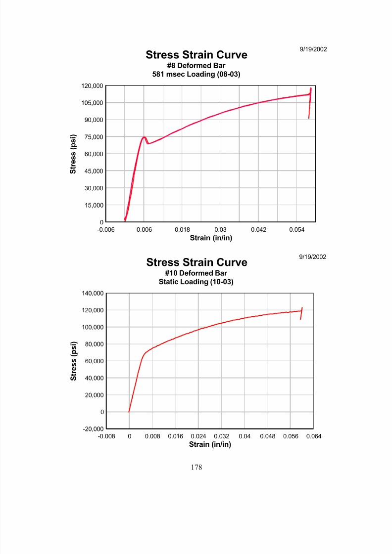
7/28/2019 Weathersby Dis
http://slidepdf.com/reader/full/weathersby-dis 195/280
178
9/19/2002
Strain (in/in)
S t r e s s ( p s i )
Stress Strain Curve#8 Deformed Bar
581 msec Loading (08-03)
-0.006 0.006 0.018 0.03 0.042 0.0540
15,000
30,000
45,000
60,000
75,000
90,000
105,000
120,000
9/19/2002
Strain (in/in)
S t r e s s ( p s i )
Stress Strain Curve#10 Deformed Bar
Static Loading (10-03)
-0.008 0 0.008 0.016 0.024 0.032 0.04 0.048 0.056 0.064-20,000
0
20,000
40,000
60,000
80,000
100,000
120,000
140,000
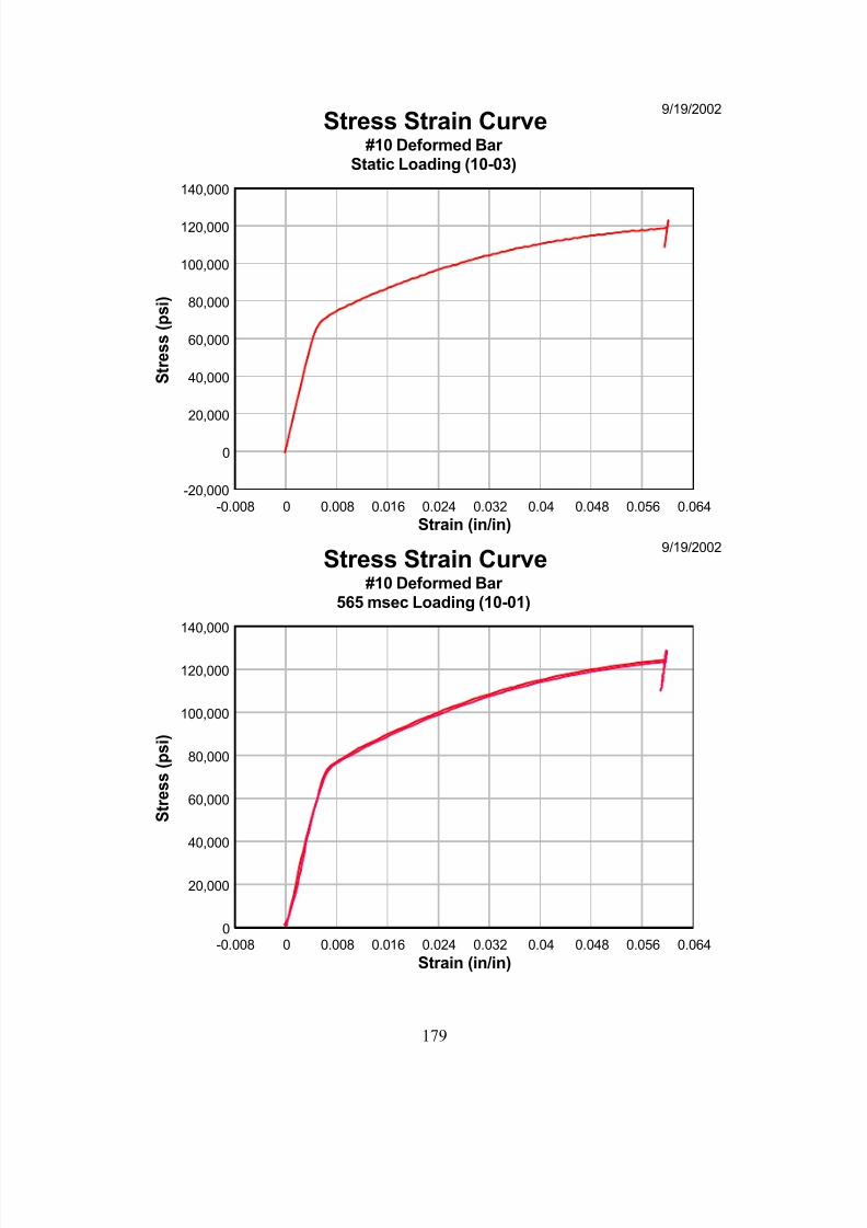
7/28/2019 Weathersby Dis
http://slidepdf.com/reader/full/weathersby-dis 196/280
179
9/19/2002
Strain (in/in)
S t r e s s ( p s i )
Stress Strain Curve#10 Deformed Bar
Static Loading (10-03)
-0.008 0 0.008 0.016 0.024 0.032 0.04 0.048 0.056 0.064-20,000
0
20,000
40,000
60,000
80,000
100,000
120,000
140,000
9/19/2002
Strain (in/in)
S t r e s s ( p s i )
Stress Strain Curve#10 Deformed Bar
565 msec Loading (10-01)
-0.008 0 0.008 0.016 0.024 0.032 0.04 0.048 0.056 0.0640
20,000
40,000
60,000
80,000
100,000
120,000
140,000

7/28/2019 Weathersby Dis
http://slidepdf.com/reader/full/weathersby-dis 197/280
180
APPENDIX B: SUMMARY OF TEST DATA
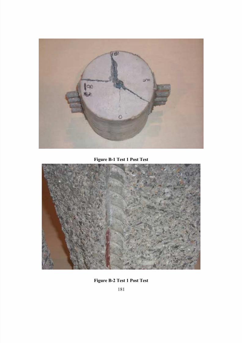
7/28/2019 Weathersby Dis
http://slidepdf.com/reader/full/weathersby-dis 198/280
181
Figure B-1 Test 1 Post Test
Figure B-2 Test 1 Post Test
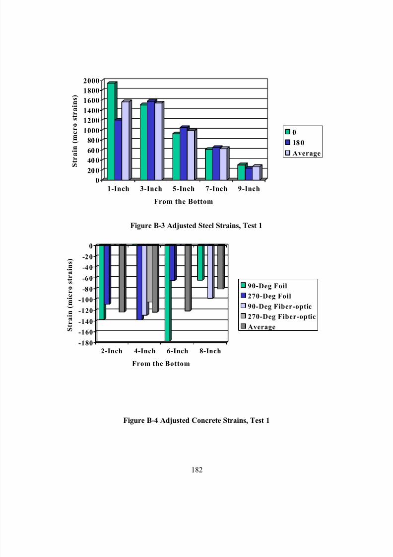
7/28/2019 Weathersby Dis
http://slidepdf.com/reader/full/weathersby-dis 199/280
182
0
200
400
600
800
1000
1200
1400
1600
1800
2000
S t r a i n ( m c r o s t r a i n s )
1-Inch 3-Inch 5-Inch 7-Inch 9-Inch
From the Bottom
0
180
Average
Figure B-3 Adjusted Steel Strains, Test 1
-180
-160
-140
-120
-100-80
-60
-40
-20
0
S t r a i n ( m i c r
o s t r a i n s )
2-Inch 4-Inch 6-Inch 8-Inch
From the Bottom
90-Deg Foil
270-Deg Foil
90-Deg Fiber-optic
270-Deg Fiber-optic
Average
Figure B-4 Adjusted Concrete Strains, Test 1
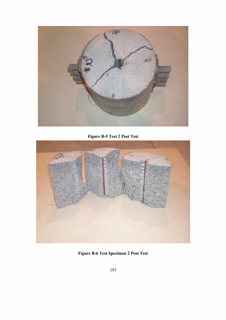
7/28/2019 Weathersby Dis
http://slidepdf.com/reader/full/weathersby-dis 200/280
183
Figure B-5 Test 2 Post Test
Figure B-6 Test Specimen 2 Post Test
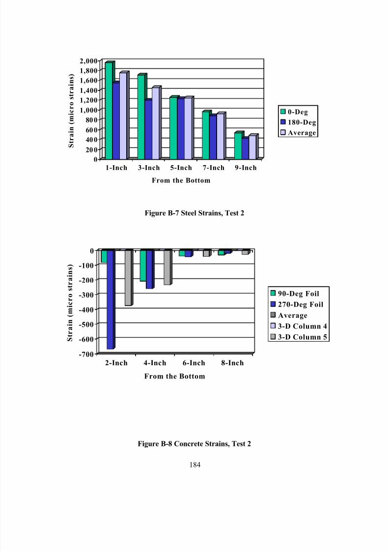
7/28/2019 Weathersby Dis
http://slidepdf.com/reader/full/weathersby-dis 201/280
184
0
200
400
600
800
1,000
1,200
1,400
1,600
1,800
2,000
S t r a i n ( m i c r o s t r a i n s )
1-Inch 3-Inch 5-Inch 7-Inch 9-Inch
From the Bottom
0-Deg
180-Deg
Average
Figure B-7 Steel Strains, Test 2
-700
-600
-500
-400
-300
-200
-100
0
S t r a i n ( m i c r o s
t r a i n s )
2-Inch 4-Inch 6-Inch 8-Inch
From the Bottom
90-Deg Foil
270-Deg Foil
Average
3-D Column 4
3-D Column 5
Figure B-8 Concrete Strains, Test 2
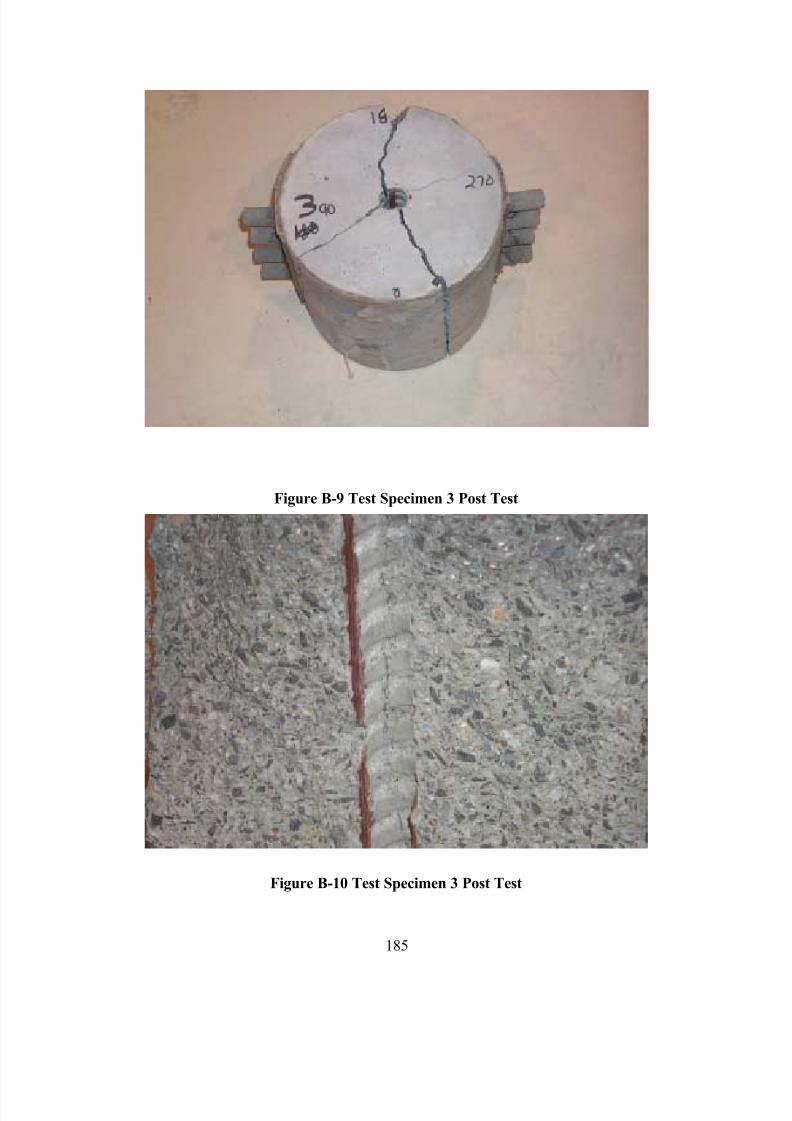
7/28/2019 Weathersby Dis
http://slidepdf.com/reader/full/weathersby-dis 202/280
185
Figure B-9 Test Specimen 3 Post Test
Figure B-10 Test Specimen 3 Post Test
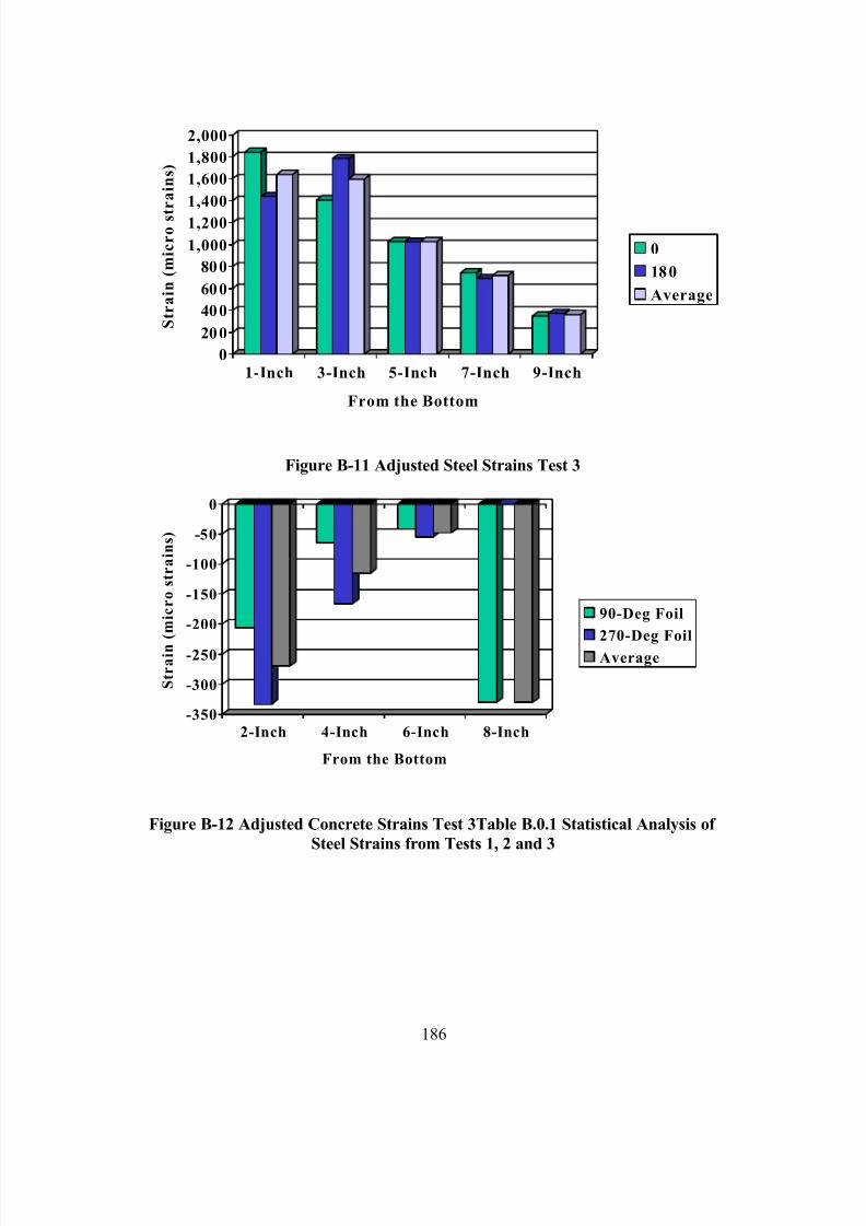
7/28/2019 Weathersby Dis
http://slidepdf.com/reader/full/weathersby-dis 203/280
186
0
200
400
600
800
1,000
1,200
1,400
1,600
1,800
2,000
S t r a i n ( m i c r o s t r a i n s )
1-Inch 3-Inch 5-Inch 7-Inch 9-Inch
From the Bottom
0
180
Average
Figure B-11 Adjusted Steel Strains Test 3
-350
-300
-250
-200
-150
-100
-50
0
S t r a i n
( m i c r o s t r a i n s )
2-Inch 4-Inch 6-Inch 8-Inch
From the Bottom
90-Deg Foil
270-Deg Foil
Average
Figure B-12 Adjusted Concrete Strains Test 3Table B.0.1 Statistical Analysis of
Steel Strains from Tests 1, 2 and 3
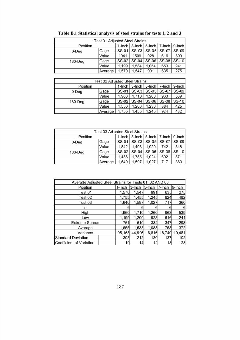
7/28/2019 Weathersby Dis
http://slidepdf.com/reader/full/weathersby-dis 204/280
187
Table B.1 Statistical analysis of steel strains for tests 1, 2 and 3
Test 01 Adjusted Steel Strains
Position 1-Inch 3-Inch 5-Inch 7-Inch 9-Inch
Gage SS-01 SS-03 SS-05 SS-07 SS-090-Deg
Value 1941 1509 928 616 309
Gage SS-02 SS-04 SS-06 SS-08 SS-10180-Deg
Value 1,199 1,584 1,054 653 241
Average 1,570 1,547 991 635 275
Test 02 Ad usted Steel Strains
Position 1-Inch 3-Inch 5-Inch 7-Inch 9-Inch
Gage SS-01 SS-03 SS-05 SS-07 SS-090-Deg
Value 1,960 1,710 1,260 963 539
Gage SS-02 SS-04 SS-06 SS-08 SS-10180-Deg
Value 1,550 1,200 1,230 884 425
Average 1,755 1,455 1,245 924 482
Test 03 Ad usted Steel Strains
Position 1-Inch 3-Inch 5-Inch 7-Inch 9-Inch
Gage SS-01 SS-03 SS-05 SS-07 SS-090-Deg
Value 1,842 1,408 1,029 742 348
Gage SS-02 SS-04 SS-06 SS-08 SS-10180-Deg
Value 1,438 1,785 1,024 692 371
Average 1,640 1,597 1,027 717 360
Avera e Ad usted Steel Strains for Tests 01, 02 AND 03
Position 1-Inch 3-Inch 5-Inch 7-Inch 9-Inch
Test 01 1,570 1,547 991 635 275
Test 02 1,755 1,455 1,245 924 482
Test 03 1,640 1,597 1,027 717 360
n 6 6 6 6 6
High 1,960 1,710 1,260 963 539
Low 1,199 1,200 928 616 241
Extreme Spread 761 510 332 347 298
Average 1,655 1,533 1,088 758 372
Variance 95,168 44,905 16,816 18,740 10,481
Standard Deviation 308 212 130 137 102Coefficient of Variation 19 14 12 18 28
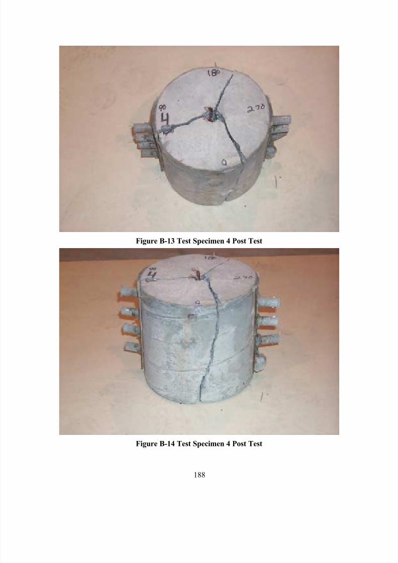
7/28/2019 Weathersby Dis
http://slidepdf.com/reader/full/weathersby-dis 205/280
188
Figure B-13 Test Specimen 4 Post Test
Figure B-14 Test Specimen 4 Post Test
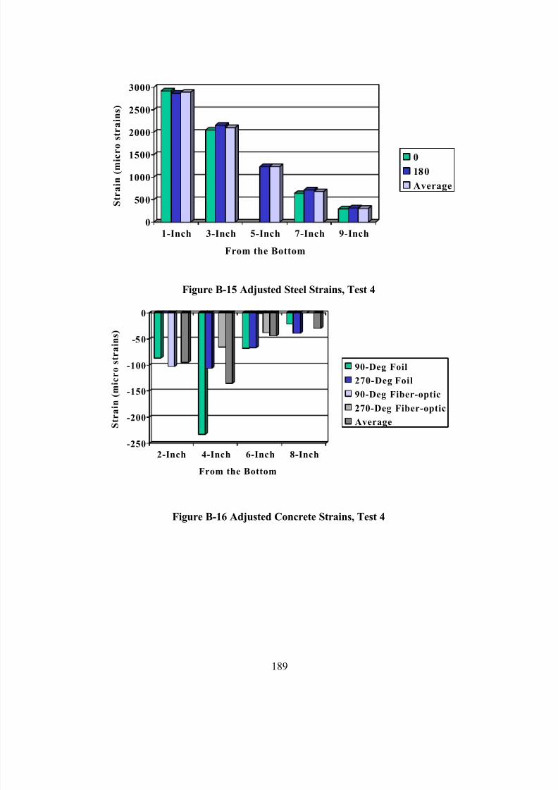
7/28/2019 Weathersby Dis
http://slidepdf.com/reader/full/weathersby-dis 206/280
189
0
500
1000
1500
2000
2500
3000
S t r a i n ( m i c r o s t r a i n s )
1-Inch 3-Inch 5-Inch 7-Inch 9-Inch
From the Bottom
0
180
Average
Figure B-15 Adjusted Steel Strains, Test 4
-250
-200
-150
-100
-50
0
S t r a i n ( m i c r o s t r a i n s )
2-Inch 4-Inch 6-Inch 8-Inch
From the Bottom
90-Deg Foil
270-Deg Foil
90-Deg Fiber-optic
270-Deg Fiber-optic
Average
Figure B-16 Adjusted Concrete Strains, Test 4
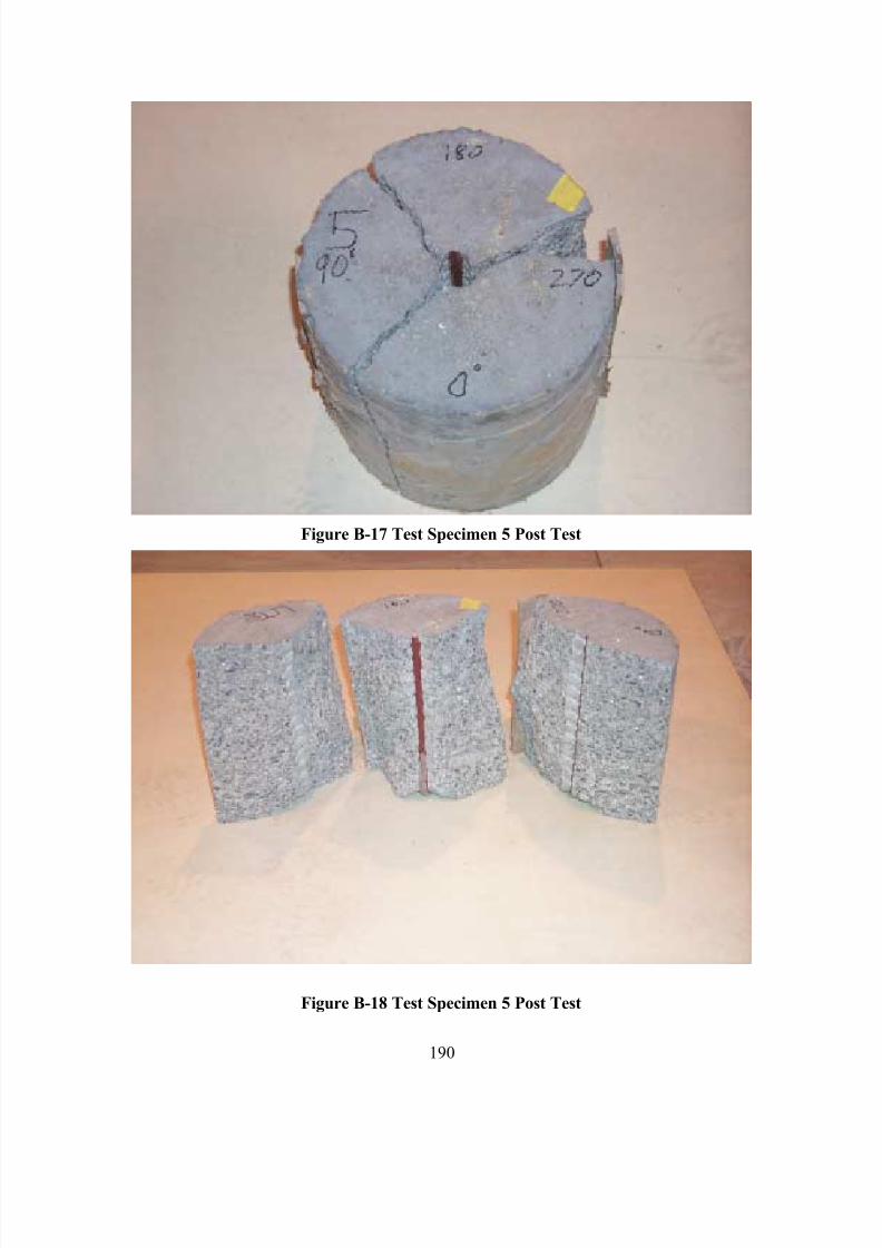
7/28/2019 Weathersby Dis
http://slidepdf.com/reader/full/weathersby-dis 207/280
190
Figure B-17 Test Specimen 5 Post Test
Figure B-18 Test Specimen 5 Post Test
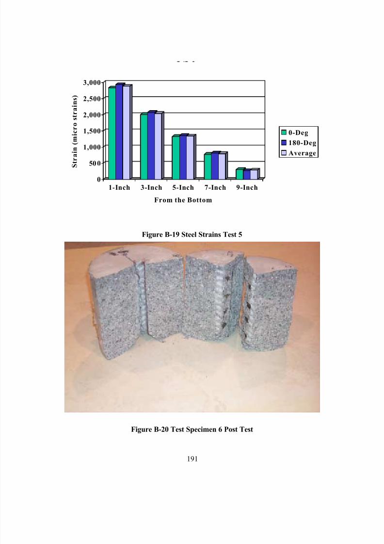
7/28/2019 Weathersby Dis
http://slidepdf.com/reader/full/weathersby-dis 208/280
191
0
500
1,000
1,500
2,000
2,500
3,000
S t r a i n ( m i c r o s t r a i n s )
1-Inch 3-Inch 5-Inch 7-Inch 9-InchFrom the Bottom
0-Deg
180-Deg
Average
Figure B-19 Steel Strains Test 5
Figure B-20 Test Specimen 6 Post Test
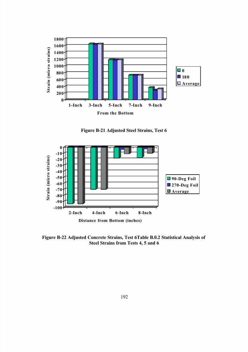
7/28/2019 Weathersby Dis
http://slidepdf.com/reader/full/weathersby-dis 209/280
192
0
200
400
600
800
10001200
1400
1600
1800
S t r a i n ( m i c r o s t r a i n s )
1-Inch 3-Inch 5-Inch 7-Inch 9-Inch
From the Bottom
0
180
Average
Figure B-21 Adjusted Steel Strains, Test 6
-100
-90
-80
-70-60
-50
-40
-30
-20
-10
0
S t r a i n ( m i c r o s t r a i n s )
2-Inch 4-Inch 6-Inch 8-Inch
Distance from Bottom (inches)
90-Deg Foil
270-Deg FoilAverage
Figure B-22 Adjusted Concrete Strains, Test 6Table B.0.2 Statistical Analysis of
Steel Strains from Tests 4, 5 and 6
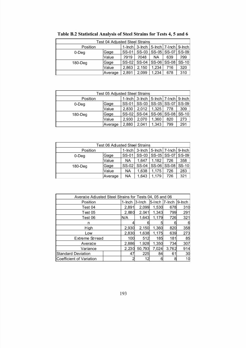
7/28/2019 Weathersby Dis
http://slidepdf.com/reader/full/weathersby-dis 210/280
193
Table B.2 Statistical Analysis of Steel Strains for Tests 4, 5 and 6
Test 04 Adjusted Steel Strains
Position 1-Inch 3-Inch 5-Inch 7-Inch 9-Inch
Gage SS-01 SS-03 SS-05 SS-07 SS-090-Deg
Value 2919 2048 NA 639 299
Gage SS-02 SS-04 SS-06 SS-08 SS-10180-Deg
Value 2,863 2,150 1,234 716 320
Average 2,891 2,099 1,234 678 310
Test 05 Adjusted Steel Strains
Position 1-Inch 3-Inch 5-Inch 7-Inch 9-Inch
Gage SS-01 SS-03 SS-05 SS-07 SS-090-Deg
Value 2,830 2,012 1,325 778 309
Gage SS-02 SS-04 SS-06 SS-08 SS-10180-Deg
Value 2,930 2,070 1,360 820 273
Average 2,880 2,041 1,343 799 291
Test 06 Ad usted Steel Strains
Position 1-Inch 3-Inch 5-Inch 7-Inch 9-Inch
Gage SS-01 SS-03 SS-05 SS-07 SS-090-Deg
Value NA 1,647 1,182 726 358
Gage SS-02 SS-04 SS-06 SS-08 SS-10180-Deg
Value NA 1,638 1,175 726 283
Average NA 1,643 1,179 726 321
Avera e Ad usted Steel Strains for Tests 04, 05 and 06
Position 1-Inch 3-Inch 5-Inch 7-Inch 9-Inch
Test 04 2,891 2,099 1,530 678 310
Test 05 2,880 2,041 1,343 799 291
Test 06 N/A 1,643 1,179 726 321
n 4 6 5 6 6
High 2,930 2,150 1,360 820 358
Low 2,830 1,638 1,175 639 273
Extreme S read 100 512 185 181 85
Avera e 2,886 1,928 1,350 734 307Variance 2,230 50,793 7,024 3,762 914
Standard Deviation 47 225 84 61 30
Coefficient of Variation 2 12 6 8 10
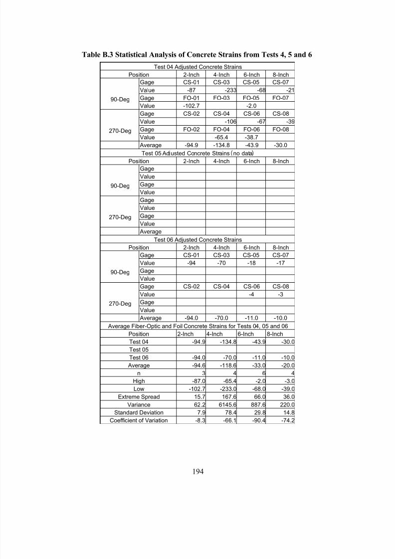
7/28/2019 Weathersby Dis
http://slidepdf.com/reader/full/weathersby-dis 211/280
194
Table B.3 Statistical Analysis of Concrete Strains from Tests 4, 5 and 6
Test 04 Adjusted Concrete Strains
Position 2-Inch 4-Inch 6-Inch 8-Inch
Gage CS-01 CS-03 CS-05 CS-07
Value -87 -233 -68 -21
Gage FO-01 FO-03 FO-05 FO-0790-DegValue -102.7 -2.0
Gage CS-02 CS-04 CS-06 CS-08
Value -106 -67 -39
Gage FO-02 FO-04 FO-06 FO-08270-DegValue -65.4 -38.7
Average -94.9 -134.8 -43.9 -30.0
Test 05 Ad usted Concrete Strains no data
Position 2-Inch 4-Inch 6-Inch 8-Inch
Gage
Value
Gage90-DegValue
Gage
Value
Gage270-DegValue
Average
Test 06 Adjusted Concrete Strains
Position 2-Inch 4-Inch 6-Inch 8-Inch
Gage CS-01 CS-03 CS-05 CS-07
Value -94 -70 -18 -17
Gage90-DegValue
Gage CS-02 CS-04 CS-06 CS-08
Value -4 -3Gage270-DegValue
Average -94.0 -70.0 -11.0 -10.0
Average Fiber-Optic and Foil Concrete Strains for Tests 04, 05 and 06
Position 2-Inch 4-Inch 6-Inch 8-Inch
Test 04 -94.9 -134.8 -43.9 -30.0
Test 05
Test 06 -94.0 -70.0 -11.0 -10.0
Average -94.6 -118.6 -33.0 -20.0
n 3 4 6 4
High -87.0 -65.4 -2.0 -3.0
Low -102.7 -233.0 -68.0 -39.0Extreme Spread 15.7 167.6 66.0 36.0
Variance 62.2 6145.6 887.6 220.0
Standard Deviation 7.9 78.4 29.8 14.8
Coefficient of Variation -8.3 -66.1 -90.4 -74.2
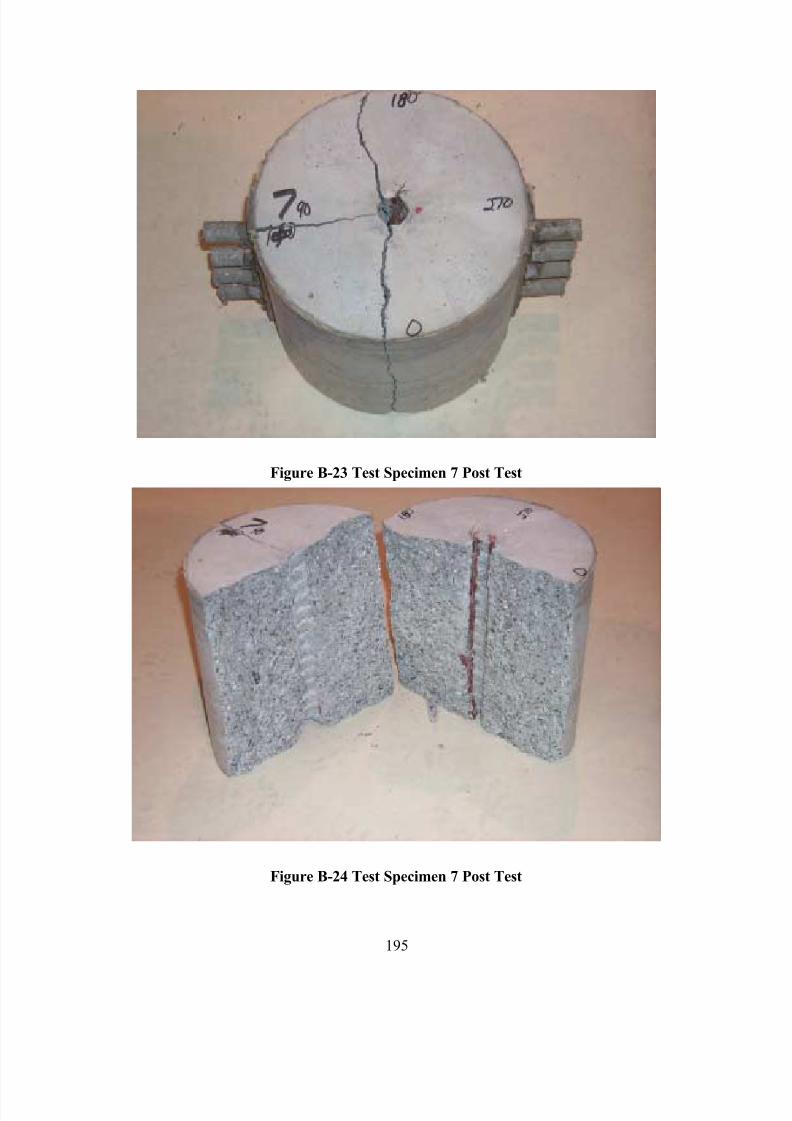
7/28/2019 Weathersby Dis
http://slidepdf.com/reader/full/weathersby-dis 212/280
195
Figure B-23 Test Specimen 7 Post Test
Figure B-24 Test Specimen 7 Post Test
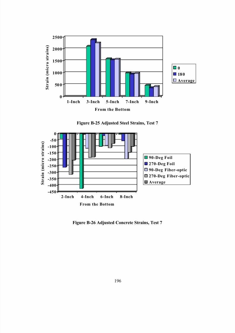
7/28/2019 Weathersby Dis
http://slidepdf.com/reader/full/weathersby-dis 213/280
196
0
500
1000
1500
2000
2500
S t r a i n ( m i c r o s t
r a i n s )
1-Inch 3-Inch 5-Inch 7-Inch 9-Inch
From the Bottom
0
180
Average
Figure B-25 Adjusted Steel Strains, Test 7
-450
-400
-350
-300
-250
-200
-150
-100
-50
0
S t r a i n ( m i c r o s t r a i n s )
2-Inch 4-Inch 6-Inch 8-Inch
From the Bottom
90-Deg Foil
270-Deg Foil
90-Deg Fiber-optic
270-Deg Fiber-optic
Average
Figure B-26 Adjusted Concrete Strains, Test 7
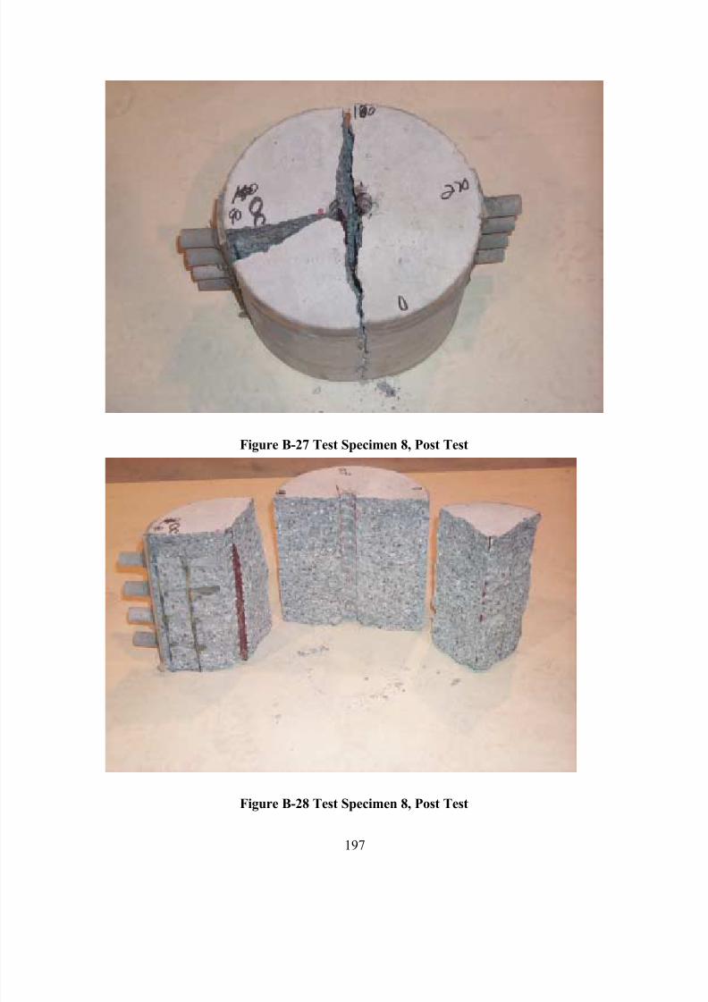
7/28/2019 Weathersby Dis
http://slidepdf.com/reader/full/weathersby-dis 214/280
197
Figure B-27 Test Specimen 8, Post Test
Figure B-28 Test Specimen 8, Post Test
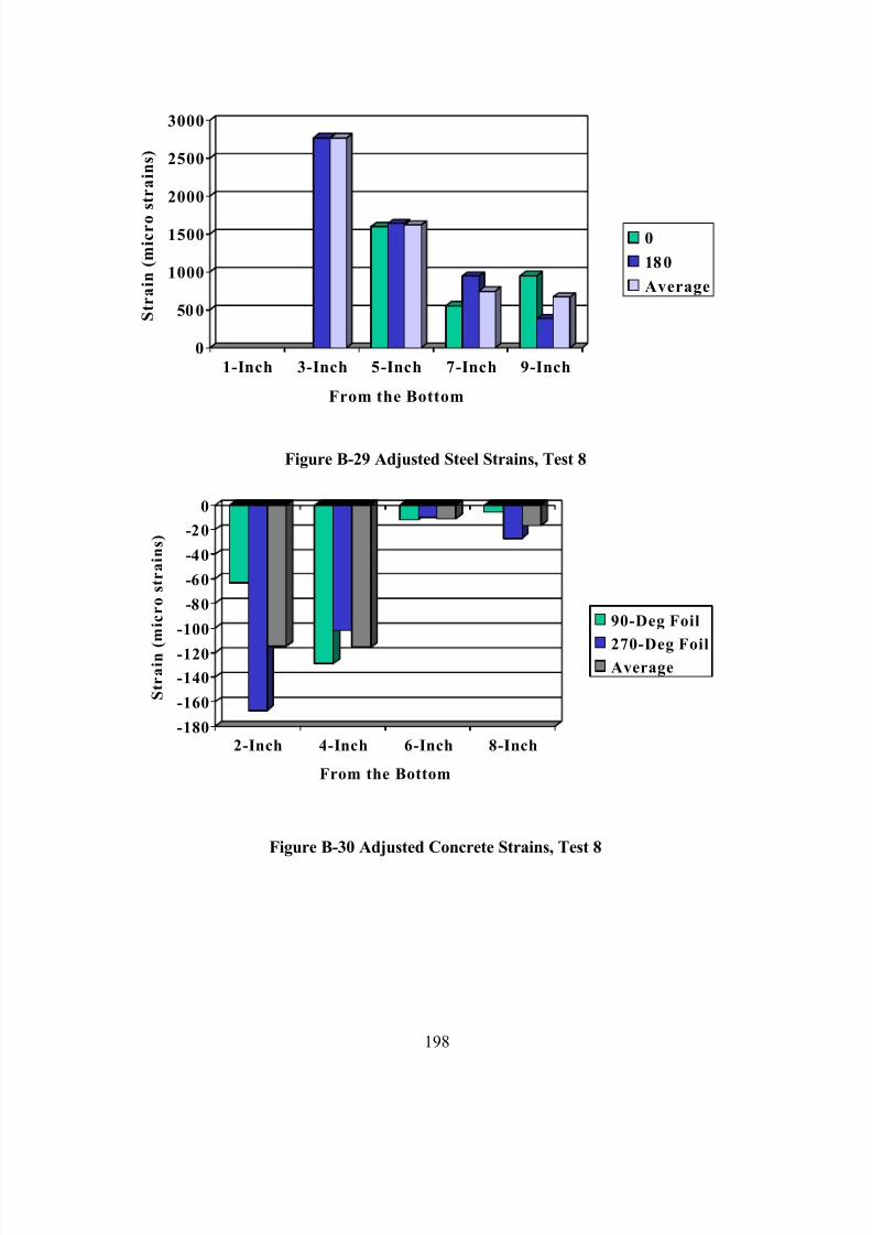
7/28/2019 Weathersby Dis
http://slidepdf.com/reader/full/weathersby-dis 215/280
198
0
500
1000
1500
2000
2500
3000
S t r a i n ( m i c r o
s t r a i n s )
1-Inch 3-Inch 5-Inch 7-Inch 9-Inch
From the Bottom
0
180
Average
Figure B-29 Adjusted Steel Strains, Test 8
-180
-160
-140
-120
-100
-80
-60
-40
-20
0
S t r a i n ( m i c r o s t r a i n s )
2-Inch 4-Inch 6-Inch 8-Inch
From the Bottom
90-Deg Foil
270-Deg FoilAverage
Figure B-30 Adjusted Concrete Strains, Test 8
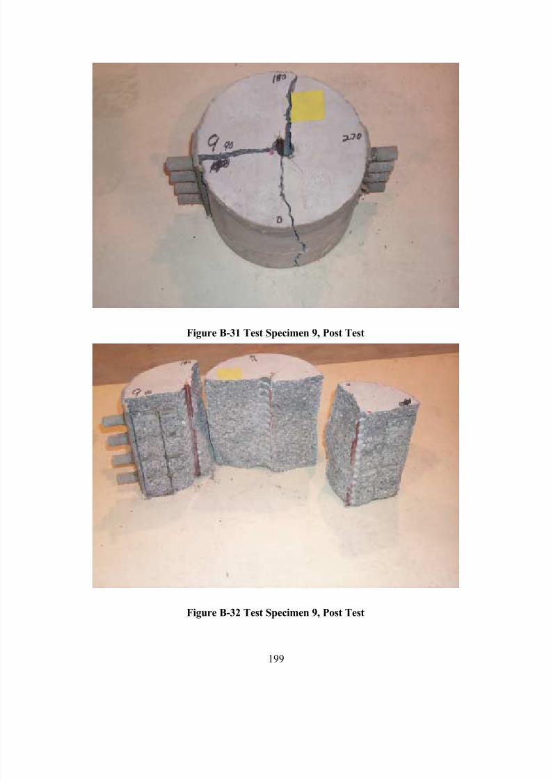
7/28/2019 Weathersby Dis
http://slidepdf.com/reader/full/weathersby-dis 216/280
199
Figure B-31 Test Specimen 9, Post Test
Figure B-32 Test Specimen 9, Post Test
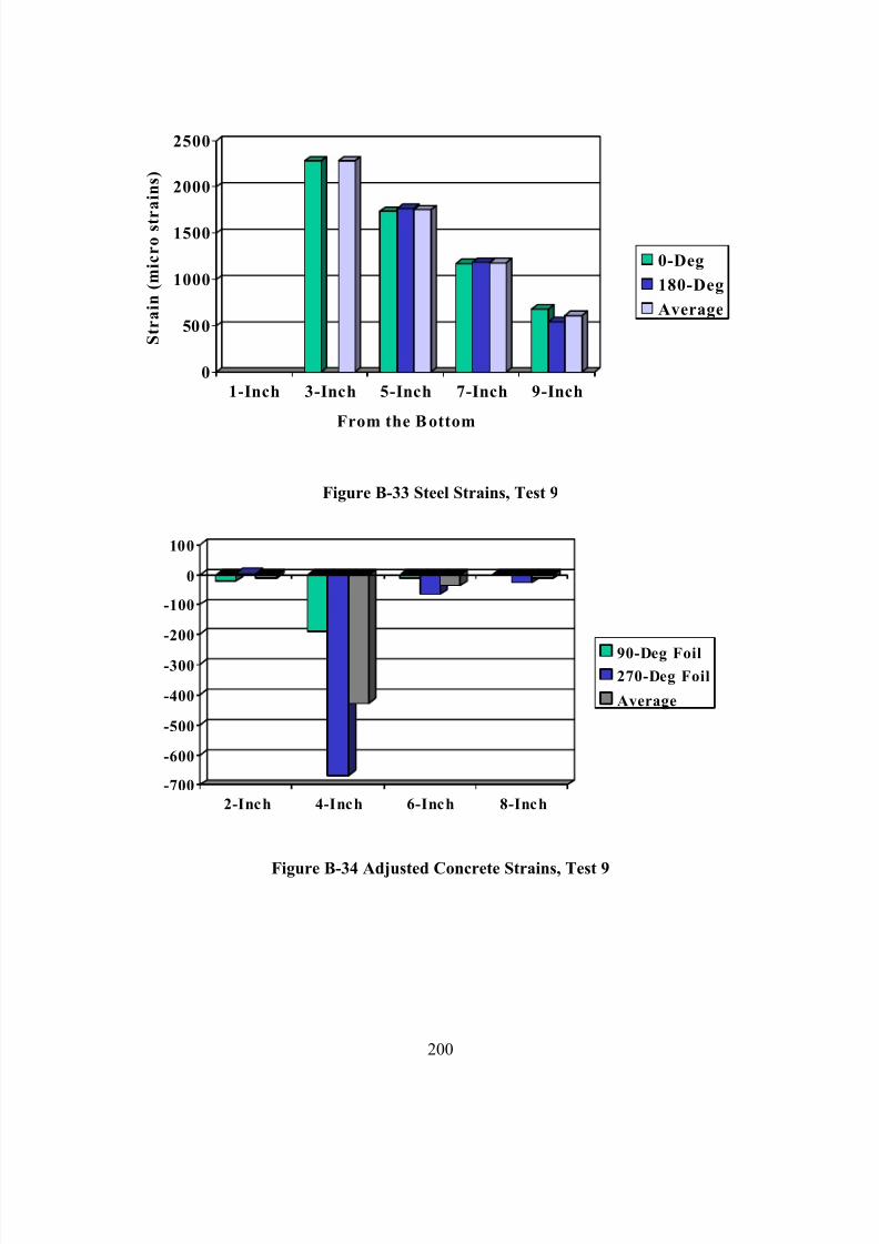
7/28/2019 Weathersby Dis
http://slidepdf.com/reader/full/weathersby-dis 217/280
200
0
500
1000
1500
2000
2500
S t r a i n ( m i c r o s t r
a i n s )
1-Inch 3-Inch 5-Inch 7-Inch 9-Inch
From the B ottom
0-Deg
180-Deg
Average
Figure B-33 Steel Strains, Test 9
-700
-600
-500
-400
-300
-200
-100
0
100
2-Inch 4-Inch 6-Inch 8-Inch
90-Deg Foil270-Deg Foil
Average
Figure B-34 Adjusted Concrete Strains, Test 9

7/28/2019 Weathersby Dis
http://slidepdf.com/reader/full/weathersby-dis 218/280
201
Table B.4 Statistical Analysis of Steel Strains for Tests 7, 8 and 9
Test 07 Adjusted Steel Strains
Position 1-Inch 3-Inch 5-Inch 7-Inch 9-Inch
Gage SS-01 SS-03 SS-05 SS-07 SS-090-Deg
Value N/A 2,108 1,581 990 470
Gage SS-02 SS-04 SS-06 SS-08 SS-10180-Deg
Value NA 2,386 1,544 950 367
Average N/A 2,247 1,563 970 419
Test 08 Adjusted Steel Strains
Position 1-Inch 3-Inch 5-Inch 7-Inch 9-Inch
Gage SS-01 SS-03 SS-05 SS-07 SS-090-Deg
Value N/A N/A 1,599 550 950
Gage SS-02 SS-04 SS-06 SS-08 SS-10180-Deg
Value N/A 2,762 1,637 946 386
Average N/A 2,762 1,618 748 668
Test 09 Ad usted Steel Strains
Position 1-Inch 3-Inch 5-Inch 7-Inch 9-Inch
Gage SS-01 SS-03 SS-05 SS-07 SS-090-Deg
Value N/A 2,280 1,740 1,175 680
Gage SS-02 SS-04 SS-06 SS-08 SS-10180-Deg
Value N/A N/A 1,770 1,185 545
Average N/A 2,280 1,755 1,180 613
Avera e Ad usted Steel Strains for Tests 07, 08 AND 09
Position 1-Inch 3-Inch 5-Inch 7-Inch 9-Inch
Test 07 N/A 2,247 1,563 970 419
Test 08 N/A 2,762 1,618 748 668
Test 09 N/A 2,280 1,755 1,180 613
n 0 4 6 6 6
High N/A 2,762 1,770 1,185 950
Low N/A 2,108 1,544 550 367
Extreme S read N/A 654 226 635 583
Avera e N/A 2,384 1,645 966 566Variance N/A 76,627 8,225 53,186 48,422
Standard Deviation N/A 277 91 231 220
Coefficient of Variation N/A 12 6 24 39
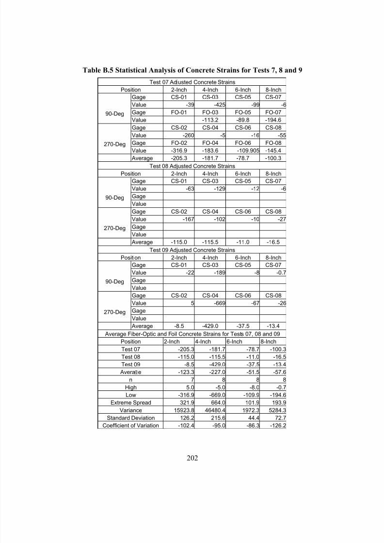
7/28/2019 Weathersby Dis
http://slidepdf.com/reader/full/weathersby-dis 219/280
202
Table B.5 Statistical Analysis of Concrete Strains for Tests 7, 8 and 9
Test 07 Ad usted Concrete Strains
Position 2-Inch 4-Inch 6-Inch 8-Inch
Gage CS-01 CS-03 CS-05 CS-07
Value -39 -425 -99 -6
Gage FO-01 FO-03 FO-05 FO-0790-DegValue -113.2 -89.8 -194.6
Gage CS-02 CS-04 CS-06 CS-08
Value -260 -5 -16 -55
Gage FO-02 FO-04 FO-06 FO-08270-DegValue -316.9 -183.6 -109.905 -145.4
Average -205.3 -181.7 -78.7 -100.3
Test 08 Adjusted Concrete Strains
Position 2-Inch 4-Inch 6-Inch 8-Inch
Gage CS-01 CS-03 CS-05 CS-07
Value -63 -129 -12 -6Gage90-DegValue
Gage CS-02 CS-04 CS-06 CS-08
Value -167 -102 -10 -27
Gage270-DegValue
Average -115.0 -115.5 -11.0 -16.5
Test 09 Adjusted Concrete Strains
Position 2-Inch 4-Inch 6-Inch 8-Inch
Gage CS-01 CS-03 CS-05 CS-07
Value -22 -189 -8 -0.7
Gage90-DegValue
Gage CS-02 CS-04 CS-06 CS-08
Value 5 -669 -67 -26
Gage270-DegValue
Average -8.5 -429.0 -37.5 -13.4
Average Fiber-Optic and Foil Concrete Strains for Tests 07, 08 and 09
Position 2-Inch 4-Inch 6-Inch 8-Inch
Test 07 -205.3 -181.7 -78.7 -100.3
Test 08 -115.0 -115.5 -11.0 -16.5
Test 09 -8.5 -429.0 -37.5 -13.4
Avera e -123.3 -227.0 -51.5 -57.6
n 7 8 8 8High 5.0 -5.0 -8.0 -0.7
Low -316.9 -669.0 -109.9 -194.6
Extreme Spread 321.9 664.0 101.9 193.9
Variance 15923.8 46480.4 1972.3 5284.3
Standard Deviation 126.2 215.6 44.4 72.7
Coefficient of Variation -102.4 -95.0 -86.3 -126.2
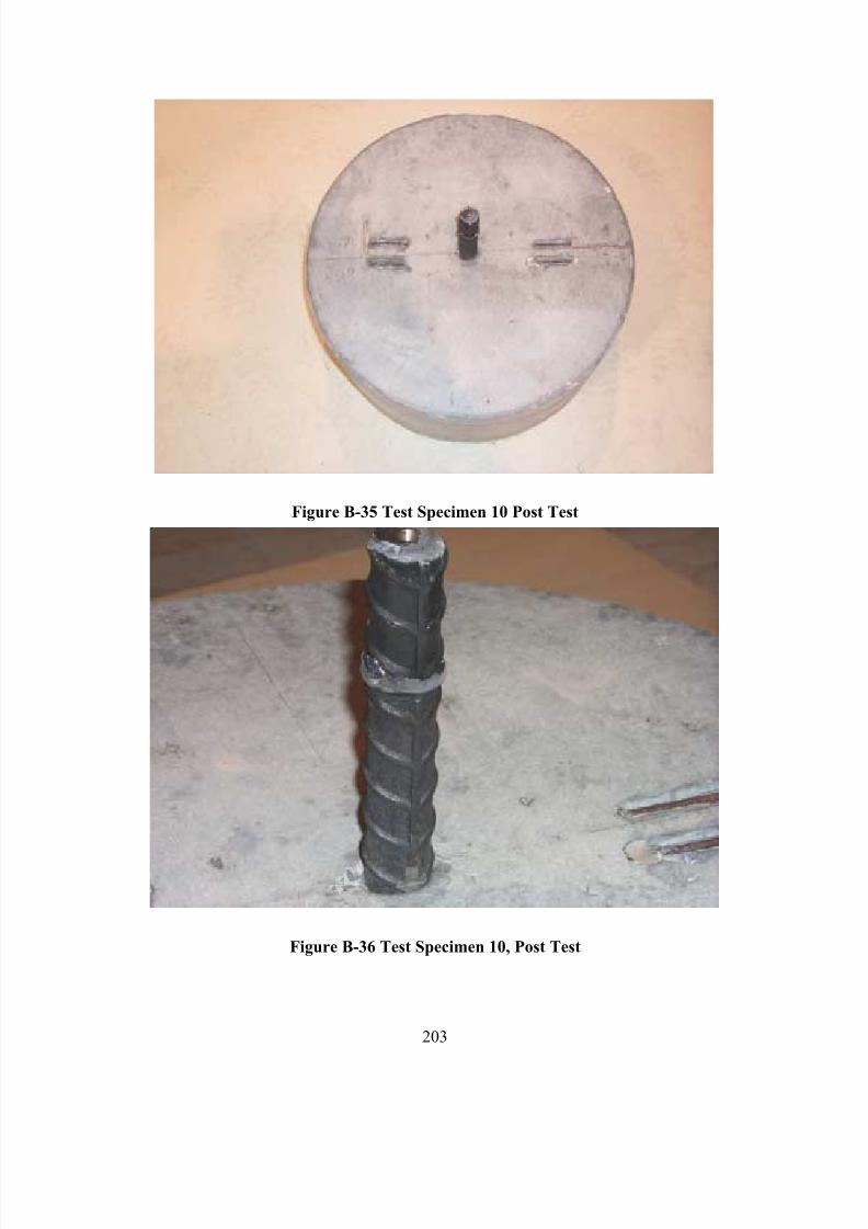
7/28/2019 Weathersby Dis
http://slidepdf.com/reader/full/weathersby-dis 220/280
203
Figure B-35 Test Specimen 10 Post Test
Figure B-36 Test Specimen 10, Post Test
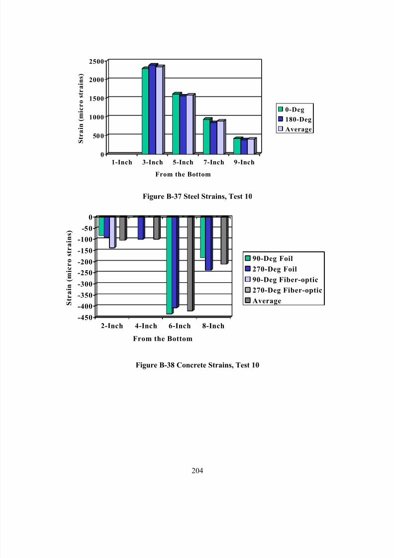
7/28/2019 Weathersby Dis
http://slidepdf.com/reader/full/weathersby-dis 221/280
204
0
500
1000
1500
2000
2500
S t r a i n ( m i c r o s
t r a i n s )
1-Inch 3-Inch 5-Inch 7-Inch 9-Inch
From the Bottom
0-Deg
180-Deg
Average
Figure B-37 Steel Strains, Test 10
-450
-400
-350
-300
-250
-200
-150
-100
-50
0
S t r a
i n ( m i c r o s t r a i n s )
2-Inch 4-Inch 6-Inch 8-Inch
From the Bottom
90-Deg Foil
270-Deg Foil
90-Deg Fiber-optic
270-Deg Fiber-opticAverage
Figure B-38 Concrete Strains, Test 10
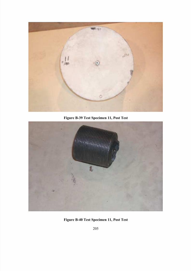
7/28/2019 Weathersby Dis
http://slidepdf.com/reader/full/weathersby-dis 222/280
205
Figure B-39 Test Specimen 11, Post Test
Figure B-40 Test Specimen 11, Post Test
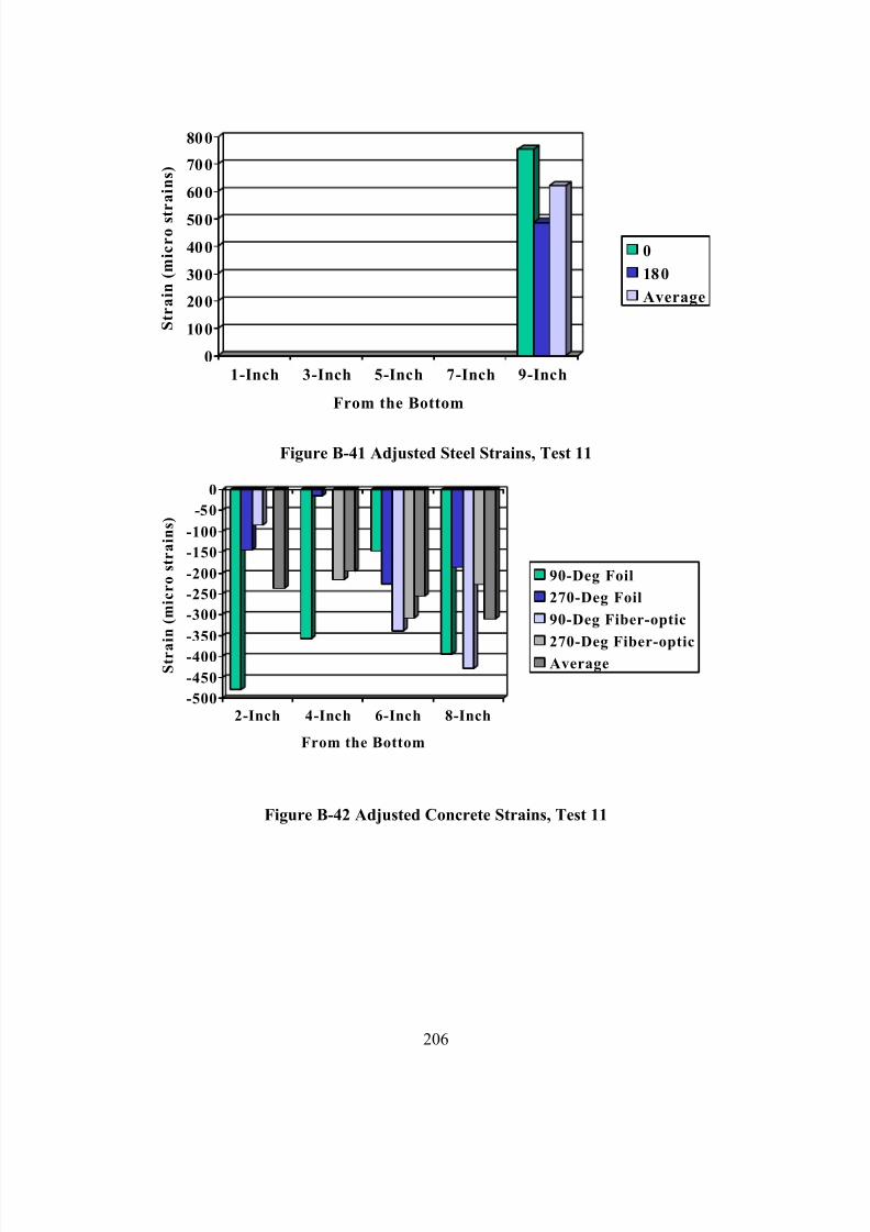
7/28/2019 Weathersby Dis
http://slidepdf.com/reader/full/weathersby-dis 223/280
206
0
100
200
300
400
500
600
700
800
S t r a i n ( m i c r o s t
r a i n s )
1-Inch 3-Inch 5-Inch 7-Inch 9-Inch
From the Bottom
0
180
Average
Figure B-41 Adjusted Steel Strains, Test 11
-500
-450
-400
-350
-300
-250
-200
-150
-100
-50
0
S t r a
i n ( m i c r o s t r a i n s )
2-Inch 4-Inch 6-Inch 8-Inch
From the Bottom
90-Deg Foil
270-Deg Foil
90-Deg Fiber-optic
270-Deg Fiber-opticAverage
Figure B-42 Adjusted Concrete Strains, Test 11
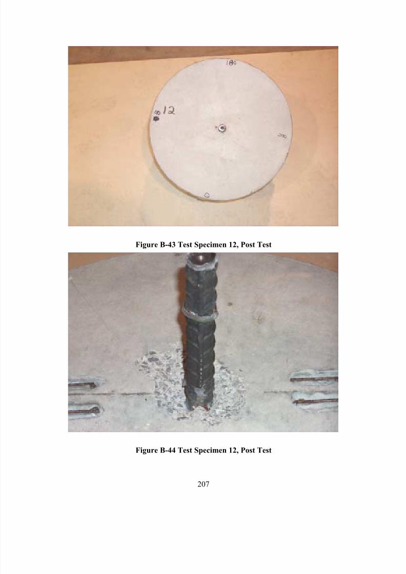
7/28/2019 Weathersby Dis
http://slidepdf.com/reader/full/weathersby-dis 224/280
207
Figure B-43 Test Specimen 12, Post Test
Figure B-44 Test Specimen 12, Post Test
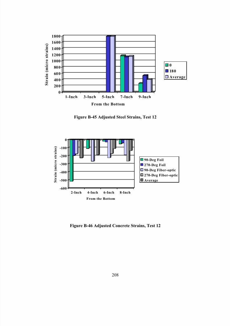
7/28/2019 Weathersby Dis
http://slidepdf.com/reader/full/weathersby-dis 225/280
208
0
200
400
600
800
10001200
1400
1600
1800
S t r a i n ( m i c r o s t r a i n s )
1-Inch 3-Inch 5-Inch 7-Inch 9-Inch
From the Bottom
0
180
Average
Figure B-45 Adjusted Steel Strains, Test 12
-600
-500
-400
-300
-200
-100
0
S t r a i n ( m i c r o s t r a i n s )
2-Inch 4-Inch 6-Inch 8-Inch
From the Bottom
90-Deg Foil
270-Deg Foil
90-Deg Fiber-optic270-Deg Fiber-optic
Average
Figure B-46 Adjusted Concrete Strains, Test 12

7/28/2019 Weathersby Dis
http://slidepdf.com/reader/full/weathersby-dis 226/280
209
Table B.6 Statistical Analysis of Steel Strains for Tests 10, 11 and 12
Test 10 Adjusted Steel Strains
Position 1-Inch 3-Inch 5-Inch 7-Inch 9-Inch
Gage SS-01 SS-03 SS-05 SS-07 SS-090-Deg
Value N/A 2,300 1,614 935 421
Gage SS-02 SS-04 SS-06 SS-08 SS-10180-Deg
Value N/A 2,390 1,560 845 390
Average N/A 2,345 1,587 890 406
Test 11 Adjusted Steel Strains
Position 1-Inch 3-Inch 5-Inch 7-Inch 9-Inch
Gage SS-01 SS-03 SS-05 SS-07 SS-090-Deg
Value N/A N/A N/A N/A 754
Gage SS-02 SS-04 SS-06 SS-08 SS-10180-Deg
Value N/A N/A N/A N/A 487
Average N/A N/A N/A N/A 621
Test 12 Ad usted Steel Strains
Position 1-Inch 3-Inch 5-Inch 7-Inch 9-Inch
Gage SS-01 SS-03 SS-05 SS-07 SS-090-Deg
Value N/A N/A N/A 1,168 282
Gage SS-02 SS-04 SS-06 SS-08 SS-10180-Deg
Value N/A N/A 1,790 1,132 534
Average N/A N/A 1,790 1,150 408
Avera e Ad usted Steel Strains for Tests 10, 11 and 12
Position 1-Inch 3-Inch 5-Inch 7-Inch 9-Inch
Test 10 N/A 2,345 1,587 890 406
Test 11 N/A N/A N/A N/A 621
Test 12 N/A N/A 1,790 1,150 408
n 0 2 3 4 6
High N/A 2,390 1,790 1,168 754
Low N/A 2,300 1,560 845 282
Extreme S read N/A 90 230 323 472
Avera e N/A 2,345 1,655 1,020 478Variance N/A N/A 14,465 24,099 25,760
Standard Deviation N/A N/A 120 155 161
Coefficient of Variation N/A N/A 7 15 34
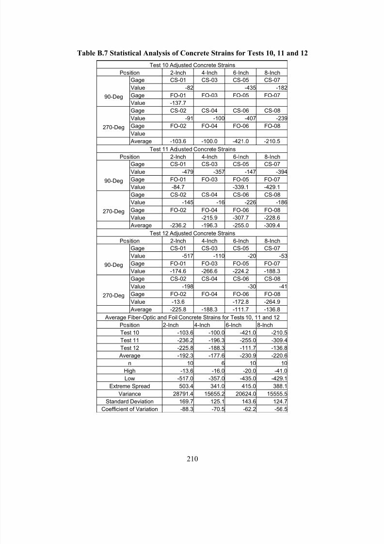
7/28/2019 Weathersby Dis
http://slidepdf.com/reader/full/weathersby-dis 227/280
210
Table B.7 Statistical Analysis of Concrete Strains for Tests 10, 11 and 12
Test 10 Adjusted Concrete Strains
Position 2-Inch 4-Inch 6-Inch 8-Inch
Gage CS-01 CS-03 CS-05 CS-07
Value -82 -435 -182
Gage FO-01 FO-03 FO-05 FO-0790-DegValue -137.7
Gage CS-02 CS-04 CS-06 CS-08
Value -91 -100 -407 -239
Gage FO-02 FO-04 FO-06 FO-08270-DegValue
Average -103.6 -100.0 -421.0 -210.5
Test 11 Ad usted Concrete Strains
Position 2-Inch 4-Inch 6-Inch 8-Inch
Gage CS-01 CS-03 CS-05 CS-07
Value -479 -357 -147 -394
Gage FO-01 FO-03 FO-05 FO-0790-DegValue -84.7 -339.1 -429.1
Gage CS-02 CS-04 CS-06 CS-08
Value -145 -16 -226 -186
Gage FO-02 FO-04 FO-06 FO-08270-DegValue -215.9 -307.7 -228.6
Average -236.2 -196.3 -255.0 -309.4
Test 12 Adjusted Concrete Strains
Position 2-Inch 4-Inch 6-Inch 8-Inch
Gage CS-01 CS-03 CS-05 CS-07
Value -517 -110 -20 -53
Gage FO-01 FO-03 FO-05 FO-0790-DegValue -174.6 -266.6 -224.2 -188.3
Gage CS-02 CS-04 CS-06 CS-08
Value -198 -30 -41 Gage FO-02 FO-04 FO-06 FO-08270-DegValue -13.6 -172.8 -264.9
Average -225.8 -188.3 -111.7 -136.8
Average Fiber-Optic and Foil Concrete Strains for Tests 10, 11 and 12
Position 2-Inch 4-Inch 6-Inch 8-Inch
Test 10 -103.6 -100.0 -421.0 -210.5
Test 11 -236.2 -196.3 -255.0 -309.4
Test 12 -225.8 -188.3 -111.7 -136.8
Average -192.3 -177.6 -230.9 -220.6
n 10 6 10 10
High -13.6 -16.0 -20.0 -41.0
Low -517.0 -357.0 -435.0 -429.
1 Extreme Spread 503.4 341.0 415.0 388.1
Variance 28791.4 15655.2 20624.0 15555.5
Standard Deviation 169.7 125.1 143.6 124.7
Coefficient of Variation -88.3 -70.5 -62.2 -56.5
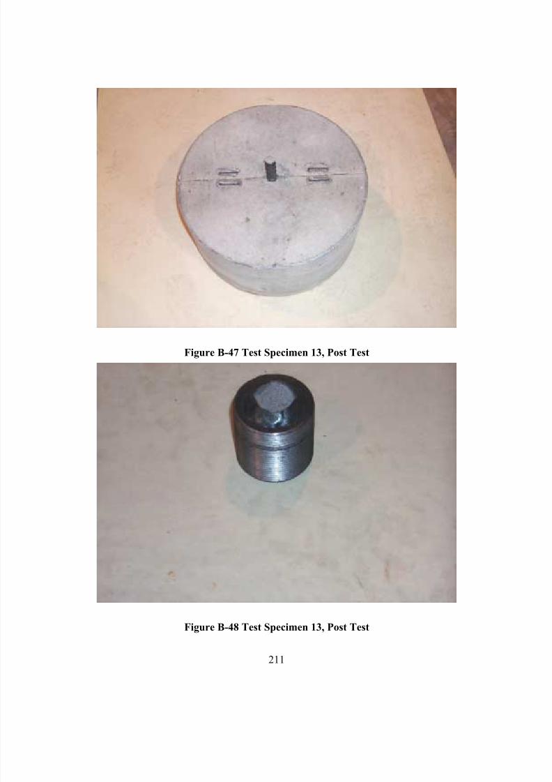
7/28/2019 Weathersby Dis
http://slidepdf.com/reader/full/weathersby-dis 228/280
211
Figure B-47 Test Specimen 13, Post Test
Figure B-48 Test Specimen 13, Post Test
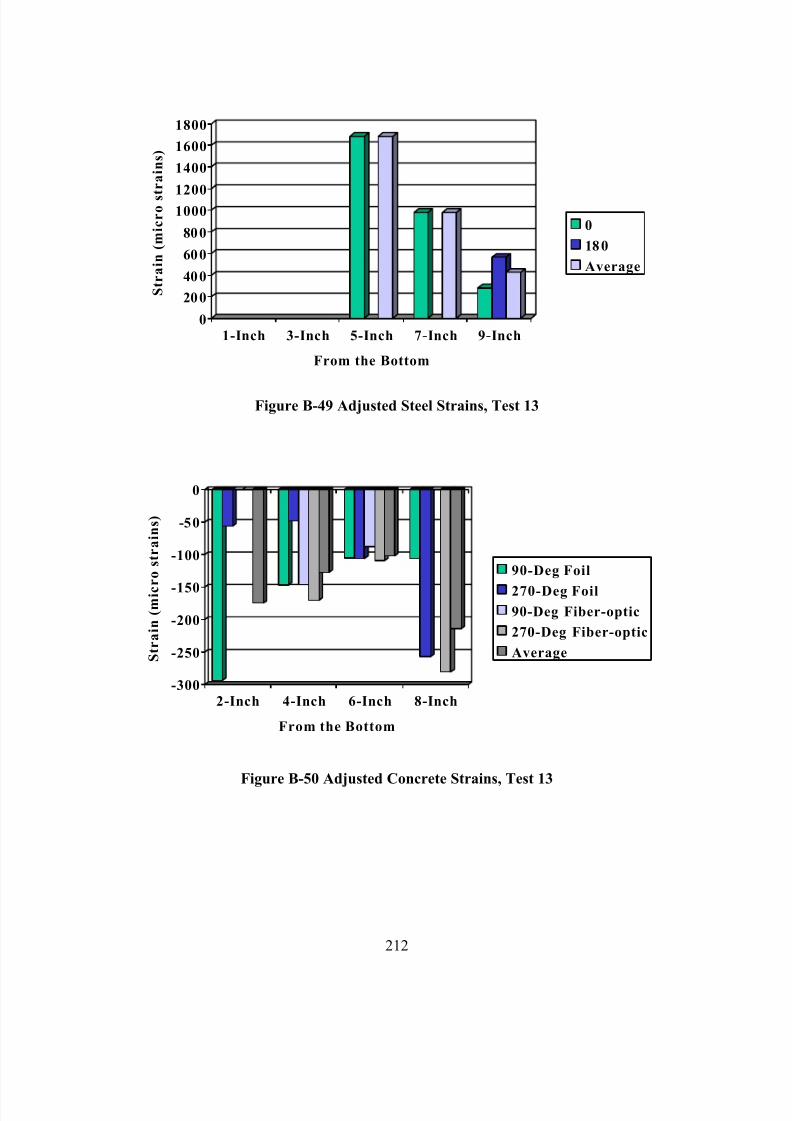
7/28/2019 Weathersby Dis
http://slidepdf.com/reader/full/weathersby-dis 229/280
212
0
200
400
600
800
10001200
1400
1600
1800
S t r a i n ( m i c r o s t r a i n s )
1-Inch 3-Inch 5-Inch 7-Inch 9-Inch
From the Bottom
0
180
Average
Figure B-49 Adjusted Steel Strains, Test 13
-300
-250
-200
-150
-100
-50
0
S t r a i n ( m i c
r o s t r a i n s )
2-Inch 4-Inch 6-Inch 8-Inch
From the Bottom
90-Deg Foil
270-Deg Foil
90-Deg Fiber-optic
270-Deg Fiber-optic
Average
Figure B-50 Adjusted Concrete Strains, Test 13
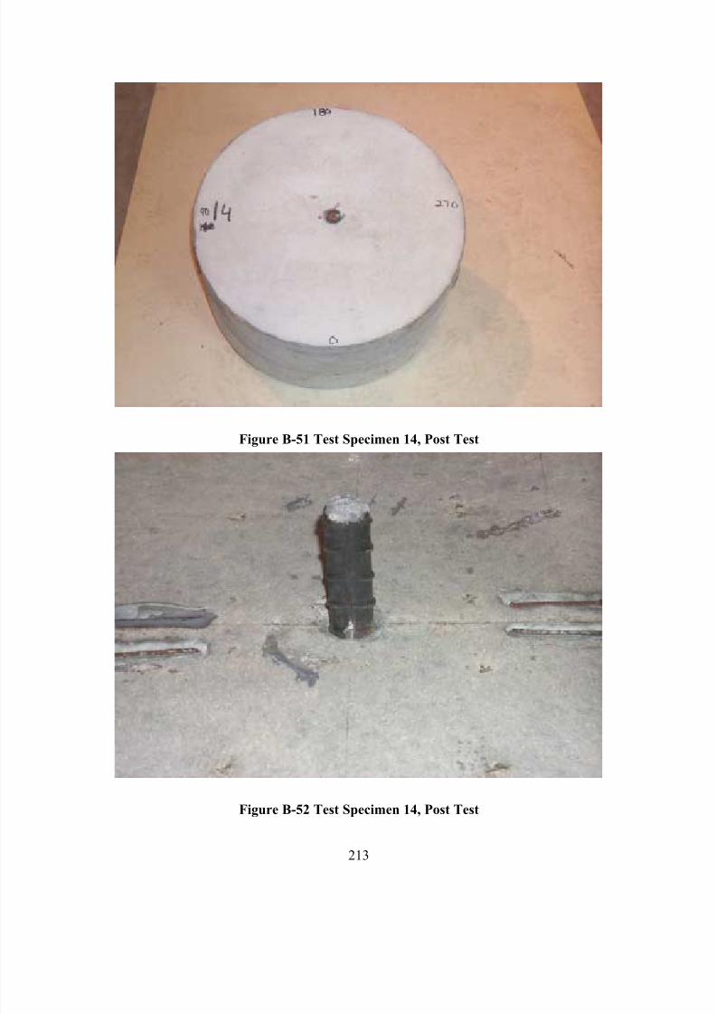
7/28/2019 Weathersby Dis
http://slidepdf.com/reader/full/weathersby-dis 230/280
213
Figure B-51 Test Specimen 14, Post Test
Figure B-52 Test Specimen 14, Post Test
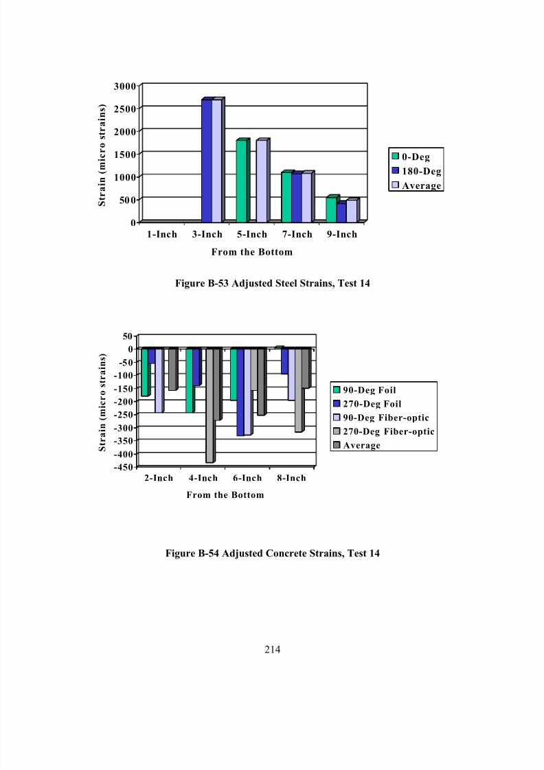
7/28/2019 Weathersby Dis
http://slidepdf.com/reader/full/weathersby-dis 231/280
214
0
500
1000
1500
2000
2500
3000
S t r a i n ( m i c r o s t
r a i n s )
1-Inch 3-Inch 5-Inch 7-Inch 9-Inch
From the Bottom
0-Deg
180-Deg
Average
Figure B-53 Adjusted Steel Strains, Test 14
-450
-400
-350
-300
-250-200
-150
-100
-50
0
50
S t r a i n ( m i c
r o s t r a i n s )
2-Inch 4-Inch 6-Inch 8-Inch
From the Bottom
90-Deg Foil
270-Deg Foil90-Deg Fiber-optic
270-Deg Fiber-optic
Average
Figure B-54 Adjusted Concrete Strains, Test 14
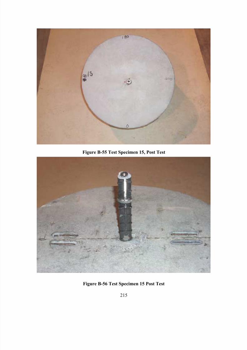
7/28/2019 Weathersby Dis
http://slidepdf.com/reader/full/weathersby-dis 232/280
215
Figure B-55 Test Specimen 15, Post Test
Figure B-56 Test Specimen 15 Post Test
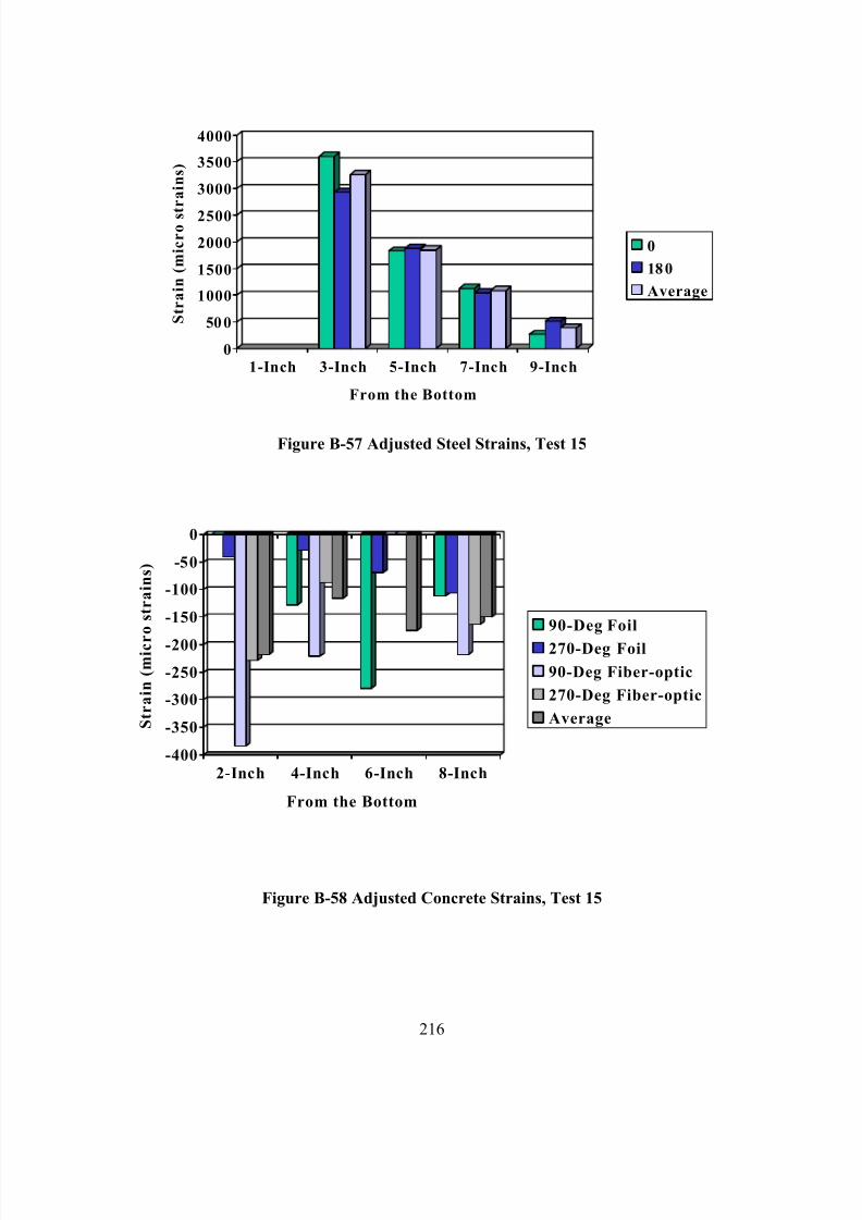
7/28/2019 Weathersby Dis
http://slidepdf.com/reader/full/weathersby-dis 233/280
216
0
500
1000
1500
2000
2500
3000
3500
4000
S t r a i n ( m i c r o s t r a i n s )
1-Inch 3-Inch 5-Inch 7-Inch 9-Inch
From the Bottom
0
180
Average
Figure B-57 Adjusted Steel Strains, Test 15
-400
-350
-300
-250
-200
-150
-100
-50
0
S t r a i n ( m i c r
o s t r a i n s )
2-Inch 4-Inch 6-Inch 8-Inch
From the Bottom
90-Deg Foil
270-Deg Foil
90-Deg Fiber-optic
270-Deg Fiber-optic
Average
Figure B-58 Adjusted Concrete Strains, Test 15
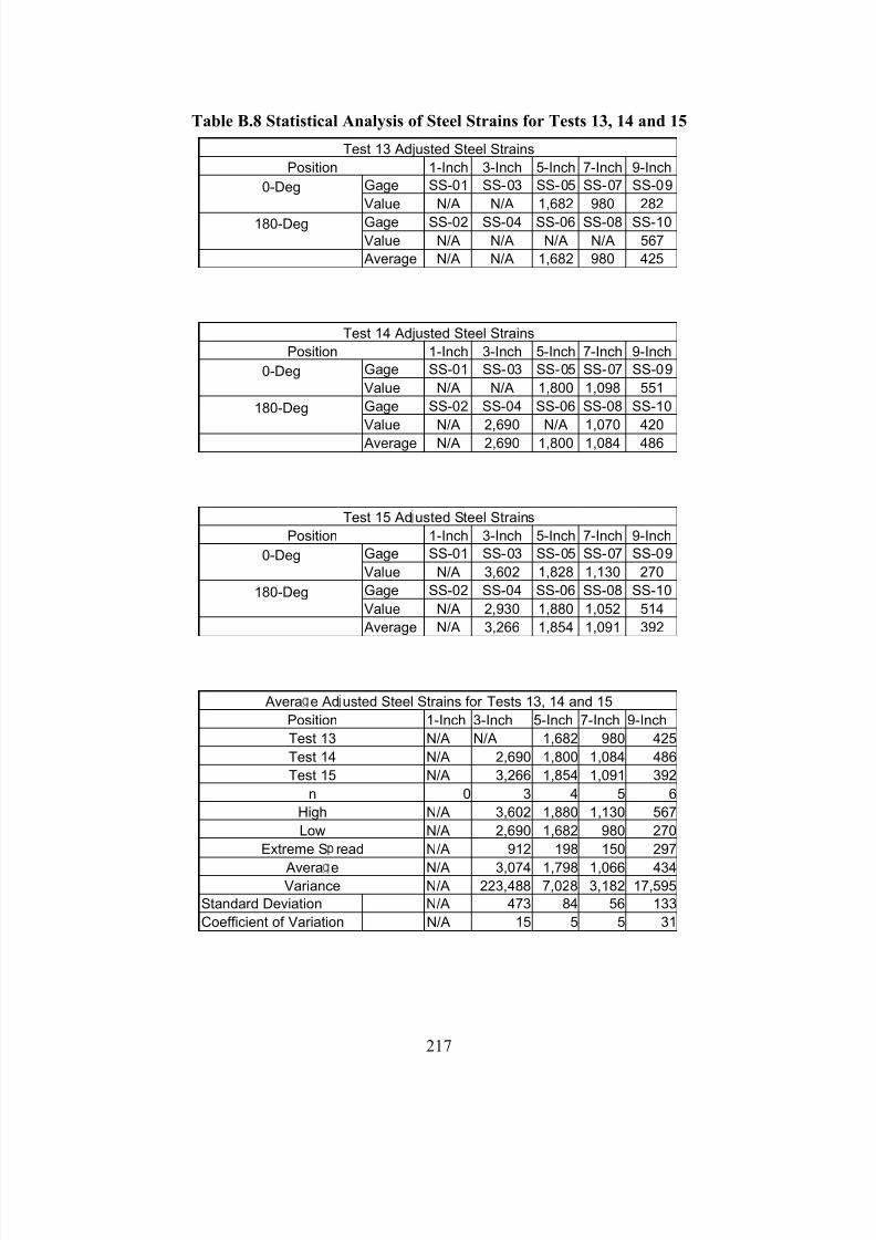
7/28/2019 Weathersby Dis
http://slidepdf.com/reader/full/weathersby-dis 234/280
217
Table B.8 Statistical Analysis of Steel Strains for Tests 13, 14 and 15
Test 13 Adjusted Steel Strains
Position 1-Inch 3-Inch 5-Inch 7-Inch 9-Inch
Gage SS-01 SS-03 SS-05 SS-07 SS-090-Deg
Value N/A N/A 1,682 980 282
Gage SS-02 SS-04 SS-06 SS-08 SS-10180-Deg
Value N/A N/A N/A N/A 567
Average N/A N/A 1,682 980 425
Test 14 Adjusted Steel Strains
Position 1-Inch 3-Inch 5-Inch 7-Inch 9-Inch
Gage SS-01 SS-03 SS-05 SS-07 SS-090-Deg
Value N/A N/A 1,800 1,098 551
Gage SS-02 SS-04 SS-06 SS-08 SS-10180-Deg
Value N/A 2,690 N/A 1,070 420
Average N/A 2,690 1,800 1,084 486
Test 15 Ad usted Steel Strains
Position 1-Inch 3-Inch 5-Inch 7-Inch 9-Inch
Gage SS-01 SS-03 SS-05 SS-07 SS-090-Deg
Value N/A 3,602 1,828 1,130 270
Gage SS-02 SS-04 SS-06 SS-08 SS-10180-Deg
Value N/A 2,930 1,880 1,052 514
Average N/A 3,266 1,854 1,091 392
Avera e Ad usted Steel Strains for Tests 13, 14 and 15
Position 1-Inch 3-Inch 5-Inch 7-Inch 9-Inch
Test 13 N/A N/A 1,682 980 425
Test 14 N/A 2,690 1,800 1,084 486
Test 15 N/A 3,266 1,854 1,091 392
n 0 3 4 5 6
High N/A 3,602 1,880 1,130 567
Low N/A 2,690 1,682 980 270
Extreme S read N/A 912 198 150 297
Avera e N/A 3,074 1,798 1,066 434Variance N/A 223,488 7,028 3,182 17,595
Standard Deviation N/A 473 84 56 133
Coefficient of Variation N/A 15 5 5 31
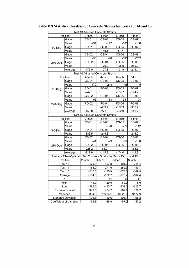
7/28/2019 Weathersby Dis
http://slidepdf.com/reader/full/weathersby-dis 235/280
218
Table B.9 Statistical Analysis of Concrete Strains for Tests 13, 14 and 15
Test 13 Adjusted Concrete Strains
Position 2-Inch 4-Inch 6-Inch 8-Inch
Gage CS-01 CS-03 CS-05 CS-07
Value -294 -147 -105 -106
Gage FO-01 FO-03 FO-05 FO-0790-DegValue -146.3 -87.7
Gage CS-02 CS-04 CS-06 CS-08
Value -56 -48 -106 -257
Gage FO-02 FO-04 FO-06 FO-08270-DegValue -170.0 -108.9 -280.2
Average -175.0 -127.8 -101.9 -214.4
Test 14 Ad usted Concrete Strains
Position 2-Inch 4-Inch 6-Inch 8-Inch
Gage CS-01 CS-03 CS-05 CS-07
Value -179 -243 -195 5
Gage FO-01 FO-03 FO-05 FO-0790-DegValue -242.1 -327.7 -194.2
Gage CS-02 CS-04 CS-06 CS-08
Value -53 -138 -331 -94
Gage FO-02 FO-04 FO-06 FO-08270-DegValue -433.7 -157.9 -315.7
Average -158.0 -271.6 -252.9 -149.7
Test 15 Adjusted Concrete Strains
Position 2-Inch 4-Inch 6-Inch 8-Inch
Gage CS-01 CS-03 CS-05 CS-07
Value -128 -279 -112
Gage FO-01 FO-03 FO-05 FO-0790-DegValue -383.5 -219.8 -218.2
Gage CS-02 CS-04 CS-06 CS-08
Value -41 -29 -69 -106Gage FO-02 FO-04 FO-06 FO-08270-DegValue -228.2 -86.7 -163.5
Average -217.6 -115.9 -174.0 -149.9
Average Fiber-Optic and Foil Concrete Strains for Tests 13, 14 and 15
Position 2-Inch 4-Inch 6-Inch 8-Inch
Test 13 -175.0 -127.8 -101.9 -214.4
Test 14 -158.0 -271.6 -252.9 -149.7
Test 15 -217.6 -115.9 -174.0 -149.9
Average -184.6 -162.7 -176.7 -167.4
n 8 11 10 11
High -41.0 -29.0 -69.0 5.0
Low -383.5 -433.7 -331.0 -3
15.7Extreme Spread 342.5 404.7 262.0 320.7
Variance 15894.0 12234.1 10226.6 9177.9
Standard Deviation 126.1 110.6 101.1 95.8
Coefficient of Variation -68.3 -68.0 -57.2 -57.2
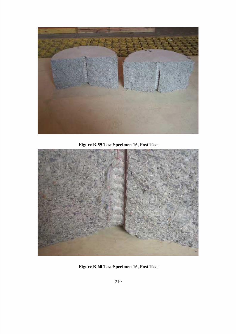
7/28/2019 Weathersby Dis
http://slidepdf.com/reader/full/weathersby-dis 236/280
219
Figure B-59 Test Specimen 16, Post Test
Figure B-60 Test Specimen 16, Post Test
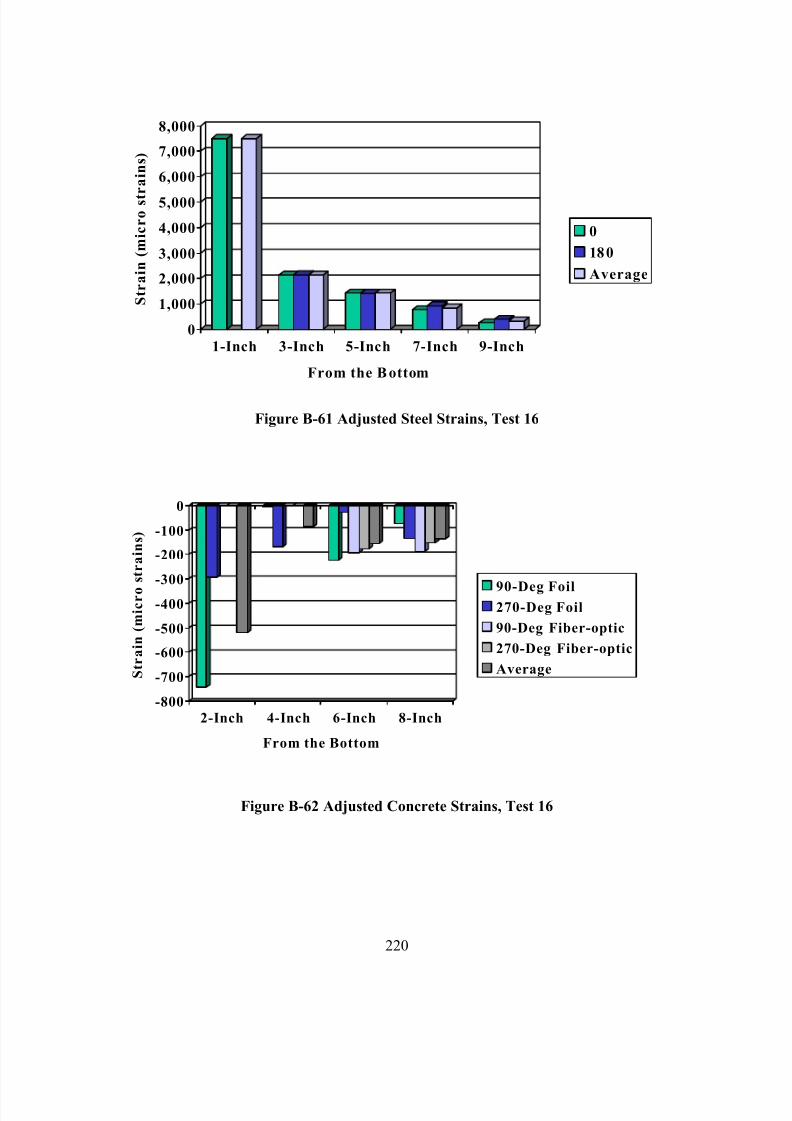
7/28/2019 Weathersby Dis
http://slidepdf.com/reader/full/weathersby-dis 237/280
220
0
1,000
2,000
3,000
4,000
5,000
6,000
7,000
8,000
S t r a i n ( m i c r o s t r a i n s )
1-Inch 3-Inch 5-Inch 7-Inch 9-Inch
From the Bottom
0
180
Average
Figure B-61 Adjusted Steel Strains, Test 16
-800
-700
-600
-500
-400
-300
-200
-100
0
S t r a i n ( m i c r o
s t r a i n s )
2-Inch 4-Inch 6-Inch 8-Inch
From the Bottom
90-Deg Foil270-Deg Foil
90-Deg Fiber-optic
270-Deg Fiber-optic
Average
Figure B-62 Adjusted Concrete Strains, Test 16
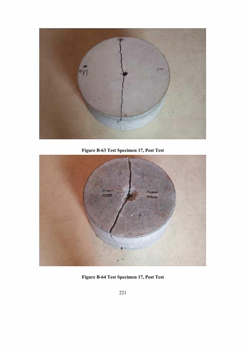
7/28/2019 Weathersby Dis
http://slidepdf.com/reader/full/weathersby-dis 238/280
221
Figure B-63 Test Specimen 17, Post Test
Figure B-64 Test Specimen 17, Post Test
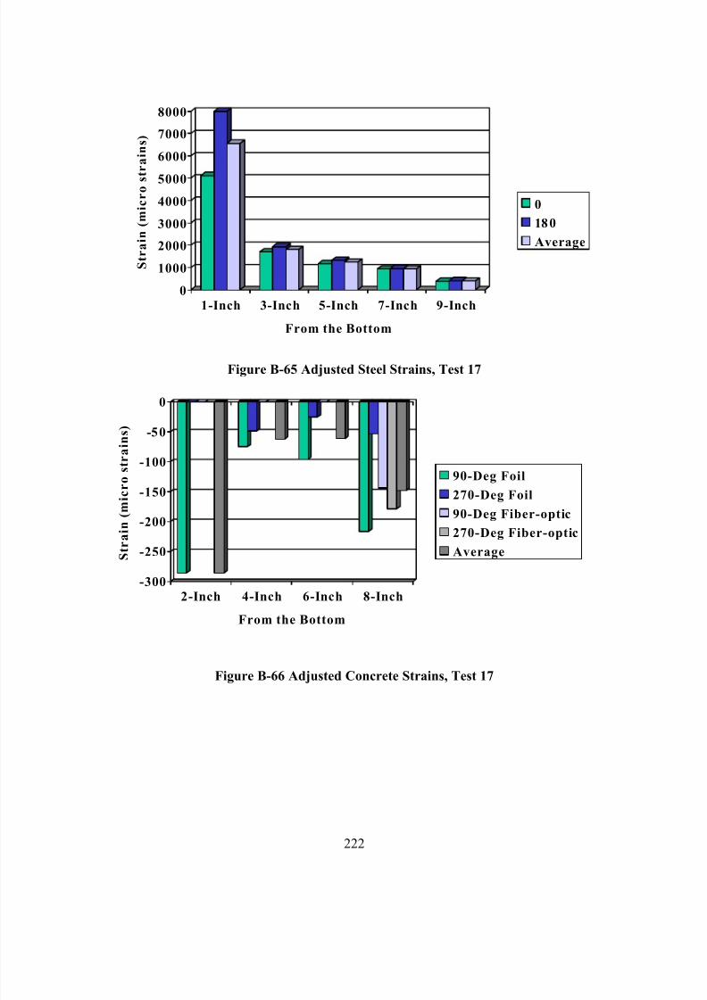
7/28/2019 Weathersby Dis
http://slidepdf.com/reader/full/weathersby-dis 239/280
222
0
1000
2000
3000
4000
5000
6000
7000
8000
S t r a i n ( m i c r o s t
r a i n s )
1-Inch 3-Inch 5-Inch 7-Inch 9-Inch
From the Bottom
0
180
Average
Figure B-65 Adjusted Steel Strains, Test 17
-300
-250
-200
-150
-100
-50
0
S t r a i n
( m i c r o s t r a i n s )
2-Inch 4-Inch 6-Inch 8-Inch
From the Bottom
90-Deg Foil
270-Deg Foil
90-Deg Fiber-optic
270-Deg Fiber-optic
Average
Figure B-66 Adjusted Concrete Strains, Test 17
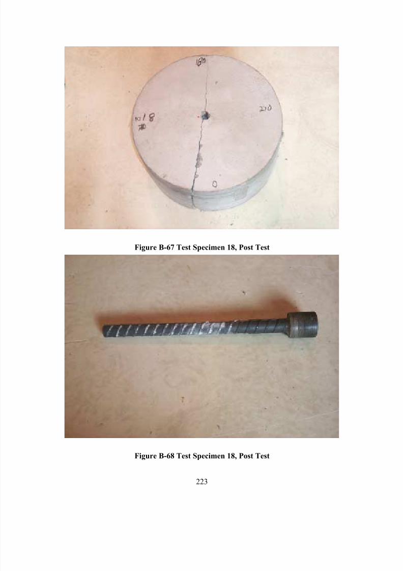
7/28/2019 Weathersby Dis
http://slidepdf.com/reader/full/weathersby-dis 240/280
223
Figure B-67 Test Specimen 18, Post Test
Figure B-68 Test Specimen 18, Post Test
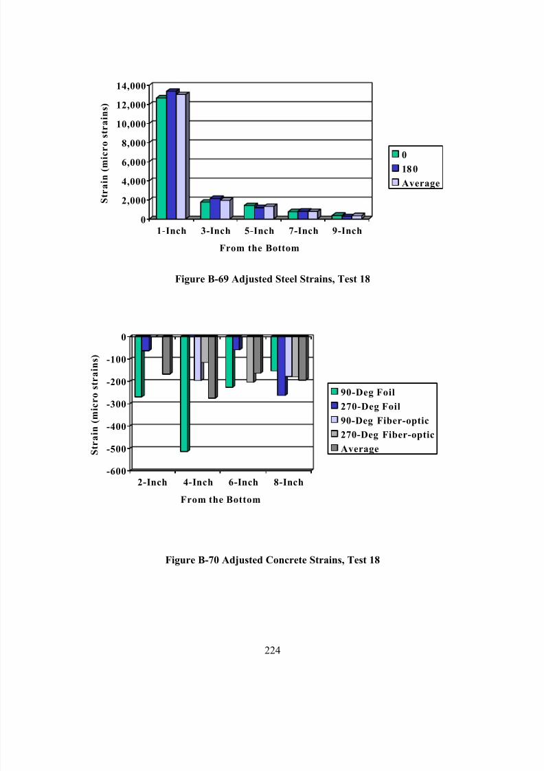
7/28/2019 Weathersby Dis
http://slidepdf.com/reader/full/weathersby-dis 241/280
224
0
2,000
4,000
6,000
8,000
10,000
12,000
14,000
S t r a i n ( m i c r o s t r a i n s )
1-Inch 3-Inch 5-Inch 7-Inch 9-Inch
From the Bottom
0
180
Average
Figure B-69 Adjusted Steel Strains, Test 18
-600
-500
-400
-300
-200
-100
0
S t r a i n ( m i c
r o s t r a i n s )
2-Inch 4-Inch 6-Inch 8-Inch
From the Bottom
90-Deg Foil
270-Deg Foil
90-Deg Fiber-optic
270-Deg Fiber-optic
Average
Figure B-70 Adjusted Concrete Strains, Test 18
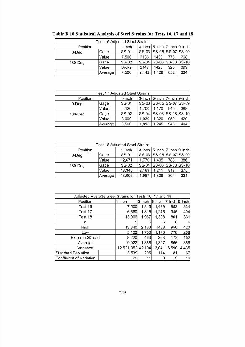
7/28/2019 Weathersby Dis
http://slidepdf.com/reader/full/weathersby-dis 242/280
225
Table B.10 Statistical Analysis of Steel Strains for Tests 16, 17 and 18
Test 16 Adjusted Steel Strains
Position 1-Inch 3-Inch 5-Inch 7-Inch 9-Inch
Gage SS-01 SS-03 SS-05 SS-07 SS-090-Deg
Value 7,500 2136 1438 778 268
Gage SS-02 SS-04 SS-06 SS-08 SS-10180-Deg
Value Broke 2147 1420 925 399
Average 7,500 2,142 1,429 852 334
Test 17 Adjusted Steel Strains
Position 1-Inch 3-Inch 5-Inch 7-Inch 9-Inch
Gage SS-01 SS-03 SS-05 SS-07 SS-090-Deg
Value 5,120 1,700 1,170 940 388
Gage SS-02 SS-04 SS-06 SS-08 SS-10180-Deg
Value 8,000 1,930 1,320 950 420
Average 6,560 1,815 1,245 945 404
Test 18 Ad usted Steel Strains
Position 1-Inch 3-Inch 5-Inch 7-Inch 9-Inch
Gage SS-01 SS-03 SS-05 SS-07 SS-090-Deg
Value 12,671 1,770 1,405 783 386
Gage SS-02 SS-04 SS-06 SS-08 SS-10180-Deg
Value 13,340 2,163 1,211 818 275
Average 13,006 1,967 1,308 801 331
Ad usted Avera e Steel Strains for Tests 16, 17 and 18
Position 1-Inch 3-Inch 5-Inch 7-Inch 9-Inch
Test 16 7,500 1,815 1,429 852 334
Test 17 6,560 1,815 1,245 945 404
Test 18 13,006 1,967 1,308 801 331
n 5 6 6 6 6
High 13,340 2,163 1438 950 420
Low 5,120 1,700 1,170 778 268
Extreme S read 8,220 463 268 172 152
Avera e 9,022 1,866 1,327 866 356Variance 12,521,052 42,104 13,041 6,590 4,435
Standard Deviation 3,539 205 114 81 67
Coefficient of Variation 39 11 9 9 19
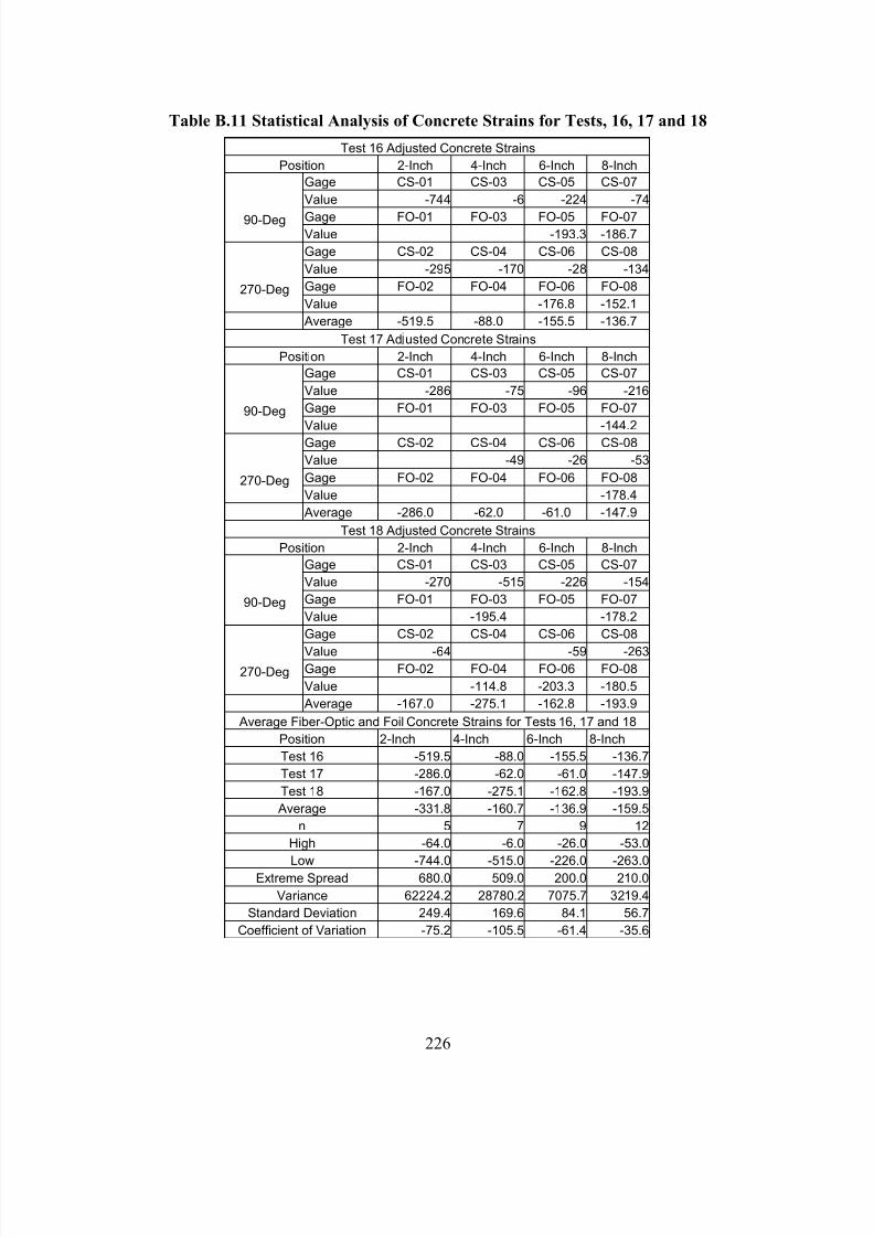
7/28/2019 Weathersby Dis
http://slidepdf.com/reader/full/weathersby-dis 243/280
226
Table B.11 Statistical Analysis of Concrete Strains for Tests, 16, 17 and 18
Test 16 Adjusted Concrete Strains
Position 2-Inch 4-Inch 6-Inch 8-Inch
Gage CS-01 CS-03 CS-05 CS-07
Value -744 -6 -224 -74
Gage FO-01 FO-03 FO-05 FO-0790-DegValue -193.3 -186.7
Gage CS-02 CS-04 CS-06 CS-08
Value -295 -170 -28 -134
Gage FO-02 FO-04 FO-06 FO-08270-DegValue -176.8 -152.1
Average -519.5 -88.0 -155.5 -136.7
Test 17 Ad usted Concrete Strains
Position 2-Inch 4-Inch 6-Inch 8-Inch
Gage CS-01 CS-03 CS-05 CS-07
Value -286 -75 -96 -216
Gage FO-01 FO-03 FO-05 FO-0790-DegValue -144.2
Gage CS-02 CS-04 CS-06 CS-08
Value -49 -26 -53
Gage FO-02 FO-04 FO-06 FO-08270-DegValue -178.4
Average -286.0 -62.0 -61.0 -147.9
Test 18 Adjusted Concrete Strains
Position 2-Inch 4-Inch 6-Inch 8-Inch
Gage CS-01 CS-03 CS-05 CS-07
Value -270 -515 -226 -154
Gage FO-01 FO-03 FO-05 FO-0790-DegValue -195.4 -178.2
Gage CS-02 CS-04 CS-06 CS-08
Value -64 -59 -263Gage FO-02 FO-04 FO-06 FO-08270-DegValue -114.8 -203.3 -180.5
Average -167.0 -275.1 -162.8 -193.9
Average Fiber-Optic and Foil Concrete Strains for Tests 16, 17 and 18
Position 2-Inch 4-Inch 6-Inch 8-Inch
Test 16 -519.5 -88.0 -155.5 -136.7
Test 17 -286.0 -62.0 -61.0 -147.9
Test 18 -167.0 -275.1 -162.8 -193.9
Average -331.8 -160.7 -136.9 -159.5
n 5 7 9 12
High -64.0 -6.0 -26.0 -53.0
Low -744.0 -515.0 -226.0 -263.0Extreme Spread 680.0 509.0 200.0 210.0
Variance 62224.2 28780.2 7075.7 3219.4
Standard Deviation 249.4 169.6 84.1 56.7
Coefficient of Variation -75.2 -105.5 -61.4 -35.6
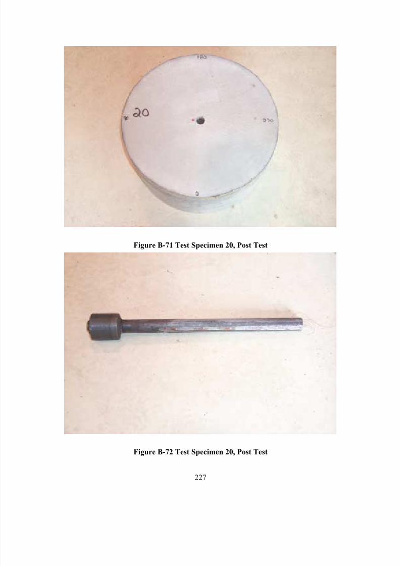
7/28/2019 Weathersby Dis
http://slidepdf.com/reader/full/weathersby-dis 244/280
227
Figure B-71 Test Specimen 20, Post Test
Figure B-72 Test Specimen 20, Post Test
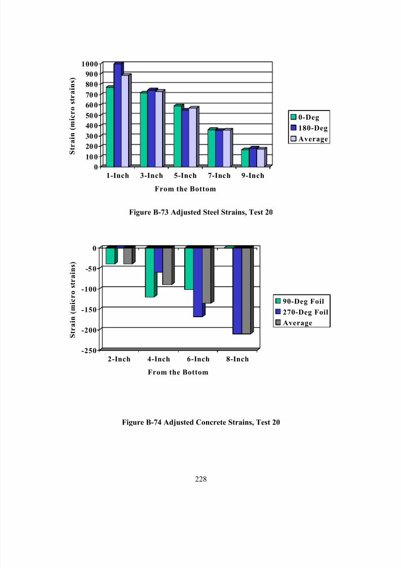
7/28/2019 Weathersby Dis
http://slidepdf.com/reader/full/weathersby-dis 245/280
228
0
100
200
300
400
500
600
700
800
900
1000
S t r a i n ( m i c r o s t r a i n s )
1-Inch 3-Inch 5-Inch 7-Inch 9-Inch
From the Bottom
0-Deg
180-Deg
Average
Figure B-73 Adjusted Steel Strains, Test 20
-250
-200
-150
-100
-50
0
S t r a i n ( m i c r o s t r a i n s )
2-Inch 4-Inch 6-Inch 8-Inch
From the Bottom
90-Deg Foil
270-Deg Foil
Average
Figure B-74 Adjusted Concrete Strains, Test 20
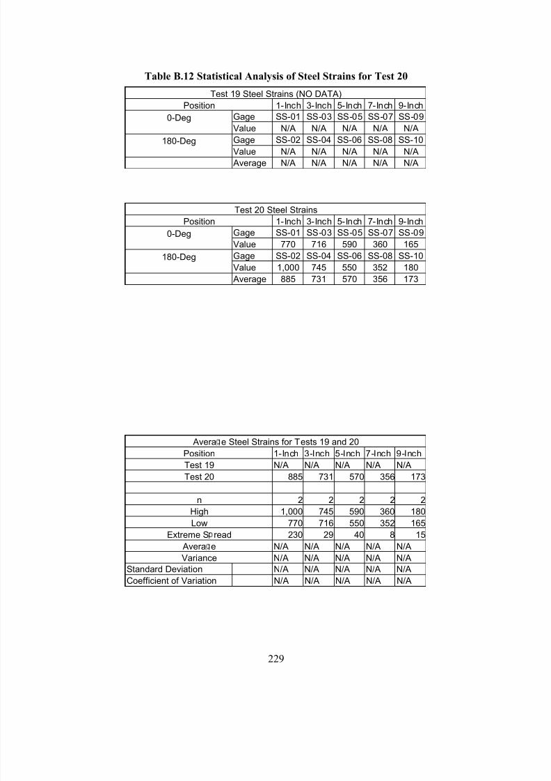
7/28/2019 Weathersby Dis
http://slidepdf.com/reader/full/weathersby-dis 246/280
229
Table B.12 Statistical Analysis of Steel Strains for Test 20
Test 19 Steel Strains (NO DATA)
Position 1-Inch 3-Inch 5-Inch 7-Inch 9-Inch
Gage SS-01 SS-03 SS-05 SS-07 SS-090-Deg
Value N/A N/A N/A N/A N/A
Gage SS-02 SS-04 SS-06 SS-08 SS-10180-Deg
Value N/A N/A N/A N/A N/A
Average N/A N/A N/A N/A N/A
Test 20 Steel Strains
Position 1-Inch 3-Inch 5-Inch 7-Inch 9-Inch
Gage SS-01 SS-03 SS-05 SS-07 SS-090-Deg
Value 770 716 590 360 165
Gage SS-02 SS-04 SS-06 SS-08 SS-10180-Deg
Value 1,000 745 550 352 180
Average 885 731 570 356 173
Avera e Steel Strains for Tests 19 and 20
Position 1-Inch 3-Inch 5-Inch 7-Inch 9-Inch
Test 19 N/A N/A N/A N/A N/A
Test 20 885 731 570 356 173
n 2 2 2 2 2
High 1,000 745 590 360 180
Low 770 716 550 352 165
Extreme S read 230 29 40 8 15
Avera e N/A N/A N/A N/A N/AVariance N/A N/A N/A N/A N/A
Standard Deviation N/A N/A N/A N/A N/A
Coefficient of Variation N/A N/A N/A N/A N/A
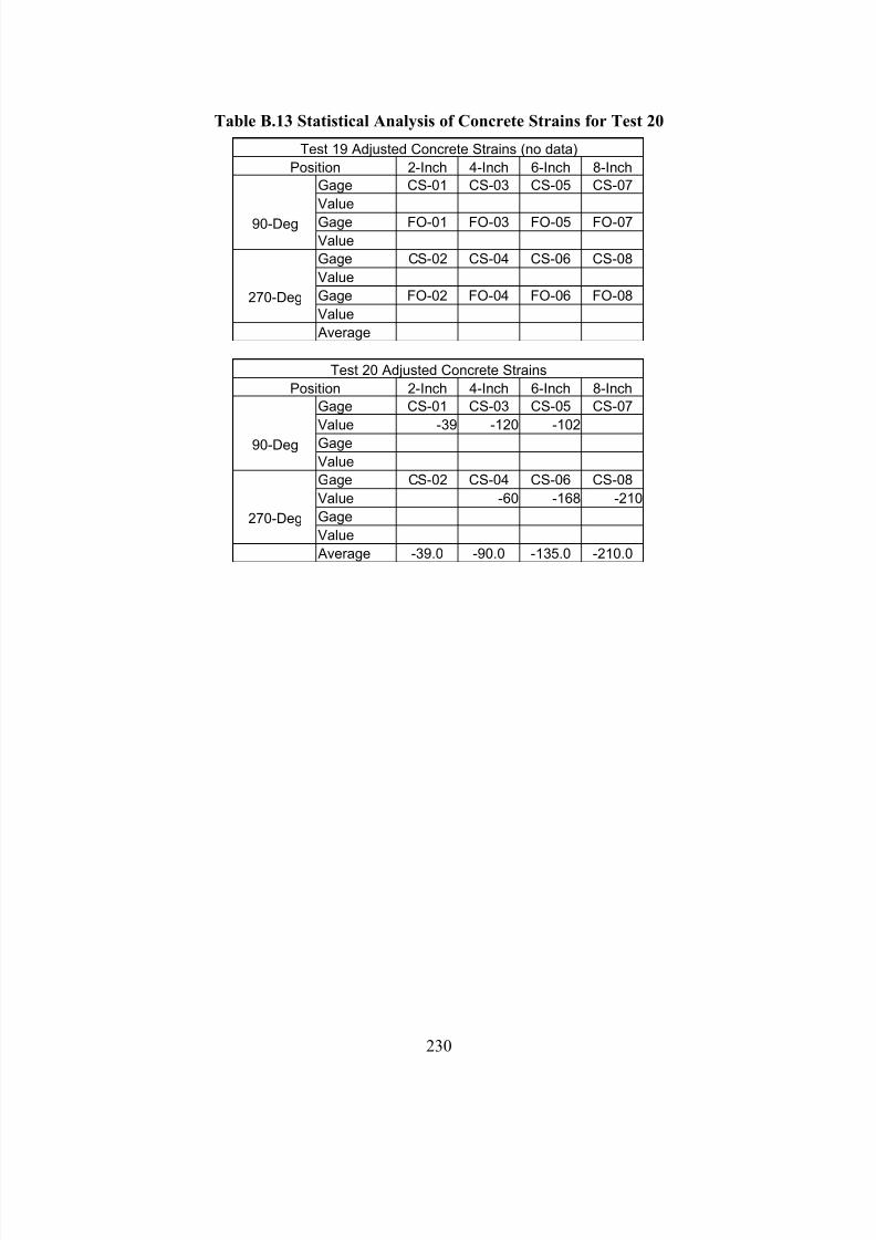
7/28/2019 Weathersby Dis
http://slidepdf.com/reader/full/weathersby-dis 247/280
230
Table B.13 Statistical Analysis of Concrete Strains for Test 20
Test 19 Adjusted Concrete Strains (no data)
Position 2-Inch 4-Inch 6-Inch 8-Inch
Gage CS-01 CS-03 CS-05 CS-07
Value
Gage FO-01 FO-03 FO-05 FO-0790-Deg
Value
Gage CS-02 CS-04 CS-06 CS-08
Value
Gage FO-02 FO-04 FO-06 FO-08270-Deg
Value
Average
Test 20 Adjusted Concrete Strains
Position 2-Inch 4-Inch 6-Inch 8-Inch
Gage CS-01 CS-03 CS-05 CS-07
Value -39 -120 -102
Gage90-Deg
Value
Gage CS-02 CS-04 CS-06 CS-08
Value -60 -168 -210
Gage270-Deg
Value
Average -39.0 -90.0 -135.0 -210.0
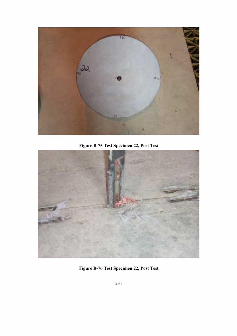
7/28/2019 Weathersby Dis
http://slidepdf.com/reader/full/weathersby-dis 248/280
231
Figure B-75 Test Specimen 22, Post Test
Figure B-76 Test Specimen 22, Post Test
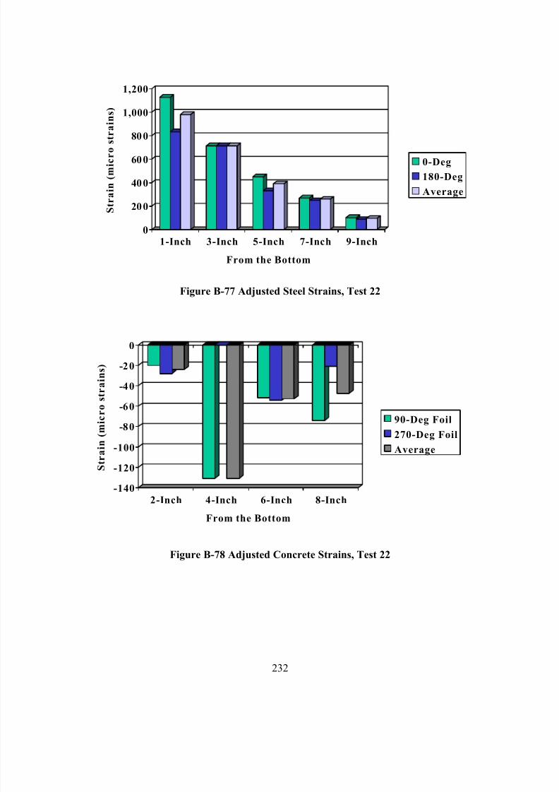
7/28/2019 Weathersby Dis
http://slidepdf.com/reader/full/weathersby-dis 249/280
232
0
200
400
600
800
1,000
1,200
S t r a i n ( m i c r o s t
r a i n s )
1-Inch 3-Inch 5-Inch 7-Inch 9-Inch
From the Bottom
0-Deg
180-Deg
Average
Figure B-77 Adjusted Steel Strains, Test 22
-140
-120
-100
-80
-60
-40
-20
0
S t r a i n ( m i c r o s t r a i n s )
2-Inch 4-Inch 6-Inch 8-Inch
From the Bottom
90-Deg Foil
270-Deg Foil
Average
Figure B-78 Adjusted Concrete Strains, Test 22
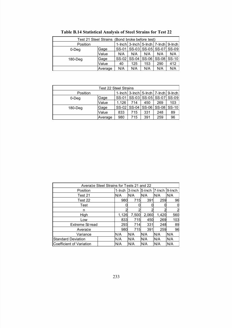
7/28/2019 Weathersby Dis
http://slidepdf.com/reader/full/weathersby-dis 250/280
233
Table B.14 Statistical Analysis of Steel Strains for Test 22
Test 21 Steel Strains (Bond broke before test)
Position 1-Inch 3-Inch 5-Inch 7-Inch 9-Inch
Gage SS-01 SS-03 SS-05 SS-07 SS-090-Deg
Value N/A N/A N/A N/A N/A
Gage SS-02 SS-04 SS-06 SS-08 SS-10180-Deg
Value 40 125 153 290 412
Average N/A N/A N/A N/A N/A
Test 22 Steel Strains
Position 1-Inch 3-Inch 5-Inch 7-Inch 9-Inch
Gage SS-01 SS-03 SS-05 SS-07 SS-090-Deg
Value 1,126 714 450 269 103
Gage SS-02 SS-04 SS-06 SS-08 SS-10180-Deg
Value 833 715 331 248 89
Average 980 715 391 259 96
Avera e Steel Strains for Tests 21 and 22
Position 1-Inch 3-Inch 5-Inch 7-Inch 9-Inch
Test 21 N/A N/A N/A N/A N/A
Test 22 980 715 391 259 96
Test 0 0 0 0 0
n 2 2 2 2 2
High 1,126 7,500 2,060 1,420 560
Low 833 715 450 269 103
Extreme S read 293 714 331 248 89
Avera e 980 715 391 259 96Variance N/A N/A N/A N/A N/A
Standard Deviation N/A N/A N/A N/A N/A
Coefficient of Variation N/A N/A N/A N/A N/A
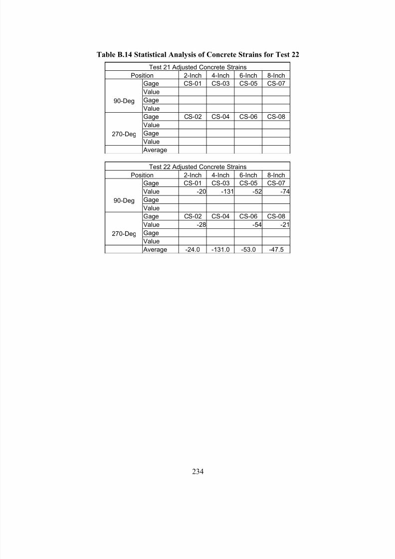
7/28/2019 Weathersby Dis
http://slidepdf.com/reader/full/weathersby-dis 251/280
234
Table B.14 Statistical Analysis of Concrete Strains for Test 22
Test 21 Adjusted Concrete Strains
Position 2-Inch 4-Inch 6-Inch 8-Inch
Gage CS-01 CS-03 CS-05 CS-07
Value
Gage90-Deg
Value
Gage CS-02 CS-04 CS-06 CS-08
Value
Gage270-Deg
Value
Average
Test 22 Adjusted Concrete Strains
Position 2-Inch 4-Inch 6-Inch 8-Inch
Gage CS-01 CS-03 CS-05 CS-07
Value -20 -131 -52 -74
Gage90-Deg
Value
Gage CS-02 CS-04 CS-06 CS-08
Value -28 -54 -21
Gage270-Deg
Value
Average -24.0 -131.0 -53.0 -47.5
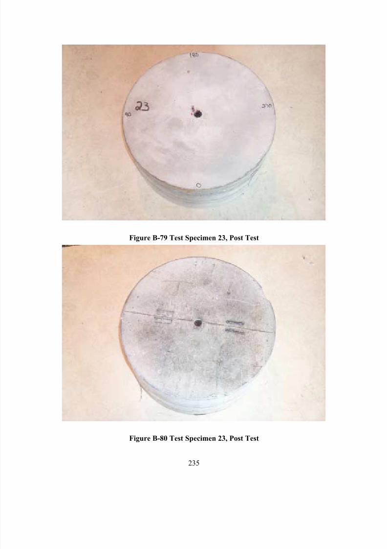
7/28/2019 Weathersby Dis
http://slidepdf.com/reader/full/weathersby-dis 252/280
235
Figure B-79 Test Specimen 23, Post Test
Figure B-80 Test Specimen 23, Post Test
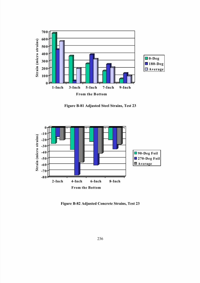
7/28/2019 Weathersby Dis
http://slidepdf.com/reader/full/weathersby-dis 253/280
236
0
100
200
300
400
500
600
700
S t r a i n ( m i c r o s t r a i n s )
1-Inch 3-Inch 5-Inch 7-Inch 9-Inch
From the Bottom
0-Deg
180-Deg
Average
Figure B-81 Adjusted Steel Strains, Test 23
-80
-70
-60
-50
-40
-30
-20
-10
0
S t r a i n ( m i c r o
s t r a i n s )
2-Inch 4-Inch 6-Inch 8-Inch
From the Bottom
90-Deg Foil
270-Deg Foil
Average
Figure B-82 Adjusted Concrete Strains, Test 23
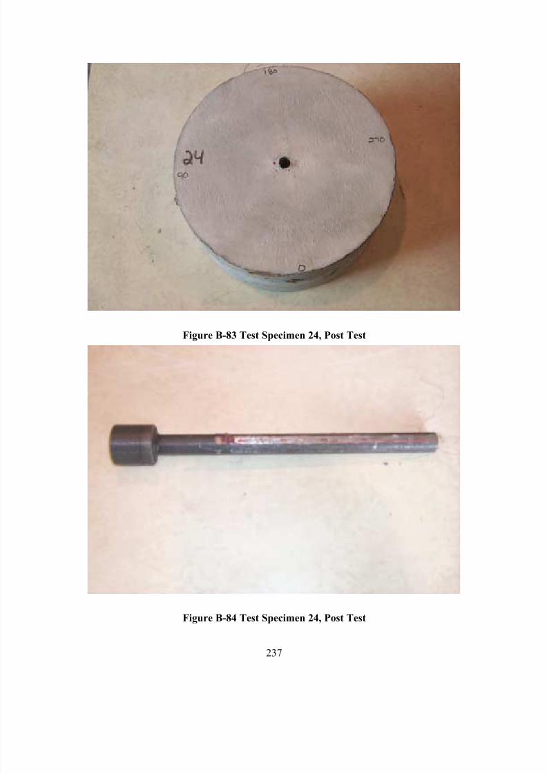
7/28/2019 Weathersby Dis
http://slidepdf.com/reader/full/weathersby-dis 254/280
237
Figure B-83 Test Specimen 24, Post Test
Figure B-84 Test Specimen 24, Post Test
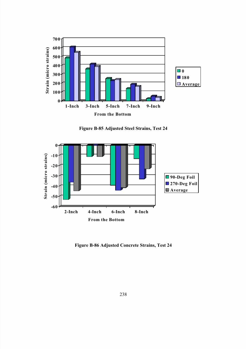
7/28/2019 Weathersby Dis
http://slidepdf.com/reader/full/weathersby-dis 255/280
238
0
100
200
300
400
500
600
700
S t r a i n ( m i c r o s t
r a i n s )
1-Inch 3-Inch 5-Inch 7-Inch 9-Inch
From the Bottom
0
180
Average
Figure B-85 Adjusted Steel Strains, Test 24
-60
-50
-40
-30
-20
-10
0
S t r a i n ( m i c r o s t r a i n s )
2-Inch 4-Inch 6-Inch 8-Inch
From the Bottom
90-Deg Foil
270-Deg FoilAverage
Figure B-86 Adjusted Concrete Strains, Test 24

7/28/2019 Weathersby Dis
http://slidepdf.com/reader/full/weathersby-dis 256/280
239
Table B.15 Statistical Analysis of Steel Strains for Tests 23 and 24
Test 23 Adjusted Steel Strains
Position 1-Inch 3-Inch 5-Inch 7-Inch 9-Inch
Gage SS-01 SS-03 SS-05 SS-07 SS-090-Deg
Value 681 369 265 167 60
Gage SS-02 SS-04 SS-06 SS-08 SS-10180-Deg
Value 458 N/A 388 257 135
Average 570 369 327 212 98
Test 24 Adjusted Steel Strains
Position 1-Inch 3-Inch 5-Inch 7-Inch 9-Inch
Gage SS-01 SS-03 SS-05 SS-07 SS-090-Deg
Value 485 360 252 138 25
Gage SS-02 SS-04 SS-06 SS-08 SS-10180-Deg
Value 608 415 229 187 54
Average 547 388 241 163 40
Avera e Ad usted Steel Strains for Tests 23 and 24
Position 1-Inch 3-Inch 5-Inch 7-Inch 9-Inch
Test 23 570 369 327 212 98
Test 24 547 388 241 163 40
n 4 3 4 4 4
High 681 415 388 257 135
Low 458 360 229 138 25
Extreme S read 223 55 159 119 110
Avera e 558 381 284 187 69Variance 10,986 870 5,075 2,567 2,199
Standard Deviation 105 30 71 51 47
Coefficient of Variation 19 8 25 27 68
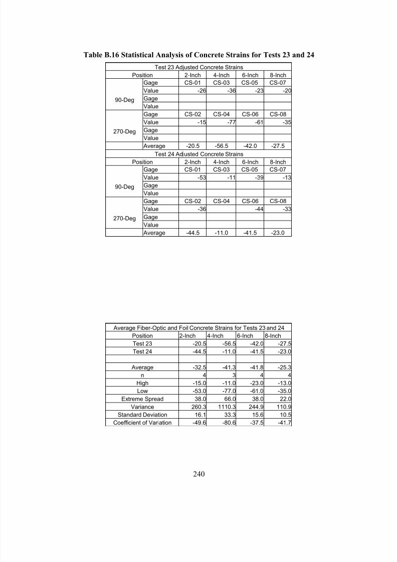
7/28/2019 Weathersby Dis
http://slidepdf.com/reader/full/weathersby-dis 257/280
240
Table B.16 Statistical Analysis of Concrete Strains for Tests 23 and 24
Test 23 Adjusted Concrete Strains
Position 2-Inch 4-Inch 6-Inch 8-Inch
Gage CS-01 CS-03 CS-05 CS-07
Value -26 -36 -23 -20
Gage90-DegValue
Gage CS-02 CS-04 CS-06 CS-08
Value -15 -77 -61 -35
Gage270-DegValue
Average -20.5 -56.5 -42.0 -27.5
Test 24 Ad usted Concrete Strains
Position 2-Inch 4-Inch 6-Inch 8-Inch
Gage CS-01 CS-03 CS-05 CS-07
Value -53 -11 -39 -13
Gage90-DegValue
Gage CS-02 CS-04 CS-06 CS-08
Value -36 -44 -33
Gage270-DegValue
Average -44.5 -11.0 -41.5 -23.0
Average Fiber-Optic and Foil Concrete Strains for Tests 23 and 24
Position 2-Inch 4-Inch 6-Inch 8-Inch
Test 23 -20.5 -56.5 -42.0 -27.5
Test 24 -44.5 -11.0 -41.5 -23.0
Average -32.5 -41.3 -41.8 -25.3
n 4 3 4 4
High -15.0 -11.0 -23.0 -13.0
Low -53.0 -77.0 -61.0 -35.0Extreme Spread 38.0 66.0 38.0 22.0
Variance 260.3 1110.3 244.9 110.9
Standard Deviation 16.1 33.3 15.6 10.5
Coefficient of Variation -49.6 -80.6 -37.5 -41.7
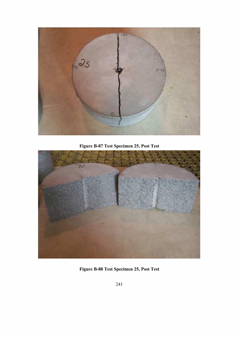
7/28/2019 Weathersby Dis
http://slidepdf.com/reader/full/weathersby-dis 258/280
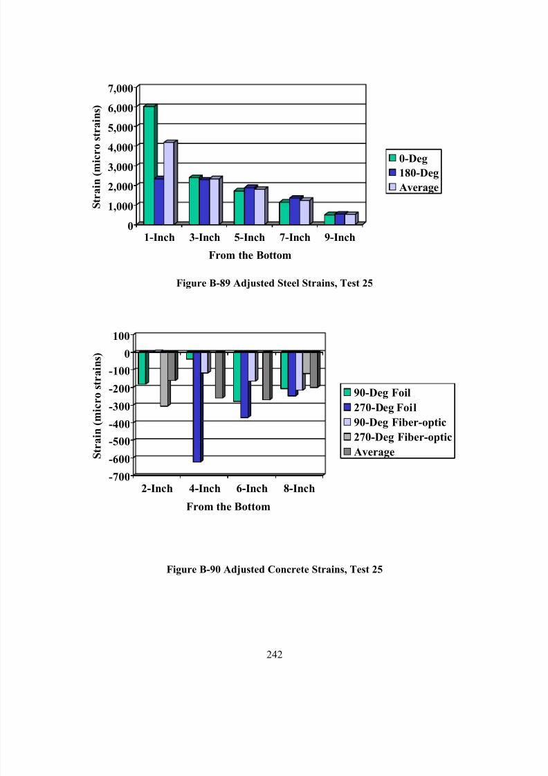
7/28/2019 Weathersby Dis
http://slidepdf.com/reader/full/weathersby-dis 259/280
242
0
1,000
2,000
3,000
4,000
5,000
6,000
7,000
S t r a i n ( m i c r o s t
r a i n s )
1-Inch 3-Inch 5-Inch 7-Inch 9-Inch
From the Bottom
0-Deg
180-Deg
Average
Figure B-89 Adjusted Steel Strains, Test 25
-700
-600
-500
-400-300
-200
-100
0
100
S t r a i n ( m i c
r o s t r a i n s )
2-Inch 4-Inch 6-Inch 8-Inch
From the Bottom
90-Deg Foil
270-Deg Foil90-Deg Fiber-optic
270-Deg Fiber-optic
Average
Figure B-90 Adjusted Concrete Strains, Test 25
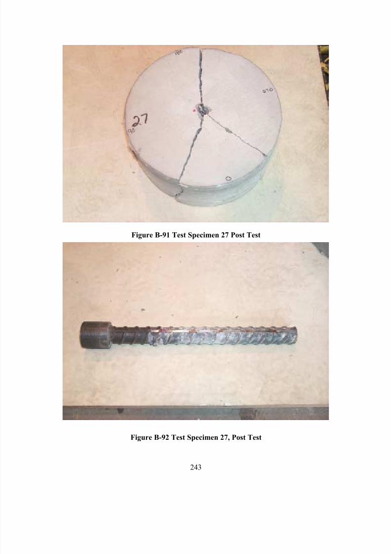
7/28/2019 Weathersby Dis
http://slidepdf.com/reader/full/weathersby-dis 260/280
243
Figure B-91 Test Specimen 27 Post Test
Figure B-92 Test Specimen 27, Post Test
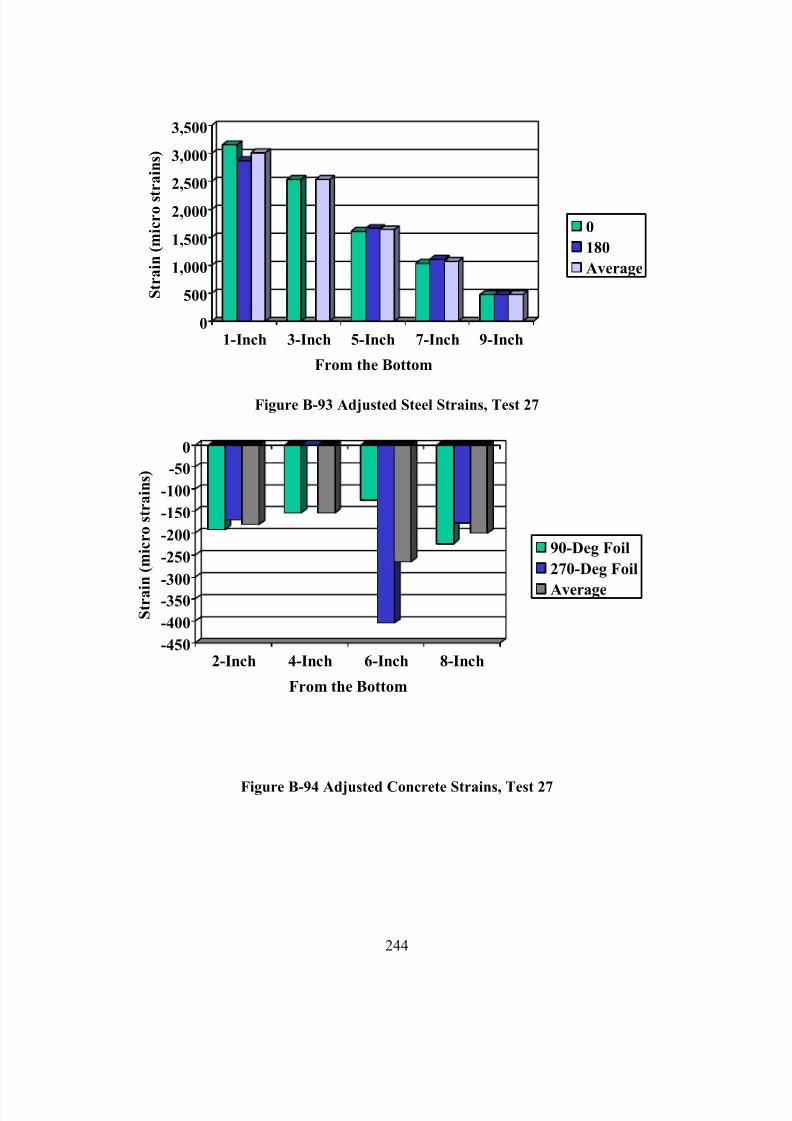
7/28/2019 Weathersby Dis
http://slidepdf.com/reader/full/weathersby-dis 261/280
244
0
500
1,000
1,500
2,000
2,500
3,000
3,500
S t r a i n ( m i c r o s t r a i n s )
1-Inch 3-Inch 5-Inch 7-Inch 9-Inch
From the Bottom
0
180
Average
Figure B-93 Adjusted Steel Strains, Test 27
-450
-400
-350
-300
-250
-200
-150
-100
-50
0
S t r a i
n ( m i c r o s t r a i n s )
2-Inch 4-Inch 6-Inch 8-Inch
From the Bottom
90-Deg Foil
270-Deg Foil
Average
Figure B-94 Adjusted Concrete Strains, Test 27
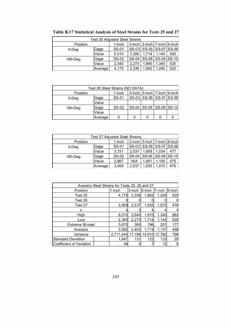
7/28/2019 Weathersby Dis
http://slidepdf.com/reader/full/weathersby-dis 262/280
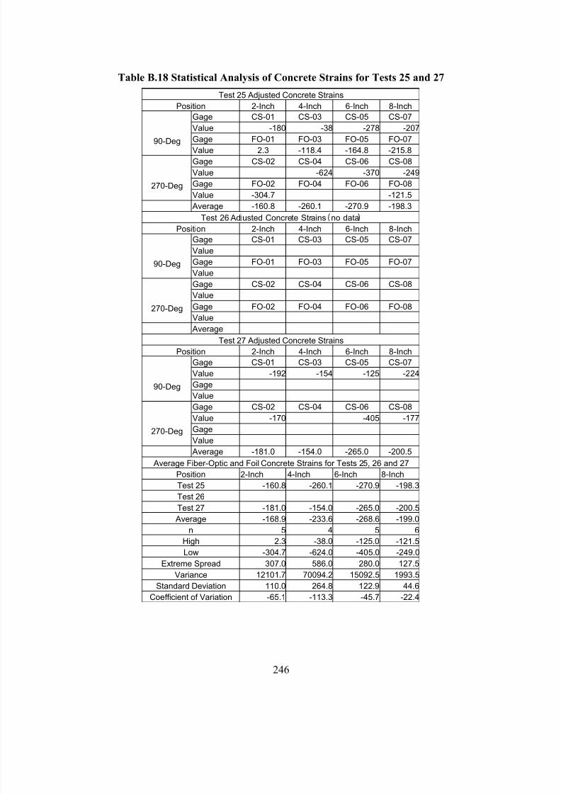
7/28/2019 Weathersby Dis
http://slidepdf.com/reader/full/weathersby-dis 263/280
246
Table B.18 Statistical Analysis of Concrete Strains for Tests 25 and 27
Test 25 Adjusted Concrete Strains
Position 2-Inch 4-Inch 6-Inch 8-Inch
Gage CS-01 CS-03 CS-05 CS-07
Value -180 -38 -278 -207
Gage FO-01 FO-03 FO-05 FO-0790-DegValue 2.3 -118.4 -164.8 -215.8
Gage CS-02 CS-04 CS-06 CS-08
Value -624 -370 -249
Gage FO-02 FO-04 FO-06 FO-08270-DegValue -304.7 -121.5
Average -160.8 -260.1 -270.9 -198.3
Test 26 Ad usted Concrete Strains no data
Position 2-Inch 4-Inch 6-Inch 8-Inch
Gage CS-01 CS-03 CS-05 CS-07
Value
Gage FO-01 FO-03 FO-05 FO-0790-DegValue
Gage CS-02 CS-04 CS-06 CS-08
Value
Gage FO-02 FO-04 FO-06 FO-08270-DegValue
Average
Test 27 Adjusted Concrete Strains
Position 2-Inch 4-Inch 6-Inch 8-Inch
Gage CS-01 CS-03 CS-05 CS-07
Value -192 -154 -125 -224
Gage90-DegValue
Gage CS-02 CS-04 CS-06 CS-08
Value -170 -405 -177Gage270-DegValue
Average -181.0 -154.0 -265.0 -200.5
Average Fiber-Optic and Foil Concrete Strains for Tests 25, 26 and 27
Position 2-Inch 4-Inch 6-Inch 8-Inch
Test 25 -160.8 -260.1 -270.9 -198.3
Test 26
Test 27 -181.0 -154.0 -265.0 -200.5
Average -168.9 -233.6 -268.6 -199.0
n 5 4 5 6
High 2.3 -38.0 -125.0 -121.5
Low -304.7 -624.0 -405.0 -249.0Extreme Spread 307.0 586.0 280.0 127.5
Variance 12101.7 70094.2 15092.5 1993.5
Standard Deviation 110.0 264.8 122.9 44.6
Coefficient of Variation -65.1 -113.3 -45.7 -22.4
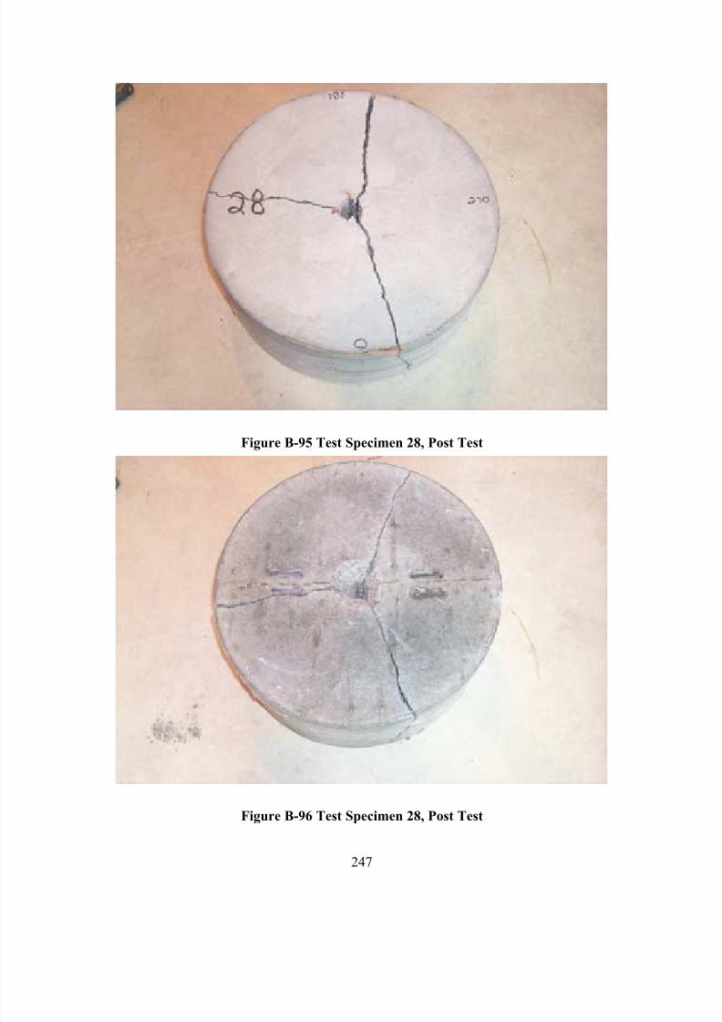
7/28/2019 Weathersby Dis
http://slidepdf.com/reader/full/weathersby-dis 264/280
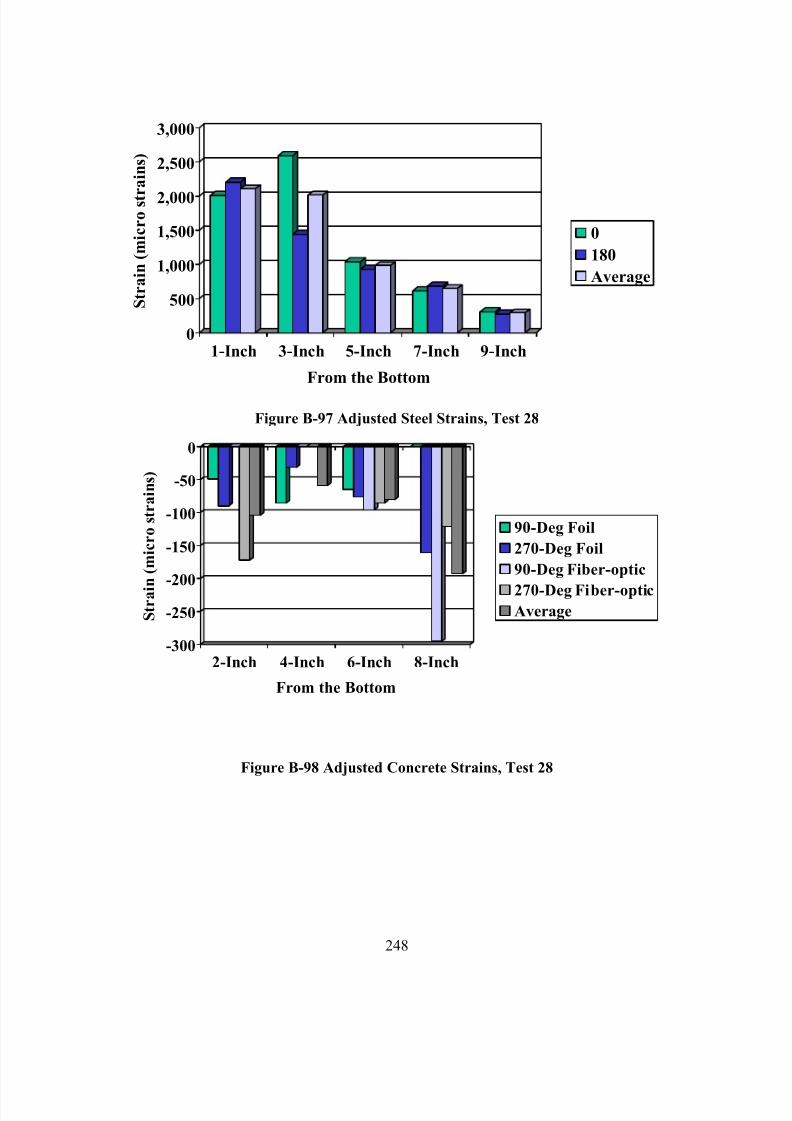
7/28/2019 Weathersby Dis
http://slidepdf.com/reader/full/weathersby-dis 265/280
248
0
500
1,000
1,500
2,000
2,500
3,000
S t r a i n ( m i c r o s t r a i n s )
1-Inch 3-Inch 5-Inch 7-Inch 9-Inch
From the Bottom
0
180
Average
Figure B-97 Adjusted Steel Strains, Test 28
-300
-250
-200
-150
-100
-50
0
S t r a i n ( m i c r o s t r a i n s )
2-Inch 4-Inch 6-Inch 8-Inch
From the Bottom
90-Deg Foil
270-Deg Foil
90-Deg Fiber-optic
270-Deg Fiber-opticAverage
Figure B-98 Adjusted Concrete Strains, Test 28
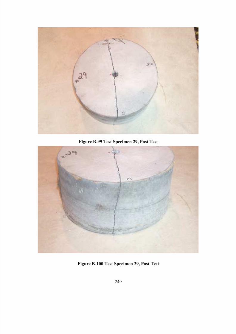
7/28/2019 Weathersby Dis
http://slidepdf.com/reader/full/weathersby-dis 266/280
249
Figure B-99 Test Specimen 29, Post Test
Figure B-100 Test Specimen 29, Post Test
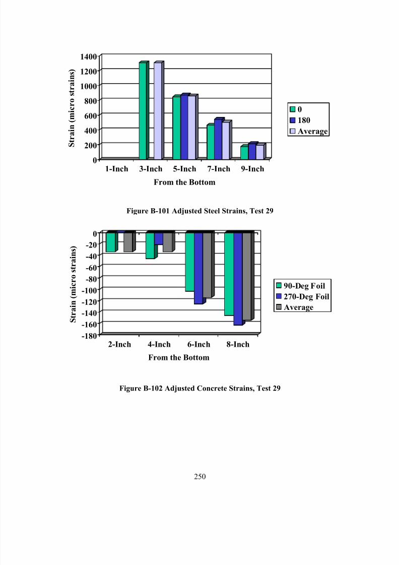
7/28/2019 Weathersby Dis
http://slidepdf.com/reader/full/weathersby-dis 267/280
250
0
200
400
600
800
1000
1200
1400
S t r a i n ( m i c r o
s t r a i n s )
1-Inch 3-Inch 5-Inch 7-Inch 9-Inch
From the Bottom
0
180
Average
Figure B-101 Adjusted Steel Strains, Test 29
-180
-160
-140
-120
-100
-80
-60
-40
-20
0
S t r a i n ( m i c r o s t r a i n s )
2-Inch 4-Inch 6-Inch 8-Inch
From the Bottom
90-Deg Foil
270-Deg FoilAverage
Figure B-102 Adjusted Concrete Strains, Test 29
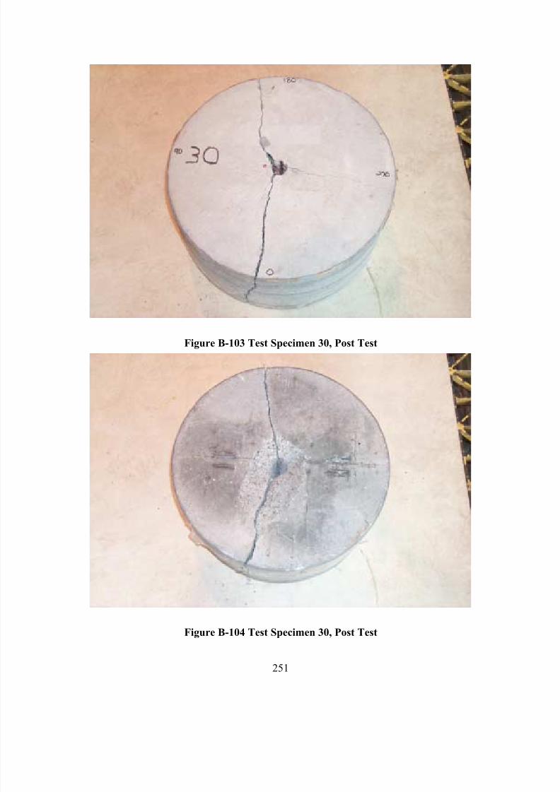
7/28/2019 Weathersby Dis
http://slidepdf.com/reader/full/weathersby-dis 268/280
251
Figure B-103 Test Specimen 30, Post Test
Figure B-104 Test Specimen 30, Post Test
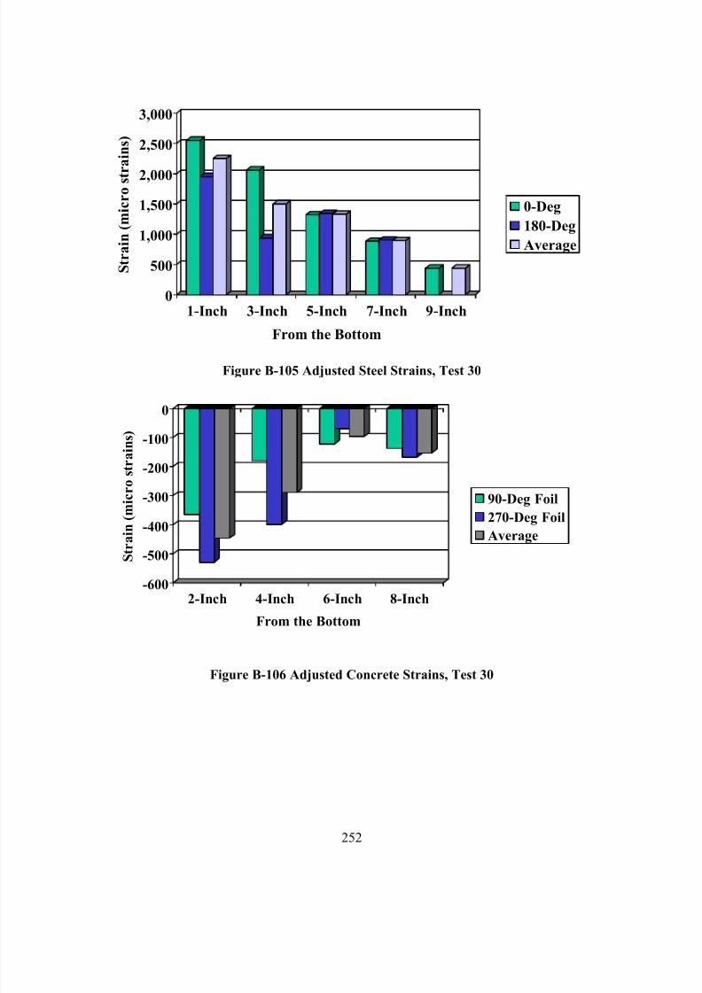
7/28/2019 Weathersby Dis
http://slidepdf.com/reader/full/weathersby-dis 269/280
252
0
500
1,000
1,500
2,000
2,500
3,000
S t r a i n ( m i c r o s t r a i n s )
1-Inch 3-Inch 5-Inch 7-Inch 9-Inch
From the Bottom
0-Deg
180-Deg
Average
Figure B-105 Adjusted Steel Strains, Test 30
-600
-500
-400
-300
-200
-100
0
S t r a i n ( m i c r o s t r a i n s )
2-Inch 4-Inch 6-Inch 8-Inch
From the Bottom
90-Deg Foil
270-Deg FoilAverage
Figure B-106 Adjusted Concrete Strains, Test 30
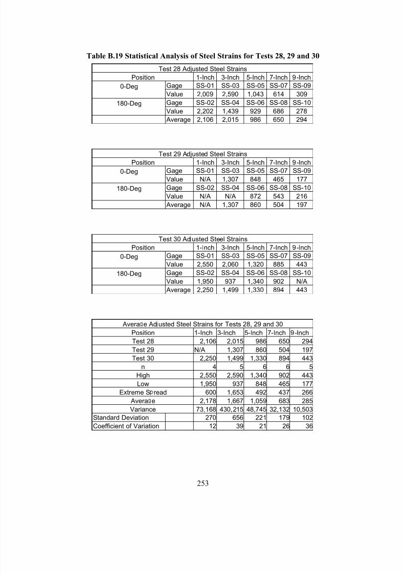
7/28/2019 Weathersby Dis
http://slidepdf.com/reader/full/weathersby-dis 270/280
253
Table B.19 Statistical Analysis of Steel Strains for Tests 28, 29 and 30
Test 28 Adjusted Steel Strains
Position 1-Inch 3-Inch 5-Inch 7-Inch 9-Inch
Gage SS-01 SS-03 SS-05 SS-07 SS-090-Deg
Value 2,009 2,590 1,043 614 309
Gage SS-02 SS-04 SS-06 SS-08 SS-10180-Deg
Value 2,202 1,439 929 686 278
Average 2,106 2,015 986 650 294
Test 29 Adjusted Steel Strains
Position 1-Inch 3-Inch 5-Inch 7-Inch 9-Inch
Gage SS-01 SS-03 SS-05 SS-07 SS-090-Deg
Value N/A 1,307 848 465 177
Gage SS-02 SS-04 SS-06 SS-08 SS-10180-Deg
Value N/A N/A 872 543 216
Average N/A 1,307 860 504 197
Test 30 Ad usted Steel Strains
Position 1-Inch 3-Inch 5-Inch 7-Inch 9-Inch
Gage SS-01 SS-03 SS-05 SS-07 SS-090-Deg
Value 2,550 2,060 1,320 885 443
Gage SS-02 SS-04 SS-06 SS-08 SS-10180-Deg
Value 1,950 937 1,340 902 N/A
Average 2,250 1,499 1,330 894 443
Avera e Ad usted Steel Strains for Tests 28, 29 and 30
Position 1-Inch 3-Inch 5-Inch 7-Inch 9-Inch
Test 28 2,106 2,015 986 650 294
Test 29 N/A 1,307 860 504 197
Test 30 2,250 1,499 1,330 894 443
n 4 5 6 6 5
High 2,550 2,590 1,340 902 443
Low 1,950 937 848 465 177
Extreme S read 600 1,653 492 437 266
Avera e 2,178 1,667 1,059 683 285Variance 73,168 430,215 48,745 32,132 10,503
Standard Deviation 270 656 221 179 102
Coefficient of Variation 12 39 21 26 36
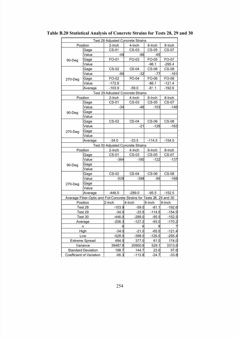
7/28/2019 Weathersby Dis
http://slidepdf.com/reader/full/weathersby-dis 271/280
254
Table B.20 Statistical Analysis of Concrete Strains for Tests 28, 29 and 30
Test 28 Adjusted Concrete Strains
Position 2-Inch 4-Inch 6-Inch 8-Inch
Gage CS-01 CS-03 CS-05 CS-07
Value -49 -86 -65
Gage FO-01 FO-03 FO-05 FO-0790-DegValue -96.1 -295.4
Gage CS-02 CS-04 CS-06 CS-08
Value -90 -32 -77 -161
Gage FO-02 FO-04 FO-06 FO-08270-DegValue -172.8 -86.1 -121.4
Average -103.9 -59.0 -81.1 -192.6
Test 29 Ad usted Concrete Strains
Position 2-Inch 4-Inch 6-Inch 8-Inch
Gage CS-01 CS-03 CS-05 CS-07
Value -34 -46 -103 -146
Gage90-DegValue
Gage CS-02 CS-04 CS-06 CS-08
Value -21 -126 -163
Gage270-DegValue
Average -34.0 -33.5 -114.5 -154.5
Test 30 Adjusted Concrete Strains
Position 2-Inch 4-Inch 6-Inch 8-Inch
Gage CS-01 CS-03 CS-05 CS-07
Value -364 -180 -122 -137
Gage90-DegValue
Gage CS-02 CS-04 CS-06 CS-08
Value -528 -398 -69 -168Gage270-DegValue
Average -446.0 -289.0 -95.5 -152.5
Average Fiber-Optic and Foil Concrete Strains for Tests 28, 29 and 30
Position 2-Inch 4-Inch 6-Inch 8-Inch
Test 28 -103.9 -59.0 -81.1 -192.6
Test 29 -34.0 -33.5 -114.5 -154.5
Test 30 -446.0 -289.0 -95.5 -152.5
Average -206.3 -127.2 -93.0 -170.2
n 6 6 8 7
High -34.0 -21.0 -65.0 -121.4
Low -528.0 -398.0 -126.0 -295.4Extreme Spread 494.0 377.0 61.0 174.0
Variance 39487.8 20950.6 529.1 3313.6
Standard Deviation 198.7 144.7 23.0 57.6
Coefficient of Variation -96.3 -113.8 -24.7 -33.8
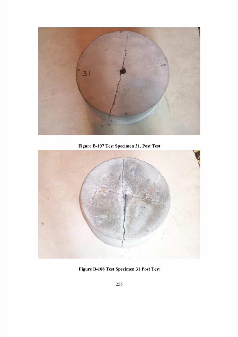
7/28/2019 Weathersby Dis
http://slidepdf.com/reader/full/weathersby-dis 272/280
255
Figure B-107 Test Specimen 31, Post Test
Figure B-108 Test Specimen 31 Post Test
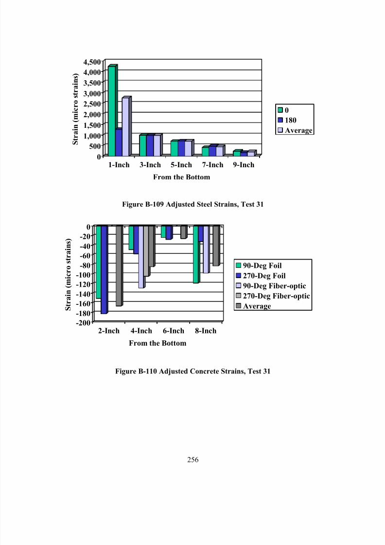
7/28/2019 Weathersby Dis
http://slidepdf.com/reader/full/weathersby-dis 273/280
256
0
500
1,000
1,500
2,000
2,5003,000
3,500
4,000
4,500
S t r a i n ( m i c r o s t r a i n s )
1-Inch 3-Inch 5-Inch 7-Inch 9-Inch
From the Bottom
0
180
Average
Figure B-109 Adjusted Steel Strains, Test 31
-200
-180
-160
-140-120
-100
-80
-60
-40
-20
0
S t r a i n ( m i c r o s t r a i n s )
2-Inch 4-Inch 6-Inch 8-Inch
From the Bottom
90-Deg Foil
270-Deg Foil
90-Deg Fiber-optic270-Deg Fiber-optic
Average
Figure B-110 Adjusted Concrete Strains, Test 31
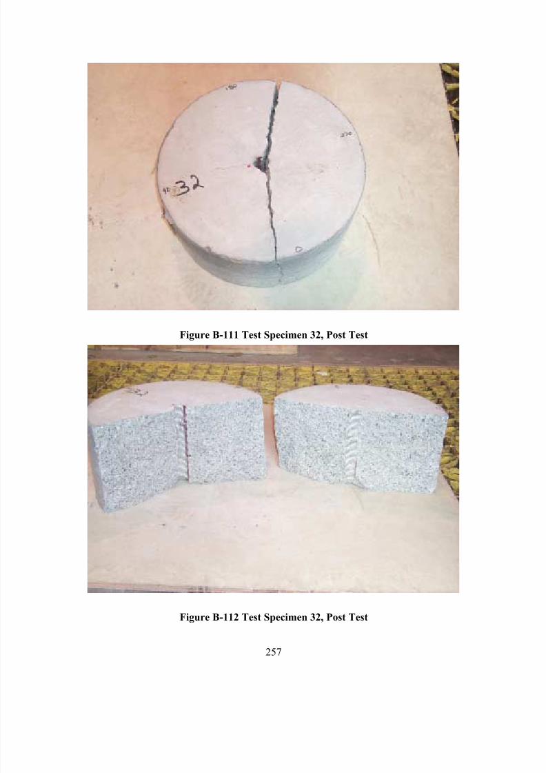
7/28/2019 Weathersby Dis
http://slidepdf.com/reader/full/weathersby-dis 274/280
257
Figure B-111 Test Specimen 32, Post Test
Figure B-112 Test Specimen 32, Post Test
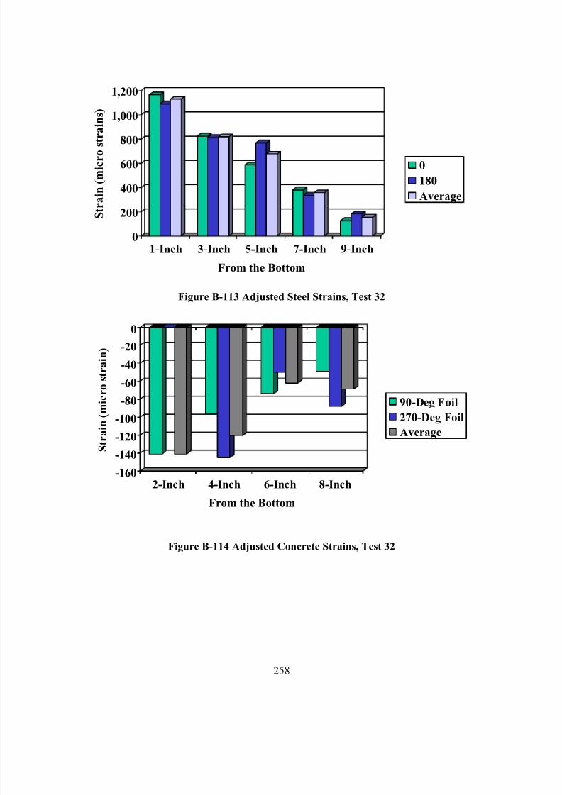
7/28/2019 Weathersby Dis
http://slidepdf.com/reader/full/weathersby-dis 275/280
258
0
200
400
600
800
1,000
1,200
S t r a i n ( m i c r o s t r a i n s )
1-Inch 3-Inch 5-Inch 7-Inch 9-Inch
From the Bottom
0
180
Average
Figure B-113 Adjusted Steel Strains, Test 32
-160
-140
-120
-100
-80
-60
-40
-20
0
S t r a i n ( m i c r o s t r a i n )
2-Inch 4-Inch 6-Inch 8-Inch
From the Bottom
90-Deg Foil
270-Deg FoilAverage
Figure B-114 Adjusted Concrete Strains, Test 32
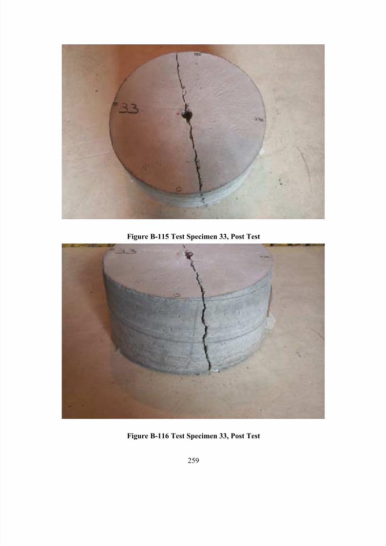
7/28/2019 Weathersby Dis
http://slidepdf.com/reader/full/weathersby-dis 276/280
259
Figure B-115 Test Specimen 33, Post Test
Figure B-116 Test Specimen 33, Post Test
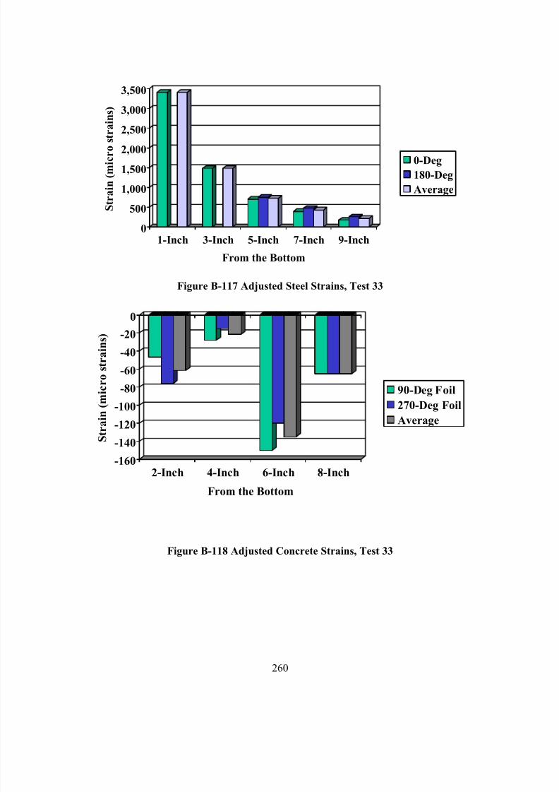
7/28/2019 Weathersby Dis
http://slidepdf.com/reader/full/weathersby-dis 277/280
260
0
500
1,000
1,500
2,000
2,500
3,000
3,500
S t r a i n ( m i c r o s t r a i n s )
1-Inch 3-Inch 5-Inch 7-Inch 9-Inch
From the Bottom
0-Deg
180-Deg
Average
Figure B-117 Adjusted Steel Strains, Test 33
-160
-140
-120
-100
-80
-60
-40
-20
0
S t r a i n
( m i c r o s t r a i n s )
2-Inch 4-Inch 6-Inch 8-Inch
From the Bottom
90-Deg Foil
270-Deg Foil
Average
Figure B-118 Adjusted Concrete Strains, Test 33
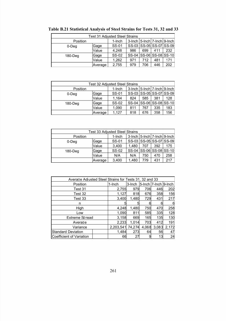
7/28/2019 Weathersby Dis
http://slidepdf.com/reader/full/weathersby-dis 278/280
261
Table B.21 Statistical Analysis of Steel Strains for Tests 31, 32 and 33
Test 31 Adjusted Steel Strains
Position 1-Inch 3-Inch 5-Inch 7-Inch 9-Inch
Gage SS-01 SS-03 SS-05 SS-07 SS-090-DegValue 4,248 986 699 411 232
Gage SS-02 SS-04 SS-06 SS-08 SS-10180-DegValue 1,262 971 712 481 171
Average 2,755 979 706 446 202
Test 32 Adjusted Steel Strains
Position 1-Inch 3-Inch 5-Inch 7-Inch 9-Inch
Gage SS-01 SS-03 SS-05 SS-07 SS-090-Deg
Value 1,164 824 585 381 128
Gage SS-02 SS-04 SS-06 SS-08 SS-10180-Deg
Value 1,090 811 767 335 183
Average 1,127 818 676 358 156
Test 33 Adjusted Steel Strains
Position 1-Inch 3-Inch 5-Inch 7-Inch 9-Inch
Gage SS-01 SS-03 SS-05 SS-07 SS-090-Deg
Value 3,400 1,480 707 392 175
Gage SS-02 SS-04 SS-06 SS-08 SS-10180-Deg
Value N/A N/A 750 470 258
Average 3,400 1,480 729 431 217
Avera e Ad usted Steel Strains for Tests 31, 32 and 33
Position 1-Inch 3-Inch 5-Inch 7-Inch 9-Inch
Test 31 2,755 979 706 446 202
Test 32 1,127 818 676 358 156
Test 33 3,400 1,480 729 431 217
n 5 5 6 6 6
High 4,248 1,480 750 470 258
Low 1,090 811 585 335 128
Extreme S read 3,158 669 165 135 130
Avera e 2,233 1,014 703 412 191
Variance 2,203,541 74,274 4,068 3,083 2,172
Standard Deviation 1,484 273 64 56 47
Coefficient of Variation 66 27 9 13 24
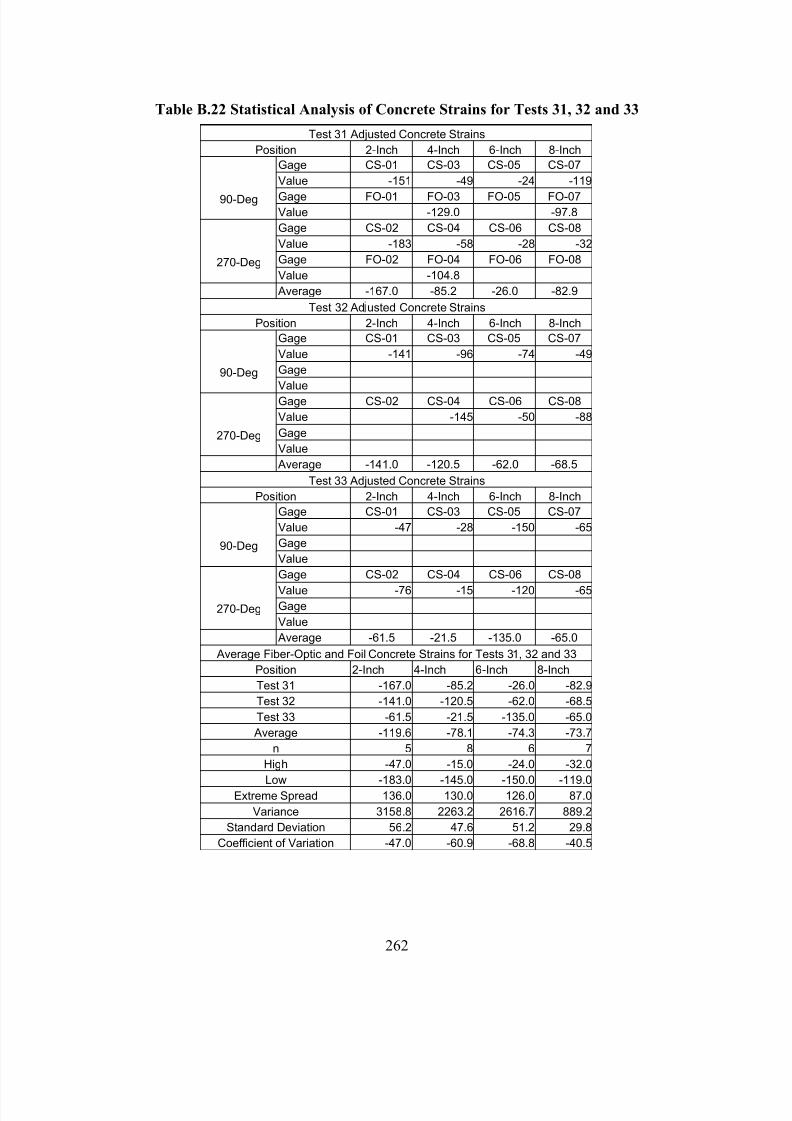
7/28/2019 Weathersby Dis
http://slidepdf.com/reader/full/weathersby-dis 279/280
262
Table B.22 Statistical Analysis of Concrete Strains for Tests 31, 32 and 33
Test 31 Adjusted Concrete Strains
Position 2-Inch 4-Inch 6-Inch 8-Inch
Gage CS-01 CS-03 CS-05 CS-07
Value -151 -49 -24 -119
Gage FO-01 FO-03 FO-05 FO-0790-DegValue -129.0 -97.8
Gage CS-02 CS-04 CS-06 CS-08
Value -183 -58 -28 -32
Gage FO-02 FO-04 FO-06 FO-08270-DegValue -104.8
Average -167.0 -85.2 -26.0 -82.9
Test 32 Ad usted Concrete Strains
Position 2-Inch 4-Inch 6-Inch 8-Inch
Gage CS-01 CS-03 CS-05 CS-07
Value -141 -96 -74 -49
Gage90-DegValue
Gage CS-02 CS-04 CS-06 CS-08
Value -145 -50 -88
Gage270-DegValue
Average -141.0 -120.5 -62.0 -68.5
Test 33 Adjusted Concrete Strains
Position 2-Inch 4-Inch 6-Inch 8-Inch
Gage CS-01 CS-03 CS-05 CS-07
Value -47 -28 -150 -65
Gage90-DegValue
Gage CS-02 CS-04 CS-06 CS-08
Value -76 -15 -120 -65Gage270-DegValue
Average -61.5 -21.5 -135.0 -65.0
Average Fiber-Optic and Foil Concrete Strains for Tests 31, 32 and 33
Position 2-Inch 4-Inch 6-Inch 8-Inch
Test 31 -167.0 -85.2 -26.0 -82.9
Test 32 -141.0 -120.5 -62.0 -68.5
Test 33 -61.5 -21.5 -135.0 -65.0
Average -119.6 -78.1 -74.3 -73.7
n 5 8 6 7
High -47.0 -15.0 -24.0 -32.0
Low -1
83.0 -145.0 -
150.0 -
119.0Extreme Spread 136.0 130.0 126.0 87.0
Variance 3158.8 2263.2 2616.7 889.2
Standard Deviation 56.2 47.6 51.2 29.8
Coefficient of Variation -47.0 -60.9 -68.8 -40.5
7/28/2019 Weathersby Dis
http://slidepdf.com/reader/full/weathersby-dis 280/280
VITA