VOLUMETRIC SURVEYOF

LAKE HALBERT

Prepared for:

CITY OF CORSICANA

Prepared by:

The Texas Water Development Board

March 10, 2003

Texas Water Development Board

Craig D. Pedersen, Executive Administrator

Texas Water Development Board

William B. Madden, Chairman Noe Fernandez, Vice-ChairmanElaine M. Barrón, M.D Jack HuntCharles L. Geren Wales H. Madden Jr.

Authorization for use or reproduction of any original material contained in this publication, i.e.not obtained from other sources, is freely granted. The Board would appreciate acknowledgment.

This report was prepared by the Hydrographic Survey group:

Ruben S. Solis, Ph.D., P.E.Duane ThomasRandall BurnsMarc Sansom

Published and Distributedby the

Texas Water Development BoardP.O. Box 13231

Austin, Texas 78711-3231

TABLE OF CONTENTS

INTRODUCTION ............................................................................................................................1

LAKE HISTORY AND GENERAL INFORMATION.....................................................................1

HYDROGRAPHIC SURVEYING TECHNOLOGY ........................................................................3

PRE-SURVEY PROCEDURES .......................................................................................................3

SURVEY PROCEDURES................................................................................................................4

Equipment Calibration and Operation..................................................................................4Field Survey.........................................................................................................................5Data Processing....................................................................................................................6

RESULTS.........................................................................................................................................8

SUMMARY......................................................................................................................................8

REFERENCES.................................................................................................................................9

APPENDICES

APPENDIX A - LAKE HALBERT VOLUME TABLEAPPENDIX B - LAKE HALBERT AREA TABLEAPPENDIX C - LAKE HALBERT ELEVATION-AREA- VOLUME GRAPHAPPENDIX D - CROSS-SECTION PLOTSAPPENDIX E - DEPTH SOUNDER ACCURACYAPPENDIX F - GPS BACKGROUND

LIST OF FIGURES

FIGURE 1 - LOCATION MAPFIGURE 2 - LOCATION OF SURVEY DATAFIGURE 3 - SHADED RELIEFFIGURE 4 - DEPTH CONTOURSFIGURE 5 - CONTOUR MAP

1

LAKE HALBERTHYDROGRAPHIC SURVEY REPORT

INTRODUCTION

Staff of the Hydrographic Survey Unit of the Texas Water Development Board (TWDB)

conducted a hydrographic survey of Lake Halbert during the period of February 10, 11 and 22, 1999.

The purpose of the survey was to determine the volume of the lake at the conservation pool elevation.

From this information, future surveys will be able to determine the location and rates of sediment

deposition in the conservation pool over time. Survey results are presented in the following pages

in both graphical and tabular form. All elevations presented in this report will be reported in feet

above mean sea level based on the National Geodetic Vertical Datum of 1929 (NGVD '29) unless the

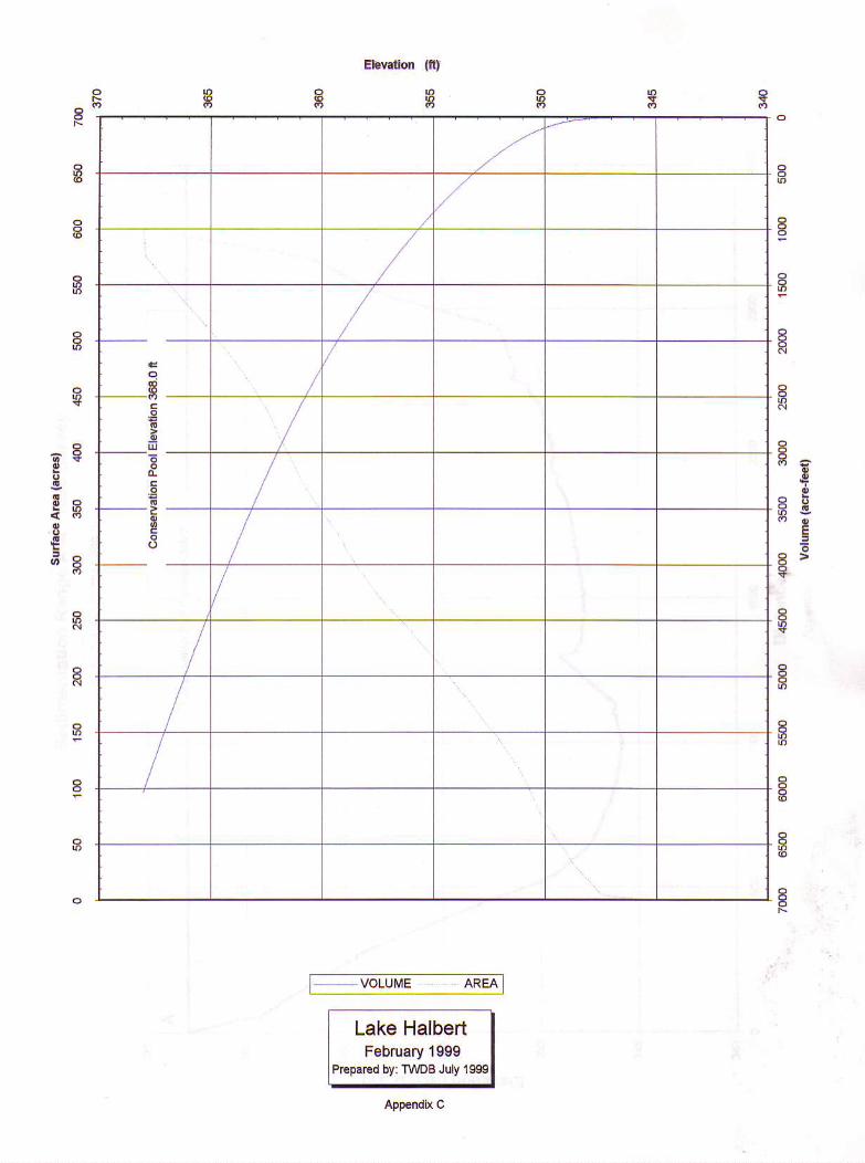
elevation is noted otherwise. The conservation pool elevation for Lake Halbert is 368.0 feet. Past

design information from TWDB (1974) estimated the surface area at this elevation to be 650 acres and

the storage volume to be 7,420 acre-feet of water.

LAKE HISTORY AND GENERAL INFORMATION

Historical information on Lake Halbert was obtained from Texas Water Development

Board reports (TWDB 1967; TWDB 1974). The City of Corsicana owns the water rights to Lake

Halbert and operates and maintains associated Halbert Dam. The lake is located on Little Elm Creek

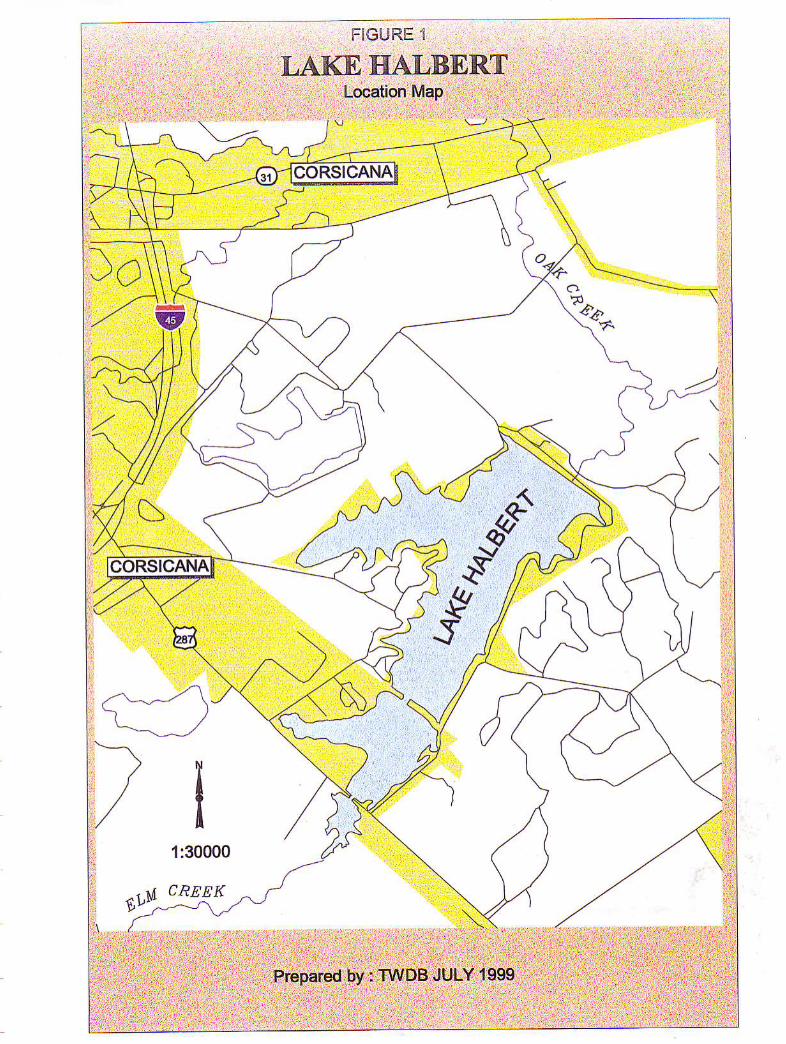
(Trinity River basin) in Navarro County, four miles southeast of Corsicana, Texas (see Figure 1).

Records indicate the drainage area is approximately 12 square miles with supplemental pumping from

Chambers Creek. At the conservation pool elevation, the lake has approximately 11.2 miles of

shoreline and is 2.23 miles long. The widest point of the reservoir is approximately 0.74 miles

(located 0.5 miles upstream of the dam).

2

Water Rights Permit No. 803 (Application No. 841) was issued to City of Corsicana on July

1, 1925 and authorized the construction of a dam to impound and use 7,653 acre-feet of water for

municipal purposes. On April 14, 1950 Permit No. 1534 (Application No. 1644) allowed the owner

to raise the spillway one foot and allowed diversion of 3,650 acre-feet of water annually from

Chambers Creek. The Texas Water Commission issued Certificate of Adjudication No. 08-5030 on

May 5, 1987. The certificate authorizes the City of Corsicana to maintain an existing dam and

reservoir on Little Elm Creek (Lake Halbert) and to impound not to exceed 7,357 acre-feet of water.

The owner was authorized to divert and use not to exceed 4,003 acre-feet of water per year from Lake

Halbert for municipal purposes. Under the Special Conditions section of the Certificate, the owner

is authorized to store water diverted from Richland Creek Reservoir (Richland Chambers Reservoir)

in Lake Halbert for subsequent diversion and use to the extent authorized.

Records indicate the construction for Lake Halbert and Halbert Dam started in 1920 and was

completed in 1921. Deliberate impoundment began that same year. The design engineer for the

facility was J. W. Harrison.

Halbert Dam and appurtenant structures consist of a rolled-earthfill embankment 2,780 feet

in length, with a maximum height of 49 feet and a crest elevation of 375.0 feet. The service spillway

is an uncontrolled concrete chute located to the left (west) of the embankment. The crest of the

spillway is 175 feet in length at elevation 368.0 feet. Records indicate a 24-inch diameter conduit that

passes through the dam is valve controlled for releases to the water treatment plant and for

downstream releases.

The estimated volume of Lake Halbert in 1921 at conservation pool elevation 367.0 feet was

8,010 acre-feet, and the surface area 593 acres. In 1949 the U. S. Soil Conservation Service

performed a sediment survey. Results indicated the siltation had reduced the lake volume by 1,355

acre-feet of water, corresponding to an average loss of 48.4 acre-feet per year between 1921 and

1949. In 1950 the service spillway was raised one foot to elevation 368.0 feet. The surface area of

the lake was then estimated to be 650 acres and the volume to be 7,420 acre-feet.

3

HYDROGRAPHIC SURVEYING TECHNOLOGY

The equipment used in the performance of the hydrographic survey consists of a 23-foot

aluminum tri-hull SeaArk craft with cabin, equipped with twin 90-Horsepower Johnson outboard

motors. Installed within the enclosed cabin are an Innerspace Helmsman Display (for navigation), an

Innerspace Technology Model 449 Depth Sounder and Model 443 Velocity Profiler, a Trimble

Navigation, Inc. 4000SE GPS receiver, an OmniSTAR receiver, and an on-board 486 computer. A

water-cooled generator provides electrical power through an in-line undisturbed power supply.

Reference to brand names does not imply endorsement by the TWDB.

The GPS equipment, survey vessel, and depth sounder combine together to provide an efficient

hydrographic survey system. As the boat travels across the lake surface, the depth sounder takes

approximately ten readings of the lake bottom each second. The depth readings are stored on the

survey vessel's on-board computer along with the corrected positional data generated by the boat's

GPS receiver. The daily data files collected are downloaded from the computer and brought to the

office for editing after the survey is completed. During editing, bad data is removed or corrected,

multiple data points are averaged to get one data point per second, and average depths are converted

to elevation readings based on the lake elevation recorded on the day the survey was performed.

Accurate estimates of the lake volume can be quickly determined by building a 3-D model of the

reservoir from the collected data. The level of accuracy is equivalent to or better than previous

methods used to determine lake volumes, some of which are discussed in Appendix F.

PRE-SURVEY PROCEDURES

The reservoir's surface area was determined prior to the survey by digitizing with AutoCad

software the lake's pool boundary (elevation 368.0 feet). The boundary file was created from the 7.5-

minute USGS quadrangle map, Corsicana, TX. (1965), Photo-revised 1978. The survey layout was

designed by placing survey track lines at 500-foot intervals across the lake. The survey design for this

lake required approximately 37 survey lines to be placed along the length of the lake.

4

SURVEY PROCEDURES

The following procedures were followed during the hydrographic survey of Lake Halbert

performed by the TWDB. Information regarding equipment calibration and operation, the field survey,

and data processing is presented.

Equipment Calibration and Operation

At the beginning of each surveying day, the depth sounder was calibrated with the Innerspace

Velocity Profiler, an instrument that measures the local speed of sound. The average speed of sound

in the water column extending below the boat-mounted transducers (at the boat's draft of 1.2 ft) to the

lake bottom was determined by averaging local speed-of-sound measurements collected by the

velocity profiler through the water column. The velocity profiler probe was first placed in the water

to moisten and acclimate the probe. The probe was next raised to the water surface where the depth

was zeroed. The probe was then gradually lowered on a cable to a depth just above the lake bottom,

and then raised to the surface. During this time the unit measured the local speed of sound. The

average of the measurements was next computed and displayed by the unit. The displayed value of

the average speed of sound was entered into the ITI449 depth sounder, which then provided the depth

of the lake bottom. The depth was then checked manually with a measuring tape to ensure that the

depth sounder was properly calibrated and operating correctly. Based on the measured speed of sound

for various depths and the average speed of sound calculated for the entire water column, the depth

sounder is accurate to within +0.2 feet. An additional estimated error of +0.3 feet arises due to the

variation in boat inclination. These two factors combine to give an overall accuracy of +0.5 feet for

any instantaneous reading. These errors tend to be minimized over the entire survey, since some

readings are positive and some are negative. Further information on these calculations is presented

in Appendix F.

During the survey, the onboard GPS receiver was set to a horizontal mask of 10° and a PDOP

(Position Dilution of Precision) limit of 7 to maximize the accuracy of horizontal positions. An

internal alarm sounds if the PDOP rises above seven to advise the field crew that the horizontal

5

position has degraded to an unacceptable level. The lake’s initialization file used by the Hypack data

collection program was set up to convert the collected DGPS positions on the fly to state plane

coordinates. Both sets of coordinates were then stored in the survey data file.

Field Survey

Data were collected at Lake Halbert on February 10, 11 and 22, 1999. During data collection,

the crew had excellent weather with moderate temperatures and mild winds. Approximately 8,475

data points were collected over the 12.7 miles traveled. These points were stored digitally on the

boat's computer in over 22 data files. Data were not collected in areas with significant obstructions

unless these areas represented a large amount of water. Figure 2 shows the actual location of all data

collection points. The first two days of data collection were in the upper reaches of Lake Halbert

where a smaller boat was used to gain access upstream of the railroad trestle and State Highway 287

bridge on Elm Creek. The small boat was also used to collect data upstream of a retention dam

located on the north arm of the lake. The larger survey vessel was used in the main body of the lake.

Elm Creek flows in a southwest to northeast direction with Halbert Dam being at the northeast

end of the lake basin. TWDB staff observed the land surrounding the lake to be generally flat to

rolling hills. There was no residential or commercial development around the perimeter of the lake.

The City of Corsicana owns the surrounding land around Lake Halbert. A city park along with a

fishing pier and boat ramp facilities is located along the northwest shoreline of the lake.

While performing the survey on the lake, the field crew noted on the depth sounder chart that

the bathymetry or contour of the lake bottom reflected the characteristics of the terrain surrounding the

lake. A gradual slope was noticed as the boat traveled from the shoreline to the center of the lake.

There was no defined channel or thalweg of Elm Creek in the main body of the lake. Between Halbert

Dam and the railroad trestle, the crew noted extensive shoreline erosion on the east bank.

As the field crew collected data in the upper reaches of Elm Creek, navigational hazards such

as submerged trees and stumps became apparent. In addition, sediment deposits and standing

vegetation were observed. The crew was able to collect data in these areas, but at a much slower

6

pace. Data collection in the headwaters was limited when the boat could no longer cross the lake due

to shallow water and extensive vegetation.

The collected data were stored in individual data files for each pre-plotted range line or

random data collection event. These files were downloaded to diskettes at the end of each day for

future processing.

Data Processing

The collected data were downloaded from diskettes onto the TWDB's computer network. Tape

backups were made for future reference as needed. To process the data, the EDIT routine in the

Hypack Program was run on each raw data file. Data points such as depth spikes or data with missing

depth or positional information were deleted from the file. A correction for the lake elevation at the

time of data collection was also applied to each file during the EDIT routine. During the survey, the

water surface remained at conservation pool elevation of 368.0 feet. After all changes had been made

to the raw data file, the edited file was saved with a different extension. The edited files were

combined into a single X,Y,Z data file, to be used with the GIS software to develop a model of the

lake's bottom surface.

The resulting data file was downloaded to a Sun Sparc 20 workstation running the UNIX

operating system. Environmental System Research Institute’s (ESRI) Arc/Info GIS software was used

to convert the data to a MASS points file. The MASS points and the boundary file were then used

to create a Digital Terrain Model (DTM) of the reservoir's bottom surface using Arc/Info's TIN

software module. The module generates a triangulated irregular network (TIN) network from the data

points and the boundary file using a method known as Delauney's criteria for triangulation. A triangle

is formed between three non-uniformly spaced points, including all points along the boundary. If there

is another point within the triangle, additional triangles are created until all points lie on the vertex

of a triangle. All of the data points are used in this method. The generated network of three-

dimensional triangular planes represents the actual bottom surface. With this representation of the

bottom, the software then calculates elevations along the triangle surface plane by determining the

elevation along each leg of the triangle. The reservoir area and volume can be determined from the

7

triangulated irregular network created using this method of interpolation.

If data points were collected outside the digitized boundary, the boundary was modified to

include the data points. The boundary file in areas of significant sedimentation was also downsized

as deemed necessary based on the data points and the observations of the field crew. The resulting

boundary shape was used to develop each of the map presentations of the lake in this report.

There were some areas where volume and area values could not be calculated by interpolation

because of a lack of information within the reservoir. "Flat triangles" were drawn at these locations.

Arc/Info does not use flat triangle areas in the volume or contouring features of the model. These

areas were determined to be insignificant for this project, therefore no additional points were needed

to allow for interpolation and contouring of the entire lake surface at elevation 368.0. Volumes and

areas were calculated from the TIN for the entire reservoir at one-tenth of a foot intervals. From

elevation 343.2 to elevation 368.0, the surface areas and volumes of the lake were computed using

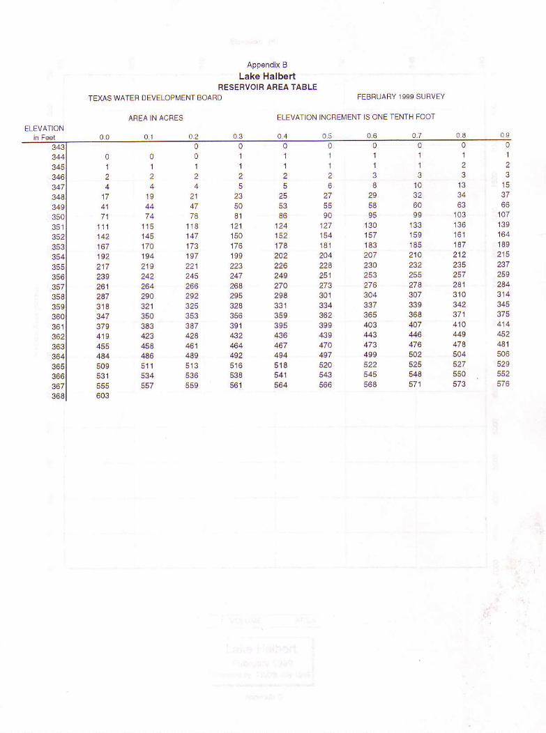
Arc/Info software. The computed area of the lake at elevation 368.0 was 603 surface acres. The

computed area was 47 surface acres less than originally calculated in 1950 (Texas Water

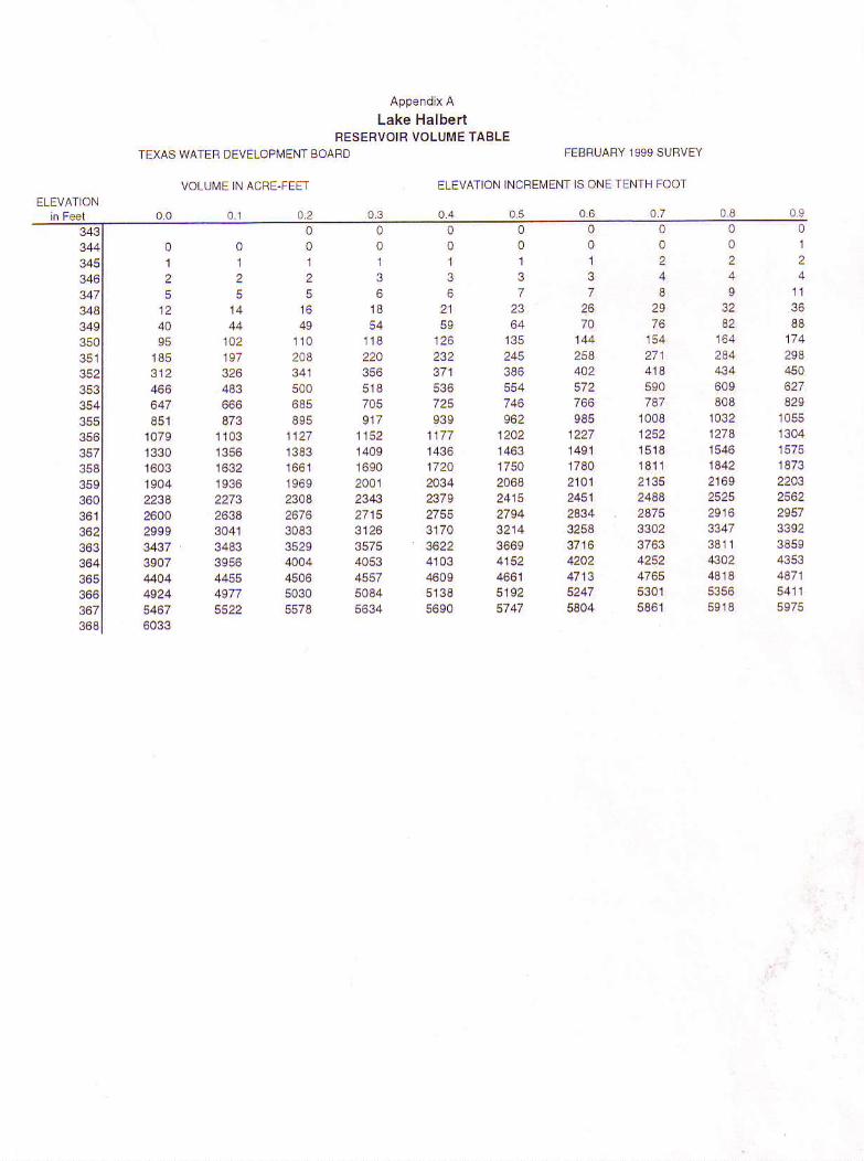
Development Board, 1967). The computed reservoir volume table is presented in Appendix A and

the area table in Appendix B. An elevation-area-volume graph is presented in Appendix C.

Other products developed from the model include a shaded relief map and a shaded depth

range map. To develop these maps, the TIN was converted to a lattice using the TINLATTICE

command and then to a polygon coverage using the LATTICEPOLY command. Using the

POLYSHADE command, colors were assigned to the range of elevations represented by the polygons

that varied from navy to yellow. The lower elevation was assigned the color of navy, and the 368.0

lake elevation was assigned the color of yellow. Different color shades were assigned to the

intermediate depths. Figure 3 presents the resulting depth shaded representation of the lake. Figure

4 presents a similar version of the same map, using bands of color for selected depth intervals.

Linear filtration algorithms were then applied to the DTM smooth cartographic contours. The

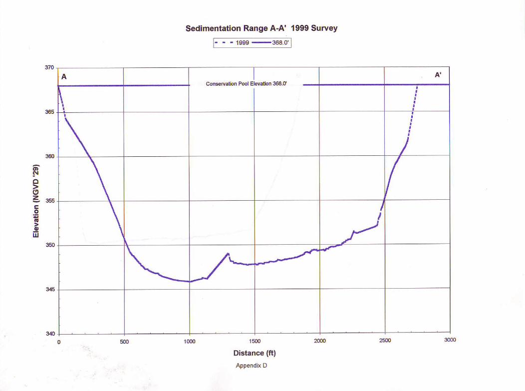
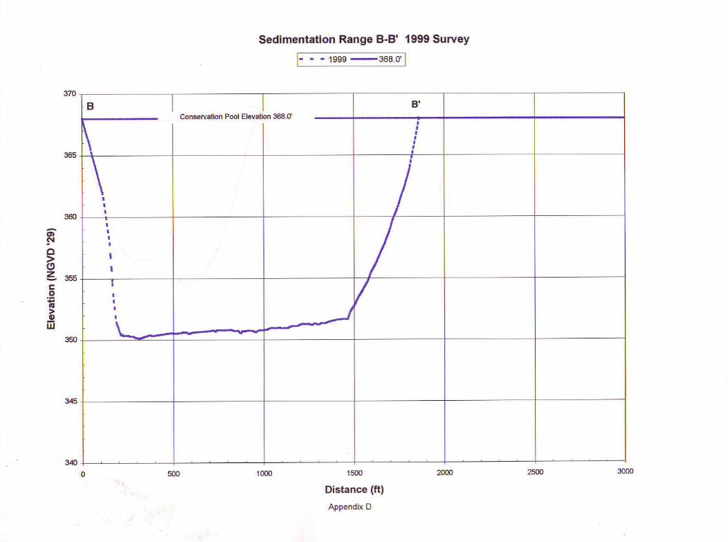
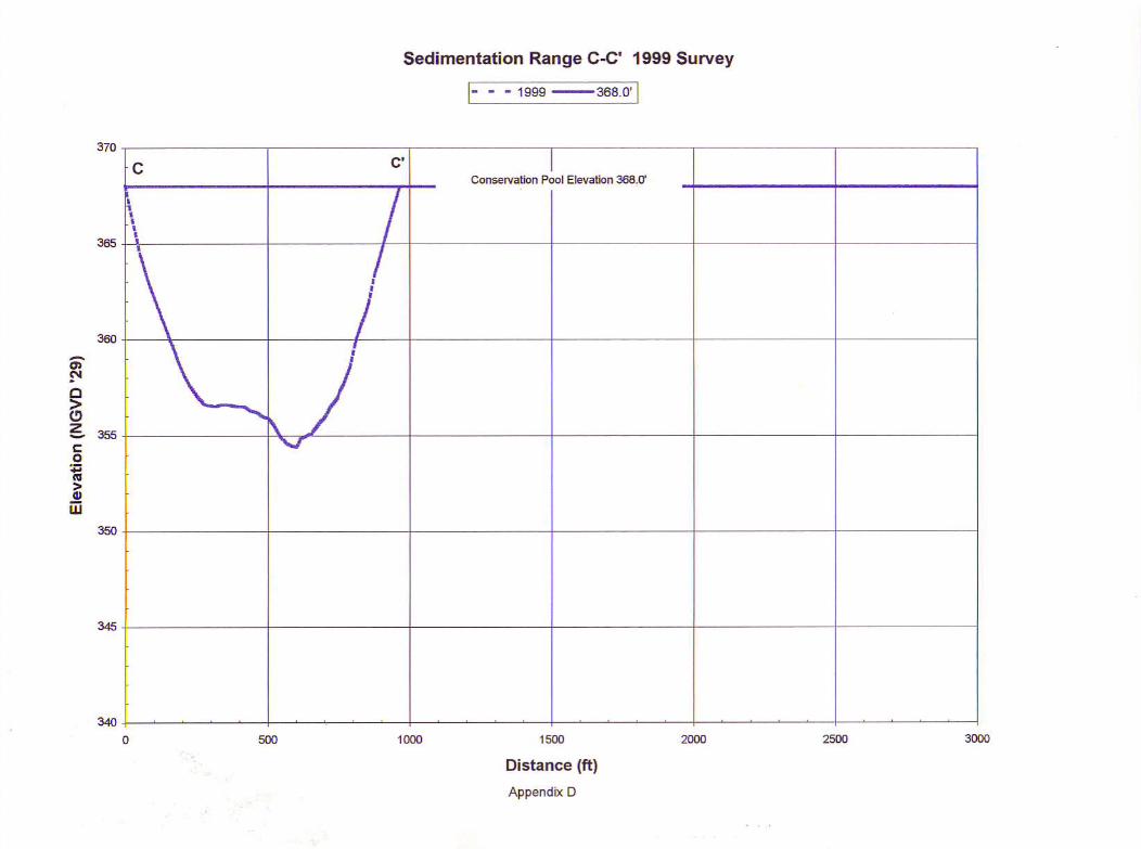
resulting contour map of the bottom surface at two-foot intervals is presented in Figure 5.

8

RESULTS

Results from the 1999 TWDB survey indicate Lake Halbert encompasses 603 surface acres

and contains a total volume of 6,033 acre-feet at the conservation pool elevation of 368.0 feet. The

shoreline at this elevation was calculated to be 11.2 miles. The deepest point of the lake, elevation

343.2 feet and corresponding to a depth of 24.8 feet, was located approximately 170 feet upstream

from the center of Lake Halbert Dam.

SUMMARY

Lake Halbert was initially impounded in 1921. Storage calculations in 1950 estimated the

volume at conservation pool elevation 368.0 feet to be 7,420 acre-feet with a surface area of 650

acres.

During the period February 10, 11 and 22, 1999, a hydrographic survey of Lake Halbert was

performed by the Texas Water Development Board's Hydrographic Survey Program. The 1999 survey

used technological advances such as differential global positioning and geographical information

system technology to model the reservoir's bathymetry. These advances allowed a survey to be

performed quickly and to collect significantly more bathymetric data on Lake Halbert than previous

survey methods. Results indicate that the lake's volume at the conservation pool elevation of 368.0

feet is 6,033 acre-feet with an area of 603 acres.

The estimated reduction in storage volume at the conservation pool elevation of 368.0 feet

since 1950 is 1,387 acre-feet, or roughly 28.3 acre-feet per year, significantly less than the estimated

loss rate between 1921 and 1949 of 48.4 acre-feet per year (TWDB, 1967). The average annual

deposition rate of sediment in the conservation pool of the reservoir can be estimated at 2.36 acre-feet

per square mile of drainage area. (Please note that this is just a mathematical estimate based on

differences between past and current surveys.)

9

It is difficult to compare the original design area and volume for Lake Halbert to that

determined by the current TWDB survey because little is known about the original design method, the

amount of data collected, and the method used to process the collected data. However, TWDB

considers the 1999 survey to be a significant improvement over previous survey procedures and

recommends that the same methodology be used in five to ten years or after major flood events to

monitor changes to the lake's storage volume.

REFERENCES

Texas Water Development Board. 1967. Dams and reservoirs in Texas, historical and descriptive

information, Report 48, June 1967.

Texas Water Development Board. 1974. Engineering data on dams and reservoirs in Texas. Part II.

Report 126. October 1974.

IIIIttIIIIIttIItIII

TEXAS WAIER DEVELOPMENI BOA RD

VOLUME IN ACFE.FEET

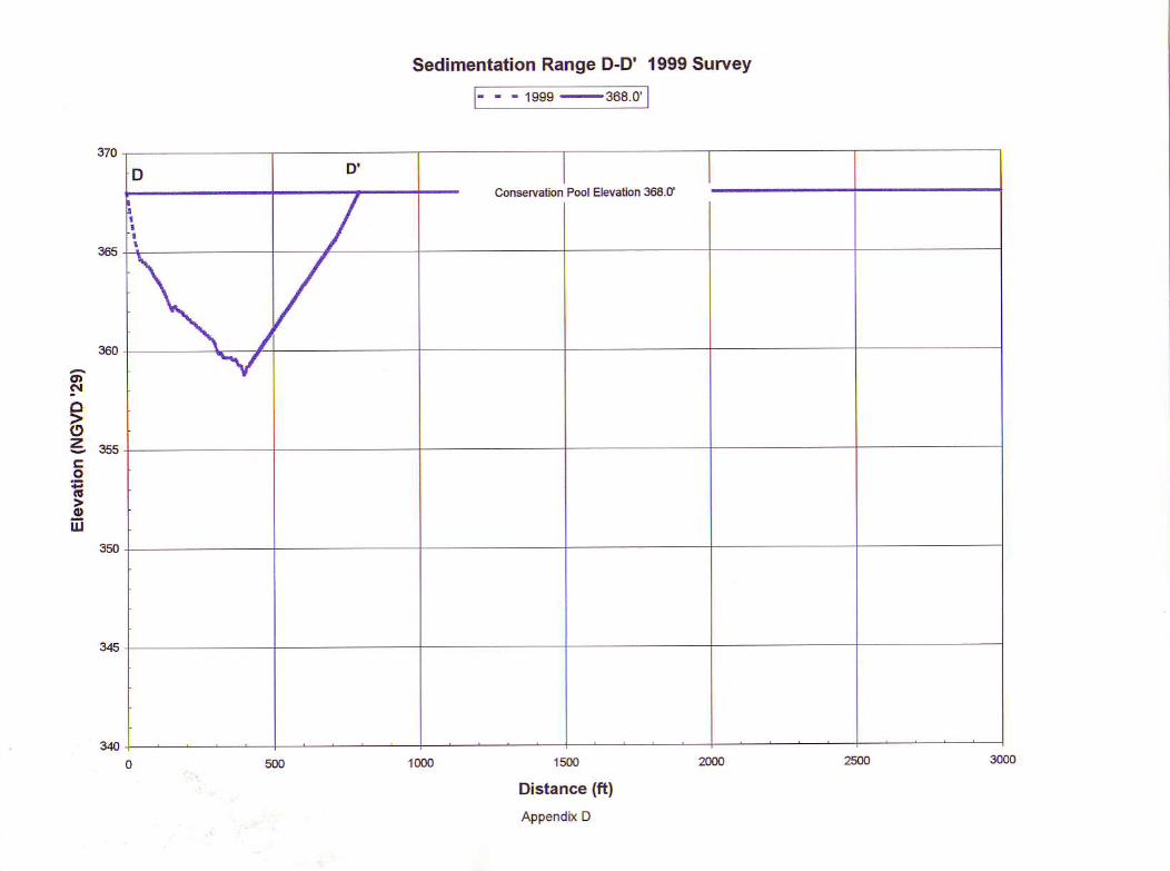
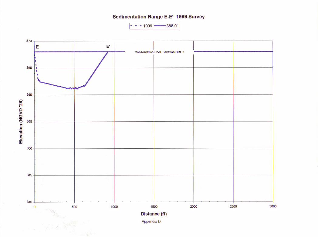
Appendix ALake Halbert

RESEBVOIB VOLUII/IE TABLEFEBFUARY 1999 SUBVEY

ELEVATION INCREMENI IS ONETENTH FOOTELEVATON

353

345346347348349350

352

012

36

002

932

002

8

00137

2670

258402572766985

1227

0013

2364

1 3 5

00

36

2 1

00136

o 200125

1 649

1 1 0208341

0125

102

0125

'12

356

361362353

951 8 5312466647851

107913301603190422382600299934373907

492454676033

'197

483666

1 1 0 313561632193622732638304134833956445549n

500685895

'1127

1383166119692308

30633529400445065030

1 854

1 1 82203565 1 8705917

1 1 5 2144916902001234327153126

4053455750845634

59126232371536725939

1 1 7 71436172020342379

3170

4103460951385690

245386554746

12421463175020682415279432143669415246615 1 9 25747

14911780210124512934325837164242471352475804

29

1 5 4271

590

100812521 5 1 81 8 1 121352484

3302

4252476553015861

8?164244434609808

10321278154518422169

2916

38i I43024 8 1 8

5 9 1 8

88

298€0427829

1055130415751873

2957339238594353487154115975367

368

Lake HalbertRESEBVOIF ABEA TABLE

IIIIIIIIIIIIIIIIIII

TEXAS WATER DEVELOPMEN'I SOAFO

AREA IN ACRES

FEBFUARY 19SS SURVEY

ELEVATION INCBEI,IENT IS ONETENTH FOOIELEVATION

0123

1 53766a73964

0123

1 33463

1 0 3

01

25

23

012

1 7

1 8 9215237259284314345

452481506529552576

711 1 1142

1922 1 7239261247

508 1

121150

1 9 9

861241 5 217e242226249270298

3954364674945 1 8541564

6099

1 5 91 8 5214232255278307339368447446476502525548571

1872 1 2235

2413 1 0342371

0I13

1 032

0113I

295895

1 3 0

6275590

1271541 8 1204224251273301334362399€ 9474497520543

01125

2553

0 20012

21

781 1 8

266292

3533874284614895 1 3

559

012

1 9

1 1 51451741 9 4219242264294321350383

4865 1 1534

349350351352353

344345346347348

363364

366367968

4 1 0449478504527550

223247264295328356391+32

4925 1 6538561

173

245

1 8 3207230253

34433736540344347349952254556E

356

358

360361362

3 1 83473794 1 9

484

531555603

E.9

E

E

3

ttIItII

tIIIIIItI

a

Erevation ft'

e

I g q- 3

C a

I < r ,r €

l i 'I

ib

R

R

I^ EH E

E!

i6

R

R

6

3

Lake HalbertFebmary 1999

P€pared by: TII/DB July 1999

tr- voLUMa---- AREA'-I

FPg

r-

n|

6

Ee

oIoo(Do+oC'

GEoGIEEoo

IIIIIIIItttIIIJ6

IIIITI

eI

aR

I

{ez. otgN) uo$a e|f

k

F{\

qdEtl

Fng

E-

g r

8€

FI

(,ttnooobooodc,o'€GIttooE

;g

R$

(62

, g g

M u

o$

E a

t3

b

l

o

itK6l

IIIIIIIa

If

;:

;o

rE

r€

I€

TU

'

TTIIII

Eg

!=

gE

6<

lt

E

(62. O/'\gN

) uonEm

|3

ittEfid9Ed

t,

,

o

RP

IIIIIttIIIItItItltl

ap

:'

:=

-

o*

o<

Q'

tU)

ototooc.G0,(,(t,

?5ii5

n3

FH

(62

, oAg

N) uo

lle^a

t3

IE#EEI3l5II

----?'

l

8q

r:

F.

E.

9E

o<

IooooutulE')

t!a,{to

R6

ntde!6IUJ

u.l

IttIIIIIttIITItIItI

II

EH

(62

, OA

9N

) uo

lle^a

tf

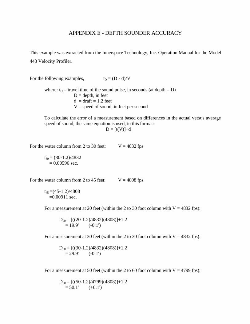
APPENDIX E - DEPTH SOUNDER ACCURACY

This example was extracted from the Innerspace Technology, Inc. Operation Manual for the Model

443 Velocity Profiler.

For the following examples, tD = (D - d)/V

where: tD = travel time of the sound pulse, in seconds (at depth = D)D = depth, in feetd = draft = 1.2 feetV = speed of sound, in feet per second

To calculate the error of a measurement based on differences in the actual versus averagespeed of sound, the same equation is used, in this format:

D = [t(V)]+d

For the water column from 2 to 30 feet: V = 4832 fps

t30 = (30-1.2)/4832 = 0.00596 sec.

For the water column from 2 to 45 feet: V = 4808 fps

t45 =(45-1.2)/4808 =0.00911 sec.

For a measurement at 20 feet (within the 2 to 30 foot column with V = 4832 fps):

D20 = [((20-1.2)/4832)(4808)]+1.2 = 19.9' (-0.1')

For a measurement at 30 feet (within the 2 to 30 foot column with V = 4832 fps):

D30 = [((30-1.2)/4832)(4808)]+1.2 = 29.9' (-0.1')

For a measurement at 50 feet (within the 2 to 60 foot column with V = 4799 fps):

D50 = [((50-1.2)/4799)(4808)]+1.2 = 50.1' (+0.1')

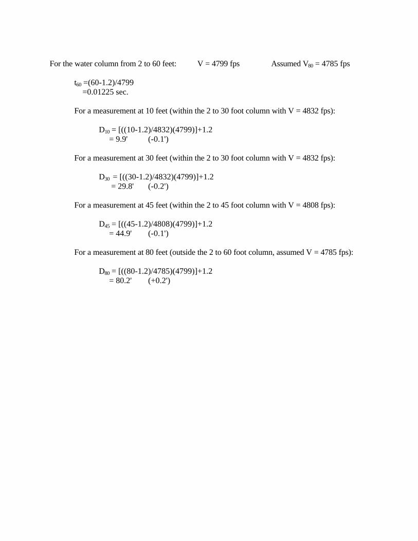
For the water column from 2 to 60 feet: V = 4799 fps Assumed V80 = 4785 fps

t60 =(60-1.2)/4799 =0.01225 sec.

For a measurement at 10 feet (within the 2 to 30 foot column with V = 4832 fps):

D10 = [((10-1.2)/4832)(4799)]+1.2 = 9.9' (-0.1')

For a measurement at 30 feet (within the 2 to 30 foot column with V = 4832 fps):

D30 = [((30-1.2)/4832)(4799)]+1.2 = 29.8' (-0.2')

For a measurement at 45 feet (within the 2 to 45 foot column with V = 4808 fps):

D45 = [((45-1.2)/4808)(4799)]+1.2 = 44.9' (-0.1')

For a measurement at 80 feet (outside the 2 to 60 foot column, assumed V = 4785 fps):

D80 = [((80-1.2)/4785)(4799)]+1.2 = 80.2' (+0.2')

APPENDIX F - GPS BACKGROUND

GPS Information

The following is a brief and simple description of Global Positioning System (GPS)

technology. GPS is a relatively new technology that uses a network of satellites, maintained in precise

orbits around the earth, to determine locations on the surface of the earth. GPS receivers continuously

monitor the satellite broadcasts to determine the position of the receiver. With only one satellite being

monitored, the point in question could be located anywhere on a sphere surrounding the satellite with

a radius of the distance measured. The observation of two satellites decreases the possible location

to a finite number of points on a circle where the two spheres intersect. With a third satellite

observation, the unknown location is reduced to two points where all three spheres intersect. One of

these points is located in space, and is ignored, while the second is the point of interest located on

earth. Although three satellite measurements can fairly accurately locate a point on the earth, the

minimum number of satellites required to determine a three dimensional position within the required

accuracy is four. The fourth measurement compensates for any time discrepancies between the clock

on board the satellites and the clock within the GPS receiver.

The United States Air Force and the defense establishment developed GPS technology in the

1960’s. After program funding in the early 1970's, the initial satellite was launched on February 22,

1978. A four-year delay in the launching program occurred after the Challenger space shuttle disaster.

In 1989, the launch schedule was resumed. Full operational capability was reached on April 27, 1995

when the NAVSTAR (NAVigation System with Time And Ranging) satellite constellation was

composed of 24 Block II satellites. Initial operational capability, a full constellation of 24 satellites,

in a combination of Block I (prototype) and Block II satellites, was achieved December 8, 1993. The

NAVSTAR satellites provide data based on the World Geodetic System (WGS '84) spherical datum.

WGS '84 is essentially identical to the 1983 North American Datum (NAD '83).

The United States Department of Defense (DOD) is currently responsible for implementing

and maintaining the satellite constellation. In an attempt to discourage the use of these survey units

as a guidance tool by hostile forces, DOD implemented means of false signal projection called

Selective Availability (S/A). Positions determined by a single receiver when S/A is active result in

errors to the actual position of up to 100 meters. These errors can be reduced to centimeters by

performing a static survey with two GPS receivers, of which one is set over a point with known

coordinates. The errors induced by S/A are time-constant. By monitoring the movements of the

satellites over time (one to three hours), the errors can be minimized during post processing of the

collected data and the unknown position computed accurately.

Differential GPS (DGPS) is an advance mode of satellite surveying in which positions of

moving objects can be determine in real-time or "on-the-fly." This technological breakthrough was

the backbone of the development of the TWDB’s Hydrographic Survey Program. In the early stages

of the program, one GPS receiver was set up over a benchmark with known coordinates established

by the hydrographic survey crew. This receiver remained stationary during the survey and monitored

the movements of the satellites overhead. Position corrections were determined and transmitted via

a radio link once per second to another GPS receiver located on the moving boat. The boat receiver

used these corrections, or differences, in combination with the satellite information it received to

determine its differential location. This type of operation can provide horizontal positional accuracy

within one meter. In addition, the large positional errors experienced by a single receiver when S/A

is active are negated. The lake surface during the survey serves as the vertical datum for the

bathymetric readings from a depth sounder. The sounder determines the lake's depth below a given

horizontal location at the surface.

The need for setting up a stationary shore receiver for current surveys has been eliminated by

registration with a fee-based satellite reference position network (OmniSTAR). This service works

on a worldwide basis in a differential mode basically the same way as the shore station. For a given

area in the world, a network of several monitoring sites (with known positions) collect GPS signals

from the NAVSTAR network. GPS corrections are computed at each of these sites to correct the GPS

signal received to the known coordinates of the site. The correction corresponding to each site is

automatically sent to a “Network Control Center” where they are checked and repackaged for up-link

to a “Geostationary” L-band satellite. The “real-time” corrections are then broadcast by the satellite

to users of the system in the area covered by that satellite. The OmniSTAR receiver translates the

information and supplies it to the on-board Trimble receiver for correction of the boat’s GPS

positions. The accuracy of this system in a real-time mode is normally 1 meter or less.

Previous Survey Procedures

Originally, reservoir surveys were conducted by stretching a rope across the reservoir along

pre-determined range lines and, from a small boat, poling the depth at selected intervals along the

rope. Over time, aircraft cable replaced the rope and electronic depth sounders replaced the pole.

The boat was hooked to the cable, and depths were recorded at selected intervals. This method, used

mainly by the Soil Conservation Service, worked well for small reservoirs.

Larger bodies of water required more involved means to accomplish the survey, mainly due

to increased size. Cables could not be stretched across the body of water, so surveying instruments

were utilized to determine the path of the boat. Monuments were set at the end points of each line so

the same lines could be used on subsequent surveys. Prior to a survey, each end point had to be

located (and sometimes reestablished) in the field and vegetation cleared so that line of sight could

be maintained. One surveyor monitored the path of the boat and issued commands via radio to insure

that it remained on line while a second surveyor determined the horizontal location by turning angles.

Since it took a major effort to determine each of the points along the line, the depth readings were

spaced quite a distance apart. Another major cost was the land surveying required prior to the

reservoir survey to locate the range line monuments and clear vegetation.

Electronic positioning systems were the next improvement. Continuous horizontal positioning

by electronic means allowed for the continuous collection of depth soundings by boat. A set of

microwave transmitters positioned around the lake at known coordinates allowed the boat to receive

data and calculate its position. Line of site was required, and the configuration of the transmitters had

to be such that the boat remained within the angles of 30 and 150 degrees with respect to the shore

stations. The maximum range of most of these systems was about 20 miles. Each shore station had

to be accurately located by survey, and the location monumented for future use. Any errors in the land

surveying resulted in significant errors that were difficult to detect. Large reservoirs required multiple

shore stations and a crew to move the shore stations to the next location as the survey progressed.

Land surveying remained a major cost with this method.

More recently, aerial photography has been used prior to construction to generate elevation

contours from which to calculate the volume of the reservoir. Fairly accurate results could be

obtained, although the vertical accuracy of the aerial topography is generally one-half of the contour

interval or + five feet for a ten-foot contour interval. This method can be quite costly and is

applicable only in areas that are not inundated.

Fr

ev.r-I

."r

M.'t

gooo$

t3

0o

BE

tL

6T

b.

oto

+\+

ll

i: "'?fis

--")----,n.o

q'o

Sc

jgr

i9o

er

i9

= : ','3

'i g',' 3

'i 3','

z c

lta

' u?

, u?

, v?

,'4e

ss

53

33

33

33

to.r

<b

oc

',co

c)

c)

oo

dT

HI F

UJ

Fi

aF]

o)o):mEFE&

--€B

\ -@

F

.9o

6a

t

.9.i{a

tiv.i

!

erfp

65

()E

t-ireo

.^ro..a

l=.@

Ftl